of the nucleon in the chiral quark soliton model

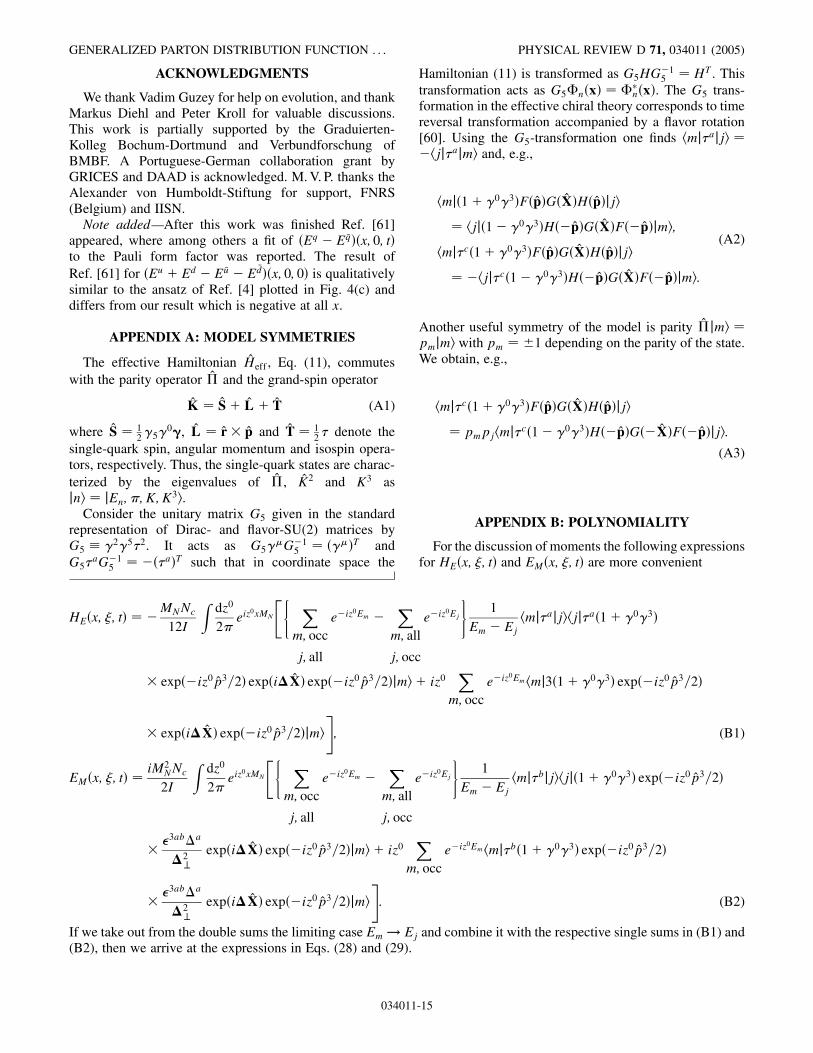
PHYSICAL REVIEW D 71, 034011 (2005)

Generalized parton distribution function �Eu �Ed��x; �; t� of the nucleonin the chiral quark soliton model

J. Ossmann,1 M. V. Polyakov,2,3 P. Schweitzer,1 D. Urbano,4,5 and K. Goeke1

1Institut fur Theoretische Physik II, Ruhr-Universitat Bochum, Germany2Universite de Liege au Sart Tilman, B-4000 Liege 1, Belgium

3Petersburg Nuclear Physics Institute, Gatchina, St. Petersburg 188350, Russia4Faculdade de Engenharia da Universidade do Porto, P-4000 Porto, Portugal

5Centro de Fısica Computacional, Universidade de Coimbra, P-3000 Coimbra, Portugal(Received 19 November 2004; published 14 February 2005)

1550-7998=20

The unpolarized spin-flip isoscalar generalized parton distribution function �Eu � Ed��x; �; t� is studiedin the large-Nc limit at a low normalization point in the framework of the chiral quark-soliton model. Thisis the first study of generalized parton distribution functions in this model, which appear only at thesubleading order in the large-Nc limit. Particular emphasis is put therefore on the demonstration of thetheoretical consistency of the approach. The forward limit of �Eu � Ed��x; �; t� of which only the firstmoment–the anomalous isoscalar magnetic moment of the nucleon–is known phenomenologically, iscomputed numerically. Observables sensitive to �Eu � Ed��x; �; t� are discussed.

DOI: 10.1103/PhysRevD.71.034011 PACS numbers: 13.60.Hb, 12.38.Lg, 12.39.Ki, 14.20.Dh

I. INTRODUCTION

The study of generalized parton distribution functions(GPDs) [1] (see [2–5] for reviews) promises numerousnew insights in the internal structure of the nucleon [6–8]. GPDs can be accessed in a variety of hard exclusiveprocesses [9] on which recently first data became available[10]. Current efforts [11] to understand and interpret thedata rely, at the early stage of art, on modeling Ansatze forGPDs–which have to comply with the severe generalconstraints imposed by the polynomiality and positivityproperties of GPDs [12,13]. Model calculations [14–21]can provide important guidelines for such Ansatze–inparticular in the case of those GPDs for which not eventhe forward limit is known from deeply inelastic scatteringexperiments. In this work we study the unpolarized GPDEa�x; �; t� in the chiral quark-soliton model (�QSM)[22,23].

The model describes the nucleon in a field theoreticframework in the limit of a large number of colors Nc asa chiral soliton of a static background pion field. Numerousnucleonic properties–among others form factors [24,25] aswell as quark and antiquark distribution functions [26–34]–have been described in this model without adjustableparameters, typically to within an accuracy of (10%-30%).The field-theoretical character is a crucial feature of the�QSM which is responsible for the wide range of applica-bility and which guarantees the theoretical consistency ofthe approach. In Refs. [15–17] it was demonstrated that the�QSM consistently describes those GPDs, which are ofleading order in the large Nc-limit.

In this work we extend the formalism of Ref. [15] to thedescription of unpolarized GPDs which appear only atsubleading order in the large-Nc expansion. We pay par-ticular attention to the demonstration of the consistency ofthe approach. After checking explicitly that the model

05=71(3)=034011(20)$23.00 034011

expressions for GPDs satisfy polynomiality, relevant sumrules, etc., we focus on the flavor combination of Ea�x; �; t�subleading in large-Nc, namely, the flavor singlet, which–being related to the spin sum rule of the nucleon–is ofparticular phenomenological interest. The correspondingflavor structure �Eu � Ed��x; �; t�, which is leading in Nc,was already studied in Ref. [15] (cf. [4]). An interestingissue we shall finally address is, which hard exclusivereactions are particularly sensitive to the GPD �Eu �Ed��x; �; t�. We observe that target single transverse spinasymmetries in two pion production are most promising inthis respect.

This paper is organized as follows. After a generaldiscussion of the properties of GPDs in Sec. II and a shortintroduction to the �QSM in Sec. III, we review in Sec. IVthe formalism of the �QSM for GPDs of leading order inNc. In Sec. V we generalize the approach to the case ofGPDs subleading in Nc, and check its consistency. InSec. VI we apply the approach to the numerical calculationof the forward limit of �Eu � Ed��x; �; t� and discuss phe-nomenological implications from our result in Sec. VII.Finally, Sec. VIII contains a summary and conclusions.Technical details on the calculations can be found in theAppendices.

II. THE UNPOLARIZED GENERALIZED PARTONDISTRIBUTION FUNCTIONS

The unpolarized quark GPDs in the proton are defined asZ d�2 ei�xhP0; s0j � q

��n2

�n6��n2;�n2

� q

��n2

�jP; si

Hq�x; �; t� �U�P0; s0�n6 U�P; s� � Eq�x; �; t� �U�P0; s0�

�i��n��

2MNU�P; s�; (1)

-1 2005 The American Physical Society

OSSMANN, POLYAKOV, SCHWEITZER, URBANO, AND GOEKE PHYSICAL REVIEW D 71, 034011 (2005)

where �z1; z2 denotes the gauge-link, and the renormaliza-tion scale dependence is not indicated for brevity. Thelightlike vector n� satisfies n�P0 � P� 2. The skewed-ness parameter �, the four-momentum transfer �� and theMandelstam variable t are defined as �� P0 � P��,n� �2�, t �2. The antiquark distributions are givenby H �q�x; �; t� �Hq��x; �; t� and similarly forE �q�x; �; t�. The unpolarized GPDs are normalized to thecorresponding elastic (Dirac- and Pauli-) form factorsZ 1

�1dxHq�x; �; t� Fq1 �t�;

Z 1

�1dxEq�x; �; t� Fq2 �t�:

(2)

The relations (2) are special cases of the polynomialityproperty [2] which follows from hermiticity, parity, timereversal and Lorentz invariance, and implies that the Nth

Mellin moment of an unpolarized GPDs is a polynomial ineven powers of � of degree less than or equal to NZ 1

�1dxxN�1Hq�x; �; 0� hq�N�0 � hq�N�2 �2 � . . .

�

�hq�N�N �N for N evenhq�N�N�1�

N�1 for N odd;

(3)

Z 1

�1dxxN�1Eq�x; �; 0� eq�N�0 � eq�N�2 �2 � . . .

�

�eq�N�N �N for N eveneq�N�N�1�

N�1 for N odd:

(4)

As a consequence of the spin 12 nature of the nucleon the

coefficients in front of the highest power in � for evenmoments N are related to each other by

hq�N�N �eq�N�N Z 1

�1dzzN�1Dq�z�; (5)

and arise from the so-called D-term Dq�z� with z x=�which has finite support only for jxj< j�j [35]. TheD-term governs the asymptotics of unpolarized GPDs inthe limit of a large renormalization scale [4] and is relatedto the distribution of the pressure and shear forces acting onthe partons in the nucleon [8].

In the large-Nc limit different flavor combinations ofGPDs and of the D-term exhibit the behavior [4]

�Hu �Hd��x; �; t� N2cf�Ncx;Nc�; t�;

�Hu �Hd��x; �; t� Ncf�Ncx;Nc�; t�;

�Eu � Ed��x; �; t� N2cf�Ncx;Nc�; t�;

�Eu � Ed��x; �; t� N3cf�Ncx;Nc�; t�;

�Du �Dd��z� N2cf�z�; �Du �Dd��z� Ncf�z�:

(6)

The functions f�u; v; t� and f�z� (which are of order O�N0c�

034011

and which we do not distinguish for notational simplicity)are stable in the large-Nc limit for fixed values ofu; v; z; t O�N0

c�. Eq�x; �; t� is systematically enhancedby one order in Nc with respect to Hq�x; �; t� due to thenucleon mass MN O�Nc� appearing in the denominatoron the right-hand side of Eq. (1). As a consequence theflavor combination of Hq�x; �; t� leading in Nc, namely�Hu �Hd��x; �; t�, and the flavor combination ofEq�x; �; t� subleading in Nc, namely �Eu � Ed��x; �; t�,have the same order in Nc. This is natural from the pointof view of the spin sum rule [6]Z 1

�1dxx

Xqu;d;...

�Hq � Eq��x; �; t� 2JQ; (7)

where 2JQ is the fraction of the nucleon spin due to (spinand orbital angular momentum of) quarks. The flavorsinglets of Eq�x; �; t� and Hq�x; �; t� enter the left-handside of (7) and contribute on equal footing in thelarge-Nc limit to JQ O�N0

c�.In the forward limit of Hq�x; �; t� we recover the unpo-

larized parton distribution function fq1 �x�

lim�! 0t ! 0

Hq�x; �; t� fq1 �x�: (8)

The GPD Eq�x; �; t� has also a well defined forward limitwhich, however, is not accessible in deeply inelastic leptonnucleon scattering. Phenomenologically only the first mo-ment of Eq�x; 0; 0� is known which is given by the anoma-lous magnetic moment &q � Fq2 �0� withZ 1

0dx�Eu � E �u��x; 0; 0� &u 1:673;

Z 1

0dx�Ed � E �d��x; 0; 0� &d �2:033:

(9)

III. THE CHIRAL QUARK-SOLITONMODEL (�QSM)

The effective chiral relativistic field theory underlyingthe �QSM is given by the partition function [36,37]

Zeff Z

D D � DU exp

"iZ

d4x � �i@6 �MU)5�

#;

(10)

where and U exp�i*a a� are the SU(2) chiral quarkand pion fields with U)5 � exp�i)5*

a a�, and M is thedynamical quark mass. The effective theory (10) wasderived from the instanton model of the QCD vacuum[37,38]. An important small parameter in this derivationis the instanton packing fraction +av=Rav �

13 of the dilute

instanton medium, where +av and Rav are, respectively, theaverage size and separation of instantons. The effectivetheory (10) contains the Weinberg-Gasser-Leutwyler

-2

GENERALIZED PARTON DISTRIBUTION FUNCTION . . . PHYSICAL REVIEW D 71, 034011 (2005)

Lagrangian and the Wess-Zumino term with correct coef-ficients and is valid for momenta below a scale set by theinverse of the average instanton size +�1

av � 600 MeV. Atthis scale the dynamical quark massM, which in general ismomentum dependent, drops to zero. In numerical calcu-lations it is often convenient to consider constant M and toapply an appropriate regularization method with an UV-cutoff of the order of magnitude of +�1

av . In calculations of(some) GPDs, however, it is important to consider momen-tum dependent M [15].

In the large-Nc limit, which allows one to solve thefunctional integral over pion field configurations in thesaddle-point approximation, the effective theory inEq. (10) describes the nucleon as a classical soliton ofthe pion field [22] providing a practical realization of thelarge-Nc picture of the nucleon [39]. Quarks are describedby one-particle wave functions which are the solutions ofthe Dirac equation in the background of the static pion field

H eff jni Enjni; Heff �i)0)k@k � )0MU)5 :

(11)

The spectrum of the effective Hamiltonian (11) consists ofan upper and a lower Dirac continuum, which are distortedby the background field compared to the continua of thefree Hamiltonian H0 �i)0)k@k � )0M, and of a dis-crete bound state level of energy Elev. By occupying thediscrete level and the states of lower continuum each byNcquarks in an antisymmetric color state, one obtains a statewith unity baryon number called soliton. The minimizationof the soliton energy Esol with respect to variations of thechiral fieldU yields the self-consistent pion fieldUc, whichfor symmetry reasons has the ‘‘hedgehog’’ structureUc�x� exp�ier*P�r� where P�r� is the soliton profilewith r jxj and er x=r. The mass of the nucleon isgiven by

MN Esol�Uc minUEsol�U ;

Esol�U Nc

"Elev �

XEn < 0

�En � En0�

#reg

:

(12)

The soliton energy is (for constant M) logarithmically UV-divergent and has to be regularized–as indicated inEq. (12) and described in Ref. [25].

In order to include 1=Nc corrections one has to considerquantum fluctuations around the saddle-point solution.Hereby the (translational and rotational) zero modes ofthe soliton solution are the only taken into account. Inparticular one considers time-dependent rotations of thehedgehog field, Uc�x� ! R�t�Uc�x�Ry�t�, where the col-lective coordinate R�t� is a rotation matrix in SU(2)-flavorspace. The path integration over the collective coordinatescan be solved by expanding in powers of the collectiveangular velocity " � �iRy@tR which corresponds to an1=Nc expansion. The latter is justified, since the soliton

034011

moment of inertia,

I Nc6

Xn; occj; non

hnj*ajjihjj*ajniEj � En

; (13)

is large, namely I O�Nc�, and the soliton rotation istherefore slow. [In Eq. (13) one has to sum over occupied(’’occ’’) states n, i.e., over states with En � Elev, and overnonoccupied (’’non’’) states j, i.e., over states with Ej >Elev.] This procedure–which is referred to as quantizationof zero modes–assigns to the soliton a definite momentumand spin-isospin quantum numbers [22].

The effective theory (10) allows one to derive by meansof path integral methods unambiguous model expressionsfor nucleon matrix elements of QCD quark bilinear opera-tors sandwiched in nucleon states hN0j � �z1��z1; z2 $ �z2�jNi, where $ is some matrix in Dirac- andflavor space. For local observables such as, e.g., formfactors the gauge-link reduces to a unity matrix in colorspace. When evaluating nonlocal operators in the model–as they appear in GPDs–it is crucial that the effects ofgluonic degrees of freedom, which are intrinsic in thegauge-link, appear strongly suppressed with respect toquark degrees of freedom. This is true for twist-2 [40](and certain twist-3 operators [41]) and guarantees thecolor gauge invariance of the model calculation.

If in QCD hN0j � �z1��z1; z2 $ �z2�jNi is scale dependentthen the model result corresponds to low a scale of +�1 �600 MeV. In this way static nucleonic observables [24,25],twist-2 quark and antiquark distribution functions [26–34]have been computed in the �QSM and found to agree towithin (10%-30%) with experimental data or phenomeno-logical parametrizations. In [15,16] the approach was gen-eralized to describe GPDs. The results of the �QSMrespect all general counting rules of the large-Ncphenomenology.

IV. GPDS IN LEADING ORDER OF LARGE Nc

It is convenient to treat the cases of flavor singlet andnonsinglet quantities in the model separately for symmetryreasons. Let us introduce the notation

M �I0�s0s �

Z d�2

ei�xhP0; s0j � ��n2

�n6

��n2

�jP; si (14)

M �I1�s0s �

Z d�2

ei�xhP0; s0j � ��n2

�*3n6

��n2

�jP; si:

(15)

The M�I�s0s are 2 � 2-matrices in spin indices which have

the following behavior in the large-Nc limit

trfM�I0�g O�N2c�; trf�mM�I0�g O�Nc�;

trfM�I1�g O�Nc�; trf�mM�I1�g O�N2c�:

(16)

-3


These relations do not follow from the dynamics of themodel, but are group theoretical consequences of the spin-flavor structure of the (hedgehog) soliton field. In this sensethe relations (16) are model-independent large-Nc resultsof QCD [42] which are consequently respected in the�QSM.

In order to evaluate the bi(nucleon-)spinor expression onthe right-hand side of Eq. (1) one has to consider that in thelarge Nc limit the nucleon is heavy, MN O�Nc�, and thekinematics becomes nonrelativistic. In particular we havefor the components of the momentum transfer �i O�N0

c�and �0 O�N�1

c �. Thus the hierarchy holds MN �j�ij � j�0j, while t ��2 O�N0

c� and � ��3=�2MN� O�N�1

c �. Here we have chosen n� �1; 0; 0;�1�=MN . Evaluating consequently the right-handside of Eq. (1) in this large-Nc kinematics yields for theflavor-singlet and nonsinglet case, respectively,

M�I0�s0s 23ss0 �Hu �Hd��x; �; t� �

i43kl�k

MN��l�s0s

� ��Hu �Hd��x; �; t� � �Eu � Ed��x; �; t� ;

(17)

M�I1�s0s 23ss0

��Hu �Hd��x; �; t� �

t

4M2N

�Eu � Ed�

� �x; �; t��i43kl�k

MN��l�s0s�Eu � Ed��x; �; t�:

(18)

From Eqs. (17) and (18), simple relations follow for theleading (in the large-Nc counting) GPDs

�Hu �Hd��x; �; t� 1

4trfM�I0�g; (19)

�Eu � Ed��x; �; t� iMN4

3bm�b

2�2?

trf�mM�I1�g; (20)

where ‘‘tr’’ denotes the trace over spin indices and �2?

�2 � ��3�2 �t� 4M2N�

2. The subleading structures,however, appear only in combination with the leading ones

�Hu �Hd��x; �; t� � �Eu � Ed��x; �; t�

iMN4

3bm�b

2�2?

trf�mM�I0�g; (21)

�Hu �Hd��x; �; t� �t

4M2N

�Eu � Ed��x; �; t�

1

4trfM�I1�g: (22)

The structures in the square brackets of Eqs. (17) and (18),and on the left-hand-sides of Eqs. (21) and (22), are ana-logs of the relations between the electric and magnetic

034011

form factors GqE�t�; G

qM�t� and the Dirac- and Pauli-form

factors Fq1 �t�; Fq2 �t�, which are given by

GqE�t� Fq1 �t� � Fq2 �t�; G

qM�t� Fq1 �t� �

t

4M2N

Fq2 �t�:

(23)

The model expressions for M�I0;1� in leading order ofthe large-Nc limit were derived in Ref. [15] and the follow-ing results for �Hu �Hd��x; �; t� and �Eu � Ed� were ob-tained using Eqs. (17) and (18),

�Hu �Hd��x; �; t� MNNcZ dz0

2

Xn; occ

eiz0�xMN�En�hnj

� �1 � )0)3� exp��i

z0

2p3

�

� exp�i�X� exp��i

z0

2p3

�jni; (24)

�Eu � Ed��x; �; t� 2iM2

NNc3��?�2

�Z dz0

2

Xn; occ

eiz0�xMN�En�hnj

� �1 � )0)3��3

� exp��i

z0

2p3

�exp�i�X�

� exp��i

z0

2p3

�jni: (25)

There are equivalent expressions withP

occ ! �P

non, i.e.,where the summation goes over nonoccupied states En >Elev. The possibility of computing in the model quantitiesin these two independent ways is deeply related to thelocality properties of the model [26]. Numerical resultsfor (24) and (25), were presented in Ref. [15], and furtherdiscussed and reviewed in Ref. [4].

Let us emphasize that according to Eq. (8) in the forwardlimit the right-hand side of (24) reduces to the modelexpression for �fu1 � fd1 ��x� [15]. �Hu �Hd��x; �; t� and�Eu � Ed��x; �; t� are correctly normalized to the respec-tive form factors [15] cf. Eq. (2), and they satisfy thepolynomiality conditions in Eqs. (3) and (4) [17].

It is worthwhile mentioning that the coefficient of thehighest power in � of even Mellin moments of �Eu �Ed��x; �; t� in leading order of large Nc is zero in the�QSM. Also this result is not a dynamical feature of themodel, but rather a group theoretical consequence of thesoliton symmetries which ensure the correct large-Nccounting for the flavor-nonsinglet D-term. In fact, if thiscoefficient were not zero, then �Eu � Ed� O�N3

c� would

-4


imply �Du �Dd� O�N3c� in conflict with the counting

rule which states �Du �Dd� O�Nc� cf. Eq. (6).

V. GPDS IN SUBLEADING ORDER OF LARGE Nc

One has to consider 1=Nc (rotational) corrections toM�I0;1� in order to study the subleading flavor combina-tions �Hu �Hd��x; �; t� and �Eu � Ed��x; �; t�. In order tosimplify the notation let us introduce

EM�x; �; t� �Hu �Hd��x; �; t� � �Eu � Ed��x; �; t�

�O�N2c�; (26)

034011

HE�x; �; t� �Hu �Hd��x; �; t� � �Eu � Ed��x; �; t�t

4M2N

�O�Nc�: (27)

Here the respective already known (see above) flavor com-binations ofHq�x; �; t� and Eq�x; �; t� leading inNc appear.Thus it is sufficient to focus on the ‘‘new’’ objectsEM�x; �; t� and HE�x; �; t�.

The model expressions for HE�x; �; t� and EM�x; �; t�(for a proton) read

HE�x; �; t� �MNNc12I

Z dz0

2

"( Xm; occj; allm � j

e�iz0Em �

Xm; allj; occm � j

e�iz0Ej

)1

Em � Ej�

@@xMN

Xm; occj; allm � j

e�iz0Em

#eiz

0xMN hmj*ajji

� hjj*a�1 � )0)3� exp��iz0p3=2� exp�i�X� exp��iz0p3=2�jmi;

(28)

EM�x; �; t� iM2

NNc2I

Z dz0

2

"( Xm; occ

j; all

m � j

e�iz0Em �

Xm; all

j; occ

m � j

e�iz0Ej

)1

Em � Ej�

@@xMN

Xm; occ

j; all

m � j

e�iz0Em

#eiz

0xMN hmj*bjjihjj

� �1 � )0)3� exp��iz0p3=2�43ab�a

�2?

exp�i�X� exp��iz0p3=2�jmi: (29)

There are equivalent expressions with opposite sign wherethe summations go over nonoccupied states. Consideringthe generalizations due to the off-forward kinematics[15,16], the derivations of Eqs. (28) and (29) closely followthe derivations of the model expression for the flavor non-singlet unpolarized distribution �fu1 � fd1��x� [30] and theflavor-singlet helicity �gu1 � gd1��x� and transversity �hu1 �hd1��x� distribution functions [33]. In the following wecheck explicitly the theoretical consistency of the expres-sions (28) and (29).

A. Form factors and polynomiality

Let us first verify the correct normalization ofHE�x; �; t�andEM�x; �; t�. In order to integrate Eqs. (28) and (29) overx it is convenient to substitute x! y xMN and to extendthe y-integration range ��MN;MN to ��1;1 in thelarge-Nc limit. The derivative in x drops out and aftercancellations in the curly brackets in Eqs. (28) and (29),only summations over occupied states jmi and nonoccu-pied states jji and vice versa remain, which can be com-bined by exploring model symmetries, see Appendix A.We obtain

Z 1

�1dxHE�x; �; t� �

Nc6I

Xm; occj; non

1

Em � Ejhmj*ajjihjj*a exp�i�X�jmi � G�I1�

E �t�;

Z 1

�1dxEM�x; �; t�

NcMN

2I�2

Xm; occj; non

i4abc�a

Em � Ejhmj*bjjihjj)0)c exp�i�X�jmi � 3G�I0�

M �t�;

(30)

where we identify the model expressions for the electricisovector G�I1�

E �t� and magnetic isoscalar G�I0�M �t� form

factors [24,25]. [The factor 3 in the second line of (30)appears because for GPDs the notion of (non-) singlet

commonly refers to quark flavors, e.g., �Hu �Hd�. Incontrast, in the case of form factors it refers to protonand neutron, e.g., G�I0�

M � GpM �Gn

M.] From (23), (26),(27), and (30), and recalling that the leading large-Nc

-5


GPDs �Hu �Hd��x; �; t� and �Eu � Ed��x; �; t� are cor-rectly normalized [15], we find for the subleading GPDsin agreement with Eq. (2)

Z 1

�1dx�Hu �Hd��x; �; t� �Fu1 � Fd1 ��t�;Z 1

�1dx�Eu � Ed��x; �; t� �Fu2 � Fd2 ��t�:

(31)

In Appendix B it is explicitly demonstrated that the highermoments in x of HE�x; �; t� and EM�x; �; t� are even poly-nomials in � according to (3) and (4). In fact, we find that ineven moments the coefficients in front of the highest powerin � have opposite sign in �Eu � Ed��x; �; t� and �Hu �Hd��x; �; t� in accordance with the relation (5).

B. Spin sum rule

For the second moment of EM�x; �; t� at t 0 we obtainin the �QSM cf. Appendix C

Z 1

�1dxxEM�x; �; 0� 2SQ � 2LQ 2SN 1; (32)

where SN 12 is the total spin of the nucleon, and SQ and

LQ are the respective contributions of the spin and orbitalangular momentum of quarks and antiquarks to the nu-cleon spin. The result in Eq. (32) is consistent. In theeffective theory the contribution of quark and antiquarkdegrees of freedom, JQ SQ � LQ, must account entirelyfor the nucleon spin, since there are no gluons in the model.Thus, the result in (32) means that the spin sum rule (7) isconsistently fulfilled in the model:

Z 1

�1dxx�Hu �Hd � Eu � Ed��x; �; 0� 2JQ 1: (33)

We note that in the model 2SQ g�0�A 0:35, where g�0�Adenotes the isosinglet axial coupling constant [33]. Thus,in the �QSM 35% of the nucleon spin are due to the quarkspin, while 65% are due to the orbital angular momentumof quarks and antiquarks.

In a gauge theory it is not possible to separate unambig-uously spin and orbital momentum [43,44]. It also is by nomeans clear that the identification of the model expressionfor quark orbital momentum in Eq. (32) is unambiguous. Itis interesting to note that one arrives at the same result byintuitively identifying Li 4ijkxjpk with the orbital angu-lar momentum operator of the effective theory (10) cf. [45].However, one has to keep in mind that this issue canrigorously be studied in the instanton vacuum modelfrom which the �QSM was derived. Noteworthy in thiscontext is that g�0�A in the chiral quark-soliton model arisesfrom the realization of the axial anomaly in the instantonvacuum [40].

034011

Since in the chiral quark-soliton model also the totalmomentum of the nucleon is carried by quarks and anti-quarks only [26], i.e., MQ 1, we obtain for the secondmoment of �Eu � Ed��x; 0; 0� the resultZ 1

�1dxx�Eu � Ed��x; 0; 0� �2JQ �MQ� 0: (34)

Interestingly, the result (34) holds also in QCD in theasymptotic limit of a large normalization scale �! 1.This happens because MQ and 2JQ have the same asymp-totics [43]

lim�!1

MQ lim�!1

�2JQ� 3NF

16 � 3NF(35)

where NF is the number of quark flavors. It should bestressed, however, that at a low scale �� 600 MeV inthe model MQ 2JQ 1 is far from the asymptotic val-ues in Eq. (35).

Equation (34) is the general prediction of any modellacking explicit gluon degrees of freedom, which is able toconsistently describe the nucleon in terms of quark andantiquark degrees of freedom–such as the �QSM. One canshow, using methods of theory of the instanton vacuum[40] that the gluon contribution to the nucleon momentumand angular momentum is parametrically suppressed bythe packing fraction of the instantons in the vacuum.Therefore in order to obtain nonzero gluon contributionsone has to extend �QSM beyond the leading order in theinstanton packing fraction.

Noteworthy, it has been argued that momentum andangular momentum should be equally distributed amongquarks and gluons at any scale, not only in the asymptoticlimit (35), an observation which can be reformulated as theabsence of an anomalous gravitomagnetic moment of thenucleon [46].

C. Forward limit

Finally let us discuss the forward limit. From (27) we seethat HE�x; 0; 0� �Hu �Hd��x; 0; 0�. Indeed, taking � !0 in Eq. (28) and making use of the hedgehog symmetry werecover, in agreement with Eq. (8), the model expressionfor the flavor nonsinglet unpolarized distribution function[30]

HE�x; 0; 0� MNNc12I

Xm; occ

j; all

m � j

�2

Ej � Em�

@@xMN

�hmj*ajji

� hjj*a�1 � )0)3�3�xMN � Em � p3�jmi

� �fu1 � fd1 ��x�: (36)

The forward limit of EM�x; �; t� ! �Eu � Ed��x; 0; 0� ��fu1 � fd1 ��x� contains a contribution which is a priori notknown, namely �Eu � Ed��x; 0; 0�. Therefore we derive

-6

Cocc

Elev

C

ωRe

Imω

pos. cont.

neg. cont.


here the model expression for EM�x; 0; 0� which we shallstudy below in detail. The limit �! 0 is regular,1 however,to complete the forward limit we have to consider with carethe limit �? ! 0 of the structure

43jk�j?

�2?

exp�i�?X?� 43jk �j?

�2?

� i43jkXm?�j

?�m?

�2?

�O��k�: (37)

The first term in the above expansion (for small but non-zero �?) yields a vanishing result when inserted intoEq. (29) due to the hedgehog symmetry. The second termfrom the expansion in (37) yields the only contributionwhich survives the forward limit in Eq. (29). Making use of

lim�?!0

�j?�m

?

�2?

1

23jm? �

1

2�3jm � 3j33m3� (38)

we obtain upon use of hedgehog symmetry

EM�x; 0; 0� M2NNc4I

43jkX

m; occ

j; all

m � j

�2

Ej � Em�

@@xMN

�

� hmj*kjjihjj�1 � )0)3�

� 3�xMN � Em � p3�Xj?jmi: (39)

As a final check we integrate EM�x; 0; 0� in Eq. (39) over xand recover the model expression for the isoscalar mag-netic moment [48]Z 1

�1dxEM�x; 0; 0�

MNNc2I

Xm; occ

j; non

1

Ej � Emhmj*3jji

� hjj)0�� X�3jmi

3��T0�: (40)

VI. THE FORWARD LIMIT OF �Eu �Ed��x; �; t�

In order to compute the forward limit �Eu � Ed��x; 0; 0� � EM�x; 0; 0� � �fu1 � fd1 ��x� we have to numeri-cally evaluate the model expression (39) for EM�x; 0; 0�.The distribution function �fu1 � fd1 ��x� was already studiedin [26,28,29]. The numerical methods needed for that weredeveloped in Refs. [28–30] in the context of usual partondistributions functions in leading and subleading order ofthe large-Nc expansion. We restrict ourselves to the for-ward limit since this numerical technic does not allow afull calculation of GPDs for all values of � and t.

1Of course, by limiting oneself to � 0 one drops importantphysics. E.g., the skewedness parameter is related to the corre-lation length between partons, see [47] and references therein.The present calculation unfortunately cannot shed any light inthis respect.

034011

A. Gradient expansion and chiralenhancement of GPDs

Before studying the model expression (29) numericallyin the model we shall consider the gradient expansion ofEM�x; �; t�. This expansion consists in expanding modelexpressions in powers of the gradients of the (static) chiralfield rU. Such an expansion would quickly converge if thesoliton field were slowly varying, i.e., if the soliton werelarge rU� 1=Rsol � M where Rsol is the scale character-izing the soliton size. However, for the physical solitonsolution Rsol � 1=M. Nevertheless the gradient expansionis instructive and allows–among others–to study the UV-behavior of the model expressions. Also, as we shall seebelow, the gradient expansion allows one to obtain strongenhancement of GPD EM�x; �; t� in the region of small x.This enhancement is related to the effect of the pion cloud.

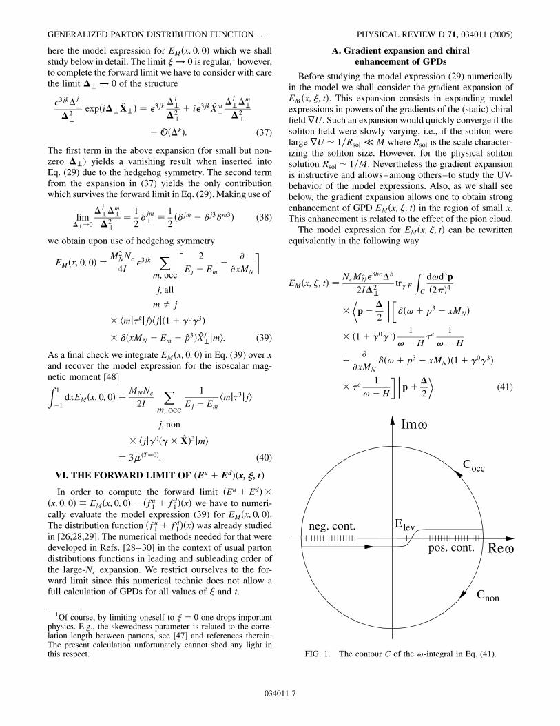
The model expression for EM�x; �; t� can be rewrittenequivalently in the following way

EM�x; �; t� NcM

2N4

3bc�b

2I�2?

tr);FZC

d!d3p�2 �4

�

p�

�2

��3�!� p3 � xMN�

� �1 � )0)3�1

!�H*c

1

!�H

�@

@xMN3�!� p3 � xMN��1 � )0)3�

� *c1

!�H

��p��2

�(41)

non

FIG. 1. The contour C of the !-integral in Eq. (41).

-7


where ‘‘tr);F’’ denotes the trace over Dirac- and flavorindices. The contour C is defined in Fig. 1. Closing thecontour C in the upper half of the complex !-plane yieldsthe expression in Eq. (29), closing it in the lower half planeone obtains the equivalent expression where the summa-

2For that we rewrite the operator 1=�!�H� 12 �

�!�H�=�!2 �H2�� 12 �!

2 �H2��1�!�H� where H2 p2 �M2 � iM�rU)5 , and expand it in powers of iM�rU)5 .Such a ‘‘symmetric expansion’’ of 1=�!�H� ensures the her-miticity of the operator also in the case when the series in rU istruncated.

034011

tion goes over nonoccupied states m cf. the sequence ofEq. (29).

Expanding the expression in Eq. (41) in powers of rUone obtains2 already from the zeroth order in �rU� thefollowing result for the continuum contribution

EcontM �x; �; t�

M2Nf

2

4I�?2

Z d3k�2 �3

f�k�

�2

�f�k�

�2

��2k3 � �3��k�

�

�%�xMN � k3�%�� x� � %��xMN � k3�%�x� ��

k3 � �MN

� ��$ �� %�x� ��%��x� �� %��x� ��%�x� ��

2�MN

��O�rU� (42)

3

where f�q� f�jqj� is one of the functions describing theFourier transform of the U�x�-fieldZ

d3x�U�x� � 1 e�iqx g�q� �i�qjqj

f�q�;

f�q� � 4 Z 1

0drr2j1�rjqj� sinP�r�:

(43)

Note that the property EM�x; �; t� EM�x;��; t� holdsmanifestly for the result in Eq. (42).

In the derivation of Eq. (42) we encountered a logarith-mic UV-divergence proportional to M2. This UV-divergence can be regularized, e.g., by means of a Pauli-Villars subtraction as

EcontM �x; �; t�reg Econt

M �x; �; t;M�

�M2

M2PV

EcontM �x; �; t;MPV�: (44)

We removed the dependence of the result on cutoff andregularization scheme in favor of a physical parameter,namely, the pion decay constant f 93 MeV given inthe effective theory (10) by the (Euclidean loop) integral

f2

Z d4pE�2 �4

4NcM2

�p2E �M2�2

jreg (45)

which exhibits a similar UV-behavior and can be regular-ized analogously. In the first order of the gradient expan-sion, indicated only symbolically as O�rU� in Eq. (42), wealso encounter a logarithmic divergence which can beremoved by means of (44). Still higher orders in thegradient expansion yield finite results–as one can concludefrom dimensional counting. (Or from the fact that the

isoscalar magnetic moment appears at the order �rU�2

and is UV-finite cf. Ref. [23].)Equation (42) may give at best only a rough estimate for

EM�x; �; t�. Nevertheless it contains already main featuresof the total result. Apart from the UV-properties, which wediscussed above, the small x- behavior in the chiral limit isof interest since the exact numerical calculation is per-formed under such conditions. The soliton profile behavesat large distances as

P�r� �B

r2�1 �m r� exp��m r�;

B 3g�3�A8 f2

for r�

��B

p (46)

with B related to axial isovector coupling constant g�3�A 1:26 by means of equations of motion. The large distancebehavior (46) of the soliton profile translates into theinfrared- behavior of the function f�q� as

f�q� �3g�3�A2f2

1

q2 �m2

for small q2; m2 � B�1:

(47)

Note that B�1 < �4 f �2 � 1 GeV2 which is a typicalscale for chiral symmetry breaking effects. Apparentlythe limits m ! 0 and q ! 0 do not commute.3 In theforward limit in Eq. (42) this means

The noncommutativity of such limits is known, e.g., fromstudies of the polarized photon structure function, where thevirtuality of the photon plays the role of the momentum q. In thatcase it is known that the correct order of limits is to take first thephoton virtuality to zero, and only then to consider m ! 0 [49].However, in our context it is not clear in which order the limitsshould be taken, though phenomenology may suggest first totake q ! 0 while m is kept finite.

-8


EM�x; 0; 0� M2Nf

2

6I�2 �2Z 1

jxMN jdqq2f�q�2

�1 �

jxMNj

q

�

� x!0

�3g�3�A8 f

�2MN

I�

(1x for m 0 2MNm

for m � 0:

(48)

Note that the soliton moment of inertia could be eliminatedin favor of the �-nucleon mass-splitting as M� �MN 3=�2I�.

Although derived in the leading order of the gradientexpansion of model expressions Eq. (48) is of more general

034011

nature as it is related to the effect of pion cloud. Thereforeit should be possible to derive the above expression bymeans of chiral perturbation theory. Another interestingquestion is to find phenomenological manifestations of thechiral enhancement. This would open new exciting possi-bilities to investigate chiral symmetry breaking in the hardexclusive processes.

B. Numerical calculation

As any quantity in the model, EM�x; 0; 0� is composed ofa contribution of the discrete level and of the continuumcontribution defined, respectively, as

ElevM �x; 0; 0�

M2NNc4I

43jkXEj; all

j � lev

�2

Ej � Elev�

@@xMN

�hlevj*kjjihjj�1 � )0)3�3�xMN � Em � p3�Xj?jlevi

EcontM �x; 0; 0�

M2NNc4I

43jkX

Em < 0

Ej; all

m � j

�2

Ej � Em�

@@xMN

�hmj*kjjihjj�1 � )0)3�3�xMN � Em � p3�Xj?jmi

�M2NNc4I

43jkX

Em > 0

Ej; all

m � j

�2

Ej � Em�

@@xMN

�hmj*kjjihjj�1 � )0)3�3�xMN � Em � p3�Xj?jmi

(49)

For a constant (momentum-independent) M the continuumcontribution to EM�x; �; t� is UV-divergent. It can be regu-larized by means of a single Pauli-Villars subtraction ac-cording to Eq. (44).In the context of parton distributionfunctions the Pauli-Villars method is the preferred regu-larization scheme because it preserves fundamental prop-erties of parton distributions such as sum rules, positivity,etc. [26]. It should be noted that the contribution of thediscrete level, which is always finite, must not be regular-ized [29].

The numerical method to evaluate EM�x; 0; 0� consists ofplacing the soliton in a large but finite spherical box,introducing free basis states (eigenstates of the freeHamiltonian, see Eq. (11) and below), and discretizingthe basis by imposing appropriate boundary conditions

following Kahana and Ripka [50]. The full Hamiltonian(11) can be diagonalized numerically in this basis [48].With the eigenfunctions and eigenstates, ,n�x� and En,one is then in a position to evaluate Eq. (49). This is mostconveniently done by converting the model expression (49)into a spherically symmetric form [28]. For that we intro-duce in (49) a unit vector a such that the original expres-sion is recovered for a e�3�,

43jk�1 � )0)3�3�xMN � Em � p3�Xj?

! �1 � )0a � )�3�xMN � Em � a � p��a� X�k: (51)

Then we average over all possible orientations of the vectora. This yields

-9


EM�x; 0; 0� �M2NNc4I

Xm; occ

j; all

m � j

�2

Em � Ej�

@@xMN

�hmj*kjjihjj

��p� X�k

I1�jpj; Em; x�jpj2

� �)0�� X�k�I0 � I2��jpj; Em; x�

2jpj� �p� X�k�)0� � p�

�3I2 � I0��jpj; Em; x�2jpj3

�jmi;

where Il�jpj� �xMN � Em�l

2jpjl%�jpj � jxMN � Emj�:

(52)

Although noncommuting operators appear in (52) never-theless the final result is a hermitian operator. The averag-ing procedure must, of course, preserve hermiticity. It isthis step which prevents us from tackling also the problemto compute numerically EM�x; �; t� for nonzero � and t. Forfinite � the appearance of an additional direction, namely,along �? perpendicular to the 3-direction, makes theresulting expressions unsuitable for a numericalevaluation.

Since we work with a discrete basis, the %-functions in(52) would lead to discontinuous functions. Therefore weconvolute the true (but due to finite size effects discontinu-ous) function with a narrow Gaussian

EsmM �x; 0; 0� 1��

p)

Z 1

�1dx0e��x�x0�2=)2

EM�x0; 0; 0�:

(53)The width ) has to be chosen adequately according to the

-10

-5

0

5

10

-1 -0.5 0 0.5 1

EM(x,0,0)

x

levelcont. occ.cont. non.

(a)

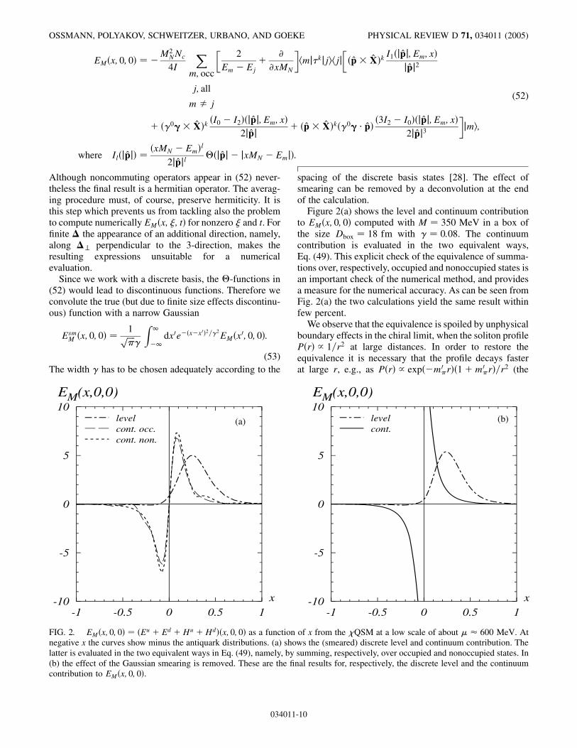
FIG. 2. EM�x; 0; 0� �Eu � Ed �Hu �Hd��x; 0; 0� as a functionnegative x the curves show minus the antiquark distributions. (a) sholatter is evaluated in the two equivalent ways in Eq. (49), namely, by(b) the effect of the Gaussian smearing is removed. These are the ficontribution to EM�x; 0; 0�.

034011

spacing of the discrete basis states [28]. The effect ofsmearing can be removed by a deconvolution at the endof the calculation.

Figure 2(a) shows the level and continuum contributionto EM�x; 0; 0� computed with M 350 MeV in a box ofthe size Dbox 18 fm with ) 0:08. The continuumcontribution is evaluated in the two equivalent ways,Eq. (49). This explicit check of the equivalence of summa-tions over, respectively, occupied and nonoccupied states isan important check of the numerical method, and providesa measure for the numerical accuracy. As can be seen fromFig. 2(a) the two calculations yield the same result withinfew percent.

We observe that the equivalence is spoiled by unphysicalboundary effects in the chiral limit, when the soliton profileP�r� / 1=r2 at large distances. In order to restore theequivalence it is necessary that the profile decays fasterat large r, e.g., as P�r� / exp��m0

r��1 �m0 r�=r

2 (the

-10

-5

0

5

10

-1 -0.5 0 0.5 1

EM(x,0,0)

x

levelcont.

(b)

of x from the �QSM at a low scale of about � � 600 MeV. Atws the (smeared) discrete level and continuum contribution. Thesumming, respectively, over occupied and nonoccupied states. Innal results for, respectively, the discrete level and the continuum

-10

4We work here with the value M 350 MeV which followsfrom instanton phenomenology [37,38] and was used in calcu-lations of parton distributions and GPDs [15–17,26–33].However, in numerous model calculations M was allowed tovary in the range �350 � 450� MeV [25]. The value M 420 MeV was somehow preferred because it reproduced exactlythe delta-nucleon mass-splitting within the proper-time regulari-zation [25].


numerical parameter m0 is not to be confused with the

physical pion mass discussed above). Since the issue ofcomputing self-consistent profiles with finite pion massesin the Pauli-Villars regularization is not yet solved cf. [51]for a discussion, we use the chiral self-consistent profilecomputed in [29] up to some rA and continue it for r > rAwith an artificial Yukawa-tail-like suppression of the abovekind. We find the results practically independent of rA andm0 in the range rA �4 � 8� fm and m0

�100 �200� MeV. This proves that what matters in this contextis only a sufficiently small value of the profile at theboundary r Dbox, and makes the extrapolations rA !1 and/orm0

! 0 superfluous, which in principle would benecessary to remove any dependence of these numericalparameters. The equivalence demonstrated in Fig. 2(a) isachieved in this way. This procedure was applied success-fully to cure an analogue problem in the calculation of thetransversity distribution [34].

Let us comment on the effect of smearing, which isnegligible whenever one deals with a continuous functionsuch as the contribution of the discrete level cf. Figs. 2(a)and 2(b). However, in the case of the continuum contribu-tion the smearing ‘‘hides’’ an 1=x singularity which be-comes apparent only in the final result after the smearing isremoved. This is done by Fourier transforming EsmM �x; 0; 0�of Eq. (53), dividing out the smearing Gaussian, and re-Fourier transforming–which yields the final results shownin Fig. 2(b).

We remark that in the �QSM the parton distributionfunctions (and forward limits of GPDs) do not vanish forjxj � 1. Instead they decay as exp��constNcx� at jxj � 1[26] which is, in fact, numerically very small even forNc 3.

C. Discussion of the results

We observe in EM�x; 0; 0� that the discrete level contrib-utes predominantly to the distribution of quarks rather thanantiquarks. The continuum, however, contributes nearlyequal portions to quark and antiquark distributions. As aresult the isoscalar magnetic moment receives a negligiblecontribution from the continuum. This strong dominanceof the level contribution in the isoscalar magnetic momentwas observed in earlier calculations [24]. The result (inunits of the nuclear magneton)

��T0� � ��p ��n� 1

3

Z 1

�1dxEM�x; 0; 0�

0:65 vs. 0:88exp; (54)

agrees with the experimental value to within 25%, i.e., towithin an accuracy typical for �QSM results [25].

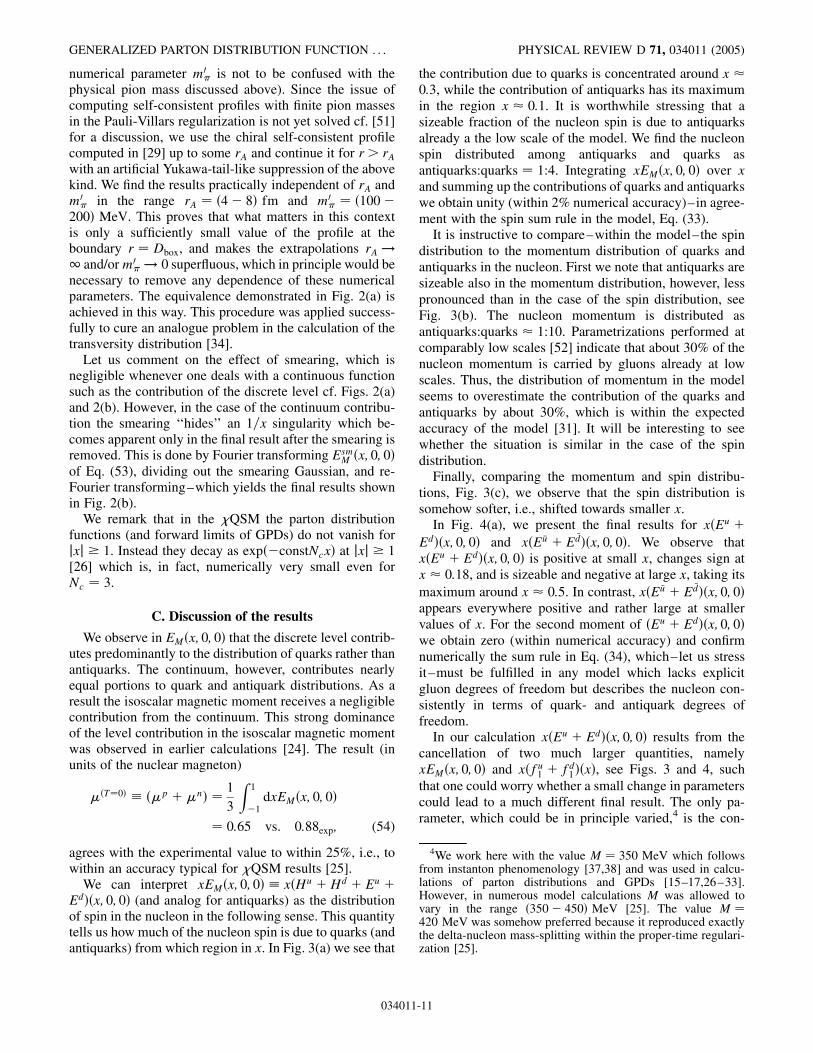
We can interpret xEM�x; 0; 0� � x�Hu �Hd � Eu �Ed��x; 0; 0� (and analog for antiquarks) as the distributionof spin in the nucleon in the following sense. This quantitytells us how much of the nucleon spin is due to quarks (andantiquarks) from which region in x. In Fig. 3(a) we see that

034011

the contribution due to quarks is concentrated around x �0:3, while the contribution of antiquarks has its maximumin the region x � 0:1. It is worthwhile stressing that asizeable fraction of the nucleon spin is due to antiquarksalready a the low scale of the model. We find the nucleonspin distributed among antiquarks and quarks asantiquarks:quarks 1:4. Integrating xEM�x; 0; 0� over xand summing up the contributions of quarks and antiquarkswe obtain unity (within 2% numerical accuracy)– in agree-ment with the spin sum rule in the model, Eq. (33).

It is instructive to compare–within the model– the spindistribution to the momentum distribution of quarks andantiquarks in the nucleon. First we note that antiquarks aresizeable also in the momentum distribution, however, lesspronounced than in the case of the spin distribution, seeFig. 3(b). The nucleon momentum is distributed asantiquarks:quarks � 1:10. Parametrizations performed atcomparably low scales [52] indicate that about 30% of thenucleon momentum is carried by gluons already at lowscales. Thus, the distribution of momentum in the modelseems to overestimate the contribution of the quarks andantiquarks by about 30%, which is within the expectedaccuracy of the model [31]. It will be interesting to seewhether the situation is similar in the case of the spindistribution.

Finally, comparing the momentum and spin distribu-tions, Fig. 3(c), we observe that the spin distribution issomehow softer, i.e., shifted towards smaller x.

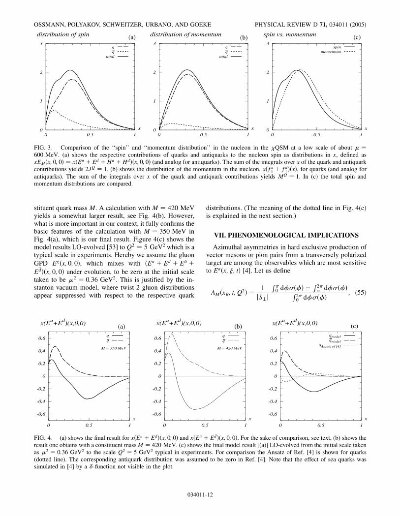
In Fig. 4(a), we present the final results for x�Eu �Ed��x; 0; 0� and x�E �u � E �d��x; 0; 0�. We observe thatx�Eu � Ed��x; 0; 0� is positive at small x, changes sign atx � 0:18, and is sizeable and negative at large x, taking itsmaximum around x � 0:5. In contrast, x�E �u � E �d��x; 0; 0�appears everywhere positive and rather large at smallervalues of x. For the second moment of �Eu � Ed��x; 0; 0�we obtain zero (within numerical accuracy) and confirmnumerically the sum rule in Eq. (34), which– let us stressit–must be fulfilled in any model which lacks explicitgluon degrees of freedom but describes the nucleon con-sistently in terms of quark- and antiquark degrees offreedom.

In our calculation x�Eu � Ed��x; 0; 0� results from thecancellation of two much larger quantities, namelyxEM�x; 0; 0� and x�fu1 � fd1 ��x�, see Figs. 3 and 4, suchthat one could worry whether a small change in parameterscould lead to a much different final result. The only pa-rameter, which could be in principle varied,4 is the con-

-11

0

1

2

3

0 0.5 1

distribution of spin

x

qq

total

0

1

2

3

0 0.5 1

distribution of momentum

x

qq

total

0

1

2

3

0 0.5 1

spin vs. momentum

x

spinmomentum

(a) (b) (c)

FIG. 3. Comparison of the ‘‘spin’’ and ‘‘momentum distribution’’ in the nucleon in the �QSM at a low scale of about � 600 MeV. (a) shows the respective contributions of quarks and antiquarks to the nucleon spin as distributions in x, defined asxEM�x; 0; 0� x�Eu � Ed �Hu �Hd��x; 0; 0� (and analog for antiquarks). The sum of the integrals over x of the quark and antiquarkcontributions yields 2JQ 1. (b) shows the distribution of the momentum in the nucleon, x�fu1 � fd1 ��x�, for quarks (and analog forantiquarks). The sum of the integrals over x of the quark and antiquark contributions yields MQ 1. In (c) the total spin andmomentum distributions are compared.


stituent quark mass M. A calculation with M 420 MeVyields a somewhat larger result, see Fig. 4(b). However,what is more important in our context, it fully confirms thebasic features of the calculation with M 350 MeV inFig. 4(a), which is our final result. Figure 4(c) shows themodel results LO-evolved [53] to Q2 5 GeV2 which is atypical scale in experiments. Hereby we assume the gluonGPD Eg�x; 0; 0�, which mixes with �Eu � Ed � E �u �

E �d��x; 0; 0� under evolution, to be zero at the initial scaletaken to be �2 0:36 GeV2. This is justified by the in-stanton vacuum model, where twist-2 gluon distributionsappear suppressed with respect to the respective quark

-0.6

-0.4

-0.2

0

0.2

0.4

0.6

0 0.5 1

x(Eu+Ed)(x,0,0)

x

M = 350 MeV

qq

-0.6

-0.4

-0.2

0

0.2

0.4

0.6

0 0

x(Eu+Ed)(x,0,0)(a)

FIG. 4. (a) shows the final result for x�Eu � Ed��x; 0; 0� and x�E �u �result one obtains with a constituent massM 420 MeV. (c) shows tas �2 0:36 GeV2 to the scale Q2 5 GeV2 typical in experime(dotted line). The corresponding antiquark distribution was assumesimulated in [4] by a 3-function not visible in the plot.

034011

distributions. (The meaning of the dotted line in Fig. 4(c)is explained in the next section.)

VII. PHENOMENOLOGICAL IMPLICATIONS

Azimuthal asymmetries in hard exclusive production ofvector mesons or pion pairs from a transversely polarizedtarget are among the observables which are most sensitiveto Ea�x; �; t� [4]. Let us define

AM�xB; t; Q2� 1

jS?j

R 0 dC��C� �

R2 dC��C�R

2 0 dC��C�

; (55)

.5 1

x

M = 420 MeV

qq

-0.6

-0.4

-0.2

0

0.2

0.4

0.6

0 0.5 1

x(Eu+Ed)(x,0,0)

x

qmodelqmodel

qAnsatz of [4]

(b) (c)

E �d��x; 0; 0�. For the sake of comparison, see text, (b) shows thehe final model result [(a)] LO-evolved from the initial scale takennts. For comparison the Ansatz of Ref. [4] is shown for quarksd to be zero in Ref. [4]. Note that the effect of sea quarks was

-12


where � is the cross section for the process ) L�q� �

P�p� ! M� P�p0� with ) L�q� denoting the deeply virtual

longitudinally polarized photon with momentum q. P is theincoming (outgoing) proton with momentum p�p0�, and Mdenotes the produced longitudinally polarized vector me-son or the pion pair. For notational simplicity we omit toindicate that � is differential in t �P� P0�2, Q2 �q2,xB Q2=�2Pq� which is related to the skewedness pa-rameter as xB 2�=�1 � �� in the limit Q2 ! 1, andthe angle C between the transverse proton spin S? andthe plane spanned by the virtual photon and the producedmeson.

034011

For not too small xB the gluon exchange mechanism canbe neglected in a first approximation and the asymmetryAM reads [4,54]

AM �2j�?j

MN

�Im�B C�

jBj2�1 � �2� � jCj2��2 � t4M2

N� � Re�BC �2�2

(56)

where B and C are given for the respective final state M by

B+0 Z 1

�1dx�euH

u � edHd�

�1

x� �� i"�

1

x� �� i"

�;

C+0 Z 1

�1dx�euE

u � edEd�

�1

x� �� i"�

1

x� �� i"

�;

B! Z 1

�1dx�euH

u � edHd�

�1

x� �� i"�

1

x� �� i"

�;

C! Z 1

�1dx�euE

u � edEd�

�1

x� �� i"�

1

x� �� i"

�;

B 0 0 Z 1

�1dx�euH

u � edHd�

�1

x� �� i"�

1

x� �� i"

�;

C 0 0 Z 1

�1dx�euEu � edEd�

�1

x� �� i"�

1

x� �� i"

�:

(57)

5One could also first construct the GPD at the low scale in theabove describe way, and then evolve it to the relevant scale. Thedifference due to the noncommutativity of these steps is, how-ever, small [58]–far smaller than other uncertainties in ourmodel calculation as well as corrections due to the neglect ofnext-to-leading order effects, possible power corrections, etc. Weshall neglect it here.

An advantage of choosing such target spin asymmetries toaccess GPDs is that the (poorly known) meson distributionamplitudes cancel out.

As we computed here only the forward limit and areparticularly interested to see the impact of our result incomparison to what previously was discussed in literature,we shall use the method of Ref. [55] to generate �- andt-dependence from a given forward limit according to

Eq�x; �; t� EqDD�x; ��Fq2 �t� �D-term (58)

with the D-term as predicted in the model [4], F2�t� from[56,57] and the so-called double distribution given by

EqDD�x; �� Z 1

�1dE

Z 1�jEj

�1�jEjdF3�x� E� F��

� Eq�E; 0; 0�h�E;F�: (59)

The Ansatz (58) and (59) satisfies the polynomiality con-dition (4) for any ‘‘profile function’’ h�E;F�, e.g., for

h�E;F� $�2b� 2�

22b�1$2�b� 1�

��1 � jEj�2 � F2 b

�1 � jEj�2b�1(60)

where we shall choose b 1 for our analysis cf. Ref. [4].

For �Eu � Ed��x; 0; 0� we use the result obtained in thiswork, LO-evolved5 [53] to Q2 5GeV2 cf. Fig. 4(c). For�Eu � Ed��x; 0; 0� we shall employ the Ansatz

�Eu � Ed��x; 0; 0� c1�fu1val � fd1val��x� � c23�x� (61)

inspired by the model results for �Eu � Ed��x; 0; 0� [4]. InEq. (61) fq1val denotes the respective valence quark distri-bution. The parameters c1;2 are fixed from &u � &d 3:706 and, in order to discuss everything in terms of resultsfrom the model, Ju � Jd � 0:2 found in the �QSM [4].

We shall compare the results obtained with this Ansatz,which is consistently based on predictions from the �QSMto the results presented in Ref. [4] where, in lack of betterknowledge, the Ansatz (61) was assumed to hold also in theflavor-singlet case. Such an assumption is, however, notsupported by our direct calculation as it is demonstrated inFig. 4(c).

-13

-0.3

-0.2

-0.1

0

0.1

0.2

0.3

0.1 0.2 0.3 0.4

Aω

xB

this workRef.[4]

-0.4

-0.3

-0.2

-0.1

0

0.1

0.2

0.1 0.2 0.3 0.4

Aρ

xB

this workRef.[4]

-0.6

-0.5

-0.4

-0.3

-0.2

-0.1

0

0.1 0.2 0.3 0.4

Aππ

xB

this workRef.[4]

(a) (b) (c)

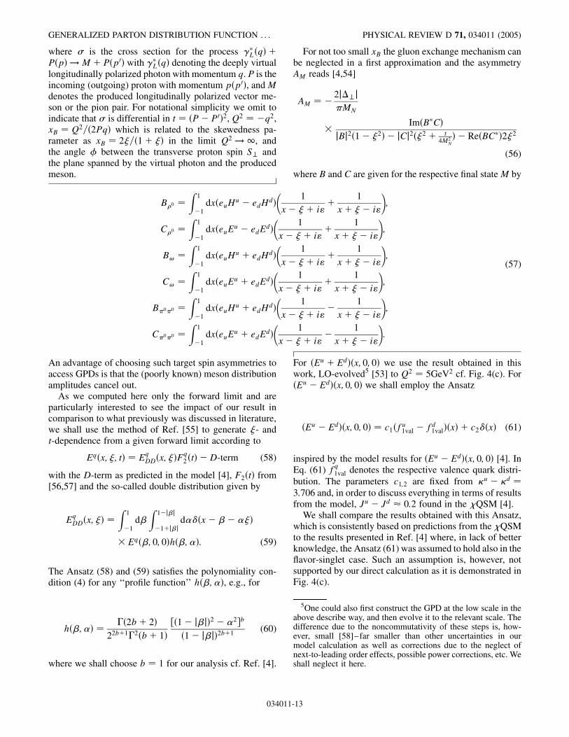
FIG. 5. The transverse spin asymmetry in hard exclusive production of (a) !0, (b) +0, and (c) a 0 pair as functions of xB att �0:5 GeV2 and Q2 5 GeV2.


The GPDHq�x; �; t� is modeled in an analog way on thebasis of the parametrization [59] for fq1 �x� as described inRef. [4].

As can be seen from Fig. 5 the asymmetry has littlesensitivity to the Ansatz used for �Eu � Ed��x; 0; 0� in thecase of !0 or +0 production. We find that the process mostsensitive to �Eu � Ed��x; 0; 0� is the production of a 0

pair. The effect of different Ansatze can clearly be distin-guished. Experiments at HERMES or JLAB could provideinteresting insights. However, for an unambiguous quanti-tative analysis of the data it will be necessary to considersystematically power and next-to-leading ordercorrections.

VIII. SUMMARY AND CONCLUSIONS

We have presented in the framework of the flavor-SU(2)version of the chiral quark-soliton model a study of unpo-larized GPDs, which appear at subleading order in thelarge-Nc limit, namely, the flavor combinations �Eu �Ed��x; �; t� and �Hu �Hd��x; �; t�. For that we generalizedthe methods of Ref. [15] developed to study the leadinglarge-Nc GPDs, i.e., the, respectively, opposite flavorcombinations.

Interestingly, the GPDs �Hu �Hd��x; �; t� and �Eu �Ed��x; �; t� are of the same order in the large-Nc countingbut handled differently in the model. The former appearsalready in leading order, while for the latter one mustinvoke 1=Nc (rotational) corrections to obtain a nonvanish-ing result. Nevertheless they enter the spin sum rule onequal footing, which is satisfied in the model as we dem-onstrated. Furthermore, we have shown that also the sub-leading GPDs satisfy the polynomiality condition, and thatthe coefficients in front of the highest power in � in evenmoments of �Hu �Hd��x; �; t� and �Eu � Ed��x; �; t� areequal to each other up to an opposite sign. Given thedifferent technical handling in the model, the fulfillmentof general requirements where both GPDs are involved is astrong check of the consistency of the approach.

034011

In the chiral quark-soliton modelMQ 2JQ already at alow scale, i.e., the fractions of nucleon momentum and spincarried by quarks and antiquarks are the same. In QCD thisrelation becomes exact in the limit of a large renormaliza-tion scale. Actually this is not a specific prediction of thechiral quark-soliton model, but should hold in any modeldescribing the nucleon consistently in terms of quark andantiquark degrees of freedom, i.e., without gluon degreesof freedom. For such models to be consistentMQ 2JQ 1 must hold. The chiral quark-soliton model fulfills thisrequirement. In the framework of the �QSM the contribu-tion of gluons to the nucleon momentum and angularmomentum is suppressed with respect to the correspondingquark contributions by the small parameter characterizingthe packing fraction of instantons in vacuum [40].

We then focused on the GPD �Eu � Ed��x; �; t� andcomputed numerically its forward limit with a constant(momentum-independent) constituent quark mass M usingthe Pauli-Villars regularization. We found that �Eu �Ed��x; 0; 0� is negative at larger x and sizeable, and positiveat small x, changing the sign at x � 0:2, while �E �u � E �d��x; 0; 0� is always positive and concentrated towardssmaller x. Noteworthy is that in the model in the chirallimit �Eu � Ed��x; 0; 0� is strongly enhanced at small xwith respect to �Hu �Hd��x; 0; 0�. It would be interestingto study in more detail the chiral mechanism responsiblefor that.

On the basis of our results we estimated azimuthalasymmetries in hard exclusive production of vector mesonsand pion pairs from a transversely polarized proton target.We observe that pion pair production is very sensitive to�Eu � Ed��x; �; t�. Data from experiments at HERMES orJLAB on this reaction would be well-suited to distinguishamong different models.

Our work– in particular the demonstration of the con-sistency of the approach–not only increases the faith intothe applicability of the chiral quark-soliton model to thecomputation of GPDs, but also practically paves the way tofurther studies of GPDs in leading and subleading order ofthe large-Nc limit.

-14


ACKNOWLEDGMENTS

We thank Vadim Guzey for help on evolution, and thankMarkus Diehl and Peter Kroll for valuable discussions.This work is partially supported by the Graduierten-Kolleg Bochum-Dortmund and Verbundforschung ofBMBF. A Portuguese-German collaboration grant byGRICES and DAAD is acknowledged. M. V. P. thanks theAlexander von Humboldt-Stiftung for support, FNRS(Belgium) and IISN.

Note added—After this work was finished Ref. [61]appeared, where among others a fit of �Eq � E �q��x; 0; t�to the Pauli form factor was reported. The result ofRef. [61] for �Eu � Ed � E �u � E �d��x; 0; 0� is qualitativelysimilar to the ansatz of Ref. [4] plotted in Fig. 4(c) anddiffers from our result which is negative at all x.

APPENDIX A: MODEL SYMMETRIES

The effective Hamiltonian Heff , Eq. (11), commuteswith the parity operator 4 and the grand-spin operator

K S� L� T (A1)

where S 12)5)

0�, L r� p and T 12 * denote the

single-quark spin, angular momentum and isospin opera-tors, respectively. Thus, the single-quark states are charac-terized by the eigenvalues of 4, K2 and K3 asjni jEn; ;K;K

3i.Consider the unitary matrix G5 given in the standard

representation of Dirac- and flavor-SU(2) matrices byG5 � )2)5*2. It acts as G5)�G�1

5 �)��T andG5*

aG�15 ��*a�T such that in coordinate space the

034011

Hamiltonian (11) is transformed as G5HG�15 HT . This

transformation acts as G5,n�x� , n�x�. The G5 trans-

formation in the effective chiral theory corresponds to timereversal transformation accompanied by a flavor rotation[60]. Using the G5-transformation one finds hmj*ajji �hjj*ajmi and, e.g.,

hmj�1 � )0)3�F�p�G�X�H�p�jji

hjj�1 � )0)3�H��p�G�X�F��p�jmi;

hmj*c�1 � )0)3�F�p�G�X�H�p�jji

�hjj*c�1 � )0)3�H��p�G�X�F��p�jmi:

(A2)

Another useful symmetry of the model is parity 4jmi pmjmi with pm !1 depending on the parity of the state.We obtain, e.g.,

hmj*c�1 � )0)3�F�p�G�X�H�p�jji

pmpjhmj*c�1 � )0)3�H��p�G��X�F��p�jji:

(A3)

APPENDIX B: POLYNOMIALITY

For the discussion of moments the following expressionsfor HE�x; �; t� and EM�x; �; t� are more convenient

HE�x; �; t� �MNNc12I

Z dz0

2 eiz

0xMN

"( Xm; occ

j; all

e�iz0Em �

Xm; all

j; occ

e�iz0Ej

)1

Em � Ejhmj*ajjihjj*a�1 � )0)3�

� exp��iz0p3=2� exp�i�X� exp��iz0p3=2�jmi � iz0X

m; occ

e�iz0Emhmj3�1 � )0)3� exp��iz0p3=2�

� exp�i�X� exp��iz0p3=2�jmi

#; (B1)

EM�x; �; t� iM2

NNc2I

Z dz0

2 eiz

0xMN

"( Xm; occ

j; all

e�iz0Em �

Xm; all

j; occ

e�iz0Ej

)1

Em � Ejhmj*bjjihjj�1 � )0)3� exp��iz0p3=2�

�43ab�a

�2?

exp�i�X� exp��iz0p3=2�jmi � iz0X

m; occ

e�iz0Emhmj*b�1 � )0)3� exp��iz0p3=2�

�43ab�a

�2?

exp�i�X� exp��iz0p3=2�jmi

#: (B2)

If we take out from the double sums the limiting case Em ! Ej and combine it with the respective single sums in (B1) and(B2), then we arrive at the expressions in Eqs. (28) and (29).

-15


1. HE�x; �; t�

In order to demonstrate that at t 0 the moments of HE�x; �; t� are in fact functions of � only, we have to continueanalytically the expression in Eq. (B1) to the unphysical point t 0. For that note that

exp�i�X� X1le0

��i2�MN�le

le!jXjlePle�cosH� (B3)

where cosH X3=jXj and Ple are Legendre polynomials cf. Ref. [17]. Taking moments ofHE�x; �; t� in Eq. (B1) and using(B3) we obtain

M�L�E ��; 0� �

Z 1

�1dxxL�1HE�x; �; t�

�MNNc12IML

N

X1le0

��i2�MN�le

le!

"XL�1

Li0

�L� 1

Li

� XLiJ0

�LiJ

�1

2Li

( Xm; occ

j; all

EL�Li�1m �

Xm; all

j; occ

EL�Li�1j

)

�AEmj

Em � Ej� �L� 1�

XL�2

Li0

�L� 2

Li

� XLiJ0

�LiJ

� Xm; occ

EL�Li�2m

1

2LiBEm

#; (B4)

with

AEmj � hmj*bjjihjj*b�1 � )0)3��p3�JjXjlePle�cosH�

� �p3�Li�Jjmi;

BEm � hmj3�1 � )0)3��p3�JjXjlePle�cosH��p3�Li�Jjmi:

(B5)

Using the G5-symmetry cf. Eq. (A2), we obtain

AEmj � ��1�Lihjj*bjmihmj*b�1 � )0)3�

� �p3�JjXjlePle�cosH��p3�Li�Jjji;

BEm � ��1�Lihmj3�1 � )0)3��p3�JjXjlePle�cosH�

� �p3�Li�Jjmi:

(B6)

Exploring these identities (for the first it is necessary torename under the sum in (B4) m$ j) we see that AEmj andBEm in Eq. (B4) are effectively given by [note that�)0)3�N 1 for even N and )0)3 for odd N]

AEmj hmj*bjjihjj*b�)0)3�Li�p3�JjXjlePle�cosH�

� �p3�Li�Jjmi;

BEm hmj3�)0)3�Li�p3�JjXjlePle�cosH��p3�Li�Jjmi:

(B7)

From parity transformations cf. Eq, (A3), we conclude that

034011

AEmj BEm 0 if le is odd. Thus we observe that only evenpowers in � contribute to the moments. In the next step wedemonstrate that the infinite series in �2 is actually apolynomial.

For that let us first observe that the object *bjjihjj*b

(where summation over b is implied) is invariant underhedgehog rotations. Thus it is practically an irreduciblespherical tensor operator of rank zero with respect tosimultaneous isospin- and space-rotations [17]. So inboth cases, AEmj and BEm, we deal with matrix elements of

the type hmjOjmi, the only difference being the ‘‘replace-ment’’ *bjjihjj*b ! 3 which is irrelevant for our argu-ments. The matrix elements hmjOjmi are nonzero only ifthe operator O is rank zero cf. [17] for details. O is aproduct of pa, )0)3 which have rank 1, and Ple which isrank le, and rank zero operators. O is in general a reducibleoperator which, however, can be decomposed into a sum ofirreducible tensor operators. For our purposes it is impor-tant to find the highest value for le in the Legendre poly-nomial which yields a nonvanishing result for hmjOjmi.The operators pa, which appear Li-times in whateverordering, and operator )0)3, for odd Li, can combine toan operator with maximally rank Li � 1 for odd Li (Li foreven Li). Thus le can have at most rank Li � 1 for odd Li(Li for even Li), otherwise the total operator O cannotreach the needed rank zero. Considering that Li � �L� 1�

we see that the Lth moment of M�L�E is a polynomial with

the highest power �L for even L (�L�1 for odd L). Thus weobtain

-16


M�L�E ��; 0� �

MNNc12IML

N

"XL�1

Li0

�L� 1

Li

� XLiJ0

�LiJ

�1

2Li

XLi�1

le 0

leeven

��i2�MN�le

le!

( Xm; occ

j; all

EL�Li�1m �

Xm; all

j; occ

EL�Li�1j

)AEmj

Em � Ej

� �L� 1�XL�2

Li0

�L� 2

Li

� XLiJ0

�LiJ

�1

2Li

XLi�2

le 2

leeven

��i2�MN�le�2

le!

Xm; occ

EL�Li�2m BEm

#: (B8)

2. EM�x; �; t�

In this case the relevant structure to be continued analytically to t 0 is cf. Ref. [17],

�a?

�2?

exp�i�X� X1le2


le!�pa?; jXjlePle�cosH� : (B9)

With this result we obtain for the moments of EM�x; �; t� at zero t the result

M�L�M ��; 0� �

Z 1

�1dxxL�1EM�x; �; t�

iM2

NNc2IML

N

X1le2


le!

"XL�1

Li0

�L� 1

Li

� XLiJ0

�LiJ

�1

2Li

( Xm; occ

j; all

EL�Li�1m �

Xm; all

j; occ

EL�Li�1j

)

�AMmj

Em � Ej� �L� 1�

XL�2

Li0

�L� 2

Li

� XLiJ0

�LiJ

� Xm; occ

EL�Li�2m

1

2LiBm

#; (B10)

with

AMmj � hmj*bjjihjj�1 � )0)3�

� �p3�J43ab�pa?; jXjlePle�cosH� �p3�Li�Jjmi;

BMm � hmj*b�1 � )0)3��p3�J43ab�pa?; jXjlePle�cosH�

� �p3�Li�Jjmi: (B11)

From the G5-symmetry cf. Eq. (A2), we obtain

AMmj hmj*bjjihjj�)0)3�Li�1�p3�J43ab�pa?; jXjle

� Ple�cosH� �p3�Li�Jjmi;

BMm hmj*b�)0)3�Li�1�p3�J43ab�pa?; jXjlePle�cosH�

� �p3�Li�Jjmi:

(B12)

From parity transformations cf. Eq. (A3), it follows thatAMmj and BMm are zero if le is odd. Thus we observe againthat only even powers in � contribute to the moments.

In order to demonstrate that the infinite series in evenpowers of � is actually a polynomial, let us consider firstthe double sum contribution in Eq. (B10). We deal with thematrix elements AMmj which are of the type hmj*ajji�

034011

hjjOajmi. The operator *a is an irreducible spherical tensoroperator of rank one with respect to simultaneous isospin-and space- (hedgehog-) rotations [17]. Thus only certaintransitions hmj*ajji between the states jmi and jji arenonzero. In order for the entire expression for AMmj to be

nonzero the same transitions must appear also in the piecehjjOajmi, thus the operator Oa must be rank 1, too.

The operators *a, pa, )0)3 and Ple , which in our contextare relevant for the rank counting, can combine to anoperator with maximally rank Li � 2 for even Li (Li � 1for odd Li). Thus le can be at most Li � 3 for even Li (Li �2 for odd Li), otherwise the total operator Oa cannot reachthe needed rank 1. However, le must be even, thus le ��Li � 2� for even Li (Li � 1 for odd Li). Finally Li ��L� 1�. Therefore the double sum contribution to theLth moment ofM�L�

M is a polynomial with the highest power�L�2 for even L (�L�1 for odd L).BMm in Eq. (B12) is zero unless the operators (jXj, *a, the

Li � 1 operators pa, Ple , and )0)3 if Li is odd) combine toa rank 0 operator. One obtains the same restriction for themaximal value of le in terms of Li as above, however, inthis case Li � �L� 2�. Thus, we finally obtain [with AMmj,BMm given in Eq. (B12)]

-17


M�L�M ��; 0�

iM2NNc

2IMLN

"XL�1

Li0

�L� 1

Li

� XLiJ0

�LiJ

�1

2Li

XLi�2

le 2

leeven


le!

( Xm; occ

j; all

EL�Li�1m �

Xm; all

j; occ

EL�Li�1j

)AMmj

Em � Ej

� �L� 1�XL�2

Li0

�L� 2

Li

� XLiJ0

�LiJ

�1

2Li

XLi�2

le 2

leeven


le!

Xm; occ

EL�Li�2m BMm

#: (B13)

We know that �Hu �Hd��x; �; t� satisfies polynomiality and that its even moments L are polynomials of degree L [17].Here we observe that even moments L of EM�x:�; t� are polynomials of degree �L� 2�. Since EM�x; �; t� is the sum of�Eu � Ed��x; �; t� and �Hu �Hd��x; �; t� this means that the moments of �Eu � Ed��x; �; t� also satisfy polynomiality andthat the coefficients of the highest power �L of even moments satisfy the relation (5).

APPENDIX C: PROOF OF THE SPIN SUM RULE

The model expression for the second moment of EM�x; �; t� is given by (B13) for L 2. By observing that�pa?; X

2P2�cosH� iXa? we obtain

M�2�M ��; 0� �

Nc4I

" Xm; occj; all

�Em � Ej�hmj*bjjihjj�)0)3�43abXa?jmi

Em � Ej�

Xm; occj; non

2hmj*bjjihjjp343abXa?jmiEm � Ej

#: (C1)

Using the following identity, where we explore the equa-tions of motion in the model,

hjj�Em � Ej�)0)3Xj?jmi hjjfH;)0)3Xj?gjmi

hjj�2p3Xj? � i)j)3�jmi

(C2)

we obtain

M�2�M ��; 0�

Nc2I

Xm; occ

j; non

1

Em � Ej�hmj*3jjihjj)0)3)5jmi

� 2hmj*3jjihjj43abXapbjmi : (C3)

In Eq. (C3) we identify the model expressions for the spinSQ and angular momentum LQ contribution of quarks andantiquarks to the spin of the nucleon SN

034011

SQ �Nc2I

Xm; occ

j; non

1

Em � Ejhmj*3jjihjj)0)3)5jmi

1

2g�0�A ;

LQ �NcI

Xm; occ

j; non

1

Em � Ejhmj*3jjihjj43jkXjpkjmi;

(C4)

where g�0�A denotes the isosinglet axial coupling constant.The operators in (C3) can be added according to Eq. (A1)

1

2)0)3)5 � 43jkXjp3 S3 � L3 K3 � T3: (C5)

Noting that in Eq. (C3) the matrix elements hjjK3jmi K3j 3jm vanish we obtain

M�2�M ��; 0� � 2SQ � 2LQ

Nc4I

Xm; occ

j; non

1

Ej � Emhmj*3jjihjj*3jmi 1:

(C6)

-18


[1] D. Muller, D. Robaschik, B. Geyer, F. M. Dittes, and J.Horejsi, Fortschr. Phys. 42, 101 (1994).A. V. Radyushkin,Phys. Lett. B 385, 333 (1996); Phys. Rev. D 56, 5524(1997); X. D. Ji, Phys. Rev. D 55, 7114 (1997); J. C.Collins, L. Frankfurt, and M. Strikman, Phys. Rev. D56, 2982 (1997).

[2] X. D. Ji, J. Phys. G 24, 1181 (1998).[3] A. V. Radyushkin in At the Frontier of Particle Physics/

Handbook of QCD, edited by M. Shifman (WorldScientific, Singapore, 2001).

[4] K. Goeke, M. V. Polyakov, and M. Vanderhaeghen, Prog.Part. Nucl. Phys. 47, 401 (2001).

[5] M. Diehl, Phys. Rep. 388, 41 (2003).[6] X. D. Ji, Phys. Rev. Lett. 78, 610 (1997).[7] J. P. Ralston and B. Pire, Phys. Rev. D 66, 111501 (2002);

M. Burkardt, Int. J. Mod. Phys. A 18, 173 (2003).[8] M. V. Polyakov, Phys. Lett. B 555, 57 (2003).[9] For an overview see: M. Vanderhaeghen, Nucl. Phys.

A711, 109 (2002).[10] HERMES Collaboration, A. Airapetian et al., Phys. Rev.

Lett. 87, 182001 (2001); CLAS Collaboration, S.Stepanyan et al., Phys. Rev. Lett. 87, 182002 (2001); H1Collaboration, C. Adloff et al., Phys. Lett. B 517, 47(2001); ZEUS Collaboration, S. Chekanov et al., Phys.Lett. B 573, 46 (2003).

[11] M. Vanderhaeghen, P. A. Guichon, and M. Guidal, Phys.Rev. D 60, 094017 (1999); N. Kivel, M. V. Polyakov, andM. Vanderhaeghen, Phys. Rev. D 63, 114014 (2001); A. V.Belitsky, D. Muller, A. Kirchner, and A. Schafer, Phys.Rev. D 64, 116002 (2001); V. A. Korotkov and W. D.Nowak, Eur. Phys. J. C 23, 455 (2002); A. V. Belitsky,D. Muller, and A. Kirchner, Nucl. Phys. B629, 323 (2002);A. Freund and M. F. McDermott, Phys. Rev. D 65, 074008(2002); Eur. Phys. J. C 23, 651 (2002); A. Freund, M.McDermott, and M. Strikman, Phys. Rev. D 67, 036001(2003).A. Kirchner and D. Muller, Eur. Phys. J. C 32, 347(2003).

[12] M. V. Polyakov and A. G. Shuvaev, hep-ph/0207153.[13] P. V. Pobylitsa, Phys. Rev. D 65, 077504 (2002); 65,

114015 (2002); 66, 094002 (2002); 67, 034009 (2003);67, 094012 (2003); 70, 034004 (2004).

[14] X. D. Ji, W. Melnitchouk, and X. Song, Phys. Rev. D 56,5511 (1997).

[15] V. Y. Petrov, P. V. Pobylitsa, M. V. Polyakov, I. Bornig, K.Goeke, and C. Weiss, Phys. Rev. D 57, 4325 (1998).

[16] M. Penttinen, M. V. Polyakov, and K. Goeke, Phys. Rev. D62, 014024 (2000).

[17] P. Schweitzer, S. Boffi, and M. Radici, Phys. Rev. D 66,114004 (2002); Nucl. Phys. A711, 207 (2002); P.Schweitzer, M. Colli, and S. Boffi, Phys. Rev. D 67,114022 (2003).

[18] A. Mukherjee and M. Vanderhaeghen, Phys. Lett. B 542,245 (2002);Phys. Rev. D 67, 085020 (2003).

[19] S. Boffi, B. Pasquini, and M. Traini, Nucl. Phys. B649,243 (2003); B680, 147 (2004).

[20] A. Radyushkin, Ann. Phys. (Berlin) 13, 718 (2004).[21] M. Vanderhaeghen, Ann. Phys. (Berlin) 13, 740 (2004).[22] D. I. Diakonov and V. Y. Petrov, Pis’ma Zh. Eksp. Teor.

Fiz. 43, 57 ( 1986) [JETP Lett. 43, 75 (1986)].[23] D. I. Diakonov, V. Y. Petrov, and P. V. Pobylitsa, Nucl.

Phys. B306, 809 (1988).D. I. Diakonov, V. Y. Petrov, and

034011

M. Praszałowicz, Nucl. Phys. B323, 53 (1989).[24] C. V. Christov, A. Z. Gorski, K. Goeke, and P. V. Pobylitsa,

Nucl. Phys. A592, 513 (1995).[25] C. V. Christov et al., Prog. Part. Nucl. Phys. 37, 91 (1996).[26] D. I. Diakonov et al., Nucl. Phys. B480, 341 (1996).[27] P. V. Pobylitsa and M. V. Polyakov, Phys. Lett. B 389, 350

(1996).[28] D. Diakonov, V. Y. Petrov, P. V. Pobylitsa, M. V. Polyakov,

and C. Weiss, Phys. Rev. D 56, 4069 (1997).[29] C. Weiss and K. Goeke, hep-ph/9712447.[30] P. V. Pobylitsa et al., Phys. Rev. D 59, 034024 (1999).[31] D. Diakonov, V. Y. Petrov, P. V. Pobylitsa, M. V. Polyakov,

and C. Weiss, Phys. Rev. D 58, 038502 (1998).[32] M. Wakamatsu and T. Kubota, Phys. Rev. D 60, 034020

(1999).[33] K. Goeke et al., Acta Phys. Pol. B 32, 1201 (2001).[34] P. Schweitzer et al., Phys. Rev. D 64, 034013 (2001).[35] M. V. Polyakov and C. Weiss, Phys. Rev. D 60, 114017

(1999); O. V. Teryaev, Phys. Lett. B 510, 125 (2001).[36] D. I. Diakonov and M. I. Eides, Pis’ma Zh. Eksp. Teor. Fiz.

38, 358 (1983) [JETP Lett. 38, 433 (1983)]; A. Dhar, R.Shankar, and S. R. Wadia, Phys. Rev. D 31, 3256(1985).

[37] D. I. Diakonov and V. Y. Petrov, Nucl. Phys. B272, 457(1986).

[38] D. I. Diakonov and V. Y. Petrov, Nucl. Phys. B245, 259(1984).

[39] E. Witten, Nucl. Phys. B223, 433 (1983).[40] D. Diakonov, M. V. Polyakov, and C. Weiss, Nucl. Phys.

B461, 539 (1996).[41] J. Balla, M. V. Polyakov, and C. Weiss, Nucl. Phys. B510,

327 (1998).B. Dressler and M. V. Polyakov, Phys. Rev. D61, 097501 (2000).

[42] See Sec. 3 of Ref. [4]; Cf. also P. V. Pobylitsa and M. V.Polyakov, Phys. Rev. D 62, 097502 (2000); P. V. Pobylitsa,hep-ph/0203268; A. V. Efremov, K. Goeke, and P. V.Pobylitsa, Phys. Lett. B 488, 182 (2000).

[43] X. D. Ji, J. Tang, and P. Hoodbhoy, Phys. Rev. Lett. 76,740 (1996).

[44] P. Hagler and A. Schafer, Phys. Lett. B 430, 179 (1998);A. Harindranath and R. Kundu, Phys. Rev. D 59, 116013(1999); P. Hoodbhoy, X. D. Ji, and W. Lu, Phys. Rev. D 59,014013 (1999).

[45] M. Wakamatsu and T. Watabe, Phys. Rev. D 62, 054009(2000).

[46] O. V. Teryaev, hep-ph/9904376; hep-ph/9803403.[47] A. Freund, Eur. Phys. J. C 31, 203 (2003).[48] M. Wakamatsu and H. Yoshiki, Nucl. Phys. A524, 561

(1991).[49] A. Freund and L. M. Sehgal, Phys. Lett. B 341, 90 (1994);

S. D. Bass, S. J. Brodsky, and I. Schmidt, Phys. Lett. B437, 417 (1998).

[50] S. Kahana and G. Ripka, Nucl. Phys. A429, 462 (1984).[51] T. Kubota, M. Wakamatsu, and T. Watabe, Phys. Rev. D

60, 014016 (1999).[52] M. Gluck, E. Reya, and A. Vogt, Eur. Phys. J. C 5, 461

(1998);Z. Phys. C 67, 433 (1995).[53] We used the QCD evolution program of QCDNUM avail-

able at http://www.nikhef.nl/ h24/qcdnum.[54] B. Lehmann-Dronke, A. Schafer, M. V. Polyakov, and K.

Goeke, Phys. Rev. D 63, 114001 (2001); B. Lehmann-

-19


Dronke, P. V. Pobylitsa, M. V. Polyakov, A. Schafer, andK. Goeke, Phys. Lett. B 475, 147 (2000).

[55] A. V. Radyushkin, Phys. Rev. D 59, 014030 (1999).[56] E. J. Brash, A. Kozlov, S. Li, and G. M. Huber, Phys. Rev.

C 65, 051001 (2002).[57] P. E. Bosted, Phys. Rev. C 51, 409 (1995).[58] I. V. Musatov and A. V. Radyushkin, Phys. Rev. D 61,

034011

074027 (2000).[59] A. D. Martin, R. G. Roberts, W. J. Stirling, and R. S.

Thorne, Eur. Phys. J. C 28, 455 (2003).[60] P. V. Pobylitsa, hep-ph/0212027.[61] M. Diehl, T. Feldmann, R. Jakob, and P. Kroll, hep-ph/

0408173.

-20

Documents

of the nucleon in the chiral quark soliton model