Simulation of Hydrodynamic Slug Formation in Multiphase Flowlines and 

Separation Devices 

Dissertation Submitted to the Department of Mineral Resources and Petroleum Engineering and the Committee on Graduate Studies of Montanuniversität Leoben, Austria

In Partial Fulfilment of the Requirements for the Degree of Doktor der Montanistischen Wissenschaften

Advisor A.o. Univ.Prof. Dipl.­Ing. Dr.  

W. Brandstätter 

Written by Adel Mohamed Salem Ragab, 

 M. Sc. Eng. 

Leoben – Nov. 2008

Simulation of Hydrodynamic Slug Formation in Multiphase Flowlines and Separation Devices Doctoral Thesis

By Adel M. S. Ragab, M. Sc.

Page:i

Dedication

To my parents Mohamed and Fatima, to my wife Abir and our two

sons: Mohamed and Mohand

Page:ii

Affidavit

I declare in lieu of oath, that I wrote this thesis and performed the associated

research myself, using only literature cited in this volume.

Adel Ragab, M. Sc. Eng.

Leoben, November 2008

Page:iii

Abstract

Multiphase flow phenomena are encountered in all disciplines of petroleum engineering industry; drilling, production, reservoir, processes, and transportation operation. Since the crude oil production pipelines follow normal hilly terrain variations including horizontal, uphill, and downhill sections, it is possible to find several types of flow regimes at the same time at different position along the pipeline. Most of the possible flow regimes are not dangerous except slug flow. Therefore, this flow regime remains a major and expensive headache for oil produces. It causes poor crude oil separation, limit production, and at the end it may lead to cease production. In this study, the fluid dynamics of gas liquid slug flows in horizontal, inclined, and hilly terrain pipelines are modeled using multi-dimensional Computational Fluid Dynamics (CFD) codes. The Volume of Fluid Model (VOF) as an interface tracking technique, is developed to predict, visualize and monitor the flow regime. The first part of the thesis is consisting of a study the flow regimes in small diameter pipelines and their characteristics. Therefore, a set of simulation runs was performed to compute flow patterns in horizontal and inclined gas-liquid pipelines. The first set of runs was done using a horizontal pipe and the results were verified against experimental work. The study covers a wide range of fluid flow rates. The slug flow characteristics have been calculated, and new relations between the superficial liquid velocity and liquid hold up have been derived. The second set of runs was conducted for a pipeline with inclination angels +5°. The effect of pipe inclination on the flow regime was studied and the flow patterns, liquid holdup and pressure drop have been computed. The second part of the work dealt with the complex and multi-dimensional nature of slug flow. It includes simulation of a full scale field pipeline from OMV-Austria By CFD-VOF technique. The transient flow behaviour occurring in a pipeline with two different diameters has been simulated. Since the pipeline under consideration is nearly 2 Km long, the corresponding computational model would involve grid cells with very large aspect ratios which invariably would lead to solution instabilities in the CFD analysis. To overcome this problem, the pipeline was sub-divided into different sections, and each section was investigated separately. Then, the whole length was simulated and complete investigations have been presented in terms of slug flow characteristics (Slug Velocity, Pressure drop, slug frequency, and holdup). The ultimate aim of this research work was to gain a deeper understanding of multiphase flow phenomena in pipelines and to guidelines to improve the design of pipelines and downstream facilities

Page:iv

Kurzfassung

Mehrphasenströmungen treten in praktisch allen Bereichen der Erdölindustrie auf. Insbesondere im Produktionsbereich sind mehrphasige Strömungsphänomene anzutreffen. Da Pipelines normalerweise im hügeligen Terrain verlegt werden und horizontale, aufwärts und abwärts gerichtete Leitungsabschnitte vorhanden sein können, führt dies dazu, dass verschiedene Arten von Strömungsregimen innerhalb einer Pipeline auftreten können, wobei sogenannte „Slug Flow Phänomene“ besonders kritisch sein können. Diese können eine schlechte Trennung der einzelnen Phasen des Rohöls oder Produktionsbeschränkungen bewirken und im Extremfall zum Stillstand der Produktion führen. In der vorliegenden Arbeit wird die Strömungsdynamik von Gas/Flüssig Slug Flows in horizontalen und geneigten Pipelines detailliert untersucht. Dabei wird mit Hilfe moderner Computational Fluid Dynamics (CFD) Werkzeuge und dem Volume-of-Fluid (VoF) Modell die Vorhersage, das Monitoring und die Visualisierung dieses Flow Regimes detailliert berechnet. Der erste Teil der Arbeit beinhaltet eine Darstellung aller möglichen Flow Regime und deren charakteristischen Eigenschaften in Pipelines von geringem Durchmesser. In diesem Zusammenhang wurde eine Vielzahl von Simulationsrechnungen in horizontalen und geneigten Gas/Flüssigkeitspipelines durchgeführt. Darüber hinaus wurde soweit als möglich versucht, die Ergebnisse anhand von experimentellen Daten, die der Literatur entnommen wurden, zu verifizieren. Eine neue Korrelation zwischen „Superficial Liquid Velocity“ und „Liquid Hold Up“ zur Charakterisierung von Slug Flow Phänomenen in horizontalen Rohren konnte hergeleitet werden. Der Effekt der Rohrneigung auf die Ausbildung verschiedener Flow Regimes wurde untersucht und Strömungseigenschaften, „Liquid Hold Up“ und Druckabfall wurden berechnet. Der zweite Teil der Arbeit konzentriert sich auf die komplexe und mehrdimensionale Natur von Slug Flow Phänomenen. Darin werden mit Hilfe der entwickelten Simulationswerkzeuge Teile des Produktionsfeldes „Matzen VI“ der OMV AG im Raum Gänserndorf analysiert. Der betrachtete Pipeline Sektor ist annähernd 2 Kilometer lang und es war daher nicht möglich, ein globales Berechnungsmodell für diesen Abschnitt zu erstellen, da das numerische Berechnungsgitter Berechnungszellen mit extremen Teilungsverhältnissen enthalten würde und damit das Auftreten von Instabilitäten im Berechnungsverlauf unvermeidbar wäre. Um dies zu vermeiden, wurde daher die Pipeline in verschiedene Sektionen unterteilt, und jeder Abschnitt einzeln untersucht. Abschließend wurde auch ein längerer Sektor analysiert und es werden die Ergebnisse betreffend Slug Velocities, Slug Frequencies, Liquid Hold Up und Druckabfall diskutiert. Vorrangiges Ziel der Arbeit war es, ein tieferes Verständnis von komplexen Mehrphasenströmungsphänomenen in Pipelines zu erhalten, und Richtlinien für das effiziente Design von Pipelines und Downstream Facilities zu erstellen.

Page:v

Acknowledgements

I would like to express my gratitude to my supervisor Prof. W. Brandstätter for giving me the opportunity to carry out the research into the fascinating subject of multiphase flow modeling in oil field industry. I like to thank him for his perfect guidance, the fruitful discussions, his daily supervision, his continuous supports throughout these years in each in every thing, and constant patience throughout performing all of these research works. In addition, it gives me a great pleasure to thank him for his social part with me. I would like to convey my appreciation to Prof. G. Ruthammer, the professor of Petroleum Production Engineering in petroleum Institute of Leoben University for his helpful discussion and opinions. I would like to thank him also for his careful revision and reading the OMV report. I wish to express my special thanks to Prof. H. Hofstätter, head of Petroleum Production Chair in Leoben University for his support. I am greatly indebted to Prof. Dr. S. Shalaby for his continuous support. He has provided me with much encouragement and support whenever I needed them most. Grateful acknowledgements are strongly expressed to all the members of the team of Prof. Brandstätter in the university and his company (ICE) for their support and help. I also want to give my thanks to the secretary of the petroleum production Miss. Irene Jauck and the secretary of my supervisor in his company (ICE) Miss. Andrea Kreuzig for her encourage and support whenever needed. I strongly wish to express my great appreciation to ÖAD Austria and ÖAD-Leoben branch, especially Miss. D. Holzapfel and Miss. N. Juritsch for their help and support throughout the whole period of the scholarship and their efforts to solve all the problems i met either educational or social. Finally, my profound gratitude is dedicated to my family (my wife Eng. Abir Amer, and our children Mohamed and Mohand) for their understanding and wholehearted support they have given to me.

Page:vi

Communications arising from this thesis The work described in this thesis has been presented as follows: Published Journal Papers: March 2008

Adel Ragab, W. Brandstätter and S. Shalaby: “CFD-Simulation of Multiphase Flows in Horizontal and Inclined Pipelines,” Oil and Gas European Magazine, Oil Gas European Magazine (International Edition of Erdöl Erdgas Kohle), Pages 34-40, Vol. 34, March 1/2008.

Dec. 2008

Adel Ragab, W. Brandstätter and S. Shalaby: “Numerical Simulation of Slug Flow Phenomena in Horizontal and Inclined Pipelines,” Oil and Gas European Magazine (International Edition of Erdöl Erdgas Kohle), accepted for publication in Vol. 4 Dec. 2008.

Conference Papers: Oct. 2007 W. Brandstätter, Adel Ragab and S. Shalaby: “Modeling of Two-Phase Flow and Slug

Flow Characteristics in Horizontal/Inclined Pipelines using CFD,” Presented at SPE Romanian Conference -150 Years of the Romanian Petroleum Industry, Tradition & challenges, held in Athénée Hilton Hotel-Bucharest 14-17 Oct. 2007. (http://romania.spe.org), the proceeding in form of CD-ROM.

May 2008 Adel Ragab, W. Brandstätter and S. Shalaby: “Multiphase Flows in Horizontal and Inclined Pipelines by CFD Simulations,” Presented at the 5th Mediterranean Offshore Conference and Exhibition 2008 (MOC2008), Alexandria, Egypt, 20-22 May 2008. (The proceeding in a form of CD-ROM).

June 2008 Adel Ragab, W. Brandstätter, G. Ruthammer and S. Shalaby: “CFD-Analysis of Terrain-Induced Slug Flow Regimes in Multiphase Pipeline Systems,” Presented at the 6th International Conference on CFD in Oil & Gas, Metallurgical and Process Industries, SINTEF/NTNU, Trondheim, Norway, 10-12 June, 2008. (The proceeding in a form of CD-ROM).

Sept.2008 Adel Ragab, W. Brandstätter, G. Ruthammer and S. Shalaby: “Analysis of Multiphase Production through Hilly Terrain Pipelines in Matzen Field – Austria by CFD,” SPE Paper 115355-PP, Presented at the 2008 SPE Annual Conference and Exhibition held in Denver, Colorado, USA, 21-24 September 2008.

Oct.2008 Adel Ragab, W. Brandstätter, G. Ruthammer and S. Shalaby: “CFD-Numerical Analysis of Multiphase Production through Hilly Terrain Pipelines in Matzen Field – Austria,” SPE 115355-MS, Presented at the 2008 SPE Asia Pacific Oil & Gas Conference and Exhibition held in Perth, Australia, 20-22 Oct. 2008.

Scientific Presentations and Reports: 2006 Adel Ragab, W. Brandstätter, and G. Ruthammer: “CFD Capability to Simulate Multiphase

Flow in Pipes, Risers, and Separators” Presented at Ganzendorf, OMV-Austria on Nov. 31, 2006.

Page:vii

2007 Adel Ragab, W. Brandstätter, and G. Ruthammer: “Transient Hydraulic Analysis Matzen

VI- (CFD-FLUENT)” Presented at OMV Ganzendorf, Vienna on June 15, 2007.

2007 Adel Ragab, W. Brandstätter, and S. Shalaby: “Scientific Report: Summaries the research works along the two-year of OÄD scholarship (Dec.2005-Dec. 2007) in Chair of Petroleum Production and Processing, Petroleum Institute, University of Leoben, 19 Nov. 2007.

Table of Contents

Page:ix

TABLE OF CONTENTS

CHAPTER I Introduction

1.1 Overview................................................................................................................................11.2 Background............................................................................................................................11.3 Statement of the Problem......................................................................................................21.4 Thesis Objectives ..................................................................................................................31.5 Thesis Outlines ......................................................................................................................31.6 References..............................................................................................................................5

CHAPTER II

Historical Review of Multiphase Fluid Flow in Pipelines

2.1 Introduction............................................................................................................................62.2 Single Phase Flow .................................................................................................................62.3 Multiphase Flow....................................................................................................................8

2.3.1 Background of Multiphase Flow Calculations.............................................................82.3.2 Empirical Methods for Multiphase Flow .....................................................................92.3.3 Mechanistic Models for Multiphase Flow..................................................................13

2.3.3.1 Physical Description of the Flow Patterns ..........................................................132.3.3.2 Flow Pattern Identifications and Transitions Models.........................................14

2.3.3.2.1 Stratified Flow Model ...................................................................................162.3.3.2.1.1 Transition between Smooth Stratified to Stratified Wavy Flow.........172.3.3.2.1.2 Transition from Stratified to Non-Stratified Flow ...............................18

2.3.3.2.2 Intermittent Flow Modeling..........................................................................182.3.3.2.2.1 Transition of Intermittent to Annular Flow Regime ............................202.3.3.2.2.2 Transition of Intermittent to Dispersed Flow Regime .........................20

2.3.3.2.3 Annular Flow Modeling................................................................................212.3.3.2.3.1 Annular Flow Transition to Intermittent Flow.....................................22

2.3.3.2.4 Dispersed Flow Modeling.............................................................................222.3.3.2.4.1 Transition of Bubble Flow to Intermittent Flow ..................................23

2.4 Nomenclature.......................................................................................................................232.5 References............................................................................................................................24

CHAPTER III

Slug Flow Characteristics

3.1 Introduction..........................................................................................................................293.2 Slug Flow Mechanisms and Problems ...............................................................................293.3 Slugging Types....................................................................................................................30

3.3.1 Hydrodynamic Slugging..............................................................................................303.3.2 Terrain-Induced Slugging............................................................................................303.3.3 Severe Slugging ...........................................................................................................30

3.4 Slug Mitigation and Prevention Methods ..........................................................................323.5 Slug Flow Characteristics ...................................................................................................33

Table of Contents

Page:x

3.5.1 Slug Length ..................................................................................................................343.5.2 Slug Frequency.............................................................................................................363.5.3 Slug Holdup..................................................................................................................383.5.4 Slug Velocity................................................................................................................40

3.6 Nomenclature.......................................................................................................................413.7 References............................................................................................................................42

CHAPTER IV

Computational Fluid Dynamics for Multiphase Flow The Volume of Fluid Method (VOF)

4.1 Introduction..........................................................................................................................464.2 General Governing Equations ............................................................................................46

4.2.1 Mass Balance Equation ...............................................................................................464.2.2 Momentum Equation ...................................................................................................474.2.3 Energy Equation...........................................................................................................47

4.3 Constitutive Relationships ..................................................................................................484.3.1 Basic Constitutive Relations .......................................................................................48

4.4 Free-Surface Flows .............................................................................................................484.4.1 Front-Tracking Approach............................................................................................494.4.2 Front-Capturing Approach ..........................................................................................50

4.5 Turbulence Modelling.........................................................................................................504.5.1 Reynolds Averaged Navier-Stokes (RANS) Equations ............................................514.5.2 The Standard κ-ε Model ..............................................................................................53

4.6 Source Terms.......................................................................................................................544.6.1 Gravity ..........................................................................................................................544.6.2 Surface Tension............................................................................................................55

4.7 Physical Properties ..............................................................................................................574.7.1 Density..........................................................................................................................574.7.2 Viscosity .......................................................................................................................584.7.3 Surface Tension............................................................................................................58

4.8 Boundary and Initial Conditions ........................................................................................584.8.1 Mathematical Classification ........................................................................................594.8.2 Boundary Conditions (BC)..........................................................................................594.8.3 Initial Conditions..........................................................................................................59

4.9 Numerical Method...............................................................................................................604.9.1 Mathematical Model ....................................................................................................604.9.2 Discretization Principles..............................................................................................61

4.9.2.1 Numerical Grid .....................................................................................................634.9.2.2 Calculation of Integrals ........................................................................................634.9.2.3 Spatial Variation ...................................................................................................644.9.2.4 Integration in Time ...............................................................................................65

4.10 Algebraic Equation Systems Derivation..........................................................................654.10.1 Convective Fluxes: High-Resolution Interface Capturing Scheme........................654.10.2 Resulting Algebraic Equation ...................................................................................674.10.3 Calculation of Pressure..............................................................................................68

4.11 Nomenclature.....................................................................................................................704.12 References..........................................................................................................................71

Table of Contents

Page:xi

CHAPTER V Numerical Simulation of Two Phase Flow Phenomena in Horizontal and

Inclined Pipes Stratified & Slug Flow Characterizations

5.1 Introduction..........................................................................................................................725.2 Pipeline Geometries and Boundary Conditions ................................................................73

5.2.1 Numerical Simulation of Horizontal Multiphase Flow .............................................745.2.1.1 Horizontal Flow Pattern Identification................................................................745.2.1.2 Stratified Flow Analysis.......................................................................................77

5.2.1.2.1 Effect of Phase Velocity on the Pressure Drop ...........................................775.2.1.2.2 Phase Velocity versus Minimum Equilibrium Liquid Level ......................78

5.2.1.3 Slug Flow Analysis...............................................................................................795.2.1.3.1 Impact of Phase Velocity on Holdup ...........................................................79

5.2.1.3.1.1 Impact of Liquid Velocity on Holdup Variations ................................805.2.1.3.1.2 Impact of Gas Velocity on Liquid Holdup ...........................................805.2.1.3.1.3 Impact of Mixture Velocity ...................................................................80

5.2.1.3.2 Liquid Film Level of Slug Unit ....................................................................835.2.1.3.3 Slug Transitional Velocity ............................................................................845.2.1.3.4 Slug Length....................................................................................................875.2.1.3.5 Pressure Drop of Slug Flow Regime............................................................88

5.2.1.3.5.1 The Pressure Loss at Constant Liquid Velocity ...................................885.2.1.3.5.2 The Pressure Loss at Constant Gas Velocity........................................89

5.2.2 Numerical Simulation of Inclined Multiphase Flow .................................................925.2.2.1 Inclined Flow Pattern Identification ....................................................................925.2.2.2 Impact of Phase Velocity on Holdup...................................................................93

5.2.2.2.1 Impact of Liquid Velocity on Holdup Variations........................................935.2.2.2.2 Impact of Gas Velocity on Liquid Holdup ..................................................945.2.2.2.3 Impact of Mixture Velocity ..........................................................................96

5.2.2.3 Slug Transitional Velocity ...................................................................................965.2.2.4 Slug Flow Frequency............................................................................................975.2.2.5 Pressure Drop in Slug Flow Regime ...................................................................99

5.2.2.5.1 The Pressure Loss at Constant Liquid Velocity ..........................................995.2.2.5.2 The Pressure Loss at Constant Gas Velocity ...............................................99

5.2.3 Horizontal versus Inclined Two Phase Flow............................................................1015.2.3.1 Slug Velocity.......................................................................................................1025.2.3.2 Slug Length .........................................................................................................1035.2.3.3 Pressure Drop......................................................................................................103

5.3 Conclusions........................................................................................................................1045.4 Nomenclature.....................................................................................................................1045.5 References..........................................................................................................................104

CHAPTER VI

Matzen New Flow Assurance

6.1 The Problem: Project “Matzen Neu” ....................................................................................1076.2 Mechanical Solutions.............................................................................................................107

6.2.1 Flow Regime Prediction .................................................................................................1076.2.2 Liquid Hold up Calculations ..........................................................................................109

Table of Contents

Page:xii

6.2.3 Slug Characteristics ........................................................................................................1106.2.3.1 Slug Length and Volume Calculations...................................................................1106.2.3.2 Slug Velocity Calculations......................................................................................1116.2.3.3 Slug Frequency Calculations ..................................................................................1116.2.3.4 Pressure Drop Calculations.....................................................................................111

6.2.3.4.1 Pressure Drop ΔP-DN400 ................................................................................1126.2.3.4.2 Pressure Drop ΔP-DN450 ................................................................................112

6.3 Numerical Analysis ................................................................................................................1126.3.1 Boundary Conditions and Pipe Geometry.....................................................................1126.3.2 Simulation Results ..........................................................................................................115

6.3.2.1 First Pipe Section Simulations................................................................................1156.3.2.2 Second Pipe Section Simulations ...........................................................................1246.3.2.3 Comparison First and Second Scenario..................................................................1296.3.2.4 Long Section Pipeline of Matzen VI ......................................................................132

6.3.2.3.1 Liquid Holdup...................................................................................................1386.3.2.3.2 Transient Velocity Monitoring ........................................................................1396.3.2.3.3 Slug Length and Slug Volume Calculations...................................................1416.3.2.3.4 Slug Frequency Calculations ...........................................................................1416.3.2.3.5 Pressure Drop in the Pipeline Matzen VI........................................................142

6.4 Conclusions.............................................................................................................................1456.5 Nomenclature..........................................................................................................................1456.6 References...............................................................................................................................146

Appendix 6-A: Graphical Solution of Multiphase Flow in Matzen VI.........................................157Appendix 6-B: Details of Liquid Holdup Calculations..................................................................159

I. Lockhart and Martinelli ....................................................................................................159II. Brown Approach .............................................................................................................160III. Eaton Approach-Liquid Holdup....................................................................................161IV. Abdul-Majeed Approach...............................................................................................162V. Mukherjee-Brill Correlation ...........................................................................................162VI. Minami and Brill............................................................................................................163VII. Beggs and Brill Correlation .........................................................................................163

Appendix 6-C: Slug Characteristics Calculations ..........................................................................164

C1: Slug Length:...........................................................................................................................164C1-1 Brill et al. Equation:........................................................................................................164C1-2 Norris L. Equation: .........................................................................................................164C1-3 Brill-Scott Equation: .......................................................................................................164C1-4 Hill-Wood Equation:.......................................................................................................164

C2: Slug Transitional Velocity ....................................................................................................165C3: Slug Frequency ......................................................................................................................165

Appendix 6-D: Beggs and Brill Correlation ...................................................................................167

CHAPTER VII Conclusions and Future Developments

7.1 Conclusions.................................................................................................................................1717.2 Future Developments and Recommendations ..........................................................................172

List of Figures

Page:xiii

LIST OF FIGURES

Figure 2-1: Schematic of a simple 1D single phase flow..............................................................7Figure 2-2: Flow patterns in horizontal pipelines........................................................................15Figure 2-3: Petalas-Aziz[ 2-36] pattern map for air/water system for horizontal flow. ................15Figure 2-4: Physical model for stratified flow in inclined pipelines. .........................................16Figure 2-5: Typical slug flow geometry in two phase flow. .......................................................19Figure 2-6: Typical annular flow geometry. ................................................................................21Figure 2-7: Schematic diagram of dispersed flow regime. .........................................................22 Figure 3 - 1: Hilly terrain pipeline system. ..................................................................................31Figure 3 - 2: Severe slug formation and propagation procedures in a riser. ..............................32Figure 3 - 3: Idealized Slug Unit[ 3-1].............................................................................................33 Figure 4-1: Control Volume (CV). ...............................................................................................47Figure 4-2: Interface between two immiscible fluids..................................................................56Figure 4-3: Fluid arrangement at the interface and the sign of the curvature............................57Figure 4-4: A general polyhedral control volume and the notation used...................................62Figure 4-5: Upwind, downwind and central cells (left) and convection ....................................66Figure 4-6: Interface between two fluids and the notation used.................................................67

Figure 5-1: Pipe geometry, interface and cross section meshes. ................................................73Figure 5-2: CFD potential for different flow regime modelling.................................................75Figure 5-3: Slug formation and propagation for run 32. .............................................................76Figure 5-4: CFD-flow pattern diagram vs. Mandhane et al [ 5-12] and .........................................76Figure 5-5: Pressure gradient for two phase flow at constant liquid rates. ................................77Figure 5-6: Pressure gradient for two phase flow at constant gas rates. ....................................78Figure 5-7: Pressure gradient versus superficial gas velocity.....................................................79Figure 5-8: Liquid height and superficial liquid velocity relation for stratified flow. ..............79Figure 5-9: Liquid holdup variations with time at a constant liquid rate...................................81Figure 5-10: Liquid holdup variation with time at a constant gas rate.......................................82Figure 5-11: The effect of mixture velocity on liquid holdup variations...................................83Figure 5-12: Liquid film level versus superficial liquid velocity for slug flow. .......................84Figure 5-13: Mean slug velocity versus phase velocities for slug flow runs.............................85Figure 5-14: Mean slug velocity versus mixture velocity for.....................................................86Figure 5-15: Slug flow propagation for 4 different mixture velocities. .....................................86Figure 5-16: Slug length versus mixture velocity........................................................................87Figure 5-17: Impact of liquid velocity on the slug length...........................................................87Figure 5-18: Pressure gradient versus flowing time at constant liquid rates. ............................89Figure 5-19: Pressure gradient versus flowing time at constant gas rates. ................................90Figure 5-20: Pressure drop versus gas velocity in case of slug flow horizontal pipes..............91Figure 5-21: Pressure gradient with gas velocity. .......................................................................91Figure 5-22: Flow pattern changes in inclined pipe lines. ..........................................................92Figure 5-23: Flow pattern diagram for +5° pipe inclination angle constructed from CFD-

results. .......................................................................................................................93Figure 5-24: Effect of liquid rate on liquid holdup. ....................................................................94Figure 5-25: Gas rate effect on liquid holdup profile..................................................................95

List of Figures

Page:xiv

Figure 5-26: Mixture velocity versus holdup variations. .................................................................96Figure 5-27: Slug velocity versus liquid velocity.............................................................................97Figure 5-28: Slug velocity versus gas velocity. ................................................................................97Figure 5-29: Liquid holdup monitoring at 9m at Vsg = 1 m/s and various liquid velocities..........98Figure 5-30: Pressure drop at constant liquid rates. .........................................................................99Figure 5-31: Effect of gas rate on pressure drop for two phase flow. ...........................................100Figure 5-32: Pressure gradient versus gas velocity. .......................................................................101Figure 5-33: Pressure gradient versus liquid velocity. ...................................................................101Figure 5-34: A comparison between Slug flow propagation in horizontal (left) and inclined

(right) flow. .................................................................................................................102Figure 5-35: Mean slug vlocity against gas velocity for slug flow (horizontal and inclined flow).

......................................................................................................................................102Figure 5-36: Average slug length variations...................................................................................103Figure 5-37: Pressure drop versus superficial gas velocity for horizontal and inclined pipes. ...103 Figure 6-1: Schematic diagram of the new twelve metering stations. ..........................................108Figure 6-2: A schematic diagram shows a reprint for Beggs and Brill .........................................109Figure 6-3: Displays the topology of MaVI-GOSP pipeline. ........................................................113Figure 6-4: Schematic representation of the three pipe section (non-scaled). ..............................114Figure 6-5: Grid resolution of the pipe line under study................................................................114Figure 6-6: The simulation plan of the study..................................................................................114Figure 6-7: The geometry of the first pipeline under study. ..........................................................116Figure 6-8: Duration of each operating conditions for first pipe...................................................116Figure 6-9: The interface propagation in time for the first scenario for all ..................................117Figure 6-10: The interface propagation in time for the second scenario for all the three

production operations, (Production start up operation: empty pipeline).................118Figure 6-11: Velocity contour of the mixture for the first pipe, first scenario. ............................119Figure 6-12: Velocity contour of the mixture for the first pipe, second scenario. .......................120Figure 6-13: Simulated mass flow rate response for the first pipe, first scenario at 110 m.........121Figure 6-14: Simulated mass flow rate response for the first pipe, first scenario at outlet..........121Figure 6-15: Simulated mass flow rate response for the first pipe, second scenario at 110 m....122Figure 6-16: Simulated mass flow rate response for the first pipe, second scenario at the outlet.

......................................................................................................................................122Figure 6-17: A comparison of mass flow rate for first and second scenario ................................123Figure 6-18: A comparison of mass flow rate for first and second scenario ................................123Figure 6-19: Second pipe line geometry and boundary conditions. ..............................................124Figure 6-20: Duration of operating conditions of second pipe simulation. ..................................124Figure 6-21: The interface propagation with time for the second pipeline, first scenario. ..........126Figure 6-22: The interface propagation with time for the second pipeline, second scenario. .....127Figure 6-23: Simulated mass flow rate response for the second pipe, first scenario at 10 m......128Figure 6-24: Simulated mass flow rate response for the second pipe, first scenario at outlet. ....128Figure 6-25: Simulated mass flow rate response for the second pipe, second scenario at 10 m.129Figure 6-26: Simulated mass flow rate response for the second pipe, second scenario at the

outlet. ...........................................................................................................................129Figure 6-27: Simulated mass flow rate variations for the second pipe at 10 m............................130

List of Figures

Page:xv

Figure 6-28: Simulated mass flow rate variations for the second pipe at outlet...........................130Figure 6-29: Velocity contour for the second pipeline simulation-first scenario. ........................131Figure 6-30: Velocity contour for the second pipeline simulation-second scenario. ...................132Figure 6-31: The combined pipe line to represent Matzen-VI pipeline. .......................................133Figure 6-32: Duration of operating conditions for the whole pipe simulation. ............................133Figure 6-33: Slug propagation in Ma-VI Pipeline..........................................................................134Figure 6-34: View from outlet into the pipe. ..................................................................................135Figure 6-35 :Top view shows slug propagation for Ma-VI pipeline.............................................136Figure 6-36: Liquid holdup variations versus flowing time for the seven joints..........................139Figure 6-37: Velocity magnitude versus time for multiphase flow on Matzen VI.......................140Figure 6-38: Shows the studied Matzen-VI pipe line.....................................................................142Figure 6-39: Pressure variations at each joint for Matzen VI. .......................................................143Figure 6-40: Pressure drop for Matzen VI. .....................................................................................145

List of Tables

Page:xv

LIST OF TABLES

Table 3-1: Slug length correlations for horizontal pipeline[3-22] .................................................36Table 3-2: Slug frequency correlations ........................................................................................38Table 3-3: Holdup correlations for slug flow...............................................................................40 Table 4-1: The values of empirical coefficients in the standard κ-ε model...............................54Table 4-2: The meaning of various terms in the generic transport Equation 4-50 ....................61 Table 5-1: The pipe geometry and mesh resolution of the studied pipeline ..............................73Table 5-2: Studied fluid velocities................................................................................................74 Table 6-1: Flow maps parameters for the used correlations. ......................................................108 Table 6-2: Liquid hold up calculation for Matzen VI pipelines. ................................................110 Table 6-3: Slug length calculations using previous correlations for Ma-VI DN450 pipeline. .111 Table 6-4: Slug velocity calculations for Ma-VI DN450 pipeline. ............................................111 Table 6-5: Slug velocity calculations for Ma-VI DN450 pipeline. ............................................111 Table 6-6: The used boundary conditions. ...................................................................................113 Table 6-7: Grid resolution parameter for the simulation runs. ...................................................115 Table 6-8: Boundary conditions for the simulated first pipe section. ........................................115 Table 6-9: Boundary conditions for the simulated second pipe section. ...................................125 Table 6-10: Boundary conditions for the simulated third longpipe section...............................133 Table 6-11: Slug velocity in MaVI-GOSP...................................................................................141 Table 6-12: Slug length and volume of Matzen VI at 100% flowing condition. ......................141 Table 6-13: Slug frequency for MaVI-GOSP. .............................................................................141 Table 6-14: Mean value of the pressure drop-MaVI-GOSP pipeline.........................................144

Introduction

Page:1

CHAPTER I

Introduction

1.1 Overview In the petroleum industry, multiphase flow phenomena are encountered in all disciplines of petroleum engineering: reservoir engineering, drilling engineering, production engineering, gathering system and transportation technology. In reservoir engineering, two phase flow occurs in porous media when the reservoir pressure drops below the saturation pressure; in drilling, two phase flow is achieved by using aerated drilling mud in underbalanced drilling; in oil production, it is encountered in the horizontal section and vertical of production tubes. In transportation operation, either from the wellhead to the main manifold, then to the separation stations or cross-country pipelines, two phases flow occurs. Even in gas pipelines where the gas enters the pipeline as a single phase fluid, condensation of liquids can take place due to pressure and temperature drops along the line and hence a multiphase flow system is formed. In case of horizontal and near horizontal flow in pipelines, many flow regimes can be observed, such as smooth stratified flow, wavy stratified flow, slug flow, plug flow, dispersed flow and annular flow. Among all these flow regimes, slug flow is the most problematic flow regime. This can be generated as a result of transient effects such as changing of production rate, after start up operation or by pigging operations. The slug unit generally, consists of a liquid slug, gas bubble and film zone. As a result of flowing all of these simultaneously, large flow rate and pressure fluctuation can severely reduce the production and in the worst case shut down or damage downstream equipment such as separator vessels and compressors. Moreover, overload of gas compressors, fatigue in the pipelines and water hammering are considered as a consequently slug problem. Accordingly, accurate prediction of slug characteristics is essential for the optimal, efficient and safe design of multiphase flow equipments. 1.2 Background Since the beginning of multiphase flow research, a lot of research work has been performed and published. By the time, significant improvements and developments have been made for accurate descriptions and calculations of multiphase flow regimes in pipelines. In terms of accuracy, the applied approaches can be classified into three categories; Empirical, Mechanistic and finally Numerical models. Empirical correlations develop simplified relationships among important parameters which must be investigated by experimental data. Initially, they dealt with the multiphase flow as a homogeneous flow (i.e. no slippage and no flow regime) with average mixture density, velocity and pressure drop which means the gas and liquid phase are assumed to travel at the

Introduction

Page:2

same velocity. One of these correlations is Lockhart and Martinelli[ 1-1]. The scientific progress for these empirical correlations includes first considering slippage and omitting the flow regime in multiphase calculation as have been done by Gray[ 1-2] and Hagedorn and Brown[ 1-3]. Finally, they modified the models to include gas slippage and flow regimes variations in calculating the liquid holdup and pressure drops, some these correlations Aziz et al.[ 1-4] (1972) and Beggs and Brill[ 1-5] (1973). These correlations do not account details behind and look like a black box although sometimes slippage and flow regimes are considered. In some cases, they can give a good result but only limited to the same conditions as the experiments. In the demand for more accurate prediction methods, Mechanistic modeling was adopted for modeling two phase flow problems. In this method, the physical phenomenon is approximated by taking into account the most important parameters and neglecting other less important effects that can complicate the flowing problem but do not add a significant accuracy to the solution. Since mechanistic modeling is based on considerable simplification of nature it must be verified experimentally. Unlike the empirical correlations which are limited to the domain of the underlying experimental data, the mechanistic model results can be extrapolated with reasonable confidence to regions beyond the experimental data which was used to test it. Taitel and Dukler[ 1-6] (1976), Taitel et al.[ 1-7] (1980), Barnea et al.[ 1-8], Xiao et al.[ 1-9] (1990) Ansari et al. [ 1-10] (1994), and Petalas and Aziz[ 1-11] (1996) are the most famous mechanistic correlations. For further accuracy of multiphase flow calculations, Numerical approaches introduce solution of the three dimensional Navier-Stokes equations. In these models, more details and more information can be monitored and analyzed. The pioneers for these methods were Wallis[ 1-12] (1969) and Ishii[ 1-13] (1975). On the contrary of the mechanistic modelling, this approach is in principle applicable to all range of operating conditions. In the recent years the use of numerical methods such as Computational Fluid Dynamics (CFD) has increased in the area of oil and gas field multiphase flow modeling, this can be attributed to advent of powerful computers in combination with more efficient software tools and it is an area that will definitely continue to evolve. Therefore, modeling of complex multiphase fluid flow problems which in the past was extremely difficult to perform is increasingly more predictive. Most of previous CFD studies focused on simple pipes with one inclination angle or dividing the hilly terrain pipes into sections and investigate each section separately without a good coupling or any coupling at all. Accordingly, this may yield inaccurate solutions for whole pipeline systems and hence improper design for the downstream facilities. Therefore, the need for a qualified numerical model to investigate the problems in a holistic approach is quite essential and urgent these days. 1.3 Statement of the Problem Hilly terrain pipelines are very common and unavoidable in crude oil and gas transportation. Typically, they consist of interconnected horizontal, uphill and downhill pipe sections, where slugs can dissipate in the downhill sections and grow in the uphill sections. Furthermore, new slugs can be generated at bottom elbows and dissipate or not at the top elbows. Although existing steady state models are capable of predicting some of slug flow characteristics in each of these sections separately, they are still not efficient to characterize slug flow phenomena in whole pipe line systems.

Introduction

Page:3

In aim of this within this thesis, a CFD based on slug tracking model was developed to track the individual flow regimes, such as stratified and slug flow regimes. Based on the CFD results different maps have been created one for horizontal flow and the other for upward inclined multiphase flow. The final results show a fairly accurate match between the model predictions and experimental data. The complete model subsequently was used for study multiphase flow phenomena in the Matzen-VI of OMV. It was demonstrated that the developed software tools are very valuable to assess real life applications in the oil field industry. Furthermore, optimization of critical parts of production system can be performed using these tools. 1.4 Thesis Objectives In short the main objectives of the work performed have been:

1. Gain a deeper understanding of multiphase fluid flow phenomena in pipelines and to develop guidelines to improve the design of pipeline and the other downstream equipments.

2. Generate a flow pattern diagrams using CFD for horizontal, near horizontal and inclined flowlines and compare them with some previous experimental work.

3. Study the effect of flow rates on the flow patterns formation and the transition between the flow regimes.

4. Asses the effect of inclination on the flow regime and on slug flow characteristics. 5. Study the factor affecting slug length and frequency (Pipe diameter, mixture

velocity, fluid properties…etc.). 6. Correlate the slug flow regime characteristics with the flow properties. 7. Apply CFD modelling to characterise a field pipeline and predict all the pertinent

conditions for slug flow regime in the pipeline. 8. Complete multiphase fluid flow analysis for the Ma-VI pipeline with the specific

prediction of slug flow characteristics for small and large diameter pipelines, as follows:

Slug length Slug transitional velocity Slug frequency Liquid holdup Pressure drop Equilibrium liquid film thickness for the gas pocket zone.

1.5 Thesis Outlines To achieve those objectives, the manuscript of this dissertation is organized in five main chapters that are preceded with introduction (Chapter I) and followed by a separate chapter for conclusions and future works, where the main findings and outcomes are listed and summarized and the suggestion for the future possible research in this area. Chapter II: “Historical Review of Multiphase Fluid Flow in Pipelines,” covers an extensive review of all empirical, mechanistic models for fluid flow. It consists of two main sections, the first part provides a state of art for modelling of single phase flow and the second one gives a complete historical review of multiphase fluid flow modeling. It covers the studies from the early of 1940’s till the present time and provides a physical description of

Introduction

Page:4

fluid flow and brief classification of the flow regimes then a mechanical analysis for each regime. At the end, it gives some concentrations on the factor affecting transition from flow a regime to another. Chapter III: “Slug Flow Characteristics,” presents a detailed review on slugging mechanisms and problems. It discusses slugging flow characteristics in terms on slug length, frequency, liquid holdup and slug transitional velocity and pressure drop. Chapter IV: “Computational Fluid Dynamics for Multiphase Flow, the Volume of Fluid Method-VOF,” This chapter consists of two main parts, the first part is the mathematical model of transport processes that can be simulated with volume of fluid (VOF)[ 1-14] is presented. It includes the mass, momentum and energy balance equations in integral form, constitutive relations required for the problem closure, models of turbulence in fluid flow, and boundary conditions. The second part presents details on the numerical approach employed in VOF that applies to multiphase fluid flow in production operation, oil pipeline transportation and separation facility systems. Chapter V: “Numerical Simulation of Two Phase Flow Phenomena in Horizontal and Inclined Pipes,” describes the first practical applications of the CFD model developed to predict the multiphase flow regimes in horizontal and inclined pipelines thereafter the CFD flow pattern maps for each case (Horizontal and Inclined) are generated and compare available CFD results and experimental data and mechanistic model results. The chapter consists of three main parts; the first part describes the numerical analysis of air-water two-phase fluid flow in a horizontal pipes. It presents a complete investigation for the parameters that are affecting the liquid holdup and the pressure drop for two different flow regimes, stratified and slug flow regimes. The second part addresses the same analyses but for an inclined pipe flow. The final part introduces qualitative and quantitative comparisons between slug flow characteristics in horizontal and inclined pipe flow. Chapter VI: “Matzen New Flow Assurance,” begins with explaining the project problems under investigation. It includes two main parts; the first part refers to analytical solutions of the problem. It provides a complete analysis for the Matzen-VI Pipeline and determination of liquid holdup and flow regimes based on seven different correlations[ 1-1, 1-2, 1-5, 1-15, 1-16, 1-17, 1-18]. Then analytically, slug flow characteristics are presented in terms of slug length, velocity, holdup, minimum liquid level in bubble zone and pressure drop. The second part discusses numerical simulation for the studied pipeline first by checking the most dangerous section from the slugging point of view, and then combines all of these sections to simulate the whole pipeline to match the reality. The chapter continues with the analysis of the numerical results of slug flow, investigating mechanisms such as slug formation, slug growth, propagation and dissipation. The chapter ends with a full analysis of the fluid flow in Ma-VI pipeline and three appendixes for some mechanical details.

Introduction

Page:5

1.6 References

1-1. Lockhart, R. W. and Martinelli, R. C.: “Proposed Correlation of Data for Isothermal Two-Phase Two Component Flow in Pipes,” Chemical Engineering Progress, Vol. 45, No. 1, Pages 39-48, 1949.

1-2. Gray, H. E.: Vertical Flow Correlation in Gas Wells, In User’s Manual for API 14B, Subsurface Controlled Safety Valve (SSCSV) Sizing Computer Program, 2nd Ed., App. B., 38, 1978.

1-3. Hagedorn, A. R. and Brown, K. E.: “Experimental Study of Pressure Gradients Occurring During Continuous Two-Phase Flow in Small-Diameter Vertical Conduits,” JPT, Pages 475-484, April 1965.

1-4. Aziz, K., Govier, G. and Fogarasi, M.: “Pressure Drop in Wells Producing Oil and Gas,” J. Cdn. Pet. Tech., Pages 38-48, July-Sept. 1972.

1-5. Beggs, H. D. and Brill, J. P.: “A Study of Two-Phase Flow in Inclined Pipes,” JPT, Vol. 25, No. 5, Pages 607-617, May 1973.

1-6. Taitel Y. and Dukler A. E.: “A Model for Prediction Flow Regime Transitions in Horizontal and Near Horizontal Gas-Liquid Flow,” AIChE J. Vol. 22, Pages 47-55, Jan. 1976.

1-7. Taitel, Y., Barnea, D. and Dukler, A. E.: “Modeling Flow Pattern Transitions for Steady Upward Gas-Liquid Flow in Vertical Tubes,” AIChE J., Vol. 26, No. 3, Pages 345-354, 1980.

1-8. Barnea, D., Shoham, O. and Taitel, Y.: “Flow Pattern Transition for Downward Inclined Two Phase Flow: Horizontal to Vertical,” Chemical Engineering Science, Vol. 37, No. 5, Pages 735-740, 1982.

1-9. Xiao, J. J., Shoham, O. and Brill, J. P.: “A Comprehensive Mechanistic Model for Two-Phase Flow in Pipelines,” SPE Paper 20631, Presented at the 65th Annual Technical Conference and Exhibition of SPE held in New Orleans, LA, September 23-26 1990.

1-10. Ansari, A. M., Sylvester, N. D. and Brill, J. P.: “A Comprehensive Mechanistic Model for Upward Two-Phase Flow in Wellbores,” SPEPF, Pages 143-152, May 1994.

1-11. Petalas N. and Aziz, K.: “A Mechanistic Model for Multiphase Flow in Pipes,” CIM 98-39, Proceedings, 49th Annual Technical Meeting of the Petroleum Society of the Canadian Institute of Mining (CIM), Calgary, Alberta, Canada, June 8-10, 1998.

1-12. Wallis, G. B.: One-Dimensional Two-Phase Flow, McGraw-Hill, New York, 1969. 1-13. Ishii, M.: Thermo-Fluid Dynamic Theory of Two-Phase Flow, Eyrolles, Paris, 1975. 1-14. Fluent inc.: User’s Guide for Fluent 6.3, http://fluent.com, Lebanon, NH, USA,

2006. 1-15. Eaton, B. A., Andrews, Knowles, C. R. and Sillberberg, I. H.: “The Prediction of

Flow Patterns, Liquid Holdup and Pressure Losses Occurring During Continuous Two-Phase Flow in Horizontal Pipelines,” SPE Paper 1525-PA & JPT, Vol. 19, No. 6, Pages 815-828, June 1967.

1-16. Abdul-Majeed, G. H.: “Liquid Holdup Correlation for Horizontal, Vertical and Inclined Two-Phase Flow,” SPE 26279, Unsolicited, March 18, 1993.

1-17. Mukherjee, H. and Brill, J. P.: “Liquid Holdup Correlations for Inclined Two-Phase Flow,” SPE Paper 10923 and JPT, Pages 1003-1008, May 1983.

1-18. Minami, K. and Brill, J. P.: “Liquid Holdup in Wet-Gas Pipelines,” SPE 14535 and SPE Production Engineering, Pages 36-44, Feb. 1987.

Historical Review of Multiphase Fluid Flow in Pipelines

Page: 6

CHAPTER II

Historical Review of

Multiphase Fluid Flow in Pipelines

2.1 Introduction Fluid flow is a basic entity that must be dealt with in hydrocarbons production in a variety of forms and complexities. In principle, gas, oil, and water phases form the main part of all flow problems. This chapter discusses in chronological order the various attempts to understand multiphase flow phenomena by using classical momentum and mass balances. All the work addressed in this chapter refers to one-dimensional models developed before the advent of powerful computers and efficient hardware. First the mechanical energy balance equation, which relates pressure drop to its various components for a fluid flow is presented. Afterwards, the terms of total pressure drop will be discussed. The key word of understanding the mechanics of multi-phase flow is to understand first the single-phase flow phenomena; therefore, it is preferable to describe the mechanical energy balance for one phase and then accommodate it to be applicable for multiphase phase flow taking into consideration the variables that can affect the general momentum equation. At the same time, focuses will be put on the calculation of the pressure losses that may happen in the horizontal, near-horizontal and inclined pipeline systems.

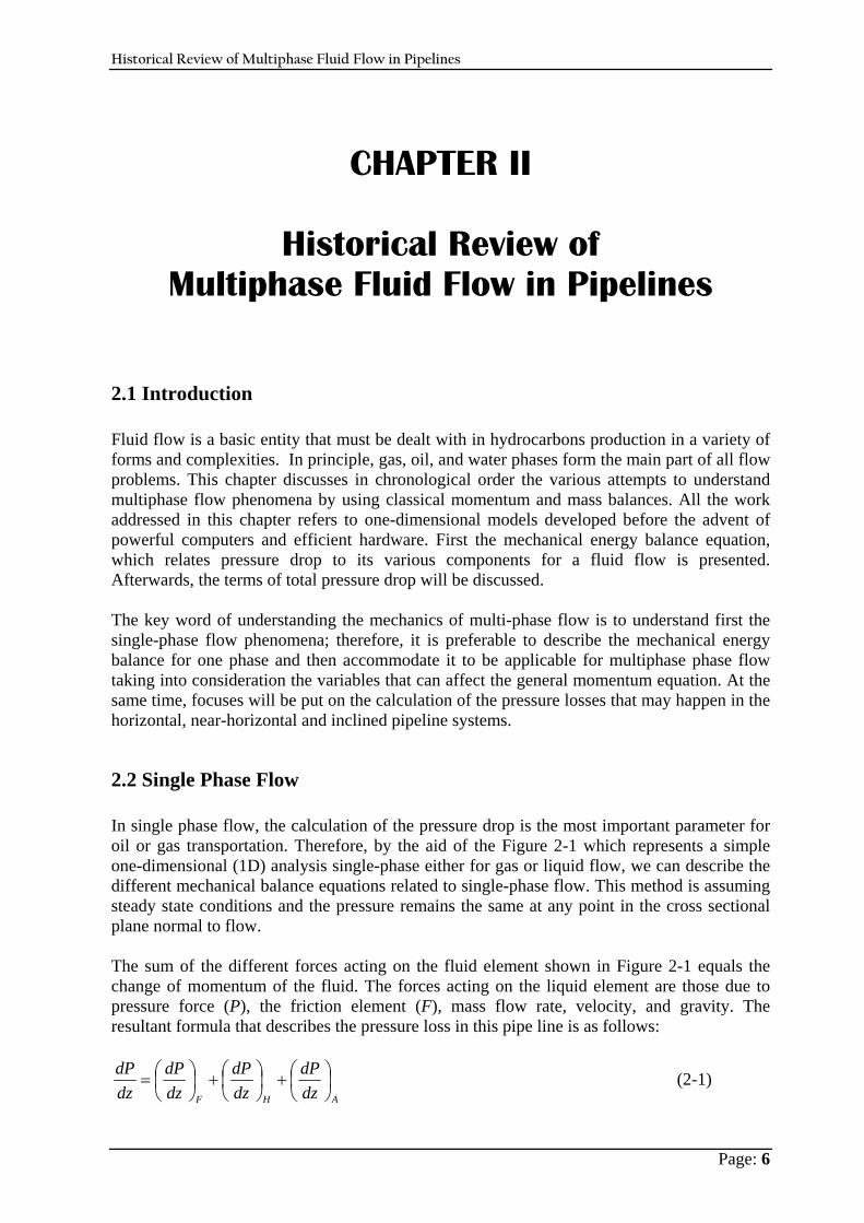
2.2 Single Phase Flow In single phase flow, the calculation of the pressure drop is the most important parameter for oil or gas transportation. Therefore, by the aid of the Figure 2-1 which represents a simple one-dimensional (1D) analysis single-phase either for gas or liquid flow, we can describe the different mechanical balance equations related to single-phase flow. This method is assuming steady state conditions and the pressure remains the same at any point in the cross sectional plane normal to flow. The sum of the different forces acting on the fluid element shown in Figure 2-1 equals the change of momentum of the fluid. The forces acting on the liquid element are those due to pressure force (P), the friction element (F), mass flow rate, velocity, and gravity. The resultant formula that describes the pressure loss in this pipe line is as follows:

AHF dzdP

dzdP

dzdP

dzdP

⎟⎠⎞

⎜⎝⎛+⎟

⎠⎞

⎜⎝⎛+⎟

⎠⎞

⎜⎝⎛= (2-1)

Historical Review of Multiphase Fluid Flow in Pipelines

Page: 7

Where:

dgfv

dzdP

cF 2

2ρ−=⎟

⎠⎞

⎜⎝⎛ ; (2-1a)

θρ singdzdP

H

=⎟⎠⎞

⎜⎝⎛ ; and (2-1b)

dzdvv

dzdP

A

ρ=⎟⎠⎞

⎜⎝⎛ (2-1c)

Figure 2-1: Schematic of a simple 1D single phase flow.

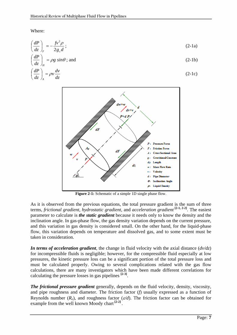
As it is observed from the previous equations, the total pressure gradient is the sum of three terms, frictional gradient, hydrostatic gradient, and acceleration gradient [ 2-1, 2-2]. The easiest parameter to calculate is the static gradient because it needs only to know the density and the inclination angle. In gas-phase flow, the gas density variation depends on the current pressure, and this variation in gas density is considered small. On the other hand, for the liquid-phase flow, this variation depends on temperature and dissolved gas, and to some extent must be taken in consideration. In terms of acceleration gradient, the change in fluid velocity with the axial distance (dv/dz) for incompressible fluids is negligible; however, for the compressible fluid especially at low pressures, the kinetic pressure loss can be a significant portion of the total pressure loss and must be calculated properly. Owing to several complications related with the gas flow calculations, there are many investigators which have been made different correlations for calculating the pressure losses in gas pipelines [ 2-3]. The frictional pressure gradient generally, depends on the fluid velocity, density, viscosity, and pipe roughness and diameter. The friction factor (f) usually expressed as a function of Reynolds number (Re), and roughness factor (ε/d). The friction factor can be obtained for example from the well known Moody chart [ 2-2] .

Historical Review of Multiphase Fluid Flow in Pipelines

Page: 8

In non-isothermal systems (such as single-phase flow from reservoirs, and transportation of the fluid over the sea bed) the temperature of the fluid varies significantly with the time. Many of the fluid properties such as density and viscosity are influenced by these changes in temperature, i.e. the change of temperature add more complications to the situation of the calculations of pressure drop in single-phase flow. Therefore, the previous equation will give a non accurate estimation for the pressure drop, and hence there are many researchers[ 2-4, 2-5] who worked in this area to re-derive the proper energy balance in order to estimate an accurate pressure drop due change in temperature.

2.3 Multiphase Flow 2.3.1 Background of Multiphase Flow Calculations Because of the potential economic attractiveness of two-phase flow, much attention has been focused on it beginning in the 1940’s. Therefore, since that date there exist varieties of technical papers and reports. Each is the result of a specific laboratory test or collected data, pilot plant or full scale systems using a limited number of fluids, flow rates and pipe sizes. There, from move on, focus will be on multiphase transportation and production pipelines. Transportation flow pipelines can be horizontal, vertical or inclined. No pipeline is perfectly horizontal along its whole length. Thus, the word “horizontal” merely signifies that line length is large compared to elevation changes. By the same the word “vertical” means that the elevation change is large compared to horizontal deviations. The primary difference between these two is the effect of gravity and line configuration on the character of fluid flow. The analysis of multi-phase flow closely follows the well-established previous method for single-phase flow equation, derived for the single-phase flow, applied to multi-phase or two-phase systems with a suitable assignation for mean prosperities for the mixture;

dzdv

gv

g sing

dgvf

dzdP m

c

mmm

cc

mmm ρρθρ++=

2

2

(2-2)

Computing mixture density and friction factor for the fluid mixture becomes complicated for two-phase flow. Two different methods, generalized and flow-pattern based may be used to express frictional, accelerational and potential pressure gradient during multiphase flow. The easiest or simplest one of the two – the generalized approach – attempts to develop methods for computing pressure drop and liquid holdup that will be applicable to all types of flow geometry and patterns. Within the generalized approach, two types of flow models can be used; homogeneous flow and separated flow model [ 2-2]. The homogeneous flow model assumes that the multiphase mixture behaves much like a homogeneous single – phase fluid, with property values that are some kind of average of the constituent phases. Once one decides which kind of averaging procedure to use, the computation procedure becomes typical to that of a single-phase system. Note that, the assumption of homogeneity pre-supposes a condition of no slip; that is that all phases move with the same in-situ velocity. Consequently, in-situ liquid fraction or liquid holdup is the same as the input fraction.

Historical Review of Multiphase Fluid Flow in Pipelines

Page: 9

In the other hand, the separated flow model recognizes that the phases are segregated or separated and that they move with non-equal velocities. Hence, the slip between the phases requires to be known in addition to the frictional interaction of the phases with the wall and among themselves. In the simple versions of the separated flow model, the frictional interactions among the phases are ignored. Consequently, even for the simplest model in this category, empirical correlations for computing liquid holdup and wall shear are needed, unlike the homogeneous model, where only wall shear is required. In the flow-pattern-based approach, an attempt is made to develop a mathematical model consistent with the observed physical phenomena for each flow regime. Through the modelling, only the most affecting factors are monitored, and unimportant effects, which do not add significantly to the solution accuracy, are ignored. Since flow patterns are somewhat different for horizontal, vertical, and inclined flows, pipe orientations are usually treated separately. Various flow patterns appear because of different hydrodynamic conditions. Therefore, this approach yields accurate working correlations, which are much more suitable for extrapolation and interpolation than the generalized approach. However, this method requires recognizing all relevant flow patterns by forehand. In most oil industry applications, the flow-pattern visualization is either impossible or uncertain; therefore, the pattern must be inferred based upon measured data, thereby introducing a possible source of error. A number of empirical or semi-theoretical correlations or maps are available for flow pattern delineation. Much progress has been made recently to model flow-pattern transition [ 2-2]. In another wider classification, the approaches applied to analyze multiphase flow can be classified into three categories, namely, empirical correlations, mechanistic models and numerical models. Empirical correlations create simplified relations among pertinent parameters which must be proved by some experimental data. The empirical correlations do not provide too much detail behind the behaviour of multiphase flow as a black box. They can sometimes yield excellent results but they are limited to the same conditions as the experiments [ 2-6]. Mechanistic models approximate the physical phenomenon by taking into consideration the most important processes and neglecting the less important effects that can complicate the problem but do not add more accuracy to the problem[ 2-7]. Finally, Numerical models introduce multi-dimensional Navier-Stokes equations for multiphase flow, therefore, more detailed information can be obtained from numerical models such as multi-dimensional distribution of the phases, dynamic flow regime transition and turbulent effects. They will be discussed in chapter IV. 2.3.2 Empirical Methods for Multiphase Flow Conventionally, most of the investigators analyze flow behaviour for the idealistic case of a truly horizontal line. Corrections are then made for inclined flow either uphill or downhill system. In a given length of line, several flow regimes occur because of different forces, elevations, and gas-liquid ratios. The following changes as liquid condenses from gas or gas is liberated from liquid, as dictated by physical properties and phase behaviour. Consideration of variables like all of the previous is a necessary part of developing a correlation. In general, the fluid flow in a horizontal system depends on several factors such as:

1. Flow rates of the gas and liquid. 2. Gas-liquid ratio. 3. Physical properties of the gas and liquid.

Historical Review of Multiphase Fluid Flow in Pipelines

Page: 10

4. Pipeline diameter. 5. The interfacial energies and shear forces involved in the interface between the phases.

One of the most famous empirical separated flow models is the Lockhart and Martinelli [ 2-8] (1949) approach. The Lockhart-Martinelli correlation was specifically derived for horizontal flow without significant acceleration. They proposed four combinations of viscous and turbulent flow assuming that the pressure drop for both gas and liquid were the same and the total pipe volume must be equal to the sum of the volumes occupied by the gas and liquid. The drawback of this method is that the data were obtained on 25 mm pipe or less. This raises the obvious question about application in much larger pipes. Since build-up of liquid in low spots and subsequent inclined flow is ignored, the effect of line diameter could be significant. In a small line, the capacity for build-up is limited. As diameter increases, it can be significant. Also, they assumed the liquid holdup is constant throughout the line. By implication, then the correlation does not include flow regimes. Therefore, its application to other situations, where frictional gradient is comparatively small can lead to significant errors. One aspect of this approach is that it skirts the flow pattern issue. This simplification has the advantage of avoiding the flow pattern discontinuities at the transition boundaries, although at the expense of model performance. Another well-known deficiency of this model is its unsatisfactory representation of the effect of system variables, in particular, flow rate. In addition, plug flow and severe slug flow would not fit the correlation. Also, bubble and mist flow do not fit the assumptions because there is a non-continuous phase interspersed throughout a continuous phase. Therefore, this calculation is designed for absolutely horizontal lines, containing two continuous phases, where the fraction of pipe area occupied by each phase essentially is constant throughout the line length. So this correlation can give a reasonable result only when these assumptions are met, regardless of the line diameter. Bertuzzi & Poettmann[ 2-9] (1956) presented an approach to determine the pressure drop due to flowing a two-phase (oil and gas) flow, using two-phase (f) friction factor related to gas-flow mass ratio, and two different Reynolds numbers, one for the gas phase, and the second for the liquid phase. They developed a new approach and translated it into graphical form to facilitate the computations and compared the results with 267 selected field data from 1000 data points with a good agreement, but it is considered a homogeneous phase flow which ignored the flow patterns of two phase flow and the slippage of gas over the liquid surface. To some extent, a good extension for Lockhart and Martinelli[ 2-8] correlation presented by Baker [ 2-10] (1958). Baker correlation introduced different flow regimes and introduced a correction for inclined flow through a small pipe diameter flow (1- to 4-in). For each of his regimes a series of equations was proposed to identify. Baker published a flow map for these regimes using two dimensionless groups. At that time, the Baker model is considered the modified and the more accurate extension of Lockhart and Martinelli approach. In parallel to Baker, Flanigan[ 2-11] (1958) published correlation similar to the Baker, except that he used the Panhandle-A equation as a reference and calculated the efficiency term differently to reduce the spread of data shown by Baker. His correlation is based on field tests of pipelines as large as 16-in diameter, and gives a realistic results very low gas velocity but it losses its applicability at higher gas rates. One of the most valuable study at that time, is the work of Duns and Ros[ 2-12] (1963), which has been applied for horizontal mist flow and vertical flow. They developed an empirical correlation for a large set of laboratory data. Their correlation considered a flow pattern-based

Historical Review of Multiphase Fluid Flow in Pipelines

Page: 11

model since they described four different flow regimes and assigned individual correlation for each regime. Their regimes are not like the current known flow regimes. A statistical study was made by a group directed by Dukler[ 2-13] (1964) in which about 20,000 data experimental points from pipe diameter 6 in or less were collected, then reduced to 2,600 data points by examining the data for internal consistency and apparent defects. They analyzed the data using about five different previous correlations. Lockhart and Martinelli was the best of the methods tested, but even this approach showed mean deviations of -6.6 to +38.3%. As expected, the Baker correlation gave better results on larger pipe lines with higher viscosity liquid up to 20 cp. Using three different correlations they tested liquid holdup and the results were random. Then they provided two different correlations, one in case of no slip effect and homogeneity, and the second assumes slip effect and that the ratio of each phase velocity to the average velocity is constant. Therefore, in general, Dukler’s data covered many pipe sizes and flow conditions, so his correlation results usable values. At low liquid and high gas rates, pressure drops tend to be less than the measured one. At high liquid rates coupled with high gas rates, pressure drops tend to be too high. Several investigators[ 2-14, 2-15, 2-16] under Brown’s direction developed a new correlation. This correlation based on test data which were taken on a field test unit consisting of two 1700 ft with diameters of 2- to 4-in. Using a computer, the calculation is an iterative solution for an incremental length of line of distance (ΔL) from the inlet between the pressures of that increment. Abdul-Majeed & Abu-Soof[ 2-17] (1967) modified Hagedorn-Brown correlation for calculating liquid holdup in which the original correlation gave under-predicted pressure loss by 20%, and they attributed this reduction to an under-prediction of liquid holdup. Because Dukler’s data covered many pipe sizes and flow conditions, Dukler et al.[ 2-18] correlation considered a good step in the trend of two-phase flow calculations. By 1966, Knowles[ 2-19] developed new flow regime maps using two dimensionless groups, modified Reynolds and Weber numbers. Beggs and Brill[ 2-20] (1973), modified and extended the present correlations for both horizontal and vertical flow considering angles of inclination from 0° to 90°. They utilized air-water as the fluids in 1 in and 1.5 in acrylic pipes. One of the large mistakes in this method and others is the use of higher order polynomial equations to fit the data. But it gives a good hint about increasing the liquid load in the low liquid load pipelines after a dramatic change in the temperature profile. By the mid 1970's, the possible combination of mathematical experiences that could be engaged in for two-phase flow had pretty well been exhausted. All of the variables that could be measured directly or indirectly has been identified and there were only so many ways that one could "mix and match" them or calculate them. The problem was to analyze and modify it, find its application limits. In 1977, Mandhane et al.[ 2-21] presented a brief comparisons for 16 of the previous correlations starting from Lockhart and Martinelli[ 2-8] (1949) to Beggs and Brill[ 2-20] correlation (1973) and proposed two-step prediction method for predicting friction pressure losses in horizontal gas-liquid flow pipes for slug flow and for dispersed bubble flow and suggested to use a computer program to solve it easily. In 1975 Brookbank and Fagiano[ 2-22] presented a review and comparisons of the available theory and practices of two phase flow and then proposed some modifications. For low liquid load multiphase flow, Hope and Nelson [ 2-23] (1977) reported data on a long North Sea

Historical Review of Multiphase Fluid Flow in Pipelines

Page: 12

pipeline containing about 5 bbl/MMscf of 56 API gravity condensate. These data support the hypothesis that one cannot develop fully turbulent flow in a wet gas line so long as liquid segregation is present; only partial turbulent flow is possible. Fully turbulent flow is possible only when the conditions are such that the liquid is dispersed in the gas phase. This, in turn, has implications for all methods which use a smooth pipe law for the frictional component calculation. This means that Dukler, Eaton, Beggs & Brill, approaches possess a potentially serious defect when applied to gas pipelines containing some liquid which operate normally under fully turbulent conditions [ 2-1]. A study of two-phase pipelines serving Prudhoe Bay field, Alaska has been reported by Brill et al.[ 2-24] (1980), 20 tests were conducted on two large pipe lines (12- and 16-in) under conditions where slug or froth flow were the primary flow regimes. The pipelines were divided into several segments for calculation purposes, a new segment being used whenever a finite change in inclination occurred. Pressure loss calculations were made by two methods, namely Dukler[ 2-13] and Beggs and Brill[ 2-20] approaches. But they modified to incorporate the holdup correlation of Eaton et al.[ 2-16] and the Beggs and Brill[ 2-20] approach was modified to include a rough pipe friction factor instead of the smooth pipe factor. Their findings showed that, liquid slug lengths were random. The mean length was around 650 ft and maximum length observed was 1600 ft. These data cannot be extrapolated to other systems but they showed that terminal equipment to handle such slugs must be larger than the average slug length. Mukherjee & Brill [ 2-25] (1983) studied the effect of inclination of two phase flow pipelines on the holdup correlations and presented a new empirical approach. They claimed that, their model is cable to determine of liquid holdup regardless of the angle of inclination and the direction of the flow. Since the prediction of pressure drop is a major objective in two-phase flow pipeline design. Goyon et al.[ 2-26] (1988) used a new procedure to calculate the pressure drop and temperature profile for two-phase flow in pipelines based on direct flash calculations at each pressure and temperature of interest. Flowing temperature distribution is predicted with different methods for pipelines. The Coulter and Bardon equation[ 2-27] commonly was used for pipeline temperature prediction. Although this equation originally was derived for gas flow, it was also used for single and two-phase flow. This equation is limited, however, by the assumptions of steady state heat transfer with a constant temperature environment and horizontal flow. Therefore, Alves et al.[ 2-28] (1992) tried to present a unified and general equation for flowing temperature prediction for pipelines, production or injection wells, under single or two-phase flow, over a wide range of inclination from horizontal to vertical. Experimental studies have been performed by Kang-Jepson[ 2-29] (2002) in a pipe diameter 10.16 cm and 36 m long. They investigated the flow regimes maps in ±2°. ±5°, and ±30° inclinations, using superficial oil velocities between 0.2 and 2 m/s, and gas between 1 and 14 m/s with a constant temperature and pressure 25° C and 0.13 MPa respectively. They concluded that the dominant regime was slug flow for upward inclinations, and as the liquid velocity increases, the gas velocity required for transition from plug to slug increases as well. Oddie et al.[ 2-30] (2003) studied experimentally the behaviour of the two and three phase flows in large inclined pipe. Their model was 11 m long, 15 cm diameter, using water-gas, oil-water, and oil-water-gas multiphase flows. The pipe inclination was varied from 0 to 92 degree, and flow rates of each phase were varied over wide ranges (water-gas flow, Qg varied

Historical Review of Multiphase Fluid Flow in Pipelines

Page: 13

from 5-100 m3/h, and for oil-water flow and oil-water-gas flow, Qo varies from 2-40 m3/h). Their fluids were Kerosene as an oil, tap water, and nitrogen. Nuclear densitometers as well as ten electrical probes at different locations along the pipe were used for accurate monitoring the steady-state and transient flow. They conducted 444 tests. Bubble, churn, elongated-bubble, slug and stratified flows were observed for water-gas and oil-water-gas flow, while dispersed flows were observed for oil-water flows. In a very good experimental work to study the multiphase transportation of gas loaded with a very low load of liquid in pipelines, Asante[ 2-31] studied the effect of increasing the liquid phase by small amount and showed that the pressure drop increases substantially with this small increasing of the liquid phase, sometimes double of dry gas value. The difference between the previous correlations depends to a large extent on how these variables are treated. They are valid only on the tested experimental conditions and variables. Therefore, it lacks the generality, and so the need for a general approach was quite urgent. In the next subsection, we will present the most important mechanistic models. 2.3.3 Mechanistic Models for Multiphase Flow

2.3.3.1 Physical Description of the Flow Patterns Flow regimes vary depending on operating conditions, fluid properties, flow rates and the orientation and geometry of the pipe through which the fluids flow. The determination of flow regimes in pipes on operation is not an easy task. Many investigators evaluate horizontal flow diagnosing the type of flow pattern existing or expected. As a result, the following discussion presents a general description of the multiphase fluid flow patterns in horizontal and near horizontal pipes. There are several methods that describe the flow patterns in a multiphase system made by many investigators[ 2-9, 2-10, 2-32]. Some on these classifications are to group all flow patterns three types, dispersed flow, separated flow and intermittent flow or a combination. Distributed flow regimes are characterized by a uniform phase distribution in both the radial and axial directions, such as bubble, mist, froth, where there is only one continuous phase, the other phase being distributed throughout this phase as drops or bubble. Segregated or separated flow regimes are characterized by a non-continuous phase in the radial direction and a continuous phase distribution in the axial direction, such as stratified, annular; both phases present are continuous with the gas phase moving faster with a resultant shear force at the interface. Intermittent flow regimes are characterized by being non-continuous in the axial and radial direction, and therefore exhibit locally unsteady behaviour, such as slug, plug, and elongated bubble flow, continuity of both phases is interrupted and a series on inertial and kinetic forces changes occur throughout the pipeline section. In horizontal and near horizontal pipes, Taitel and Dukler[ 2-32] (1976) proposed a model for general prediction of the flow regime transitions in two-phase gas-liquid flow for a smooth pipe and then, Taitel[ 2-33] extended this work to include the effect of roughness. He found that the effect of roughness can be neglected in all horizontal pipes for all transition boundaries

Historical Review of Multiphase Fluid Flow in Pipelines

Page: 14

except for the intermittent-dispersed bubble transition, but for inclined pipes the effect of roughness is shown to affect all transition boundaries. Therefore, they described six distinct flow regimes in horizontal two-phase flow, which in general agreement with the most of the other works in the area[ 2-34, 2-35, 2-2], as shown in Figure 2-2, as follows: 1. Stratified Smooth Flow [SSF]: At very low flow rates, the liquid phase flows through the

bottom part of the pipe, while the gas phase flows at the top. Consequently, the two phases are stratified and the interface between them is smooth.

2. Stratified Wavy Flow [SWF]: At somewhat higher gas flow rates than is needed for SSF,

the liquid and the gas phases are still separated, as before, but the interface becomes wavy. 3. Plug (or Elongated Bubble) Flow [PF]: If the gas flow rates are very low and the liquid

phase rates are higher than that is needed for SWF, the liquid could fill the entire pipe and flow as plugs. In that case, the gas flows as elongated bubbles near the top of the pipe owing to gravity.

4. Slug Flow [SF]: At higher gas flow rates the bubbles become large, filling up a

substantial portion of the flow cross section. The liquid slugs in between move violently downstream and are usually aerated by small bubbles. The distinction between plug and slug flow is difficult and becomes subjective because of similar appearances. Indeed, Taitel et al.[ 2-33] combined these two patterns into one and named them intermittent flow.

5. Annular Flow [AF]: At high gas rates, the gas flows through the center of the pipe and

the liquid flows along the tube wall, forming an annulus. This flow pattern is very similar to its counterpart in vertical flow, except that the liquid film is thicker at the bottom than at the top because of gravity in horizontal flow. It forms from stratified flow when the liquid flow rate is low and the gas flow rate is high enough to spread the liquid around the pipe wall.

6. Dispersed Bubbly Flow [DBF]: At low gas and very high liquid rates, the gas phase may

become dispersed as small bubbles in a continuous liquid phase. Similar to its counterpart in vertical flow, the shear energy of the turbulent liquid phase reduces the effect of gravity causing the gas bubbles to be disturbed more or less uniformly across the flow channel. The bubble concentration profile is still asymmetrical, with the peak occurring at some point above the pipe axis.

2.3.3.2 Flow Pattern Identifications and Transitions Models Figure 2-3 represents the typical flow pattern map of Petalas and Aziz[ 2-36], where Vsl and Vsg being the superficial liquid and gas velocity respectively. It shows how the flow regimes can differ by changing gas and liquid phase velocities. Therefore, at each couple of phase velocity different regime can exist. Nevertheless, there are some additional factors that are able to disturb this regime. From these factors, pipe inclination, fluid properties, the operating pressure. The step for flow pattern prediction begins with the assumption that a particular flow pattern exists and is followed by an examination of various criteria that establish the stability of the flow regime. If the flow regime is shown to be unstable, a new flow pattern is assumed and the procedure is repeated[ 2-36, 2-37] until found the proper regime. The selected regimes are stratified flow, intermittent flow, dispersed flow and annular flow. Moreover, a

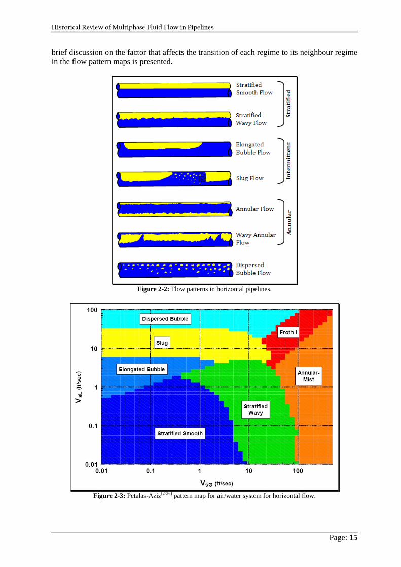
Historical Review of Multiphase Fluid Flow in Pipelines

Page: 15

brief discussion on the factor that affects the transition of each regime to its neighbour regime in the flow pattern maps is presented.

Figure 2-2: Flow patterns in horizontal pipelines.

Figure 2-3: Petalas-Aziz[ 2-36] pattern map for air/water system for horizontal flow.

Historical Review of Multiphase Fluid Flow in Pipelines

Page: 16

2.3.3.2.1 Stratified Flow Model Due to gravity, in stratified flow, liquid flows in the bottom portion of the pipe while the gas phase flows in the upper part of the pipe, as shown in Figure 2-4 Predicting the stability of the stratified flow regime needs the calculation of the liquid height, which can be obtained by writing the momentum balance equations, steady state, two fluids model approach and neglecting changes of phase velocity or liquid level as suggested by Taitel and Dukler [ 2-33]. Xiao et al.[ 2-38] and Gomez et al.[ 2-39]have adapted this approach and suggested an equation for estimating pressure gradient in both smooth and wavy stratified flows.

0sin =−−+⎟⎠⎞

⎜⎝⎛− θρττ gASS

dLdPA LLLwLiiL (2-3)

0sin =−−−⎟⎠⎞

⎜⎝⎛− θρττ gASS

dLdPA gGgwgiig (2-4)

Figure 2-4: Physical model for stratified flow in inclined pipelines. If the interfacial tension and liquid phase hydrostatic pressure gradient are neglected, the pressure gradients in both phases are the same. So, these two equations can be combined, and by eliminating the pressure gradient terms, yielding a combined momentum equation as follows:

( ) 0sin =−+⎟⎟⎠

⎞⎜⎜⎝

⎛⎟⎟⎠

⎞⎜⎜⎝

⎛++⎟

⎟⎠

⎞⎜⎜⎝

⎛− θρρ

ττττ g

AS

AS

AS

AS

GLg

i

L

i

wg

i

g

gwg

L

LwL (2-5)

This equation is an implicit formula for the dimensionless liquid height, Dhh LL /~

= , proposed by Taitel and Dukler[ 2-32] (1967). According to Xiao et al.[ 2-38] (1998) the liquid holdup can be calculated from a geometrical relationship as follow:

πϕϕ

2sin−

=LE , (2-6)

Where, ⎥⎦⎤

⎢⎣⎡ −= −

DhL21cos2 1ϕ , ϕ: subtended angle by interface (2-6a)

By calculating the liquid hold up (EL), one can calculate the pressure drop using one of the first two equations. The constitutive equations found in details in Xiao et al.[ 2-38].

Historical Review of Multiphase Fluid Flow in Pipelines

Page: 17

The Petalas and Aziz[ 2-36] model supposed that the profile of the gas liquid interface is flat. In fact the actual configuration makes a different contact area between the two fluids and between the fluids and pipe wall. Depending on the physical system involved, these variations can have prominent effects on the pressure drop and transport phenomena. Analytically, Brauner et al.[ 2-40] (1996) and Gorelik and Brauner[ 2-41] (1999) developed a new solution of the interface shape between two different immiscible fluids. The flow of oil-water mixtures in horizontal pipes experimentally and analytically has been investigated by Arirachakaran et al.[ 2-42] (1989) and they developed their own correlation for pressure gradient prediction for stratified and homogeneous flow patterns, and found that the frictional pressure drop is a function of mixture velocity, input water fraction, oil viscosity and temperature, and strongly depends on weather oil or water is the continuous phase . Vlachos et al.[ 2-43, 2-44] (1997 and 1999) improved the interfacial friction factor calculations by using an exponential expression of circumferential variation to calculate the average stress exerted by liquid on the pipe wall. Their model took into account flat profile transformation based on their previous study at 1997. Based on experimental data in two test facilities small and large-scale facilities, Fan et al. [ 2-45] (2005) proposed a relationship to predict liquid holdup and pressure gradient in stratified flow, as well as equations for wetted wall friction, liquid-wall friction, and interfacial friction factor, and they evaluated their result formulas with the results of OLGA 2000[ 2-46], which showed a little better performance than their model.

2.3.3.2.1.1 Transition between Smooth Stratified to Stratified Wavy Flow Taitel and Dukler[ 2-32] (1976a) introduced the idea of wave generation i.e. wavy stratified flow, which give quite different results for liquid hold up and pressure drop, and proposed that waves will form on the liquid surface once the gas velocity is increased beyond.

( )LGL

GLLG vs

gCosvρρ

θρρμ −≥

4 (2-7)

where, (s) is a sheltering coefficient, values ranging from 0.01 to 0.6 have been suggested from theories and experiments in the literatures, and so Taitel and Dukler used 0.01 value for (s) to match their experimental data, while Petalas and Aziz[ 2-36] (1998) and Xiao et al. [ 2-38] (1990) have taken the s-value as 0.06 based on a study by Andritsos[ 2-47]. This value is said to be more suitable especially for gas flow with liquids of high viscosity. For negative inclination, stratified flow in downwardly inclined pipes waves can develop under the influence of gravity even without presence of interfacial shear from the gas flow. The theory for the appearance of waves can be expressed in terms of a critical Froude number which varies from 0.5 to 2.2 depending on the roughness and whether the flow is laminar or turbulent. Barnea[ 2-48] (1982), recommended a limiting value of 1.5 for the critical Froude number. If the interfacial effects are considered in the calculation of the liquid height, this limit can predict smooth flow even at high liquid rates where the flow is known to be wavy. Petalas and Aziz [ 2-36] (1998) suggested that reducing the limit to 1.4 appears to resolve this problem.

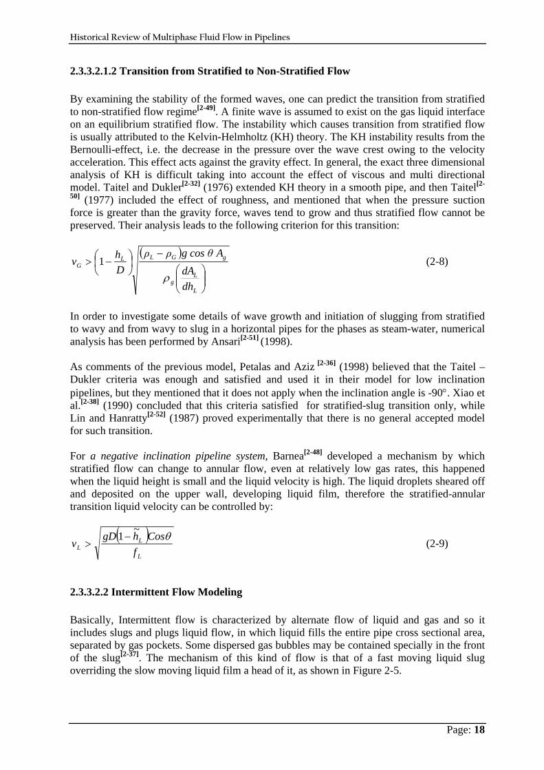
Historical Review of Multiphase Fluid Flow in Pipelines

Page: 18

2.3.3.2.1.2 Transition from Stratified to Non-Stratified Flow By examining the stability of the formed waves, one can predict the transition from stratified to non-stratified flow regime[ 2-49]. A finite wave is assumed to exist on the gas liquid interface on an equilibrium stratified flow. The instability which causes transition from stratified flow is usually attributed to the Kelvin-Helmholtz (KH) theory. The KH instability results from the Bernoulli-effect, i.e. the decrease in the pressure over the wave crest owing to the velocity acceleration. This effect acts against the gravity effect. In general, the exact three dimensional analysis of KH is difficult taking into account the effect of viscous and multi directional model. Taitel and Dukler[ 2-32] (1976) extended KH theory in a smooth pipe, and then Taitel[ 2-

50] (1977) included the effect of roughness, and mentioned that when the pressure suction force is greater than the gravity force, waves tend to grow and thus stratified flow cannot be preserved. Their analysis leads to the following criterion for this transition:

( )

⎟⎟⎠

⎞⎜⎜⎝

⎛

−⎟⎠⎞

⎜⎝⎛ −>

L

Lg

gGLLG

dhdA

A g cos θρρDhv

ρ1 (2-8)

In order to investigate some details of wave growth and initiation of slugging from stratified to wavy and from wavy to slug in a horizontal pipes for the phases as steam-water, numerical analysis has been performed by Ansari[ 2-51] (1998). As comments of the previous model, Petalas and Aziz [ 2-36] (1998) believed that the Taitel –Dukler criteria was enough and satisfied and used it in their model for low inclination pipelines, but they mentioned that it does not apply when the inclination angle is -90°. Xiao et al.[ 2-38] (1990) concluded that this criteria satisfied for stratified-slug transition only, while Lin and Hanratty[ 2-52] (1987) proved experimentally that there is no general accepted model for such transition. For a negative inclination pipeline system, Barnea[ 2-48] developed a mechanism by which stratified flow can change to annular flow, even at relatively low gas rates, this happened when the liquid height is small and the liquid velocity is high. The liquid droplets sheared off and deposited on the upper wall, developing liquid film, therefore the stratified-annular transition liquid velocity can be controlled by:

( )L

LL f

CoshgDv

θ~1−> (2-9)

2.3.3.2.2 Intermittent Flow Modeling Basically, Intermittent flow is characterized by alternate flow of liquid and gas and so it includes slugs and plugs liquid flow, in which liquid fills the entire pipe cross sectional area, separated by gas pockets. Some dispersed gas bubbles may be contained specially in the front of the slug[ 2-37]. The mechanism of this kind of flow is that of a fast moving liquid slug overriding the slow moving liquid film a head of it, as shown in Figure 2-5.

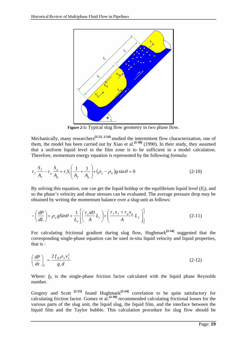
Historical Review of Multiphase Fluid Flow in Pipelines

Page: 19

Figure 2-5: Typical slug flow geometry in two phase flow.

Mechanically, many researchers[ 2-53, 2-54] studied the intermittent flow characterization, one of them, the model has been carried out by Xiao et al.[ 2-38] (1990). In their study, they assumed that a uniform liquid level in the film zone is to be sufficient in a model calculation. Therefore, momentum energy equation is represented by the following formula:

( ) 0sin11=−+⎟

⎟⎠

⎞⎜⎜⎝

⎛++− θρρτττ g

AAS

AS

AS

GLgf

iig

gg

f

ff (2-10)

By solving this equation, one can get the liquid holdup or the equilibrium liquid level (Ef), and so the phase’s velocity and shear stresses can be evaluated. The average pressure drop may be obtained by writing the momentum balance over a slug-unit as follows:

⎥⎥⎦

⎤

⎢⎢⎣

⎡⎟⎟⎠

⎞⎜⎜⎝

⎛ ++⎟

⎠⎞

⎜⎝⎛+=⎟

⎠⎞

⎜⎝⎛− f

ggffs

s

uu L

Ass

LA

DL

gSindLdP ττπτ

θρ 1 (2-11)

For calculating frictional gradient during slug flow, Hughmark[ 2-54] suggested that the corresponding single-phase equation can be used in-situ liquid velocity and liquid properties, that is :

dgvf

dzdP

c

LLfL

F

22 ρ=⎟

⎠⎞

⎜⎝⎛ (2-12)

Where: ffL is the single-phase friction factor calculated with the liquid phase Reynolds number. Gregory and Scott [ 2-55] found Hughmark[ 2-54] correlation to be quite satisfactory for calculating friction factor. Gomez et al.[ 2-39] recommended calculating frictional losses for the various parts of the slug unit, the liquid slug, the liquid film, and the interface between the liquid film and the Taylor bubble. This calculation procedure for slug flow should be

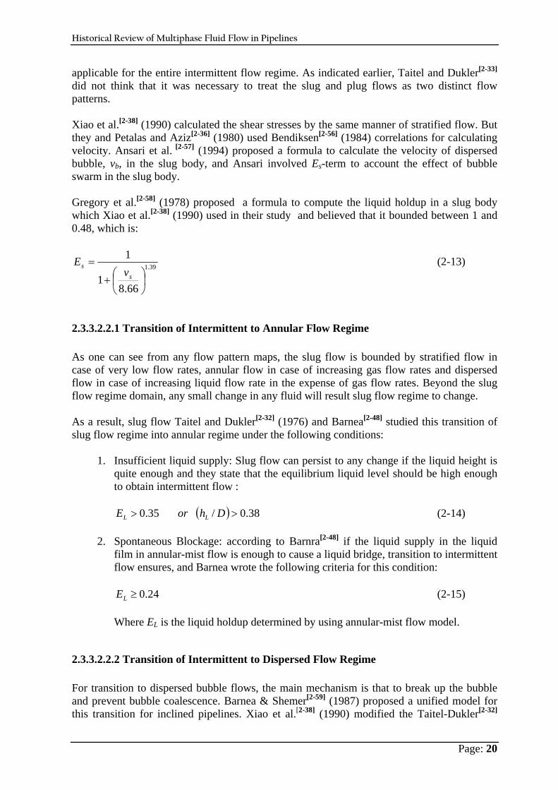
Historical Review of Multiphase Fluid Flow in Pipelines

Page: 20

applicable for the entire intermittent flow regime. As indicated earlier, Taitel and Dukler[ 2-33] did not think that it was necessary to treat the slug and plug flows as two distinct flow patterns. Xiao et al.[ 2-38] (1990) calculated the shear stresses by the same manner of stratified flow. But they and Petalas and Aziz[ 2-36] (1980) used Bendiksen[ 2-56] (1984) correlations for calculating velocity. Ansari et al. [ 2-57] (1994) proposed a formula to calculate the velocity of dispersed bubble, vb, in the slug body, and Ansari involved Es-term to account the effect of bubble swarm in the slug body. Gregory et al.[ 2-58] (1978) proposed a formula to compute the liquid holdup in a slug body which Xiao et al.[ 2-38] (1990) used in their study and believed that it bounded between 1 and 0.48, which is:

39.1

66.81

1

⎟⎠⎞

⎜⎝⎛+

=s

sv

E (2-13)

2.3.3.2.2.1 Transition of Intermittent to Annular Flow Regime As one can see from any flow pattern maps, the slug flow is bounded by stratified flow in case of very low flow rates, annular flow in case of increasing gas flow rates and dispersed flow in case of increasing liquid flow rate in the expense of gas flow rates. Beyond the slug flow regime domain, any small change in any fluid will result slug flow regime to change. As a result, slug flow Taitel and Dukler[ 2-32] (1976) and Barnea[ 2-48] studied this transition of slug flow regime into annular regime under the following conditions:

1. Insufficient liquid supply: Slug flow can persist to any change if the liquid height is quite enough and they state that the equilibrium liquid level should be high enough to obtain intermittent flow :

( ) 38.0/35.0 >> Dh or E LL (2-14)

2. Spontaneous Blockage: according to Barnra[ 2-48] if the liquid supply in the liquid film in annular-mist flow is enough to cause a liquid bridge, transition to intermittent flow ensures, and Barnea wrote the following criteria for this condition:

EL 24.0≥ (2-15) Where EL is the liquid holdup determined by using annular-mist flow model.

2.3.3.2.2.2 Transition of Intermittent to Dispersed Flow Regime For transition to dispersed bubble flows, the main mechanism is that to break up the bubble and prevent bubble coalescence. Barnea & Shemer[ 2-59] (1987) proposed a unified model for this transition for inclined pipelines. Xiao et al.[ 2-38] (1990) modified the Taitel-Dukler[ 2-32]

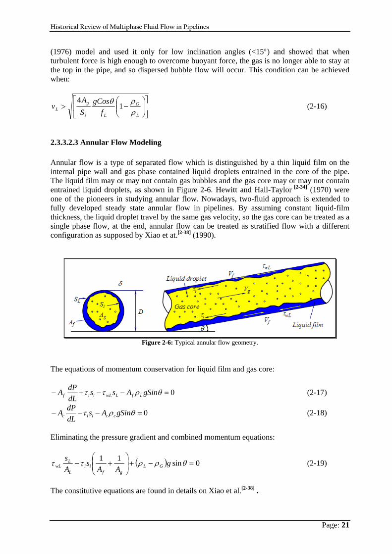
Historical Review of Multiphase Fluid Flow in Pipelines

Page: 21

(1976) model and used it only for low inclination angles (<15°) and showed that when turbulent force is high enough to overcome buoyant force, the gas is no longer able to stay at the top in the pipe, and so dispersed bubble flow will occur. This condition can be achieved when:

⎥⎦

⎤⎢⎣

⎡⎟⎟⎠

⎞⎜⎜⎝

⎛−>

L

G

Li

gL f

gCosSA

vρρθ 1

4 (2-16)

2.3.3.2.3 Annular Flow Modeling Annular flow is a type of separated flow which is distinguished by a thin liquid film on the internal pipe wall and gas phase contained liquid droplets entrained in the core of the pipe. The liquid film may or may not contain gas bubbles and the gas core may or may not contain entrained liquid droplets, as shown in Figure 2-6. Hewitt and Hall-Taylor [ 2-34] (1970) were one of the pioneers in studying annular flow. Nowadays, two-fluid approach is extended to fully developed steady state annular flow in pipelines. By assuming constant liquid-film thickness, the liquid droplet travel by the same gas velocity, so the gas core can be treated as a single phase flow, at the end, annular flow can be treated as stratified flow with a different configuration as supposed by Xiao et at.[ 2-38] (1990).

Figure 2-6: Typical annular flow geometry.

The equations of momentum conservation for liquid film and gas core:

0=−−+− θρττ gSinAssdLdPA LfLwLiif (2-17)

0=−−− θρτ gSinAsdLdPA cciic (2-18)

Eliminating the pressure gradient and combined momentum equations:

( ) 0sin11=−+⎟

⎟⎠

⎞⎜⎜⎝

⎛+− θρρττ g

AAs

As

GLgf

iiL

LwL (2-19)

The constitutive equations are found in details on Xiao et al.[ 2-38] .

Historical Review of Multiphase Fluid Flow in Pipelines

Page: 22

2.3.3.2.3.1 Annular Flow Transition to Intermittent Flow Barnea[ 2-48] and Petalas and Aziz [ 2-36] (1998) suggested two mechanisms to help annular flow to resist modification. Although they are revised to account for the difference in the modelling assumptions, the transition proposed by Barnea is divided into two mechanisms, the first mechanism based on the observation that the minimum interfacial shear stress is associated with a change in the direction of the velocity profile in the film. If the velocity profile becomes negative, stable annular flow can not be maintained and the transition to intermittent flow occurs which is relevant during uphill flow. The second mechanism occurs when the supply of liquid in the film is sufficient to cause blockage of the gas core by bridging the pipe. This can be happen if the liquid exceeds one half of the value associated with maximum packing density of uniformly sized gas bubble.

2.3.3.2.4 Dispersed Flow Modeling In this flow regime, gas phase dispersed and distributed throughout the liquid phase which fills the whole pipeline system. These gas bubbles may or may not have the same size, and may and may not distribute regularly as shown in Figure 2-7, and so the bubble size varies depending on the boundary conditions and fluid properties. This kind of flow appears at very high liquid flow rate when the turbulent is very strong. In such cases a homogeneous model may be applied. Depending on gas and liquid rates, there may or may not be slip between the phases. In simplest case, Xiao et al.[ 2-38] (1990) assumed no slippage between the phases, and so the pseudo-single phase model with the average properties is suitable for modelling dispersed flow, and the liquid holdup can be calculated as:

t

sLL V

vE = , (2-20)

The transitional bubble velocity (Vt) is calculated from [ bmot vvCv += ], the distribution parameter Co ranges from 1 to1.5 in which higher values being related to high bubble concentrations and high velocities at the center line in case of laminar flow. In case of turbulent flow Co approaches 1. Petalas and Aziz [ 2-36] (1998) and Kaya et al.[ 2-60] (1999) used Co 1.2 while Gomez et al.[ 2-61] (1999) used 1.15 in their model.

Figure 2-7: Schematic diagram of dispersed flow regime.

The pressure gradient also can be calculated as in single phase flow with average mixture density and velocity as follow:

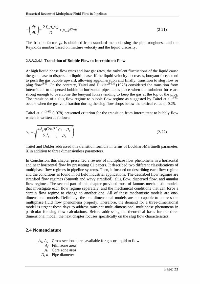
Historical Review of Multiphase Fluid Flow in Pipelines

Page: 23

θρρ

gSinD

vfdLdP

mmmm +=⎟

⎠⎞

⎜⎝⎛−

22 (2-21)

The friction factor, fm is obtained from standard method using the pipe roughness and the Reynolds number based on mixture velocity and the liquid viscosity.

2.3.3.2.4.1 Transition of Bubble Flow to Intermittent Flow At high liquid phase flow rates and low gar rates, the turbulent fluctuations of the liquid cause the gas phase to disperse in liquid phase. If the liquid velocity decreases, buoyant forces tend to push the gas bubble upward, allowing agglomeration and finally, transition to slug flow or plug flow[ 2-2]. On the contrary, Taitel and Dukler[ 2-32] (1976) considered the transition from intermittent to dispersed bubble in horizontal pipes takes place when the turbulent force are strong enough to overcome the buoyant forces tending to keep the gas at the top of the pipe. The transition of a slug flow regime to bubble flow regime as suggested by Taitel et al.[ 2-62] occurs when the gas void fraction during the slug flow drops below the critical value of 0.25. Taitel et al.[ 2-33] (1978) presented criterion for the transition from intermittent to bubbly flow which is written as follows:

⎟⎟⎠

⎞⎜⎜⎝

⎛ −=

L

gL

Li

gL fS

gCosAv

ρρρθ4

(2-22)

Taitel and Dukler addressed this transition formula in terms of Lockhart-Martinelli parameter, X in addition to three dimensionless parameters. In Conclusion, this chapter presented a review of multiphase flow phenomena in a horizontal and near horizontal flow by presenting 62 papers. It described two different classifications of multiphase flow regimes in pipeline systems. Then, it focused on describing each flow regime and the conditions as found in oil field industrial applications. The described flow regimes are stratified flow regimes (Smooth and wavy stratified), slug flow, dispersed flow, and annular flow regimes. The second part of this chapter provided most of famous mechanistic models that investigate each flow regime separately, and the mechanical conditions that can force a certain flow regime to change to another one. All of these mechanistic models are one-dimensional models. Definitely, the one-dimensional models are not capable to address the multiphase fluid flow phenomena properly. Therefore, the demand for a three-dimensional model is urgent these days to address transient multi-dimensional multiphase phenomena in particular for slug flow calculations. Before addressing the theoretical basis for the three dimensional model, the next chapter focuses specifically on the slug flow characteristics.

2.4 Nomenclature

Ag, AL Cross-sectional area available for gas or liquid to flow Af Film zone area Ac Core zone area

D, d Pipe diameter

Historical Review of Multiphase Fluid Flow in Pipelines

Page: 24

dz, ΔL Pipe length EL Liquid hold up Es Liquid holdup in a slug body

f Friction factor F Friction force ffL Single phase friction factor

fm, fL Friction factor of mixture and liquid phase respectively g Acceleration owing to gravity

gc Gravitational conversion factor, 32.17 ft/sec2 hL Liquid height

Lu, Lf, Ls Slug unit, film zone, and slug body length respectively P Pressure force

Qg Gas flow rate Qo Oil flow rate Re Reynolds number

sg, sL Gas wetted and liquid wetted periphery v Fluid velocity

vG, vL Gas and liquid velocity respectively vm Mixture velocity vs Slug velocity

vsg Superficial gas velocity vsl Superficial liquid velocity Vt Transitional bubble velocity w Mass flow rate of fluid

Lh~ Dimensionless liquid height

ϕ Subtended angle by interface θ, Inclination angle

ρ, ρL, ρG, ρm Fluid density, liquid, gas and mixture density respectively ε/d Pipe roughness

dP/dz Pressure gradient (dP/dz)A Acceleration pressure gradient (dP/dz)F Frictional pressure gradient (dP/dz)H Static pressure gradient

τi, τwg, τwL, Interface, gas-wall, liquid-wall shear stress

2.5 References

2-1. Boyd, O. W.: Petroleum Fluid Flow Systems, Campbell Petroleum Series, Norman, Oklahoma, USA, August 1983.

2-2. Hasan, A. R. and Kabir, C. S.: Fluid Flow and Heat Transfer in Wellbores, Society of Petroleum Engineers (SPE), Richardson, Texas, USA, 2002.

2-3. Cullender, M. H. and Smith, R. V.: “Practical Solution of Gas Flow Equations for Wells and Pipelines with Large Temperature Gradients,” Transaction of AIME 207, 1956.

2-4. Dikken, B. J.: “Pressure Drop in Horizontal Wells and its Effect on Production Performance,” JPT, Pages 1426-1433, November 1990.

2-5. Ouyang, L. B., Arbabi, S. and Aziz, K.: “A Single-Phase Wellbore Flow Model for Horizontal, Vertical and Slanted Wells,” SPEJ, Pages 124-133, June 1998.

Historical Review of Multiphase Fluid Flow in Pipelines

Page: 25

2-6. Xiaodong Zhao, M. S.: Mechanistic-Based Models for Slug Flow in Vertical Pipes, Ph. D. Thesis, Texas Tech University, May 2005.

2-7. Taitel, Y.: “Advances in Two Phase Flow Mechanistic Modelling,” SPE Paper 27959, SPE Journal, May 15, 1995.

2-8. Lockhart, R. W. and Martinelli, R. C.: “Proposed Correlation of Data for Isothermal Two-Phase Two Component Flow in Pipes,” Chemical Engineering Progress, Vol. 45, Pages 39-48, 1949.

2-9. Bertuzzi, A. F., Tek, M. R. and Poettmann, F. H.: “Simultaneous Flow of Liquid and Gas through Horizontal Pipe,” Petroleum Transactions, AIME, 17-24, Vol. 207, 1956.

2-10. Baker, O.: “Multiphase Flow in Pipe Lines,” Oil and Gas Journal, Nov. 10, 156, 1958.

2-11. Flanigan, O.: “Effect of Uphill Flow on Pressure Drop in Design of Two-Phase Gathering Systems”, Oil and Gas Journal, Vol. 56, 1958.

2-12. Duns, H. and Ros, N. C. J.: “Vertical Flow of Gas and Liquid Mixtures in Wells,” Proc., 6th World Petroleum Congress, Tokyo 451, 1963.

2-13. Dukler, A. E., Wicks, M. and Cleveland, R. G.: “Frictional Pressure Drop in Two-Phase Flow: A Comparison of Existing Correlations for Pressure Loss and Hold-Up,” AIChE J., 38, 1964.

2-14. Eaton, B. A. and Brown, K. E.: “A Joint Industry-University Research Project- Technical Report-University of Texas”, JPT, Feb.-Oct. 1965.

2-15. Andrews, D. E. and Brown, K. E.: Technical Report, Austin, TX, University of Texas, October, 1965.

2-16. Eaton, B. A., Andrews, D. E. and Knowles, C. R., Silberberg, I. H., and Brown, K. E.: “The Prediction of Flow Patterns, Liquid Holdup and Pressure Losses Occurring During Continuous Two-Phase Flow in Horizontal Pipelines,” SPE Paper 1525 & Journal of Petroleum Technology, Vol. 19, June 1967.

2-17. Abdul-Majeed, G. H. and Abu-Soof, N. B.: “An Improved Revision to Hagedorn and Brown Liquid Holdup Correlation,” SPE Paper 17122 & SPE of Production Engineering, July 1967.

2-18. Dukler, A. E. et al.: “Frictional Pressure Drop in Two Phase Flow,” AIChE Journal, Vol. 10, Pages 38-43, Jan. 1964.

2-19. Knowles, C.R.: The Effects of Flow Patterns of Pressure Loss in Multiphase Horizontal Flow, M.S. Thesis, the University of Texas, Austin, 1965.

2-20. Beggs, H. D. and Brill, J. P.: “A Study of Two-Phase Flow in Inclined Pipes,” JPT, Vol. 25, No. 5, Pages 607-617, May 1973.

2-21. Mandhane, J. M., Gregory, G. A. and Aziz, K.: “Critical Evaluation of Friction Pressure Drop Prediction Method for Gas-Liquid Flow in Horizontal Pipes,” JPT, Pages 1348-1358, Oct. 1977.

2-22. Brookbank, M. R. and Fagiano, P. M. J.: “A Review of the Theory and Practice of Two-Phase Flow in Gas-Liquid Transmission Systems,” SPE Paper 5264, Presented at the SPE-European Spring Meeting 1975 of the SPE of AIME, held in London, England, April 14-15, 1975.

2-23. Hope, P. M. and Nelson, R. G.: “A New Approach to the Design of Wet-Gas Pipelines,” ASME Conference, Houston, Sept. 1977 and Oil and Gas Journal, P. 93, October 31, 1977.

2-24. Brill, J. P., Schmidt, Z., Coberly, W. A. Herring, J. D. and Moore, D. W.: “Analysis of Two-Phase Tests in Large-Diameter Flow Lines in Prudhoe Bay Field,” SPE Journal, Vol. 271, Pages 363-378, June 1981.

Historical Review of Multiphase Fluid Flow in Pipelines

Page: 26

2-25. Mukherjee, H. and Brill, J. P.: “Liquid Holdup Correlations for Inclined Two-Phase Flow,” SPE Paper 10923 & JPT, Vol. 35, Issue 5, Pages 1003-1008, May 1983.

2-26. Goyon, J. C., Shoham, O., and Brill, J. P. : “Analysis of Computational Procedures for Multicomponent Flow in Pipelines,” SPE Paper 17573, Presented at SPE International meeting on Petroleum Engineering, held in Tianjin, China, Nov. 1-4, 1988.

2-27. Coulter, D. M. and Bardon, M. F.: “Revised Equation Improves Flowing Gas Temperature Prediction,” Oil & Gas Journal, Vol. 26, Pages 107-108, Feb.1979.

2-28. Alves, I. N., Alhanatl, F. J. S. and Shoham, O.: “A Unified Model for Predicting Flowing Temperature Distribution in Wellbores and Pipelines,” SPE Paper 20632 & SPE Production Engineering, Vol. 7, No. 4, Pages 363-367, Nov. 1992.

2-29. Kang, C., Jepson, W. P. and Wang, H.: “Flow Regime Transitions in Large Diameter Inclined Multiphase Pipelines,” Paper No. 02243, Corrosion 2002.

2-30. Oddie, G., Shi, H., Durlofsky, L. J., Aziz, K., Pfeffer, B. and Holmes, J. A.: “Experimental Study of Two Phase and Three Phase Flows in Large Diameter Inclined Pipes,” International Journal of Multiphase Flow, Vol. 29, Issue 4, Pages 572-558, April 2003.

2-31. Asante, B.: Multiphase Transport of Gas and Low Loads of Liquids in Pipelines, Ph. D. dissertation, Chemical and Petroleum Engineering, University of Calgary, 2000. (http://hdl.handle.net/1880/40528).

2-32. Taitel Y. and Dukler A. E.: “A Model for Prediction Flow Regime Transitions in Horizontal and near Horizontal Gas-Liquid Flow,” AIChE J., Vol. 22, Pages 47-55, Jan. 1976.

2-33. Taitel, Y., Lee, N. and Dukler, A. E.: “Transition Gas-Liquid Flow in Horizontal Pipes-Modeling Flow Pattern Transitions,” AIChE J., Vol. 24, Issue 5, Pages 920-934, June 1978.

2-34. Hewitt, G. F. and Hall-Taylor, N. S.: Annular Two-Phase Flow, Pergamon Press, Oxford, UK. 1970.

2-35. Baker, O.: “Design of Pipe Simultaneous Flow of Oil and Gas,” Oil & Gas J., Vol. 26, Pages 185-190, July 1954.

2-36. Petalas N. and Aziz, K.: “A Mechanistic Model for Multiphase Flow in Pipes,” CIM 98-39, Proceedings, 49th Annual Technical Meeting of the Petroleum Society of the Canadian Institute of Mining (CIM), Calgary, Alberta, Canada, June 8-10, 1998.

2-37. Arirachakaran, S., Papadimitriou, D. A. and Jefferson, L.L. : “Intelligent Utilization of a Unitized Flow Pattern Prediction Model in Production System Optimization,” SPE Paper 22869, Presented at the 66th SPE Annual Technical Conference and Exhibition of SPE held in Dallas, Texas, Oct. 6-9, 1991.

2-38. Xiao, J. J., Shoham, O. and Brill, J. P.: “A Comprehensive Mechanistic Model for Two-Phase Flow in Pipelines,” Paper SPE 20631 Presented at the 1990 SPE Annual technical Conference and Exhibition, New Orleans, Louisiana, 23-26 Sept.

2-39. Gomez, L. E., Shoham, O., Schmidt, Z. Chokshi, R. N. and Tor Northug: “Unified Mechanistic Model for Steady-State Two-Phase Flow: Horizontal to Vertical Upward Flow,” SPE 65705 & SPEJ, Vol. 5, No. 3, Pages 339-350, Sept. 2000.

2-40. Brauner, N., Rovinsky, J. and Maron, D. M.: “Analytical Solution of Laminar-Laminar Two-Phase Stratified Flow in Circular Conduits.” Chemical Engineering Communications, Vol. 141, Issue 1, Pages 103-143, Nov. 1994.

2-41. Gorelik, D. and Brauner N.: “The Interface Configuration in Two-Phase Stratified Pipe Flows,” International Journal of Multiphase Flow, Vol. 25, No.6, Pages 977-1007, September 1999.

Historical Review of Multiphase Fluid Flow in Pipelines

Page: 27

2-42. Arirachakaran, S., Oglesby, K. D., Malinowsky, M. S., Shoham, O. and Brill, J. P. : “An Analysis of Oil/Water Flow Phenomena in Horizontal Pipes,” SPE Paper 18836, Presented at the SPE Production Operations Symposium held in Oklahoma City, Oklahoma, March 13-14, 1989.

2-43. Vlachos, N. A., Paras, S. V. and Karabelas, A. J.: “Prediction of Holdup, Axial Pressure Gradient and Wall Shear Stress in Wavy Stratified and Stratified/Atomization Gas/Liquid Flow,” International Journal of Multiphase Flow, Vol. 25, Issue 2, Pages 365-376, March 1999.

2-44. Vlachos, N. A., Paras, S. V. and Karabelas, A. J.: “Liquid-to-Wall Shear Stress Distribution in Stratified/Atomization Flow,” International Journal of Multiphase Flow, Vol. 23, Issue 5, Pages 845-863, 1997.

2-45. Fan Y., Wang, Q., Zhang, H., Sarica, C. and Danielson, T. J.: “A Model to Predict Liquid Holdup and Pressure Gradient of Near-Horizontal Wet-Gas Pipelines,” SPE Paper 95674, Presented at the 2005 SPE Annual Technical Conference and Exhibition held in Dallas, Texas, USA, 9-12 October 2005.

2-46. Bendiksen K. H., Maines, D., Moe, R. and Nuland, S.: “The Dynamic Two Fluid Model OLGA: Theory and Application,” SPE Production Engineering, Vol. 6, Issue 2, Pages 171-180, May, 1991.

2-47. Andritsos, N. and Hanratty, T. J.: “Influence of Interfacial Waves in Stratified Gas-Liquid Flows,” AIChE J., Vol. 33, Pages 444-454, 1987.

2-48. Barnea, D., Shoham, O. and Taitel, Y.: “Flow Pattern Transition for Downward Inclined Two Phase Flow: Horizontal to Vertical,” Chemical Eng. Science, Vol. 37, No. 5, Pages 735-740, 1982.

2-49. Govier, G. W. and Aziz, K.: The Flow of Complex Mixtures in Pipes, van Nostrand Reinhold Co., New York City, 1972.

2-50. Taitel, Y.: “Flow Pattern Transition in Rough Pipes,” International Journal of Multiphase Flow, Vol. 3, Issue 6, Pages 597-601, December 1977.

2-51. Ansari, M. R.: “Numerical Analysis for Slugging of Steam-Water Stratified Two-Phase Flow in Horizontal Duct,” Fluid Dynamic Research, Vol. 22, Pages 329-344, 1998.

2-52. Lin, P. Y. and Hanratty, T. J.: “Effect of Pipe Diameter on Flow Pattern for Air-Water Flow in Horizontal Pipes,” International Journal of Multiphase Flow, Vol. 13, Pages 549-563, 1987.

2-53. Taitel, Y. and Barnea, D.: Two-Phase Slug Flow: Advances in Heat Transfer, Hartnett J. P. and Irvine Jr. T. F. ed., Vol. 20, Pages 83-132, Academic Press, 1990.

2-54. Hughmark, G. A.: “Holdup and Heat Transfer in Horizontal Slug Gas-Liquid Flow,” Chemical Engineering Science, Vol. 20, Pages 1007-101, 1965.

2-55. Gregory, G. A. and Scott, D. S.: “Correlation of Liquid Slug Velocity and Frequency in Horizontal Co-current Gas-Liquid Slug Flow,” AIChE J., Vol. 15. No. 6, Pages 933-935, 1969.

2-56. Bendiksen, K. H.: “An Experimental Investigation of the Motion of Long Bubbles in Inclined Tubes,” International Journal of Multiphase Flow, Vol. 4, Issue 4, Pages 467-483, Aug. 1984.

2-57. Ansari, A. M., Sylvester, N. D. and Brill, J. P.: “A Comprehensive Mechanistic Model for Upward Two-Phase Flow in Wellbores,” SPEPF, Pages 143-152, May 1994.

2-58. Gregory, G. A., Nicholson, M. K. and Aziz, K.: “Correlation of the Liquid Volume Fraction in the Slug for Horizontal Gas-Liquid Slug Flow,” International Journal of Multiphase Flow, Vol. 4, No. 4, Pages 33-39, 1978.

Historical Review of Multiphase Fluid Flow in Pipelines

Page: 28

2-59. Barnea, D. and Shemer, L.: “Void Fraction Measurements in Vertical Slug Flow: Applications to Slug Characteristics and Transition,” International Journal of Multiphase Flow, Vol. 15, Pages 495-504, 1989.

2-60. Kaya, A. S., Sarica, C. and Brill, J. P.: “Comprehensive Mechanistic Modeling of Two-Phase Flow in Deviated Wells,” SPE 56522, Presented at the 1999 SPE Annual Technical Conference and Exhibition held in Houston, Texas, 3-6 October 1999.

2-61. Gomez, L. E., Shoham. O. Schmidt, Z., Chokshi, R. N., Brown A. and Northug T.: “A Unified Mechanistic Model for Steady-State Two-Phase Flow in Wellbores and Pipelines,” SPE Paper 56520, Presented at the 1999 SPE Annual Technical Conference and Exhibition held in Huston, Texas, USA, 3-6 October 1999.

2-62. Taitel, Y., Barnea, D. and Dukler, A. E.: “Modelling Flow Pattern Transitions for Steady Upward Gas-Liquid Flow in Vertical Tubes,” AIChE J., Vol. 26, No. 3, Pages 345-354, 1980.

Slug Flow Characteristics

Page: 29

CHAPTER III

Slug Flow Characteristics

3.1 Introduction The subject of multiphase flow phenomena in pipeline systems have been studied since more than six decades, nevertheless, the experimental and mechanistic models presented previously were not able to lead to a full understanding of the multiphase flow mechanisms specially slug flow. Therefore, and a s results of the advent of the numerical power and computers, the era of numerical simulation begins to deal with the multiphase phenomena in oil field industry. Specifically, slug flow modelling, a few trials have been presented to model some of slug flow characteristics, like slug frequency and slug length. However, they are considered to be not accurate enough for pipelines and downstream equipments designs. To achieve more understanding to slug flow phenomena in pipeline systems, this chapter presents a complete review about slug flow characteristics in terms of slug flow sources and mechanisms, problems, slugging types, and how to prevent and alleviate this problematic flow. In the second part of this chapter, a literature review of slug flow mechanisms studied previously and comparisons between them in tabulated form are presented. The studied characteristics are slug length, slug frequency, holdup, and slug velocity.

3.2 Slug Flow Mechanisms and Problems There are a lot of operating conditions in oil field industry that can develop liquid slugs flow in pipelines. These slugs are a headache for oil producers and designers. Some of these mechanisms are listed below:

1. Transient effects: slugs may be produced as a result of transient effects along the pipeline such as pressure or flow rate changes. e.g. if a pipeline operating in stratified flow is subjected to an increase in gas flow rate or total production rate, one or more slugs may be produced as the equilibrium level drops towards a new state condition.

2. Start up and blow-down operations: when a pipeline is shut down, the liquid will

drain to the low points in the line, and when the line is restarted, this liquid may exit the pipeline in the form of slugs. Slugs may also form during depressurization due to high gas velocities, and so transient simulations can be used to estimate both of these types of slugs.

3. Pigging operations: in which pigs are run through pipelines for liquid inventory

control, maintenance and data logging, or cleaning and de-waxing, such pigs should be designed to control their length and pressure drops.

Slug Flow Characteristics

Page: 30

4. Terrain induced: slugs caused by significant elevation changes along the pipeline such as geographical features or vertical risers. They are system specific and more difficult to model than the other types of slugging[ 3-1].

As mentioned in the previous chapter, slug flow is an intermittent flow, i.e. the flow may vary from about 100% liquid to near 100% gas flow. This behaviour creates serious design and operating problems for the pertinent equipments. Practically, there are a lot of problems that can be arising from slug flow in oil field. Some of these are;

1. Rupture due to sudden opening of valves (water hammering). 2. Fatigue caused by repeated pressure impact. 3. High pressure loss for hydrodynamic slugging. 4. Pigging. 5. High pressure and overflow in separation facilities. 6. Cease of production in case of low flow rates. 7. Overload on gas compressors.

3.3 Slugging Types 3.3.1 Hydrodynamic Slugging When gas and liquid slowly flow in a horizontal pipe, the flow pattern will be initially a stratified pattern. By increasing the flow rates, waves will be created on the gas-liquid interface and the liquid might touch the top of the pipe creating slugs separated by gas pockets. In some cases, the gas has the ability to disperse as a bubble in the liquid phases especially in the front of the liquid slugs. By changing the flow rates again, different flow patterns can be created, depending on the fluid density, the pipe inclination, the pipe geometry, and the operating pressure. So at moderate gas and liquid flow rates, the hydrodynamic or normal slug can be formed 3.3.2 Terrain-Induced Slugging A hilly terrain pipeline consists of horizontal, uphill, and downhill pipe sections as shown in Figure 3-1. The terrain slugging is typically created near a dip of a flow line, can in principle only occur if there is downward flow. So, terrain-induced slugging is characterised by liquid accumulation at low points. The upstream gas is compressed until it overcomes the hydraulic head of the liquid; thereby, creating a long liquid slug that is moved and pushed in front of the expanding gas upstream[ 3-2]. 3.3.3 Severe Slugging Multiphase flowing in risers and highly inclined hilly terrain pipelines is classified as severe slug flow. The slugging formed in the offshore risers is represent the worst case of sever slugging operations. The mechanism for slug flow in a riser is shown in Figure 3-2 . As one can see from Figure 3-2, sever slugging operation characterized by four different operations; slug formation, slug movement into the separator (slug production), blowout, and finally, liquid fallback. All of these operations performed sequentially, where the liquid blocks the gas

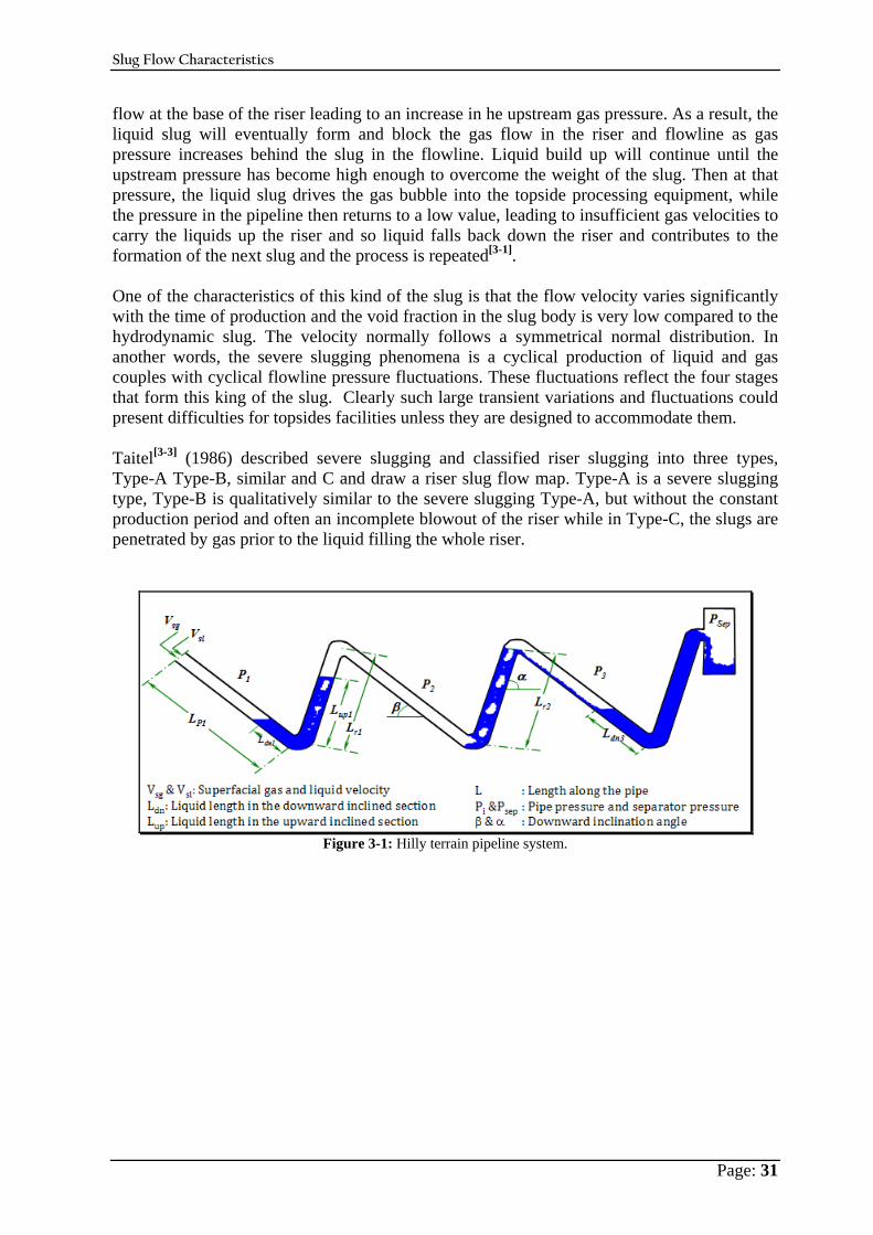
Slug Flow Characteristics

Page: 31

flow at the base of the riser leading to an increase in he upstream gas pressure. As a result, the liquid slug will eventually form and block the gas flow in the riser and flowline as gas pressure increases behind the slug in the flowline. Liquid build up will continue until the upstream pressure has become high enough to overcome the weight of the slug. Then at that pressure, the liquid slug drives the gas bubble into the topside processing equipment, while the pressure in the pipeline then returns to a low value, leading to insufficient gas velocities to carry the liquids up the riser and so liquid falls back down the riser and contributes to the formation of the next slug and the process is repeated[ 3-1]. One of the characteristics of this kind of the slug is that the flow velocity varies significantly with the time of production and the void fraction in the slug body is very low compared to the hydrodynamic slug. The velocity normally follows a symmetrical normal distribution. In another words, the severe slugging phenomena is a cyclical production of liquid and gas couples with cyclical flowline pressure fluctuations. These fluctuations reflect the four stages that form this king of the slug. Clearly such large transient variations and fluctuations could present difficulties for topsides facilities unless they are designed to accommodate them. Taitel[ 3-3] (1986) described severe slugging and classified riser slugging into three types, Type-A Type-B, similar and C and draw a riser slug flow map. Type-A is a severe slugging type, Type-B is qualitatively similar to the severe slugging Type-A, but without the constant production period and often an incomplete blowout of the riser while in Type-C, the slugs are penetrated by gas prior to the liquid filling the whole riser.

Figure 3-1: Hilly terrain pipeline system.

Slug Flow Characteristics

Page: 32

Figure 3-2: Severe slug formation and propagation procedures in a riser.

3.4 Slug Mitigation and Prevention Methods To ensure a stable production and transportation operations, methods for slug mitigation is quite required. Some of these approaches are: 1. Slug Catchers: they are some kind of separator with extra liquid capacity and special

design. It is very simple and robust but expensive due the vessel cost. There are several types and model designs for these catchers[ 3-1, 3-4, 3-5, 3-6, 3-7, 3-8, 3-9], such as finger type, multi-pipe type and vessel type.

2. Choking: in particular for riser flow, this method has shown to be effective for severe slug mitigation. It changes the slug flow to bubble flow regimes. It was invented first by Yocum[ 3-10] and Cady[ 3-11].

3. Gas injection: is based on injection of some gas at the bottom of the riser to increase the

velocity of the fluids, decreases liquid holdup and changes the flow regime to normal slugging or annular mist flow. It requires a gas source if the outlet gas is not enough. Gas injection plays on decreasing the slug length. One of its drawbacks is increasing compression cost.

4. Control schemes: they require a controller at the topside facilities to control the flow rates

in the risers and flowlines. In that sense they are similar to choking methods. Many researchers[ 3-9, 3-12, 3-13]have worked in this area and every one has his approach with different names such as:

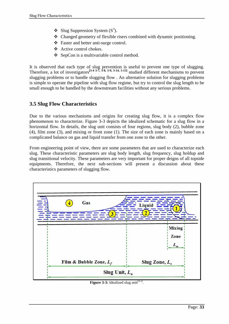
Slug Flow Characteristics

Page: 33

Slug Suppression System (S3). Changed geometry of flexible risers combined with dynamic positioning. Faster and better anti-surge control. Active control chokes. SepCon is a multivariable control method.

It is observed that each type of slug prevention is useful to prevent one type of slugging. Therefore, a lot of investigators[ 3-4 3-7, 3-8, 3-9, 3-14, 3-15] studied different mechanisms to prevent slugging problems or to handle slugging flow . An alternative solution for slugging problems is simple to operate the pipeline with slug flow regime, but try to control the slug length to be small enough to be handled by the downstream facilities without any serious problems.

3.5 Slug Flow Characteristics Due to the various mechanisms and origins for creating slug flow, it is a complex flow phenomenon to characterize. Figure 3-3 depicts the idealized schematic for a slug flow in a horizontal flow. In details, the slug unit consists of four regions, slug body (2), bubble zone (4), film zone (3), and mixing or front zone (1). The size of each zone is mainly based on a complicated balance on gas and liquid transfer from one zone to the other. From engineering point of view, there are some parameters that are used to characterize each slug. These characteristic parameters are slug body length, slug frequency, slug holdup and slug transitional velocity. These parameters are very important for proper deigns of all topside equipments. Therefore, the next sub-sections will present a discussion about these characteristics parameters of slugging flow.

Figure 3-3: Idealized slug unit[ 3-1].

Slug Flow Characteristics

Page: 34

3.5.1 Slug Length As shown in Figure 3-3, the slug length is the length of the liquid slug body for a slug unit. Accurate calculation of the slug length and slug length distribution is crucial for designing pipelines and separation facilities quantitatively. Earlier models deal with steady slug flow assuming constant length and shapes of liquid slugs and elongated bubbles as well as a constant elongated bubble propagation velocity. However, due to irregular character of slugging flow, a statistical means are required for its proper description [ 3-4]. Therefore, the practical design is to find the volume of the large slugs and design a separator or slug catcher able to handle this size of the slug, i.e. the design should based on an optimized value of slug length not only on the average length or smallest value. In order to predict and calculate the slug length, one should take in his mind some considerations and precautions to use and the correct slug length correlation for his design. The most important recommendations are mechanisms of the created slug. In another words, how the slugs created, as result of hydrodynamic effect, terrain effect, pigging, start-up and transient effect or riser effect. For hydrodynamic slugs, there is a rule says that the length of the slug is about 32 times the pipeline diameter if the flow line is completely horizontal. Indeed, if the flow line is not horizontal, terrain pipelines, this rule with not be valid for slug length estimation because the terrain will make the slugs grow or dissipate. For instance, several slugs can gather together in downward pipe section and form long slugs. There are a lot of slug length predictions which are based on laboratory work, which is limited to the experimental conditions and pipeline geometry, so they are not helpful in the field pipe line designing. A few correlation approaches have been developed based on field data. A list of the most famous published correlations for a horizontal pipeline is listed in Table 3-1 at the end of this sub-section. In 1981, Brill et al.[ 3-15] studied slug length characteristics (average length and length distribution) which mainly based on data collected from Prudhoe Bay Field for large pipeline diameters. This correlation predicts slug length of an order of magnitude longer than those suggested from earlier small diameter pipe lines based correlations. This correlation was based on a horizontal pipeline 12- tot 24-in diameter and 15000 ft long. This correlation compute slug length as a function of pipeline diameter only as follows:

( )[ ] 1.0ln4948.284144.25ln d Lsr +−= (3-1) Where, Lsr is the reference slug length at the end of the tested pipe in feet, and d stands for the pipeline diameter in inch. Because it was developed over a limited range of flow conditions it is suggested that use of the correlation be limited to the limited conditions. These condition are, pipeline diameter should be larger than 6-in, superficial gas velocity should be between 1.5 and 15 m/s and liquid superficial velocity should range from 0.3 and 1.5 m/s[ 3-1]. The Brill et al.[ 3-15] equation gives a slug length ranging between 300 to 350 times the pipe diameters., which is significantly higher than the range of 12-30 pipeline diameters from experimental data for small diameter pipeline[ 3-16]. It has become the industry standard design method, and has been used extensively by oil companies and contractors since 1979.

Slug Flow Characteristics

Page: 35

The prediction of slug characteristics for large-diameter pipes was studied with data collected from Prudhoe Bay field in Alaska flowlines by Scott et al.[ 3-17] (1989), in which the pipe line was fully instrumented with nuclear densitometers, turbine meters, flow meters, pressure, temperature sensors, and separator level indicators. Approximately, 19 million data points were collected on 12- 16- 20- and 24-in. diameter pipes. These data used statistically to address the slug characterises, such as slug length, bubble length, and hold-ups. They showed that the slug lengths do not remain constant and the slugs tend to grow as they flow through the pipeline. In 1994, Hill and Wood[ 3-18] presented a field study to investigate the nature of slug flow, slug length variation and distribution, and holdup variations for near-horizontal pipeline for British Petroleum Company (BP). It gives practical approach to compute slug length for this pipe line. Based on this approach, the slug length can be calculated by a mass balance. A simplistic approach to this calculation can be used, based on the conservative assumption that all liquid transport out of the system is the slug body, i.e. zero liquid velocity in the liquid film zone. This assumption leads to the following formula:

HF

ULssl

sls ,136002.1= (3-2)

Where:

Ls : the slug length in ft. Usl : the superficial liquid velocity, ft/sec. Hs : the liquid slug hold-up in the liquid slug. Fsl : the slug frequency, in Hz.

For a hilly terrain pipeline, most of the existing models are steady state models which are able to predict the average slug length for downstream capacity and pressure drop calculation models. By applying more than model, each one is giving different slug length value. Therefore, there are some conflicts in pressure drop calculations for pipeline design. Moreover; they are not capable to describe details about the flow characteristics like the maximum slug length expected at the exit of a hilly terrain pipeline, Al-Safran 2004 [ 3-19]. Presented a model to predict slug length distribution a long a hilly terrain pipelines. Al-Safran et al.[ 3-20] (2005) in their probabilistic/mechanistic modelling slug-length distribution study showed by statistical analysis that in addition to pipe diameter and mixture velocity, volumetric flow rate of the liquid film in the bubble region and the momentum exchange between the slug body and the liquid film correlate with the mean slug length. They[ 3-20] also suggested using the maximum slug length for proper separation or slug catcher design instead of the average slug length value On the other hand a probabilistic approach had been made by Bernlcot and Drouffe[ 3-21] (1991) to analyse the formation of slugs in inclined horizontal pipelines, and provided a new length distribution criteria which is verified against experimental data. It is observed from all the discussed slug length correlations, that each study gives a different approach and most of them are mainly based only in the pipeline diameter. This leads to the question, if the pipeline length has some effect or not?

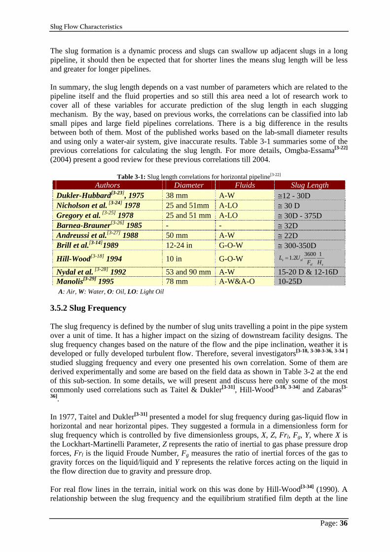
Slug Flow Characteristics

Page: 36

The slug formation is a dynamic process and slugs can swallow up adjacent slugs in a long pipeline, it should then be expected that for shorter lines the means slug length will be less and greater for longer pipelines. In summary, the slug length depends on a vast number of parameters which are related to the pipeline itself and the fluid properties and so still this area need a lot of research work to cover all of these variables for accurate prediction of the slug length in each slugging mechanism. By the way, based on previous works, the correlations can be classified into lab small pipes and large field pipelines correlations. There is a big difference in the results between both of them. Most of the published works based on the lab-small diameter results and using only a water-air system, give inaccurate results. Table 3-1 summaries some of the previous correlations for calculating the slug length. For more details, Omgba-Essama[ 3-22] (2004) present a good review for these previous correlations till 2004.

Table 3-1: Slug length correlations for horizontal pipeline[ 3-22] Authors Diameter Fluids Slug Length

Dukler-Hubbard[ 3-23], 1975 38 mm A-W ≅12 - 30D Nicholson et al. [ 3-24] 1978 25 and 51mm A-LO ≅ 30 D Gregory et al. [ 3-25] 1978 25 and 51 mm A-LO ≅ 30D - 375D Barnea-Brauner[ 3-26] 1985 - - ≅ 32D Andreussi et al.[ 3-27] 1988 50 mm A-W ≅ 22D Brill et al.[ 3-14]1989 12-24 in G-O-W ≅ 300-350D

Hill-Wood[ 3-18] 1994 10 in G-O-W ssl

sls HFUL 136002.1=

Nydal et al. [ 3-28] 1992 53 and 90 mm A-W 15-20 D & 12-16D Manolis[ 3-29] 1995 78 mm A-W&A-O 10-25D

A: Air, W: Water, O: Oil, LO: Light Oil 3.5.2 Slug Frequency The slug frequency is defined by the number of slug units travelling a point in the pipe system over a unit of time. It has a higher impact on the sizing of downstream facility designs. The slug frequency changes based on the nature of the flow and the pipe inclination, weather it is developed or fully developed turbulent flow. Therefore, several investigators[ 3-18, 3-30- 3-36, 3-34 ] studied slugging frequency and every one presented his own correlation. Some of them are derived experimentally and some are based on the field data as shown in Table 3-2 at the end of this sub-section. In some details, we will present and discuss here only some of the most commonly used correlations such as Taitel & Dukler[ 3-31], Hill-Wood[ 3-18, 3-34] and Zabaras[ 3-

36]. In 1977, Taitel and Dukler[ 3-31] presented a model for slug frequency during gas-liquid flow in horizontal and near horizontal pipes. They suggested a formula in a dimensionless form for slug frequency which is controlled by five dimensionless groups, X, Z, Frl, Fg, Y, where X is the Lockhart-Martinelli Parameter, Z represents the ratio of inertial to gas phase pressure drop forces, Frl is the liquid Froude Number, Fg measures the ratio of inertial forces of the gas to gravity forces on the liquid/liquid and Y represents the relative forces acting on the liquid in the flow direction due to gravity and pressure drop. For real flow lines in the terrain, initial work on this was done by Hill-Wood[ 3-34] (1990). A relationship between the slug frequency and the equilibrium stratified film depth at the line

Slug Flow Characteristics

Page: 37

start was denied. The equilibrium stratified film depth is calculated using the Taitel and Dukler [ 3-31] from the data given in and reproduced as a best fit equation was developed as:

leH

m

s

VDF ××= 68.210275.0 (3-3)

Where:

Fs : slug frequency (1/s) D : pipe diameter, ft Vm : mixture velocity, ft/s Hle : equilibrium stratified liquid holdup.

In 1994 , Hill-Wood[ 3-18]Then they extended their work to give us another formula according to the best fit average slug frequency equation valid for application to horizontal and near horizontal system, as follows:

[ ] [ ]lele HH

m

s eeV

DF '' 20524.091209.9 721.2400766.0729.24 ×÷ ×+×+−=⎥⎦

⎤⎢⎣

⎡ (3-4)

⎥⎦

⎤⎢⎣

⎡−×=

sllele

UHH 068.01' (3-5)

Zabaras [ 3-36] (1999) examined various correlations proposed in the literature for prediction of slug frequency in horizontal and inclined pipes. These correlations include both empirical correlations as well as mechanistic models. A total of eight published approaches were discussed and compared to slug flow frequency data but none was found satisfactory from his opinion. These correlations namely are Shell correlation[ 3-35], Tronconi[ 3-33] correlation (1990), Hill-Wood[ 3-34], Gregory-Scott[ 3-30] correlation, AGA[ 3-37] correlation, Greskovich-Shrier[ 3-38] correlation, Heywood–Richardson[ 3-32] correlation, and finally, Taitel-Dukler[ 3-31] correlation. For this reason, careful analysis indicated that slug frequency increases with inclination angle from horizontal line. With this in mind a correlation of the slug frequency data was attempted of the form:

( ) ( )θ25.02.12.1

sin75.2836.06.2120226.0 ×+⎥⎦

⎤⎢⎣

⎡+⎥

⎦

⎤⎢⎣

⎡= m

m

sls V

VgDVf (3-6)

Where;

Vsl : superficial gas velocity Vm : mixture velocity, θ : pipe line inclination angle (positive for upward inclined pipelines). G : gravity constant.

Therefore, Omgba-Essama[ 3-22] (2004) classified the previous models for calculating the slug frequency into two types. The first type is empirical models and the second one is phenomenological models. By correcting and updating Omgba-Essama[ 3-22], Table 3-2 gives a list of the most famous frequency correlations.

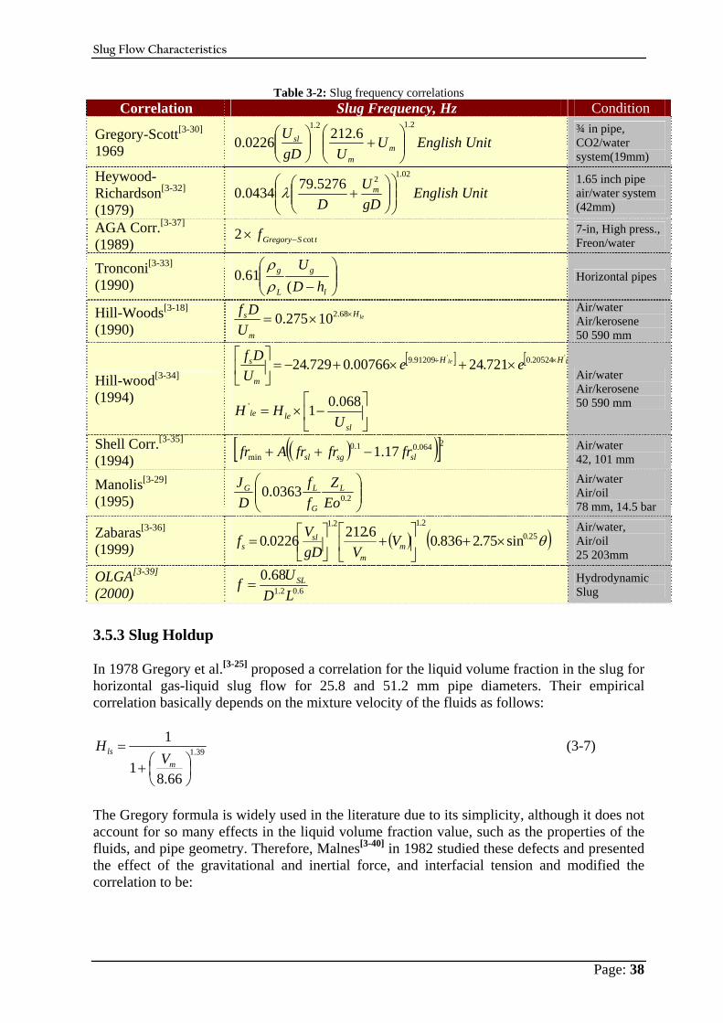
Slug Flow Characteristics

Page: 38

Table 3-2: Slug frequency correlations Correlation Slug Frequency, Hz Condition

Gregory-Scott[ 3-30] 1969

2.12.16.2120226.0 ⎟⎟

⎠

⎞⎜⎜⎝

⎛+⎟⎟

⎠

⎞⎜⎜⎝

⎛m

m

sl UUgD

U English Unit ¾ in pipe, CO2/water system(19mm)

Heywood-Richardson[ 3-32] (1979)

02.125276.790434.0 ⎟⎟⎠

⎞⎜⎜⎝

⎛⎟⎟⎠

⎞⎜⎜⎝

⎛+

gDU

Dmλ English Unit

1.65 inch pipe air/water system (42mm)

AGA Corr.[ 3-37] (1989) tSGregoryf cot2 −× 7-in, High press.,

Freon/water

Tronconi[ 3-33] (1990) ⎟⎟

⎠

⎞⎜⎜⎝

⎛− l

g

L

g

hDU

(61.0

ρρ

Horizontal pipes

Hill-Woods[ 3-18] (1990)

leH

m

s

UDf ××= 68.210275.0

Air/water Air/kerosene 50 590 mm

Hill-wood[ 3-34] (1994)

[ ] [ lele HH

m

s eeU

Df '' 20524.091209.9 721.2400766.0729.24 ×÷ ×+×+−=⎥⎦

⎤⎢⎣

⎡

⎥⎦

⎤⎢⎣

⎡−×=

sllele

UHH 068.01'

Air/water Air/kerosene 50 590 mm

Shell Corr.[ 3-35] (1994) ( )( )[ ]2064.01.0

min 17.1 slsgsl frfrfrAfr −++ Air/water 42, 101 mm

Manolis[ 3-29] (1995) ⎟⎟

⎠

⎞⎜⎜⎝

⎛2.00363.0

EoZ

ff

DJ L

G

LG Air/water Air/oil 78 mm, 14.5 bar

Zabaras[ 3-36] (1999) ( ) ( )θ25.0

2.12.1

sin75.2836.06.2120226.0 ×+⎥⎦

⎤⎢⎣

⎡+⎥

⎦

⎤⎢⎣

⎡= m

m

sls V

VgDVf

Air/water, Air/oil 25 203mm

OLGA[ 3-39]

(2000) 6.02.1

68.0LDUf SL= Hydrodynamic

Slug

3.5.3 Slug Holdup In 1978 Gregory et al.[ 3-25] proposed a correlation for the liquid volume fraction in the slug for horizontal gas-liquid slug flow for 25.8 and 51.2 mm pipe diameters. Their empirical correlation basically depends on the mixture velocity of the fluids as follows:

39.1

66.81

1

⎟⎠⎞

⎜⎝⎛+

=m

ls VH (3-7)

The Gregory formula is widely used in the literature due to its simplicity, although it does not account for so many effects in the liquid volume fraction value, such as the properties of the fluids, and pipe geometry. Therefore, Malnes[ 3-40] in 1982 studied these defects and presented the effect of the gravitational and inertial force, and interfacial tension and modified the correlation to be:

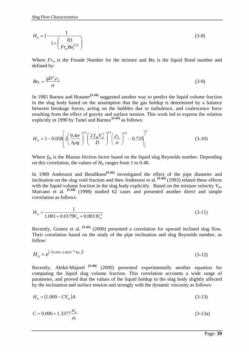
Slug Flow Characteristics

Page: 39

⎟⎟⎠

⎞⎜⎜⎝

⎛+

−=

25.0831

11

lm

ls

BoFr

H (3-8)

Where Frm is the Froude Number for the mixture and Bol is the liquid Bond number and defined by:

σρ L

lgDBo

2

= (3-9)

In 1985 Barnea and Brauner[ 3-26] suggested another way to predict the liquid volume fraction in the slug body based on the assumption that the gas holdup is determined by a balance between breakage forces, acting on the bubbles due to turbulence, and coalescence force resulting from the effect of gravity and surface tension. This work led to express the relation explicitly in 1990 by Taitel and Barnea [ 3-41] as follows:

26.04.035.0

725.024.02058.01⎥⎥⎦

⎤

⎢⎢⎣

⎡−⎟

⎠⎞

⎜⎝⎛

⎟⎟⎠

⎞⎜⎜⎝

⎛⎟⎟⎠

⎞⎜⎜⎝

⎛Δ

−=σρ

ρσ LmBs

ls DVf

gH (3-10)

Where fBs is the Blasius friction factor based on the liquid slug Reynolds number. Depending on this correlation, the values of Hls ranges from 1 to 0.48. In 1989 Andreussi and Bendiksen[ 3-42] investigated the effect of the pipe diameter and inclination on the slug void fraction and then Andreussi et al. [ 3-43] (1993) related these effects with the liquid volume fraction in the slug body explicitly. Based on the mixture velocity Vm, Marcano et al. [ 3-44] (1998) studied 62 cases and presented another direct and simple correlation as follows:

20011.00179.0001.11

mmls VV

H++

= (3-11)

Recently, Gomez et al. [ 3-45] (2000) presented a correlation for upward inclined slug flow. Their correlation based on the study of the pipe inclination and slug Reynolds number, as follow:

( )( )seHlsRe4810.245.0 10−+−= θ (3-12)

Recently, Abdul-Majeed [ 3-46] (2000) presented experimentally another equation for computing the liquid slug volume fraction. This correlation accounts a wide range of parameter, and proved that the values of the liquid holdup in the slug body slightly affected by the inclination and surface tension and strongly with the dynamic viscosity as follows:

( )ACVH mls −= 009.1 (3-13)

l

gCμμ

3377.1006.0 += (3-13a)

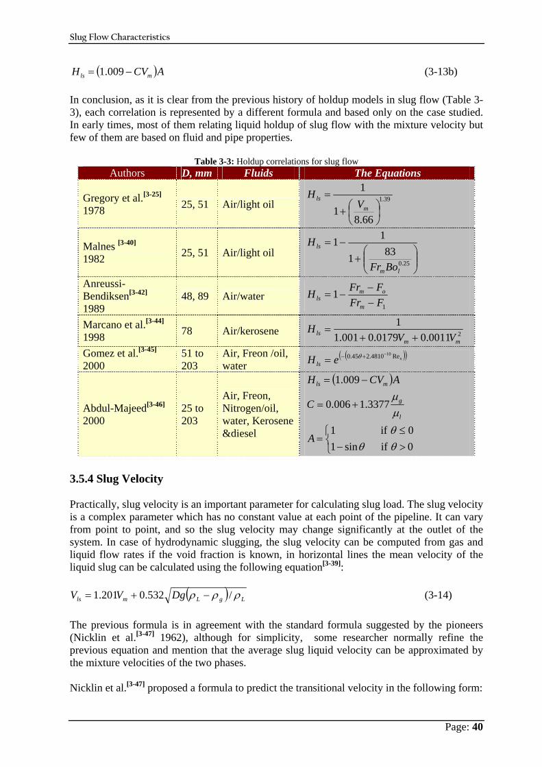
Slug Flow Characteristics

Page: 40

( )ACVH mls −= 009.1 (3-13b) In conclusion, as it is clear from the previous history of holdup models in slug flow (Table 3-3), each correlation is represented by a different formula and based only on the case studied. In early times, most of them relating liquid holdup of slug flow with the mixture velocity but few of them are based on fluid and pipe properties.

Table 3-3: Holdup correlations for slug flow Authors D, mm Fluids The Equations

Gregory et al.[ 3-25] 1978 25, 51 Air/light oil 39.1

66.81

1

⎟⎠⎞

⎜⎝⎛+

=m

lsV

H

Malnes [ 3-40] 1982 25, 51 Air/light oil

⎟⎟⎠

⎞⎜⎜⎝

⎛+

−=

25.0831

11

lm

ls

BoFr

H

Anreussi-Bendiksen[ 3-42] 1989

48, 89 Air/water 1

1FFrFFrH

m

omls −

−−=

Marcano et al.[ 3-44] 1998 78 Air/kerosene 20011.00179.0001.1

1

mmls VV

H++

=

Gomez et al.[ 3-45] 2000

51 to 203

Air, Freon /oil, water

( )( )seHlsRe4810.245.0 10−+−= θ

Abdul-Majeed[ 3-46] 2000

25 to 203

Air, Freon, Nitrogen/oil, water, Kerosene &diesel

( )

⎩⎨⎧

>−≤

=

+=

−=

0 if sin10 if 1

3377.1006.0

009.1

θθθμμ

A

C

ACVH

l

g

mls

3.5.4 Slug Velocity Practically, slug velocity is an important parameter for calculating slug load. The slug velocity is a complex parameter which has no constant value at each point of the pipeline. It can vary from point to point, and so the slug velocity may change significantly at the outlet of the system. In case of hydrodynamic slugging, the slug velocity can be computed from gas and liquid flow rates if the void fraction is known, in horizontal lines the mean velocity of the liquid slug can be calculated using the following equation[ 3-39]:

( ) LgLmls DgVV ρρρ /532.0201.1 −+= (3-14) The previous formula is in agreement with the standard formula suggested by the pioneers (Nicklin et al.[ 3-47] 1962), although for simplicity, some researcher normally refine the previous equation and mention that the average slug liquid velocity can be approximated by the mixture velocities of the two phases. Nicklin et al.[ 3-47] proposed a formula to predict the transitional velocity in the following form:

Slug Flow Characteristics

Page: 41

Dmols VVCV += (3-15) Where VD is the drift velocity of elongated bubbles in stagnant liquid, Vm is the mixture velocity and Co is a constant coefficient depending on flowing conditions and liquid properties. It is found that there is no unified value for Co in the literature for horizontal flowing. Gregory-Scott[ 3-30] found Co = 1.35. Mattar-Gregory[ 3-48] proposed 1.32. Dukler-Hubbard[ 3-23] suggested an equation to calculate Co in their model and the range was 1.25 to 1.28. Singh-Griffith[ 3-49] value was 0.95. Ferre[ 3-50] reported a range from 1.02 to 1.3 for a 50 m long pipe. Bendiksen[ 3-51] related the Co value with critical Froude number which was equal to 3.5; Co = 1.05 if Fr < 3.5 and Co = 1.2 if Fr > 3.5 for horizontal pipeline. Like Bendiksen[ 3-51], Theron[ 3-52] related Co value with Froude number and suggested 1.3 for Co for general use. Wang et al. [ 3-53] as well as some of the previous researchers[ 3-51, 3-52] related Co value with the Froude number and found Co value is 1.373 in their experimental study in horizontal flow pipelines. Moreover, Wang et al. [ 3-53] attributed the discrepancies between the researchers in calculating Co value as measuring the transitional velocity at different location in pipelines. Wang et al. [ 3-53] value measured at x/D = 1157 for Fr > 3.5 and interestingly, if Fr < 3.5 it is shown Co does not depend on x/D and approximately equals to the value measured from single bubble moving in constant liquid flow. In 2008, Ragab-Brandstaetter[ 3-54] proposed a new correlation based on CFD simulation results for determination of the average slug velocity in small diameter horizontal pipelines. Their correlation relates the slug mean velocity with the mixture velocity of the fluids as follows:

298.05307.1 += mls V V (3-16) From all of the above, it can be concluded that a lot of work in the past was devoted to experimental determination of slug parameters. However, no universal correlation to determine slug flow characteristics could be found so far. For this reason within this thesis an attempt is made to assess slugging phenomena in a more fundamentally based view by using Computational Fluid Dynamics (CFD). In that follows first the underlying mathematical and physical fundamental is presented.

3.6 Nomenclature

A Pipe cross-sectional area Bol Liquid Bond number Co Constant coefficient

D, d Pipe diameter fBs Blasius friction factor Fr Froude number

Frm Froude number for the mixture flow Fsl, Fs, fs, fr Slug frequency

g Gravitational constant Hle Equilibrium stratified liquid holdup

Slug Flow Characteristics

Page: 42

Hs, Hls Liquid slug holdup L Pipe line length

Ls Slug length Lsr Reference slug length at the end of the tested pipe section P Pressure

Res Slug Reynolds number Ug Gas velocity VD Drift velocity Vls Slug velocity

Vm, Um Mixture velocity Vsl, Usl Superficial liquid velocity

ρ Liquid density σ Interfacial tension

θ, β Pipe inclination ρg Gas density

μg, μl Gas and liquid viscosity respectively ρL Liquid density

3.7 References

3-1. Campbell, J. M.: Gas Conditioning and Processing: Volume 1: The Basic Principles, 8th Edition, 2nd Printing, John M. Campbell and Company, Norman, Oklahoma, USA, 2001.

3-2. Taitel, Y. and Dukler, A. E.: “A Model for Prediction Flow Regime Transitions in Horizontal and near Horizontal Gas-Liquid Flow,” AIChE J., Vol. 22, Pages 47-55, 1976.

3-3. Taitel, Y.: “Stability of Severe Slugging,” International Journal of Multiphase Flow, Vol. 12, No. 2, Pages 203-207, 1986.

3-4. Miyoshi, M., Doty, D. R. and Schmidt, Z.: “Slug-Catcher Design for Dynamic Slugging in an Offshore Production Facility,” SPE Paper 14124 & SPE Production Engineering, Pages 563-573, Nov. 1988.

3-5. Huntley, A. R. and Silvester, R. S.: “Hydrodynamic Analysis Aids Slug Catcher Design,” Oil & gas J., Vol. 81, No. 38, Pages 95-100, Sept. 19, 1983.

3-6. Bos, A. and du Chatinier, J. G.: “Simulation of Gas/Liquid Flow in Slug Catchers,” SPE Paper 13724 & SPE Production Engineering, Pages 178-182, August 1987.

3-7. Genceli, H., Kuenhold, K. A. and Brill, J. P.: “Dynamic Simulation of Slug Catcher Behaviour,” SPE Paper 18235, Presented at the 63rd Annual Technical Conference and Exhibition of SPE held in Houston, Texas, Oct.2-5, 1988.

3-8. Burke, N. E. and Kashou, S. F.: “Slug-Sizing/Slug-Volume Prediction: State of the Art Review and Simulation,” SPE 30902 & SPE Production & Facilities, Pages 166-172, August 1996.

3-9. Kovalev, K., Cruickshank, A. and Purvis, J.: “The Slug Suppression System in Operation,” SPE Paper 84947, Presented at Offshore Europe 2003 held in Aberdeen, UK, 2-5 Sept. 2003.

3-10. Yocum, B. T.: “Offshore Riser Slug Flow Avoidance: Mathematical Models for Design and Optimization,” SPE 4312, Presented at SPE European Meeting held in London, England, April 2-3, 1973.

3-11. Cady, P. D.: “How to Stop Slug Flow in Condenser Outlet Piping,” Hydrocarbon Proc. Pet. Ref. Vol. 42 (9), Page 192, Sept. 1963.

Slug Flow Characteristics

Page: 43

3-12. Havre, K. and Dalsmo, M.: “Active Feedback Control as the Solution to Severe Slugging,” SPE Paper 71540, Presented at the 2001 SPE Annual Technical Conference and Exhibition held in New Orleans, Louisiana, 30 Sept.-3 Oct. 2001.

3-13. Schmidt, Z., Brill, J. P. and Beggs, H. D.: “Experimental Study of Severe Slugging in a Two-Phase-Flow Pipeline-Riser Pipe System,” Society of Petroleum Engineers Journal, Pages 407-414, Oct. 1980.

3-14. Hill, T. J., Fairhurst, C. P. and Nelson, C. J.: “Multiphase Production Through Hilly Terrain Pipelines in Cusiana Oilfield, Colombia,” SPE Paper 36606, Presented at 1996 SPE Annual Technical Conference and Exhibition held in Denver, Colorado, USA, 6-9 Oct. 1996.

3-15. Brill, J. P., Schmidt, Z., Coberly, W. A., Herring, J. D. and Moore, D. W.: “Analysis of Two-Phase Testes in Large-Diameter Flow Lines in Prudhoe Bay Field,” SPEJ, Pages 363-378, June 1981.

3-16. Manolis, I. G., Mendes-Tatsis, M. A. and Hewitt, G. F.: “Average Length of Slug Region, Film Region, and Slug Unit in High-Pressure Gas-Liquid Slug Flow,” Int. Conference on Multiphase Flow (ICMF), Lyon, 1998.

3-17. Scott, S. L., Shoham, O. and Brill, J. P.: “Prediction of Slug Length in Horizontal Large-Diameter Pipes,” SPE Paper 15103 & SPE Production Engineering, Vol. 4, issue 3, Pages 335-340, August 1989.

3-18. Hill, T. J. and Wood, D. G.: “Slug Flow: Occurrence, Consequences and Prediction,” SPE Paper 27960, Presented at The University of Tulsa Centennial Petroleum Engineering Symposium held in Tulsa, OK, USA, Pages 53-62, 29-31 August 1994.

3-19. Al-Safran, E. M., Taitel Y. and Brill, J. P.: “Prediction of Slug Length Distribution along a Hilly Terrain Pipeline Using Slug Tracking Model,” Transactions of the ASME, Journal of Energy Resources Technology, Vol. 126, Pages 54-62, March 2004.

3-20. Al-Safran, E. M., Sarica, C., Zhang, H. Q. and Brill, J. P.: “Probabilistic/Mechanistic Modeling of Slug-Length Distribution in a Horizontal Pipeline,” SPE Paper 84230 was first Presented at the 2003 SPE Annual Technical Conference and Exhibition, Denver, 5-8 Oct., and revised and published also at SPE Production & Facilities, Pages 160-172, May 2005.

3-21. Bernlcot, M. F. and Drouffe, J. M.: “A Slug-Length Distribution Law for Multiphase Transportation System,” SPE Paper 17864 & SPE Production Engineering, Pages 166-170, May 1991.

3-22. Omgba-Essama, C.: Numerical Modelling of Transient Gas-Liquid Flows (Application to Stratified & Slug Flow Regimes), PhD Thesis, Cranfield University, School of Engineering, applied Mathematics and Computing Group, April 2004.

3-23. Dukler A. E. and Hubbard M. G.: “A Model for Gas-Liquid Slug Flow in Horizontal and near Horizontal Tubes”, Ind. Eng. Chem. Fundamental, Vol. 14, No. 4, Pages 337-347, 1975.

3-24. Nicholson M. K., Aziz K. and Gregory G. A.: “Intermittent Two-Phase Flow in Horizontal Pipes: Predictive Models,” Canadian Journal of Chemical Engineering, Vol. 56, Pages 653-663, 1978.

3-25. Gregory G. A., Nicholson M. K. and Aziz K.: “Correlation of the Liquid Volume Fraction in the Slug for Horizontal Gas-Liquid Slug Flow”, International Journal of Multiphase Flow, Vol. 4, No. 1, Pages 33-39, 1978.

3-26. Barnea D. and Brauner N.: “Holdup of the Liquid Slug in Two-Phase Intermittent Flow,” International Journal of Multiphase Flow, Vol. 11, No.1, Pages 43-49, 1985.

Slug Flow Characteristics

Page: 44

3-27. Andreussi P., Paglianti A., Vatistas N., Minervini A. and Bendiksen K.: “Analysis of Slug Flow in near Horizontal and Horizontal Pipes,” European Two-Phase Flow Group Meeting, Brussels, Belgium, Paper B2, 30 May to 1 June 1988.

3-28. Nydal, O. J., Pintus, S. and Andreussi, P.: “Statistical Characterization of Slug Flow in Horizontal Pipes,” International Journal of Multiphase Flow, Vol. 18, No. 3, Pages 439-453, 1992.

3-29. Manolis, I. G.: High Pressure Gas-Liquid Slug Flow, PhD Thesis, Department of Chemical Engineering and Chemical Technology, Imperial College of Science, Technology & Medicine, UK, 1995.

3-30. Gregory G. A. and Scott D. S.: “Correlation of Liquid Slug Velocity and Frequency in Horizontal Co-Current Gas-Liquid Slug Flow,” AIChE Journal, Vol. 15, No. 6, Pages 933-935, 1969.

3-31. Taitel Y. and Dukler A. E.: “A Model for Slug Frequency During Gas-Liquid Flow in Horizontal and Near Horizontal Pipes,” International Journal of Multiphase Flow, Vol. 3, No. 6, Pages 585-596, 1977.

3-32. Heywood, N. I. and Richardson, J. F.: “Slug Flow of Air-Water Mixtures in a Horizontal Pipe: Determination of Liquid Holdup by Gamma-Ray Absorption,” Chemical Engineering Science, Vol. 34, Pages 17-30, 1979.

3-33. Tronconi E.: “Prediction of Slug Frequency in Horizontal Two-Phase Slug Flow”. AIChE Journal, Vol. 36, No. 5, Pages 701-709, 01 May 1990.

3-34. Hill, T. J. and Wood, D. G.: “A New Approach to the Prediction of Slug Frequency,” SPE 20629, 65th Annual Technical Conference and Exhibition of the Society of Petroleum Engineers held in New Orleans, LA, USA, September 23-26, 1990.

3-35. Stapelberg, H. H. and Mewes, D.: “The Pressure Loss and Slug Frequency of Liquid-Liquid-Gas Slug Flow in Horizontal Pipes,” International Journal of Multiphase Flow, Vol. 20, No. 2, Pages 285-303, 1994.

3-36. Zabaras, G. J.: “Prediction of Slug Frequency for Gas Liquid Flows,” SPE Paper 56462, Presented at the 1999 SPE Annual Technical Conference and Exhibition held in Houston, Texas, 3-6 October 1999.

3-37. Crowley, C. J., Barry, J. J. and Rothe, P. H.: Design Manual for Multiphase Gas and Oil pipelines, CREARE Report PR-172-904 Prepared for the American gas association, Hanover, NH, 1989.

3-38. Greskovich, E. J. and Shrier, A. L.: “Slug Frequency in Horizontal Gas-Liquid Slug Flow,” Industrial and Engineering Chemistry Process Design and Development, Vol. 11, No. 2, Pages 317-318, 1972.

3-39. Wei: Review and Guidelines of Dynamic Models: OLGA, TACITE, ProFES Transient for Multiphase Pipeline Applications,” Technical Report ABB, No. SECRC/B/TR-2000/099E, Sweden, 2000, http://www.abb.com/cawp/seitp161/ 2cfdabece457886841256f500041089e.aspxlink.

3-40. Malnes, D.: Slug Flow in Vertical, Horizontal and Inclined Pipes, Report IFE/KR/E-83/002, V. Inst. for Energy Technology Flow, Vol. 1, Page 537.

3-41. Taitel, Y. and Barnea, D.: “Effect of Gas Compressibility on a Slug-Tracking Model,” Chemical Eng. Science, Vol. 53, Pages 2089-2097, 1998.

3-42. Andreussi, P. and Bendiksen, K.: “An Investigation of Void Fraction in Liquid Slugs for Horizontal and Inclined Gas-Liquid Pipe Flow,” International Journal of Multiphase flow, Vol. 15, Issue 6, Pages 937-946, November 1989

3-43. Andreussi, P., Bendiksen, K. H. and Nydal, O. J.: “Void Distribution in Slug Flow,” International Journal of Multiphase Flow, Vol. 19, Issue 5, Page 817-828, 1993.

Slug Flow Characteristics

Page: 45

3-44. Marcano, R., Chen, X. T, Sarica, C. and Brill, J. P.: “A Study of Slug Characteristics for Two-Phase Horizontal Flow,” SPE 39856, Presented at the 1998 International Petroleum Conference and Exhibition held in Villahermosa, Mexico, 3-5 March 1998.

3-45. Gomez, L. E., Shoham, O. and Taitel, Y.: “Prediction of Slug Liquid Holdup: Horizontal to Upward Vertical Flow,” International Journal of Multiphase Flow, Vol. 26, Pages 517-521, 2000.

3-46. Abdul-Majeed, G. H.: “Liquid Slug Holdup in Horizontal and Slightly Inclined Two-Phase Slug Flow,” Journal of Petroleum Science and Engineering, Vol. 27, No. 1-2, Pages 27-32, 2000.

3-47. Nicklin, D. J., Wilkes, J. O. and Davidson, J. F.: “Two-Phase Flow in Vertical Tubes,” Trans. Inst. Chem. Eng., Vol. 40, Pages 61-68, 1962.

3-48. Mattar, L. and Gregory, G. A.: “Air-Oil Slug Flow in an Upward-Inclines Pipe-I: Slug Velocity, Holdup and Pressure Gradient,” J. Can. Petr. Tech., Vol. 13, Pages 69-76, 1974.

3-49. Singh, G. and P. Griffith, P.: Down Sloping Inclined Pipe Pressure Drop and Holdup, ASME Report 76-Pet-29, 1976.

3-50. Ferre, D.: “ Ecoulements diphasiques a poches en conduite horizontale,” Rev. Inst. Fr. Pet., Vol. 34, Pages 113-142, 1979.

3-51. Bendiksen, K. H.: “An Experimental Investigation of the Motion of the Long Bubbles in Inclined Tubes,” International Journal of Multiphase Flow, Vol. 10, Issue 4, Pages 476-483, 1984.

3-52. Theron, B.: Ecoulements instationnaires intermittents de gaz et de liquide en conduite horizontale, These Inst. Natl. Polytech, Toulouse, 1989.

3-53. Wang, X., Guo, L. and Zhang, X.: “An Experimental Study of the Statistical Parameters of Gas-liquid Two-Phase Slug Flow in Horizontal Pipeline,” International Journal of Heat and Mass Transfer, Vol. 50, No. 11-12, Pages 2439-2443, June 2007.

3-54. Ragab, A., Brandstätter, W. and Shalaby, S.: “CFD-Simulation of Multiphase Flows in Horizontal and Inclined Pipelines,” Oil and Gas European Magazine, Vol. 1, Pages 34-40, 2008.

CFD for Multiphase Flow VOF Method

Page: 46

CHAPTER IV

Computational Fluid Dynamics for

Multiphase Flow

The Volume of Fluid Method (VOF)

4.1 Introduction In this chapter the mathematical model of transport processes that can be simulated with volume of fluid (VOF) is presented. It includes the mass, momentum and energy balance equations in integral form, constitutive relations required for the problem closure, models of turbulence in fluid flow, and boundary conditions. The theoretical considerations in this chapter are conducted in a symbolic coordinate free notation which directly conveys the physical meaning of particular terms without (unnecessary) reference to any coordinate system. It largely follows COMET user manual[ 4-1].

4.2 General Governing Equations The behaviour of continuum is governed by the so-called transport equations[ 4-2] based on the following basic laws of physics expressing balance (conservation) of:

Mass Momentum Energy

The most general way of writing equations expressing these laws[ 4-3, 4-4, 4-5, 4-6 4-7] is in integral form valid for an arbitrary part of the continuum of volume V bounded by surface S as shown in Figure 4-1. 4.2.1 Mass Balance Equation The equation expressing the mass conservation law, known as the continuity equation, can be written as follows:

( ) 0. =−+ ∫∫ ds vvdV dtd

S sVρρ (4-1)

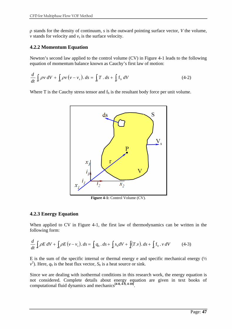
CFD for Multiphase Flow VOF Method

Page: 47

ρ stands for the density of continuum, s is the outward pointing surface vector, V the volume, v stands for velocity and vs is the surface velocity. 4.2.2 Momentum Equation Newton’s second law applied to the control volume (CV) in Figure 4-1 leads to the following equation of momentum balance known as Cauchy’s first law of motion:

( ) ∫ ∫∫∫ +=−+S V bS sV

dV ds Tds vv vdV vdtd f..ρρ (4-2)

Where T is the Cauchy stress tensor and fb is the resultant body force per unit volume.

Figure 4-1: Control Volume (CV).

4.2.3 Energy Equation When applied to CV in Figure 4-1, the first law of thermodynamics can be written in the following form:

( ) ( ) ∫∫ ∫ ∫∫∫ +++=−+V bS V shhS sV

dV v ds vTdVds qds vv EdV Edtd .f..s..ρρ (4-3)

E is the sum of the specific internal or thermal energy e and specific mechanical energy (½ v2). Here, qh is the heat flux vector, Sh is a heat source or sink. Since we are dealing with isothermal conditions in this research work, the energy equation is not considered. Complete details about energy equation are given in text books of computational fluid dynamics and mechanics[ 4-8, 4-9, 4-10].

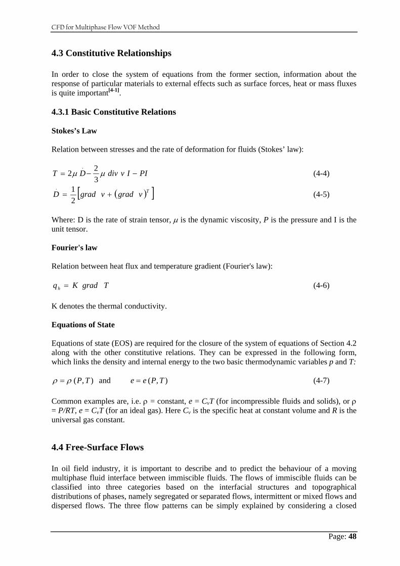
CFD for Multiphase Flow VOF Method

Page: 48

4.3 Constitutive Relationships In order to close the system of equations from the former section, information about the response of particular materials to external effects such as surface forces, heat or mass fluxes is quite important[ 4-1]. 4.3.1 Basic Constitutive Relations Stokes’s Law Relation between stresses and the rate of deformation for fluids (Stokes’ law):

PII v div DT −−= μμ322

. (4-4)

( )[ ]Tv gradv gradD +=21.

(4-5)

Where: D is the rate of strain tensor, μ is the dynamic viscosity, P is the pressure and I is the unit tensor. Fourier's law Relation between heat flux and temperature gradient (Fourier's law):

T grad Kqh = (4-6) K denotes the thermal conductivity. Equations of State Equations of state (EOS) are required for the closure of the system of equations of Section 4.2 along with the other constitutive relations. They can be expressed in the following form, which links the density and internal energy to the two basic thermodynamic variables p and T:

),(and ),( T P ee T P == ρρ (4-7) Common examples are, i.e. ρ = constant, e = CvT (for incompressible fluids and solids), or ρ = P/RT, e = CvT (for an ideal gas). Here Cv is the specific heat at constant volume and R is the universal gas constant.

4.4 Free-Surface Flows In oil field industry, it is important to describe and to predict the behaviour of a moving multiphase fluid interface between immiscible fluids. The flows of immiscible fluids can be classified into three categories based on the interfacial structures and topographical distributions of phases, namely segregated or separated flows, intermittent or mixed flows and dispersed flows. The three flow patterns can be simply explained by considering a closed

CFD for Multiphase Flow VOF Method

Page: 49

container partially filled with a liquid phase, with the other part occupied by a gas phase. The first class occurs when the container is oscillating very gently with a low amplitude and frequency and the two phases remain separated with a single well defined interface. Intermittent or mixed flow occurs when the frequency and amplitude are increased to the extant that the waves become unstable and break. Part of the interface breaks up and small bubbles are trapped in the liquid or small liquid drops are present in the gas zone. Dispersed flows occur when the container is shaken vigorously so that gas and liquid mix to form a suspension. Methods used for predictions of free-surface flows fall into two broad classes: front tracking and front capturing approaches. Both of them are available in the FLUENT–VOF[ 4-11, 4-12] tracking model. 4.4.1 Front-Tracking Approach Strictly speaking, the continuum concept does not hold across the free surface, since in general, fluid physical properties do not change continuously across it. However, the fact that fluids involved do not mix, allows us to use the general governing equations as they stand for each fluid separately. To do this, the solution domain is to be subdivided into a number of sub-domains, each containing one fluid only. The interface between sub-domains determines the free surface. This well defined interface is a dynamic surface not static, so it changes its shape and position due to changing flow conditions and a continuous interaction between the sub-domains. This implies that simulation of free-surface flows using front-tracking method inevitably involves domains with moving boundaries. The following two conditions determine the shape of the free surface and the forces exerted on fluids in contact[ 4-8]:

The kinematic condition, states that there is no convective mass transfer through the free surface, or in other words that the fluid velocity component normal to the free surface is equal to the free surface velocity, i.e.: ( )[ ] 0n. fs =− vv s (4-8)

fs stands for the part of the boundary that coincides with the free surface. The dynamic condition, states that the forces acting on fluids in contact at the free surface are in equilibrium. In the absence of surface-tension effects, this condition reduces to the statement that the stresses in fluid on both sides of the free surface in its immediate vicinity are equal. If a further assumption is made that viscous effects are negligible as it is often the case, the dynamic condition reduces to the statement that the pressures on either side of the interface are equal.

The advantage of this approach is that the interface position is known throughout the calculation and it remains very sharp. This also facilities the effort needed for the calculation of the interface curvature and its subsequent implementation for the inclusion of the surface-tension force. However, when the flow conditions are such that free-surface is strongly enfolded and the number of sub-domains containing one fluid only is not constant all the time (as in slug, plug and dispersed flows), the tracking of the interface becomes very complex and its accurate numerical implementation very expensive.

CFD for Multiphase Flow VOF Method

Page: 50

4.4.2 Front-Capturing Approach Front-capturing methods require a kind of a two-phase model. Immiscible fluids are then not considered separately, but are rather replaced by an effective fluid which is considered as a continuum in the entire solution domain. The physical properties of the effective fluid based on physical properties of constituent fluids (e.g. liquid [l] and gas [g]) and a scalar indicator function, known as volume fraction C, according to the following expressions:

( ) gl CC ρρρ −+= 1 (4-9)

( ) gl CC μμμ −+= 1 (4-10) Where:

The subscripts l and g stand for the liquid and gas respectively. The function C is used to distinguish between two different fluids. A value of unity indicates the presence of liquid phase and the value of zero indicates the presence of gas phase. Volume fraction values between these two limits indicate the presence of the interface.

The volume faction C and the mass fraction c of liquid phase are linked by the expression:

ρρ lCc = (4-11)

It is assumed that for the portion of solution domain where c has a value between 1 and 0, both liquid and gas phases share the same velocity, pressure and temperature. In this way, this free-surface capturing model reduces to modeling of multiphase flows. The fact that the method assumes that both fluids share the same velocity, pressure and temperature field makes it suitable and accurate for stratified and slug flows. In parts of the solution domain where only one fluid is present, this assumption is irrelevant since all transport equations are identical as in the case of single flow and the approximation is made only in a small part of the solution domain where the interface exists. For dispersed flows this assumption is too crude, and the method should be used with much more precaution. In order to model the two fluids as a continuum by using governing equations, the density (ρ) should be continuous and differentiable over the whole flow domain. For the calculation of the interface curvature, the requirement on the smoothness of C is even more stringent, requiring being twice differentiable. A possible way to accomplish this is to give the transitional area between the two fluids, which is in reality a discontinuous step, a small finite thickness δfs. A numerical implementation of the method introduces certain amount of numerical diffusion, which gives always the finite transitional area. If a non-diffusive discretization is used, than transition area can be obtained by a suitable smoothing of the field of C.

4.5 Turbulence Modelling Most multiphase fluid flows in oil field are in a particular state of continuous instability, called turbulence, and can be said to be steady on an average basis only, since small scale,

CFD for Multiphase Flow VOF Method

Page: 51

high frequency fluctuations of all the flow quantities, in both space and time, are always present. A flow exhibiting these macroscopic fluctuations is called turbulent flow. Otherwise, a well ordered flow, free of macroscopic fluctuations is called laminar flow. The turbulent flow is well described by the governing equations of first section of this chapter with Stokes and Fourier laws (Section 4.2.1) as constitutive relations. Further details on turbulence modelling are given in different books[ 4-13, 4-14, 4-15] However, their numerical solution (direct numerical simulation, DNS) requires a mesh with spacing smaller than the length scale of the smallest turbulent eddies, and time steps smaller than the smallest time scale of turbulent fluctuations. Alternatives are Large Eddy Simulation (LES) [ 4-7, 4-10], in which only the largest unsteady motions are resolved and the rest is modelled, and the solution of Reynolds Averaged Navier-Stokes (RANS) equations, where all turbulent effects on the mean flow are modelled as functions of mean fluid flow quantities. 4.5.1 Reynolds Averaged Navier-Stokes (RANS) Equations The RANS equations are obtained by using a statistical description of turbulent motion, formulated in terms of averaged quantities. Each dependent variable is expressed as the sum of its mean, or time averaged value φ , and a fluctuating component φ″ :

φφφ ′′+= (4-12) Where:

( ) ( ) ξξφτ

φτ

τ d t r t r ∫− += 2

2

,1, (4-12a)

The time interval τ is large enough with respect to the time scale of the turbulent fluctuations, but small with respect to the scale of other time dependent effects. For compressible flows this averaging leads to products between the density and fluctuations of other variables such as velocity or internal energy. In order to avoid their explicit occurrence, a density-weighted (Favre) averaging is introduced through the following definition:

ρρφφ =ˆ (4-13)

With

0,ˆ =′′+= φρφφφ and (4-13a) For constant density flows (ρ =Constant), φφ ˆ= and φφ ′=′′ . Applied to the governing equations, the following equations for mass, energy and momentum balance in turbulent flows are obtained:

( ) 0. =−+ ∫∫ S sVds vv dV

dtd ρρ (4-14)

CFD for Multiphase Flow VOF Method

Page: 52

( ) ( ) ∫∫∫∫ +′′−=−+V cS icS siV i dV Sds vc qds vv c dV c

dtd

ii.. ρρρ (4-15)

( ) ( ) ∫∫∫∫ +′′−=−+V bSS sV

dV ds vv Tds vv v dV v dtd f.. ρρρ (4-16)

( ) ( ) ∫∫∫∫∫ ++′′−=−+VV hS hS sV

dV v gradTdV ds ve qds vv e dV e dtd :S.. ρρρ (4-17)

In the above expressions and in what follows, the averaging signs (over-bar and hat) are retained only for averages involving products of fluctuating quantities and all dependent variables are considered as averaged quantities (density and pressure as time averages and velocity and internal energy as density-weighted averages). It can be seen that the averaged continuity Equation 4-14 remains the same as the instantaneous one (Equation 4-1). However, the averaging procedure produces a set of new unknowns in the phases, momentum and energy conservation equations, respectively: Turbulent mass flux:

vc q itc i

′′−= ρ (4-18) Turbulent momentum flux, Reynolds stress:

vv T t ′′−= ρ (4-19) Turbulent heat flux:

ve q ith ′′−= ρ (4-20)

Since these quantities are unknown, the averaged Equations 4-14 to 4-17 are accompanied by the so-called turbulence models, which provide these unknowns by expressing the correlations of the fluctuations in terms of the mean quantities. To do so, one has to rely on experimental data and knowledge obtained from DNS. No single model can be expected to reproduce well the effects of turbulence on the mean flow in all practical applications. The most popular turbulence models are eddy-viscosity models, which postulate an analogy between the turbulent and viscous diffusion (Boussinesq eddy-viscosity hypothesis) and model the effects of turbulence by introducing turbulent diffusivity and viscosity coefficients:

( )

T grad q

Iv div DT

c grad Dq

tth

ttt

ititc i

κ

ρκμμ

ρ

≈

+−≈

≈

322

,

& (4-21)

CFD for Multiphase Flow VOF Method

Page: 53

where: Di,t,μt and κt represent the turbulent diffusivity coefficients and κ stands for the turbulent kinetic energy. These coefficients are non-linear functions of the flow parameters and usually vary several orders of magnitude within the flow region. 4.5.2 The Standard κ-ε Model The standard κ-ε model is the most widely used eddy-viscosity model. It can be summarised as follows. In Equations 4-4 and 4-6; Di,μ and κ are replaced by their so-called effective values:

teff

teff

tiieffi DDD

κκκ

μμμ

+=

+=

+= ,,

(4-22)

Where:

ρDi,t, μt and κt are the turbulent mass diffusivity, viscosity and conductivity, defined as:

T

Pttt

c

tti

C C Di

σμκ

εκρμ

σμρ μ === ,,

2

, (4-23)

σci Cμ and σT are empirical coefficients which presented in Table 4-1 and κ stands for the kinetic energy of turbulence and ε for its dissipation rate. Note that in the case of a multiphase fluid flow all turbulent Schmidt numbers σci should be given identical values if the continuity equation is to be exactly satisfied. The pressure P is replaced by the so-called modified pressure:

( )κρμ v div PP tm ++=32 (4-24)

The kinetic energy of turbulence κ and its dissipation rate ε are defined as:

( )Tv grad: v grad v . v ′′=′′=ρμεκ ,

21 (4-25)

and are obtained by solving their respective transport equations:

( ) ( )∫ ∫∫∫ −++=−+S V BkS sV

dV PPds qds vv dV dtd ρεκρκρ .. (4-26)

( )

( )∫ ∫

∫∫

⎟⎟⎠

⎞⎜⎜⎝

⎛−+−+

=−+

S V B

S sV

dV v div CP max CCPCds q

ds vv dV dtd

ρεκε

κερ

κε

ερερ

ε 43

2

2

2

1 0,.

. (4-27)

Where the diffusion fluxes for κ and ε are defined as:

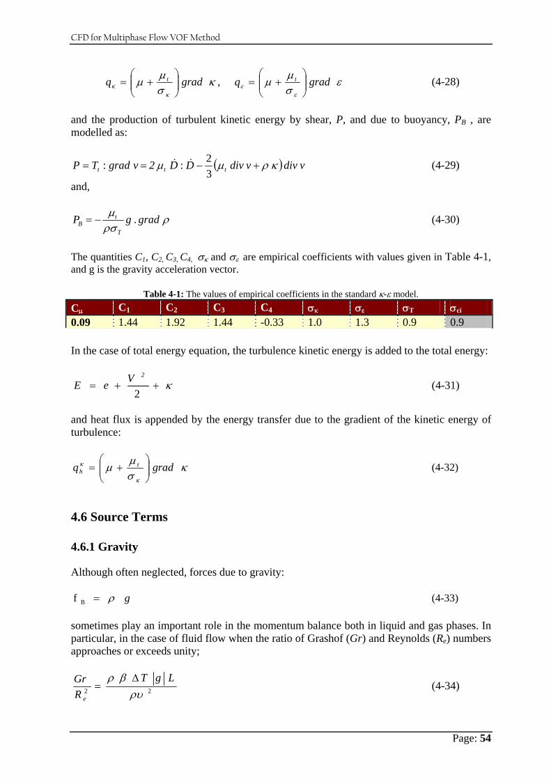
CFD for Multiphase Flow VOF Method

Page: 54

εσμμκ

σμμ

εε

κκ grad q , grad q tt

⎟⎟⎠

⎞⎜⎜⎝

⎛+=⎟⎟

⎠

⎞⎜⎜⎝

⎛+= (4-28)

and the production of turbulent kinetic energy by shear, P, and due to buoyancy, PB , are modelled as:

( ) v div v div DD 2 v gradTP ttt κρμμ +−==32:: && (4-29)

and,

ρρσμ grad . gP

T

tB −= (4-30)

The quantities C1, C2, C3, C4, σκ and σε are empirical coefficients with values given in Table 4-1, and g is the gravity acceleration vector.

Table 4-1: The values of empirical coefficients in the standard κ-ε model. Cμ C1 C2 C3 C4 σκ σε σT σci 0.09 1.44 1.92 1.44 -0.33 1.0 1.3 0.9 0.9 In the case of total energy equation, the turbulence kinetic energy is added to the total energy:

κ++=2

2V eE (4-31)

and heat flux is appended by the energy transfer due to the gradient of the kinetic energy of turbulence:

κσμμκ

κ grad q th ⎟⎟

⎠

⎞⎜⎜⎝

⎛+= (4-32)

4.6 Source Terms 4.6.1 Gravity Although often neglected, forces due to gravity:

g ρ=Bf (4-33) sometimes play an important role in the momentum balance both in liquid and gas phases. In particular, in the case of fluid flow when the ratio of Grashof (Gr) and Reynolds (Re) numbers approaches or exceeds unity;

22 ρυβρ L g T

RGr

e

Δ= (4-34)

CFD for Multiphase Flow VOF Method

Page: 55

Forces due to a non-uniform density field are then significant, and the buoyancy force has to be considered. Conveniently, it is written in the following way:

( ) g g refrefB ρρρ +−=f (4-35) Here, ΔT, L and v are characteristic temperature difference, length and velocity, respectively, and g is the acceleration due to gravity. Usually, the first part of Equation 4-35 is retained as a part of the body force, while the second part is included in the modified pressure:

r . g ........ P refm ρ−= (4-36) If ρref is used instead of ρ in all other terms of the governing equations, then this leads to the so-called Boussinesq approximation for buoyant flows. It can be used when temperature differences are relatively small. The strength of buoyancy induced flow is measured by the Rayleigh (Ra) number:

κμρβ

C L g T

Pr Gr Ra P23Δ

== (4-37)

For Ra < 108 buoyant flow is laminar, and the transition to turbulence occurs at 108 < Ra < 1010. 4.6.2 Surface Tension The surface tension force is a tensile force tangential to the interface separating two fluids, which tries to keep the fluid molecules at the free boundary in contact with the rest of the fluid. Its magnitude depends strongly on the nature of the two fluids and temperature. It is especially important at an interface between liquid and gas. For a curved interface the surface tension results in a force normal to the interface fσ,n as depicted in Figure 4-2 while the tangential effects cancel out if the surface tension coefficient σ is constant:

sf,tfnf , s

t , K s,t,n ∂

∂=

∂∂

==σσσ σσσ (4-38)

where n, t and s are unit vectors in the local orthogonal coordinate system (n, t, s) at the free surface (n is normal to the free surface and directed from liquid to gas, as shown in Figure 4-2) and K is the mean curvature of the free-surface:

st RRK 11

+= (4-39)

Rt and Rs being principal radii of curvature of the surface. If the fluids are in equilibrium, the normal component fσ,n is balanced by a pressure jump across the interface–otherwise the interface will accelerate.

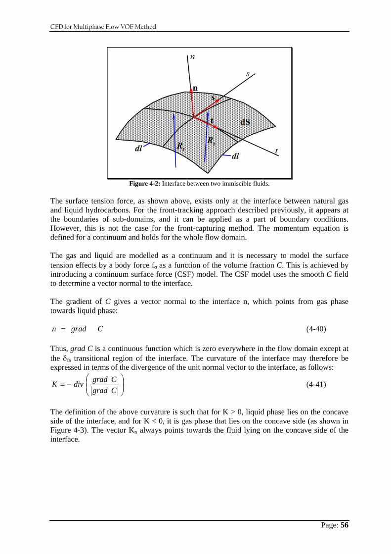
CFD for Multiphase Flow VOF Method

Page: 56

Figure 4-2: Interface between two immiscible fluids.

The surface tension force, as shown above, exists only at the interface between natural gas and liquid hydrocarbons. For the front-tracking approach described previously, it appears at the boundaries of sub-domains, and it can be applied as a part of boundary conditions. However, this is not the case for the front-capturing method. The momentum equation is defined for a continuum and holds for the whole flow domain. The gas and liquid are modelled as a continuum and it is necessary to model the surface tension effects by a body force fσ as a function of the volume fraction C. This is achieved by introducing a continuum surface force (CSF) model. The CSF model uses the smooth C field to determine a vector normal to the interface. The gradient of C gives a vector normal to the interface n, which points from gas phase towards liquid phase:

Cgradn = (4-40) Thus, grad C is a continuous function which is zero everywhere in the flow domain except at the δfs transitional region of the interface. The curvature of the interface may therefore be expressed in terms of the divergence of the unit normal vector to the interface, as follows:

⎟⎟⎠

⎞⎜⎜⎝

⎛−=

C gradC grad div K (4-41)

The definition of the above curvature is such that for K > 0, liquid phase lies on the concave side of the interface, and for K < 0, it is gas phase that lies on the concave side (as shown in Figure 4-3). The vector Kn always points towards the fluid lying on the concave side of the interface.

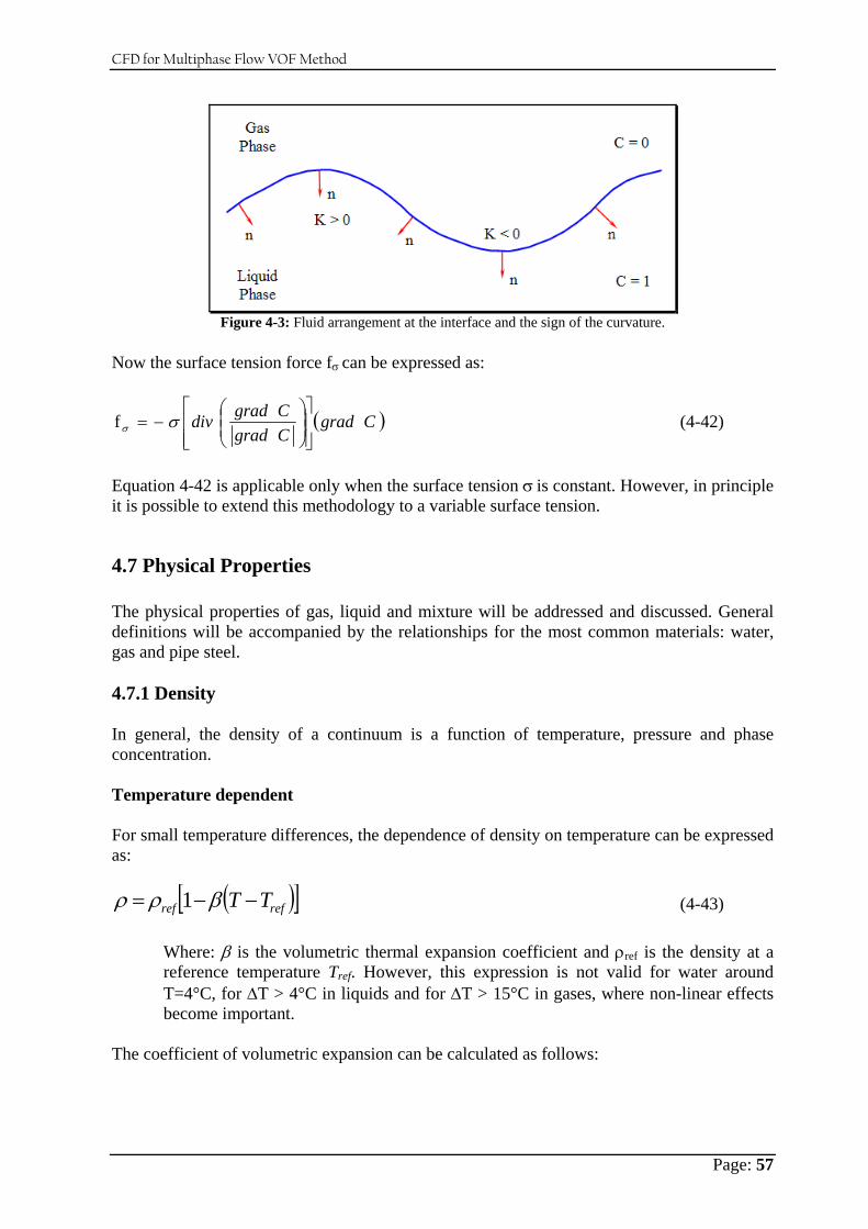
CFD for Multiphase Flow VOF Method

Page: 57

Figure 4-3: Fluid arrangement at the interface and the sign of the curvature.

Now the surface tension force fσ can be expressed as:

( )C gradC gradC grad div

⎥⎥⎦

⎤

⎢⎢⎣

⎡⎟⎟⎠

⎞⎜⎜⎝

⎛−= σσf (4-42)

Equation 4-42 is applicable only when the surface tension σ is constant. However, in principle it is possible to extend this methodology to a variable surface tension.

4.7 Physical Properties The physical properties of gas, liquid and mixture will be addressed and discussed. General definitions will be accompanied by the relationships for the most common materials: water, gas and pipe steel. 4.7.1 Density In general, the density of a continuum is a function of temperature, pressure and phase concentration. Temperature dependent For small temperature differences, the dependence of density on temperature can be expressed as:

( )[ ]refref TT −−= βρρ 1 (4-43)

Where: β is the volumetric thermal expansion coefficient and ρref is the density at a reference temperature Tref. However, this expression is not valid for water around T=4°C, for ΔT > 4°C in liquids and for ΔT > 15°C in gases, where non-linear effects become important.

The coefficient of volumetric expansion can be calculated as follows:

CFD for Multiphase Flow VOF Method

Page: 58

PT⎟⎠⎞

⎜⎝⎛∂∂

−=ρ

ρβ 1 (4-43a)

Mixture of incompressible components In the case of a mixture of incompressible components, the density is calculated from the mass-weighted average of the component specific volumes:

∑=

=N

i i

ic0

1ρρ

(4-44)

4.7.2 Viscosity At atmospheric pressures the viscosity of liquids depends only on temperature (in gases it rises and in liquids it falls with increasing temperature). For small temperature variations, this dependency may be neglected; however, for large temperature differences it has to be taken into account (e.g. the viscosity of water doubles when the temperature drops from 20°C to 4°C). Analytical expressions for the dependence of μ on T are usually not available - except as an approximation. Multiphase Viscosity In the case of a multi-component fluid flow, the viscosity is calculated as:

∑=

=N

i i

ic0

1μμ

(4-45)

Where:μi is the viscosity of the ith mixture component. 4.7.3 Surface Tension Immiscibility of gas and liquid is a result of strong cohesion forces between their molecules and depends on the nature of the fluids. The ease with which the fluids can be mixed is expressed with an experimentally determined coefficient known as surface tension σ. The surface tension coefficient σ is defined as the amount of work necessary to create a unit area of free surface. It always exists for any pair of fluids, and its magnitude depends on the nature of the fluids in contact and on temperature.

4.8 Boundary and Initial Conditions To complete the mathematical model, conditions on the solution domain boundaries have to be specified[ 4-6]. Conventionally, in continuum mechanics conditions related to the time coordinate are called initial and those related to the space coordinates boundary conditions. The number and type of initial and boundary conditions have to be selected to make sure that the problem is mathematically well posed. A problem is considered to be well posed if its solution exists, is unique, and depends continuously upon initial and boundary conditions.

CFD for Multiphase Flow VOF Method

Page: 59

That is, a small perturbation of those conditions should give rise to a small variation at any point of the solution domain, and not be uncontrollably amplified. 4.8.1 Mathematical Classification The mathematical theory of partial differential equations arisen from the analysis of problems of continuum essentially deals with the way a particular perturbation propagating in time and space. By using the concept of characteristics, it distinguishes between three modes of propagation: hyperbolic, parabolic and elliptic[ 4-10, 4-16]. In order to illustrate these concepts, consider a quasi-linear, second-order partial differential equation in two independent variables[ 4-8]. 4.8.2 Boundary Conditions (BC) The classification of continuum mechanics problems in terms of space coordinates is much more difficult. As a rule, equations are of a mixed type, and moreover they may change type from one part of the solution domain to the other[ 4-6]. For example, so-called steady transonic fluid flows contain both subsonic and supersonic regions. The subsonic regions are elliptic, while the supersonic regions are hyperbolic in character. Thus, depending on the type of the governing equations, i.e. on the nature of the perturbation propagation at a particular boundary region, appropriate boundary conditions have to be specified over the solution domain boundary S at all times. A range of boundary conditions is applicable, but they can all be classified into two groups: Dirichlet boundary conditions, where the value of the dependent variable at the boundary is given: ( ) ( ) DBB Sr tftr ∈= ,, 1φ (4-46)

Neumann boundary conditions, where the gradient of the dependent variable at the boundary is specified:

( ) ( ) NBB Sr tftr grad ∈= ,, 2φ (4-47) SD and SN are the portions of the boundary on which the Dirichlet and Neumann conditions apply, respectively. It is quite common that at the same part of the solution domain boundary Dirichlet boundary conditions are applied to one set of dependent variables, and Neumann boundary conditions to another. 4.8.3 Initial Conditions The transient problems are never elliptic[ 4-8]. In general, it can be said that all unsteady governing equations, except for solid body momentum equation, are parabolic. Therefore, for all dependent variables, except for the displacement u, one set of initial conditions suffices, i.e. at the initial instant of time t = to the values of dependent variables φ = v, P, ci ,κ, ε, … (φ ≠ u) have to be known at all points of the solution domain V:

CFD for Multiphase Flow VOF Method

Page: 60

( ) ( ) V r rtr u oo ∈= ,, φ (4-48)

The solid body momentum equation is hyperbolic and two sets of initial conditions are required, i.e. at the time t = to both the value of the displacement as well as its (temporal) gradient are to be given at all points of the solution domain V:

( ) ( ) ( ) ( ) V r rutr tu rtr u o

oo

o ∈=∂∂

= ,,,, &φ (4-49)

4.9 Numerical Method This section presents details on the numerical VOF method. A detailed description is provided of the time, space and equations discretization employed, which is fully implicit[ 4-11]. The numerical implementation of initial and a number of boundary conditions is also explained. The segregated approach used to solve the resulting set of coupled non-linear algebraic equation systems, which leads to a decoupled set of linear algebraic equations for each dependent variable, is described next. These equations are solved by iterative conjugate gradient solvers which retain the sparsity of the coefficient matrix, thus achieving a very efficient use of computer resources. Significant improvements of the basic efficiency and accuracy can be obtained by applying this technique to model multiphase flow system in oil field industry[ 4-1, 4-17]. 4.9.1 Mathematical Model By introducing the appropriate constitutive relations into conservation equations for continuity, momentum and energy balance, a closed set of M equations with M unknown functions of spatial coordinates and time is obtained, where M depends on the problem solved and can vary between 2 in the case of a 2-D stress analysis and, say, 15 in the case of a coupled solution of turbulent reacting flow. It is important to note that all the conservation equations (except for the continuity equation) can be conveniently re-written in the form of the following generic transport equation:

( ) ∫∫ ∫ ∫∫ ++Γ=−+V VS S S SsV

dV q dS . q ds . grad ds . vv dV B dtd

φφφφ φφρρ (4-50)

While the mass conservation equation is combined with momentum equation to obtain an equation for pressure or pressure correction, φ stands for the transported property, e.g. Cartesian components of the velocity vector in fluids vi, thermal energy e and so on. The meaning of the quantities Bφ and Γφ, in the case of basic constitutive relations and turbulent flow, are listed in Table 4-2. The term qφS contains portions of the mass or heat flux vector or the stress tensor which are not contained in Γφ grad φ, while qφV contains the volumetric source terms.

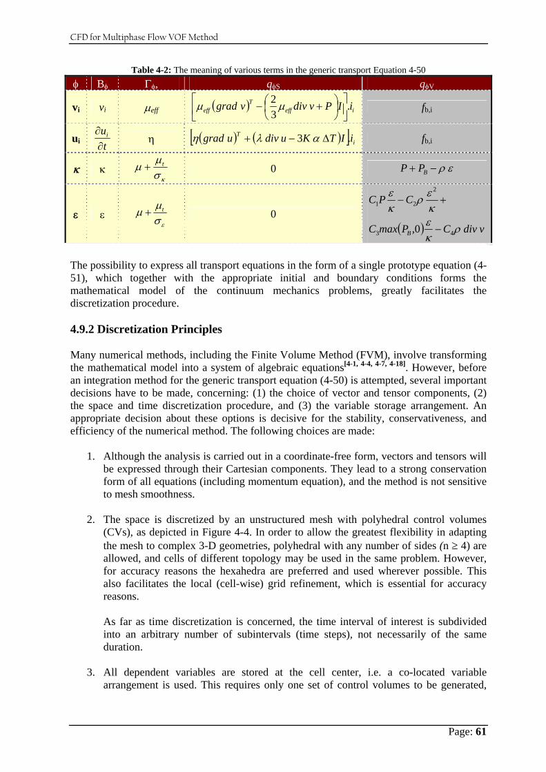
CFD for Multiphase Flow VOF Method

Page: 61

Table 4-2: The meaning of various terms in the generic transport Equation 4-50 φ Bφ Γφ, qφS qφV

vi vi μeff ( ) ieffT

eff iIPv divv grad .32

⎥⎦

⎤⎢⎣

⎡⎟⎠⎞

⎜⎝⎛ +− μμ fb,i

ui tui

∂∂ η ( ) ( )[ ] i

T iIT Ku div u grad .3 Δ−+ αλη fb,i

κ κ κσμμ t+ 0 ερ PP B −+

ε ε εσμμ t+ 0

( ) v div CPmaxC

CPC

B ρκεκερ

κε

43

2

21

0, −

+−

The possibility to express all transport equations in the form of a single prototype equation (4-51), which together with the appropriate initial and boundary conditions forms the mathematical model of the continuum mechanics problems, greatly facilitates the discretization procedure. 4.9.2 Discretization Principles Many numerical methods, including the Finite Volume Method (FVM), involve transforming the mathematical model into a system of algebraic equations[ 4-1, 4-4, 4-7, 4-18]. However, before an integration method for the generic transport equation (4-50) is attempted, several important decisions have to be made, concerning: (1) the choice of vector and tensor components, (2) the space and time discretization procedure, and (3) the variable storage arrangement. An appropriate decision about these options is decisive for the stability, conservativeness, and efficiency of the numerical method. The following choices are made:

1. Although the analysis is carried out in a coordinate-free form, vectors and tensors will be expressed through their Cartesian components. They lead to a strong conservation form of all equations (including momentum equation), and the method is not sensitive to mesh smoothness.

2. The space is discretized by an unstructured mesh with polyhedral control volumes

(CVs), as depicted in Figure 4-4. In order to allow the greatest flexibility in adapting the mesh to complex 3-D geometries, polyhedral with any number of sides (n ≥ 4) are allowed, and cells of different topology may be used in the same problem. However, for accuracy reasons the hexahedra are preferred and used wherever possible. This also facilitates the local (cell-wise) grid refinement, which is essential for accuracy reasons. As far as time discretization is concerned, the time interval of interest is subdivided into an arbitrary number of subintervals (time steps), not necessarily of the same duration.

3. All dependent variables are stored at the cell center, i.e. a co-located variable arrangement is used. This requires only one set of control volumes to be generated,

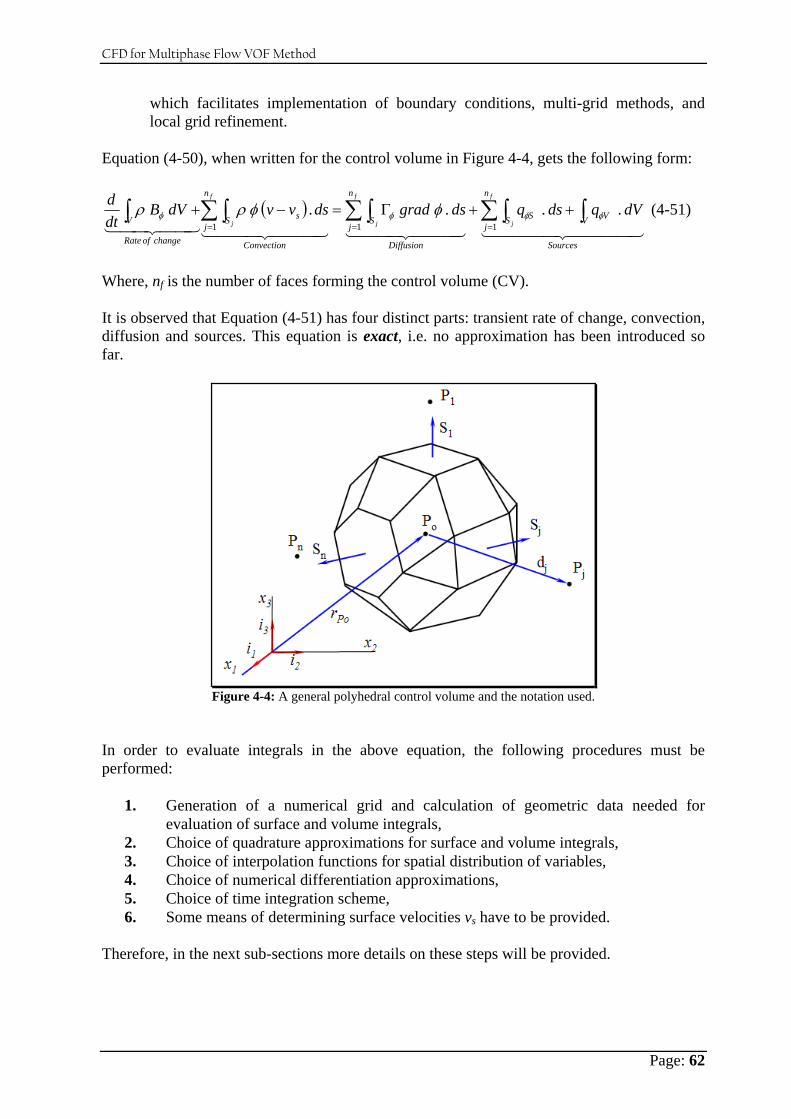
CFD for Multiphase Flow VOF Method

Page: 62

which facilitates implementation of boundary conditions, multi-grid methods, and local grid refinement.

Equation (4-50), when written for the control volume in Figure 4-4, gets the following form:

( )4444 34444 21444 3444 21444 3444 2144 344 21

Sources

V V

n

jS S

Diffusion

n

jS

Convection

n

jS s

change of Rate

VdV qds qds grad ds . vv dV B

dtd f

j

f

j

f

j∫∑∫∑∫∑∫∫ ++Γ=−+

===

...111

φφφφ φφρρ (4-51)

Where, nf is the number of faces forming the control volume (CV). It is observed that Equation (4-51) has four distinct parts: transient rate of change, convection, diffusion and sources. This equation is exact, i.e. no approximation has been introduced so far.

Figure 4-4: A general polyhedral control volume and the notation used.

In order to evaluate integrals in the above equation, the following procedures must be performed:

1. Generation of a numerical grid and calculation of geometric data needed for evaluation of surface and volume integrals,

2. Choice of quadrature approximations for surface and volume integrals, 3. Choice of interpolation functions for spatial distribution of variables, 4. Choice of numerical differentiation approximations, 5. Choice of time integration scheme, 6. Some means of determining surface velocities vs have to be provided.

Therefore, in the next sub-sections more details on these steps will be provided.

CFD for Multiphase Flow VOF Method

Page: 63

4.9.2.1 Numerical Grid The solution domain is subdivided into a finite number of control volumes (CVs) by a numerical grid. The CVs are defined by their vertices, which are joined by straight edges, since the curvature plays no role in the present discretization method. The edges define CV faces, which form a closed CV surface (as shown in Figure 4-4). Numerical evaluation of integrals in Equation 4-51 requires that the coordinates of cell and face centres, surface vector and cell volume be known. This information is provided by the Fluent–VOF pre-processor (Gambit) and stored on a file prior to calculation. Surface vector Since the edges of the CV are straight lines, the projections of the faces onto Cartesian coordinate surfaces are independent of the actual shape of the surface. They represent the Cartesian components of the surface vector, which are calculated by subdividing the cell face into triangles whose surface vectors are easily computed:

( ) ( )[ ]∑=

− −×−=vjn

iiij rrrrS

31112

1 (4-52)

Where v

jn is the number of vertices in cell-face j, and ri is the position vector of the vertex i.

Note that there are vjn -2 triangles. The choice of the common vertex (rl) is not important.

Cell Volume The volume of an arbitrary CV can easily be calculated using Gauss’ theorem as follows:

∑∫ ∫=

=⇒=fn

jjjPoV S

S. rV ds r. dVr div13

1 (4-53)

Where: rj stands for the position vector of the cell-face center j and Sj is the cell-face surface vector. The surface integral is approximated using midpoint rule. In order to avoid overlapping of CVs, the cell-face center and its surface vector have to be uniquely defined. Computational and Boundary nodes Computational nodes at which the variable values are to be calculated are placed at the center of each CV, while boundary nodes are placed at the centers of boundary faces.

4.9.2.2 Calculation of Integrals The surface and volume integrals in Equation 4-51 have to be evaluated using some quadrature approximations. Two levels of approximation are involved: (1) the integral is expressed as a function of the integrand value at one or more locations within the integration domain and (2) these values have to be expressed through the values at computational points (CV centres) in order to obtain an algebraic equation system.

CFD for Multiphase Flow VOF Method

Page: 64

The simplest integral approximation of second order is the midpoint rule and it is used in VOF calculations. The integral is approximated by the product of the integrand at the center of the integration domain and the surface or volume of the domain:

∫ ∫ ≈≈jS V PoPojj V f dV f S. ds ,f.f (4-54)

Where: f and f are arbitrary vector and scalar, respectively.

4.9.2.3 Spatial Variation Variable values and fluid properties are available at the computational nodes, which lie at CV centres[ 4-6]. However, we often need these quantities at locations other than cell centres; to achieve this, interpolation has to be used. Any kind of shape functions could be used; here the simplest second-order approximation, namely linear distribution, is chosen: ( ) ( ) ( )PoPoPo r r gradr −Ψ+Ψ= .ψ (4-55)

Where: ψ stands for the dependent variable φ, physical properties of continuum, or gradient of φj; rpo is the position vector of CV center Po. Cell-face values In order to calculate surface integrals, variable values at cell-face centers are required. Since the Equation 4-55 could lead to a different value rat the cell-face center when applied in CVs on either side of the face, a unique symmetric expression is used when cell-face values are calculated:

( ) ( ) ( ) ( ) ( )[ ]PjjPjPojPopjpoj rr gradrr grad −Ψ+−Ψ+Ψ+Ψ=Ψ ..21

21 (4-56)

Where: rj is the position vector of the cell-face center and Pj denotes the center of the neighbour CV (as displayed in Figure 4-4). The first term on the right hand side (RHS) gives the value at the location midway between cell centers on a straight line connecting Po and Pj. The second term provides correction which takes into account that the cell-face center may not lie on the line connecting cell centers and/or not lie at the midpoint. Gradient calculation In addition to variable values, we also need variable gradients at both cell-face centers and CV centers. In VOF, two methods of calculating gradients are provided: (1) the Gauss theorem, and (2) the least square method. Gauss Theorem: A simple and efficient way of calculating gradients at CV centers to within second-order accuracy is based on the Gauss' divergence theorem and the midpoint-rule integral approximation:

CFD for Multiphase Flow VOF Method

Page: 65

( ) ∑∫∫=

Ψ≈Ψ⇒Ψ=Ψfn

jjj

PoPoSV

SV

grad ds dV grad1

1 (4-57)

Where:

ψj is the value of ψ at the cell-face center j.

4.9.2.4 Integration in Time Equation 4-51 can be rearranged into the following form:

( )φFdt

d=

Ψ (4-58)

Where:

( ) ( )tr VB dV B V PoPo

,and φφρρψ φφ =≈= ∫ (4-58a)

The left hand side (LHS) of Equation 4-58 can be integrated from tm-1 to tm =tm-1 + δtm exactly; the RHS requires an approximation of the mean value of F over the interval δtm. Euler implicit scheme The Euler implicit method uses the current value of F, i.e. the quantity ψ at time tm is calculated as:

mmmm tF δ+Ψ=Ψ −1 (4-59)

Where:

Fm = F(φm), and φm = φ (r, tm). This is a first-order fully-implicit approximation. The convective, diffusive, and source terms are evaluated at the new time level.

4.10 Algebraic Equation Systems Derivation 4.10.1 Convective Fluxes: High-Resolution Interface Capturing Scheme The free-surface capturing method described as mentioned before is based on a convective transport of a scalar quantity which indicates the presence of one of fluids involved in the free-surface flow. The interface is in reality sharp and it should be such in the numerical simulation as well. The use of upwind scheme causes very strong smearing of the interface. The central difference (CD) preserves the sharpness of the interface but at the same time introduces non-physical oscillations around the interface and produces values of the volume fraction which are beyond physically meaningful bounds of 0 and 1. The high-resolution interface capturing scheme (HRIC) is designed to overcome these problems and to model accurately the

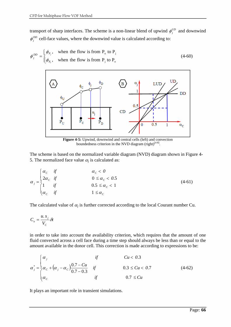
CFD for Multiphase Flow VOF Method

Page: 66

transport of sharp interfaces. The scheme is a non-linear blend of upwind UDjφ and downwind

DDjφ cell-face values, where the downwind value is calculated according to:

⎪⎩

⎪⎨⎧

=oj

jo

P to Pfrom isflow thewhen,

P to Pfrom isflow thewhen,

o

j

P

PDDj φ

φφ (4-60)

Figure 4-5: Upwind, downwind and central cells (left) and convection

boundedness criterion in the NVD diagram (right)[ 4-8]. The scheme is based on the normalized variable diagram (NVD) diagram shown in Figure 4-5. The normalized face value αj is calculated as:

⎪⎪⎩

⎪⎪⎨

⎧

≤<≤

<≤<

=

if if

0 if 0 if

CC

C

CC

CC

j

ααα

αααα

α

115.015.02

(4-61)

The calculated value of αj is further corrected according to the local Courant number Cu.

tV su

CC

ju δ

.=

in order to take into account the availability criterion, which requires that the amount of one fluid convected across a cell face during a time step should always be less than or equal to the amount available in the donor cell. This correction is made according to expressions to be:

( )⎪⎪⎩

⎪⎪⎨

⎧

≤

<≤−−

−+

<

=

Cu if

0 Cu if Cu0 Cu if

C

CjC

j

j

7.0

7.3.03.07.0

7.03.

*

α

ααα

α

α (4-62)

It plays an important role in transient simulations.

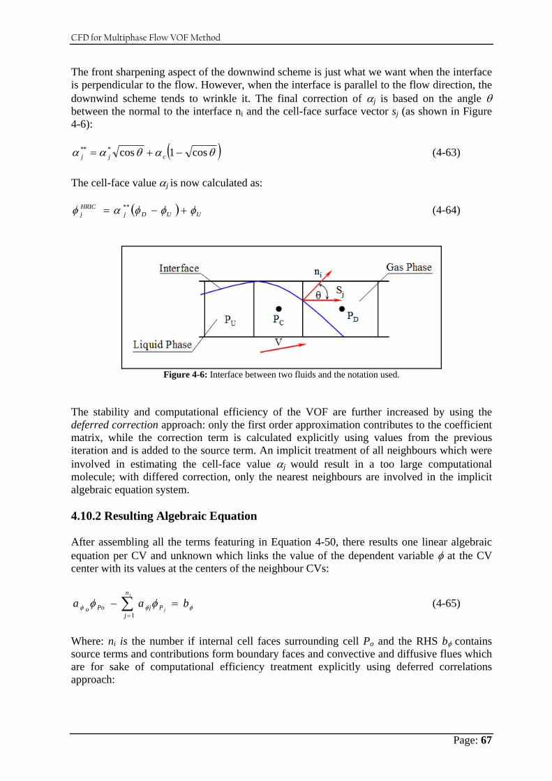
CFD for Multiphase Flow VOF Method

Page: 67

The front sharpening aspect of the downwind scheme is just what we want when the interface is perpendicular to the flow. However, when the interface is parallel to the flow direction, the downwind scheme tends to wrinkle it. The final correction of αj is based on the angle θ between the normal to the interface ni and the cell-face surface vector sj (as shown in Figure 4-6):

( )θαθαα cjj cos1cos*** −+= (4-63) The cell-face value αj is now calculated as:

( ) UUDjHRICj φφφαφ +−= ** (4-64)

Figure 4-6: Interface between two fluids and the notation used.

The stability and computational efficiency of the VOF are further increased by using the deferred correction approach: only the first order approximation contributes to the coefficient matrix, while the correction term is calculated explicitly using values from the previous iteration and is added to the source term. An implicit treatment of all neighbours which were involved in estimating the cell-face value αj would result in a too large computational molecule; with differed correction, only the nearest neighbours are involved in the implicit algebraic equation system. 4.10.2 Resulting Algebraic Equation After assembling all the terms featuring in Equation 4-50, there results one linear algebraic equation per CV and unknown which links the value of the dependent variable φ at the CV center with its values at the centers of the neighbour CVs:

φφφ φφ baai

j

n

jPjPoo

=− ∑=1

(4-65)

Where: ni is the number if internal cell faces surrounding cell Po and the RHS bφ contains source terms and contributions form boundary faces and convective and diffusive flues which are for sake of computational efficiency treatment explicitly using deferred correlations approach:

CFD for Multiphase Flow VOF Method

Page: 68

( )

( )

( ) ( ) ( ) ( ) ( ) ( )( )

tB

n

BBV

jpPPjPjjPoPojj

n

j

jj

jjjjj

n

j

t

n

j

jjj

jj

qaqq

m grad rr grad rrm

S d S S

d grad S gradb

aaa

m S d S S

a

B

S

oj

f

f

j

f

jj

jj

φφφφ

φ

φφ

φφφ

φφ

φ

φφφφγ

φφ

+++

+−+−+−

−⎟⎟⎠

⎞⎜⎜⎝

⎛−Γ=

+=

−Γ=

∑

∑

∑

∑

=

=

=

=

1

1

1

1

sgn..2

.

...

0,min..

&&

&

(4-66)

Where: nB=nf-ni is the number of boundary faces surrounding cell Po and aφt and qφt are calculated for Euler implicit scheme as follows:

( )m

mPo

t tVaδρ

φ = (4-67)

( )

m

mPo

t tVqδρ

φ = (4-68)

4.10.3 Calculation of Pressure Based on the previous procedures, the pressure, featuring in the source term of the fluid momentum equation, has remained unknown, while at the same time no use has been made of the continuity equation. The problem lies in the fact that the pressure does not feature explicitly in the continuity equation which consequently can not be considered as 'an equation for pressure' and the continuity equation for incompressible flows acts just as an additional constraint on the velocity field. This constraint can be satisfied only by adjusting the pressure field. However, pressure is not a conserved property and does not have its governing transport equation, so it is not obvious how this adjustment of pressure is to be performed. At the same time, the pressure source term in the momentum equation is calculated using second-order space-cantered scheme. As mentioned earlier, such a scheme can produce a correct pressure-gradient field, even if the underlying pressure field is contaminated by unphysical oscillations. In order to calculate the pressure field and to couple it properly to the velocity field, a pressure-correction method of SIMPLE-type is used[ 4-10]. Cell-face Velocity and density The simple and yet efficient way of getting around of the aforementioned problem of pressure oscillations is to calculate the fluid velocity at a cell face in the following manner:

jj

jj

j

j

j

PoPj

vo

Pojj Sd

Sd

dd P grad

dPP

aVvv

..*

⎪⎭

⎪⎬⎫

⎪⎩

⎪⎨⎧

−−

⎟⎟⎠

⎞⎜⎜⎝

⎛−= (4-69)

Where:

CFD for Multiphase Flow VOF Method

Page: 69

vj is the spatially interpolating velocity. The density used in the calculation of the mass is computed as follows:

( )UDj

CDj

UDjj ρργρρ ρ −+=* (4-70)

Where blending of the second-order accurate CD value with some small amount (typically γρ = 0.90 to 0.95) of UD value is sometimes necessary for stability reasons. Predictor stage; pressure-correction equation The so-called predictor stage values of v, P and ρ which satisfy the momentum equation, do not necessarily satisfy the continuity Equation 4-1, which can be written for Euler implicit scheme in the following form: ( ) ( ) 0

1

1

=+− ∑

=

− fn

jj

m

mPoPo m

tVV

&δ

ρρ (4-71)

By employing now the co-located version of the SIMPLE algorithm for compressible flow, a new equation for pressure correction P′ is obtained from the requirement that corrected mass fluxes satisfy the continuity equation:

P

n

jPjjpPoop bPaPa

f

′=

′′ =′−′ ∑1

(4-72)

With coefficients:

( ) ( )

( ) ( ){ PVPVmb

Pt

Vaa

P Sv Sv

Sd SS

aVa

mPoPo

n

jjP

Pm

Pn

jPP

PPj

jjjjjj

jj

vo

PojP

f

o

of

jo

j

1

1

1

***

ˆ

.210,.min1

.

.

−

=′

=′′

′

−−−=

⎪⎩

⎪⎨⎧

⎟⎠⎞

⎜⎝⎛∂∂

+=

⎟⎠⎞

⎜⎝⎛∂∂

⎥⎦⎤

⎢⎣⎡ +−−⎟⎟

⎠

⎞⎜⎜⎝

⎛=

∑

∑

&

ρδ

βργγρ ρρ

(4-73)

where all variables have their predictor stage values and avo is the corresponding momentum equation central coefficient, jPa ′ˆ is the conjugate of jPa ′ , i.e. the coefficient related to the cell-face j when Po and Pj exchange their roles (when the pressure correction equation for cell Pj is

constructed), and P∂∂ρ is calculated from an equation of state.

Boundary conditions The boundary conditions for the pressure-correction equation depend on the boundary conditions for the momentum equations. On those portions of the boundary where the velocity is prescribed, its correction is zero which implies a zero-gradient boundary condition on the pressure correction. If the pressure is prescribed at the boundary, than its correction is zero,

CFD for Multiphase Flow VOF Method

Page: 70

leading to a Dirichlet boundary condition for the pressure correction. In the case of incompressible flows, the mass flow rate is usually prescribed so the pressure-correction equation has Neumann boundary conditions on all boundaries and the sum of sources is equal to zero; the equation then has an infinite number of solutions, all deferring by a constant. This causes no problem since for such flows the absolute pressure level is unimportant - only the gradient is important. The pressure is fixed to a reference value (typical zero) at one cell center and only differences relative to this node are calculated. In the case of compressible flows, the absolute pressure is important; the pressure is then usually (directly or indirectly) specified on at least one portion of the boundary. It is worth mentioning that in the case of constant density or low speed variable density flows (Mach number less than 0.3) the density corrections can be neglected, which leads to a pressure correction equation with a symmetric coefficient matrix, which in some situations becomes singular. However, if the problem is well posed, the resulting set of linear algebraic equations is undetermined, which practically means that the pressure correction, and consequently the pressure level is undetermined. This, however, has no consequences on the solution, since only pressure gradients, and not the pressure itself, feature in fluid momentum equation.

4.11 Nomenclature

CV Control volume Cv Specific heat at constant volume D Rate of strain tensor

Di,t,,μt Turbulent diffusivity coefficients E Sum of the specific internal or thermal energy fb Body force per unit volume

Gr Grashof Number K Thermal conductivity or Mean curvature of the free-surface L Length nf Number of faces forming the control volume (CV). P Pressure qh Heat flux vector R Universal gas constant

Ra Rayleigh Re Reynolds number

s Outward pointing surface vector Sh Heat source or sink T Cauchy stress tensor V Continuum volume

v, vs Velocity and surface velocity vj Spatially interpolating velocity ρ Density μ Dynamic Viscosity τ Time interval κ Turbulent kinetic energy ε Turbulent dissipation σ Surface tension β Volumetric thermal expansion coefficient

CFD for Multiphase Flow VOF Method

Page: 71

δfs Small finite thickness ρref Density at a reference temperature Tref. κt Conductivity ΔT Characteristic temperature difference

4.12 References

4-1. Comet User Manual (n. d.), ICCM Institute of Computational Continuum Mechanics GmbH, Hamburg, Germany, available at: www.iccm.de.

4-2. Patankar, S. V.: Numerical Heat Transfer and Fluid Flow, Series in Computational Methods in Mechanics and Thermal Sciences, Hemisphere Publishing Corporation, McGraw Hill, New York, USA, ISBN 0-89116-522-3, 1980.

4-3. Ashgriz, N. and Mostaghimi, J.: Computational Fluid Dynamics, Chapter 24 in Fluid Flow Handbook, McGrew Hill Publishing, ISBN 0-07-136372-6, 2002.

4-4. Chung, T. J.: Computational Fluid Dynamics, Cambridge University Press, ISBN 0 521 59416 2, 2002.

4-5. Anderson, J.D., Jr.: Computational Fluid Dynamics: The Basics with Applications, McGraw-Hill International Edition, McGraw-Hill, Inc., 1995.

4-6. Blazek, J.: Computational Fluid Dynamics: Principles and Applications, Elsevier Science, 2001.

4-7. Fletcher, C. A. J.: Computational Techniques for Fluid Dynamics: Vol. 2 Specific Techniques for Different Flow Categories, Berlin, Springer – Verlag, 1991.

4-8. Tannehill, J. C., Anderson, D. A. and Pletcher, R. H.: Computational Fluid Mechanics and Heat Transfer, 2nd Ed., Taylor & Francis, ISBN 1 56032 045X, 1997.

4-9. Bates, P. D., Lane, S. N. and Ferguson, R. I.: Computational Fluid Dynamics: Applications in Environmental Hydraulics, Chapter 1: CFD Modelling for Environmental Hydraulics, John Wiley & Sons, Ltd, ISBN 9780470843598, 2005.

4-10. Hoffmann, K. A. and Chiang, S. T.: Computational Fluid Dynamics for Engineers, Vol. III, 4th Ed., Engineering Education Systems, ISBN 0962373133, Wichita, USA, 2000.

4-11. Fluent Inc., User’s Guide for Fluent 6.3, http://www.fluent.com, Lebanon, NH, 2006.

4-12. Hirt, C. W. and Nichols, B. D.: “Volume of Fluid (VOF) Method for the Dynamics of Free Boundaries,” Journal of Computational Physics, Vol. 39, No. 1, Pages 201-225, Jan. 1981.

4-13. Wilcox, D. C.: Turbulence Modeling for CFD, ISBN 1-928729-10-X, 2nd 2 Ed., DCW Industries, La Canada, California, 2000.

4-14. Drikakis, D. and Geurto, B. J.: Turbulent Flow Computation, Kluwer Academic Pub., 2002.

4-15. Pope, S. B.: Turbulent Flow, Cambridge University Press, Cambridge, 2000. 4-16. Cebeci, T, Shao, J. P, Kafyeke, F. and Laurendeau, E.: CFD for Engineers, ISBN 3-

540-24451-4, Berlin, Springer – Verlag, 2005. 4-17. Ferziger, J. H. and Peric, M.: Computational Methods for Fluid Dynamics, 3rd ed.,

Springer-Verlag, ISBN 3540420746, 2001. 4-18. Peyret, R.: Handbook of Computational Fluid Mechanics, Academic Press, 1996.

Numerical Simulation of Two Phase Flow

Page: 72

CHAPTER V

Numerical Simulation of Two Phase Flow

Phenomena in Horizontal and Inclined Pipes

Stratified & Slug Flow Characterizations

5.1 Introduction Two-phase flow in natural crude oil transmission pipelines is common. Accurate knowledge of the pressure profile and liquid distribution as predicted with an appropriate model is necessary for optimal design and sitting of downstream facilities. For the gas-gathering pipeline system, it is important to determine the size of each line from the point of pressure loss and prevention of backflow from a well to another. The calculations required for sizing the pipelines include phase behaviour, pressure drop, temperature profiles, liquid volumes, flow pattern prediction, liquid flow rates and minimum gas velocity [ 5-1, 5-2]. The simultaneous flow of liquid and gas in a pipeline can result in several different flow patterns. These flow patterns are dependent on the flow rates of liquid and gas. Flow patterns are also dependent on the elevation profile of the pipeline. Generally, there are several methods available to assess the flow behaviour in multi-phase pipe flows[ 5-3, 5-4, 5-5, 5-6, 5-7]. All flow regimes however, can be grouped into dispersed flow, separated flow and intermittent flow or a combination of these as shown in the Figure 2-2. The first set of simulation runs was performed to compute flow patterns in horizontal and the second set predicts the flow regimes in inclined pipelines (+5°). Each set consists of several simulation experiments covering a wide range of flow rates of gas and liquid. The results of the first set were verified against experimental work done recently and two different flow maps have been drawn, one for horizontal flow and one for inclined pipe flows. Stratified flow conditions as well as slug flow characteristics have been calculated and new relationships between the superficial liquid velocity, pressure drop and liquid hold up have been derived. The ultimate aim of this work was to gain a deeper understanding of multiphase flow phenomena in pipelines and to develop guidelines to improve the design of pipelines and separation facilities. Based on this simulation experiences a practical application was performed in a large field scale pipeline belonging to OMV-Austria presented in the next chapter.

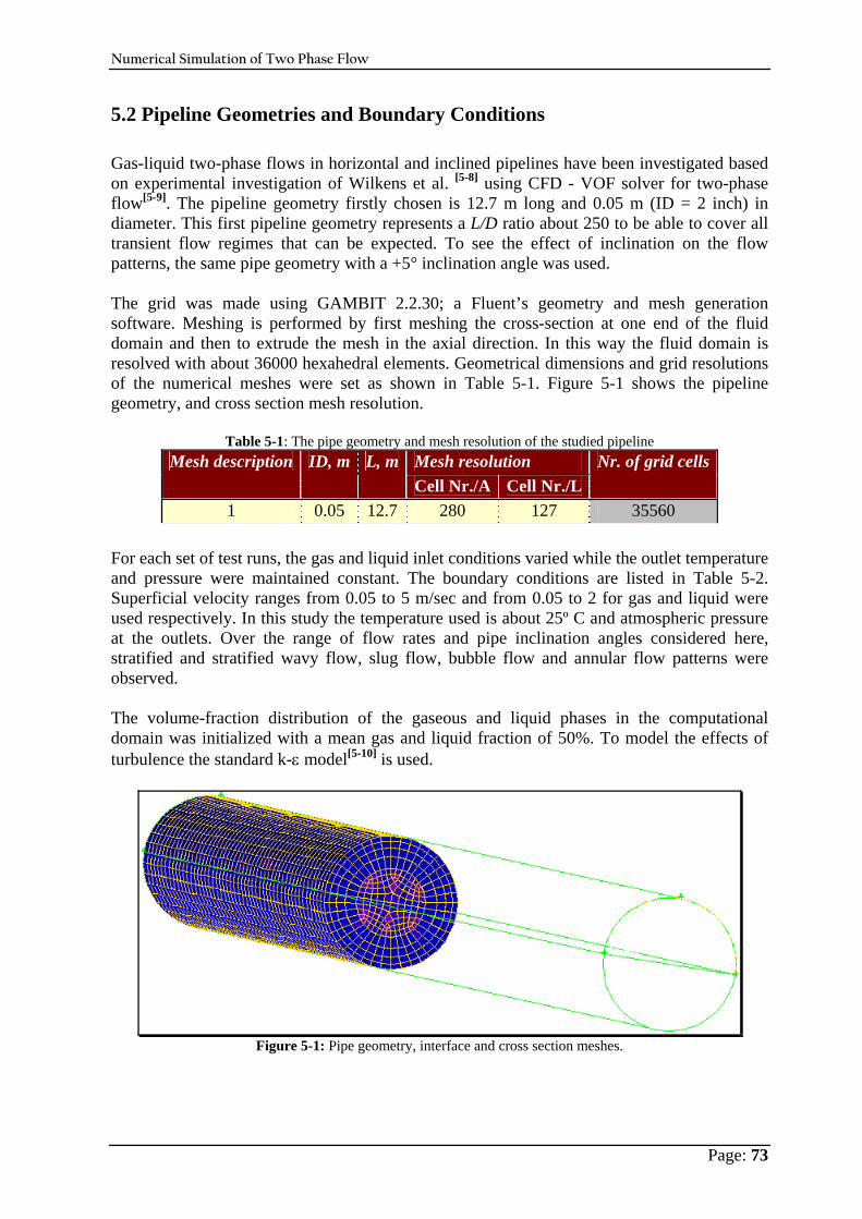
Numerical Simulation of Two Phase Flow

Page: 73

5.2 Pipeline Geometries and Boundary Conditions Gas-liquid two-phase flows in horizontal and inclined pipelines have been investigated based on experimental investigation of Wilkens et al. [ 5-8] using CFD - VOF solver for two-phase flow[ 5-9]. The pipeline geometry firstly chosen is 12.7 m long and 0.05 m (ID = 2 inch) in diameter. This first pipeline geometry represents a L/D ratio about 250 to be able to cover all transient flow regimes that can be expected. To see the effect of inclination on the flow patterns, the same pipe geometry with a +5° inclination angle was used. The grid was made using GAMBIT 2.2.30; a Fluent’s geometry and mesh generation software. Meshing is performed by first meshing the cross-section at one end of the fluid domain and then to extrude the mesh in the axial direction. In this way the fluid domain is resolved with about 36000 hexahedral elements. Geometrical dimensions and grid resolutions of the numerical meshes were set as shown in Table 5-1. Figure 5-1 shows the pipeline geometry, and cross section mesh resolution.

Table 5-1: The pipe geometry and mesh resolution of the studied pipeline Mesh resolution Mesh description ID, m L, mCell Nr./A Cell Nr./L

Nr. of grid cells

1 0.05 12.7 280 127 35560 For each set of test runs, the gas and liquid inlet conditions varied while the outlet temperature and pressure were maintained constant. The boundary conditions are listed in Table 5-2. Superficial velocity ranges from 0.05 to 5 m/sec and from 0.05 to 2 for gas and liquid were used respectively. In this study the temperature used is about 25º C and atmospheric pressure at the outlets. Over the range of flow rates and pipe inclination angles considered here, stratified and stratified wavy flow, slug flow, bubble flow and annular flow patterns were observed. The volume-fraction distribution of the gaseous and liquid phases in the computational domain was initialized with a mean gas and liquid fraction of 50%. To model the effects of turbulence the standard k-ε model[ 5-10] is used.

Figure 5-1: Pipe geometry, interface and cross section meshes.

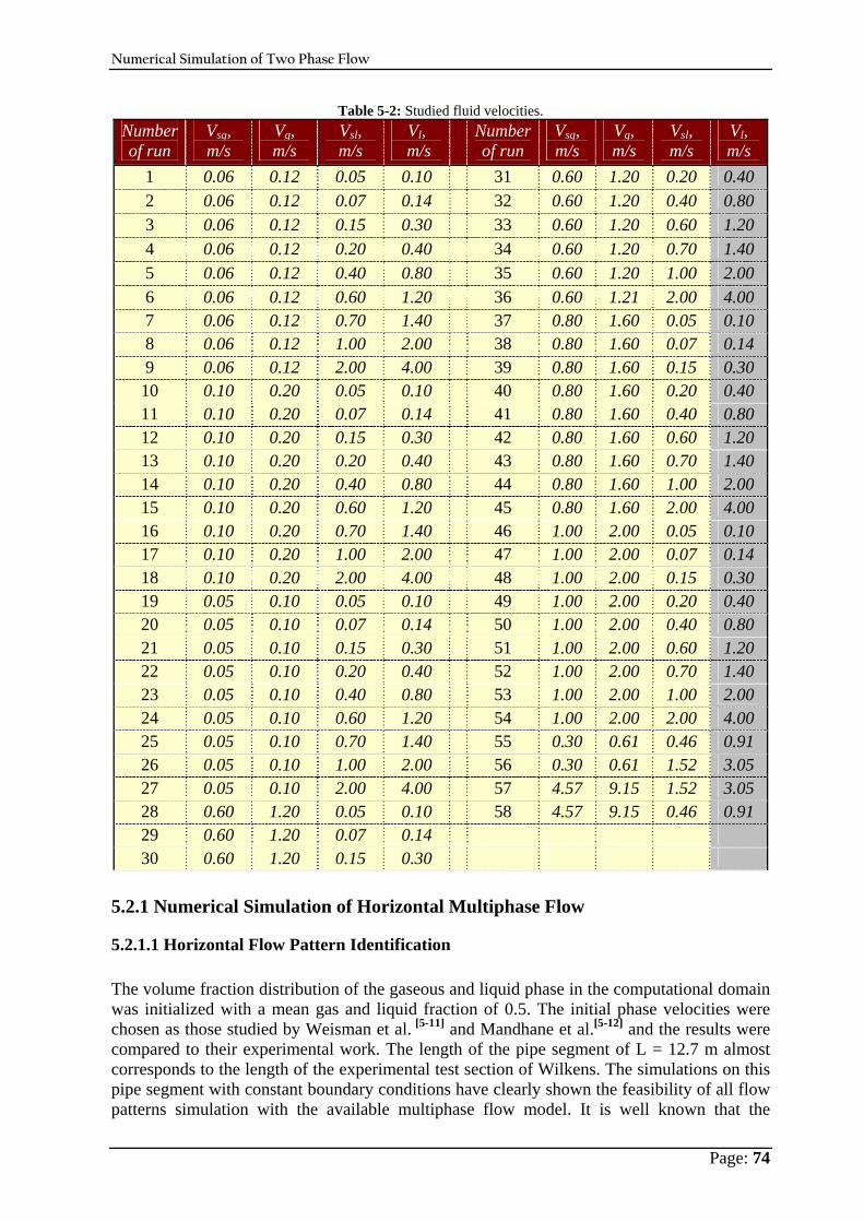
Numerical Simulation of Two Phase Flow

Page: 74

Table 5-2: Studied fluid velocities. Number of run

Vsg, m/s

Vg, m/s

Vsl, m/s

Vl, m/s

Number of run

Vsg, m/s

Vg, m/s

Vsl, m/s

Vl, m/s

1 0.06 0.12 0.05 0.10 31 0.60 1.20 0.20 0.40 2 0.06 0.12 0.07 0.14 32 0.60 1.20 0.40 0.80 3 0.06 0.12 0.15 0.30 33 0.60 1.20 0.60 1.20 4 0.06 0.12 0.20 0.40 34 0.60 1.20 0.70 1.40 5 0.06 0.12 0.40 0.80 35 0.60 1.20 1.00 2.00 6 0.06 0.12 0.60 1.20 36 0.60 1.21 2.00 4.00 7 0.06 0.12 0.70 1.40 37 0.80 1.60 0.05 0.10 8 0.06 0.12 1.00 2.00 38 0.80 1.60 0.07 0.14 9 0.06 0.12 2.00 4.00 39 0.80 1.60 0.15 0.30 10 0.10 0.20 0.05 0.10 40 0.80 1.60 0.20 0.40 11 0.10 0.20 0.07 0.14 41 0.80 1.60 0.40 0.80 12 0.10 0.20 0.15 0.30 42 0.80 1.60 0.60 1.20 13 0.10 0.20 0.20 0.40 43 0.80 1.60 0.70 1.40 14 0.10 0.20 0.40 0.80 44 0.80 1.60 1.00 2.00 15 0.10 0.20 0.60 1.20 45 0.80 1.60 2.00 4.00 16 0.10 0.20 0.70 1.40 46 1.00 2.00 0.05 0.10 17 0.10 0.20 1.00 2.00 47 1.00 2.00 0.07 0.14 18 0.10 0.20 2.00 4.00 48 1.00 2.00 0.15 0.30 19 0.05 0.10 0.05 0.10 49 1.00 2.00 0.20 0.40 20 0.05 0.10 0.07 0.14 50 1.00 2.00 0.40 0.80 21 0.05 0.10 0.15 0.30 51 1.00 2.00 0.60 1.20 22 0.05 0.10 0.20 0.40 52 1.00 2.00 0.70 1.40 23 0.05 0.10 0.40 0.80 53 1.00 2.00 1.00 2.00 24 0.05 0.10 0.60 1.20 54 1.00 2.00 2.00 4.00 25 0.05 0.10 0.70 1.40 55 0.30 0.61 0.46 0.91 26 0.05 0.10 1.00 2.00 56 0.30 0.61 1.52 3.05 27 0.05 0.10 2.00 4.00 57 4.57 9.15 1.52 3.05 28 0.60 1.20 0.05 0.10 58 4.57 9.15 0.46 0.91 29 0.60 1.20 0.07 0.14 30 0.60 1.20 0.15 0.30

5.2.1 Numerical Simulation of Horizontal Multiphase Flow

5.2.1.1 Horizontal Flow Pattern Identification The volume fraction distribution of the gaseous and liquid phase in the computational domain was initialized with a mean gas and liquid fraction of 0.5. The initial phase velocities were chosen as those studied by Weisman et al. [ 5-11] and Mandhane et al.[ 5-12] and the results were compared to their experimental work. The length of the pipe segment of L = 12.7 m almost corresponds to the length of the experimental test section of Wilkens. The simulations on this pipe segment with constant boundary conditions have clearly shown the feasibility of all flow patterns simulation with the available multiphase flow model. It is well known that the

Numerical Simulation of Two Phase Flow

Page: 75

interface between the phases normally does not touch the upper internal surface of the pipeline for stratified flow. But the interface hits the upper surface of the pipe in the case of slug flow. This is demonstrated by the liquid holdup as shown in Figure 5-2 for two different simulation runs. Figure 5-2-a displays the behaviour of liquid holdup for a stratified flow at two different positions in the pipeline while Figure 5-2-b depicts the holdup variations for a slug flow regime at three different locations in the pipeline versus time. The liquid holdup in the slug increases sharply from the front of the slug to a maximum in the body. Based on visual observations and the extensive data sets that were collected each flow regime was identified (Figure 5-3), and each set of runs was categorized to represent a certain region in the flow pattern diagram. We end up with all of these categorized sets plotted on two of the published maps of Mandhane et al. [ 5-12] and Weisman et al. [ 5-9]. A good agreement between the two flow maps was observed except for minor regions as shown in Figure 5-4.

Vsg = 0.06 m/s & Vsl =  0.05 m/s

0.00

0.10

0.20

0.30

0.40

0.50

0.60

0.70

0.80

0.90

1.00

0 10 20 30 40 50Time, sec

Liquid Holdup, fracion

Liquid Holdup at 3m

Liquid Holdup at 6m

(5-2-a)

Vsg = 0.8 m/s & Vsl = 0.7 m/s

0.0

0.1

0.2

0.3

0.4

0.5

0.6

0.7

0.8

0.9

1.0

0 2 4 6 8 10Time, sec

Liquid Holdup, fraction

Liquid Holdup at 3mLiquid Holdup at 6mLiquid Holdup at 9m

(5-2-b) Figure 5-2: CFD potential for different flow regime modelling.

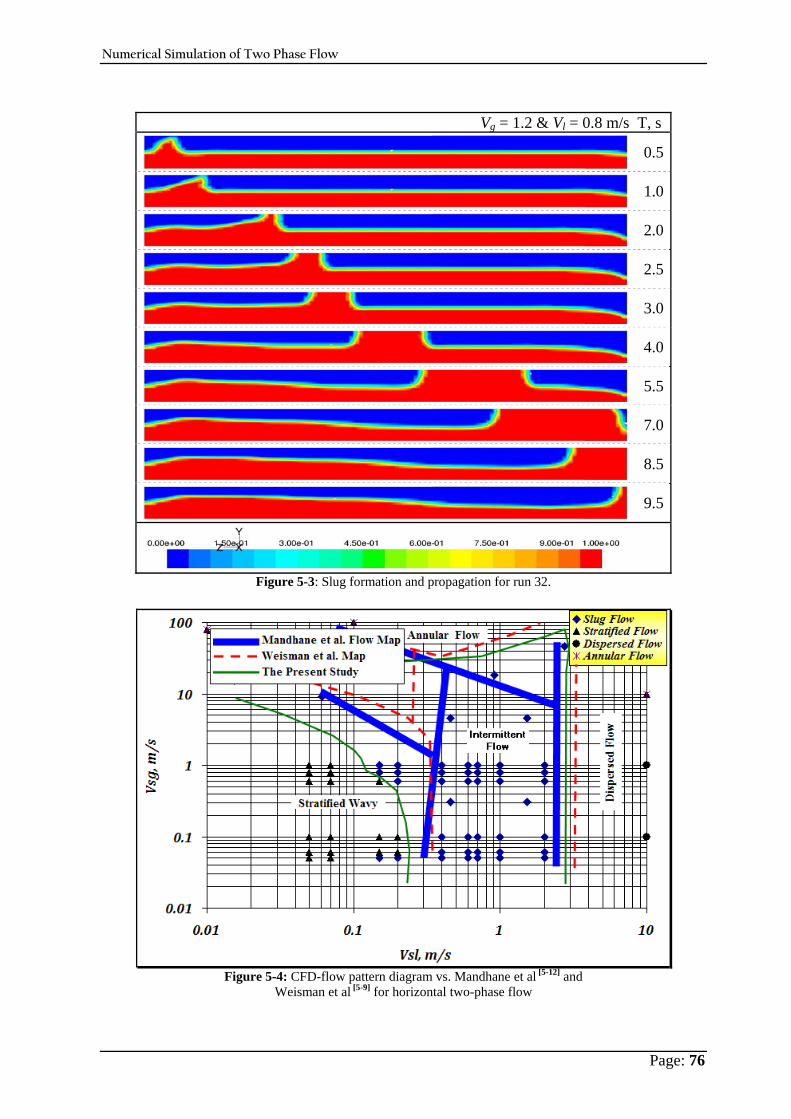
Numerical Simulation of Two Phase Flow

Page: 76

Vg = 1.2 & Vl = 0.8 m/s T, s

0.5

1.0

2.0

2.5

3.0

4.0

5.5

7.0

8.5

9.5

Figure 5-3: Slug formation and propagation for run 32.

Figure 5-4: CFD-flow pattern diagram vs. Mandhane et al [ 5-12] and

Weisman et al [ 5-9] for horizontal two-phase flow

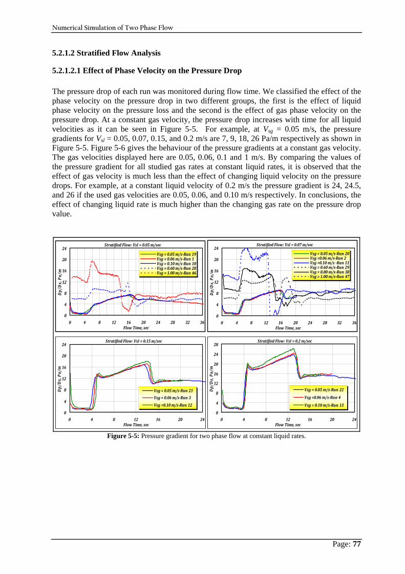
Numerical Simulation of Two Phase Flow

Page: 77

5.2.1.2 Stratified Flow Analysis

5.2.1.2.1 Effect of Phase Velocity on the Pressure Drop The pressure drop of each run was monitored during flow time. We classified the effect of the phase velocity on the pressure drop in two different groups, the first is the effect of liquid phase velocity on the pressure loss and the second is the effect of gas phase velocity on the pressure drop. At a constant gas velocity, the pressure drop increases with time for all liquid velocities as it can be seen in Figure 5-5. For example, at Vsg = 0.05 m/s, the pressure gradients for Vsl = 0.05, 0.07, 0.15, and 0.2 m/s are 7, 9, 18, 26 Pa/m respectively as shown in Figure 5-5. Figure 5-6 gives the behaviour of the pressure gradients at a constant gas velocity. The gas velocities displayed here are 0.05, 0.06, 0.1 and 1 m/s. By comparing the values of the pressure gradient for all studied gas rates at constant liquid rates, it is observed that the effect of gas velocity is much less than the effect of changing liquid velocity on the pressure drops. For example, at a constant liquid velocity of 0.2 m/s the pressure gradient is 24, 24.5, and 26 if the used gas velocities are 0.05, 0.06, and 0.10 m/s respectively. In conclusions, the effect of changing liquid rate is much higher than the changing gas rate on the pressure drop value.

Stratified Flow: Vsl = 0.05 m/sec

0

4

8

12

16

20

24

0 4 8 12 16 20 24 28 32 36Flow Time, sec

Dp/Dx, Pa/m

Vsg = 0.05 m/s­Run 19Vsg = 0.06 m/s­Run 1Vsg = 0.10 m/s­Run 10Vsg = 0.60 m/s­Run 28Vsg = 1.00 m/s­Run 46

Stratified Flow: Vsl = 0.07 m/sec

0

4

8

12

16

20

24

0 4 8 12 16 20 24 28 32 36Flow Time, sec

Dp/Dx, Pa/m

Vsg = 0.05 m/s­Run 20Vsg =0.06 m/s­Run 2Vsg =0.10 m/s ­Run 11Vsg = 0.60 m/s­Run 29Vsg = 0.80 m/s­Run 38Vsg = 1.00 m/s­Run 47

Stratified Flow: Vsl = 0.15 m/sec

0

4

8

12

16

20

24

0 4 8 12 16 20 24Flow Time, sec

Dp/Dx, Pa/m

Vsg = 0.05 m/s­Run 21

Vsg = 0.06 m/s­Run 3

Vsg =0.10 m/s­Run 12

Stratified Flow: Vsl = 0.2 m/sec

0

4

8

12

16

20

24

28

0 4 8 12 16 20 24Flow Time, sec

Dp/Dx, Pa/m

Vsg = 0.05 m/s­Run 22

Vsg =0.06 m/s­Run 4

Vsg = 0.10 m/s­Run 13

Figure 5-5: Pressure gradient for two phase flow at constant liquid rates.

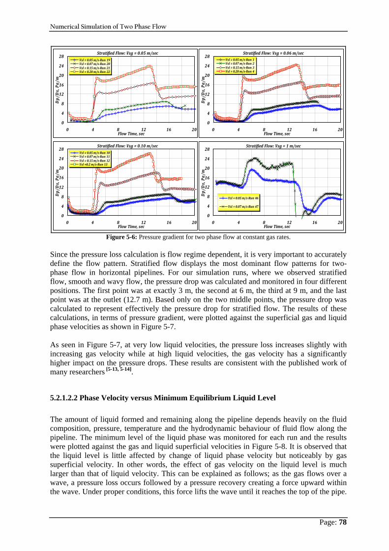
Numerical Simulation of Two Phase Flow

Page: 78

Stratified Flow: Vsg = 0.05 m/sec

0

4

8

12

16

20

24

28

0 4 8 12 16 20Flow Time, sec

Dp/D

x, Pa/m

Vsl = 0.05 m/s­Run 19Vsl = 0.07 m/s­Run 20Vsl = 0.15 m/s­Run 21Vsl = 0.20 m/s­Run 22

Stratified Flow: Vsg = 0.06 m/sec

0

4

8

12

16

20

24

28

0 4 8 12 16 20Flow Time, sec

Dp/D

x, Pa/m

Vsl = 0.05 m/s­Run 1Vsl = 0.07 m/s­Run 2Vsl = 0.15 m/s­Run 3Vsl = 0.20 m/s­Run 4

Stratified Flow: Vsg = 0.10 m/sec

0

4

8

12

16

20

24

28

0 4 8 12 16 20Flow Time, sec

Dp/Dx, Pa/m

Vsl = 0.05 m/s­Run 10Vsl = 0.07 m/s­Run 11Vsl = 0.15 m/s­Run 12Vsl =0.2 m/s­Run 13

Stratified Flow: Vsg = 1 m/sec

0

4

8

12

16

20

24

28

0 4 8 12 16 20Flow Time, sec

Dp/D

x, Pa/m

Vsl = 0.05 m/s­Run 46

Vsl = 0.07 m/s­Run 47

Figure 5-6: Pressure gradient for two phase flow at constant gas rates. Since the pressure loss calculation is flow regime dependent, it is very important to accurately define the flow pattern. Stratified flow displays the most dominant flow patterns for two-phase flow in horizontal pipelines. For our simulation runs, where we observed stratified flow, smooth and wavy flow, the pressure drop was calculated and monitored in four different positions. The first point was at exactly 3 m, the second at 6 m, the third at 9 m, and the last point was at the outlet (12.7 m). Based only on the two middle points, the pressure drop was calculated to represent effectively the pressure drop for stratified flow. The results of these calculations, in terms of pressure gradient, were plotted against the superficial gas and liquid phase velocities as shown in Figure 5-7. As seen in Figure 5-7, at very low liquid velocities, the pressure loss increases slightly with increasing gas velocity while at high liquid velocities, the gas velocity has a significantly higher impact on the pressure drops. These results are consistent with the published work of many researchers [ 5-13, 5-14].

5.2.1.2.2 Phase Velocity versus Minimum Equilibrium Liquid Level The amount of liquid formed and remaining along the pipeline depends heavily on the fluid composition, pressure, temperature and the hydrodynamic behaviour of fluid flow along the pipeline. The minimum level of the liquid phase was monitored for each run and the results were plotted against the gas and liquid superficial velocities in Figure 5-8. It is observed that the liquid level is little affected by change of liquid phase velocity but noticeably by gas superficial velocity. In other words, the effect of gas velocity on the liquid level is much larger than that of liquid velocity. This can be explained as follows; as the gas flows over a wave, a pressure loss occurs followed by a pressure recovery creating a force upward within the wave. Under proper conditions, this force lifts the wave until it reaches the top of the pipe.

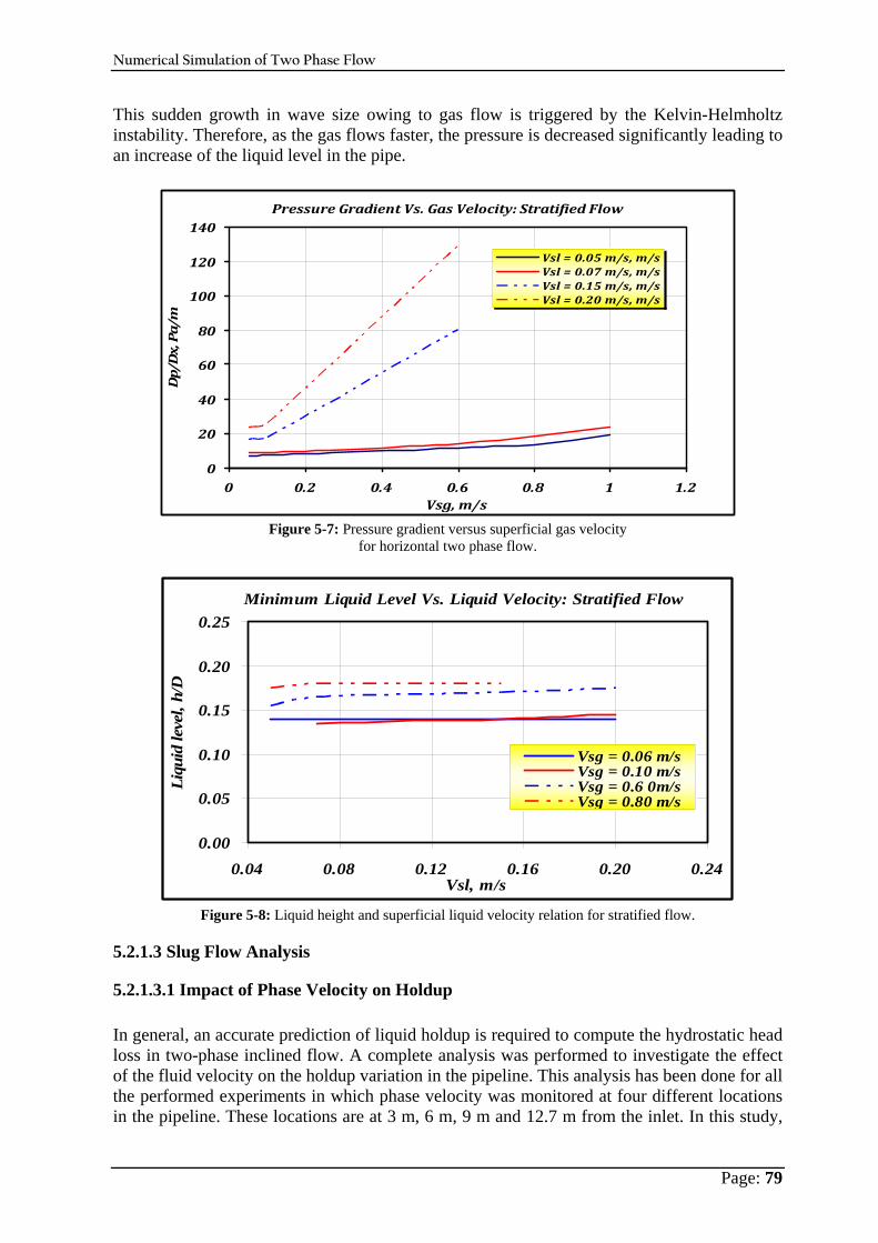
Numerical Simulation of Two Phase Flow

Page: 79

This sudden growth in wave size owing to gas flow is triggered by the Kelvin-Helmholtz instability. Therefore, as the gas flows faster, the pressure is decreased significantly leading to an increase of the liquid level in the pipe.

Pressure Gradient Vs. Gas Velocity: Stratified Flow

0

20

40

60

80

100

120

140

0 0.2 0.4 0.6 0.8 1 1.2Vsg, m/s

Dp/Dx, Pa/m

Vsl = 0.05 m/s, m/sVsl = 0.07 m/s, m/sVsl = 0.15 m/s, m/sVsl = 0.20 m/s, m/s

Figure 5-7: Pressure gradient versus superficial gas velocity

for horizontal two phase flow.

Minimum Liquid Level Vs. Liquid Velocity: Stratified Flow

0.00

0.05

0.10

0.15

0.20

0.25

0.04 0.08 0.12 0.16 0.20 0.24Vsl, m/s

Liqu

id le

vel,

h/D

Vsg = 0.06 m/sVsg = 0.10 m/sVsg = 0.6 0m/sVsg = 0.80 m/s

Figure 5-8: Liquid height and superficial liquid velocity relation for stratified flow.

5.2.1.3 Slug Flow Analysis

5.2.1.3.1 Impact of Phase Velocity on Holdup In general, an accurate prediction of liquid holdup is required to compute the hydrostatic head loss in two-phase inclined flow. A complete analysis was performed to investigate the effect of the fluid velocity on the holdup variation in the pipeline. This analysis has been done for all the performed experiments in which phase velocity was monitored at four different locations in the pipeline. These locations are at 3 m, 6 m, 9 m and 12.7 m from the inlet. In this study,

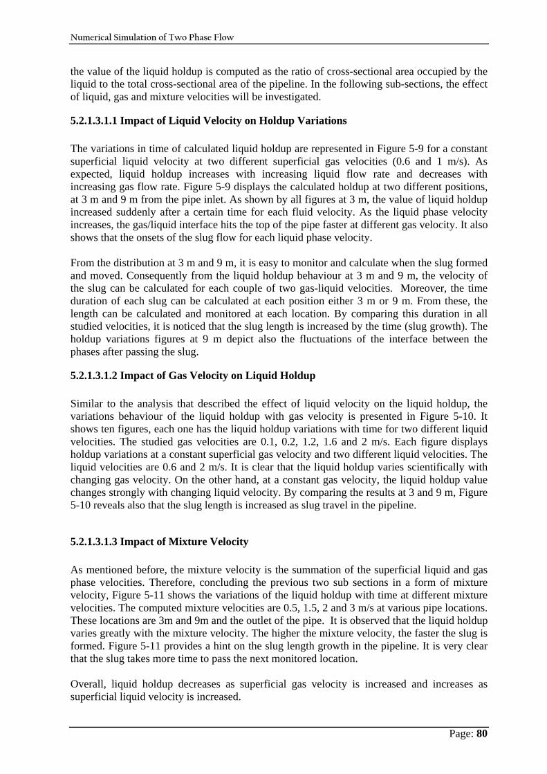
Numerical Simulation of Two Phase Flow

Page: 80

the value of the liquid holdup is computed as the ratio of cross-sectional area occupied by the liquid to the total cross-sectional area of the pipeline. In the following sub-sections, the effect of liquid, gas and mixture velocities will be investigated.

5.2.1.3.1.1 Impact of Liquid Velocity on Holdup Variations The variations in time of calculated liquid holdup are represented in Figure 5-9 for a constant superficial liquid velocity at two different superficial gas velocities (0.6 and 1 m/s). As expected, liquid holdup increases with increasing liquid flow rate and decreases with increasing gas flow rate. Figure 5-9 displays the calculated holdup at two different positions, at 3 m and 9 m from the pipe inlet. As shown by all figures at 3 m, the value of liquid holdup increased suddenly after a certain time for each fluid velocity. As the liquid phase velocity increases, the gas/liquid interface hits the top of the pipe faster at different gas velocity. It also shows that the onsets of the slug flow for each liquid phase velocity. From the distribution at 3 m and 9 m, it is easy to monitor and calculate when the slug formed and moved. Consequently from the liquid holdup behaviour at 3 m and 9 m, the velocity of the slug can be calculated for each couple of two gas-liquid velocities. Moreover, the time duration of each slug can be calculated at each position either 3 m or 9 m. From these, the length can be calculated and monitored at each location. By comparing this duration in all studied velocities, it is noticed that the slug length is increased by the time (slug growth). The holdup variations figures at 9 m depict also the fluctuations of the interface between the phases after passing the slug.

5.2.1.3.1.2 Impact of Gas Velocity on Liquid Holdup Similar to the analysis that described the effect of liquid velocity on the liquid holdup, the variations behaviour of the liquid holdup with gas velocity is presented in Figure 5-10. It shows ten figures, each one has the liquid holdup variations with time for two different liquid velocities. The studied gas velocities are 0.1, 0.2, 1.2, 1.6 and 2 m/s. Each figure displays holdup variations at a constant superficial gas velocity and two different liquid velocities. The liquid velocities are 0.6 and 2 m/s. It is clear that the liquid holdup varies scientifically with changing gas velocity. On the other hand, at a constant gas velocity, the liquid holdup value changes strongly with changing liquid velocity. By comparing the results at 3 and 9 m, Figure 5-10 reveals also that the slug length is increased as slug travel in the pipeline.

5.2.1.3.1.3 Impact of Mixture Velocity As mentioned before, the mixture velocity is the summation of the superficial liquid and gas phase velocities. Therefore, concluding the previous two sub sections in a form of mixture velocity, Figure 5-11 shows the variations of the liquid holdup with time at different mixture velocities. The computed mixture velocities are 0.5, 1.5, 2 and 3 m/s at various pipe locations. These locations are 3m and 9m and the outlet of the pipe. It is observed that the liquid holdup varies greatly with the mixture velocity. The higher the mixture velocity, the faster the slug is formed. Figure 5-11 provides a hint on the slug length growth in the pipeline. It is very clear that the slug takes more time to pass the next monitored location. Overall, liquid holdup decreases as superficial gas velocity is increased and increases as superficial liquid velocity is increased.

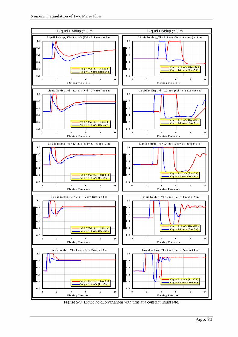
Numerical Simulation of Two Phase Flow

Page: 81

Liquid Holdup @ 3 m Liquid Holdup @ 9 m Liq u id h o ld u p _ Vl = 0 . 8 m/s (Vs l = 0 . 4 m/s ) a t 3 m

0 . 0

0 . 2

0 . 4

0 . 6

0 . 8

1. 0

0 2 4 6 8 10Flo win g Time , s e c

Vs g = 0 . 6 m/s (Ru n 3 2 )Vs g = 1. 0 m/s (Ru n 5 0 )

Liq u id h o ld u p _ Vl = 0 . 8 m/s (Vs l = 0 . 4 m/ s ) a t 9 m

0 . 0

0 . 2

0 . 4

0 . 6

0 . 8

1. 0

0 2 4 6 8 10Flo win g Time , s e c

Vs g = 0 . 6 m/s (Ru n 3 2 )Vs g = 1. 0 m/s (Ru n 5 0 )

Liq u id h o ld u p _ Vl = 1. 2 m/s (Vs l = 0 . 6 m/s ) a t 3 m

0 . 0

0 . 2

0 . 4

0 . 6

0 . 8

1. 0

0 2 4 6 8 10Flo win g Time , s e c

Vs g = 0 . 6 m/s (Ru n 3 3 )Vs g = 1. 0 m/s (Ru n 5 1)

Liq u id h o ld u p _ Vl = 1. 2 m/s (Vs l = 0 . 6 m/s ) a t 9 m

0 . 0

0 . 2

0 . 4

0 . 6

0 . 8

1. 0

0 2 4 6 8 10Flo win g Time , s e c

Vs g = 0 . 6 m/s (Ru n 3 3 )Vs g = 1. 0 m/s (Ru n 5 1)

Liq u id h o ld u p _ Vl = 1. 4 m/ s (Vs l = 0 . 7 m/ s ) a t 3 m

0 . 0

0 . 2

0 . 4

0 . 6

0 . 8

1. 0

0 2 4 6 8 10Flo win g Time , s e c

Vs g = 0 . 6 m/s (Ru n 3 4 )Vs g = 1. 0 m/s (Ru n 5 2 )

Liq u id h o ld u p _ Vl = 1. 4 m/s (Vs l = 0 . 7 m/s ) a t 9 m

0 . 0

0 . 2

0 . 4

0 . 6

0 . 8

1. 0

0 2 4 6 8 10Flo win g Time , s e c

Vs g = 0 . 6 m/s (Ru n 3 4 )Vs g = 1. 0 m/s (Ru n 5 2 )

Liq u id h o ld u p _ Vl = 2 m/s (Vs l = 1m/s ) a t 3 m

0 . 0

0 . 2

0 . 4

0 . 6

0 . 8

1. 0

0 2 4 6 8 10Flo win g Time , s e c

Vs g = 0 . 6 m/s (Ru n 3 5 )Vs g = 1. 0 m/s (Ru n 5 3 )

Liq u id h o ld u p _ Vl = 2 m/ s (Vs l = 1 m/ s ) a t 9 m

0 . 0

0 . 2

0 . 4

0 . 6

0 . 8

1. 0

0 2 4 6 8 10Flo win g Time , s e c

Vs g = 0 . 6 m/ s (Ru n 3 5 )Vs g = 1. 0 m/ s (Ru n 5 3 )

Liq u id h o ld u p _ Vl = 4 m/s (Vs l = 2 m/s ) a t 3 m

0 . 0

0 . 2

0 . 4

0 . 6

0 . 8

1. 0

0 2 4 6 8 10Flo win g Time , s e c

Vs g = 0 . 6 m/s (Ru n 3 6 )Vs g = 1. 0 m/s (Ru n 5 4 )

Liq u id h o ld u p _ Vl = 4 m/ s (Vs l = 2 m/s ) a t 9 m

0 . 0

0 . 2

0 . 4

0 . 6

0 . 8

1. 0

0 2 4 6 8 10Flo win g Time , s e c

Vs g = 0 . 6 m/s (Ru n 3 6 )Vs g = 1. 0 m/ s (Ru n 5 4 )

Figure 5-9: Liquid holdup variations with time at a constant liquid rate.

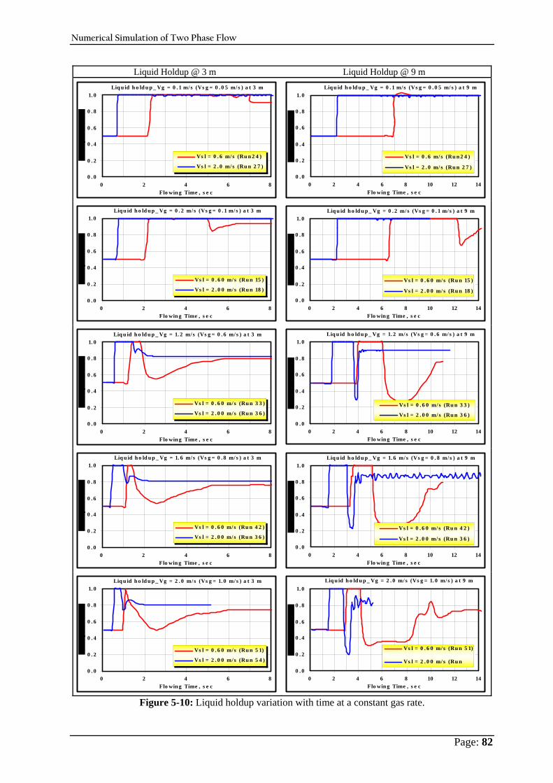
Numerical Simulation of Two Phase Flow

Page: 82

Liquid Holdup @ 3 m Liquid Holdup @ 9 m Liq u id h o ld u p _ Vg = 0 . 1 m/s (Vs g = 0 . 0 5 m/s ) a t 3 m

0 . 0

0 . 2

0 . 4

0 . 6

0 . 8

1. 0

0 2 4 6 8Flo win g Time , s e c

Vs l = 0 . 6 m/s (Ru n 2 4 )

Vs l = 2 . 0 m/s (Ru n 2 7 )

Liq u id h o ld u p _ Vg = 0 . 1 m/s (Vs g = 0 . 0 5 m/ s ) a t 9 m

0 . 0

0 . 2

0 . 4

0 . 6

0 . 8

1. 0

0 2 4 6 8 10 12 14Flo win g Time , s e c

Vs l = 0 . 6 m/ s (Ru n 2 4 )

Vs l = 2 . 0 m/ s (Ru n 2 7 )

Liq u id h o ld u p _ Vg = 0 . 2 m/ s (Vs g = 0 . 1 m/ s ) a t 3 m

0 . 0

0 . 2

0 . 4

0 . 6

0 . 8

1. 0

0 2 4 6 8Flo win g Time , s e c

Vs l = 0 . 6 0 m/ s (Ru n 15 )

Vs l = 2 . 0 0 m/ s (Ru n 18 )

Liq u id h o ld u p _ Vg = 0 . 2 m/ s (Vs g = 0 . 1 m/s ) a t 9 m

0 . 0

0 . 2

0 . 4

0 . 6

0 . 8

1. 0

0 2 4 6 8 10 12 14Flo win g Time , s e c

Vs l = 0 . 6 0 m/s (Ru n 15 )

Vs l = 2 . 0 0 m/s (Ru n 18 )

Liq u id h o ld u p _ Vg = 1. 2 m/s (Vs g = 0 . 6 m/s ) a t 3 m

0 . 0

0 . 2

0 . 4

0 . 6

0 . 8

1. 0

0 2 4 6 8Flo win g Time , s e c

Vs l = 0 . 6 0 m/s (Ru n 3 3 )

Vs l = 2 . 0 0 m/s (Ru n 3 6 )

Liq u id h o ld u p _ Vg = 1. 2 m/s (Vs g = 0 . 6 m/s ) a t 9 m

0 . 0

0 . 2

0 . 4

0 . 6

0 . 8

1. 0

0 2 4 6 8 10 12 14Flo win g Time , s e c

Vs l = 0 . 6 0 m/s (Ru n 3 3 )

Vs l = 2 . 0 0 m/s (Ru n 3 6 )

Liq u id h o ld u p _ Vg = 1. 6 m/s (Vs g = 0 . 8 m/ s ) a t 3 m

0 . 0

0 . 2

0 . 4

0 . 6

0 . 8

1. 0

0 2 4 6 8Flo win g Time , s e c

Vs l = 0 . 6 0 m/ s (Ru n 4 2 )

Vs l = 2 . 0 0 m/ s (Ru n 3 6 )

Liq u id h o ld u p _ Vg = 1. 6 m/s (Vs g = 0 . 8 m/s ) a t 9 m

0 . 0

0 . 2

0 . 4

0 . 6

0 . 8

1. 0

0 2 4 6 8 10 12 14Flo win g Time , s e c

Vs l = 0 . 6 0 m/ s (Ru n 4 2 )

Vs l = 2 . 0 0 m/ s (Ru n 3 6 )

Liq u id h o ld u p _ Vg = 2 . 0 m/s (Vs g = 1. 0 m/s ) a t 3 m

0 . 0

0 . 2

0 . 4

0 . 6

0 . 8

1. 0

0 2 4 6 8Flo win g Time , s e c

Vs l = 0 . 6 0 m/s (Ru n 5 1)

Vs l = 2 . 0 0 m/s (Ru n 5 4 )

Liq u id h o ld u p _ Vg = 2 . 0 m/s (Vs g = 1. 0 m/s ) a t 9 m

0 . 0

0 . 2

0 . 4

0 . 6

0 . 8

1. 0

0 2 4 6 8 10 12 14Flo win g Time , s e c

Vs l = 0 . 6 0 m/s (Ru n 5 1)

Vs l = 2 . 0 0 m/s (Ru n5 4 )

Figure 5-10: Liquid holdup variation with time at a constant gas rate.

Numerical Simulation of Two Phase Flow

Page: 83

Liquid holdup at 3m

0.0

0.2

0.4

0.6

0.8

1.0

0 2 4 6 8 10 12Flowing Time, sec

Holdup, Fraction

Vm = 0.5 m/sVm =1.5 m/sVm = 2.0 m/sVm = 3.0 m/s

Liquid holdup at 9m

0.0

0.2

0.4

0.6

0.8

1.0

0 2 4 6 8 10 12Flowing Time, sec

Holdup, Fraction

Vm = 0.5 m/sVm =1.5 m/sVm = 2.0 m/sVm = 3.0 m/s

Figure 5-11: The effect of mixture velocity on liquid holdup variations.

5.2.1.3.2 Liquid Film Level of Slug Unit The slug structure which occurs in a pipeline consists of a region of liquid with entrained gases, referred to as the liquid slug body, a gas bubble or pocket, and a liquid film. The liquid film height was monitored for each slugging run. It is found that this level depends on the liquid and gas phase velocities. The relation is plotted in Figure 5-12. On the contrary of stratified flow, it is observed that the height of the film varies strongly with changes of the liquid superficial velocity and gas superficial velocity. It is also observed that the equilibrium liquid film is not constant and strongly dependent on the flow rates of the prevailing fluids. In other words, the height of the liquid film in the gas pocket zone increases with liquid velocity. At a constant liquid velocity, the liquid film level has a direct relationship to the gas velocity. Indeed, the level of the liquid film in the gas pocket zone is not constant in each slug unit and it varies also from one slug to another. The value presented here is only for the first monitored slug unit and the level is the minimum liquid level in the bubble zone. Therefore, it would be incorrect to simplify the slug flowing model by using a constant liquid film in the gas pocket zone.

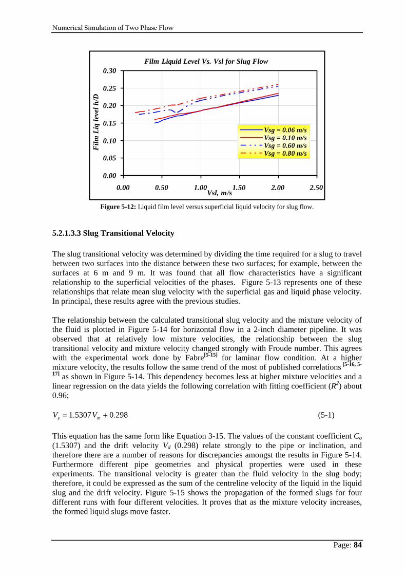
Numerical Simulation of Two Phase Flow

Page: 84

Film Liquid Level Vs. Vsl for Slug Flow

0.00

0.05

0.10

0.15

0.20

0.25

0.30

0.00 0.50 1.00 1.50 2.00 2.50Vsl, m/s

Film

Liq

leve

l h/D

Vsg = 0.06 m/sVsg = 0.10 m/sVsg = 0.60 m/sVsg = 0.80 m/s

Figure 5-12: Liquid film level versus superficial liquid velocity for slug flow.

5.2.1.3.3 Slug Transitional Velocity The slug transitional velocity was determined by dividing the time required for a slug to travel between two surfaces into the distance between these two surfaces; for example, between the surfaces at 6 m and 9 m. It was found that all flow characteristics have a significant relationship to the superficial velocities of the phases. Figure 5-13 represents one of these relationships that relate mean slug velocity with the superficial gas and liquid phase velocity. In principal, these results agree with the previous studies. The relationship between the calculated transitional slug velocity and the mixture velocity of the fluid is plotted in Figure 5-14 for horizontal flow in a 2-inch diameter pipeline. It was observed that at relatively low mixture velocities, the relationship between the slug transitional velocity and mixture velocity changed strongly with Froude number. This agrees with the experimental work done by Fabre[ 5-15] for laminar flow condition. At a higher mixture velocity, the results follow the same trend of the most of published correlations [ 5-16, 5-

17] as shown in Figure 5-14. This dependency becomes less at higher mixture velocities and a linear regression on the data yields the following correlation with fitting coefficient (R2) about 0.96;

298.05307.1 += ms V V (5-1) This equation has the same form like Equation 3-15. The values of the constant coefficient Co (1.5307) and the drift velocity Vd (0.298) relate strongly to the pipe or inclination, and therefore there are a number of reasons for discrepancies amongst the results in Figure 5-14. Furthermore different pipe geometries and physical properties were used in these experiments. The transitional velocity is greater than the fluid velocity in the slug body; therefore, it could be expressed as the sum of the centreline velocity of the liquid in the liquid slug and the drift velocity. Figure 5-15 shows the propagation of the formed slugs for four different runs with four different velocities. It proves that as the mixture velocity increases, the formed liquid slugs move faster.

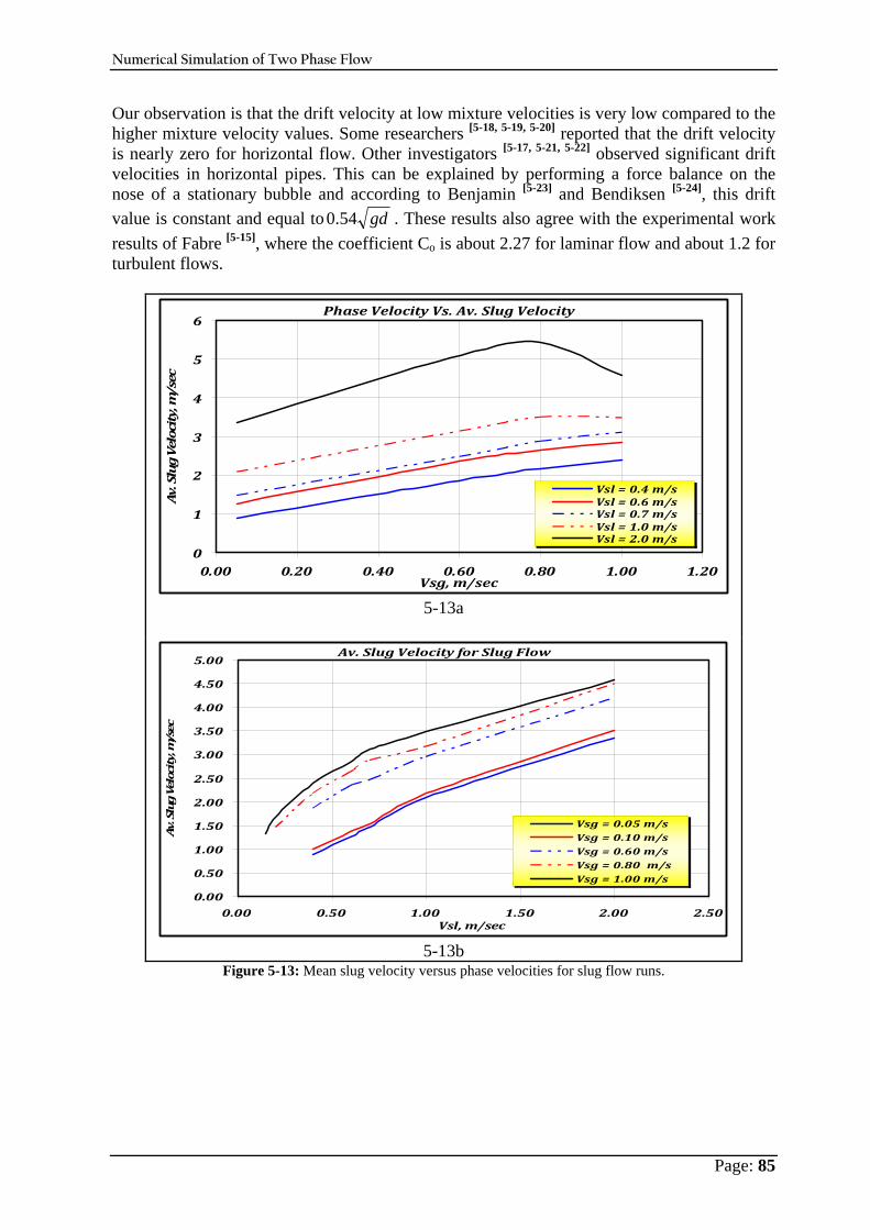
Numerical Simulation of Two Phase Flow

Page: 85

Our observation is that the drift velocity at low mixture velocities is very low compared to the higher mixture velocity values. Some researchers [ 5-18, 5-19, 5-20] reported that the drift velocity is nearly zero for horizontal flow. Other investigators [ 5-17, 5-21, 5-22] observed significant drift velocities in horizontal pipes. This can be explained by performing a force balance on the nose of a stationary bubble and according to Benjamin [ 5-23] and Bendiksen [ 5-24], this drift value is constant and equal to gd54.0 . These results also agree with the experimental work results of Fabre [ 5-15], where the coefficient Co is about 2.27 for laminar flow and about 1.2 for turbulent flows.

Phase Velocity Vs. Av. Slug Velocity

0

1

2

3

4

5

6

0.00 0.20 0.40 0.60 0.80 1.00 1.20Vsg, m/sec

Av. Slug Velocity, m/sec

Vsl = 0.4 m/sVsl = 0.6 m/sVsl = 0.7 m/sVsl = 1.0 m/sVsl = 2.0 m/s

5-13a

Av. Slug Velocity for Slug Flow

0.00

0.50

1.00

1.50

2.00

2.50

3.00

3.50

4.00

4.50

5.00

0.00 0.50 1.00 1.50 2.00 2.50Vsl, m/sec

Av. Slug Velocity, m/sec

Vsg = 0.05 m/sVsg = 0.10 m/sVsg = 0.60 m/sVsg = 0.80  m/sVsg = 1.00 m/s

5-13b Figure 5-13: Mean slug velocity versus phase velocities for slug flow runs.

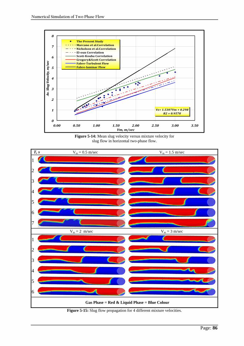
Numerical Simulation of Two Phase Flow

Page: 86

Vs= 1.5307Vm + 0.298R2 = 0.9578

0

1

2

3

4

5

6

7

8

0.00 0.50 1.00 1.50 2.00 2.50 3.00 3.50Vm, m/sec

Av. Slug Velocity, m/sec

The Present StudyMarcano et al.CorrelationNicholson et al.CorrelationEl­oun CorrelationScott­Kouba CorrelationGregory&Scott CorrelationFabre­Turbulent FlowFabre­laminar Flow

Figure 5-14: Mean slug velocity versus mixture velocity for

slug flow in horizontal two-phase flow.

T, s Vm = 0.5 m/sec Vm = 1.5 m/sec

1 2 3 4 5 6 7 Vm = 2 m/sec Vm = 3 m/sec

1 2 3 4 5 6 Gas Phase = Red & Liquid Phase = Blue Colour

Figure 5-15: Slug flow propagation for 4 different mixture velocities.

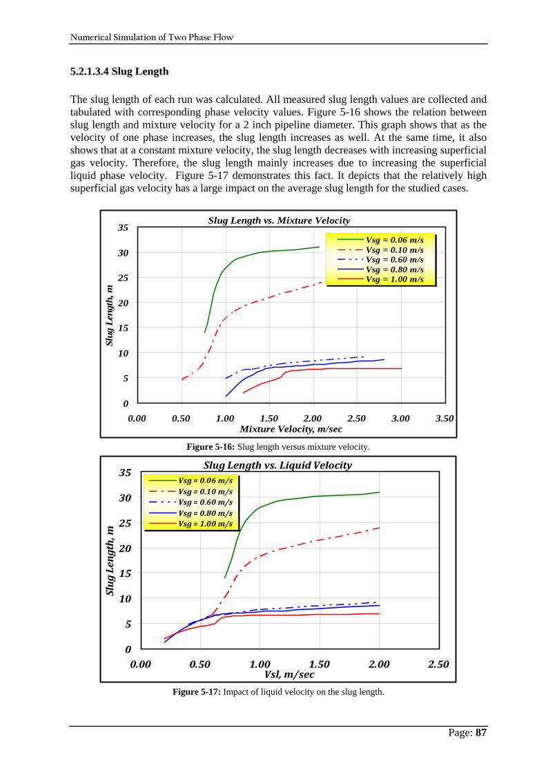
Numerical Simulation of Two Phase Flow

Page: 87

5.2.1.3.4 Slug Length The slug length of each run was calculated. All measured slug length values are collected and tabulated with corresponding phase velocity values. Figure 5-16 shows the relation between slug length and mixture velocity for a 2 inch pipeline diameter. This graph shows that as the velocity of one phase increases, the slug length increases as well. At the same time, it also shows that at a constant mixture velocity, the slug length decreases with increasing superficial gas velocity. Therefore, the slug length mainly increases due to increasing the superficial liquid phase velocity. Figure 5-17 demonstrates this fact. It depicts that the relatively high superficial gas velocity has a large impact on the average slug length for the studied cases.

Slug Length vs. Mixture Velocity

0

5

10

15

20

25

30

35

0.00 0.50 1.00 1.50 2.00 2.50 3.00 3.50Mixture Velocity, m/sec

Slug

Len

gth,

m

Vsg = 0.06 m/sVsg = 0.10 m/sVsg = 0.60 m/sVsg = 0.80 m/sVsg = 1.00 m/s

Figure 5-16: Slug length versus mixture velocity.

Slug Length vs. Liquid Velocity

0

5

10

15

20

25

30

35

0.00 0.50 1.00 1.50 2.00 2.50Vsl, m/sec

Slug Length, m

  

Vsg = 0.06 m/sVsg = 0.10 m/sVsg = 0.60 m/sVsg = 0.80 m/sVsg = 1.00 m/s

Figure 5-17: Impact of liquid velocity on the slug length.

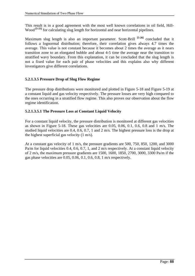
Numerical Simulation of Two Phase Flow

Page: 88

This result is in a good agreement with the most well known correlations in oil field, Hill-Wood [ 5-25] for calculating slug length for horizontal and near horizontal pipelines. Maximum slug length is also an important parameter. Scott-Brill [ 5-26] concluded that it follows a lognormal distribution; therefore, their correlation gives always 4.7 times the average. This value is not constant because it becomes about 2 times the average as it nears transition zone to an elongated bubble and about 4-5 time the average near the transition to stratified wavy boundary. From this explanation, it can be concluded that the slug length is not a fixed value for each pair of phase velocities and this explains also why different investigators give different correlations.

5.2.1.3.5 Pressure Drop of Slug Flow Regime The pressure drop distributions were monitored and plotted in Figure 5-18 and Figure 5-19 at a constant liquid and gas velocity respectively. The pressure losses are very high compared to the ones occurring in a stratified flow regime. This also proves our observation about the flow regime identification.

5.2.1.3.5.1 The Pressure Loss at Constant Liquid Velocity For a constant liquid velocity, the pressure distribution is monitored at different gas velocities as shown in Figure 5-18. These gas velocities are 0.05, 0.06, 0.1, 0.6, 0.8 and 1 m/s. The studied liquid velocities are 0.4, 0.6, 0.7, 1 and 2 m/s. The highest pressure loss is the drop at the highest superficial gas velocity (1 m/s). At a constant gas velocity of 1 m/s, the pressure gradients are 500, 750, 850, 1200, and 3000 Pa/m for liquid velocities 0.4, 0.6, 0.7, 1, and 2 m/s respectively. At a constant liquid velocity of 2 m/s, the maximum pressure gradients are 1500, 1600, 1850, 2700, 3000, 3300 Pa/m if the gas phase velocities are 0.05, 0.06, 0.1, 0.6, 0.8, 1 m/s respectively.

Numerical Simulation of Two Phase Flow

Page: 89

Slug Flow: Vsl = 0.40 m/sec

0

100

200

300

400

500

600

0 2 4 6 8 10Flowing Time, sec

dP/d

X, Pa/

m

Vsg = 0.05 m/s­Run 23Vsg = 0.06 m/s­Run 05Vsg = 0.10 m/s­Run 14Vsg = 0.60 m/s­Run 32Vsg = 0.80 m/s­Run 41Vsg = 1.00 m/s­Run 50

Slug Flow: Vsl = 0.60 m/sec

0

100

200

300

400

500

600

700

800

900

0 2 4 6 8 10Flowing Time, sec

dP/d

X, Pa/

m

Vsg = 0.05 m/s­Run 24Vsg = 0.06 m/s­Run 06Vsg = 0.10 m/s­Run 15Vsg = 0.60 m/s­Run 33Vsg = 0.80 m/s­Run 42Vsg = 1.00 m/s­Run 51

Slug Flow: Vsl = 0.70 m/sec

0

100

200

300

400

500

600

700

800

900

1000

0 2 4 6 8 10Flowing Time, sec

dP/d

X, Pa/

m

Vsg = 0.05 m/s­Run 25Vsg = 0.06 m/s­Run 07Vsg = 0.10 m/s­Run 16Vsg = 0.60 m/s­Run 34Vsg = 0.80 m/s­Run 43Vsg = 1.00 m/s­Run 52

Slug Flow: Vsl = 1.0 m/sec

0

200

400

600

800

1000

1200

1400

0 2 4 6 8 10Flowing Time, sec

dP/d

X, Pa/

m

Vsg = 0.05 m/s­Run 26Vsg = 0.06 m/s­Run 08Vsg = 0.10 m/s­Run 17Vsg = 0.60 m/s­Run 35Vsg = 0.80 m/s­Run 44Vsg = 1.00 m/s­Run 53

Slug Flow: Vsl = 2.0 m/sec

0

500

1000

1500

2000

2500

3000

3500

4000

0 2 4 6 8 10Flowing Time, sec

dP/d

X, Pa/

m

Vsg = 0.05 m/s­Run 27Vsg = 0.06 m/s­Run 09Vsg = 0.10 m/s­Run 18Vsg = 0.60 m/s­Run 36Vsg = 0.80 m/s­Run 45Vsg = 1.00 m/s­Run 54

Figure 5-18: Pressure gradient versus flowing time at constant liquid rates.

5.2.1.3.5.2 The Pressure Loss at Constant Gas Velocity The same observation was sketched for a constant gas velocity as displayed in Figure 5-19. The highest pressure drop was noticed at the highest liquid velocity at a constant gas velocity. This is also valid for all plotted gas velocities. This indicates that the pressure drop is strongly dependent on the liquid velocity. In conclusion, for a slug flow regime the gas phase velocity has a large impact on the pressure gradient along with the liquid phase velocity.

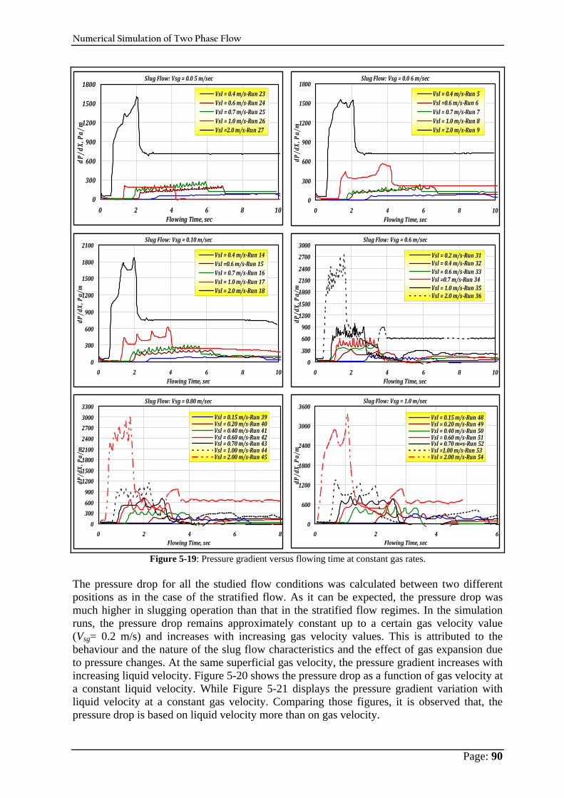
Numerical Simulation of Two Phase Flow

Page: 90

Slug Flow: Vsg = 0.0 5 m/sec

0

300

600

900

1200

1500

1800

0 2 4 6 8 10Flowing Time, sec

dP/d

X, Pa/

m

Vsl = 0.4 m/s­Run 23Vsl = 0.6 m/s­Run 24Vsl = 0.7 m/s­Run 25Vsl = 1.0 m/s­Run 26Vsl =2.0 m/s­Run 27

Slug Flow: Vsg = 0.0 6 m/sec

0

300

600

900

1200

1500

1800

0 2 4 6 8 10Flowing Time, sec

dP/dX, P

a/m

Vsl = 0.4 m/s­Run 5Vsl =0.6 m/s­Run 6Vsl = 0.7 m/s­Run 7Vsl = 1.0 m/s­Run 8Vsl = 2.0 m/s­Run 9

Slug Flow: Vsg = 0.10 m/sec

0

300

600

900

1200

1500

1800

2100

0 2 4 6 8 10Flowing Time, sec

dP/dX, P

a/m

Vsl = 0.4 m/s­Run 14Vsl =0.6 m/s­Run 15Vsl = 0.7 m/s­Run 16Vsl = 1.0 m/s­Run 17Vsl = 2.0 m/s­Run 18

Slug Flow: Vsg = 0.6 m/sec

0

300

600

900

1200

1500

1800

2100

2400

2700

3000

0 2 4 6 8 10Flowing Time, sec

dP/dX, P

a/m

Vsl = 0.2 m/s­Run 31Vsl = 0.4 m/s­Run 32Vsl = 0.6 m/s­Run 33Vsl =0.7 m/s­Run 34Vsl = 1.0 m/s­Run 35Vsl = 2.0 m/s­Run 36

Slug Flow: Vsg = 0.80 m/sec

0

300

600

900

1200

1500

1800

2100

2400

2700

3000

3300

0 2 4 6 8Flowing Time, sec

dP/dX, P

a/m

Vsl = 0.15 m/s­Run 39Vsl = 0.20 m/s­Run 40Vsl = 0.40 m/s­Run 41Vsl = 0.60 m/s­Run 42Vsl = 0.70 m/s­Run 43Vsl = 1.00 m/s­Run 44Vsl = 2.00 m/s­Run 45

Slug Flow: Vsg = 1.0 m/sec

0

600

1200

1800

2400

3000

3600

0 2 4 6Flowing Time, sec

dP/dX, P

a/m

Vsl = 0.15 m/s­Run 48Vsl = 0.20 m/s­Run 49Vsl = 0.40 m/s­Run 50Vsl = 0.60 m/s­Run 51Vsl = 0.70 m=s­Run 52Vsl =1.00 m/s­Run 53Vsl = 2.00 m/s­Run 54

Figure 5-19: Pressure gradient versus flowing time at constant gas rates. The pressure drop for all the studied flow conditions was calculated between two different positions as in the case of the stratified flow. As it can be expected, the pressure drop was much higher in slugging operation than that in the stratified flow regimes. In the simulation runs, the pressure drop remains approximately constant up to a certain gas velocity value (Vsg= 0.2 m/s) and increases with increasing gas velocity values. This is attributed to the behaviour and the nature of the slug flow characteristics and the effect of gas expansion due to pressure changes. At the same superficial gas velocity, the pressure gradient increases with increasing liquid velocity. Figure 5-20 shows the pressure drop as a function of gas velocity at a constant liquid velocity. While Figure 5-21 displays the pressure gradient variation with liquid velocity at a constant gas velocity. Comparing those figures, it is observed that, the pressure drop is based on liquid velocity more than on gas velocity.

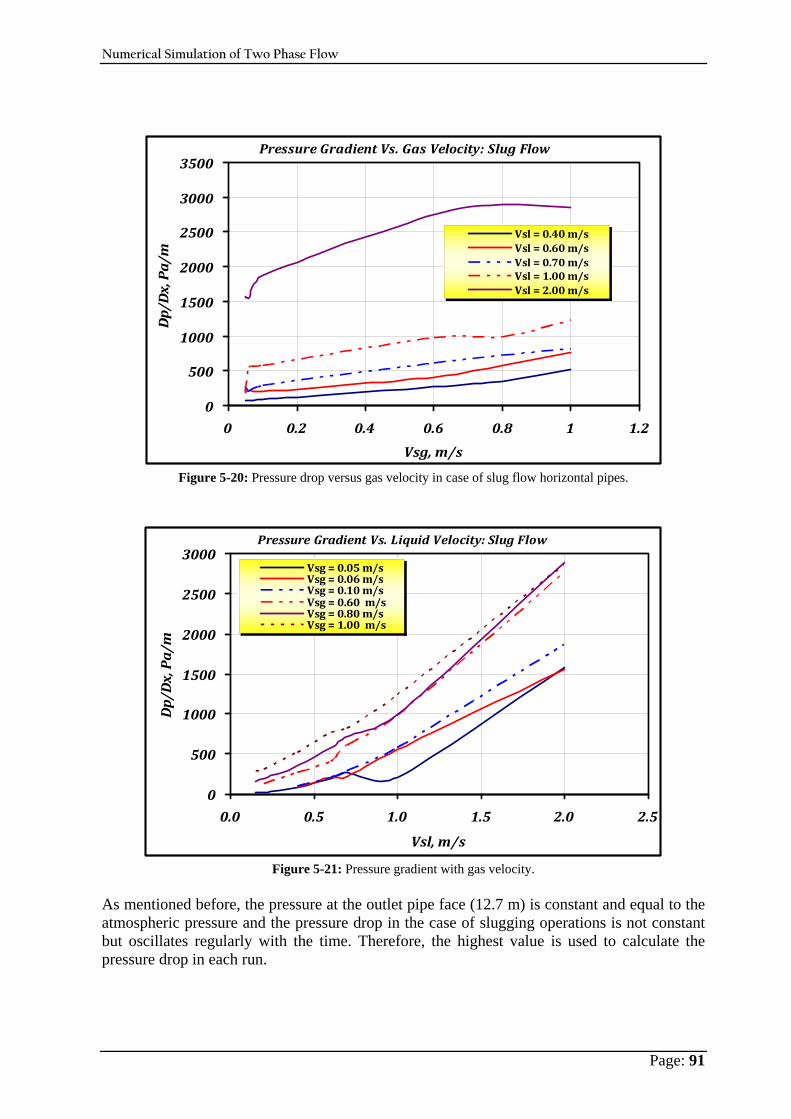
Numerical Simulation of Two Phase Flow

Page: 91

Pressure Gradient Vs. Gas Velocity: Slug Flow

0

500

1000

1500

2000

2500

3000

3500

0 0.2 0.4 0.6 0.8 1 1.2

Vsg, m/s

Dp/Dx, Pa/m

Vsl = 0.40 m/sVsl = 0.60 m/sVsl = 0.70 m/sVsl = 1.00 m/sVsl = 2.00 m/s

Figure 5-20: Pressure drop versus gas velocity in case of slug flow horizontal pipes.

Pressure Gradient Vs. Liquid Velocity: Slug Flow

0

500

1000

1500

2000

2500

3000

0.0 0.5 1.0 1.5 2.0 2.5

Vsl, m/s

Dp/Dx, Pa/m

Vsg = 0.05 m/sVsg = 0.06 m/sVsg = 0.10 m/sVsg = 0.60  m/sVsg = 0.80 m/sVsg = 1.00  m/s

Figure 5-21: Pressure gradient with gas velocity.

As mentioned before, the pressure at the outlet pipe face (12.7 m) is constant and equal to the atmospheric pressure and the pressure drop in the case of slugging operations is not constant but oscillates regularly with the time. Therefore, the highest value is used to calculate the pressure drop in each run.

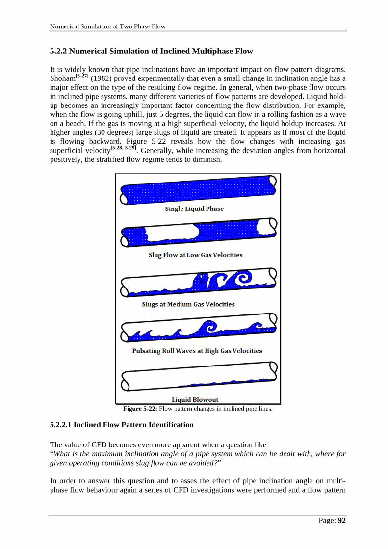
Numerical Simulation of Two Phase Flow

Page: 92

5.2.2 Numerical Simulation of Inclined Multiphase Flow It is widely known that pipe inclinations have an important impact on flow pattern diagrams. Shoham[ 5-27] (1982) proved experimentally that even a small change in inclination angle has a major effect on the type of the resulting flow regime. In general, when two-phase flow occurs in inclined pipe systems, many different varieties of flow patterns are developed. Liquid hold-up becomes an increasingly important factor concerning the flow distribution. For example, when the flow is going uphill, just 5 degrees, the liquid can flow in a rolling fashion as a wave on a beach. If the gas is moving at a high superficial velocity, the liquid holdup increases. At higher angles (30 degrees) large slugs of liquid are created. It appears as if most of the liquid is flowing backward. Figure 5-22 reveals how the flow changes with increasing gas superficial velocity[ 5-28, 5-29]. Generally, while increasing the deviation angles from horizontal positively, the stratified flow regime tends to diminish.

Figure 5-22: Flow pattern changes in inclined pipe lines.

5.2.2.1 Inclined Flow Pattern Identification The value of CFD becomes even more apparent when a question like “What is the maximum inclination angle of a pipe system which can be dealt with, where for given operating conditions slug flow can be avoided?” In order to answer this question and to asses the effect of pipe inclination angle on multi-phase flow behaviour again a series of CFD investigations were performed and a flow pattern

Numerical Simulation of Two Phase Flow

Page: 93

diagram was derived therefrom. With exception of the pipe inclination angle all boundary and operating conditions were kept the same as in the horizontal pipe case already discussed. The resulting flow pattern diagram is depicted in Figure 5-23. It shows for a pipe inclination angle of +5 degree a dramatic change in flow characteristics when compared to the horizontal pipe case (see Figure 5-4). It can be observed that there is no stratified flow regime existing any more and most of the area that corresponds to stratified flow conditions in the horizontal flow map now pertains to slug flow conditions. This figure compares well with what Shoham[ 5-27] found experimentally.

Figure 5-23: Flow pattern diagram for +5° pipe inclination angle constructed from CFD-results.

5.2.2.2 Impact of Phase Velocity on Holdup

5.2.2.2.1 Impact of Liquid Velocity on Holdup Variations In inclined pipes, the holdup profile was monitored for all the performed experiments at four locations in the pipeline, at 3 m, 6 m, 9 m and 12.7 m. The holdup distributions at 3m and 9m will be presented here only. Figure 5-24 shows the variations of the holdup for different liquid velocity. The studied superficial liquid velocities are 0.4 m/s, 0.6 m/s, 0.7 m/s and 2 m/s. At each liquid velocity, the gas velocity was changed to see the effects of the changing gas rate on the interface between the two phases. The pertinent superficial gas velocities are 0.1 and 0.6 m/s. At a constant superficial gas velocity, the changing of liquid velocity has a great effect on the profile of the holdup either at 3 or 9 m spots. At a high liquid velocity of 2 m/s, the holdup distribution differs significantly to those at lower superficial liquid velocities. In addition to that, at 3m position, a great number of pseudo slugs is noticed. Not all of them are capable to survive and reach the 9 m position. Therefore, by comparing any slug at 3 and 9 m, it is obvious that the slug length increased greatly (more than double in some cases) for lower

Numerical Simulation of Two Phase Flow

Page: 94

liquid velocities. The number of slugs is 8 for Vsg = 0.6 and Vsl = 0.7 m/s and 4 for Vsg = 0.6 and Vsl = 0.6, i.e. increasing liquid velocity by about 0.1 m/s, the number of slugs has been increased from 4 to 8 slugs in inclined two phase flow.

VOF_3m:  Vsl = 0.40 m/s

0.0

0.2

0.4

0.6

0.8

1.0

0 2 4 6 8 10Flowing time, sec

Liquid Holdup, %

Vsg = 0.100 m/sVsg = 0.600m/s

VOF_9m:  Vsl = 0.40 m/s

0.0

0.2

0.4

0.6

0.8

1.0

0 2 4 6 8 10 12 14 16 18 20Flowing time, sec

Liquid Holdup, %

Vsg = 0.100 m/sVsg = 0.600m/s

VOF_3m:  Vsl = 0.60 m/s

0.0

0.2

0.4

0.6

0.8

1.0

0 2 4 6 8 10Flowing time, sec

Liquid Holdup, %

Vsg = 0.10 m/sVsg = 0.60 m/s

VOF_9m:  Vsl = 0.60 m/s

0.0

0.2

0.4

0.6

0.8

1.0

0 2 4 6 8 10 12 14 16 18 20Flowing time, sec

Liquid Holdup, %

Vsg = 0.10 m/sVsg = 0.60 m/s

VOF_3m:  Vsl = 0.70 m/s

0.0

0.2

0.4

0.6

0.8

1.0

0 2 4 6 8 10Flowing time, sec

Liquid Holdup, %

Vsg = 0.10 m/sVsg = 0.60 m/s

VOF_9m:  Vsl = 0.70 m/s

0.0

0.2

0.4

0.6

0.8

1.0

0 2 4 6 8 10 12 14 16 18 20Flowing time, sec

Liquid Holdup, %

Vsg = 0.10 m/sVsg = 0.60 m/s

VOF_3m:  Vsl = 2.0 m/s

0.0

0.2

0.4

0.6

0.8

1.0

0 2 4 6 8 10Flowing time, sec

Liquid Holdup, %

Vsg = 0.10 m/sVsg = 0.60 m/s

VOF_9m:  Vsl = 2.0 m/s

0.0

0.2

0.4

0.6

0.8

1.0

0 2 4 6 8 10 12 14 16 18 20Flowing time, sec

Liquid Holdup, %

Vsg = 0.10 m/sVsg = 0.60 m/s

Figure 5-24: Effect of liquid rate on liquid holdup.

5.2.2.2.2 Impact of Gas Velocity on Liquid Holdup Like previous investigation about the effect of liquid velocity on holdup, gas velocity has been studied and the results are calculated and plotted in Figure 5-25. In addition to each studied gas velocity, liquid velocity was varied to depict the effect of liquid velocity on the holdup. It is noticed that at lower gas velocities (0.06, 0.1 m/s), the effect of gas rate on liquid holdup is approximately constant. As the gas phase velocity increases, the effects become significant at a constant liquid velocity and a lot of pseudo slugs are formed and disappeared.

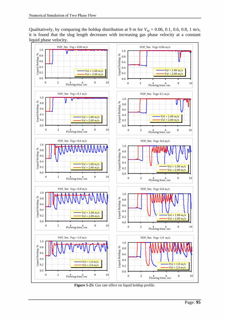
Numerical Simulation of Two Phase Flow

Page: 95

Qualitatively, by comparing the holdup distribution at 9 m for Vsg = 0.06, 0.1, 0.6, 0.8, 1 m/s, it is found that the slug length decreases with increasing gas phase velocity at a constant liquid phase velocity.

VOF_3m:  Vsg = 0.06 m/s

0.0

0.2

0.4

0.6

0.8

1.0

0 2 4 6 8 10Flowing time, sec

Liquid Holdup, %

Vsl = 1.00 m/sVsl = 2.00 m/s

VOF_9m:  Vsg= 0.06 m/s

0.0

0.2

0.4

0.6

0.8

1.0

0 2 4 6 8 10Flowing time, sec

Liquid Holdup, %

Vsl = 1.00 m/sVsl = 2.00 m/s

VOF_3m:  Vsg = 0.1 m/s

0.0

0.2

0.4

0.6

0.8

1.0

0 2 4 6 8 10Flowing time, sec

Liquid Holdup, %

Vsl = 1.00 m/sVsl = 2.00 m/s

VOF_9m:  Vsg= 0.1 m/s

0.0

0.2

0.4

0.6

0.8

1.0

0 2 4 6 8 10Flowing time, sec

Liquid Holdup, %

Vsl = 1.00 m/sVsl = 2.00 m/s

VOF_3m:  Vsg = 0.6 m/s

0.0

0.2

0.4

0.6

0.8

1.0

0 2 4 6 8 10Flowing time, sec

Liquid Holdup, %

Vsl = 1.00 m/sVsl = 2.00 m/s

VOF_9m:  Vsg= 0.6 m/s

0.0

0.2

0.4

0.6

0.8

1.0

0 2 4 6 8 10Flowing time, sec

Liquid Holdup, %

Vsl = 1.00 m/sVsl = 2.00 m/s

VOF_3m:  Vsg = 0.8 m/s

0.0

0.2

0.4

0.6

0.8

1.0

0 2 4 6 8 10Flowing time, sec

Liquid Holdup, %

Vsl = 1.00 m/sVsl = 2.00 m/s

VOF_9m:  Vsg= 0.8 m/s

0.0

0.2

0.4

0.6

0.8

1.0

0 2 4 6 8 10Flowing time, sec

Liquid Holdup, %

Vsl = 1.00 m/sVsl = 2.00 m/s

VOF_3m:  Vsg = 1.0 m/s

0.0

0.2

0.4

0.6

0.8

1.0

0 2 4 6 8 10Flowing time, sec

Liquid Holdup, %

Vsl = 1.0 m/sVsl = 2.0 m/s

VOF_9m:  Vsg= 1.0  m/s

0.0

0.2

0.4

0.6

0.8

1.0

0 2 4 6 8 10Flowing time, sec

Liquid Holdup, %

Vsl = 1.0 m/sVsl = 2.0 m/s

Figure 5-25: Gas rate effect on liquid holdup profile.

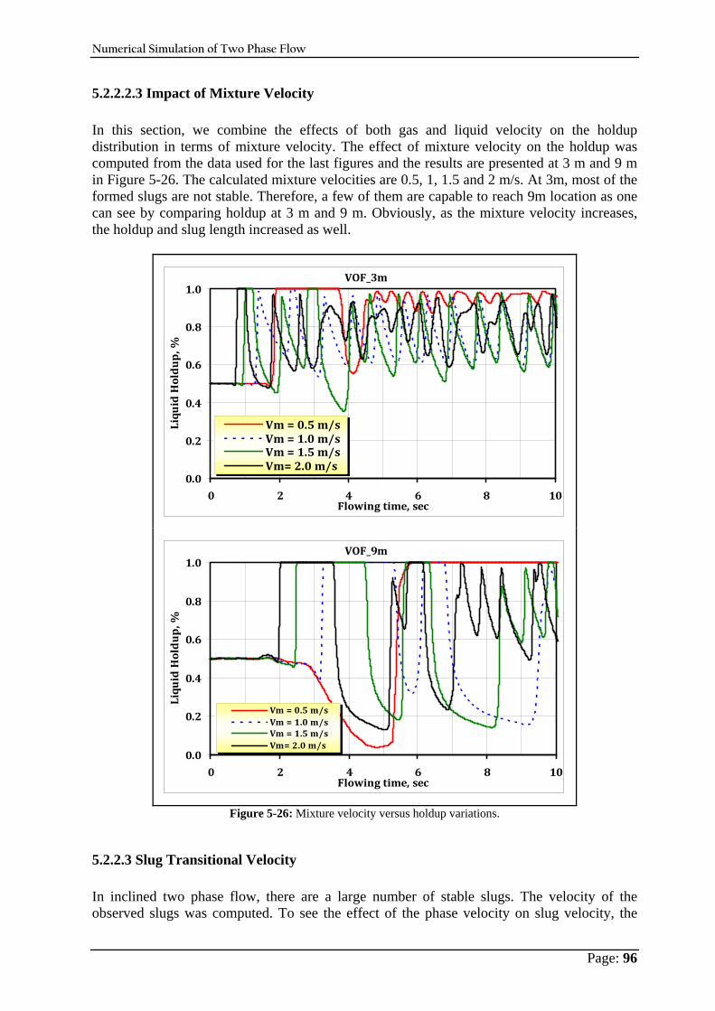
Numerical Simulation of Two Phase Flow

Page: 96

5.2.2.2.3 Impact of Mixture Velocity In this section, we combine the effects of both gas and liquid velocity on the holdup distribution in terms of mixture velocity. The effect of mixture velocity on the holdup was computed from the data used for the last figures and the results are presented at 3 m and 9 m in Figure 5-26. The calculated mixture velocities are 0.5, 1, 1.5 and 2 m/s. At 3m, most of the formed slugs are not stable. Therefore, a few of them are capable to reach 9m location as one can see by comparing holdup at 3 m and 9 m. Obviously, as the mixture velocity increases, the holdup and slug length increased as well.

VOF_3m 

0.0

0.2

0.4

0.6

0.8

1.0

0 2 4 6 8 10Flowing time, sec

Liquid Holdup, %

Vm = 0.5 m/sVm = 1.0 m/sVm = 1.5 m/sVm= 2.0 m/s

VOF_9m 

0.0

0.2

0.4

0.6

0.8

1.0

0 2 4 6 8 10Flowing time, sec

Liquid Holdup, %

Vm = 0.5 m/sVm = 1.0 m/sVm = 1.5 m/sVm= 2.0 m/s

Figure 5-26: Mixture velocity versus holdup variations.

5.2.2.3 Slug Transitional Velocity In inclined two phase flow, there are a large number of stable slugs. The velocity of the observed slugs was computed. To see the effect of the phase velocity on slug velocity, the

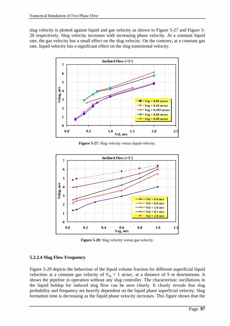
Numerical Simulation of Two Phase Flow

Page: 97

slug velocity is plotted against liquid and gas velocity as shown in Figure 5-27 and Figure 5-28 respectively. Slug velocity increases with increasing phase velocity. At a constant liquid rate, the gas velocity has a small effect on the slug velocity. On the contrary, at a constant gas rate, liquid velocity has a significant effect on the slug transitional velocity.

Inclined Flow (+5°)

0

1

2

3

4

5

6

7

0.0 0.5 1.0 1.5 2.0 2.5Vsl, m/s

Vsl

ug, m

/s

Vsg = 0.06 m/secVsg = 0.10 m/secVsg = 0.305 m/secVsg = 0.60 m/secVsg = 0.80 m/sec

Figure 5-27: Slug velocity versus liquid velocity.

Inclined Flow (+5°)

0

1

2

3

4

5

6

7

0.0 0.2 0.4 0.6 0.8 1.0 1.2Vsg, m/s

Vsl

ug, m

/s

Vsl = 0.4 m/sVsl = 0.6 m/sVsl = 1.0 m/sVsl = 0.7 m/sVsl = 2.0 m/s

Figure 5-28: Slug velocity versus gas velocity.

5.2.2.4 Slug Flow Frequency Figure 5-29 depicts the behaviour of the liquid volume fraction for different superficial liquid velocities at a constant gas velocity of Vsg = 1 m/sec, at a distance of 9 m downstream. It shows the pipeline in operation without any slug controller. The characteristic oscillations in the liquid holdup for induced slug flow can be seen clearly. It clearly reveals that slug probability and frequency are heavily dependent on the liquid phase superficial velocity. Slug formation time is decreasing as the liquid phase velocity increases. This figure shows that the

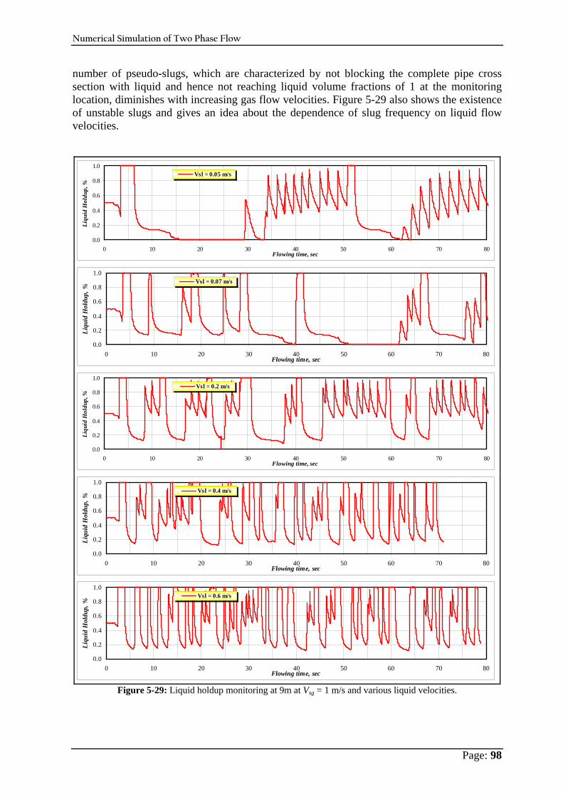
Numerical Simulation of Two Phase Flow

Page: 98

number of pseudo-slugs, which are characterized by not blocking the complete pipe cross section with liquid and hence not reaching liquid volume fractions of 1 at the monitoring location, diminishes with increasing gas flow velocities. Figure 5-29 also shows the existence of unstable slugs and gives an idea about the dependence of slug frequency on liquid flow velocities.

0.0

0.2

0.4

0.6

0.8

1.0

0 10 20 30 40 50 60 70 80Flowing time, sec

Liqu

id H

oldu

p, %

Vsl = 0.05 m/s

0.0

0.2

0.4

0.6

0.8

1.0

0 10 20 30 40 50 60 70 80Flowing time, sec

Liqu

id H

oldu

p, %

Vsl = 0.07 m/s

0.0

0.2

0.4

0.6

0.8

1.0

0 10 20 30 40 50 60 70 80Flowing time, sec

Liqu

id H

oldu

p, %

Vsl = 0.2 m/s

0.0

0.2

0.4

0.6

0.8

1.0

0 10 20 30 40 50 60 70 80Flowing time, sec

Liqu

id H

oldu

p, %

Vsl = 0.4 m/s

0.0

0.2

0.4

0.6

0.8

1.0

0 10 20 30 40 50 60 70 80Flowing time, sec

Liqu

id H

oldu

p, %

Vsl = 0.6 m/s

Figure 5-29: Liquid holdup monitoring at 9m at Vsg = 1 m/s and various liquid velocities.

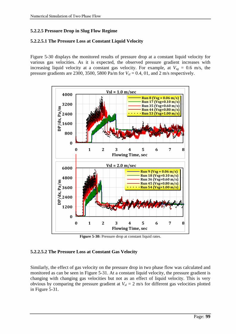
Numerical Simulation of Two Phase Flow

Page: 99

5.2.2.5 Pressure Drop in Slug Flow Regime

5.2.2.5.1 The Pressure Loss at Constant Liquid Velocity

Figure 5-30 displays the monitored results of pressure drop at a constant liquid velocity for various gas velocities. As it is expected, the observed pressure gradient increases with increasing liquid velocity at a constant gas velocity. For example, at Vsg = 0.6 m/s, the pressure gradients are 2300, 3500, 5800 Pa/m for Vsl = 0.4, 01, and 2 m/s respectively.

Vsl = 1.0 m/sec

0

800

1600

2400

3200

4000

0 1 2 3 4 5 6 7 8Flowing Time, sec

DP/dx, Pa/m

Run 8 (Vsg = 0.06 m/s)Run 17 (Vsg=0.10 m/s)Run 35 (Vsg=0.60 m/s)Run 44 (Vsg=0.80 m/s)Run 53 (Vsg=1.00 m/s)

Vsl = 2.0 m/sec

0

1200

2400

3600

4800

6000

0 1 2 3 4 5 6 7 8Flowing Time, sec

DP/dx, Pa/m

Run 9 (Vsg = 0.06 m/s)Run 18 (Vsg=0.10 m/s)Run 36 (Vsg=0.60 m/s)Run 45 (Vsg=0.80 m/s)Run 54 (Vsg=1.00 m/s)

Figure 5-30: Pressure drop at constant liquid rates.

5.2.2.5.2 The Pressure Loss at Constant Gas Velocity

Similarly, the effect of gas velocity on the pressure drop in two phase flow was calculated and monitored as can be seen in Figure 5-31. At a constant liquid velocity, the pressure gradient is changing with changing gas velocities but not as an effect of liquid velocity. This is very obvious by comparing the pressure gradient at Vsl = 2 m/s for different gas velocities plotted in Figure 5-31.

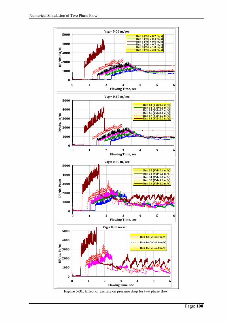
Numerical Simulation of Two Phase Flow

Page: 100

Vsg = 0.06 m/sec

0

1000

2000

3000

4000

5000

0 1 2 3 4 5 6Flowing Time, sec

DP/dx, Pa/m

Run 4 (Vsl = 0.2 m/s)Run 5 (Vsl = 0.4 m/s)Run 6 (Vsl = 0.6 m/s)Run 7 (Vsl = 0.7 m/s)Run 8 (Vsl = 1.0 m/s)Run 9 (Vsl = 2.0 m/s)

Vsg = 0.10 m/sec

0

1000

2000

3000

4000

5000

0 1 2 3 4 5 6Flowing Time, sec

DP/dx, Pa/m

Run 13 (Vsl=0.2 m/s)Run 14 (Vsl=0.4 m/s)Run 15 (Vsl=0.6 m/s)Run 16 (Vsl=0.7 m/s)Run 17 (Vsl=1.0 m/s)Run 18 (Vsl=2.0 m/s)

Vsg = 0.60 m/sec

0

1000

2000

3000

4000

5000

0 1 2 3 4 5 6Flowing Time, sec

DP/dx, Pa/m

Run 32 (Vsl=0.4 m/s)Run 33 (Vsl=0.6 m/s)Run 34 (Vsl=0.7 m/s)Run 35 (Vsl=1.0 m/s)Run 36 (Vsl=2.0 m/s)

Vsg = 0.80 m/sec

0

1000

2000

3000

4000

5000

0 1 2 3 4 5 6Flowing Time, sec

DP/dx, Pa/m

Run 43 (Vsl=0.7 m/s)

Run 44 (Vsl=1.0 m/s)

Run 45 (Vsl=2.0 m/s)

Figure 5-31: Effect of gas rate on pressure drop for two phase flow.

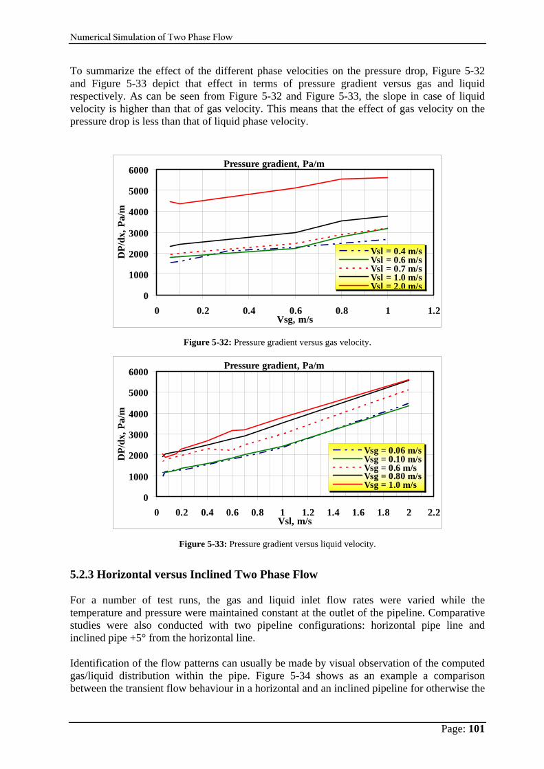
Numerical Simulation of Two Phase Flow

Page: 101

To summarize the effect of the different phase velocities on the pressure drop, Figure 5-32 and Figure 5-33 depict that effect in terms of pressure gradient versus gas and liquid respectively. As can be seen from Figure 5-32 and Figure 5-33, the slope in case of liquid velocity is higher than that of gas velocity. This means that the effect of gas velocity on the pressure drop is less than that of liquid phase velocity.

Pressure gradient, Pa/m

0

1000

2000

3000

4000

5000

6000

0 0.2 0.4 0.6 0.8 1 1.2Vsg, m/s

DP/

dx, P

a/m

Vsl = 0.4 m/sVsl = 0.6 m/sVsl = 0.7 m/sVsl = 1.0 m/sVsl = 2.0 m/s

Figure 5-32: Pressure gradient versus gas velocity.

Pressure gradient, Pa/m

0

1000

2000

3000

4000

5000

6000

0 0.2 0.4 0.6 0.8 1 1.2 1.4 1.6 1.8 2 2.2Vsl, m/s

DP/

dx, P

a/m

Vsg = 0.06 m/sVsg = 0.10 m/sVsg = 0.6 m/sVsg = 0.80 m/sVsg = 1.0 m/s

Figure 5-33: Pressure gradient versus liquid velocity.

5.2.3 Horizontal versus Inclined Two Phase Flow For a number of test runs, the gas and liquid inlet flow rates were varied while the temperature and pressure were maintained constant at the outlet of the pipeline. Comparative studies were also conducted with two pipeline configurations: horizontal pipe line and inclined pipe +5° from the horizontal line. Identification of the flow patterns can usually be made by visual observation of the computed gas/liquid distribution within the pipe. Figure 5-34 shows as an example a comparison between the transient flow behaviour in a horizontal and an inclined pipeline for otherwise the

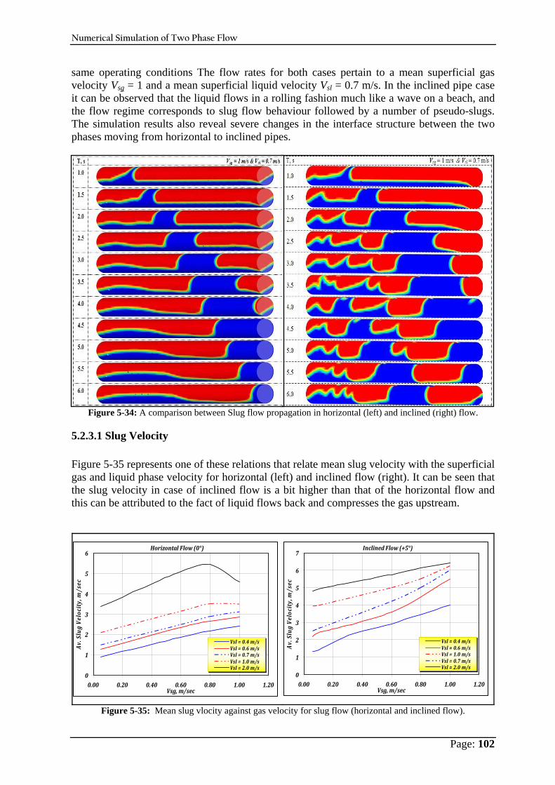
Numerical Simulation of Two Phase Flow

Page: 102

same operating conditions The flow rates for both cases pertain to a mean superficial gas velocity Vsg = 1 and a mean superficial liquid velocity Vsl = 0.7 m/s. In the inclined pipe case it can be observed that the liquid flows in a rolling fashion much like a wave on a beach, and the flow regime corresponds to slug flow behaviour followed by a number of pseudo-slugs. The simulation results also reveal severe changes in the interface structure between the two phases moving from horizontal to inclined pipes.

Figure 5-34: A comparison between Slug flow propagation in horizontal (left) and inclined (right) flow.

5.2.3.1 Slug Velocity Figure 5-35 represents one of these relations that relate mean slug velocity with the superficial gas and liquid phase velocity for horizontal (left) and inclined flow (right). It can be seen that the slug velocity in case of inclined flow is a bit higher than that of the horizontal flow and this can be attributed to the fact of liquid flows back and compresses the gas upstream.

Horizontal Flow (0°)

0

1

2

3

4

5

6

0.00 0.20 0.40 0.60 0.80 1.00 1.20Vsg, m/sec

Av. Slug Velocity, m/sec

Vsl = 0.4 m/sVsl = 0.6 m/sVsl = 0.7 m/sVsl = 1.0 m/sVsl = 2.0 m/s

Inclined Flow (+5°)

0

1

2

3

4

5

6

7

0.00 0.20 0.40 0.60 0.80 1.00 1.20Vsg, m/sec

Av. Slug Velocity, m/sec

Vsl = 0.4 m/sVsl = 0.6 m/sVsl = 1.0 m/sVsl = 0.7 m/sVsl = 2.0 m/s

Figure 5-35: Mean slug vlocity against gas velocity for slug flow (horizontal and inclined flow).

Numerical Simulation of Two Phase Flow

Page: 103

5.2.3.2 Slug Length Figure 5-36 shows the ratio of inclined to horizontal pipe slug length versus superficial gas velocity. The results are in good agreement with the experimental work of Zheng et al.[ 5-30]. In case of inclined flow (+5°), Zheng et al.[ 5-30] proved experimentally that the slug length variations range from 1.25 to 1.53 at Vsl = 0.6 m/s and for a Vsg ranges from 1 to 4.5 m/s.

0.00

0.20

0.40

0.60

0.80

1.00

1.20

1.40

1.60

1.80

0.00 0.20 0.40 0.60 0.80 1.00 1.20Vsg, m/s

Ls (+

5°)/L

s(0°

)

Figure 5-36: Average slug length variations.

5.2.3.3 Pressure Drop In Figure 5-37, the computed variation of pressure drop as a function of superficial gas velocity for horizontal and inclined flows is depicted. It is evident that due to the additional elevation gradient the pressure drop in case of inclined pipelines is much higher than for horizontal flows under the same operating conditions. In Figure 5-37 on the left diagram, also the pressure drop for stratified flow conditions which can be only be found in horizontal pipe flows is displayed.

Pressure gradient in horizontal two phase flow

0

1000

2000

3000

4000

5000

6000

0.00 0.20 0.40 0.60 0.80 1.00 1.20Vsg, m/s

DP/

Dx,

Pa/

m

0

2

4

6

8

10

12

DP/

Dx,

Pa/

m (D

otte

d lin

e)

Vs l = 0 . 4 0 m/sVs l = 0 . 6 0 m/sVs l = 0 . 7 0 m/sVs l = 1. 0 0 m/ sVs l = 2 . 0 0 m/svs l = 0 . 0 5 m/ svs l = 0 . 0 7 m/ svs l = 0 . 15 m/ s

Pressure gradient in inclined (+5°) two phase flow

0

1000

2000

3000

4000

5000

6000

0 0.2 0.4 0.6 0.8 1 1.2Vsg, m/s

DP/

dx, P

a/m

Vsl = 0.4 m/sVsl = 0.6 m/sVsl = 0.7 m/sVsl = 1.0 m/sVsl = 2.0 m/s

Figure 5-37: Pressure drop versus superficial gas velocity for horizontal and inclined pipes.

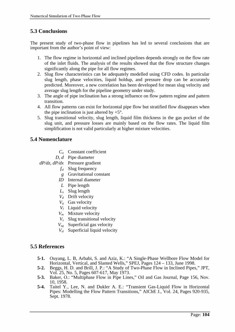
Numerical Simulation of Two Phase Flow

Page: 104

5.3 Conclusions The present study of two-phase flow in pipelines has led to several conclusions that are important from the author’s point of view:

1. The flow regime in horizontal and inclined pipelines depends strongly on the flow rate of the inlet fluids. The analysis of the results showed that the flow structure changes significantly along the pipe for all flow regimes.

2. Slug flow characteristics can be adequately modelled using CFD codes. In particular slug length, phase velocities, liquid holdup, and pressure drop can be accurately predicted. Moreover, a new correlation has been developed for mean slug velocity and average slug length for the pipeline geometry under study.

3. The angle of pipe inclination has a strong influence on flow pattern regime and pattern transition.

4. All flow patterns can exist for horizontal pipe flow but stratified flow disappears when the pipe inclination is just altered by +5°.

5. Slug transitional velocity, slug length, liquid film thickness in the gas pocket of the slug unit, and pressure losses are mainly based on the flow rates. The liquid film simplification is not valid particularly at higher mixture velocities.

5.4 Nomenclature

Co Constant coefficient D, d Pipe diameter

dP/dz, dP/dx Pressure gradient fsl Slug frequency g Gravitational constant

ID Internal diameter L Pipe length

Ls Slug length Vd Drift velocity Vg Gas velocity Vl Liquid velocity

Vm Mixture velocity Vs Slug transitional velocity

Vsg Superficial gas velocity Vsl Superficial liquid velocity

5.5 References

5-1. Ouyang, L. B, Arbabi, S. and Aziz, K.: “A Single-Phase Wellbore Flow Model for Horizontal, Vertical, and Slanted Wells,” SPEJ, Pages 124 – 133, June 1998.

5-2. Beggs, H. D. and Brill, J. P.: “A Study of Two-Phase Flow in Inclined Pipes,” JPT, Vol. 25, No. 5, Pages 607-617, May 1973.

5-3. Baker, O.: “Multiphase Flow in Pipe Lines,” Oil and Gas Journal, Page 156, Nov. 10, 1958.

5-4. Taitel Y., Lee, N. and Dukler A. E.: “Transient Gas-Liquid Flow in Horizontal Pipes: Modelling the Flow Pattern Transitions,” AIChE J., Vol. 24, Pages 920-935, Sept. 1978.

Numerical Simulation of Two Phase Flow

Page: 105

5-5. Taitel Y. and Dukler A. E.: “A Model for Prediction Flow Regime Transitions in Horizontal and Near Horizontal Gas-Liquid Flow,” AIChE J., Vol. 22, Issue 5, Pages 920-934, Jan. 1976.

5-6. Hewitt, G. F. and Hall-Taylor, N. S.: Annular Two Phase Flow, Pergamon Press, Oxford, UK, 1970.

5-7. Baker, O.: “Simultaneous Flow of Oil and Gas,” Oil & Gas J., Vol. 53, No. 2, Pages 185-195, July 1954.

5-8. Wilkens, R. J., Thomas, D. K. and Glassmeyer, S. R.: “Surfactant Use for Slug Flow Patterns Suppression and New Flow Patterns Types in a Horizontal Pipe,” Journal of Fluids Engineering, Vol. 128, No. 1, Pages 164-169, January 2006.

5-9. Fluent Inc., User’s Guide for Fluent 6.3, http:/www.fluent.com, Lebanon, NH, 2006.

5-10. Wilcox, D. C.: Turbulence Modeling for CFD, DCW Industries, Inc., La Canada, CA, 1993.

5-11. Weisman, J., Duncan, D., Gibson, J. and Crawford, T.: “Effects of Fluid Properties and Pipe Diameter on Two-Phase Flow Patterns in Horizontal Lines,” International Journal of Multiphase Flow, Vol. 5, No. 6 Pages 437-462, Dec.1979.

5-12. Mandhane, J. M., Gregory G. A. and Aziz, K.: “A Flow Pattern Map for Gas-Liquid Flow in Horizontal Pipes: Predictive Models,” International Journal of Multiphase Flow, Vol. 1, No.4, Pages 537-553, Oct. 1974.

5-13. Abduvayt, P., Arihara, N., Manabe and R. Ikeda, K.: “Experimental and Modelling Studies for Gas-Liquid Two-Phase Flow at High Pressure Conditions,” Journal of the Japan Petroleum Institute, Vol. 46, No.2, Pages 111-125, 2003.

5-14. Meng, W., Chen, X. T., Kouba, G. E., Sarica, C. and Brill, J. P. : “Experimental Study of Low Liquid Loading Gas-Liquid Flow in Near-Horizontal Pipes,” SPE Paper 56466, Presented at the 1999 SPE Annual Technical Conference and Exhibition held in Houston, Texas, 3-6, Oct. 1999.

5-15. Fabre, J.: “Advancements in Two-Phase Slug Flow Modeling,” SPE Paper 27961, Presented at the University of Tulsa Centennial Petroleum Engineering Symposium held in Tulsa, OK. USA, 29-31 Aug. 1994.

5-16. Marcano, R., Chen. X. T., Sarica, C. and Brill, J. P.: “A Study of Slug Characteristics for Two-Phase Horizontal Flow,” SPE 39856, International Petroleum Conference and Exhibition of Mexico, Villahermosa, 3-5 March 1998.

5-17. Nicholson, M. K., Aziz, K. and Gregory G. A.: “Intermittent Two-Phase Flow in Horizontal Pipes: Predictive Models,” Canadian Journal of Chemical Engineering, Vol. 56, Pages 653-663, 1978.

5-18. Dukler, A. E. and Hubbard, M. G.: “A Model for Gas-Liquid Slug Flow in Horizontal and Near Horizontal Tubes,” Ind. Eng. Chem. Fundam., Vol. 14, No. 4, pages 337-347, 1975.

5-19. Gregory G. A. and D. S. Scott: “Correlation of Liquid Slug Velocity and Frequency in Horizontal Co-current Gas-Liquid Slug Flow,” AIChE J., Vol. 15, No. 6, Pages 933-935, Nov. 1969.

5-20. Heywood, N I. and Richardson, J. F.: “Slug Flow of Air-Water Mixtures in a Horizontal Pipe: Determination of Liquid Holdup by γ-ray Absorption,” Chem. Eng. Sci., Vol. 34, No. 1, Pages 17-30. 1979.

5-21. Kouba, G. E.: Horizontal Slug Flow Modeling and Metering, Ph. D. Dissertation, the University of Tulsa, 1986.

5-22. Matter, L. and Gregory, G. A.: “Air-Oil Slug Flow in an Upward-Inclined Pipe-I: Slug Velocity, Holdup and Pressure Gradient,” J. Can. Technol., Vol. 13, Pages 69-76, 1974.

5-23. Benjamin, T. B.: “Gravity Currents and Related Phenomena,” J. Fluid Mech., Vol. 31, Pages 209-248, 1968.

5-24. Bendiksen, K. H.: “An Experimental Investigation of the Motion of Long Bubbles in Inclined Tubes,” International Journal of Multiphase Flow, Vol. 10, Issue 4, Pages 467-483, Aug. 1984.

5-25. Hirt, C. W. and Nichols, B. D.: “Volume of Fluid (VOF) Method for the Dynamics of Free Boundaries,” Journal of Computational Physics, Vol. 39, No. 1, Pages 201-225, 1981.

Numerical Simulation of Two Phase Flow

Page: 106

5-26. Scott, S. L., Shoham, O. and Brill, J. P.: “Prediction of Slug Length in Horizontal Large-Diameter Pipes,” SPE Paper 15103 & SPE Production Engineering, Pages 335-340, August 1989.

5-27. Shoham, O.: Flow Pattern Transitions and Characterization in Gas-Liquid Two Phase Flow in Inclined Pipes, Ph. D. Thesis, Tel-Aviv University, Ramat-Aviv, Israel, 1982.

5-28. Texas A & M: http://www.pe.utexas.edu/2phaseweb/flowinclin.html 5-29. Petalas N. and Aziz, K.: “A Mechanistic Model for Multiphase Flow in Pipe,”

Presented at the 49th Annual Technical Meeting of the Petroleum Society of the Canadian Institute of Mining, Metallurgy and Petroleum held in Calgary, Alberta, Canada on June 8-10, 1998.

5-30. Zheng, G. H., Brill, J. P. and Shoham, O.: “An Experimental Study of Two-Phase Slug Flow in Hilly Terrain Pipelines,” SPE Production and Facilities, Nov. 1995.

Matzen New Flow Assurance

Page: 107

CHAPTER VI

Matzen New Flow Assurance

6.1 The Problem: Project “Matzen Neu” The objective of the project “Matzen Neu” is to modernize the infrastructure of the Matzen field, which is located approximately 20 km north-east from Vienna. The project includes the construction of a new, central Gas/Oil Separation Plant (GOSP), which is replacing 12 existing stations and will simplify technical procedures considerably. The existing production stations will be adapted into gauging stations, serving for collection, volumetric flow measurement and transmission of the oil produced. The 60 km long pipeline necessary for this is also being renewed and optimized [ 6-1]. The part of the pipeline this study was done for connects the gathering and metering station Ma VI to the center GOSP (Figure 6-1) and has a length of about 2 km. The purpose of the study was – by using the CFD codes developed in this thesis- to design this part of pipeline systems to ensure slugging generating conditions are occurring. This study started by checking the flow regime using the previous analytical correlations for two different pipeline diameters (DN400 and DN450). Six different correlations have been used. Afterwards, the numerical work strategy was started by calculation of the liquid holdup at the beginning of the pipe, using eight different approaches. This was needed to define the actual velocities of the liquid and gas phases while the CFD code deals with the true velocities and not the superficial ones, as normally given. At the end, slug flow characteristics (slug transitional velocity, holdup, slug volume and slug frequency) and the pressure drop calculation have been calculated and analyzed for this pipeline.

6.2 Mechanical Solutions 6.2.1 Flow Regime Prediction Numerous studies have been carried out to describe two phase flow in horizontal, near horizontal and inclined pipelines. The analytical solutions are based on the most famous and accurate flow regime maps. The used maps are Beggs and Brill[ 6-1, 6-2], Weisman et al. [ 6-3], Mandhane et al. [ 6-4], Taitel and Dukler[ 6-5], and Petalas-Aziz[ 6-6]. Each flow map has its own parameters; all of these parameters have been calculated for MaVI-GOSP pipeline for both DN400 and DN450 and listed in Table 6-1 assuming the entire pipeline is horizontal or near horizontal.

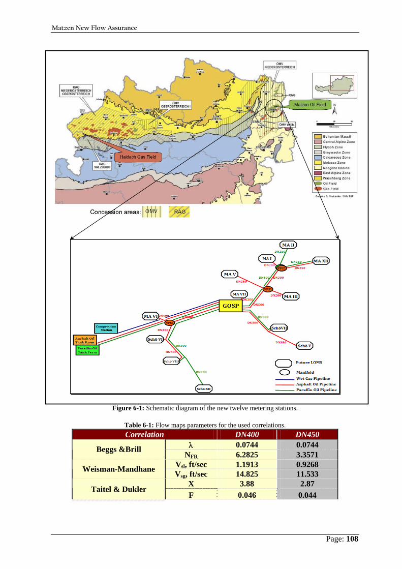
Matzen New Flow Assurance

Page: 108

Figure 6-1: Schematic diagram of the new twelve metering stations.

Table 6-1: Flow maps parameters for the used correlations. Correlation DN400 DN450

λ 0.0744 0.0744 Beggs &Brill NFR 6.2825 3.3571

Vsl, ft/sec 1.1913 0.9268 Weisman-Mandhane Vsg, ft/sec 14.825 11.533 X 3.88 2.87

Taitel & Dukler F 0.046 0.044

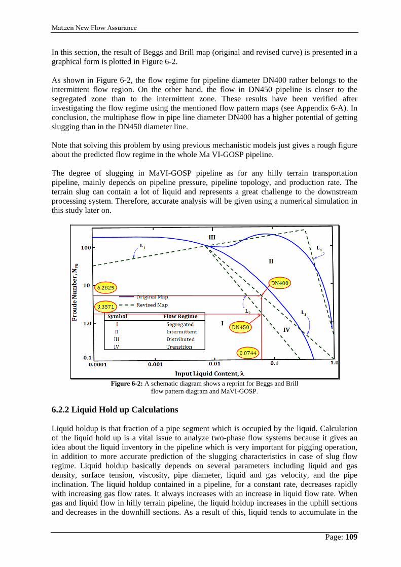
Matzen New Flow Assurance

Page: 109

In this section, the result of Beggs and Brill map (original and revised curve) is presented in a graphical form is plotted in Figure 6-2. As shown in Figure 6-2, the flow regime for pipeline diameter DN400 rather belongs to the intermittent flow region. On the other hand, the flow in DN450 pipeline is closer to the segregated zone than to the intermittent zone. These results have been verified after investigating the flow regime using the mentioned flow pattern maps (see Appendix 6-A). In conclusion, the multiphase flow in pipe line diameter DN400 has a higher potential of getting slugging than in the DN450 diameter line. Note that solving this problem by using previous mechanistic models just gives a rough figure about the predicted flow regime in the whole Ma VI-GOSP pipeline. The degree of slugging in MaVI-GOSP pipeline as for any hilly terrain transportation pipeline, mainly depends on pipeline pressure, pipeline topology, and production rate. The terrain slug can contain a lot of liquid and represents a great challenge to the downstream processing system. Therefore, accurate analysis will be given using a numerical simulation in this study later on.

Figure 6-2: A schematic diagram shows a reprint for Beggs and Brill

flow pattern diagram and MaVI-GOSP.

6.2.2 Liquid Hold up Calculations Liquid holdup is that fraction of a pipe segment which is occupied by the liquid. Calculation of the liquid hold up is a vital issue to analyze two-phase flow systems because it gives an idea about the liquid inventory in the pipeline which is very important for pigging operation, in addition to more accurate prediction of the slugging characteristics in case of slug flow regime. Liquid holdup basically depends on several parameters including liquid and gas density, surface tension, viscosity, pipe diameter, liquid and gas velocity, and the pipe inclination. The liquid holdup contained in a pipeline, for a constant rate, decreases rapidly with increasing gas flow rates. It always increases with an increase in liquid flow rate. When gas and liquid flow in hilly terrain pipeline, the liquid holdup increases in the uphill sections and decreases in the downhill sections. As a result of this, liquid tends to accumulate in the

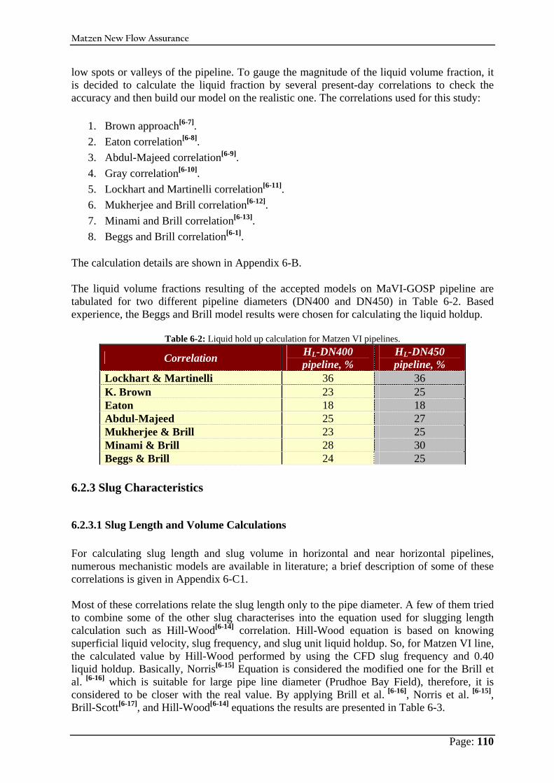
Matzen New Flow Assurance

Page: 110

low spots or valleys of the pipeline. To gauge the magnitude of the liquid volume fraction, it is decided to calculate the liquid fraction by several present-day correlations to check the accuracy and then build our model on the realistic one. The correlations used for this study:

1. Brown approach[ 6-7]. 2. Eaton correlation[ 6-8]. 3. Abdul-Majeed correlation[ 6-9]. 4. Gray correlation[ 6-10]. 5. Lockhart and Martinelli correlation[ 6-11]. 6. Mukherjee and Brill correlation[ 6-12]. 7. Minami and Brill correlation[ 6-13]. 8. Beggs and Brill correlation[ 6-1].

The calculation details are shown in Appendix 6-B. The liquid volume fractions resulting of the accepted models on MaVI-GOSP pipeline are tabulated for two different pipeline diameters (DN400 and DN450) in Table 6-2. Based experience, the Beggs and Brill model results were chosen for calculating the liquid holdup.

Table 6-2: Liquid hold up calculation for Matzen VI pipelines.

Correlation HL-DN400 pipeline, %

HL-DN450 pipeline, %

Lockhart & Martinelli 36 36 K. Brown 23 25 Eaton 18 18 Abdul-Majeed 25 27 Mukherjee & Brill 23 25 Minami & Brill 28 30 Beggs & Brill 24 25

6.2.3 Slug Characteristics

6.2.3.1 Slug Length and Volume Calculations For calculating slug length and slug volume in horizontal and near horizontal pipelines, numerous mechanistic models are available in literature; a brief description of some of these correlations is given in Appendix 6-C1. Most of these correlations relate the slug length only to the pipe diameter. A few of them tried to combine some of the other slug characterises into the equation used for slugging length calculation such as Hill-Wood[ 6-14] correlation. Hill-Wood equation is based on knowing superficial liquid velocity, slug frequency, and slug unit liquid holdup. So, for Matzen VI line, the calculated value by Hill-Wood performed by using the CFD slug frequency and 0.40 liquid holdup. Basically, Norris[ 6-15] Equation is considered the modified one for the Brill et al. [ 6-16] which is suitable for large pipe line diameter (Prudhoe Bay Field), therefore, it is considered to be closer with the real value. By applying Brill et al. [ 6-16], Norris et al. [ 6-15], Brill-Scott[ 6-17], and Hill-Wood[ 6-14] equations the results are presented in Table 6-3.

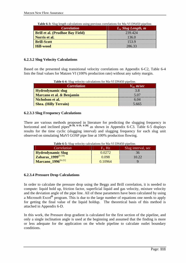
Matzen New Flow Assurance

Page: 111

Table 6-3: Slug length calculations using previous correlations for Ma-VI DN450 pipeline. Correlation Ls, Slug Length, m

Brill et al. (Prudhoe Bay Field) 239.424 Norris et al. 136.0 Brill-Scott 153.9 Hill-wood 286.33

6.2.3.2 Slug Velocity Calculations Based on the presented slug transitional velocity correlations on Appendix 6-C2, Table 6-4 lists the final values for Matzen VI (100% production rate) without any safety margin.

Table 6-4: Slug velocity calculations for Ma-VI DN450 pipeline. Correlation Vts, m/sec

Hydrodynamic slug 3.8 Marcano et al. & Benjamin 5.07 Nicholson et al. 6.04 Shea. (Hilly Terrain) 5.665

6.2.3.3 Slug Frequency Calculations There are various methods proposed in literature for predicting the slugging frequency in horizontal and inclined pipes[ 6-18, 6-19, 6-20] as shown in Appendix 6-C3. Table 6-5 displays results for the time cyclic (slugging interval) and slugging frequency for each slug unit observed on simulating MaVI GOSP pipe line at 100% production flowing.

Table 6-5: Slug velocity calculations for Ma-VI DN450 pipeline. Correlation Fs, Hz Slug interval, sec

Hydrodynamic Slug 0.0272 36 Zabaras_1999[ 6-19] 0.098 10.22 Marcano_1996[ 6-21] 0.10964 9

6.2.3.4 Pressure Drop Calculations In order to calculate the pressure drop using the Beggs and Brill correlation, it is needed to compute: liquid hold up, friction factor, superficial liquid and gas velocity, mixture velocity and the deviation angle of the pipe line. All of these parameters have been calculated by using a Microsoft Excel® program. This is due to the large number of equations one needs to apply for getting the final value of the liquid holdup. The theoretical basis of this method is attached in Appendix 6-D. In this work, the Pressure drop gradient is calculated for the first section of the pipeline, and only a single inclination angle is used at the beginning and assumed that the finding is more or less adequate for the application on the whole pipeline to calculate outlet boundary conditions.

Matzen New Flow Assurance

Page: 112

6.2.3.4.1 Pressure Drop ΔP-DN400 Based on Beggs and Brill pressure drop correlations, the pressure gradient for DN400 Matzen VI pipeline is about 38 Pa/m. Therefore, the total pressure drop in the whole 1863 m long MaVI-GOSP DN400 pipeline is calculated as follows:

( ) ( ) bar 0.71 Pa 70794 m 1863 Pa/m 38 ==×=ΔP (6-1) To proof these calculations, a shareware PipeDrop® software package was used to calculate the pressure gradient. It was found to be about 41 Pa/m, therefore, based on this result the pressure drop in the whole Matzen-VI DN400 was computed again to be:

( ) ( ) bar 0.76 Pa 76383 m 1863 Pa/m 41 ==×=ΔP (6-2)

6.2.3.4.2 Pressure Drop ΔP-DN450 Assuming the entire pipeline is approximately horizontal; the pressure loss has been calculated and was found to be 20 Pa/m. By using the inclination angle of the first segment as a fixed angle for the entire pipeline, the pressure drop has been found to be 24 Pa/m. Therefore, for the first pipeline segment under study, the pressure drop is about 2500 Pa, for the second pipeline segment is about 3300 Pa, and for the studied long-pipe (542m), the drop was about 13500 Pa. By considering the whole pipeline of MaVI-GOSP, the pressure drop is 44712 Pa (0.447 bar). Absolute pipeline roughness affects the pressure drop calculation significantly. So the absolute roughness used in the previous pressure drop calculations, is about 0.41 μm (given by OMV[ 6-1]) which considers the pipeline as absolutely smooth. The pressure loss calculations were performed with a modified Beggs and Brill correlation. Then the pressure value has been calculated at the outlet of the pipeline. The simulation work used this calculated pressure value as an outlet pressure.

6.3 Numerical Analysis 6.3.1 Boundary Conditions and Pipe Geometry By using CFD and VOF and after investigating the profile and the topology of the MaVI-GOSP pipeline starting from Live Oil Metering Station (LOMS) to the main GOSP, it is found that three sections of the pipeline have a higher probability of slugging. Therefore, these sections have been chosen for this study. The first pipe section is the pipe line from LOMS 130 m in the direction of flow towards the main separation station, the second selected section is starting after the fluid flows downhill and then directed uphill for about 164 m and the third one is combining all the pipe sections that have a large tendency to grow up the slugging. The third pipe length is about 542 m. The topology of the selected pipe line sections is shown in Figure 6-3, the geometry of these sections is shown in Figure 6-4 and Figure 6-5 depicts the interface and the grid resolution of the cross section of the pipe under investigation.

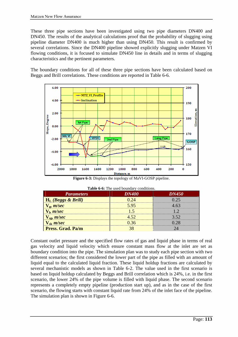
Matzen New Flow Assurance

Page: 113

These three pipe sections have been investigated using two pipe diameters DN400 and DN450. The results of the analytical calculations proof that the probability of slugging using pipeline diameter DN400 is much higher than using DN450. This result is confirmed by several correlations. Since the DN400 pipeline showed explicitly slugging under Matzen VI flowing conditions, it is focused to simulate DN450 line in details and in terms of slugging characteristics and the pertinent parameters. The boundary conditions for all of these three pipe sections have been calculated based on Beggs and Brill correlations. These conditions are reported in Table 6-6.

Figure 6-3: Displays the topology of MaVI-GOSP pipeline.

Table 6-6: The used boundary conditions.

Parameters DN400 DN450 HL (Beggs & Brill) 0.24 0.25 Vg, m/sec 5.95 4.63 Vl, m/sec 1.5 1.2 Vsg, m/sec 4.52 3.52 Vsl, m/sec 0.36 0.28 Press. Grad. Pa/m 38 24

Constant outlet pressure and the specified flow rates of gas and liquid phase in terms of real gas velocity and liquid velocity which ensure constant mass flow at the inlet are set as boundary condition into the pipe. The simulation plan was to study each pipe section with two different scenarios; the first considered the lower part of the pipe as filled with an amount of liquid equal to the calculated liquid fraction. These liquid holdup fractions are calculated by several mechanistic models as shown in Table 6-2. The value used in the first scenario is based on liquid holdup calculated by Beggs and Brill correlation which is 24%, i.e. in the first scenario, the lower 24% of the pipe volume is filled with liquid phase. The second scenario represents a completely empty pipeline (production start up), and as in the case of the first scenario, the flowing starts with constant liquid rate from 24% of the inlet face of the pipeline. The simulation plan is shown in Figure 6-6.

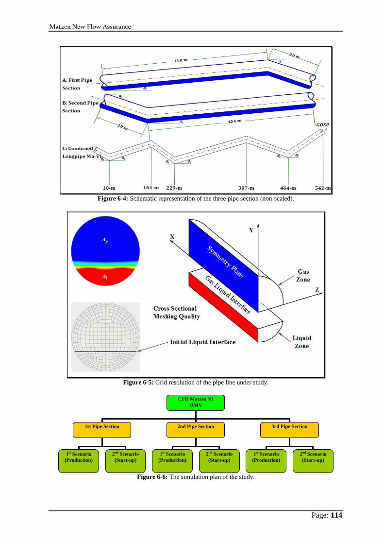
Matzen New Flow Assurance

Page: 114

Figure 6-4: Schematic representation of the three pipe section (non-scaled).

Figure 6-5: Grid resolution of the pipe line under study.

Figure 6-6: The simulation plan of the study.

CFD Matzen VI OMV

1st Pipe Section 2nd Pipe Section 3rd Pipe Section

1st Scenario (Production)

2nd Scenario (Start-up)

1st Scenario (Production)

2nd Scenario (Start-up)

1st Scenario (Production)

2nd Scenario (Start-up)

Matzen New Flow Assurance

Page: 115

Finite volume meshes and grid generation The FLUENT pre-processor GAMBIT was used to build the model geometries. Meshing was performed by first griding the cross-section at one end of the fluid domain and then extruding the mesh in the axial direction. For the slug flow simulations in the near horizontally inclined pipes, symmetry with respect to the vertical plane has been assumed. Therefore hexahedral meshes in a half cylinder have been generated each element of about 0.1 m length. In Figure 6-5, the meshing quality for the complete cross section is depicted. Geometrical dimensions and computational mesh details are given in Table 6-7.

Table 6-7: Grid resolution parameter for the simulation runs.

6.3.2 Simulation Results

6.3.2.1 First Pipe Section Simulations Figure 6-7 displays the schematic profile of the first tested pipe section and related boundary conditions and geometry details. The simulation work was performed under the boundary conditions that had been calculated using the real data given by OMV[ 6-1]. The pressure gauge values at end of the pipe section were calculated based on Beggs and Brill correlation. Table 6-8 summarises these boundary conditions and fluid properties.

Table 6-8: Boundary conditions for the simulated first pipe section.

Para. Vl, m/s

Vg, m/s

Pout, Pa

ρg, kg/m3

ρw, kg/m3

ρo, kg/m3 θ1 θ2

μw. Cst

μo, Cst

L, m

ID, mm

T, oC

HL, %

Calc. Value 1.177 4.626 305500 0.77 1013 911 +

0.06 -

0.925 1 52.6 130 438.15 30 25

This pipe section has been investigated under three different operating conditions, normal flowing by 100% flow rate capacity, then shut-in till all the fluids settled down and finally re-start flow under the same 100% flowing condition. The duration of each operating conditions is shown in Figure 6-8 for the first and second scenario. The impact of all of these transient operations is shown in the animated file saved in the attached CD.

Spatial mesh resolution Mesh description D,

mm L, Length,

m Grid/ cross section Grid/ Length

No. of grid cells

First pipe section 438 130 472 1300 613600 Second pipe section 438 164 440 1114 490360

Long pipe 438 542 206 5420 1116520

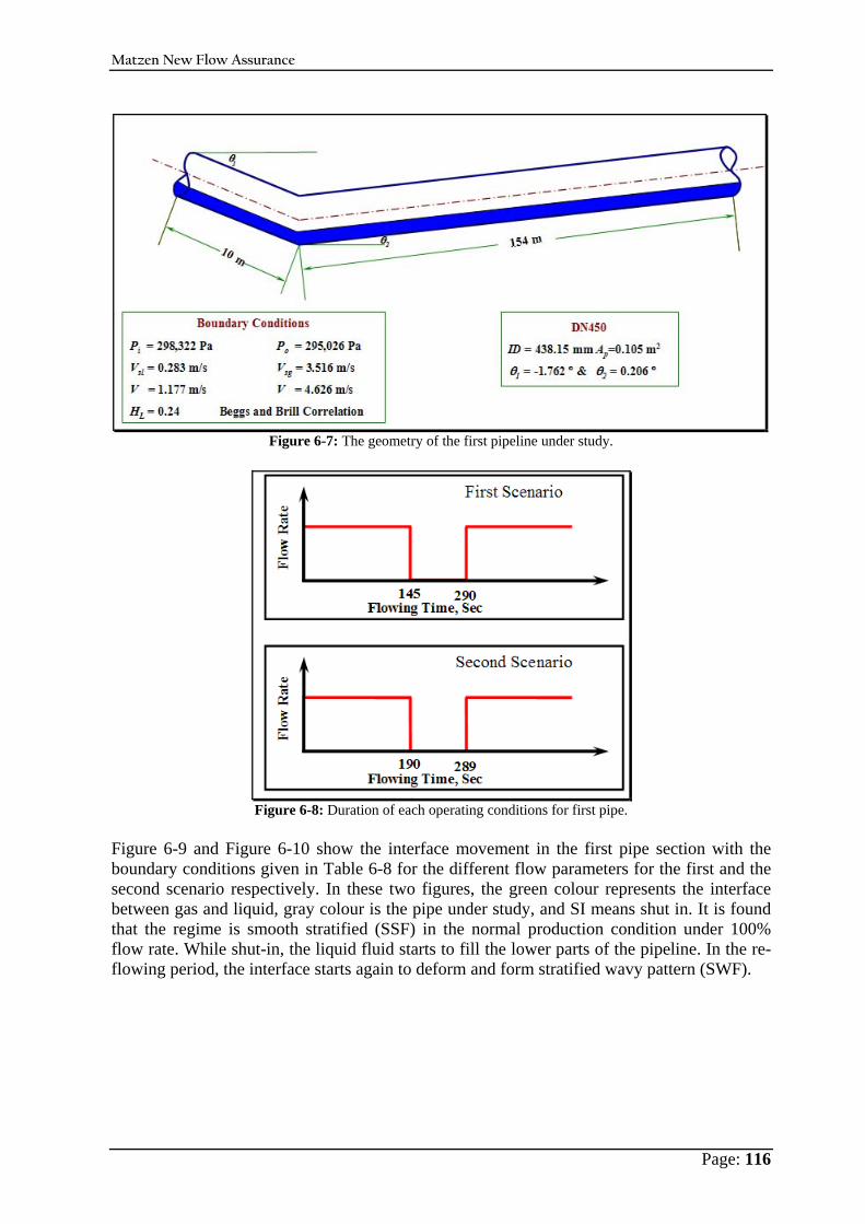
Matzen New Flow Assurance

Page: 116

Figure 6-7: The geometry of the first pipeline under study.

Figure 6-8: Duration of each operating conditions for first pipe.

Figure 6-9 and Figure 6-10 show the interface movement in the first pipe section with the boundary conditions given in Table 6-8 for the different flow parameters for the first and the second scenario respectively. In these two figures, the green colour represents the interface between gas and liquid, gray colour is the pipe under study, and SI means shut in. It is found that the regime is smooth stratified (SSF) in the normal production condition under 100% flow rate. While shut-in, the liquid fluid starts to fill the lower parts of the pipeline. In the re-flowing period, the interface starts again to deform and form stratified wavy pattern (SWF).

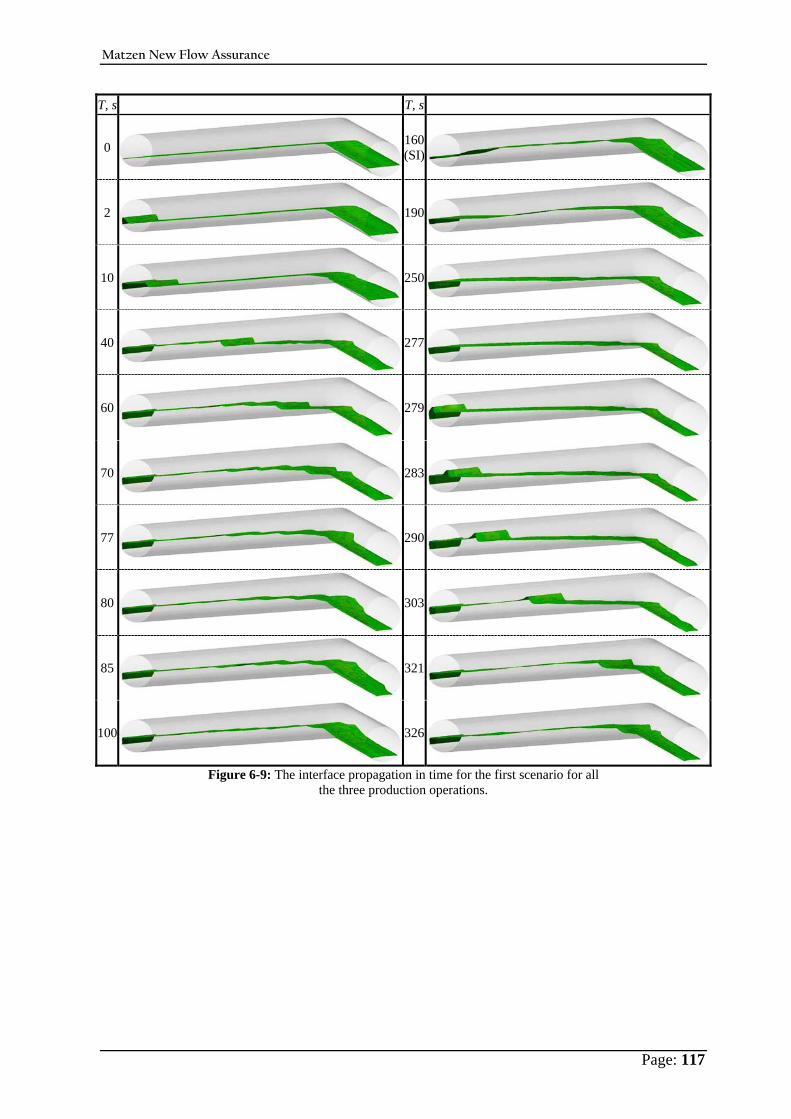
Matzen New Flow Assurance

Page: 117

T, s T, s

0 160(SI)

2 190

10 250

40 277

60 279

70 283

77 290

80 303

85 321

100 326

Figure 6-9: The interface propagation in time for the first scenario for all the three production operations.

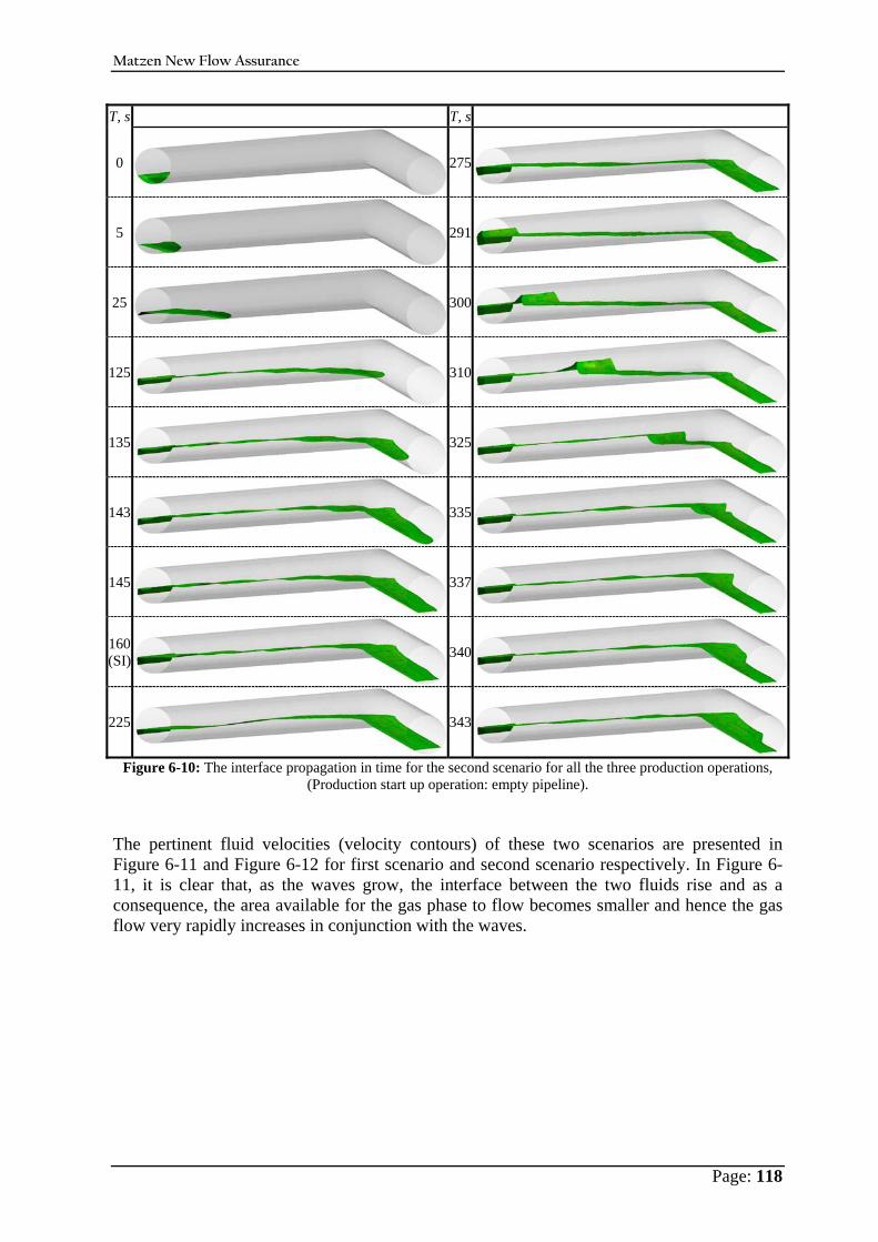
Matzen New Flow Assurance

Page: 118

T, s T, s

0 275

5 291

25 300

125 310

135 325

143 335

145 337

160 (SI) 340

225 343

Figure 6-10: The interface propagation in time for the second scenario for all the three production operations, (Production start up operation: empty pipeline).

The pertinent fluid velocities (velocity contours) of these two scenarios are presented in Figure 6-11 and Figure 6-12 for first scenario and second scenario respectively. In Figure 6-11, it is clear that, as the waves grow, the interface between the two fluids rise and as a consequence, the area available for the gas phase to flow becomes smaller and hence the gas flow very rapidly increases in conjunction with the waves.

Matzen New Flow Assurance

Page: 119

T, s Velocity contour first pipe, first scenario 60

80

10

0 16

0 [S

I Per

iod]

28

0 30

0 32

0

Figure 6-11: Velocity contour of the mixture for the first pipe, first scenario.

Matzen New Flow Assurance

Page: 120

T, s Velocity contour first pipe, second scenario 12

0 14

0 16

0 23

0 [S

I Per

iod]

30

0 32

0 34

0

Figure 6-12: Velocity contour of the mixture for the first pipe, second scenario. Mass flow rate monitoring The liquid mass flow rate versus time for each scenario was monitored at two different positions in each pipe section, one at the joint of the pipeline which is at 110 m, and the second at the outlet of the pipeline, which is illustrated Figure 6-13 in and Figure 6-14 for the first and in Figure 6-15 and Figure 6-16 for the second scenario (start up operation).

Matzen New Flow Assurance

Page: 121

For the first scenario, the figures show that there is a difference in the first 50 s. at the outlet. A peak at 10 s where the big liquid wave reaches the outlet. Afterwards, the rate goes down to empty the liquid existing in the lower part of the pipeline. From then on both of the figures show the same behaviour, react with the incoming waves in a sense the flow stopped at about 145 s, then restarting flow again at about 290 s for the first scenario. These transient effects are very clear in Figure 6-13 and Figure 6-14. Similar observations can be made for the second scenario in a scene that it reacts with the incoming waves as shown in Figure 6-15 and Figure 6-16, except for the first 150 s where no flow at all takes place due to the fact that the liquid does not reach to these two positions yet.

0

10

20

30

40

50

60

0 50 100 150 200 250 300 350 400 450Time, Sec

Mass rate, Kg/Sec

Liquid rate @ 110 m

Figure 6-13: Simulated mass flow rate response for the first pipe, first scenario at 110 m.

0

10

20

30

40

50

60

0 50 100 150 200 250 300 350 400 450Time, Sec

Mass rate, Kg/Sec

Liquid rate @ Outlet

Figure 6-14: Simulated mass flow rate response for the first pipe, first scenario at outlet.

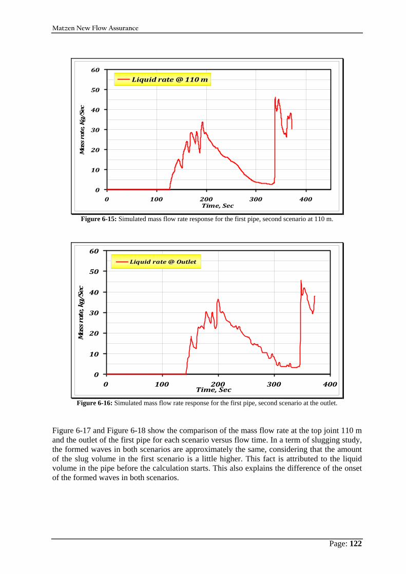
Matzen New Flow Assurance

Page: 122

0

10

20

30

40

50

60

0 100 200 300 400Time, Sec

Mass rate, Kg/Sec

Liquid rate @ 110 m

Figure 6-15: Simulated mass flow rate response for the first pipe, second scenario at 110 m.

0

10

20

30

40

50

60

0 100 200 300 400Time, Sec

Mass rate, kg/Sec

Liquid rate @ Outlet

Figure 6-16: Simulated mass flow rate response for the first pipe, second scenario at the outlet.

Figure 6-17 and Figure 6-18 show the comparison of the mass flow rate at the top joint 110 m and the outlet of the first pipe for each scenario versus flow time. In a term of slugging study, the formed waves in both scenarios are approximately the same, considering that the amount of the slug volume in the first scenario is a little higher. This fact is attributed to the liquid volume in the pipe before the calculation starts. This also explains the difference of the onset of the formed waves in both scenarios.

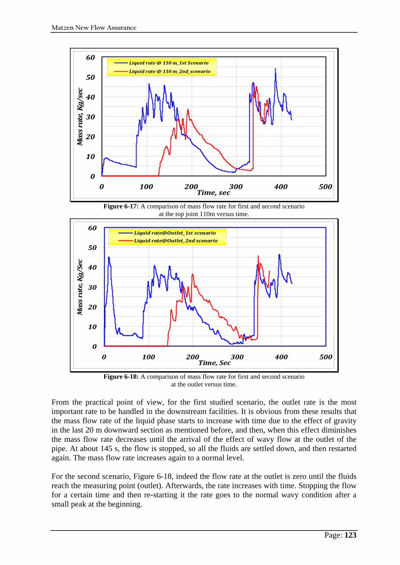
Matzen New Flow Assurance

Page: 123

0

10

20

30

40

50

60

0 100 200 300 400 500Time, sec

Mass rate, Kg/sec

Liquid rate @ 110 m_1st Scenario

Liquid rate @ 110 m_2nd_scenario

Figure 6-17: A comparison of mass flow rate for first and second scenario

at the top joint 110m versus time.

0

10

20

30

40

50

60

0 100 200 300 400 500Time, Sec

Mass rate, Kg/Sec

Liquid rate@Outlet_1st scenario

Liquid rate@Outlet_2nd scenario

Figure 6-18: A comparison of mass flow rate for first and second scenario

at the outlet versus time. From the practical point of view, for the first studied scenario, the outlet rate is the most important rate to be handled in the downstream facilities. It is obvious from these results that the mass flow rate of the liquid phase starts to increase with time due to the effect of gravity in the last 20 m downward section as mentioned before, and then, when this effect diminishes the mass flow rate decreases until the arrival of the effect of wavy flow at the outlet of the pipe. At about 145 s, the flow is stopped, so all the fluids are settled down, and then restarted again. The mass flow rate increases again to a normal level. For the second scenario, Figure 6-18, indeed the flow rate at the outlet is zero until the fluids reach the measuring point (outlet). Afterwards, the rate increases with time. Stopping the flow for a certain time and then re-starting it the rate goes to the normal wavy condition after a small peak at the beginning.

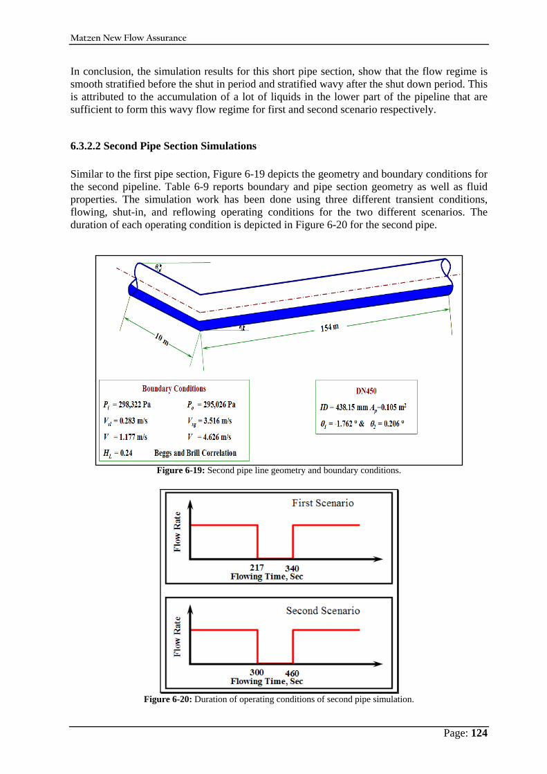
Matzen New Flow Assurance

Page: 124

In conclusion, the simulation results for this short pipe section, show that the flow regime is smooth stratified before the shut in period and stratified wavy after the shut down period. This is attributed to the accumulation of a lot of liquids in the lower part of the pipeline that are sufficient to form this wavy flow regime for first and second scenario respectively.

6.3.2.2 Second Pipe Section Simulations Similar to the first pipe section, Figure 6-19 depicts the geometry and boundary conditions for the second pipeline. Table 6-9 reports boundary and pipe section geometry as well as fluid properties. The simulation work has been done using three different transient conditions, flowing, shut-in, and reflowing operating conditions for the two different scenarios. The duration of each operating condition is depicted in Figure 6-20 for the second pipe.

Figure 6-19: Second pipe line geometry and boundary conditions.

Figure 6-20: Duration of operating conditions of second pipe simulation.

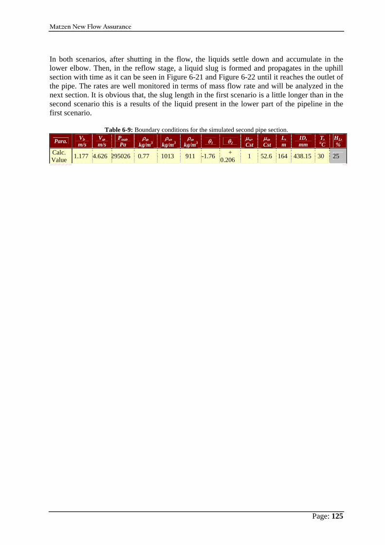
Matzen New Flow Assurance

Page: 125

In both scenarios, after shutting in the flow, the liquids settle down and accumulate in the lower elbow. Then, in the reflow stage, a liquid slug is formed and propagates in the uphill section with time as it can be seen in Figure 6-21 and Figure 6-22 until it reaches the outlet of the pipe. The rates are well monitored in terms of mass flow rate and will be analyzed in the next section. It is obvious that, the slug length in the first scenario is a little longer than in the second scenario this is a results of the liquid present in the lower part of the pipeline in the first scenario.

Table 6-9: Boundary conditions for the simulated second pipe section.

Para. Vl, m/s

Vg, m/s

Pout, Pa

ρg, kg/m3

ρw, kg/m3

ρo, kg/m3 θ1 θ2

μw. Cst

μo, Cst

L, m

ID, mm

T, oC

HL, %

Calc. Value 1.177 4.626 295026 0.77 1013 911 -1.76 +

0.206 1 52.6 164 438.15 30 25

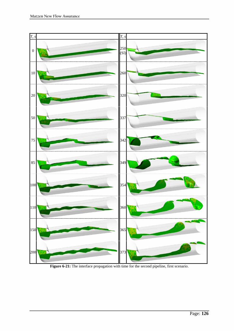
Matzen New Flow Assurance

Page: 126

T, s T, s

0 250(SI)

10 260

20 320

50 337

75 342

85 349

100 354

110 360

150 365

200 373

Figure 6-21: The interface propagation with time for the second pipeline, first scenario.

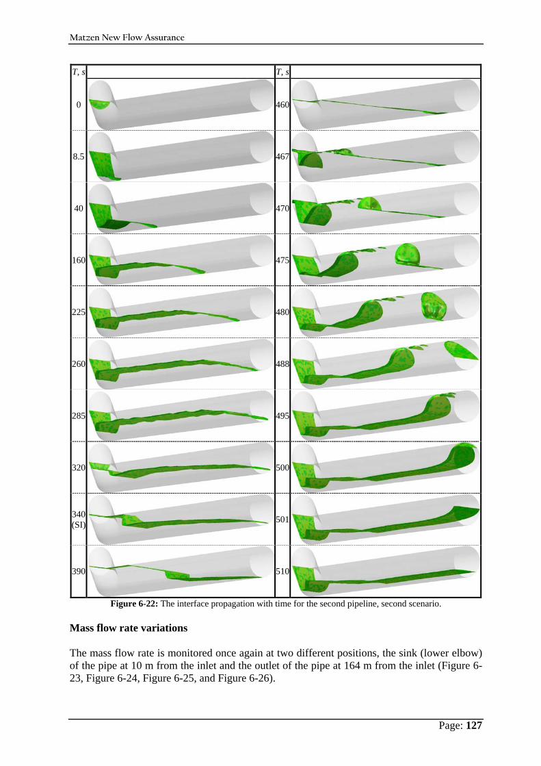
Matzen New Flow Assurance

Page: 127

T, s T, s

0 460

8.5 467

40 470

160 475

225 480

260 488

285 495

320 500

340 (SI) 501

390 510

Figure 6-22: The interface propagation with time for the second pipeline, second scenario. Mass flow rate variations The mass flow rate is monitored once again at two different positions, the sink (lower elbow) of the pipe at 10 m from the inlet and the outlet of the pipe at 164 m from the inlet (Figure 6-23, Figure 6-24, Figure 6-25, and Figure 6-26).

Matzen New Flow Assurance

Page: 128

0

100

200

300

400

500

600

0 50 100 150 200 250 300 350 400Time, Sec

Mass rate, kg/Sec

Liquid rate@ 10m

Figure 6-23: Simulated mass flow rate response for the second pipe, first scenario at 10 m.

In Figure 6-23, the flow rate is increased with time until the first 7 s. As a result of gravity effects the rate diminishes gradually with time, until normal conditions. There is no rate at all in the shut-in period, the fluids are stagnant. Afterwards, a big slug is formed and passes very fast. At the end, the rate returned to the normal rate. At the outlet, the rate increases in the first few seconds then decreases to zero because the fluid must fill the pipe elbow first. After increasing again at about 140 s, the interface varies due to fluctuations until going to zero at about 290 s once again. The formed slug reaches the outlet at about 360 s with a very large amount for about 20 s.

0

100

200

300

400

500

600

0 50 100 150 200 250 300 350 400Time, Sec

Mass rate, kg/Sec

Liquid rate@ Outlet

Figure 6-24: Simulated mass flow rate response for the second pipe, first scenario at outlet.

Figure 6-26 depicts the situation for the second scenario, the mass flow rate at 10 m is the same like for the first scenario except for the first 10 s, this is due to the fact that the pipe is

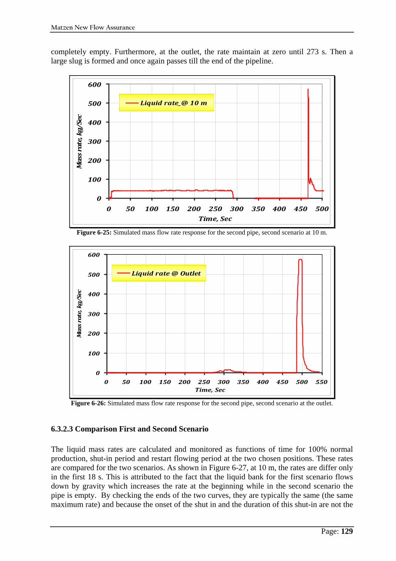
Matzen New Flow Assurance

Page: 129

completely empty. Furthermore, at the outlet, the rate maintain at zero until 273 s. Then a large slug is formed and once again passes till the end of the pipeline.

0

100

200

300

400

500

600

0 50 100 150 200 250 300 350 400 450 500Time, Sec

Mass rate, kg/Sec 

Liquid rate_@ 10 m

Figure 6-25: Simulated mass flow rate response for the second pipe, second scenario at 10 m.

0

100

200

300

400

500

600

0 50 100 150 200 250 300 350 400 450 500 550Time, Sec

Mass rate, kg/Sec

Liquid rate @ Outlet

Figure 6-26: Simulated mass flow rate response for the second pipe, second scenario at the outlet.

6.3.2.3 Comparison First and Second Scenario The liquid mass rates are calculated and monitored as functions of time for 100% normal production, shut-in period and restart flowing period at the two chosen positions. These rates are compared for the two scenarios. As shown in Figure 6-27, at 10 m, the rates are differ only in the first 18 s. This is attributed to the fact that the liquid bank for the first scenario flows down by gravity which increases the rate at the beginning while in the second scenario the pipe is empty. By checking the ends of the two curves, they are typically the same (the same maximum rate) and because the onset of the shut in and the duration of this shut-in are not the

Matzen New Flow Assurance

Page: 130

same in the scenarios, they are not overlapped. It is observed that the rate after reflowing is exactly the same as before. As a comparison between first and second scenario, it can be seen in Figure 6-28, that slug length and volume are approximately the same.

0

100

200

300

400

500

600

0 50 100 150 200 250 300 350 400 450 500 550

Time, Sec

Mass rate, Kg/Sec

Liquid rate@ 10 m_1st ScenarioLiquid rate@ 10 m_2nd Scenario

Figure 6-27: Simulated mass flow rate variations for the second pipe at 10 m.

0

100

200

300

400

500

600

700

0 100 200 300 400 500 600Time, Sec

Mass rate, Kg/Sec

Liquid rate@ Outlet_1st ScenarioLiquid rate @ Outlet_2nd Scenario

Figure 6-28: Simulated mass flow rate variations for the second pipe at outlet.

Similar to the analysis of the first pipe section, velocity contours are displayed in Figure 6-29 and Figure 6-30 for the second pipe section first scenario and second scenario respectively.

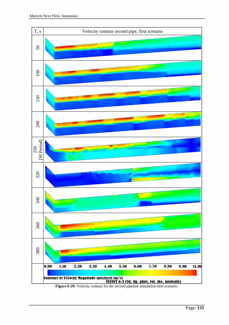
Matzen New Flow Assurance

Page: 131

T, s Velocity contour second pipe, first scenario 50

10

0 15

0 20

0 25

0 [S

I Per

iod]

32

0 34

0 36

0 38

0

Figure 6-29: Velocity contour for the second pipeline simulation-first scenario.

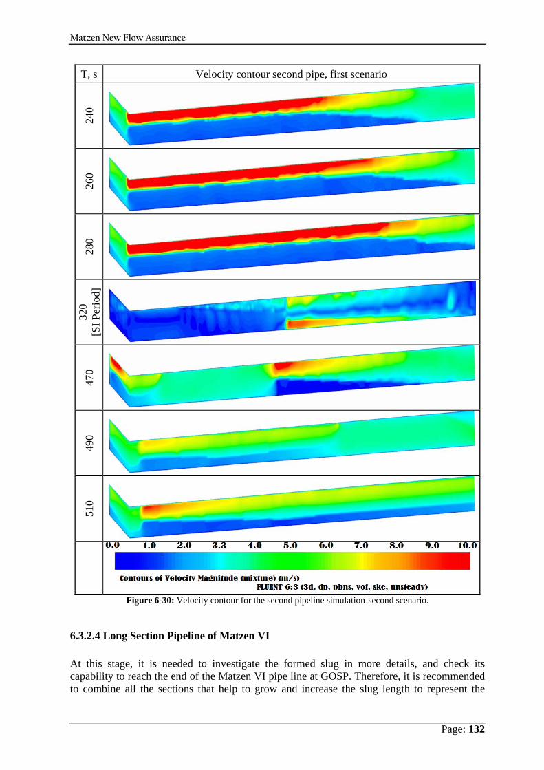
Matzen New Flow Assurance

Page: 132

T, s Velocity contour second pipe, first scenario 24

0 26

0 28

0 32

0 [S

I Per

iod]

47

0 49

0 51

0

Figure 6-30: Velocity contour for the second pipeline simulation-second scenario.

6.3.2.4 Long Section Pipeline of Matzen VI At this stage, it is needed to investigate the formed slug in more details, and check its capability to reach the end of the Matzen VI pipe line at GOSP. Therefore, it is recommended to combine all the sections that help to grow and increase the slug length to represent the

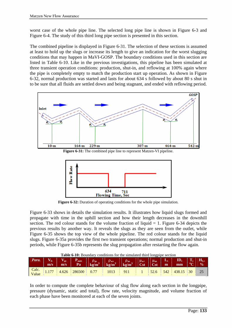
Matzen New Flow Assurance

Page: 133

worst case of the whole pipe line. The selected long pipe line is shown in Figure 6-3 and Figure 6-4. The study of this third long pipe section is presented in this section. The combined pipeline is displayed in Figure 6-31. The selection of these sections is assumed at least to hold up the slugs or increase its length to give an indication for the worst slugging conditions that may happen in MaVI-GOSP. The boundary conditions used in this section are listed in Table 6-10. Like in the previous investigations, this pipeline has been simulated at three transient operation conditions: production, shut-in, and reflowing at 100% again where the pipe is completely empty to match the production start up operation. As shown in Figure 6-32, normal production was started and lasts for about 634 s followed by about 80 s shut in to be sure that all fluids are settled down and being stagnant, and ended with reflowing period.

Figure 6-31: The combined pipe line to represent Matzen-VI pipeline.

Figure 6-32: Duration of operating conditions for the whole pipe simulation.

Figure 6-33 shows in details the simulation results. It illustrates how liquid slugs formed and propagate with time in the uphill section and how their length decreases in the downhill section. The red colour stands for the volume fraction of liquid = 1. Figure 6-34 depicts the previous results by another way. It reveals the slugs as they are seen from the outlet, while Figure 6-35 shows the top view of the whole pipeline. The red colour stands for the liquid slugs. Figure 6-35a provides the first two transient operations; normal production and shut-in periods, while Figure 6-35b represents the slug propagation after restarting the flow again.

Table 6-10: Boundary conditions for the simulated third longpipe section Para. Vl,

m/s Vg, m/s

Pout, Pa

ρg, kg/m3

ρw, kg/m3

ρo, kg/m3

μw. Cst

μo, Cst

L, m

ID, mm

T, oC

HL, %

Calc. Value 1.177 4.626 286500 0.77 1013 911 1 52.6 542 438.15 30 25

In order to compute the complete behaviour of slug flow along each section in the longpipe, pressure (dynamic, static and total), flow rate, velocity magnitude, and volume fraction of each phase have been monitored at each of the seven joints.

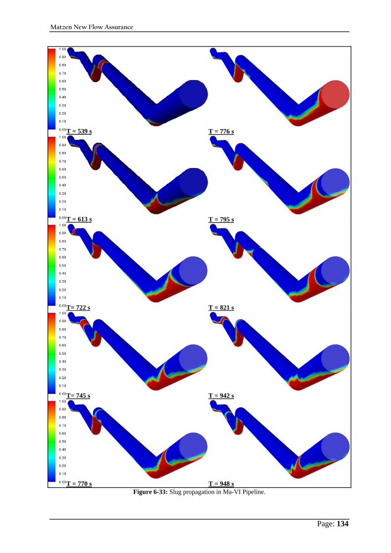
Matzen New Flow Assurance

Page: 134

T = 539 s T = 776 s

T = 613 s T = 795 s

T= 722 s T = 821 s

T= 745 s T = 942 s

T = 770 s T = 948 s Figure 6-33: Slug propagation in Ma-VI Pipeline.

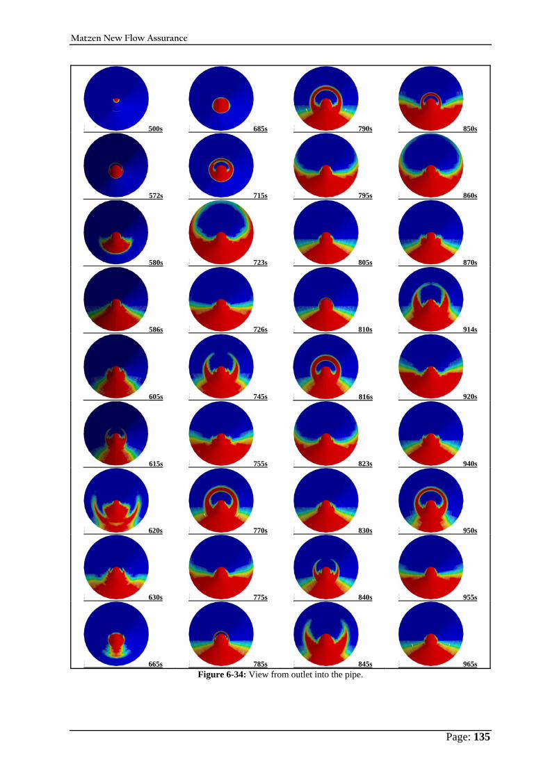
Matzen New Flow Assurance

Page: 135

500s 685s 790s 850s

572s 715s 795s 860s

580s 723s 805s 870s

586s 726s 810s 914s

605s 745s 816s 920s

615s 755s 823s 940s

620s 770s 830s 950s

630s 775s 840s 955s

665s 785s 845s 965s Figure 6-34: View from outlet into the pipe.

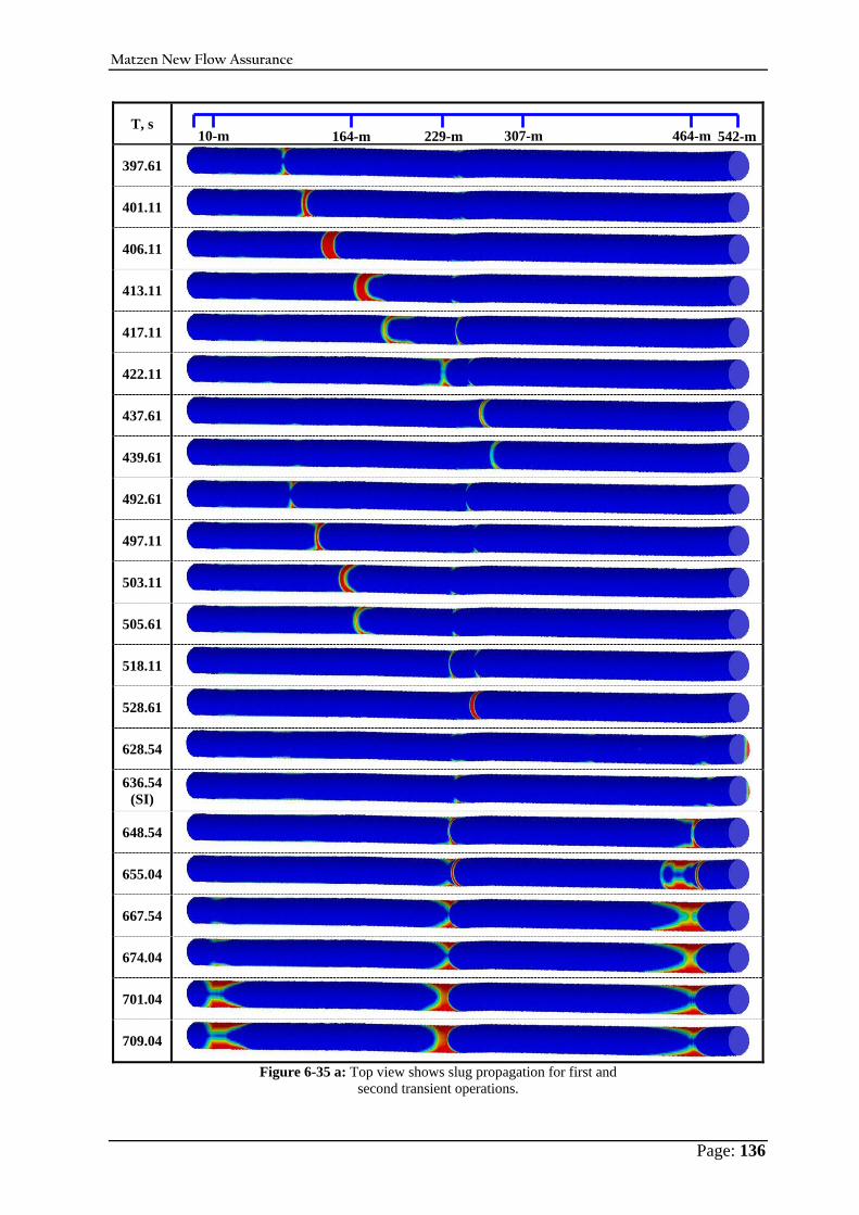
Matzen New Flow Assurance

Page: 136

T, s

397.61

401.11

406.11

413.11

417.11

422.11

437.61

439.61

492.61

497.11

503.11

505.61

518.11

528.61

628.54

636.54 (SI)

648.54

655.04

667.54

674.04

701.04

709.04

Figure 6-35 a: Top view shows slug propagation for first and second transient operations.

10-m 164-m 229-m 307-m 464-m 542-m

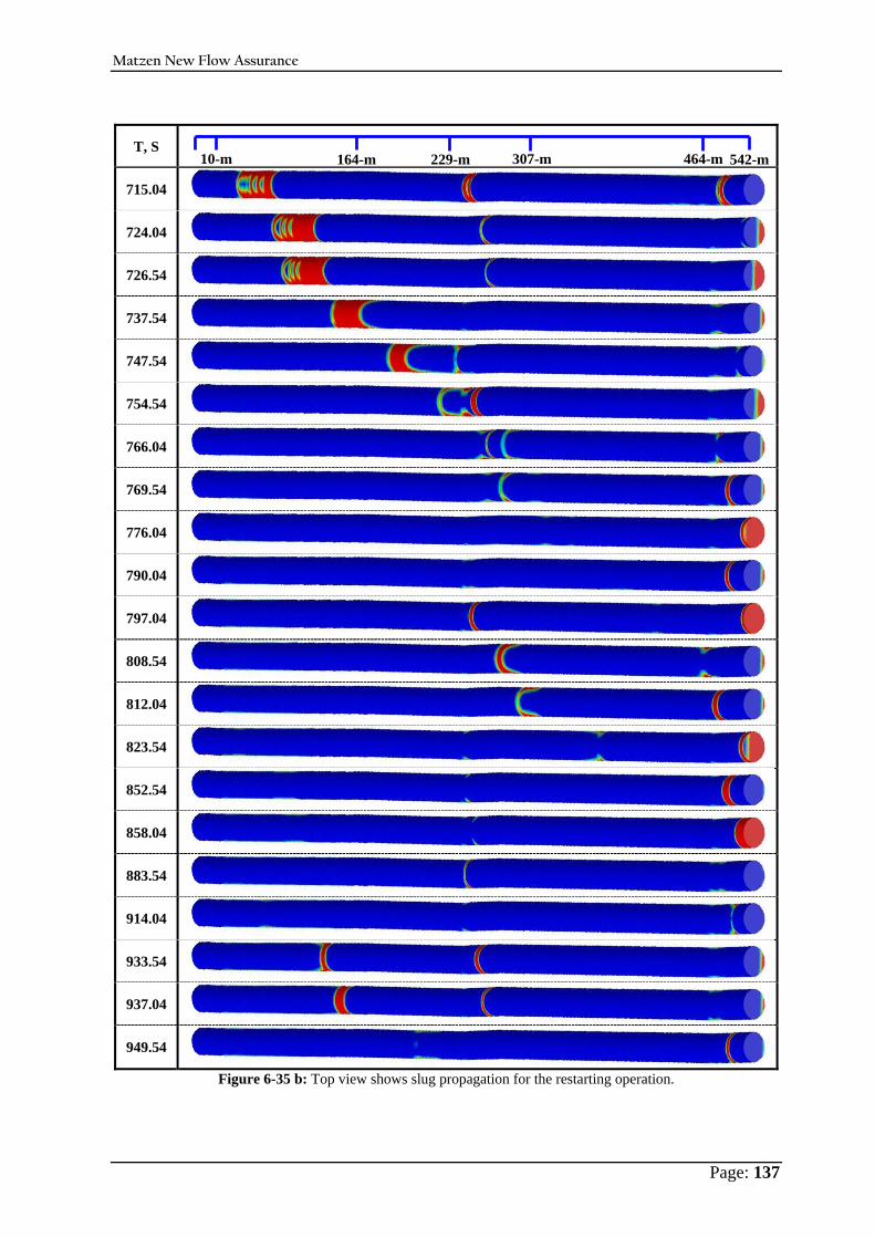
Matzen New Flow Assurance

Page: 137

T, S

715.04

724.04

726.54

737.54

747.54

754.54

766.04

769.54

776.04

790.04

797.04

808.54

812.04

823.54

852.54

858.04

883.54

914.04

933.54

937.04

949.54

Figure 6-35 b: Top view shows slug propagation for the restarting operation.

10-m 164-m 229-m 307-m 464-m 542-m

Matzen New Flow Assurance

Page: 138

6.3.2.3.1 Liquid Holdup A complete monitoring of the volume fraction of each phase has been done at each joint of long-pipe Matzen VI, i. e. at 10, 164, 229, 307, 464, and 542m. It was found that, the distribution behaviour of the liquid holdup with time at each section is not the same. This is attributed to the geometry and the topology of the pipeline in addition to the changes due to flow regimes. It is also observed that the liquid holdup for the lower elbows is completely different from that at the upper elbows. Figure 6-36 shows this fact by representing the total volume fraction monitored at these locations. It is noted that the volume fraction variations at the sink points (lower elbows at 10, 229 and 464 m) are not showing the same trend as for the upper elbows (164, 307 and 542 m). In the lower elbow, there are very big fluctuations at each sink point. Furthermore, as the figure shows, the liquid holdup along the pipe is not constant with time. Moreover, by checking all liquid holdup behaviour in each section, it is found that the complete slug unit formed in an upward section dissipates completely in the next downward section. The last pipe section in MaVI-GOSP is an upward section and therefore, the formed slug reaches the end of the pipe at main separation station GOSP. Figure 6-36b, Figure 6-36d, and Figure 6-36f display that the flow pattern in the pipeline is a slug flow and that the slug length increase with time within the studied period. This behaviour is also documented in the literature[ 6-25] and called “slug growth”. Practically, it is important to have complete information about the slugging characteristics for the slugs that are able to reach the separation station GOSP in order to be handled, and this will be given in details in the following sections.

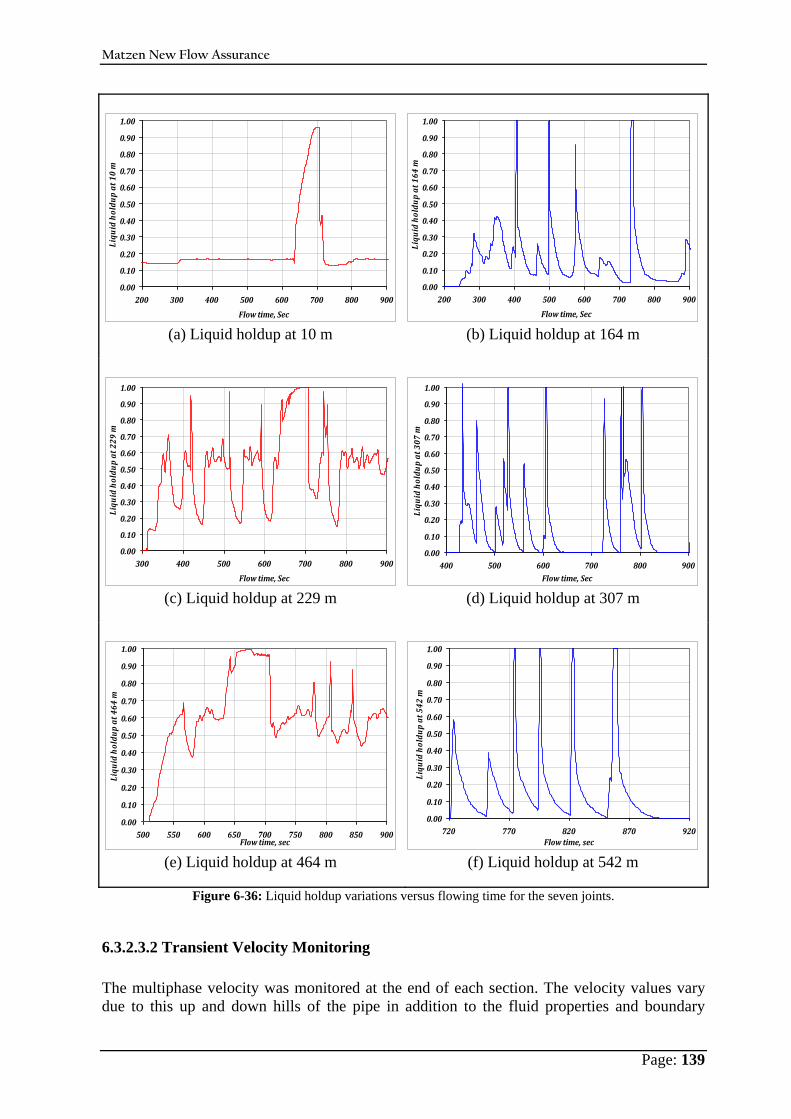
Matzen New Flow Assurance

Page: 139

0.00

0.10

0.20

0.30

0.40

0.50

0.60

0.70

0.80

0.90

1.00

200 300 400 500 600 700 800 900

Flow time, Sec

Liquid holdup at 10 m

(a) Liquid holdup at 10 m

0.00

0.10

0.20

0.30

0.40

0.50

0.60

0.70

0.80

0.90

1.00

200 300 400 500 600 700 800 900

Flow time, Sec

Liquid holdup at 164 m

(b) Liquid holdup at 164 m

0.00

0.10

0.20

0.30

0.40

0.50

0.60

0.70

0.80

0.90

1.00

300 400 500 600 700 800 900

Flow time, Sec

Liquid holdup at 229 m

(c) Liquid holdup at 229 m

0.00

0.10

0.20

0.30

0.40

0.50

0.60

0.70

0.80

0.90

1.00

400 500 600 700 800 900Flow time, Sec

Liquid holdup at 307 m

(d) Liquid holdup at 307 m

0.00

0.10

0.20

0.30

0.40

0.50

0.60

0.70

0.80

0.90

1.00

500 550 600 650 700 750 800 850 900Flow time, sec

Liquid holdup at 464 m

(e) Liquid holdup at 464 m

0.00

0.10

0.20

0.30

0.40

0.50

0.60

0.70

0.80

0.90

1.00

720 770 820 870 920Flow time, sec

Liquid holdup at 542 m

(f) Liquid holdup at 542 m

Figure 6-36: Liquid holdup variations versus flowing time for the seven joints.

6.3.2.3.2 Transient Velocity Monitoring The multiphase velocity was monitored at the end of each section. The velocity values vary due to this up and down hills of the pipe in addition to the fluid properties and boundary

Matzen New Flow Assurance

Page: 140

conditions. Figure 6-37 represents these variations at all joints of the studied pipeline at 10, 164, 229, 307, 464 and 542 respectively. In all of these figures, the velocity goes to zero in the shut down period. In the sink positions at 229 and 464, the fluctuation is clear which represents the interface movements. In upper elbows, the fluctuation is more translated as in Figure 6-37d and Figure 6-37f. The velocity variation at 229 m ranges from 3.8 to 4 m/s and therefore, fluctuates more than at 542 m section (3.8 to 3.86 m/s). The reason for these larger variations is the change of flow direction. At 229 m, the fluid flows downwards with a higher velocity then in the redirected upward flow.

3.75

3.77

3.79

3.81

3.83

3.85

100 200 300 400 500 600 700 800 900Flow time, m/sec

Velocity mag. m

/sec @

 10 m

(a) Velocity magnitude at 10 m

3.75

3.77

3.79

3.81

3.83

3.85

200 300 400 500 600 700 800 900Flow time, m/sec

Velocity mag. m

/sec @

 164

 m

(b) Velocity magnitude at 164 m

3.70

3.75

3.80

3.85

3.90

3.95

4.00

4.05

4.10

300 400 500 600 700 800 900Flow time, m/sec

Velocity mag. m

/sec @

 229

 m

(c) Velocity magnitude at 229 m

3.75

3.77

3.79

3.81

3.83

3.85

3.87

3.89

400 500 600 700 800 900

Flow Time, sec

Velocity Mag., m/sec @ 307 m

(d) Velocity magnitude at 307 m

3.75

3.77

3.79

3.81

3.83

3.85

3.87

3.89

500 600 700 800 900

Flow Time, sec

Velocity Mag., m/sec @ 464 m

(e) Velocity magnitude at 464 m

3.790

3.795

3.800

3.805

3.810

3.815

3.820

550 600 650 700 750 800 850 900

Flow Time, Sec

Velocity, m/sec @ 542 m

(f) Velocity magnitude at 542 m Figure 6-37: Velocity magnitude versus time for multiphase flow on Matzen VI.

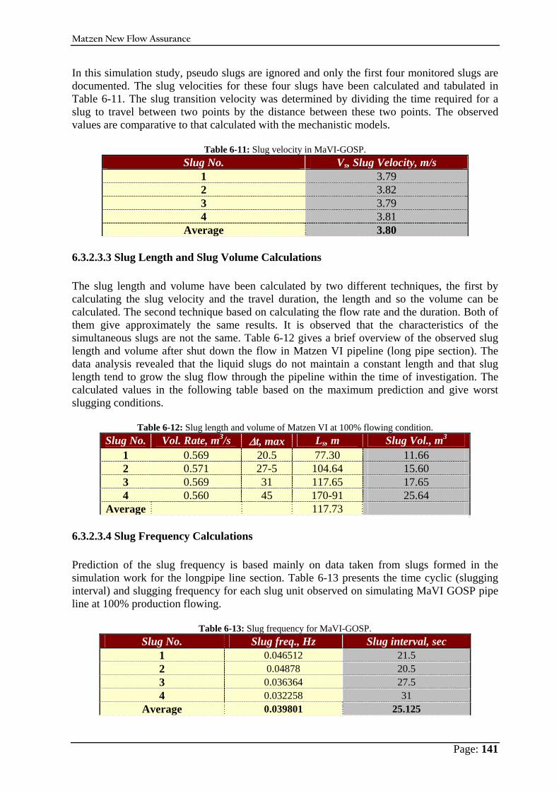
Matzen New Flow Assurance

Page: 141

In this simulation study, pseudo slugs are ignored and only the first four monitored slugs are documented. The slug velocities for these four slugs have been calculated and tabulated in Table 6-11. The slug transition velocity was determined by dividing the time required for a slug to travel between two points by the distance between these two points. The observed values are comparative to that calculated with the mechanistic models.

Table 6-11: Slug velocity in MaVI-GOSP. Slug No. Vs, Slug Velocity, m/s

1 3.79 2 3.82 3 3.79 4 3.81

Average 3.80

6.3.2.3.3 Slug Length and Slug Volume Calculations The slug length and volume have been calculated by two different techniques, the first by calculating the slug velocity and the travel duration, the length and so the volume can be calculated. The second technique based on calculating the flow rate and the duration. Both of them give approximately the same results. It is observed that the characteristics of the simultaneous slugs are not the same. Table 6-12 gives a brief overview of the observed slug length and volume after shut down the flow in Matzen VI pipeline (long pipe section). The data analysis revealed that the liquid slugs do not maintain a constant length and that slug length tend to grow the slug flow through the pipeline within the time of investigation. The calculated values in the following table based on the maximum prediction and give worst slugging conditions.

Table 6-12: Slug length and volume of Matzen VI at 100% flowing condition. Slug No. Vol. Rate, m3/s Δt, max Ls, m Slug Vol., m3

1 0.569 20.5 77.30 11.66 2 0.571 27-5 104.64 15.60 3 0.569 31 117.65 17.65 4 0.560 45 170-91 25.64

Average 117.73

6.3.2.3.4 Slug Frequency Calculations Prediction of the slug frequency is based mainly on data taken from slugs formed in the simulation work for the longpipe line section. Table 6-13 presents the time cyclic (slugging interval) and slugging frequency for each slug unit observed on simulating MaVI GOSP pipe line at 100% production flowing.

Table 6-13: Slug frequency for MaVI-GOSP. Slug No. Slug freq., Hz Slug interval, sec

1 0.046512 21.5 2 0.04878 20.5 3 0.036364 27.5 4 0.032258 31

Average 0.039801 25.125

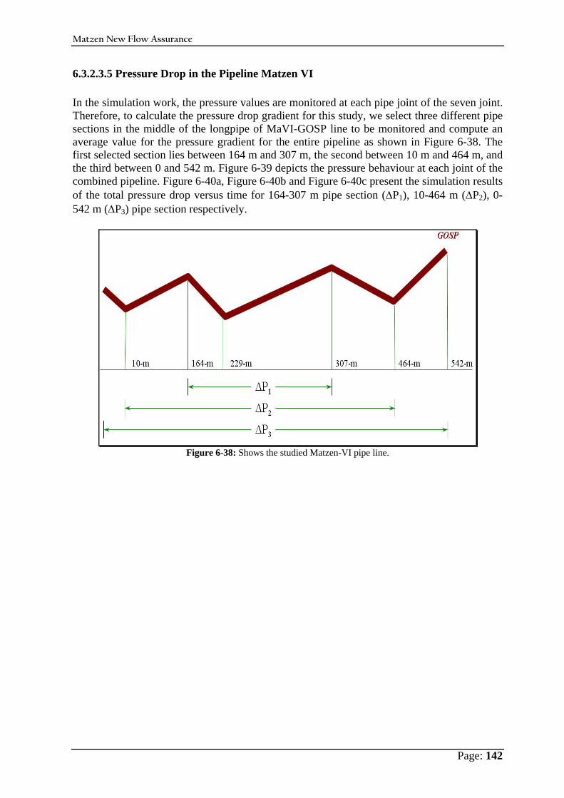
Matzen New Flow Assurance

Page: 142

6.3.2.3.5 Pressure Drop in the Pipeline Matzen VI In the simulation work, the pressure values are monitored at each pipe joint of the seven joint. Therefore, to calculate the pressure drop gradient for this study, we select three different pipe sections in the middle of the longpipe of MaVI-GOSP line to be monitored and compute an average value for the pressure gradient for the entire pipeline as shown in Figure 6-38. The first selected section lies between 164 m and 307 m, the second between 10 m and 464 m, and the third between 0 and 542 m. Figure 6-39 depicts the pressure behaviour at each joint of the combined pipeline. Figure 6-40a, Figure 6-40b and Figure 6-40c present the simulation results of the total pressure drop versus time for 164-307 m pipe section (ΔP1), 10-464 m (ΔP2), 0-542 m (ΔP3) pipe section respectively.

Figure 6-38: Shows the studied Matzen-VI pipe line.

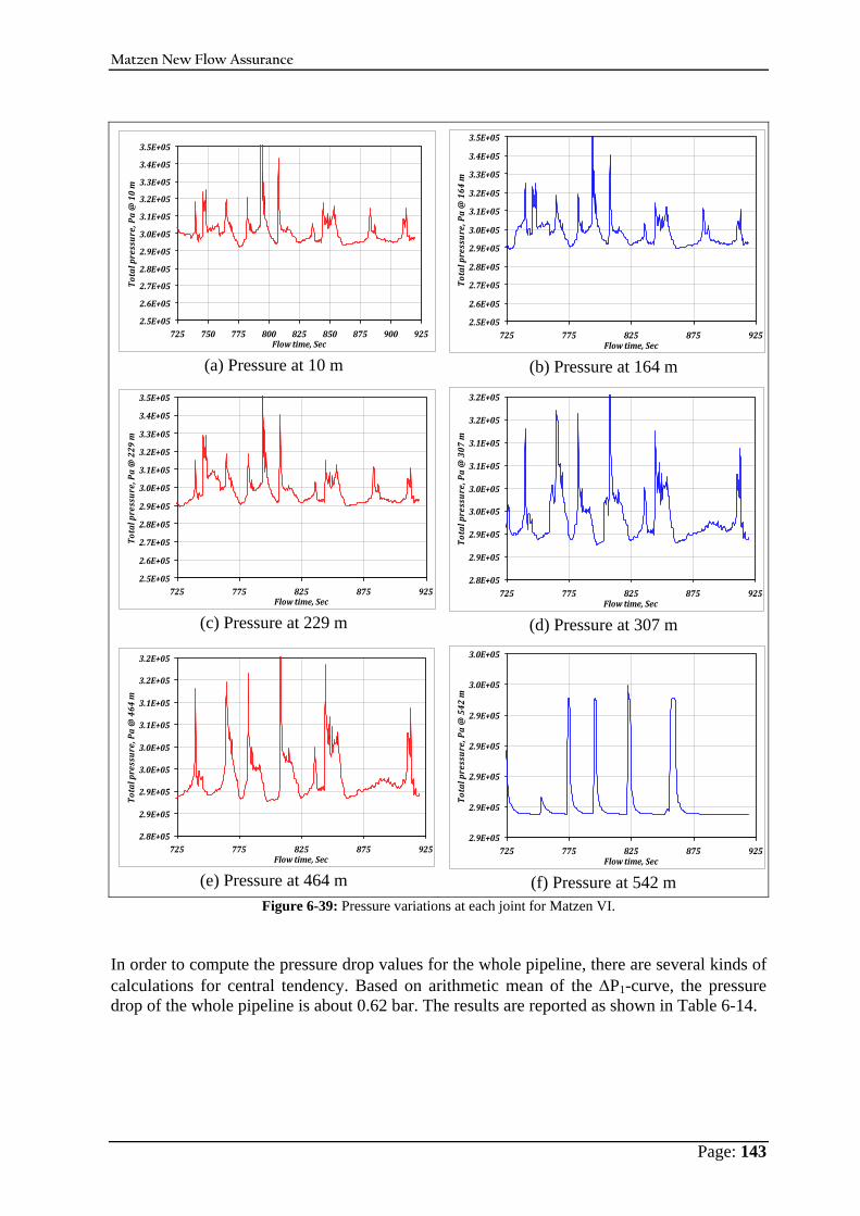
Matzen New Flow Assurance

Page: 143

2.5E+05

2.6E+05

2.7E+05

2.8E+05

2.9E+05

3.0E+05

3.1E+05

3.2E+05

3.3E+05

3.4E+05

3.5E+05

725 750 775 800 825 850 875 900 925Flow time, Sec

Total pressure, Pa @ 10 m

(a) Pressure at 10 m

2.5E+05

2.6E+05

2.7E+05

2.8E+05

2.9E+05

3.0E+05

3.1E+05

3.2E+05

3.3E+05

3.4E+05

3.5E+05

725 775 825 875 925Flow time, Sec

Total pressure, Pa @ 164 m

(b) Pressure at 164 m

2.5E+05

2.6E+05

2.7E+05

2.8E+05

2.9E+05

3.0E+05

3.1E+05

3.2E+05

3.3E+05

3.4E+05

3.5E+05

725 775 825 875 925Flow time, Sec

Total pressure, Pa @ 229 m

(c) Pressure at 229 m

2.8E+05

2.9E+05

2.9E+05

3.0E+05

3.0E+05

3.1E+05

3.1E+05

3.2E+05

3.2E+05

725 775 825 875 925Flow time, Sec

Total pressure, Pa @ 307 m

(d) Pressure at 307 m

2.8E+05

2.9E+05

2.9E+05

3.0E+05

3.0E+05

3.1E+05

3.1E+05

3.2E+05

3.2E+05

725 775 825 875 925Flow time, Sec

Total pressure, Pa @ 464 m

(e) Pressure at 464 m

2.9E+05

2.9E+05

2.9E+05

2.9E+05

2.9E+05

3.0E+05

3.0E+05

725 775 825 875 925Flow time, Sec

Total pressure, Pa @ 542 m

(f) Pressure at 542 m Figure 6-39: Pressure variations at each joint for Matzen VI.

In order to compute the pressure drop values for the whole pipeline, there are several kinds of calculations for central tendency. Based on arithmetic mean of the ΔP1-curve, the pressure drop of the whole pipeline is about 0.62 bar. The results are reported as shown in Table 6-14.

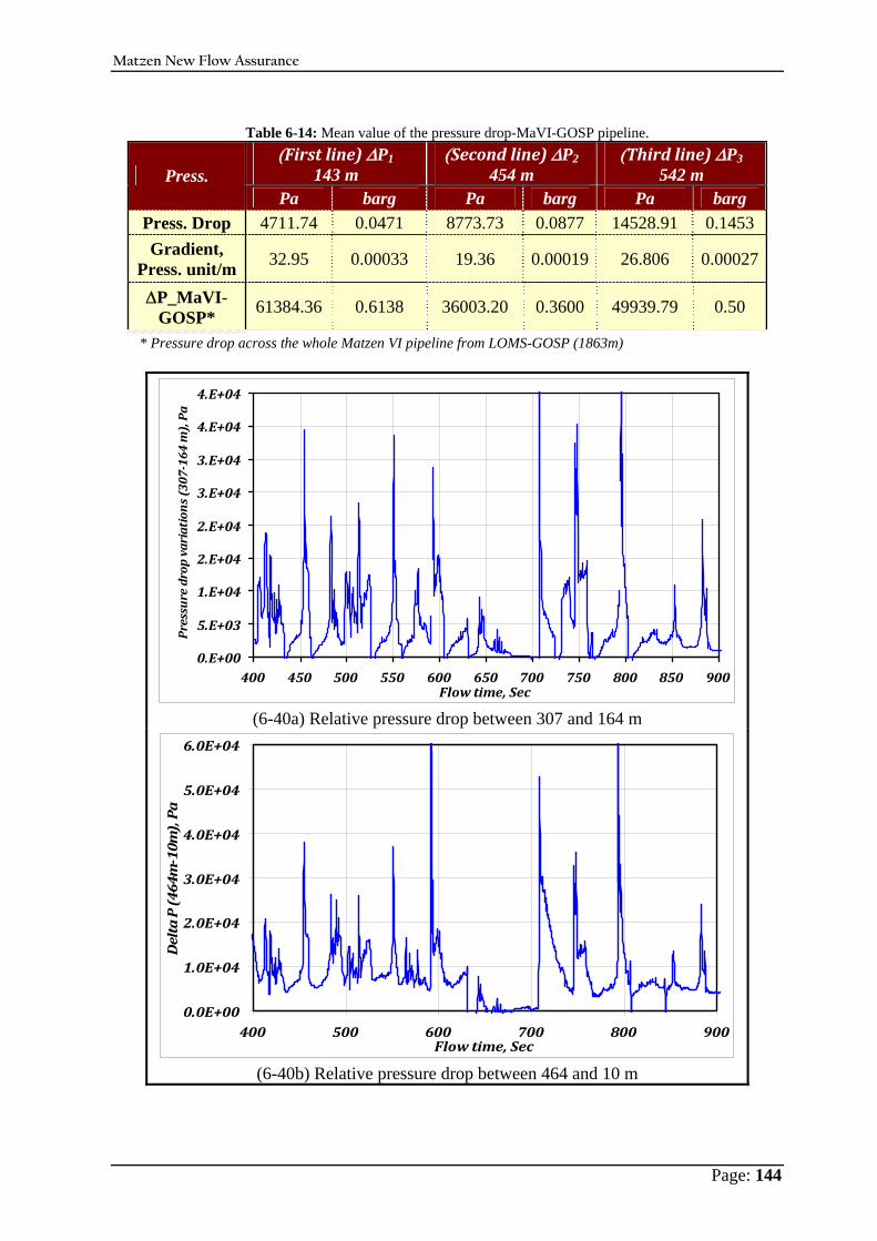
Matzen New Flow Assurance

Page: 144

Table 6-14: Mean value of the pressure drop-MaVI-GOSP pipeline.

(First line) ΔP1 143 m

(Second line) ΔP2 454 m

(Third line) ΔP3 542 m Press.

Pa barg Pa barg Pa barg Press. Drop 4711.74 0.0471 8773.73 0.0877 14528.91 0.1453 Gradient,

Press. unit/m 32.95 0.00033 19.36 0.00019 26.806 0.00027

ΔP_MaVI-GOSP*

61384.36 0.6138 36003.20 0.3600 49939.79 0.50

* Pressure drop across the whole Matzen VI pipeline from LOMS-GOSP (1863m)

0.E+00

5.E+03

1.E+04

2.E+04

2.E+04

3.E+04

3.E+04

4.E+04

4.E+04

400 450 500 550 600 650 700 750 800 850 900Flow time, Sec

Pressure drop variations (307­164 m), Pa  

(6-40a) Relative pressure drop between 307 and 164 m

0.0E+00

1.0E+04

2.0E+04

3.0E+04

4.0E+04

5.0E+04

6.0E+04

400 500 600 700 800 900Flow time, Sec

Delta P (464m

­10m), Pa

(6-40b) Relative pressure drop between 464 and 10 m

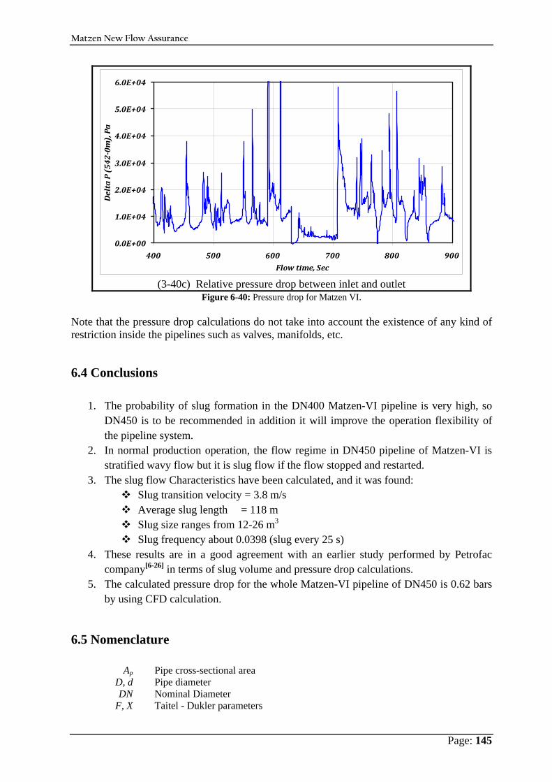
Matzen New Flow Assurance

Page: 145

0.0E+00

1.0E+04

2.0E+04

3.0E+04

4.0E+04

5.0E+04

6.0E+04

400 500 600 700 800 900

Flow time, Sec

Delta P (542­0m

), Pa

(3-40c) Relative pressure drop between inlet and outlet Figure 6-40: Pressure drop for Matzen VI.

Note that the pressure drop calculations do not take into account the existence of any kind of restriction inside the pipelines such as valves, manifolds, etc.

6.4 Conclusions 1. The probability of slug formation in the DN400 Matzen-VI pipeline is very high, so

DN450 is to be recommended in addition it will improve the operation flexibility of the pipeline system.

2. In normal production operation, the flow regime in DN450 pipeline of Matzen-VI is stratified wavy flow but it is slug flow if the flow stopped and restarted.

3. The slug flow Characteristics have been calculated, and it was found: Slug transition velocity = 3.8 m/s Average slug length = 118 m Slug size ranges from 12-26 m3 Slug frequency about 0.0398 (slug every 25 s)

4. These results are in a good agreement with an earlier study performed by Petrofac company[ 6-26] in terms of slug volume and pressure drop calculations.

5. The calculated pressure drop for the whole Matzen-VI pipeline of DN450 is 0.62 bars by using CFD calculation.

6.5 Nomenclature

Ap Pipe cross-sectional area D, d Pipe diameter DN Nominal Diameter

F, X Taitel - Dukler parameters

Matzen New Flow Assurance

Page: 146

Fs Slug frequency HL Liquid holdup ID Internal diameter L Pipe line length

Ls Slug length NFR Froude number

P Pressure Pi Inlet pressure

Pout, Po Outlet pressure T Temperature

Vg True gas velocity Vl True liquid velocity

Vm Mixture velocity Vs, Vts Slug transient velocity

Vsg Superficial gas velocity Vsl Superficial liquid velocity λ In-put liquid volume fraction θi inclination angle

μo, μw Oil and water viscosity ρo, ρw , ρg Oil , water, and gas density

ΔP Pressure drop Δt Time duration

6.6 References

6-1. Data obtained from OMV, 30 Nov. 2006. 6-2. Beggs, H. D. and Brill, J. P.: “A Study of Two-Phase Flow in Inclined Pipes,” JPT,

Vol. 25, No. 5, Pages 607-617, May 1973. 6-3. Weisman, J., Duncan, D., Gibson, J. and Crawford, T.: “Effects of Fluid Properties

and Pipe Diameter on Two-Phase Flow Patterns in Horizontal Lines,” International Journal of Multiphase Flow, Vol. 5, No. 1, Pages 437-462, 1979.

6-4. Mandhane, J. M., Gregory, G. A. and Aziz, K.: “Critical Evaluation of Holdup Prediction Methods for Gas-Liquid Flow in Horizontal Pipes,” SPE 5140 & JPT, Vol. 27, Pages 1017-1026, August 1975.

6-5. Taitel Y. and Dukler A. E.: “A Model for Prediction Flow Regime Transitions in Horizontal and Near Horizontal Gas-Liquid Flow,” AIChE J., Vol. 22, Issue 5, Pages 47-55, Jan. 1976.

6-6. Petalas N. and Aziz, K. : “A Mechanistic Model For Multiphase Flow in Pipe,” Paper no. 98-39, Presented at the 49th Annual Technical Meeting of the Petroleum Society of the Canadian Institute of Mining, Metallurgy and Petroleum held in Calgary, Alberta, Canada on June 8-10, 1998.

6-7. Brown, K. E.: The Technology of Artificial Lift Methods- Chapter 3: Multiphase Flow in Pipes, Vol. 4 Production Optimization of Oil and Gas Wells, Tulsa, Oklahoma PennWell Publishing Co., Tulsa, Oklahoma,1980.

6-8. Eaton, B. A., Knowles, C. R. and Silberberg, I. H.: “The Prediction of Flow Patterns, Liquid Holdup, and Pressure Losses Occurring During Continuous Two-Phase Flow in Horizontal Pipelines,” JPT, Vol. 19, No. 6, Pages 815-828, June 1967.

6-9. Abdul-Majeed, G. H.: “Liquid Holdup Correlation for Horizontal, Vertical and Inclined Two-Phase Flow,” SPE Unsolicited, SPE 26279-MS, 1993.

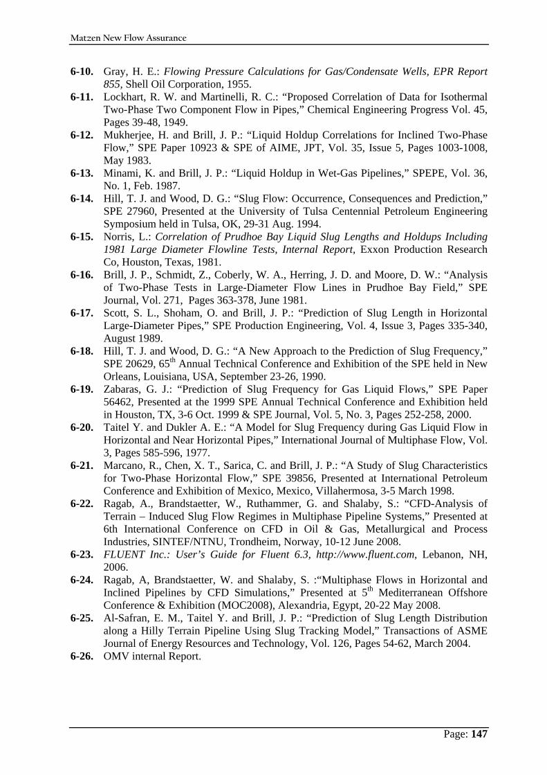
Matzen New Flow Assurance

Page: 147

6-10. Gray, H. E.: Flowing Pressure Calculations for Gas/Condensate Wells, EPR Report 855, Shell Oil Corporation, 1955.

6-11. Lockhart, R. W. and Martinelli, R. C.: “Proposed Correlation of Data for Isothermal Two-Phase Two Component Flow in Pipes,” Chemical Engineering Progress Vol. 45, Pages 39-48, 1949.

6-12. Mukherjee, H. and Brill, J. P.: “Liquid Holdup Correlations for Inclined Two-Phase Flow,” SPE Paper 10923 & SPE of AIME, JPT, Vol. 35, Issue 5, Pages 1003-1008, May 1983.

6-13. Minami, K. and Brill, J. P.: “Liquid Holdup in Wet-Gas Pipelines,” SPEPE, Vol. 36, No. 1, Feb. 1987.

6-14. Hill, T. J. and Wood, D. G.: “Slug Flow: Occurrence, Consequences and Prediction,” SPE 27960, Presented at the University of Tulsa Centennial Petroleum Engineering Symposium held in Tulsa, OK, 29-31 Aug. 1994.

6-15. Norris, L.: Correlation of Prudhoe Bay Liquid Slug Lengths and Holdups Including 1981 Large Diameter Flowline Tests, Internal Report, Exxon Production Research Co, Houston, Texas, 1981.

6-16. Brill, J. P., Schmidt, Z., Coberly, W. A., Herring, J. D. and Moore, D. W.: “Analysis of Two-Phase Tests in Large-Diameter Flow Lines in Prudhoe Bay Field,” SPE Journal, Vol. 271, Pages 363-378, June 1981.

6-17. Scott, S. L., Shoham, O. and Brill, J. P.: “Prediction of Slug Length in Horizontal Large-Diameter Pipes,” SPE Production Engineering, Vol. 4, Issue 3, Pages 335-340, August 1989.

6-18. Hill, T. J. and Wood, D. G.: “A New Approach to the Prediction of Slug Frequency,” SPE 20629, 65th Annual Technical Conference and Exhibition of the SPE held in New Orleans, Louisiana, USA, September 23-26, 1990.

6-19. Zabaras, G. J.: “Prediction of Slug Frequency for Gas Liquid Flows,” SPE Paper 56462, Presented at the 1999 SPE Annual Technical Conference and Exhibition held in Houston, TX, 3-6 Oct. 1999 & SPE Journal, Vol. 5, No. 3, Pages 252-258, 2000.

6-20. Taitel Y. and Dukler A. E.: “A Model for Slug Frequency during Gas Liquid Flow in Horizontal and Near Horizontal Pipes,” International Journal of Multiphase Flow, Vol. 3, Pages 585-596, 1977.

6-21. Marcano, R., Chen, X. T., Sarica, C. and Brill, J. P.: “A Study of Slug Characteristics for Two-Phase Horizontal Flow,” SPE 39856, Presented at International Petroleum Conference and Exhibition of Mexico, Mexico, Villahermosa, 3-5 March 1998.

6-22. Ragab, A., Brandstaetter, W., Ruthammer, G. and Shalaby, S.: “CFD-Analysis of Terrain – Induced Slug Flow Regimes in Multiphase Pipeline Systems,” Presented at 6th International Conference on CFD in Oil & Gas, Metallurgical and Process Industries, SINTEF/NTNU, Trondheim, Norway, 10-12 June 2008.

6-23. FLUENT Inc.: User’s Guide for Fluent 6.3, http://www.fluent.com, Lebanon, NH, 2006.

6-24. Ragab, A, Brandstaetter, W. and Shalaby, S. :“Multiphase Flows in Horizontal and Inclined Pipelines by CFD Simulations,” Presented at 5th Mediterranean Offshore Conference & Exhibition (MOC2008), Alexandria, Egypt, 20-22 May 2008.

6-25. Al-Safran, E. M., Taitel Y. and Brill, J. P.: “Prediction of Slug Length Distribution along a Hilly Terrain Pipeline Using Slug Tracking Model,” Transactions of ASME Journal of Energy Resources and Technology, Vol. 126, Pages 54-62, March 2004.

6-26. OMV internal Report.

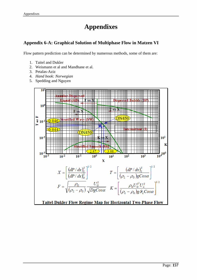
Appendixes

Page: 157

Appendixes

Appendix 6-A: Graphical Solution of Multiphase Flow in Matzen VI Flow pattern prediction can be determined by numerous methods, some of them are:

1. Taitel and Dukler 2. Weismann et al and Mandhane et al. 3. Petalas-Aziz 4. Hand book: Norwegian 5. Spedding and Nguyen

Appendixes

Page: 158

Appendixes

Page: 159

Appendix 6-B: Details of Liquid Holdup Calculations

I. Lockhart and Martinelli It was the first quantitative method proposed. It became classical for comparison with other later works. Basically, this approach is based on two main assumptions, firstly, the pressure drop for both gas and liquid are the same and secondly the total pipe volume equals the sum of the gas and liquid volumes. One aspect of the Lockhart-Martinelli correlation is that it skirts the flow pattern issue and applies for small diameter pipelines. Based on this previous statement, we tried to modify in order to calculate parameter-X of Lockhart-Martinelli Correlation using the modified equations for large pipe lines to be applicable for field pipeline diameters. In

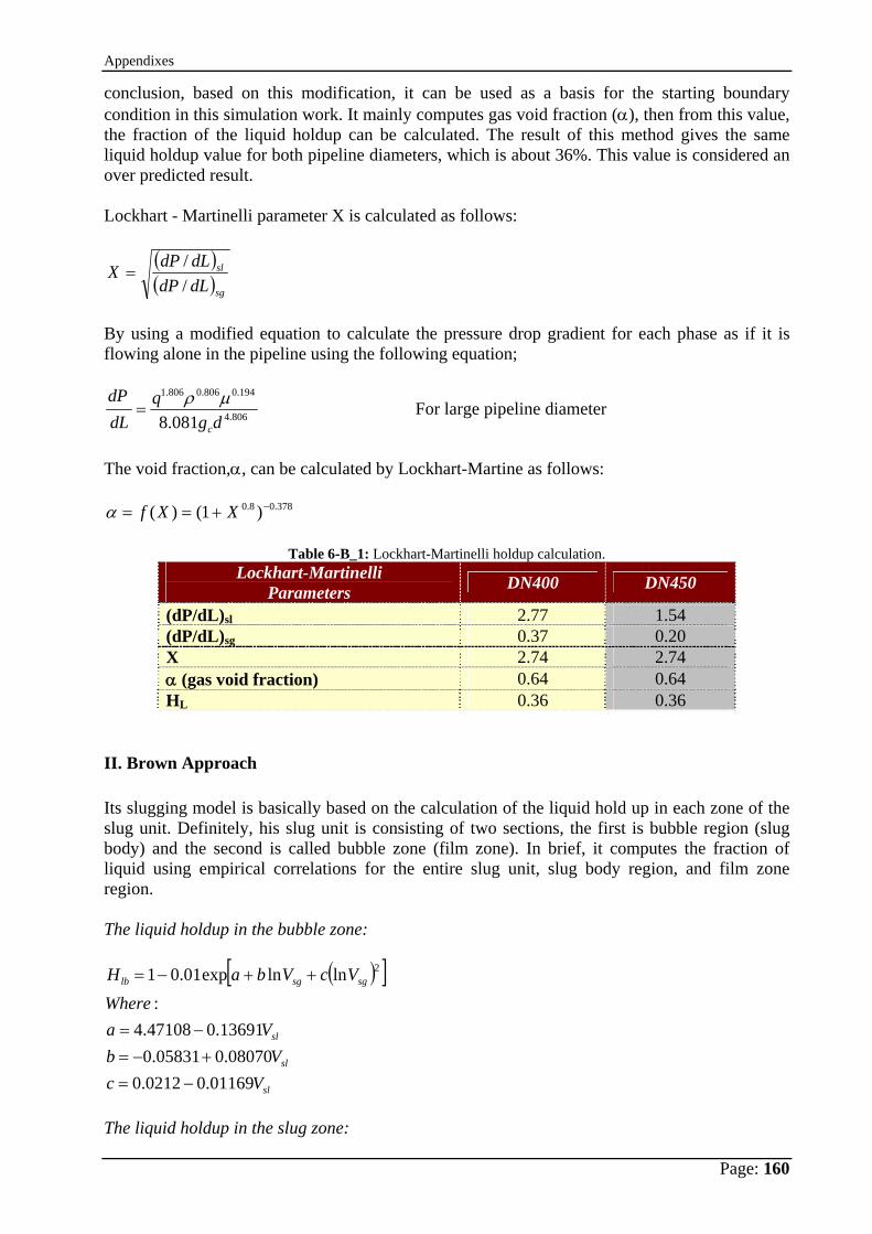
Appendixes

Page: 160

conclusion, based on this modification, it can be used as a basis for the starting boundary condition in this simulation work. It mainly computes gas void fraction (α), then from this value, the fraction of the liquid holdup can be calculated. The result of this method gives the same liquid holdup value for both pipeline diameters, which is about 36%. This value is considered an over predicted result. Lockhart - Martinelli parameter X is calculated as follows:

( )( )sg

sl

dLdPdLdPX

//

=

By using a modified equation to calculate the pressure drop gradient for each phase as if it is flowing alone in the pipeline using the following equation;

806.4

194.0806.0806.1

081.8 dgq

dLdP

c

μρ= For large pipeline diameter

The void fraction,α, can be calculated by Lockhart-Martine as follows:

378.08.0 )1()( −+== XXfα

Table 6-B_1: Lockhart-Martinelli holdup calculation. Lockhart-Martinelli

Parameters DN400 DN450

(dP/dL)sl 2.77 1.54 (dP/dL)sg 0.37 0.20 X 2.74 2.74 α (gas void fraction) 0.64 0.64 HL 0.36 0.36

II. Brown Approach Its slugging model is basically based on the calculation of the liquid hold up in each zone of the slug unit. Definitely, his slug unit is consisting of two sections, the first is bubble region (slug body) and the second is called bubble zone (film zone). In brief, it computes the fraction of liquid using empirical correlations for the entire slug unit, slug body region, and film zone region. The liquid holdup in the bubble zone:

( )[ ]

sl

sl

sl

sgsglb

VcVb

VaWhere

VcVbaH

01169.00212.008070.005831.0

13691.047108.4:

lnlnexp01.01 2

−=+−=

−=

++−=

The liquid holdup in the slug zone:

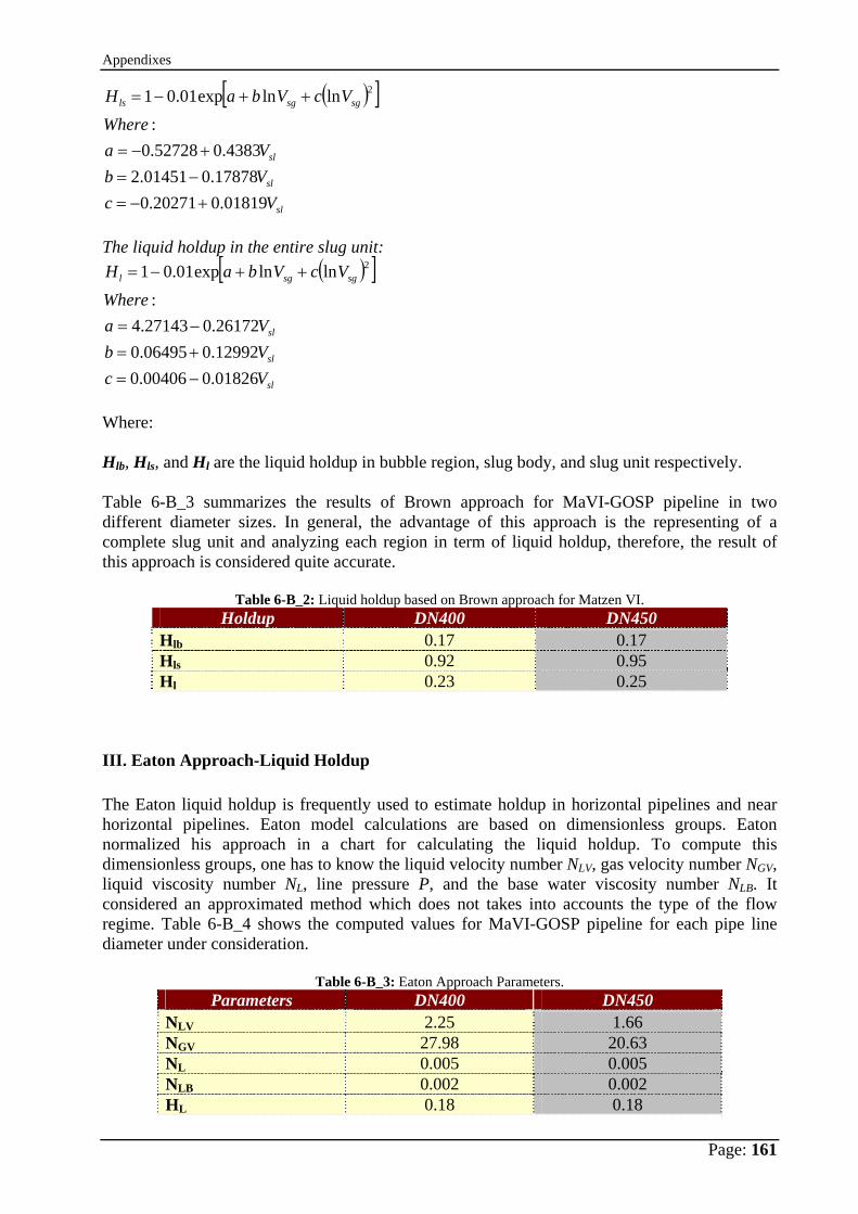
Appendixes

Page: 161

( )[ ]

sl

sl

sl

sgsgls

VcVbVa

WhereVcVbaH

01819.020271.017878.001451.2

4383.052728.0:

lnlnexp01.01 2

+−=−=

+−=

++−=

The liquid holdup in the entire slug unit:

( )[ ]

sl

sl

sl

sgsgl

VcVbVa

WhereVcVbaH

01826.000406.012992.006495.026172.027143.4

:lnlnexp01.01 2

−=+=−=

++−=

Where: Hlb, Hls, and Hl are the liquid holdup in bubble region, slug body, and slug unit respectively. Table 6-B_3 summarizes the results of Brown approach for MaVI-GOSP pipeline in two different diameter sizes. In general, the advantage of this approach is the representing of a complete slug unit and analyzing each region in term of liquid holdup, therefore, the result of this approach is considered quite accurate.

Table 6-B_2: Liquid holdup based on Brown approach for Matzen VI. Holdup DN400 DN450

Hlb 0.17 0.17 Hls 0.92 0.95 Hl 0.23 0.25

III. Eaton Approach-Liquid Holdup The Eaton liquid holdup is frequently used to estimate holdup in horizontal pipelines and near horizontal pipelines. Eaton model calculations are based on dimensionless groups. Eaton normalized his approach in a chart for calculating the liquid holdup. To compute this dimensionless groups, one has to know the liquid velocity number NLV, gas velocity number NGV, liquid viscosity number NL, line pressure P, and the base water viscosity number NLB. It considered an approximated method which does not takes into accounts the type of the flow regime. Table 6-B_4 shows the computed values for MaVI-GOSP pipeline for each pipe line diameter under consideration.

Table 6-B_3: Eaton Approach Parameters. Parameters DN400 DN450

NLV 2.25 1.66 NGV 27.98 20.63 NL 0.005 0.005 NLB 0.002 0.002 HL 0.18 0.18

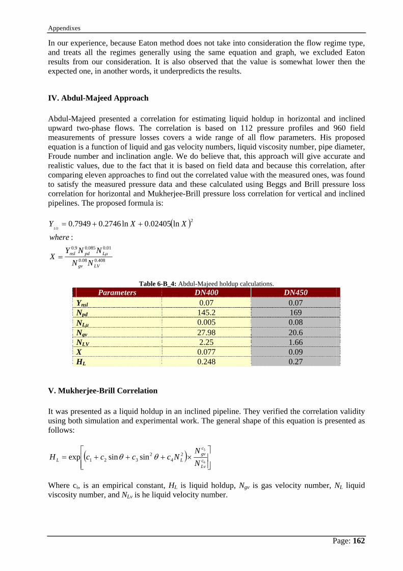
Appendixes

Page: 162

In our experience, because Eaton method does not take into consideration the flow regime type, and treats all the regimes generally using the same equation and graph, we excluded Eaton results from our consideration. It is also observed that the value is somewhat lower then the expected one, in another words, it underpredicts the results.

IV. Abdul-Majeed Approach Abdul-Majeed presented a correlation for estimating liquid holdup in horizontal and inclined upward two-phase flows. The correlation is based on 112 pressure profiles and 960 field measurements of pressure losses covers a wide range of all flow parameters. His proposed equation is a function of liquid and gas velocity numbers, liquid viscosity number, pipe diameter, Froude number and inclination angle. We do believe that, this approach will give accurate and realistic values, due to the fact that it is based on field data and because this correlation, after comparing eleven approaches to find out the correlated value with the measured ones, was found to satisfy the measured pressure data and these calculated using Beggs and Brill pressure loss correlation for horizontal and Mukherjee-Brill pressure loss correlation for vertical and inclined pipelines. The proposed formula is:

( )

408.008.0

01.0085.09.0

2

:

ln02405.0ln2746.07949.0

LVgv

Lpdnsl

NNNNY

X

where

XXYLO

μ=

++=

Table 6-B_4: Abdul-Majeed holdup calculations.

Parameters DN400 DN450 Ynsl 0.07 0.07 Npd 145.2 169 NLμ 0.005 0.08 Ngv 27.98 20.6 NLV 2.25 1.66 X 0.077 0.09 HL 0.248 0.27

V. Mukherjee-Brill Correlation It was presented as a liquid holdup in an inclined pipeline. They verified the correlation validity using both simulation and experimental work. The general shape of this equation is presented as follows:

( )⎥⎥⎦

⎤

⎢⎢⎣

⎡×+++=

6

52

42

321 sinsinexp cLv

cgv

LL NN

NccccH θθ

Where ci, is an empirical constant, HL is liquid holdup, Ngv is gas velocity number, NL liquid viscosity number, and NLv is he liquid velocity number.

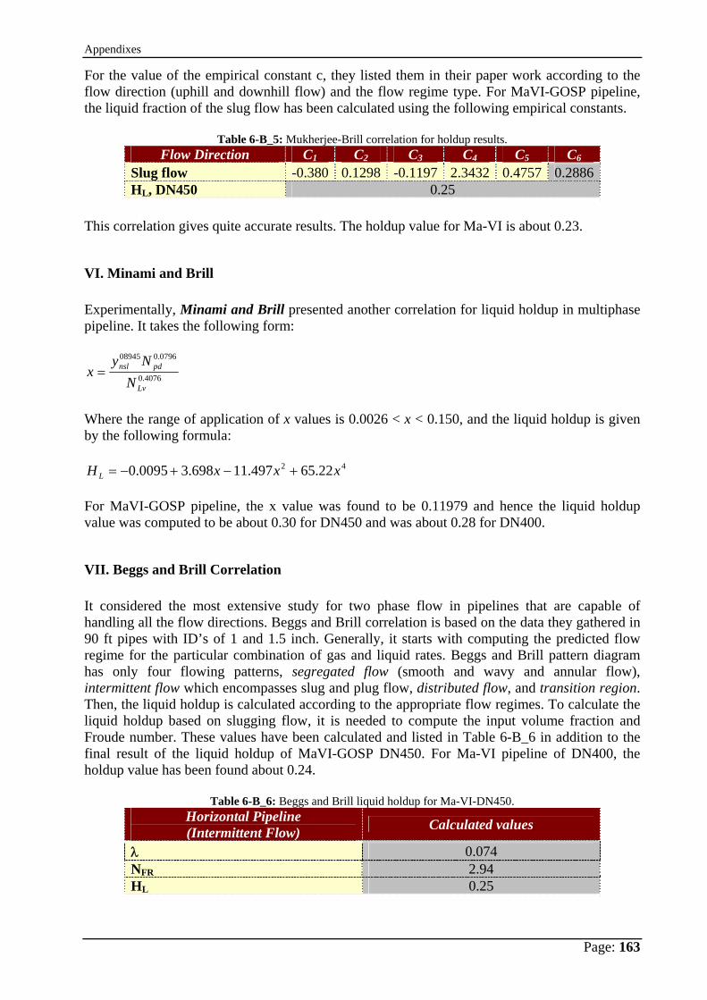
Appendixes

Page: 163

For the value of the empirical constant c, they listed them in their paper work according to the flow direction (uphill and downhill flow) and the flow regime type. For MaVI-GOSP pipeline, the liquid fraction of the slug flow has been calculated using the following empirical constants.

Table 6-B_5: Mukherjee-Brill correlation for holdup results. Flow Direction C1 C2 C3 C4 C5 C6

Slug flow -0.380 0.1298 -0.1197 2.3432 0.4757 0.2886HL, DN450 0.25

This correlation gives quite accurate results. The holdup value for Ma-VI is about 0.23.

VI. Minami and Brill Experimentally, Minami and Brill presented another correlation for liquid holdup in multiphase pipeline. It takes the following form:

4076.0

0796.008945

Lv

pdnsl

NNy

x =

Where the range of application of x values is 0.0026 < x < 0.150, and the liquid holdup is given by the following formula:

42 22.65497.11698.30095.0 xxxH L +−+−= For MaVI-GOSP pipeline, the x value was found to be 0.11979 and hence the liquid holdup value was computed to be about 0.30 for DN450 and was about 0.28 for DN400.

VII. Beggs and Brill Correlation It considered the most extensive study for two phase flow in pipelines that are capable of handling all the flow directions. Beggs and Brill correlation is based on the data they gathered in 90 ft pipes with ID’s of 1 and 1.5 inch. Generally, it starts with computing the predicted flow regime for the particular combination of gas and liquid rates. Beggs and Brill pattern diagram has only four flowing patterns, segregated flow (smooth and wavy and annular flow), intermittent flow which encompasses slug and plug flow, distributed flow, and transition region. Then, the liquid holdup is calculated according to the appropriate flow regimes. To calculate the liquid holdup based on slugging flow, it is needed to compute the input volume fraction and Froude number. These values have been calculated and listed in Table 6-B_6 in addition to the final result of the liquid holdup of MaVI-GOSP DN450. For Ma-VI pipeline of DN400, the holdup value has been found about 0.24.

Table 6-B_6: Beggs and Brill liquid holdup for Ma-VI-DN450. Horizontal Pipeline (Intermittent Flow) Calculated values

λ 0.074 NFR 2.94 HL 0.25

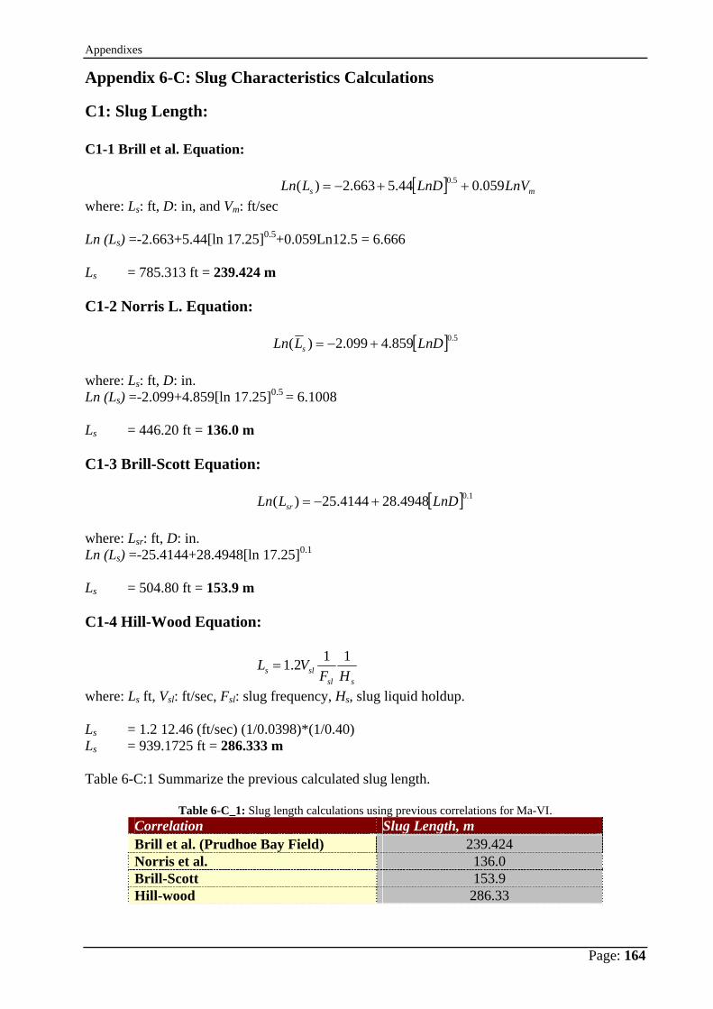
Appendixes

Page: 164

Appendix 6-C: Slug Characteristics Calculations

C1: Slug Length: C1-1 Brill et al. Equation:

[ ] ms LnVLnDLLn 059.044.5663.2)( 5.0 ++−= where: Ls: ft, D: in, and Vm: ft/sec Ln (Ls) =-2.663+5.44[ln 17.25]0.5+0.059Ln12.5 = 6.666 Ls = 785.313 ft = 239.424 m C1-2 Norris L. Equation:

[ ] 5.0859.4099.2)( LnDLLn s +−=

where: Ls: ft, D: in. Ln (Ls) =-2.099+4.859[ln 17.25]0.5 = 6.1008 Ls = 446.20 ft = 136.0 m C1-3 Brill-Scott Equation:

[ ] 1.04948.284144.25)( LnDLLn sr +−= where: Lsr: ft, D: in. Ln (Ls) =-25.4144+28.4948[ln 17.25]0.1

Ls = 504.80 ft = 153.9 m C1-4 Hill-Wood Equation:

sslsls HF

VL 112.1=

where: Ls ft, Vsl: ft/sec, Fsl: slug frequency, Hs, slug liquid holdup. Ls = 1.2 12.46 (ft/sec) (1/0.0398)*(1/0.40) Ls = 939.1725 ft = 286.333 m Table 6-C:1 Summarize the previous calculated slug length.

Table 6-C_1: Slug length calculations using previous correlations for Ma-VI.

Correlation Slug Length, m Brill et al. (Prudhoe Bay Field) 239.424 Norris et al. 136.0 Brill-Scott 153.9 Hill-wood 286.33

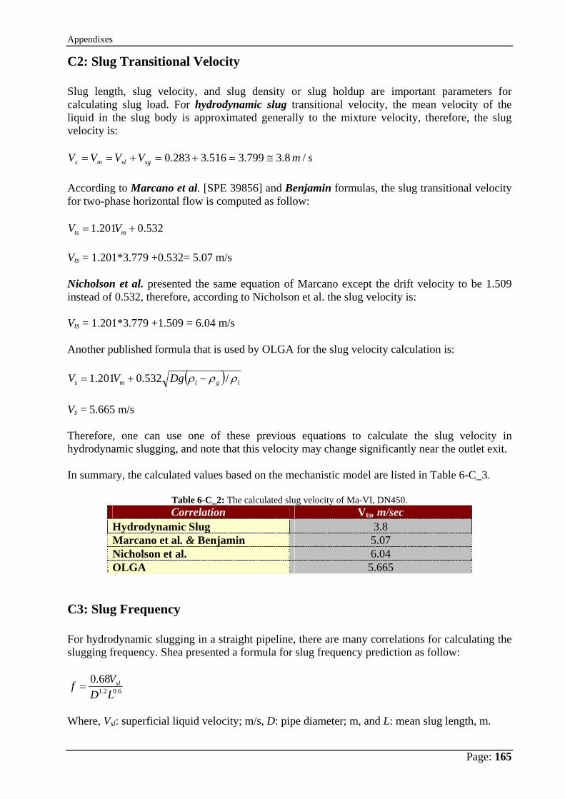
Appendixes

Page: 165

C2: Slug Transitional Velocity Slug length, slug velocity, and slug density or slug holdup are important parameters for calculating slug load. For hydrodynamic slug transitional velocity, the mean velocity of the liquid in the slug body is approximated generally to the mixture velocity, therefore, the slug velocity is:

smVVVV sgslms / 8.3799.3516.3283.0 ≅=+=+== According to Marcano et al. [SPE 39856] and Benjamin formulas, the slug transitional velocity for two-phase horizontal flow is computed as follow:

532.0201.1 += mts VV Vts = 1.201*3.779 +0.532= 5.07 m/s Nicholson et al. presented the same equation of Marcano except the drift velocity to be 1.509 instead of 0.532, therefore, according to Nicholson et al. the slug velocity is: Vts = 1.201*3.779 +1.509 = 6.04 m/s Another published formula that is used by OLGA for the slug velocity calculation is:

( ) lglms DgVV ρρρ /532.0201.1 −+= Vs = 5.665 m/s Therefore, one can use one of these previous equations to calculate the slug velocity in hydrodynamic slugging, and note that this velocity may change significantly near the outlet exit. In summary, the calculated values based on the mechanistic model are listed in Table 6-C_3.

Table 6-C_2: The calculated slug velocity of Ma-VI, DN450. Correlation Vts, m/sec

Hydrodynamic Slug 3.8 Marcano et al. & Benjamin 5.07 Nicholson et al. 6.04 OLGA 5.665

C3: Slug Frequency For hydrodynamic slugging in a straight pipeline, there are many correlations for calculating the slugging frequency. Shea presented a formula for slug frequency prediction as follow:

6.02.168.0

LDVf sl=

Where, Vsl: superficial liquid velocity; m/s, D: pipe diameter; m, and L: mean slug length, m.

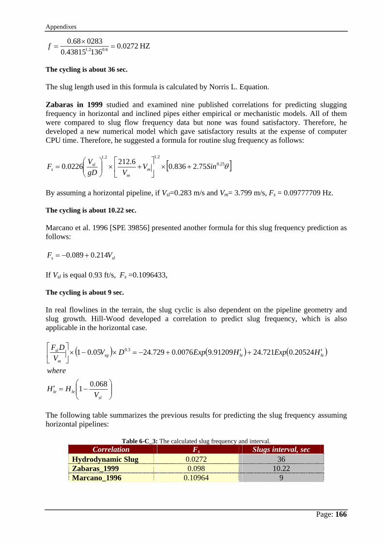
Appendixes

Page: 166

HZ0272.013643815.0

028368.06.02.1 =

×=f

The cycling is about 36 sec. The slug length used in this formula is calculated by Norris L. Equation. Zabaras in 1999 studied and examined nine published correlations for predicting slugging frequency in horizontal and inclined pipes either empirical or mechanistic models. All of them were compared to slug flow frequency data but none was found satisfactory. Therefore, he developed a new numerical model which gave satisfactory results at the expense of computer CPU time. Therefore, he suggested a formula for routine slug frequency as follows:

[ ]θ25.02.12.1

75.2836.06.2120226.0 SinVVgD

VF mm

sls +×⎥

⎦

⎤⎢⎣

⎡+×⎟⎟

⎠

⎞⎜⎜⎝

⎛=

By assuming a horizontal pipeline, if Vsl=0.283 m/s and Vm= 3.799 m/s, Fs = 0.09777709 Hz. The cycling is about 10.22 sec. Marcano et al. 1996 [SPE 39856] presented another formula for this slug frequency prediction as follows:

sls VF 214.0089.0 +−= If Vsl is equal 0.93 ft/s, Fs =0.1096433, The cycling is about 9 sec. In real flowlines in the terrain, the slug cyclic is also dependent on the pipeline geometry and slug growth. Hill-Wood developed a correlation to predict slug frequency, which is also applicable in the horizontal case.

( ) ( ) ( )

⎟⎟⎠

⎞⎜⎜⎝

⎛−=′

′+′+−=×−×⎥⎦

⎤⎢⎣

⎡

sllele

lelesgm

sl

VHH

where

HExpHExpDVV

DF

068.01

20524.0721.2491209.90076.0729.2405.01 3.0

The following table summarizes the previous results for predicting the slug frequency assuming horizontal pipelines:

Table 6-C_3: The calculated slug frequency and interval. Correlation Fs Slugs interval, sec

Hydrodynamic Slug 0.0272 36 Zabaras_1999 0.098 10.22 Marcano_1996 0.10964 9

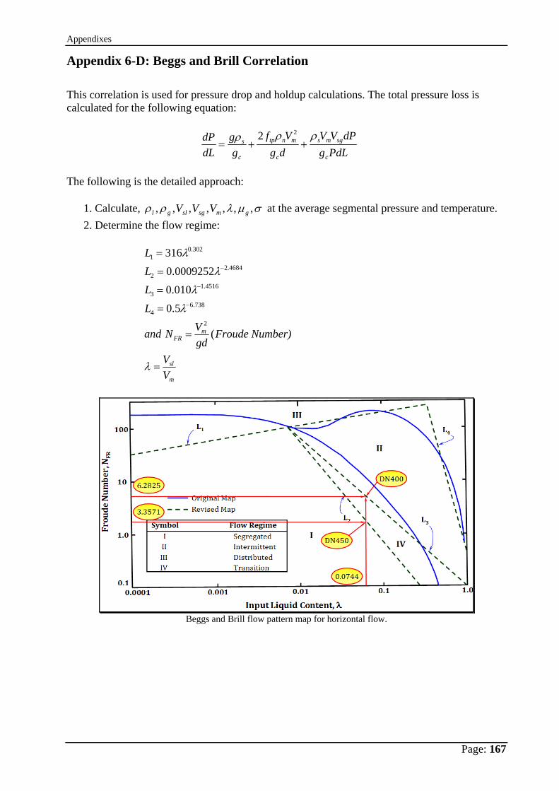
Appendixes

Page: 167

Appendix 6-D: Beggs and Brill Correlation This correlation is used for pressure drop and holdup calculations. The total pressure loss is calculated for the following equation:

PdLgdPVV

dgVf

gg

dLdP

c

sgms

c

mntp

c

s ρρρ++=

22

The following is the detailed approach:

1. Calculate, σμλρρ ,,,,,,, gmsgslgl VVV at the average segmental pressure and temperature. 2. Determine the flow regime:

m

sl

mFR

VV

Number) FroudegdVN and

L

LLL

=

=

=

=

=

=

−

−

−

λ

λ

λ

λ

λ

(

5.0

010.00009252.0

316

2

738.64

4516.13

4684.22

302.01

Beggs and Brill flow pattern map for horizontal flow.

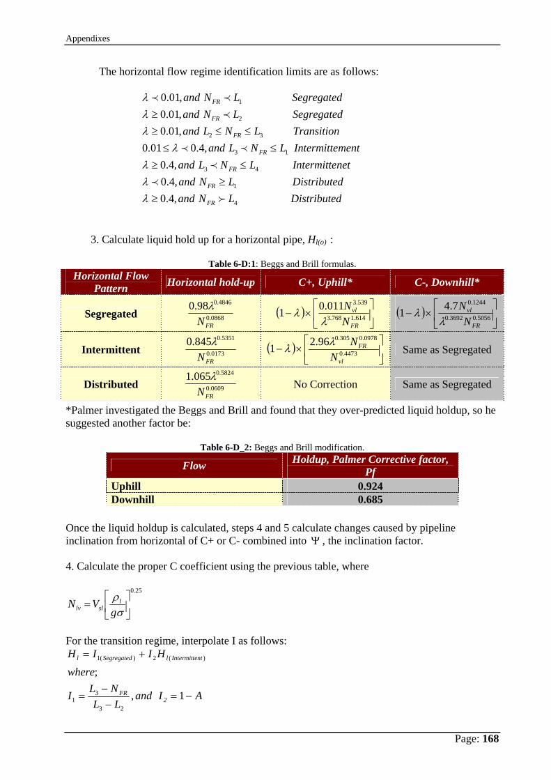
Appendixes

Page: 168

The horizontal flow regime identification limits are as follows:

dDistribute LN anddDistribute LN andnetIntermitte LNL andmentIntermitte LNL and

Transition LNL andgregated Se LN andgregated Se LN and

FR

FR

FR

FR

FR

FR

FR

4

1

43

13

32

2

1

,4.0,4.0,4.0

,4.001.0,01.0,01.0,01.0

f

p

p

pp

p

pp

≥≥

≤≥≤≤

≤≤≥≥

λλλ

λλλλ

3. Calculate liquid hold up for a horizontal pipe, Hl(o) :

Table 6-D:1: Beggs and Brill formulas. Horizontal Flow

Pattern Horizontal hold-up C+, Uphill* C-, Downhill*

Segregated 0868.0

4846.098.0

FRNλ ( ) ⎥

⎦

⎤⎢⎣

⎡×− 614.1768.3

539.3011.01FR

vl

NN

λλ ( ) ⎥

⎦

⎤⎢⎣

⎡×− 5056.03692.0

1244.07.41FR

vl

NN

λλ

Intermittent 0173.0

5351.0845.0

FRNλ ( ) ⎥

⎦

⎤⎢⎣

⎡×− 4473.0

0978.0305.096.21vl

FR

NNλλ Same as Segregated

Distributed 0609.0

5824.0065.1

FRNλ No Correction Same as Segregated

*Palmer investigated the Beggs and Brill and found that they over-predicted liquid holdup, so he suggested another factor be:

Table 6-D_2: Beggs and Brill modification.

Flow Holdup, Palmer Corrective factor, Pf

Uphill 0.924 Downhill 0.685

Once the liquid holdup is calculated, steps 4 and 5 calculate changes caused by pipeline inclination from horizontal of C+ or C- combined into Ψ , the inclination factor. 4. Calculate the proper C coefficient using the previous table, where

25.0

⎥⎦

⎤⎢⎣

⎡=

σρg

VN lsllv

For the transition regime, interpolate I as follows:

AI andLL

NLI

whereHIIH

2FR

ntIntermittelSegregatedl

−=−

−=

+=

1,

;

23

31

)(2)(1

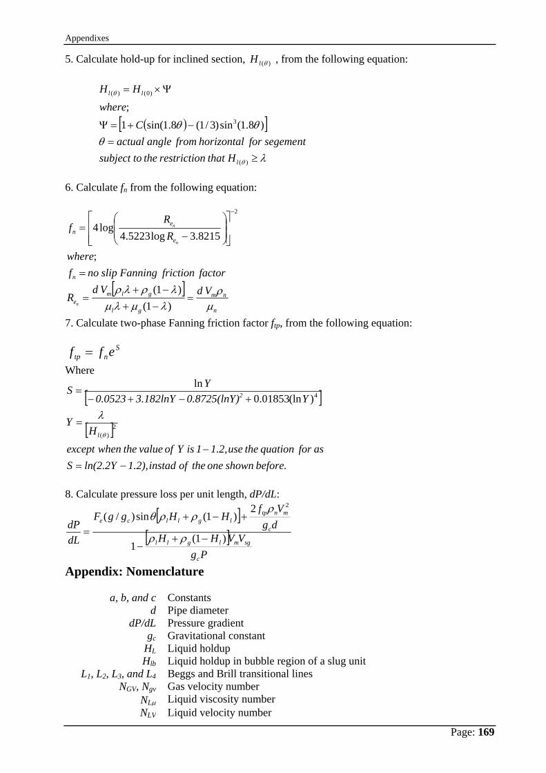
Appendixes

Page: 169

5. Calculate hold-up for inclined section, )(θlH , from the following equation:

( )[ ]

λθ

θθ

θ

θ

≥=

−+=Ψ

Ψ×=

)(

3

)0()(

)8.1(sin)3/1(8.1sin(1;

l

ll

H that nrestrictio the to subject ntfor segeme horizontal from angle actual

Cwhere

HH

6. Calculate fn from the following equation:

[ ]n

nm

gl

glme

n

e

en

V dV dR

factor friction Fanning slipno fwhere

RR

f

n

n

n

μρ

λμλμλρλρ

=−+

−+=

=

⎥⎥⎦

⎤

⎢⎢⎣

⎡⎟⎟⎠

⎞⎜⎜⎝

⎛

−=

−

)1()1(

;

8215.3log5223.4log4

2

7. Calculate two-phase Fanning friction factor ftp, from the following equation:

Sntp eff =

Where

[ ]

[ ]

before. shownone the of instad 1.2),ln(2.2YS

asfor quation the use 1.2,1 is Y of value the whenexceptH

Y

Y)0.8725(lnY3.182lnY0.0523Y S

l

2

−=−

=

+−+−=

2)(

4)(ln01853.0ln

θ

λ

8. Calculate pressure loss per unit length, dP/dL:

[ ][ ]

PgVVHH

dgVf

HHggF

dLdP

c

sgmlgll

c

mntplgllce

)1(1

2)1(sin)/(

2

−+−

+−+= ρρ

ρρρθ

Appendix: Nomenclature

a, b, and c Constants d Pipe diameter

dP/dL Pressure gradient gc Gravitational constant

HL Liquid holdup Hlb Liquid holdup in bubble region of a slug unit

L1, L2, L3, and L4 Beggs and Brill transitional lines NGV, Ngv Gas velocity number

NLμ Liquid viscosity number NLV Liquid velocity number

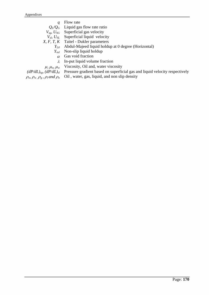
Appendixes

Page: 170

q Flow rate QL/QG Liquid gas flow rate ratio

Vsg, USG Superficial gas velocity Vsl, USL Superficial liquid velocity

X, F, T, K Taitel - Dukler parameters YL0 Abdul-Majeed liquid holdup at 0 degree (Horizontal) Ynsl Non-slip liquid holdup

α Gas void fraction λ In-put liquid volume fraction

μ, μo, μw Viscosity, Oil and, water viscosity (dP/dL)sg, (dP/dL)sl Pressure gradient based on superficial gas and liquid velocity respectivelyρo, ρw , ρg , ρl and ρn Oil , water, gas, liquid, and non slip density

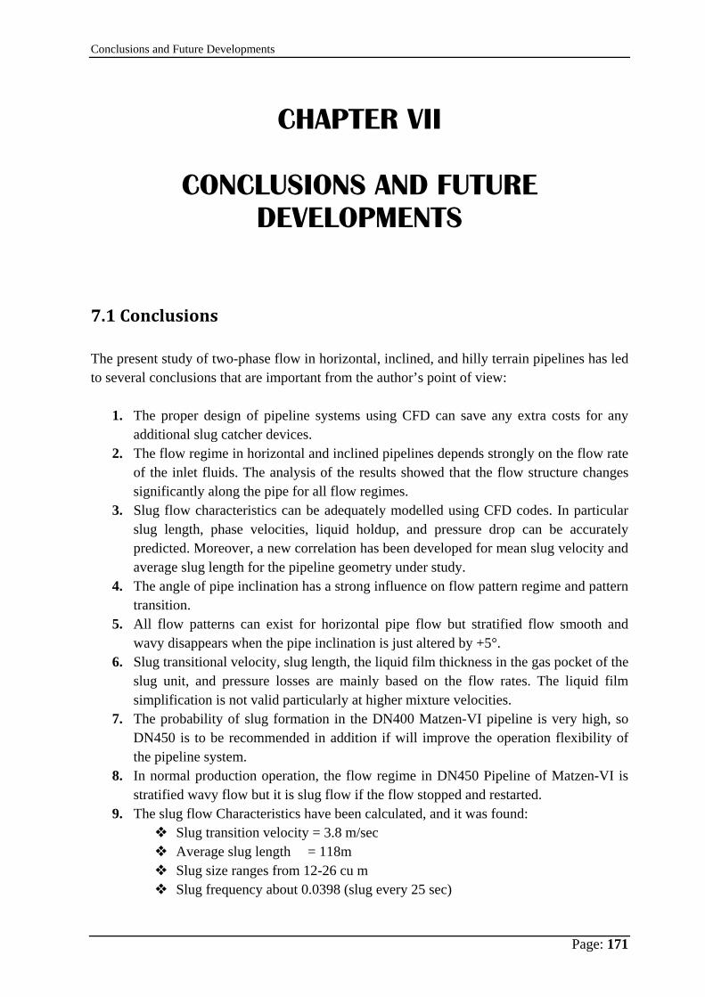
Conclusions and Future Developments

Page: 171

CHAPTER VII

CONCLUSIONS AND FUTURE

DEVELOPMENTS

7.1 Conclusions  The present study of two-phase flow in horizontal, inclined, and hilly terrain pipelines has led to several conclusions that are important from the author’s point of view:

1. The proper design of pipeline systems using CFD can save any extra costs for any additional slug catcher devices.

2. The flow regime in horizontal and inclined pipelines depends strongly on the flow rate of the inlet fluids. The analysis of the results showed that the flow structure changes significantly along the pipe for all flow regimes.

3. Slug flow characteristics can be adequately modelled using CFD codes. In particular slug length, phase velocities, liquid holdup, and pressure drop can be accurately predicted. Moreover, a new correlation has been developed for mean slug velocity and average slug length for the pipeline geometry under study.

4. The angle of pipe inclination has a strong influence on flow pattern regime and pattern transition.

5. All flow patterns can exist for horizontal pipe flow but stratified flow smooth and wavy disappears when the pipe inclination is just altered by +5°.

6. Slug transitional velocity, slug length, the liquid film thickness in the gas pocket of the slug unit, and pressure losses are mainly based on the flow rates. The liquid film simplification is not valid particularly at higher mixture velocities.

7. The probability of slug formation in the DN400 Matzen-VI pipeline is very high, so DN450 is to be recommended in addition if will improve the operation flexibility of the pipeline system.

8. In normal production operation, the flow regime in DN450 Pipeline of Matzen-VI is stratified wavy flow but it is slug flow if the flow stopped and restarted.

9. The slug flow Characteristics have been calculated, and it was found: Slug transition velocity = 3.8 m/sec Average slug length = 118m Slug size ranges from 12-26 cu m Slug frequency about 0.0398 (slug every 25 sec)

Conclusions and Future Developments

Page: 172

10. These results are in a good agreement with an earlier study performed by Petrofac

company in terms of slug volume and pressure drop calculations. 11. The calculated pressure drop for the whole Matzen-VI pipeline of DN450 is 0.62 bars

by using CFD calculation.

7.2 Future Developments and Recommendations  During the last three years from this research work, a lot of new questions appeared. Some of them have already been answered in this thesis, and in the seven published papers in journal and conferences, but there is a still a list of further research developments and possibilities. The following list gives a hint of them being closely related to the present dissertation:

1. More numerical investigations should be made to study the slug body itself, to determine the gas void fraction in each slug and how it affects the length of each slug.

2. Application of this new technique to model the multiphase fluid flow in a vertical

pipeline to see how these fluids react while oil production in the vertical well.

3. More concentrations on modeling the transition zones between each two flow regimes, specially between stratified and slug flow regimes in long hilly terrain pipelines.

4. A comparison should be made between the CFD simulation results and a field scale

pipeline data