Observational constraints on the types of cosmic strings

Eur. Phys. J. C (2014) 74:2972DOI 10.1140/epjc/s10052-014-2972-6

Regular Article - Theoretical Physics

Observational constraints on the types of cosmic strings

Olga S. Sazhina1,a, Diana Scognamiglio2,b, Mikhail V. Sazhin1,c

1 Moscow M.V. Lomonosov State University, Sternberg Astronomical Institute (SAI MSU), 13, Universitetskij pr., Moscow 119992, Russia2 University of Naples Federico II, via Cinthia, 6, 80126 Naples, Italy

Received: 30 June 2014 / Accepted: 8 July 2014© The Author(s) 2014. This article is published with open access at Springerlink.com

Abstract This paper is aimed at setting observational lim-its to the number of cosmic strings (Nambu–Goto, Abelian-Higgs, semilocal) and other topological defects (textures).Radio maps of CMB anisotropy, provided by the space mis-sion Planck for various frequencies, were filtered and thenprocessed by the method of convolution with modified Haarfunctions (MHF) to search for cosmic string candidates. Thismethod was designed to search for solitary strings, with-out additional assumptions as regards the presence of net-works of such objects. The sensitivity of the MHF method isδT ≈ 10 µK in a background of δT ≈ 100 µK. The com-parison of these with previously known results on searchstring network shows that strings can only be semilocal inthe range of 1 ÷ 5, with the upper restriction on individualstring tension (linear density) of Gμ/c2 ≤ 7.36 × 10−7.The texture model is also legal. There are no strings withGμ/c2 > 7.36×10−7. However, a comparison with the datafor the search of non-Gaussian signals shows that the pres-ence of several (up to three) Nambu–Goto strings is also pos-sible. For Gμ/c2 ≤ 4.83×10−7 the MHF method is ineffec-tive because of unverifiable spurious string candidates. Thusthe existence of strings with tensions Gμ/c2 ≤ 4.83 × 10−7

is not prohibited but it is beyond the Planck data possibilities.The same string candidates have been found in the WMAP9-year data. Independence of Planck and WMAP data setsserves as an additional argument to consider those string can-didates as very promising. However, the final proof shouldbe given by optical deep surveys.

1 Introduction

The expansion and cooling of the Universe took place in sev-eral phases of transition, while different types of topological

a e-mail: [email protected] e-mail: [email protected] e-mail: [email protected]

defects were formed. The best known topological defects arecosmic strings (CS), whose topological structure of the sym-metry breaking at the phase transition ensures their stability.CS were postulated by Kibble [1] and immediately became ahot issue in both theoretical physics and cosmology [2,3]. Itcan be stated that topological CS are infinitely long and fil-amentary remnants of primordial dark energy (high energysymmetric vacuum) which formed in the early Universe andwere then stretched by the cosmological expansion up tothe point that, at the present epoch, some CS could cross theentire length of the observable Universe. The detection of CSwould allow us to disentangle the true underlying theoreti-cal framework and to extend our experimental knowledge inthe GUT energy domain which is unavailable to modern andforeseen particle accelerators (i.e. 1014÷1016 GeV). It wouldalso allow us to confirm on observational grounds some ofthe key points of inflation theory. CS formation appears to beubiquitous in GUT theories and in fundamental superstringtheory. Therefore, the models with non-topological defects,called semilocal strings, have become quite popular (see [4]and references therein).

Active search for observational manifestations of CS, aswell as probabilistic estimations of their number [5], showthat, whether or not they exist, CS should be very few.

2 Methods of CS observational search

A CS produces the peculiar conical topology of the space-time and it may cause a detectable effects both in radio andin optical data. Modern strategies for detecting CS can besubdivided in three main classes:

1. detection through gravitational lensing effects. Themethod is based on the extensive monitoring of deep opti-cal surveys [6–10]. The aim is to find chains of pairs ofvirtual and particularly truncated galaxy images which aCS is expected to produce;

123

2972 Page 2 of 10 Eur. Phys. J. C (2014) 74:2972

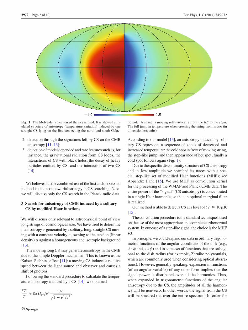
Fig. 1 The Molveide projection of the sky is used. It is showed sim-ulated structure of anisotropy (temperature variation) induced by onestraight CS lying on the line connecting the north and south Galac-

tic pole. A string is moving relativistically from the left to the right.The full jump in temperature when crossing the string front is two (indimensionless units)

2. detection through the signatures left by CS on the CMBanisotropy [11–13];

3. detection of model depended and rare features such as, forinstance, the gravitational radiation from CS loops, theinteractions of CS with black holes, the decay of heavyparticles emitted by CS, and the interaction of two CS[14].

We believe that the combined use of the first and the secondmethod is the most powerful strategy in CS searching. Next,we will discuss only the CS search in the Planck radio data.

3 Search for anisotropy of CMB induced by a solitaryCS by modified Haar functions

We will discuss only relevant to astrophysical point of viewlong strings of cosmological size. We have tried to determineif anisotropy is generated by a solitary, long, straight CS mov-ing with a constant velocity v, owning to the tension (lineardensity) μ against a homogeneous and isotropic background[13].

The moving long CS may generate anisotropy in the CMBdue to the simple Doppler mechanism. This is known as theKaiser–Stebbins effect [11]: a moving CS induces a relativespeed between the light source and observer and causes ashift of photons.

Following the standard procedure to calculate the temper-ature anisotropy induced by a CS [14], we obtained

δT

T≈ 8πGμ/c2 v/c

√1 − v2/c2

.

According to our model [13], an anisotropy induced by soli-tary CS represents a sequence of zones of decreased andincreased temperature: the cold spot in front of moving string,the step-like jump, and then appearance of hot spot; finally acold spot follows again (Fig. 1).

Due to the specific discontinuity structure of CS anisotropyand its low amplitude we searched its traces with a spe-cial step-like set of modified Haar functions (MHF); seeAppendix I and [15]. We use MHF as convolution kernelfor the processing of the WMAP and Planck CMB data. Theentire power of the “signal” (CS anisotropy) is concentratedin a single Haar harmonic, so that an optimal marginal filteris realized.

Our method is able to detect a CS at a level of δT ≈ 10 µK[15].

The convolution procedure is the standard technique basedon the use of the most appropriate and complete orthonormalsystem. In our case of a step-like signal the choice is the MHFset.

In principle, we could expand our data in ordinary trigono-metric functions of the angular coordinate of the disk (e.g.,sin φ and cosφ) and in some set of functions that are orthog-onal to the disk radius (for example, Zernike polynomials,which are commonly used when considering optical aberra-tions). However, generally speaking, expansion in functions(of an angular variable) of any other form implies that thesignal power is distributed over all the harmonics. Thus,when expanded in trigonometric functions of the angularanisotropy due to the CS, the amplitudes of all the harmon-ics will be non-zero. In other words, the signal from the CSwill be smeared out over the entire spectrum. In order for

123

Eur. Phys. J. C (2014) 74:2972 Page 3 of 10 2972

Fig. 2 Cleaned Planck data (143 GHz, units are [K]). 70 % Galaxy mask and point source extractors are used

the signal to be detected, the power smeared out over all theharmonics must be “gathered” to make use of the full powerof the signal.

For our purpose the MHF is a realization of the first har-monic of the Haar system of orthogonal functions with cyclicshift. This function is equal to 1 in the rotation range [0, π),and it is equal to −1 in the rotation range [π, 2π). Since aCS could be oriented arbitrarily with respect to a grid of linesof longitude and latitude, the search for a CS at each pointrequires multiple convolutions with a rotation of the circle,which corresponds to a shift in the “jump” in the Haar func-tion. This shift yields a new orthogonal and complete set offunctions: MHF. The rotations result in a set of amplitudes.When there is a CS at a convolution point, the harmonic ismaximum if a chord of the circle coincides with the positionof the CS. We assigned each pixel a value equal to the cor-responding maximum value of the convolution, in this waymaking a map of CS candidates (see Fig. 3).

Before the MHF algorithm was applied on real data weestimated its efficiency and chose the optimal convolutioncircle radius.

We applied MHF algorithm to process a map that wasa sum of two model maps. The first map was a simulatedmap of the primordial CMB anisotropy that arose at the sur-face of last scattering. We generated 300 such maps startingfrom a simulated power spectrum, generated by CMBEASY[16,17], a lighter and faster version of CMBFAST. The sec-ond map was a pure anisotropy generated by a straight, mov-ing CS (see Fig. 1 as an example of such map). The mapsof the primordial CMB anisotropy and the anisotropy gen-erated by the moving CS were summed with a coefficient to

characterize the signal-to-noise ratio. To choose an optimalcircle radius for a search for CS, we performed computer sim-ulations to obtain maps of the distribution of the harmonicamplitude for circles with various radii. We characterizedthe CS detection by the signal-to-noise ratio, since the CSposition in the model maps was known. The amplitude at theCS location was taken to be the signal and the rms of theharmonic amplitude in the map to be the noise. Those sim-ulations indicate that the optimal value of the convolutioncircle radius is from 3◦ to 5◦.

In order to study the efficiency of the MHF algorithm wealso apply statistical methods of simulations. We created arobust set of 300 maps of sky simulating the CMB structurewithout any string. In Figs. 5, 6, and 7 in Appendix II weshow examples of those simulated maps, in Figs. 8, 9, and 10we show examples of the result of the MHF algorithm. Thereare less than one false string candidates in simulations (seeAppendix II for details). Those statistics strongly support theefficiency of the MHF algorithm.

4 CS candidates in Planck data

We prepared six independent original Planck maps (from 100to 857 GHz) cleaning them with recommended Galaxy fil-ters and point source extractors ([18]; see Fig. 2 as a mapexample for 143 GHz). Then we applied to the cleanedmaps the MHF algorithm, convolving them in each pixelwith a MHF specified in a circle. As result we find CScandidates (see Fig. 3). One can see artificial traces alongthe mask boundary which must be excluded in CS search.

123


Fig. 3 CS candidates (continuous zone with indication of temperaturegradients) in Planck data after MHF analysis at the 3σ level (see textfor details). Units are [µK]. The radius of the MHF convolution is 5◦.

The long continuous traces in the vicinity of the Galactic equator arethe remnants of the Galactic filter

The CS number is a function of their tension. The mostimportant conclusion is that we put restrictions on the CStension.

There are no CS with tension more than Gμ/c2 =7.36×10−7. For tensions in the range Gμ/c2 = 6.44×10−7

to Gμ/c2 = 7.36 × 10−7 we have no more than one CScandidate. For the lowest tension limit available by theMHF algorithm we have no more than five CS candidatesin the whole Universe inside the last scattering surface.For Gμ/c2 ≤ 4.83 × 10−7 the MHF method is inef-fective because of unverifiable or even wrong CS candi-dates. Thus the existence of string with tensions Gμ/c2 ≤4.83 × 10−7 is not excluded, but it is beyond the Planck datapossibilities.

We use simple criteria for a CS candidate. We consider adetection to be positive if we find:

• a continuous line;• at least three correlated vector of temperature gradients.

For example, for the filter 143 GHz, the 1σ value cor-responds to δT = 14.8 µK but in this case we have somewrong candidates which have to be studied by additionaloptical methods (search for an excess of gravitational lens-ing events in vicinity of the CS candidates). The 2σ and 3σlevels correspond to 29.6 µK (Gμ/c2 = 4.21 × 10−7, [19])and 44.4 µK (Gμ/c2 = 6.32 × 10−7), respectively.

Table 1 The result of CS candidates search by the MHF algorithmapplied to Planck CMB data is shown for filter 143 GHz. The firstcolumn gives the number of CS candidates with given tension Gμ/c2

(second column, in 107) for different sky coverage (third column, inpercents). The sky coverage characterizes the type of Galactic mask

CS candidate number CS tension Sky coverage

3 5.52 97

2 5.66 99

2 6.15 90

2 6.32 70

1 7.07 99

1 7.36 97

We have applied this procedure to all the available wave-channels: 100, 143, 217, 353, 545, 857 GHz. We have appliedall the available point source masks for each channel andGalaxy masks (to extract the Galaxy radiations) for rec-ommended [18] sky coverage of 70, 80, 90, 95, 97, 99 %(Table 1).

Of course, in this procedure we can miss some candidateslying in the equatorial Galactic region.

We used all available filters to compare the positions ofthe candidates and filter out those which are not present at allfrequencies, as the appearance of a real CS shall not dependon the observation frequency.

It should be emphasized that we found CS candidates intwo independent data sets: WMAP and Planck.

123


Table 2 The upper bounds on CS and textures tension Gμ/c2 (thirdcolumn, in 107) for different types of CS network and texture simula-tions (first column) using combined CMB data from Planck and WMAPpolarization [18]

CS network Data CS tension

Nambu–Goto model Planck + WP 1.5

Abelian-Higgs field theory model Planck + WP 3.2

Abelian-Higgs mimic model Planck + WP 3.6

Semilocal CS model Planck + WP 11.0

Global texture model Planck + WP 10.6

5 Restrictions on the CS numbers

In the previous sections it was obtained the general restrictionon CS tension and their number.

Let us now analyze the different CS types.The tensions of solitary CS candidates (Table 1) can be

compared with upper bounds of CS tensions found by Planckteam [18] based on CS network simulations (Table 2).

Let us suppose, without loss of generality, a homogeneousdistribution of CS in the network. In fact this assumption didnot contradict with observation and there are a lot of typesof networks in theoretical approaches. Therefore, for solitaryCS the restriction on tension becomes(

Gμ/c2)

|solitary√

N =(

Gμ/c2)

|network,

where N is CS number.To estimate the contribution of the energy of the CS net-

work on the total energy of the Universe it is usually usedthe unequal time correlator (UETC) of the CS stress energytensor [20]. The CS tension is usually quantified in terms ofthe dimensionless ratio Gμ/c2. This ratio is not a CS tensionof one string. This is only normalization of power spectrumproduced by CS network to be consistent with CMB data[21]. In other words this value gives us the upper limit toestimate the fraction of energy in string with respect to thetotal energy of the Universe.

Planck (and WMAP) cannot mark out single strings. Theyare dealing with the network in a whole. Values from Table 2(see [18] for details) give the inequalities for each CS types:

(Gμ/c2

)|solitary

√N < a, (1)

where a is the corresponding upper limit from Table 2.The MHF allow us to try to find individual, single strings.

Therefore we can compare the tension from network simu-lations with tension of individual CS.

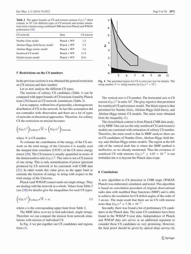
In Fig. 4 we put together our CS candidates and regionsfrom (1).

Fig. 4 The permitted region for CS to exist (see text for details). Thestring number N vs. string tension (in Gμ/c2 × 107)

The vertical axis is CS number. The horizontal axis is CStension Gμ/c2 in units 107. The gray region is that permittedfor semilocal CS and textures model. The black region is thatpermitted for Nambu–Goto, Abelian-Higgs field theory, andAbelian-Higgs mimic CS models. The areas were obtainedfrom the inequality (1).

The closed black contour is from Planck CMB data analy-sis by MHF. One can see the only semilocal CS (and textures)models are consistent with estimation of solitary CS number.Therefore, the main result is that in MHF analysis there areno CS candidates of Nambu–Goto, Abelian-Higgs field the-ory, and Abelian-Higgs mimic models. The region at the leftside of the vertical dash line is where the MHF method isineffective, as we already mentioned. Thus the existence ofsemilocal CS with tensions Gμ/c2 ≤ 4.83 × 10−7 is notforbidden but it is beyond the Planck data scope.

6 Conclusions

A new algorithm to CS detection in CMB maps (WMAP,Planck) was elaborated, simulated, and tested. This algorithmis based on convolution procedure of original observationalradio data with modified Haar functions (MHF) and is ableto achieve the resolution for CS deficit angles of the order of1 arcsec. The main result that there are no CS with tensionmore than Gμ/c2 = 7.36 × 10−7.

Secondly, there was found a list of preliminary CS candi-dates in the Planck data. The same CS candidates have beenfound in the WMAP 9-year data. Independence of Planckand WMAP data sets serves as an additional argument toconsider those CS candidates as very promising. However,the final proof should be given by optical deep surveys by

123


observation of gravitational lensing chains (this is the aim offuture intense work).

Finally, our MHF algorithm with the results in [18] madeit possible to clarify the preferred CS types. The most prefer-able types of CS are semilocal ones, described by the modelwith complex scalar doublet [14]. If its imaginary part isequal to 0, the semilocal CS becomes the Abelian-Higgs CS.The main difference between these two types of CS is that thesemilocal CS can have ends (monopoles) and can be unsta-ble under certain conditions. The topological (“ordinary”)CS have no ends. Formally they break on the surface of lastscattering. It means that if our CS candidates are topologicaldefects, then they have to be very far from the observer, upto z = 7, because their length is much less than 100◦ [13].In this case we have no possibility to observe their effectsin the optical data by looking through gravitational lensingevents, and we will never confirm our candidates by inde-pendent optical observation. But the situation substantiallychanges if we are dealing with semilocal CS. They can becloser to us, being not very long. Therefore our strategy isnow to find suitable optical fields to search for the chainsof gravitational lenses, produced by candidates to semilocalCS. The structure of the CS candidates found by the MHFmethod confirms the view of semilocal CS as a collection ofsegments. It is also necessary to mention that the compar-isons with the data for the search of non-Gaussian signals[18] shows that the presence of several (up to 3) Nambu–Goto CS is also possible but the semilocal CS remain themost favored.

Acknowledgments We are very grateful to Prof. M. Capaccioli fordiscussion. The support by the grant “Messaggeri della conoscescenza”of the Italian Ministry of University and Research is acknowledged.

Open Access This article is distributed under the terms of the CreativeCommons Attribution License which permits any use, distribution, andreproduction in any medium, provided the original author(s) and thesource are credited.Funded by SCOAP3 / License Version CC BY 4.0.

Appendix I: Modified Haar functions with cyclic shift

According to general theorems for Euclidean spaces, in spaceL2 there are complete orthogonal systems of functions.

Any function g(x) belonging to the space L2 can be rep-resented as a sum of Fourier series on a system of functionsfi (x):

g(x) =∞∑

i=1

ci fi (x).

Here ci are Fourier coefficients of the function g(x) on thesystem fi (x):

ci = 1

‖ fi‖2

∫g(x) fi (x)dμ,

where

‖ fi‖2 =∫

fi (x)2dμ.

By Haar [22] has been introduced a set of functions, com-plete and orthonormal on the space [0, 1]. This system hasbeen defined by the function

φ0 = 1

and by the set of functions (“series” of functions):

φ0 1

φ1 1, φ1 2

φ2 1, φ2 2, φ2 3, φ2 4

. . .

φn 1, φn 2, φn 3, . . . , φn 2n .

The “series” number n refers to 2n functions. We have

φ0 1 ={

1, 0 < x < 1/2,

−1, 1/2 < x < 1,

φ1 1 =

⎧⎪⎪⎨

⎪⎪⎩

√2, 0 < x < 1/4,

−√2, 1/4 < x < 1/2,

0, 1/2 < x < 1,

φ1 2 =

⎧⎪⎪⎨

⎪⎪⎩

0, 0 < x < 1/2,√

2, 1/2 < x < 3/4,

−√2, 3/4 < x < 1.

In points of discontinuity the Haar functions φn, i can bedefined arbitrarily. In the common case:

φ0 = 1

φn i =

⎧⎪⎪⎪⎪⎪⎨

⎪⎪⎪⎪⎪⎩

2n2 ,

i − 1

2n< x <

i − 1

2n+ 1

2n+1 ,

−2n2 ,

i − 1

2n+ 1

2n+1 < x <i

2n,

0, x /∈[

i − 1

2n; i

2n

],

n = 0, 1, . . . ; i = 1, 2, . . . , 2n .

Let us introduce the modified Haar functions {ψn i } withcyclic shift [23]. For simplicity we will take them on thecompact space [0, 1] with a real cyclic shift a ∈ [0, 1/2].Depending on the parameter a the functions {ψn i } can bedivided into four similar groups for 0 < a < 1 − i/2n ,1 − i/2n < a < 1 − i/2n + 1/2n+1, 1 − i/2n + 1/2n+1 <

a < 1 − i/2n + 1/2n , and 1 − (i − 1)/2n < a < 1/2.The subscripts “0” and “1” refer to the radial and angular

variables of a CS, respectively.

123


For the first case we have

ψ(a)n i =

⎧⎪⎪⎪⎪⎪⎪⎨

⎪⎪⎪⎪⎪⎪⎩

2n2 ,

i − 1

2n+ a < x <

i − 1

2n+ a + 1

2n+1 ,

−2n2 ,

i − 1

2n+ a + 1

2n+1 < x <i

2n+ a,

0, x /∈[

i − 1

2n+ a; i

2n+ a

].

If 1 − i/2n < a < 1 − i/2n + 1/2n+1, then

ψ(b)n i =

⎧⎪⎪⎪⎪⎪⎪⎪⎪⎪⎪⎨

⎪⎪⎪⎪⎪⎪⎪⎪⎪⎪⎩

2n2 ,

i − 1

2n+ a < x <

i − 1

2n+ a + 1

2n+1 ,

−2n2 ,

i − 1

2n+ a + 1

2n+1 < x < 1⋃

0 < x <i

2n+ a − 1,

0, x ∈[

i

2n+ a − 1; i − 1

2n+ a

].

If 1 − i/2n + 1/2n+1 < a < 1 − i/2n + 1/2n , then

ψ(c)n i =

⎧⎪⎪⎪⎪⎪⎪⎪⎪⎪⎪⎨

⎪⎪⎪⎪⎪⎪⎪⎪⎪⎪⎩

2n2 ,

i − 1

2n+ a < x < 1

⋃0

< x <i − 1

2n+ a + 1

2n+1 − 1,

−2n2 ,

i −1

2n+a+ 1

2n+1 −1 < x <i

2n+ a − 1,

0, x ∈[

i

2n+ a − 1; i − 1

2n+ a

].

If 1 − (i − 1)/2n < a < 1/2, then

ψ(d)n i =

⎧⎪⎪⎪⎪⎪⎨

⎪⎪⎪⎪⎪⎩

2n2 ,

i − 1

2n+a−1 < x <

i − 1

2n+a−1+ 1

2n+1 ,

−2n2 ,

i − 1

2n+a−1+ 1

2n+1 < x <i

2n+a − 1,

0, x /∈[

i − 1

2n+ a − 1; i

2n+ a − 1

].

For fixed a the set of modified Haar functions is completeand orthonormal, as well as the system of classical Haar func-tions [23]. Therefore it is correct to use it in searching forsignals.

Appendix II: Simulations of false string detection

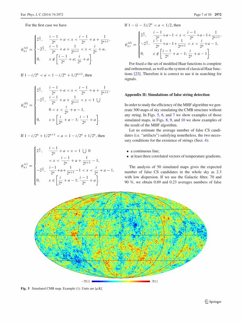
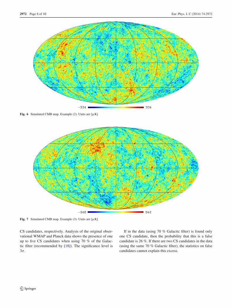
In order to study the efficiency of the MHF algorithm we gen-erate 300 maps of sky simulating the CMB structure withoutany string. In Figs. 5, 6, and 7 we show examples of thosesimulated maps, in Figs. 8, 9, and 10 we show examples ofthe result of the MHF algorithm.

Let us estimate the average number of false CS candi-dates (i.e. “artifacts”) satisfying nonetheless, the two neces-sary conditions for the existence of strings (Sect. 4):

• a continuous line;• at least three correlated vectors of temperature gradients.

The analysis of 50 simulated maps gives the expectednumber of false CS candidates in the whole sky as 2.3with low dispersion. If we use the Galactic filter, 70 and90 %, we obtain 0.69 and 0.23 averages numbers of false

Fig. 5 Simulated CMB map. Example (1). Units are [µK]

123




CS candidates, respectively. Analysis of the original obser-vational WMAP and Planck data shows the presence of oneup to five CS candidates when using 70 % of the Galac-tic filter (recommended by [18]). The significance level is3σ .

If in the data (using 70 % Galactic filter) is found onlyone CS candidate, then the probability that this is a falsecandidate is 26 %. If there are two CS candidates in the data(using the same 70 % Galactic filter), the statistics on falsecandidates cannot explain this excess.

123


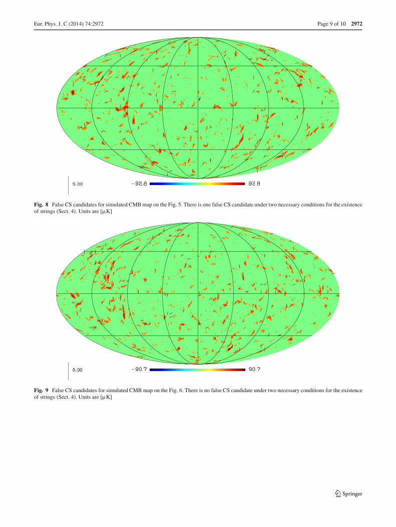
Fig. 8 False CS candidates for simulated CMB map on the Fig. 5. There is one false CS candidate under two necessary conditions for the existenceof strings (Sect. 4). Units are [µK]

Fig. 9 False CS candidates for simulated CMB map on the Fig. 6. There is no false CS candidate under two necessary conditions for the existenceof strings (Sect. 4). Units are [µK]

123


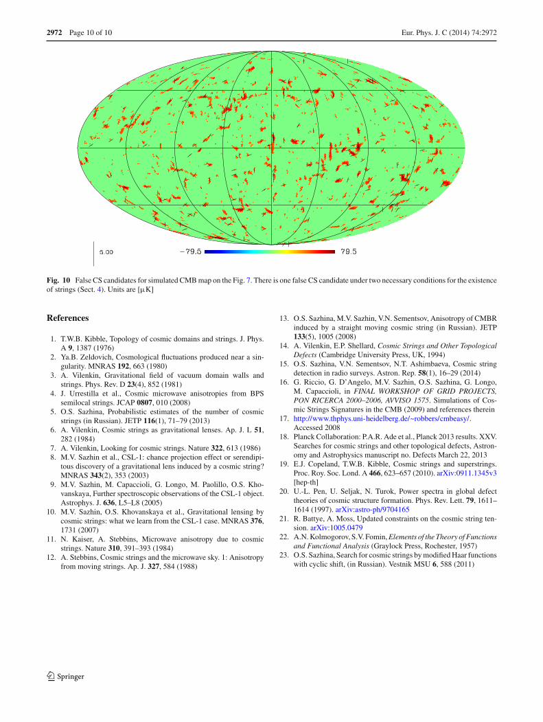
Fig. 10 False CS candidates for simulated CMB map on the Fig. 7. There is one false CS candidate under two necessary conditions for the existenceof strings (Sect. 4). Units are [µK]

References

1. T.W.B. Kibble, Topology of cosmic domains and strings. J. Phys.A 9, 1387 (1976)

2. Ya.B. Zeldovich, Cosmological fluctuations produced near a sin-gularity. MNRAS 192, 663 (1980)

3. A. Vilenkin, Gravitational field of vacuum domain walls andstrings. Phys. Rev. D 23(4), 852 (1981)

4. J. Urrestilla et al., Cosmic microwave anisotropies from BPSsemilocal strings. JCAP 0807, 010 (2008)

5. O.S. Sazhina, Probabilistic estimates of the number of cosmicstrings (in Russian). JETP 116(1), 71–79 (2013)

6. A. Vilenkin, Cosmic strings as gravitational lenses. Ap. J. L 51,282 (1984)

7. A. Vilenkin, Looking for cosmic strings. Nature 322, 613 (1986)8. M.V. Sazhin et al., CSL-1: chance projection effect or serendipi-

tous discovery of a gravitational lens induced by a cosmic string?MNRAS 343(2), 353 (2003)

9. M.V. Sazhin, M. Capaccioli, G. Longo, M. Paolillo, O.S. Kho-vanskaya, Further spectroscopic observations of the CSL-1 object.Astrophys. J. 636, L5–L8 (2005)

10. M.V. Sazhin, O.S. Khovanskaya et al., Gravitational lensing bycosmic strings: what we learn from the CSL-1 case. MNRAS 376,1731 (2007)

11. N. Kaiser, A. Stebbins, Microwave anisotropy due to cosmicstrings. Nature 310, 391–393 (1984)

12. A. Stebbins, Cosmic strings and the microwave sky. 1: Anisotropyfrom moving strings. Ap. J. 327, 584 (1988)

13. O.S. Sazhina, M.V. Sazhin, V.N. Sementsov, Anisotropy of CMBRinduced by a straight moving cosmic string (in Russian). JETP133(5), 1005 (2008)

14. A. Vilenkin, E.P. Shellard, Cosmic Strings and Other TopologicalDefects (Cambridge University Press, UK, 1994)

15. O.S. Sazhina, V.N. Sementsov, N.T. Ashimbaeva, Cosmic stringdetection in radio surveys. Astron. Rep. 58(1), 16–29 (2014)

16. G. Riccio, G. D’Angelo, M.V. Sazhin, O.S. Sazhina, G. Longo,M. Capaccioli, in FINAL WORKSHOP OF GRID PROJECTS,PON RICERCA 2000–2006, AVVISO 1575. Simulations of Cos-mic Strings Signatures in the CMB (2009) and references therein

17. http://www.thphys.uni-heidelberg.de/~robbers/cmbeasy/.Accessed 2008

18. Planck Collaboration: P.A.R. Ade et al., Planck 2013 results. XXV.Searches for cosmic strings and other topological defects, Astron-omy and Astrophysics manuscript no. Defects March 22, 2013

19. E.J. Copeland, T.W.B. Kibble, Cosmic strings and superstrings.Proc. Roy. Soc. Lond. A 466, 623–657 (2010). arXiv:0911.1345v3[hep-th]

20. U.-L. Pen, U. Seljak, N. Turok, Power spectra in global defecttheories of cosmic structure formation. Phys. Rev. Lett. 79, 1611–1614 (1997). arXiv:astro-ph/9704165

21. R. Battye, A. Moss, Updated constraints on the cosmic string ten-sion. arXiv:1005.0479

22. A.N. Kolmogorov, S.V. Fomin, Elements of the Theory of Functionsand Functional Analysis (Graylock Press, Rochester, 1957)

23. O.S. Sazhina, Search for cosmic strings by modified Haar functionswith cyclic shift, (in Russian). Vestnik MSU 6, 588 (2011)

123

http://www.thphys.uni-heidelberg.de/~robbers/cmbeasy/

http://arxiv.org/abs/0911.1345v3

http://arxiv.org/abs/astro-ph/9704165

http://arxiv.org/abs/1005.0479

Documents

Observational constraints on the types of cosmic strings