1

Objectively combining AR5 instrumental period and

paleoclimate climate sensitivity evidence

Nicholas Lewis1

Bath, United Kingdom

Peter Grünwald2

CWI Amsterdam and Leiden University, the Netherlands

Reformatted version (incorporating proof-reading corrections) of

manuscript accepted on 28 May 2017 for publication in Climate Dynamics,

The final publication will be available at Springer via http://dx.doi.org/[DOI not yet known]

1 Corresponding author address: Bath, United Kingdom.

E-mail: nhlewis@btinternet.com

2 E-mail: pdg@cwi.nl

2

Abstract

Combining instrumental period evidence regarding equilibrium climate sensitivity with largely

independent paleoclimate proxy evidence should enable a more constrained sensitivity estimate to be

obtained. Previous, subjective Bayesian approaches involved selection of a prior probability

distribution reflecting the investigators' beliefs about climate sensitivity. Here a recently developed

approach employing two different statistical methods – objective Bayesian and frequentist likelihood-

ratio – is used to combine instrumental period and paleoclimate evidence based on data presented and

assessments made in the IPCC Fifth Assessment Report. Probabilistic estimates from each source of

evidence are represented by posterior probability density functions (PDFs) of physically-appropriate

form that can be uniquely factored into a likelihood function and a noninformative prior distribution.

The three-parameter form is shown accurately to fit a wide range of estimated climate sensitivity

PDFs. The likelihood functions relating to the probabilistic estimates from the two sources are

multiplicatively combined and a prior is derived that is noninformative for inference from the

combined evidence. A posterior PDF that incorporates the evidence from both sources is produced

using a single-step approach, which avoids the order-dependency that would arise if Bayesian updating

were used. Results are compared with an alternative approach using the frequentist signed root

likelihood ratio method. Results from these two methods are effectively identical, and provide a 5-95%

range for climate sensitivity of 1.1–4.05 K (median 1.87 K).

3

1. Introduction

Equilibrium climate sensitivity (ECS) – the rise in global mean surface temperature (GMST) resulting

from a doubling of atmospheric carbon dioxide (CO2) concentration, once the ocean has reached

equilibrium – is a key climate system parameter. Effective radiative forcing (ERF) provides a metric,

designed to be a good indicator of their impact on GMST, of the effects on the Earth's radiative

imbalance of changes in CO2, in other radiatively-active gases and in other drivers of climate change.

For changes between equilibrium states, ECS may then be estimated as the ratio of the change in

GMST (ΔT) to the change (ΔFn) in ERF normalised by division by the ERF from a doubling of CO2

concentration: nECS /T F .

It has proved difficult to narrow uncertainty about ECS, given observational data limitations

and internal climate system variability. It may be possible better to constrain ECS by combining

probabilistic evidence from different sources. Several authors have sought to do so (Hegerl et al. 2006;

Annan and Hargreaves 2006; Aldrin et al. 2012; Stevens et al. 2016) using subjective Bayesian

methods, however their results were significantly influenced by the initial prior distributions they

chose. Here we apply a recently established method of combining evidence with differing

characteristics to generate an ECS estimate based on instrumental and paleoclimate evidence. That

evidence, formulated as probability density functions (PDFs), is derived from estimates presented in

the IPCC Fifth Assessment Working Group 1 Report (AR5). The results themselves are considered to

be of some importance since they are intended to reflect carefully considered assessments in AR5, but

an equally important motivation is bringing a more objective method of combining evidence regarding

ECS and similar parameters to the attention of the climate science community.

Before going further, let us clarify the scope of our study. We study ECS, and not Earth system

sensitivity (ESS) – the GMST increase from a doubling of CO2 concentration once slow climate

system components such as the cryosphere and vegetation have equilibrated as well as the atmosphere

and ocean. Recently, using proxy data for the past 800 kyr, Snyder (2016) estimated a 7–13 K range

for ESS. However, using data from the same period Palaeosens Project Members (2012) estimated ESS

to be 3.4 times as high as ECS. Since ESS is by definition a quite different notion of climate sensitivity

from ECS we will not consider it here.

We use both “objective Bayesian” and frequentist likelihood-ratio statistical methods, and

show that these approaches yield results which are almost identical to each other, but very different

from those obtained with a subjective Bayesian method when employing a uniform prior; this

commonly used prior is in this instance unintentionally highly informative (inference using it is not

dominated by the data involved). Objective Bayesian methods (Berger 2006, Bernardo 2009), which

use 'noninformative' priors, are an integral and thriving part of Bayesian statistics (a substantial

fraction of papers at the main Bayesian (ISBA) meetings are dedicated to ‘objective Bayes’).

Nevertheless, they are not often employed within the climate science community and since some sort

of subjectivity is inevitable in any statistical analysis, if only regarding the chosen model, some

discussion is warranted as to what is precisely meant by ‘objective’ and 'noninformative' here; we defer

this discussion to Section 2.2.

A key attraction of combining a single instrumental period and a single paleoclimate evidence

source regarding ECS is that, unlike when combining evidence from, e.g., different sources from

within the instrumental period, sources of error should be largely independent; this greatly simplifies

the statistical inference. Our results thus combine a single instrumental period source with a single

paleoclimate source. In our main result, the instrumental period source is taken from Lewis and Curry

(2015); for comparison, we provide a second result in which the instrumental period source is taken

from Otto et al. (2013), a study in which many AR5 lead authors were involved. The paleoclimate

4

source is the same in both results, representing a summary of the expert assessment made in AR5 and

of studies cited in it. Below we first describe our methodology and then the sources of evidence in

more detail.

1.1 Methodology and Overview

Standard objective Bayesian methodology, reviewed in Section 2, requires the evidence to be

represented as a likelihood, i.e. the probability density of observed data as a function of parameters in

the assumed statistical model (a "statistical model" meaning a family of probability distributions). In

our case, however, the evidence is of a different form: the two instrumental period sources provide a

probability density function (PDF) for the single parameter θ (ECS) of interest, while the paleoclimate

source provides a partial specification of such a PDF. From a Bayesian perspective we may view these

PDFs as ‘posteriors’ arising from some data (likelihood) and prior. We somehow need to construct the

required likelihoods based on the given PDFs. To this end, we assume a ratio-normal model, which

(Section 3.1) is a physically appropriate model to use in this case, both for instrumental and

paleoclimate evidence. Combining the ratio-normal model with its corresponding objective Bayesian

prior leads to a posterior distribution on ECS that is severely constrained in form: it is fully determined

by three parameters. Raftery and Schweder (1993; henceforth RS 93) provided a remarkably accurate

analytic approximation of the posterior for a parameter that is the ratio of two other parameters whose

joint posterior is bivariate normal, which (Section 3.1) corresponds to both of them being location

parameters estimated with normal error and using a noninformative uniform prior. We henceforth call

this the ‘RS93 posterior’. (A location parameter is one where the probability density of an observed

datum depends only on the error – the difference between the datum and parameter values.) The two

location parameters may be scaled equally without affecting the distribution of their ratio; it is

convenient to scale so that the denominator distribution has a unit mean. The distribution of their ratio

is therefore specified by three parameters, provided the numerator and denominator errors are

independent: the mean of the scaled numerator distribution and the standard deviations of the scaled

numerator and denominator distributions. The same three parameters specify the approximating RS93

posterior. By adjusting these three parameters, the RS93 posterior can be made to fit published PDFs

for ECS very well: not just the two instrumental-period PDFs used for our main results, but, as we

show in Section 3.2, also a wide range of variously shaped PDFs obtained by other authors. While the

original PDFs were not directly given in the RS93 form, we do take this as evidence that the ratio-

normal model is indeed appropriate, and that sound published PDFs for ECS can be legitimately

viewed as (the RS 93 approximation to) posteriors arising from data and an objective (noninformative)

prior for the ratio-normal model. As shown by Lewis (in press), the RS93 posterior induces a unique

factorization into a likelihood and (noninformative) prior, giving us the desired likelihood needed for

our objective Bayesian approach.

While in the paleoclimate case there is no published PDF that appears to be representative of

the evidence in AR5, combining the range assessed in AR5 with a median estimate from studies it cites

provides sufficient information to uniquely fit an RS93 posterior, again leading to the desired

likelihood. Below we explain how this fitting process faithfully represents paleoclimate evidence.

Both our results thus combine two likelihoods, induced by RS93 posterior PDFs, using an

objective Bayesian approach. The obvious but incorrect way to do this is to copy the subjective

Bayesian updating method (using the posterior based on the first source as the prior for the second).

However, as explained in section 2.2, this leads to anomalies such as order dependence (Seidenfeld

1979, Kass and Wasserman 1996), since the noninformative prior for the first likelihood is in general

different from the noninformative prior for the second likelihood; moreover, as shown by Lewis (in

press), it has quite bad frequentist calibration properties. The ‘correct’ combination or updating

method, without such anomalies, was proposed by Lewis (2013b), and is also the method of choice

according to the information-theoretic Minimum Description Length method (Grünwald, 2007). The

5

details of applying such a method to RS93 ratio-normal approximation likelihoods were recently

worked out by Lewis (in press), who also shows that it enjoys much better frequency properties – we

review the method in Section 4.1 and 4.2. As a sanity check (Section 4.3), we also use a purely

frequentist combination method and find that it gives near-identical results, in the sense that it gives

rise to confidence intervals that almost precisely match our objective-Bayesian credible intervals.

Section 5 then presents these results, which are summarized in Figure 3.

In the remainder of this introduction, we shall further motivate our particular choice for the two

instrumental period sources as well as our single paleoclimate source, itself a summary of various

sources represented in the AR5 expert assessment.

1.2 Instrumental Period Evidence

AR5 cited a large number of instrumental period ECS estimates that gave widely varying best

estimates and uncertainty ranges, but expressed [Section 12.5.3] doubts about estimates based on short

timescales or non-greenhouse gas forcings. The AR5 authors evidently considered that estimates based

on longer-term greenhouse gas-dominated warming over the instrumental period should be more

reliable: AR5 attributes its reduction in the bottom of the likely range for ECS to estimates using

multidecadal data from the instrumental period, stating [Box 12.2] that the reduction "reflects the

evidence from new studies of observed temperature change, using the extended records in atmosphere

and ocean". Here, rather than using some average of instrumental period ECS estimates cited in AR5,

we focus on estimation that conforms with the assessment in AR5 of the relative merits of different

approaches and reflects AR5 values for radiative forcings and heat uptake, its reassessment of

uncertain aerosol forcing being particularly relevant. One important such estimate was provided by

Otto et al. (2013, hereafter Oa13), a study in which many AR5 lead authors were involved. Oa13 was

an energy-budget study that reflected estimated changes in global surface temperature, forcing and

climate system heat uptake over the instrumental period, using a multimodel atmosphere-ocean general

circulation model (AOGCM)-derived estimate of forcing changes (with aerosol forcing adjusted).

Subsequent to the release of AR5, another energy budget ECS study (Lewis and Curry 2015, hereafter

LC15) used the updated estimates of forcing series from AR5, not available at the time of the Oa13

study, which differ from and have wider uncertainty ranges than those derived from AOGCMs. Like

Oa13, LC15 used the HadCRUT4 v2 global temperature dataset (Morice et al. 2012), AR5's

observationally-based estimate of recent heat accumulation in the climate system and a model-based

estimate of the small heat uptake early in the instrumental period. Its "preferred results" ECS estimate

is based on changes from 1859-1882 to 1995-2011, two periods with low volcanic activity and which

appear to have similar influences from internal variability. The distribution of ECS from those LC15

results is used as the most representative instrumental period evidence for this present study.

Comparative results using the best-constrained Oa13 ECS estimate (based on changes from 1860-1879

to 2000-2009) are also presented. That estimate has a slightly higher median than LC15's, principally

reflecting a greater estimate of the change in heat accumulation rate (LC15), but it is better

constrained, reflecting the narrower AOGCM-derived forcing uncertainty range.

1.3 Paleoclimate Evidence

Chapter 10 of AR5 concluded that uncertainties in paleoclimate estimates of ECS were likely to be

larger than for estimates from the instrumental record, since, as well as data uncertainties, feedbacks

could change between different climatic states.

Unlike for the instrumental evidence case, no single PDF has been published that fully

represents the evidence in and assessments of AR5. Instead, AR5 gives a probability range, based on

studies from various authors (Chylek and Lohmann 2008; Hargreaves and Annan 2012; Holden et al.

2010; Köhler et al. 2010; Palaeosens Project Members 2012; Schmittner et al. 2011; Schneider von

6

Deimling et al. 2006). To use our Bayesian combination method we first need to summarize this

information into a single RS93 posterior PDF, as explained above.

For this, we first recall AR5’s conclusion that paleoclimate evidence implied ECS was very

likely (90%+ probability) greater than 1 K and very likely less than 6 K, without giving any best

estimate. We treat that, conservatively, as implying a 10–90% (80%) range of 1–6 K. Whilst just a

range is sufficient to fit a symmetrical Gaussian probability distribution, it is insufficient to specify a

distribution in which the central tendency, dispersion and skewness are independent of each other. ECS

estimates are generally skewed, mainly reflecting uncertainty in the estimates of changes in forcings,

and their central tendency, dispersion and degree of skewness will vary from one estimate to another.

A RS93 posterior has three free parameters and provides independent control of these three

characteristics. To fit it to a given partially specified distribution thus requires, at a minimum, three

percentile points. Therefore, we first derive a median (50% percentile) paleoclimate estimate from all

the eight median estimates shown in the paleoclimate section of AR5 Figure 10.20b. Additionally, for

Chylek and Lohmann (2008) and Schneider von Deimling et al. (2006) (where only 5–95% ranges are

given) we take their midpoint as the median, there being no evidence of skewness in those studies'

results. We exclude Annan et al. (2005) as it provides no ECS lower limit. The mean and the median of

the ten median estimates are both marginally below 2.75 K. We round up and use 2.75 K as the median

ECS estimate from paleoclimate evidence.

Almost all the paleoclimate studies featured in AR5 Figure 10.20b focused on the well-studied

transition from Last Glacial Maximum (LGM) to preindustrial conditions. All but one of these LGM-

based studies estimated ECS for preindustrial conditions. They allowed for possible state dependence

of ECS by using climate models in which ECS was an emergent property that could vary with climate

state; the relationship between ECS for the LGM transition and ECS in preindustrial conditions varies

among climate models (Hargreaves et al. 2007; Otto-Bliesner et. al., 2009; Colman et al. 2009).

Recently, by regressing temperature against forcing over the warmest parts of glacial cycles during the

last 784 kyr, Friedrich et al. (2016) estimated ECS applying in preindustrial conditions as 4.9 K, well

above all the median estimates in AR5 Figure 10.20b. Their estimated 5.75 K warming and 6.5 Wm–2

forcing change for the LGM transition implies a lower energy-budget ECS estimate of 3.3K, in line

with the 3.2 K they derive from regressing temperature against forcing over complete glacial cycles

during the 784 kyr period. The high Friedrich et al. (2016) warm-climate ECS estimate may be more a

reflection of their temperature and forcing change estimates than of unusually strong estimated

climate-state dependence. Carefully constructed modern best estimates of the LGM transition

temperature change (4.0 K; Annan and Hargreaves 2013) and forcing change (9.5 Wm–2; Köhler et al.

2010) imply an energy budget LGM-transition ECS estimate of 1.6 K, half the Friedrich et al. (2016)

value. Moreover, regression plots of temperature against forcing in Martinez-Boti et al. (2015), using

data for both the 0-800 kyr and the late Plio-Pleistocene (2,300–3,300 kyr) periods, show little

evidence of higher sensitivity during the warmest parts of interglacials in the last 800 kyr or during the

even warmer late Plio-Pleistocene period, relative to that over the entire 0–800 kyr period.

Accordingly, we see no reason to revise upwards the 2.75 K median paleoclimate evidence ECS

estimate derived from paleoclimate studies shown in AR5 Figure 10.20b.

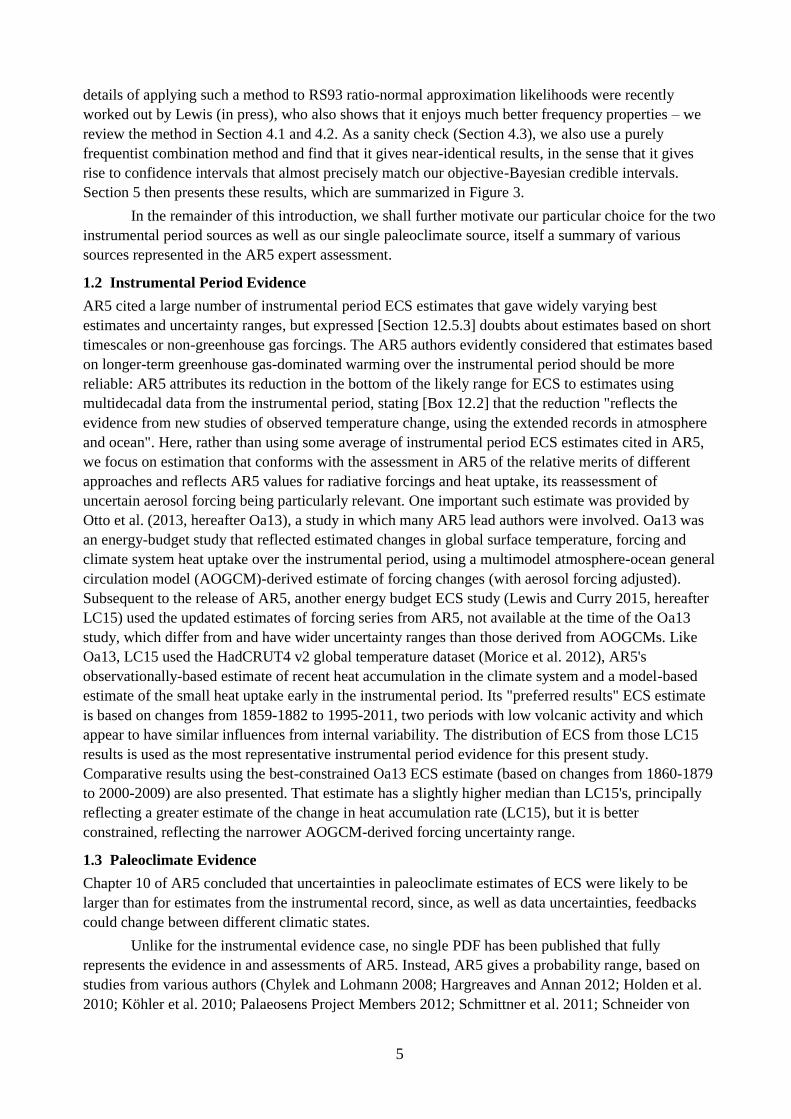
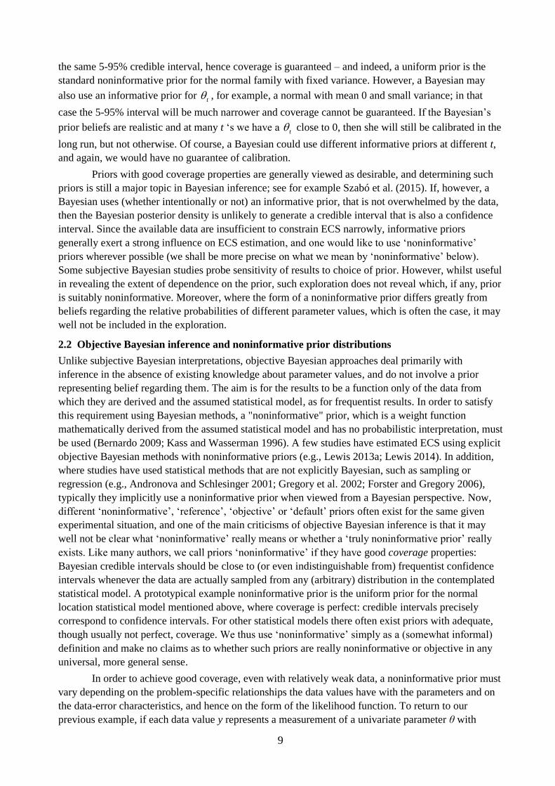
Figure 1 compares PDFs, medians and uncertainty ranges shown in AR5 Figure 10.20b, for

each of the paleoclimate studies it features, with the RS93 posterior which is based on a physically

appropriate model (see Section 3 for details), fitted to 10th, 50th and 90th percentiles of 1, 2.75 and 6

K. This distribution (black line), although not itself an IPCC assessment, is presented as fairly

representing the AR5 assessment from paleoclimate evidence of a 1–6 K uncertainty range for ECS,

treated conservatively as 10-90%, with a median consistent with those from studies featured in AR5.

The 17–83% range for the fitted RS93 posterior is 1.4–4.85 K. The fact that that range is only slightly

wider than the overall 'likely' (at least 66% probability) range of 1.5–4.5 K that AR5 derives in Chapter

7

10 from assessing all lines of observational evidence combined supports treating the 1–6 K range as

covering only the central 80% probability. So also does the lack of a high confidence appraisal being

given to the paleoclimate range in AR5.

Figure 1. Estimated PDFs for individual paleoclimate studies compared with the distribution fitted to

the AR5 paleoclimate range. The thick black line shows the distribution used to represent the AR5 1–6

K paleoclimate range, treated as representing 10–90% probability and as having a median of 2.75 K.

The thin colored lines show PDFs for the paleoclimate studies featured in Figure 10.20b of AR5, fitted

by Gaussian distributions to their ranges in the case of Chylek and Lohmann (2008) (blue line) and

Schneider von Deimling et al (2006) (cyan line) and otherwise as plotted in AR5 Figure 10.20b.

Although Chylek and Lohmann's estimate is a 95% range, since AR5 assesses its true uncertainty as

likely larger, the range is treated here as being 5–95% and a PDF based on treating it as a 17–83% range

is also shown (dashed blue line). Secondary estimates (shown dashed or dashed-dotted in Figure 10.20b

of AR5) are not plotted but were included when determining the median of the distribution used to

represent the AR5 paleoclimate range,. The box plots indicate boundaries for the percentiles 5–95

(vertical bar at ends), 17–83 (box-ends), and 50 (vertical bar in box).

The rest of this paper is organized as follows. Section 2 considers statistical parameter

inference methods. Section 3 deals with selecting a suitable form of parameterized standard

distribution to match ECS estimates and with fitting the form selected. Section 4 deals with likelihoods

and noninformative priors corresponding to the fitted PDFs and the combined evidence that they

provide. Section 5 presents results, and Section 6 discusses issues raised.

2. Statistical inference methodology

2.1 Subjective Bayesian inference and calibration of Bayesian probabilities

In the continuous case, from Bayes theorem (Bayes 1763) we can state conventionally that the

(posterior) PDF, |p y , for a parameter (vector) θ on which observed data y depend, is

proportional to the probability density of the data |py

y (called the likelihood function, or just the

8

likelihood, denoted by ( )L , when considered as a function of θ, with y fixed) multiplied by the

density of a prior distribution (prior) for θ, p :

( | ) ( | ) ( )p p py

y y (1)

(the subscripts indicating which variable density is for). The constant of proportionality is ascertainable

since the posterior PDF must integrate to unit probability. Under subjective Bayesian interpretations,

the prior (and hence the posterior) represent the investigator's degree of belief regarding possible

parameter values; the prior and posterior reflect respectively relevant prior knowledge and that

knowledge updated by the observed data. Both prior and posterior are personal to the investigator.

Bayesian credible intervals – i.e. uncertainty intervals taken from percentile points of the

posterior cumulative distribution function (CDF) – and frequentist confidence intervals involve

conceptually different kinds of probability, respectively epistemic (relating to knowledge) and aleatory

(random) probabilities. However, to avoid Bayesian inference giving misleading results it is necessary

that a prior be used that provides correct calibration of posterior probabilities to frequencies, at least

approximately (Fraser et al. 2010). To explain this in more detail, consider a research center where

every month a new experimental study is performed both by a Bayesian and a frequentist statistician.

Each month ( 1,2, , )t t m they are given a new data set, unrelated to any previous data set,

involving a parameter t , and they agree on an appropriate statistical model for the data set. (To

simplify the picture, we could also imagine, less realistically, that all the data sets refer to the same

statistical model and the same parameter t – the story below is valid irrespective of whether the data

sets come from the same physical source or not.) They then analyze the data separately. The Bayesian

outputs a 5-95% credible interval [ , ]t ta b . This means she believes that the true parameter value, t ,

for the t-th data set is contained in [ , ]t ta b with (epistemic) probability 90%; more specifically, it is

smaller than ta with probability 5%, and larger than tb with probability 5%. The frequentist outputs a

5-95% confidence interval [ , ]t tc d . Such confidence intervals are constructed such that, no matter what

the true parameter value t is, the probability that it will be contained in [ , ]t tc d is 90%, with a 5%

probability of it being below tc and a 5% probability of it being above td . These are aleatory

probabilities, deriving from randomness in the data values. As a result, the frequentist is guaranteed to

be (long-run) calibrated: in the long run (for large m), about 90% of the intervals he outputs will

contain the true parameter value. On the other hand, whether the Bayesian's credible interval in month t

is really a confidence interval in the frequentist sense depends on the prior she uses in month t. If she

uses an informative prior, then this expresses a belief that certain parameter values are more likely than

others, and if these beliefs are wrong then her credible interval in month t will not be a confidence

interval; and if this happens at many t then she will not be calibrated. We say that coverage holds for

Bayesian estimation (for a single experiment, e.g. at a particular t) if the credible interval it produces is

also (approximately) a confidence interval. For most common single-parameter statistical models, there

exist priors which guarantee this: use of a suitably noninformative prior will result in posterior PDFs

and related credible intervals that at least approximately equate to confidence intervals (Bernardo

2009) and hence satisfy coverage. If a Bayesian always (at each t) uses priors guaranteeing coverage,

then she is guaranteed to be calibrated in the long run.

As an example, consider a simplified case where in each month t, the statisticians obtain a

sample of length nt from a normal distribution with unknown mean t and variance 1; denote the

sample mean by ˆt . The standard 5-95% confidence interval for this model is the interval

ˆ ˆ[ , ]t t t tf f , where 1.96t tf n . A Bayesian who uses a uniform prior on t will output exactly

9

the same 5-95% credible interval, hence coverage is guaranteed – and indeed, a uniform prior is the

standard noninformative prior for the normal family with fixed variance. However, a Bayesian may

also use an informative prior for t , for example, a normal with mean 0 and small variance; in that

case the 5-95% interval will be much narrower and coverage cannot be guaranteed. If the Bayesian’s

prior beliefs are realistic and at many t ‘s we have a t close to 0, then she will still be calibrated in the

long run, but not otherwise. Of course, a Bayesian could use different informative priors at different t,

and again, we would have no guarantee of calibration.

Priors with good coverage properties are generally viewed as desirable, and determining such

priors is still a major topic in Bayesian inference; see for example Szabó et al. (2015). If, however, a

Bayesian uses (whether intentionally or not) an informative prior, that is not overwhelmed by the data,

then the Bayesian posterior density is unlikely to generate a credible interval that is also a confidence

interval. Since the available data are insufficient to constrain ECS narrowly, informative priors

generally exert a strong influence on ECS estimation, and one would like to use ‘noninformative’

priors wherever possible (we shall be more precise on what we mean by ‘noninformative’ below).

Some subjective Bayesian studies probe sensitivity of results to choice of prior. However, whilst useful

in revealing the extent of dependence on the prior, such exploration does not reveal which, if any, prior

is suitably noninformative. Moreover, where the form of a noninformative prior differs greatly from

beliefs regarding the relative probabilities of different parameter values, which is often the case, it may

well not be included in the exploration.

2.2 Objective Bayesian inference and noninformative prior distributions

Unlike subjective Bayesian interpretations, objective Bayesian approaches deal primarily with

inference in the absence of existing knowledge about parameter values, and do not involve a prior

representing belief regarding them. The aim is for the results to be a function only of the data from

which they are derived and the assumed statistical model, as for frequentist results. In order to satisfy

this requirement using Bayesian methods, a "noninformative" prior, which is a weight function

mathematically derived from the assumed statistical model and has no probabilistic interpretation, must

be used (Bernardo 2009; Kass and Wasserman 1996). A few studies have estimated ECS using explicit

objective Bayesian methods with noninformative priors (e.g., Lewis 2013a; Lewis 2014). In addition,

where studies have used statistical methods that are not explicitly Bayesian, such as sampling or

regression (e.g., Andronova and Schlesinger 2001; Gregory et al. 2002; Forster and Gregory 2006),

typically they implicitly use a noninformative prior when viewed from a Bayesian perspective. Now,

different ‘noninformative’, ‘reference’, ‘objective’ or ‘default’ priors often exist for the same given

experimental situation, and one of the main criticisms of objective Bayesian inference is that it may

well not be clear what ‘noninformative’ really means or whether a ‘truly noninformative prior’ really

exists. Like many authors, we call priors ‘noninformative’ if they have good coverage properties:

Bayesian credible intervals should be close to (or even indistinguishable from) frequentist confidence

intervals whenever the data are actually sampled from any (arbitrary) distribution in the contemplated

statistical model. A prototypical example noninformative prior is the uniform prior for the normal

location statistical model mentioned above, where coverage is perfect: credible intervals precisely

correspond to confidence intervals. For other statistical models there often exist priors with adequate,

though usually not perfect, coverage. We thus use ‘noninformative’ simply as a (somewhat informal)

definition and make no claims as to whether such priors are really noninformative or objective in any

universal, more general sense.

In order to achieve good coverage, even with relatively weak data, a noninformative prior must

vary depending on the problem-specific relationships the data values have with the parameters and on

the data-error characteristics, and hence on the form of the likelihood function. To return to our

previous example, if each data value y represents a measurement of a univariate parameter θ with

10

random error ε having a normal distribution with mean 0 and variance 1 (so that the data value itself is

normally distributed with mean θ and variance 1) then the likelihood is proportional to 2exp[ ( ) / 2]y . As we saw before, in this case a uniform prior is noninformative for inference

about θ. On the other hand, if the data value represents a measurement of the cube of θ , then the

likelihood function is proportional to 3 2exp[ ( ) / 2]y , and it turns out that to be noninformative the

prior must be proportional to 2 . Noninformative priors for parameters therefore vary with the

experiment involved. Accordingly, if two studies estimating the same parameter using data from

different experiments involve different likelihood functions, as is likely, they will give rise to different

noninformative priors. This might appear to militate against using objective Bayesian methods to

combine evidence in such cases. Using the appropriate, individually noninformative, prior, standard

Bayesian updating would, inconsistently, produce a different result according to the order in which

Bayes' theorem was applied to the two datasets (Kass and Wasserman 1996). While this fact has been

used to criticize objective Bayes methods (Seidenfeld 1979), the issue can be avoided by applying

Bayes theorem once only, to the joint likelihood function for the combination of the instrumental

period and paleoclimate estimates, with a single noninformative prior being computed for inference

therefrom, as was proposed by Lewis (2013b). It is also the proper way to proceed according to the

Minimum Description Length Principle, an alternative approach to statistics that has its roots in

information theory and data compression (Grünwald 2007, Chapter 11, Section 11.4.2), and it is the

method that will be followed in this paper.

The first general method for computing noninformative priors (Jeffreys 1946) was devised

using invariance arguments. Jeffreys prior is the square root of the (expected) Fisher information, or of

its determinant where the parameter is a vector. Fisher information – the expected value of the negative

second derivative of the log-likelihood function with respect to the parameters upon which the

probability of the data depend – measures the amount of information that the data carries, averaged

across possible data values, about unknown parameters at varying values thereof. Inference using a

Jeffreys prior is invariant under transformations of parameter and/or data variables, a highly desirable

characteristic. In the normal location family example above, Jeffreys’ prior coincides with the uniform

prior.

Reference analysis (Bernardo 1979; Berger and Bernardo 1992), which involves maximizing

the (expected value of) missing information about the parameters of interest, is usually regarded as the

gold-standard for objective Bayesian inference, as reference priors have the least influence on

inference relative to the data, where ‘influence’ is measured in an information-theoretic sense.

Reference analysis may be argued to provide an “objective” Bayesian solution to statistical inference

problems in just the same sense that conventional statistical methods claim to be “objective”: in that

the solutions only depend on model assumptions and observed data (Bernardo 2009). In the univariate

parameter continuous case, as here, Jeffreys prior is normally the reference prior, and it provides

credible intervals that are closer to confidence intervals than with any other prior (Welch and Peers

1963; Hartigan 1965) – thus being noninformative in exactly the sense we desire.

2.3 Likelihood-ratio inference

Another way of objectively combining probabilistic evidence regarding ECS from two independent

sources is to use frequentist likelihood-ratio methods, which directly provide estimated confidence

intervals. A profile likelihood may be used when there are nuisance parameters to eliminate. The

likelihood ratio is the ratio, at each parameter value, of the likelihood there to the maximum likelihood

at any parameter value. Equivalently, it is the likelihood normalised to a maximum value of one.

Likelihood-ratio methods are based on asymptotic normal approximations and produce frequentist

confidence intervals that are exact only when the underlying distributions are normals or normals after

transform, but typically provide reasonable approximations in other cases (Pawitan, 2001).

11

Independent likelihoods may be multiplicatively combined and a likelihood-ratio method applied to

their product.

The standard basic signed root (log) likelihood ratio (SRLR) method is used here. The ECS

range given in Allen et al. (2009) was based on this method, as were the graphical confidence intervals

in Otto et al. (2013). Defining the log of the likelihood function ( )L as

( ) log[ ( )] log[ ( | )]l L p y y

with the datum y fixed, and ̂ as the value which maximises ( )L ,

so that the log of the likelihood ratio ˆ[ ( ) / ( )]L L can be written as ˆ[ ( ) ( )]l l , the SRLR statistic

1/2ˆ ˆ( ) sign( )(2[ ( ) ( )])r l l

is, asymptotically, distributed as N(0, 1). Moreover, ( )r is a strictly increasing monotonic function

of θ. It follows that an α upper confidence bound for θ is found by finding the value at which

[ ( )]r , and hence any two-sided 1 2( , ) confidence interval constructed.

2.4 ECS inference methods in AR4 and AR5

Most estimated PDFs for ECS in AR5 and its predecessor report (AR4) were produced using

subjective Bayesian methods, using either a prior for ECS that is intentionally informative (normally

an 'expert' prior) or a uniform-in-ECS prior that cannot be interpreted as a noninformative prior in the

standard sense of the word – it is typically informative, albeit unintentionally so. We will discuss

issues with the uniform-in-ECS prior, since it is a popular choice, recommended, for example, by

Frame et al. (2005).

Roe and Baker (2007), focussing on feedback analysis, showed that a uniform-prior-in-ECS is

inconsistent with the common assumption that estimation errors in the total climate feedbacks f are

normally distributed: under this normality assumption estimated ECS (which is proportional to

1/ (1 )f , with fractional uncertainty in the constant of proportionality being small relative to that in

(1 )f ) will have a skewed PDF with an upper tail that, although long, asymptotically declines with

ECS–2 at high ECS. Roe and Baker (2007) implicitly used a uniform prior for the variable (1 )f

when estimating its PDF, which was noninformative given their assumption of normally distributed

errors in f and thus a normal location statistical model. This contrasts with directly estimating ECS on

the same assumptions using a Bayesian approach with a uniform prior for ECS, which would produce a

PDF whose upper tail is asymptotically constant at high ECS. Use of a uniform prior was further

criticized by Annan and Hargreaves (2011), who concluded that "the popular choice of a uniform prior

has unacceptable properties and cannot be reasonably considered to generate meaningful and usable

results"; see also the critical assessment of Frame et al. (2005) by Lewis (2014).

AR4 and AR5 discussed subjective Bayesian attempts to combine evidence as to ECS from

different studies, each such study involving separate priors for each parameter being estimated. The

investigator undertaking the combination (possibly as an exercise within the latest such study involved)

chose an initial, subjective, prior for ECS, typically adopting that used in one of those studies. Priors

for any other uncertain parameters common to two or more of the studies were treated likewise. Priors

for any parameters specific to individual studies were as specified in the study concerned. Applying

Bayes theorem, the data-derived joint likelihood function for one study was then multiplied by the joint

prior, formed by multiplying all the individual priors relevant to that study, to produce a joint estimated

posterior PDF. The estimated marginal PDF for ECS resulting from integrating out all other parameters

was then used as the ECS prior for the next study, multiplied by the priors for any other parameters

estimated in that study, and Bayes theorem applied again ("standard Bayesian updating"). The updating

was repeated until a final marginal PDF for ECS was obtained. Any common parameters other than

ECS were treated jointly with ECS until the final integration. Since multiplication and the integrating

12

out of unwanted parameters are commutative, this process is insensitive to the order in which studies

are selected. However, as the likelihood functions are wide, results are sensitive to the choice of prior.

In the absence of other, independent, observational evidence being available there are no rules to guide

the choice of prior.

2.5 ECS inference methods in this study

The main objective of this study is to present practical and objective methods for combining, using

alternative objective Bayesian and frequentist statistical frameworks, observationally-based estimates

of ECS in the simple case where they are based on independent evidence and no other common

parameter is being estimated. The selected ECS estimates based respectively on evidence from the

instrumental period and on paleoclimate evidence satisfy these requirements. Both an objective

Bayesian method based on Jeffreys prior and the SRLR likelihood-based frequentist method are used

to combine these estimates.

The statistical methods employed in this study require that suitable parameterized standard

form distributions be fitted to the actual PDFs (or representative percentile points) for each of the

available independent ECS estimates. The standard form used – which need not necessarily be the

same for each ECS estimate – is selected for its ability to meet three requirements:- first, that it can

provide an accurate approximation to the actual PDF with a suitable choice of a small number of

parameters; secondly, that its functional form is compatible with the source of uncertainties in the

physical problem being considered; and thirdly, that the fitted PDF can be conveniently represented as

the product of an identifiable likelihood function and a prior distribution for ECS that is

noninformative, given that likelihood function. This last characteristic of “separability” is a

prerequisite for the present application.

3. Selection and fitting of a parameterized distribution to match ECS estimates

3.1 Selection of a suitable parameterized distribution

The concept of ECS relates changes in GMST to changes in radiative forcing. Effective radiative

forcing, the change in the Earth's (top-of-atmosphere) net downward radiative flux imbalance caused

by an external driver of climate change, once rapid adjustments are complete, is a measure of forcing

closely related to its impact on GMST. In reality CO2 is never the sole driver of climate change, but as

explained (Section 1), ECS may be estimated as the ratio of the change in GMST (ΔT) to the change

(ΔFn) in aggregate ERF normalised (as indicated by the subscript n) by division by F2⤬CO2, the ERF

from a doubling of CO2 concentration. Since fractional uncertainty in F2⤬CO2 is in practice generally

small relative to that in the change in ERF, it can usually be ignored or incorporated within the

uncertainty estimate for ΔFn. Unlike for paleoclimate ECS estimates relating to changes in equilibrium

state, ECS estimates based on disequilibrium instrumental period data involve, in some form or other,

an adjustment to the forcing change to reflect the change in the Earth's radiative imbalance or its

counterpart, the rate of accumulation of heat in the climate system (ΔQ). The ratio n/T F used to

estimate ECS from equilibrium changes becomes, for non-equilibrium changes, n/ ( )T F Q . The

changes in the numerator and denominator factors in these ratios are uncertain, and errors in the

estimates thereof are in most cases assumed to be independent. It turns out that making the common

assumption that they are Gaussian distributed generally works well. It is standard to use uniform priors

to infer posterior distributions for variables that are estimated with errors that are normally distributed

or otherwise independent of the value of the variable; these are 'location parameter' situations, for

which all principles agree that a uniform prior is noninformative (Lindley 1958, Lindley 1972 section

12.5, Gelman et al. 2004 page 64). The foregoing considerations suggest that it is reasonable to think

of estimated PDFs for ECS as posterior distributions of the ratio of two normally-distributed variables.

Assuming the data consists of single observations, each subject to a normally distributed independent

13

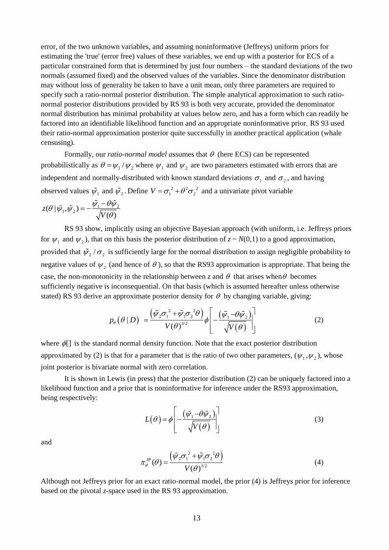
error, of the two unknown variables, and assuming noninformative (Jeffreys) uniform priors for

estimating the 'true' (error free) values of these variables, we end up with a posterior for ECS of a

particular constrained form that is determined by just four numbers – the standard deviations of the two

normals (assumed fixed) and the observed values of the variables. Since the denominator distribution

may without loss of generality be taken to have a unit mean, only three parameters are required to

specify such a ratio-normal posterior distribution. The simple analytical approximation to such ratio-

normal posterior distributions provided by RS 93 is both very accurate, provided the denominator

normal distribution has minimal probability at values below zero, and has a form which can readily be

factored into an identifiable likelihood function and an appropriate noninformative prior. RS 93 used

their ratio-normal approximation posterior quite successfully in another practical application (whale

censusing).

Formally, our ratio-normal model assumes that (here ECS) can be represented

probabilistically as 1 2/ where

1 and 2 are two parameters estimated with errors that are

independent and normally-distributed with known standard deviations 1 and 2 , and having

observed values 1 and 2 . Define 2 2 2

1 2V and a univariate pivot variable

1 21 2( | , )

( )z

V

RS 93 show, implicitly using an objective Bayesian approach (with uniform, i.e. Jeffreys priors

for 1 and 2 ), that on this basis the posterior distribution of z ~ N(0,1) to a good approximation,

provided that 2 2/ is sufficiently large for the normal distribution to assign negligible probability to

negative values of 2 (and hence of ), so that the RS93 approximation is appropriate. That being the

case, the non-monotonicity in the relationship between z and that arises when becomes

sufficiently negative is inconsequential. On that basis (which is assumed hereafter unless otherwise

stated) RS 93 derive an approximate posterior density for by changing variable, giving:

2 2

2 1 1 2 1 2

3/2

 |

( )p D

V V

(2)

where [] is the standard normal density function. Note that the exact posterior distribution

approximated by (2) is that for a parameter that is the ratio of two other parameters, ( 1 , 2 ), whose

joint posterior is bivariate normal with zero correlation.

It is shown in Lewis (in press) that the posterior distribution (2) can be uniquely factored into a

likelihood function and a prior that is noninformative for inference under the RS93 approximation,

being respectively:

1 2 

LV

(3)

and

2 2

2 1 1 2

3/2( )

( )

JP

V

(4)

Although not Jeffreys prior for an exact ratio-normal model, the prior (4) is Jeffreys prior for inference

based on the pivotal z-space used in the RS 93 approximation.

14

Frequentist analysis is also performed using the SRLR method on the likelihood function (3).

Provided the RS 93 approximation is appropriate, the RS 93 likelihood will be a transformed normal,

for which the SRLR method provides exact confidence intervals.

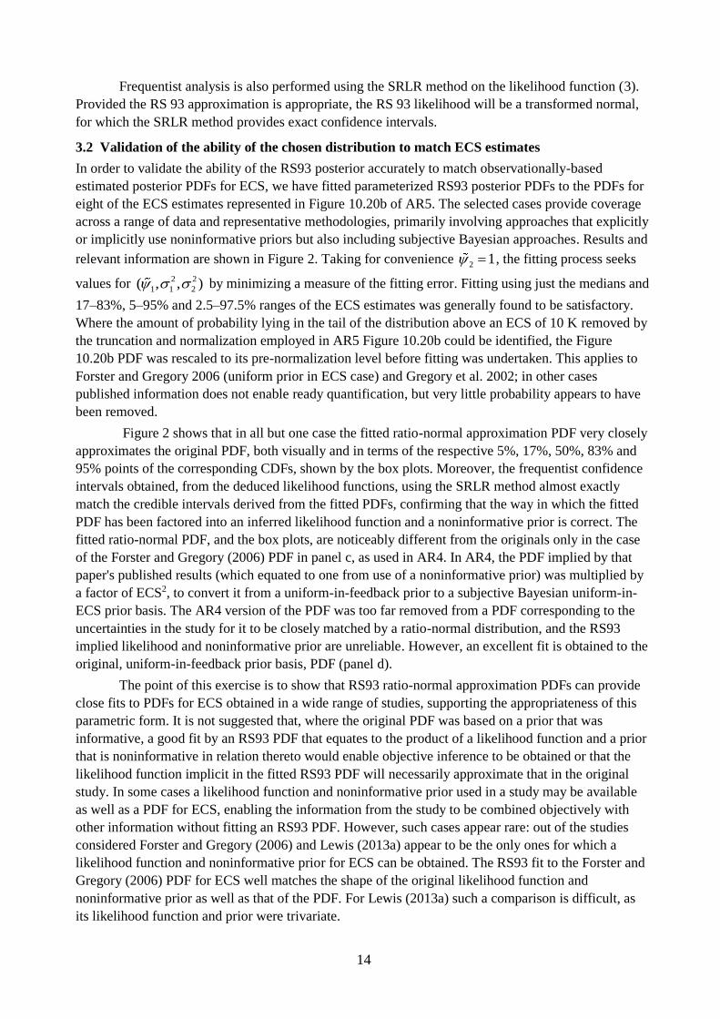
3.2 Validation of the ability of the chosen distribution to match ECS estimates

In order to validate the ability of the RS93 posterior accurately to match observationally-based

estimated posterior PDFs for ECS, we have fitted parameterized RS93 posterior PDFs to the PDFs for

eight of the ECS estimates represented in Figure 10.20b of AR5. The selected cases provide coverage

across a range of data and representative methodologies, primarily involving approaches that explicitly

or implicitly use noninformative priors but also including subjective Bayesian approaches. Results and

relevant information are shown in Figure 2. Taking for convenience 2 1 , the fitting process seeks

values for 2 2

1 1 2( , , ) by minimizing a measure of the fitting error. Fitting using just the medians and

17–83%, 5–95% and 2.5–97.5% ranges of the ECS estimates was generally found to be satisfactory.

Where the amount of probability lying in the tail of the distribution above an ECS of 10 K removed by

the truncation and normalization employed in AR5 Figure 10.20b could be identified, the Figure

10.20b PDF was rescaled to its pre-normalization level before fitting was undertaken. This applies to

Forster and Gregory 2006 (uniform prior in ECS case) and Gregory et al. 2002; in other cases

published information does not enable ready quantification, but very little probability appears to have

been removed.

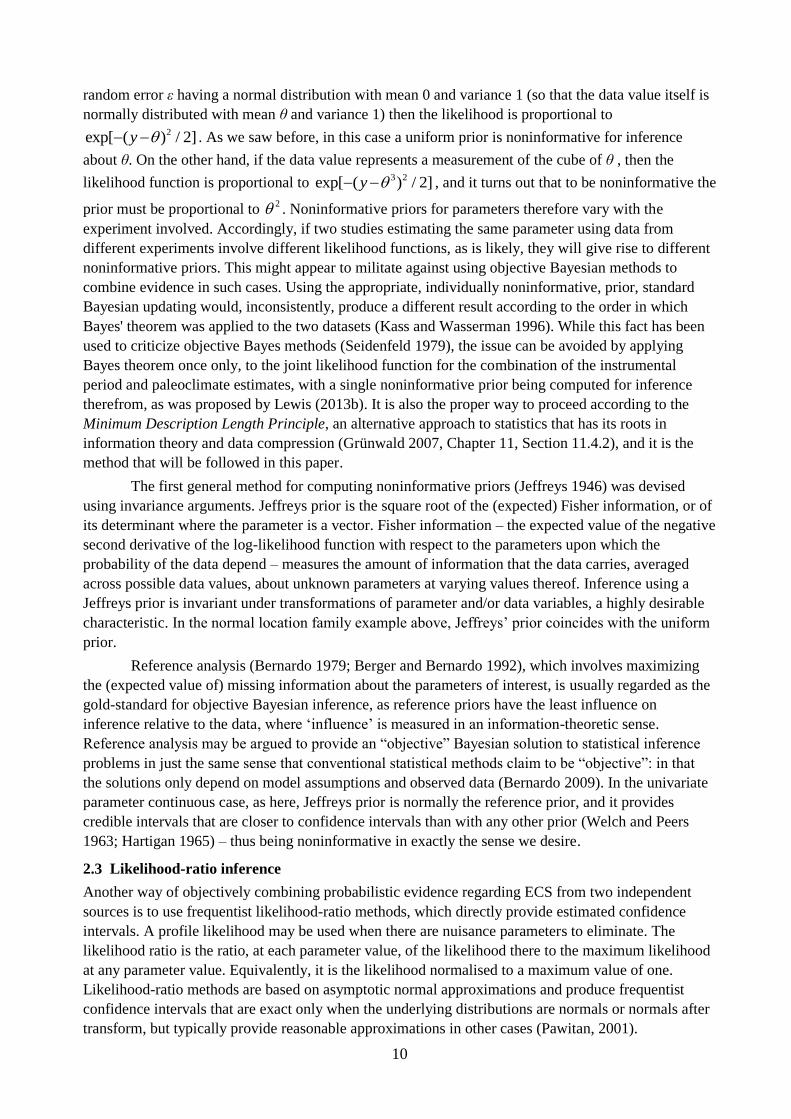
Figure 2 shows that in all but one case the fitted ratio-normal approximation PDF very closely

approximates the original PDF, both visually and in terms of the respective 5%, 17%, 50%, 83% and

95% points of the corresponding CDFs, shown by the box plots. Moreover, the frequentist confidence

intervals obtained, from the deduced likelihood functions, using the SRLR method almost exactly

match the credible intervals derived from the fitted PDFs, confirming that the way in which the fitted

PDF has been factored into an inferred likelihood function and a noninformative prior is correct. The

fitted ratio-normal PDF, and the box plots, are noticeably different from the originals only in the case

of the Forster and Gregory (2006) PDF in panel c, as used in AR4. In AR4, the PDF implied by that

paper's published results (which equated to one from use of a noninformative prior) was multiplied by

a factor of ECS2, to convert it from a uniform-in-feedback prior to a subjective Bayesian uniform-in-

ECS prior basis. The AR4 version of the PDF was too far removed from a PDF corresponding to the

uncertainties in the study for it to be closely matched by a ratio-normal distribution, and the RS93

implied likelihood and noninformative prior are unreliable. However, an excellent fit is obtained to the

original, uniform-in-feedback prior basis, PDF (panel d).

The point of this exercise is to show that RS93 ratio-normal approximation PDFs can provide

close fits to PDFs for ECS obtained in a wide range of studies, supporting the appropriateness of this

parametric form. It is not suggested that, where the original PDF was based on a prior that was

informative, a good fit by an RS93 PDF that equates to the product of a likelihood function and a prior

that is noninformative in relation thereto would enable objective inference to be obtained or that the

likelihood function implicit in the fitted RS93 PDF will necessarily approximate that in the original

study. In some cases a likelihood function and noninformative prior used in a study may be available

as well as a PDF for ECS, enabling the information from the study to be combined objectively with

other information without fitting an RS93 PDF. However, such cases appear rare: out of the studies

considered Forster and Gregory (2006) and Lewis (2013a) appear to be the only ones for which a

likelihood function and noninformative prior for ECS can be obtained. The RS93 fit to the Forster and

Gregory (2006) PDF for ECS well matches the shape of the original likelihood function and

noninformative prior as well as that of the PDF. For Lewis (2013a) such a comparison is difficult, as

its likelihood function and prior were trivariate.

15

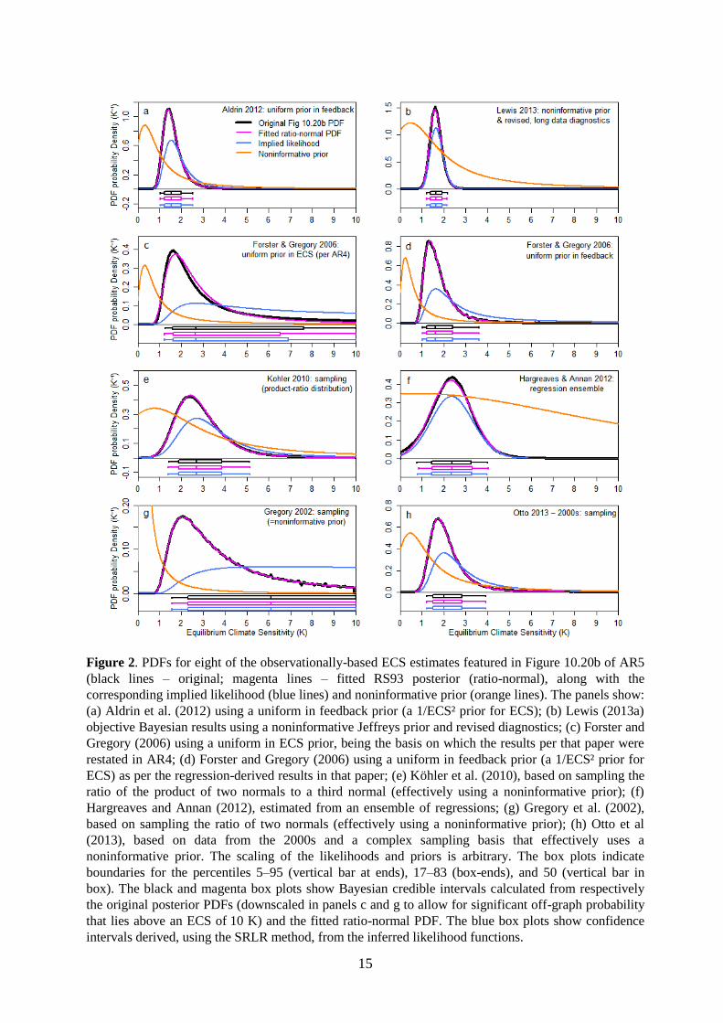
Figure 2. PDFs for eight of the observationally-based ECS estimates featured in Figure 10.20b of AR5

(black lines – original; magenta lines – fitted RS93 posterior (ratio-normal), along with the

corresponding implied likelihood (blue lines) and noninformative prior (orange lines). The panels show:

(a) Aldrin et al. (2012) using a uniform in feedback prior (a 1/ECS² prior for ECS); (b) Lewis (2013a)

objective Bayesian results using a noninformative Jeffreys prior and revised diagnostics; (c) Forster and

Gregory (2006) using a uniform in ECS prior, being the basis on which the results per that paper were

restated in AR4; (d) Forster and Gregory (2006) using a uniform in feedback prior (a 1/ECS² prior for

ECS) as per the regression-derived results in that paper; (e) Köhler et al. (2010), based on sampling the

ratio of the product of two normals to a third normal (effectively using a noninformative prior); (f)

Hargreaves and Annan (2012), estimated from an ensemble of regressions; (g) Gregory et al. (2002),

based on sampling the ratio of two normals (effectively using a noninformative prior); (h) Otto et al

(2013), based on data from the 2000s and a complex sampling basis that effectively uses a

noninformative prior. The scaling of the likelihoods and priors is arbitrary. The box plots indicate

boundaries for the percentiles 5–95 (vertical bar at ends), 17–83 (box-ends), and 50 (vertical bar in

box). The black and magenta box plots show Bayesian credible intervals calculated from respectively

the original posterior PDFs (downscaled in panels c and g to allow for significant off-graph probability

that lies above an ECS of 10 K) and the fitted ratio-normal PDF. The blue box plots show confidence

intervals derived, using the SRLR method, from the inferred likelihood functions.

16

3.3 Fitting parameterised PDFs to the instrumental and paleoclimate ECS estimates

Having demonstrated the ability of the RS93 approximation to a ratio-normal PDF accurately to

represent estimated PDFs for ECS over a range of examples, we fit it to the preferred results ECS

estimate from LC15, the primary selected representative instrumental period study, using the full LC15

PDF. The fitted PDF is not normalised to unit probability over the fitted range; since a small amount of

probability lies above that range doing so would distort the derived CDF percentile point ECS values.

The fitting process compensates for the AR5 forcing distribution being slightly skewed (which means

the denominator distribution normality assumption in RS 93 is not completely accurate) by assigning

almost all uncertainty to the denominator distribution, which increases the skewness of the fitted

distribution. Figure 3a shows the fitted PDF to be extremely close to the original. Table 1 shows that

the ECS values for the fitted distribution match those of the original within ~0.05 K at 5%, 17%, 50%,

83% and 95% CDF percentiles. Moreover, the amount of probability lying above 10 K is only

marginally smaller for the fitted PDF than the original: 1.0% vs 1.4%. Accordingly, the fit may be

regarded as very satisfactory.

For Oa13, the RS93 fit is as obtained in Section 3. That PDF is an almost perfect fit (all ECS

values match within 0.01 K up to the 95% CDF point), as shown in Figure 3a by its exact coincidence

with the original Oa13 PDF.

Whilst negative ECS values can reasonably be ruled out on the grounds that they imply cooling

in response to a positive forcing and are inconsistent with understanding of the energy balance of the

climate system, observationally-based paleoclimate ECS estimates will correctly show some

probability lying below 0 K where the fractional uncertainty in their temperature change estimate is

substantial. This is evident, for instance, with Hargreaves and Annan (2012), where their ECS estimate

PDF remains significantly positive at 0 K. It is also the case for the AR5 paleoclimate range (as 10-

90%) based estimate used here. In contrast, the AR5 instrumental period energy budget based ECS

estimates have essentially zero probability below 0 K, as the fractional uncertainty in the temperature

change involved is relatively low, even allowing for internal variability. Therefore, when the energy

budget and paleoclimate estimates are combined negligible probability lies below 0 K.

Fitting an RS93 posterior distribution to the AR5 paleoclimate evidence based 2.75 K median

estimate and 1–6 K range, treated as 10–90%, is straightforward, since with three points and three free

parameters the fit is unique. The fitted PDF has very small but non-negligible probability situated

below 0 K and above 10 K. In order to accommodate probability at negative and very high ECS values,

the fitted PDF is computed over an ECS range of −2 K to 100 K, with a 0.05% probability mass added

at −2 K to adjust for probability below that ECS level, but is not normalized to unit probability. The

fitted probability at ECS values between −2 K and 0 K arises almost entirely as a result of the

numerator normal distribution taking negative values and is therefore correctly attributable to ECS

values below zero. Figure 3a shows the fitted distribution's PDF. The three fitted CDF percentile points

are within 0.01 K of the specified values.

4. Priors and likelihoods for fitted distributions and combined evidence

4.1 Deriving a noninformative prior for inference from the combined evidence

The priors for the separate-evidence cases – LC15 and Oa13 AR5 instrumental period energy budget

based estimates, and AR5 paleoclimate evidence 1–6 K range based estimate using a 2.75 K median –

are Jeffreys priors for the fitted PDFs, derived using (4). Jeffreys prior equals the square root of Fisher

information, and the Fisher information for two independent sets of data is the sum of that for the

individual data sets. Accordingly, Jeffreys prior for inference from two independent sources of

observationally-based evidence combined is the sum in quadrature of the Jeffreys priors relating to

17

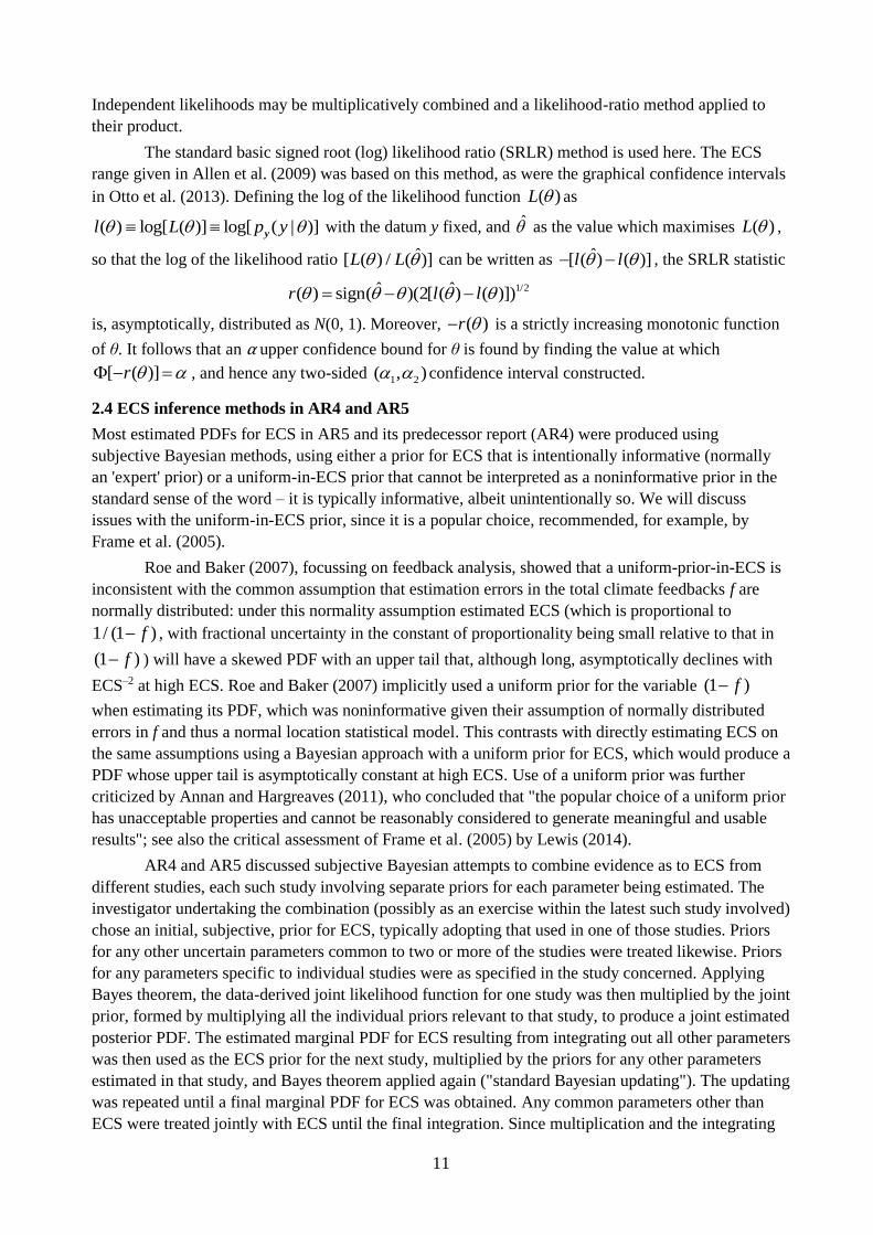
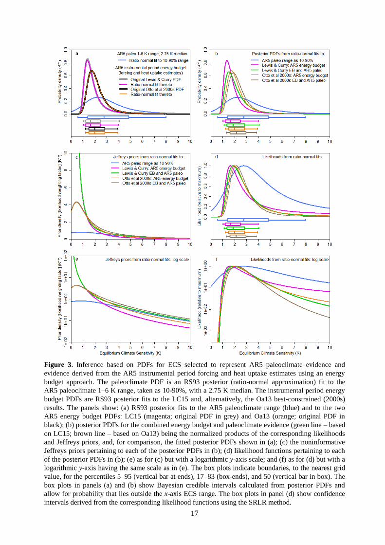
Figure 3. Inference based on PDFs for ECS selected to represent AR5 paleoclimate evidence and

evidence derived from the AR5 instrumental period forcing and heat uptake estimates using an energy

budget approach. The paleoclimate PDF is an RS93 posterior (ratio-normal approximation) fit to the

AR5 paleoclimate 1–6 K range, taken as 10-90%, with a 2.75 K median. The instrumental period energy

budget PDFs are RS93 posterior fits to the LC15 and, alternatively, the Oa13 best-constrained (2000s)

results. The panels show: (a) RS93 posterior fits to the AR5 paleoclimate range (blue) and to the two

AR5 energy budget PDFs: LC15 (magenta; original PDF in grey) and Oa13 (orange; original PDF in

black); (b) posterior PDFs for the combined energy budget and paleoclimate evidence (green line – based

on LC15; brown line – based on Oa13) being the normalized products of the corresponding likelihoods

and Jeffreys priors, and, for comparison, the fitted posterior PDFs shown in (a); (c) the noninformative

Jeffreys priors pertaining to each of the posterior PDFs in (b); (d) likelihood functions pertaining to each

of the posterior PDFs in (b); (e) as for (c) but with a logarithmic y-axis scale; and (f) as for (d) but with a

logarithmic y-axis having the same scale as in (e). The box plots indicate boundaries, to the nearest grid

value, for the percentiles 5–95 (vertical bar at ends), 17–83 (box-ends), and 50 (vertical bar in box). The

box plots in panels (a) and (b) show Bayesian credible intervals calculated from posterior PDFs and

allow for probability that lies outside the x-axis ECS range. The box plots in panel (d) show confidence

intervals derived from the corresponding likelihood functions using the SRLR method.

18

each of them separately. Denoting those evidence sources A and B, where the RS93 ratio-normal

approximation is used the combined-inference prior is thus:

AB

2 22 2 2 2

A2 A1 A1 A2 B2 B1 B1 B2

3 32 2 2 2 2 2

A1 A2 B1 B2

( )

JP

(5)

It was shown in Lewis (in press) that combining on this basis priors of the form in (4) relating to two

independent sources of evidence, A and B, each represented by a RS93 posterior PDF, produces

inference with excellent probability matching properties. That is, when tested by repeated sampling

from the two pairs of normal distributions involved, Bayesian credible intervals derived from using

such a prior with the two likelihood functions of the form in (3) multiplicatively-combined, prove to be

almost exact confidence intervals. Lewis (in press) also shows that the (standard, but generally

incorrect) method of Bayesian updating, simply using a noninformative prior for one of the two

likelihoods, has substantially worse probability matching properties compared to the method described

above; see Section 6 for more discussion.

4.2 Characteristics of the different priors

Figure 3c shows the prior relating to each of the three separate-evidence fitted RS93 posterior PDFs

and for the two combined-evidence cases. The Jeffreys priors for the instrumental period and

paleoclimate RS93 posterior fits have different shapes, more easily seen when plotted on a log scale

(Figure 3e). At very high ECS values, in all cases the prior declines as ECS–2. Very high ECS values

are far more likely to arise from the denominator normal being very small – close to zero – than from

the numerator normal being extremely large. Small changes in the denominator normal as it

approaches zero translate into very large changes in ECS, so the data is increasingly uninformative

about ECS, even if the likelihood is still significant. Accordingly, the Jeffreys prior declines as ECS

increases, down-weighting the likelihood. Put another way, because of their reciprocal relationship, a

small region of the denominator normal CDF near zero (representing near zero ΔFn or n( )F Q

values) maps into a large range of high values for ECS. That requires the prior to decline with ECS−2

(the same as the Jacobian factor used to convert PDFs when a variable is changed to its reciprocal) in

order to preserve matching of probability between data space and parameter space. As explained in

section 3.3, the optimized ratio-normal approximation fit to the LC15 instrumental period ECS

estimate gives almost zero standard deviation to the numerator normal distribution (which represents

ΔT). As a result, in this case at low ECS levels the prior continues to rise nearly with ECS−2 as ECS

declines, before peaking when ECS is just above zero. Since the likelihood function declines much

more rapidly as ECS approaches zero than the prior increases, the fitted posterior PDF nevertheless

tracks the sharply declining original.

The Jeffreys prior for the paleoclimate-evidence based fitted PDF declines much more gently

with ECS at moderate ECS values than do the instrumental period fitted PDFs, reflecting the relatively

greater informativeness of paleoclimate evidence over this range.

At low ECS levels, the priors for inference from the combined instrumental period and

paleoclimate evidence are dominated by the high Jeffreys priors from the instrumental period evidence,

but as ECS rises and those priors declines rapidly – reflecting increments in ECS corresponding to

increasingly smaller areas in data-space – the combined-evidence priors deviate towards the

paleoclimate prior, in each case asymptoting to a modest multiple of it at high ECS values.

4.3 Likelihoods

Figure 3d shows (normalized to unit maximum) the likelihood functions given by (3) that correspond,

using the relevant Jeffreys prior, to the fitted RS93 posterior distributions for the LC15 and Oa13

instrumental period energy budget estimates and for the RS93 posterior distribution that matches the

19

PDF concerned

and relevant

characteristic

RS93 numerator

normal distribution

RS93 denominator

normal distribution

ECS at

5%

CDF or

CI point

(K)

ECS at

17%

CDF or

CI point

(K)

ECS at

50%

CDF or

CI point

(K)

ECS at

83%

CDF or

CI point

(K)

ECS at

95%

CDF or

CI point

(K)

Mean Standard

deviation

Mean Standard

deviation

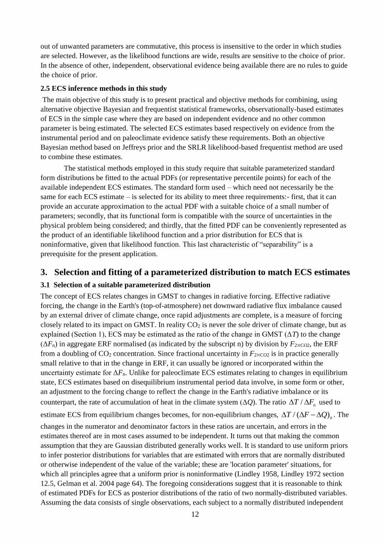
Original LC15 - - - - 1.05 1.25 1.64 2.45 4.05

Instrumental period:

fitted to LC15 PDF 1.635 0.000 1 (fixed) 0.359

1.05

1.05

1.2

1.2

1.64

1.64

2.5

2.5

4.0

4.0

Fitted LC15 adjusted

for time-varying EffCS 1.787 0.193 1 (fixed 0.359

1.1

1.1

1.3

1.3

1.79

1.79

2.75

2.75

4.40

4.40

Instrumental period:

fitted to Oa13 PDF 1.991 0.321 1 (fixed) 0.288

1.2

1.2

1.5

1.5

1.99

1.99

2.85

2.85

3.9

3.9

Paleo: fitted to range

as 10-90% & median 2.750 1.317 1 (fixed) 0.361

0.55

0.55

1.4

1.4

2.75

2.75

4.85

4.85

7.95

7.95

Combined fitted LC15

+ paleo 10-90% - - - -

1.1

1.1

1.35

1.35

1.88

1.86

2.85

2.85

4.05

4.05

Combined fitted LC15

adjusted for varying

EffCS +paleo 10-90%

- - - - 1.2

1.2

1.45

1.45

2.02

2.01

3.0

3.0

4.2

4.2

Combined fitted Oa13

+ paleo 10-90% - - - -

1.3

1.3

1.6

1.6

2.14

2.13

2.95

2.95

3.85

3.85

Bayesian update PDFs

LC15 PDF fit updated

by paleo fit likelihood 1.1 1.3 1.77 2.6 3.6

Paleo PDF fit updated

by LC15 fit likelihood 1.25 1.55 2.20 3.3 4.65

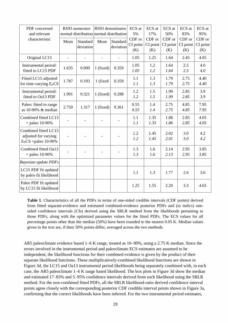
Table 1. Characteristics of all the PDFs in terms of one-sided credible intervals (CDF points) derived

from fitted separate-evidence and estimated combined-evidence posterior PDFs and (in italics) one-

sided confidence intervals (CIs) derived using the SRLR method from the likelihoods pertaining to

those PDFs, along with the optimized parameter values for the fitted PDFs. The ECS values for all

percentage points other than the median (50%) have been rounded to the nearest 0.05 K. Median values

given in the text are, if their 50% points differ, averaged across the two methods.

AR5 paleoclimate evidence based 1–6 K range, treated as 10–90%, using a 2.75 K median. Since the

errors involved in the instrumental period and paleoclimate ECS estimates are assumed to be

independent, the likelihood functions for their combined evidence is given by the product of their

separate likelihood functions. These multiplicatively-combined likelihood functions are shown in

Figure 3d, the LC15 and Oa13 instrumental period likelihoods being separately combined with, in each

case, the AR5 paleoclimate 1–6 K range based likelihood. The box plots in Figure 3d show the median

and estimated 17–83% and 5–95% confidence intervals derived from each likelihood using the SRLR

method. For the non-combined fitted PDFs, all the SRLR likelihood-ratio derived confidence interval

points agree closely with the corresponding posterior CDF credible interval points shown in Figure 3a,

confirming that the correct likelihoods have been inferred. For the two instrumental period estimates,

20

where there is no probability at below 0 K to degrade the RS93 fit, the match is effectively exact: at all

percentage points the credible interval and confidence interval ECS values are identical to three

decimal places. For the AR5 paleoclimate range based distribution, the match is within 0.02 K up to

the 95% point (7.95 K).

Figure 3f shows the likelihoods plotted on the same log scale as for the priors in Figure 3e.

Since Bayes theorem, (1), involves addition rather than multiplication when the terms are replaced by

their logarithms, the relative influences of the prior and likelihood on each of the posterior PDFs may

be appraised by comparing the lines of the relevant color in Figure 3e and 3f.

5. Results

Figure 3b shows the posterior PDFs for the combined instrumental period and paleoclimate evidence

cases, derived from the product of the corresponding Jeffreys priors and likelihoods. These PDFs have

been normalized to unit probability over the fitted range, which captures essentially all probability.

They produce a 5–95% range for climate sensitivity of 1.1–4.05 K, median 1.87 K, based on the

primary, LC15, fitted distribution. Using the alternative Oa13 fitted distribution gives a 5–95% range

of 1.3–3.85 K, with a median of 2.14 K.

Figure 3b also replicates, for comparison, the fitted posterior PDFs shown in Figure 3a for the

separate ECS estimates derived from the LC15 and Oa13 AR5 instrumental period energy budget and

the AR5 paleoclimate evidence based estimates. These PDFs equate to the normalised product of the

corresponding Jeffreys priors and likelihoods shown in Figures 3c and 3d.

The combined-evidence PDFs are largely dominated by the region of overlap of the two input

datasets, and may be viewed as either an update of the paleoclimate evidence using instrumental period

energy budget data or vice versa. Viewed from the first perspective, the instrumental data greatly

sharpens the paleoclimate data, raising the 5% point but bringing down the median, 83% and 95%

points. Viewed from the second perspective, the paleoclimate evidence increases the median and 83%

point of the instrumental evidence – more so for LC15 than Oa13 – reflecting the paleoclimate

estimate having a much higher median and upper tail. That uncertainty can increase despite additional

knowledge is well-established (Hannart et al. 2013). The left hand tail of the combined-evidence PDFs

is largely controlled by the extremely sharp cutoff below 1 K observable in both energy-budget study

fitted (and actual) PDFs. The combined-evidence 95% point is a little higher than for the instrumental

period energy-budget estimate alone for LC15, but a little lower for Oa13, in both cases representing a

substantial reduction from the estimate based on the paleoclimate data alone. For both LC15 and Oa13,

the upper tails of the combined evidence distributions beyond the 95% point decline much faster than

that for the instrumental period energy budget estimate alone.

It is also relevant to compare, for the combined-evidence cases, the confidence interval

percentage points from using the SRLR method on their multiplicatively-combined likelihood

functions with the credible interval percentage points derived from the Bayesian posterior PDFs. The

box plots in Figure 3b and 3d shows the ECS values at 5%, 17%, 50%, 83% and 95% points for the

respective methods. It can be seen that agreement between results from the two fundamentally different

statistical approaches is very close at all five percentile points. Table 1 gives the ECS values at the 5%,

17%, 50%, 83% and 95% CDF points (tops of one-sided credible intervals) for all the PDFs, and for

the corresponding one-sided confidence intervals derived using the SRLR method for all the fitted and

combined likelihoods, along with the optimized parameter values for the fitted PDFs.

The forcing and heat uptake estimates given in AR5, used in LC15, ended in 2011. Strong

warming has occurred since then, and ocean heat uptake has increased. We have updated the LC15

main results by extending the final period to 1995–2015, using primarily observational data for post-

2011 changes in forcing and heat uptake and version 4 of the HadCRUT4 GMST dataset

21

(supplementary material: S1). Although the updated transient climate response estimate (median 1.34

K, 5–95% range 0.9–2.45 K) is virtually unchanged, the updated ECS estimate has a slightly higher

median of 1.75 K, reflecting greater estimated ocean heat uptake, and is worse constrained above (5–

95% range 1.1–4.5 K). Using this updated ECS estimate, the median of the resulting combined-

evidence posterior distribution is 0.1 K higher than when based on the non-updated LC15 fitted PDF,

whilst the 95% point is 0.15 K higher. The latter increase is much less than the 0.4 K increase in the

LC15 fitted PDF 95% point caused by the updating, reflecting the fact that the paleoclimate evidence

contributes more to constraining the upper tail of the combined ECS estimate when the upper tail of the

instrumental evidence is less well constrained.

Paleoclimate ECS estimates, except where based on changes during the Holocene, normally

reflect differences in equilibrium climate states. Energy budget ECS estimates, however, reflect

climate feedback strength over the instrumental period, and thus strictly are of effective climate

sensitivity (EffCS) rather than ECS. In many AOGCMs, EffCS is time-varying and starts off lower than

ECS. To investigate sensitivity of the combined-evidence ECS estimates to the possibility that ECS

similarly exceeds EffCS in the real world, the LC15 fitted distribution is divided by a N(0.925,0.10)

distribution and a revised RS93 distribution fitted. A N(0.925,0.10) distribution is considered to be

representative of the relationship in current generation AOGCMs between EffCS derivable from the

instrumental-period forcing profile and ECS as usually diagnosed (supplementary material: S2). The

median and 95% point of the resulting combined-evidence posterior distribution are both 0.15 K higher

than when based on the unadjusted LC15 fitted PDF.

The supplementary material includes (S3) a comparison of the results obtained here with those

obtained using a shifted log-t distribution as the functional form to fit the PDFs, instead of the RS93

posterior based on the ratio-normal model. This is done (a) to underline the important point that the

concepts demonstrated in this paper are not restricted to the use of a single functional form, (b) to

demonstrate the superiority of the RS93 ratio-normal approximation in this particular instance and (c)

to provide a direct comparison of the final results against a distribution that has been used to represent

ECS estimates and other skewed PDFs by previous authors.

6. Discussion

We have combined independent evidence about ECS with different uncertainty characteristics, each

representable by a ratio-normal distribution, using an objective Bayesian method that has been shown

elsewhere to provide accurate probability matching when combining such evidence. Previous studies

have used subjective Bayesian approaches, which almost certainly involved priors that led to results

different from those implied by the observational data used. If, for this present study, inference from

the combined evidence had been performed using a uniform rather than noninformative prior for ECS,

but with the same likelihood functions derived from the fitted ratio-normal approximation RS93

posteriors, the 95% uncertainty bound (CDF point) for ECS from the combined evidence would have

been far higher, at 13.45 K. The median estimate would also have been substantially higher, at 2.58 K.

This offers a clear example of a subjective informative prior greatly distorting inference.

Using standard Bayesian updating to combine instrumental and paleoclimate evidence

produces results that vary according to ordering (Table 1, bottom section) and disagree with those

obtained using the objective Bayesian method. Updating the LC15 fitted RS93 posterior by

multiplying it by the likelihood function inherent in the RS93 fit to the paleoclimate evidence gives a

median ECS estimate of 1.77 K and 95% bound of 3.6 K. Reversing the ordering, taking the PDF from

the paleoclimate evidence and updating it with the likelihood pertaining to the LC15 fitted distribution,

increases the median to 2.20 K and the 95% bound to 4.65 K. In neither case is inference close to that

from the objective method (1.88 K median, 4.05 K 95% bound).

22

The probability matching of posterior PDFs derived by combining observationally-based

evidence involving two different likelihood functions using a prior that is the sum in quadrature of the

separate-evidence Jeffreys priors, has also been tested and found to be accurate in cases involving very

different probability distributions from those considered here (Lewis 2013a, Supplemental

Information; Lewis 2013b).

Both the objective Bayesian and likelihood-ratio methods used here require likelihood

functions pertaining to each source of evidence. It is therefore highly desirable for probabilistic results

presented by scientific studies to include full (joint) likelihood functions, as well as joint posterior

PDFs. In this case, despite likelihood functions being unavailable, it proved possible to estimate them

by fitting ratio-normal approximation distributions to the posterior PDFs or percentile points available,

but often such a route would not be available.

The approach used here requires that the uncertainties involved in the two sources of evidence

are independent. Combining different evidence for ECS from the instrumental period is more

challenging because, given the influence of climate system internal variability, errors in different lines

of evidence are unlikely to be fully independent. Some instrumental period studies that use multiple

data variables (Forest et al. 2006, Lewis 2013a) have explicitly sought to address independence issues,

using optimal fingerprint techniques based on covariances estimated from unforced control runs of

AOGCMs to transform data variables into an approximately conditionally-independent set of variables,

despite imperfect representation of internal variability. In suitable cases information derived from such

AOGCM control runs might likewise enable correlated variables from different studies to be so

transformed, and thus widen the scope for combining evidence regarding ECS. However, even if

successful, the observed changes over the instrumental period only represent a single realisation of

internal climate variability, and some principal uncertainties likely affect all aspects of the resulting

ECS estimate.

Where other uncertain parameters have been estimated alongside ECS by different sets of data,

it is necessary to combine evidence for all common parameters jointly and only seek a marginal

distribution for ECS at the final stage. That is potentially relevant where combining instrumental and

non-equilibrium recent paleoclimate evidence (Hegerl et al. 2006), adding complexity, but when the

paleoclimate period concerned is more distant and changes are quasi-equilibrium ECS is typically the

only common constrained parameter.

Acknowledgements

We thank Marcel Crok and Tore Schweder for bringing us together; Paul Kirwan, Tore

Schweder and an anonymous reviewer for helpful comments that improved the manuscript and Oliver

Browne for supplying PDF data underlying AR5 Figure 10.20b. Peter Grünwald was supported by an

NWO VICI Grant. NWO is the Netherlands foundation for scientific research.

References

Aldrin, M., et al., 2012: Bayesian estimation of climate sensitivity based on a simple climate model fitted to

observations of hemispheric temperatures and global ocean heat content. Environmetrics, 23, 253-271.

Allen M. R., D. J. Frame, C. Huntingford, C. D. Jones, J. A. Lowe, M. Meinshausen and N. Meinshausen,

2009: Warming caused by cumulative carbon emissions towards the trillionth tonne. Nature, 458,

1163-6.

Andronova, N.G. and M.E Schlesinger, 2001: Objective estimation of the probability density function for

climate sensitivity. J. Geophys. Res., 106, D19, 22, 605–22,611.

Annan, J. D., J. C. Hargreaves, R. Ohgaito, A. Abe-Ouchi, and S. Emori, 2005: Efficiently constraining

climate sensitivity with ensembles of paleoclimate simulations. Sci. Online Lett. Atmos., 1, 181–184

23

Annan, J. D., and J. C. Hargreaves, 2006: Using multiple observationally-based constraints to estimate

climate sensitivity. Geophys. Res. Lett., 33, L06704.

Annan, J. D., and J. C. Hargreaves, 2011: On the generation and interpretation of probabilistic estimates of

climate sensitivity. Climatic Change, 104,3-4, 423-436.

Annan, J. D. and J. C. Hargreaves, 2013. A new global reconstruction of temperature changes at the Last

Glacial Maximum. Clim. Past, 9, 367–376.

Bayes, T, 1763: An essay towards solving a problem in the doctrine of chances. Philos. Trans. R. Soc.

Lond. 53 (1763) 370–418; 54 (1764) 269–325. Reprinted in Biometrika 45 (1958), 293-315.

Berger J O and J. M. Bernardo, 1992: On the development of reference priors (with discussion). In:

Bernardo J. M., Berger J. O., Dawid A. P., Smith A. F. M. (eds) Bayesian Statistics 4. Oxford

University Press, pp 35-60.

Berger, J. (2006): The case for objective Bayesian analysis. Bayesian analysis, 1(3), 385-402.

Bernardo J. M., 1979: Reference posterior distributions for Bayesian inference (with discussion). J Roy

Statist Soc Ser B, 41,113–147.

Bernardo, J.M., 2009. Modern Bayesian Inference: Foundations and Objective Methods, 263–306. In

Philosophy of Statistics, P. Bandyopadhyay and M. Forster, eds. North Holland, Oxford, UK, 1253 pp.

Chylek, P. and U. Lohmann, 2008: Aerosol radiative forcing and climate sensitivity deduced from the last

glacial maximum to Holocene transition. Geophys. Res. Lett., 35, L04804.

Colman, R. and B. McAvaney, 2009. Climate feedbacks under a very broad range of forcing. Geophys.

Res.Lett., 36, L01702,doi:10.1029/2008GL036268

Forest, C.E., P. H. Stone and A. P. Sokolov, 2006: Estimated PDFs of climate system properties including

natural and anthropogenic forcings. Geophys. Res. Lett., 33, L01705, doi:10.1029/2005GL023977.

Forster P. M. de F. and J. M. Gregory, 2006: The Climate Sensitivity and Its Components Diagnosed from

Earth Radiation budget data. J. Climate, 19, 39–52.

Frame, D. J., B. B. B. Booth, J. A. Kettleborough, D. A. Stainforth, J. M. Gregory, M. Collins, and M. R.

Allen, 2005: Constraining climate forecasts: The role of prior assumptions. Geophys. Res. Lett., 32,

L09702, doi:10.1029/2004GL022241

Fraser, D. A. S., N. Reid, E. Marras and G. Y. Yi, 2010: Default priors for Bayesian and frequentist

inference. J. R. Statist. Soc. B, 72, 5, 631-654.

Friedrich, T., et al., 2016. "Nonlinear climate sensitivity and its implications for future greenhouse

warming." Science Advances 2, 11, e1501923.

Gelman, A., Carlin, J.B., Stern, H.S. and Rubin, D.B., 2004. Bayesian data analysis. Chapman and

Hall/CRC, Boca Raton, Florida, 690

Gregory J., R. J.Stouffer, S. C. B. Raper, P. A. Stott, and N. A. Rayner, 2002: An Observationally Based

Estimate of the Climate Sensitivity. J. Climate, 15, 3117–3121.

Grünwald, 2007: The Minimum Description Length Principle. MIT Press, Cambridge, Massachusetts.

Hannart A., M. Ghil, J-L. Dufresne and P. Naveau, 2013: Disconcerting learning on climate sensitivity and

the uncertain future of uncertainty. Climatic Change, 119, 585-601.

Hargreaves, J. C., A. Abe-Ouchi. and J. D. Annan, 2007. Linking glacial and future climates through an

ensemble of GCM simulations. Clim. Past, 3, 77–87.

Hargreaves, J. C., J. D. Annan, M. Yoshimori, and A. Abe-Ouchi, 2012: Can the Last Glacial Maximum

constrain climate sensitivity? Geophys. Res. Lett., 39, L24702.

Hartigan, J.A., 1965: The Asymptotically Unbiased Prior Distribution, Ann. Math. Statist., 36, 4, 1137-

1152.

Hegerl G., T. C. Crowley, W. T. Hyde and D. J. Frame, 2006: Climate sensitivity constrained by

temperature reconstructions over the past seven centuries. Nature, 440, 1029–1032,

doi:10.1038/nature04679.

Holden, P. B., N. R. Edwards, K. I. C. Oliver, T. M. Lenton, and R. D. Wilkinson, 2010: A probabilistic

calibration of climate sensitivity and terrestrial carbon change in GENIE-1. Clim. Dyn., 35, 785–806.

Jeffreys, H., 1946: An Invariant Form for the Prior Probability in Estimation Problems. Proc. Roy. Soc. A,

186, 453–461.

24

Kass, R. E. and L. Wasserman, 1996: The Selection of Prior Distributions by Formal Rules. J. Amer. Stat.

Ass., 91, 435, 1343-1370.

Köhler, P., R. Bintanja, H. Fischer, F. Joos, R. Knutti, G. Lohmann, and V. Masson- Delmotte, 2010: What

caused Earth’s temperature variations during the last 800,000 years? Data-based evidence on radiative

forcing and constraints on climate sensitivity. Quat. Sci. Rev., 29, 129–145.

Lewis, N., 2013a: An objective Bayesian improved approach for applying optimal fingerprint techniques to

estimate climate sensitivity. Journal of Climate, 26, 7414-7429.

Lewis, N., 2013b: Modification of Bayesian Updating where Continuous Parameters have Differing

Relationships with New and Existing Data. arXiv:1308.2791 [stat.ME].

Lewis, N., 2014: Objective Inference for Climate Parameters: Bayesian, Transformation of Variables and

Profile Likelihood Approaches. J Climate, 27, 7270-7284.

Lewis, N., in press: Combining independent Bayesian posteriors into a confidence distribution, with

application to estimating climate sensitivity. Journal of Statistical Planning and Inference.

Lewis, N., J. A. Curry, 2015: The implications for climate sensitivity of AR5 forcing and heat uptake

estimates. Clim. Dyn., 45, 1009–1023.

Lindley, D. V., 1958. Fiducial Distributions and Bayes Theorem. J. Roy. Statist, Soc. B, 20, 1, 102-107

Lindley, D.V., 1972. Bayesian statistics: A review. Philadelphia: Society for industrial and applied

mathematics.

Martinez-Boti MA, G.L. Foster, T.B. Chalk, E. J. Rohling, P.F. Sexton, D.J. Lunt, R.D. Pancost, M.P.S.

Badger, D.N. Schmidt, 2015. Plio-Pleistocene climate sensitivity evaluated using high-resolution CO2

records. Nature, 518, 49–54.

Morice C. P., Kennedy J.J., Rayner N.A., Jones P.D., 2012: Quantifying uncertainties in global and regional

temperature change using an ensemble of observational estimates: The HadCRUT4 data set. J Geophys

Res, 117: D08101 doi:101029/2011JD017187.

Otto A, Otto FEL, Boucher O, Church J, Hegerl G, Forster PM, Gillett NP, Gregory J, Johnson GC, Knutti

R, Lewis N, Lohmann U, Marotzke J, Myhre G, Shindell D, Stevens B, Allen MR., 2013: Energy

budget constraints on climate response. Nature Geosci, 6, 415–416.

Otto-Bliesner, B. L., et al., 2009: A comparison of PMIP2 model simulations and the MARGO proxy

reconstruction for tropical sea surface temperatures at last glacial maximum. Clim. Dyn., 32, 799–815.

Palaeosens Project Members, 2012: Making sense of palaeoclimate sensitivity. Nature, 491, 683–691.

Pawitan, Y., 2001: In all Likelihood: Statistical Modeling and Inference Using Likelihood Ch. 3.4. Oxford

Univ. Press, 514 pp.

Raftery, A.E. and Schweder, T., 1993: Inference About the Ratio of Two Parameters, With Application to

Whale Censusing. The American Statistician, 47, 4, 259-264.

Roe, G. H., and M. B. Baker, 2007: Why is climate sensitivity so unpredictable? Science 318, 5850, 629-

632.

Schmittner, A., et al., 2012: Climate sensitivity estimated from temperature reconstructions of the last

glacial maximum. Science, 334 (2011), 1385–1388; and Response to comment on “Climate sensitivity

estimated from temperature reconstructions of the Last Glacial Maximum”. Science, 337 (2012), 1294

Schneider von Deimling, T., H. Held, A. Ganopolski, and S. Rahmstorf, 2006: Climate sensitivity estimated

from ensemble simulations of glacial climate. Clim. Dyn., 27, 149–163.

Seidenfeld, T., 1979. Why I am not an objective Bayesian; Some reflections prompted by Rosenkrantz.

Theory and Decision, 11.4, 413-440.

Snyder, C. W., 2016. Evolution of global temperature over the past two million years. Nature, 538, 226–

228

Stevens, B., S. C. Sherwood, S. Bony and M. J.Webb, 2016. Prospects for narrowing bounds on Earth's

equilibrium climate sensitivity. Earth's Future, 4, 512–522.

Szabó, B., A. van der Vaart and H. van Zanten, 2015. Frequentist coverage of adaptive nonparametric

Bayesian credible sets. Ann. Statist., 43(4), 1391-1428.

Welch, B.L. and H. W. Peers, 1963: On formulae for confidence points based on integrals of weighted

likelihoods. J. Roy. Soc. Ser. B, 25, 318-329