Numeriska beräkningar i Naturvetenskap och Teknik 1. Numerical differentiation and quadrature Discrete differentiation and integration Trapezoidal and

Numeriska beräkningar i Naturvetenskap och Teknik

1. Numerical differentiation and quadrature

Discrete differentiation and integration

Trapezoidal and Simpson’s rules

2. Ordinary differential equations

Euler’s method, Runge-Kutta methods

3. Systems of differential equations

4. Initial value and boundary problem

Shooting method

Numerical differentiation och quadratur


0f1f 1f

0x hx 0hx 0x

)(xfFunction f(x) in three points:x0-h, x0, x0+h

b

a

dxxfxf )(),('


Derivative

)('''!3

''!2

')( 432

0 xOfx

fx

xffxf

)('''!3

''!2

')( 432

001 hOfh

fh

hffhxff

f in the points: x0±h

Taylor expansion around x0=0 gives Maclaurin:


Derivative with Taylor expansion

Difference

}0{)()( 00011 xhxfhxfff

)(''!2

')(''!2

' 32

03

2

0 hOfh

hffhOfh

hff

)('2 3hOhf

)(2

' 211 hOh

fff

Derivative in three point form Local error


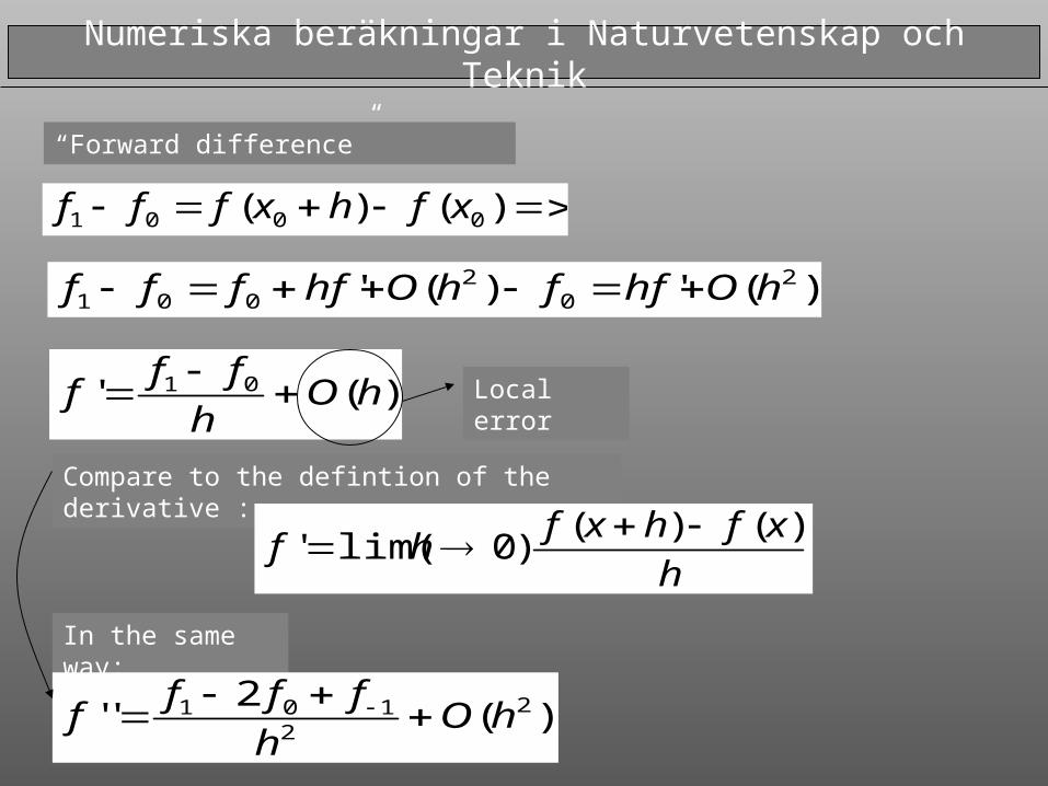
“Forward difference”

)()( 0001 xfhxfff

)(')(' 20

2001 hOhffhOhffff

)(' 01 hOh

fff

Compare to the defintion of the derivative :

h

xfhxfhf

)()()0lim('

Local error

In the same way:

)(2

'' 22

101 hOh

ffff


Quadrature: Trapetzoidal rule

0f

1f1f

0x hx hx 0x

)(xfLinear interpolation


Trapetzoidal rule

...)()()(4

2

2

ha

ha

b

a

ha

a

dxxfdxxfdxxf

(?)2

)2(

2

)(2

)(2

2

)(2

2

)(

2

)(2)(

101110

1100

10010

01102

0

Offfhffh

hf

ffhhfhf

ffffhhf

ffhffhhfAdxxf

ha

a

Area between x-h and x+h

h h

f-1

f1

f0

)(2

2)(

2

24

)(2

)()(

)(2

)()(

310131100

3

0

010

30

100

hOhfff

hOhffff

hOhff

hfdxxf

hOhff

hfdxxf

h

h

h

b

h

a


Trapetzoidal rule with error estimate:

€

[−h,0] : fa (x) = f0 +( f0 − f−1)

hx +O(x 2)

)()(

)(:],0[ 2010 xOx

h

fffxfh b

f-1

f0

f1

h

h


)(''!2

')( 32

0 xOfx

xffxf

)(!3

''22)( 5

3

0 hOhf

hfdxxfh

h

f-1

f0

f1

h

h

Simpson’s rule: Approximate by Taylor expansion

Integrated over x gives 0

)(2

'' 22

101 hOh

ffff

)()4(3

)(3

22

)()(3

22)(

5101

51010

522

10130

hOfffh

hOfff

hhf

hOhOh

fffhhfdxxf

h

h


Ordinary differential equations

An ordinary differential equation is defined as:

),...,',,( )1()( nn yyyxfy

),(' yxfy )',,('' yyxfy

First order Second order

),,(2

2

dt

rdrtF

dt

rdm

xyy '

kNdt

dN

kxdt

xdm

2

2


Euler’s method, discrete solution of first order ordinary diff. equations

)(' 1 hOh

yyy nn

Based on the “forward difference” given above:

),(' yxfy

)(),( 21 hOyxhfyy nnnn

which gives:


Runge-Kutta methods

Start by integrating between step n and n+1

1

),(),( 1

n

n

x

x

nn dxyxfyyyxfdx

dy

Taylor series for f(x,y) around the central point n+1/2

)(')(

)(),(')(),(),(2

2/12/12/1

22/12/12/12/12/1

xOfxxf

xOyxfxxyxfyxf

nnn

nnnnn

Integrate:

1

1

|)('2

)(

)(')(

32/1

22/1

2/1

22/12/12/11

n

n

n

n

xxn

nnn

x

x

nnnnn

xOfxx

xfy

dxxOfxxfyy


i.e.

)(

))(('2

)()(

'2

)()(

|)('2

)()(

32/1

32/12/1

22/1

2/12/1

2/1

22/11

2/12/11

32/1

22/1

2/12/11

hOhfy

xxOfxx

fxx

fxx

fxxy

xOfxx

fxxy

nn

nnnnn

nnn

nnn

nnnn

xxn

nnnn

n

n

)( 32/11 hOhfyy nnn


Now one needs an estimate of fn+1/2 in the expression:

)( 32/11 hOhfyy nnn

Use Euler!

)(),( 21 hOyxhfyy nnnn

At half way between points:

),(22/1 nnnn yxfh

yy

i.e. with:

)()2

,2

()( 332/11 hO

ky

hxhfyhOhfyy nnnnnn

),( nn yxhfk

Runge-Kutta of order 2 is given by:


)()2

,2

()( 332/11 hO

ky

hxhfyhOhfyy nnnnnn

Runge-Kutta of order 2

yn+1 to order h3 at the cost of calculating f(x,y) in two points.

Geometrical picture:

x

ny

1ny2/1ny

nx 1nx2/1nx

2

h

2

h

y


Runge-Kutta error of order 4 > rk3

),(1 nn yxhfk

)2

,2

(2

ky

hxhfk nn

)2,( 213 kkyhxhfk nn

)()4(6

1 43211 hOkkkyy nn


Runge-Kutta error of order 5 > rk4

),(1 nn yxhfk

)2

,2

( 12

ky

hxhfk nn

),( 34 kyhxhfk nn

)()22(6

1 543211 hOkkkkyy nn

)2

,2

( 23

ky

hxhfk nn


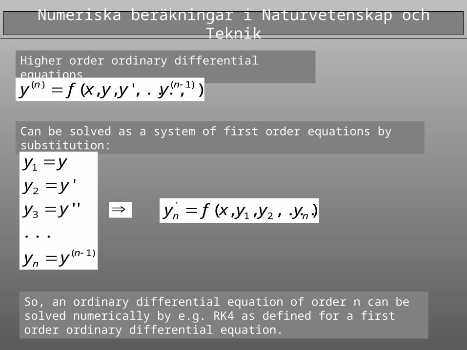
Higher order ordinary differential equations

),...,',,( )1()( nn yyyxfy

Can be solved as a system of first order equations by substitution:

)1(

3

2

1

...

''

'

nn yy

yy

yy

yy

),...,,( 21'

nn yyyxfy

So, an ordinary differential equation of order n can be solved numerically by e.g. RK4 as defined for a first order ordinary differential equation.


condition on y’

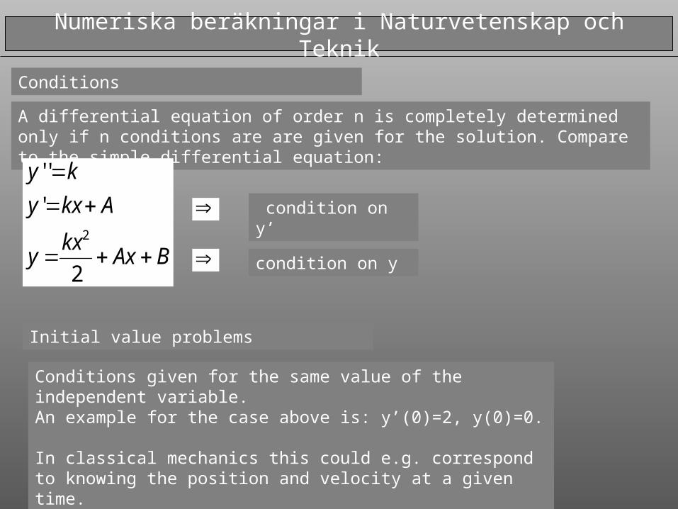
Conditions

A differential equation of order n is completely determined only if n conditions are are given for the solution. Compare to the simple differential equation:

BAxkx

y

Akxy

ky

2

'

''

2

Initial value problems

condition on y

Conditions given for the same value of the independent variable.An example for the case above is: y’(0)=2, y(0)=0.

In classical mechanics this could e.g. correspond to knowing the position and velocity at a given time.


Boundary value problems

In this case one knows the value of the function (and/or its derivatives) for different values of the independent variable. An exemple from physics is the case of a second order differential equation :

)(,)(),',,('' byayyytfy

There are several ways of solving this problem numerically. A simple method is to transfer the problem to become an initial value problem:

)(',)(),',,('' ayayyytfy

and find values for γ that gives solutions that ”shoot over” or ”under” the boundary value in point b. The value forγ which gives a value for y(b) within a given accuracy from βis then solved for. This method is called the “shooting method”. See page 329…


Bounary value problem

)(ay

)(by

say )('

2)( by

1)( by

2)(' ay

1)(' ay


Boundary value problem

nn byay

byay

byay

byay

)()('

...

)()('

)()('

)()('

33

22

11

nnby

by

by

by

),(

...

),(

),(

),(

32

22

11

dvs


Boundary value problem

)(by

s


Exemple; solve with Euler’s method and RK4 and study precision

1)0(, yxydx

dy2/2xey Note that the

solution is:

…possibly another function


Example, second order equation transferred to system

1)0('

1)0(

1''

y

y

y


Exemple, boundary value problem

)(1

'' xfk

T

10)0( T 10)10( T

)sin(53)( xxxf

Documents

Numeriska beräkningar i Naturvetenskap och Teknik 1. Numerical differentiation and quadrature Discrete differentiation and integration Trapezoidal and