Numerical Treatments of Slipping/No-Slip Zones in Cold

HAL Id: hal-01247908https://hal-mines-paristech.archives-ouvertes.fr/hal-01247908

Submitted on 23 Dec 2015

HAL is a multi-disciplinary open accessarchive for the deposit and dissemination of sci-entific research documents, whether they are pub-lished or not. The documents may come fromteaching and research institutions in France orabroad, or from public or private research centers.

L’archive ouverte pluridisciplinaire HAL, estdestinée au dépôt et à la diffusion de documentsscientifiques de niveau recherche, publiés ou non,émanant des établissements d’enseignement et derecherche français ou étrangers, des laboratoirespublics ou privés.

Numerical Treatments of Slipping/No-Slip Zones in ColdRolling of Thin Sheets with Heavy Roll Deformation

Yukio Shigaki, Rebecca Nakhoul, Pierre Montmitonnet

To cite this version:Yukio Shigaki, Rebecca Nakhoul, Pierre Montmitonnet. Numerical Treatments of Slipping/No-SlipZones in Cold Rolling of Thin Sheets with Heavy Roll Deformation. Journal of Fuel and Lubricants,2015, 3 (2), pp.113-131. �10.3390/lubricants3020113�. �hal-01247908�

https://hal-mines-paristech.archives-ouvertes.fr/hal-01247908

https://hal.archives-ouvertes.fr

Lubricants 2015, 3, 113-131; doi:10.3390/lubricants3020113

lubricants ISSN 2075-4442

www.mdpi.com/journal/lubricants

Article

Numerical Treatments of Slipping/No-Slip Zones in Cold Rolling of Thin Sheets with Heavy Roll Deformation

Yukio Shigaki 1,†, Rebecca Nakhoul 2,† and Pierre Montmitonnet 2,†,*

1 Federal Centre of Technological Education of Minas Gerais (CEFET-MG), Belo

Horizonte Unit—Campus II, Amazonas Avenue, 7675—CEP 30510-000—Belo Horizonte/MG,

Brazil; E-Mail: [email protected] 2 Centre de Mise en Forme des Matériaux (CEMEF), MINES ParisTech, PSL Research University,

CNRS UMR 7635, CS 10207 Rue Claude Daunesse, Sophia Antipolis Cedex, 06904, France;

E-Mail: [email protected]

† These authors contributed equally to this work.

* Author to whom correspondence should be addressed;

E-Mail: [email protected];

Tel.: +33-04-9395-7414; Fax: +33-04-9238-9752.

Academic Editor: Jeffrey L. Streator

Received: 22 December 2014 / Accepted: 6 March 2015 / Published: 2 April 2015

Abstract: In the thin sheet cold rolling manufacturing process, a major issue is roll elastic

deformation and its impact on roll load, torque and contact stresses. As in many systems

implying mechanical contact under high loading, a central part is under “sticking friction”

(no slip) while both extremities do slip to accommodate the material acceleration of the

rolled metal sheet. This is a crucial point for modeling of such rolling processes and the

numerical treatment of contact and friction (“regularized” or not), of the transition between

these zones, does have an impact on the results. Two ways to deal with it are compared

(regularization of the stick/slip transition, direct imposition of a no-slip condition) and

recommendations are given.

Keywords: strip rolling; modeling; Finite Element Method; Slab method; slip;

friction; regularization

OPEN ACCESS

Lubricants 2015, 3 114

1. Introduction on Strip Rolling Models, Roll Deformation and the Role of the Friction Stress

Rolling is one of the most important metal manufacturing processes. Starting from continuously cast

slabs, steel is first hot rolled then cold rolled. This latter stage is the one of interest in this paper. As the

material is hard and thin, large contact pressures result in significant roll deformation, which has a major

impact on the process control and on strip geometry [1]. The most impacted characteristics are thickness

profile and flatness defects (see Figure 1) in the case of thin cold rolled flat products, named strips

between 0.1 and 1 mm thick, and foils below 100 µm. In the present paper, where the focus is on friction

models and their consequences, it is sufficient to work with 2D models in a longitudinal cross section,

where strains and stresses are assumed constant along the width direction. In this plane, the elastic roll

deformation problem is called roll flattening.

Figure 1. Schematic representation of the rolling process, showing the roll stack (work roll

(WR), back-up roll (BUR)) and thin strip with typical flatness defects.

1.1. Elastic Roll Deformation Modeling

It is important to realize that a concentrated line loading on a cylinder results in a singular

solution [2]. As a rolling mill roll is highly loaded on a very small part of its periphery, the problem is

not singular but very stiff; however, simple as it may look, it remains an open one.

First estimations of roll deformation were based on the assumption of a quasi-Hertzian contact stress

field (elliptical profile), from which Hitchcock’s formula [3] was derived. It allowed calculating an

equivalent, increased roll radius, which was then used in most of the early rolling models, such as the

Bland and Ford model [4]. Roll deformation was coupled to strip deformation in an iterative way: plastic

or elastic-plastic strip deformation analysis gives a stress profile, which is applied on the roll to give the

deformed roll radius, which is used in next iteration of strip model, etc.

The limitation of Hitchcock’s formula for highly loaded contacts such as found with hard, thin strip

was soon recognized: for large roll deformation, the iterative process described above fails to converge.

Roll radius is increased by the roll load; this makes the contact length longer, which makes the load

grow, which increases the roll radius in an endless process. It has been estimated that whenever the

calculated deformed roll radius reaches the double of the initial one, the results are suspect and for still


higher ratios, divergence may occur [5]. Therefore, much more precise methods were developed to show

that indeed non-circular arc roll deformation models were necessary:

First the Influence Function Method initiated by Jortner et al. [6] and its numerous variants, still

in use today.

Then the Finite Element Method (FEM) introduced by Atreya and Lenard [7] and

Montmitonnet et al. [5], which is now practically abandoned in 2D models due to its much higher

cost. It subsists in 3D rolling models [8] as an alternative to the IFM, which becomes quite

complex in this case.

1.2. Plastic Strip Deformation Modeling and Coupling with Roll Deformation

As for the strip, its elastic-plastic deformation 2D analysis is most of the time based on the Slab

Method (SM). It assumes (i) no dependence of stress and strain on the thickness coordinate either and

(ii) the (Oxyz) frame is the principal frame everywhere, i.e., no shear strains and stresses need to be

considered. The latter assumption is sometimes relieved using Orowan’s model to include an

approximation of shear effects [9]. In 3D, the FEM is used most of the time as the SM is difficult to

extend rigorously in this case.

The roll/strip model coupling technique is essential. The iterative process described above often fails

to converge if no precautions are taken. This is why alternatives have been proposed, based on conjugate

gradient [10] or one-domain FEM computation with internal discontinuity—the roll-strip interface [11].

However the fixed point iterative technique remains the only one in use. The solution to convergence

problems in severe cases relies on relaxation: only a small fraction of the roll surface displacement

calculated at current iteration is used to increment roll shape for next iteration. Recent models propose

adaptive management of the relaxation coefficient, as a function of the convergence performance during

the last few iterations [12,13].

Difficult convergence is related to the normal stress peak found near the “neutral point” where sliding

direction reverses. Indeed, due to incompressibility conjugated with the necessary material acceleration

as the thickness reduction proceeds, the relative velocity is negative on the entry side and positive on the

exit side. This peak can be so sharp as to promote a “trough” in the elastically deformed roll profile, i.e.,

the gap (=the strip thickness) locally re-increases in the central part. This phenomenon, of the order of a

micrometer or less, is now thought to be real [14]. It makes the convergence particularly difficult as the

strip may fall back temporarily in the elastic unloading regime. This is why Matsumoto [12], following

Fleck and Johnson [15], sets a limit to the shape, assuming that the roll gap is at most parallel in the

central part: dt/dx = 0; dt/dx > 0 is forbidden before contact exit (t is the strip thickness, x the abscissa).

1.3. The role of Friction: Regularization

Such a sharp peak of normal stress is strongly dependent on the friction stress in the neighborhood.

In fact, it is easy to show through the equilibrium equations that when rolling thin strips, the major part

of the stress is due to friction:

∂σ∂

~∂σ∂

∂σ∂

(1)


σ is the Cauchy stress tensor, x being the rolling direction and y the normal direction. Figure 2 illustrates

the impact of friction on the normal and tangential stress profiles, on the roll-deformed shape and on the

sliding velocity profile. A very thin steel strip is taken as an example, 0.3 mm reduced to 0.21 mm using

600 mm diameter rolls. When friction increases from µ = 0.02 to µ = 0.035, the roll load, which is the

integral of the normal stress profile, is multiplied by ca. 3.5 and a central flat, no-slip region appears.

Figure 2. Impact of Coulomb friction coefficient µ on mechanical variables in thin strip cold

rolling. From left to right and top to bottom, profiles of the normal stress, the friction stress,

the deformed roll and the sliding velocity (compare with similar figures in [15]).

The way the friction stress model is implemented is therefore critical to the precision of the rolling

model. A correct friction model must include a threshold, a stick-slip transition in the form:

| | if 0 slip

| | if 0 stick (2a,b)

(p,q) are, respectively, the normal and friction stress, vs is the sliding velocity, qc a threshold stress

for sliding, to be specified by a friction law. Though the friction factor model is certainly preferable

under high pressures as found in thin strip rolling, most authors use Coulomb friction i.e., qc = µ·p:

| | μ if 0 slip

| | μ if 0 stick (3a,b)


The stick condition |q| < µp results in a decrease of the friction stress, therefore a decrease of the

normal stress according to Equation (1). This condition can be met in very highly loaded cases in the

central part where pressure is so high as to block sliding. The corresponding reduction of hydrostatic

pressure blunts the normal stress peak and reduces the local roll deformation. As a consequence,

convergence is made easier—by a real, physical effect. However, some models impose sliding to avoid

dealing with the complexity of the stick-slip transition. Such models may have a convergence problem.

Some solve it by introducing a regularization of friction, to decrease it artificially in the critical area

around the neutral point. It consists in smoothing the stick-slip “step” function by multiplying qc by a

continuous and differentiable function e.g., [11]:

| | μ . (4)

K is the regularization factor. Its choice (with respect to the expected values of the sliding velocity)

is essential to regularize the mathematical treatment without transforming too much the physical problem.

This trick is most useful in the FEM where the derivative of friction with respect to sliding velocity or

displacement is needed to build the stiffness matrix. This derivative is infinite at stick/slip transition vs =

0 if the step function is kept. But regularization of friction is also used in the SM context.

Note that Sutcliffe and Montmitonnet [16] use a second type of friction regularization for the extreme

case of Al thin foil rolling, using a slope-dependent (dy/dx) term.

1.4. Purpose and Organization of the Paper

The main intention of this paper is to draw attention to the capabilities and risks of the friction

regularization technique, by quantifying the impact this “numerical trick” may have on the stresses, on

roll deformation and on rolling load. Comparison with a non-regularized formulation with an adequate

treatment of the stick-slip transition will lead to recommendation on the choice of K. It must be

emphasized that these effects are maximized here by selecting thin, hard strip rolling as the test

case—but this is where regularization is useful indeed. Two mathematical formulations of the strip

rolling process will be addressed, the Slab Method (SM) and a Finite Element Model (FEM). The goal

is not to describe them in details or to compare them either; this has been done a number of times in the

past. The test cases are such that we do not expect much difference between them anyway. The purpose

is to show that the behavior of the friction regularization technique is independent of the type of model,

provided it is implemented correctly.

First, the models are described in Section 2, starting with the Slab Method (SM) then the Finite

Element Model (FEM). In Section 3, the impact of regularization on contact stresses, relative velocity

and roll deformation are presented and shown important in thin strip rolling whatever the mathematical

formulation of the problem. Section 4 discusses the choice of the regularization factor, and the extension

of its formulation to investigate friction laws with different static vs. dynamic friction coefficients.


2. Models Description

2.1. Slab Method-Based Model

2.1.1. Stress Field in the Strip

The formulation presented next is taken mainly from the work by Le and Sutcliffe [17].

The constitutive model is elastic-plastic work-hardening. According to the standard Slab Method, it is

assumed that strain and stresses do not vary in the thickness direction, i.e., are independent of y.

The equilibrium of forces applied to the slab (Figure 3) in the rolling direction writes:

dσd

σ 2 0 (5)

where x is the coordinate in the rolling direction, t is the strip thickness, σ is the tensile stress in the

rolling direction, p is the interface pressure and q is the shear stress.

Figure 3. Symbols used in the equations of slab method.

Deformation starts with an elastic compression at onset of contact. Stresses grow and, when the yield

condition is met, plastic deformation occurs, under slip condition as the strip speed increases. As in Le

and Sutcliffe [17], a central flat, sticking zone may occur under higher loads; conditions for this are

described below. In this case, a second plastic reduction zone with slip will follow. In all cases, a final

elastic unloading zone bounds the contact, starting at the point of minimum thickness xd

(Figure 4).


Figure 4. Deformed arc and sticking region ((CPZ) Contained Plastic Zone).

The equations governing the different zones are given hereafter.

(a) In the plastic slip region, the equilibrium Equation (5) is solved together with the elastic-plastic constitutive model. A Tresca yield criterion is assumed: p + σ = Ys (Ys is the plane strain yield stress of the strip), giving, once reported into Equation (5):

dd

dd

2 dd

(6)

Assuming a constant Coulomb friction coefficient μ, friction stress q, wherever sliding is present, is

given by:

μ (7)

where the positive sign is used for the backward slip at entry and the negative sign for the forward slip

on the exit side. In case regularization is applied, this equation can be rewritten as:

μ ..

(8)

Note that here, Vroll, the work roll velocity, has been introduced to make the regularization coefficient

(now Kreg) non-dimensional. The slip velocity vs can be expressed using the volume conservation

principle. Neglecting elastic compressibility:

1 (9)

tn and tx are the thickness of the strip at the neutral point and at point x, respectively.

(b) In the elastic zones at entry and exit of the roll bite, where slip necessarily takes place, the

elastic constitutive equations and the equilibrium equation are reprocessed according to Le and

Sutcliffe [17]:

dd

≅∗ dd 1

2 (10)


(c) In the contained plastic zone (CPZ), the pressure gradient and shear stress for roll and strip are

calculated by imposing the no-slip condition, giving, instead of Equations (5) and (8):

dd

∗ dd

1 21

dd

(11)

21 21

1dd

dd

∗

2dd

(12)

2 41

1 21

∗

∗ (13)

In the case of the problems addressed in this paper, both rolls and strip are made of steel, i.e.,

νs = νR and Es* = ER*, so that C1 = (1 − ν)/(1 − 2ν) ≈ 1.8 and Equations (11,12) are simplified as:

dd

∗ dd

dd

(14)

∗

2dd

(15a)

Finally, Ys is negligible (≈0.3%) compared with the other term in Equation (15), hence: ∗

2dd

(15b)

This no-slip zone starts where q(x) given by Equation (15b) first crosses the curve q(x) for slipping

condition Equations (6–9) and ends at the second intersection point. This procedure has been developed

to prevent the local thickness of the strip from re-increasing inside the roll bite due to too high

roll deformation.

All the equations are integrated by a Runge-Kutta method of order 4 (RK4), using typically

3000 slabs (space integration steps) for each zone.

2.1.2. Work Roll Deformation Equations

The work roll deformation equations applied in this work were developed by Meindl [18] and further

applied for temper rolling model by Krimpelstätter [14].

A sufficient approximation for the cases dealt with here consists in taking into account radial

displacement under the effect of a radial loading (Figure 5), although all four terms can be addressed,

orthoradial as well as radial in terms of stress as well as displacement. Krimpelstätter [14] claims that

orthoradial terms are necessary for very small reduction (temper-rolling).


Figure 5. Principle and symbols for the influence functions method [14].

For a uniform distribution of compressive stress of small angular extension α, the radial work roll

surface displacement is given analytically for a generalized plane strain state by: for Θ (i.e., outside the load area)

Θπ1 υ

2ν

1 ν1 cos Θ α sin Θ α

Θ α2

1 υ2 1 ν

1 cos Θ α

sin Θ αΘ α2

4π

(16a)

for Θ α:

Θ2

11

1 2 Θ α Θ α

π1 sin Θ α

Θ α2

sin Θ αΘ α2

4π

(16b)

for Θ2:

Θ 12 1

1 cos Θ α sin Θ αΘ α2

π1

2 11 cos Θ α

sin ΘΘ2

4π

(16c)

The deformation of the roll for any general distribution of pressure can then be calculated through the

superposition principle.

Note that these influence functions are developed for a diametrically symmetric loading (Figure 5).

This is not exactly the case of strip rolling, since the work-roll/back-up roll contact is shorter and

therefore under higher contact stress than the strip/work roll contact. However, the contact length (a few


mm) is much smaller than the roll diameter (typically 400 to 600 mm in cold rolling). Hence, thanks to

Saint-Venant’s principle, only the resultant load at work roll/back-up roll contact needs to be exact, not

its distribution. The precision of the solution is not impaired.

Displacement is calculated on a roll fraction roughly twice as long as the arc of contact, divided into

200 intervals so that α = 2.7 × 10−4 radian.

2.1.3. Numerical Implementation

Figure 6 shows the flow chart of the global numerical scheme. Some points are detailed hereafter, a

more complete explanation can be found in Le and Sutcliffe [17]. The model is iterative with two main

loops: the global loop and the Neutral Point loop.

Figure 6. Global flow chart of the Slab Method model.

a—In the global cycle, the thickness distribution and the pressure are calculated. The process is

considered converged when:


max| 2 1 | (17)

where tolerance tol = 0.01 t1 (entry strip thickness) typically. A relaxation factor Rt is used for both

thickness and pressure profiles:

updated pressure = Rt current pressure + (1 − Rt) previous pressure (18)

In the applications shown here, Rt ranges from 0.1 to 0.5 (0.1 for the most severe cases). An analogous

expression is applied for the thickness profile.

b—In the neutral point cycle, the neutral point is calculated so as to satisfy:

σ(xe) = σ2 (19)

σ2 is the (given) front tension stress, xe is the contact exit abscissa (Figure 4). Starting the stress

integration from σ = σ1 (the back tension stress) at x = xa, σxe) changes with the position xN of the neutral

point where the sign of q is changed in Equation (7). Using a secant method, the neutral point is found

in general in three or four steps. For more stringent situations, though, the tolerance for the value of the

resulting exit tension stress must be chosen larger in the initial iterations.

2.2. FEM-Based Model

The model used is based on two items:

- A 3D implicit FEM software called Lam3, fully described by Hacquin [19,20]. It is used here

in its steady state option based on streamlines. The integration of the elastic-plastic constitutive

model uses the radial return technique; the compatibility with steady state modeling and

the streamline method is ensured through the ELDTH formulation (Eulerian-Lagrangian

with Heterogeneous Time step). The software uses 8-node hexahedra with reduced pressure

integration. Steady state allows adapted refinement in critical locations (bite entry and exit).

Thermo-mechanical coupling is not activated here.

- A 3D semi-analytical elastic roll deformation model called Tec3, fully described in

Hacquin et al. [21]. It combines roll bending based on Timoshenko’s beam model, roll flattening

based on Boussinesq equations for a semi-infinite solid arbitrarily loaded on its surface, Hertz

contact theory for the work roll/back-up roll contact. End effects for the complex geometry and

boundary conditions of the roll barrel edge have been corrected by analytical expressions derived

from extensive FEM comparisons. All equations are discretized by a 3D influence function

method. Due to the unknown work roll/back-up roll contact areas, the resulting equations are

non-linear and are solved using a Newton-Raphson scheme.

Coupling between the two models is performed by a fixed-point technique with relaxation.

Here, the combined model is used in 2D plane strain, obtained by (1) embedding one layer of elements

between two symmetry planes parallel to the rolling direction; and (2) imposing an infinite stiffness in

the roll deformation model for bending terms only. In this way, a solution equivalent to the 2D model of

Section 3.1 is obtained.


3. Influence of the Regularization Parameter on Rolling Process Mechanics

The parameters used in this work are shown in Table 1, those of the friction models in Table 2.

Table 1. Description of the rolling pass investigated in this paper.

Variable Value

Inlet/exit thickness, t1/t2 0.355 mm/0.252 mm Work roll diameter 555 mm Work roll velocity 20.482 m·s−1

Back/front tension stress, σ1/σ2 170 MPa/100 MPa Young’s modulus (roll and strip) 210 GPa

Poisson’s ratio (roll and strip) 0.3 Flow curve 470.5 175.4ε 1 0.45e . 25 (MPa)

Accumulated strain (prior to the pass investigated) 2.05

Table 2. Non-dimensional parameters of the friction models.

μ 0.02; 0.04 Kreg (Slab Method) 10−2; 3.16 × 10−3; 10−3

Kreg (FEM) 10−1; 10−2; 3.16 10−3; 10−3

Note that Kreg = 10−1 is not used in Section 3.2 (SM) as Section 3.1 (FEM) will show this value to be

too large.

3.1. Impact of Friction Regularization: FEM

Figure 7 pictures the evolution of the friction stress profile with Kreg in the range of 10−3–10−1 for a

moderate friction coefficient of µ = 0.020. Clearly, too high Kreg, of the order of, or higher than, the

typical vs/Vroll, completely changes the friction stress pattern, and therefore all the mechanics of the

rolling process. The roll load F is 10.2 MN·m−1 for Kreg = 10−3, 9.59 MN·m−1 for Kreg = 10−2 and

7.47 MN·m−1 for Kreg = 10−1.

Figure 7. Impact of regularization parameter Kreg on normal (left) and friction stress (right).

Coulomb friction coefficient µ = 0.020.


This emphasizes the danger of this technique if introduced without careful control with numerical

reasons in mind. On the contrary, lower values respect the physics of Coulomb’s friction. They have a

limited, local action in the vicinity of the neutral point, relieving excessive stress there and facilitating

the convergence of the roll deformation coupling. Too low values may, however, leave one with too stiff

a problem, jeopardizing convergence.

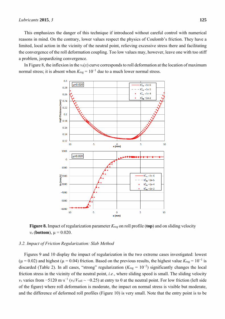
In Figure 8, the inflexion in the vs(x) curve corresponds to roll deformation at the location of maximum

normal stress; it is absent when Kreg = 10−1 due to a much lower normal stress.

Figure 8. Impact of regularization parameter Kreg on roll profile (top) and on sliding velocity

vs (bottom), µ = 0.020.

3.2. Impact of Friction Regularization: Slab Method

Figures 9 and 10 display the impact of regularization in the two extreme cases investigated: lowest

(µ = 0.02) and highest (µ = 0.04) friction. Based on the previous results, the highest value Kreg = 10−1 is

discarded (Table 2). In all cases, “strong” regularization (Kreg = 10−2) significantly changes the local

friction stress in the vicinity of the neutral point, i.e., where sliding speed is small. The sliding velocity

vs varies from −5120 m·s−1 (vs/Vroll ~ −0.25) at entry to 0 at the neutral point. For low friction (left side

of the figure) where roll deformation is moderate, the impact on normal stress is visible but moderate,

and the difference of deformed roll profiles (Figure 10) is very small. Note that the entry point is to be


found at y = 0.1175 mm. The rolling force, which is practically the integral of the vertical stress profile,

varies between 10.1 MN·m−1 for the non-regularized case and 9.68 MN·m−1 for Kreg = 10−2 (−4%) for

the low friction case (µ = 0.020). For µ = 0.04, it increases by 6%, from 29.90 MN·m−1 without

regularization to 31.6 MN·m−1 for Kreg = 10−2.

The high friction case (µ = 0.04) calls for three comments. First, the magnitude of the normal stress,

more than twice as high compared with µ = 0.02, illustrates the very high sensitivity of such thin strip

configurations. The friction stress is therefore up to four times larger (µ × 2 and p × 2), and the shape of

the stress profiles is distorted by the roll-deformed profile. Second, the impact of regularization is the

same as in the previous case. In the central, contained plasticity zone where the roll profile is flat, the

friction stress drops considerably due to the no-slip condition Equation (2b). This effect is also well

captured by the regularized friction model. Third, comparing results for non-regularized and “little

regularized” (Kreg = 10−3) models, it is found that the normal and tangential stresses with regularized

friction are larger (Figure 9). This is surprising since Equation (4) suggests that friction stresses decrease

by the regularization. However, it is important to note that in the Contained Plastic Region (CPZ), a

change in the treatment of stress integration is introduced, replacing Equation (6) by Equations (14) and

(8) by Equation (15b)—see Section 3: as shown by the roll profiles, this has an effect on all aspects of

the contact mechanics.

4. Discussions

4.1. Importance of Friction Regularization and Choice of Kreg

The introduction of friction regularization, in the SM context, just aims at improving convergence in

critical cases. Critical cases are those where a significant “neutral zone” under (quasi-) sticking condition

develops, leading to the coexistence of sticking and slipping zones. This happens both for very low

reduction, the so-called “temper rolling” of steels, and for heavily loaded case, i.e., high reduction of

thin strips of hard metal.

Figure 9. Cont.

-10 -5 0 5 100

500

1000

1500

Nor

mal

str

ess

(MP

a)

x (mm)

non reg.

K2 = 1e -6

K2 = 1e -5

K2 = 1e -4

-10 -5 0 5 100

500

1000

1500

2000

2500

3000

3500

Nor

mal

str

ess

(MP

a)

x (mm)

non reg.

K2 = 1e -6

K2 = 1e -5

K2 = 1e -4


Figure 9. Impact of friction regularization on mechanical variables in thin strip cold rolling,

Slab Method. (Left) µ = 0.020; (right) µ = 0.040. From (top) to (bottom), profiles of the

normal stress, of the friction stress.

Figure 10. Impact of friction regularization on mechanical variables in thin strip cold rolling,

Slab Method. (Left) µ = 0.020; (right) µ = 0.040. From (top) to (bottom), profiles of the

deformed roll and of the sliding velocity.

-10 -5 0 5 10-30

-20

-10

0

10

20

30T

ang

enti

al s

tres

s (M

Pa)

x (mm)

non reg.

K2 = 1e -6

K2 = 1e -5

K2 = 1e -4

-10 -5 0 5 10-150

-100

-50

0

50

100

150

Tan

gen

tia

l str

ess

(MP

a)

x (mm)

non reg

K2=1e-6

K2=1e-5

K2=1e-4

-10 -5 0 5 100.12

0.14

0.16

0.18

0.2

0.22

0.24

0.26

0.28

0.3

Hal

f-th

ickn

ess

(m

m)

x (mm)

non reg.

K2 = 1e -6

K2 = 1e -5

K2 = 1e -4

-10 -5 0 5 100.12

0.13

0.14

0.15

0.16

0.17

0.18

0.19

0.2

0.21

Hal

f-th

ickn

ess

(m

m)

x (mm)

non reg.

K2 = 1e -6

K2 = 1e -5

K2 = 1e -4

-10 -5 0 5 10-0.6

-0.5

-0.4

-0.3

-0.2

-0.1

0

0.1

Vsl

idin

g/V

roll

x (mm)

K2 = 1e -6

K2 = 1e -5

K2 = 1e -4

-10 -5 0 5 10-0.35

-0.3

-0.25

-0.2

-0.15

-0.1

-0.05

0

0.05

0.1

Vsl

idin

g/V

roll

x (mm)

K2 = 1e -6

K2 = 1e -5

K2 = 1e -4


Both are characterized by large roll elastic deformation with a central flat zone around the neutral

point, rather similar to the shape of the solid surfaces in Elasto-Hydrodynamic Lubrication (EHL)—see

Fleck and Johnson [15]. This similarity characterizes problems with heavy loadings where the solution

is dominated by the elastic sub-problem rather than the flow of the fluid or metal in between: by virtue

of their very thinness, a thin oil film or a thin metal strip are stiffer than the roller itself.

For other types of rolling operations, regularization is not necessary in the SM. On the contrary, the

FEM needs regularization because the derivative of the sliding condition τ(vs) has to be computed for

the stiffness matrix and is singular at vs = 0. Regularization by smoothing velocity dependence is

introduced most of the time, although “elastic” regularization has also been proposed [22]: it consists in

adding a small capacity for reversible tangential movement before gross sliding.

Coming back to velocity regularization, as shown above, too small K may lead to convergence

problems in the FEM due to quasi-singular stiffness matrix, or to difficult-to-handle solutions in the SM

(increase of the thickness inside the bite). But too large K may completely alter the physical content of

the friction law, introducing an artificial velocity dependency, and change substantially the mechanical

description of the rolling operation. Table 3 summarizes the impact of Kreg on the roll load and the neutral

zone length. For the rolling operation investigated, the difference between SM and FEM is not more than

1%. It is clear again that Kreg = 10−1 is inadequate; this is why the study has been restricted to Kreg ≤ 10−2

for SM. Even for Kreg = 10−2, some influence shows, 5% for these particular rolling conditions.

Table 3. Variations of global variables (roll load, length of neutral zone) on Kreg.

Kreg Force (MN/m), FEM,

µ = 0.02 Force (MN/m), SM, µ = 0.02

Force (MN/m), SM, µ = 0.04

Lstick (mm) SM, µ = 0.04

10−1 7.47 MN/m - - - 10−2 9.59 MN/m 9.68 MN/m 31.6 MN/m 5.5 mm

3.16 10−3 10.1 MN/m 10.1 MN/m 33.1 MN/m 6.2 mm 10−3 10.2 MN/m 10.1 MN/m 33.4 MN/m 6.4 mm

Non-regularized - 10.1 MN/m 29.9 MN/m 5.5 mm

A more comprehensive study would be needed, but as a rule of thumb, taking Kreg = 10−2 times the

reduction seems a good compromise for rolling. This means Kreg = 10−3 for 10% reduction and

Kreg = 10−4 for 1% reduction in temper rolling where expected sliding velocities are very low.

It must be emphasized that non-dimensionalizing K into Kreg is important: it is quite difficult to

understand what one is doing and to control its effect otherwise. This is the same as for friction for which,

whatever the friction model, non-dimensional coefficients should always be used, such as Coulomb’s

friction coefficient or the friction factor.

4.2. Generality of the Approach

Although different forms may be proposed for velocity regularization of friction (see Li and

Kobayashi [23] for an alternative), this technique can be used universally, wherever it may be useful and

under conditions such that it does not alter the solution of the problem (see above). This is different from

the models (SM and FEM), which have been used here to address the regularization issue. The SM is

valid for most cases of cold strip rolling, wherever the impact of the neglected shear strains and stresses


is not too strong. This means very low bite angle in rolling. The validity can be extended using the

Orowan enhancement technique [9,12]. However, 2D SM of course cannot deal with intrinsically 3D

problems such as strip profile and flatness or strip lateral widening or shrinking (“spread”). The FEM on

the contrary is universally valid; its limitation to 2D here is purely a restriction to the scope of the paper.

The roll deformation model by the Influence Function Method (IFM), in 2D or 3D, has a great precision

at low cost; it belongs to a very general solution technique in elasticity theory. The one used here is

limited to 4-high or 6-high mills, when all roll centerlines are in a same vertical plane; however, similar

techniques are available for e.g., cluster mills such as Sendzimir mills [24].

4.3. Coupling Regularization with the Static/Dynamic Friction Concept

Finally, this paper compares two ways of dealing with the spatial coexistence of sticking and sliding

zones, a variant of the static/dynamic transition, in the space rather than time domain due to the steady

state character of the mechanism investigated, the strip-roll contact in strip rolling processes.

The regularization technique could offer a way to introduce a difference between static friction (µstat)

and dynamic friction (µdyn). The presently chosen regularization function in Equation (4b) varies

monotonically between 0 for vs = 0 and 1 when vs tends to infinity, but it is easy to provide a function

that starts from 0, reaches asymptotically 1 but has a peak larger than 1 in the vicinity of vs = 0, e.g.,

μ .. ..

(16)

Its slope at vs = 0 is a/b2, the peak is at . 1 1 and:

μμ

112.

1 ⁄

1 ⁄ 1 1 ⁄ (17)

The two parameters allow selecting separately µstat/µdyn and the initial slope or the position of the

peak. Any more convenient function may of course be proposed. The impact of such a variant could be

the subject of future work.

5. Conclusions

Two ways of dealing with the slip/no-slip transition within the roll bite in thin strip rolling have been

presented. In the no-slip, contained plasticity zone, the |q| < µp condition can be enforced by comparing

the on-going friction stress with the one deduced from the no-slip condition added to the dt/dx = 0

condition. As a result, q drops in the static friction zones. The same effects can be reproduced in a simpler

way by introducing regularization. Although minor differences are found due to the algorithmic

complexity of the first method, the shapes of the friction stress profile and the normal stress profile

coincide to less than 1% provided the choice of the regularization parameters is made with care. It must

be large enough not to raise convergence difficulties, small enough to stick to the initial problem, since

too large values are equivalent to a decrease of friction coefficient.


Acknowledgments

The authors wish to thank Coordenação de Aperfeiçoamento de Pessoal de Nível Superior (CAPES)

and Centro Federal de Educação Tecnológica de Minas Gerais for providing Yukio Shigaki international

mobility grant for his stay at CEMEF.

Author Contributions

Yukio Shigaki has developed the slab model NonCirc and run the application to the test cases;

Rebecca Nakhoul has run the test cases using the FEM software LAM3; Pierre Montmitonnet has

supervised this work.

Conflicts of Interest

The authors declare no conflict of interest.

References

1. Roberts, W.L. Flat Processing of Steel; Marcel Dekker: New York, NY, USA, 1988.

2. Johnson, K.L. Contact Mechanics, 1st ed.; Cambridge University Press: Cambridge, UK, 1985.

3. Hitchcock, J.H. Roll neck bearings. Report ASME Res. Comm. 1935.

4. Bland, D.R.; Ford, H. The calculation of roll force and torque in cold strip rolling with tensions.

Proc. Inst. Mech. Eng. 1948, 159, 144–153.

5. Montmitonnet, P.; Wey, E.; Delamare, F.; Chenot, J.-L.; Fromholz, C.; de Vathaire, M.

A mechanical model of cold rolling. Influence of the friction law on roll flattening calculated by a

Finite Element Method. In Proceedings of the 4th International Steel Rolling Conference, Deauville,

France, 1–3 June, 1987.

6. Jortner, D.; Osterle, J.F.; Zorowski, C.F. An analysis of cold strip rolling. Int. J. Mech. Sci. 1960,

2, 179–194.

7. Atreya, A.; Lenard, J.G. A study of cold strip rolling. J. Eng. Mater. Technol. (Trans. ASME) 1979,

101, 129–134.

8. Kim, T.H.; Lee, W.H.; Hwang, S.M. An integrated FE process model for the prediction of strip

profile in flat rolling. ISIJ Int. 2003, 43, 1947–1956.

9. Orowan, E. The calculation of roll pressure in hot and cold flat rolling. Proc. Inst. Mech. Eng. 1943,

150, 140–167.

10. Grimble, M.J.; Fuller, M.A.; Bryant, G.F. A non-circular arc force model for cold rolling. Int. J.

Numer. Methods Eng. 1978, 12, 643–663.

11. Gratacos, P.; Montmitonnet, P.; Fromholz, C.; Chenot, J.-L. A plane strain elastoplastic finite

element model for cold rolling of thin strip. Int. J. Mech. Sci. 1992, 34, 195–210.

12. Matsumoto, H. Elastic-Plastic Theory of Cold and Temper Rolling. In Proceedings of the 8th

International Conference on Technology of Plasticity, Verona, Italy, 9–13 October, 2005.

13. Legrand, N.; Ngo, T.; Suzuki, Y.; Takahama, Y.; Dbouk, T.; Montmitonnet, P.; Matsumoto, H.

Advanced Roll Bite Models for Cold and Temper Rolling Processes. In Proceedings of the Rolling

2013 Conference, Venice, Italy, 10–12 June 2013.


14. Krimpelstätter, K. Non circular arc temper rolling model considering radial and circumferential

displacements. Ph.D. Thesis, Linz University, Linz, Austria, 2005 (In German).

15. Fleck, N.A.; Johnson, K.L. Towards a new theory of cold rolling thin foil. Int. J. Mech. Sci. 1987,

29, 507–524.

16. Sutcliffe, M.P.F.; Montmitonnet, P. Numerical modelling of lubricated foil rolling. Rev. Met. SGM

2001, 98, 435–442.

17. Le, H.R.; Sutcliffe, M.P.F. A robust model for rolling of thin strip and foil. Int. J. Mech. Sci. 2001,

43, 1405–1419.

18. Meindl, W. Roll flattening with consideration of shear contact stress. Ph.D. Thesis, Linz University,

Linz, Austria, 2001 (In German).

19. Hacquin, A. Modélisation Thermomécanique Tridimensionnelle du Laminage: Couplage

Bande—Cylindres (3D Thermomechanical Modelling of Rolling Processes: Coupling Strip and

Rolls). Ph.D. Dissertation, MINES ParisTech, Paris, France, 1996 (In French).

20. Hacquin, A.; Montmitonnet, P.; Guillerault, J.P. A steady state thermo-elastoviscoplastic finite

element model of rolling with coupled thermo-elastic roll deformation. J. Mat. Proc. Tech. 1996,

60, 109–116.

21. Hacquin, A.; Montmitonnet, P.; Guillerault, J.P. A 3D semi-analytical model of rolling stand

deformation with finite element validation. Eur. J. Mech. A (Solids) 1998, 17, 79–106.

22. Van der Lugt, J. A FEM for the Simulation of Thermomechanical Contact Problems in Forming

Processes. Ph.D. Dissertation, Twente University, The Netherlands, 1988.

23. Li, G.J.; Kobayashi, S. Rigid plastic finite element analysis of plane strain rolling. Trans. ASME J.

Eng. Mat. Technol. 1982, 104, 55–64.

24. Ogawa, S.; Hamauzu, S.; Matsumoto, H.; Kawanami, T. Prediction of flatness of fine gauge strip

rolled by 12-high Cluster Mill. ISIJ Int. 1991, 31, 599–606.

© 2015 by the authors; licensee MDPI, Basel, Switzerland. This article is an open access article

distributed under the terms and conditions of the Creative Commons Attribution license

(http://creativecommons.org/licenses/by/4.0/).

Documents

Numerical Treatments of Slipping/No-Slip Zones in Cold