Numerical Simulation of the Lid Driven Cavity Flow … Simulation of the Lid Driven Cavity Flow with Inclined walls Ojo Anthony O., Oluwaleye Iyiola O., Oyewola Miracle O. Abstract

International Journal of Scientific & Engineering Research, Volume 4, Issue 5, May-2013 1681 ISSN 2229-5518

IJSER © 2013 http://www.ijser.org

Numerical Simulation of the Lid Driven Cavity Flow with Inclined walls

Ojo Anthony O., Oluwaleye Iyiola O., Oyewola Miracle O.

Abstract— Numerical experiments on 1-sided and 2-sided lid driven cavity with aspect ratio = 1 and with inclined wall were performed. The Vorticity-Stream Function approach and the Finite Element Method (FEM) available through COMSOL, are first compared and the results are analysed for the model CFD driven cavity case which has no analytical solution. The results obtained from the FEM are also compared with findings from established Lattice Boltzmann Models (LBM) available in literature for similar test cases and the results are seen to be in good agreement. The study using FEM was extended to a cavity with inclined walls and it was found that the primary eddy in a cavity significantly changes and is located in the vicinity of the mid plane of the x-coordinate and above the mid plane of the y-coordinate. Its location is dependent on the particular wall that is inclined, the inclination angle and the Reynolds number (Re). The Bottom Left eddies in a cavity where the lid moves in the direction away from the inclined wall, are suppressed with increasing Reynolds numbers and inclination angles, while the Bottom Right eddies generally grows. A merger of these two eddies is seen to occur at Re = 400 and 𝛉 f = 11.31o in a cavity where the lid moves in the direction of the inclined wall; as both grow with increase in Re and 𝛉 f. The Top Left eddies, typical of flows in a cavity at higher Reynolds number of 2000 were not captured, owing to the unstable solution that results when Re > 600 for the cavity with inclined walls, where 𝛉a and 𝛉 f > 0. But these solutions are significantly affected in a cavity with an inclined right wall and is apparent from the diverging results that emerge at Re = 600 and 𝛉 f ≥ 8.53o. A highly refined mesh in the domain is required to be able to adequately visualize the pair of counter rotating eddies that develop at the sharp and inclined corners at higher Re.

Index Terms— COMSOL, Eddies, Finite Element Methods, Inclined walls, Lid driven cavity, Lattice Boltzmann Model, Vorticity-Stream function

—————————— ——————————

1 INTRODUCTION

ignificant progress has been made in employing numerical methods to solve the Navier Stokes (N-S) equations for

incompressible viscous fluid flow in 2-D and 3-D for different coordinate systems, using methods based on: the vorticity equation, artificial compressibility and pressure corrections. Patanker and Spalding [1] developed an implicit formulation in terms of primitive-variables and this formulation, with ref-erence to numerical stability, has no restrictions on the time step. The pressure correction approach constitutes the well known primitive variable formulations, which are solved us-ing the methods such as SIMPLE, SIMPLER, SIMPLEC, PISO algorithm. Chorin developed the artificial compressibility method for handling viscous incompressible flows [2]. Pujol [2,3] used Chorin method and compared it to a vorticity-stream function approach for a 2-D viscous problem and con-cluded that the vorticity-stream function approach is prefera-ble because only velocity boundary conditions are considered. The vorticity formulations for the N-S equations have been adopted in solving flow problems in place of the primitive variables formulations (u, v and p) owing to their simplicity for 2-D flow, by avoiding the unstable iteration caused by the pressure term [4] and their suitability for vortex dominated

flows [5]. As such, based different methods, several numerical schemes have been developed and extended to the study of steady incompressible flow in a driven cavity. This is because of the search for an efficient numerical method for solving the NS equations is unending. The most popular and most thor-oughly studied methods for obtaining such numerical solu-tions are based on finite difference discretizations [2].

The driven cavity contains an incompressible fluid bounded by a square enclosure and the flow is driven by a uniform translation of top lid and it serves as a means through which any numerical scheme can be validated [6]. The driven cavity is a classical problem which has been solved via various numerical schemes. For example, the solutions to the 2-D N-S equations for a driven cavity flow, using the Vorticity-Stream function approach are widely available, where the equations are discretized using the Finite Difference Method (FDM) and solutions are obtained at discrete points in the computational domain. The Lattice Boltzmann Model has recently been em-ployed in simulating single and multi-phase fluid flows. This model is different from top-down models [7, 8] available as the finite difference, finite volume, and finite element meth-ods, which are based on the discretization of partial differen-tial equations. The Lattice Boltzmann Method (LBM) is based on a discrete microscopic model which conserves desired quantities (such as mass and momentum); then the partial dif-ferential equations are derived by multi-scale analysis (bot-tom-up models) [8]. Begum and Basit [6] demonstrated the validity of LBM for different flows and phase transition pro-

S

———————————————— • OJO, Aanthony O is a lecturer in the Mechanical Engineering Department, Ekiti

State University, Ado-Ekiti, Nigeria. E-mail: [email protected] • OLUWALEYE, Iyiola O(Ph.D) is a Reader and the Acting Head of Department,

Mechanical Engineering Department, Ekiti State University, Ado-Ekiti, Nigeria Email: [email protected]

• OYEWOLA, Miracle O (Ph.D) is a Reader in the Mechanical Engineering De-partment, University of Ibadan, Nigeria. Email: [email protected]

IJSER

http://www.ijser.org/



cess. For their simulation, the D2Q9 model was employed and the reliability of their method was checked by implementing it on test problems such as Plane Poiseuille flow, Planar Couette flow and the Lid Driven Cavity flow. The results obtained from their simulations revealed the capability of the incom-pressible LBM model in handling both steady and unsteady flows. Chen et al [5] designed a LBM based on the Vorticity-Stream function equations and the model was tested with sev-eral benchmark problems especially the lid driven cavity prob-lem and the result were seen to have excellent agreement with other numerical data available.

The Finite Element Methods (FEM) has also been em-ployed in the study of the classical benchmark problem of the driven cavity. Wang et al.[9] solved the stream function-vorticity equations for two-dimensional cavity flow by a new finite element method which uses finite spectral basis func-tions as shape functions for rectangular elements. Simulations for several cases with different Reynolds numbers are per-formed and good agreement was obtained in the comparison between their results with the bench mark solutions. The study of such flows in 3-D has also been carried out. Zunic et al [10] carried out a study on the 3-D lid driven cavity flow by mixed boundary and Finite Element Method. The combination of both numerical techniques was proposed in order to in-crease the accuracy of computation of boundary vorticities, a weak point for a majority of numerical methods when dealing with velocity-vorticity formulation. Lid driven flow in a cubic cavity was computed to show the robustness and versatility of their proposed numerical formulation and the results were found to be in good agreement with established results.

Furthermore, the development of CFD packages has fur-ther enhanced the study of fluid flow and this has been facili-tated by the growing capabilities of computers in terms of hardware and software [11]. Research into the use and en-hancement of numerical schemes available through developed codes peculiar to specific flow problem or a general purpose model adaptable to wide range of flow problems is still in progress and remains unending. Hence, several literatures have covered the study and validation of either experimental results with numerical results or numerical results with other numerical results which employed a different solution proce-dure. The success recorded from these researches have further motivated the use of CFD packages in varying a lot of parame-ters which may be difficult or expensive to carry out using experimental or other numerical methods. These packages have also been used to gain full understanding of flows.

The main motivation of this present study is to carry out numerical experiments to (i) visualize the steady flow field in a 1-sided and 2-sided lid driven cavity of a square domain for different Reynolds numbers using the FEM available through COMSOL; (ii) check the capability of the FEM model for the simulation of the steady flow in the lid driven cavity with oth-

er established procedures from the vorticity-stream function formulations and the Lattice Boltzmann Method. (iii) examine the flow field that results at various inclination of the wall for a 1-Sided lid driven cavity and simulate the infinite series of eddies occurring in steady flows in domains with inclined corners. Lid driven cavity flows are important in many indus-trial processing applications such as short-dwell and flexible blade coaters [12].

2 VORTICITY-STREAM FUNCTION FORMULATIONS As a starting point, consider a steady two-dimensional incom-pressible laminar flow. The N-S equations can be written in vorticity-stream function formulation in dimensionless form as

where the vorticity is given as,

the horizontal velocity, U and vertical velocity, V are given as

and x and y are the Cartesian coordinates. The governing equations above are solved on a grid mesh with 51 x 51 grid points for a square driven cavity using the SOR method and MATLAB codes are used to simulate both a 1 sided and 2 sid-ed lid driven cavity flow. Erturk et. al. [13] cited by Erturk [14] stated that for square driven cavity when fine grids are used, it is possible to obtain numerical solutions at high Reynolds numbers. Figures (1)~(2) shows the schematic of the driven cavity.

.

3 FEM-COMOSL MODEL

The CFD package, COMSOL was employed for simulating the lid driven cavity flow in order to determine the flow parame-

Fig.1: 1-sided Lid Driven

(4) IJSER




ters that emerge under the influence of varying Reynolds numbers. It is pertinent to note that COMSOL runs the Finite Element Method (FEM) for discretisation of the domain and the use of FEM allows momentum conservation in the compu-tational domain. As such, this enables investigation of other parameters that pertain to the flow. The excellent meshing capability of the solver is employed at the sharp corners and an inclined surface so as to capture eddies that develop at those regions. Figures (1)~(3) shows the schematic of the driv-en cavity modelled with COMSOL where the Reynolds num-ber used was evaluated from the expression

and for the 2-sided lid driven cavity,

4 NUMERICAL RESULTS AND DISCUSSIONS In other to establish the rationality of the present model for a lid driven cavity with inclined walls, we first compare the so-lution from the FEM with the vorticity-stream function (V-S) solution for a steady flow. From various literatures examined in this study, it is a consensus that: steady flow is stable for small and reasonable Reynolds numbers. The contour lines for the U-velocity distribution and stream function in the cavity for Re = 10 are illustrated in Figures (4) ~ (6). The highly re-fined mesh and contour lines employed in the FEM solution allow for the capturing of the bottom right corner and bottom left corner eddies (Figure 4d) that develop in the cavity at this

Reynolds number for a 1-sided lid driven cavity. Numerical solutions can be obtained in the computational domain for higher Reynolds numbers when a more refined mesh is em-ployed. Flow in a 2-sided lid driven cavity, with the top and bottom lid moving in parallel or anti–parallel motion, was also simulated using both V-S and FEM approaches and the con-tours obtained for U and , from the simulation are presented. For anti-parallel wall motion (Re1= Re2), where the top and bottom lids move in opposite directions, the U-velocity and contours are symmetric about the mid-plane of the cavity for the y coordinate as shown in Figure 5. A parallel wall motion exists when both walls move in the same direction with the same velocity, Uwall and Re1= -Re2. Figure 6(c) & (d) shows that from a 2D perspective, the streamlines are mirror images about the mid plane of the cavity for the y coordinate.

The locations of the vortices or eddies in a 1-sided lid driven cavity from the present work using the FEM approach is further compared with the LBM used for similar flow ob-tained in literatures. Chen et al. [5] and Patil et al. [17] em-ployed the LBM for simulation of flow in a 1-sided lid driven cavity and the locations of the vortices are presented in Table 1. Furthermore, the locations of the vortices in the cavity from the popular work of Ghia et al.[15] which focused on High-Re solutions of incompressible flow using N–S equations and a multigrid method is also contained in Table 1. The Re covered is 50, 400, 1000 and 2000. The results from this study are in good agreement with other numerical methods employed. From the simulation performed, it is quickly seen from Figures (7)~(10), that in addition to the primary centre vortex or Pri-mary Eddy (PE) a pair of oppositely rotating eddies of much lesser strength is formed in the lower corners (Bottom Right (BR) and Bottom Left (BL)) called the Moffat eddies. This is so because, for a viscous flow near a corner, there exist an infinite series of eddies with decreasing size and intensity [18]. For low Re, the centre of the PE is located at the horizontal mid section of the cavity and at the upper part of the cavity. With an increase in Re, the PE moves towards the centre of the cavi-ty becomes progressively more circular. It is also quickly seen from Figures (7)~(10) that a TL eddy is a flow feature that be-comes apparent at higher Re. For Re ≤ 1000 three eddies (PE, BL, BR) can be found in the cavity and at Re = 2000, a fourth eddy (TL) becomes obvious [5]. Additionally, as Re increases, the BR eddies gradually move left and upward from their loca-tions at low Re.

Given the above justification on the capabilities of the present FEM model, as it allows computation of the position of the primary and corner eddies. In addition to obtaining other characteristics of the steady flow in a lid driven cavity, we ex-tended the study to examine the influence of inclined walls on the flow features within a 1-sided lid driven cavity. Two cases where the top lid moves in the direction: (1) of the inclined right wall (2) away from the inclined left wall (Figure 3) were examined. The angles of inclination employed are 2.86o, 5.71 o,

(a) Anti-Parallel wall motion (b) Parallel wall motion

Fig.2: 2-sided Lid driven cavity

(4)

(a) Lid moves away from (b) Lid moves in direction facing

inclined left wall (LWI) the inclined right wall (RWI)

Fig.3: 1-sided Lid driven cavity with inclined walls

IJSER




8.53o and 11.31o for both cases. The mesh was highly refined in the solver at the inclined and vertical walls for all simulations performed. The solution time for the simulation was between 142 sec – 160 secs varying with increased angle of inclination and Re. The elements employed due to refinement near the walls ranges between 5874 and 6144 elements. The U-velocity distribution along a vertical line passing through the centre of the cavity in a cavity with 𝛉a = 𝛉f = 0o for Re = 50, 200, 400 and 600 is presented in Figure 11 which is at par with literatures on similar subject.

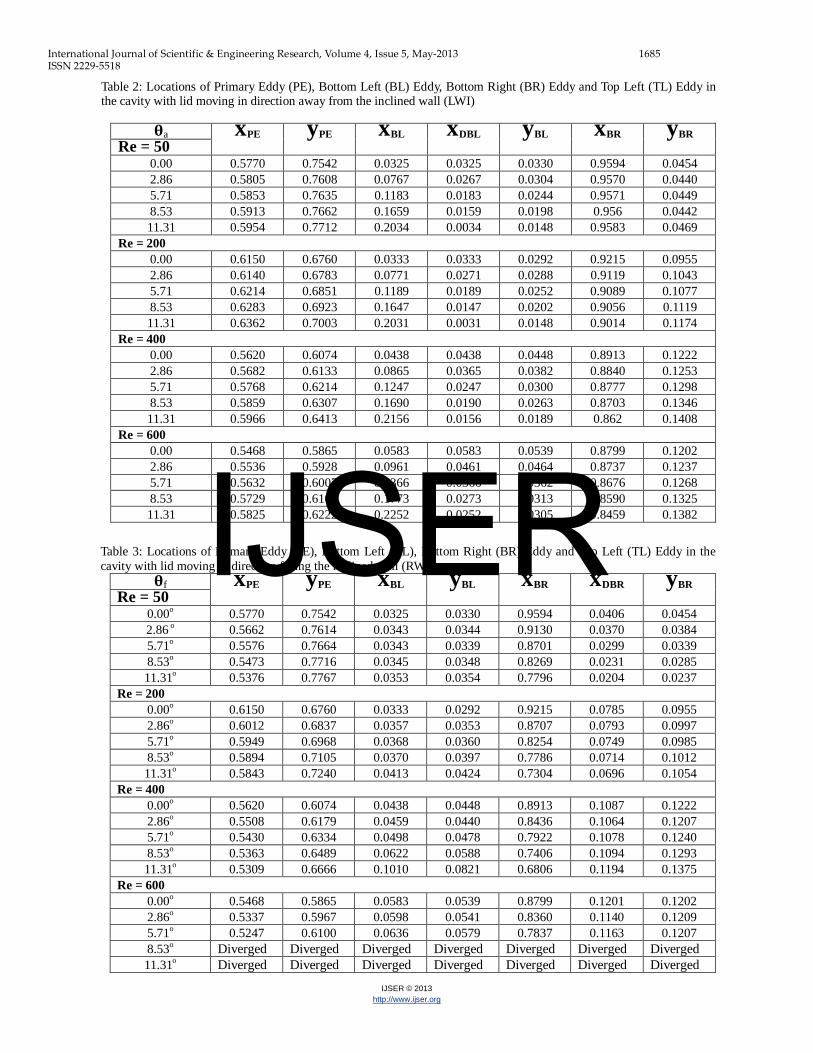
With increasing angles of inclination, for each Re, there is a shift in location of the PE from the position occupied when 𝛉a = 𝛉f = 0. The centre location of the PE, BR, and BL eddies in a cavity where the lid moves in the direction away from the in-clined wall (LWI) are contained in Table 2. The TL eddy that developed at Re = 2000 for a vertical (𝛉a = 0) left wall was not a feature of the flow for various angles of inclination. This is because the numerical solution became unstable at Re > 600 yielding diverging results. Based on the current model em-ployed in terms of maximum 𝛉a, the critical Re is 600. For a square cavity, it was mentioned that with increasing Re, the PE gradually moves towards the centre of the cavity becoming increasingly circular but in general, the influence of inclination causes the x and y-location of the PE to be displaced from the centre. Investigations carried out for all Re and 𝛉a reveal that the position of PE is maintained in the top half of the mid plane of the y-coordinate and for each Re, increasing values of 𝛉a causes a gradually progressive upward shift from the position it occupied at 𝛉a =0o. At each 𝛉a, an increase in Re causes

the PE to move to the right of the mid plane of the x coordi-nate and towards the mid plane of the y coordinate in the cavi-ty. This is unsurprising due to the influence of the displace-ment caused by the inclined wall and the tendency of the PE to gradually proceed to the centre of the cavity, while becoming circular. The contours for the streamlines for the left inclined wall, shows that the formation of the BL eddies are gradually suppressed as a result of the influence of increasing 𝛉a and the primary eddies that develop at each Re. Figures 12 and 13 ((a) ~(c)) shows the suppression of the BL eddies due to wall incli-nation for Re = 50 and 600. This suppression is significant at low Re and is apparent in both horizontal displacement (xDBL) and vertical locations of the BL eddy. For every Re, an increase in 𝛉a causes a suppression of this eddy; as it progressively grows smaller in size. The BR eddy grows with an increase in 𝛉a for every Re. This eddy is as a result of the sharp corner that exists at the vicinity and the greater the Re and the angle of inclination of the left wall, the larger the BR eddy. Figures 12 and 13 shows the , , U- velocity distribution in the cavity having the left wall inclined as 𝛉a = 0 o, 5.71 o and 11.31o for Re = 50 and 600. A vertical line passing through the centre of the cavity when 𝛉a = 𝛉f = 0o was also used to compute the U-velocity distribution for cases of varying wall inclination an-gles. No significant change was noticed in variation of this velocity with changing Re and 𝛉a (Figure 14). However it can be quickly seen from figure 14b that a noticeable change oc-curs at Re = 600 and 𝛉a = 11.31o.

Table 1: Locations of Primary Eddy (PE), Bottom Left (BL) Eddy and Bottom Right (BR) Eddy in the square cavity Re = 50 xPE yPE xBL yBL xBR yBR

Ghia et al.[5,15] - - - - - - Guo et al. [5,16] - - - - - - Patil et al. [5,17] 0.5781 0.7578 0.0468 0.0468 0.9609 0.0546 Chen et al. [5] 0.5796 0.7601 0.0440 0.0440 0.9551 0.0505 Present Work* 0.5770 0.7542 0.0325 0.0330 0.9594 0.0454 Re = 400 Ghia et al.[5,15] 0.5547 0.6055 0.0508 0.0469 0.8906 0.1250 Guo et al. [5,16] 0.5547 0.6094 0.0508 0.0469 0.8867 0.1250 Patil et al. [5,17] 0.5625 0.6133 0.0507 0.0507 0.8906 0.1289 Chen et al. [5] 0.5510 0.6100 0.0500 0.0500 0.8810 0.1298 Present Work* 0.5620 0.6074 0.0438 0.0448 0.8913 0.1222 Re = 1000 Ghia et al.[5,15] 0.5313 0.5625 0.0859 0.0781 0.8594 0.1094 Patil et al. [5,17] 0.5391 0.5703 0.0937 0.0859 0.8750 0.1250 Chen et al. [5] 0.5309 0.5699 0.0899 0.0800 0.8610 0.1180 Present Work* 0.5336 0.5659 0.0771 0.0770 0.8665 0.1138 Re = 2000 Ghia et al.[5,15] - - - - - - Guo et al. [5,16] 0.5234 0.5469 0.0898 0.1016 0.8438 0.1016 Patil et al. [5,17] - - - - - - Chen et al. [5] 0.5205 0.5501 0.0900 0.1010 0.8399 0.1009 Present Work* 0.5240 0.5483 0.0862 0.0998 0.8487 0.1006

IJSER




Table 2: Locations of Primary Eddy (PE), Bottom Left (BL) Eddy, Bottom Right (BR) Eddy and Top Left (TL) Eddy in the cavity with lid moving in direction away from the inclined wall (LWI)

𝛉a xPE yPE xBL xDBL yBL xBR yBR Re = 50

0.00 0.5770 0.7542 0.0325 0.0325 0.0330 0.9594 0.0454 2.86 0.5805 0.7608 0.0767 0.0267 0.0304 0.9570 0.0440 5.71 0.5853 0.7635 0.1183 0.0183 0.0244 0.9571 0.0449 8.53 0.5913 0.7662 0.1659 0.0159 0.0198 0.956 0.0442 11.31 0.5954 0.7712 0.2034 0.0034 0.0148 0.9583 0.0469

Re = 200 0.00 0.6150 0.6760 0.0333 0.0333 0.0292 0.9215 0.0955 2.86 0.6140 0.6783 0.0771 0.0271 0.0288 0.9119 0.1043 5.71 0.6214 0.6851 0.1189 0.0189 0.0252 0.9089 0.1077 8.53 0.6283 0.6923 0.1647 0.0147 0.0202 0.9056 0.1119 11.31 0.6362 0.7003 0.2031 0.0031 0.0148 0.9014 0.1174

Re = 400 0.00 0.5620 0.6074 0.0438 0.0438 0.0448 0.8913 0.1222 2.86 0.5682 0.6133 0.0865 0.0365 0.0382 0.8840 0.1253 5.71 0.5768 0.6214 0.1247 0.0247 0.0300 0.8777 0.1298 8.53 0.5859 0.6307 0.1690 0.0190 0.0263 0.8703 0.1346 11.31 0.5966 0.6413 0.2156 0.0156 0.0189 0.862 0.1408

Re = 600 0.00 0.5468 0.5865 0.0583 0.0583 0.0539 0.8799 0.1202 2.86 0.5536 0.5928 0.0961 0.0461 0.0464 0.8737 0.1237 5.71 0.5632 0.6007 0.1366 0.0366 0.0362 0.8676 0.1268 8.53 0.5729 0.6103 0.1773 0.0273 0.0313 0.8590 0.1325 11.31 0.5825 0.6222 0.2252 0.0252 0.0305 0.8459 0.1382

Table 3: Locations of Primary Eddy (PE), Bottom Left (BL), Bottom Right (BR) Eddy and Top Left (TL) Eddy in the cavity with lid moving in direction facing the inclined wall (RWI)

𝛉f xPE yPE xBL yBL xBR xDBR yBR Re = 50

0.00o 0.5770 0.7542 0.0325 0.0330 0.9594 0.0406 0.0454 2.86 o 0.5662 0.7614 0.0343 0.0344 0.9130 0.0370 0.0384 5.71o 0.5576 0.7664 0.0343 0.0339 0.8701 0.0299 0.0339 8.53o 0.5473 0.7716 0.0345 0.0348 0.8269 0.0231 0.0285 11.31o 0.5376 0.7767 0.0353 0.0354 0.7796 0.0204 0.0237

Re = 200 0.00o 0.6150 0.6760 0.0333 0.0292 0.9215 0.0785 0.0955 2.86o 0.6012 0.6837 0.0357 0.0353 0.8707 0.0793 0.0997 5.71o 0.5949 0.6968 0.0368 0.0360 0.8254 0.0749 0.0985 8.53o 0.5894 0.7105 0.0370 0.0397 0.7786 0.0714 0.1012 11.31o 0.5843 0.7240 0.0413 0.0424 0.7304 0.0696 0.1054

Re = 400 0.00o 0.5620 0.6074 0.0438 0.0448 0.8913 0.1087 0.1222 2.86o 0.5508 0.6179 0.0459 0.0440 0.8436 0.1064 0.1207 5.71o 0.5430 0.6334 0.0498 0.0478 0.7922 0.1078 0.1240 8.53o 0.5363 0.6489 0.0622 0.0588 0.7406 0.1094 0.1293 11.31o 0.5309 0.6666 0.1010 0.0821 0.6806 0.1194 0.1375

Re = 600 0.00o 0.5468 0.5865 0.0583 0.0539 0.8799 0.1201 0.1202 2.86o 0.5337 0.5967 0.0598 0.0541 0.8360 0.1140 0.1209 5.71o 0.5247 0.6100 0.0636 0.0579 0.7837 0.1163 0.1207 8.53o Diverged Diverged Diverged Diverged Diverged Diverged Diverged 11.31o Diverged Diverged Diverged Diverged Diverged Diverged Diverged

IJSER




The locations of the PE, BL and BR eddies for a 1-sided lid driven cavity with the RWI and in which the top lid moves in the direction of the inclined wall are presented in Table 3. Fig-ures 15 and 16 show the , , U- velocity distribution in the cavity having the left wall inclined as 𝛉f = 0o, 5.71 o and 11.31o for Re = 50 and 400. In general, with increasing 𝛉f, for each Re, the PE is observed to proceed towards the mid plane of the x-coordinate of the cavity but gradually shifts upward away from the mid plane of the y-coordinate of the cavity. Further-more, with increasing Re, for each 𝛉f, the PE moves to towards the mid plane of the x-coordinate and towards the mid plane of the y-coordinate of the cavity. The BL eddy progressively grows with increasing Re and 𝛉f owing to the sharp corner existing at this vicinity. For Re =50, the BR is observed to be small and is suppressed with increasing 𝛉f. This eddy is seen to grow with increasing Re for each 𝛉f. The growth of the BR eddies is apparent from its horizontal displacement (xDBR) and

vertical position with increasing Re and 𝛉f. Owing to the wall inclination and the direction of flow towards this wall, the growth of this BR eddy is significant at Re = 400 and 𝛉f = 11.31o. At this point, a merger is seen to occur between the BL and BR eddies. This merger becomes possible at this Re owing to the increasing 𝛉f. The streamlines at Re = 400 for cases where 𝛉f = 8.53o and 11.31o are presented in Figure 17. At Re = 600 and 𝛉f ≥ 8.53 o the solution in the computational domain becomes unstable as it diverges. In this RWI cavity, the U-Velocity distribution along the same vertical line passing through the centre of the cavity for 𝛉a = 𝛉f = 0o is presented in Figure 18. The influence of increasing Re and 𝛉f is seen to af-fect the flow characteristics in the cavity significantly com-pared to a case of increasing Re and 𝛉a. From Figure 18, it can be quickly noticed that the U-velocity profile along the vertical line of interest is affected, due to the increasing Re, the in-clined Right wall and increasing 𝛉f.

(a) (b)

(c) (d) Fig. 4: 1-Sided Lid driven cavity for Re= 10 (a) V-S FDM – U-velocity (b) FEM: U-velocity (c) V-S FDM – (d) FEM –

(a) (b)

(c) (d)

Fig. 5: Anti-parallel wall motion for a 2-Sided Lid driven cavity for Re= 10 (a) V-S FDM – U-velocity (b) FEM: U-velocity (c) V-S FDM – (d) FEM –

IJSER




(a) (b)

(c) (d)

Fig. 6: Parallel wall motion for a 2-Sided Lid driven cavity for Re= 10 (a) V-S FDM – U-velocity (b) FEM: U-velocity (c) V-S FDM – (d) FEM –

(a) (b)

Fig. 7: 1- Sided Lid driven Cavity for Re= 50 (a) [5] (b) (present work)

(a) (b)

Fig. 8: 1- Sided Lid driven Cavity for Re = 400 (a) [5](b) (present work)

(a) (b)

Fig. 9: 1- Sided Lid driven Cavity for Re = 1000 (a) [5](b) (present work)

(a) (b)

Fig. 10: 1- Sided Lid driven Cavity for Re = 2000 (a) [5](b) (pre-sent work)

Fig.11: U-Velocity distribution along a vertical line through the cen-

tre of the cavity where 𝛉a = 𝛉f = 0o

IJSER




(a) (b) (c)

(a’) (b’) (c’)

(a’’) (b’’) (c’’)

Fig. 12: Lid driven Cavity with Inclined wall for Re = 50;𝛉a = 0o (a) (a’) (a’’) U- velocity 𝛉a = 5.71o (b) (b’) (b’’) U- velocity

𝛉a = 11.31o (c) (c’) (c’’) U- velocity

IJSER




(a) (b) (c)

(a’) (b’) (c’)

(a’’) (b’’) (c’’)

Fig.13: Lid driven Cavity with Inclined wall for Re = 600; 𝛉a = 0o (a) (a’) (a’’) U- velocity 𝛉a = 5.71o (b) (b’) (b’’) U- velocity

𝛉a = 11.31o (c) (c’) (c’’) U- velocity

IJSER




(a) (b) (c)

(a’) (b’) (c’)

(a’’) (b’’) (c’’)

Fig.15: Lid driven Cavity with Inclined wall - Re = 50; 𝛉f = 0o (a) (a’) (a’’) U- velocity 𝛉f = 5.71o (b) (b’) (b’’) U- velocity

𝛉f = 11.31o (c) (c’) (c’’) U- velocity

(a) (b)

Fig.14: U-Velocity distribution in a cavity with inclined wall (a) 𝛉a = 5.71o (b) 𝛉a = 11.31o

IJSER




(a) (b)

(a’) (b’)

(a’’) (b’’)

Fig.16: Lid driven Cavity with Inclined wall - Re = 600 𝛉f = 0o (a) (a’) (a’’) U- velocity

𝛉f = 5.71o (b) (b’) (b’’) U- velocity

(a) (b)

Fig.17: Lid driven Cavity with Inclined wall - Re 400 (a) 8.53o (b) 11.31o

IJSER




Figures (19) ~ (20) shows the influence of Re on the U-velocity profile along the straight line of interest in the LWI and RWI cavities. At Re = 50, for both the LWI and RWI cavities, where 𝛉a = 𝛉f = 5.71o, no significant change is noticeable in the U-velocity distribution along the same vertical line passing through the centre of the cavity for 𝛉a = 𝛉f = 0o. With increas-ing

Re, a small difference is noticeable between the U-velocity profiles of the fluid in the LWI and RWI cavities. The differ-ence is significant at higher Re when 𝛉a = 𝛉f = 11.31o and is obvious from figure 20. This is an indication of the affected flow characteristics in a RWI cavity due to increasing Re and 𝛉a.

(a) (b)

Fig.18: U-Velocity distribution in a cavity with inclined wall (a) 𝛉f = 5.71o (b) 𝛉f = 11.31o

(a) (b)

(c) (d) Fig.19: U’ – velocity profile for 𝛉f and 𝛉a = 5.71o (a) Re = 50 (b) Re = 200 (c) Re = 400 (d) Re = 600

IJSER




5 CONCLUSION

Numerical experiments have been conducted for flow in the lid driven cavity using the FEM on the CFD package, COMSOL and the results obtained were presented. The approach was first vali-dated with other benchmark procedures for a 1-sided and 2-sided lid driven cavity using the V-S approach and LBM. These results are in excellent agreement with the model employed on COMSOL as the contour patterns and locations of the primary and second-ary ‘corner’ eddies are reliable. Flow in a 1-sided cavity with top lid moving in the direction (1) away from the inclined (left) wall (2) facing the inclined (right) wall is then investigated. Various angles of inclinations (2.86o, 5.71o, 8.53o and 11.31o) and Reynolds number Re (50, 200, 400 and 600) were employed. The Primary eddy was noticed to be maintained at the top half of the mid plane of the y-coordinate for respective cases of inclined Left or Right wall. Corner eddies develop at both inclined and sharp cor-ners. With increase in Re and 𝛉a, the BR eddies are suppressed and the BR eddies generally grow. This is in contrast to a case of a

cavity with increased in Re and 𝛉 f, where both BR and BL eddies grow and merge together at a critical Re and 𝛉 f of 400 and 11.31o. The numerical solution yielded unstable results for both cases of inclined walls when Re > 600. The influence of increasing Re and 𝛉f is seen to affect the flow characteristics in the cavity significant-ly as compared to a case of increasing Re and 𝛉a

Nomenclature x = horizontal coordinate y = vertical coordinate U = x- velocity component U’ = dimensionless x- velocity component V = y- velocity component Uwall = velocity of moving lid Re= Reynolds number L = Length of top lid 𝛉a = angle of inclination for left wall for which top lid moves away from 𝛉 f = angle of inclination for right wall for which top lid moves towards PE = Primary eddy BL = Bottom Left

(a) (b)

(c) Fig.20: U’ – velocity profile for 𝛉f and 𝛉a = 11.31o (a) Re = 50 (b) Re = 200 (c) Re = 400

IJSER




BR = Bottom Right TL = Top Left H = Cavity Height XDBL = Displacement of Bottom left eddy from Left wall XDRL = Displacement of Bottom left eddy from Right wall RWI = Right Wall Inclined LWI = Left Wall Inclined

Greek Letters ω = vorticity ψ = stream function ρ = density υ = kinematic viscosity

6 REFERENCES [1] S.V. Patanker, D.B. Spalding, A calculation procedure for heat,

mass and momentum transfer in three-dimensional parabol-ic flows, Int. J. of Heat Mass Transfer, 15, 1787-1806, 1972.

[2] K. A. Salwa, A.F. I. Gamal, S. M. Berlant, 2004, Efficient Nu-merical Solution of 3d Incompressible Viscous Navier-Stokes Equations, International Journal of Pure and Applied Math-ematics Volume 13 no. 3, 391-411, 2004.

[3] A. Pujol, Numerical Experiments on the Stability of Poiseuille Flows of Non-Newtonian Fluids, Ph.D. Dissertation, Univer-sity of Iowa, Iowa City, Iowa, 1971.

[4] Je -Ee Ho (2008) Developing a Convective Code With Vorticity Transport in Upwind Method, Journal of Marine Science and Technology, Vol. 16, No. 3, pp. 191-196, 2008.

[5] S. Chen et al., A new method for the numerical solution of vor-ticity–streamfunction formulations, Comput. Methods Appl. Mech. Engrg. , doi:10.1016/j.cma.2008.08.007, 2008.

[6] R. Begum and A. M. Basit, Lattice Boltzmann Method and its Applications to Fluid Flow Problems, European Journal of Scientific Research, ISSN 1450-216X Vol.22 No.2, pp.216-23. EuroJournals Publishing, Inc. 2008.

[7] D. A. Wolf-Gladrow, Lattice-Gas Cellular Automata and Lat-tice Boltzmann Models, An Introduction, Springer-Verlag Berlin Heidelberg. ISSN 0075-8434 ISBN 3- 540-66973-6, 2000.

[8] J. Kang, The Lattice Gas Model and Lattice Boltzmann Model On Hexagonal Grids, M.Sc. Thesis, Auburn University, Ala-bama, 2005

[9] J.P. Wang, Y. Nakamura, T. W. Li, Computation of Cavity Flow by Finite Element Method with Finite Spectral Shape Func-tion, The 5TH Asian Computaitional Fluid Dynamics Busan, Korea, October 27-30, 2003

[10] Z. Zunic, M. Hribersek, L. Skerget and J. Ravnik, 2006, 3D Lid Driven Cavity Flow By Mixed Boundary And Finite Element Method, European Conference on Computational Fluid Dy-namics, ECCOMAS CFD. TU Delft, The Netherlands, 2006.

[11] W. Ludwig, J. Dziak* CFD Modelling Of A Laminar Film Flow, Chemical and process engineering,2009, 30, 417–430

[12] C.K. Aidun, N.G. Triantaflllopoulos, J.D. Benson, Global sta-bility of a lid-driven cavity with throughflow: flow visuali-zation studies, Phys. Fluids A 3(9) 2081 – 2091 ,1991

[13] E. Erturk, T.C. Corke, C. Gokcol, Numerical Solutions of 2-D Steady Incompressible Driven Cavity Flow at High Reynolds Numbers. International Journal for Numerical Methods in Fluids 48, 747–774. 2005.

[14] E. Erturk, Discussions on Driven Cavity Flow, Int. J. Numer. Meth. Fluids 2009; Vol 60: pp 275-294, 2009.

[15] U. Ghia, K. Ghia, C. Shin, High-Re solutions for incompress-ible flow using Navier–Stokes equations and a Multigrid method, J. Comput. Phys. 48, 387–411, 1982.

[16] Z.L. Guo, B.C. Shi, N.C. Wang, Lattice BGK model for incom-pressible Navier– Stokes equation, J. Comput. Phys. 165 288–306, 2000.

[17] D.V. Patil, K.N. Lakshmisha, B. Rogg, Lattice Boltzmann sim-ulation of lid-driven flow in deep cavities, Comput. Fluids 35, 1116–1125, 2006.

[18] H. K. Moffat, Viscous and resistive eddies near a sharp cor-ner, J. Fluid Mech., 18, pp. 1–18, 1964.

IJSER


Documents

Numerical Simulation of the Lid Driven Cavity Flow … Simulation of the Lid Driven Cavity Flow with Inclined walls Ojo Anthony O., Oluwaleye Iyiola O., Oyewola Miracle O. Abstract