Numerical Simulation of Heat Transfer in Materialswith Anisotropic Thermal Conductivity:

A Finite Volume Scheme to Handle Complex Geometries

Olaf Klein1, Jurgen Geiser1, Peter Philip2

1Weierstrass Institute forApplied Analysis and Stochastics (WIAS)

Berlin, Germany

2University of MinnesotaInstitute for Mathematics and its Applications (IMA)

Minneapolis, USA

IMA Workshop:

New Paradigms in Computation

Minneapolis, March 28–30, 2005

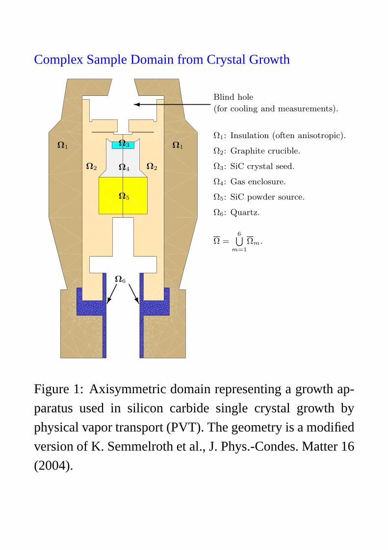
Complex Sample Domain from Crystal Growth

Ω1 Ω1

Ω2 Ω2

Ω3

Ω4

Ω5

AAU

Ω6

Blind hole

(for cooling and measurements).

Ω1: Insulation (often anisotropic).

Ω2: Graphite crucible.

Ω3: SiC crystal seed.

Ω4: Gas enclosure.

Ω5: SiC powder source.

Ω6: Quartz.

Ω =6S

m=1

Ωm.

Figure 1: Axisymmetric domain representing a growth ap-

paratus used in silicon carbide single crystal growth by

physical vapor transport (PVT). The geometry is a modified

version of K. Semmelroth et al., J. Phys.-Condes. Matter 16

(2004).

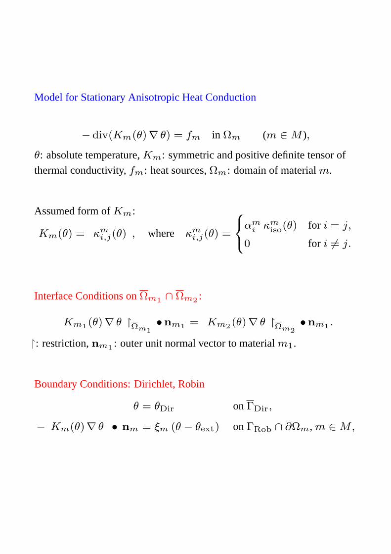
Model for Stationary Anisotropic Heat Conduction

− div(Km(θ)∇ θ) = fm in Ωm (m ∈ M ),

θ: absolute temperature,Km: symmetric and positive definite tensor of

thermal conductivity,fm: heat sources,Ωm: domain of materialm.

Assumed form ofKm:

Km(θ) =ąκm

i,j(θ)ć, where κm

i,j(θ) =

8<:

αmi κm

iso(θ) for i = j,

0 for i 6= j.

Interface Conditions onΩm1 ∩ Ωm2 :

ąKm1 (θ)∇ θ

ć¹Ωm1•nm1 =

ąKm2 (θ)∇ θ

ć¹Ωm2•nm1 .

¹: restriction,nm1 : outer unit normal vector to materialm1.

Boundary Conditions: Dirichlet, Robin

θ = θDir onΓDir,

−ąKm(θ)∇ θ

ć • nm = ξm (θ − θext) onΓRob ∩ ∂Ωm, m ∈ M,

Finite Volume Discretization

Σm = (σm,i)i∈Im conforming triangulation ofΩm satisfying the

constrained Delaunay property: If γ is an interior edge ofΣm, α andβ

the angles opposite toγ, thenα + β ≤ π. If γ ⊆ ∂Ωm is a boundary

edge ofΣm, α the angle oppositeγ, thenα ≤ π/2.

V (σm,i) =ľvm

i,j : j ∈ 1, 2, 3ł: Set of vertices.

V :=S

m∈M, i∈ImV (σm,i).

ωv :=ľx ∈ Ω : ‖x− v‖2 < ‖x− z‖2 for eachz ∈ V \ vł

,

ωm,v := ωv ∩ Ωm, Vm := z ∈ V : ωm,z 6= ∅.

Am = (ami,j), am

i,j :=

8<:

αmi for i = j,

0 for i 6= j.

v

u2

γ1,w,u2

w

ω1,u2γ1,v,u2

γ1,v,wu1

σ1 = convv, w, u1, σ2 = convv, w, u2

ω1,w

ω1,v

γ1,v,u1 ∩ σ2

ω1,u1∩σ1

γ1,v,u1 ∩ σ1

ω1,u1 ∩ σ2

Ω1 = σ1 ∪ σ2

Figure 2:Illustration of the space discretization.

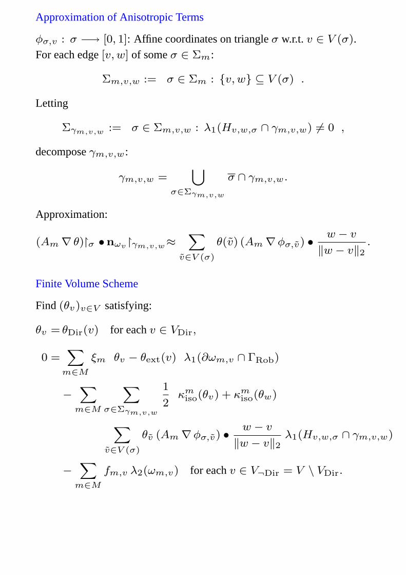
Approximation of Anisotropic Terms

φσ,v : σ −→ [0, 1]: Affine coordinates on triangleσ w.r.t. v ∈ V (σ).For each edge[v, w] of someσ ∈ Σm:

Σm,v,w :=ľσ ∈ Σm : v, w ⊆ V (σ)

ł.

Letting

Σγm,v,w :=ľσ ∈ Σm,v,w : λ1(Hv,w,σ ∩ γm,v,w) 6= 0

ł,

decomposeγm,v,w:

γm,v,w =[

σ∈Σγm,v,w

σ ∩ γm,v,w.

Approximation:

(Am∇ θ)¹σ •nωv¹γm,v,w≈X

v∈V (σ)

θ(v) (Am∇φσ,v) • w − v

‖w − v‖2.

Finite Volume Scheme

Find (θv)v∈V satisfying:

θv = θDir(v) for eachv ∈ VDir,

0 =X

m∈M

ξmąθv − θext(v)

ćλ1(∂ωm,v ∩ ΓRob)

−X

m∈M

X

σ∈Σγm,v,w

1

2

ąκmiso(θv) + κm

iso(θw)ć

X

v∈V (σ)

θv (Am∇φσ,v) • w − v

‖w − v‖2λ1(Hv,w,σ ∩ γm,v,w)

−X

m∈M

fm,v λ2(ωm,v) for eachv ∈ V¬Dir = V \ VDir.

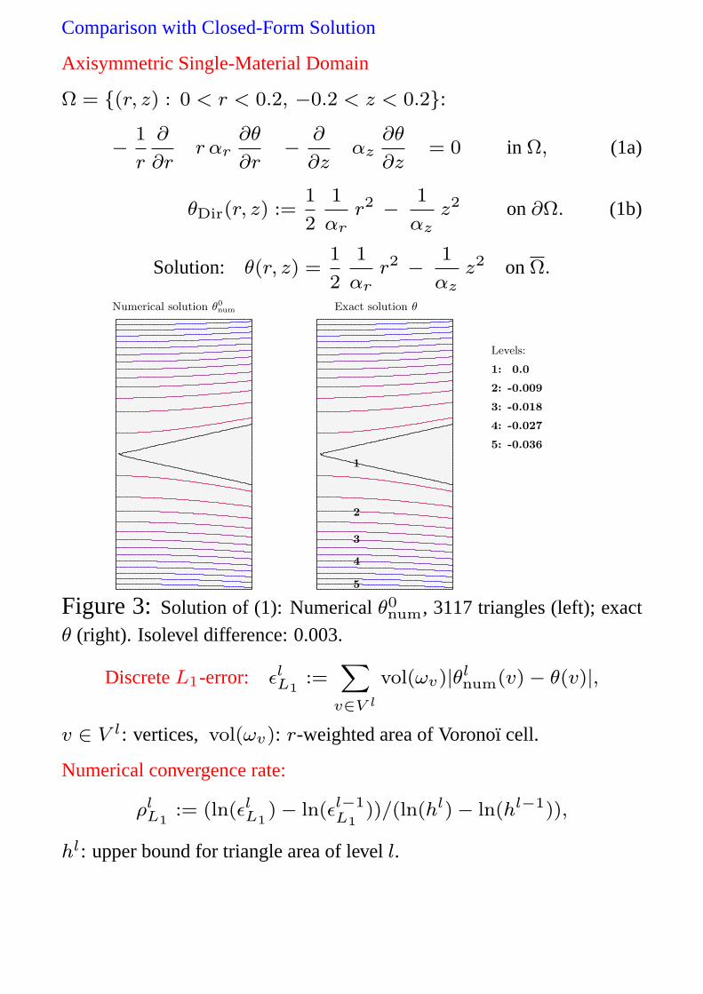
Comparison with Closed-Form Solution

Axisymmetric Single-Material Domain

Ω = (r, z) : 0 < r < 0.2, −0.2 < z < 0.2:

− 1

r

∂

∂r

ţr αr

∂θ

∂r

ű− ∂

∂z

ţαz

∂θ

∂z

ű= 0 in Ω, (1a)

θDir(r, z) :=1

2

1

αrr2 − 1

αzz2 on∂Ω. (1b)

Solution: θ(r, z) =1

2

1

αrr2 − 1

αzz2 onΩ.

Stationary Solution

T_min=-0.04

T_max=0.002

z = 20

z = -20r = 20r = 0

Exact Stationary Solution

T_min=-0.04

T_max=0.002

z = 20

z = -20r = 20r = 0

Numerical solution θ0

num Exact solution θ

Levels:

1: 0.0

2: -0.009

3: -0.018

4: -0.027

5: -0.036

1

2

3

4

5

Figure 3:Solution of (1): Numericalθ0num, 3117 triangles (left); exact

θ (right). Isolevel difference: 0.003.

DiscreteL1-error: εlL1

:=X

v∈V l

vol(ωv)|θlnum(v)− θ(v)|,

v ∈ V l: vertices, vol(ωv): r-weighted area of Voronoı cell.

Numerical convergence rate:

ρlL1

:= (ln(εlL1

)− ln(εl−1L1

))/(ln(hl)− ln(hl−1)),

hl: upper bound for triangle area of levell.

Axisymmetric Multi-Material Domain

Ω1 = (r, z) : 0 < r < r0, 0 < z < z0,Ω2 = (r, z) : r0 < r < rmax, 0 < z < z0,Ω3 = (r, z) : 0 < r < r0, z0 < z < zmax,Ω4 = (r, z) : r0 < r < rmax, z0 < z < zmax,

− 1

r

∂

∂r

ţr αm,r

∂θ

∂r

ű− ∂

∂z

ţαm,z

∂θ

∂z

ű= fm in Ωm, (2a)

0@

0@αm,r 0

0 αm,z

1A∇ θ¹Ωm

1A • nm

=

0@

0@αm,r 0

0 αm,z

1A∇ θ¹Ωm

1A • nm on∂Ωm ∩ ∂Ωm,

(2b)

θDir,m(r, z) := am r2 + bm z2 + cm on∂Ω ∩ ∂Ωm. (2c)

Solution:

θ(r, z) := am r2 + bm z2 + cm onΩm,

θDir,m(r, z) := am r2 + bm z2 + cm on∂Ω ∩ ∂Ωm,

wherer0 = z0 = 0.1, rmax = zmax = 0.2,

α1,r = 2, α2,r = 1, α3,r = 4, α4,r = 2,

α1,z = 1, α2,z = 2, α3,z = 3, α4,z = 6,

a1 = 1, a2 = 2, a3 = 1, a4 = 2,

b1 = 1, b2 = 1, b3 = 1/3, b4 = 1/3,

c1 = 0, c2 = −1/100, c3 = 2/300, c4 = 1/300,

f1 = −10, f2 = −12.0, f3 = −18.0, f4 = −20.0

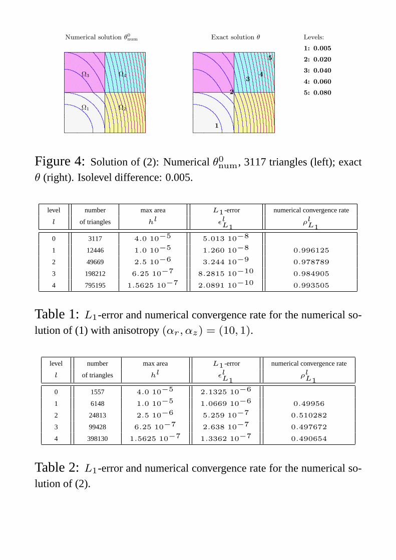
Numerical solution θ0

num Exact solution θ Levels:

1: 0.005

2: 0.020

3: 0.040

4: 0.060

5: 0.080

5

43

2

1

Ω4Ω3

Ω2Ω1

Figure 4:Solution of (2): Numericalθ0num, 3117 triangles (left); exact

θ (right). Isolevel difference: 0.005.

level number max area L1 -error numerical convergence rate

l of triangles hl εlL1

ρlL1

0 3117 4.0 10−5 5.013 10−8

1 12446 1.0 10−5 1.260 10−8 0.996125

2 49669 2.5 10−6 3.244 10−9 0.978789

3 198212 6.25 10−7 8.2815 10−10 0.984905

4 795195 1.5625 10−7 2.0891 10−10 0.993505

Table 1:L1-error and numerical convergence rate for the numerical so-

lution of (1) with anisotropy(αr, αz) = (10, 1).

level number max area L1 -error numerical convergence rate

l of triangles hl εlL1

ρlL1

0 1557 4.0 10−5 2.1325 10−6

1 6148 1.0 10−5 1.0669 10−6 0.49956

2 24813 2.5 10−6 5.259 10−7 0.510282

3 99428 6.25 10−7 2.638 10−7 0.497672

4 398130 1.5625 10−7 1.3362 10−7 0.490654

Table 2:L1-error and numerical convergence rate for the numerical so-

lution of (2).

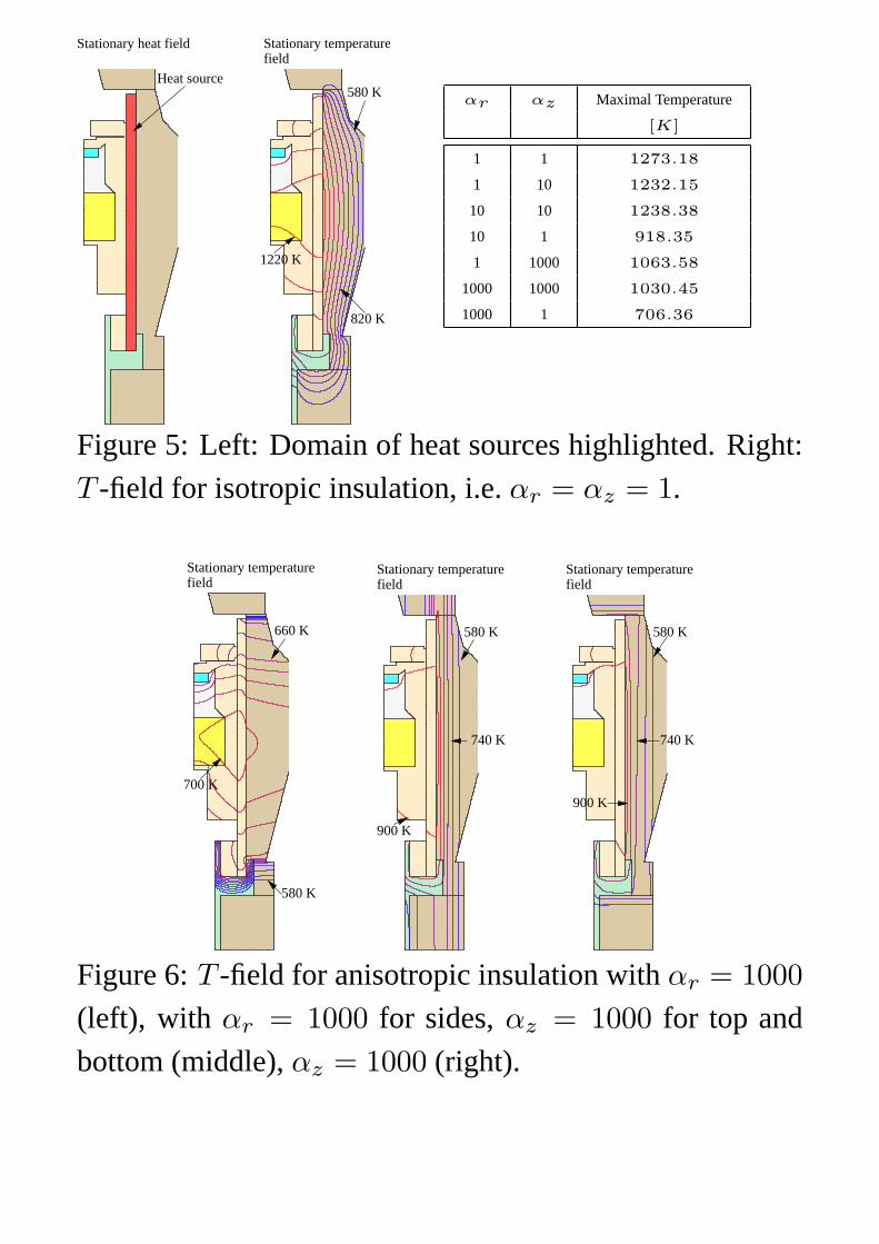
Stationary heat field

Heat source

fieldStationary temperature

1220 K

580 K

820 K

αr αz Maximal Temperature

[K]

1 1 1273.18

1 10 1232.15

10 10 1238.38

10 1 918.35

1 1000 1063.58

1000 1000 1030.45

1000 1 706.36

Figure 5: Left: Domain of heat sources highlighted. Right:

T -field for isotropic insulation, i.e.αr = αz = 1.

fieldStationary temperature

700 K

580 K

660 K

fieldStationary temperature

580 K

740 K

900 K

fieldStationary temperature

580 K

740 K

900 K

Figure 6:T -field for anisotropic insulation withαr = 1000(left), with αr = 1000 for sides,αz = 1000 for top and

bottom (middle),αz = 1000 (right).

Publications

• P. PHILIP : Transient Numerical Simulation of

Sublimation Growth of SiC Bulk Single Crystals.

Modeling, Finite Volume Method, Results,Thesis,

Department of Mathematics, Humboldt University of

Berlin, Germany, 2003 Report No. 22, Weierstrass

Institute for Applied Analysis and Stochastics, Berlin.

• J. GEISER, O. KLEIN , P. PHILIP : Numerical

simulation of heat transfer in materials with

anisotropic thermal conductivity: A finite volume

scheme to handle complex geometries.In preparation.

• J. GEISER, O. KLEIN , P. PHILIP : Influence of

anisotropic thermal conductivity in the apparatus

insulation for sublimation growth of SiC: Numerical

investigation of heat transfer.In preparation.

Funding:

Supported by the DFG Research Center “Matheon:

Mathematics for Key Technologies” in Berlin, by the IMA

in Minneapolis, and by the WIAS in Berlin.