Embed Size (px)
Citation preview
Numerical Methods for Natural Sciences IB Introduction
– 1 –
Numerical MethodsNatural Sciences Tripos 1B
Lecture NotesLent Term 1999
© Stuart DalzielDepartment of Applied Mathematics and Theoretical Physics
University of Cambridge
Phone: (01223) 337911E-mail: [email protected]
WWW: http://www.damtp.cam.ac.uk/user/fdl/people/sd103/Lecture Notes: http://www.damtp.cam.ac.uk/user/fdl/people/sd103/lectures/
Formatting and visibility in this version:
Subsections
Sub-subsections
Fourth order subsectionsAll versions
Full text
Common equations
Handout/lecture equations
Handout/lecture figuresTables
Numerical Methods for Natural Sciences IB Introduction
– 2 –
CONTENTS
• Page numbers are correct only for the hand-out with which they are given
Formatting and visibility in this version: ................................................................................... 1Subsections ................................................................................................................................. 1
Sub-subsections....................................................................................................................... 1
1 Introduction................................................................................................................................ 61.1 Objective............................................................................................................................... 6
1.2 Books .................................................................................................................................... 6General: .................................................................................................................................. 6More specialised:.................................................................................................................... 6
1.3 Programming......................................................................................................................... 7
1.4 Tools ..................................................................................................................................... 71.4.1 Software libraries .......................................................................................................... 71.4.2 Maths systems ................................................................................................................ 7
1.5 Course Credit ........................................................................................................................ 8
1.6 Versions ................................................................................................................................ 81.6.1 Notes disctributed during lectures................................................................................. 81.6.2 Acrobat........................................................................................................................... 81.6.3 HTML............................................................................................................................. 81.6.4 Copyright ....................................................................................................................... 9
2 Key Idea .................................................................................................................................... 10
3 Root finding in one dimension ................................................................................................ 113.1 Why?................................................................................................................................... 11
3.2 Bisection ............................................................................................................................. 113.2.1 Convergence ................................................................................................................ 123.2.2 Criteria......................................................................................................................... 12
3.3 Linear interpolation (regula falsi) ....................................................................................... 13
3.4 Newton-Raphson................................................................................................................. 143.4.1 Convergence ................................................................................................................ 15
3.5 Secant (chord) ..................................................................................................................... 163.5.1 Convergence ................................................................................................................ 18
3.6 Direct iteration .................................................................................................................... 193.6.1 Convergence ................................................................................................................ 20
3.7 Examples............................................................................................................................. 213.7.1 Bisection method.......................................................................................................... 213.7.2 Linear interpolation..................................................................................................... 223.7.3 Newton-Raphson.......................................................................................................... 223.7.4 Secant method .............................................................................................................. 223.7.5 Direct iteration ............................................................................................................ 23
Numerical Methods for Natural Sciences IB Introduction
– 3 –
3.7.6 Comparison.................................................................................................................. 253.7.7 Fortran program* ........................................................................................................ 26
4 Linear equations ...................................................................................................................... 294.1 Gauss elimination ............................................................................................................... 29
4.2 Pivoting............................................................................................................................... 324.2.1 Partial pivoting ............................................................................................................ 334.2.2 Full pivoting................................................................................................................. 34
4.3 LU factorisation .................................................................................................................. 35
4.4 Banded matrices.................................................................................................................. 36
4.5 Tridiagonal matrices ........................................................................................................... 37
4.6 Other approaches to solving linear systems........................................................................ 38
4.7 Over determined systems*................................................................................................... 38
4.8 Under determined systems*................................................................................................. 40
5 Numerical integration.............................................................................................................. 415.1 Manual method ................................................................................................................... 41
5.2 Constant rule ....................................................................................................................... 41
5.3 Trapezium rule.................................................................................................................... 42
5.4 Mid-point rule ..................................................................................................................... 45
5.5 Simpson’s rule .................................................................................................................... 47
5.6 Quadratic triangulation* ...................................................................................................... 48
5.7 Romberg integration ........................................................................................................... 49
5.8 Gauss quadrature................................................................................................................. 50
5.9 Example of numerical integration....................................................................................... 515.9.1 Program for numerical integration* ............................................................................ 54
6 First order ordinary differential equations ........................................................................... 576.1 Taylor series........................................................................................................................ 57
6.2 Finite difference.................................................................................................................. 57
6.3 Truncation error .................................................................................................................. 58
6.4 Euler method....................................................................................................................... 59
6.5 Implicit methods ................................................................................................................. 606.5.1 Backward Euler ........................................................................................................... 606.5.2 Richardson extrapolation ............................................................................................ 626.5.3 Crank-Nicholson.......................................................................................................... 62
6.6 Multistep methods............................................................................................................... 64
6.7 Stability ............................................................................................................................... 64
6.8 Predictor-corrector methods................................................................................................666.8.1 Improved Euler method................................................................................................ 676.8.2 Runge-Kutta methods................................................................................................... 68
7 Higher order ordinary differential equations ....................................................................... 707.1 Initial value problems ......................................................................................................... 70
7.2 Boundary value problems ................................................................................................... 707.2.1 Shooting method .......................................................................................................... 71
Numerical Methods for Natural Sciences IB Introduction
– 4 –
7.2.2 Linear equations .......................................................................................................... 71
7.3 Other considerations* .......................................................................................................... 737.3.1 Truncation error*......................................................................................................... 737.3.2 Error and step control* ................................................................................................ 73
8 Partial differential equations .................................................................................................. 748.1 Laplace equation ................................................................................................................. 74
8.1.1 Direct solution ............................................................................................................. 758.1.2 Relaxation .................................................................................................................... 778.1.3 Multigrid*..................................................................................................................... 818.1.4 The mathematics of relaxation* ................................................................................... 828.1.5 FFT* ............................................................................................................................. 868.1.6 Boundary elements* ..................................................................................................... 868.1.7 Finite elements*............................................................................................................ 86
8.2 Poisson equation ................................................................................................................. 86
8.3 Diffusion equation .............................................................................................................. 868.3.1 Semi-discretisation....................................................................................................... 868.3.2 Euler method................................................................................................................ 878.3.3 Stability ........................................................................................................................ 878.3.4 Model for general initial conditions ............................................................................ 898.3.5 Crank-Nicholson.......................................................................................................... 898.3.6 ADI* ............................................................................................................................. 90
8.4 Advection*........................................................................................................................... 908.4.1 Upwind differencing* ................................................................................................... 908.4.2 Courant number*.......................................................................................................... 908.4.3 Numerical dispersion*.................................................................................................. 908.4.4 Shocks* ......................................................................................................................... 908.4.5 Lax-Wendroff* .............................................................................................................. 908.4.6 Conservative schemes*................................................................................................. 91
9. Number representation* ......................................................................................................... 929.1. Integers* ............................................................................................................................. 92
9.2. Floating point*.................................................................................................................... 93
9.3. Rounding and truncation error*.......................................................................................... 94
9.4. Endians* ............................................................................................................................. 94
10. Computer languages*............................................................................................................ 9610.1. Procedural verses Object Oriented* ................................................................................. 96
10.2. Fortran 90* ....................................................................................................................... 9610.2.1. Procedural oriented*................................................................................................. 9710.2.2. Fortran enhancements*............................................................................................. 97
10.3. C++* ................................................................................................................................. 9810.3.1. C* .............................................................................................................................. 9810.3.2. Object Oriented* ....................................................................................................... 9810.3.3. Weaknesses* .............................................................................................................. 99
10.4. Others*............................................................................................................................ 10010.4.1. Ada*......................................................................................................................... 10010.4.2. Algol* ...................................................................................................................... 100

Numerical Methods for Natural Sciences IB Introduction
– 5 –
10.4.3. Basic* ...................................................................................................................... 10010.4.4. Cobol* ..................................................................................................................... 10110.4.5. Delphi* .................................................................................................................... 10110.4.6. Forth* ...................................................................................................................... 10110.4.7. Lisp* ........................................................................................................................ 10110.4.8. Modula-2* ............................................................................................................... 10110.4.9. Pascal* .................................................................................................................... 10110.4.10. PL/1* ..................................................................................................................... 10210.4.11. PostScript* ............................................................................................................ 10210.4.12. Prolog* .................................................................................................................. 10210.4.13. Smalltalk* .............................................................................................................. 10210.4.14. Visual Basic* ......................................................................................................... 102
Numerical Methods for Natural Sciences IB Introduction
– 6 –
1 Introduction
These lecture notes are written for the Numerical Methods course as part of the Natural SciencesTripos, Part IB. The notes are intended to compliment the material presented in the lectures ratherthan replace them.
1.1 Objective• To give an overview of what can be done
• To give insight into how it can be done
• To give the confidence to tackle numerical solutions
An understanding of how a method works aids in choosing a method. It can also provide anindication of what can and will go wrong, and of the accuracy which may be obtained.
• To gain insight into the underlying physics
• “The aim of this course is to introduce numerical techniques that can be used oncomputers, rather than to provide a detailed treatment of accuracy or stability” –Lecture Schedule.
Unfortunately the course is now examinable and therefore the material must be presented in amanner consistent with this.
1.2 Books
General:• Numerical Recipes - The Art of Scientific Computing, by Press, Flannery, Teukolsky
& Vetterling (CUP)
• Numerical Methods that Work, by Acton (Harper & Row)
• Numerical Analysis, by Burden & Faires (PWS-Kent)
• Applied Numerical Analysis, by Gerald & Wheatley (Addison-Wesley)
• A Simple Introduction to Numerical Analysis, by Harding & Quinney (Institute ofPhysics Publishing)
• Elementary Numerical Analysis, 3rd Edition, by Conte & de Boor (McGraw-Hill)
More specialised:• Numerical Methods for Ordinary Differential Systems, by Lambert (Wiley)
• Numerical Solution of Partial Differential Equations: Finite Difference Methods, bySmith (Oxford University Press)
For many people, Numerical Recipes is the bible for simple numerical techniques. It contains notonly detailed discussion of the algorithms and their use, but also sample source code for each.
Numerical Methods for Natural Sciences IB Introduction
– 7 –
Numerical Recipes is available for three tastes: Fortran, C and Pascal, with the source codeexamples being taylored for each.
1.3 Programming
While a number of programming examples are given during the course, the course andexamination do not require any knowledge of programming. Numerical results are given toillustrate a point and the code used to compute them presented in these notes purely forcompleteness.
1.4 Tools
Unfortunately this course is too short to be able to provide an introduction to the various toolsavailable to assist with the solution of a wide range of mathematical problems. These tools arewidely available on nearly all computer platforms and fall into two general classes:
1.4.1 Software libraries
These are intended to be linked into your own computer program and provide routines forsolving particular classes of problems.
• NAG
• IMFL
• Numerical Recipes
The first two are commercial packages providing object libraries, while the final of these librariesmirrors the content of the Numerical Recipes book and is available as source code.
1.4.2 Maths systems
These provide a shrink-wrapped solution to a broad class of mathematical problems. Typicallythey have easy-to-use interfaces and provide graphical as well as text or numeric output. Keyfeatures include algebraic analytical solution. There is fierce competition between the variousproducts available and, as a result, development continues at a rapid rate.
• Derive
• Maple
• Mathcad
• Mathematica
• Matlab
• Reduce

Numerical Methods for Natural Sciences IB Introduction
– 8 –
1.5 Course Credit
Prior to the 1995-1996 academic year, this course was not examinable. Since then, however,there have been two examination questions each year. Some indication of the type of examquestions may be gained from earlier tripos papers and from the later examples sheets. Note thatthere has, unfortunately, been a tendency to concentrate on the more analysis side of the course inthe examination questions.
Some of the topics covered in these notes are not examinable. This situation is indicated by anasterisk at the end of the section heading.
1.6 Versions
These lecture notes are available in three forms: the lecture notes distributed during lectures, andthe set available in two formats on the web.
1.6.1 Notes disctributed during lectures
The version distributed during lectures includes blanks for you to fill in the missing details. Thesedetails will be given during the lectures themselves.
1.6.2 Acrobat
The lecture notes are also available over the web. This year’s notes will be provided in Acrobatformat (pdf) and may be found athttp://www.damtp.cam.ac.uk/user/fdl/people/sd103/lectures/
These notes contain all the information, and any blanks have been filled in.
1.6.3 HTML
In previous years these have been provided through an html format, and these notes remainavailable, although may not contain the latest revisions. The HTML version of the notes also has allthe blanks filled in.
The HTML is generated from a source Word document that contains graphics, display equationsand inline equations and symbols. All graphics and complex display equations (where the MicrosoftEquation Editor has been used) are converted to GIF files for the HTML version. However, many ofthe simpler equations and most of the inline equations and symbols do not use the Equation Editoras this is very inefficient. As a consequence, they appear as characters rather than GIF files in theHTML document. This has major advantages in terms of document size, but can cause problemswith older World Wide Web browsers.
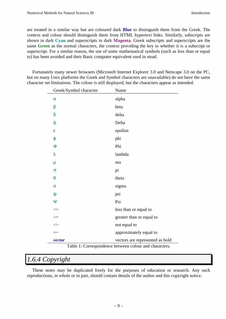
Due to limitations in HTML and many older World Wide Web browsers, Greek and Symbolsused within the text and single line equations may not be displayed correctly. Similarly, somebrowsers do not handle superscript and subscript. To avoid confusion when using older browsers,all Greek and Symbols are formatted in Green. Thus if you find a green Roman character, read it asthe Greek equivalent. Table 1of the correspondences is given below. Variables and normal symbols
Numerical Methods for Natural Sciences IB Introduction
– 9 –
are treated in a similar way but are coloured dark Blue to distinguish them from the Greek. Thecontext and colour should distinguish them from HTML hypertext links. Similarly, subscripts areshown in dark Cyan and superscripts in dark Magenta. Greek subscripts and superscripts are thesame Green as the normal characters, the context providing the key to whether it is a subscript orsuperscript. For a similar reason, the use of some mathematical symbols (such as less than or equalto) has been avoided and their Basic computer equivalent used in stead.
Fortunately many newer browsers (Microsoft Internet Explorer 3.0 and Netscape 3.0 on the PC,but on many Unix platforms the Greek and Symbol characters are unavailable) do not have the samecharacter set limitations. The colour is still displayed, but the characters appear as intended.
Greek/Symbol character Name
α alpha
β beta
δ delta
∆ Delta
ε epsilon
ϕ phi
Φ Phi
λ lambda
µ mu
π pi
θ theta
σ sigma
ψ psi
Ψ Psi
<= less than or equal to
>= greater than or equal to
<> not equal to
=~ approximately equal to
vector vectors are represented as boldTable 1: Correspondence between colour and characters.
1.6.4 Copyright
These notes may be duplicated freely for the purposes of education or research. Any suchreproductions, in whole or in part, should contain details of the author and this copyright notice.
Numerical Methods for Natural Sciences IB Introduction
– 10 –
2 Key Idea
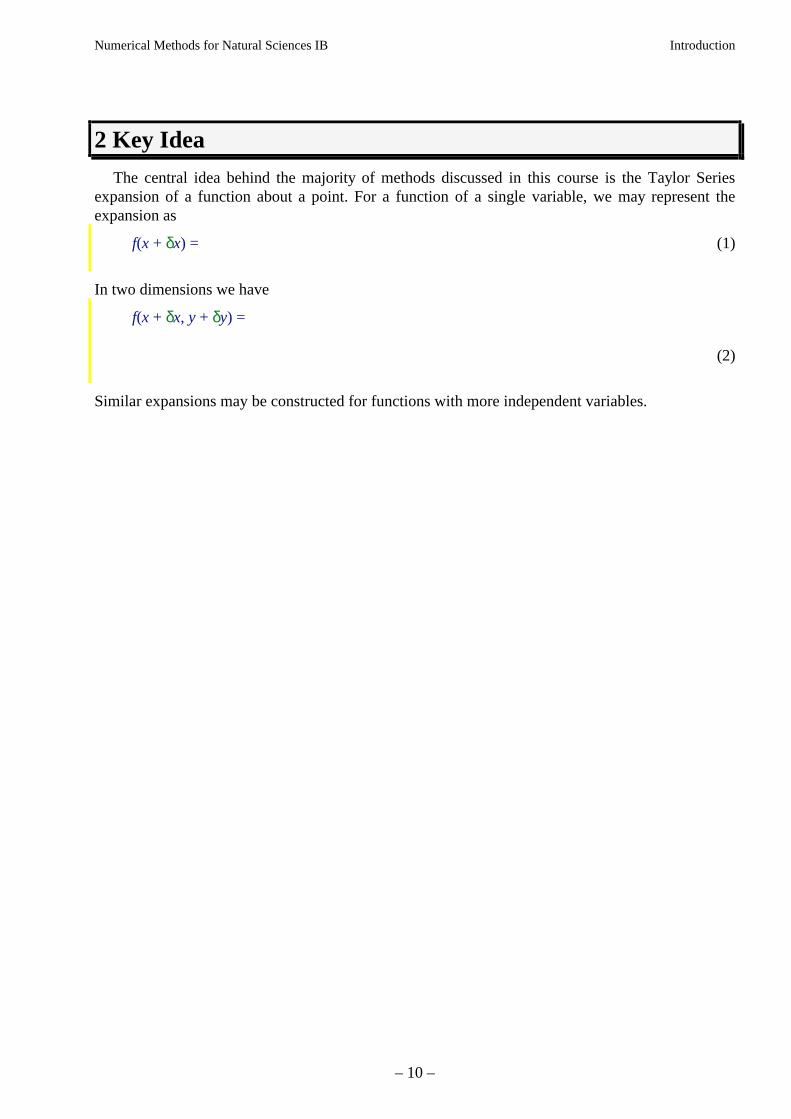
The central idea behind the majority of methods discussed in this course is the Taylor Seriesexpansion of a function about a point. For a function of a single variable, we may represent theexpansion as
f(x + δx) = (1)
In two dimensions we have
f(x + δx, y + δy) =
(2)
Similar expansions may be constructed for functions with more independent variables.
Numerical Methods for Natural Sciences IB Introduction
– 11 –
3 Root finding in one dimension
3.1 Why?
Solutions x = x0 to equations of the form f(x) = 0 are often required where it is impossible orinfeasible to find an analytical expression for the vector x. If the scalar function f depends on mindependent variables x1,x2,…,xm, then the solution x0 will describe a surface in m–1 dimensionalspace. Alternatively we may consider the vector function f(x)=0, the solutions of which typicallycollapse to particular values of x. For this course we restrict our attention to a single independentvariable x and seek solutions to f(x)=0.
3.2 Bisection
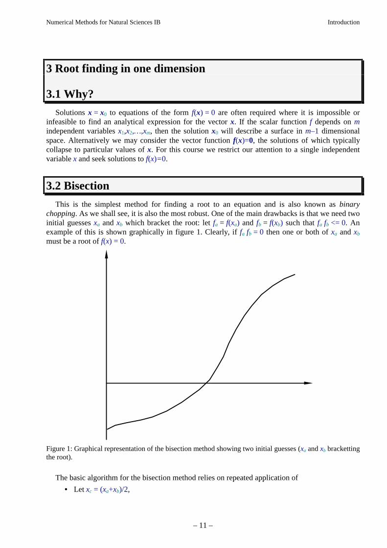
This is the simplest method for finding a root to an equation and is also known as binarychopping. As we shall see, it is also the most robust. One of the main drawbacks is that we need twoinitial guesses xa and xb which bracket the root: let fa = f(xa) and fb = f(xb) such that fa fb <= 0. Anexample of this is shown graphically in figure 1. Clearly, if fa fb = 0 then one or both of xa and xb
must be a root of f(x) = 0.
Figure 1: Graphical representation of the bisection method showing two initial guesses (xa and xb brackettingthe root).
The basic algorithm for the bisection method relies on repeated application of
• Let xc = (xa+xb)/2,
Numerical Methods for Natural Sciences IB Introduction
– 12 –
• if fc = f(c) = 0 then x = xc is an exact solution,
• elseif fa fc < 0 then the root lies in the interval (xa,xc),
• else the root lies in the interval (xc,xb).
By replacing the interval (xa,xb) with either (xa,xc) or (xc,xb) (whichever brackets the root), the errorin our estimate of the solution to f(x) = 0 is, on average, halved. We repeat this interval halvinguntil either the exact root has been found or the interval is smaller than some specified tolerance.
3.2.1 Convergence
Since the interval (xa,xb) always bracets the root, we know that the error in using either xa or xb asan estimate for root at the nth iteration, en, must be
en < |xa - xb|. (3)
Now since the interval (xa,xb) is halved for each iteration, then
en+1 ~ (4)
More generally, if xn is the estimate for the root x* at the nth iteration, then the error in thisestimate is
εn = (5)
In many cases we may express the error at the n+1th time step in terms of the error at the nth timestep as
|εn+1| ~ (6)
Indeed this criteria applies to all techniques discussed in this course, but in many cases it appliesonly asymptotically as our estimate xn converges on the exact solution. The exponent p in equation(6) gives the order of the convergence. The larger the value of p, the faster the scheme converges onthe solution, at least provided εn+1 < εn. For first order schemes (i.e. p = 1), |C| < 1 for convergence.
For the bisection method we may estimate εn as en. The form of equation (4) then suggests p = 1and C = 1/2, showing the scheme is first order and converges linearly. Indeed convergence isguaranteed - a root to f(x) = 0 will always be found - provided f(x) is continuous over the initialinterval.
3.2.2 Criteria
In general, a numerical root finding procedure will not find the exact root being sought (ε = 0),rather it will find some suitably accurate approximation to it. In order to prevent the algorithmcontinuing to refine the solution for ever, it is necessary to place some conditions under which thesolution process is to be finished or aborted. Typically this will take the form of an error toleranceon en = |an–bn|, the value of fc, or both.
For some methods it is also important to ensure the algorithm is converging on a solution (i.e.|εn+1| < |εn| for suitably large n), and that this convergence is sufficiently rapid to attain the solutionin a reasonable span of time. The guaranteed convergence of the bisection method does not require
Numerical Methods for Natural Sciences IB Introduction
– 13 –
such safety checks which, combined with its extreme simplicity, is one of the reasons for itswidespread use despite being relatively slow to converge.
3.3 Linear interpolation (regula falsi)
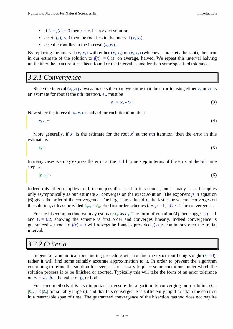
This method is similar to the bisection method in that it requires two initial guesses to bracket theroot. However, instead of simply dividing the region in two, a linear interpolation is used to obtain anew point which is (hopefully, but not necessarily) closer to the root than the equivalent estimate forthe bisection method. A graphical interpretation of this method is shown in figure 2.
xa
xb
Figure 2: Root finding by the linear interpolation (regula falsi) method. The two initial gueses xa and xb mustbracket the root.
The basic algorithm for the linear interpolation method is
• Let x xx x
f ff x
x x
f ff
x f x f
f fc ab a
b aa b
b a
b ab
a b b a
b a
= −−−
= −−−
=−−
, then
• if fc = f(xc) = 0 then x = xc is an exact solution,
• elseif fa fc < 0 then the root lies in the interval (xa,xc),
• else the root lies in the interval (xc,xb).
Because the solution remains bracketed at each step, convergence is guaranteed as was the case forthe bisection method. The method is first order and is exact for linear f.
Numerical Methods for Natural Sciences IB Introduction
– 14 –
3.4 Newton-Raphson
Consider the Taylor Series expansion of f(x) about some point x = x0:
f(x) = (7)
Setting the quadratic and higher terms to zero and solving the linear approximation of f(x) = 0 for xgives
x1 = (8)
Subsequent iterations are defined in a similar manner as
xn+1 = (9)
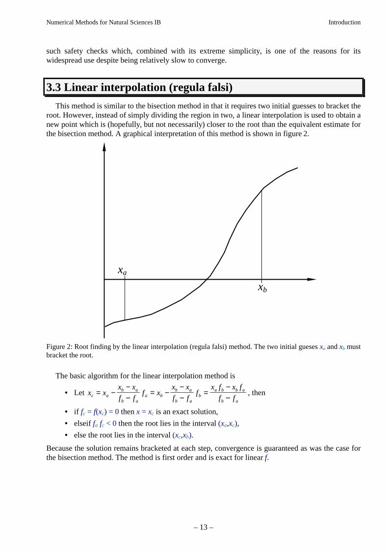
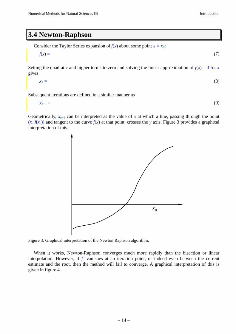
Geometrically, xn+1 can be interpreted as the value of x at which a line, passing through the point(xn,f(xn)) and tangent to the curve f(x) at that point, crosses the y axis. Figure 3 provides a graphicalinterpretation of this.
x0
Figure 3: Graphical interpretation of the Newton Raphson algorithm.
When it works, Newton-Raphson converges much more rapidly than the bisection or linearinterpolation. However, if f’ vanishes at an iteration point, or indeed even between the currentestimate and the root, then the method will fail to converge. A graphical interpretation of this isgiven in figure 4.
Numerical Methods for Natural Sciences IB Introduction
– 15 –
x0
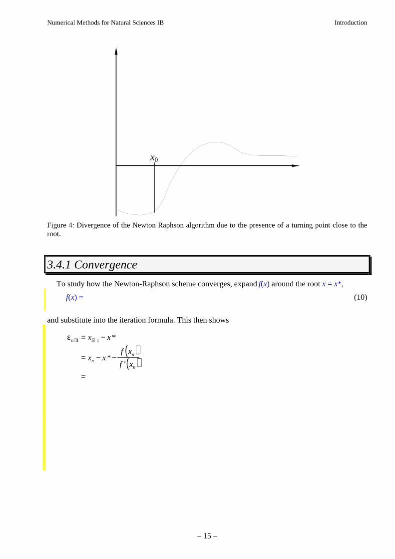
Figure 4: Divergence of the Newton Raphson algorithm due to the presence of a turning point close to theroot.
3.4.1 Convergence
To study how the Newton-Raphson scheme converges, expand f(x) around the root x = x* ,
f(x) = (10)
and substitute into the iteration formula. This then shows
( )( )
εn n
nn
n
x x
x xf x
f x
+ += −
= − −′
=
1 1 *
*
Numerical Methods for Natural Sciences IB Introduction
– 16 –
(11)
since f(x*)=0. Thus, by comparison with (5), there is second order (quadratic) convergence. Thepresence of the f’ term in the denominator shows that the scheme will not converge if f’ vanishes inthe neighbourhood of the root.
3.5 Secant (chord)
This method is essentially the same as Newton-Raphson except that the derivative f’ (x) isapproximated by a finite difference based on the current and the preceding estimate for the root, i.e.
f'(xn) ≈ (12)
and this is substituted into the Newton-Raphson algorithm (9) to give
xn+1 = (13)
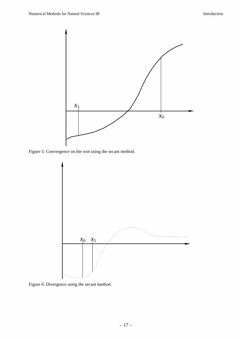
This formula is identical to that for the Linear Interpolation method discussed in section 3.3. Thedifference is that rather than replacing one of the two estimates so that the root is always bracketed,the oldest point is always discarded in favour of the new. This means it is not necessary to have twoinitial guesses bracketing the root, but on the other hand, convergence is not guaranteed. A graphicalrepresentation of the method working is shown in figure 5 and failure to converge in figure 6. Insome cases, swapping the two initial guesses x0 and x1 will change the behaviour of the methodfrom convergent to divergent.
Numerical Methods for Natural Sciences IB Introduction
– 17 –
x1
x0
Figure 5: Convergence on the root using the secant method.
x0 x1
Figure 6: Divergence using the secant method.
Numerical Methods for Natural Sciences IB Introduction
– 18 –
3.5.1 Convergence
The order of convergence may be obtained in a similar way to the earlier methods. Expandingaround the root x = x* for xn and xn+1 gives
f(xn) = (14a)
f(xn-1) = (14b)
and substituting into the iteration formula
( )( ) ( ) ( )
εn n
nn
n nn n
x x
x xf x
f x f xx x
+ +
−−
= −
= − −−
−
=
1 1
11
*
*
(15)
Note that this expression for εn+1 includes both εn and εn–1. In general we would like it in terms of εn
only. The form of this expression suggests a power law relationship. By writing
εn+1 = (16)
and substituting into the error evolution equation (15) gives
( )( )ε ε εn n n
f x
f x+ −=′′′
=
1 12
*
*
Numerical Methods for Natural Sciences IB Introduction
– 19 –
(17)
which we equate with our assumed relationship to show
αα
α
βα
α
=+
=
=+
=
1
1
(18)
Thus the method is of non-integer order 1.61803… (the golden ratio). As with Newton-Raphson,the method may diverge if f’ vanishes in the neighbourhood of the root.
3.6 Direct iteration
A simple and often useful method involves rearranging and possibly transforming the functionf(x) by T(f(x),x) to obtain g(x) = T(f(x),x). The only restriction on T(f(x),x) is that solutions to f(x) = 0have a one to one relationship with solutions to g(x) = x for the roots being sort. Indeed, one reasonfor choosing such a transformation for an equation with multiple roots is to eliminate known rootsand thus simplify the location of the remaining roots. The efficiency and convergence of thismethod depends on the final form of g(x).
The iteration formula for this method is then just
xn+1 = (19)
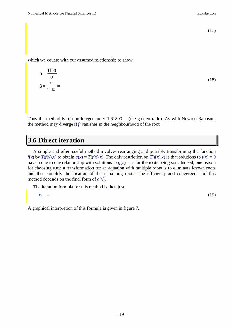
A graphical interpretion of this formula is given in figure 7.
Numerical Methods for Natural Sciences IB Introduction
– 20 –
x0
Figure 7: Convergence on a root using the Direct Iteration method.
3.6.1 Convergence
The convergence of this method may be determined in a similar manner to the other methods byexpanding about x*. Here we need to expand g(x) rather than f(x). This gives
g(xn) = (20)
so that the evolution of the error follows
εn+1 = xn+1 − x
(21)
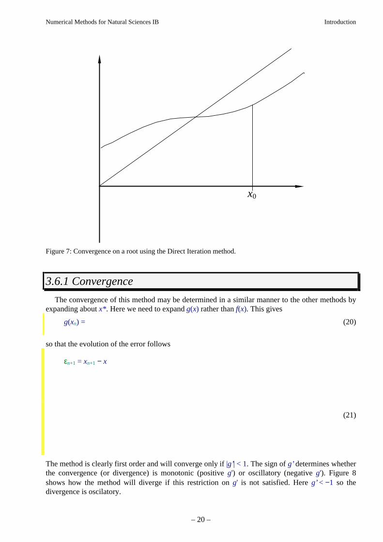
The method is clearly first order and will converge only if |g’| < 1. The sign of g’ determines whetherthe convergence (or divergence) is monotonic (positive g') or oscillatory (negative g'). Figure 8shows how the method will diverge if this restriction on g' is not satisfied. Here g’ < −1 so thedivergence is oscilatory.
Numerical Methods for Natural Sciences IB Introduction
– 21 –
Obviously our choice of T(f(x),x) should try to minimise g’(x) in the neighbourhood of the root tomaximise the rate of convergence. In addition, we should choose T(f(x),x) so that the curvature|g"(x)| does not become too large.
If g’(x) < 0, then we get oscillatory convergence/divergence.
x0
Figure 8: The divergence of a Direct Iteration when g’ < −1.
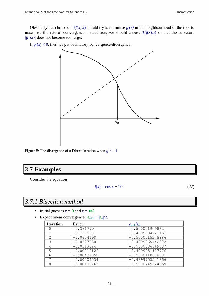
3.7 Examples
Consider the equation
f(x) = cos x − 1/2. (22)
3.7.1 Bisection method• Initial guesses x = 0 and x = π/2.• Expect linear convergence: |εn+1| ~ |εn|/2.
Iteration Error en+1/en0 -0.261799 -0.5000019098621 0.130900 -0.49999847211612 -0.0654498 -0.50000152788863 0.0327250 -0.49999694423224 -0.0163624 -0.50000366694375 0.00818126 -0.49999511077766 -0.00409059 -0.50001100085817 0.00204534 -0.49997555418668 -0.00102262 -0.5000449824959
Numerical Methods for Natural Sciences IB Introduction
– 22 –
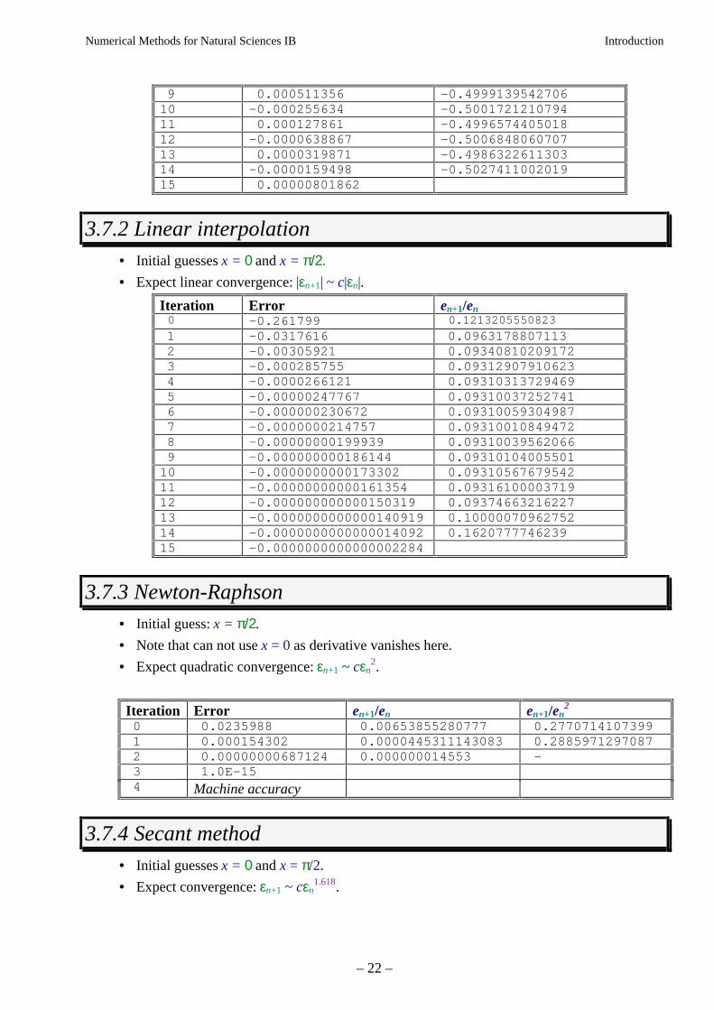
9 0.000511356 -0.499913954270610 -0.000255634 -0.500172121079411 0.000127861 -0.499657440501812 -0.0000638867 -0.500684806070713 0.0000319871 -0.498632261130314 -0.0000159498 -0.502741100201915 0.00000801862
3.7.2 Linear interpolation• Initial guesses x = 0 and x = π/2.• Expect linear convergence: |εn+1| ~ c|εn|.
Iteration Error en+1/en0 -0.261799 0.1213205550823
1 -0.0317616 0.09631788071132 -0.00305921 0.093408102091723 -0.000285755 0.093129079106234 -0.0000266121 0.093103137294695 -0.00000247767 0.093100372527416 -0.000000230672 0.093100593049877 -0.0000000214757 0.093100108494728 -0.00000000199939 0.093100395620669 -0.000000000186144 0.0931010400550110 -0.0000000000173302 0.0931056767954211 -0.00000000000161354 0.0931610000371912 -0.000000000000150319 0.0937466321622713 -0.0000000000000140919 0.1000007096275214 -0.0000000000000014092 0.162077774623915 -0.0000000000000002284
3.7.3 Newton-Raphson• Initial guess: x = π/2.
• Note that can not use x = 0 as derivative vanishes here.
• Expect quadratic convergence: εn+1 ~ cεn2.
Iteration Error en+1/en en+1/en2
0 0.0235988 0.00653855280777 0.27707141073991 0.000154302 0.0000445311143083 0.28859712970872 0.00000000687124 0.000000014553 -3 1.0E-154 Machine accuracy
3.7.4 Secant method• Initial guesses x = 0 and x = π/2.
• Expect convergence: εn+1 ~ cεn1.618.
Numerical Methods for Natural Sciences IB Introduction
– 23 –
Iteration Error en+1/en |en+1|/|en|1.618
0 -0.261799 0.1213205550823 0.27771 -0.0317616 -0.09730712558561 0.82032 0.00309063 -0.009399086917554 0.33443 -0.0000290491 0.0008898244696049 0.56644 -0.0000000258486 -0.000008384051747483 0.40985 0.0000000000002167166 Machine accuracy
• Convergence substantially faster than linear interpolation.
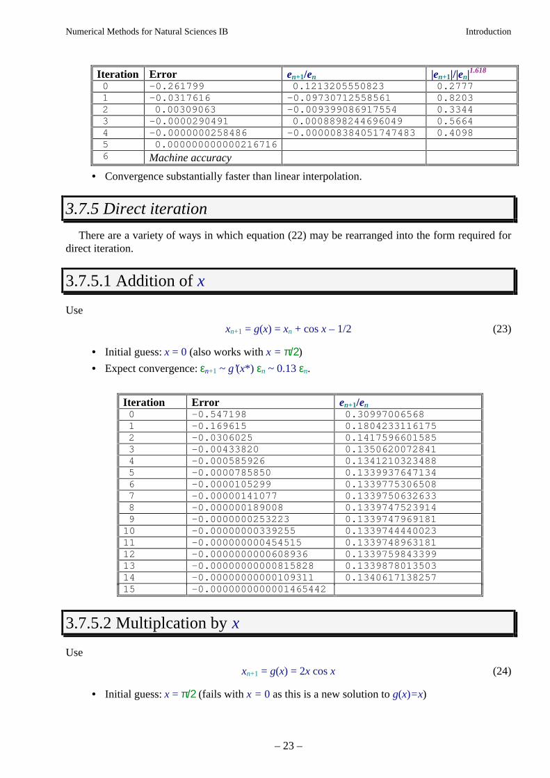
3.7.5 Direct iteration
There are a variety of ways in which equation (22) may be rearranged into the form required fordirect iteration.
3.7.5.1 Addition of x
Use
xn+1 = g(x) = xn + cos x – 1/2 (23)
• Initial guess: x = 0 (also works with x = π/2)
• Expect convergence: εn+1 ~ g’(x*) εn ~ 0.13 εn.
Iteration Error en+1/en0 -0.547198 0.309970065681 -0.169615 0.18042331161752 -0.0306025 0.14175966015853 -0.00433820 0.13506200728414 -0.000585926 0.13412103234885 -0.0000785850 0.13399376471346 -0.0000105299 0.13397753065087 -0.00000141077 0.13397506326338 -0.000000189008 0.13397475239149 -0.0000000253223 0.133974796918110 -0.00000000339255 0.133974444002311 -0.000000000454515 0.133974896318112 -0.0000000000608936 0.133975984339913 -0.00000000000815828 0.133987801350314 -0.00000000000109311 0.134061713825715 -0.0000000000001465442
3.7.5.2 Multiplcation by x
Use
xn+1 = g(x) = 2x cos x (24)
• Initial guess: x = π/2 (fails with x = 0 as this is a new solution to g(x)=x)
Numerical Methods for Natural Sciences IB Introduction
– 24 –
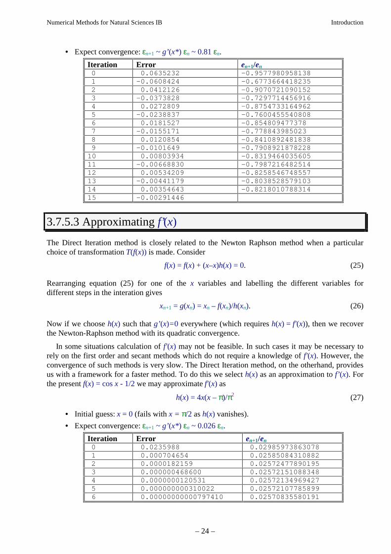
• Expect convergence: εn+1 ~ g’(x*) εn ~ 0.81 εn.
Iteration Error en+1/en0 0.0635232 -0.95779809581381 -0.0608424 -0.67736644182352 0.0412126 -0.90707210901523 -0.0373828 -0.72977144569164 0.0272809 -0.87547331649625 -0.0238837 -0.76004555408086 0.0181527 -0.8548094773787 -0.0155171 -0.7788439850238 0.0120854 -0.84108924818389 -0.0101649 -0.790892187822810 0.00803934 -0.831946403560511 -0.00668830 -0.798721648251412 0.00534209 -0.825854674855713 -0.00441179 -0.803852857910314 0.00354643 -0.821801078831415 -0.00291446
3.7.5.3 Approximating f’(x)
The Direct Iteration method is closely related to the Newton Raphson method when a particularchoice of transformation T(f(x)) is made. Consider
f(x) = f(x) + (x–x)h(x) = 0. (25)
Rearranging equation (25) for one of the x variables and labelling the different variables fordifferent steps in the interation gives
xn+1 = g(xn) = xn – f(xn)/h(xn). (26)
Now if we choose h(x) such that g’(x)=0 everywhere (which requires h(x) = f'(x)), then we recoverthe Newton-Raphson method with its quadratic convergence.
In some situations calculation of f'(x) may not be feasible. In such cases it may be necessary torely on the first order and secant methods which do not require a knowledge of f'(x). However, theconvergence of such methods is very slow. The Direct Iteration method, on the otherhand, providesus with a framework for a faster method. To do this we select h(x) as an approximation to f’ (x). Forthe present f(x) = cos x - 1/2 we may approximate f'(x) as
h(x) = 4x(x – π)/π2 (27)
• Initial guess: x = 0 (fails with x = π/2 as h(x) vanishes).
• Expect convergence: εn+1 ~ g’(x*) εn ~ 0.026 εn.
Iteration Error en+1/en0 0.0235988 0.029859738630781 0.000704654 0.025850843108822 0.0000182159 0.025724778901953 0.000000468600 0.025721510883484 0.0000000120531 0.025721349694275 0.000000000310022 0.025721077858996 0.00000000000797410 0.02570835580191
Numerical Methods for Natural Sciences IB Introduction
– 25 –
7 0.000000000000205001 0.025212072136238 0.000000000000005168509 Machine accuracy
The convergence, while still formally linear, is significantly more rapid than with the other firstorder methods. For a more complex example, the computational cost of having more iterations thanNewton Raphson may be significantly less than the cost of evaluating the derivative.
A further potential use of this approach is to avoid the divergence problems associated with f’(x)vanishing in the Newton Raphson scheme. Since h(x) only approximates f’(x), and the accuracy ofthis approximation is more important close to the root, it may be possible to choose h(x) in such away as to avoid a divergent scheme.
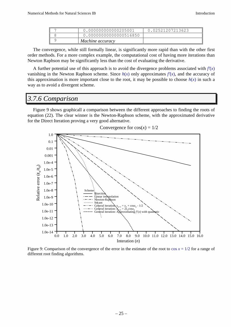
3.7.6 Comparison
Figure 9 shows graphicall a comparison between the different approaches to finding the roots ofequation (22). The clear winner is the Newton-Raphson scheme, with the approximated derivativefor the Direct Iteration proving a very good alternative.
0.0 1.0 2.0 3.0 4.0 5.0 6.0 7.0 8.0 9.0 10.0 11.0 12.0 13.0 14.0 15.0 16.01.0e-14
1.0e-13
1.0e-12
1.0e-11
1.0e-10
1.0e-9
1.0e-8
1.0e-7
1.0e-6
1.0e-5
1.0e-4
0.001
0.01
0.1
1.0
Interation (n)
Rel
ativ
e er
ror
(εn/
ε 0)
Convergence for cos(x) = 1/2
Scheme Bisection Linear interpolation Newton-Raphson Secant General iteration: xn+1 = xn + cosxn - 1/2 General iteration: xn+1 = 2xncosxn General iteration: Approximating f’(x) with quadratic
Figure 9: Comparison of the convergence of the error in the estimate of the root to cos x = 1/2 for a range ofdifferent root finding algorithms.

Numerical Methods for Natural Sciences IB Introduction
– 26 –
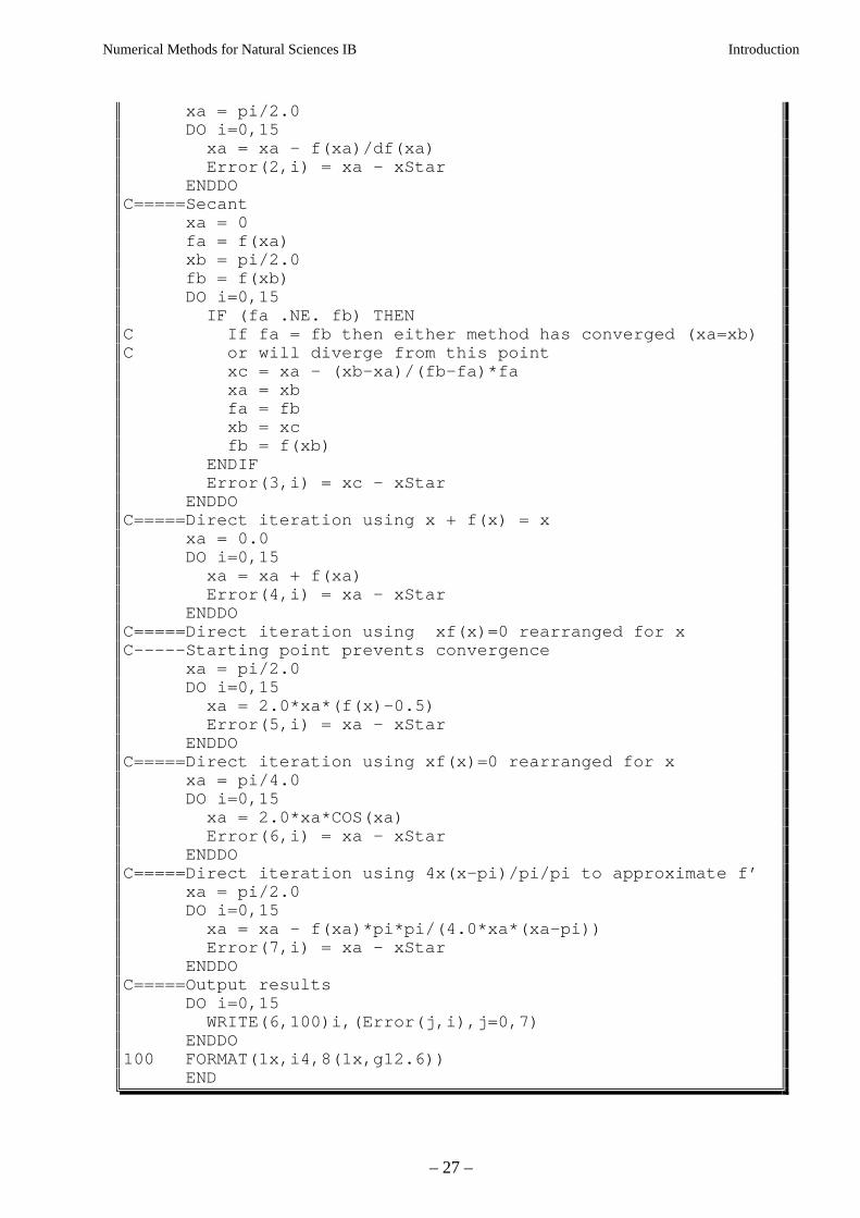
3.7.7 Fortran program*
The following program was used to generate the data presented for the above examples. Notethat this is included as an illustrative example. No knowledge of Fortran or any other programminglanguage is required in this course.
PROGRAM Roots INTEGER*4 i,j REAL*8 x,xa,xb,xc,fa,fb,fc,pi,xStar,f,df REAL*8 Error(0:15,0:15) f(x)=cos(x)-0.5 df(x) = -SIN(x) pi = 3.141592653 xStar = ACOS(0.5) WRITE(6,*)’# ’,xStar,f(xStar)C=====Bisection xa = 0 fa = f(xa) xb = pi/2.0 fb = f(xb) DO i=0,15 xc = (xa + xb)/2.0 fc = f(xc) IF (fa*fc .LT. 0.0) THEN xb = xc fb = fc ELSE xa = xc fa = fc ENDIF Error(0,i) = xc - xStar ENDDOC=====Linear interpolation xa = 0 fa = f(xa) xb = pi/2.0 fb = f(xb) DO i=0,15 xc = xa - (xb-xa)/(fb-fa)*fa fc = f(xc) IF (fa*fc .LT. 0.0) THEN xb = xc fb = fc ELSE xa = xc fa = fc ENDIF Error(1,i) = xc - xStar ENDDOC=====Newton-Raphson
* Not examinable
Numerical Methods for Natural Sciences IB Introduction
– 27 –
xa = pi/2.0 DO i=0,15 xa = xa - f(xa)/df(xa) Error(2,i) = xa - xStar ENDDOC=====Secant xa = 0 fa = f(xa) xb = pi/2.0 fb = f(xb) DO i=0,15 IF (fa .NE. fb) THENC If fa = fb then either method has converged (xa=xb)C or will diverge from this point xc = xa - (xb-xa)/(fb-fa)*fa xa = xb fa = fb xb = xc fb = f(xb) ENDIF Error(3,i) = xc - xStar ENDDOC=====Direct iteration using x + f(x) = x xa = 0.0 DO i=0,15 xa = xa + f(xa) Error(4,i) = xa - xStar ENDDOC=====Direct iteration using xf(x)=0 rearranged for xC-----Starting point prevents convergence xa = pi/2.0 DO i=0,15 xa = 2.0*xa*(f(x)-0.5) Error(5,i) = xa - xStar ENDDOC=====Direct iteration using xf(x)=0 rearranged for x xa = pi/4.0 DO i=0,15 xa = 2.0*xa*COS(xa) Error(6,i) = xa - xStar ENDDOC=====Direct iteration using 4x(x-pi)/pi/pi to approximate f’ xa = pi/2.0 DO i=0,15 xa = xa - f(xa)*pi*pi/(4.0*xa*(xa-pi)) Error(7,i) = xa - xStar ENDDOC=====Output results DO i=0,15 WRITE(6,100)i,(Error(j,i),j=0,7) ENDDO100 FORMAT(1x,i4,8(1x,g12.6)) END

Numerical Methods for Natural Sciences IB Introduction
– 28 –

Numerical Methods for Natural Sciences IB Introduction
– 29 –
4 Linear equations
Solving equation of the form Ax = r is central to many numerical algorithms. There are a numberof methods which may be used, some algebraically correct, while others iterative in nature andproviding only approximate solutions. Which is best will depend on the structure of A, the contextin which it is to be solved and the size compared with the available computer resources.
4.1 Gauss elimination
This is what you would probably do if you were computing the solution of a non-trivial systemby hand. For example, if
x y z
x y z
x y z
+ + =+ + =+ + =
2 3 6
2 2 3 7
4 4 9
, (28)
we might then subtract 2 times the first equation from the second equation, and subtract the firstequation from the third equation to get
(29)
In the second step we might add the second equation to the third to obtain
(30)
The third equation now involves only z giving z = 1. Substituting this back into the second equationgives an equation for y and so-on. In particular we have
(31)
Numerical Methods for Natural Sciences IB Introduction
– 30 –
We may write this system in terms of a matrix A, an unknown vector x and the known right-handside b as
(32)
and do exactly the same manipulations on the rows of the matrix A and right-hand side b. From thesystem
(33)
we subract 2 times the first row from the second row, and subtract the first row from the third rowto obtain
(34)
Before adding the second and third rows, this time we will divide the second row through by −2, theelement on the diagonal, getting
(35)
This may seem pointless in this example, but in general it simplifies the next step where we subtracta32 times the second row from the third row. Here a32 = 2 and represents the value in the secondcolumn of the third row of the matrix. Thus the next step is
(36)
(37)
We again divide the resulting row (now the third row) by the element on the diagonal (a33 = −2) toobtain
(38)
Numerical Methods for Natural Sciences IB Introduction
– 31 –
and retrieve immediately the value z = 1 from the last row of the equation. Substituting back we get
(39)
and finally we recover the answer
(40)
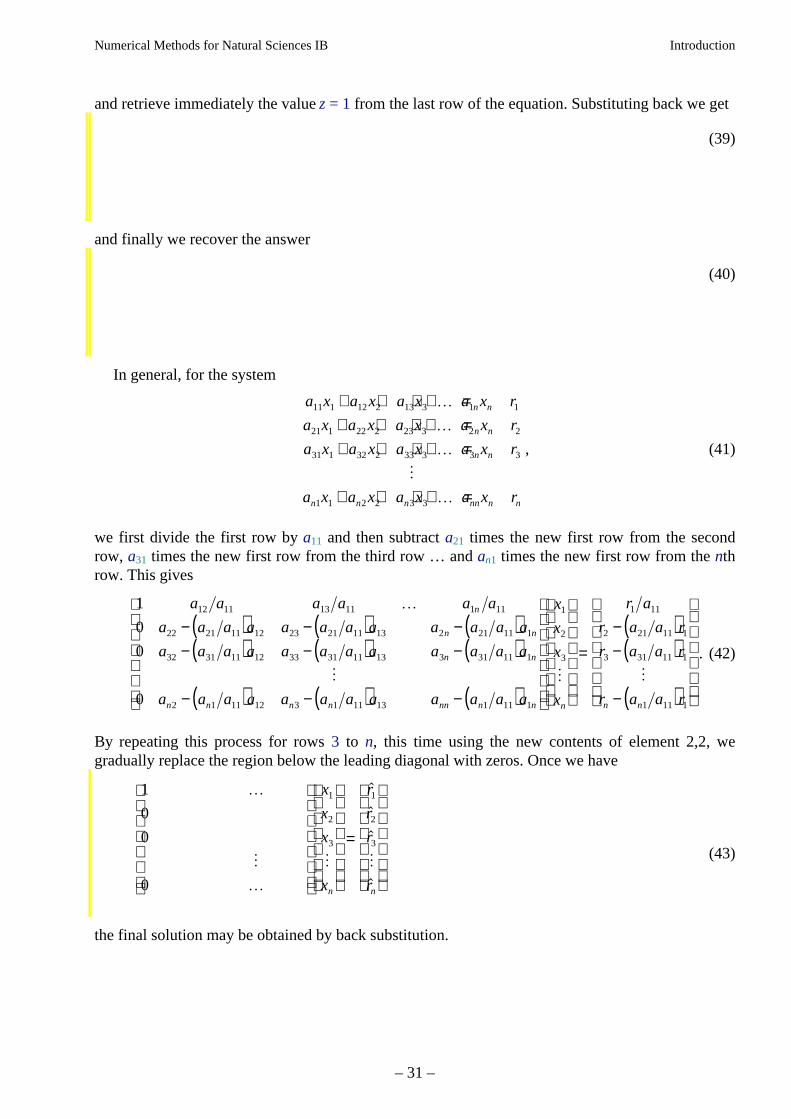
In general, for the system
a x a x a x a x r
a x a x a x a x r
a x a x a x a x r
a x a x a x a x r
n n
n n
n n
n n n nn n n
11 1 12 2 13 3 1 1
21 1 22 2 23 3 2 2
31 1 32 2 33 3 3 3
1 1 2 2 3 3
+ + + + =+ + + + =+ + + + =
+ + + + =
K
K
K
M
K
, (41)
we first divide the first row by a11 and then subtract a21 times the new first row from the secondrow, a31 times the new first row from the third row … and an1 times the new first row from the nthrow. This gives
( ) ( ) ( )( ) ( ) ( )
( ) ( ) ( )
1
0
0
0
12 11 13 11 1 11
22 21 11 12 23 21 11 13 2 21 11 1
32 31 11 12 33 31 11 13 3 31 11 1
2 1 11 12 3 1 11 13 1 11 1
1
2
3
a a a a a a
a a a a a a a a a a a a
a a a a a a a a a a a a
a a a a a a a a a a a a
x
x
x
x
n
n n
n n
n n n n nn n n n
K
M M
− − −− − −
− − −
( )( )
( )
=
−−
−
r a
r a a r
r a a r
r a a rn n
1 11
2 21 11 1
3 31 11 1
1 11 1
M
. (42)
By repeating this process for rows 3 to n, this time using the new contents of element 2,2, wegradually replace the region below the leading diagonal with zeros. Once we have
1
0
0
0
1
2
3
1
2
3
K
M
K
M M
=
x
x
x
x
r
r
r
rn n
$
$
$
$
(43)
the final solution may be obtained by back substitution.
Numerical Methods for Natural Sciences IB Introduction
– 32 –
x
x
x
x
n
n
n
===
=
−
−
1
2
1
M(44)
If the arithmetic is exact, and the matrix A is not singular, then the answer computed in thismanner will be exact (provided no zeros appear on the diagonal - see below). However, as computerarithmetic is not exact, there will be some truncation and rounding error in the answer. Thecumulative effect of this error may be very significant if the loss of precision is at an early stage inthe computation. In particular, if a numerically small number appears on the diagonal of the row,then its use in the elimination of subsequent rows may lead to differences being computed betweenvery large and very small values with a consequential loss of precision. For example, if a22–(a21/a11)a12 were very small, 10–6, say, and both a23–(a21/a11)a13 and a33–(a31/a11)a13 were 1, say,then at the next stage of the computation the 3,3 element would involve calculating the differencebetween 1/10–6=106 and 1. If single precision arithmetic (representing real values usingapproximately six significant digits) were being used, the result would be simply 1.0 and subsequentcalculations would be unaware of the contribution of a23 to the solution. A more extreme case whichmay often occur is if, for example, a22–(a21/a11)a12 is zero – unless something is done it will not bepossible to proceed with the computation!
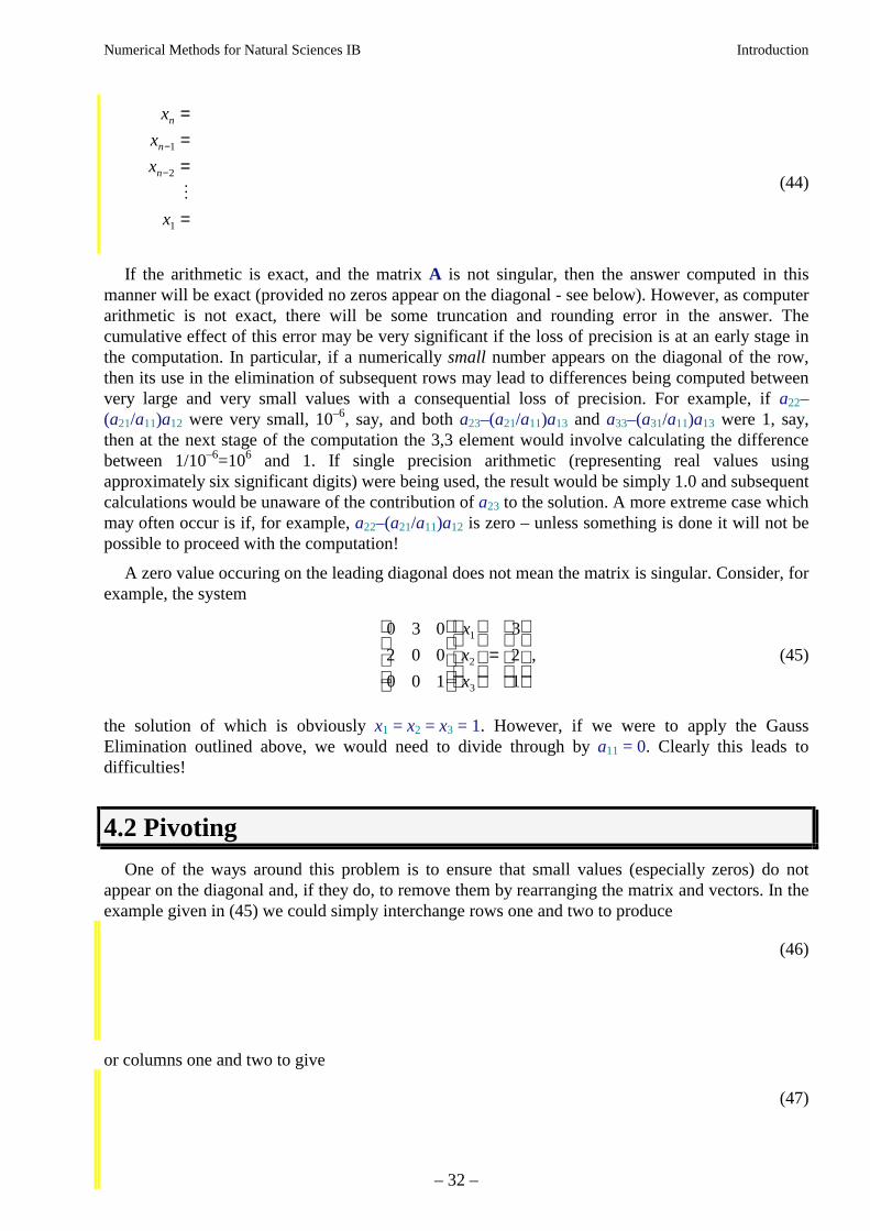
A zero value occuring on the leading diagonal does not mean the matrix is singular. Consider, forexample, the system
0 3 0
2 0 0
0 0 1
3
2
1
1
2
3
=
x
x
x
, (45)
the solution of which is obviously x1 = x2 = x3 = 1. However, if we were to apply the GaussElimination outlined above, we would need to divide through by a11 = 0. Clearly this leads todifficulties!
4.2 Pivoting
One of the ways around this problem is to ensure that small values (especially zeros) do notappear on the diagonal and, if they do, to remove them by rearranging the matrix and vectors. In theexample given in (45) we could simply interchange rows one and two to produce
(46)
or columns one and two to give
(47)
Numerical Methods for Natural Sciences IB Introduction
– 33 –
either of which may then be solved using standard Guass Elimination.
More generally, suppose at some stage during a calculation we have
1 4 1 8 3 2 5
0 10 1 10 201 13 4
0 9 4 6 8 2 18
0 3 2 3 4 6003 15
0 15 1 9 33 2 1
0 155 23 4 25 73 2
0 8 56 4 4 4 88
61
2
3
4
5
6
1
2
3
4
5
6
K
M
K
M M
−
−−
−−
−
=
x
x
x
x
x
x
x
r
r
r
r
r
r
rn n
$
$
$
$
$
$
$
(48)
where the element 2,5 (201) is numerically the largest value in the second row and the element 6,2(155) the numerically largest value in the second column. As discussed above, the very small 10–6
value for element 2,2 is likely to cause problems. (In an extreme case we might even have the value0 appearing on the diagonal – clearly something must be done to avoid a divide by zero erroroccurring!) To remove this problem we may again rearrange the rows and/or columns to bring alarger value into the 2,2 element.
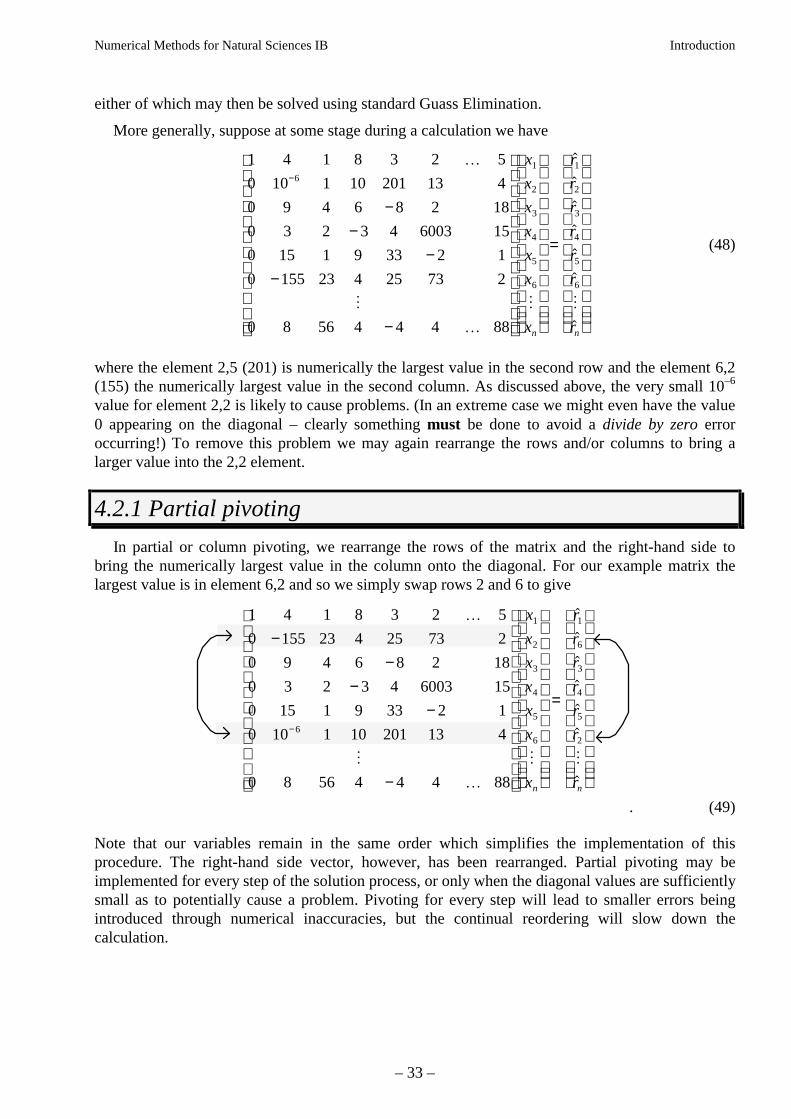
4.2.1 Partial pivoting
In partial or column pivoting, we rearrange the rows of the matrix and the right-hand side tobring the numerically largest value in the column onto the diagonal. For our example matrix thelargest value is in element 6,2 and so we simply swap rows 2 and 6 to give
1 4 1 8 3 2 5
0 155 23 4 25 73 2
0 9 4 6 8 2 18
0 3 2 3 4 6003 15
0 15 1 9 33 2 1
0 10 1 10 201 13 4
0 8 56 4 4 4 88
6
1
2
3
4
5
6
1
6
3
4
5
2
K
M
K
M M
−−
−−
−
=
−
x
x
x
x
x
x
x
r
r
r
r
r
r
rn n
$
$
$
$
$
$
$
. (49)
Note that our variables remain in the same order which simplifies the implementation of thisprocedure. The right-hand side vector, however, has been rearranged. Partial pivoting may beimplemented for every step of the solution process, or only when the diagonal values are sufficientlysmall as to potentially cause a problem. Pivoting for every step will lead to smaller errors beingintroduced through numerical inaccuracies, but the continual reordering will slow down thecalculation.
Numerical Methods for Natural Sciences IB Introduction
– 34 –
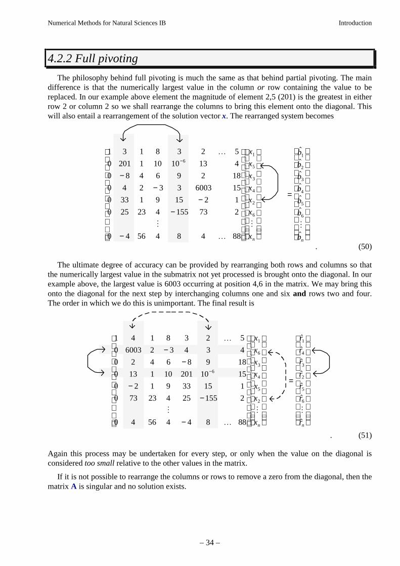
4.2.2 Full pivoting
The philosophy behind full pivoting is much the same as that behind partial pivoting. The maindifference is that the numerically largest value in the column or row containing the value to bereplaced. In our example above element the magnitude of element 2,5 (201) is the greatest in eitherrow 2 or column 2 so we shall rearrange the columns to bring this element onto the diagonal. Thiswill also entail a rearrangement of the solution vector x. The rearranged system becomes
1 3 1 8 3 2 5
0 201 1 10 10 13 4
0 8 4 6 9 2 18
0 4 2 3 3 6003 15
0 33 1 9 15 2 1
0 25 23 4 155 73 2
0 4 56 4 8 4 88
61
5
3
4
2
6
1
2
3
4
5
6
K
M
K
M M
−
−−
−−
−
=
x
x
x
x
x
x
x
b
b
b
b
b
b
bn n
$
$
$
$
$
$
$
. (50)
The ultimate degree of accuracy can be provided by rearranging both rows and columns so thatthe numerically largest value in the submatrix not yet processed is brought onto the diagonal. In ourexample above, the largest value is 6003 occurring at position 4,6 in the matrix. We may bring thisonto the diagonal for the next step by interchanging columns one and six and rows two and four.The order in which we do this is unimportant. The final result is
1 4 1 8 3 2 5
0 6003 2 3 4 3 4
0 2 4 6 8 9 18
0 13 1 10 201 10 15
0 2 1 9 33 15 1
0 73 23 4 25 155 2
0 4 56 4 4 8 88
6
1
6
3
4
5
2
1
4
3
2
5
6
K
M
K
M M
−−
−−
−
=
−
x
x
x
x
x
x
x
r
r
r
r
r
r
rn n
$
$
$
$
$
$
$
. (51)
Again this process may be undertaken for every step, or only when the value on the diagonal isconsidered too small relative to the other values in the matrix.
If it is not possible to rearrange the columns or rows to remove a zero from the diagonal, then thematrix A is singular and no solution exists.
Numerical Methods for Natural Sciences IB Introduction
– 35 –
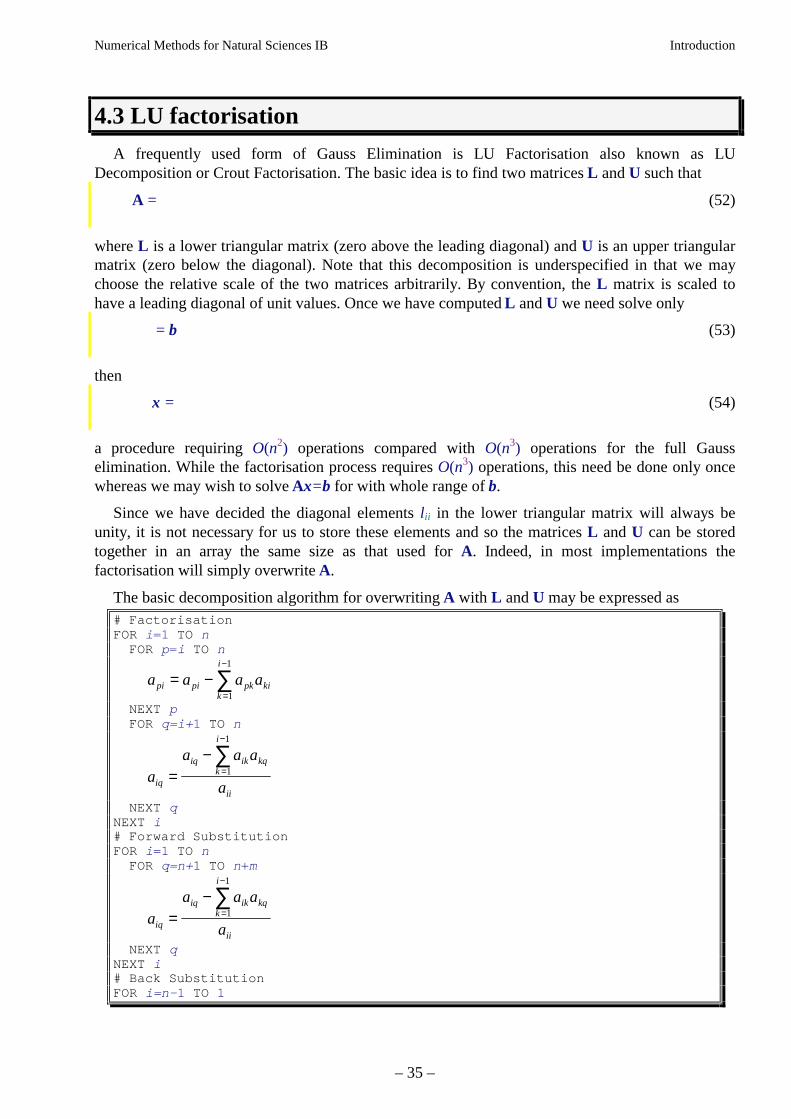
4.3 LU factorisation
A frequently used form of Gauss Elimination is LU Factorisation also known as LUDecomposition or Crout Factorisation. The basic idea is to find two matrices L and U such that
A = (52)
where L is a lower triangular matrix (zero above the leading diagonal) and U is an upper triangularmatrix (zero below the diagonal). Note that this decomposition is underspecified in that we maychoose the relative scale of the two matrices arbitrarily. By convention, the L matrix is scaled tohave a leading diagonal of unit values. Once we have computed L and U we need solve only
= b (53)
then
x = (54)
a procedure requiring O(n2) operations compared with O(n3) operations for the full Gausselimination. While the factorisation process requires O(n3) operations, this need be done only oncewhereas we may wish to solve Ax=b for with whole range of b.
Since we have decided the diagonal elements lii in the lower triangular matrix will always beunity, it is not necessary for us to store these elements and so the matrices L and U can be storedtogether in an array the same size as that used for A. Indeed, in most implementations thefactorisation will simply overwrite A.
The basic decomposition algorithm for overwriting A with L and U may be expressed as# FactorisationFOR i=1 TO n FOR p=i TO n
a a a api pi pk kik
i
= −=
−
∑1
1
NEXT p FOR q=i+1 TO n
aa a a
aiq
iq ik kqk
i
ii
=−
=
−
∑1
1
NEXT qNEXT i# Forward SubstitutionFOR i=1 TO n FOR q=n+1 TO n+m
aa a a
aiq
iq ik kqk
i
ii
=−
=
−
∑1
1
NEXT qNEXT i# Back SubstitutionFOR i=n– 1 TO 1

Numerical Methods for Natural Sciences IB Introduction
– 36 –
FOR q=n+1 TO n+m
a a a aiq iq ik kqk i
n
= −= +∑
1
NEXT qNEXT i
This algorithm assumes the right-hand side(s) are initially stored in the same array structure as thematrix and are positioned in the column(s) n+1 (to n+m for m right-hand sides). To improve theefficiency of the computation for right-hand sides known in advance, the forward substitution loopmay be incorporated into the factorisation loop.
Figure 10 indicates how the LU Factorisation process works. We want to find vectors liT and uj
such that aij = liTuj. When we are at the stage of calculating the ith element of uj, we will already
have the i nonzero elements of liT and the first i−1 elements of uj. The ith element of uj may
therefore be chosen simply as uj(i) = aij− liTujwhere the dot-product is calculated assuming uj(i) is
zero.
liT
uj aij
Figure 10: Diagramatic representation of how LU factorisation works for calculating uij to replace aij wherei < j. The white areas represent zeros in the L and U matrices.
As with normal Gauss Elimination, the potential occurrence of small or zero values on thediagonal can cause computational difficulties. The solution is again pivoting – partial pivoting isnormally all that is required. However, if the matrix is to be used in its factorised form, it will beessential to record the pivoting which has taken place. This may be achieved by simply recordingthe row interchanges for each i in the above algorithm and using the same row interchanges on theright-hand side when using L in subsequent forward substitutions.
4.4 Banded matrices
The LU Factorisation may readily be modified to account for banded structure such that the onlynon-zero elements fall within some distance of the leading diagonal. For example, if elementsoutside the range ai,i–b to ai,i+b are all zero, then the summations in the LU Factorisation algorithmneed be performed only from k=i or k=i+1 to k=i+b. Moreover, the factorisation loop FOR q=i+1TO n can terminate at i+b instead of n.
One problem with such banded structures can occur if a (near) zero turns up on the diagonalduring the factorisation. Care must then be taken in any pivoting to try to maintain the bandedstructure. This may require, for example, pivoting on both the rows and columns as described insection 4.2.2.
Making use of the banded structure of a matrix can save substantially on the execution time and,if the matrix is stored intelligently, on the storage requirements. Software libraries such as NAG and
Numerical Methods for Natural Sciences IB Introduction
– 37 –
IMSL provide a range of routines for solving such banded linear systems in a computationally andstorage efficient manner.
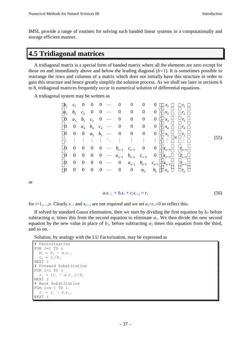
4.5 Tridiagonal matrices
A tridiagonal matrix is a special form of banded matrix where all the elements are zero except forthose on and immediately above and below the leading diagonal (b=1). It is sometimes possible torearrange the rows and columns of a matrix which does not initially have this structure in order togain this structure and hence greatly simplify the solution process. As we shall see later in sections 6to 8, tridiagonal matrices frequently occur in numerical solution of differential equations.
A tridiagonal system may be written as
b c
a b c
a b c
a b c
a b
b c
a b c
a b c
a b
n n
n n n
n n n
n n
1 1
2 2 2
3 3 3
4 4 4
5 5
3 3
2 2 2
1 1 1
0 0 0 0 0 0 0
0 0 0 0 0 0
0 0 0 0 0 0
0 0 0 0 0 0
0 0 0 0 0 0 0
0 0 0 0 0 0 0
0 0 0 0 0 0
0 0 0 0 0 0
0 0 0 0 0 0 0
L
L
L
L
L
M M M M M O M M M M
L
L
L
L
− −
− − −
− − −
=
−
−
−
−
−
−
x
x
x
x
x
x
x
x
x
r
r
r
r
r
r
r
r
r
n
n
n
n
n
n
n
n
1
2
3
4
5
3
2
1
1
2
3
4
5
3
2
1
M M(55)
or
aixi–1 + bixi + cixi+ 1 = ri (56)
for i=1,…,n. Clearly x–1 and xn+1 are not required and we set a1=cn=0 to reflect this.
If solved by standard Gauss elimination, then we start by dividing the first equation by b0 beforesubtracting a2 times this from the second equation to eliminate a2. We then divide the new secondequation by the new value in place of b2, before subtracting a3 times this equation from the third,and so on.
Solution, by analogy with the LU Factorisation, may be expressed as# FactorisationFOR i=1 TO n bi = bi – a ic i– 1
ci = ci /bi
NEXT i# Forward SubstitutionFOR i=1 TO n ri = (ri – a ir i– 1)/bi
NEXT i# Back SubstitutionFOR i=n– 1 TO 1 r i = r i – c ir i+1
NEXT i
Numerical Methods for Natural Sciences IB Introduction
– 38 –
4.6 Other approaches to solving linear systems
There are a number of other methods for solving general linear systems of equations includingapproximate iterative techniques. Many large matrices which need to be solved in practicalsituations have very special structures which allow solution - either exact or approximate - muchfaster than the general O(n3) solvers presented here. We shall return to this topic in section 8.1where we shall discuss a system with a special structure resulting from the numerical solution of theLaplace equation.
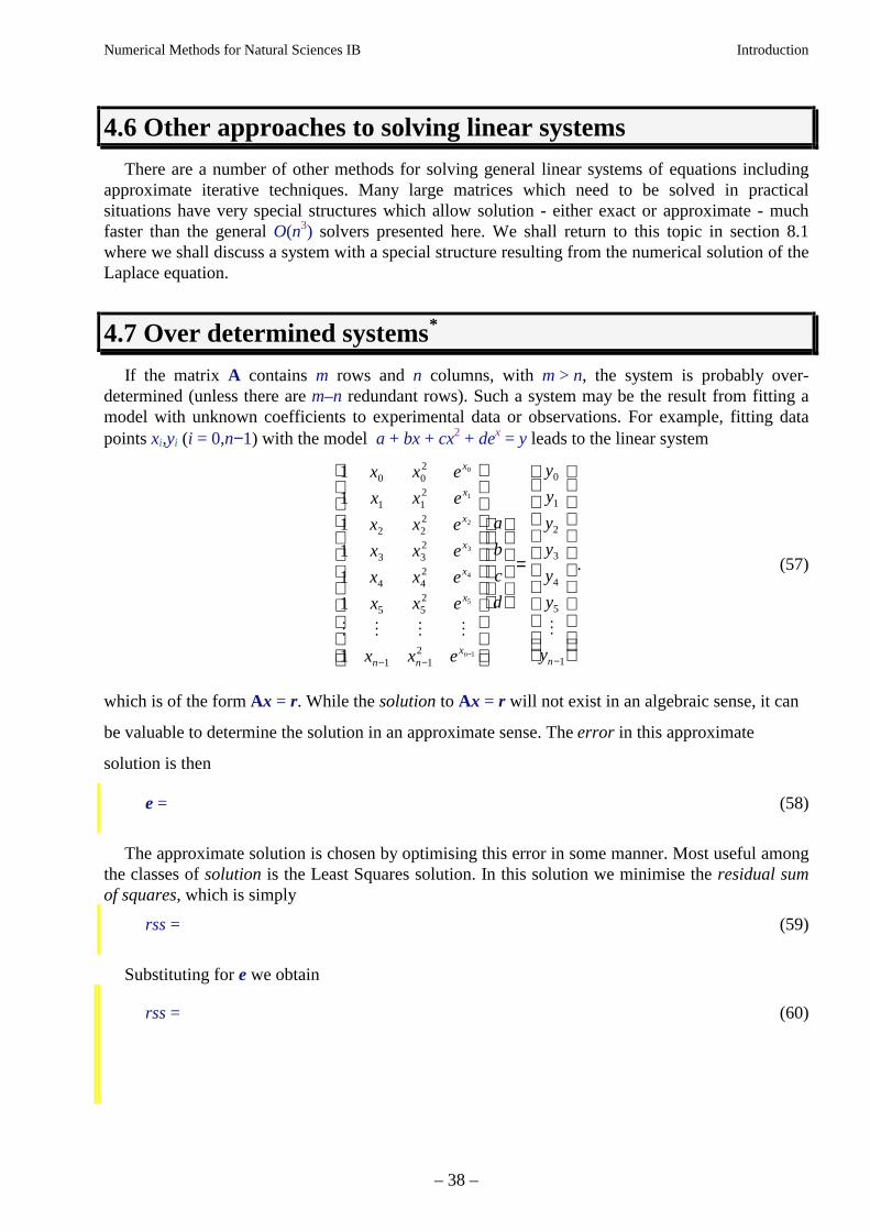
4.7 Over determined systems*
If the matrix A contains m rows and n columns, with m > n, the system is probably over-determined (unless there are m–n redundant rows). Such a system may be the result from fitting amodel with unknown coefficients to experimental data or observations. For example, fitting datapoints xi,yi (i = 0,n−1) with the model a + bx + cx2 + dex = y leads to the linear system
1
1
1
1
1
1
1
0 02
1 12
2 22
3 32
4 42
5 52
1 12
0
1
2
3
4
5
1
0
1
2
3
4
5
1
x x e
x x e
x x e
x x e
x x e
x x e
x x e
a
b
c
d
y
y
y
y
y
y
y
x
x
x
x
x
x
n nx
nn
M M M M M
− − −−
=
. (57)
which is of the form Ax = r. While the solution to Ax = r will not exist in an algebraic sense, it can
be valuable to determine the solution in an approximate sense. The error in this approximate
solution is then
e = (58)
The approximate solution is chosen by optimising this error in some manner. Most useful amongthe classes of solution is the Least Squares solution. In this solution we minimise the residual sumof squares, which is simply
rss = (59)
Substituting for e we obtain
rss = (60)
Numerical Methods for Natural Sciences IB Introduction
– 39 –
and setting ∂ ∂rss x to zero gives
∂∂rss
x=
(61)
Thus, if we solve the n by n problem ATAx = ATr, the solution vector x will give us the solution in aleast squares sense.
Warning: The matrix ATA is often poorly conditioned (nearly singular) and can lead tosignificant errors in the resulting Least Squares solution due to rounding error. While these errorsmay be reduced using pivoting in combination with Gauss Elimination, it is generally better to solvethe Least Squares problem using the Householder transformation, as this produces less roundingerror, or better still by Singular Value Decomposition which will highlight any redundant or nearlyredundant variables in x.
The Householder transformation avoids the poorly conditioned nature of ATA by solving theproblem directly without evaluating this matrix. Suppose Q is an orthogonal matrix such that
QTQ = I, (62)
where I is the identity matrix and Q is chosen to transform A into
QA =
, (63)
where R is a square matrix of a size n and 0 is a zero matrix of size m-n by n. The right-hand side ofthe system QAx = Qr becomes
Qr =b
c
, (64)
where b is a vector of size n and c is a vector of size m-n.
Now the turning point (global minimum) in the residual sum of squares, (61), this occurs when
[ ][ ]
∂∂rss
xx r
x r
= −
= −
2
2
A A A
A A A
T T
T T
(65)
* Not examinable
Numerical Methods for Natural Sciences IB Introduction
– 40 –
vanishes. For a non-trivial solution, that occurs when
Rx = b. (66)
This system may be solved to obtain the least squares solution x using any of the normal linearsolvers discussed above.
Further discussion of these methods is beyond the scope of this course.
4.8 Under determined systems*
If the matrix A contains m rows and n columns, with m < n, the system is under determined. Thesolution maps out a n–m dimensional subregion in n dimensional space. Solution of such systemstypically requires some form of optimisation in order to further constrain the solution vector.
Linear programming represents one method for solving such systems. In Linear Programming,the solution is optimised such that the objective function z=cTx is minimised. The “Linear” indicatesthat the underdetermined system of equations is linear and the objective function is linear in thesolution variable x. The “Programming” arose to enhance the chances of obtaining funding forresearch into this area when it was developing in the 1960s.
* Not examinable
Numerical Methods for Natural Sciences IB Introduction
– 41 –
5 Numerical integration
There are two main reasons for you to need to do numerical integration: analytical integrationmay be impossible or infeasible, or you may wish to integrate tabulated data rather than knownfunctions. In this section we outline the main approaches to numerical integration. Which ispreferable depends in part on the results required, and in part on the function or data to beintegrated.
5.1 Manual method
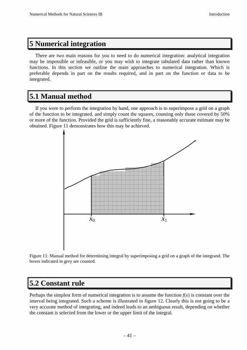
If you were to perform the integration by hand, one approach is to superimpose a grid on a graphof the function to be integrated, and simply count the squares, counting only those covered by 50%or more of the function. Provided the grid is sufficiently fine, a reasonably accurate estimate may beobtained. Figure 11 demonstrates how this may be achieved.
x1x0
Figure 11: Manual method for determining integral by superimposing a grid on a graph of the integrand. Theboxes indicated in grey are counted.
5.2 Constant rule
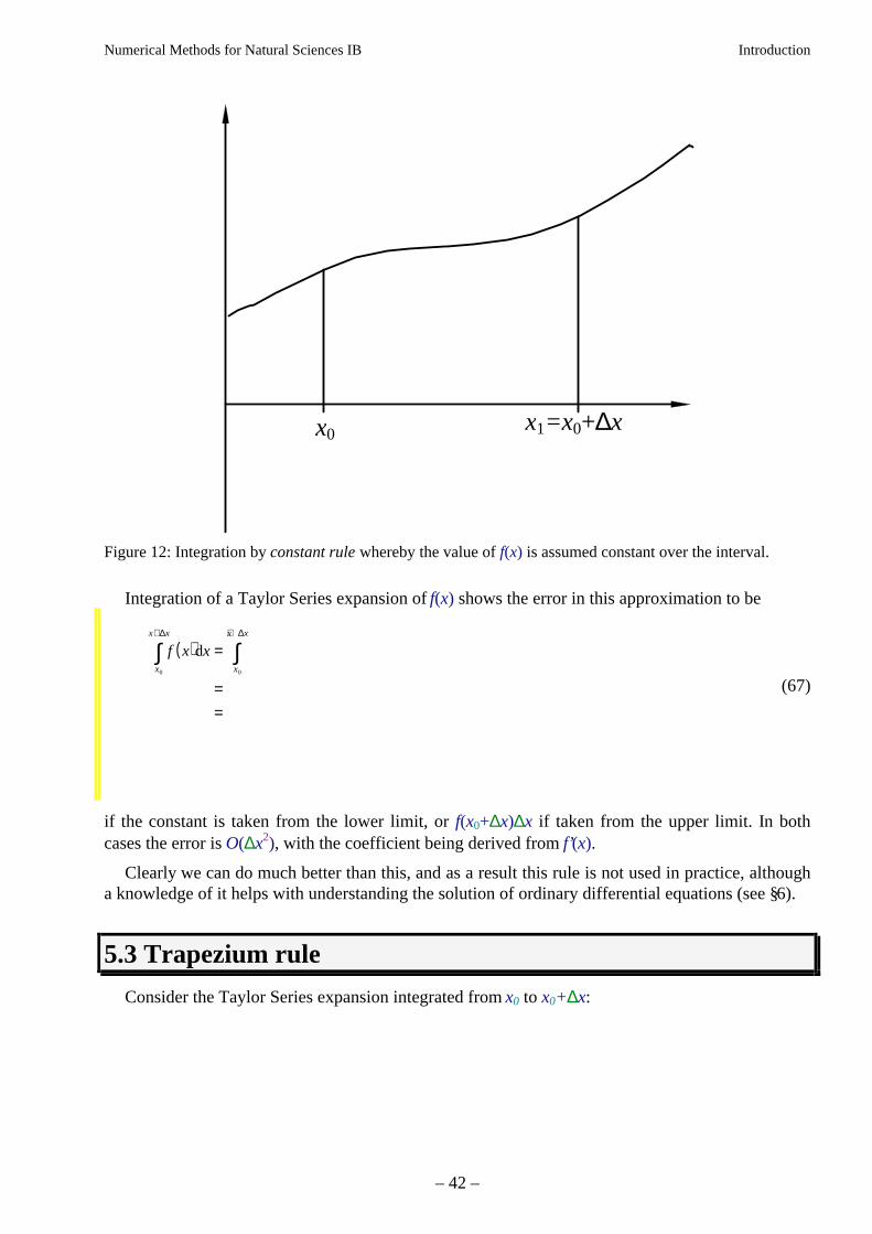
Perhaps the simplest form of numerical integration is to assume the function f(x) is constant over theinterval being integrated. Such a scheme is illustrated in figure 12. Clearly this is not going to be avery accurate method of integrating, and indeed leads to an ambiguous result, depending on whetherthe constant is selected from the lower or the upper limit of the integral.
Numerical Methods for Natural Sciences IB Introduction
– 42 –
x1=x0+∆xx0
Figure 12: Integration by constant rule whereby the value of f(x) is assumed constant over the interval.
Integration of a Taylor Series expansion of f(x) shows the error in this approximation to be
( )f x xx
x x
x
x x
d0 0
+ +
∫ ∫=
==
∆ ∆
(67)
if the constant is taken from the lower limit, or f(x0+∆x)∆x if taken from the upper limit. In bothcases the error is O(∆x2), with the coefficient being derived from f’(x).
Clearly we can do much better than this, and as a result this rule is not used in practice, althougha knowledge of it helps with understanding the solution of ordinary differential equations (see §6).
5.3 Trapezium rule
Consider the Taylor Series expansion integrated from x0 to x0+∆x:
Numerical Methods for Natural Sciences IB Introduction
– 43 –
( ) ( ) ( ) ( )
( ) ( ) ( )
f x x f x f x x f x x x
f x x f x x f x x
x
x x
x
x x
d d0 0
0 012 0
2
012 0
2 16 0
3
+ +
∫ ∫= + ′ + ′′ +
= + ′ + ′′ +=
∆ ∆
∆ ∆
∆ ∆ ∆
K
K . (68)
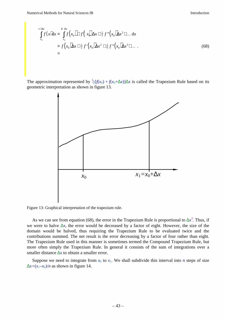
The approximation represented by 1/2[f(x0) + f(x0+∆x)]∆x is called the Trapezium Rule based on itsgeometric interpretation as shown in figure 13.
x1=x0+∆xx0
Figure 13: Graphical interpretation of the trapezium rule.
As we can see from equation (68), the error in the Trapezium Rule is proportional to ∆x3. Thus, ifwe were to halve ∆x, the error would be decreased by a factor of eight. However, the size of thedomain would be halved, thus requiring the Trapezium Rule to be evaluated twice and thecontributions summed. The net result is the error decreasing by a factor of four rather than eight.The Trapezium Rule used in this manner is sometimes termed the Compound Trapezium Rule, butmore often simply the Trapezium Rule. In general it consists of the sum of integrations over asmaller distance ∆x to obtain a smaller error.
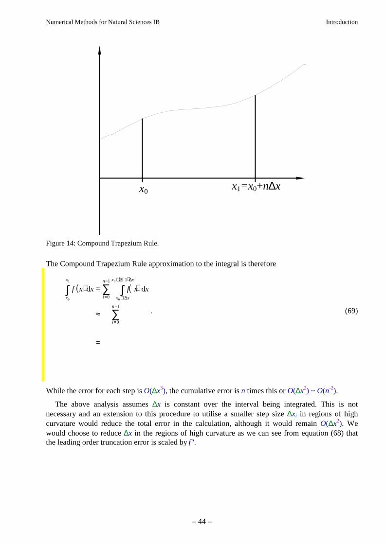
Suppose we need to integrate from x0 to x1. We shall subdivide this interval into n steps of size∆x=(x1–x0)/n as shown in figure 14.
Numerical Methods for Natural Sciences IB Introduction
– 44 –
x1=x0+n∆xx0
Figure 14: Compound Trapezium Rule.
The Compound Trapezium Rule approximation to the integral is therefore
( ) ( )( )
f x x f x xx
x
x i x
x i x
i
n
i
n
d d0
1
0
0 1
0
1
0
1
∫ ∫∑
∑
=
≈
=
+
+ +
=
−
=
−
∆
∆
. (69)
While the error for each step is O(∆x3), the cumulative error is n times this or O(∆x2) ~ O(n-2).
The above analysis assumes ∆x is constant over the interval being integrated. This is notnecessary and an extension to this procedure to utilise a smaller step size ∆xi in regions of highcurvature would reduce the total error in the calculation, although it would remain O(∆x2). Wewould choose to reduce ∆x in the regions of high curvature as we can see from equation (68) thatthe leading order truncation error is scaled by f".
Numerical Methods for Natural Sciences IB Introduction
– 45 –
5.4 Mid-point rule
A variant on the Trapezium Rule is obtained by integrating the Taylor Series from x0−∆x/2 tox0+∆x/2:
( ) ( ) ( ) ( )f x x f x f x x f x x xx x
x x
x x
x x
d d0
12
01
2
01
2
01
2
0 012 0
2
−
+
−
+
∫ ∫= + ′ + ′′ +
=∆
∆
∆
∆
∆ ∆ K. (70)
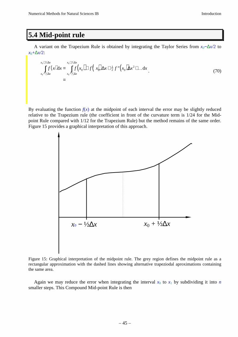
By evaluating the function f(x) at the midpoint of each interval the error may be slightly reducedrelative to the Trapezium rule (the coefficient in front of the curvature term is 1/24 for the Mid-point Rule compared with 1/12 for the Trapezium Rule) but the method remains of the same order.Figure 15 provides a graphical interpretation of this approach.
x0 + ½∆xx0 − ½∆x
Figure 15: Graphical interpretation of the midpoint rule. The grey region defines the midpoint rule as arectangular approximation with the dashed lines showing alternative trapeziodal aproximations containingthe same area.
Again we may reduce the error when integrating the interval x0 to x1 by subdividing it into nsmaller steps. This Compound Mid-point Rule is then
Numerical Methods for Natural Sciences IB Introduction
– 46 –
( )f x xx
x
i
n
d0
1
0
1
∫ ∑≈=
−
(71)
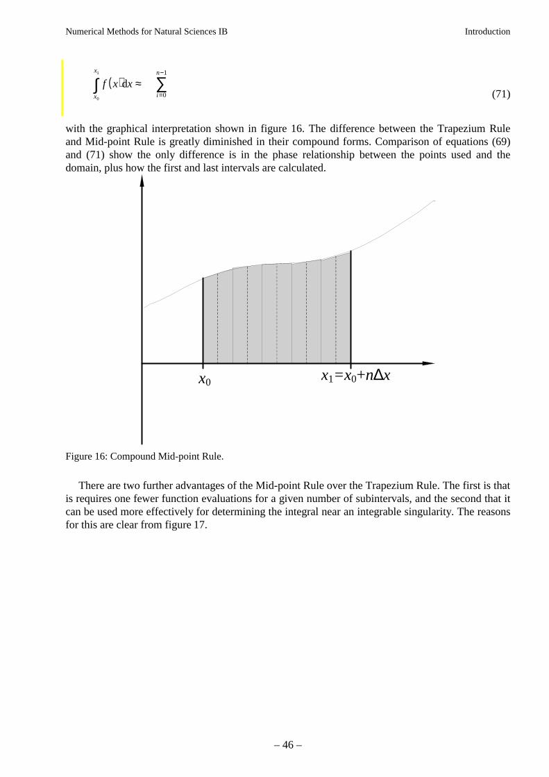
with the graphical interpretation shown in figure 16. The difference between the Trapezium Ruleand Mid-point Rule is greatly diminished in their compound forms. Comparison of equations (69)and (71) show the only difference is in the phase relationship between the points used and thedomain, plus how the first and last intervals are calculated.
x1=x0+n∆xx0
Figure 16: Compound Mid-point Rule.
There are two further advantages of the Mid-point Rule over the Trapezium Rule. The first is thatis requires one fewer function evaluations for a given number of subintervals, and the second that itcan be used more effectively for determining the integral near an integrable singularity. The reasonsfor this are clear from figure 17.

Numerical Methods for Natural Sciences IB Introduction
– 47 –
Figure 17: Applying the Midpoint Rule where the singular integrand would cause the Trapezium Rule tofail.
5.5 Simpson’s rule
An alternative approach to decreasing the step size ∆x for the integration is to increase theaccuracy of the functions used to approximate the integrand. Figure 18 sketches one possibility,using a quadratic approximation to f(x).
Figure 18: Quadratic approximation to integrand is the basis of Simpson’s Rule.
Integrating the Taylor series over an interval 2∆x shows

Numerical Methods for Natural Sciences IB Introduction
– 48 –
( )f x xx
x x
d0
2+
∫ =∆
(72)
[( )
( ) ( ) ( ) ( ) ( )( )( ) ( ) ( ) ( ) ( )( )
( ) ]
=
+ + ′ + ′′ + ′′′ + +
+ + ′ + ′′ + ′′′ + +
−
=
∆
∆ ∆ ∆ ∆
∆ ∆ ∆ ∆
∆
x
f x
f x f x x f x x f x x f x x
f x f x x f x x f x x f x x
f x x
iv
iv
iv
3
4
2 2
0
0 012 0
2 16 0
3 124 0
4
0 0 02 4
3 03 2
3 04
1730 0
4
K
K
K
Whereas the error in the Trapezium rule was O(∆x3), Simpson’s rule is two orders more accurate atO(∆x5), giving exact integration of cubics.
To improve the accuracy when integrating over larger intervals, the interval x0 to x1 may again besubdivided into n steps. The three-point evaluation for each subinterval requires that there are aneven number of subintervals. Hence we must be able to express the number of intervals as n=2m.The Compound Simpson’s rule is then
( ) ( ) ( )( ) ( )( )f x xx
f x i x f x i x f x i xx
x
i
m
d0
1
32 4 2 1 2 20 0 0
0
1
∫ ∑≈ + + + + + + +
=
=
−∆∆ ∆ ∆
(73)
and the corresponding error O(n∆x5) or O(∆x4).
5.6 Quadratic triangulation*
Simpson’s Rule may be employed in a manual way to determine the integral with nothing morethan a ruler. The approach is to cover the domain to be integrated with a triangle or trapezium(whichever is geometrically more appropriate) as is shown in figure 19. The integrand may cross theside of the trapezium (triangle) connecting the end points. For each arc-like region so created (thereare two in figure 19) the maximum deviation (indicated by arrows in figure 19) from the line shouldbe measured, as should the length of the chord joining the points of crossing. From Simpson’s rulewe may approximate the area between each of these arcs and the chord as
* Not examinable
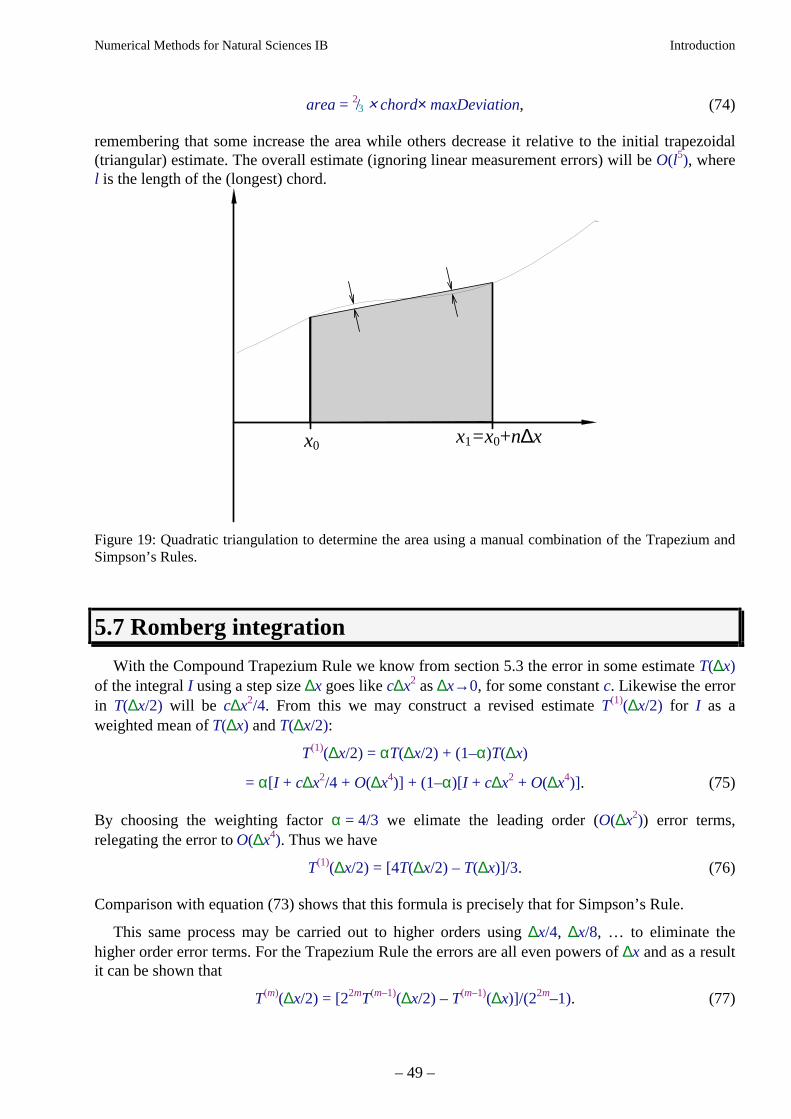
Numerical Methods for Natural Sciences IB Introduction
– 49 –
area = 2/3 × chord× maxDeviation, (74)
remembering that some increase the area while others decrease it relative to the initial trapezoidal(triangular) estimate. The overall estimate (ignoring linear measurement errors) will be O(l5), wherel is the length of the (longest) chord.
x1=x0+n∆xx0
Figure 19: Quadratic triangulation to determine the area using a manual combination of the Trapezium andSimpson’s Rules.
5.7 Romberg integration
With the Compound Trapezium Rule we know from section 5.3 the error in some estimate T(∆x)of the integral I using a step size ∆x goes like c∆x2 as ∆x→0, for some constant c. Likewise the errorin T(∆x/2) will be c∆x2/4. From this we may construct a revised estimate T(1)(∆x/2) for I as aweighted mean of T(∆x) and T(∆x/2):
T(1)(∆x/2) = αT(∆x/2) + (1–α)T(∆x)
= α[I + c∆x2/4 + O(∆x4)] + (1–α)[I + c∆x2 + O(∆x4)]. (75)
By choosing the weighting factor α = 4/3 we elimate the leading order (O(∆x2)) error terms,relegating the error to O(∆x4). Thus we have
T(1)(∆x/2) = [4T(∆x/2) – T(∆x)]/3. (76)
Comparison with equation (73) shows that this formula is precisely that for Simpson’s Rule.
This same process may be carried out to higher orders using ∆x/4, ∆x/8, … to eliminate thehigher order error terms. For the Trapezium Rule the errors are all even powers of ∆x and as a resultit can be shown that
T(m)(∆x/2) = [22mT(m–1)(∆x/2) – T(m–1)(∆x)]/(22m–1). (77)
Numerical Methods for Natural Sciences IB Introduction
– 50 –
A similar process may also be applied to the Compound Simpson’s Rule.
5.8 Gauss quadrature
By careful selection of the points at which the function is evaluated it is possible to increase theprecision for a given number of function evaluations. The Mid-point rule is an example of this: withjust a single function evaluation it obtains the same order of accuracy as the Trapezium Rule (whichrequires two points).
One widely used example of this is Gauss quadrature which enables exact integration of cubicswith only two function evaluations (in contrast Simpson’s Rule, which is also exact for cubics,requires three function evaluations). Gauss quadrature has the formula
( ) ( )f x xx
f x x f x x O xx
x x x
d0
1 0
2
1
2
3
6
1
2
3
60 04
= +
∫ ≈ + −
+ + +
+∆ ∆
∆ ∆ ∆ . (78)
In general it is possible to choose M function evaluations per interval to obtain a formula exact forall polynomials of degree 2M−1 and less.
The Gauss Quadrature accurate to order 2M−1 may be determined using the same approachrequired for the two-point scheme. This may be derived by comparing the Taylor Series expansionfor the integral with that for the points x0+α∆x and x0+β∆x:
( ) ( ) ( ) ( ) ( ) ( )
( ) ( ) ( ) ( ) ( ) ( )
( ) ( ) ( ) ( ) ( ) ( )
( ) ( ) ( )
f x x xf xx
f xx
f xx
f x O x
xf x xf x
xf x
xf x
f x xf xx
f xx
f x
xf xx
f x
x
x x x
d0
1 0
0
2
0
3
0
4
05
0 0
2
0
3
0
0 0
2
0
3
0
0
2
02
2 6 24
2 2 6
2 6
2
= +
∫ = + ′ + ′′ + ′′′ +
= + ′ + ′′ + ′′′ +
+ + ′ + ′′ + ′′′ +
= + + ′ +
∆
∆∆ ∆ ∆
∆
∆
∆∆
α∆α∆ α∆
β∆β∆ β∆
α β α
K
K
( ) ( )+ + + +β α β23
3 34
4 12
∆ ∆x xK
. (79)
Equating the various terms reveals
(80)
the solution of which gives the positions stated in equation (78).
Using three function evaluations: symmetry suggests for the interval x0−∆x to x0+∆x the pointsshould be evaluated at x0 and x0±α with weightings 2∆xA and 2∆xB. The Taylor Series expansion ofthe integral gives
( ) ( ) ( ) ( ) ( ) ( )f x x x f xx
f xx
f xx
f x O xx x
x x
iv vid0
0
26 120 50400
2
0
4
0
6
08
−
+
∫ = + ′′ + + +
∆
∆
∆∆ ∆ ∆
∆ , (81)
while the expansion of the function for the three points gives

Numerical Methods for Natural Sciences IB Introduction
– 51 –
( ) ( ) ( ) ( )[ ][
( )( )( )( )]
f x x x Af x Bf x Bf x
x Af
B f f f f f f f f O
B f f f f f f f f O
x x
x x
iv v vi vii
iv v vi vii
d0
0
2
2
0 0 0
12
2 16
3 124
4 1120
5 1720
6 15040
7 8
12
2 16
3 124
4 1120
5 1720
6 15040
7 8
−
+
∫ = + − + +
=
+ − ′ + ′′ − ′′′ + − + − +
+ + ′ + ′′ + ′′′ + + + + +
∆
∆
∆
∆
α α
α α α α α α α α
α α α α α α α α
( ) ( )[ ]= + + ′′ + + +2 2 2 112
4 1360
6 8∆x A B f B f B f f Oiv viα α α α . (82)
Comparing the terms between (81) and (82) gives
A + 2B = 1
Bα2 = ∆x2/6
Bα4/12 = ∆x4/120 (83)
which may be solved to obtain the position of the evaluations and the weightings
(Bα4/12)/Bα2 = (∆x4/120) / (∆x2/6)
⇒ α2 = (6/10)∆x2
⇒ α = (3/5)1/2∆x
B = 5/18
A = 4/9, (84)
thus
( ) ( )f x x x f x f x x f x xx x
x x
d0
0 1
98 5
3
55
3
50 0
1 2
0
1 2
−
+
∫ = + −
+ +
∆
∆
∆ ∆ ∆/ /
. (85)
5.9 Example of numerical integration
Consider the integral
sin x x d0
2π
∫ = , (86)
which may be integrated numerically using any of the methods described in the previous sections.Tables 2 to 6 summarise the error in the numerical estimates for the Trapezium Rule, MidpointRule, Simpson’s Rule, Gauss Quadrature and a three point Gauss Quadrature (formula derived inlectures). Table 7 compares these errors. The results are presented in terms of the number offunction evaluations required. The calculations were performed in double precision.
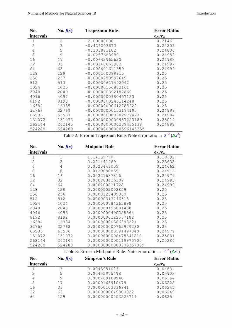
Numerical Methods for Natural Sciences IB Introduction
– 52 –
No.intervals
No. f(x) Trapezium Rule Error Ratio:e2n/en
1 2 -2.00000000 0.21462 3 -0.429203673 0.242034 5 -0.103881102 0.248068 9 -0.0257683980 0.2495216 17 -0.00642965622 0.2498832 33 -0.00160663902 0.2499764 65 -0.000401611359 0.24999128 129 -0.000100399815 0.25256 257 -0.0000250997649 0.25512 513 -0.00000627492942 0.251024 1025 -0.00000156873161 0.252048 2049 -0.000000392182860 0.254096 4097 -0.0000000980457133 0.258192 8193 -0.0000000245114248 0.2516384 16385 -0.00000000612785222 0.2532768 32769 -0.00000000153194190 0.2499965536 65537 -0.000000000382977427 0.24994131072 131073 -0.0000000000957223189 0.25014262144 262145 -0.0000000000239435138 0.24898524288 524289 -0.00000000000596145355
Table 2: Error in Trapezium Rule. Note error ratio → 2−2 (∆x2)
No.intervals
No. f(x) Midpoint Rule Error Ratio:e2n/en
1 1 1.14189790 0.193922 2 0.221441469 0.236384 4 0.0523443059 0.246628 8 0.0129090855 0.2491616 16 0.00321637816 0.2497932 32 0.000803416309 0.2499564 64 0.000200811728 0.24999128 128 0.0000502002859 0.25256 256 0.0000125499060 0.25512 512 0.00000313746618 0.251024 1024 0.000000784365898 0.252048 2048 0.000000196091438 0.254096 4096 0.0000000490228564 0.258192 8192 0.0000000122557182 0.2516384 16384 0.00000000306393221 0.2532768 32768 0.000000000765979280 0.2565536 65536 0.000000000191497040 0.24979131072 131072 0.0000000000478341810 0.25081262144 262144 0.0000000000119970700 0.25286524288 524288 0.00000000000303357339
Table 3: Error in Mid-point Rule. Note error ratio → 2−2 (∆x2)
No.intervals
No. f(x) Simpson’s Rule Error Ratio:e2n/en
1 3 0.0943951023 0.04832 5 0.00455975498 0.059034 9 0.000269169948 0.061648 17 0.0000165910479 0.0622816 33 0.00000103336941 0.0624532 65 0.0000000645300022 0.0624964 129 0.00000000403225719 0.0625
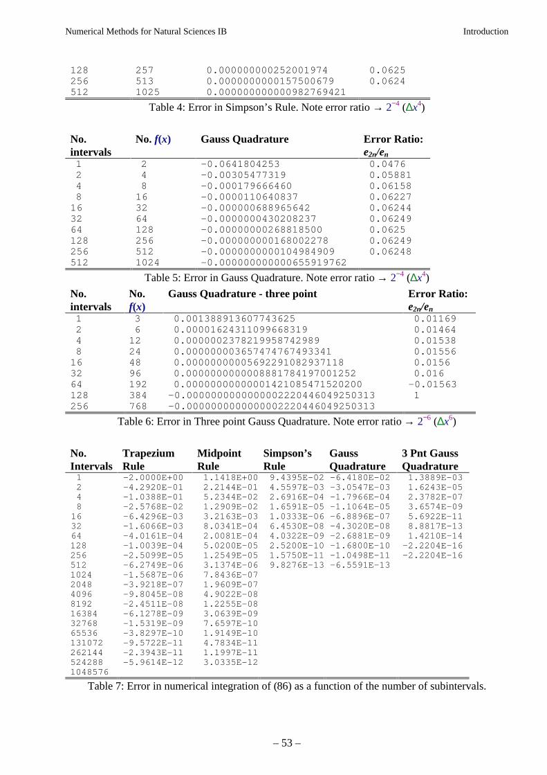
Numerical Methods for Natural Sciences IB Introduction
– 53 –
128 257 0.000000000252001974 0.0625256 513 0.0000000000157500679 0.0624512 1025 0.000000000000982769421
Table 4: Error in Simpson’s Rule. Note error ratio → 2−4 (∆x4)
No.intervals
No. f(x) Gauss Quadrature Error Ratio:e2n/en
1 2 -0.0641804253 0.04762 4 -0.00305477319 0.058814 8 -0.000179666460 0.061588 16 -0.0000110640837 0.0622716 32 -0.000000688965642 0.0624432 64 -0.0000000430208237 0.0624964 128 -0.00000000268818500 0.0625128 256 -0.000000000168002278 0.06249256 512 -0.0000000000104984909 0.06248512 1024 -0.000000000000655919762
Table 5: Error in Gauss Quadrature. Note error ratio → 2−4 (∆x4)
No.intervals
No.f(x)
Gauss Quadrature - three point Error Ratio:e2n/en
1 3 0.001388913607743625 0.011692 6 0.00001624311099668319 0.014644 12 0.0000002378219958742989 0.015388 24 0.000000003657474767493341 0.0155616 48 0.00000000005692291082937118 0.015632 96 0.0000000000008881784197001252 0.01664 192 0.00000000000001421085471520200 -0.01563128 384 -0.0000000000000002220446049250313 1256 768 -0.0000000000000002220446049250313
Table 6: Error in Three point Gauss Quadrature. Note error ratio → 2−6 (∆x6)
No.Intervals
TrapeziumRule
MidpointRule
Simpson’sRule
GaussQuadrature
3 Pnt GaussQuadrature
1 -2.0000E+00 1.1418E+00 9.4395E-02 -6.4180E-02 1.3889E-032 -4.2920E-01 2.2144E-01 4.5597E-03 -3.0547E-03 1.6243E-054 -1.0388E-01 5.2344E-02 2.6916E-04 -1.7966E-04 2.3782E-078 -2.5768E-02 1.2909E-02 1.6591E-05 -1.1064E-05 3.6574E-09
16 -6.4296E-03 3.2163E-03 1.0333E-06 -6.8896E-07 5.6922E-1132 -1.6066E-03 8.0341E-04 6.4530E-08 -4.3020E-08 8.8817E-1364 -4.0161E-04 2.0081E-04 4.0322E-09 -2.6881E-09 1.4210E-14128 -1.0039E-04 5.0200E-05 2.5200E-10 -1.6800E-10 -2.2204E-16256 -2.5099E-05 1.2549E-05 1.5750E-11 -1.0498E-11 -2.2204E-16512 -6.2749E-06 3.1374E-06 9.8276E-13 -6.5591E-131024 -1.5687E-06 7.8436E-072048 -3.9218E-07 1.9609E-074096 -9.8045E-08 4.9022E-088192 -2.4511E-08 1.2255E-0816384 -6.1278E-09 3.0639E-0932768 -1.5319E-09 7.6597E-1065536 -3.8297E-10 1.9149E-10131072 -9.5722E-11 4.7834E-11262144 -2.3943E-11 1.1997E-11524288 -5.9614E-12 3.0335E-121048576
Table 7: Error in numerical integration of (86) as a function of the number of subintervals.
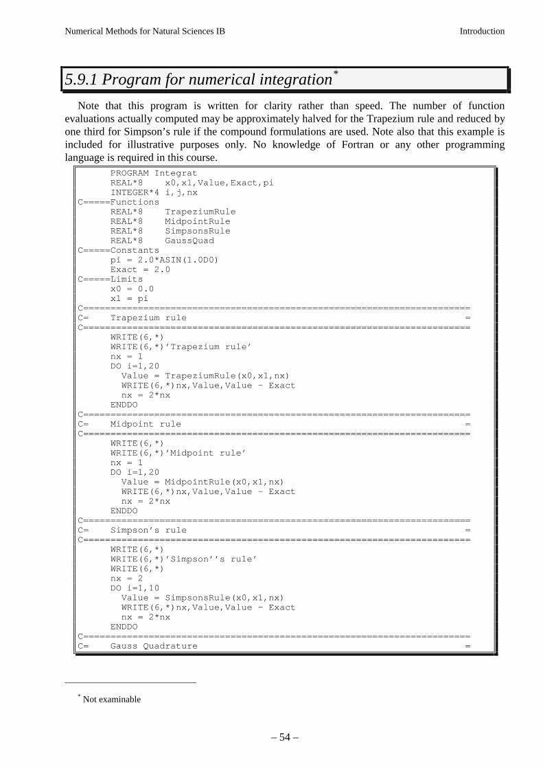
Numerical Methods for Natural Sciences IB Introduction
– 54 –
5.9.1 Program for numerical integration*
Note that this program is written for clarity rather than speed. The number of functionevaluations actually computed may be approximately halved for the Trapezium rule and reduced byone third for Simpson’s rule if the compound formulations are used. Note also that this example isincluded for illustrative purposes only. No knowledge of Fortran or any other programminglanguage is required in this course.
PROGRAM Integrat REAL*8 x0,x1,Value,Exact,pi INTEGER*4 i,j,nxC=====Functions REAL*8 TrapeziumRule REAL*8 MidpointRule REAL*8 SimpsonsRule REAL*8 GaussQuadC=====Constants pi = 2.0*ASIN(1.0D0) Exact = 2.0C=====Limits x0 = 0.0 x1 = piC=======================================================================C= Trapezium rule =C======================================================================= WRITE(6,*) WRITE(6,*)’Trapezium rule’ nx = 1 DO i=1,20 Value = TrapeziumRule(x0,x1,nx) WRITE(6,*)nx,Value,Value - Exact nx = 2*nx ENDDOC=======================================================================C= Midpoint rule =C======================================================================= WRITE(6,*) WRITE(6,*)’Midpoint rule’ nx = 1 DO i=1,20 Value = MidpointRule(x0,x1,nx) WRITE(6,*)nx,Value,Value - Exact nx = 2*nx ENDDOC=======================================================================C= Simpson’s rule =C======================================================================= WRITE(6,*) WRITE(6,*)’Simpson’’s rule’ WRITE(6,*) nx = 2 DO i=1,10 Value = SimpsonsRule(x0,x1,nx) WRITE(6,*)nx,Value,Value - Exact nx = 2*nx ENDDOC=======================================================================C= Gauss Quadrature =
* Not examinable
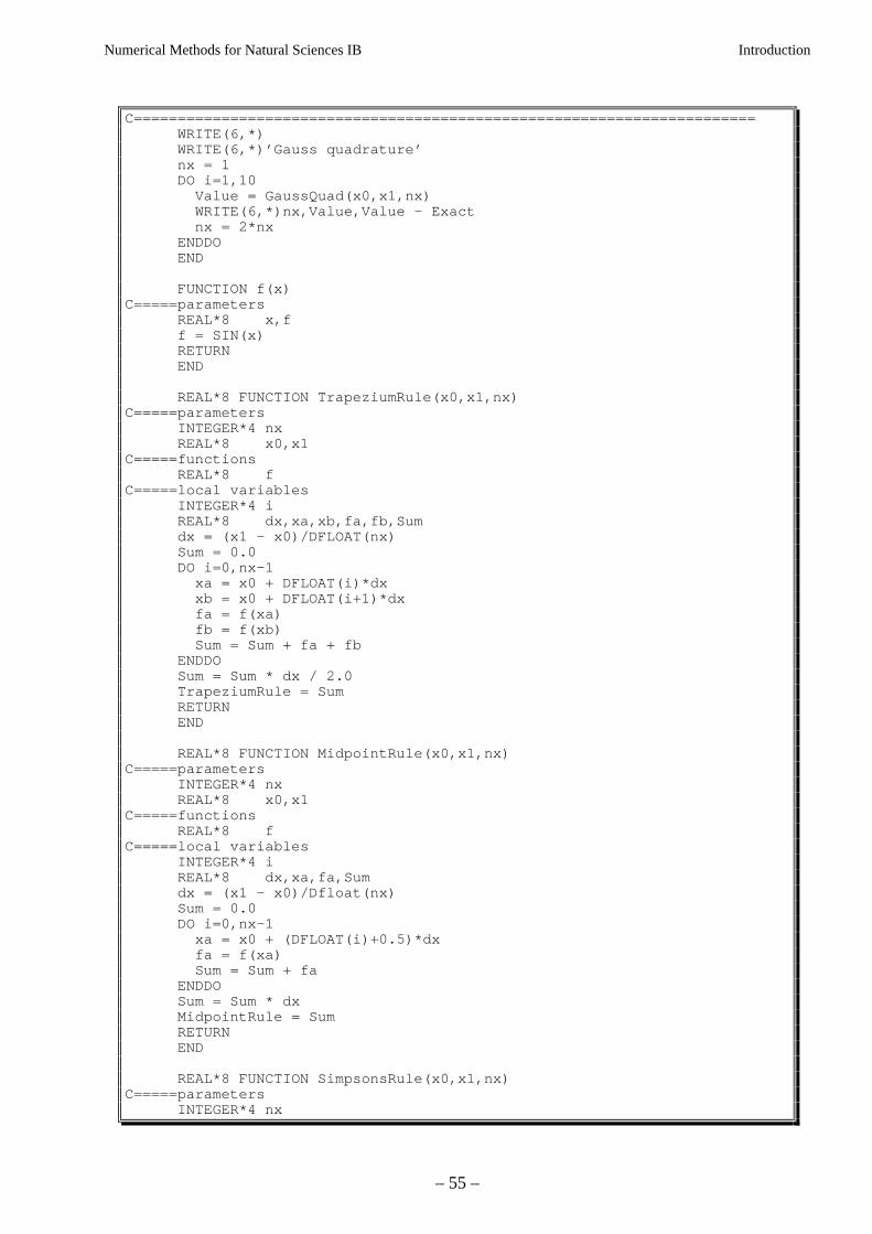
Numerical Methods for Natural Sciences IB Introduction
– 55 –
C======================================================================= WRITE(6,*) WRITE(6,*)’Gauss quadrature’ nx = 1 DO i=1,10 Value = GaussQuad(x0,x1,nx) WRITE(6,*)nx,Value,Value - Exact nx = 2*nx ENDDO END
FUNCTION f(x)C=====parameters REAL*8 x,f f = SIN(x) RETURN END
REAL*8 FUNCTION TrapeziumRule(x0,x1,nx)C=====parameters INTEGER*4 nx REAL*8 x0,x1C=====functions REAL*8 fC=====local variables INTEGER*4 i REAL*8 dx,xa,xb,fa,fb,Sum dx = (x1 - x0)/DFLOAT(nx) Sum = 0.0 DO i=0,nx-1 xa = x0 + DFLOAT(i)*dx xb = x0 + DFLOAT(i+1)*dx fa = f(xa) fb = f(xb) Sum = Sum + fa + fb ENDDO Sum = Sum * dx / 2.0 TrapeziumRule = Sum RETURN END
REAL*8 FUNCTION MidpointRule(x0,x1,nx)C=====parameters INTEGER*4 nx REAL*8 x0,x1C=====functions REAL*8 fC=====local variables INTEGER*4 i REAL*8 dx,xa,fa,Sum dx = (x1 - x0)/Dfloat(nx) Sum = 0.0 DO i=0,nx-1 xa = x0 + (DFLOAT(i)+0.5)*dx fa = f(xa) Sum = Sum + fa ENDDO Sum = Sum * dx MidpointRule = Sum RETURN END
REAL*8 FUNCTION SimpsonsRule(x0,x1,nx)C=====parameters INTEGER*4 nx
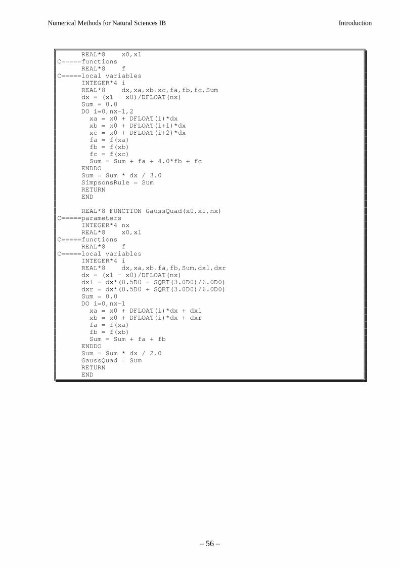
Numerical Methods for Natural Sciences IB Introduction
– 56 –
REAL*8 x0,x1C=====functions REAL*8 fC=====local variables INTEGER*4 i REAL*8 dx,xa,xb,xc,fa,fb,fc,Sum dx = (x1 - x0)/DFLOAT(nx) Sum = 0.0 DO i=0,nx-1,2 xa = x0 + DFLOAT(i)*dx xb = x0 + DFLOAT(i+1)*dx xc = x0 + DFLOAT(i+2)*dx fa = f(xa) fb = f(xb) fc = f(xc) Sum = Sum + fa + 4.0*fb + fc ENDDO Sum = Sum * dx / 3.0 SimpsonsRule = Sum RETURN END
REAL*8 FUNCTION GaussQuad(x0,x1,nx)C=====parameters INTEGER*4 nx REAL*8 x0,x1C=====functions REAL*8 fC=====local variables INTEGER*4 i REAL*8 dx,xa,xb,fa,fb,Sum,dxl,dxr dx = (x1 - x0)/DFLOAT(nx) dxl = dx*(0.5D0 - SQRT(3.0D0)/6.0D0) dxr = dx*(0.5D0 + SQRT(3.0D0)/6.0D0) Sum = 0.0 DO i=0,nx-1 xa = x0 + DFLOAT(i)*dx + dxl xb = x0 + DFLOAT(i)*dx + dxr fa = f(xa) fb = f(xb) Sum = Sum + fa + fb ENDDO Sum = Sum * dx / 2.0 GaussQuad = Sum RETURN END
Numerical Methods for Natural Sciences IB Introduction
– 57 –
6 First order ordinary differential equations
Ths section of the course introduces some commonly used methods for determining thenumerical solutions of ordinary differential equations. These methods will then be used in §8 as thebasis for solving some types of partial differential equations.
6.1 Taylor series
The key idea behind numerical solution of odes is the combination of function values at differentpoints or times to approximate the derivatives in the required equation. The manner in which thefunction values are combined is determined by the Taylor Series expansion for the point at whichthe derivative is required. This gives us a finite difference approximation to the derivative.
6.2 Finite difference
Consider a first order ode of the form
d
d
y
t=
(87)
subject to some boundary/initial condition y(t=t0) = c. The finite difference solution of this equationproceeds by discretising the independent variable t to t0, t0+∆t, t0+2∆t, t0+3∆t, … We shall denotethe exact solution at some t = tn = t0+n∆t by yn = y(t=tn) and our approximate solution by Yn. Wethen look to solve
(88)
at each of the points in the domain, where Y’n is an approximation to dy/dt based on the discrete setof Yn.
If we take the Taylor Series expansion for the grid points in the neighbourhood of some pointt = tn,
...
Yn-2 =
Yn-1 =
Yn =
Yn+1 =
Yn+2 =
... (89)
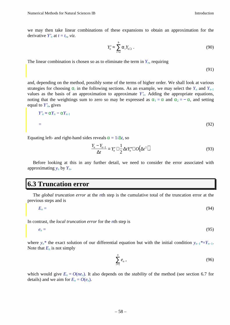
Numerical Methods for Natural Sciences IB Introduction
– 58 –
we may then take linear combinations of these expansions to obtain an approximation for thederivative Y’n at t = tn, viz.
′ ≈ +=∑Y Yn i n ii a
b
α . (90)
The linear combination is chosen so as to eliminate the term in Yn, requiring
(91)
and, depending on the method, possibly some of the terms of higher order. We shall look at variousstrategies for choosing αi in the following sections. As an example, we may select the Yn and Yn-1
values as the basis of an approximation to approximate Y’n. Adding the appropriate equations,noting that the weightings sum to zero so may be expressed as α1 = α and α2 = − α, and settingequal to Y’n, gives
Y’n ≈ αYn − αYn-1
= (92)
Equating left- and right-hand sides reveals α = 1/∆t, so
( )Y Y
tY tY O tn n
n n
−= ′ + ′′+−1 21
2∆∆ ∆ . (93)
Before looking at this in any further detail, we need to consider the error associated withapproximating yn by Yn.
6.3 Truncation error
The global truncation error at the nth step is the cumulative total of the truncation error at theprevious steps and is
En = (94)
In contrast, the local truncation error for the nth step is
en = (95)
where yn* the exact solution of our differential equation but with the initial condition yn–1*=Yn–1.Note that En is not simply
eni
n
=∑
1
, (96)
which would give En = O(nen). It also depends on the stability of the method (see section 6.7 fordetails) and we aim for En = O(en).
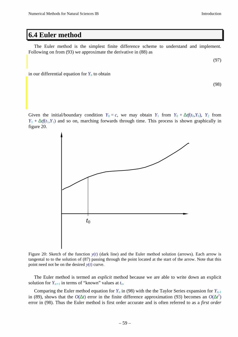
Numerical Methods for Natural Sciences IB Introduction
– 59 –
6.4 Euler method
The Euler method is the simplest finite difference scheme to understand and implement.Following on from (93) we approximate the derivative in (88) as
(97)
in our differential equation for Yn to obtain
(98)
Given the initial/boundary condition Y0 = c, we may obtain Y1 from Y0 + ∆tf(t0,Y0), Y2 fromY1 + ∆tf(t1,Y1) and so on, marching forwards through time. This process is shown graphically infigure 20.
t0
Figure 20: Sketch of the function y(t) (dark line) and the Euler method solution (arrows). Each arrow istangental to to the solution of (87) passing through the point located at the start of the arrow. Note that thispoint need not be on the desired y(t) curve.
The Euler method is termed an explicit method because we are able to write down an explicitsolution for Yn+1 in terms of “known” values at tn.
Comparing the Euler method equation for Yn in (98) with the the Taylor Series expansion for Yn-1
in (89), shows that the O(∆t) error in the finite difference approximation (93) becomes an O(∆t2)error in (98). Thus the Euler method is first order accurate and is often referred to as a first order
Numerical Methods for Natural Sciences IB Introduction
– 60 –
method. Moreover, it can be shown that if Yn=yn+O(∆t2), then Yn+1=yn+1+O(∆t2) provided thescheme is stable (see section 6.7).
6.5 Implicit methods
The Euler method outlined in the previous section may be summarised by the update formulaYn+1 = g(Yn,tn,∆t). In contrast implicit methods have have Yn+1 on both sides: Yn+1 = h(Yn,Yn+1,tn,∆t),for example. Such implicit methods are computationally more expensive for a single step thanexplicit methods, but offer advantages in terms of stability and/or accuracy in many circumstances.Often the computational expense per step is more than compensated for by it being possible to takelarger steps (see section 6.7).
6.5.1 Backward Euler
The backward Euler method is almost identical to its explicit relative, the only difference beingthat the derivative Y’n is approximated by
Y'n ≈ (99)
to give the evolution equation
Yn+1 = (100)
This is shown graphically in figure 21.
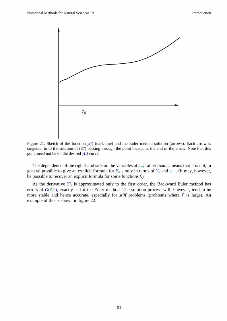
Numerical Methods for Natural Sciences IB Introduction
– 61 –
t0
Figure 21: Sketch of the function y(t) (dark line) and the Euler method solution (arrows). Each arrow istangental to to the solution of (87) passing through the point located at the end of the arrow. Note that thispoint need not be on the desired y(t) curve.
The dependence of the right-hand side on the variables at tn+1 rather than tn means that it is not, ingeneral possible to give an explicit formula for Yn+1 only in terms of Yn and tn+1. (It may, however,be possible to recover an explicit formula for some functions f.)
As the derivative Y’n is approximated only to the first order, the Backward Euler method haserrors of O(∆t2), exactly as for the Euler method. The solution process will, however, tend to bemore stable and hence accurate, especially for stiff problems (problems where f’ is large). Anexample of this is shown in figure 22.

Numerical Methods for Natural Sciences IB Introduction
– 62 –
t0
Backward Euler
(Forward) Euler
Crank-Nicholson
Figure 22: Comparison of ordinary differential equation solvers for a stiff problem.
6.5.2 Richardson extrapolation
The Romberg integration approach (presented in section 5.7) of using two approximations ofdifferent step size to construct a more accurate estimate may also be used for numerical solution ofordinary differential equations. Again, if we have the estimate for some time t calculated using atime step ∆t, then for both the Euler and Backward Euler methods the approximate solution isrelated to the true solution by Y(t,∆t) = y(t) + c∆t2. Similarly an estimate using a step size ∆t/2 willfollow Y(t,∆t/2) = y(t) + 1/4c∆t2 as ∆t→0. Combining these two estimates to try and cancel theO(∆t2) errors gives the improved estimate as
Y(1)(t,∆t/2) = [4Y(t,∆t/2) – Y(t,∆t) ]/3. (101)
The same approach may be applied to higher order methods such as those presented in thefollowing sections. It is generally preferable, however, to utilise a higher order method to start with,the exception being that calculating both Y(t,∆t) and Y(t,∆t/2) allows the two solutions to becompared and thus the trunctation error estimated.
6.5.3 Crank-Nicholson
If we use central differences rather than the forward difference of the Euler method or thebackward difference of the backward Euler, we may obtain a second order method due tocancellation of the terms of O(∆t2). Using the same discretisation of t we obtain
(102)
Numerical Methods for Natural Sciences IB Introduction
– 63 –
Substitution into our differential equation for Yn gives
(103)
The requirement for f(tn+1/2,Yn+1/2) is then satisfied by a linear interpolation for f between tn–1/2 andtn+1/2 to obtain
Yn+1 − Yn = (104)
As with the Backward Euler, the method is implicit and it is not, in general, possible to write anexplicit expression for Yn+1 in terms of Yn.
Formal proof that the Crank-Nicholson method is second order accurate is slightly morecomplicated than for the Euler and Backward Euler methods due to the linear interpolation toapproximate f(tn+1/2,Yn+1/2). The overall approach is much the same, however, with a requirement forTaylor Series expansions about tn::
( )y ydy
dtt
d y
dtt O tn n+ = + + +
=
1
2
22 31
2∆ ∆ ∆ (105a)
( )f t yn n+ + =1 1,
(105b)
Substitution of these into the left- and right-hand sides of equation (104) reveals
( )y y f tf
tf
f
yt O tn n n+ − = + +
+1
2 31
2∆ ∆ ∆
∂∂
∂∂
(106a)
and
( ) ( )( ) ( )
( )
1
2
1
2
1
2
1 12
2 3
f t y f t y t f ff
tf
f
yt O t t
f tf
tf
f
yt O t
n n n n n n
n
, ,+ = + + +
+
= + +
+
+ + ∆ ∆ ∆ ∆
∆ ∆ ∆
∂∂
∂∂
∂∂
∂∂
(106b)
which are equal up to O(∆t3).
Numerical Methods for Natural Sciences IB Introduction
– 64 –
6.6 Multistep methods
As an alternative, the accuracy of the approximation to the derivative may be improved by usinga linear combination of additional points. By utilising only Yn–s+1,Yn–s+2,…,Yn we may construct anapproximation to the derivatives of orders 1 to s at tn. For example, if s = 2 then
Y’n =
Y"n ≈ (107)
and so we may construct a second order method from the Taylor series expansion as
Yn+1 = Yn + ∆tY’n + ½∆t2Y"n
= (108)
For s=3 we also have Y’"n and so can make use of a second-order one-sided finite difference toapproximate Y"n = f’n = (3fn -4 fn-1 + fn-2)/2∆t and include the third order Y’"n = f"n = (fn-2fn-1+fn-2)/∆t2 to obtain
Yn+1 = Yn + ∆tY’n + 1/2∆t2Y"n + 1/6∆t3Y"n
= (109)
These methods are called Adams-Bashforth methods. Note that s = 1 recovers the Euler method.
Implicit Adams-Bashforth methods are also possible if we use information about fn+1 in additionto earlier time steps. The corresponding s = 2 method then uses
Y’n = fn,
Y"n ≈
Y’"n ≈ (110)
to give
Yn+1 = Yn + ∆tY’n + 1/2∆t2Y"n + 1/6∆t3Y’"n
= Yn + (1/12)∆t(5fn+1 + 8fn – fn–1). (111)
This family of implicit methods is known as Adams-Moulton methods.
6.7 Stability
The stability of a method can be even more important than its accuracy as measured by the orderof the truncation error. Suppose we are solving
(112)
Numerical Methods for Natural Sciences IB Introduction
– 65 –
for some complex λ. The exact solution is bounded (i.e. does not increase without limit) providedReλ ≤ 0. Substituting this into the Euler method shows
Yn+1 = Yn + ∆t f(tn,Yn)
=
(113)
If Yn is to remain bounded for increasing n and given Reλ < 0 we require
(114)
If we choose a time step ∆t which does not satisfy (114) then Yn will increase without limit. Thiscondition (114) on ∆t is very restrictive if λ<<0 as it demonstrates the Euler method must use verysmall time steps ∆t < 2|λ|–1 if the solution is to converge on y = 0.
The reason why we consider the behaviour of equation (112) is that it is a model for thebehaviour of small errors. Suppose that at some stage during the solution process our approximatesolution is
y$ = (115)
where ε is the (small) error. Substituting this into our differential equation of the form y’ = f(t,y) andusing a Taylor Series expansion gives
( )
dy
dt
dy
dt
d
dt
f t y
$
$,
= +
==
ε
(116)
Thus, to the leading order, the error obeys an equation of the form given by (112), with λ = ∂f/∂y.As it is desirable for errors to decrease (and thus the solution remain stable) rather than increase(and the solution be unstable), the limit on the time step suggested by (114) applies for theapplication of the Euler method to any ordinary differential equation. A consequence of the decay oferrors present at one time step as the solution process proceeds is that memory of a particular timestep’s contribution to the global truncation error decays as the solution advances through time. Thusthe global truncation error is dominated by the local trunction error(s) of the most recent step(s) andO(En) = O(en).
Numerical Methods for Natural Sciences IB Introduction
– 66 –
In comparison, solution of (112) by the Backward Euler method
Yn+1 = Yn + ∆t f(tn+1,Yn+1)
= (117)
can be rearranged for Yn+1 and
Yn+1 = (118)
which will be stable provided
(119)
For Reλ ≤ 0 this is always satisfied and so the Backward Euler method is unconditionally stable.
The Crank-Nicholson method may be analysed in a similar fashion with
(1-λ∆t/2)Yn+1 = (1+λ∆t/2)Yn, (120)
to arrive at
Yn+1 = [(1+λ∆t/2)/(1 – λ∆t/2)]n+1 Y0, (121)
with the magnitude of the term in square brackets always less than unity for Reλ < 0. Thus, likeBackward Euler, Crank-Nicholson is unconditionally stable.
In general, explicit methods require less computation per step, but are only conditionally stableand so may require far smaller step sizes than an implicit method of nominally the same order.
6.8 Predictor-corrector methods
One approach to using an implicit method is to use a direct iteration to solve the implicitequation. For example, the Backward Euler method has the form
Yn+1 = (122)
Applying the theory for direct iteration outlined in §3.6, we may write
Yn+1,i = (123)
setting Yn+1,0 = Yn, and iterate over i until the solution has converged. From (21) we know it willconverge if
(124)
Numerical Methods for Natural Sciences IB Introduction
– 67 –
and the solution will gradually approach the Backward Euler solution. Note that this convergencecriterion is more stringent than the stability criterion established in §6.7!
What we are effectively doing here is making a prediction with the Euler method (our equationfor Yn+1,1 is just the Euler method), then multiple corrections to this to get the solution to convergeon the Backward Euler method. A similar strategy may be applied to the Crank-Nicholson methodto obtain
Yn+1,i = (125)
requiring ½ ∆t ∂f/∂Y < 1 for convergence. Once convergence is achieved, we are left with a second-order implicit scheme. However, it may not be necessary or desirable to carry on iterating untilconvergence is achieved. Moreover, the condition for convergence using (125) imposes the samerestrictions upon ∆t as stability of the Euler method. There are other reasons, however, for takingthis approach.
The above examples, if iterated only a finite number of times rather than until convergence isachieved, belong to a class of methods known as predictor-corrector methods. Predictor-correctormethods try to combine the advantages of the simplicity of explicit methods with the improvedaccuracy of implicit methods. They achieve this by using an explicit method to predict the solutionYn+1
(p) at tn+1 and then utilise f(tn+1,Yn+1(p)) as an approximation to f(tn+1,Yn+1) to correct this
prediction using something similar to an implicit step.
6.8.1 Improved Euler method
The simplest of these methods combines the Euler method as the predictor
Yn+1(1) = (126)
and then the Backward Euler to give the corrector
Yn+1(2) = (127)
The final solution is the mean of these:
Yn+1 = (128)
To understand the stability of this method we again use the y’ = λy so that the three stepsdescribed by equations (126) to (128) become
Yn+1(1) = Yn + λ∆tYn, (129a)
Yn+1(2) = Yn + λ∆tYn+1
(1)
=
=, (129b)
Numerical Methods for Natural Sciences IB Introduction
– 68 –
Yn+1 = (Yn+1(1) + Yn+1
(2))/2
=
=
= (129c)
Stability requires |1 + λ∆t + 1/2λ2∆t2| < 1 (for Reλ < 0) which in turn restricts ∆t < 2|λ|–1. Thus thestability of this method, commonly known as the Improved Euler method, is identical to the Eulermethod. It is also the same as the criterion for the iterative Crank-Nicholson method given in (125)to converge. This is not surprising as it is limited by the stability of the initial predictive step. Theaccuracy of the method is, however, second order as may be seen by comparison of (129c) with theTaylor Series expansion.
6.8.2 Runge-Kutta methods
The Improved Euler method is the simplest of a family of similar predictor corrector methodsfollowing the form of a single predictor step and one or more corrector steps. The corrector stepmay be repeated a fixed number of times, or until the estimate for Yn+1 converges to some tolerance.
One subgroup of this family are the Runge-Kutta methods which use a fixed number of correctorsteps. The Improved Euler method is the simplest of this subgroup. Perhaps the most widely used ofthese is the fourth order method:
Yn+1 − Yn = k = ∆t f(t,Y)
k(1) = ∆tf(tn,Yn) , (130a)
k(2) = ∆tf(tn+1/2∆t ,Yn+½k(1)) , (130b)
k(3) = ∆tf(tn+1/2∆t ,Yn+½k(2)) , (130c)
k(4) = ∆tf(tn+∆t ,Yn+k(3)) , (130d)
Yn+1 = Yn + (k(1) + 2k(2) + 2k(3) + k(4))/6. (130e)
In order to analyse this we need to construct Taylor-Series expansions fork(2) = ∆tf(tn+
1/2∆t,Yn+1/2k
(1)) = ∆t[f(tn,Yn)+(∆t/2)(∂f/∂t+f∂f/∂y)], and similarly for k(3) and k(4). This isthen compared with a full Taylor-Series expansion for Yn+1 up to fourth order. To achieve this werequire
Y" = df/dt
= ∂f/∂t + ∂y/∂t ∂f/∂y
= (131)

Numerical Methods for Natural Sciences IB Introduction
– 69 –
Y’" = d2f/dt2
= ∂2f/∂t2 + 2f ∂2f/∂t∂y + ∂f/∂t ∂f/∂y + f2 ∂2f/∂y2 + f (∂f/∂y)2, (132)
Y"" =
and similarly for Y"". All terms up to order ∆t4 can be shown to match, with the error coming in at∆t5.
Numerical Methods for Natural Sciences IB Introduction
– 70 –
7 Higher order ordinary differential equations
In this section we look at how to solve higher order ordinary differential equations. Some of thetechniques discussed here are based on the techniques introduced in §6, and some rely on acombination of this material and the linear algebra of §4.
7.1 Initial value problems
The discussion so far has been for first order ordinary differential equations. All the methodsgiven may be applied to higher ordinary differential equations, provided it is possible to write anexplicit expression for the highest order derivative and the system has a complete set of initialconditions. Consider some equation
(133)
where at t = t0 we know the values of y, dy/dt, d2y/dt2, …, dn-1y/dtn-1. By writing x0=y, x1=dy/dt,x2=d2y/dt2, …, xn–1=dn–1y/dtn–1, we may express this as the system of equations
x0’ =
x1’ =
x2’ =
. . . .
xn–2’ =
xn–1’ = (134)
and use the standard methods for updating each xi for some tn+1 before proceeding to the next timestep. A decision needs to be made as to whether the values of xi for tn or tn+1 are to be used on theright hand side of the equation for xn–1’ . This decision may affect the order and convergence of themethod. Detailed analysis may be undertaken in a manner similar to that for the first order ordinarydifferential equations.
7.2 Boundary value problems
For second (and higher) order odes, two (or more) initial/boundary conditions are required. Ifthese two conditions do not correspond to the same point in time/space, then the simple extension ofthe first order methods outlined in section 7.1 can not be applied without modification. There aretwo relatively simple approaches to solve such equations.
Numerical Methods for Natural Sciences IB Introduction
– 71 –
7.2.1 Shooting method
Suppose we are solving a second order equation of the form y" = f(t,y,y’) subject to y(0) = c0 andy(1) = c1. With the shooting method we apply the y(0)=c0 boundary condition and make some guessthat y’(0) = α0. This gives us two initial conditions so that we may apply the simple time-steppingmethods already discussed in section 7.1. The calculation proceeds until we have a value for y(1). Ifthis does not satisfy y(1) = c1 to some acceptable tolerance, we revise our guess for y’(0) to somevalue α1, say, and repeat the time integration to obtain an new value for y(1). This process continuesuntil we hit y(1)=c1 to the acceptable tolerance. The number of iterations which will need to bemade in order to achieve an acceptable tolerance will depend on how good the refinement algorithmfor α is. We may use the root finding methods discussed in section 3 to undertake this refinement.
The same approach can be applied to higher order ordinary differential equations. For a system oforder n with m boundary conditions at t = t0 and n–m boundary conditions at t = t1, we will requireguesses for n–m initial conditions. The computational cost of refining these n–m guesses willrapidly become large as the dimensions of the space increase.
7.2.2 Linear equations
The alternative is to rewrite the equations using a finite difference approximation with step size∆t = (t1–t0)/N to produce a system of N+1 simultaneous equations. Consider the second order linearsystem
(135)
with boundary conditions y(t0) = α and y(t1) + y’(t1) = β. If we use the central differenceapproximations
y'i = (136a)
y"i = (136b)
Substitution into (135) gives
(137)
and we may write the boundary condition at t = t0 as
(138)
For t = t1 we must express the derivative in the boundary condition in finite difference form usingpoints that exist in our mesh. The obvious thing to do is to take the backward difference so that theboundary condition becomes
(139)
Numerical Methods for Natural Sciences IB Introduction
– 72 –
but as we shall see, this choice is not ideal.
The above strategy leads to the system of equations
…
(140)
This tridiagonal system may be readily solved using the method discussed in section 4.5.
There is one problem with the scheme outlined above: while the Y" and Y’ derivatives within thedomain are second order accurate, the boundary condition at t = t1 is imposed only as a first-orderapproximation to the derivative. We have two ways in which we may improve the accuracy of thisboundary condition.
The first way is the most obvious: make use of the Yn-2 value to construct a second-orderapproximation to Y" so that we have
(141)
so that the last equation in our system becomes
(142)
The problem with this is that we then loose our simple tridiagonal system.
The second approach is to artificially increase the size of the domain by one mesh point andimpose the boundary condition inside the domain. The additional mesh point is often referred to as adummy mesh point or dummy cell. This leads to the last three equations being
(1+1/2a∆t)Yn–2 + (b∆t2–2)Yn–1 + (1–1/2a∆t)Yn = c∆t2,
(143)
The attraction of this approach is that we maintain our simple tri-diagonal system.
Clearly the same tricks can be applied if we have a boundary condition on the derivative at t0.
Numerical Methods for Natural Sciences IB Introduction
– 73 –
Higher order linear equations may be catered for in a similar manner and the matrix representingthe system of equations will remain banded, but not as sparse as tridiagonal. The solution may beundertaken using the modified LU decomposition introduced in section 4.4.
Nonlinear equations may also be solved using this approach, but will require an iterative solutionof the resulting matrix system Ax = b as the matrix A will be a function of x. In most circumstancesthis is most efficiently achieved through a Newton-Raphson algorithm, similar in principle to thatintroduced in section 3.4 but where a system of linear equations requires solution for each iteration.
7.3 Other considerations*
Not examinable
7.3.1 Truncation error*
Not examinable
7.3.2 Error and step control*
Not examinable
* Not examinable* Not examinable* Not examinable
Numerical Methods for Natural Sciences IB Introduction
– 74 –
8 Partial differential equations
In this section we shall concentrate on the numerical solution of second order linear partialdifferential equations.
8.1 Laplace equation
Consider the Laplace equation in two dimensions
(144)
in some rectangular domain described by x in [x0,x1], y in [y0,y1]. Suppose we discretise the solutionϕ onto a m+1 by n+1 rectangular grid (or mesh) given by
xi = (145a)
yj = (145b)
where i=0,m, j=0,n. The mesh spacing is ∆x = (x1–x0)/m and ∆y = (y1–y0)/n. Let
ϕij = (146)
be the exact solution at the mesh point i,j , and Φij ≈ ϕij be the approximate solution at that meshpoint.
By considering the Taylor Series expansion for ϕ about some mesh point i,j,
ϕi+1,j = (147a)
ϕi-1,j = (147b)
ϕi,j+1 = (147c)
ϕi,j-1 = (147d)
it is clear that we may approximate ∂2ϕ/∂x2 and ∂2ϕ/∂y2to the second order using the four adjacentmesh points to obtain the finite difference approximation
(148)
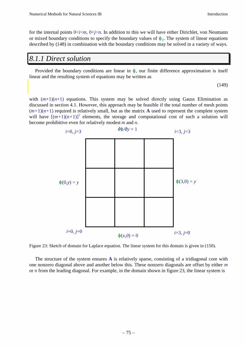
Numerical Methods for Natural Sciences IB Introduction
– 75 –
for the internal points 0<i<m, 0<j<n. In addition to this we will have either Dirichlet, von Neumannor mixed boundary conditions to specify the boundary values of ϕij. The system of linear equationsdescribed by (148) in combination with the boundary conditions may be solved in a variety of ways.
8.1.1 Direct solution
Provided the boundary conditions are linear in ϕ, our finite difference approximation is itselflinear and the resulting system of equations may be written as
(149)
with (m+1)(n+1) equations. This system may be solved directly using Gauss Elimination asdiscussed in section 4.1. However, this approach may be feasible if the total number of mesh points(m+1)(n+1) required is relatively small, but as the matrix A used to represent the complete systemwill have [(m+1)(n+1)]2 elements, the storage and computational cost of such a solution willbecome prohibitive even for relatively modest m and n.
i=0, j=0 i=3, j=0
i=0, j=3 i=3, j=3
ϕ(x,0) = 0
∂ϕ/∂y = 1
ϕ(0,y) = y ϕ(3,0) = y
Figure 23: Sketch of domain for Laplace equation. The linear system for this domain is given in (150).
The structure of the system ensures A is relatively sparse, consisting of a tridiagonal core withone nonzero diagonal above and another below this. These nonzero diagonals are offset by either mor n from the leading diagonal. For example, in the domain shown in figure 23, the linear system is
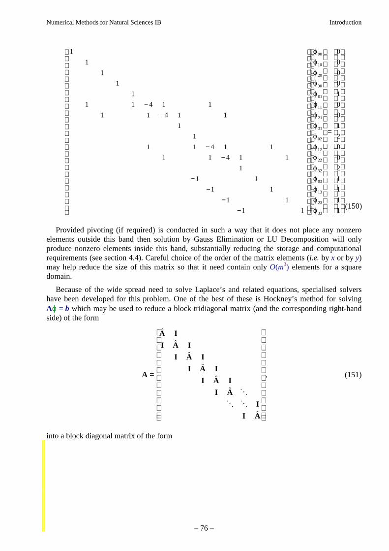
Numerical Methods for Natural Sciences IB Introduction
– 76 –
1
1
1
1
1
1 1 4 1 1
1 1 4 1 1
1
1
1 1 4 1 1
1 1 4 1 1
1
1 1
1 1
1 1
1 1
00
10
20
30
01
11
21
31
02
12
22
32
03
13
23
33
−−
−−
−−
−−
ϕϕϕϕϕϕϕϕϕϕϕϕϕϕϕϕ
=
0
0
0
0
1
0
0
1
2
0
0
2
1
1
1
1(150)
Provided pivoting (if required) is conducted in such a way that it does not place any nonzeroelements outside this band then solution by Gauss Elimination or LU Decomposition will onlyproduce nonzero elements inside this band, substantially reducing the storage and computationalrequirements (see section 4.4). Careful choice of the order of the matrix elements (i.e. by x or by y)may help reduce the size of this matrix so that it need contain only O(m3) elements for a squaredomain.
Because of the wide spread need to solve Laplace’s and related equations, specialised solvershave been developed for this problem. One of the best of these is Hockney’s method for solvingAϕ = b which may be used to reduce a block tridiagonal matrix (and the corresponding right-handside) of the form
A
A I
I A I
I A I
I A I
I A I
I A
I
I A
=
$
$
$
$
$
$
$
O
O O
, (151)
into a block diagonal matrix of the form
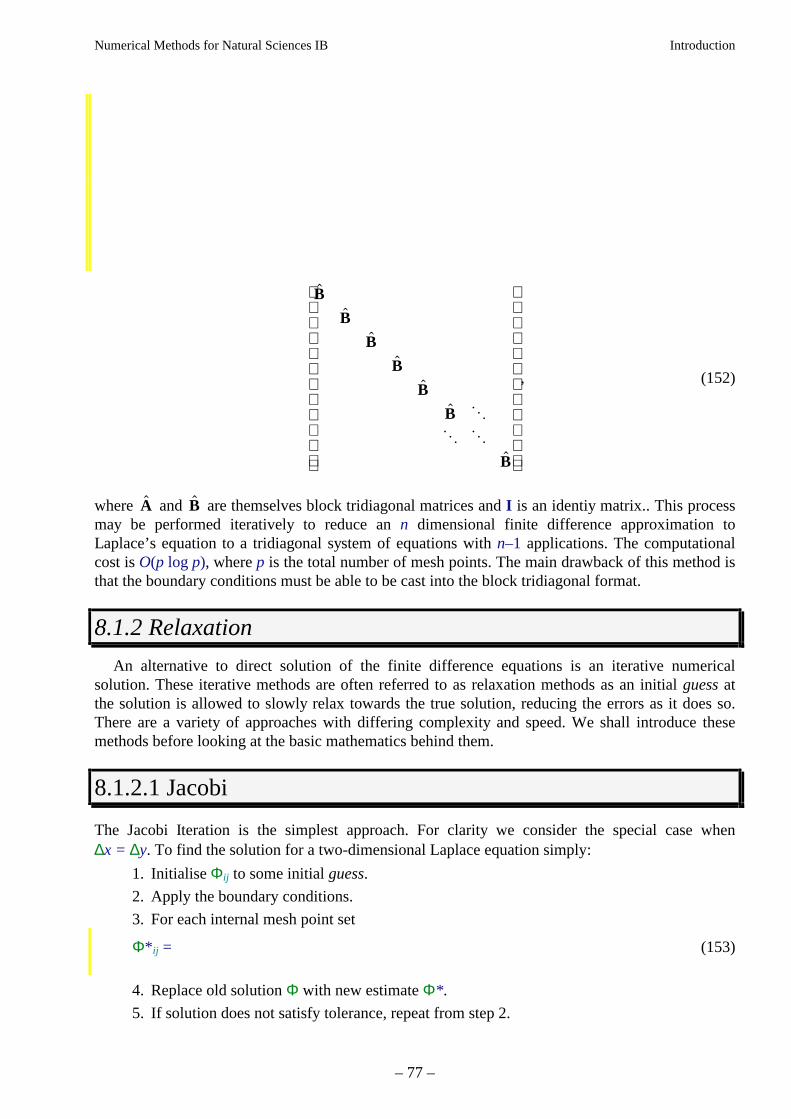
Numerical Methods for Natural Sciences IB Introduction
– 77 –
$
$
$
$
$
$
$
B
B
B
B
B
B
B
O
O O
, (152)
where $A and $B are themselves block tridiagonal matrices and I is an identiy matrix.. This processmay be performed iteratively to reduce an n dimensional finite difference approximation toLaplace’s equation to a tridiagonal system of equations with n–1 applications. The computationalcost is O(p log p), where p is the total number of mesh points. The main drawback of this method isthat the boundary conditions must be able to be cast into the block tridiagonal format.
8.1.2 Relaxation
An alternative to direct solution of the finite difference equations is an iterative numericalsolution. These iterative methods are often referred to as relaxation methods as an initial guess atthe solution is allowed to slowly relax towards the true solution, reducing the errors as it does so.There are a variety of approaches with differing complexity and speed. We shall introduce thesemethods before looking at the basic mathematics behind them.
8.1.2.1 Jacobi
The Jacobi Iteration is the simplest approach. For clarity we consider the special case when∆x = ∆y. To find the solution for a two-dimensional Laplace equation simply:
1. Initialise Φij to some initial guess.
2. Apply the boundary conditions.
3. For each internal mesh point set
Φ*ij = (153)
4. Replace old solution Φ with new estimate Φ* .
5. If solution does not satisfy tolerance, repeat from step 2.
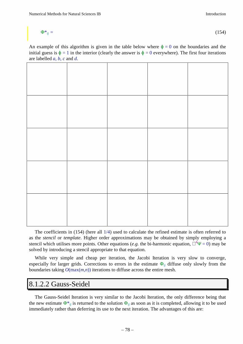
Numerical Methods for Natural Sciences IB Introduction
– 78 –
Φ* ij = (154)
An example of this algorithm is given in the table below where ϕ = 0 on the boundaries and theinitial guess is ϕ = 1 in the interior (clearly the answer is ϕ = 0 everywhere). The first four iterationsare labelled a, b, c and d.
The coefficients in (154) (here all 1/4) used to calculate the refined estimate is often referred toas the stencil or template. Higher order approximations may be obtained by simply employing astencil which utilises more points. Other equations (e.g. the bi-harmonic equation, ∇4Ψ = 0) may besolved by introducing a stencil appropriate to that equation.
While very simple and cheap per iteration, the Jacobi Iteration is very slow to converge,especially for larger grids. Corrections to errors in the estimate Φij diffuse only slowly from theboundaries taking O(max(m,n)) iterations to diffuse across the entire mesh.
8.1.2.2 Gauss-Seidel
The Gauss-Seidel Iteration is very similar to the Jacobi Iteration, the only difference being thatthe new estimate Φ* ij is returned to the solution Φij as soon as it is completed, allowing it to be usedimmediately rather than deferring its use to the next iteration. The advantages of this are:
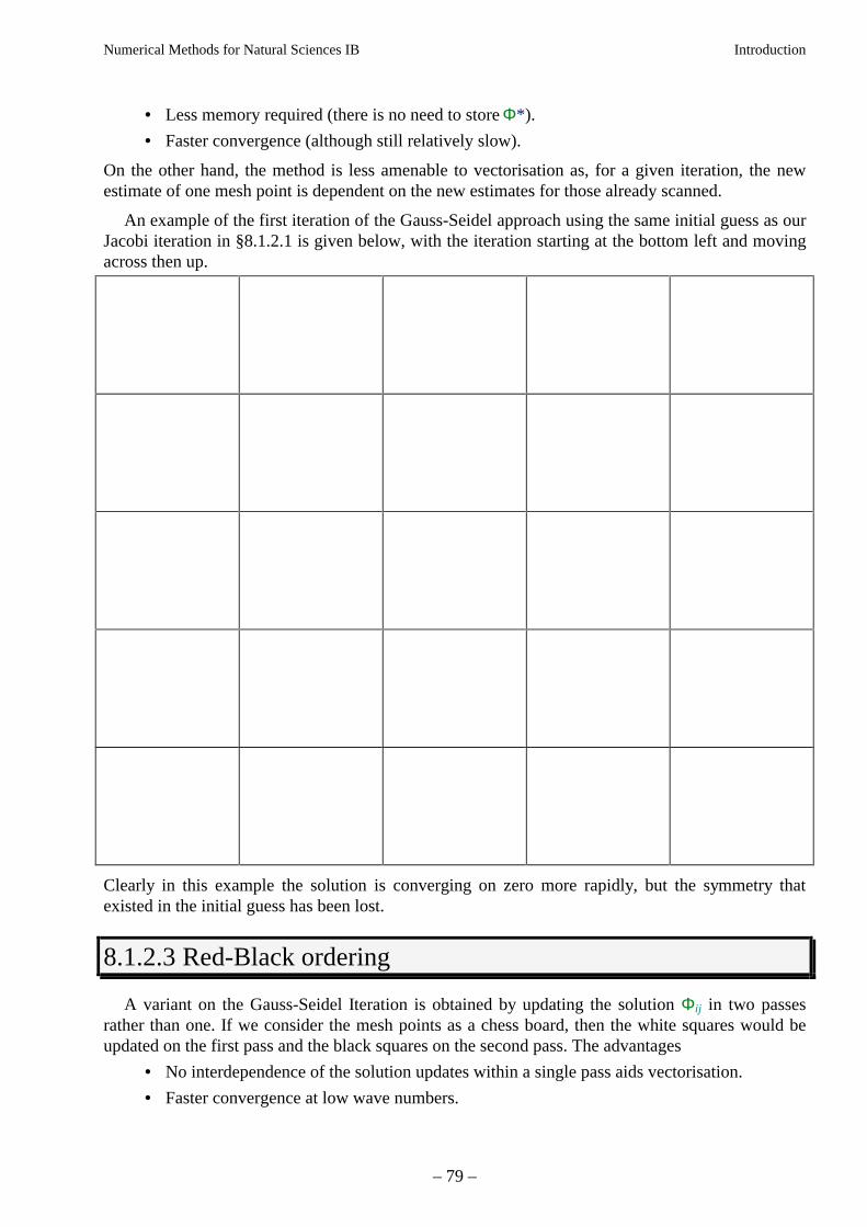
Numerical Methods for Natural Sciences IB Introduction
– 79 –
• Less memory required (there is no need to store Φ* ).
• Faster convergence (although still relatively slow).
On the other hand, the method is less amenable to vectorisation as, for a given iteration, the newestimate of one mesh point is dependent on the new estimates for those already scanned.
An example of the first iteration of the Gauss-Seidel approach using the same initial guess as ourJacobi iteration in §8.1.2.1 is given below, with the iteration starting at the bottom left and movingacross then up.
Clearly in this example the solution is converging on zero more rapidly, but the symmetry thatexisted in the initial guess has been lost.
8.1.2.3 Red-Black ordering
A variant on the Gauss-Seidel Iteration is obtained by updating the solution Φij in two passesrather than one. If we consider the mesh points as a chess board, then the white squares would beupdated on the first pass and the black squares on the second pass. The advantages
• No interdependence of the solution updates within a single pass aids vectorisation.
• Faster convergence at low wave numbers.
Numerical Methods for Natural Sciences IB Introduction
– 80 –
An example, based on those in the previous two sections, is given below. Note that the cellslabelled “Red” are updated on the first pass and those labelled “Black” on the second pass. Unlikethe Gauss-Seidel, the order in which the cells are updated within one pass does not matter.
In this example the solution is converging faster than the Jacobi iteration and at a comparablerate to Gauss-Seidel, yet is maintaining the symmetries which existed in the initial guess. For manyproblems, particularly those looking at instabilities, the maintenance of symmetries is important.
8.1.2.4 Successive Over Relaxation (SOR)
It has been found that the errors in the solution obtained by any of the three preceding methodsdecrease only slowly and often decrease in a monotonic manner. Hence, rather than setting
Φ* ij = (Φi+1,j + Φi–1,j + Φi,j+1 + Φi,j–1)/4,
for each internal mesh point, we use
Φ*ij = (155)
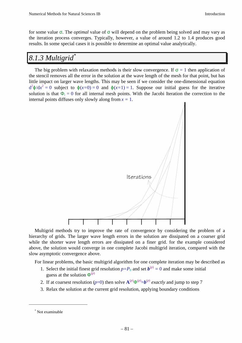
Numerical Methods for Natural Sciences IB Introduction
– 81 –
for some value σ. The optimal value of σ will depend on the problem being solved and may vary asthe iteration process converges. Typically, however, a value of around 1.2 to 1.4 produces goodresults. In some special cases it is possible to determine an optimal value analytically.
8.1.3 Multigrid*
The big problem with relaxation methods is their slow convergence. If σ = 1 then application ofthe stencil removes all the error in the solution at the wave length of the mesh for that point, but haslittle impact on larger wave lengths. This may be seen if we consider the one-dimensional equationd2ϕ/dx2 = 0 subject to ϕ(x=0) = 0 and ϕ(x=1) = 1. Suppose our initial guess for the iterativesolution is that Φi = 0 for all internal mesh points. With the Jacobi Iteration the correction to theinternal points diffuses only slowly along from x = 1.
,WHUDWLRQV
Multigrid methods try to improve the rate of convergence by considering the problem of ahierarchy of grids. The larger wave length errors in the solution are dissipated on a coarser gridwhile the shorter wave length errors are dissipated on a finer grid. for the example consideredabove, the solution would converge in one complete Jacobi multigrid iteration, compared with theslow asymptotic convergence above.
For linear problems, the basic multigrid algorithm for one complete iteration may be described as
1. Select the initial finest grid resolution p=P0 and set b(p) = 0 and make some initialguess at the solution Φ(p)
2. If at coarsest resolution (p=0) then solve A(p)Φ(p)=b(p) exactly and jump to step 7
3. Relax the solution at the current grid resolution, applying boundary conditions
* Not examinable
Numerical Methods for Natural Sciences IB Introduction
– 82 –
4. Calculate the error r = AΦ(p)–b(p)
5. Coarsen the error b(p–1)←r to the next coarser grid and decrement p
6. Repeat from step 2
7. Refine the correction to the next finest grid Φ(p+1) = Φ(p+1)+αΦ(p) and increment p
8. Relax the solution at the current grid resolution, applying boundary conditions
9. If not at current finest grid (P0), repeat from step 7
10. If not at final desired grid, increment P0 and repeat from step 7
11. If not converged, repeat from step 2.
Typically the relaxation steps will be performed using Successive Over Relaxtion with Red-Blackordering and some relaxation coefficient σ. The hierarchy of grids is normally chosen to differ indimensions by a factor of 2 in each direction. The factor α is typically less than unity and effectivelydamps possible instabilities in the convergence. The refining of the correction to a finer grid will beachieved by (bi-)linear or higher order interpolation, and the coarsening may simply be by sub-sampling or averaging the error vector r.
It has been found that the number of iterations required to reach a given level of convergence ismore or less independent of the number of mesh points. As the number of operations per completeiteration for n mesh points is O(n)+O(n/2d)+ +O(n/22d)+…, where d is the number of dimensions inthe problem, then it can be seen that the Multigrid method may often be faster than a directionsolution (which will require O(n3), O(n2) or O(n log n) operations, depending on the method used).This is particularly true if n is large or there are a large number of dimensions in the problem. Forsmall problems, the coefficient in front of the n for the Multigrid solution may be relatively large sothat direct solution may be faster.
A further advantage of Multigrid and other iterative methods when compared with directsolution, is that irregular shaped domains or complex boundary conditions are implemented moreeasily. The difficulty with this for the Multigrid method is that care must be taken in order to ensureconsistent boundary conditions in the embedded problems.
8.1.4 The mathematics of relaxation*
In principle, relaxation methods which are the basis of the Jacobi, Gauss-Seidel, Successive OverRelaxation and Multigrid methods may be applied to any system of linear equations to interativelyimprove an approximation to the exact solution. The basis for this is identical to the Direct Iterationmethod described in section 3.6. We start by writing the vector function
f(x) = Ax − b, (156)
and search for the vector of roots to f(x) = 0 by writing
xn+1 = g(xn), (157)
where
g(x) = D−1{[ A+D]x − b} , (158)
* Not examinable
Numerical Methods for Natural Sciences IB Introduction
– 83 –
with D a diagonal matrix (zero for all off-diagonal elements) which may be chosen arbitrarily. Wemay analyse this system by following our earlier analysis for the Direct Iteration method (section3.6). Let us assume the exact solution is x* = g(x*), then
εn+1 = xn+1 − x*
= D-1{[ A+D]xn − b} − D-1{[ A+D]x* − b}
= D−1[A+D](xn − x*)
= D−1[A+D]εn
= { D−1[A+D]} n+1 ε0. (159)
From this it is clear that convergence will be linear and requires
||εn+1|| = ||Bεn|| < ||εn||, (160)
where B = D−1[A+D] for some suitable norm. As any error vector εn may be written as a linearcombination of the eigen vectors of our matrix B, it is sufficient for us to consider the eigen valueproblem
Bεn = λεn, (161)
and require max(|λ|) to be less than unity. In the asymptotic limit, the smaller the magnitude of thismaximum eigen value the more rapid the convergence. The convergence remains, however, linear.
Since we have the ability to choose the diagonal matrix D, and since it is the eigen values ofB = D−1[A+D] rather than A itself which are important, careful choice of D can aid the speed atwhich the method converges. Typically this means selecting D so that the diagonal of B is small.
8.1.4.1 Jacobi and Gauss-Seidel for Laplace equation*
The structure of the finite difference approximation to Laplace’s equation lends itself to theserelaxation methods. In one dimension,
A =
−−
−−
−
−
2 1
1 2 1
1 2 1
1 2 1
1 2 1
1 2
O O O
(162)
and both Jacobi and Gauss-Seidel iterations take D as 2I (I is the identity matrix) on the diagonal togive B = D−1[A+D] as
* Not examinable
Numerical Methods for Natural Sciences IB Introduction
– 84 –
B =
0 1 2
1 2 0 1 2
1 2 0 1 2
1 2 0 1 2
1 2 0 1 2
1 2 0
O O O
(163)
The eigen values λ of this matrix are given by the roots of
det(B-λI) = 0. (164)
In this case the determinant may be obtained using the recurrence relation
det(B-λ)(n) = -λ det(B-λ)(n-1) - 1/4 det(B-λ)(n-2) , (165)
where the subscript gives the size of the matrix B. From this we may see
det(B-λ)(1) = -λ ,
det(B-λ)(2) = λ2 - ¼ ,
det(B-λ)(3) = -λ3 + ½λ ,
det(B-λ)(4) = λ4 - ¾ λ2 + (1/16) ,
det(B-λ)(5) = -λ5 + λ3 - (3/16)λ ,
det(B-λ)(6) = λ6 - (5/4)λ4 + (3/8)λ2 - (1/64) ,
… (166)
λ(1) = 0 ,
λ2(2) = 1/4 ,
λ2(3) = 0, 1/2 ,
λ2(4) = (3 ± √5)/8 ,
λ2(5) = 0, 1/4, 3/4 ,
… (167)
It can be shown that for a system of any size following this general form, all the eigen values satisfy|λ| < 1, thus proving the relaxation method will always converge. As we increase the number ofmesh points, the number of eigen values increases and gradually fills up the range |λ| < 1, with thenumerically largest eigen values becoming closer to unity. As a result of λ→1, the convergence ofthe relaxation method slows considerably for large problems. A similar analysis may be applied to
Numerical Methods for Natural Sciences IB Introduction
– 85 –
Laplace’s equation in two or more dimensions, although the expressions for the determinant andeigen values is correspondingly more complex.
The large eigen values are responsible for decreasing the error over large distances (many meshpoints). The multigrid approach enables the solution to converge using a much smaller system ofequations and hence smaller eigen values for the larger distances, bypassing the slow convergenceof the basic relaxation method.
8.1.4.2 Successive Over Relaxation for Laplace equation*
The analysis of the Jacobi and Gauss-Seidel iterations may be applied equally well to SuccessiveOver Relaxation. The main difference is that D = (2/σ)I so that
BSOR =
−−
−−
−
−
1 2
2 1 2
2 1 2
2 1 2
2 1 2
2 1
σ σσ σ σ
σ σ σσ σ σ
σ σ σ
σ σO O O
(168)
and thus
B I B ISOR J− = −+ −
λ σλ σ
σ1
(169)
and the corresponding eigen values λSOR are related to the eigen values λJ for the Jacobi and Gauss-Seidel methods by
λSOR = 1 + σ(λJ − 1) (170)
Thus if σ is chosen inappropriately, the eigen values of B will exceed unity and the relaxationmethod will diverge. On the otherhand, careful choice of σ will allow the eigen values of B to beless than those for Jacobi and Gauss-Seidel, thus increasing the rate of convergence.
8.1.4.3 Other equations*
Relaxation methods may be applied to other differential equations or more general systems of linearequations in a similar manner. As a rule of thumb, the solution will converge if the A matrix isdiagonally dominant, i.e. the numerically largest values occur on the diagonal. If this is not the case,SOR can still be used, but it may be necessary to choose σ < 1 whereas for Laplace’s equation σ ≥ 1produces a better rate of convergence.
* Not examinable* Not examinable
Numerical Methods for Natural Sciences IB Introduction
– 86 –
8.1.5 FFT*
One of the most common ways of solving Laplace’s equation is to take the Fourier transform ofthe equation to convert it into wave number space and there solve the resulting algebraic equations.This conversion process can be very efficient if the Fast Fourier Transform algorithm is used,allowing a solution to be evaluated with O(n log n) operations.
In its simplest form the FFT algorithm requires there to be n = 2p mesh points in the direction(s)to be transformed. The efficiency of the algorithm is achieved by first calculating the transform ofpairs of points, then of pairs of transforms, then of pairs of pairs and so on up to the full resolution.The idea is to divide and conquer! Details of the FFT algorithm may be found in any standard text.
8.1.6 Boundary elements*
8.1.7 Finite elements*
8.2 Poisson equation
The Poisson equation ∇2ϕ = f(x) may be treated using the same techniques as Laplace’s equation.It is simply necessary to set the right-hand side to f, scaled suitably to reflect any scaling in A.
8.3 Diffusion equation
Consider the two-dimensional diffusion equation,
(171)
subject to u(x,y,t) = 0 on the boundaries x=0,1 and y=0,1. Suppose the initial conditions areu(x,y,t=0) = u0(x,y) and we wish to evaluate the solution for t > 0. We shall explore some of theoptions for achieving this in the following sections.
8.3.1 Semi-discretisation
One of the simplest and most useful approaches is to discretise the equation in space and thensolve a system of (coupled) ordinary differential equations in time in order to calculate the solution.Using a square mesh of step size ∆x = ∆y = 1/m, and taking the diffusivity D = 1, we may utilise ourearlier approximation for the Laplacian operator (equation (148)) to obtain
* Not examinable* Not examinable* Not examinable
Numerical Methods for Natural Sciences IB Introduction
– 87 –
∂∂u
ti j, ≈ (172)
for the internal points i=1,m–1 and j=1,m–1. On the boundaries (i=0,j), (i=m,j), (i,j=0) and (i,j=m)we simply have uij=0. If Uij represents our approximation of u at the mesh points xij, then we mustsimply solve the (m–1)2 coupled ordinary differential equations
(173)
In principle we may utilise any of the time stepping algorithms discussed in earlier lectures tosolve this system. As we shall see, however, care needs to be taken to ensure the method chosenproduces a stable solution.
8.3.2 Euler method
Applying the Euler method Yn+1 = Yn+∆tf(Yn,tn) to our spatially discretised diffusion equationgives
(174)
where the Courant number
µ = (175)
describes the size of the time step relative to the spatial discretisation. As we shall see, stability ofthe solution depends on µ in contrast to an ordinary differential equation where it is a function of thetime step ∆t only.
8.3.3 Stability
Stability of the Euler method solving the diffusion equation may be analysed in a similar way tothat for ordinary differential equations. We start by asking the question “does the Euler methodconverge as t–>infinity?” The exact solution will have u –> 0 and the numerical solution must alsodo this if it is to be stable.
We choose
U(0)i,j= (176)
Numerical Methods for Natural Sciences IB Introduction
– 88 –
for some α and β chosen as multiples of π/m to satisfy u = 0 on the boundaries. Substituting thisinto (174) gives
(177)
Applying this at consecutive times shows the solution at time tn is
U(n)i,j = (178)
which then requires |1 − 4µ[sin2(α/2) + sin2(β/2)]| < 1 for this to converge as n->infinity. For this tobe satisfied for arbitrary α and β we require µ < 1/4. Thus we must ensure
∆t < (179)
A doubling of the spatial resolution therefore requires a factor of four more time steps so overall theexpense of the computation increases sixteen-fold.
The analysis for the diffusion equation in one or three dimensions may be computed in a similarmanner.
Numerical Methods for Natural Sciences IB Introduction
– 89 –
8.3.4 Model for general initial conditions
Our analysis of the Euler method for solving the diffusion equation in section 8.3.3 assumedinitial conditions of the form sin(kπx/Lx) sin(lπy/Ly) where k,l are integers and Lx, Ly are thedimensions of the domain. In addition to satisfying the boundary conditions, these initial conditionsrepresent a set of orthogonal functions which may be used to construct any arbitrary initialconditions as a Fourier series. Now, since the diffusion equation is linear, and as our stabilityanalysis of the previous section shows the conditions under which the solution for each Fouriermode is stable, we can see that the equation (179) applies equally for arbitrary initial conditions.
8.3.5 Crank-Nicholson
The implicit Crank-Nicholson method is significantly better in terms of stability than the Eulermethod for ordinary differential equations. For partial differential equations such as the diffusionequation we may analyse this in the same manner as the Euler method of section 8.3.3.
For simplicity, consider the one dimensional diffusion equation
(180)
with u(x=0,t) = u(x=1,t) = 0 and apply the standard spatial discretisation for the curvature term toobtain
(181)
for the i=1,m−1 internal points. Solution of this expression will involve the solution of a tridiagonalsystem for this one-dimensional problem at each time step:
( )
( )
( )
( )
( )
( )
( )
( )
1
1
1
1
1
1
1
1
1
12
12
12
12
12
12
12
12
12
12
12
12
12
12
01
11
21
31
41
51
61
11
− + −− + −
− + −− + −
− + −− + −
− + −
+
+
+
+
+
+
+
−+
µ µ µµ µ µ
µ µ µµ µ µ
µ µ µµ µ µ
µ µ µ
U
U
U
U
U
U
U
U
n
n
n
n
n
n
n
mn
( )
( ) ( ) ( )( )( ) ( ) ( )( )
( ) ( ) ( )( )U
U U U U
U U U U
U U U U
mn
n n n n
n n n n
mn
mn
mn
mn
+− − −
=
+ − ++ − +
+ − +
1
112 2 1 0
212 3 2 1
112 1 2
0
2
2
2
0
µµ
µ
(182)
To test the stability we again choose a Fourier mode. Here we have only one spatial dimension sowe use U(0)
i = sin(θi) which satisfies the boundary condition if θ is a multiple of π. Substituting thisinto (183) we find
U U Uin
in
i
n
=−+
=
−+
−1
22
22
02
22
2
1 2
1 2
1 2
1 2
µµ
µµ
θ
θ
θ
θ
sin
sin
sin
sin. (183)

Numerical Methods for Natural Sciences IB Introduction
– 90 –
Since the term [1–2µsin2(θ/2)]/[1+2µsin2(θ/2)] < 1 for all µ > 0, the Crank-Nicholson method isunconditionally stable. The step size ∆t may be chosen on the grounds of truncation errorindependently of ∆x.
8.3.6 ADI*
Not examinable
8.4 Advection*
Not examinable
8.4.1 Upwind differencing*
Not examinable
8.4.2 Courant number*
Not examinable
8.4.3 Numerical dispersion*
Not examinable
8.4.4 Shocks*
Not examinable
8.4.5 Lax-Wendroff*
Not examinable
* Not examinable* Not examinable* Not examinable* Not examinable* Not examinable* Not examinable* Not examinable

Numerical Methods for Natural Sciences IB Introduction
– 91 –
8.4.6 Conservative schemes*
Not examinable
* Not examinable
Numerical Methods for Natural Sciences IB Introduction
– 92 –
9. Number representation*
This section outlines some of the fundamentals as to how numbers are represented in computers.None of the material in this section is examinable.
9.1. Integers*
Normally represented as 2’s compliment. Positive integers are presented as their binaryequivalents:
Decimal Binary Two’s compliment (16 bit)1 1 00000000000000015 101 0000000000000101183 10110111 0000000010110111255 11111111 000000001111111132767 111111111111111 0111111111111111
Negative numbers are obtained by taking the one’s compliment (i.e. inverting all bits) and addingone: –A = (A xor 11111111111112) + 1. Any carry bit generated is discarded. This operation is itsself-inverse
Decimal Two’s compliment (16 bit)A 5 0000000000000101
xor 1111111111111 1111111111111010+ 1 –5 1111111111111011
Decimal Two’s compliment (16 bit)
–A –5 1111111111111011
xor 1111111111111 0000000000000100
+ 1 5 0000000000000101
ExamplesDecimal Binary Two’s compliment (16 bit)–1 –1 1111111111111111–5 –101 1111111111111011–183 –10110111 1111111101001001–255 –11111111 1111111100000001–32767 –111111111111111 1000000000000001–32768 –1111111111111110 1000000000000000
• The number must be represented by a known number of bits, n (say)
• The highest order bit indicates the sign of the number
• If n bits are used to represent the integer, values in the range –2n–1 to 2n–1–1 may berepresented. For n=16, values from –32768 to 32767 are represented
* Not examinable* Not examinable
Numerical Methods for Natural Sciences IB Introduction
– 93 –
• Normal binary addition of two two’s compliment numbers produces a correct resultif any carry bit is discarded
Decimal Two’s compliment (16 bit)
–5 1111111111111011+ + 183 0000000010110111
binary sum ??? 10000000010110010
discard carry bit 178 0000000010110010
9.2. Floating point*
Represented as a binary mantissa and a binary exponent. There are a number of strategies forencoding the two parts. The most common of these is the IEEE floating point format which wedescribe here.
Figure 24 shows the IEE format for four byte floating point values, and figure 25 the same foreight byte values. In both cases the number is stored as a sign bit followed by the expondent and themantissa. The number of bits used to represent the exponent and mantissa varies depending on thetotal number of bits.
Sign bit. The sign bit gives the overall sign for the number. A value of 0 indicates positivevalues, while 1 indicates negative values.
Exponent. This occupies eight bits for four byte values and eleven bits for eight byte values. Thevalue stored in the exponent field is offset such that for four byte reals exponents of n = -1 ,0 and +1are stored as 126 (=011111102), 127 (=011111112) and 128 (=100000002) respectively. Thecorresponding stored values for eight byte numbers are 1022 (=011111111102), 1023(=011111111112) and 1024 (=100000000002). Each of these exponents represents a power of twoscaling on the mantissa.
Mantissa. The mantissa is stored as unsigned binary in the remaining 23 (four byte values) or 52(eight byte values) bits. The use of a mantissa plus an exponent means that the binary representationof all floating point values apart from zero will start with a one. It is thus unnecessary to store thefirst binary digit, and so improve the accuracy of the number representation. There is an assumedbinary point (equivalent of a decimal point) following the unstored part of the number.
Zero. The value zero (0) does not follow the pattern of a unit value for the first binary digit in themantissa. Given that, plus it being, in general, a special case, zero does not follow the abovepattern. Instead, it is stored with all three components set to zero.
In the example below we show the four byte IEE representations of a selection of values.Binaryvalues are indicated by a subscript 2.
Decimal Sign Exponent Mantissa Value Storedseeeeeee emmmmmmm mmmmmmmm mmmmmmmm
0.002
000000000 2
0.00.00000 2
0.000000000 00000000 00000000 00000000 2
1.0 +02
001111111 2
1.01.00000 2
1.000111111 10000000 00000000 00000000 2
8.0 +02
310000100 2
1.01.00000 2
8.001000001 00000000 00000000 00000000 2
* Not examinable
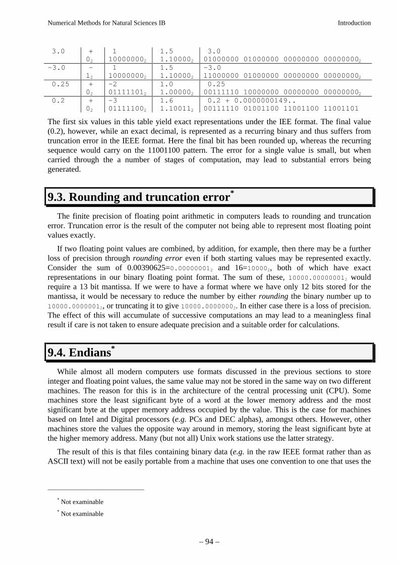
Numerical Methods for Natural Sciences IB Introduction
– 94 –
3.0 +02
1100000002
1.51.100002
3.001000000 01000000 00000000 000000002
-3.0 -12
1100000002
1.51.100002
-3.011000000 01000000 00000000 000000002
0.25 +02
-2011111012
1.01.000002
0.2500111110 10000000 00000000 000000002
0.2 +02
-3011111002
1.61.100112
0.2 + 0.0000000149..00111110 01001100 11001100 11001101
The first six values in this table yield exact representations under the IEE format. The final value(0.2), however, while an exact decimal, is represented as a recurring binary and thus suffers fromtruncation error in the IEEE format. Here the final bit has been rounded up, whereas the recurringsequence would carry on the 11001100 pattern. The error for a single value is small, but whencarried through the a number of stages of computation, may lead to substantial errors beinggenerated.
9.3. Rounding and truncation error*
The finite precision of floating point arithmetic in computers leads to rounding and truncationerror. Truncation error is the result of the computer not being able to represent most floating pointvalues exactly.
If two floating point values are combined, by addition, for example, then there may be a furtherloss of precision through rounding error even if both starting values may be represented exactly.Consider the sum of 0.00390625=0.000000012 and 16=100002, both of which have exactrepresentations in our binary floating point format. The sum of these, 10000.000000012 wouldrequire a 13 bit mantissa. If we were to have a format where we have only 12 bits stored for themantissa, it would be necessary to reduce the number by either rounding the binary number up to10000.00000012, or truncating it to give 10000.00000002. In either case there is a loss of precision.The effect of this will accumulate of successive computations an may lead to a meaningless finalresult if care is not taken to ensure adequate precision and a suitable order for calculations.
9.4. Endians*
While almost all modern computers use formats discussed in the previous sections to storeinteger and floating point values, the same value may not be stored in the same way on two differentmachines. The reason for this is in the architecture of the central processing unit (CPU). Somemachines store the least significant byte of a word at the lower memory address and the mostsignificant byte at the upper memory address occupied by the value. This is the case for machinesbased on Intel and Digital processors (e.g. PCs and DEC alphas), amongst others. However, othermachines store the values the opposite way around in memory, storing the least significant byte atthe higher memory address. Many (but not all) Unix work stations use the latter strategy.
The result of this is that files containing binary data (e.g. in the raw IEEE format rather than asASCII text) will not be easily portable from a machine that uses one convention to one that uses the
* Not examinable* Not examinable

Numerical Methods for Natural Sciences IB Introduction
– 95 –
other. A two byte integer value of 1 = 00000000 000000012 written by one machine would be readas 256 = 00000001 000000002 when read by the other machine.
Numerical Methods for Natural Sciences IB Introduction
- 96
10. Computer languages*
A complete discussion of computer languages would require a whole course initself. These notes are simply intended to give the reader a feeling for the strengthsand uses of different languages. The notes are written from the perspective ofsomeone who was brought up on a wide range of languages with programs suitable forboth procedural and object oriented approaches. The discussion is necessarily briefand may be unfairly critical on some languages.
Ideally you would use the language which is most appropriate for a givenapplication. For most projects, the language will be selected from the intersection ofthe subset of languages you know and the set of languages supported on the specificplatform you require. Only for large projects is it worth investing the time and moneyrequired to utilise the optimal language.
None of the material in this section is examinable.
10.1. Procedural verses Object Oriented*
For many applications, the current trend is towards object oriented languages suchas C++. Procedural languages are considered behind the times by many computerscientists, yet they remain the language of choice for many scientific programs. Themain procedural contender is, and has always been Fortran. Both C++ and Fortranhave their advantages, depending on the task at hand. This section is intended to act asan aid for choosing the appropriate language for a given task.
10.2. Fortran 90*
Fortran is one of the oldest languages still in wide spread use. It has long had astandard, enabling programs written for one type of machine to be relatively easilyported to run on a different type of machine, provided a Fortran compiler wasavailable. The standard has evolved to reflect changes in coding practices andrequirements. Unfortunately for many programmers, the standard lags many yearsbehind current thinking. For example, Fortran 77 is the standard to which the majorityof current compilers adhere. As the name suggests, the standard was released in 1977and the demands of computing have changed significantly since then.
The latest standard, Fortran 90, was not finally released until about 1994. Likeearlier improvements to the standard, it maintains a high level of backwardcompatibility. A Fortran 90 compiler should be able to compile all but a few of theoldest of Fortran programs (assuming they adhere to the relevant standard). WhileFortran 90 answers the majority of criticisms about the earlier version, work has
* Not examinable* Not examinable* Not examinable

Numerical Methods for Natural Sciences IB Introduction
- 97
already started on the next generation, helping to ensure Fortran remains in widespread use.
10.2.1. Procedural oriented*
The origins of Fortran as a scientific computer language are reflected in the namewhich stands for Formula Translation. The language is procedural oriented with thealgorithm (or “formula”) playing the central rôle controling the way the program iswritten and structured. In contrast, the object oriented C++ (see below) focuses on thedata. For the majority of scientific programs using the types of algorithms introducedin this course, the procedural oriented approach is more appropriate. The programgenerates data from input parameters. The underlying numerical algorithms processone type of data in a consistent manner.
As the most computationally intensive programs have traditionally followed theprocedural model, and have been written in Fortran, there has been a tremendouseffort put into developing optimisation strategies for Fortran compilers. As a result thecode produced by Fortran compilers is normally more efficient for a numericalprogram than that produced by other language compilers. In contrast, if you were todevelop a word processor, for example, in Fortran, the end result would be lessefficient (in terms of speed and size) and more cumbersome than something with thesame functionality developed in C++.
10.2.2. Fortran enhancements*
For those familiar with Fortran 77, the Fortran 90 standard has introduced many ofthe features sadly missing from the earlier version. Control structures such as DOloops have done away with the need for a numeric label. WHILE, CASE and BREAKstatements have been added to simplify program logic, and the ability to callsubroutines recursively allows the program to operate more efficiently. From the dataside structures (records), unions an maps greatly simplify the passing of parametersand the organisation of variables without resort to a multitude of COMMON blocks.
Perhaps the most significant changes accompany a move from all data structuresbeing static (i.e. the size of and space required by variables is determined at compiletime) to allowing dynamic allocation of memory. This greatly improves the flexibilityof a program and frequently allows you to achieve more with less memory as the samememory can be reused for different purposes.
Many of these enhancements have been borrowed from languages such as C++,and adapted to the Fortran environment. One of the most powerful (and, if abused,most dangerous) is the ability to overload a function or operator. By overloading afunction or operator, the precise result will depend on the type (and number) ofparameters or operands used in executing the function/operator. For example, theoperator “+” could be defined such that, when it “adds” two strings, then itconcatenates them together, perhaps stripping any trailing spaces in the process.
* Not examinable* Not examinable
Numerical Methods for Natural Sciences IB Introduction
- 98
Similarly it would be possible to define “number=string” such that the string “string”was passed to an interpreter function and the contents of it evaluated. Clearly doingsomething like defining “WRITE” as “READ” would lead to a great deal ofconfusion!
10.3. C++*
Like Fortran, C++ has evolved from earlier languages. The original, BCPL, wasadopted and enhanced by Bell Laboratories to produce B and then C as part of theirproject to develop Unix.
10.3.1. C*
The main features of C are its access to low-level features of the system and itsextremely compact (and often confusing) notation. C has often been described as awrite only language as it is relatively easy to write code which almost no one will beable to decipher. The popularity of C stems from its close association with Unix ratherthan from any inherent qualities. While there are probably still more programs writtenin Fortran and COBOL than there are in C, it is almost certain that more people useprograms written in C (or C++) than in any other language. The vast majority ofshrink wrapped applications are now written in C or C++.
While C compilers are still widely available and in common use, there is little orno justification for using C for any new project. C++ (which is more than just animproved version of C) provides all the functionality of C and allows the code to bewritten in a more flexible and readable manner.
Many programs were written in C during the late 1980s because it was the “in”language rather than the best for a given application. As a result of this investment andthe relative simplicity of gradually moving over to C++, most mainstream applicationsin C
10.3.2. Object Oriented*
As systems became bigger, it became desirable – often essential – to reusecomponents as much as possible. Historically this was achieved through the use ofsoftware libraries, but such libraries tend to be useful only for low-level routines. Theconcept of Object Oriented Programming was introduced to C to provide a straightforward way of handling many similar – but not identical – objects without having towrite specialised code for each object. An object is simply some data which describesa coherent unit.
* Not examinable* Not examinable* Not examinable
Numerical Methods for Natural Sciences IB Introduction
- 99
Suppose we have an object my_cup which belongs to some class Ccup_of_drink(say). The object my_cup will take the form of a description of the cup which mightinclude information about its colour, its texture, its use and its contents. Suppose wealso have an object my_plate and that this belongs to a class Cplate_of_food. Clearlythere is much in common between a cup and a plate. They are both crockery, althoughmy_cup will contain a drink while my_plate will contain food. To save us having todefine the crockery aspects separately for my_cup and my_plate, we shall allow themto inherit these attributes from a class Ccrockery. Tableware will, in turn, inheritattributes from other classes such as Ctableware, Ccolour and Ctexture. Thishierarchy may be expressed as
Ccup_of_drink: Ccrockery, Cdrink
Cplate_of_food: Ccrockery, Cfood
Ccrockery: Ctableware, Ccolour, Ctexture
Similarly we might have a teaspoon my_teaspoon belonging to Ccutlery whichfollows
Ccutlery: Ctableware, Ccolour
The object-oriented approach comes in if we have an object my_dishwasher. Thedishwasher will accept all objects belonging to Ctableware. The classes Ccrockeryand Ccutlery are both derived from Ctableware and so any Ccrockery or Ccutleryobject is also a Ctableware object, and can thus be washed by the my_dishwasher.Similarly as Ccup_of_drink and Cplate_of_food are derived (indirectly) fromCtableware and so can be washed by my_dishwasher.
The object my_dishwasher would simply say “wash thyself” to any object itcontains. For a Ccrockery or Ccutlery object the process of washing would beidentical, and could thus be embodied at the Ctableware level. It is not quite so simplefor the Ccup_of_drink and Cplate_of_food objects as they contain food which wouldbe destroyed by the dishwasher. Thus when my_dishwasher tries to wash theCtableware derived object my_plate, it is necessary for the Cplate_of_food class tooverride the Ctableware procedure for washing. In this example the Cplate_of_foodresponse to the dishwasher may be to declare the my_plate empty of food and thenpass the request for washing the plate down to its embedded Ccrockery class whichwill in turn pass it down to Ctableware.
10.3.3. Weaknesses*
On the surface, the class structure would appear to allow C++ to be adapted to anytype of application. In practice there are some things that are difficult to achieve in aseamless way and others which lead to relatively inefficient programming. Thisinefficiency may not matter for a wordprocessor (although users of Microsoft Wordmay not agree), but can be critical for a large scale numerical simulation.
For someone brought up on most other languages, the most obvious omission issupport for multidimensional arrays. While C++ is able to have an array of arrays, and
* Not examinable
Numerical Methods for Natural Sciences IB Introduction
- 100
so have some of the functionality of a multidimensional array, they can not be used inthe same way and the usual notation can not be employed. Further, it is easy to getconfused as to what you have an array of, especially with the cryptic notation sharedby C and C++.
C++ itself is a very small language with only a few built in functions and operators.It gains its functionality through standard and specialised libraries. While this adds tothe flexibility, it has implications on the time taken to compile a program and, moreimportantly, on the execution speed. Even with the most carefully constructedlibraries and the functions being inserted in-line (instead of being called), the fact thecompiler does not understand the functions within the library limits the degree ofoptimisation which can be achieved.
10.4. Others*
10.4.1. Ada*
Touted as the language to replace all other languages, Ada was introduced in the1980s with a substantial backing from the US military. Its acceptance was slow due toits cumbersome nature and its unsuitability for many of the computers of the period.
10.4.2. Algol*
In the late 1960s and early 1970s Algol (Algorithmic Language) looked as thoughit would become the scientific computer language. Algol forced the programmer toadopt a much more structured approach than other languages at the time and offered avast array of built-in functionality such as matrix manipulation. Ultimately it was theshear power that lead to the demise of Algol as it was unable to fit on the smaller miniand microcomputers as they were developed.
10.4.3. Basic*
Basic has developed from a design exercise in Southampton to the language whichis known by more people than any other. The name Basic (Beginners SymbolicInstruction Code) does not really represent a language, but rather a family oflanguages which appear similar in concept but will differ in almost every importantdetail. Most implementations of Basic are proprietary and some are much better thanothers. Basic was designed as an interpreted language and most implementationsfollow this heritage. The name Basic is often used for the interpreted macro languagein many modern applications, especially those from Microsoft.
* Not examinable* Not examinable* Not examinable* Not examinable
Numerical Methods for Natural Sciences IB Introduction
- 101
10.4.4. Cobol*
Cobol (Common Business Oriented Language) and Fortran are the only two earlyhigh-level languages remaining in widespread use. However, whereas Fortran hasevolved with time, Cobol is essentially the same as it was 30 years ago. It is anextremely verbose, English-like language aimed at business applications. It remains inwidespread use not because of any inherent advantages, but because of the hugeinvestment which would be required to upgrade the software to a more modernlanguage.
10.4.5. Delphi*
Developed by Borland International as a competitor for Microsoft’s Visual Basic,Delphi tries to combine the graphical development tools of Visual Basic with thestructure and consistency of Pascal and the Object Oriented approach of C++ andSmalltalk. It is being predicted that Delphi will become increasingly popular on PCs.
10.4.6. Forth*
A threaded-interpreted language. Developed to control telescopes. Uses reverse-polish notation. Extremely efficient for an interpreted language, but relatively hard toread and program.
10.4.7. Lisp*
Good for Artificial Intellegence, provided you like recursion and counting brackets.
10.4.8. Modula-2*
An improved form of Pascal. Very good, but never widely accepted.
10.4.9. Pascal*
Developed as a teaching language. The standard lacks many of the featuresessential for effective computing. Most implementations provide significantenhancements to this standard, but are often not portable. Can be used for scientificprogramming, but the compilers are often inferior to those of Fortran and C++.
* Not examinable* Not examinable* Not examinable* Not examinable* Not examinable* Not examinable

Numerical Methods for Natural Sciences IB Introduction
- 102
10.4.10. PL/1*
Introduced by IBM in the 1970s as a replacement for both Cobol and Fortran, PL/1has some of the advantages and some of the disadvantages of both languages.However, it never gained much of a following due to a combination of its proprietarynature and a requirement for very substantial mainframe resources.
10.4.11. PostScript*
Often thought of as a printer protocol, PostScript is in fact a full-fledged languagewith all the normal capabilities plus built in graphics! Like Forth, PostScript is athreaded-interpreted language which results in efficient but hard to read code. WhilePostScript can be used for general-purpose computing, it is inadvisable as it would tieup the printer for a long time! Unlike most languages in wide-spread use, PostScript isa proprietary language belonging to Adobe. There are, however, many emulations ofPostScript with suitably disguised names: GhostScript, StarScript, …
10.4.12. Prolog*
10.4.13. Smalltalk*
One of the first object-oriented programming languages. It provides a moreconsistent view than C++, but is less widely accepted.
10.4.14. Visual Basic*
This flavour of Basic was introduced by Microsoft as an easy method of writingprograms for the Windows GUI. It has been an extremely successful product, butremains relatively inefficient for computational work when compared with C++ orFortran.
* Not examinable* Not examinable* Not examinable* Not examinable* Not examinable