Astronomy and Computing 3–4 (2013) 70–78

Contents lists available at ScienceDirect

Astronomy and Computing

journal homepage: www.elsevier.com/locate/ascom

Full length article

Numerical approaches for multidimensional simulations ofstellar explosionsKe-Jung Chen a,b,∗, Alexander Heger c, Ann S. Almgren d

a Department of Astronomy & Astrophysics, University of California, Santa Cruz, CA 95064, United Statesb School of Physics and Astronomy, University of Minnesota, Minneapolis, MN 55455, United Statesc Monash Centre for Astrophysics, Monash University, Victoria 3800, Australiad Computational Research Division, Lawrence Berkeley National Lab, Berkeley, CA 94720, United States

a r t i c l e i n f o

Article history:Received 28 December 2012Accepted 27 January 2014

Keywords:Computational astrophysicsSupernovaStellar evolutionMassive stars

a b s t r a c t

We introduce numerical algorithms for initializing multidimensional simulations of stellar explosionswith 1D stellar evolution models. The initial mapping from 1D profiles onto multidimensional grids cangenerate severe numerical artifacts, one of the most severe of which is the violation of conservation lawsfor physical quantities. We introduce a numerical scheme for mapping 1D spherically-symmetric dataonto multidimensional meshes so that these physical quantities are conserved. We verify our scheme byporting a realistic 1D Lagrangian stellar profile to the newmultidimensional Eulerian hydro code CASTRO.Our results show that all important features in the profiles are reproduced on the new grid and thatconservation laws are enforced at all resolutions aftermapping.We also introduce a numerical scheme forinitializing multidimensional supernova simulations with realistic perturbations predicted by 1D stellarevolutionmodels. Instead of seeding 3D stellar profileswith randomperturbations, we imprint themwithvelocity perturbations that reproduce the Kolmogorov energy spectrum expected for highly turbulentconvective regions in stars. Ourmodels return Kolmogorov energy spectra and vortex structures like thosein turbulent flows before the modes become nonlinear. Finally, we describe approaches to determiningthe resolution for simulations required to capture fluid instabilities and nuclear burning. Our algorithmsare applicable to multidimensional simulations besides stellar explosions that range from astrophysics tocosmology.

© 2014 Elsevier B.V. All rights reserved.

1. Introduction

Multidimensional simulations shed light on how fluid instabil-ities arising in supernovae (SNe) mix ejecta (Herant and Woosley,1994; Joggerst et al., 2009, 2010; Joggerst and Whalen, 2011). Un-fortunately, computing fully self-consistent 3D stellar evolutionmodels, from their formation to collapse, for the explosion setupis still beyond the realm of contemporary computational power.One alternative is to first evolve the main sequence star in a 1Dstellar evolution code in which the equations of momentum, en-ergy and mass are solved on a spherically-symmetric grid, suchas KEPLER (Weaver et al., 1978) or MESA (Paxton et al., 2011).

∗ Corresponding author at: Department of Astronomy & Astrophysics, Universityof California, Santa Cruz, CA 95064, United States. Tel.: +1 6126242327.

E-mail addresses: chen1399@umn.edu, ken@asiaa.sinica.edu.tw,kchen@physics.umn.edu (K.-J. Chen).

http://dx.doi.org/10.1016/j.ascom.2014.01.0012213-1337/© 2014 Elsevier B.V. All rights reserved.

Once the star reaches the pre-supernova phase, its 1D profilescan then be mapped into multidimensional hydro codes such asCASTRO (Almgren et al., 2010; Zhang et al., 2011) or FLASH (Fryx-ell et al., 2000) and continue to be evolved until the starexplodes.

Differences between codes in dimensionality and coordinatemesh can lead to numerical issues such as violation of conserva-tion of mass and energy when profiles are mapped from one codeto another. A first, simple approach could be to initialize multidi-mensional grids by linear interpolation from corresponding meshpoints on the 1D profiles. However, linear interpolation becomesinvalid when the new grid fails to resolve critical features in theoriginal profile such as the inner core of a star. This is especiallytrue when porting profiles from 1D Lagrangian codes, which caneasily resolve very small spatial features in mass coordinate, to afixed or adaptive Eulerian grid. In addition to conservation laws,some physical processes such as nuclear burning are very sensi-tive to temperature, so errors inmapping can lead to very different

K.-J. Chen et al. / Astronomy and Computing 3–4 (2013) 70–78 71

outcomes for the simulations such as altering the nucleosynthesisand energetics of SNe. None address the conservation of physicalquantities by such procedures.We examine these issues and intro-duce a new scheme for mapping 1D data sets to multidimensionalgrids.

Seeding the pre-supernova profile of the star with realistic per-turbations is important to illuminate how fluid instabilities latererupt and mix the star during the explosion. Massive stars usuallydevelop convective zones prior to exploding as SNe (Woosley et al.,2002; Heger and Woosley, 2002). Multidimensional stellar evolu-tion models suggest that the fluid inside the convective regionscan be highly turbulent (Porter and Woodward, 2000; Arnett andMeakin, 2011). However, in lieu of the 3D stellar evolution calcula-tions necessary to produce such perturbations from first principles,multidimensional simulations are usually just seededwith randomperturbations. In reality, if the star is convective and the fluid inthose zones is turbulent (Davidson, 2004), a better approach is toimprint the multidimensional profiles with velocity perturbationswith a Kolmogorov energy spectrum (Frisch, 1995).

In addition to implementing realistic initial conditions, caremust be taken to determine the resolution that multidimensionalsimulations require to resolve the most important physical scalesand yield consistent results given the computational resources thatare available. We provide a systematic approach for finding thisresolution for multidimensional stellar explosions. The structureof the paper is as follows; in Section 2 we describe the key featuresof the KEPLER and CASTRO codes.We describe our initial mappingscheme and demonstrate it by porting a massive star model fromKEPLER toCASTRO in Section 3.We reviewour scheme for seeding2D and 3D stellar profileswith turbulent perturbations and presenthydrodynamic simulations done with these profiles in CASTRO inSection 4. We provide a strategy for finding the proper resolutionfor multidimensional simulations with multiscale processes suchas hydrodynamics and nuclear burning in Section 5 and concludethe results in Section 6.

2. Stellar model

We model the evolution of main sequence stars with KEPLER(Weaver et al., 1978), a 1D Lagrangian stellar evolution code.KEPLER solves the evolution equations for mass, momentum, andenergy, including relevant physical processes such as nuclear burn-ing and mixing due to convection. When the star reaches the pre-supernova phase (hundreds of seconds prior to launching the SNshock), we map its 1D profiles onto a multidimensional grid inCASTRO. When the star explodes, its initial spherical symmetry isbroken by fluid instabilities formed during the explosion that can-not bemodeled by 1D calculations. Hence, we follow the evolutionof the star in CASTRO until it explodes.

Here our thermonuclear supernovae refer to those from verymassive stars. They are totally different from the Type-Ia ex-plosions. Very massive stars with initial masses of 150–260M⊙

develop oxygen cores of &50M⊙ after central carbon burning(Barkat et al., 1967; Heger and Woosley, 2002). At this point,the core reaches sufficiently high temperatures (∼109 K) and atrelatively low densities (∼106 g cm−3) to favor the creation ofelectron–positron pairs (high-entropy hot plasma). The pressure-supporting photons turn into the rest masses for pairs and softenthe adiabatic index γ of the gas below a critical value of 4

3 , whichcauses a dynamical instability and triggers rapid contraction of thecore. During contraction, core temperatures and densities swiftlyrise, and oxygen and silicon ignite, burning rapidly. This reversesthe preceding contraction (enough entropy is generated so theequation of state leaves the regime of pair instability), and a shockforms at the outer edge of the core. This thermonuclear explosion,known as a pair-instability supernova (PSN), completely disrupts

C/O

H

He

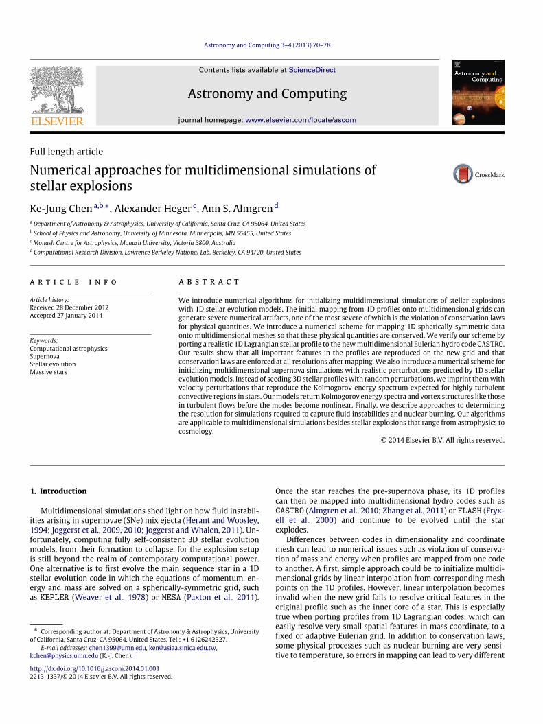
Fig. 1. After central helium burning, the helium core of very massive star becomeshighly convective (wavy mesh) and radiation energy is converted into electron andpositron pairs at its oxygen core; This results in an implosion that ignites the oxygenand silicon explosively. The energy released from burning eventually blows up thestar.

the star with explosion energies of up to 1053 erg, leaving no com-pact remnant and producing up to 50M⊙

56Ni. Fig. 1 illustrates thestellar structure of pre-psn and its explosion.

CASTRO (Almgren et al., 2010; Zhang et al., 2011) is a massivelyparallel, multidimensional Eulerian adaptive mesh refinement(AMR) radiation-hydrodynamics code for astrophysical applica-tions. Its time integration of the hydrodynamics equations is basedon a higher-order, unsplit Godunov scheme. Block-structured AMRwith subcycling in time applies high spatial resolution to where itis needed most. We use the Helmholtz equation of state (Timmesand Swesty, 2000)with density, temperature, and elemental abun-dances; it includes contributions by non-degenerate and degen-erate relativistic and non-relativistic electrons, electron–positronpair production, ions and radiation. The gravitational field iscalculated with a monopole approximation derived from a radialaverage of the density on the multidimensional grid. We have im-plemented several reaction networks (7, 13, 19 isotopes) (Weaveret al., 1978; Timmes, 1999) in CASTRO for calculating nucleosyn-thesis and energetics in thermonuclear SNe. Themost comprehen-sive network includes alpha-chain reactions, heavy-ion reactions,hydrogen burning cycles, photo-disintegration of heavy elements,and energy loss by neutrinos.

3. Conservative mapping

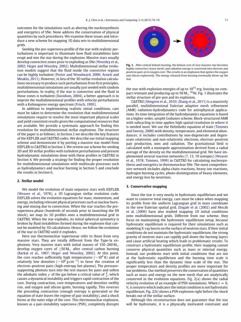
Since the star is very nearly in hydrostatic equilibrium and wewant to conserve total energy, care must be taken when mappingits profile from the uniform Lagrangian grid in mass coordinateto the new Eulerian spatial grid. Zingale et al. (2002) and Mocáket al. (2009) have also studied mapping 1D initial conditionsonto multidimensional grids. Different from our scheme, theyfocus on maintaining the hydrostatic equilibrium setup, becausehydrostatic equilibrium is required for their simulations such asmodeling X-ray bursts on the surface of neutron stars. If their initialconditions do not maintain the hydrostatic equilibrium, the stronggravity of neutron stars can rapidly pull down the burning layersand cause artificial heating which leads to problematic results. Toconstruct a hydrostatic equilibrium profile, their mapping cannotconserve physical quantities such as mass or internal energy.Instead, our problems start with initial conditions that are notat the hydrostatic equilibrium and the burning time scale issignificantly less than the dynamic time scale of the star. Theproper temperature and density profiles are more important forour problems. Ourmethodpreserves the conservation of quantitiessuch as mass and energy on the new mesh that are analyticallyconserved in the evolution equations. Fig. 2(a) shows the radialvelocity evolution of an example of PSN simulations. When t = 0,Vr is nonzerowhich indicates the initial condition is not hydrostaticequilibrium. Fig. 2(b) shows a PSN explosion right before the shockbreaks out of the stellar surface.

Although this reconstruction does not guarantee that the starwill be hydrostatic, it is a physically motivated constraint and

72 K.-J. Chen et al. / Astronomy and Computing 3–4 (2013) 70–78

(a) Evolution of radial velocity profiles. (b) A PSN explosion.

Fig. 2. (a) The in-falling velocities of collapsing core begin at about 200 km s−1 . After the explosion occurs, a strong shock is launched and will propagate until it breaks outfrom the stellar surface. (b) The fluid instabilities generated during the explosion evolve into a large spatial scale and generated a significant mixing.

sufficient for our simulations. The algorithmwe describe is specificto our models but can be easily generalized to mappings of other1D data to higher dimensional grids.

3.1. Method

First, we construct a continuous (C0) function that conserves thephysical quantity uponmapping onto the new grid. An ideal choicefor interpolation is the volume coordinate V , the volume enclosedby a given radius from the center of the star. Then, integrating adensity ρX (which can represent mass or internal energy density)with respect to the volume coordinate yields a conserved quantityX

X =

V2

V1ρX dV , (1)

such as the total mass or total internal energy lying in the shellbetween V1 and V2.

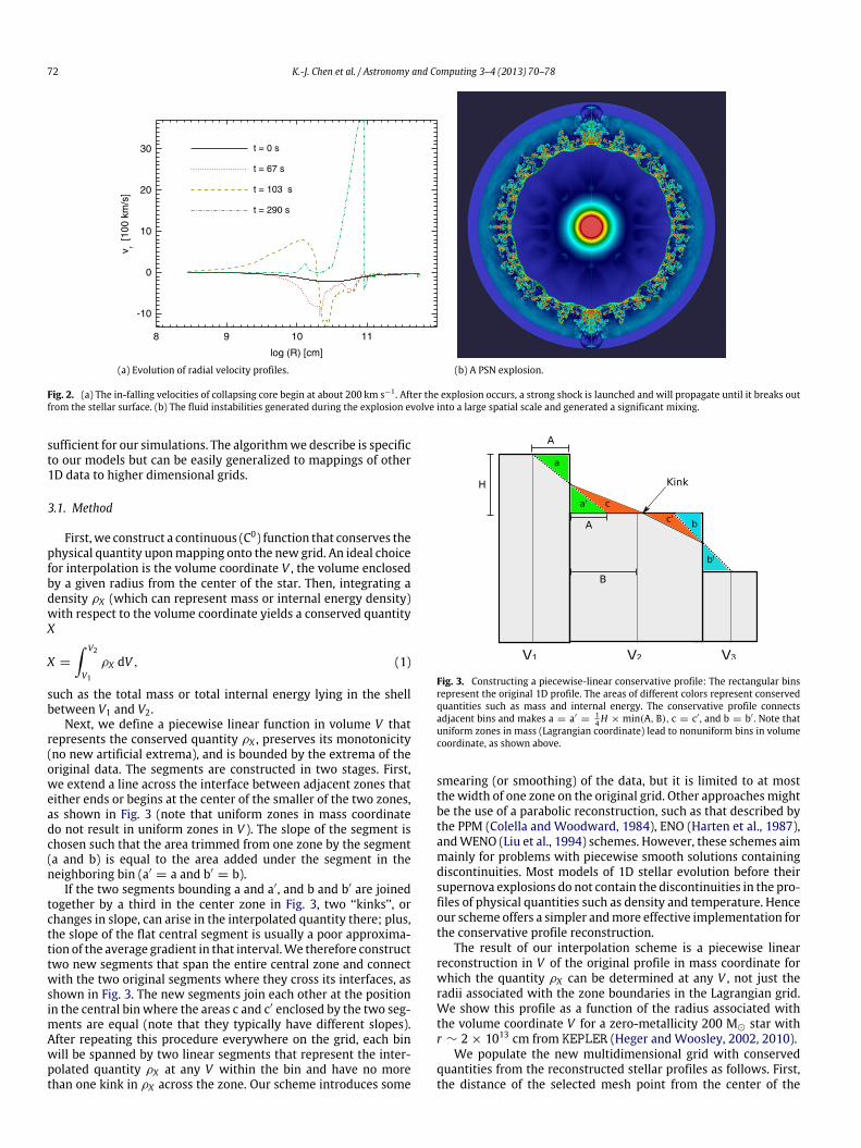
Next, we define a piecewise linear function in volume V thatrepresents the conserved quantity ρX , preserves its monotonicity(no new artificial extrema), and is bounded by the extrema of theoriginal data. The segments are constructed in two stages. First,we extend a line across the interface between adjacent zones thateither ends or begins at the center of the smaller of the two zones,as shown in Fig. 3 (note that uniform zones in mass coordinatedo not result in uniform zones in V ). The slope of the segment ischosen such that the area trimmed from one zone by the segment(a and b) is equal to the area added under the segment in theneighboring bin (a′

= a and b′= b).

If the two segments bounding a and a′, and b and b′ are joinedtogether by a third in the center zone in Fig. 3, two ‘‘kinks’’, orchanges in slope, can arise in the interpolated quantity there; plus,the slope of the flat central segment is usually a poor approxima-tion of the average gradient in that interval.We therefore constructtwo new segments that span the entire central zone and connectwith the two original segments where they cross its interfaces, asshown in Fig. 3. The new segments join each other at the positionin the central bin where the areas c and c′ enclosed by the two seg-ments are equal (note that they typically have different slopes).After repeating this procedure everywhere on the grid, each binwill be spanned by two linear segments that represent the inter-polated quantity ρX at any V within the bin and have no morethan one kink in ρX across the zone. Our scheme introduces some

Fig. 3. Constructing a piecewise-linear conservative profile: The rectangular binsrepresent the original 1D profile. The areas of different colors represent conservedquantities such as mass and internal energy. The conservative profile connectsadjacent bins and makes a = a′

=14H × min(A, B), c = c′ , and b = b′ . Note that

uniform zones in mass (Lagrangian coordinate) lead to nonuniform bins in volumecoordinate, as shown above.

smearing (or smoothing) of the data, but it is limited to at mostthe width of one zone on the original grid. Other approachesmightbe the use of a parabolic reconstruction, such as that described bythe PPM (Colella and Woodward, 1984), ENO (Harten et al., 1987),andWENO (Liu et al., 1994) schemes. However, these schemes aimmainly for problems with piecewise smooth solutions containingdiscontinuities. Most models of 1D stellar evolution before theirsupernova explosions do not contain the discontinuities in the pro-files of physical quantities such as density and temperature. Henceour scheme offers a simpler andmore effective implementation forthe conservative profile reconstruction.

The result of our interpolation scheme is a piecewise linearreconstruction in V of the original profile in mass coordinate forwhich the quantity ρX can be determined at any V , not just theradii associated with the zone boundaries in the Lagrangian grid.We show this profile as a function of the radius associated withthe volume coordinate V for a zero-metallicity 200 M⊙ star withr ∼ 2 × 1013 cm from KEPLER (Heger and Woosley, 2002, 2010).

We populate the new multidimensional grid with conservedquantities from the reconstructed stellar profiles as follows. First,the distance of the selected mesh point from the center of the

K.-J. Chen et al. / Astronomy and Computing 3–4 (2013) 70–78 73

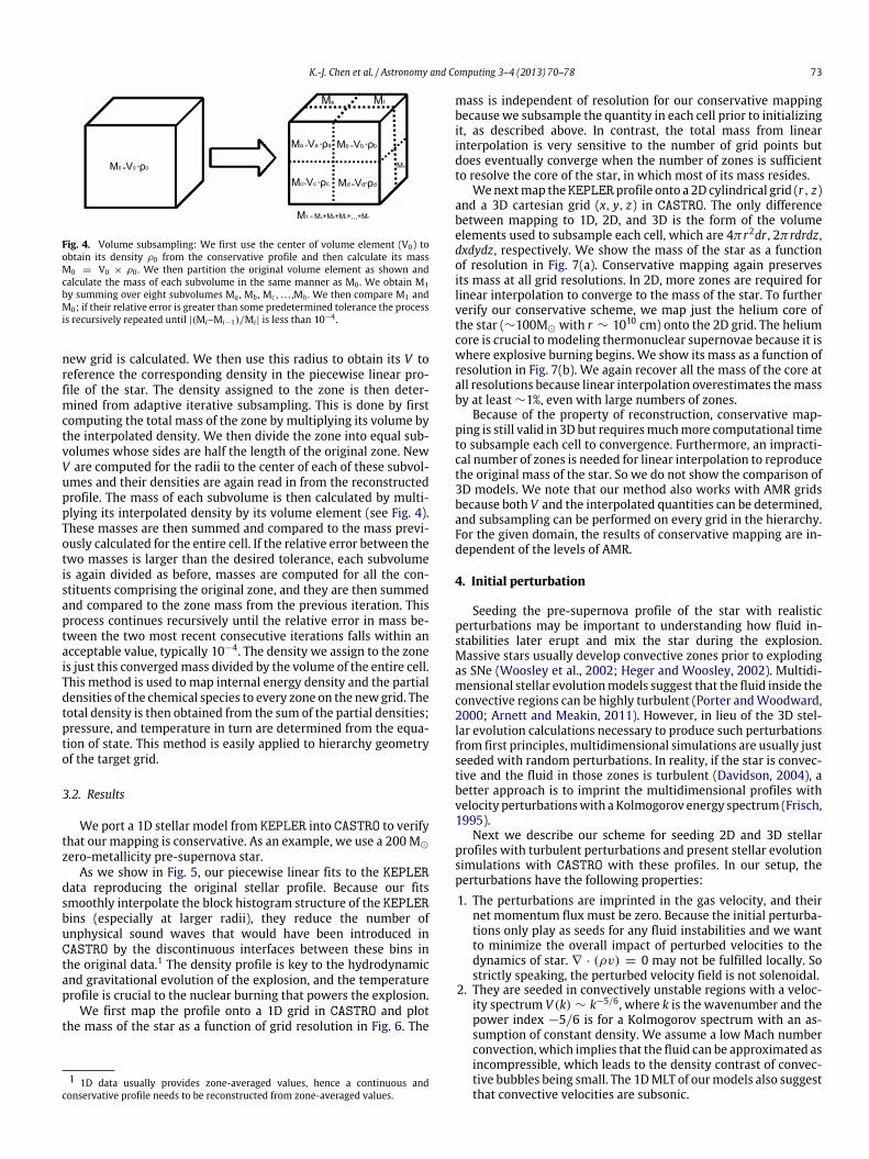
Fig. 4. Volume subsampling: We first use the center of volume element (V0) toobtain its density ρ0 from the conservative profile and then calculate its massM0 = V0 × ρ0 . We then partition the original volume element as shown andcalculate the mass of each subvolume in the same manner as M0 . We obtain M1by summing over eight subvolumes Ma , Mb , Mc , . . . ,Mh . We then compare M1 andM0; if their relative error is greater than some predetermined tolerance the processis recursively repeated until |(Mi–Mi−1)/Mi| is less than 10−4 .

new grid is calculated. We then use this radius to obtain its V toreference the corresponding density in the piecewise linear pro-file of the star. The density assigned to the zone is then deter-mined from adaptive iterative subsampling. This is done by firstcomputing the total mass of the zone by multiplying its volume bythe interpolated density. We then divide the zone into equal sub-volumes whose sides are half the length of the original zone. NewV are computed for the radii to the center of each of these subvol-umes and their densities are again read in from the reconstructedprofile. The mass of each subvolume is then calculated by multi-plying its interpolated density by its volume element (see Fig. 4).These masses are then summed and compared to the mass previ-ously calculated for the entire cell. If the relative error between thetwo masses is larger than the desired tolerance, each subvolumeis again divided as before, masses are computed for all the con-stituents comprising the original zone, and they are then summedand compared to the zone mass from the previous iteration. Thisprocess continues recursively until the relative error in mass be-tween the two most recent consecutive iterations falls within anacceptable value, typically 10−4. The density we assign to the zoneis just this convergedmass divided by the volume of the entire cell.This method is used to map internal energy density and the partialdensities of the chemical species to every zone on the newgrid. Thetotal density is then obtained from the sum of the partial densities;pressure, and temperature in turn are determined from the equa-tion of state. This method is easily applied to hierarchy geometryof the target grid.

3.2. Results

We port a 1D stellar model from KEPLER into CASTRO to verifythat our mapping is conservative. As an example, we use a 200M⊙

zero-metallicity pre-supernova star.As we show in Fig. 5, our piecewise linear fits to the KEPLER

data reproducing the original stellar profile. Because our fitssmoothly interpolate the block histogram structure of the KEPLERbins (especially at larger radii), they reduce the number ofunphysical sound waves that would have been introduced inCASTRO by the discontinuous interfaces between these bins inthe original data.1 The density profile is key to the hydrodynamicand gravitational evolution of the explosion, and the temperatureprofile is crucial to the nuclear burning that powers the explosion.

We first map the profile onto a 1D grid in CASTRO and plotthe mass of the star as a function of grid resolution in Fig. 6. The

1 1D data usually provides zone-averaged values, hence a continuous andconservative profile needs to be reconstructed from zone-averaged values.

mass is independent of resolution for our conservative mappingbecause we subsample the quantity in each cell prior to initializingit, as described above. In contrast, the total mass from linearinterpolation is very sensitive to the number of grid points butdoes eventually converge when the number of zones is sufficientto resolve the core of the star, in which most of its mass resides.

Wenextmap theKEPLERprofile onto a 2D cylindrical grid (r, z)and a 3D cartesian grid (x, y, z) in CASTRO. The only differencebetween mapping to 1D, 2D, and 3D is the form of the volumeelements used to subsample each cell, which are 4πr2dr , 2πrdrdz,dxdydz, respectively. We show the mass of the star as a functionof resolution in Fig. 7(a). Conservative mapping again preservesits mass at all grid resolutions. In 2D, more zones are required forlinear interpolation to converge to the mass of the star. To furtherverify our conservative scheme, we map just the helium core ofthe star (∼100M⊙ with r ∼ 1010 cm) onto the 2D grid. The heliumcore is crucial to modeling thermonuclear supernovae because it iswhere explosive burning begins. We show its mass as a function ofresolution in Fig. 7(b). We again recover all the mass of the core atall resolutions because linear interpolation overestimates themassby at least ∼1%, even with large numbers of zones.

Because of the property of reconstruction, conservative map-ping is still valid in 3D but requiresmuchmore computational timeto subsample each cell to convergence. Furthermore, an impracti-cal number of zones is needed for linear interpolation to reproducethe original mass of the star. So we do not show the comparison of3D models. We note that our method also works with AMR gridsbecause both V and the interpolated quantities can be determined,and subsampling can be performed on every grid in the hierarchy.For the given domain, the results of conservative mapping are in-dependent of the levels of AMR.

4. Initial perturbation

Seeding the pre-supernova profile of the star with realisticperturbations may be important to understanding how fluid in-stabilities later erupt and mix the star during the explosion.Massive stars usually develop convective zones prior to explodingas SNe (Woosley et al., 2002; Heger and Woosley, 2002). Multidi-mensional stellar evolutionmodels suggest that the fluid inside theconvective regions can be highly turbulent (Porter andWoodward,2000; Arnett and Meakin, 2011). However, in lieu of the 3D stel-lar evolution calculations necessary to produce such perturbationsfrom first principles,multidimensional simulations are usually justseeded with random perturbations. In reality, if the star is convec-tive and the fluid in those zones is turbulent (Davidson, 2004), abetter approach is to imprint the multidimensional profiles withvelocity perturbationswith aKolmogorov energy spectrum (Frisch,1995).

Next we describe our scheme for seeding 2D and 3D stellarprofiles with turbulent perturbations and present stellar evolutionsimulations with CASTRO with these profiles. In our setup, theperturbations have the following properties:1. The perturbations are imprinted in the gas velocity, and their

net momentum flux must be zero. Because the initial perturba-tions only play as seeds for any fluid instabilities and we wantto minimize the overall impact of perturbed velocities to thedynamics of star. ∇ · (ρv) = 0 may not be fulfilled locally. Sostrictly speaking, the perturbed velocity field is not solenoidal.

2. They are seeded in convectively unstable regions with a veloc-ity spectrum V (k) ∼ k−5/6, where k is the wavenumber and thepower index −5/6 is for a Kolmogorov spectrum with an as-sumption of constant density. We assume a low Mach numberconvection,which implies that the fluid can be approximated asincompressible, which leads to the density contrast of convec-tive bubbles being small. The 1DMLT of ourmodels also suggestthat convective velocities are subsonic.

74 K.-J. Chen et al. / Astronomy and Computing 3–4 (2013) 70–78

(a) Inner density profile. (b) Inner temperature profile.

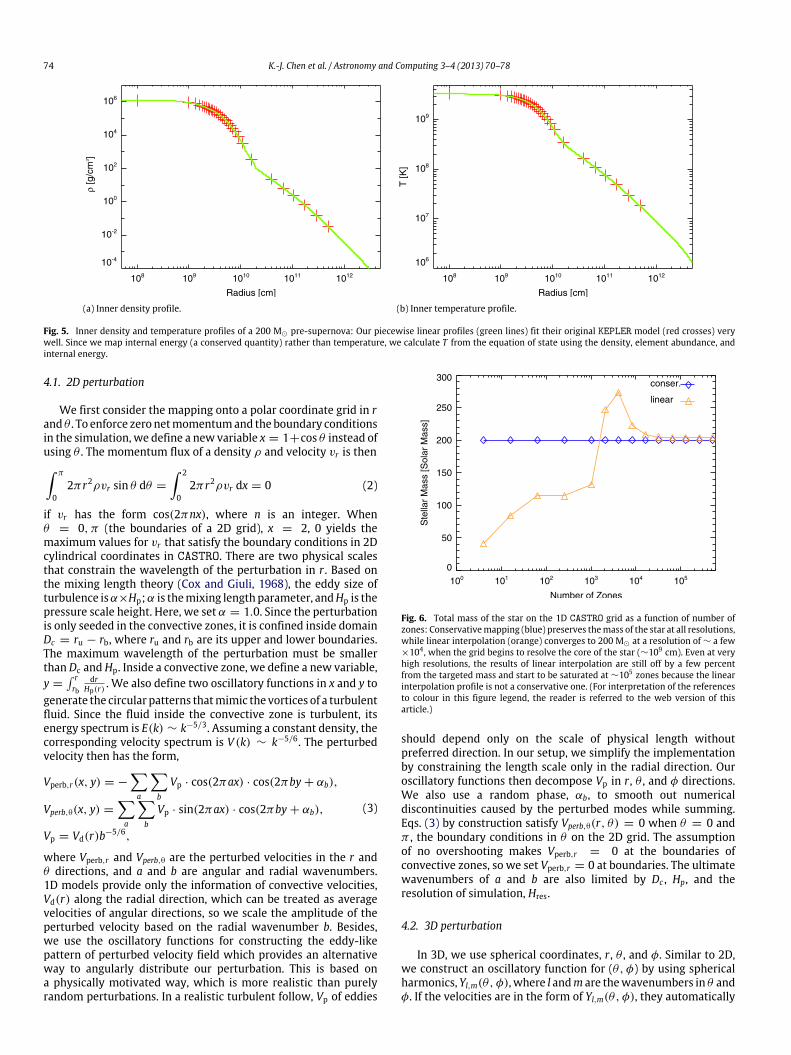
Fig. 5. Inner density and temperature profiles of a 200 M⊙ pre-supernova: Our piecewise linear profiles (green lines) fit their original KEPLER model (red crosses) verywell. Since we map internal energy (a conserved quantity) rather than temperature, we calculate T from the equation of state using the density, element abundance, andinternal energy.

4.1. 2D perturbation

We first consider the mapping onto a polar coordinate grid in rand θ . To enforce zero netmomentumand the boundary conditionsin the simulation, we define a new variable x = 1+cos θ instead ofusing θ . The momentum flux of a density ρ and velocity vr is then π

02πr2ρvr sin θ dθ =

2

02πr2ρvr dx = 0 (2)

if vr has the form cos(2πnx), where n is an integer. Whenθ = 0, π (the boundaries of a 2D grid), x = 2, 0 yields themaximum values for vr that satisfy the boundary conditions in 2Dcylindrical coordinates in CASTRO. There are two physical scalesthat constrain the wavelength of the perturbation in r . Based onthe mixing length theory (Cox and Giuli, 1968), the eddy size ofturbulence isα×Hp;α is themixing lengthparameter, andHp is thepressure scale height. Here, we set α = 1.0. Since the perturbationis only seeded in the convective zones, it is confined inside domainDc = ru − rb, where ru and rb are its upper and lower boundaries.The maximum wavelength of the perturbation must be smallerthan Dc andHp. Inside a convective zone, we define a new variable,y =

rrb

drHp(r) . We also define two oscillatory functions in x and y to

generate the circular patterns thatmimic the vortices of a turbulentfluid. Since the fluid inside the convective zone is turbulent, itsenergy spectrum is E(k) ∼ k−5/3. Assuming a constant density, thecorresponding velocity spectrum is V (k) ∼ k−5/6. The perturbedvelocity then has the form,

Vperb,r(x, y) = −

a

b

Vp · cos(2πax) · cos(2πby + αb),

Vperb,θ(x, y) =

a

b

Vp · sin(2πax) · cos(2πby + αb),

Vp = Vd(r)b−5/6,

(3)

where Vperb,r and Vperb,θ are the perturbed velocities in the r andθ directions, and a and b are angular and radial wavenumbers.1D models provide only the information of convective velocities,Vd(r) along the radial direction, which can be treated as averagevelocities of angular directions, so we scale the amplitude of theperturbed velocity based on the radial wavenumber b. Besides,we use the oscillatory functions for constructing the eddy-likepattern of perturbed velocity field which provides an alternativeway to angularly distribute our perturbation. This is based ona physically motivated way, which is more realistic than purelyrandom perturbations. In a realistic turbulent follow, Vp of eddies

Fig. 6. Total mass of the star on the 1D CASTRO grid as a function of number ofzones: Conservativemapping (blue) preserves themass of the star at all resolutions,while linear interpolation (orange) converges to 200 M⊙ at a resolution of ∼ a few×104 , when the grid begins to resolve the core of the star (∼109 cm). Even at veryhigh resolutions, the results of linear interpolation are still off by a few percentfrom the targeted mass and start to be saturated at ∼105 zones because the linearinterpolation profile is not a conservative one. (For interpretation of the referencesto colour in this figure legend, the reader is referred to the web version of thisarticle.)

should depend only on the scale of physical length withoutpreferred direction. In our setup, we simplify the implementationby constraining the length scale only in the radial direction. Ouroscillatory functions then decompose Vp in r , θ , and φ directions.We also use a random phase, αb, to smooth out numericaldiscontinuities caused by the perturbed modes while summing.Eqs. (3) by construction satisfy Vperb,θ(r, θ) = 0 when θ = 0 andπ , the boundary conditions in θ on the 2D grid. The assumptionof no overshooting makes Vperb,r = 0 at the boundaries ofconvective zones, so we set Vperb,r = 0 at boundaries. The ultimatewavenumbers of a and b are also limited by Dc , Hp, and theresolution of simulation, Hres.

4.2. 3D perturbation

In 3D, we use spherical coordinates, r , θ , and φ. Similar to 2D,we construct an oscillatory function for (θ, φ) by using sphericalharmonics, Yl,m(θ, φ), where l andm are thewavenumbers in θ andφ. If the velocities are in the form of Yl,m(θ, φ), they automatically

K.-J. Chen et al. / Astronomy and Computing 3–4 (2013) 70–78 75

(a) 2D mapped mass of entire star. (b) 2D mapped mass of helium core.

Fig. 7. (a) Total mass of the star on the new 2D CASTRO grid as a function of number of zones in both r and z: Conservative mapping (blue) recovers the mass of the starat all resolutions and linear interpolation (orange) approaches 200 M⊙ at a resolution of ∼20482 . (b) Total mass of the He core on the 2D CASTRO grid as a function ofnumber of zones in both r and z: Conservative mapping (blue) preserves its original mass at all resolutions while linear interpolation (orange) begins to converge to 100M⊙ at a resolution of 642 , but it is still off by ∼1% even as the resolution approaches ∼20482 because the linear interpolation profile is, by nature, not conservative. (Forinterpretation of the references to colour in this figure legend, the reader is referred to the web version of this article.)

conservemomentum fluxwhile summing all themodes l,m. In theradial direction, we use cos(cy), where c is the wavenumber in theradial direction and y is as defined in 2D. The perturbation then hasthe following form:

Vperb,x(r, θ, φ) = Vperb sin(θ) cos(φ),Vperb,y(r, θ, φ) = Vperb sin(θ) sin(φ),Vperb,z(r, θ, φ) = Vperb cos(θ),

Vperb =

c

l

m

Vp · Yl,m(θ + ωlm, φ + ωlm)

· cos(2πcy + λc),

Vp = Vd(r)c−5/6,

(4)

where Vperb,x, Vperb,y, Vperb,z are the perturbed velocities in the x,y, and z directions. We sum over the modes, applying randomphases ωlm and λc to smooth out numerical discontinuities causedby different perturbed modes. Similar to 2D, Vp is only scaled byradial wavenumber c. Because there are no reflective boundaryconditions for 3D, we only take care of the boundary conditions inradial direction.We again assume there is no overshooting outsidethe boundaries of convective zones, so we enforce Vperb to zero atboundaries.

4.3. Results

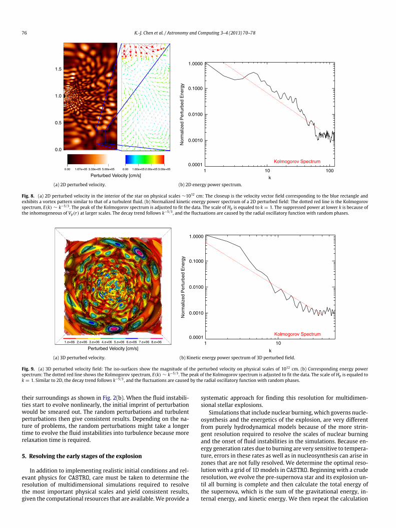
We first initialize perturbations on a 2D grid with a profilethat is derived from a 1D KEPLER stellar evolution calculation.The perturbations are confined to regions that are convectivelyunstable (Heger et al., 2000). Themagnitude Vd(r) of the perturbedvelocity adopts the diffusion velocity, which is usually ∼1%–10%of the local sound speed. We again consider a zero-metallicity200M⊙ star in the pre-supernova phase. This star develops alarge convection zone that extends out to the hydrogen envelope.We show the magnitude of the perturbed velocity generated bythe two oscillatory functions discussed above on our 2D gridin Fig. 8(a). The velocity field satisfies the reflecting boundaryconditions on the 2D grid at θ = 0 and π . In the right panel weshow velocity vectors in the selected subregion on the left (bluerectangle). A clear vortex pattern that mimics a turbulent fluid isclearly visible. Next we calculate energy spectrum of perturbedvelocity field. We first randomly pick a radial direction (constantθ in 2D) or (constant θ and φ) in 3D) inside the convective zone,perform Fourier transfer of Vp along the radial direction, then

calculate its power spectrum. We repeat the same process tentimes, our final spectrum is obtained by averaging all spectrapreviously calculated. k = Hp/l, where Hp is the pressure scaleheight and l is the physical scale in r direction. Fig. 8(b) showsthe energy spectrum of the fluid, which is basically a Kolmogorovspectrum E(k) ∼ k−5/3 except for fluctuations in part causedby the random phases in the sum over modes in r , and Vd(r)is not a constant across the convective region that produces anoffset in the smaller k region. The energies would converge to theKolmogorov spectrum in the limit of large k, but the maximum kof our simulation is limited to the resolution of the grid.

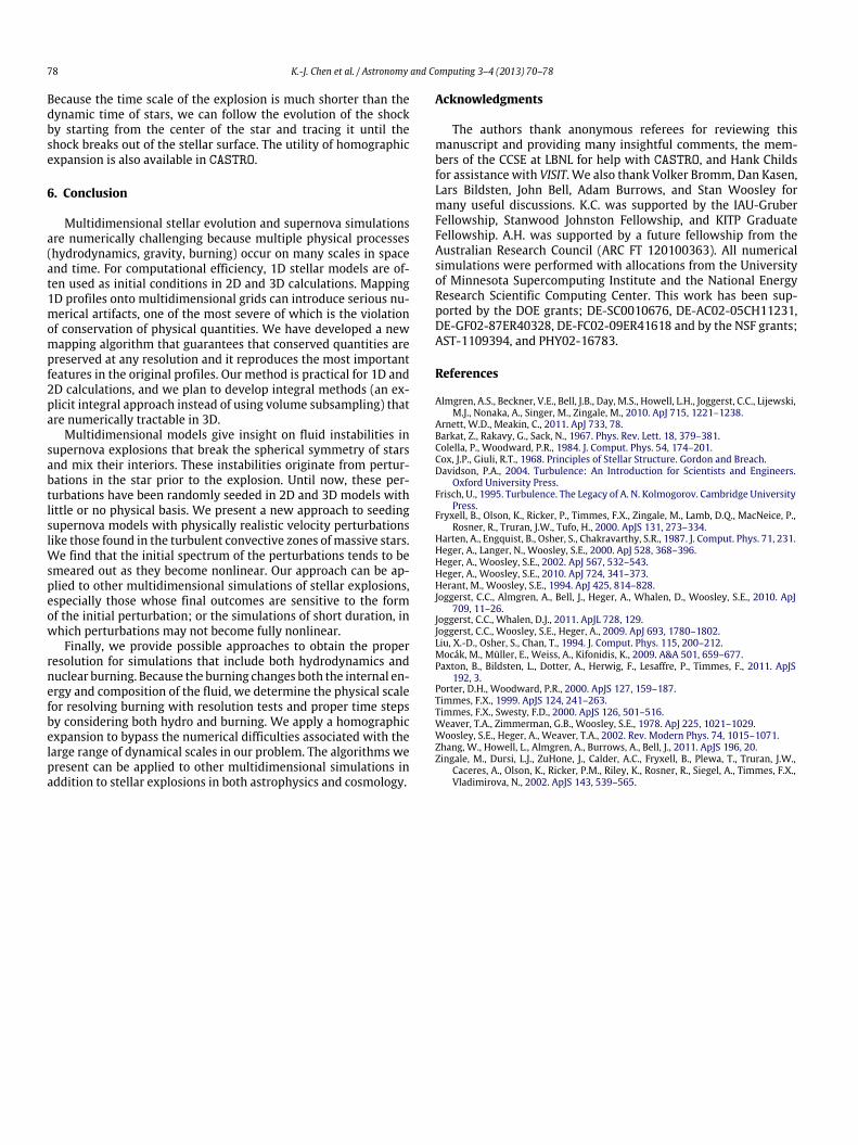
We next port our 1D KEPLER model to a 3D grid. In Fig. 9(a),we show a slice of the magnitude of the perturbed velocity, whichagain exhibits the clear cell pattern reminiscent of the vorticesof a turbulent fluid. The velocity pattern in 3D is more irregularthan in 2D. We show the energy spectrum of the velocity fieldin Fig. 9(b), which is similar to that of our 2D spectrum but withlarger fluctuations that are again due to the random phases weassign to each spherical harmonic, and the Vd(r) is not a constantacross the convective region that produces an offset in the smallerk region. We also check the values of perturbed velocities whetherthey are consistent to the Vd(r) or not. We calculate the standarddeviation of radial velocities; δVr =

⟨(V (r) − ⟨V (r)⟩)2⟩. Fig. 10

shows the comparison between δVr and Vd as a function of radius.The values of δVr are consistent to the original Vd. The oscillatorypattern of δVr comes from our formalism Eqs. (4). Above examplesdemonstrate that our scheme effectively generates turbulent fluidperturbations analog to those found in the convective regions ofmassive stars, with the desired velocity patterns and energy powerspectra.

We do not claim the models here can fully reproduce the trueturbulence found in simulations or laboratories. Unlike previousmultidimensional simulations of this kind, whose initial perturba-tions were seeded by numerical noises or random perturbations.The scheme here is the first attempt to model the initial perturba-tions based on amore realistic setup,where the convective zones ofa star play an ideal role for generating perturbations. These kineticenergy of these perturbations is very small compared with the in-ternal energy of the gas, thus it does not interfere with the over-all dynamics of the simulations or trigger an artificial ignition. Weseed initial perturbations to trigger the fluid instabilities on mul-tidimensional simulations so we can study how they evolve with

76 K.-J. Chen et al. / Astronomy and Computing 3–4 (2013) 70–78

1.5

1.0

0.5

0.0

0.00 1.67e+05 3.33e+05 5.00e+05 0.00 1.00e+05 2.00e+05 3.00e+05

Perturbed Velocity [cm/s]

(a) 2D perturbed velocity. (b) 2D energy power spectrum.

Fig. 8. (a) 2D perturbed velocity in the interior of the star on physical scales ∼1012 cm: The closeup is the velocity vector field corresponding to the blue rectangle andexhibits a vortex pattern similar to that of a turbulent fluid. (b) Normalized kinetic energy power spectrum of a 2D perturbed field: The dotted red line is the Kolmogorovspectrum, E(k) ∼ k−5/3 . The peak of the Kolmogorov spectrum is adjusted to fit the data. The scale of Hp is equaled to k = 1. The suppressed power at lower k is because ofthe inhomogeneous of Vp(r) at larger scales. The decay trend follows k−5/3 , and the fluctuations are caused by the radial oscillatory function with random phases.

2.e+06 3.e+06 4.e+06 5.e+06 6.e+06 7.e+06

Perturbed Velocity [cm/s]

1.e+06 8.e+06

(a) 3D perturbed velocity. (b) Kinetic energy power spectrum of 3D perturbed field.

Fig. 9. (a) 3D perturbed velocity field: The iso-surfaces show the magnitude of the perturbed velocity on physical scales of 1012 cm. (b) Corresponding energy powerspectrum: The dotted red line shows the Kolmogorov spectrum, E(k) ∼ k−5/3 . The peak of the Kolmogorov spectrum is adjusted to fit the data. The scale of Hp is equaled tok = 1. Similar to 2D, the decay trend follows k−5/3 , and the fluctuations are caused by the radial oscillatory function with random phases.

their surroundings as shown in Fig. 2(b). When the fluid instabili-ties start to evolve nonlinearly, the initial imprint of perturbationwould be smeared out. The random perturbations and turbulentperturbations then give consistent results. Depending on the na-ture of problems, the random perturbations might take a longertime to evolve the fluid instabilities into turbulence because morerelaxation time is required.

5. Resolving the early stages of the explosion

In addition to implementing realistic initial conditions and rel-evant physics for CASTRO, care must be taken to determine theresolution of multidimensional simulations required to resolvethe most important physical scales and yield consistent results,given the computational resources that are available.We provide a

systematic approach for finding this resolution for multidimen-sional stellar explosions.

Simulations that include nuclear burning, which governs nucle-osynthesis and the energetics of the explosion, are very differentfrom purely hydrodynamical models because of the more strin-gent resolution required to resolve the scales of nuclear burningand the onset of fluid instabilities in the simulations. Because en-ergy generation rates due to burning are very sensitive to tempera-ture, errors in these rates as well as in nucleosynthesis can arise inzones that are not fully resolved. We determine the optimal reso-lution with a grid of 1Dmodels in CASTRO. Beginning with a cruderesolution, we evolve the pre-supernova star and its explosion un-til all burning is complete and then calculate the total energy ofthe supernova, which is the sum of the gravitational energy, in-ternal energy, and kinetic energy. We then repeat the calculation

K.-J. Chen et al. / Astronomy and Computing 3–4 (2013) 70–78 77

Fig. 10. δVr and Vd as a function r inside the convective zone of the star: The valuesof δVr inside the convective zone are about 106 cm s−1 , those are consistent to thevalues of Vd , predicted from the 1DMLT theory. The oscillatory trend of δVr reflectsthe original function form of the perturbations.

with the same setup but with a finer resolution and again calculatethe total energy of the explosion. We repeat this process until thetotal energy is converged. As shown in Fig. 11, our example of a200M⊙ pre-supernova converges when the resolution of the gridapproaches 108 cm.

The time scales of burning (dtb) and hydrodynamics (dth) canbe very disparate, so we adopt time steps of min(dth, dtb) in oursimulations, where dth =

dxcs+|v|

; dx is the grid resolution, cs is thelocal sound speed, v is the fluid velocity, and the time scale forburning is dtb, which is determined by both the energy generationrate and the rate of change of the abundances.

5.1. Homographic expansion

Aswehave shown, grid resolutions of 108 cmare needed to fullyresolve nuclear burning in our model. However, the star can havea radius of up to several 1014 cm. This large dynamical range (106)makes it impractical to simulate the entire star at once while fullyresolving all relevant physical processes.When the shock launchesfrom the center of the star, the shock’s traveling time scale is abouta few days, which is much shorter than the Kelvin–Helmholtz timescale of the stars, about several million years. We can assume that

Fig. 12. Homographic expansion: In both panels, the yellow circle is the SN shockand the red region is the ejecta. The simulations beginwith just the inner part of thestar and a higher resolution (left panel) for capturing fluid instabilities and burning.After the explosion occurs, we follow the shock until it reaches the boundary of thesimulation box. We then expand the simulation domain, mapping the final state ofthe previous calculation onto the new mesh with a new ambient medium that istaken from the initial profile. (For interpretation of the references to colour in thisfigure legend, the reader is referred to the web version of this article.)

when the shock propagates inside the star, the stellar evolutionof the outer envelope is frozen. This allows us to trace the shockpropagation without considering the overall stellar evolution.Hence, we instead begin our simulations with a coordinate meshthat encloses just the core of the star with zones that are fineenough to resolve explosive burning. We then halt the simulationas the SN shock approaches the grid boundaries, uniformly expandthe simulation domain, and then restart the calculation. In eachexpansion we retain the same number of grids (see Fig. 12).Although the resolution decreases after each expansion, it doesnot affect the results at later times because burning is completebefore the first expansion and emergent fluid instabilities arewell resolved in later expansions. These uniform expansions arerepeated until the fluid instabilities cease to evolve. There mightbe some possible sound waves generated from boundaries undersuch a setup. However, the normal SN shocks have a much higherMach number—above 10—while traveling inside the star. Thesound waves could not contaminate the burning/fluid instabilitiesdomains before the shock reaches the boundary of the simulationbox.

Most stellar explosion problems need to deal with a largedynamic scale such as the case discussed here. It is computationallyinefficient to simulate the entire star with a sufficient resolution.

Fig. 11. Total explosion energy as a function of resolution: the x-axis is the grid resolution and the y-axis is the total energy, defined to be the sum of the gravitationalenergy, the internal energy, and the kinetic energy. The total energy is converged when the resolved scale is close to 108 cm. The right panel shows the zoom-in of the redbox in left panel. (For interpretation of the references to colour in this figure legend, the reader is referred to the web version of this article.)

78 K.-J. Chen et al. / Astronomy and Computing 3–4 (2013) 70–78

Because the time scale of the explosion is much shorter than thedynamic time of stars, we can follow the evolution of the shockby starting from the center of the star and tracing it until theshock breaks out of the stellar surface. The utility of homographicexpansion is also available in CASTRO.

6. Conclusion

Multidimensional stellar evolution and supernova simulationsare numerically challenging because multiple physical processes(hydrodynamics, gravity, burning) occur on many scales in spaceand time. For computational efficiency, 1D stellar models are of-ten used as initial conditions in 2D and 3D calculations. Mapping1D profiles onto multidimensional grids can introduce serious nu-merical artifacts, one of the most severe of which is the violationof conservation of physical quantities. We have developed a newmapping algorithm that guarantees that conserved quantities arepreserved at any resolution and it reproduces the most importantfeatures in the original profiles. Our method is practical for 1D and2D calculations, and we plan to develop integral methods (an ex-plicit integral approach instead of using volume subsampling) thatare numerically tractable in 3D.

Multidimensional models give insight on fluid instabilities insupernova explosions that break the spherical symmetry of starsand mix their interiors. These instabilities originate from pertur-bations in the star prior to the explosion. Until now, these per-turbations have been randomly seeded in 2D and 3D models withlittle or no physical basis. We present a new approach to seedingsupernova models with physically realistic velocity perturbationslike those found in the turbulent convective zones ofmassive stars.We find that the initial spectrum of the perturbations tends to besmeared out as they become nonlinear. Our approach can be ap-plied to other multidimensional simulations of stellar explosions,especially those whose final outcomes are sensitive to the formof the initial perturbation; or the simulations of short duration, inwhich perturbations may not become fully nonlinear.

Finally, we provide possible approaches to obtain the properresolution for simulations that include both hydrodynamics andnuclear burning. Because the burning changes both the internal en-ergy and composition of the fluid, we determine the physical scalefor resolving burning with resolution tests and proper time stepsby considering both hydro and burning. We apply a homographicexpansion to bypass the numerical difficulties associated with thelarge range of dynamical scales in our problem. The algorithms wepresent can be applied to other multidimensional simulations inaddition to stellar explosions in both astrophysics and cosmology.

Acknowledgments

The authors thank anonymous referees for reviewing thismanuscript and providing many insightful comments, the mem-bers of the CCSE at LBNL for help with CASTRO, and Hank Childsfor assistance with VISIT. We also thank Volker Bromm, Dan Kasen,Lars Bildsten, John Bell, Adam Burrows, and Stan Woosley formany useful discussions. K.C. was supported by the IAU-GruberFellowship, Stanwood Johnston Fellowship, and KITP GraduateFellowship. A.H. was supported by a future fellowship from theAustralian Research Council (ARC FT 120100363). All numericalsimulations were performed with allocations from the Universityof Minnesota Supercomputing Institute and the National EnergyResearch Scientific Computing Center. This work has been sup-ported by the DOE grants; DE-SC0010676, DE-AC02-05CH11231,DE-GF02-87ER40328, DE-FC02-09ER41618 and by the NSF grants;AST-1109394, and PHY02-16783.

References

Almgren, A.S., Beckner, V.E., Bell, J.B., Day, M.S., Howell, L.H., Joggerst, C.C., Lijewski,M.J., Nonaka, A., Singer, M., Zingale, M., 2010. ApJ 715, 1221–1238.

Arnett, W.D., Meakin, C., 2011. ApJ 733, 78.Barkat, Z., Rakavy, G., Sack, N., 1967. Phys. Rev. Lett. 18, 379–381.Colella, P., Woodward, P.R., 1984. J. Comput. Phys. 54, 174–201.Cox, J.P., Giuli, R.T., 1968. Principles of Stellar Structure. Gordon and Breach.Davidson, P.A., 2004. Turbulence: An Introduction for Scientists and Engineers.

Oxford University Press.Frisch, U., 1995. Turbulence. The Legacy of A. N. Kolmogorov. Cambridge University

Press.Fryxell, B., Olson, K., Ricker, P., Timmes, F.X., Zingale, M., Lamb, D.Q., MacNeice, P.,

Rosner, R., Truran, J.W., Tufo, H., 2000. ApJS 131, 273–334.Harten, A., Engquist, B., Osher, S., Chakravarthy, S.R., 1987. J. Comput. Phys. 71, 231.Heger, A., Langer, N., Woosley, S.E., 2000. ApJ 528, 368–396.Heger, A., Woosley, S.E., 2002. ApJ 567, 532–543.Heger, A., Woosley, S.E., 2010. ApJ 724, 341–373.Herant, M., Woosley, S.E., 1994. ApJ 425, 814–828.Joggerst, C.C., Almgren, A., Bell, J., Heger, A., Whalen, D., Woosley, S.E., 2010. ApJ

709, 11–26.Joggerst, C.C., Whalen, D.J., 2011. ApJL 728, 129.Joggerst, C.C., Woosley, S.E., Heger, A., 2009. ApJ 693, 1780–1802.Liu, X.-D., Osher, S., Chan, T., 1994. J. Comput. Phys. 115, 200–212.Mocák, M., Müller, E., Weiss, A., Kifonidis, K., 2009. A&A 501, 659–677.Paxton, B., Bildsten, L., Dotter, A., Herwig, F., Lesaffre, P., Timmes, F., 2011. ApJS

192, 3.Porter, D.H., Woodward, P.R., 2000. ApJS 127, 159–187.Timmes, F.X., 1999. ApJS 124, 241–263.Timmes, F.X., Swesty, F.D., 2000. ApJS 126, 501–516.Weaver, T.A., Zimmerman, G.B., Woosley, S.E., 1978. ApJ 225, 1021–1029.Woosley, S.E., Heger, A., Weaver, T.A., 2002. Rev. Modern Phys. 74, 1015–1071.Zhang, W., Howell, L., Almgren, A., Burrows, A., Bell, J., 2011. ApJS 196, 20.Zingale, M., Dursi, L.J., ZuHone, J., Calder, A.C., Fryxell, B., Plewa, T., Truran, J.W.,

Caceres, A., Olson, K., Ricker, P.M., Riley, K., Rosner, R., Siegel, A., Timmes, F.X.,Vladimirova, N., 2002. ApJS 143, 539–565.