Nuclear and Particle Physics

P615: Nuclear and Particle Physics

Version 00.1

February 3, 2003

Niels Walet

Copyright c©1999 by Niels Walet, UMIST, Manchester, U.K.

2

Contents

1 Introduction 7

2 A history of particle physics 92.1 Nobel prices in particle physics . . . . . . . . . . . . . . . . . . . . . . . . . . . . . . . . . . . . 102.2 A time line . . . . . . . . . . . . . . . . . . . . . . . . . . . . . . . . . . . . . . . . . . . . . . . 142.3 Earliest stages . . . . . . . . . . . . . . . . . . . . . . . . . . . . . . . . . . . . . . . . . . . . . 152.4 fission and fusion . . . . . . . . . . . . . . . . . . . . . . . . . . . . . . . . . . . . . . . . . . . . 152.5 Low-energy nuclear physics . . . . . . . . . . . . . . . . . . . . . . . . . . . . . . . . . . . . . . 152.6 Medium-energy nuclear physics . . . . . . . . . . . . . . . . . . . . . . . . . . . . . . . . . . . . 152.7 high-energy nuclear physics . . . . . . . . . . . . . . . . . . . . . . . . . . . . . . . . . . . . . . 152.8 Mesons, leptons and neutrinos . . . . . . . . . . . . . . . . . . . . . . . . . . . . . . . . . . . . . 152.9 The sub-structure of the nucleon (QCD) . . . . . . . . . . . . . . . . . . . . . . . . . . . . . . . 162.10 The W±and Z bosons . . . . . . . . . . . . . . . . . . . . . . . . . . . . . . . . . . . . . . . . . 172.11 GUTS, Supersymmetry, Supergravity . . . . . . . . . . . . . . . . . . . . . . . . . . . . . . . . . 172.12 Extraterrestrial particle physics . . . . . . . . . . . . . . . . . . . . . . . . . . . . . . . . . . . . 17

2.12.1 Balloon experiments . . . . . . . . . . . . . . . . . . . . . . . . . . . . . . . . . . . . . . 172.12.2 Ground based systems . . . . . . . . . . . . . . . . . . . . . . . . . . . . . . . . . . . . . 172.12.3 Dark matter . . . . . . . . . . . . . . . . . . . . . . . . . . . . . . . . . . . . . . . . . . 172.12.4 (Solar) Neutrinos . . . . . . . . . . . . . . . . . . . . . . . . . . . . . . . . . . . . . . . . 17

3 Experimental tools 193.1 Accelerators . . . . . . . . . . . . . . . . . . . . . . . . . . . . . . . . . . . . . . . . . . . . . . . 19

3.1.1 Resolving power . . . . . . . . . . . . . . . . . . . . . . . . . . . . . . . . . . . . . . . . 193.1.2 Types . . . . . . . . . . . . . . . . . . . . . . . . . . . . . . . . . . . . . . . . . . . . . . 193.1.3 DC fields . . . . . . . . . . . . . . . . . . . . . . . . . . . . . . . . . . . . . . . . . . . . 20

3.2 Targets . . . . . . . . . . . . . . . . . . . . . . . . . . . . . . . . . . . . . . . . . . . . . . . . . 233.3 The main experimental facilities . . . . . . . . . . . . . . . . . . . . . . . . . . . . . . . . . . . 23

3.3.1 SLAC (B factory, Babar) . . . . . . . . . . . . . . . . . . . . . . . . . . . . . . . . . . . 243.3.2 Fermilab (D0 and CDF) . . . . . . . . . . . . . . . . . . . . . . . . . . . . . . . . . . . . 243.3.3 CERN (LEP and LHC) . . . . . . . . . . . . . . . . . . . . . . . . . . . . . . . . . . . . 243.3.4 Brookhaven (RHIC) . . . . . . . . . . . . . . . . . . . . . . . . . . . . . . . . . . . . . . 243.3.5 Cornell (CESR) . . . . . . . . . . . . . . . . . . . . . . . . . . . . . . . . . . . . . . . . . 243.3.6 DESY (Hera and Petra) . . . . . . . . . . . . . . . . . . . . . . . . . . . . . . . . . . . . 243.3.7 KEK (tristan) . . . . . . . . . . . . . . . . . . . . . . . . . . . . . . . . . . . . . . . . . 253.3.8 IHEP . . . . . . . . . . . . . . . . . . . . . . . . . . . . . . . . . . . . . . . . . . . . . . 25

3.4 Detectors . . . . . . . . . . . . . . . . . . . . . . . . . . . . . . . . . . . . . . . . . . . . . . . . 253.4.1 Scintillation counters . . . . . . . . . . . . . . . . . . . . . . . . . . . . . . . . . . . . . . 263.4.2 Proportional/Drift Chamber . . . . . . . . . . . . . . . . . . . . . . . . . . . . . . . . . 263.4.3 Semiconductor detectors . . . . . . . . . . . . . . . . . . . . . . . . . . . . . . . . . . . . 273.4.4 Spectrometer . . . . . . . . . . . . . . . . . . . . . . . . . . . . . . . . . . . . . . . . . . 273.4.5 Cerenkov Counters . . . . . . . . . . . . . . . . . . . . . . . . . . . . . . . . . . . . . . . 273.4.6 Transition radiation . . . . . . . . . . . . . . . . . . . . . . . . . . . . . . . . . . . . . . 273.4.7 Calorimeters . . . . . . . . . . . . . . . . . . . . . . . . . . . . . . . . . . . . . . . . . . 27

3

4 CONTENTS

4 Nuclear Masses 314.1 Experimental facts . . . . . . . . . . . . . . . . . . . . . . . . . . . . . . . . . . . . . . . . . . . 31

4.1.1 mass spectrograph . . . . . . . . . . . . . . . . . . . . . . . . . . . . . . . . . . . . . . . 314.2 Interpretation . . . . . . . . . . . . . . . . . . . . . . . . . . . . . . . . . . . . . . . . . . . . . . 314.3 Deeper analysis of nuclear masses . . . . . . . . . . . . . . . . . . . . . . . . . . . . . . . . . . . 314.4 Nuclear mass formula . . . . . . . . . . . . . . . . . . . . . . . . . . . . . . . . . . . . . . . . . 324.5 Stability of nuclei . . . . . . . . . . . . . . . . . . . . . . . . . . . . . . . . . . . . . . . . . . . . 33

4.5.1 β decay . . . . . . . . . . . . . . . . . . . . . . . . . . . . . . . . . . . . . . . . . . . . . 354.6 properties of nuclear states . . . . . . . . . . . . . . . . . . . . . . . . . . . . . . . . . . . . . . 35

4.6.1 quantum numbers . . . . . . . . . . . . . . . . . . . . . . . . . . . . . . . . . . . . . . . 364.6.2 deuteron . . . . . . . . . . . . . . . . . . . . . . . . . . . . . . . . . . . . . . . . . . . . . 374.6.3 Scattering of nucleons . . . . . . . . . . . . . . . . . . . . . . . . . . . . . . . . . . . . . 394.6.4 Nuclear Forces . . . . . . . . . . . . . . . . . . . . . . . . . . . . . . . . . . . . . . . . . 39

5 Nuclear models 415.1 Nuclear shell model . . . . . . . . . . . . . . . . . . . . . . . . . . . . . . . . . . . . . . . . . . . 41

5.1.1 Mechanism that causes shell structure . . . . . . . . . . . . . . . . . . . . . . . . . . . . 415.1.2 Modeling the shell structure . . . . . . . . . . . . . . . . . . . . . . . . . . . . . . . . . . 425.1.3 evidence for shell structure . . . . . . . . . . . . . . . . . . . . . . . . . . . . . . . . . . 43

5.2 Collective models . . . . . . . . . . . . . . . . . . . . . . . . . . . . . . . . . . . . . . . . . . . . 435.2.1 Liquid drop model and mass formula . . . . . . . . . . . . . . . . . . . . . . . . . . . . . 435.2.2 Equilibrium shape & deformation . . . . . . . . . . . . . . . . . . . . . . . . . . . . . . . 445.2.3 Collective vibrations . . . . . . . . . . . . . . . . . . . . . . . . . . . . . . . . . . . . . . 455.2.4 Collective rotations . . . . . . . . . . . . . . . . . . . . . . . . . . . . . . . . . . . . . . . 46

5.3 Fission . . . . . . . . . . . . . . . . . . . . . . . . . . . . . . . . . . . . . . . . . . . . . . . . . . 475.4 Barrier penetration . . . . . . . . . . . . . . . . . . . . . . . . . . . . . . . . . . . . . . . . . . . 48

6 Some basic concepts of theoretical particle physics 496.1 The difference between relativistic and NR QM . . . . . . . . . . . . . . . . . . . . . . . . . . . 496.2 Antiparticles . . . . . . . . . . . . . . . . . . . . . . . . . . . . . . . . . . . . . . . . . . . . . . 506.3 QED: photon couples to e+e− . . . . . . . . . . . . . . . . . . . . . . . . . . . . . . . . . . . . . 516.4 Fluctuations of the vacuum . . . . . . . . . . . . . . . . . . . . . . . . . . . . . . . . . . . . . . 52

6.4.1 Feynman diagrams . . . . . . . . . . . . . . . . . . . . . . . . . . . . . . . . . . . . . . . 526.5 Infinities and renormalisation . . . . . . . . . . . . . . . . . . . . . . . . . . . . . . . . . . . . . 536.6 The predictive power of QED . . . . . . . . . . . . . . . . . . . . . . . . . . . . . . . . . . . . . 546.7 Problems . . . . . . . . . . . . . . . . . . . . . . . . . . . . . . . . . . . . . . . . . . . . . . . . 54

7 The fundamental forces 577.1 Gravity . . . . . . . . . . . . . . . . . . . . . . . . . . . . . . . . . . . . . . . . . . . . . . . . . 577.2 Electromagnetism . . . . . . . . . . . . . . . . . . . . . . . . . . . . . . . . . . . . . . . . . . . . 587.3 Weak Force . . . . . . . . . . . . . . . . . . . . . . . . . . . . . . . . . . . . . . . . . . . . . . . 587.4 Strong Force . . . . . . . . . . . . . . . . . . . . . . . . . . . . . . . . . . . . . . . . . . . . . . 58

8 Symmetries and particle physics 598.1 Importance of symmetries: Noether’s theorem . . . . . . . . . . . . . . . . . . . . . . . . . . . . 598.2 Lorenz and Poincare invariance . . . . . . . . . . . . . . . . . . . . . . . . . . . . . . . . . . . . 598.3 Internal and space-time symmetries . . . . . . . . . . . . . . . . . . . . . . . . . . . . . . . . . . 608.4 Discrete Symmetries . . . . . . . . . . . . . . . . . . . . . . . . . . . . . . . . . . . . . . . . . . 60

8.4.1 Parity P . . . . . . . . . . . . . . . . . . . . . . . . . . . . . . . . . . . . . . . . . . . . . 608.4.2 Charge conjugation C . . . . . . . . . . . . . . . . . . . . . . . . . . . . . . . . . . . . . 618.4.3 Time reversal T . . . . . . . . . . . . . . . . . . . . . . . . . . . . . . . . . . . . . . . . 61

8.5 The CPT Theorem . . . . . . . . . . . . . . . . . . . . . . . . . . . . . . . . . . . . . . . . . . . 618.6 CP violation . . . . . . . . . . . . . . . . . . . . . . . . . . . . . . . . . . . . . . . . . . . . . . 628.7 Continuous symmetries . . . . . . . . . . . . . . . . . . . . . . . . . . . . . . . . . . . . . . . . 63

8.7.1 Translations . . . . . . . . . . . . . . . . . . . . . . . . . . . . . . . . . . . . . . . . . . . 638.7.2 Rotations . . . . . . . . . . . . . . . . . . . . . . . . . . . . . . . . . . . . . . . . . . . . 638.7.3 Further study of rotational symmetry . . . . . . . . . . . . . . . . . . . . . . . . . . . . 63

8.8 symmetries and selection rules . . . . . . . . . . . . . . . . . . . . . . . . . . . . . . . . . . . . 648.9 Representations of SU(3) and multiplication rules . . . . . . . . . . . . . . . . . . . . . . . . . . 64

CONTENTS 5

8.10 broken symmetries . . . . . . . . . . . . . . . . . . . . . . . . . . . . . . . . . . . . . . . . . . . 658.11 Gauge symmetries . . . . . . . . . . . . . . . . . . . . . . . . . . . . . . . . . . . . . . . . . . . 65

9 Symmetries of the theory of strong interactions 679.1 The first symmetry: isospin . . . . . . . . . . . . . . . . . . . . . . . . . . . . . . . . . . . . . . 679.2 Strange particles . . . . . . . . . . . . . . . . . . . . . . . . . . . . . . . . . . . . . . . . . . . . 679.3 The quark model of strong interactions . . . . . . . . . . . . . . . . . . . . . . . . . . . . . . . . 719.4 SU(4), . . . . . . . . . . . . . . . . . . . . . . . . . . . . . . . . . . . . . . . . . . . . . . . . . . . 729.5 Colour symmetry . . . . . . . . . . . . . . . . . . . . . . . . . . . . . . . . . . . . . . . . . . . . 729.6 The feynman diagrams of QCD . . . . . . . . . . . . . . . . . . . . . . . . . . . . . . . . . . . . 739.7 Jets and QCD . . . . . . . . . . . . . . . . . . . . . . . . . . . . . . . . . . . . . . . . . . . . . . 73

10 Relativistic kinematics 7510.1 Lorentz transformations of energy and momentum . . . . . . . . . . . . . . . . . . . . . . . . . 7510.2 Invariant mass . . . . . . . . . . . . . . . . . . . . . . . . . . . . . . . . . . . . . . . . . . . . . 7510.3 Transformations between CM and lab frame . . . . . . . . . . . . . . . . . . . . . . . . . . . . . 7610.4 Elastic-inelastic . . . . . . . . . . . . . . . . . . . . . . . . . . . . . . . . . . . . . . . . . . . . . 7710.5 Problems . . . . . . . . . . . . . . . . . . . . . . . . . . . . . . . . . . . . . . . . . . . . . . . . 78

6 CONTENTS

Chapter 1

Introduction

In this course I shall discuss nuclear and particle physics on a somewhat phenomenological level. The mathe-matical sophistication shall be rather limited, with an emphasis on the physics and on symmetry aspects.Course text:W.E. Burcham and M. Jobes, Nuclear and Particle Physics, Addison Wesley Longman Ltd, Harlow, 1995.

Supplementary references

1. B.R. Martin and G. Shaw, Particle Physics, John Wiley and sons, Chicester, 1996. A solid book onparticle physics, slighly more advanced than this course.

2. G.D. Coughlan and J.E. Dodd, The ideas of particle physics, Cambridge University Press, 1991. A morehand waving but more exciting introduction to particle physics. Reasonably up to date.

3. N.G. Cooper and G.B. West (eds.), Particle Physics: A Los Alamos Primer, Cambridge University Press,1988. A bit less up to date, but very exciting and challenging book.

4. R. C. Fernow, Introduction to experimental Particle Physics, Cambridge University Press. 1986. A goodsource for experimental techniques and technology. A bit too advanced for the course.

5. F. Halzen and A.D. Martin, Quarks and Leptons: An introductory Course in particle physics, John Wileyand Sons, New York, 1984. A graduate level text book.

6. F.E. Close, An introduction to Quarks and Partons, Academic Press, London, 1979. Another highlyrecommendable graduate text.

7. The course home page: http://walet.phy.umist.ac.uk/P615/ a lot of information related to thecourse, links and other documents.

8. The particle adventure: http://www.phy.umist.ac.uk/Teaching/cpep/adventure.html. A nice low levelintroduction to particle physics.

7

8 CHAPTER 1. INTRODUCTION

9

10 CHAPTER 2. A HISTORY OF PARTICLE PHYSICS

Chapter 2

A history of particle physics

2.1 Nobel prices in particle physics

1903 BECQUEREL, ANTOINE HENRI, France,Ecole Polytechnique, Paris, b. 1852, d. 1908:

”in recognition of the extraordinary services hehas rendered by his discovery of spontaneousradioactivity”;

CURIE, PIERRE, France, cole municipale dephysique et de chimie industrielles, (MunicipalSchool of Industrial Physics and Chemistry),Paris, b. 1859, d. 1906; and his wife CURIE,MARIE, nee SKLODOWSKA, France, b. 1867(in Warsaw, Poland), d. 1934:

”in recognition of the extraordinary servicesthey have rendered by their joint researches onthe radiation phenomena discovered by Profes-sor Henri Becquerel”

1922 BOHR, NIELS, Denmark, Copenhagen Univer-sity, b. 1885, d. 1962:

”for his services in the investigation of thestructure of atoms and of the radiation ema-nating from them”

1927 COMPTON, ARTHUR HOLLY, U.S.A., Uni-versity of Chicago b. 1892, d. 1962:

”for his discovery of the effect named afterhim”;

and WILSON, CHARLES THOMSON REES,Great Britain, Cambridge University, b. 1869(in Glencorse, Scotland), d. 1959:

”for his method of making the paths of electri-cally charged particles visible by condensationof vapour”

1932 HEISENBERG, WERNER, Germany, LeipzigUniversity, b. 1901, d. 1976:

”for the creation of quantum mechanics, theapplication of which has, inter alia, led to thediscovery of the allotropic forms of hydrogen”

SCHRODINGER, ERWIN, Austria, BerlinUniversity, Germany, b. 1887, d. 1961; andDIRAC, PAUL ADRIEN MAURICE, GreatBritain, Cambridge University, b. 1902, d.1984:

”for the discovery of new productive forms ofatomic theory”

1935 CHADWICK, Sir JAMES, Great Britain, Liv-erpool University, b. 1891, d. 1974:

”for the discovery of the neutron”

1936 HESS, VICTOR FRANZ, Austria, InnsbruckUniversity, b. 1883, d. 1964:

”for his discovery of cosmic radiation”; and

ANDERSON, CARL DAVID, U.S.A., Califor-nia Institute of Technology, Pasadena, CA, b.1905, d. 1991:

”for his discovery of the positron”

1938 FERMI, ENRICO, Italy, Rome University, b.1901, d. 1954:

”for his demonstrations of the existence of newradioactive elements produced by neutron irra-diation, and for his related discovery of nuclearreactions brought about by slow neutrons”

1939 LAWRENCE, ERNEST ORLANDO, U.S.A.,University of California, Berkeley, CA, b. 1901,d. 1958:

”for the invention and development of the cy-clotron and for results obtained with it, espe-cially with regard to artificial radioactive ele-ments”

1943 STERN, OTTO, U.S.A., Carnegie Institute ofTechnology, Pittsburg, PA, b. 1888 (in Sorau,then Germany), d. 1969:

”for his contribution to the development of themolecular ray method and his discovery of themagnetic moment of the proton”

2.1. NOBEL PRICES IN PARTICLE PHYSICS 11

1944 RABI, ISIDOR ISAAC, U.S.A., Columbia Uni-versity, New York, NY, b. 1898, (in Rymanow,then Austria-Hungary) d. 1988:

”for his resonance method for recording themagnetic properties of atomic nuclei”

1945 PAULI, WOLFGANG, Austria, Princeton Uni-versity, NJ, U.S.A., b. 1900, d. 1958:

”for the discovery of the Exclusion Principle,also called the Pauli Principle”

1948 BLACKETT, Lord PATRICK MAYNARDSTUART, Great Britain, Victoria University,Manchester, b. 1897, d. 1974:

”for his development of the Wilson cloud cham-ber method, and his discoveries therewith inthe fields of nuclear physics and cosmic radia-tion”

1949 YUKAWA, HIDEKI, Japan, Kyoto Impe-rial University and Columbia University, NewYork, NY, U.S.A., b. 1907, d. 1981:

”for his prediction of the existence of mesons onthe basis of theoretical work on nuclear forces”

1950 POWELL, CECIL FRANK, Great Britain,Bristol University, b. 1903, d. 1969:

”for his development of the photographicmethod of studying nuclear processes and hisdiscoveries regarding mesons made with thismethod”

1951 COCKCROFT, Sir JOHN DOUGLAS, GreatBritain, Atomic Energy Research Establish-ment, Harwell, Didcot, Berks., b. 1897,d. 1967; and WALTON, ERNEST THOMASSINTON, Ireland, Dublin University, b. 1903,d. 1995:

”for their pioneer work on the transmutation ofatomic nuclei by artificially accelerated atomicparticles”

1955 LAMB, WILLIS EUGENE, U.S.A., StanfordUniversity, Stanford, CA, b. 1913:

”for his discoveries concerning the fine struc-ture of the hydrogen spectrum”; and

KUSCH, POLYKARP, U.S.A., Columbia Uni-versity, New York, NY, b. 1911 (in Blanken-burg, then Germany), d. 1993:

”for his precision determination of the mag-netic moment of the electron”

1957 YANG, CHEN NING, China, Institute for Ad-vanced Study, Princeton, NJ, U.S.A., b. 1922;and LEE, TSUNG-DAO, China, ColumbiaUniversity, New York, NY, U.S.A., b. 1926:

”for their penetrating investigation of the so-called parity laws which has led to importantdiscoveries regarding the elementary particles”

1959 SEGRE, EMILIO GINO, U.S.A., University ofCalifornia, Berkeley, CA, b. 1905 (in Tivoli,Italy), d. 1989; and CHAMBERLAIN, OWEN,U.S.A., University of California, Berkeley, CA,b. 1920:

”for their discovery of the antiproton”

1960 GLASER, DONALD A., U.S.A., University ofCalifornia, Berkeley, CA, b. 1926:

”for the invention of the bubble chamber”

1961 HOFSTADTER, ROBERT, U.S.A., StanfordUniversity, Stanford, CA, b. 1915, d. 1990:

”for his pioneering studies of electron scatteringin atomic nuclei and for his thereby achieveddiscoveries concerning the stucture of the nu-cleons”; and

MOSSBAUER, RUDOLF LUDWIG, Ger-many, Technische Hochschule, Munich, andCalifornia Institute of Technology, Pasadena,CA, U.S.A., b. 1929:

”for his researches concerning the resonance ab-sorption of gamma radiation and his discoveryin this connection of the effect which bears hisname”

1963 WIGNER, EUGENE P., U.S.A., PrincetonUniversity, Princeton, NJ, b. 1902 (in Bu-dapest, Hungary), d. 1995:

”for his contributions to the theory of theatomic nucleus and the elementary particles,particularly through the discovery and appli-cation of fundamental symmetry principles”;

GOEPPERT-MAYER, MARIA, U.S.A., Uni-versity of California, La Jolla, CA, b. 1906(in Kattowitz, then Germany), d. 1972; andJENSEN, J. HANS D., Germany, University ofHeidelberg, b. 1907, d. 1973:

”for their discoveries concerning nuclear shellstructure”


1965 TOMONAGA, SIN-ITIRO, Japan, Tokyo,University of Education, Tokyo, b. 1906, d.1979;SCHWINGER, JULIAN, U.S.A., Harvard Uni-versity, Cambridge, MA, b. 1918, d. 1994; andFEYNMAN, RICHARD P., U.S.A., Califor-nia Institute of Technology, Pasadena, CA, b.1918, d. 1988:

”for their fundamental work in quantumelectrodynamics, with deep-ploughing conse-quences for the physics of elementary particles”

1967 BETHE, HANS ALBRECHT, U.S.A., CornellUniversity, Ithaca, NY, b. 1906 (in Strasbourg,then Germany):

”for his contributions to the theory of nuclearreactions, especially his discoveries concerningthe energy production in stars”

1968 ALVAREZ, LUIS W., U.S.A., University ofCalifornia, Berkeley, CA, b. 1911, d. 1988:

”for his decisive contributions to elementaryparticle physics, in particular the discovery of alarge number of resonance states, made possi-ble through his development of the technique ofusing hydrogen bubble chamber and data anal-ysis”

1969 GELL-MANN, MURRAY, U.S.A., CaliforniaInstitute of Technology, Pasadena, CA, b.1929:

”for his contributions and discoveries concern-ing the classification of elementary particlesand their interactions”

1975 BOHR, AAGE, Denmark, Niels Bohr Institute,Copenhagen, b. 1922;MOTTELSON, BEN, Denmark, Nordita,Copenhagen, b. 1926 (in Chicago, U.S.A.); andRAINWATER, JAMES, U.S.A., ColumbiaUniversity, New York, NY, b. 1917, d. 1986:

”for the discovery of the connection betweencollective motion and particle motion in atomicnuclei and the development of the theory of thestructure of the atomic nucleus based on thisconnection”

1976 RICHTER, BURTON, U.S.A., Stanford LinearAccelerator Center, Stanford, CA, b. 1931;TING, SAMUEL C. C., U.S.A., MassachusettsInstitute of Technology (MIT), Cambridge,MA, (European Center for Nuclear Research,Geneva, Switzerland), b. 1936:

”for their pioneering work in the discovery of aheavy elementary particle of a new kind”

1979 GLASHOW, SHELDON L., U.S.A., LymanLaboratory, Harvard University, Cambridge,MA, b. 1932;SALAM, ABDUS, Pakistan, InternationalCentre for Theoretical Physics, Trieste, andImperial College of Science and Technology,London, Great Britain, b. 1926, d. 1996; andWEINBERG, STEVEN, U.S.A., Harvard Uni-versity, Cambridge, MA, b. 1933:

”for their contributions to the theory of the uni-fied weak and electromagnetic interaction be-tween elementary particles, including inter aliathe prediction of the weak neutral current”

1980 CRONIN, JAMES, W., U.S.A., University ofChicago, Chicago, IL, b. 1931; andFITCH, VAL L., U.S.A., Princeton University,Princeton, NJ, b. 1923:

”for the discovery of violations of fundamentalsymmetry principles in the decay of neutral K-mesons”

1983 CHANDRASEKHAR, SUBRAMANYAN,U.S.A., University of Chicago, Chicago, IL, b.1910 (in Lahore, India), d. 1995:

”for his theoretical studies of the physical pro-cesses of importance to the structure and evo-lution of the stars”

FOWLER, WILLIAM A., U.S.A., CaliforniaInstitute of Technology, Pasadena, CA, b.1911, d. 1995:

”for his theoretical and experimental studiesof the nuclear reactions of importance in theformation of the chemical elements in the uni-verse”

2.1. NOBEL PRICES IN PARTICLE PHYSICS 13

1984 RUBBIA, CARLO, Italy, CERN, Geneva,Switzerland, b. 1934; andVAN DER MEER, SIMON, the Netherlands,CERN, Geneva, Switzerland, b. 1925:

”for their decisive contributions to the largeproject, which led to the discovery of the fieldparticles W and Z, communicators of weak in-teraction”

1988 LEDERMAN, LEON M., U.S.A., Fermi Na-tional Accelerator Laboratory, Batavia, IL, b.1922;SCHWARTZ, MELVIN, U.S.A., Digital Path-ways, Inc., Mountain View, CA, b. 1932; andSTEINBERGER, JACK, U.S.A., CERN,Geneva, Switzerland, b. 1921 (in Bad Kissin-gen, FRG):

”for the neutrino beam method and the demon-stration of the doublet structure of the leptonsthrough the discovery of the muon neutrino”

1990 FRIEDMAN, JEROME I., U.S.A., Mas-sachusetts Institute of Technology, Cambridge,MA, b. 1930;KENDALL, HENRY W., U.S.A., Mas-sachusetts Institute of Technology, Cambridge,MA, b. 1926; andTAYLOR, RICHARD E., Canada, StanfordUniversity, Stanford, CA, U.S.A., b. 1929:

”for their pioneering investigations concerningdeep inelastic scattering of electrons on protonsand bound neutrons, which have been of es-sential importance for the development of thequark model in particle physics”

1992 CHARPAK, GEORGES, France, EcoleSuperieure de Physique et Chimie, Paris andCERN, Geneva, Switzerland, b. 1924 ( inPoland):

”for his invention and development of particledetectors, in particular the multiwire propor-tional chamber”

1995 ”for pioneering experimental contributions tolepton physics”

PERL, MARTIN L., U.S.A., Stanford Univer-sity, Stanford, CA, U.S.A., b. 1927,

”for the discovery of the tau lepton”

REINES, FREDERICK, U.S.A., University ofCalifornia at Irvine, Irvine, CA, U.S.A., b.1918, d. 1998:

”for the detection of the neutrino”


2.2 A time line

Particle Physics Time lineYear Experiment Theory1927 β decay discovered1928 Paul Dirac: Wave equation for electron1930 Wolfgang Pauli suggests existence of neu-

trino1931 Positron discovered1931 Paul Dirac realizes that positrons are part

of his equation1931 Chadwick discovers neutron1933/4 Fermi introduces theory for β decay1933/4 Hideki Yukawa discusses nuclear binding in

terms of pions1937 µ discovered in cosmic rays1938 Baryon number conservation1946 µ is not Yukawa’s particle1947 π+ discovered in cosmic rays1946-50 Tomonaga, Schwinger and Feynman de-

velop QED1948 First artificial π’s1949 K+ discovered1950 π0 → γγ1951 ”V-particles” Λ0 and K0

1952 ∆: excited state of nucleon1954 Yang and Mills: Gauge theories1956 Lee and Yang: Weak force might break

parity!1956 CS Wu and Ambler: Yes it does.1961 Eightfold way as organizing principle1962 νµ and νe

1964 Quarks (Gell-man and Zweig) u, d, s1964 Fourth quark suggested (c)1965 Colour charge all particles are colour neu-

tral!1967 Glashow-Salam-Weinberg unification of

electromagnetic and weak interactions.Predict Higgs boson.

1968-69 DIS at SLAC constituents of proton seen!1973 QCD as the theory of coloured interac-

tions. Gluons.1973 Asymptotic freedom1974 J/ψ (cc) meson1976 D0 meson (uc) confirms theory.1976 τ lepton!1977 b (bottom quark). Where is top?1978 Parity violating neutral weak interaction

seen1979 Gluon signature at PETRA1983 W± and Z0 seen at CERN1989 SLAC suggests only three generations of

(light!) neutrinos1995 t (top) at 175 GeV mass1997 New physics at HERA (200 GeV)

2.3. EARLIEST STAGES 15

2.3 Earliest stages

The early part of the 20th century saw the development of quantum theory and nuclear physics, of whichparticle physics detached itself around 1950. By the late 1920’s one knew about the existence of the atomicnucleus, the electron and the proton. I shall start this history in 1927, the year in which the new quantumtheory was introduced. In that year β decay was discovered as well: Some elements emit electrons witha continuous spectrum of energy. Energy conservation doesn’t allow for this possibility (nuclear levels arediscrete!). This led to the realization, in 1929, by Wolfgang Pauli that one needs an additional particle tocarry away the remaining energy and momentum. This was called a neutrino (small neutron) by Fermi, whoalso developed the first theoretical model of the process in 1933 for the decay of the neutron

n→p + e− + νe (2.1)

which had been discovered in 1931.In 1928 Paul Dirac combined quantum mechanics and relativity in an equation for the electron. This

equation had some more solutions than required, which were not well understood. Only in 1931 Dirac realizedthat these solutions are physical: they describe the positron, a positively charged electron, which is theantiparticle of the electron. This particle was discovered in the same year, and I would say that particlephysics starts there.

2.4 fission and fusion

Fission of radioactive elements was already well established in the early part of the century, and activationby neutrons, to generate more unstable isotopes, was investigated before fission of natural isotopes was seen.The inverse process, fusion, was understood somewhat later, and Niels Bohr developped a model describingthe nucleus as a fluid drop. This model - the collective model - was further developped by his son Aage Bohrand Ben Mottelson. A very different model of the nucleus, the shell model, was designed by Maria Goeppert-Mayer and Hans Jensen in 1952, concentrating on individual nucleons. The dichotomy between a descriptionas individual particles and as a collective whole characterises much of “low-energy” nuclear physics.

2.5 Low-energy nuclear physics

The field of low-energy nuclear physics, which concentrates mainly on structure of and low-energy reaction onnuclei, has become one of the smaller parts of nuclear physics (apart from in the UK). Notable results haveincluded better understanding of the nuclear medium, high-spin physics, superdeformation and halo nuclei.Current experimental interest is in those nuclei near the “driplines” which are of astrophysical importance, aswell as of other interest.

2.6 Medium-energy nuclear physics

Medium energy nuclear physics is interested in the response of a nucleus to probes at such energies that wecan no longer consider nucleons to be elementary particles. Most modern experiments are done by electronscattering, and concentrate on the role of QCD (see below) in nuclei, the structure of mesons in nuclei andother complicated questions.

2.7 high-energy nuclear physics

This is not a very well-defined field, since particle physicists are also working here. It is mainly concerned withultra-relativistic scattering of nuclei from each other, addressing questions about the quark-gluon plasma.It should be nuclear physics, since we consider “dirty” systems of many particles, which are what nuclearphysicists are good at.

2.8 Mesons, leptons and neutrinos

In 1934 Yukawa introduces a new particle, the pion (π), which can be used to describe nuclear binding. Heestimates it’s mass at 200 electron masses. In 1937 such a particle is first seen in cosmic rays. It is later


realized that it interacts too weakly to be the pion and is actually a lepton (electron-like particle) called theµ. The π is found (in cosmic rays) and is the progenitor of the µ’s that were seen before:

π+ → µ+ + νµ (2.2)

The next year artificial pions are produced in an accelerator, and in 1950 the neutral pion is found,

π0 → γγ. (2.3)

This is an example of the conservation of electric charge. Already in 1938 Stuckelberg had found that thereare other conserved quantities: the number of baryons (n and p and . . . ) is also conserved!

After a serious break in the work during the latter part of WWII, activity resumed again. The theory ofelectrons and positrons interacting through the electromagnetic field (photons) was tackled seriously, and withimportant contributions of (amongst others) Tomonaga, Schwinger and Feynman was developed into a highlyaccurate tool to describe hyperfine structure.

Experimental activity also resumed. Cosmic rays still provided an important source of extremely energeticparticles, and in 1947 a “strange” particle (K+ was discovered through its very peculiar decay pattern. Balloonexperiments led to additional discoveries: So-called V particles were found, which were neutral particles,identified as the Λ0 and K0. It was realized that a new conserved quantity had been found. It was calledstrangeness.

The technological development around WWII led to an explosion in the use of accelerators, and more andmore particles were found. A few of the important ones are the antiproton, which was first seen in 1955, andthe ∆, a very peculiar excited state of the nucleon, that comes in four charge states ∆++, ∆+, ∆0, ∆−.

Theory was develop-ping rapidly as well. A few highlights: In 1954 Yang and Mills develop the concept ofgauged Yang-Mills fields. It looked like a mathematical game at the time, but it proved to be the key tool indeveloping what is now called “the standard model”.

In 1956 Yang and Lee make the revolutionary suggestion that parity is not necessarily conserved in theweak interactions. In the same year “madam” CS Wu and Alder show experimentally that this is true: Godis weakly left-handed!

In 1957 Schwinger, Bludman and Glashow suggest that all weak interactions (radioactive decay) are me-diated by the charged bosons W±. In 1961 Gell-Mann and Ne’eman introduce the “eightfold way”: a mathe-matical taxonomy to organize the particle zoo.

2.9 The sub-structure of the nucleon (QCD)

In 1964 Gell-mann and Zweig introduce the idea of quarks: particles with spin 1/2 and fractional charges.They are called up, down and strange and have charges 2/3,−1/3,−1/3 times the electron charge.

Since it was found (in 1962) that electrons and muons are each accompanied by their own neutrino, it isproposed to organize the quarks in multiplets as well:

e νe (u, d)µ νµ (s, c) (2.4)

This requires a fourth quark, which is called charm.In 1965 Greenberg, Han and Nambu explain why we can’t see quarks: quarks carry colour charge, and all

observe particles must have colour charge 0. Mesons have a quark and an antiquark, and baryons must bebuild from three quarks through its peculiar symmetry.

The first evidence of quarks is found (1969) in an experiment at SLAC, where small pips inside the protonare seen. This gives additional impetus to develop a theory that incorporates some of the ideas already found:this is called QCD. It is shown that even though quarks and gluons (the building blocks of the theory) exist,they cannot be created as free particles. At very high energies (very short distances) it is found that theybehave more and more like real free particles. This explains the SLAC experiment, and is called asymptoticfreedom.

The J/ψ meson is discovered in 1974, and proves to be the cc bound state. Other mesons are discovered(D0, uc) and agree with QCD.

In 1976 a third lepton, a heavy electron, is discovered (τ). This was unexpected! A matching quark (bfor bottom or beauty) is found in 1977. Where is its partner, the top? It will only be found in 1995, and hasa mass of 175 GeV/c2 (similar to a lead nucleus. . . )! Together with the conclusion that there are no furtherlight neutrinos (and one might hope no quarks and charged leptons) this closes a chapter in particle physics.

2.10. THE W±AND Z BOSONS 17

2.10 The W±and Z bosons

On the other side a electro-weak interaction is developed by Weinberg and Salam. A few years later ’t Hooftshows that it is a well-posed theory. This predicts the existence of three extremely heavy bosons that mediatethe weak force: the Z0 and the W±. These have been found in 1983. There is one more particle predicted bythese theories: the Higgs particle. Must be very heavy!

2.11 GUTS, Supersymmetry, Supergravity

This is not the end of the story. The standard model is surprisingly inelegant, and contains way to manyparameters for theorists to be happy. There is a dark mass problem in astrophysics – most of the mass inthe universe is not seen! This all leads to the idea of an underlying theory. Many different ideas have beendeveloped, but experiment will have the last word! It might already be getting some signals: researchers atDESY see a new signal in a region of particle that are 200 GeV heavy – it might be noise, but it could well besignificant!

There are several ideas floating around: one is the grand-unified theory, where we try to comine all thedisparate forces in nature in one big theoretical frame. Not unrelated is the idea of supersymmetries: Forevery “boson” we have a “fermion”. There are some indications that such theories may actually be able tomake useful predictions.

2.12 Extraterrestrial particle physics

One of the problems is that it is difficult to see how e can actually build a microscope that can look a a smallenough scale, i.e., how we can build an accelerator that will be able to accelarte particles to high enoughenergies? The answer is simple – and has been more or less the same through the years: Look at the cosmos.Processes on an astrophysical scale can have amazing energies.

2.12.1 Balloon experiments

One of the most used techniques is to use balloons to send up some instrumentation. Once the atmosphere isno longer the perturbing factor it normally is, one can then try to detect interesting physics. A problem is therelatively limited payload that can be carried by a balloon.

2.12.2 Ground based systems

These days people concentrate on those rare, extremely high energy processes (of about 1029 eV), where theeffect of the atmosphere actually help detection. The trick is to look at showers of (lower-energy) particlescreated when such a high-energy particle travels through the earth’s atmosphere.

2.12.3 Dark matter

One of the interesting cosmological questions is whether we live in an open or closed universe. From variousmeasurements we seem to get conflicting indications about the mass density of (parts of) the universe. Itseems that the ration of luminous to non-luminous matter is rather small. Where is all that “dark mass”:Mini-jupiters, small planetoids, dust, or new particles....

2.12.4 (Solar) Neutrinos

The neutrino is a very interesting particle. Even though we believe that we understand the nuclear physicsof the sun, the number of neutrinos emitted from the sun seems to anomalously small. Unfortunately thisis very hard to measure, and one needs quite a few different experiments to disentangle the physics behindthese processes. Such experiments are coming on line in the next few years. These can also look at neutrinoscoming from other astrophysical sources, such as supernovas, and enhance our understanding of those processes.Current indications from Kamiokande are that neutrinos do have mass, but oscillation problems still need tobe resolved.


Chapter 3

Experimental tools

In this chapter we shall concentrate on the experimental tools used in nuclear and particle physics. Mainlythe present ones, but it is hard to avoid discussing some of the history.

3.1 Accelerators

3.1.1 Resolving power

Both nuclear and particle physics experiments are typically performed at accelerators, where particles areaccelerated to extremely high energies, in most cases relativistic (i.e., v ≈ c). To understand why this happenswe need to look at the role the accelerators play. Accelerators are nothing but extremely big microscopes. Atultrarelativistic energies it doesn’t really matter what the mass of the particle is, its energy only depends onthe momentum:

E = hν =√

m2c4 + p2c2 ≈ pc (3.1)

from which we conclude that

λ =cν

=hp. (3.2)

The typical resolving power of a microscope is about the size of one wave-length, λ. For an an ultrarelativisticparticle this implies an energy of

E = pc = hcλ

(3.3)

You may not immediately appreciate the enormous scale of these energies. An energy of 1 TeV (= 1012eV) is

Table 3.1: Size and energy-scale for various objects

particle scale energyatom 10−10m 2 keVnucleus 10−14m 20 MeVnucleon 10−15m 200 MeVquark? < 10−18m >200 GeV

3× 10−7 J, which is the same as the kinetic energy of a 1g particle moving at 1.7 cm/s. And that for particlesthat are of submicroscopic size! We shall thus have to push these particles very hard indeed to gain suchenergies. In order to push these particles we need a handle to grasp hold of. The best one we know of is touse charged particles, since these can be accelerated with a combination of electric and magnetic fields – it iseasy to get the necessary power as well.

3.1.2 Types

We can distinguish accelerators in two ways. One is whether the particles are accelerated along straight linesor along (approximate) circles. The other distinction is whether we used a DC (or slowly varying AC) voltage,or whether we use radio-frequency AC voltage, as is the case in most modern accelerators.

19

20 CHAPTER 3. EXPERIMENTAL TOOLS

3.1.3 DC fields

Acceleration in a DC field is rather straightforward: If we have two plates with a potential V between them,and release a particle near the plate at lower potential it will be accelerated to an energy 1

2mv2 = eV . Thiswas the original technique that got Cockroft and Wolton their Nobel prize.

van der Graaff generator

A better system is the tandem van der Graaff generator, even though this technique is slowly becoming obsoletein nuclear physics (technological applications are still very common). The idea is to use a (non-conducting)rubber belt to transfer charge to a collector in the middle of the machine, which can be used to build upsizeable (20 MV) potentials. By sending in negatively charged ions, which are stripped of (a large number of)their electrons in the middle of the machine we can use this potential twice. This is the mechanism used inpart of the Daresbury machine.

Out: Positively charged ions

terminal

stripper foil

In: Negatively charged ions

belt

collector

electron spray

Figure 3.1: A sketch of a tandem van der Graaff generator

Other linear accelerators

Linear accelerators (called Linacs) are mainly used for electrons. The idea is to use a microwave or radiofrequency field to accelerate the electrons through a number of connected cavities (DC fields of the desiredstrength are just impossible to maintain). A disadvantage of this system is that electrons can only be ac-celerated in tiny bunches, in small parts of the time. This so-called “duty-cycle”, which is small (less thana percent) makes these machines not so beloved. It is also hard to use a linac in colliding beam mode (seebelow).

There are two basic setups for a linac. The original one is to use elements of different length with a fastoscillating (RF) field between the different elements, designed so that it takes exactly one period of the field totraverse each element. Matched acceleration only takes place for particles traversing the gaps when the fieldis almost maximal, actually sightly before maximal is OK as well. This leads to bunches coming out.

More modern electron accelerators are build using microwave cavities, where standing microwaves aregenerated. Such a standing wave can be thought of as one wave moving with the electron, and another movingthe other wave. If we start of with relativistic electrons, v ≈ c, this wave accelerates the electrons. Thismethod requires less power than the one above.

Cyclotron

The original design for a circular accelerator dates back to the 1930’s, and is called a cyclotron. Like all circularaccelerators it is based on the fact that a charged particle (charge qe) in a magnetic field B with velocity v

3.1. ACCELERATORS 21

Figure 3.2: A sketch of a linac

Figure 3.3: Acceleration by a standing wave

moves in a circle of radius r, more precisely

qvB =γmv2

r, (3.4)

where γm is the relativistic mass, γ = (1 − β2)−1/2, β = v/c. A cyclotron consists of two metal “D”-rings,in which the particles are shielded from electric fields, and an electric field is applied between the two rings,changing sign for each half-revolution. This field then accelerates the particles.

Figure 3.4: A sketch of a cyclotron

The field has to change with a frequency equal to the angular velocity,

f =ω2π

=v

2πr=

qB2πγm

. (3.5)

For non-relativistic particles, where γ ≈ 1, we can thus run a cyclotron at constant frequency, 15.25 MHz/Tfor protons. Since we extract the particles at the largest radius possible, we can determine the velocity andthus the energy,

E = γmc2 = [(qBRc)2 + m2c4]1/2 (3.6)

Synchroton

The shear size of a cyclotron that accelerates particles to 100 GeV or more would be outrageous. For thatreason a different type of accelerator is used for higher energy, the so-called synchroton where the particles areaccelerated in a circle of constant diameter.


bendingmagnet

gap for acceleration

Figure 3.5: A sketch of a synchroton

In a circular accelerator (also called synchroton), see Fig. 3.5, we have a set of magnetic elements thatbend the beam of charged into an almost circular shape, and empty regions in between those elements wherea high frequency electro-magnetic field accelerates the particles to ever higher energies. The particles makemany passes through the accelerator, at every increasing momentum. This makes critical timing requirementson the accelerating fields, they cannot remain constant.

Using the equations given above, we find that

f =qB

2πγm=

qBc2

2πE=

qBc2

2π(m2c4 + q2B2R2c2)1/2 (3.7)

For very high energy this goes over to

f =c

2πR, E = qBRc, (3.8)

so we need to keep the frequency constant whilst increasing the magnetic field. In between the bendingelements we insert (here and there) microwave cavities that accelerate the particles, which leads to bunching,i.e., particles travel with the top of the field.

So what determines the size of the ring and its maximal energy? There are two key factors:As you know, a free particle does not move in a circle. It needs to be accelerated to do that. The magneticelements take care of that, but an accelerated charge radiates – That is why there are synchroton linesat Daresbury! The amount of energy lost through radiation in one pass through the ring is given by (allquantities in SI units)

∆E =4π3ε0

q2β3γ4

R(3.9)

with β = v/c, γ = 1/√

1− β2, and R is the radius of the accelerator in meters. In most cases v ≈ c, and wecan replace β by 1. We can also use one of the charges to re-express the energy-loss in eV:

∆E ≈ 4π3ε0

qγ4

R∆E ≈ 4π

3ε0

qR

(

Emc2

)4

. (3.10)

Thus the amount of energy lost is proportional to the fourth power of the relativistic energy, E = γmc2. Foran electron at 1 TeV energy γ is

γe =E

mec2 =1012

511× 103 = 1.9× 106 (3.11)

and for a proton at the same energy

γp =E

mpc2 =1012

939× 106 = 1.1× 103 (3.12)

This means that a proton looses a lot less energy than an electron (the fourth power in the expression showsthe difference to be 1012!). Let us take the radius of the ring to be 5 km (large, but not extremely so). Wefind the results listed in table 3.1.3.

The other key factor is the maximal magnetic field. From the standard expression for the centrifugal forcewe find that the radius R for a relativistic particle is related to it’s momentum (when expressed in GeV/c) by

p = 0.3BR (3.13)

For a standard magnet the maximal field that can be reached is about 1T, for a superconducting one 5T. Aparticle moving at p = 1TeV/c = 1000GeV/c requires a radius of

3.2. TARGETS 23

Table 3.2: Energy loss for a proton or electron in a synchroton of radius 5km

proton E ∆E1 GeV 1.5× 10−11 eV10 GeV 1.5× 10−7 eV100 GeV 1.5× 10−3 eV1000 GeV 1.5× 101 eV

electron E ∆E1 GeV 2.2× 102 eV10 GeV 2.2 MeV100 GeV 22 GeV1000 GeV 2.2× 1015 GeV

Table 3.3: Radius R of an synchroton for given magnetic fields and momenta.

B p R1 T 1 GeV/c 3.3 m

10 GeV/c 33 m100 GeV/c 330 m1000 GeV/c 3.3 km

5 T 1 GeV/c 0.66 m10 GeV/c 6.6 m100 GeV/c 66 m1000 GeV/c 660 m

3.2 Targets

There are two ways to make the necessary collisions with the accelerated beam: Fixed target and collidingbeams.

In fixed target mode the accelerated beam hits a target which is fixed in the laboratory. Relativistickinematics tells us that if a particle in the beam collides with a particle in the target, their centre-of-mass(four) momentum is conserved. The only energy remaining for the reaction is the relative energy (or energywithin the cm frame). This can be expressed as

ECM =[

m2bc

4 + m2t c

4 + 2mtc2EL]1/2

(3.14)

where mb is the mass of a beam particle, mt is the mass of a target particle and EL is the beam energy asmeasured in the laboratory. as we increase EL we can ignore the first tow terms in the square root and wefind that

ECM ≈√

2mtc2EL, (3.15)

and thus the centre-of-mass energy only increases as the square root of the lab energy!In the case of colliding beams we use the fact that we have (say) an electron beam moving one way, and a

positron beam going in the opposite direction. Since the centre of mass is at rest, we have the full energy ofboth beams available,

ECM = 2EL. (3.16)

This grows linearly with lab energy, so that a factor two increase in the beam energy also gives a factor twoincrease in the available energy to produce new particles! We would only have gained a factor

√2 for the case

of a fixed target. This is the reason that almost all modern facilities are colliding beams.

3.3 The main experimental facilities

Let me first list a couple of facilities with there energies, and then discuss the facilities one-by-one.


Table 3.4: Fixed target facilities, and their beam energiesaccelerator facility particle energyKEK Tokyo p 12 GeVSLAC Stanford e− 25GeVPS CERN p 28 GeVAGS BNL p 32 GeVSPS CERN p 250 GeVTevatron II FNL p 1000 GeV

Table 3.5: Colliding beam facilities, and their beam energiesaccelerator facility particle & energy (in GeV)CESR Cornell e+(6) + e−(6)PEP Stanford e+(15) + e−(15)Tristan KEK e+(32) + e−(32)SLC Stanford e+(50) + e−(50)LEP CERN e+(60) + e−(60)SppS CERN p(450) + p(450)Tevatron I FNL p(1000) + p(1000)LHC CERN e−(50) + p(8000)

p(8000) + p(8000)

3.3.1 SLAC (B factory, Babar)

Stanford Linear Accelerator Center, located just south of San Francisco, is the longest linear accelerator inthe world. It accelerates electrons and positrons down its 2-mile length to various targets, rings and detectorsat its end. The PEP ring shown is being rebuilt for the B factory, which will study some of the mysteries ofantimatter using B mesons. Related physics will be done at Cornell with CESR and in Japan with KEK.

3.3.2 Fermilab (D0 and CDF)

Fermi National Accelerator Laboratory, a high-energy physics laboratory, named after particle physicist pioneerEnrico Fermi, is located 30 miles west of Chicago. It is the home of the world’s most powerful particleaccelerator, the Tevatron, which was used to discover the top quark.

3.3.3 CERN (LEP and LHC)

CERN (European Laboratory for Particle Physics) is an international laboratory where the W and Z bosonswere discovered. CERN is the birthplace of the World-Wide Web. The Large Hadron Collider (see below) willsearch for Higgs bosons and other new fundamental particles and forces.

3.3.4 Brookhaven (RHIC)

Brookhaven National Laboratory (BNL) is located on Long Island, New York. Charm quark was discoveredthere, simultaneously with SLAC. The main ring (RHIC) is 0.6 km in radius.

3.3.5 Cornell (CESR)

The Cornell Electron-Positron Storage Ring (CESR) is an electron-positron collider with a circumference of768 meters, located 12 meters below the ground at Cornell University campus. It is capable of producingcollisions between electrons and their anti-particles, positrons, with centre-of-mass energies between 9 and 12GeV. The products of these collisions are studied with a detection apparatus, called the CLEO detector.

3.3.6 DESY (Hera and Petra)

The DESY laboratory, located in Hamburg, Germany, discovered the gluon at the PETRA accelerator. DESYconsists of two accelerators: HERA and PETRA. These accelerators collide electrons and protons.

3.4. DETECTORS 25

Figure 3.6: A picture of SLAC

Figure 3.7: A picture of fermilab

3.3.7 KEK (tristan)

The KEK laboratory, in Japan, was originally established for the purpose of promoting experimental studieson elementary particles. A 12 GeV proton synchrotron was constructed as the first major facility. Since itscommissioning in 1976, the proton synchrotron played an important role in boosting experimental activitiesin Japan and thus laid the foundation of the next step of KEK’s high energy physics program, a 30 GeVelectron-positron colliding-beam accelerator called TRISTAN.

3.3.8 IHEP

Institute for High-Energy Physics, in the People’s Republic of China, performs detailed studies of the taulepton and charm quark.

3.4 Detectors

Detectors are used for various measurements on the physical processes occurring in particle physics. The mostimportant of those are

• To identify particles.

• To measure positions.

• To measure time differences.


Figure 3.8: A picture of CERN

• To measure momentum.

• To measure energy.

Let me now go over some of the different pieces of machinery used to perform such measurements

3.4.1 Scintillation counters

This is based on the fact that charged particles traversing solids excite the electrons in such materials. In somesolids light is then emitted. This light can be collected and amplified by photomultipliers. This technique hasa very fast time response, of about 200 ps. For this reason one uses scintillators as “trigger”. This meansthat a pulse from the scintillator is used to say that data should now be accepted from the other pieces ofequipment.

Another use is to measure time-of-flight. When one uses a pair of scintillation detectors, one can measurethe time difference for a particle hitting both of them, thus determining a time difference and velocity. Thisis only useful for slow particles, where v differs from c by a reasonable amount.

3.4.2 Proportional/Drift Chamber

Once again we use charged particles to excite electrons. We now use a gas, where the electrons get liberated.We then use the fact that these electrons drift along electric field lines to collect them on wires. If we have

3.4. DETECTORS 27

Figure 3.9: A picture of Brookhaven National Lab

many such wires, we can see where the electrons were produced, and thus measure positions with an accuracyof 500 µm or less.

3.4.3 Semiconductor detectors

Using modern techniques we can etch very fine strips on semiconductors. We can easily have multiple layersof strips running along different directions as well. These can be used to measure position (a hit in a certainset of strips). Typical resolutions are 5 µm. A problem with such detectors is so-called radiation damage, dueto the harsh environment in which they are operated.

3.4.4 Spectrometer

One uses a magnet with a position sensitive detector at the end to bend the track of charged particles, anddetermine the radius of the circular orbit. This radius is related to the momentum of the particles.

3.4.5 Cerenkov Counters

These are based on the analogue of a supersonic boom. When a particles velocity is higher than the speedof light in medium, v > c/n, where n is the index of refraction we get a shock wave. As can be seen in Fig.3.14a) for slow motion the light emitted by a particle travels faster than the particle (the circles denote howfar the light has travelled). On the other hand, when the particle moves faster than the speed of light, weget a linear wave-front propagating through the material, as sketched in Fig. 3.14b. The angle of this wavefront is related to the speed of the particles, by cos θ = 1

βn . Measuring this angle allows us to determine speed(a problem here is the small number of photons emitted). This technique is extremely useful for thresholdcounters, because if we see any light, we know that the velocity of particles is larger than c/n.

3.4.6 Transition radiation

3.4.7 Calorimeters


Figure 3.10: A picture of the Cornell accelerator

Figure 3.11: A picture of HERA

3.4. DETECTORS 29

Figure 3.12: A picture of KEK

Figure 3.13: A picture of IHEP


a) b)

Figure 3.14: Cerenkov radiation

Chapter 4

Nuclear Masses

4.1 Experimental facts

1. Each nucleus has a (positive) charge Ze, and integer number times the elementary charge e. This followsfrom the fact that atoms are neutral!

2. Nuclei of identical charge come in different masses, all approximate multiples of the “nucleon mass”. (Nu-cleon is the generic term for a neutron or proton, which have almost the same mass, mp = 938.272MeV/c2,mn = MeV/c2.) Masses can easily be determined by analysing nuclei in a mass spectrograph which canbe used to determine the relation between the charge Z (the number of protons, we believe) vs. themass.

Nuclei of identical charge (chemical type) but different mass are called isotopes. Nuclei of approximately thesame mass, but different chemical type, are called isobars.

4.1.1 mass spectrograph

A mass spectrograph is a combination of a bending magnet, and an electrostatic device (to be completed).

4.2 Interpretation

We conclude that the nucleus of mass m ≈ AmN contains Z positively charged nucleons (protons) andN = A − Z neutral nucleons (neutrons). These particles are bound together by the “nuclear force”, whichchanges the mass below that of free particles. We shall typically write AEl for an element of chemical type El,which determines Z, containing A nucleons.

4.3 Deeper analysis of nuclear masses

To analyse the masses even better we use the atomic mass unit (amu), which is 1/12th of the mass of theneutral carbon atom,

1 amu =112

m12C. (4.1)

This can easily be converted to SI units by some chemistry. One mole of 12C weighs 0.012 kg, and containsAvogadro’s number particles, thus

1 amu =0.001NA

kg = 1.66054× 10−27 kg = 931.494MeV/c2. (4.2)

The quantity of most interest in understanding the mass is the binding energy, defined for a neutral atomas the difference between the mass of a nucleus and the mass of its constituents,

B(A,Z) = ZMHc2 + (A− Z)Mnc2 −M(A,Z)c2. (4.3)

With this choice a system is bound when B > 0, when the mass of the nucleus is lower than the mass of itsconstituents. Let us first look at this quantity per nucleon as a function of A, see Fig. 4.1

31

32 CHAPTER 4. NUCLEAR MASSES

0 50 100 150 200 250 300

A

0

2

4

6

8

EB/A

(M

eV)

Figure 4.1: B/A versus A

This seems to show that to a reasonable degree of approximation the mass is a function of A alone, andfurthermore, that it approaches a constant. This is called nuclear saturation. This agrees with experiment,which suggests that the radius of a nucleus scales with the 1/3rd power of A,

RRMS ≈ 1.1A1/3 fm. (4.4)

This is consistent with the saturation hypothesis made by Gamov in the 30’s:

As A increases the volume per nucleon remains constant.

For a spherical nucleus of radius R we get the condition

43πR3 = AV1, (4.5)

or

R =(

V134π

)1/3

A1/3. (4.6)

From which we conclude thatV1 = 5.5 fm3 (4.7)

4.4 Nuclear mass formula

There is more structure in Fig. 4.1 than just a simple linear dependence on A. A naive analysis suggests thatthe following terms should play a role:

1. Bulk energy: This is the term studied above, and saturation implies that the energy is proportional toBbulk = αA.

2. Surface energy: Nucleons at the surface of the nuclear sphere have less neighbours, and should feel lessattraction. Since the surface area goes with R2, we find Bsurface = −βA.

3. Pauli or symmetry energy: nucleons are fermions (will be discussed later). That means that theycannot occupy the same states, thus reducing the binding. This is found to be proportional to Bsymm =−γ(N/2− Z/2)2/A2.

4. Coulomb energy: protons are charges and they repel. The average distance between is related to theradius of the nucleus, the number of interaction is roughly Z2 (or Z(Z − 1)). We have to include theterm BCoul = −εZ2/A.

Taking all this together we fit the formula

B(A,Z) = αA− βA2/3 − γ(A/2− Z)2A−1 − εZ2A−1/3 (4.8)

4.5. STABILITY OF NUCLEI 33

Table 4.1: Fit of masses to Eq. (4.8).

parameter valueα 15.36 MeVβ 16.32 MeVγ 90.45 MeVε 0.6928 MeV

25 50 75 100 125 150N

20

40

60

80

100

Z

-8-404812

Figure 4.2: Difference between fitted binding energies and experimental values, as a function of N and Z.

to all know nuclear binding energies with A ≥ 16 (the formula is not so good for light nuclei). The fit resultsare given in table 4.1.

In Fig. 4.3 we show how well this fit works. There remains a certain amount of structure, see below, as wellas a strong difference between neighbouring nuclei. This is due to the superfluid nature of nuclear material:nucleons of opposite momenta tend to anti-align their spins, thus gaining energy. The solution is to add apairing term to the binding energy,

Bpair =

A−1/2 for N odd, Z odd−A−1/2 for N even, Z even

(4.9)

The results including this term are significantly better, even though all other parameters remain at the sameposition, see Table 4.2. Taking all this together we fit the formula

B(A,Z) = αA− βA2/3 − γ(A/2− Z)2A−1 − δBpair(A,Z)− εZ2A−1/3 (4.10)

4.5 Stability of nuclei

In figure 4.5 we have colour coded the nuclei of a given mass A = N + Z by their mass, red for those oflowest mass through to magenta for those of highest mass. We can see that typically the nuclei that are moststable for fixed A have more neutrons than protons, more so for large A increases than for low A. This is the“neutron excess”.

Table 4.2: Fit of masses to Eq. (4.10)

parameter valueα 15.36 MeVβ 16.32 MeVγ 90.46 MeVδ 11.32 MeVε 0.6929 MeV


25 50 75 100 125 150N

20

40

60

80

100

Z

-8-404812

Figure 4.3: Difference between fitted binding energies and experimental values, as a function of N and Z.

0 50 100 150 200 250 300

A

-10

0

10

∆EB (

MeV

)

Figure 4.4: B/A versus A, mass formula subtracted

25 50 75 100 125 150N

20

40

60

80

100

Z

Figure 4.5: The valley of stability

4.6. PROPERTIES OF NUCLEAR STATES 35

20 25 30Z

55.92

55.94

55.96

55.98

56.00

mas

s (a

mu)

Ca

Sc

Ti

V

Cr Mn

Fe Co

Ni

Cu

Zn

Ga

55 60 65 70Z

149.90

149.92

149.94

149.96

149.98

mas

s (a

mu)

Cs

Ba

La

Ce Pr

Nd Pm

Sm

Eu Gd

Tb Dy

Ho Er

Tm

Yb

Lu

Figure 4.6: A cross section through the mass table for fixed A. To the left, A = 56, and to the right, A = 150.

4.5.1 β decay

If we look at fixed nucleon number A, we can see that the masses vary strongly,It is known that a free neutron is not a stable particle, it actually decays by emission of an electron and

an antineutrino,n → p + e− + νe. (4.11)

The reason that this reaction can take place is that it is endothermic, mnc2 > mpc2 + mec2. (Here we assumethat the neutrino has no mass.) The degree of allowance of such a reaction is usually expressed in a Q value,the amount of energy released in such a reaction,

Q = mnc2 −mpc2 −mec2 = 939.6− 938.3− 0.5 = 0.8 MeV. (4.12)

Generically it is found that two reaction may take place, depending on the balance of masses. Either a neutron“β decays” as sketched above, or we have the inverse reaction

p → n + e+ + νe. (4.13)

For historical reason the electron or positron emitted in such a process is called a β particle. Thus in β− decayof a nucleus, a nucleus of Z protons and N neutrons turns into one of Z + 1 protons and N − 1 neutrons(moving towards the right in Fig. 4.6). In β+ decay the nucleus moves to the left. Since in that figure I amusing atomic masses, the Q factor is

Qβ− = M(A,Z)c2 −M(A,Z + 1)c2,

Qβ− = M(A,Z)c2 −M(A,Z − 1)c2 − 2mec2. (4.14)

The double electron mass contribution in this last equation because the atom looses one electron, as well asemits a positron with has the same mass as the electron.

In similar ways we can study the fact whether reactions where a single nucleon (neutron or proton) isemitted, as well as those where more complicated objects, such as Helium nuclei (α particles) are emitted. Ishall return to such processed later, but let us note the Q values,

neutron emission Q = (M(A,Z)−M(A− 1, Z)−mn)c2,proton emission Q = (M(A,Z)−M(A− 1, Z − 1)−M(1, 1))c2,

α emission Q = (M(A, Z)−M(A− 4, Z − 2)−M(4, 2))c2,

break up Q = (M(A, Z)−M(A−A1, Z − Z1)−M(A1, Z1))c2. (4.15)

4.6 properties of nuclear states

Nuclei are quantum systems, and as such must be described by a quantum Hamiltonian. Fortunately nuclearenergies are much smaller than masses, so that a description in terms of non-relativistic quantum mechanicsis possible. Such a description is not totally trivial since we have to deal with quantum systems containingmany particles. Rather then solving such complicated systems, we often resort to models. We can establish,on rather general grounds, that nuclei are


M L

x

y

z

Figure 4.7: A pictorial representation of the “quantum precession” of an angular momentum of fixed length Land projection M .

4.6.1 quantum numbers

As in any quantum system there are many quantum states in each nucleus. These are labelled by their quantumnumbers, which, as will be shown later, originate in symmetries of the underlying Hamiltonian, or rather theunderlying physics.

angular momentum

One of the key invariances of the laws of physics is rotational invariance, i.e., physics is independent of thedirection you are looking at. This leads to the introduction of a vector angular momentum operator,

L = r × p, (4.16)

which generates rotations. As we shall see later quantum states are not necessarily invariant under the rotation,but transform in a well-defined way. The three operators Lx, Ly and Lz satisfy a rather intriguing structure,

[Lx, Ly] ≡ LxLy − LyLx = i~Lz, (4.17)

and the same for q cyclic permutation of indices (xyz → yzx or zxy). This shows that we cannot determine allthree components simultaneously in a quantum state. One normally only calculates the length of the angularmomentum vector, and its projection on the z axis,

L2φLM = ~2L(L + 1)φLM ,

LzφLM = ~LzφLM . (4.18)

It can be shown that L is a non-negative integer, and M is an integer satisfying |M | < L, i.e., the projectionis always smaller than or equal to the length, a rather simple statement in classical mechanics.

The standard, albeit slightly simplified, picture of this process is that of a fixed length angular momentumprecessing about the z axis, keeping the projection fixed, as shown in Fig. 4.7.

The energy of a quantum state is independent of the M quantum number, since the physics is independentof the orientation of L in space (unless we apply a magnetic field that breaks this symmetry). We just findmultiplets of 2L + 1 states with the same energy and value of L, differing only in M .

Unfortunately the story does not end here. Like electrons, protons and neutron have a spin, i.e., we can usea magnetic field to separate nucleons with spin up from those with spin down. Spins are like orbital angularmomenta in many aspects, we can write three operators S that satisfy the same relation as the L’s, but wefind that

S2φS,Sz = ~2 3

4φS,Sz , (4.19)

i.e., the length of the spin is 1/2, with projections ±1/2.Spins will be shown to be coupled to orbital angular momentum to total angular momentum J ,

J = L + S, (4.20)

and we shall specify the quantum state by L, S, J and Jz. This can be explained pictorially as in Fig. 4.8.There we show how, for fixed length J the spin and orbital angular momentum precess about the vector J ,


y

z

S

J

x

L

Figure 4.8: A pictorial representation of the vector addition of spin and orbital angular momentum.

which in its turn precesses about the z-axis. It is easy to see that if vecL and S are fully aligned we haveJ = L+S, and if they are anti-aligned J = |L−S|. A deeper quantum analysis shows that this is the way thequantum number work. If the angular momentum quantum numbers of the states being coupled are L and S,the length of the resultant vector J can be

J = |L− S|, |L− S|+ 2, . . . , L + S. (4.21)

We have now discussed the angular momentum quantum number for a single particle. For a nucleus whichin principle is made up from many particles, we have to add all these angular momenta together until weget something called the total angular momentum. Since the total angular momentum of a single particle ishalf-integral (why?), the total angular momentum of a nucleus is integer for even A, and half-integer for oddA.

Parity

Another symmetry of the wave function is parity. If we change r → −r, i.e., mirror space, the laws of physicsare invariant. Since we can do this operation twice and get back where we started from, any eigenvalue of thisoperation must be ±1, usually denoted as Π = ±. It can be shown that for a particle with orbital angularmomentum L, Π = (−1)L. The parity of many particles is just the product of the individual parities.

isotopic spin (Isobaric spin, isospin)

The most complicated symmetry in nuclear physics is isospin. In contrast to the symmetries above this isnot exact, but only approximate. The first clue of this symmetry come from the proton and neutron masses,mn = MeV/c2 and mp = MeV/c2, and their very similar behaviour in nuclei. Remember that the dominantbinding terms only depended on the number of nucleons, not on what type of nucleons we are dealing with.

All of this leads to the assumption of another abstract quantity, called isospin, which describes a newsymmetry of nature. We assume that both neutrons and protons are manifestation of one single particle, thenucleon, with isospin down or up, respectively. We shall have to see whether this makes sense by looking inmore detail at the nuclear physics. We propose the identification

Q = (Iz + 1/2)e, (4.22)

where Iz is the z projection of the vectorial quantity called isospin. Apart from the neutron-proton massdifference, isospin symmetry in nuclei is definitely broken by the Coulomb force, which acts on protons but noton neutrons. We shall argue that the nuclear force, that couples to the “nucleon charge” rather than electriccharge, respects this symmetry. What we shall do is look at a few nuclei where we can study both a nucleusand its mirror image under the exchange of protons and neutrons. One example are the nuclei 7He and 7B (2protons and 5 neutrons, Iz = −3/2 vs. 5 protons and 2 neutrons, Iz = 3/2) and 7Li and 7B (3 protons and 4neutrons, Iz = −1/2 vs. 4 protons and 3 neutrons, Iz = 1/2), as sketched in Fig. 4.9.

We note there the great similarity between the pairs of mirror nuclei. Of even more importance is the factthat the 3/2−; 3/2 level occurs at the same energy in all four nuclei, suggestion that we can define these statesas an “isospin multiplet”, the same state just differing by Iz.

4.6.2 deuteron

Let us think of the deuteron (initially) as a state with L = 0, J = 1, S = 1, usually denoted as 3S1 (S meansL = 0, the 3 denotes S = 1, i.e., three possible spin orientations, and the subscript 1 the value of J). Let us


0

5

10

15

20

Mass MeV c2

3 2

;3 2

3 2

;1 21 2

;1 2

7 2

;1 2

5 2

;1 25 2

;1 2

7 2

;1 23 2

;1 23 2

;1 23 2

;3 2

3 2

;1 21 2

;1 2

7 2

;1 2

5 2

;1 25 2

;1 2

7 2

;1 23 2

;1 2

3 2

;3 23 2

;3 2

7He 7Li 7Be 7B

Figure 4.9: The spectrum of the nuclei with A = 7. The label of each state is J , parity, isospin. The zeroes ofenergy were determined by the relative nuclear masses.

model the nuclear force as a three dimensional square well with radius R. The Schrodinger equation for thespherically symmetric S state is (work in radial coordinates)

− ~2

2µ1r2

(

ddr

r2 ddr

R(r))

+ V (r)R(r) = ER(r). (4.23)

Here V (r) is the potential, and µ is the reduced mass,

µ =mnmp

mn + mp, (4.24)

which arrises from working in the relative coordinate only. It is easier to work with u(r) = rR(r), whichsatisfies the condition

− ~2

2µd2

dr2 u(r) + V (r)u(r) = Eu(r), (4.25)

as well as u(0) = 0. The equation in the interior

− ~2

2µd2

dr2 u(r)V0u(r) = Eu(r), u(0) = 0 (4.26)

has as solution

u = A sin κr, κ =

√

2µ~2 (V0 + E). (4.27)

Outside the well we find the standard damped exponential,

u = B exp(kr), k =

√

2µ~2 (−E). (4.28)

Matching derivatives at the boundary we find

− cot κR =kκ

=

√

−EV0 + E

. (4.29)

We shall now make the assumption that |E| V0, which will prove true. Then we find

κ ≈√

2µ~2 V0, cot κR ≈ 0. (4.30)

Since it is known from experiment that the deuteron has only one bound state at energy −2.224573 ±0.000002 MeV, we see that κR ≈ π/2! Substituting κ we see that

V0R2 =π2~2

8µ. (4.31)


r (fm)1 2

V

0

Figure 4.10: Possible form for the internucleon potential, repulsive at short distances, and attractive at largedistances.

If we take V0 = 30 MeV, we find R = 1.83 fm.We can orient the spins of neutron and protons in a magnetic field, i.e., we find that there is an energy

Emagn = µNµS ·B. (4.32)

(The units for this expression is the so-called nuclear magneton, µN = e~2mp

.) Experimentally we know that

µn = −1.91315± 0.00007µN µp = 2.79271± 0.00002µN (4.33)

If we compare the measured value for the deuteron, µd = 0.857411 ± 0.000019µN , with the sum of protonsand neutrons (spins aligned), we see that µp + µn = 0.857956± 0.00007µN . The close agreement suggest thatthe spin assignment is largely OK; the small difference means that our answer cannot be the whole story: weneed other components in the wave function.

We know that an S state is spherically symmetric and cannot have a quadrupole moment, i.e., it does nothave a preferred axis of orientation in an electric field. It is known that the deuteron has a positive quadrupolemoment of 0.29e2 fm2, corresponding to an elongation of the charge distribution along the spin axis.

From this we conclude that the deuteron wave function carries a small (7%) component of the 3D1 state(D: L = 2). We shall discuss later on what this means for the nuclear force.

4.6.3 Scattering of nucleons

We shall concentrate on scattering in an L = 0 state only, further formalism just gets too complicated. Fordefiniteness I shall just look at the scattering in the 3S1 channel, and the 1S0 one. (These are also called thetriplet and singlet channels.)

(not discussed this year! Needs some filling in.)

4.6.4 Nuclear Forces

Having learnt this much about nuclei, what can we say about the nuclear force, the attraction that holds nucleitogether? First of all, from Rutherford’s old experiments on α particle scattering from nuclei, one can learnthat the range of these forces is a few fm.

From the fact that nuclei saturate, and are bound, we would then naively build up a picture of a potentialthat is strongly repulsive at short distances, and shows some mild attraction at a range of 1-2 fm, somewhatlike sketched in Fig. 4.10.

Here we assume, that just as the Coulomb force can be derived from a potential that only depends on thesize of r,

V (r) =q1q2

4πε0r, (4.34)

the nuclear force depends only on r as well. This is the simplest way to construct a rotationally invariantenergy. For particles with spin other possibilities arise as well (e.g., S · r) so how can we see what the nuclearforce is really like?

Since we have taken the force to connect pairs of particles, we can just study the interaction of two nucleons,by looking both at the bound states (there is only one), and at scattering, where we study how a nucleon gets


deflected when it scatters of another nucleon. Let us first look at the deuteron, the bound state of a protonand a neutron. The quantum numbers of its ground state are Jπ = 1+, I = 0. A little bit of additionalanalysis shows that this is a state with S = 1, and L = 0 or 2. Naively one would expect a lowest state S = 0,L = 0 (which must have I = for symmetry reasons not discussed here). So what can we read of about thenuclear force from this result?

We conclude the following:

1. The nuclear force in the S waves is attractive.

2. Nuclear binding is caused by the tensor force.

3. The nuclear force is isospin symmetric (i.e., it is independent of the direction of isospin).

Chapter 5

Nuclear models

There are two important classed of nuclear models: single particle and microscopic models, that concentrateon the individual nucleons and their interactions, and collective models, where we just model the nucleus as acollective of nucleons, often a nuclear fluid drop.

Microscopic models need to take into account the Pauli principle, which states that no two nucleons canoccupy the same quantum state. This is due to the Fermi-Dirac statistics of spin 1/2 particles, which statesthat the wave function is antisymmetric under interchange of any two particles

5.1 Nuclear shell model

The simplest of the single particle models is the nuclear shell model. It is based on the observation thatthe nuclear mass formula, which describes the nuclear masses quite well on average, fails for certain “magicnumbers”, i.e., for neutron number N = 20, 28, 50, 82, 126 and proton number Z = 20, 28, 50, 82, as indicatedif Fig. xxxx. These nuclei are much more strongly bound than the mass formula predicts, especially for thedoubly magic cases, i.e., when N and Z are both magic. Further analysis suggests that this is due to a shellstructure, as has been seen in atomic physics.

5.1.1 Mechanism that causes shell structure

So what causes the shell structure? In atoms it is the Coulomb force of the heavy nucleus that forces theelectrons to occupy certain orbitals. This can be seen as an external agent. In nuclei no such external forceexits, so we have to find a different mechanism.

The solution, and the reason the idea of shell structure in nuclei is such a counter-intuitive notion, isboth elegant and simple. Consider a single nucleon in a nucleus. Within this nuclear fluid we can consider theinteractions of each of the nucleons with the one we have singled out. All of these nucleons move rather quicklythrough this fluid, leading to the fact that our nucleons only sees the average effects of the attraction of allthe other ones. This leads to us replacing, to first approximation, this effect by an average nuclear potential,as sketched in Fig. 5.1.

Thus the idea is that the shell structure is caused by the average field of all the other nucleons, a veryelegant but rather surprising notion!

Figure 5.1: A sketch of the averaging approximation

41

42 CHAPTER 5. NUCLEAR MODELS

0s1/2

0d5/2

0d3/21s1/2

0p3/20p1/2

0f7/21p3/2

0f5/21p1/2

0g9/2

0h11/2

0g7/21d5/2

1d3/22s1/2

0i13/2

2

8

20

50

82

0s

0p

0d1s

0g

1d2s

0h9/21f7/2

1f5/22p3/2

2p1/2

126

1f2p

0h

0f1p

0hω

1hω

2hω

3hω

4hω

5hω

Figure 5.2: A schematic representation of the shell structure in nuclei.

5.1.2 Modeling the shell structure

Whereas in atomic physics we solve the Coulomb force problem to get the shell structure, we expect that innuclei the potential is more attractive in the centre, where the density is highest, and less attractive near thesurface. There is no reason why the attraction should diverge anywhere, and we expect the potential to befinite everywhere. One potential that satisfies these criteria, and can be solved analytically, is the Harmonicoscillator potential. Let us use that as a first model, and solve

− ~2

2m∆ψ(r) + 1

2mω2r2ψ(r) = Eψ(r). (5.1)

The easiest way to solve this equation is to realise that, since r2 = x2 + y2 + z2, the Hamiltonian is actually asum of an x, y and z harmonic oscillator, and the eigenvalues are the sum of those three oscillators,

Enxnynz = (nx + ny + nz + 3/2)~ω. (5.2)

The great disadvantage of this form is that it ignores the rotational invariance of the potential. If we separatethe Schrodinger equation in radial coordinates as

Rnl(r)YLM (θ, φ) (5.3)

with Y the spherical harmonics, we find

− ~2

2m1r2

∂∂r

(

r2 ∂∂r

R(r))

+~2L(L + 1)

r2 R(r) + 12mω2r2R(r) = EnLR(r). (5.4)

In this case it can be shown thatEnL = (2n + L + 3/2)~ω, (5.5)

and L is the orbital angular momentum of the state. We use the standard, so-called spectroscopic, notationof s, p, d, f, g, h, i, j, . . . for L = 0, 1, 2, . . ..

In the left hand side of Fig. 5.2 we have list the number harmonic oscillator quanta in each set of shells.We have made use of the fact that in the real potentials state of the same number of quanta but differentL are no longer degenerate, but there are groups of shells with big energy gaps between them. This cannotpredict the magic numbers beyond 20, and we need to find a different mechanism. There is one already knownfor atoms, which is the so-called spin orbit splitting. This means that the degeneracy in the total angularmomentum (j = L ± 1/2) is lifted by an energy term that splits the aligned from anti-aligned case. This isshown schematically in the right of the figure, where we label the states by n, l and j. The gaps between thegroups of shells are in reality much larger than the spacing within one shell, making the binding-energy of aclosed-shell nucleus much lower than that of its neighbours.

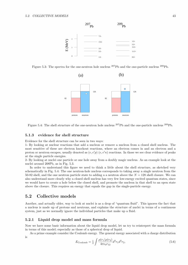
5.2. COLLECTIVE MODELS 43

9/2+

11/2+

15/2-

5/2+

1/2+

1/2-

5/2-

3/2-

7/2-

13/2-

207Pb

0

1

2

E (

MeV

)

Pb209

Figure 5.3: The spectra for the one-neutron hole nucleus 207Pb and the one-particle nucleus 209Pb.

(a) (b)

82

126

protons neutrons

82

126

protons neutrons

Figure 5.4: The shell structure of the one-neutron hole nucleus 207Pb and the one-particle nucleus 209Pb.

5.1.3 evidence for shell structure

Evidence for the shell structure can be seen in two ways:1- By looking at nuclear reactions that add a nucleon or remove a nucleon from a closed shell nucleus. Themost sensitive of these are electron knockout reactions, where an electron comes in and an electron and aproton or neutron escapes, usually denoted as (e, e′p) (e, e′n) reactions. In those we see clear evidence of peaksat the single particle energies.2- By looking at nuclei one particle or one hole away from a doubly magic nucleus. As an example look at thenuclei around 208Pb, as in Fig. 5.3.

In order to understand this figure we need to think a little about the shell structure, as sketched veryschematically in Fig. 5.4: The one neutron-hole nucleus corresponds to taking away a single neutron from the50-82 shell, and the one neutron particle state to adding a a neutron above the N = 128 shell closure. We canalso understand more clearly why a closed shell nucleus has very few low-energy excited quantum states, sincewe would have to create a hole below the closed shell, and promote the nucleon in that shell to an open stateabove the closure. This requires an energy that equals the gap in the single-particle energy.

5.2 Collective models

Another, and actually older, way to look at nuclei is as a drop of “quantum fluid”. This ignores the fact thata nucleus is made up of protons and neutrons, and explains the structure of nuclei in terms of a continuoussystem, just as we normally ignore the individual particles that make up a fluid.

5.2.1 Liquid drop model and mass formula

Now we have some basic information about the liquid drop model, let us try to reinterpret the mass formulain terms of this model; especially as those of a spherical drop of liquid.

As a prime example consider the Coulomb energy. The general energy associated with a charge distributionis

ECoulomb = 12

∫

ρ(r1)ρ(r2)4πε0r12

d3r1d3r2, (5.6)


where the charge distribution is the smeared out charge of the protons,

4π∫ R

0ρ(r)r2dr = Ze (5.7)

If we take the charge to be homogeneously distributed ρ = Ze/(4/3πR3), then

ECoulomb =(2π)(4π)

4πε0ρ2

∫ R

0

∫ 1

−1

r21 dr1 d cos θ r2

2dr2

(r21 + r2

2 − 2r1r2 cos θ)1/2

=πρ2

2ε0

∫ R

0

∫ R

0

(r1 + r2)− |r1 − r2|r1r2

r21dr1 r2

2dr2

=πρ2

2ε0

[

2∫ R

0x2dx

∫ R

0ydy −

∫ R

0

∫ R

0|r1 − r2|r1r2dr1 dr2

]

=πρ2

2ε0

R5

3−R515

=πZ29e2

(4π)2R62ε0

4R5

15=

e2

(4πε0

310

Z2

R. (5.8)

5.2.2 Equilibrium shape & deformation

Once we picture a nucleus as a fluid, we can ask question about its equilibrium shape. From experimentaldata we know that near closed shells nuclei are spherical, i.e., the equilibrium shape is a sphere. When boththe proton and neutron number differ appreciably from the magic numbers, the ground state is often found tobe axially deformed, either prolate (cigar like) or oblate (like a pancake).

A useful analysis to perform is to see what happens when we deform a nucleus slightly, turning it into anellipsoid, with one axis slightly longer than the others, keeping a constant volume:

a = R(1 + ε), b = (R(1 + ε)−1/2. (5.9)

The volume is 43πab2, and is indeed constant. The surface area of an ellipsoid is more complicated, and we

find

S = 2π[

b2 + abarcsin e

e

]

, (5.10)

where the eccentricity e is defined as

e =[

(1− b2/a2]1/2. (5.11)

For small deformation ε we find a much simpler result,

S = 4πR2[

1 +25ε2

]

, (5.12)

and the surface area thus increases for both elongations and contractions. Thus the surface energy increases bythe same factor. There is one competing term, however, since the Coulomb energy also changes, the Coulombenergy goes down, since the particles are further apart,

ECoulomb → ECoulomb

(

1− ε2

5

)

(5.13)

We thus find a change in energy of

DeltaE = ε2[

25βA2/3 − 1

5εZ2A−1/3

]

(5.14)

The spherical shape is stable if ∆E > 0.Since it is found that the nuclear fluid is to very good approximation incompressible, the dynamical

excitations are those where the shape of the nucleus fluctuates, keeping the volume constant, as well asthose where the nucleus rotates without changing its intrinsic shape.

5.2. COLLECTIVE MODELS 45

Figure 5.5: Monopole fluctuations of a liquid drop

Figure 5.6: Dipole fluctuations of a liquid drop

5.2.3 Collective vibrations

Let us first look at collective vibrations, and for simplicity only at those of a spherical fluid drop. Wecan think of a large number of shapes; a complete set can be found by parametrising the surface as r =∑

L,M aLMYLM (θ, φ), where YLM are the spherical harmonics and describe the multipolarity (angular mo-mentum) of the surface. A few examples are shown in Figs. xxx, where we sketch the effects of monopole(L = 0), dipole (L = 1), quadrupole (L = 2) and octupole (L = 3) modes. Let us investigate these modes inturn, in the harmonic limit, where we look at small vibrations (small aLM ) only.

Monopole

The monopole mode, see Fig. 5.5, is the one where the size of the nuclear fluid oscillates, i.e., where the nucleusgets compressed. Experimentally one finds that the lowest excitation of this type, which in even-even nucleicarries the quantum number Jπ = 0+, occurs at an energy of roughly

E0 ≈ 80A−1/3MeV (5.15)

above the ground state. Compared to ordinary nuclear modes, which have energies of a few MeV, these areindeed high energy modes (15 MeV for A = 216), showing the incompressibility of the nuclear fluid.

Dipole

The dipole mode, Fig. 5.6, by itself is not very interesting: it corresponds to an overall translation of the centreof the nuclear fluid. One can, however, imagine a two-fluid model where a proton and neutron fluid oscillateagainst each other. This is a collective isovector (I = 1) mode. It has quantum numbers Jπ = 1−, occurs atan energy of roughly

E0 ≈ 77A−1/3MeV (5.16)

above the ground state, close to the monopole resonance. It shows that the neutron and proton fluids sticktogether quite strongly, and are hard to separate.

Quadrupole

Quadrupole modes, see Fig. 5.7, are the dominant vibrational feature in almost all nuclei. The very specialproperties of the lower multipolarities mean that these are the first modes available for low-energy excitationsin nuclei. In almost all even-even nuclei we find a low-lying state (at excitation energy of less than 1− 2MeV),


Figure 5.7: Quadrupole fluctuations of a liquid drop

Figure 5.8: Octupole fluctuations of a liquid drop

which carries the quantum numbers Jπ = 2+, and near closed shells we can often distinguish the secondharmonic states as well (three states with quantum numbers Jπ = 0+, 2+, 4+) .

Octupole

Octupole modes, with Jπ = 3−, see Fig. 5.8, can be seen in many nuclei. In nuclei where shell-structure makesquadrupole modes occur at very high energies, such as doubly magic nuclei, the octupole state is often thelowest excited state.

5.2.4 Collective rotations

Once we have created a nucleus with axial deformation, i.e., a nucleus with ellipsoidal shape, but still axialsymmetry about one axis, we can rotate the fluid around one of the non-symmetry axes to generate excitations,see Fig. 5.9. We cannot do it around a symmtery axis, since the resulting state would just be the same quantumstate as we started with, and therefore the energy cannot change. A rotated state around a non-symmetryaxis is a different quantum state, and therefore we can overlay many of these states, especially with constantrotational velocity. This is almost like the rotation of a dumbbell, and we can predict the classical spectrumto be of the form

H =12I

J2, (5.17)

Figure 5.9: Collective rotation of an axially deformed liquid drop

5.3. FISSION 47

Figure 5.10: symmetric (upper row) or asymmetric fission (lower row)

R

V(R)

Figure 5.11: potential energy for fission

where J is the classical angular momentum. We predict a quantum mechanical spectrum of the form

Erot(J) =~2

2IJ(J + 1), (5.18)

where J is now the angular momentum quantum number. Naively we expect the spectrum to be morecompressed (the moment of inertial is larger) the more elongated the nucleus becomes. It is known thatcertain structures in nuclei indeed describe well deformed nuclei, up to super and hyper deformed (axis ratiofrom 1 : 1.2 to 1 : 2).

5.3 Fission

Once we have started to look at the liquid drop model, we can try to ask the question what it predicts forfission, where one can use the liquid drop model to good effect. We are studying how a nuclear fluid dropseparates into two smaller ones, either about the same size, or very different in size.

This process is indicated in Fig. 5.10. The liquid drop elongates, by performing either a quadrupole oroctupole type vibration, but it persists until the nucleus falls apart into two pieces. Since the equilibriumshape must be stable against small fluctuations, we find that the energy must go up near the spherical form,as sketched in Fig. 5.11.

In that figure we sketch the energy - which is really the potential energy - for separation into two fragments,R is the fragment distance. As with any of such processes we can either consider classical fission decays forenergy above the fission barrier, or quantum mechanical tunneling for energies below the barrier. The methodused in fission bombs is to use the former, by hitting a 235U nucleus with a slow neutron a state with energyabove the barrier is formed, which fissions fast. The fission products are unstable, and emit additional neutrons,which can give rise to a chain reaction.

The mass formula can be used to give an indication what is going on; Let us look at at the symmetricfusion of a nucleus. In that case the Q value is

Q = M(A,Z)− 2M(A/2, Z/2) (5.19)


R r

V

B V

-U

C C

b

Figure 5.12: The potential energy for alpha decay

Please evaluate this for 236U (92 protons). The mass formula fails in prediciting the asymmetry of fission, thesplitting process is much more likely to go into two unequal fragments.

Missing: Picture of asymmetric fusion.

5.4 Barrier penetration

In order to understand quantum mechanical tunneling in fission it makes sense to look at the simplest fissionprocess: the emission of a He nucleus, so called α radiation. The picture is as in Fig. 5.12.

Suppose there exists an α particle inside a nucleus at an (unbound) energy > 0. Since it isn’t bound, whydoesn’t it decay immediately? This must be tunneling. In the sketch above we have once again shown thenuclear binding potential as a square well, but we have included the Coulomb tail,

VCoulomb(r) =(Z − 2)2e2

4πε0r. (5.20)

. The hight of the barrier is exactly the coulomb potential at the boundary, which is the nuclear readius,RC = 1.2A1.3 fm, and thus BC = 2.4(Z − 2)A−1/3. The decay probablility across a barrier can be given bythe simple integral expression P = e−2γ , with

γ =(2µα)1/2

~

∫ b

RC

[V (r)− Eα]1/2dr

=(2µα)1/2

~

∫ b

RC

[

2(Z − 2)e2

4πε0r− Eα

]1/2

dr

=2(Z − 2)e2

2πε0~v[arccos(Eα/BC)− (Eα/BC)(1− Eα/BC)] , (5.21)

(here v is the velocity associated with Eα). In the limit that BC Eα we find

P = exp[

−2(Z − 2)e2

2ε0~v

]

. (5.22)

This shows how sensitive the probability is to Z and v!

Chapter 6

Some basic concepts of theoreticalparticle physics

We now come to the first hard part of the class. We’ll try to learn what insights we can gain from the equationgoverning relativistic quantum mechanics.

6.1 The difference between relativistic and NR QM

One of the key points in particles physics is that special relativity plays a key role. As you all know, inordinary quantum mechanics we ignore relativity. Of course people attempted to generate equations forrelativistic theories soon after Schrodinger wrote down his equation. There are two such equations, one calledthe Klein-Gordon and the other one called the Dirac equation.

The structure of the ordinary Schrodinger equation of a free particle (no potential) suggests what to do.We can write this equation as

Hψ =1

2mp2ψ = i~ ∂

∂tψ. (6.1)

This is clearly a statement of the non-relativistic energy-momentum relation, E = 12mv2, since a time derivative

on a plane wave brings down a factor energy. Remember, however, that p as an operator also containsderivatives,

p =~i∇. (6.2)

A natural extension would to use the relativistic energy expression,

Hψ =√

m2c4 + p2c2 ψ = i~ ∂∂t

ψ. (6.3)

But this is a nonsensical equation, unless we specify how to take the square root of the operator. The firstattempt to circumvent this problem, by Klein and Gordon, was to take the square of the equation,

(

m2c4 + p2c2) ψ = −~2 ∂2

∂t2ψ. (6.4)

This is an excellent equation for spin-less particles or spin one particles (bosons), but not to describe fermions(half-integer spin), since there is no information about spin is in this equation. This needs careful consideration,since spin must be an intrinsic part of a realtivistic equation!

Dirac realized that there was a way to define the square root of the operator. The trick he used was todefine four matrices α, β that each have the property that their square is one, and that they anticommute,

αiαi = I, ββ = I,

αiβ + βαi = 0, αiαj + αjαi = 0 i 6= j. (6.5)

This then leads to an equation that is linear in the momenta – and very well behaved,

(βmc2 + cα · p)Ψ = i~ ∂∂t

Ψ (6.6)

49

50 CHAPTER 6. SOME BASIC CONCEPTS OF THEORETICAL PARTICLE PHYSICS

Note that the minimum dimension for the matrices in which we can satisfy all conditions is 4, and thus Ψ isa four-vector! This is closely related to the fact that these particles have spin.

Let us investigate this equation a bit further. One of the possible forms of αi and β is

αi =(

0 σi

σi 0

)

, β =(

I 00 −I

)

, (6.7)

where σi are the two-by-two Pauli spin matrices

σ1 =(

0 11 0

)

, σ2 =(

0 −ii 0

)

, σ3 =(

1 00 −1

)

. (6.8)

(These matrices satisfy some very interesting relations. For instance

σ1σ2 = iσ3, σ2σ1 = −iσ3, σ2σ3 = iσ1, (6.9)

etc. Furthermore σ2i = 1.)

Once we know the matrices, we can try to study a plane-wave solution

Ψ(x, t) = u(p)ei(p·x−Et)/~. (6.10)

(Note that the exponent is a “Lorentz scalar”, it is independent of the Lorentz frame!).If substitute this solution we find that u(p) satisfies the eigenvalue equation

mc2 0 p3c p1c− ip2c0 mc2 p1c + ip2c −p3c

p3c p1c− ip2c −mc2 0p1c + ip2c −p3c 0 −mc2

u1u2

u3u4

= E

u1

u2u3

u4

. (6.11)

The eigenvalue problem can be solved easily, and we find the eigenvalue equation

(m2c4 + p2c2 − E2)2 = 0 (6.12)

which has the solutions E = ±√

m2c4 + p2c2. The eigenvectors for the positive eigenvalues are

10

p3c/(E + mc2)(p1c− ip2c)/(E + mc2)

, and

01

(p1c + ip2c)/(E + mc2)−p3c/(E + mc2)

, (6.13)

with similar expressions for the two eigenvectors for the negative energy solutions. In the limit of smallmomentum the positive-energy eigenvectors become

1000

, and

0100

, (6.14)

and seem to denote a particle with spin up and down. We shall show that the other two solutions are relatedto the occurence of anti-particles (positrons).

Just as photons are the best way to analyze (decompose) the electro-magnetic field, electrons and positronsare the natural way way to decompose the Dirac field that is the general solution of the Dirac equation.This analysis of a solution in terms of the particles it contains is called (incorrectly, for historical reasons)“second quantization”, and just means that there is a natural basis in which we can say there is a state atenergy E, which is either full or empty. This could more correctly be referred to as the “occupation numberrepresentation” which should be familiar from condensed matter physics. This helps us to see how a particlecan be described by these wave equations. There is a remaining problem, however!

6.2 Antiparticles

Both the Klein-Gordon and the Dirac equation have a really nasty property. Since the relativistic energyrelation is quadratic, both equations have, for every positive energy solution, a negative energy solution. We

6.3. QED: PHOTON COUPLES TO E+E− 51

mc2

mc2

0

-

E

Figure 6.1: A schematic picture of the levels in the Dirac equation

don’t really wish to see such things, do we? Energies are always positive and this is a real problem. Theresolution is surprisingly simple, but also very profound – It requires us to look at the problem in a verydifferent light.

In figure 6.1 we have sketched the solutions for the Dirac equation for a free particle. It has a positiveenergy spectrum starting at mc2 (you cannot have a particle at lower energy), but also a negative energyspectrum below −mc2. The interpretation of the positive energy states is natural – each state describes aparticle moving at an energy above mc2. Since we cannot have negative energy states, their interpretationmust be very different. The solution is simple: We assume that in an empty vacuum all negative energystates are filled (the “Dirac sea”). Excitations relative to the vacuum can now be obtained by adding particlesat positive energies, or creating holes at negative energies. Creating a hole takes energy, so the hole statesappear at positive energies. They do have opposite charge to the particle states, and thus would correspondto positrons! This shows a great similarity to the behaviour of semiconductors, as you may well know. Thesituation is explained in figure 6.2.

Note that we have ignored the infinite charge of the vacuum (actually, we subtract it away assuminga constant positive background charge.) Removing infinities from calculations is a frequent occurrence inrelativistic quantum theory (RQT). Many unmeasurable quantities become infinite, and we are only interestedin the finite part remaining after removing the infinities. This process is part of what is called renormalisation,which is a systematic procedure to extract finite information from infinite answers!

6.3 QED: photon couples to e+e−

We know that electrons and positrons have charge and thus we need to include electrodynamics in the rela-tivistic quantum theory of the electron. That is even more clear when we take into account that an electronand positron can annihilate by emitting two photons (the well-known 511 keV lines),

e+e− → γγ. (6.15)

Question: Why not one photon?There is a natural way to describe this coupling, in a so-called Lagrangian approach, which I shall not

discuss here. It teaches us that an electron can emit a photon, as indicated figure 6.3.The diagrams in figure 6.3 are usually referred to as a Feynman diagrams, and the process depicted in (a) is

usually called Bremsstrahlung, the one in (b) annihilation. With such a diagram comes a recipe for calculatingit (called the Feynman rule). A key point is that energy and momentum are conserved in all reactions. Let uslook at what happens when another nearby electron absorbs the photon, as in figure 6.4

Of course there are two possibilities: The left electron can emit the photon to the right one, or absorb onethat is emitted by the right one. This is related to the time-ordering of interactions. One of the advantages


mc2

mc2

0

-

E

mc2

mc2

0

-

E

Figure 6.2: A schematic picture of the occupied and empty levels in the Dirac equation. The promotion of aparticle to an empty level corresponds to the creation of a positron-electron pair, and takes an energy largerthan 2mc2.

of feynman diagrams is that both these possibilities are described in one feynman diagram. Thus the time inthis diagram should only be interpreted in the sense of the external lines, what are the particles in and out.It is also very economical if we have more and more particles emitted and aborbed.

Since the emitted photon only lives for a short time, ∆t = ∆x/c, its energy cannot be determined exactlydue to the uncertainty relation

∆E∆t ≥ ~2. (6.16)

Thus even though the sum of the initial (four) momenta, k1 + k2 equals the sum of the final ones, k3 + k4, wefind that the photon does not have to satisfy

q2 = E2q − q2 = 0. (6.17)

Such a photon is called virtual or “off mass-shell”, since it does not satisfy the mass-energy relations. This iswhat gives rise to the Coulomb force.

6.4 Fluctuations of the vacuum

The great problem is in understanding the meaning of virtual particles. Suppose we are studying the vacuumstate in QED. We wish to describe this vacuum in terms of the states of no positrons, electrons and photons(the naive vacuum). Since these particles interact we have short-lived states where e+e− pairs, and photons,and .... appear for a short while and disappear again. This is also true for real particles: a real electron is a“bare” electron surrounded by a cloud of virtual photons, e+e− pairs, etc. A photon can be an e+e− pair partof the time, and more of such anomalies.

6.4.1 Feynman diagrams

As I have sketched above, Feynman diagrams can be used to describe what is happening in these processes.These describe the matrix elements, and the actual transition probability is proportional to the square of thismatrix elements. One can show that each electron-photon coupling vertex is proportional to e, and thus inthe square each vertex gives a factor e2. Actually by drawing time in the vertical direction and space in thehorizontal (schematically, of course), we see that the the two possible couplings of the photon to matter –Bremsstrahlung and pair creation are one and the same process. Still it helps to distinguish. Note that ateach vertex charge is conserved as well as momentum!

6.5. INFINITIES AND RENORMALISATION 53

e-

e-

e-

e-

e-

e-

e

ee

e+

+

+

+

(c) (d)

γ

e+

(e)

γe+

(f)

(a) (b)

γγ

γ γ

t

x

Figure 6.3: The Feynman diagrams for an electron and/or positrons interacting with a photon. Diagram (a)is emission of a photon by an electron, (b) absoption. (c) and (d) are the same diagrams for positrons, and(e) is pair creation, whereas (f) is annihilation.

e-

e- e-

e-

k1

γ

k k

k2

43

q

x

t

Figure 6.4: One of the Feynman diagrams for an electron-electron scattering.

This can actually be combined into a dimensionless quantity

α =e2

4πε0~c≈ 1

137. (6.18)

We should expand in α rather than e2 since expansion parameters, being “unphysical” can not have dimensions.In other words in order to carry through this mathematical concept the natural scale of a diagram is set by thepower of α it carries. Due to the smallness of α we normally consider only the diagrams with as few verticesas possible. Let me list the two diagrams for electron-positron scattering, both proportional to α2, as given infigure 6.6.Question: Why is there only one such diagram for e−e− scattering? Answer: Charge conservation.

We can also construct higher order diagrams, as in figure 6.7.We can also calculate the scattering of light by light, which only comes in at α4, see figure 6.8.The sum of all diagrams contributing to a given process is called the perturbation series.

6.5 Infinities and renormalisation

One of the key features missing in the discussion above is the fact that all the pictures I have drawn are infinite– somewhat of a severe blow. The key point is to understand that this is not a problem, but has to do with a


+=

=

+

+

+

+

+

Figure 6.5: Some Feynman diagrams for “dressed propagators”.

e-

e- e+

e+

e+

e+

e-

e-

γγ

t

x

Figure 6.6: The two Feynman diagrams for an electron-positron scattering.

misinterpretation of the series.When we introduce α and e in our theory these we use the measured value of the charge of an electron

– which is a solution to the full theory, not to the artificial problem with all vacuum fluctuations turned of.What it means is that we should try to express all our answers in physically sensible (measurable) quantities.Renormalisation is the mathematical procedure that does this. A theory (such as QED) is called renormalisableif we can make all expressions finite by reexpressing them in a finite number of physical parameters.

6.6 The predictive power of QED

It is hard to say that a theory has predictive power without comparing it to experiment, so let me highlight afew successes of QED.

One of those is the so-called g factor of the electron, related to the ratio of the spin and orbital contributionsto the magnetic moment. Relativistic theory (i.e., the Dirac equation) shows that g = 2. The measured valuediffers from 2 by a little bit, a fact well accounted for in QED.

experiment g/2 = 1.00115965241(20)Theory g/2 = 1.00115965238(26) (6.19)

Some of the errors in the theory are related to our knowledge of constants such as ~, and require better input.It is also clear that at some scale QCD (the theory of strong interactions) will start playing a role. We areapproaching that limit.

6.7 Problems

1. Discuss the number of different time-orderings of electron-positron scattering in lowest order in α.

6.7. PROBLEMS 55

e-

e- e+

e+

γ

t

x

Figure 6.7: A higher order diagram for electron-positron scattering.

e-

e-

e+e+

γ γ

γγ

Figure 6.8: The lowest diagram for photon-photon scattering.


Chapter 7

The fundamental forces

The fundamental forces are normally divided in four groups, of the four so-called “fundamental” forces. Theseare often naturally classified with respect to a dimensionless measure of their strength. To set these dimensionswe use ~, c and the mass of the proton, mp. The natural classification is then given in table 7.1. Anotherimportant property is their range: the distance to which the interaction can be felt, and the type of quantitythey couple to. Let me look a little closer at each of these in turn.

Table 7.1: A summary of the four fundamental forcesForce Range Strength Acts on

Gravity ∞ GN ≈ 6 10−39 All particles (mass and energy)Weak Force < 10−18m GF ≈ 1 10−5 Leptons, Hadrons

Electromagnetism ∞ α ≈ 1/137 All charged particlesStrong Force ≈ 10−15m g2 ≈ 1 Hadrons

In order to set the scale we need to express everything in a natural set of units. Three scales are providedby ~ and c and e – actually one usually works in units where these two quantities are 1 in high energy physics.For the scale of mass we use the mass of the proton. In summary (for e = 1 we use electron volt as naturalunit of energy)

~ = 6.58× 10−22 MeV s (7.1)

~c = 1.97× 10−13 MeV m (7.2)

mp = 938 MeV/c2 (7.3)

7.1 Gravity

The theory of gravity can be looked at in two ways: The old fashioned Newtonian gravity, where the potentialis proportional to the rest mass of the particles,

V =GNm1m2

r. (7.4)

We find that GNm2p/~c is dimensionless, and takes on the value

GNm2p/~c = 5.9046486× 10−39. (7.5)

There are two more levels to look at gravity. One of those is Einstein’s theory of gravity, which in the low-energy small-mass limit reduces to Newton’s theory. This is still a classical theory, of a classical gravitationalfield.

The quantum theory, where we reexpress the field in their quanta has proven to be a very tough stumblingblock – When one tries to generalise the approach taken for QED, every expression is infinite, and one needsto define an infinite number of different infinite constants. This is not deemed to be acceptable – i.e., it doesn’tdefine a theory. Such a model is called unrenormalisable. We may return to the problem of quantum gravitylater, time permitting.

57

58 CHAPTER 7. THE FUNDAMENTAL FORCES

7.2 Electromagnetism

Electro-magnetism, i.e., QED, has been discussed in some detail in the previous chapter. Look there for adiscussion. The coupling constant for the theory is

α =e2

4πε0~c. (7.6)

7.3 Weak Force

This manifests itself through nuclear β decay,

n → p + e− + νe. (7.7)

The standard coupling for this theory is called the Fermi coupling, GF , after its discoverer. After the theorywas introduced it was learned that there were physical particles that mediate the weak force, the W± and theZ0 bosons. These are very heavy particles (their mass is about 80 times the proton mass!), which is why theyhave such a small range – fluctuations where I need to create that much mass are rare. The W± bosons arecharged, and the Z0 boson is neutral. The typical β decay referred to above is mediated by a W− boson ascan be seen in the Feynman diagram figure 7.1. The reason for this choice is that it conserves charge at eachpoint (the charge of a proton and a W− is zero, the charge of an electron and a neutrino is -1, the same asthat of a W−).

n

p e- νe

W -

Figure 7.1: The Feynman diagram for the weak decay of a neutron.

7.4 Strong Force

The strong force is what keeps nuclei together. It is described by a theory called QCD, which described theforces between fermions called quarks that make up the hadrons. These forces are mediated by spin-1 bosonscalled gluons. Notice that this is a case where a series in powers of the coupling constant does not make a lot ofsense, since higher powers have about the same value as lower powers. Such a theory is called non-perturbative.

Chapter 8

Symmetries and particle physics

Symmetries in physics provide a great fascination to us – one of the hang-ups of mankind. We can recognise asymmetry easily, and they provide a great tool to classify shapes and patterns. There is an important area ofmathematics called group theory, where one studies the transformations under which an object is symmetric.In order to make this statement seem less abstract, let me look at a simple example, a regular hexagon in aplane. As can be seen in figure Fig. 8.5, this object is symmetric (i.e., we can’t distinguish the new from theold object) under rotations around centre over angles of a multiple of 60, and under reflection in any of thesix axes sketched in the second part of the figure.

Figure 8.1: The symmetries of a hexagon

8.1 Importance of symmetries: Noether’s theorem

There are important physical consequences of symmetries in physics, especially if the dynamics of a system isinvariant under a symmetry transformation.

There is a theorem, due to Emily Noether, one of the most important (female) mathematicians of thiscentury, that states that for any continuous symmetry there is a conserved quantity.

So what is a continuous symmetry? Think about something like spherical symmetry – a sphere is invariantunder any rotation about its centre, no matter what the rotation angle. The continuity of choice of parameterin a transformation is what makes the set of transformations continuous. Another way of saying the same thingis that the transformation can be arbitrarily close to the unit transformation, i.e., it can do almost nothing atall.

8.2 Lorenz and Poincare invariance

One of the most common continuous symmetries of a relativistic theory is Lorentz invariance, i.e., the dynamicsis the same in any Lorentz frame. The group of Lorentz transformations can be decomposed into two parts: Pictures!

• Boosts, where we go from one Lorentz frame to another, i.e., we change the velocity.

• Rotations, where we change the orientation of the coordinate frame.

59

60 CHAPTER 8. SYMMETRIES AND PARTICLE PHYSICS

There is a slightly larger group of symmetries, called the Poincare group, obtained when we add translationsto the set of symmetries – clearly the dynamics doesn’t care where we put the orbit of space.

The set of conserved quantities associated with this group is large. Translational and boost invarianceimplies conservation of four momentum, and rotational invariance implies conservation of angular momentum.

8.3 Internal and space-time symmetries

Above I have mentioned angular momentum, the vector product of position and momentum. This is definedin terms of properties of space (or to be more generous, of space-time). But we know that many particlescarry the spin of the particle to form the total angular momentum,

J = L + S. (8.1)

The invariance of the dynamics is such that J is the conserved quantity, which means that we should not justrotate in ordinary space, but in the abstract “intrinsic space” where S is defined. This is something that willoccur several times again, where a symmetry has a combination of a space-time and intrinsic part.

8.4 Discrete Symmetries

Let us first look at the key discrete symmetries – parity P (space inversion) charge conjugation C and time-reversal T .

8.4.1 Parity P

−4 −2 0 2x

−1.0

−0.5

0.0

0.5

1.0

φ

−1.0

−0.5

0.0

0.5

1.0

φ

−4 −2 0 2 4x

n=0

n=2

n=1

n=3

Figure 8.2: The first four harmonic oscillator wave functions

Parity is the transformation where we reflect each point in the origin, x → −x. This transformation shouldbe familiar to you. Let us think of the one dimensional harmonic oscillator, with Hamiltonian

− ~2

2md

dx2 + 12mω2x2. (8.2)

The Hamiltonian does not change under the substitution x → −x. The well-known eigenstates to this problemare either even or odd under this transformation, see Fig. 8.2, and thus have either even or odd parity,

Pψ(x, t) = ψ(−x, t) = ±ψ(x, t), (8.3)

where P is the transformation that take x → −x. For

Pψ(x, t) = ψ(x, t) (8.4)

we say that the state has even parity, for the minus sign we speak about negative parity. These are the onlytwo allowed eigenvalues, as can be seen from looking at the probability density |ψ(x, y)|2. Since this must beinvariant, we find that

|ψ(x, y)|2 = |Pψ(x, y)|2 (8.5)

8.5. THE CPT THEOREM 61

which shows that the only real eigenvalues for P are ±1. One can show that there is a relation between parityand the orbital angular momentum quantum number L, π = (−1)L, which relates two space-time symmetries.

It is found, however, that parity also has an intrinsic part, which is associated with each type of particle.A photon (γ) has negative parity. This can be understood from the following classical analogy. When we lookat Maxwell’s equation for the electric field,

∇ ·E(x, t) =1ε0

ρ(x, t), (8.6)

we find that upon releversal of the coordinates this equation becomes

−∇ ·E(−x, t) =1ε0

ρ(−x, t). (8.7)

The additional minus sign, which originates in the change of sign of ∇ is what gives the electric field and thusthe photon its negative intrinsic parity.

We shall also wish to understand the parity of particles and antiparticles. For fermions (electrons, protons,. . . ) we have the interesting relation PfPf = −1, which will come in handy later!

8.4.2 Charge conjugation C

The name of this symmetry is somewhat of a misnomer. Originally it stems from QED, where it was foundthat a set of interacting electrons behaves exactly the same way as a similar set of positrons. So if we changethe sign of all charges the dynamics is the same. Actually, the symmetry generalises a little bit, and in generalrefers to a transformation where we change all particles in their antiparticles.

Once again we find C2 = 1, and the only possible eigenvalues of this symmetry are ±1. An unchargedparticle like the photon that is its own antiparticle, must be an eigenstate of the symmetry operation, and itis found that it has eigenvalue −1,

Cψγ = −ψγ . (8.8)

(Here ψγ is the wave function of the photon.) This can be shown from Maxwell’s equation (8.6) as before,since ρ chanegs sign under charge conjugation.

For a combination of a particle and an antiparticle, we find that CfCf = −1 for fermions, and +1 forbosons.

8.4.3 Time reversal T

On a microscopic scale it is not very apparent whether time runs forward or backwards, the dynamics wherewe just change the sign of time is equally valid as the original one. This corresponds to flipping the sign of allmomenta in a Feynman diagram, so that incoming particles become outgoing particles and vice-versa. Thissymmetry is slightly nastier, and acts on both space-time and intrinsic quantities such as spin in a complicatedway. The space time part is found to be

Tψ(r, t) = ψ∗(r,−t). (8.9)

Combined with its intrinsic part we find that it has eigenvalues ±i for fermions (electrons, etc.) and ±1 forbosons (photons, etc.).

8.5 The CPT Theorem

A little thought shows that all three symmetries mentioned above appear very natural – but that is a theorist’sargument. The real key test is experiment, not a theorist’s nice ideas! In 1956 C.N. Yang and T.D. Lee analysedthe experimental evidence for these symmetries. They realised there was good evidence of these symmetriesin QED and QCD (the theory of strong interactions). There was no evidence that parity was a symmetry ofthe weak interactions – which was true, since it was shown soon thereafter that these symmetries are broken,in a beautiful experiment led by “Madame” C.S. Wu.

There is a fairly strong proof that only minimal physical assumptions (locality, causality) that the productof C, P and T is a good symmetry of any theory. Up to now experiment has not shown any breaking of thisproduct. We would have to rethink a lot of basic physics if this symmetry is not present. I am reasonablyconfident that if breaking is ever found there will be ten models that can describe it within a month!


8.6 CP violation

The first experimental confirmation of symmetry breaking was found when studying the β− decay of 60Co,

60Co → 60Ni + e− + νe. (8.10)

This nucleus has a ground state with non-zero spin, which can be oriented in a magnetic field.

A magnetic field is a pseudo-vector, which means that under parity it goes over into itself B → B. Sodoes the spin of the nucleus, and we thus have established that under parity the situation under which thenucleus emits electrons should be invariant. But the direction in which they are emitted changes! Thus anyasymmetry between the emission of electrons parallel and anti-parallel to the field implies parity breaking, assketched in figure 8.3.

e-

e-

e-

e-

e-

e-

parity mirror

Figure 8.3: Parity breaking for the β decay of 60Co

Actually one can shown that to high accuracy that the product of C and P is conserved, as can be seen infigure 8.4.

Co60

Co60

Co60

Co60

+e

e+

P C

C P

CP

e

e+

+

e

e

+

+

e-

e-

e-

e-

e-

e-

Figure 8.4: CP symmetry for the β decay of 60Co

8.7. CONTINUOUS SYMMETRIES 63

8.7 Continuous symmetries

8.7.1 Translations

8.7.2 Rotations

8.7.3 Further study of rotational symmetry

Rotational transformations on a wave function can be applied by performing the transformation

exp[i(θxJx + θyJy + θzJz)] (8.11)

on a wave function. This is slightly simpler for a particle without spin, since we shall only have to considerthe orbital angular momentum,

L = p× r = i~r ×∇. (8.12)

Notice that this is still very complicated, exponentials of operators are not easy to deal with. One of the lessonswe learn from applying this operator to many different states, is that if a state has good angular momentum J ,the rotation can transform it into another state of angular momentum J , but it will never change the angularmomentum. This is most easily seen by labelling the states by J,M :

[

J2x + J2

y + J2z

]

φJM = ~2J(J + 1)φJM (8.13)

J2z φJM = MφJM (8.14)

The quantum number M can take the values −J,−J + 1, . . . , J − 1, J , so that we typically have 2J + 1components for each J . The effect of the exponential transformation on a linear combination of states ofidentical J is to perform a linear transformation between these components. I shall show in a minute thatsuch transformation can be implemented by unitary matrices. The transformations that implement thesetransformations are said to correspond to an irreducible representation of the rotation group (often denotedby SO(3)).

Let us look at the simplest example, for spin 1/2. We have two states, one with spin up and one withspin down, ψ±. If the initial state is ψ = α+ψ+ + α−ψ−, the effect of a rotation can only be to turn this intoψ′ = α′+ψ+ + α′−ψ−. Since the transformation is linear (if I rotate the sum of two objects, I might as wellrotate both of them) we find

(

α′+α′−

)

=(

U++ U−+

U+− U−−

)(

α′+α′−

)

(8.15)

Since the transformation can not change the length of the vector, we must have∫

|ψ′|2 = 1. Assuming∫

|ψ±|2 = 1,∫

ψ∗+ψ− = 0 we find

U†U = 1 (8.16)

with

U† =(

U∗++ U∗

+−U∗−+ U∗

−−

)

(8.17)

the so-called hermitian conjugate.We can write down matrices that in the space of S = 1/2 states behave the same as the angular momentum

operators. These are half the well known Pauli matrices

σx =(

0 11 0

)

, σy =(

0 −ii 0

)

, σz =(

1 00 −1

)

. (8.18)

and thus we find thatU(θ) = exp[i(θxσx/2 + θyσy/2 + θzσz/2)]. (8.19)

I don’t really want to discuss how to evaluate the exponent of a matrix, apart from one special case. Supposewe perform a 2π rotation around the z axis, θ = (0, 0, 2π). We find

U(0, 0, 2π) = exp[iπ(

1 00 −1

)

]. (8.20)


Since this matrix is diagonal, we just have to evaluate the exponents for each of the entries (this correspondsto using the Taylor series of the exponential),

U(0, 0, 2π) =(

exp[iπ] 00 exp[−iπ]

)

=(

−1 00 −1

)

. (8.21)

To our surprise this does not take me back to where I started from. Let me make a small demonstration toshow what this means.........

Finally what happens if we combine states from two irreducible representations? Let me analyse this fortwo spin 1/2 states,

ψ = (α1+ψ1

+ + α1−ψ1

−)(α2+ψ2

+ + α2−ψ2

−)

= α1+α2

+ψ1+ψ2

+ + α1+α2

−ψ1+ψ2

− + α1−α2

+ψ1−ψ2

+α1−α2

−ψ1−ψ2

−. (8.22)

The first and the last product of ψ states have an angular momentum component ±1 in the z direction, andmust does at least have J = 1. The middle two combinations with both have M = M1 +M2 = 0 can be shownto be a combination of a J = 1,M = 0 and a J = 0,M = 0 state. Specifically,

1√2

[

ψ1+ψ2

− − ψ1−ψ2

+

]

(8.23)

transforms as a scalar, it goes over into itself. the way to see that is to use the fact that these states transformwith the same U , and substitute these matrices. The result is proportional to where we started from. Noticethat the triplet (S = 1) is symmetric under interchange of the two particles, whereas the singlet (S = 0)is antisymmetric. This relation between symmetry can be exhibited as in the diagrams Fig. ??, where thehorizontal direction denotes symmetry, and the vertical direction denotes antisymmetry. This technique worksfor all unitary groups.....

+x =

Figure 8.5: The Young tableau for the multiplication 1/2× 1/2 = 0 + 1.

The coupling of angular momenta is normally performed through Clebsch-Gordan coefficients, as denotedby

〈j1m1j2m2|JM〉 . (8.24)

We know that M = m1 + m2. Further analysis shows that J can take on all values |j1− j2|, |j1− j2|+ 1, |j1−j2|+ 2, j1 + j2.

8.8 symmetries and selection rules

We shall often use the exact symmetries discussed up till now to determine what is and isn’t allowed. Let us,for instance, look at

8.9 Representations of SU(3) and multiplication rules

A very important group is SU(3), since it is related to the colour carried by the quarks, the basic buildingblocks of QCD.

The transformations within SU(3) are all those amongst a vector consisting of three complex objects thatconserve the length of the vector. These are all three-by-three unitary matrices, which act on the complexvector ψ by

ψ → Uψ

=

U11 U12 U13

U21 U22 U23

U31 U32 U33

ψ1

ψ2

ψ3

(8.25)

8.10. BROKEN SYMMETRIES 65

The complex conjugate vector can be shown to transform as

ψ∗ → ψ∗U†, (8.26)

with the inverse of the matrix. Clearly the fundamental representation of the group, where the matrices repre-senting the transformation are just the matrix transformations, the vectors have length 3. The representationis usually labelled by its number of basis elements as 3. The one the transforms under the inverse matrices isusually denoted by 3.

What happens if we combine two of these objects, ψ and χ∗? It is easy to see that the inner product of ψand χ∗ is scalar,

χ∗ · ψ → χ∗U†Uψ = χ∗ · ψ, (8.27)

where we have used the unitary properties of the matrices the remaining 8 components can all be shown totransform amongst themselves, and we write

3⊗ 3 = 1⊕ 8. (8.28)

Of further interest is the product of three of these vectors,

3⊗ 3⊗ 3 = 1⊕ 8⊕ 8⊕ 10. (8.29)

8.10 broken symmetries

Of course one cannot propose a symmetry, discover that it is not realised in nature (“the symmetry is broken”),and expect that we learn something from that about the physics that is going on. But parity is broken, and westill find it a useful symmetry! That has to do with the manner in which it is broken, only weak interactions– the exchange of W± and Z bosons – break them. Any process mediated by strong, electromagnetic or(probably) gravitational forces conserves the symmetry. This is one example of a symmetry that is only mildlybroken, i.e., where the conserved quantities are still recognisable, even though they are not exactly conserved.

In modern particle physics the way symmetries are broken teaches us a lot about the underlying physics,and it is one of the goals of grand-unified theories (GUTs) to try and understand this.

8.11 Gauge symmetries

One of the things I will not say much about, but which needs to be mentioned, is of a certain class of localsymmetries (i.e., symmetries of the theory at each point in space and time) called gauge symmetries. This is akey idea in almost all modern particle physics theories, so much so that they are usually labelled by the localsymmetry group. Local symmetries are not directly observable, and do not have immediate consequences.They allow for a mathematically consistent and simple formulation of the theories, and in the end predict theparticle that are exchanged – the gauge particles, as summarised in table 8.1.

Table 8.1: The four fundamental forces and their gauge particles

Gravitation graviton(?)QED photonWeak W±, Z0

Strong gluons


Chapter 9

Symmetries of the theory of stronginteractions

The first time people realised the key role of symmetries was in the plethora of particles discovered usingthe first accelerators. Many of those were composite particle (to be explained later) bound by the stronginteraction.

9.1 The first symmetry: isospin

The first particles that show an interesting symmetry are actually the nucleon and the proton. Their massesare remarkably close,

Mp = 939.566 MeV/c2 Mn = 938.272 MeV/c2. (9.1)

If we assume that these masses are generated by the strong interaction there is more than a hint of symmetryhere. Further indications come from the pions: they come in three charge states, and once again their massesare remarkably similar,

Mπ+ = Mπ− = 139.567 MeV/c2, Mπ0 = 134.974 MeV/c2. (9.2)

This symmetry is reinforced by the discovery that the interactions between nucleon (p and n) is independentof charge, they only depend on the nucleon character of these particles – the strong interactions see only onenucleon and one pion. Clearly a continuous transformation between the nucleons and between the pions is asymmetry. The symmetry that was proposed (by Wigner) is an internal symmetry like spin symmetry calledisotopic spin or isospin. It is an abstract rotation in isotopic space, and leads to similar type of states withisotopic spin I = 1/2, 1, 3/2, . . .. One can define the third component of isospin as

Q = e(I3 + B), (9.3)

where B is the baryon number (B = 1 for n, p, 0 for π). We thus find

B Q/e I I3

n 1 0 1/2 −1/2p 1 1 1/2 1/2π− 0 −1 1 −1π0 0 0 1 0π+ 0 1 1 1

(9.4)

Notice that the energy levels of these particles are split by a magnetic force, as ordinary spins split under amagnetic force.

9.2 Strange particles

In 1947 the British physicists Rochester and Butler (from across the street) observed new particles in cosmicray events. (Cosmic rays where the tool before accelerators existed – they are still used due to the unbe-lievably violent processes taking place in the cosmos. We just can’t produce particles like that in the lab.

67

68 CHAPTER 9. SYMMETRIES OF THE THEORY OF STRONG INTERACTIONS

(Un)fortunately the number of highly energetic particles is very low, and we won’t see many events.) Theseparticles came in two forms: a neutral one that decayed into a π+ and a π−, and a positively charge one thatdecayed into a µ+ (heavy electron) and a photon, as sketched in figure 9.1.

π +

π −

V0

V+

+µ

γ

Figure 9.1: The decay of V particles

The big surprise about these particles was how long they lived. There are many decay time scales, buttypically the decay times due to strong interactions are very fast, of the order of a femto second (10−15 s). Thedecay time of the K mesons was about 10−10 s, much more typical of a weak decay. Many similar particleshave since been found, both of mesonic and baryonic type (like pions or like nucleons). These are collectivelyknow as strange particles. Actually, using accelerators it was found that strange particles are typically formedin pairs, e.g.,

π+ + p → Λ0︸︷︷︸

baryon

+ K0︸︷︷︸

meson (9.5)

This mechanism was called associated production, and is highly suggestive of an additive conserved quantity,such as charge, called strangeness. If we assume that the Λ0 has strangeness −1, and the K0 +1, this balances

π+ + p → Λ0 + K0 (9.6)

0 + 0 = −1 + 1 (9.7)

The weak decay

Λ0 → π− + p (9.8)

−1 6= 0 + 0, (9.9)

does not conserve strangeness (but it conserves baryon number). This process is indeed found to take muchlonger, about 10−10 s.

Actually it is found (by analysing many resonance particles) that we can accommodate this quantity inour definition of isospin,

Q = e(I3 +B + S

2) (9.10)

Clearly for S = −1 and B = 1 we get a particle with I3 = 0. This allows us to identify the Λ0 as an I = 0, I3=0

particle, which agrees with the fact that there are no particles of different charge and a similar mass and stronginteraction properties.

The kaons come in three charge states K±, K0 with masses mK± = 494 MeV, mK0 = 498 MeV. Insimilarity with pions, which form an I = 1 multiplet, we would like to assume a I = 1 multiplet of K’s as well.This is problematic since we have to assume S = 1 for all these particles: we cannot satisfy

Q = e(I3 +12) (9.11)

for isospin 1 particles. The other possibility I = 3/2 doesn’t fit with only three particles. Further analysisshows that the the K+ is the antiparticle of K−, but K0 is not its own antiparticle (which is true for the

9.2. STRANGE PARTICLES 69

-1

0

1

-1 0 1

K+

-K

π

0

K

π

K

0

0

S

I3

π- +

Figure 9.2: a possible arrangement for the states of the septet

pions. So we need four particles, and the assignments are S = 1, I = 1/2 for K0 and K−, S = −1, I = 1/2for K+ and K0. Actually, we now realise that we can summarise all the information about K’s and π’s in onemultiplet, suggestive of a (pretty badly broken!) symmetry.

However, it is hard to find a sensible symmetry that gives a 7-dimensional multiplet. It was argued byGell-Mann and Ne’eman in 1961 that a natural extension of isospin symmetry would be an SU(3) symmetry.We have argued before that one of the simplest representations of SU(3) is 8 dimensional symmetry. Amathematical analysis shows that what is missing is a particle with I = I3 = S = 0. Such a particle is known,and is called the η0. The breaking of the symmetry can be seen from the following mass table:

mπ± = 139 MeV

mπ0 = 134 MeV

mK± = 494 MeV

m(−)K0

= 498 MeV

mη0 = 549 MeV

(9.12)

The resulting multiplet is often represented like in figure 9.3.

-1

0

1

-1 0 1

K+

-K

π

0

K

π

K

π η

0

0 0

S

I3

- +

Figure 9.3: Octet of mesons

In order to have the scheme make sense we need to show its predictive power. This was done by studyingthe nucleons and their excited states. Since nucleons have baryon number one, they are labelled with the“hyper-charge” Y ,

Y = (B + S), (9.13)


rather than S. The nucleons form an octet with the single-strangeness particles Λ and σ and the doubly-strangecascade particle Ξ, see figure 9.4.

-1

0

1

-1 0 1

- 0

0 0

I3

Yn p

Σ Λ Σ

Ξ Ξ

Σ- +

Figure 9.4: Octet of nucleons

The masses are

Mn = 938 MeV

Mp = 939 MeV

MΛ0 = 1115 MeV

MΣ+ = 1189 MeV

MΣ0 = 1193 MeV

MΣ− = 1197 MeVMΞ0 = 1315 MeV

MΞ− = 1321 MeV

All these particles were known before the idea of this symmetry. The first confirmation came when studyingthe excited states of the nucleon. Nine states were easily incorporated in a decuplet, and the tenth state (theΩ−, with strangeness -3) was predicted. It was found soon afterwards at the predicted value of the mass.

∆ - ∆ 0 ∆ + ∆ ++

Σ *- Σ *0 Σ *+

Ω-

I3-1 0 1

-2

-1

0

1

Y

ΞΞ *- *0

Figure 9.5: decuplet of excited nucleons

9.3. THE QUARK MODEL OF STRONG INTERACTIONS 71

Table 9.1: The properties of the three quarks.

Quark label spin Q/e I I3 S BUp u 1

2 +23

12 + 1

2 0 13

Down d 12 −1

312 -1

2 0 13

Strange s 12 −1

3 0 0 -1 13

The masses are

M∆ = 1232 MeV

MΣ∗ = 1385 MeV

MΞ∗ = 1530 MeV

MΩ = 1672 MeV

(Notice almost that we can fit these masses as a linear function in Y , as can be seen in figure 9.6. This wasof great help in finding the Ω.)

−2 −1 0 1Y

1.2

1.3

1.4

1.5

1.6

1.7

Mc2 (

GeV

)

Figure 9.6: A linear fit to the mass of the decuplet

9.3 The quark model of strong interactions

Once the eightfold way (as the SU(3) symmetry was poetically referred to) was discovered, the race was on toexplain it. As I have shown before the decaplet and two octets occur in the product

3⊗ 3⊗ 3 = 1⊕ 8⊕ 8⊕ 10. (9.14)

A very natural assumption is to introduce a new particle that comes in three “flavours” called up, down andstrange (u, d and s, respectively), and assume that the baryons are made from three of such particles, and themesons from a quark and anti-quark (remember,

3⊗ 3 = 1⊕ 8. ) (9.15)

Each of these quarks carries one third a unit of baryon number. The properties can now be tabulated, seetable 9.2.

In the multiplet language I used before, we find that the quarks form a triangle, as given in Fig. 9.7.Once we have made this assigment, we can try to derive what combination corresponds to the assignments

of the meson octet, figure 9.8. We just make all possible combinations of a quark and antiquark, apart fromthe scalar one η′ = uu + dd + cc (why?).

A similar assignment can be made for the nucleon octet, and the nucleon decaplet, see e.g., see Fig. 9.9.


-1

0

1

du

-1

0

1

-1 0 1 I3-1 0 1 I3

s

Y d us

Y

Figure 9.7: The multiplet structure of quarks and antiquarks

-1

0

1

-1 0 1

S

I3

ds us

ud uduu-dd

uu+dd-2ss

us ds

Figure 9.8: quark assignment of the meson octet

9.4 SU(4), . . .

Once we have three flavours of quarks, we can ask the question whether more flavours exists. At the momentwe know of three generations of quarks, corresponding to three generations (pairs). These give rise to SU(4),SU(5), SU(6) flavour symmetries. Since the quarks get heavier and heavier, the symmetries get more-and-morebroken as we add flavours.

9.5 Colour symmetry

So why don’t we see fractional charges in nature? This is an important point! In so-called deep inelasticscattering we see pips inside the nucleon – these have been identified as the quarks. We do not see any directsignature of individual quarks. Furthermore, if quarks are fermions, as they are spin 1/2 particles, what aboutantisymmetry of their wavefunction? Let us investigate the ∆++, see Fig. 9.10, which consists of three uquarks with identical spin and flavour (isospin) and symmetric spatial wavefunction,

ψtotal = ψspace × ψspin × ψflavour. (9.16)

This would be symmetric under interchange, which is unacceptable. Actually there is a simple solution. We“just” assume that there is an additional quantity called colour, and take the colour wave function to beantisymmetric:

ψtotal = ψspace × ψspin × ψflavour × ψcolour (9.17)

9.6. THE FEYNMAN DIAGRAMS OF QCD 73

-1

0

1

-1 0 1 I3

Yudd uud

dds uds uds uus

dss uss

Figure 9.9: quark assignment of the nucleon octet

Table 9.2: The properties of the three quarks.

Quark label spin Q/e mass (GEV/c2)Down d 1

2 − 13 0.35

Up u 12 + 2

3 0.35Strange s 1

2 − 13 0.5

Charm c 12 + 2

3 1.5Bottom b 1

2 − 13 4.5

Top t 12 + 2

3 93

We assume that quarks come in three colours. This naturally leads to yet another SU(3) symmetry, which isactually related to the gauge symmetry of strong interactions, QCD. So we have shifted the question to: whycan’t we see coloured particles?

This is a deep and very interesting problem. The only particles that have been seen are colour neutral(“white”) ones. This leads to the assumption of confinement – We cannot liberate coloured particles at “low”energies and temperatures! The question whether they are free at higher energies is an interesting question,and is currently under experimental consideration.

9.6 The feynman diagrams of QCD

There are two key features that distinguish QCD from QED:

1. Quarks interact more strongly the further they are apart, and more weakly as they are close by –assymptotic freedom.

2. Gluons interact with themselves

The first point can only be found through detailed mathematical analysis. It means that free quarks can’t beseen, but at high energies quarks look more and more like free particles. The second statement make QCDso hard to solve. The gluon comes in 8 colour combinations (since it carries a colour and anti-colour index,minus the scalar combination). The relevant diagrams are sketches in Figure 9.11. Try to work out yourselfhow we satisfy colour charge conservation!

9.7 Jets and QCD

One way to see quarks is to use the fact that we can liberate quarks for a short time, at high energy scales.One such process is e+e− → qq, which use the fact that a photon can couple directly to qq. The quarksdon’t live very long and decay by producing a “jet” a shower of particles that results from the deacay of the


( )u u u

( )u u u

Figure 9.10: The ∆++ in the quark model.

q

q

g

g g

g g

g

g

g

Figure 9.11: The basic building blocks for QCD feynman diagrams

quarks. These are all “hadrons”, mesons and baryons, since they must couple through the strong interaction.By determining the energy in each if the two jets we can discover the energy of the initial quarks, and seewhether QCD makes sense.

Chapter 10

Relativistic kinematics

One of the features of particle physics is the importance of special relativity. This occurs at a very fundamentallevel, since particle physics is all about creating and annihilating particles. This can only occur if we canconvert mass to energy and vice-versa. Thus Einstein’s idea of the equivalnece between mass and energyplays an extremely fundamental role in this field of physics. In order for this to be possible we typicallyneed processes that occur at velocities near the light velocity c, so that the kinematics (i.e., the descriptionof momemnta and energy) of these processes requires relativity. In this chapter we shall succintly introducethe few necessary concepts – I hope that for most of you this is a review, but this chapter is intended to beself-contained and contains everything I shall need in relativistic kinematics.

10.1 Lorentz transformations of energy and momentum

As you may know, like we can combine position and time in one four-vector x = (x, ct), we can also combineenergy and momentum in a single four-vector, p = (p, E/c). From the Lorentz transformation property oftime and position, for a change of velocity along the x-axis from a coordinate system at rest to one that ismoving with velocity v = (vx, 0, 0) we have

x′ = γ(v)(x− v/ct), t′ = γ(t− xvx/c2), (10.1)

we can derive that energy and momentum behave in the same way,

p′x = γ(v)(px − Ev/c2) = muxγ(|u|),E′ = γ(v)(E − vpx) = γ(|u|)m0c2. (10.2)

To understand the context of these equations remember the definition of γ

γ(v) = 1/√

1− β2, β =vc. (10.3)

In Eq. (10.2) we have also reexpressed the momentum energy in terms of a velocity u. This is measuredrelative to the rest system of a particle, the system where the three-momentum p = 0.

Now all these exercises would be interesting mathematics but rather futile if there was no further informa-tion. We know however that the full four-momentum is conserved, i.e., if we have two particles coming into acollision and two coming out, the sum of four-momenta before and after is equal,

Ein1 + Ein

2 = Eout1 + Eout

2 ,

pin1 + pin

2 = pout1 + pout

2 . (10.4)

10.2 Invariant mass

One of the key numbers we can extract from mass and momentum is the invariant mass, a number independentof the Lorentz frame we are in

W 2c4 = (∑

i

Ei)2 − (∑

i

pi)2c2. (10.5)

This quantity takes it most transparent form in the centre-of-mass, where∑

i pi = 0. In that case

W = ECM/c2, (10.6)

75

76 CHAPTER 10. RELATIVISTIC KINEMATICS

and is thus, apart from the factor 1/c2, nothing but the energy in the CM frame. For a single particle W = m0,the rest mass.

Most considerations about processes in high energy physics are greatly simplified by concentrating on theinvariant mass. This removes the Lorentz-frame dependence of writing four momenta. I

As an exmaple we look at the collision of a proton and an antiproton at rest, where we produce two quantaof electromagnetic radiation (γ’s), see fig. 10.1, where the anti proton has three-momentum (p, 0, 0), and theproton is at rest.

p p γ

γFigure 10.1: A sketch of a collision between a proton with velocity v and an antiproton at rest producing twogamma quanta.

The four-momenta are

pp = (plab, 0, 0,√

m2pc4 + p2

labc2)

pp = (0, 0, 0,mpc2). (10.7)

From this we find the invariant mass

W =

√

2m2p + 2mp

√

m2p + p2

lab/c2 (10.8)

If the initial momentum is much larger than mp, more accurately

plab mpc, (10.9)

we find thatW ≈

√

2mpplab/c, (10.10)

which energy needs to be shared between the two photons, in equal parts. We could also have chosen to workin the CM frame, where the calculations get a lot easier.

10.3 Transformations between CM and lab frame

Even though the use of the invariant mass simplifies calculations considerably, it clearly does not provide allnecessary information. It does suggest however, that a natural frame to analyse reactions is the CM frame.Often we shall analyse a process in this frame, and use a Lorentz transformation to get informations aboutprocesses in the laboratory frame. Since almost all processes involve the scattering (deflection) of one particleby another (or a number of others), this is natural example for such a procedure, see the sketch in Fig. 10.2.The same procedure can also be applied to the case of production of particles, such as the annihilation processdiscussed above.

Before the collission the beam particle moves with four-momentum

pb = (plab, 0, 0,√

m2bc4 + p2

labc2) (10.11)

and the target particle mt is at rest,pt = (0, 0, 0,mtc2). (10.12)

10.4. ELASTIC-INELASTIC 77

t

tbb

Figure 10.2: A sketch of a collision between two particles

We first need to determine the velocity v of the Lorentz transformation that bring is to the centre-of-massframe. We use the Lorentz transformation rules for momenta to find that in a Lorentz frame moving withvelocity v along the x-axis relative to the CM frame we have

p′bx = γ(v)(plab − vElab/c2)

p′tx = −mtvγ(v). (10.13)

Sine in the CM frame these numbers must be equal in sizebut opposite in sign, we find a linear equation forv, with solution

v =plab

mt + Elab/c2 ≈ c(

1− mt

plab

)

. (10.14)

Now if we know the momentum of the beam particle in the CM frame after collision,

(pf cos θCM, pf sin θCM, 0, E′f ), (10.15)

where θCM is the CM scattering angle we can use the inverse Lorentz transformation, with velocity −v, to tryand find the lab momentum and scattering angle,

γ(v)(pf cos θCM + vE′f/c2) = pf lab cos θlab

pf sin θCM = pf lab sin θlab, (10.16)

from which we concludetan θlab =

1γ(v)

pf sin θCM

pf cos θCM + vE′f/c2 . (10.17)

Of course in experimental situations we shall often wish to transform from lab to CM frames, which can bedone with equal ease.

To understand some of the practical consequences we need to look at the ultra-relativistic limit, whereplab m/c. In that case v ≈ c, and γ(v) ≈ (plab/2mtc2)1/2. This leads to

tan θlab ≈

√

2mtc2

plab

u sin θC

u cos θC + c(10.18)

Here u is the velocity of the particle in the CM frame. This function is always strongly peaked in the forwarddirection unless u ≈ c and cos θC ≈ −1.

10.4 Elastic-inelastic

We shall often be interested in cases where we transfer both energy and momentum from one particle toanother, i.e., we have inelastic collissions where particles change their character – e.g., their rest-mass. If wehave, as in Fig. 10.3, two particles with energy-momentum k1 and pq coming in, and two with k2 and p2

coming out, We know that since energy and momenta are conserved, that k1 + p1 = k2 + p2, which can berearranged to give

p2 = p1 + q, k2 = k1 − q. (10.19)

and shows energy and momentum getting transferred. This picture will occur quite often!

78 CHAPTER 10. RELATIVISTIC KINEMATICS

Figure 10.3: A sketch of a collision between two particles

10.5 Problems

2. Suppose a pion decays into a muon and a neutrino,

π+ = µ+ + νµ. (10.20)

Express the momentum of the muon and the neutrino in terms of the mass of pion and muon. Assume thatthe neutrino mass is zero, and that the pion is at rest. Calculate the momentum using mπ+ = 139.6 MeV/c2,mµ = 105.7 MeV/c2.

3. Calculate the lowest energy at which a Λ(1115) can be produced in a collision of (negative) pionswith protons at rest, throught the reaction π− + p → K0 + Λ. mπ− = 139.6 MeV/c2, mp = 938.3 MeV/c2,mK0 = 497.7 MeV/c2. (Hint: the mass of the Λ is 1115 MeV/c2.)

4. a) Find the maximum value for v such that the relativisitic energy can be expressed by

E ≈ mc2 +p2

2m, (10.21)

with an error of one procent.b) find the minimum value of v and γ so that the relativisitic energy can be expressed by

E ≈ pc, (10.22)

again with an error of one percent.

Documents

Nuclear and Particle Physics