Note on Construction of Expenditure Aggregate and Poverty Lines for IHS2

Introduction The Malawi 2004-2005 Integrated Household Survey (IHS2) was a comprehensive socio-economic survey of the living standards of households in Malawi.1 The National Statistics Office administered the IHS2 household questionnaire to 11,280 households from March 2004-April 2005. The survey was designed so that information gathered could be used for, among other things, an assessment of the incidence of poverty in the population at the district level and above. Poverty is that condition in which basic needs of a household (or individual) are not met. Clearly it is a multidimensional concept. Nevertheless, for purposes of identifying the poor using international standards, a monetary measure is developed as a welfare indicator for each household. Using this monetary measure, households can be ranked from richest to poorest. By developing a poverty line (a monetary threshold, below which a household is labeled as poor), households can be further described as poor or non-poor. For more nuanced classification, multiple poverty lines can be developed, for example, to identify the ultra poor. This note describes the construction of this welfare indicator, referred to as the consumption expenditure aggregate, and the development of poverty lines which can be applied to the welfare indicator to label households as poor. The following sections 2-9 describe how the aggregate was constructed, supplemented by appendices. Consumption Expenditure Aggregate The data on the IHS2 consumption expenditure aggregate is contained in two data sets. The first data set (ihs2_exp.dta) includes real and nominal values of expenditure for each household by disaggregated expenditure categories. The second data (ihs2_pov.dta) collapses the 33 expenditure categories from the first data set into 12 groups and includes the poverty lines and indicators for poor/nonpoor status of the household. ihs2_exp.dta

Following the UN statistical classification system called “Classification of Individual Consumption According to Purpose” (COICOP), consumption related expenditures were coded into 2-digit categories as described in Table A1.1 (see Appendix 1.1 for the 3 digit coding). Expenditures included in each category are only those related to household consumption. Expenditures related to business activities (such as expenditures on fertilizer) were not included. In addition, the list of durable goods for which implied use-value is computed is restricted to

1 An earlier Integrated Household Survey was administered in 1997-98 using a different questionnaire and methodology than the IHS2. For details of the IHS1 and IHS2, see the Basic Information Documents for these surveys published by the National Statistics Office.

those related to consumer durables, and excludes assets or durables related to income-generation (for more information see Section 5).

Broadly speaking, the consumption expenditures fall into four categories:

1) food 2) non-food, non-consumer durables 3) consumer durable goods 4) actual or self-estimated rental cost of housing

In the following sections 3 to 6 there is more information on the calculation of these components of the consumption expenditures. Some general issues to note are:

- Outlier values. Outliers are identified based on a combination of graphical review and standard deviations from means for each subcomponent. Generally, outlier values are replaced by median values based on households in the enumeration area (or by median values at the district/ national level if less than 5 observation at the lower level).

- Annualization. Recall periods for expenditure subcomponents vary, ranging from the last 7 days to the last 12 months. All values are annualized.

- Real values. For each subcomponent, the Malawi Kwacha value is a nominal value. Since the data were collected over 13 months and across different districts, there are price differences which need to be taken into account. In order to compare the monetary values across households, the nominal values are converted to real values to take into account spatial and temporal price differences using a price index developed for this analysis.

ihs2_pov.dta

In order to use consumption expenditure for poverty measurement, the 33 subcomponents in ihs2_exp.dta were summed into 12 categories in ihs2.pov.dta. The relationship between ihs2_pov.dta and ihs2_exp.dta can be seen in Table A1.1. The following exceptions to expenditures in ihs2_pov.dta were made, following recommendations by Deaton and Zaidi (2000):

- Expenditures related to repairs on dwellings were excluded in order to avoid double counting as these items are implicitly included in estimated and actual rental values of the dwelling

- Night’s lodging in rest house or hotel was excluded as a lumpy (rare) expenditure.

In addition to the household real annual expenditures for each of the 12 categories, this data file also includes

- poverty lines (total and ultra-poor poverty lines)

- an indicator variable for whether the household is poor (household per capita consumption below the total poverty line)

- an indicator variable for whether the household is ultra poor (household per capita consumption below the ultra poverty line)

Table 1 - Components of Consumption Expenditures

Component COICOP Code Description

11 Food Food/Beverage

12 Beverage

21 Alcohol Alcohol/Tobacco

22 Tobacco

31 Clothing Clothing/Footwear

32 Footwear

41 Actual rents for housing

42 Estimated rents for housing

43 Regular maintenance and repair of dwelling

Housing/Utilities

45 Electricity, gas, other fuels

51 Decorations, carpets

52 Household textiles

53 Appliances

54 Dishes

55 Tools/equipment for home

Furnishing

56 Routine Home maintenance

61 Health drugs

62 Health out-patient

Health

63 Health hospitalization

71 Vehicles

72 Operation of vehicles

Transport

73 Transport

Communications 81 Communications

91 Audio-visual

92 Major durables for recreation and culture, including repairs

Recreation

94 Recreational and cultural services

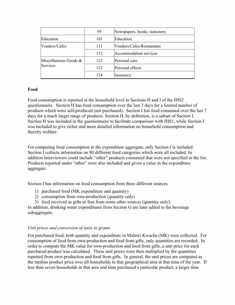
95 Newspapers, books, stationery

Education 101 Education

Vendors/Cafes 111 Vendors/Cafes/Restaurants

112 Accommodation services

121 Personal care

122 Personal effects

Miscellaneous Goods & Services

124 Insurance Food Food consumption is reported at the household level in Sections H and I of the IHS2 questionnaire. Section H has food consumption over the last 3 days for a limited number of products which were self-produced (not purchased). Section I has food consumed over the last 7 days for a much larger range of products. Section H, by definition, is a subset of Section I. Section H was included in the questionnaire to facilitate comparison with IHS1, while Section I was included to give richer and more detailed information on household consumption and thereby welfare.

For computing food consumption in the expenditure aggregate, only Section I is included. Section I collects information on 80 different food categories which were all included. In addition interviewers could include “other” products consumed that were not specified in the list. Products reported under “other” were also included and given a value in the expenditure aggregate.

Section I has information on food consumption from three different sources:

1) purchased food (MK expenditure and quantity) 2) consumption from own-production (quantity only) 3) food received as gifts or free from some other sources (quantity only).

In addition, drinking water expenditures from Section G are later added to the beverage subaggregate.

Unit prices and conversion of units to grams For purchased food, both quantity and expenditure in Malawi Kwacha (MK) were collected. For consumption of food from own-production and food from gifts, only quantities are recorded. In order to compute the MK value for own-production and food from gifts, a unit price for each purchased product was calculated. These unit prices were then multiplied by the quantities reported from own-production and food from gifts. In general, the unit prices are computed as the median product price over all households in that geographical area at that time of the year. If less than seven households in that area and time purchased a particular product, a larger time

span and/or geographical area was used. The use of a minimum seven households to calculate the unit-price guards against high volatility in unit prices over different households.

In the questionnaire, quantities can be reported in 20 different units of measurement. In order to calculate the unit prices and to multiply the quantities with the unit prices, the different units of measurements were all converted into grams. For example, a cup of maize was set equal to 160 grams of maize. Note here that three additional units (spoon, sachet/tube/packet, basin/pot) of measurement were added to the list after the completion of the survey. These units of measurement were all very prominent in the “Other Units” category and it is recommended that these units of measurement are included in future surveys. On the same note was there little reason to have oxcart included in section I, since consumption in a week of any product is extremely unlikely to reach that large a quantity. Finally within each product group (vegetables, cereals etc…) a “other” products is included. Most of these responses have been recoded into already existing product codes, however some answers could not be recoded. The value for these observations was estimated as the median for that product group. Eg. A household reported “22” as an “other vegetable”. This is obviously a mistake, but it is also likely that the household actually consumed something, therefore the value is estimated as the median value for all vegetables.

Non-food, Non-consumer Durables Goods and Services Expenditure on non-food, non-consumer durable goods and services are collected in several sections of the IHS2 household questionnaire. Relevant sections of the questionnaire include sections J, K, L, and G (utilities). The recall period varies across items, depending on the general frequency of purchase. More frequently purchased items have shorter recall periods, while less frequent purchases have long recall periods. The recall periods are last 7 days, last month, last 3 months, and last 12 months. All values are annualized. Education expenditures were reported either by type of expenditure, for example, tuition, books, uniforms, etc., or as an overall total. The total expenditure for education was calculated as the sum of all the sub-categories if they were reported, or as the overall total, whichever is greatest. Consumer Durable Goods Section M of the IHS2 questionnaire collects information on household ownership of 36 durable consumer goods. Seventeen of the items were deemed consumer durables and are included in the consumption expenditure aggregate (see Table 2). They were coded into COICOP subcomponents 53, 55, 71 and 91. The other durable consumer goods are predominately related to income generation or enable higher consumption and, as such, are considered production durables. Therefore, these were excluded. Of course, there are some goods for which it is not clear how to classify them. The assignments used were based on best practices as well as the assignments used in the IHS1 analysis.

As durable consumer goods last for several years, and because it is clearly not the purchase itself of durables that is the relevant component of welfare, they require special treatment when

calculating total expenditure. It is the use of a durable good that contributes to welfare, but since the use is rarely observed directly the yearly use value is estimated (following Deaton & Zaidi, 2002) in the following way:

1) Assuming that each product is uniformly distributed, expected lifetime for each product is calculated as twice the mean age of each product.

2) Remaining lifetime is calculated as current age minus expected lifetime. If current age of product exceeds expected lifetime, remaining lifetime is replaced by two years. The two years were arbitrarily chosen, however other expenditure aggregates have used this value in the past. The yearly use value of each product is then calculated as current value divided by remaining lifetime.

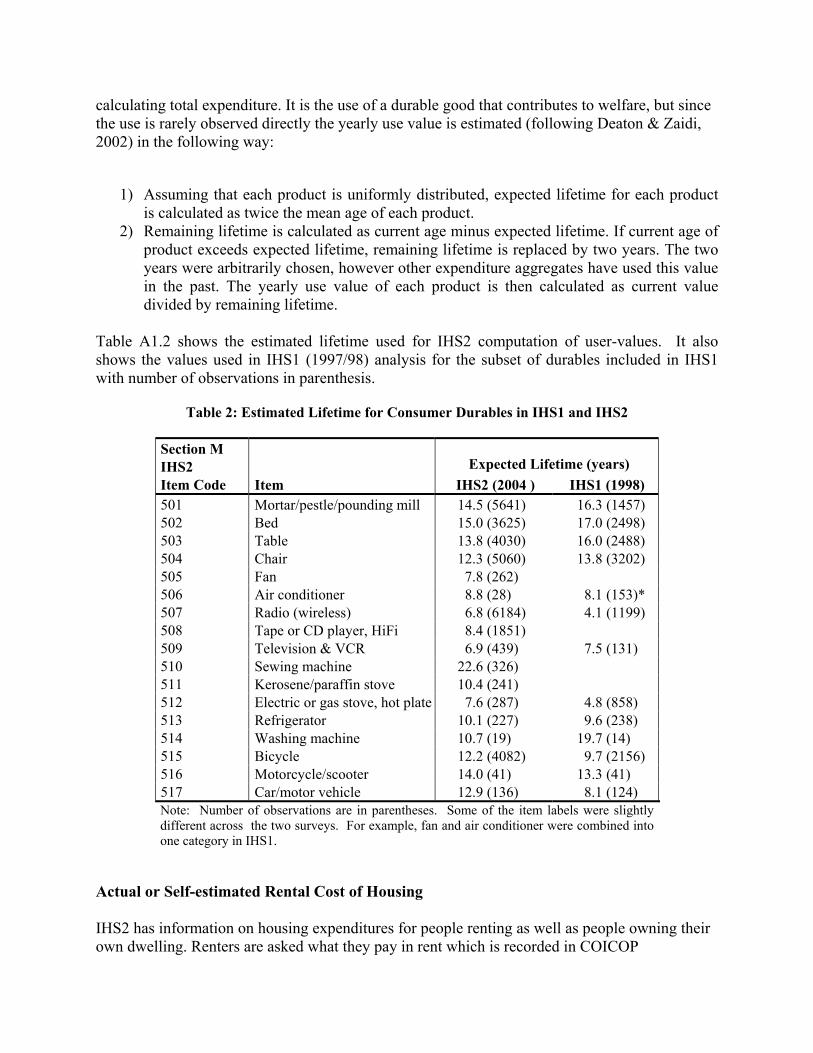
Table A1.2 shows the estimated lifetime used for IHS2 computation of user-values. It also shows the values used in IHS1 (1997/98) analysis for the subset of durables included in IHS1 with number of observations in parenthesis.

Table 2: Estimated Lifetime for Consumer Durables in IHS1 and IHS2

Section M IHS2 Expected Lifetime (years) Item Code Item IHS2 (2004 ) IHS1 (1998) 501 Mortar/pestle/pounding mill 14.5 (5641) 16.3 (1457) 502 Bed 15.0 (3625) 17.0 (2498) 503 Table 13.8 (4030) 16.0 (2488) 504 Chair 12.3 (5060) 13.8 (3202) 505 Fan 7.8 (262) 506 Air conditioner 8.8 (28) 8.1 (153)* 507 Radio (wireless) 6.8 (6184) 4.1 (1199) 508 Tape or CD player, HiFi 8.4 (1851) 509 Television & VCR 6.9 (439) 7.5 (131) 510 Sewing machine 22.6 (326) 511 Kerosene/paraffin stove 10.4 (241) 512 Electric or gas stove, hot plate 7.6 (287) 4.8 (858) 513 Refrigerator 10.1 (227) 9.6 (238) 514 Washing machine 10.7 (19) 19.7 (14) 515 Bicycle 12.2 (4082) 9.7 (2156) 516 Motorcycle/scooter 14.0 (41) 13.3 (41) 517 Car/motor vehicle 12.9 (136) 8.1 (124) Note: Number of observations are in parentheses. Some of the item labels were slightly different across the two surveys. For example, fan and air conditioner were combined into one category in IHS1.

Actual or Self-estimated Rental Cost of Housing IHS2 has information on housing expenditures for people renting as well as people owning their own dwelling. Renters are asked what they pay in rent which is recorded in COICOP

subcomponent 41. People who own their dwelling or do not otherwise pay rent (reside for free) are asked to estimate the rental value of their dwelling if they were to rent it out. The estimated rental value for non-renters is COICOP subcomponent 42. Rental value (actual or self-estimated) is missing for 108 household. For these households, a rental value was imputed based on housing characteristics of similar dwellings in the same areas (urban/rural and actual rent/estimated rent).

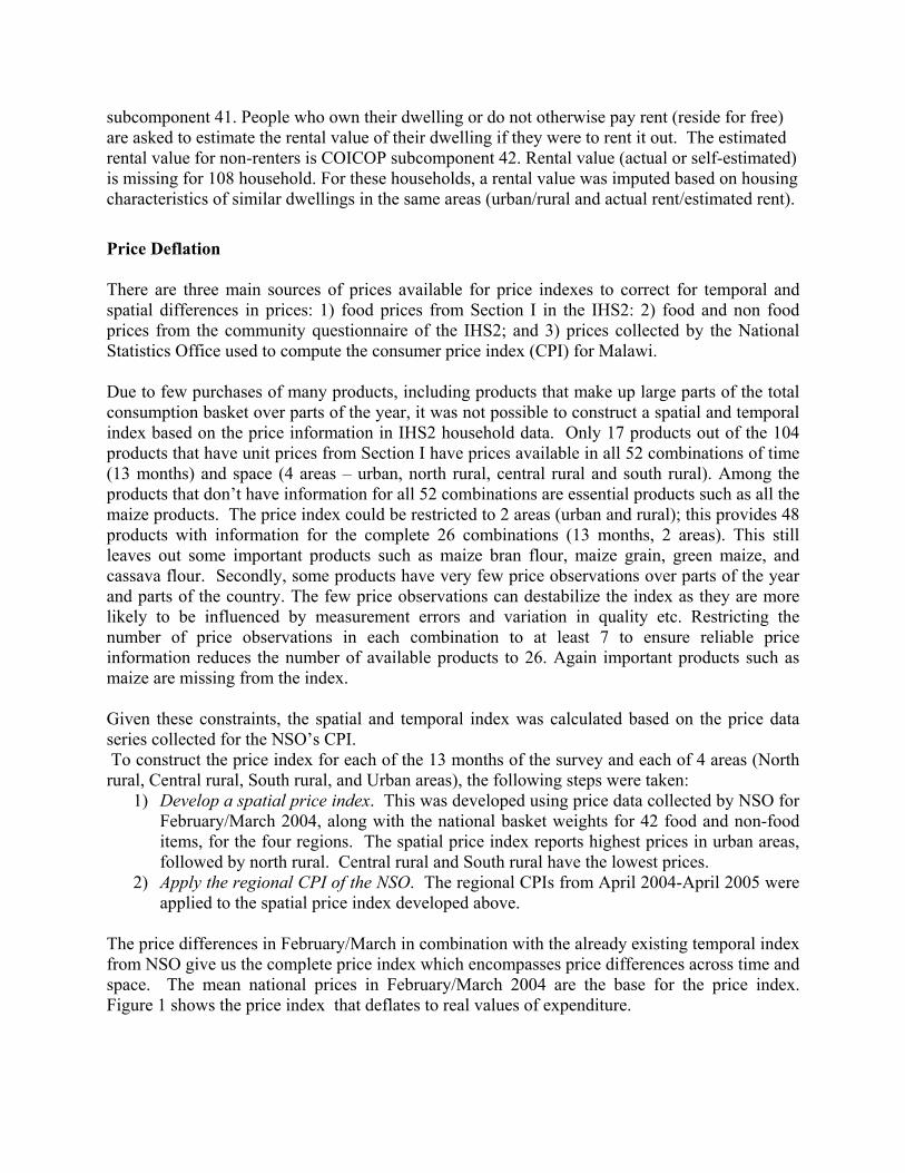
Price Deflation There are three main sources of prices available for price indexes to correct for temporal and spatial differences in prices: 1) food prices from Section I in the IHS2: 2) food and non food prices from the community questionnaire of the IHS2; and 3) prices collected by the National Statistics Office used to compute the consumer price index (CPI) for Malawi. Due to few purchases of many products, including products that make up large parts of the total consumption basket over parts of the year, it was not possible to construct a spatial and temporal index based on the price information in IHS2 household data. Only 17 products out of the 104 products that have unit prices from Section I have prices available in all 52 combinations of time (13 months) and space (4 areas – urban, north rural, central rural and south rural). Among the products that don’t have information for all 52 combinations are essential products such as all the maize products. The price index could be restricted to 2 areas (urban and rural); this provides 48 products with information for the complete 26 combinations (13 months, 2 areas). This still leaves out some important products such as maize bran flour, maize grain, green maize, and cassava flour. Secondly, some products have very few price observations over parts of the year and parts of the country. The few price observations can destabilize the index as they are more likely to be influenced by measurement errors and variation in quality etc. Restricting the number of price observations in each combination to at least 7 to ensure reliable price information reduces the number of available products to 26. Again important products such as maize are missing from the index. Given these constraints, the spatial and temporal index was calculated based on the price data series collected for the NSO’s CPI. To construct the price index for each of the 13 months of the survey and each of 4 areas (North rural, Central rural, South rural, and Urban areas), the following steps were taken:

1) Develop a spatial price index. This was developed using price data collected by NSO for February/March 2004, along with the national basket weights for 42 food and non-food items, for the four regions. The spatial price index reports highest prices in urban areas, followed by north rural. Central rural and South rural have the lowest prices.

2) Apply the regional CPI of the NSO. The regional CPIs from April 2004-April 2005 were applied to the spatial price index developed above.

The price differences in February/March in combination with the already existing temporal index from NSO give us the complete price index which encompasses price differences across time and space. The mean national prices in February/March 2004 are the base for the price index. Figure 1 shows the price index that deflates to real values of expenditure.

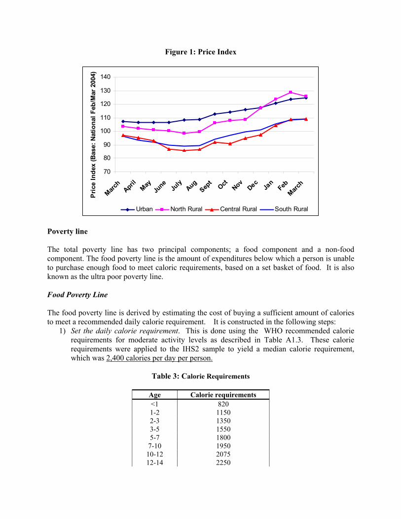
Figure 1: Price Index

70

80

90

100

110

120

130

140

March

April

MayJu

neJu

lyAug

Sept

OctNov

DecJa

nFeb

March

Pric

e In

dex

(Bas

e: N

atio

nal F

eb/M

ar 2

004)

Urban North Rural Central Rural South Rural

Poverty line The total poverty line has two principal components; a food component and a non-food component. The food poverty line is the amount of expenditures below which a person is unable to purchase enough food to meet caloric requirements, based on a set basket of food. It is also known as the ultra poor poverty line. Food Poverty Line The food poverty line is derived by estimating the cost of buying a sufficient amount of calories to meet a recommended daily calorie requirement. It is constructed in the following steps:

1) Set the daily calorie requirement. This is done using the WHO recommended calorie requirements for moderate activity levels as described in Table A1.3. These calorie requirements were applied to the IHS2 sample to yield a median calorie requirement, which was 2,400 calories per day per person.

Table 3: Calorie Requirements

Age Calorie requirements <1 820 1-2 1150 2-3 1350 3-5 1550 5-7 1800

7-10 1950 10-12 2075 12-14 2250

14-16 2400 16-18 2500 18+ 2464

Source: Adapted from the World Health Organization (1985) "Energy and Protein Requirements." WHO Technical Report Series 724. Geneva: World Health Organization.

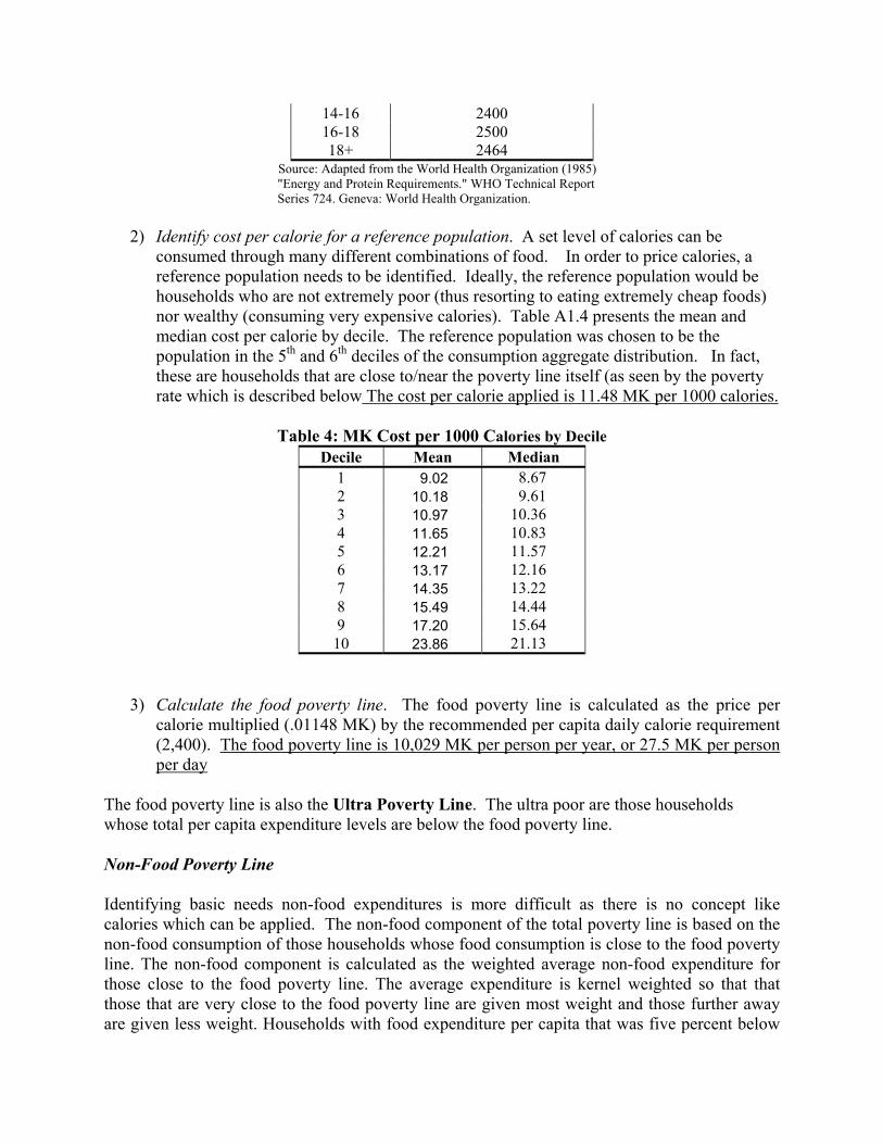
2) Identify cost per calorie for a reference population. A set level of calories can be

consumed through many different combinations of food. In order to price calories, a reference population needs to be identified. Ideally, the reference population would be households who are not extremely poor (thus resorting to eating extremely cheap foods) nor wealthy (consuming very expensive calories). Table A1.4 presents the mean and median cost per calorie by decile. The reference population was chosen to be the population in the 5th and 6th deciles of the consumption aggregate distribution. In fact, these are households that are close to/near the poverty line itself (as seen by the poverty rate which is described below The cost per calorie applied is 11.48 MK per 1000 calories.

Table 4: MK Cost per 1000 Calories by Decile Decile Mean Median

1 9.02 8.67 2 10.18 9.61 3 10.97 10.36 4 11.65 10.83 5 12.21 11.57 6 13.17 12.16 7 14.35 13.22 8 15.49 14.44 9 17.20 15.64

10 23.86 21.13

3) Calculate the food poverty line. The food poverty line is calculated as the price per

calorie multiplied (.01148 MK) by the recommended per capita daily calorie requirement (2,400). The food poverty line is 10,029 MK per person per year, or 27.5 MK per person per day

The food poverty line is also the Ultra Poverty Line. The ultra poor are those households whose total per capita expenditure levels are below the food poverty line. Non-Food Poverty Line Identifying basic needs non-food expenditures is more difficult as there is no concept like calories which can be applied. The non-food component of the total poverty line is based on the non-food consumption of those households whose food consumption is close to the food poverty line. The non-food component is calculated as the weighted average non-food expenditure for those close to the food poverty line. The average expenditure is kernel weighted so that that those that are very close to the food poverty line are given most weight and those further away are given less weight. Households with food expenditure per capita that was five percent below

or above the food poverty line was included in the kernel weighted average. The non-food component of that total poverty line is 6,136 MK per person per year, or 16.8 MK per person per day. . Poverty Line The total poverty line is simply the sum of the food and non-food poverty lines described above. The poverty line is 16,165MK per person per year, or 44.3 MK per person per day. Once the poverty line is established, all households can be categorized as poor or non-poor depending on whether their per capita expenditure (their welfare indicator adjusted for household size) is below or above the poverty line. The poverty headcount, then, can be computed, indicating the proportion of individuals living in poverty. The poverty rate for the population of Malawi is 52.4%. This is the percent of the population whose household per capita consumption is below 16,165MK per year. $1 per day Poverty Estimates

International comparisons of poverty rates are difficult using poverty estimates based on national absolute poverty lines, since different countries set different subsistence minimum standards. Rather, comparisons tend to be made using a fixed poverty line, for example the well-known “$1 per day” poverty estimates. In this approach, the poverty line of $1 per day is converted into local currency units, using the purchasing power parity (PPP) conversion factor rather than exchange rates. To be more precise, the $1 per day poverty line is $32.74 per month (or approximately $1.08 per day). This conversion is defined as the number of units of a country’s currency required to purchase a standard basket of goods and services collected in all countries. The 1993 PPP conversion factor (1.5221) was updated using Malawi CPI inflation rates from 1993 to 2004 (18.48). In 2004, one US dollar is equal to 28.13 Malawi Kwacha using PPP conversion rates. This is equivalent to a “$1 per day” poverty line of 11,051 Kwacha per person per year. The portion of the population living below the “1$ per day” PPP line is 28%. .

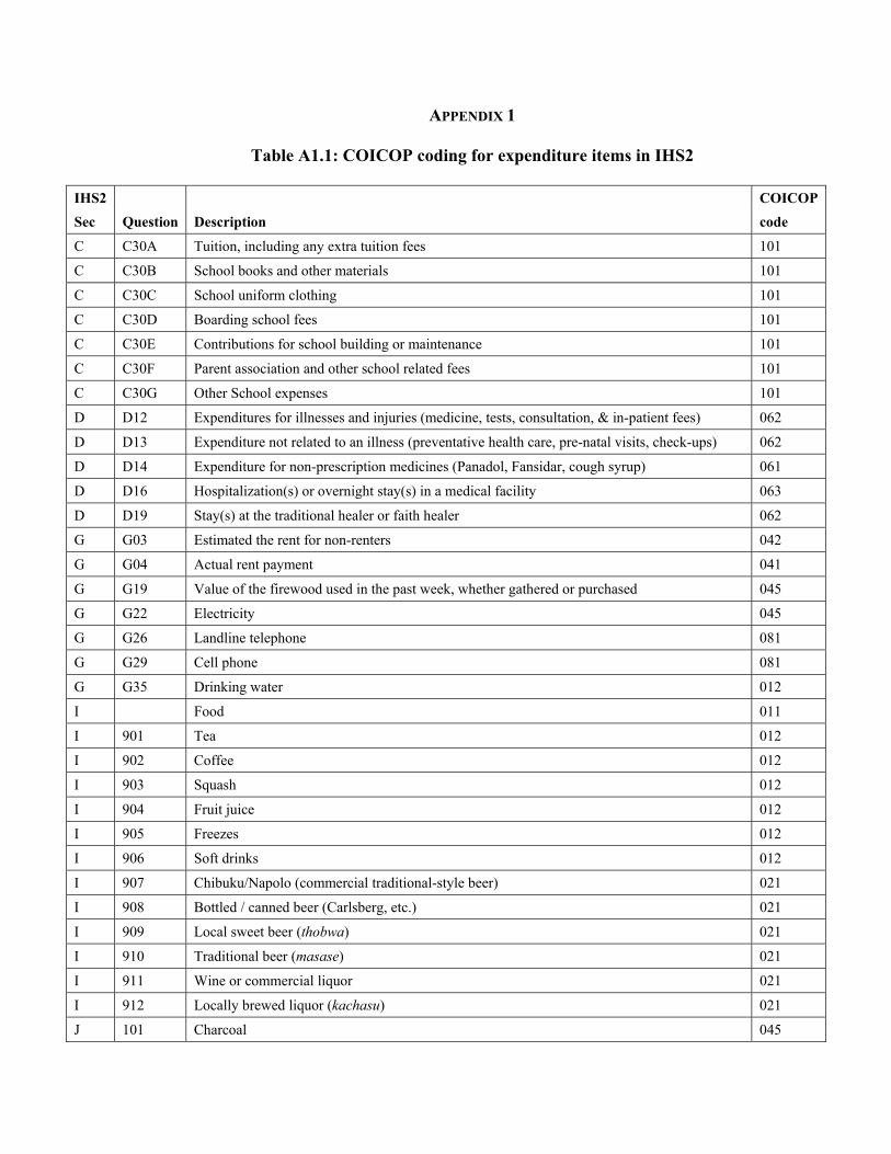
APPENDIX 1

Table A1.1: COICOP coding for expenditure items in IHS2

IHS2 COICOP Sec Question Description code

C C30A Tuition, including any extra tuition fees 101

C C30B School books and other materials 101

C C30C School uniform clothing 101

C C30D Boarding school fees 101

C C30E Contributions for school building or maintenance 101

C C30F Parent association and other school related fees 101

C C30G Other School expenses 101

D D12 Expenditures for illnesses and injuries (medicine, tests, consultation, & in-patient fees) 062

D D13 Expenditure not related to an illness (preventative health care, pre-natal visits, check-ups) 062

D D14 Expenditure for non-prescription medicines (Panadol, Fansidar, cough syrup) 061

D D16 Hospitalization(s) or overnight stay(s) in a medical facility 063

D D19 Stay(s) at the traditional healer or faith healer 062

G G03 Estimated the rent for non-renters 042

G G04 Actual rent payment 041

G G19 Value of the firewood used in the past week, whether gathered or purchased 045

G G22 Electricity 045

G G26 Landline telephone 081

G G29 Cell phone 081

G G35 Drinking water 012

I Food 011

I 901 Tea 012

I 902 Coffee 012

I 903 Squash 012

I 904 Fruit juice 012

I 905 Freezes 012

I 906 Soft drinks 012

I 907 Chibuku/Napolo (commercial traditional-style beer) 021

I 908 Bottled / canned beer (Carlsberg, etc.) 021

I 909 Local sweet beer (thobwa) 021

I 910 Traditional beer (masase) 021

I 911 Wine or commercial liquor 021

I 912 Locally brewed liquor (kachasu) 021

J 101 Charcoal 045

IHS2 COICOP Sec Question Description code

J 102 Paraffin or kerosene 045

J 103 Cigarettes or other tobacco 022

J 104 Matches 045

J 105 Newspapers or magazines 095

J 106 Public transport – bus fare, taxi fare 073

J 201 Milling fees, grain 056

J 202 Bar soap (body soap or clothes soap) 122

J 203 Clothes soap (powder) 122

J 204 Toothpaste, toothbrush 122

J 205 Toilet paper 122

J 206 Glycerine, Vaseline, skin creams 122

J 207 Other personal products (shampoo, razor blades, cosmetics, hair products, etc.) 122

J 208 Household cleaning products (dish soap, toilet cleansers, etc.) 056

J 209 Light bulbs 045

J 210 Postage stamps or other postal fees 081

J 212 Petrol or diesel 072

J 213 Motor vehicle service, repair, or parts 072

J 214 Bicycle service, repair, or parts 072

J 215 Wages paid to servants 056

J 218 Repairs to household and personal items (radios, watches, etc.) 053

K 301 Infant clothing 031

K 302 Baby nappies/diapers 031

K 303 Boy's trousers 031

K 304 Boy's shirts 031

K 305 Boy's jackets 031

K 306 Boy's undergarments 031

K 307 Boy's other clothing 031

K 308 Men's trousers 031

K 309 Men's shirts 031

K 310 Men's jackets 031

K 311 Men's undergarments 031

K 312 Men's other clothing 031

K 313 Girl's blouse/shirt 031

K 314 Girl's dress/skirt 031

K 315 Girl's undergarments 031

K 316 Girl's other clothing 031

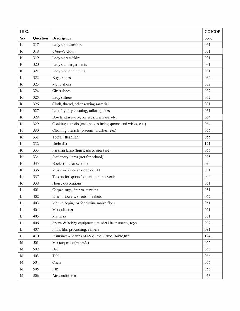
IHS2 COICOP Sec Question Description code

K 317 Lady's blouse/shirt 031

K 318 Chitenje cloth 031

K 319 Lady's dress/skirt 031

K 320 Lady's undergarments 031

K 321 Lady's other clothing 031

K 322 Boy's shoes 032

K 323 Men's shoes 032

K 324 Girl's shoes 032

K 325 Lady's shoes 032

K 326 Cloth, thread, other sewing material 031

K 327 Laundry, dry cleaning, tailoring fees 031

K 328 Bowls, glassware, plates, silverware, etc. 054

K 329 Cooking utensils (cookpots, stirring spoons and wisks, etc.) 054

K 330 Cleaning utensils (brooms, brushes, etc.) 056

K 331 Torch / flashlight 055

K 332 Umbrella 121

K 333 Paraffin lamp (hurricane or pressure) 055

K 334 Stationery items (not for school) 095

K 335 Books (not for school) 095

K 336 Music or video cassette or CD 091

K 337 Tickets for sports / entertainment events 094

K 338 House decorations 051

L 401 Carpet, rugs, drapes, curtains 051

L 402 Linen - towels, sheets, blankets 052

L 403 Mat - sleeping or for drying maize flour 051

L 404 Mosquito net 051

L 405 Mattress 051

L 406 Sports & hobby equipment, musical instruments, toys 092

L 407 Film, film processing, camera 091

L 410 Insurance - health (MASM, etc.), auto, home,life 124

M 501 Mortar/pestle (mtondo) 055

M 502 Bed 056

M 503 Table 056

M 504 Chair 056

M 505 Fan 056

M 506 Air conditioner 053

IHS2 COICOP Sec Question Description code

M 507 Radio (wireless) 091

M 508 Tape or CD player; HiFi 091

M 509 Television & VCR 091

M 510 Sewing machine 053

M 511 Kerosene/paraffin stove 053

M 512 Electric or gas stove; hot plate 053

M 513 Refrigerator 053

M 514 Washing machine 053

M 515 Bicycle 071

M 516 Motorcycle/scooter 071

M 517 Car 071

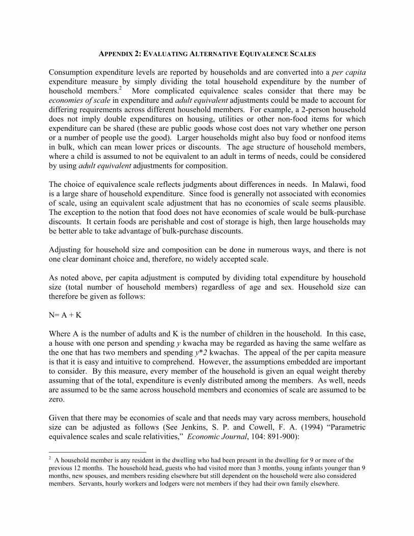
APPENDIX 2: EVALUATING ALTERNATIVE EQUIVALENCE SCALES Consumption expenditure levels are reported by households and are converted into a per capita expenditure measure by simply dividing the total household expenditure by the number of household members.2 More complicated equivalence scales consider that there may be economies of scale in expenditure and adult equivalent adjustments could be made to account for differing requirements across different household members. For example, a 2-person household does not imply double expenditures on housing, utilities or other non-food items for which expenditure can be shared (these are public goods whose cost does not vary whether one person or a number of people use the good). Larger households might also buy food or nonfood items in bulk, which can mean lower prices or discounts. The age structure of household members, where a child is assumed to not be equivalent to an adult in terms of needs, could be considered by using adult equivalent adjustments for composition. The choice of equivalence scale reflects judgments about differences in needs. In Malawi, food is a large share of household expenditure. Since food is generally not associated with economies of scale, using an equivalent scale adjustment that has no economies of scale seems plausible. The exception to the notion that food does not have economies of scale would be bulk-purchase discounts. It certain foods are perishable and cost of storage is high, then large households may be better able to take advantage of bulk-purchase discounts. Adjusting for household size and composition can be done in numerous ways, and there is not one clear dominant choice and, therefore, no widely accepted scale. As noted above, per capita adjustment is computed by dividing total expenditure by household size (total number of household members) regardless of age and sex. Household size can therefore be given as follows: N= A + K Where A is the number of adults and K is the number of children in the household. In this case, a house with one person and spending y kwacha may be regarded as having the same welfare as the one that has two members and spending y*2 kwachas. The appeal of the per capita measure is that it is easy and intuitive to comprehend. However, the assumptions embedded are important to consider. By this measure, every member of the household is given an equal weight thereby assuming that of the total, expenditure is evenly distributed among the members. As well, needs are assumed to be the same across household members and economies of scale are assumed to be zero. Given that there may be economies of scale and that needs may vary across members, household size can be adjusted as follows (See Jenkins, S. P. and Cowell, F. A. (1994) “Parametric equivalence scales and scale relativities,” Economic Journal, 104: 891-900):

2 A household member is any resident in the dwelling who had been present in the dwelling for 9 or more of the previous 12 months. The household head, guests who had visited more than 3 months, young infants younger than 9 months, new spouses, and members residing elsewhere but still dependent on the household were also considered members. Servants, hourly workers and lodgers were not members if they had their own family elsewhere.

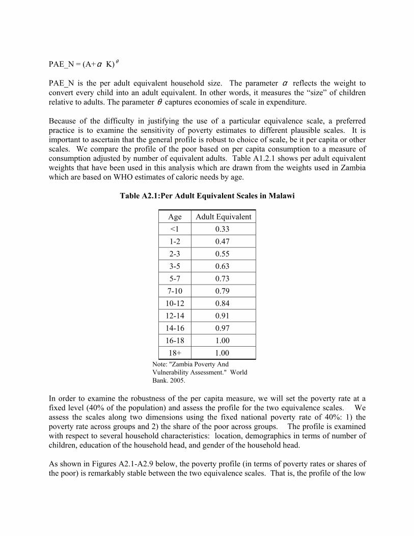
PAE_N = (A+α K) θ PAE_N is the per adult equivalent household size. The parameter α reflects the weight to convert every child into an adult equivalent. In other words, it measures the “size” of children relative to adults. The parameter θ captures economies of scale in expenditure. Because of the difficulty in justifying the use of a particular equivalence scale, a preferred practice is to examine the sensitivity of poverty estimates to different plausible scales. It is important to ascertain that the general profile is robust to choice of scale, be it per capita or other scales. We compare the profile of the poor based on per capita consumption to a measure of consumption adjusted by number of equivalent adults. Table A1.2.1 shows per adult equivalent weights that have been used in this analysis which are drawn from the weights used in Zambia which are based on WHO estimates of caloric needs by age.

Table A2.1:Per Adult Equivalent Scales in Malawi

Age Adult Equivalent <1 0.33 1-2 0.47 2-3 0.55 3-5 0.63 5-7 0.73 7-10 0.79 10-12 0.84 12-14 0.91 14-16 0.97 16-18 1.00 18+ 1.00

Note: "Zambia Poverty And Vulnerability Assessment." World Bank. 2005.

In order to examine the robustness of the per capita measure, we will set the poverty rate at a fixed level (40% of the population) and assess the profile for the two equivalence scales. We assess the scales along two dimensions using the fixed national poverty rate of 40%: 1) the poverty rate across groups and 2) the share of the poor across groups. The profile is examined with respect to several household characteristics: location, demographics in terms of number of children, education of the household head, and gender of the household head. As shown in Figures A2.1-A2.9 below, the poverty profile (in terms of poverty rates or shares of the poor) is remarkably stable between the two equivalence scales. That is, the profile of the low

income population is similar regardless of the use of per capita scales or scales based on equivalence weights in Table A1.2.1.

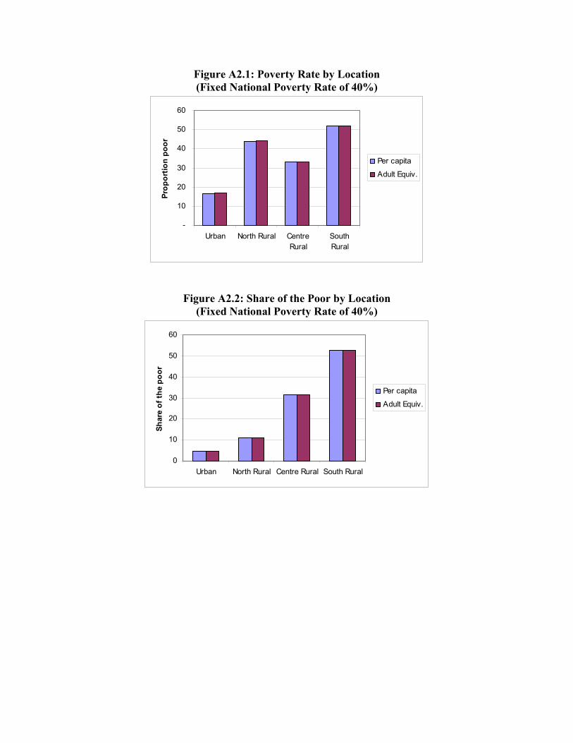
Figure A2.1: Poverty Rate by Location (Fixed National Poverty Rate of 40%)

-

10

20

30

40

50

60

Urban North Rural CentreRural

SouthRural

Prop

ortio

n po

or

Per capita

Adult Equiv.

Figure A2.2: Share of the Poor by Location (Fixed National Poverty Rate of 40%)

0

10

20

30

40

50

60

Urban North Rural Centre Rural South Rural

Shar

e of

the

poor

Per capita

Adult Equiv.

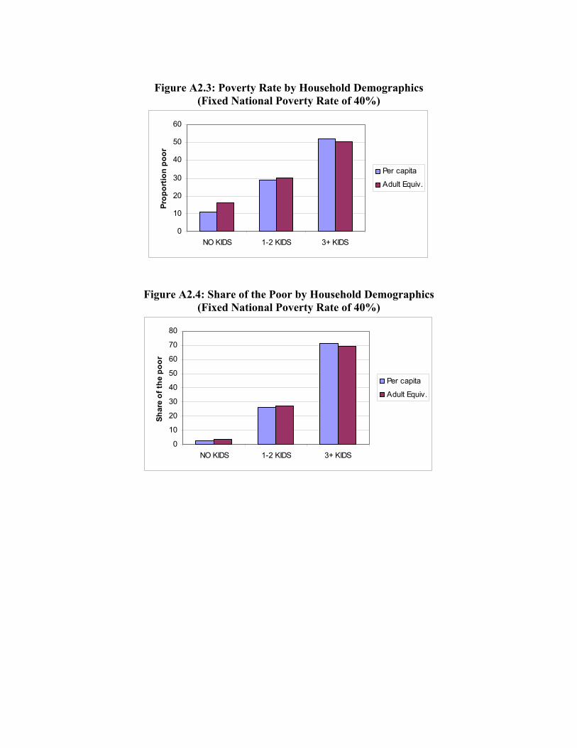
Figure A2.3: Poverty Rate by Household Demographics

(Fixed National Poverty Rate of 40%)

0

10

20

30

40

50

60

NO KIDS 1-2 KIDS 3+ KIDS

Prop

ortio

n po

or

Per capita

Adult Equiv.

Figure A2.4: Share of the Poor by Household Demographics (Fixed National Poverty Rate of 40%)

0

10

20

30

40

50

60

70

80

NO KIDS 1-2 KIDS 3+ KIDS

Shar

e of

the

poor

Per capita

Adult Equiv.

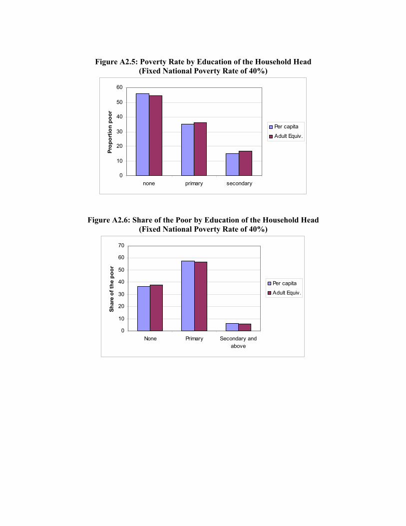
Figure A2.5: Poverty Rate by Education of the Household Head

(Fixed National Poverty Rate of 40%)

0

10

20

30

40

50

60

none primary secondary

Prop

ortio

n po

or

Per capita

Adult Equiv.

Figure A2.6: Share of the Poor by Education of the Household Head (Fixed National Poverty Rate of 40%)

0

10

20

30

40

50

60

70

None Primary Secondary andabove

Shar

e of

the

poor

Per capita

Adult Equiv.

Figure A2.7: Poverty Rate by Gender of the Household Head

(Fixed National Poverty Rate of 40%)

0

10

20

30

40

50

60

Male Female

Prop

ortio

n po

or

Per capitaAdult Equiv.

Figure A2.8: Poverty Rate by Gender of the Household Head and Location (Fixed National Poverty Rate of 40%)

0

10

20

30

40

50

60

Percapita

AdultEquiv.

Percapita

AdultEquiv.

male female

UrbanNorth RuralCentre RuralSouth Rural

Figure A2.9: Share of the Poor by Gender of the Household Head

(Fixed National Poverty Rate of 40%)

010

203040

506070

8090

male female

Shar

e of

thep

oor

Per capita

Adult Equiv.

Appendix 3 Imputations for Dowa district The consumption expenditure aggregate for the Dowa district has been replaced by imputed values. To impute values for the Dowa district the following three steps were followed. First, we developed a regression model that explains the relationship between real per capita expenditure consumption and non-expenditure variables as household composition, employment etc. The model used to impute values was based on regressions of per capita expenditure from the neighboring districts of Ntchisi, Lilongwe Rural and Kasungu. Secondly, we impute total expenditure aggregate in Dowa based on the relationship between total per capita expenditure consumption and non-expenditure variables established from the neighboring districts. The methodology applied builds on recent methodological developments in survey-to-survey imputations. It is superior to regular regression analysis as it builds on the entire distribution and not only the mean. 100 simulations of per capita expenditure were done for the Dowa district. The median value of the simulations was used for the final value. (See Elbers, Chris, Jean O. Lanjouw, and Peter Lanjouw. 2004. “Imputed Welfare Estimates in Regression Analysis”. Policy Research Working Paper 3294. The World Bank, Development Research Group, Poverty Team, May.) We used the povmap program which applies the methodology noted above. (The povmap program is a program developed by the World Bank which is designed to make poverty maps based on a survey and a census, as well as survey-to-survey imputations. The program is still under development.) For the simulations, 100 simulations were run, using non-parametric distributions for both cluster draws and household draws. The following broad categories of variables were included in the model: household composition (size, number of dependents etc), education, assets (ownership of chair etc), employment (percentage on labor market, household has enterprise, engaged in agriculture etc.), and community characteristics (eg. trading market). Finally, imputed values of the consumption expenditure subcomponents were based on the imputed total expenditure aggregate and the proportion of each subcomponent in the actual (non-imputed) data. For example if a household spent 60 percent of their non-imputed total consumption expenditure on food, they also spent 60 percent of their imputed total consumption expenditure on food.