Normal and shear strain imaging using 2D deformation tracking on beamsteered linear array datasets

Haiyan Xua) and Tomy Vargheseb)

Department of Medical Physics, University of Wisconsin–Madison, Madison, Wisconsin 53705 and Departmentof Electrical and Computer Engineering, University of Wisconsin–Madison, Madison, Wisconsin 53705

(Received 6 July 2012; revised 14 November 2012; accepted for publication 15 November 2012;published 20 December 2012)

Purpose: Previous publications have reported on the use of one-dimensional cross-correlation anal-ysis with beam-steered echo signals. However, this approach fails to accurately track displacementsat larger depths (>4.5 cm) due to lower signal-to-noise. In this paper, the authors present the use ofadaptive parallelogram shaped two-dimensional processing blocks for deformation tracking.Methods: Beam-steered datasets were acquired using a VFX 9L4 linear array transducer operated ata 6 MHz center frequency for steered angles from −15 to 15◦ in increments of 1◦, on both uniformlyelastic and single-inclusion tissue-mimicking phantoms. Echo signals were acquired to a depth of65 mm with the focus set at 40 mm corresponding to the center of phantom. Estimated angulardisplacements along and perpendicular to the beam direction are used to compute axial and lateraldisplacement vectors using a least-squares approach. Normal and shear strain tensor component arethen estimated based on these displacement vectors.Results: Their results demonstrate that parallelogram shaped two-dimensional deformation trackingsignificantly improves spatial resolution (factor of 7.79 along the beam direction), signal-to-noise(5 dB improvement), and contrast-to-noise (8–14 dB improvement) associated with strain imagingusing beam steering on linear array transducers.Conclusions: Parallelogram shaped two-dimensional deformation tracking is demonstrated in beam-steered radiofrequency data, enabling its use in the estimation of normal and shear strain components.© 2013 American Association of Physicists in Medicine. [http://dx.doi.org/10.1118/1.4770272]

Key words: breast cancer, beam steering, angular compounding, normal and shear strain

I. INTRODUCTION

Feasibility of utilizing shear strain imaging to classify anddifferentiate benign from malignant breast masses based ontheir bonding information (lesion mobility) has been shownin previous in vivo studies.1–4 However, due to the signifi-cantly lower lateral resolution associated with current clinicalultrasound systems, when compared to the axial resolution,most of the studies utilize only the axial-shear strain compo-nent instead of the full-shear strain component.2, 3 Our previ-ous comparison study between the axial-shear and full-shearstrain tensor demonstrate that full-shear strain imaging pro-vides improved accuracy and robust results for breast tumorclassification, especially for asymmetrical positioning of themass with respect to the applied deformation.1 Accurate es-timation of the lateral displacement vector and strain tensorcan help improve the feasibility of utilizing full-shear strainimaging and thereby improve breast tumor classification.

Spatial resolution describes a system’s ability to distin-guish between two closely situated objects, and includes boththe axial resolution (along beam direction) and lateral resolu-tion (perpendicular to beam direction). Previous studies havedemonstrated tradeoffs between the elastographic signal-to-noise ratio (SNRe), contrast-to-noise ratio (CNRe), and ax-ial resolution.5–7 In general, larger cross-correlation windowlengths for 1D processing5–7 and kernel dimensions for two-dimensional (2D) processing may improve SNRe and CNRe

at the cost of the axial resolution.7 The effort on improving

spatial resolution has focused on reduction in the windowlengths for 1D processing5–8 and kernel dimensions for 2Dprocessing.2, 9 On the other hand, lateral resolution for 1Dprocessing is primarily affected by the beam width and linedensity.10 However, there was no statistically significant re-lationship associated with lateral resolution and 1D windowlength.10 Further study is required to determine the impact ofthe lateral extent of the 2D kernel on lateral spatial resolutionwith 2D processing.

Different approaches have been developed to improvelateral displacement estimation as described in previouslypublished studies.11–25 Methods proposed include use ofthe tissue incompressibility assumption,16 interpolation be-tween radiofrequency (RF) lines19, 20 to improve the linedensity, interpolation for cross-correlation displacementtracking17, 18, 25 to provide subsample estimation of the dis-placement, multidimensional processing,23, 24 and angularinsonifications.11–15, 21, 26–30

Our group has developed novel approaches that utilize an-gular displacements estimated from beam-steered RF echodata pairs to improve accuracy of the estimated lateraldisplacement vector.13, 15, 26 Based on the assumption thatnoise artifacts are independent and identically distributed,Techavipoo et al.27, 28 developed a least-squares approachto estimate both normal and shear strain tensors using RFdata acquired with phased array transducers. Rao et al.12, 29

modified this approach for linear array transducers using 1Dcross-correlation based analysis. In addition, Rao et al.14 also

012902-1 Med. Phys. 40 (1), January 2013 © 2013 Am. Assoc. Phys. Med. 012902-10094-2405/2013/40(1)/012902/13/$30.00

012902-2 H. Xu and T. Varghese: 2D deformation tracking on beam steered linear array datasets 012902-2

implemented an approach using lateral shear deformations.Quantitative experimental results with spatial angular com-pounding demonstrate that least-squares compounding pro-vides significant improvement in the SNRe and CNRe, whencompared to weighted-compounding.11 Chen and Varghese26

extended the least-squares approach by incorporating a cross-correlation matrix of displacement noise errors into the strainestimation process thereby avoiding any other assumptionsfor simplifying estimation noise. In addition, angular com-pounding has been used to estimate variations in attenuationto reduce shadowing of spatially compounded images31 andfor Young’s modulus32 reconstructions.

We have previously demonstrated the presence of decor-relation noise artifacts associated with 1D cross correlationbased deformation tracking especially at increased depthsin a phantom.1 This is due to the reduced sonographicSNR associated with echo signals at deeper locations dueto tissue attenuation.33 A more robust deformation trackingapproach is therefore necessary. Hansen et al.21 presenteda approach utilizing 2D block matching based deformationtracking to estimate axial displacements. However, this ap-proach utilizes lateral displacement information from onlytwo beam-steered angles and utilize a geometrical rotationaltransformation to register these displacements onto the 0◦

Cartesian spatial grid.15, 27 Azar et al.30 have also demon-strated the improved performance of 2D tracking using beamsteering for estimating the lateral component of the displace-ment vector.

In this paper, we present the use of parallelogram shaped2D processing blocks for deformation tracking that vary withthe beam-steering angle to estimate the 2D angular displace-ment vector under a quasistatic deformation.34 Orthogonal ax-ial and lateral components are then estimated from the 2Dangular displacements after a geometrical shear transforma-tion to first register these displacements onto the 0◦ Cartesianspatial grid and utilizing a least-squares approach. A gradi-

ent of the axial displacement vector is utilized to estimateaxial strain and axial-shear strain tensors. In a similar man-ner, the lateral displacement vector is used to estimate thelateral strain and lateral-shear strain tensors. Full-shear strainimages were then calculated from the axial-shear and lateral-shear strain tensors. The performance of our 2D deforma-tion tracking method is compared to previously utilized 1Ddeformation tracking method using tissue-mimicking (TM)phantom experiments. Quantitative experimental results ob-tained from uniformly elastic TM phantom using 2D defor-mation tracking demonstrate the significant improvement inSNRe obtained, compared to 1D tracking. Single ellipsoidalinclusion TM phantoms also demonstrate the improvementsin CNRe obtained when compared to 1D processing.

II. MATERIALS AND METHODS

II.A. TM phantoms

A uniformly elastic TM phantom with dimensions(100 × 100 × 100) mm3 was used to compare SNRe im-provements between 1D and 2D deformation tracking meth-ods for beam-steered data. In addition, four single-inclusionTM phantoms were used to evaluate CNRe improvementsfor the two deformation tracking approaches. An ellipsoidalmass with dimensions (19 × 14 × 14) mm3 was embeddedwithin the center of a uniformly elastic cubical backgroundwith dimensions (80 × 80 × 80) mm3. We have previouslyreported on axial- and full-shear strain images obtained withthese phantoms in Ref. 1, where 1D processing was utilizedto generate the full-shear images from beam-steered data.

All the TM phantoms were manufactured in our labora-tory, and acoustic and elastic properties of phantom materi-als have been previously described.35, 36 The Young’s modu-lus values for both background and inclusion materials in theellipsoidal phantoms were obtained using dynamic mechani-cal testing using an EnduraTEC ELF 3220 (Bose Corporation,

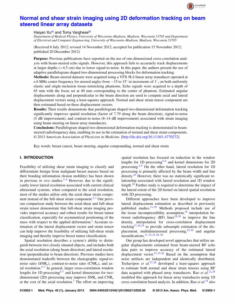
TABLE I. Mean and standard deviation of the strain stiffness contrast for the ellipsoidal inclusion TM phantoms for different angular increments for the 1D and2D deformation tracking approaches.

Angular increments

Phantom Modulus contrast Method 1◦ 3◦ 5◦ 15◦

Unbound ellipsoid (0◦/90◦) 4.2 1D Mean SSC 2.11 2.12 2.17 1.95Std 0.29 0.30 0.27 0.22

2D Mean SSC 2.11 2.08 2.09 2.08Std 0.04 0.03 0.03 0.06

Unbound ellipsoid (30◦/60◦) 3.2 1D Mean SSC 2.09 2.05 2.13 2.08Std 0.23 0.14 0.23 0.11

2D Mean SSC 2.11 2.07 2.07 2.00Std 0.09 0.11 0.11 0.12

Bound ellipsoid (0◦/90◦) 4.2 1D Mean SSC 2.07 2.14 2.06 1.88Std 0.18 0.18 0.20 0.30

2D Mean SSC 2.10 2.12 2.10 2.11Std 0.10 0.07 0.06 0.06

Bound ellipsoid (30◦/60◦) 3.2 1D Mean SSC 2.2 2.19 2.06 1.60Std 0.58 0.61 0.40 0.44

2D Mean SSC 1.96 1.96 1.96 1.93Std 0.03 0.05 0.04 0.07

Medical Physics, Vol. 40, No. 1, January 2013

012902-3 H. Xu and T. Varghese: 2D deformation tracking on beam steered linear array datasets 012902-3

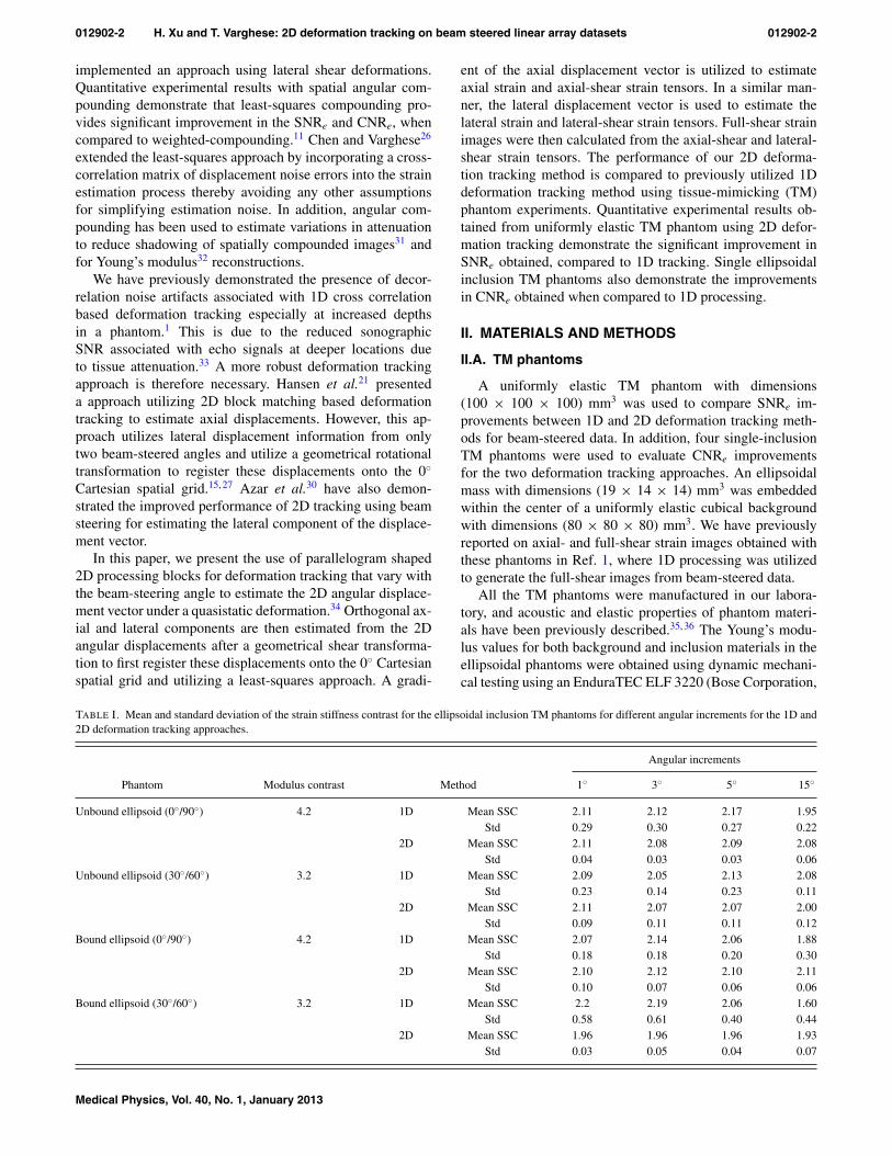
TABLE II. Mean and standard deviation of the strain stiffness contrast for the ellipsoidal inclusion TM phantoms for different maximum beam steered anglesfor the 1D and 2D deformation tracking approaches.

Maximum steered angle (◦)

Phantom Modulus contrast Method 3◦ 6◦ 9◦ 12◦ 15◦

Unbound ellipsoid (0◦/90◦) 4.2 1D Mean SSC 2.15 2.16 2.20 2.17 2.11Std 0.12 0.16 0.29 0.30 0.29

2D Mean SSC 2.12 2.13 2.12 2.11 2.11Std 0.05 0.04 0.05 0.05 0.04

Unbound ellipsoid (30◦/60◦) 3.2 1D Mean SSC 2.14 2.17 2.17 2.13 2.09Std 0.14 0.19 0.21 0.20 0.23

2D Mean SSC 2.06 2.05 2.05 2.06 2.11Std 0.11 0.10 0.10 0.10 0.09

Bound ellipsoid (0◦/90◦) 4.2 1D Mean SSC 2.01 2.10 2.13 2.27 2.07Std 0.25 0.25 0.21 0.60 0.18

2D Mean SSC 2.15 2.15 2.13 2.1 2.10Std 0.07 0.07 0.07 0.09 0.10

Bound ellipsoid (30◦/60◦) 3.2 1D Mean SSC 2.01 2.10 2.13 2.27 2.07Std 0.25 0.25 0.21 0.60 0.18

2D Mean SSC 2.15 2.15 2.13 2.11 2.10Std 0.07 0.07 0.07 0.09 0.10

EnduraTEC Systems Group, Minnetonka, MN) and has beenreported in Ref. 1. The contrast of each phantom was esti-mated from the ratio of Young’s modulus between the inclu-sion and background material as also shown in Tables I and II,respectively.

The ellipsoidal inclusion phantoms contained either abound inclusion (i.e., mass firmly attached to background ma-terial mimicking malignant breast masses) or an unbound in-clusion (i.e., mass loosely attached to the background mim-icking benign masses). The inclusion phantom pair eitherhad a symmetrical ellipsoidal inclusion oriented at 0◦/90◦, orasymmetrical inclusions oriented at 30◦/60◦ to the top sur-face of the phantom. Both the uniform and ellipsoidal inclu-sion phantoms were scanned using a Siemens S2000 real-timeclinical scanner (Siemens ultrasound, Mountain View, CA)equipped with a VFX 9L4 linear array transducer. The trans-ducer was operated at a 6 MHz center frequency, 80% band-width, and a sampling frequency of 40 MHz. Echo signalswere collected up to a depth of 65 mm with a single focusset at a depth of 40 mm, which also corresponds to the cen-ter of the four ellipsoidal inclusion phantoms. Beam-steeredRF data were acquired from −15◦ to 15◦ in increments of 1◦.Thus, 31 pairs of RF beam-steered data frames were acquiredbefore and after an applied deformation. Note that only a sin-gle deformation of 1% (1 or 0.8 mm) of the phantom heightwas applied to the phantom using a positioning stage. Thetransducer was embedded in a compressional plate larger thanthe TM phantom surface to provide a uniform deformationover the entire TM phantom surface.

II.B. Angular and displacement vector estimation

Angular displacement vectors (along and perpendicular tothe beam direction) at each beam steered angle (θ◦) were es-timated from the pre- and postdeformation echo signals us-

ing parallelogram shaped 2D cross correlation based displace-ment estimation. The parallelogram shaped kernel dimensionswas 0.385 mm along the beam direction ×3 RF-lines, with a75% overlap along beam direction and a lateral step of oneRF-line along its perpendicular direction. Note that the angu-lar displacement pairs were estimated from a Cartesian spatialgrid obtained for each beam steered angle.

In order to register angular displacements obtained foreach beam-steered angle, the estimated angular displacementvectors were first smoothed using spline interpolation alongeach beam-steered angle. The angular displacement vectorsfrom each angular Cartesian spatial grid were then transferredand registered into the Cartesian spatial grid obtained for the0◦ RF data. A geometrical shear transformation shown inEq. (1) was utilized to perform the transformation to the 0◦

Cartesian grid, shown as follows:

z = ztθ ,

x = tan(θ ) × ztθ + xtθ , (1)

where θ represents each beam-steering angle ranging from−15◦ to 15◦, ztθ and xtθ represent the axial and lateral co-ordinates of each beam steered Cartesian spatial grid, respec-tively, and z and x denote the axial and lateral coordinates ofthe 0◦ Cartesian spatial grid.

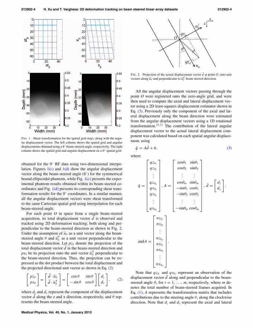
Comparisons between the Cartesian spatial grid obtainedfor 8◦ beam-steered data and its corresponding shear transfor-mation within the Cartesian spatial grid obtained along the 0◦

direction is shown in Figs. 1(a)–1(d), where (a) represents thespatial grid for the 8◦ beam-steered angle and (b) representsits corresponding shear geometrical transformation within thespatial grid for the 0◦ coordinate system. Note that a rectangu-lar spatial grid within the steered coordinates was transformedinto a parallelogram shape within the 0◦ coordinates. Basedon this spatial grid and shear transformation, both the angu-lar displacement vectors were transferred onto the spatial grid

Medical Physics, Vol. 40, No. 1, January 2013

012902-4 H. Xu and T. Varghese: 2D deformation tracking on beam steered linear array datasets 012902-4

FIG. 1. Shear transformation for the spatial grid (top), along with the angu-lar displacement vector. The left column shows the spatial grid and angulardisplacements obtained using a 8◦ beam-steered angle, respectively. The rightcolumn shows the spatial grid and angular displacement on a 0◦ spatial grid.

obtained for the 0◦ RF data using two-dimensional interpo-lation. Figures 1(c) and 1(d) show the angular displacementvector along the beam-steered angle (8◦) for the symmetricalbound ellipsoidal phantom, while Fig. 1(c) presents the exper-imental phantom results obtained within its beam-steered co-ordinates and Fig. 1(d) presents its corresponding shear trans-formation results for the 0◦ coordinates. In a similar manner,all the angular displacement vectors were shear transformedto the same Cartesian spatial grid using interpolation for eachbeam-steered angle.

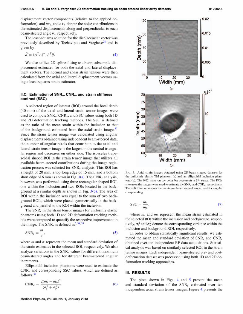
For each point O in space from a single beam-steeredacquisition, its total displacement vector �d is observed andtracked using 2D deformation tracking; both along and per-pendicular to the beam-steered direction as shown in Fig. 2.Under the assumption of uθ as a unit vector along the beam-steered angle θ and uT

θ as a unit vector perpendicular to thebeam-steered direction. Let pzθ denote the projection of thetotal displacement vector �d in the beam-steered direction andpxθ be its projection onto the unit vector uT

θ perpendicular tothe beam-steered direction. Thus, the projection can be ex-pressed as the dot product between the total displacement andthe projected directional unit vector as shown in Eq. (2)[

pzθ

pxθ

]=

[ �d · uθ

�d · uTθ

]=

[cos θ sin θ

− sin θ cos θ

] [dz

dx

], (2)

where dz and dx represent the component of the displacementvector �d along the z and x direction, respectively, and θ rep-resents the beam-steered angle.

FIG. 2. Projection of the actual displacement vector �d at point O, onto unitvectors along uθ and perpendicular to uT

θ beam steered direction.

All the angular displacement vectors passing through thepoint O were registered onto the zero-angle grid, and werethen used to compute the axial and lateral displacement vec-tor using a 2D least-squares displacement estimator shown inEq. (3). Previously only the component of the axial and lat-eral displacement along the beam direction were estimatedfrom the angular displacement vectors using a 1D rotationaltransformation.15, 21 The contribution of the lateral angulardisplacement vector to the actual lateral displacement com-ponent was calculated based on each spatial angular displace-ment, using

q̄ = Ad̄ + n̄, (3)

where

q̄ =

⎡⎢⎢⎢⎢⎢⎢⎢⎢⎢⎢⎢⎢⎢⎢⎢⎣

qzθ1

qzθ2

...

qzθm

qxθ1

qxθ2

...

qxθm

⎤⎥⎥⎥⎥⎥⎥⎥⎥⎥⎥⎥⎥⎥⎥⎥⎦

, A =

⎡⎢⎢⎢⎢⎢⎢⎢⎢⎢⎢⎢⎢⎢⎢⎢⎣

cosθ1 sinθ1

cosθ2 sinθ2

......

cosθm sinθm

−sinθ1 cosθ1

−sinθ2 cosθ2

......

−sinθm cosθm

⎤⎥⎥⎥⎥⎥⎥⎥⎥⎥⎥⎥⎥⎥⎥⎥⎦

, d̄ =[

dz

dx

],

and n̄ =

⎡⎢⎢⎢⎢⎢⎢⎢⎢⎢⎢⎢⎢⎢⎢⎢⎣

nzθ1

nzθ2

...

nzθm

nxθ1

nxθ2

...

nxθm

⎤⎥⎥⎥⎥⎥⎥⎥⎥⎥⎥⎥⎥⎥⎥⎥⎦

.

Note that qzθiand qxθi

represent an observation of thedisplacement vector d̄ along and perpendicular to the beam-steered angle θ i for i = 1, . . . , m, respectively, where m de-notes the total number of beam-steered frames acquired. InEq. (1), A represents the transformation matrix that includescontributions due to the steering angle θ i along the clockwisedirection. Note that dz and dx represent the axial and lateral

Medical Physics, Vol. 40, No. 1, January 2013

012902-5 H. Xu and T. Varghese: 2D deformation tracking on beam steered linear array datasets 012902-5

displacement vector components (relative to the applied de-formation), and nzθi

and nxθidenote the noise contributions in

the estimated displacements along and perpendicular to eachbeam-steered angle θ i, respectively.

The least-squares solution for the displacement vector waspreviously described by Techavipoo and Varghese28 and isgiven by

d̃ = (ATA)−1ATq̄. (4)

We also utilize 2D spline fitting to obtain subsample dis-placement estimates for both the axial and lateral displace-ment vectors. The normal and shear strain tensors were thencalculated from the axial and lateral displacement vectors us-ing a least-squares strain estimator.

II.C. Estimation of SNRe, CNRe, and strain stiffnesscontrast (SSC)

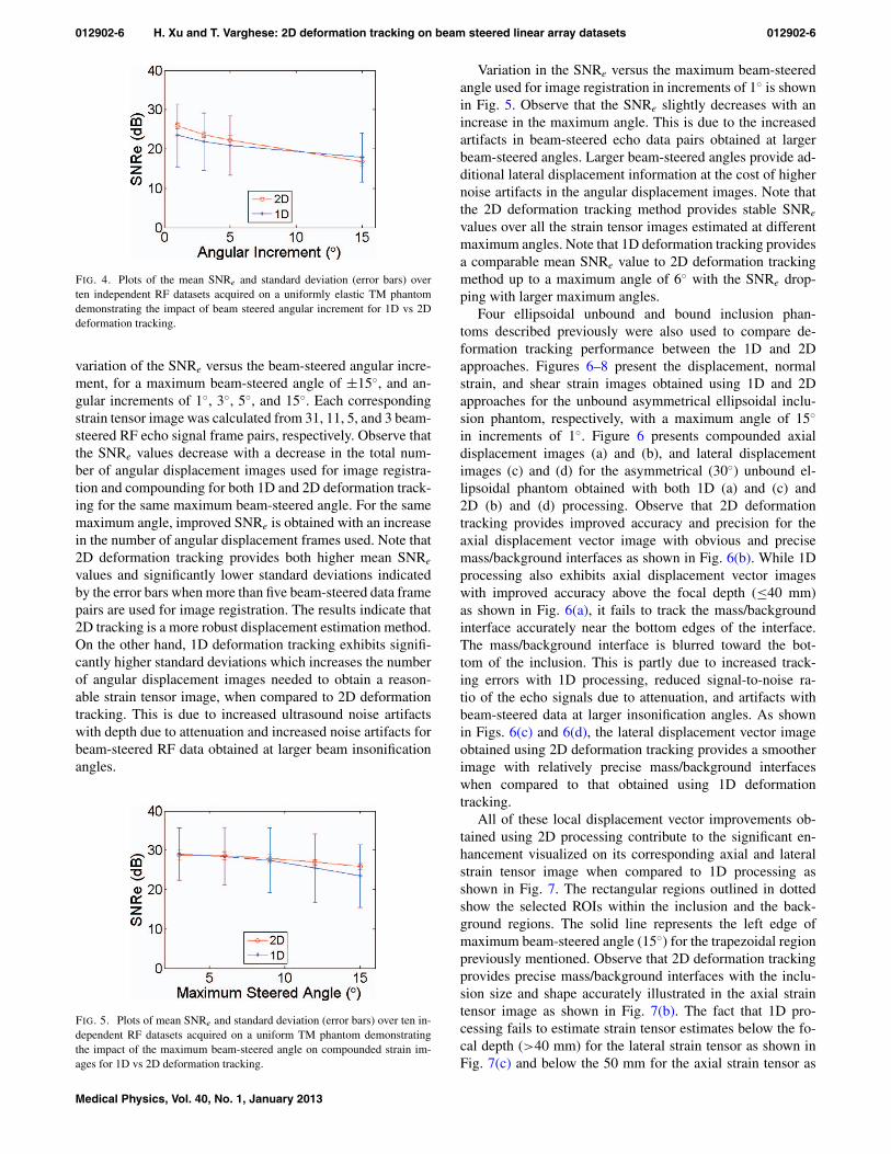
A selected region of interest (ROI) around the focal depth(40 mm) of the axial and lateral strain tensor images wereused to compute SNRe, CNRe, and SSC values using both 1Dand 2D deformation tracking methods. The SSC is definedas the ratio of the mean strain within the inclusion to thatof the background estimated from the axial strain image.37

Since the strain tensor image was calculated using angulardisplacements obtained using independent beam-steered data,the number of angular pixels that contribute to the axial andlateral strain tensor image is the largest in the central triangu-lar region and decreases on either side. The isosceles trape-zoidal shaped ROI in the strain tensor image that utilizes allavailable beam-steered contributions during the image regis-tration process was selected for SNRe analysis. This ROI hasa height of 20 mm, a top long edge of 15 mm, and a bottomshort edge of 6 mm as shown in Fig. 3(a). The CNRe analysis,however, was performed using three rectangular shaped ROI,one within the inclusion and two ROIs located in the back-ground at a similar depth as shown in Fig. 3(b). The area ofROI within the inclusion was equal to the sum of two back-ground ROIs, which were placed symmetrically in the back-ground and parallel to the ROI within the inclusion.

The SNRe in the strain tensor images for uniformly elasticphantoms using both 1D and 2D deformation tracking meth-ods were computed to quantify the respective improvement inthe image. The SNRe is defined as5, 38, 39

SNRe = m

σ, (5)

where m and σ represent the mean and standard deviation ofthe strain estimates in the selected ROI, respectively. We alsoanalyze variations in the SNRe values for different maximumbeam-steered angles and for different beam-steered angularincrements.

Ellipsoidal inclusion phantoms were used to estimate theCNRe and corresponding SSC values, which are defined asfollows:37

CNRe = 2(mi − mb)2

(σ 2i + σ 2

b ), (6)

FIG. 3. Axial strain images obtained using 2D beam steered datasets forthe uniformly elastic TM phantom (a) and an ellipsoidal inclusion phan-tom (b). The 0.02 value on the color bar represents a 2% strain. The ROIsshown on the images were used to estimate the SNRe and CNRe, respectively.The solid line represents the maximum beam steered angle used for angularcompounding.

SSC = mi

mb

, (7)

where mi and mb represent the mean strain estimated inthe selected ROI within the inclusion and background, respec-tively, σ 2

i and σ 2b denote the corresponding variance within the

inclusion and background ROI, respectively.In order to obtain statistically significant results, we esti-

mated the mean and standard deviation of SNRe and CNRe

obtained over ten independent RF data acquisitions. Statisti-cal analysis was based on similarly selected ROI in the straintensor images. Each independent beam-steered pre- and post-deformation dataset was processed using both 1D and 2D de-formation tracking approaches.

III. RESULTS

The plots shown in Figs. 4 and 5 present the meanand standard deviation of the SNRe estimated over tenindependent axial strain tensor images. Figure 4 presents the

Medical Physics, Vol. 40, No. 1, January 2013

012902-6 H. Xu and T. Varghese: 2D deformation tracking on beam steered linear array datasets 012902-6

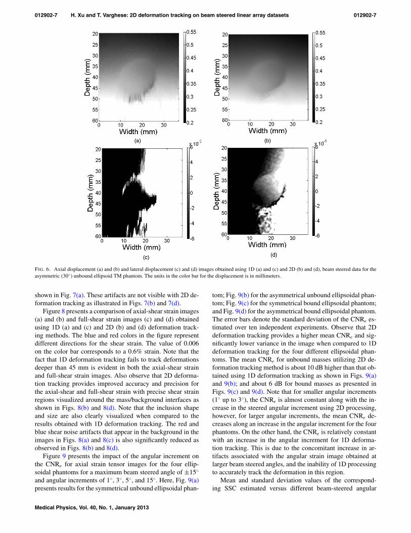
FIG. 4. Plots of the mean SNRe and standard deviation (error bars) overten independent RF datasets acquired on a uniformly elastic TM phantomdemonstrating the impact of beam steered angular increment for 1D vs 2Ddeformation tracking.

variation of the SNRe versus the beam-steered angular incre-ment, for a maximum beam-steered angle of ±15◦, and an-gular increments of 1◦, 3◦, 5◦, and 15◦. Each correspondingstrain tensor image was calculated from 31, 11, 5, and 3 beam-steered RF echo signal frame pairs, respectively. Observe thatthe SNRe values decrease with a decrease in the total num-ber of angular displacement images used for image registra-tion and compounding for both 1D and 2D deformation track-ing for the same maximum beam-steered angle. For the samemaximum angle, improved SNRe is obtained with an increasein the number of angular displacement frames used. Note that2D deformation tracking provides both higher mean SNRe

values and significantly lower standard deviations indicatedby the error bars when more than five beam-steered data framepairs are used for image registration. The results indicate that2D tracking is a more robust displacement estimation method.On the other hand, 1D deformation tracking exhibits signifi-cantly higher standard deviations which increases the numberof angular displacement images needed to obtain a reason-able strain tensor image, when compared to 2D deformationtracking. This is due to increased ultrasound noise artifactswith depth due to attenuation and increased noise artifacts forbeam-steered RF data obtained at larger beam insonificationangles.

FIG. 5. Plots of mean SNRe and standard deviation (error bars) over ten in-dependent RF datasets acquired on a uniform TM phantom demonstratingthe impact of the maximum beam-steered angle on compounded strain im-ages for 1D vs 2D deformation tracking.

Variation in the SNRe versus the maximum beam-steeredangle used for image registration in increments of 1◦ is shownin Fig. 5. Observe that the SNRe slightly decreases with anincrease in the maximum angle. This is due to the increasedartifacts in beam-steered echo data pairs obtained at largerbeam-steered angles. Larger beam-steered angles provide ad-ditional lateral displacement information at the cost of highernoise artifacts in the angular displacement images. Note thatthe 2D deformation tracking method provides stable SNRe

values over all the strain tensor images estimated at differentmaximum angles. Note that 1D deformation tracking providesa comparable mean SNRe value to 2D deformation trackingmethod up to a maximum angle of 6◦ with the SNRe drop-ping with larger maximum angles.

Four ellipsoidal unbound and bound inclusion phan-toms described previously were also used to compare de-formation tracking performance between the 1D and 2Dapproaches. Figures 6–8 present the displacement, normalstrain, and shear strain images obtained using 1D and 2Dapproaches for the unbound asymmetrical ellipsoidal inclu-sion phantom, respectively, with a maximum angle of 15◦

in increments of 1◦. Figure 6 presents compounded axialdisplacement images (a) and (b), and lateral displacementimages (c) and (d) for the asymmetrical (30◦) unbound el-lipsoidal phantom obtained with both 1D (a) and (c) and2D (b) and (d) processing. Observe that 2D deformationtracking provides improved accuracy and precision for theaxial displacement vector image with obvious and precisemass/background interfaces as shown in Fig. 6(b). While 1Dprocessing also exhibits axial displacement vector imageswith improved accuracy above the focal depth (≤40 mm)as shown in Fig. 6(a), it fails to track the mass/backgroundinterface accurately near the bottom edges of the interface.The mass/background interface is blurred toward the bot-tom of the inclusion. This is partly due to increased track-ing errors with 1D processing, reduced signal-to-noise ra-tio of the echo signals due to attenuation, and artifacts withbeam-steered data at larger insonification angles. As shownin Figs. 6(c) and 6(d), the lateral displacement vector imageobtained using 2D deformation tracking provides a smootherimage with relatively precise mass/background interfaceswhen compared to that obtained using 1D deformationtracking.

All of these local displacement vector improvements ob-tained using 2D processing contribute to the significant en-hancement visualized on its corresponding axial and lateralstrain tensor image when compared to 1D processing asshown in Fig. 7. The rectangular regions outlined in dottedshow the selected ROIs within the inclusion and the back-ground regions. The solid line represents the left edge ofmaximum beam-steered angle (15◦) for the trapezoidal regionpreviously mentioned. Observe that 2D deformation trackingprovides precise mass/background interfaces with the inclu-sion size and shape accurately illustrated in the axial straintensor image as shown in Fig. 7(b). The fact that 1D pro-cessing fails to estimate strain tensor estimates below the fo-cal depth (>40 mm) for the lateral strain tensor as shown inFig. 7(c) and below the 50 mm for the axial strain tensor as

Medical Physics, Vol. 40, No. 1, January 2013

012902-7 H. Xu and T. Varghese: 2D deformation tracking on beam steered linear array datasets 012902-7

FIG. 6. Axial displacement (a) and (b) and lateral displacement (c) and (d) images obtained using 1D (a) and (c) and 2D (b) and (d), beam steered data for theasymmetric (30◦) unbound ellipsoid TM phantom. The units in the color bar for the displacement is in millimeters.

shown in Fig. 7(a). These artifacts are not visible with 2D de-formation tracking as illustrated in Figs. 7(b) and 7(d).

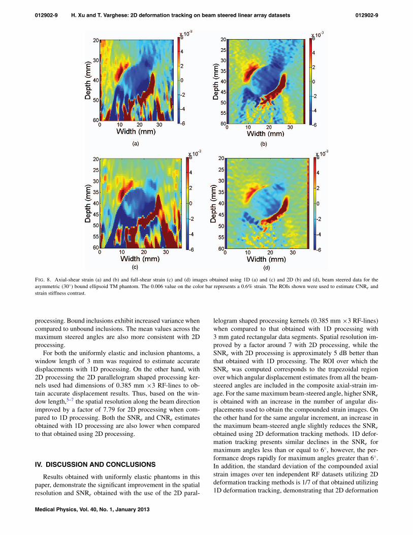
Figure 8 presents a comparison of axial-shear strain images(a) and (b) and full-shear strain images (c) and (d) obtainedusing 1D (a) and (c) and 2D (b) and (d) deformation track-ing methods. The blue and red colors in the figure representdifferent directions for the shear strain. The value of 0.006on the color bar corresponds to a 0.6% strain. Note that thefact that 1D deformation tracking fails to track deformationsdeeper than 45 mm is evident in both the axial-shear strainand full-shear strain images. Also observe that 2D deforma-tion tracking provides improved accuracy and precision forthe axial-shear and full-shear strain with precise shear strainregions visualized around the mass/background interfaces asshown in Figs. 8(b) and 8(d). Note that the inclusion shapeand size are also clearly visualized when compared to theresults obtained with 1D deformation tracking. The red andblue shear noise artifacts that appear in the background in theimages in Figs. 8(a) and 8(c) is also significantly reduced asobserved in Figs. 8(b) and 8(d).

Figure 9 presents the impact of the angular increment onthe CNRe for axial strain tensor images for the four ellip-soidal phantoms for a maximum beam steered angle of ±15◦

and angular increments of 1◦, 3◦, 5◦, and 15◦. Here, Fig. 9(a)presents results for the symmetrical unbound ellipsoidal phan-

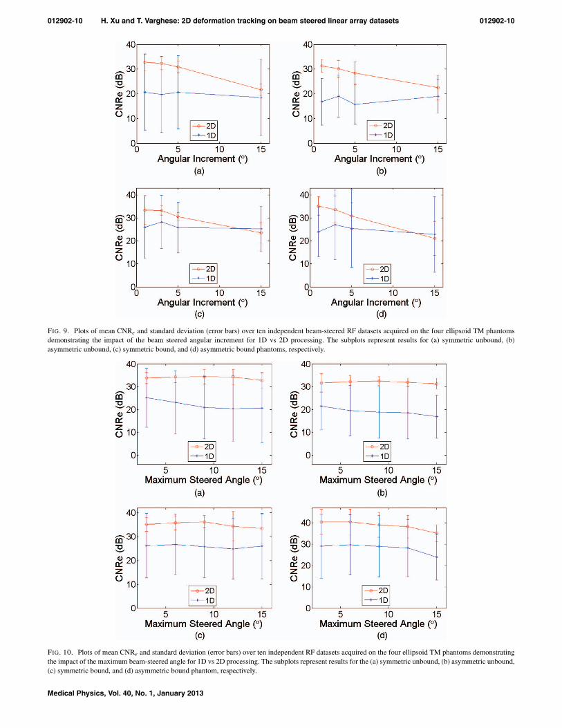
tom; Fig. 9(b) for the asymmetrical unbound ellipsoidal phan-tom; Fig. 9(c) for the symmetrical bound ellipsoidal phantom;and Fig. 9(d) for the asymmetrical bound ellipsoidal phantom.The error bars denote the standard deviation of the CNRe es-timated over ten independent experiments. Observe that 2Ddeformation tracking provides a higher mean CNRe and sig-nificantly lower variance in the image when compared to 1Ddeformation tracking for the four different ellipsoidal phan-toms. The mean CNRe for unbound masses utilizing 2D de-formation tracking method is about 10 dB higher than that ob-tained using 1D deformation tracking as shown in Figs. 9(a)and 9(b); and about 6 dB for bound masses as presented inFigs. 9(c) and 9(d). Note that for smaller angular increments(1◦ up to 3◦), the CNRe is almost constant along with the in-crease in the steered angular increment using 2D processing,however, for larger angular increments, the mean CNRe de-creases along an increase in the angular increment for the fourphantoms. On the other hand, the CNRe is relatively constantwith an increase in the angular increment for 1D deforma-tion tracking. This is due to the concomitant increase in ar-tifacts associated with the angular strain image obtained atlarger beam steered angles, and the inability of 1D processingto accurately track the deformation in this region.

Mean and standard deviation values of the correspond-ing SSC estimated versus different beam-steered angular

Medical Physics, Vol. 40, No. 1, January 2013

012902-8 H. Xu and T. Varghese: 2D deformation tracking on beam steered linear array datasets 012902-8

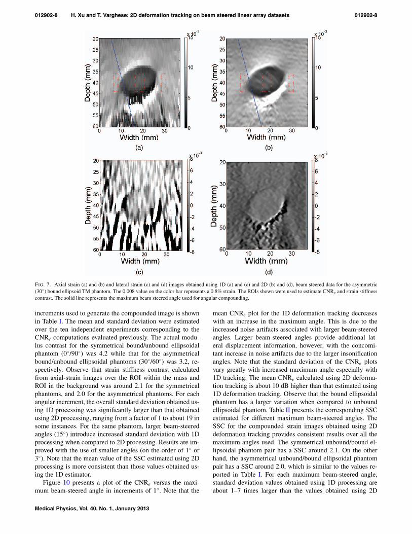
FIG. 7. Axial strain (a) and (b) and lateral strain (c) and (d) images obtained using 1D (a) and (c) and 2D (b) and (d), beam steered data for the asymmetric(30◦) bound ellipsoid TM phantom. The 0.008 value on the color bar represents a 0.8% strain. The ROIs shown were used to estimate CNRe and strain stiffnesscontrast. The solid line represents the maximum beam steered angle used for angular compounding.

increments used to generate the compounded image is shownin Table I. The mean and standard deviation were estimatedover the ten independent experiments corresponding to theCNRe computations evaluated previously. The actual modu-lus contrast for the symmetrical bound/unbound ellipsoidalphantom (0◦/90◦) was 4.2 while that for the asymmetricalbound/unbound ellipsoidal phantoms (30◦/60◦) was 3.2, re-spectively. Observe that strain stiffness contrast calculatedfrom axial-strain images over the ROI within the mass andROI in the background was around 2.1 for the symmetricalphantoms, and 2.0 for the asymmetrical phantoms. For eachangular increment, the overall standard deviation obtained us-ing 1D processing was significantly larger than that obtainedusing 2D processing, ranging from a factor of 1 to about 19 insome instances. For the same phantom, larger beam-steeredangles (15◦) introduce increased standard deviation with 1Dprocessing when compared to 2D processing. Results are im-proved with the use of smaller angles (on the order of 1◦ or3◦). Note that the mean value of the SSC estimated using 2Dprocessing is more consistent than those values obtained us-ing the 1D estimator.

Figure 10 presents a plot of the CNRe versus the maxi-mum beam-steered angle in increments of 1◦. Note that the

mean CNRe plot for the 1D deformation tracking decreaseswith an increase in the maximum angle. This is due to theincreased noise artifacts associated with larger beam-steeredangles. Larger beam-steered angles provide additional lat-eral displacement information, however, with the concomi-tant increase in noise artifacts due to the larger insonificationangles. Note that the standard deviation of the CNRe plotsvary greatly with increased maximum angle especially with1D tracking. The mean CNRe calculated using 2D deforma-tion tracking is about 10 dB higher than that estimated using1D deformation tracking. Observe that the bound ellipsoidalphantom has a larger variation when compared to unboundellipsoidal phantom. Table II presents the corresponding SSCestimated for different maximum beam-steered angles. TheSSC for the compounded strain images obtained using 2Ddeformation tracking provides consistent results over all themaximum angles used. The symmetrical unbound/bound el-lipsoidal phantom pair has a SSC around 2.1. On the otherhand, the asymmetrical unbound/bound ellipsoidal phantompair has a SSC around 2.0, which is similar to the values re-ported in Table I. For each maximum beam-steered angle,standard deviation values obtained using 1D processing areabout 1–7 times larger than the values obtained using 2D

Medical Physics, Vol. 40, No. 1, January 2013

012902-9 H. Xu and T. Varghese: 2D deformation tracking on beam steered linear array datasets 012902-9

FIG. 8. Axial-shear strain (a) and (b) and full-shear strain (c) and (d) images obtained using 1D (a) and (c) and 2D (b) and (d), beam steered data for theasymmetric (30◦) bound ellipsoid TM phantom. The 0.006 value on the color bar represents a 0.6% strain. The ROIs shown were used to estimate CNRe andstrain stiffness contrast.

processing. Bound inclusions exhibit increased variance whencompared to unbound inclusions. The mean values across themaximum steered angles are also more consistent with 2Dprocessing.

For both the uniformly elastic and inclusion phantoms, awindow length of 3 mm was required to estimate accuratedisplacements with 1D processing. On the other hand, with2D processing the 2D parallelogram shaped processing ker-nels used had dimensions of 0.385 mm ×3 RF-lines to ob-tain accurate displacement results. Thus, based on the win-dow length,5–7 the spatial resolution along the beam directionimproved by a factor of 7.79 for 2D processing when com-pared to 1D processing. Both the SNRe and CNRe estimatesobtained with 1D processing are also lower when comparedto that obtained using 2D processing.

IV. DISCUSSION AND CONCLUSIONS

Results obtained with uniformly elastic phantoms in thispaper, demonstrate the significant improvement in the spatialresolution and SNRe obtained with the use of the 2D paral-

lelogram shaped processing kernels (0.385 mm ×3 RF-lines)when compared to that obtained with 1D processing with3 mm gated rectangular data segments. Spatial resolution im-proved by a factor around 7 with 2D processing, while theSNRe with 2D processing is approximately 5 dB better thanthat obtained with 1D processing. The ROI over which theSNRe was computed corresponds to the trapezoidal regionover which angular displacement estimates from all the beam-steered angles are included in the composite axial-strain im-age. For the same maximum beam-steered angle, higher SNRe

is obtained with an increase in the number of angular dis-placements used to obtain the compounded strain images. Onthe other hand for the same angular increment, an increase inthe maximum beam-steered angle slightly reduces the SNRe

obtained using 2D deformation tracking methods. 1D defor-mation tracking presents similar declines in the SNRe formaximum angles less than or equal to 6◦, however, the per-formance drops rapidly for maximum angles greater than 6◦.In addition, the standard deviation of the compounded axialstrain images over ten independent RF datasets utilizing 2Ddeformation tracking methods is 1/7 of that obtained utilizing1D deformation tracking, demonstrating that 2D deformation

Medical Physics, Vol. 40, No. 1, January 2013

012902-10 H. Xu and T. Varghese: 2D deformation tracking on beam steered linear array datasets 012902-10

FIG. 9. Plots of mean CNRe and standard deviation (error bars) over ten independent beam-steered RF datasets acquired on the four ellipsoid TM phantomsdemonstrating the impact of the beam steered angular increment for 1D vs 2D processing. The subplots represent results for (a) symmetric unbound, (b)asymmetric unbound, (c) symmetric bound, and (d) asymmetric bound phantoms, respectively.

FIG. 10. Plots of mean CNRe and standard deviation (error bars) over ten independent RF datasets acquired on the four ellipsoid TM phantoms demonstratingthe impact of the maximum beam-steered angle for 1D vs 2D processing. The subplots represent results for the (a) symmetric unbound, (b) asymmetric unbound,(c) symmetric bound, and (d) asymmetric bound phantom, respectively.

Medical Physics, Vol. 40, No. 1, January 2013

012902-11 H. Xu and T. Varghese: 2D deformation tracking on beam steered linear array datasets 012902-11

FIG. 11. Plots of mean SNRe and standard deviation (error bars) over ten independent RF datasets acquired on an uniformly elastic TM phantom demonstratingthe impact of different maximum angles on similar number of compounded strain images. Results are shown for 3 beam steered angles (a), 5 beam-steered angles(b), 7 beam-steered angles (c), and 11 beam-steered angles (d), respectively.

tracking is both an accurate and robust deformation trackingmethod.

Noise artifacts observed below the inclusion with 1D pro-cessing were not visible with 2D processing for displacement,strain and shear strain images, demonstrating the superior de-formation tracking obtained with 2D tracking, especially forregions with lower signal-to-noise. Lateral strain images thatwere poorly tracked using the 1D deformation tracking ap-proach are significantly improved with 2D processing. In ad-dition, 2D deformation tracking provides clear and smoothinclusion/background interfaces over the entire image, wherethese interfaces clearly differentiate the inclusions for bothunbound and bound masses. Asymmetrical inclusion phan-toms poorly tracked with 1D processing are clearly visualizedwith 2D processing. Background noise artifacts in strain im-ages observed with 1D processing were significantly reducedusing 2D processing.

Experimental results for the ellipsoidal phantoms showthat the 2D parallelogram shaped processing blocks for de-formation tracking provide a significant improvement in theCNRe of 14 dB for unbound masses and 8 dB for boundmasses, respectively, for a maximum angle of 15◦, when com-pared to results obtained using 1D deformation tracking. TheCNRe curves presented in Fig. 9 exhibit saturation for smallerangular increments, which corresponds to results presented inRef. 11. For smaller angular increments, the angular displace-ments obtained are highly correlated, and an angular incre-

ment of approximately 3◦ is enough to obtain accurate com-pounded strain images using either 1D or 2D deformationtracking methods. Since the error bars for 1D processing aresignificantly larger than those for 2D processing, there is someoverlap between the error bars for the two methods. However,note the length of the error bars for 2D processing when com-pared to 1D deformation tracking, which partly indicates therobustness of the 2D deformation tracking approach describedin this paper.

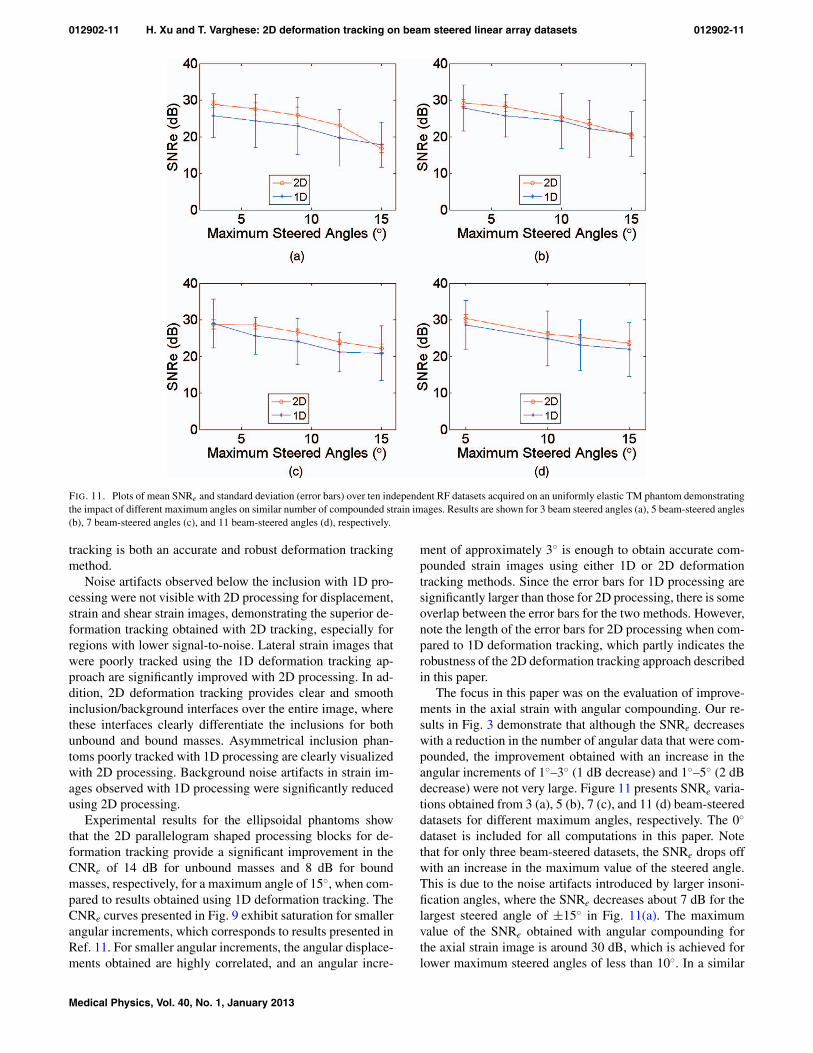
The focus in this paper was on the evaluation of improve-ments in the axial strain with angular compounding. Our re-sults in Fig. 3 demonstrate that although the SNRe decreaseswith a reduction in the number of angular data that were com-pounded, the improvement obtained with an increase in theangular increments of 1◦–3◦ (1 dB decrease) and 1◦–5◦ (2 dBdecrease) were not very large. Figure 11 presents SNRe varia-tions obtained from 3 (a), 5 (b), 7 (c), and 11 (d) beam-steereddatasets for different maximum angles, respectively. The 0◦

dataset is included for all computations in this paper. Notethat for only three beam-steered datasets, the SNRe drops offwith an increase in the maximum value of the steered angle.This is due to the noise artifacts introduced by larger insoni-fication angles, where the SNRe decreases about 7 dB for thelargest steered angle of ±15◦ in Fig. 11(a). The maximumvalue of the SNRe obtained with angular compounding forthe axial strain image is around 30 dB, which is achieved forlower maximum steered angles of less than 10◦. In a similar

Medical Physics, Vol. 40, No. 1, January 2013

012902-12 H. Xu and T. Varghese: 2D deformation tracking on beam steered linear array datasets 012902-12

manner in Fig. 9, smaller angular increments on the order of1◦–3◦, also provide similar CNRe results. For a maximum an-gle of 15◦, 11 beam-steered datasets at 3◦ increments providesimilar performance as 31 beam-steered datasets at 1◦ angu-lar increments. In general, an optimal number of beam-steereddatasets would be the most appropriate for a given maximumvalue of the beam-steered angle. However, it is difficult to de-termine a generic value of an optimum angular increment andmaximum angle as it would also depend on the transducercenter frequency, bandwidth, and array transducer construc-tion parameters that would determine side-lobes and gratinglobes. In general, from our results for the system and trans-ducer utilized, the SNRe and CNRe are maximized for angularincrements around 3◦ and maximum angles less than 10◦.

Several investigators have also reported on the use of onlythree beam-steered datasets to estimate both axial and lat-eral displacement vectors and strain tensors.21, 30 The premiseemployed by these investigators is that the 0◦ dataset wouldprovide axial strain information, while the beam-steered dataacquired at the largest possible steered angle could be uti-lized for lateral strain computation by estimation of the lat-eral components along the beam-steered data. Larger beam-steered angles provide more lateral deformation informationat the cost of introducing additional noise artifacts into boththe strain tensor images. Larger steered angles improve lat-eral strain estimation, however, the impact of grating lobesand other noise artifacts have to be considered especially forlinear array transducers. However, these larger beam-steeredangles also significantly reduce both the SNRe and CNRe inthe axial strain images as illustrated in Fig. 11(a) for the threedatasets obtained at the 0◦ and ±15◦ angular increments.

The discussion in the above two paragraphs demonstratesthe opposing and competing requirements if one attempts tomaximize the SNRe and CNRe in both the axial and lateralstrain tensors utilizing the same beam-steered datasets. Max-imizing the SNRe and CNRe for axial strain imaging requiressmaller angular increments and lower maximum steered an-gles as illustrated in this paper. On the other hand, accuratelateral strain imaging require larger beam-steered angles.15, 21

Several tradeoffs therefore have to be considered, if oneproposes to minimize the number of beam-steered anglesfor clinical applications. If the temporal resolution is impor-tant, for example, for imaging moving structures fewer anglesshould be utilized. On the other hand, if the spatial resolu-tion and improvement in the SNRe and CNRe is the decid-ing parameter, more beam-steered datasets can be included inthe computation to maximize the SNRe and CNRe obtained.Computational aspects with beam steering have also to beconsidered for clinical applications. In our implementation,beam-steered data acquisition was inefficient since it was per-formed using a script on a laptop to control the data acqui-sition. Processing of the beam-steered RF datasets was alsoperformed using MATLAB. Computationally efficient imple-mentations of both 1D and 2D processing exist that wouldenable us to obtain angular displacements in real-time. How-ever, reductions in the frame-rate for strain imaging will defi-nitely occur with the use of a larger number of steered anglesfor angular compounding. In addition, beam steering, data ac-

quisition, and processing have to be implemented on the ul-trasound system to further improve computational efficiency.

ACKNOWLEDGMENTS

This work was supported by Komen Grant No.BCTR0601153 and National Institutes of Health (NIH)-Cancer Institute (NCI) Grant Nos. 5R21CA140939-02,R01CA112192-S103, and R01CA112192-05.

a)Electronic mail: hxu26@wisc.edub)Author to whom correspondence should be addressed. Electronic mail:

tvarghese@wisc.edu; Telephone: (608) 265-8797; Fax: (608) 262-2413.1H. Xu, T. Varghese, and E. L. Madsen, “Analysis of shear strain imagingfor classifying breast masses: Finite element and phantom results,” Med.Phys. 38, 6119–6127 (2011).

2H. Xu, M. Rao, T. Varghese, S. Baker, A. M. Sommer, T. J. Hall, E. S. Burn-side, and G. A. Sisney, “Axial-shear strain imaging for differentiating be-nign and malignant breast masses,” Ultrasound Med. Biol. 36, 1813–1824(2010).

3A. Thitaikumar, L. M. Mobbs, C. M. Kraemer-Chant, B. S. Garra, andJ. Ophir, “Breast tumor classification using axial shear strain elastography:A feasibility study,” Phys. Med. Biol. 53, 4809–4823 (2008).

4E. E. Konofagou, T. Harrigan, and J. Ophir, “Shear strain estimation and le-sion mobility assessment in elastography,” Ultrasonics 38, 400–404 (2000).

5T. Varghese, M. Bilgen, and J. Ophir, “Multiresolution imaging in elastog-raphy,” IEEE Trans. Ultrason. Ferroelectr. Freq. Control 45, 65–75 (1998).

6R. Righetti, J. Ophir, and P. Ktonas, “Axial resolution in elastography,”Ultrasound Med. Biol. 28, 101–113 (2002).

7S. Srinivasan, R. Righetti, and J. Ophir, “Trade-offs between the axial reso-lution and the signal-to-noise ratio in elastography,” Ultrasound Med. Biol.29, 847–866 (2003).

8H. Chen, H. Shi, and T. Varghese, “Improvement of elastographic displace-ment estimation using a two-step cross-correlation method,” UltrasoundMed. Biol. 33, 48–56 (2007).

9Y. Zhu and T. Hall, “A modified block matching method for real-time free-hand strain imaging,” Ultrason. Imaging 24, 161–176 (2002).

10R. Righetti, S. Srinivasan, and J. Ophir, “Lateral resolution in elastogra-phy,” Ultrasound Med. Biol. 29, 695–704 (2003).

11M. Rao and T. Varghese, “Spatial angular compounding for elastographywithout the incompressibility assumption,” Ultrason. Imaging 27, 256–270(2005).

12M. Rao, Q. Chen, H. Shi, and T. Varghese, “Spatial-angular compoundingfor elastography using beam steering on linear array transducers,” Med.Phys. 33, 618–626 (2006).

13M. Rao, Q. Chen, H. Shi, T. Varghese, E. L. Madsen, J. A. Zagzebski,and T. Wilson, “Normal and shear strain estimation using beam steering onlinear-array transducers,” Ultrasound Med. Biol. 33, 57–66 (2007).

14M. Rao, T. Varghese, and E. L. Madsen, “Shear strain imaging using sheardeformations,” Med. Phys. 35, 412–423 (2008).

15U. Techavipoo, Q. Chen, T. Varghese, and J. A. Zagzebski, “Estimationof displacement vectors and strain tensors in elastography using angularinsonifications,” IEEE Trans. Med. Imaging 23, 1479–1489 (2004).

16M. A. Lubinski, S. Y. Emelianov, K. R. Raghavan, A. E. Yagle,A. R. Skovoroda, and M. O’Donnell, “Lateral displacement estimation us-ing tissue incompressibility,” IEEE Trans. Ultrason. Ferroelectr. Freq. Con-trol 43, 247–256 (1996).

17I. Cespedes, Y. Huang, J. Ophir, and S. Spratt, “Methods for estimation ofsubsample time delays of digitized echo signals,” Ultrason. Imaging 17,142–171 (1995).

18F. Viola and W. F. Walker, “A spline-based algorithm for continuous time-delay estimation using sampled data,” IEEE Trans. Ultrason. Ferroelectr.Freq. Control 52, 80–93 (2005).

19E. Konofagou and J. Ophir, “A new elastographic method for estimationand imaging of lateral displacements, lateral strains, corrected axial strainsand Poisson’s ratios in tissues,” Ultrasound Med. Biol. 24, 1183–1199(1998).

20J. Luo and E. E. Konofagou, “Effects of various parameters on lateral dis-placement estimation in ultrasound elastography,” Ultrasound Med. Biol.35, 1352–1366 (2009).

Medical Physics, Vol. 40, No. 1, January 2013

012902-13 H. Xu and T. Varghese: 2D deformation tracking on beam steered linear array datasets 012902-13

21H. H. Hansen, R. G. Lopata, T. Idzenga, and C. L. de Korte, “Full 2Ddisplacement vector and strain tensor estimation for superficial tissue us-ing beam-steered ultrasound imaging,” Phys. Med. Biol. 55, 3201–3218(2010).

22S. Korukonda and M. M. Doyley, “Estimating axial and lateral strain usinga synthetic aperture elastographic imaging system,” Ultrasound Med. Biol.37, 1893–1908 (2011).

23R. G. Lopata, M. M. Nillesen, H. H. Hansen, I. H. Gerrits, J. M. Thi-jssen, and C. L. de Korte, “Performance evaluation of methods for two-dimensional displacement and strain estimation using ultrasound radio fre-quency data,” Ultrasound Med. Biol. 35, 796–812 (2009).

24F. Viola, R. L. Coe, K. Owen, D. A. Guenther, and W. F. Walker, “Multi-dimensional spline-based estimator (MUSE) for motion estimation: algo-rithm development and initial results,” Ann. Biomed. Eng. 36, 1942–1960(2008).

25R. Z. Azar, O. Goksel, and S. E. Salcudean, “Sub-sample displacementestimation from digitized ultrasound RF signals using multi-dimensionalpolynomial fitting of the cross-correlation function,” IEEE Trans. Ultrason.Ferroelectr. Freq. Control 57, 2403–2420 (2010).

26Q. Chen, A. L. Gerig, U. Techavipoo, J. A. Zagzebski, and T. Varghese,“Correlation of RF signals during angular compounding,” IEEE Trans. Ul-trason. Ferroelectr. Freq. Control 52, 961–970 (2005).

27U. Techavipoo, Q. Chen, T. Varghese, J. A. Zagzebski, and E. L. Mad-sen, “Noise reduction using spatial-angular compounding for elastogra-phy,” IEEE Trans. Ultrason. Ferroelectr. Freq. Control 51, 510–520 (2004).

28U. Techavipoo and T. Varghese, “Improvements in elastographic contrast-to-noise ratio using spatial-angular compounding,” Ultrasound Med. Biol.31, 529–536 (2005).

29M. Rao and T. Varghese, “Correlation analysis for angular compoundingin strain imaging,” IEEE Trans. Ultrason. Ferroelectr. Freq. Control 54,1903–1907 (2007).

30R. Z. Azar, O. Goksel, and S. Salcudean, “Comparison between 2-Dcross correlation with 2-D sub-sampling and 2-D tracking using beamsteering,” IEEE Trans. Ultrason. Ferroelectr. Freq. Control 58, 1534–1537(2011).

31G. M. Treece, A. H. Gee, and R. W. Prager, “Ultrasound compounding withautomatic attenuation compensation using paired angle scans,” UltrasoundMed. Biol. 33, 630–642 (2007).

32R. Z. Azar, A. Baghani, S. E. Salcudean, and R. Rohling, “2-D high-frame-rate dynamic elastography using delay compensatedand angularly compounded motion vectors: Preliminary results,”IEEE Trans. Ultrason. Ferroelectr. Freq. Control 57, 2421–2436(2010).

33T. Varghese and J. Ophir, “The nonstationary strain filter in elastography:Part I. Frequency dependent attenuation,” Ultrasound Med. Biol. 23, 1343–1356 (1997).

34T. Varghese, “Quasi-static ultrasound elastography,” Ultrasound Clin. 4,323–338 (2009).

35E. L. Madsen, M. A. Hobson, H. Shi, T. Varghese, and G. R. Frank, “Sta-bility of heterogeneous elastography phantoms made from oil dispersionsin aqueous gels,” Ultrasound Med. Biol. 32, 261–270 (2006).

36E. L. Madsen, M. A. Hobson, G. Frank, H. Shi, J. Jiang, T. J. Hall, T. Vargh-ese, M. M. Doyley, and J. B. Weaver, “Anthropomorphic breast phan-toms for testing elastography systems,” Ultrasound Med. Biol. 32, 857–874(2006).

37T. Varghese and J. Ophir, “An analysis of elastographic contrast-to-noiseratio,” Ultrasound Med. Biol. 24, 915–924 (1998).

38I. Cespedes and J. Ophir, “Reduction of image noise in elastography,”Ultrason. Imaging 15, 89–102 (1993).

39T. Varghese and J. Ophir, “A theoretical framework for performance char-acterization of elastography: The strain filter,” IEEE Trans. Ultrason. Fer-roelectr. Freq. Control 44, 164–172 (1997).

Medical Physics, Vol. 40, No. 1, January 2013