Embed Size (px)
Citation preview

too poor to be efficient? impacts of the targetedfertilizer subsidy programme in malawi on farmplot level input use, crop choice and land productivity
by Stein holden and rodney lunduka
No
ragric Report N
o. 55
Departm
ent o
f Intern
ation
al Enviro
nm
ent an
d D
evelopm
ent S
tud
iesN
orag
ric

TOO POOR TO BE EFFICIENT?
IMPACTS OF THE TARGETED FERTILIZER SUBSIDY PROGRAMME IN MALAWI ON FARM PLOT LEVEL INPUT USE, CROP CHOICE AND
LAND PRODUCTIVITY
By Stein Holden and Rodney Lunduka
Noragric Report No. 55 September 2010
Department of International Environment and Development Studies, Noragric
Norwegian University of Life Sciences, UMB

ii
Noragric is the Department of International Environment and Development Studies at the Norwegian University of Life Sciences (UMB). Noragric’s activities include research, education and assignments, focusing particularly, but not exclusively, on developing countries and countries with economies in transition. Noragric Reports present findings from various studies and assignments, including programme appraisals and evaluations. This Noragric Report was commissioned by the Norwegian Agency for Development Cooperation (Norad) under the framework agreement with UMB which is administrated by Noragric. Extracts from this publication may only be reproduced after prior consultation with the employer of the assignment (Norad) and with the consultant team leader (Noragric). This Report (May 2010) is written by the UMB Department of Economics and Resource Management. The authors wish to thank NORAD for financial support of this project and a group of Master students in the NOMA Development and Natural Resource Economics programme for their efforts in data collection. The findings, interpretations and conclusions expressed in this publication are entirely those of the authors and cannot be attributed directly to the Department of International Environment and Development Studies (UMB/Noragric).
Holden, Stein1
Noragric Report No. 55 (September 2010).
and Rodney Lunduka. Too poor to be efficient? Impacts of the targeted fertilizer subsidy programme in Malawi on farm plot level input use, crop choice and land productivity.
Department of International Environment and Development Studies, Noragric Norwegian University of Life Sciences (UMB) P.O. Box 5003 N-1432 Aas Norway Tel.: +47 64 96 52 00 Fax: +47 64 96 52 01 Internet: http://www.umb.no/noragric ISSN: 1502-8127 Photo credits: Josie Teurlings (cover) Cover design: Åslaug Borgan/UMB Printed at: Elanders Novum 1 Department of Economics and Resource Management, Norwegian University of Life Sciences, P. O. Box 5033, 1432 Ås, Norway. Email: [email protected]

iii
TABLE OF CONTENTS INTRODUCTION 1 1. DATA AND METHODS OF ANALYSIS 2 1.1. Data 2 1.2. Assessing the impact of the subsidy programme 3 1.3. Asset poverty categorization of households 4 1.3.1. Econometric methods 4 2. RESULTS AND DISCUSSION 5 2.1. Household farm plot level decisions on fertilizer and manure use 5 2.2. Fertilizer and manure demand intensity at farm plot level 9 2.3. Land productivity on maize plots, the effects of improved seeds and fertilizer use intensity 15 2.4. Asset poverty, plot level application of subsidized fertilizers and maize productivity 22 2.4.1. Factors associated with farm plot level crop choice 25 2.4.2. Factors associated with farm level maize area, maize area per capita and maize area share 28 2.4.3. Intercropping pattern 35 2.5. Trees on farm plots: Are there any effects of the subsidy programme? 39 CONCLUSION 44 APPENDIX 48

Dept. of International Environment and Development Studies, Noragric
1
INTRODUCTION Malawi has over the last four years embarked on a comprehensive fertilizer and seed subsidy programme to boost its agricultural production and to enhance food security in the country. The programme aims to provide coupons for purchase of subsidized fertilizer and seeds to targeted poor rural households. It is of high interest to know more about the efficiency of the fertilizer-seed targeting programme in reaching poor households, the productivity and food security impacts of the subsidized fertilizers and seeds, the interaction effects of fertilizers and seeds, and whether fertilizer subsidies crowd out organic manures and other crops than maize. The objectives of this study are to identify
1) The extent to which the targeted fertilizer and seed subsidy programme results in efficient utilization of these inputs through enhancement of farm plot level land productivity,
2) The productivity of alternative seed varieties of maize (hybrid varieties (HYVs) and open-pollinated varieties (OPVs) versus local seeds),
3) The extent to which fertilizer subsidies for maize crowd out other crops and the use of organic manures and have other sustainable land management implications.
The report sets out to try to provide answers to a substantial number of research questions:
1. Is the plot level probability of fertilizer application enhanced by access to subsidies? 2. How is the probability of fertilizer application correlated with the probability of manure
application? Does fertilizer application crowd in or crowd out manure application at farm plot level?
3. Are manure and fertilizer used as substitutes or complements and does this differ for maize plots versus on all crops?
4. What is the interaction effect between fertilizer and manure on maize productivity? 5. Does access to fertilizer subsidies enhance maize land productivity after controlling for
endogeneity in allocation of subsidies? 6. Are those getting fertilizer subsidies as efficient as those not getting fertilizer subsidies in
terms of maize land productivity? 7. How productive are households that should have been targeted by the subsidy (poverty
targeting) but failed to be reached (errors of exclusion), as compared to those that should not have been reached and did not receive fertilizer subsidies?
8. How productive are households that should not have been targeted but received subsidies (errors of exclusion) as compared to those that should have been targeted and received subsidies?
9. Is access to improved maize varieties enhancing fertilizer use intensity? If yes, how much?
10. Is maize land productivity higher for improved maize varieties (HYVs and OPVs) after controlling for differences in fertilizer use intensity? If yes, how much?
11. Is maize productivity improving over time? 12. How is maize productivity associated with asset poverty?

Dept. of International Environment and Development Studies, Noragric
2
13. Does access to fertilizer subsidies crowd out other crops and lead to increasing area under maize or does it lead to intensification of maize production and reduced area share of maize?
14. How is crop choice associated with asset poverty and access to fertilizer subsidies? 15. Does more use of fertilizers crowd out intercrops and lead to more mono-cropping of
maize? 16. How has access to subsidies affected household plot level investments in tree planting
and removal of natural trees? 17.
This study used the data from initially 450 households and their farm plots in six districts (Thyolo, Chiradzulu, Zomba, Machinga, Lilongwe and Kasungu) in central and southern Malawi for the years 2006, 2007 and 2009. Due to attrition the sample was reduced to 378 households in 2009. As the report attempts to cover a lot of “ground” the presentation is brief and not very elaborate to avoid that the report becomes too long. There are certainly a lot of issues that are touched upon that deserve a more elaborate discussion. Hopefully some of these emerge in more elaborate and narrowly focused papers in the future, also linking the findings up to the research literature, which this report does not do. 1. DATA AND METHODS OF ANALYSIS 1.1. DATA The Norwegian University of Life Sciences’ Department of Economics and Resource Management is running a NORAD-funded (NOMA) collaborative MSc-programme in Development and Natural Resource Economics together with four African Universities. University of Malawi, Bunda College of Agriculture, has been the host for the students during the spring 2009 and the students carried out fieldwork for their MSc-theses during June and July 2009 in Malawi. This was a follow-up survey to 450 households in six districts in Central and Southern Malawi and was the third round survey to the same households. The earlier rounds were in 2006 and 2007. Only 378 of these households were found and interviewed in this new survey round. This gives a three round unbalanced panel of household and plot level data that can be used to assess the impacts of the fertilizer subsidy programme. The household and plot panel nature of the data allow us to control for observable and unobservable household and farm plot characteristics by using household random and fixed effects models. An attribute of the survey, which is different from some other surveys in Malawi, is that we collected information on all plots of the households. The farm plot level data collection included visiting and measuring each plot with a GPS. Plot sizes should therefore be fairly reliable and much more reliable than if one had to rely on households’ own estimates of plot sizes. Still, plot size was included as a right hand side variable

Dept. of International Environment and Development Studies, Noragric
3
in models where output or input per unit land was included as a dependent variable, in order to correct for measurement error. 1.2. ASSESSING THE IMPACT OF THE SUBSIDY PROGRAMME We included a dummy variable for whether households have received subsidies or not in each of the years. The problem with this subsidy variable is that it is endogenous. We have therefore also run a model to predict access to subsidized fertilizer. We used an unconventional approach for this which briefly may be explained as follows: We used a linear probability model with household fixed effects and used it to predict the likelihood of households receiving subsidized (coupon) fertilizer (including the unobserved household effect in the prediction). We derived four categories of observations for households:
a) Hhsubsidy01: Have not received subsidy but was predicted to get b) Hhsubsidy11: Received subsidy and was predicted to get (used as “baseline”) c) Hhsubsidy10: Received subsidy and was not predicted to get d) Hhsubsidy00: Did not receive subsidy and was not predicted to get.
With clear targeting criteria based on household characteristics these four variables should capture errors of exclusion and errors of inclusion and we may expect systematic differences between these four groups and these differences may also have implications for the impacts. With unclear targeting criteria that vary across communities and years it is possible that such differences will be insignificant. The problem is that we do not know for sure why some are more successful and others less successful in obtaining the coupons although we get some insights by using observable household characteristics and see how they are correlated with accessing coupons. We can say it is determined partly by unobservable household characteristics which may be related to their social networks, position, influence, kinship ties, and information available and decisions made by those responsible for the targeting. These factors may be different from the official targeting criteria which are poverty, vulnerability etc. The method used is pragmatic about what causes some households to be recipients and others not as it “mines the data” including unobservable household characteristics (captured by household dummy variables) to identify who were successful. Based on this we predict the probability of households getting subsidies in each year. “Errors of exclusion” then are those that are predicted (with probability higher than 50%) to receive but not having received a coupon. Similarly, household predicted not to get (probability less than 50%) but receiving are “errors of inclusion” based on the actual pattern of distribution. The method allows different mechanisms to be at work in the distribution in each community. For example, a household that received coupons in 2 out of 3 years is more likely to be predicted as a recipient than one household that received coupons in only one or none of the years. Based on the “local standard” established over three years, the household that received coupons in two years is representing an “error of exclusion” in the third year when it did not receive, if it is predicted to receive with a probability higher than 0.5 in the year it did not receive. A simple approach to assessing the impact of the programme would be to measure:

Dept. of International Environment and Development Studies, Noragric
4
i) Hhsubsidy11 – Hhsubsidy01: Impact of access for household predicted to receive subsidy ii) Hhsubsidy10 – Hhsubsidy00: Impact of access for households predicted not to receive
subsidy This relies on the assumption that the approach allows us to remove differences due to unobserved heterogeneity. The same approach was also used to predict use of subsidized fertilizer at the farm plot level while also including observable plot characteristics while unobservable time-invariant plot characteristics were controlled for with household fixed effects. Finally, the same approach was used to predict the plot level use of hybrid maize seeds. 1.3. ASSET POVERTY CATEGORIZATION OF HOUSEHOLDS
In order to assess how household poverty both was related to access to subsidies and affected maize productivity, households were categorized based on their possession of basic resources and assets per capita. This was done within each year for the three year panel. Within each year households that fell below the median level of that specific resource or asset in per capita terms was classified as poor in that resource. The classification is therefore a relative classification related to the other households in the random sample of households. The classification was done for the following resources/endowments; land endowment per capita; labour endowment per capita; livestock endowment per capita (measured in tropical livestock units); and real value of assets per capita. Models of three types were then developed:
a) Models with asset poverty dummy variables b) Models with asset endowments per capita c) Models with asset endowments per ha land.
The first two first approaches represents a more consumption-oriented (needs based) perspective on poverty, while the latter represents a more production oriented perspective. Used together they may provide interesting insights about the degree of production or consumption orientation in household decisions. 1.3.1. Econometric methods The panel nature of the data, with three years of data for most of the households, and with a varying number of farm plots for each household in each year, allows for controlling for unobserved household and plot heterogeneity by using household random and fixed effects in panel regression models. The type of dependent variable may restrict the possibility to use household fixed effects such as in cases with limited dependent variables. In models with continuous dependent variables Hausman tests were applied to assess whether random effects or fixed effects specifications were more appropriate. In cases where it was not obvious which model was more appropriate and no good tests were available for assessing this, several types of models were run to assess the consistency of the findings across alternative models as a second best robustness assessment. This was for example the case in the analysis of decisions whether to apply fertilizer and manure at plot level where panel probit models and a bivariate probit model were run to assess the interrelationship between these decisions. Bootstrapping was used to obtain corrected standard errors in the models with predicted variables.

Dept. of International Environment and Development Studies, Noragric
5
Propensity score matching was used to control for observable variations in plot characteristics and input use when assessing the yields of hybrid maize versus local maize. Econometric models were then also applied on the matched sample satisfying the balancing and common support requirement of the method. In the econometric analysis of maize yield, models with alternative functional forms were assessed, including linear and Cobb-Douglas models. A translog formulation was also tested but is dropped from this report as important additional insights were not gained from it. A small positive value (one) was included in the log-transformation of variables to handle the problem with censoring at zero for the input variables. Alternative models with the endogenous subsidy variable and the predicted subsidy variables, and similarly models without and with the endogenous input variables were run as no good instruments were available for predicting each of the input variables. This therefore required cautious interpretation of the results. Their inclusion provides insights when judging how their inclusion affects the size and significance of other variables. 2. RESULTS AND DISCUSSION 2.1. HOUSEHOLD FARM PLOT LEVEL DECISIONS ON FERTILIZER AND MANURE USE We will start by analyzing factors that are determining or correlated with the decision to apply fertilizer or not at farm plot level and how this decision is related to the decision to apply manure or not. Our basic research questions are: Is the plot level probability of fertilizer application enhanced by access to subsidies? How is the probability of fertilizer application correlated with the probability of manure application? Does fertilizer application crowd in or crowd out manure application at farm plot level? There is a fear that cheap fertilizers and fertilizer subsidies will crowd out use of manure, especially if manure use and application is labour demanding and households face labour scarcity. The answers to these questions are assessed by analyzing the three year household plot panel, first by doing the analysis for all plots and afterwards for maize plots, where most of the subsidized fertilizer has been applied. The dependent variables are dummy variables for whether households have applied the input on the plot or not. Right hand side variables included a dummy for the other input variable (fertilizer vs. manure), cost of seeds and pesticides per ha, predicted subsidy variables, plot size, distance to plot, livestock endowment, farm size, plot land characteristics, district dummies, and year dummies. Two alternative econometric approaches were used for these analyses. First, panel probit models were used including household random effects to control for unobservable household heterogeneity. Secondly, bivariate probit models were used where the decisions to apply fertilizer and manure are allowed to be simultaneous at each plot and where the correlation between these decisions is assessed. This correlation is captured by the “Athrho constant” in the table. A significant constant indicates that the decisions are inter-related.

Dept. of International Environment and Development Studies, Noragric
6
Table 1. Decisions whether to apply fertilizer and manure or not on farm plots, all plots Panel probit models
Apply fertilizer Apply manure Bivariate probit models Apply fertilizer Apply manure
Apply fertilizers dummy 0.404**** (0.09) Apply manure dummy 0.408****
(0.10) Log seed cost/ha 0.019* 0.025** 0.021** 0.023** (0.01) (0.01) (0.01) (0.01) Log pesticide cost/ha 0.113**** 0.083**** 0.122**** 0.082**** (0.02) (0.02) (0.02) (0.02) Log of plot area in ha 1.000**** 0.604*** 0.928**** 0.508*** (0.21) (0.22) (0.19) (0.17) Distance to plot 0.000 -0.000* 0.000 0.000
(0.00) (0.00) (0.00) (0.00) Farm size in ha -0.064 -0.057 -0.031 -0.071
(0.05) (0.07) (0.04) (0.04) Tropical livestock units/ha 0.002 0.006 0.005 0.007
(0.01) (0.01) (0.01) (0.01) Subsidy01 -1.670**** 0.054 -1.419**** -0.184 (0.18) (0.17) (0.14) (0.13) Subsidy00 -1.607**** 0.008 -1.413**** -0.152 (0.10) (0.14) (0.09) (0.09) Subsidy10 2.066 -0.002 1.891 0.02
(1.82) (0.13) (1.33) (0.10) Plot land characteristics Yes Yes Yes Yes District dummies Yes Yes Yes Yes Dummy for 2007 -0.031 0.213* 0.012 0.178* (0.07) (0.11) (0.08) (0.09) Dummy for 2009 0.247** 0.469**** 0.276*** 0.386****
(0.11) (0.12) (0.09) (0.10) Constant 1.261**** -1.059**** 1.147**** -0.406** (0.23) (0.26) (0.19) (0.20) Lnsig2u -1.303**** -0.499**** (0.13) (0.13) Athrho 0.196**** (0.05) Prob > chi2 0.000 0.000 0.000 Number of obs. 3004 3004 3004 Note: Dependent variables=1 if input was used, =0 otherwise. Bootstrapped standard errors in parentheses, resampling households, using 400 replications. Significance levels: *:10%, **:5%, ***:1%, ****:0.1%. Subsidy01: Plot not getting, predicted to get subsidized fertilizer, Subsidy11: Plot getting and predicted to get, Subsidy00: Not getting and predicted not to get, Subsidy10: Plot getting, predicted not to get subsidized fertilizer.

Dept. of International Environment and Development Studies, Noragric
7
Table 1 presents the results from all plots. The panel probit models find a strong positive correlation between application of fertilizer and manure. Similarly the “Arthrho constant” was positive and highly significant demonstrating a significant positive correlation between the decision to apply manure and the decision to apply fertilizer in the bivariate probit model. These results are indicating that these inputs overall are complements rather than substitutes and that there is little evidence of a crowding out effect from fertilizer use on manure use when it comes to the decision to use or not to use. Still, we cannot rule out such an effect when it comes to the intensity of use of these inputs. The predicted subsidy variables indicate that households who did not obtain subsidized fertilizers were less likely to apply fertilizer on their plots, showing a positive effect of the subsidy programme on the likelihood of fertilizer use. Furthermore, households that received subsidized fertilizers were not less likely to apply manure on their plots. There was also a significant positive correlation between seed cost and pesticide cost per ha and the probability of manure application on the plots. Households were more likely to apply fertilizer and manure on larger plots while farm size, livestock endowment and distance to plots were insignificant. The likelihood of fertilizer and manure application was higher in 2009 than in the earlier years. In Table 2 we look at the same issues but focusing only on the maize plots. In these models it turns out that the relationship between manure and fertilizer application is much weaker as evidenced by the panel probit models as well as the bivariate probit model. This implies that fertilizer and manure neither are strong complements nor strong substitutes in the production of maize. Access to subsidized fertilizers was not significantly affecting the likelihood of manure application while it significantly affected the likelihood of fertilizer application. On maize plots there was evidence of a significant positive correlation between pesticide use intensity (costs) and the probability of manure use. The likelihood of manure application was also higher on larger plots. Both fertilizer application and manure application were more likely in 2009 than in earlier years. The better coverage by the subsidy programme in 2009 may explain the effect on fertilizer application while we have only tentative explanations in the case of manure. At least it does not indicate that the subsidy programme has crowded out the use of manure, rather the opposite. It is possible that the ADP-SP and other projects promoting conservation agriculture may explain the increased use of manure.

Dept. of International Environment and Development Studies, Noragric
8
Table 2. Decisions whether to apply fertilizer and manure or not on farm plots, maize plots Panel probit models
Apply fertilizer Apply manure Bivariate probit models Apply fertilizer Apply manure
Apply fertilizers dummy 0.069 (0.17) Apply manure dummy 0.078
(0.19) Log seed cost/ha 0.011 0.018 0.012 0.01 (0.03) (0.02) (0.01) (0.01) Log pesticide cost/ha 0.051 0.077* 0.049 0.089*** (0.04) (0.05) (0.18) (0.03) Log of plot area in ha 0.318 0.693** 0.237 0.390* (0.41) (0.34) (0.24) (0.21) Distance to plot 0.000 -0.000* 0.000 0.000
(0.00) (0.00) (0.00) (0.00) Farm size in ha 0.067 -0.067 0.067 -0.041
(0.10) (0.11) (0.07) (0.05) Tropical livestock units/ha -0.001 0.005 0.001 0.006
(0.01) (0.01) (0.01) (0.01) Subsidy01 -2.061**** 0.078 -1.519**** -0.003 (0.43) (0.31) (0.19) (0.18) Subsidy00 -2.124**** 0.031 -1.577**** -0.024 (0.29) (0.20) (0.12) (0.11) Subsidy10 6.748**** -0.016 5.038**** -0.053
(1.37) (0.18) (0.45) (0.12) Plot land characteristics Yes Yes Yes Yes District dummies Yes Yes Yes Yes Dummy for 2007 0.024 0.113 0.091 0.161* (0.19) (0.15) (0.11) (0.10) Dummy for 2009 0.569** 0.662**** 0.478**** 0.550****
(0.25) (0.19) (0.14) (0.12) Constant 1.993**** -1.050*** 1.454**** -0.694*** (0.47) (0.40) (0.26) (0.22) Lnsig2u -0.135 -0.072 (0.17) (0.16) Athrho 0.029 (0.07) Prob > chi2 0.000 0.006 0.000 Number of obs. 1638 1638 1638 Note: Dependent variables=1 if input was used, =0 otherwise. Standard errors in parentheses. Significance levels: *:10%, **:5%, ***:1%, ****:0.1%. Subsidy01: Plot not getting, predicted to get subsidized fertilizer, Subsidy11: Plot getting and predicted to get, Subsidy00: Not getting and predicted not to get, Subsidy10: Plot getting, predicted not to get subsidized fertilizer.

Dept. of International Environment and Development Studies, Noragric
9
2.2. FERTILIZER AND MANURE DEMAND INTENSITY AT FARM PLOT LEVEL The fertilizer use intensity and how it varies across and within the six districts is summarized in Table 3 including mean fertilizer use intensities on maize plots as well as by quartile. Table 3. Fertilizer use intensity (kg/ha) on maize plots by district District mean se(mean) p25 p50 p75 N
Thyolo 345.2 26.5 74.9 200.5 409.2 304 Zomba 197.5 14.4 29.2 112.9 243.5 470 Chiradzulu 202.9 17.8 0.0 124.6 250.9 308 Machinga 199.7 26.5 0.0 83.3 213.5 219 Kasungu 136.7 11.7 0.0 69.6 166.7 409 Lilongwe 212.5 21.2 0.0 94.3 219.8 374 Total 210.9 7.9 0.0 107.5 246.3 2084 Note: p50=median, se(mean)= standard error of mean, N= number of plots in sample.
Table 3 shows that the fertilizer use intensity is much higher in Thyolo district than in other districts. The rates may be compared with the recommended rates of 350 kg/ha for hybrid maize and 216 kg/ha for local maize. We see that mean fertilizer rate in Thyolo is near the recommended rate for hybrid maize while the mean rates are slightly below the recommended rate of 216 kg/ha for local maize in the other districts. Only in Thyolo and Zomba was there any fertilizer application at the bottom quartile (p25), showing that a substantial share of the plots do not receive any fertilizers in the other districts. This also contributes to the lower yields in these districts. How has fertilizer use intensity changed over time? Table 4 gives an overview. It can be seen that the intensity was higher in 2009 and a larger share of the plots received fertilizer in this year as evidenced by a positive p25. While there was no significant difference in the mean fertilizer intensity in 2006 and 2007 the medians indicate that the distribution was more skewed in 2006 than in 2007. Table 4. Fertilizer use intensity (kg/ha) by year, for all six districts Year Mean p25 p50 p75 se(mean) N
2006 192.8 0.0 63.5 207.3 14.0 747 2007 207.0 0.0 107.1 221.2 13.0 742 2009 237.2 62.3 151.3 269.6 13.6 599
Total 210.6 0.0 107.4 245.8 7.8 2088 Note: p50=median, se(mean)= standard error of mean, N= number of plots in sample.
How is the manure use intensity in the different districts? Table 5 provides an overview. It can be seen that manure use is even much more skewed than the fertilizer distribution in all districts as the median (p50) is zero in all districts, meaning that less than 50% of all plots receive any manure. In one district, Lilongwe, less than 25% of all plots receive any manure.

Dept. of International Environment and Development Studies, Noragric
10
Table 5. Manure use intensity on maize plots (kg/ha) by district at farm plot level District Mean p50 p75 se(mean) N
Thyolo 2981.1 0.0 1309.4 427.0 312 Zomba 1082.8 0.0 50.7 215.4 477 Chiradzulu 2643.8 0.0 754.5 407.2 316 Machinga 2725.8 0.0 236.9 523.1 226 Kasungu 1389.1 0.0 35.2 256.1 414 Lilongwe 2182.4 0.0 0.0 345.8 385 Total 2025.1 0.0 149.9 139.8 2130 Note: p50=median, se(mean)= standard error of mean, N= number of plots in sample.
A further inspection of the change in plot level use intensity and distribution of manure over time is presented in Table 6. There appears to be a tendency towards a less skewed distribution of manure while the mean rate was highest in 2006 due to very high levels of application on a small share of the plots. Table 6. Manure use intensity on maize plots, by year at farm plot level year mean p50 p75 p90 p95 se(mean) N
2006 2609.1 0.0 0.0 6250.0 30000.0 273.5 774 2007 1658.9 0.0 0.0 2173.1 9644.2 216.6 754 2009 1817.1 0.0 599.3 4333.6 10405.1 223.5 608
Total 2048.3 0.0 150.0 3947.1 18420.4 140.7 2136 Note: p50=median, se(mean)= standard error of mean, N= number of plots in sample.
It may be concluded that while there is a tendency towards more widespread use of manure, much more should be done to promote manure application on a larger share of the farms and the plots. The following analysis looks at factors that are correlated with or determining the amounts of fertilizer and manure applied on each farm plot. We want to assess how access to subsidized fertilizers and improved seeds affects the intensity of fertilizer and manure use. Farm plot level data for the years 2006, 2007 and 2009 have been used. Panel tobit models with household random effects were applied as many plots received no fertilizer or manure. Endogenous input variables were included to assess the extent to which these were used primarily as substitutes or complements to fertilizer and manure. All inputs were measured in units (kg or cost) per unit land (hectare) (input intensity). Fertilizer and manure were measured by their weight while pesticides and seeds were measured in their cost due to their more heterogeneous nature. The first table has included all plots while the second table does the same analysis for maize plots only, to assess whether the logic of input use is different for maize than for all crops. Models were run that included the endogenous subsidy dummy variable (whether households applied subsidized fertilizer or not on the plot) and three of the four predicted subsidy dummy variables (Subsidy10, Subsidy01, and Subsidy00). Farm plot characteristics such as dummy variables for soil type, slope, and soil fertility were included but are not presented in the table below. The same is the case for the district dummy variables in Table 7 while we

Dept. of International Environment and Development Studies, Noragric
11
included these district dummy variables in the second table for maize plots only as there were significant and perhaps policy-relevant differences in input use on maize across districts. Finally, we included two dummy variables for years to assess whether there has been a change in input use over time. The detailed results for these were included in the table with maize plots only. We expect significantly higher fertilizer use at plot level in 2008/09 due to the expansion of the subsidy programme. Table 7 provides the results for the models with all plots. We wanted to find the answer to the research question: Are manure and fertilizer used as substitutes or complements and does this differ for maize plots versus on all crops? Table 7 shows a strong positive correlation between fertilizer application and manure application when all plots are considered. Households that applied more fertilizer on a plot were also more likely to apply more manure on the same plot. The coefficients are highly significant and positive and they are not very sensitive to whether we included the actual subsidy variable or the predicted subsidy variables. Similarly, there are strongly significant positive correlations between application of fertilizer and use of improved seeds (seed cost expenditure) and pesticides. It appears that these inputs were used as complements rather than as substitutes (they may come together in a package also). The same was also found for the demand for manure models where pesticide use was highly significant (0.1% level) and positive while seed cost was significant at 5% level and positive. This may also be a result of extension effort where people have learnt about the advantage of combining these inputs. Fertilizer use was found to be significantly higher on plots that received subsidized fertilizer, as could be expected. In the models with the predicted subsidy variables, fertilizer use was significantly lower on plots that did not receive subsidized fertilizer, whether they were predicted to get it or not. Fertilizer use was significantly higher on plots that received fertilizer but were predicted not to get fertilizer as compared to the baseline plots that received subsidized fertilizer and were predicted to get it. These results show that access to subsidized fertilizers increases plot level fertilizer use and even more so for those getting but not predicted to get as compared to those getting and that were predicted to get. Among the other findings, there was a tendency that more distant plots (further away from their homesteads) received less fertilizer. Households with more livestock endowments were also applying significantly more fertilizer on their plots, showing the importance of wealth for accessing fertilizers. Table 7. Fertilizer and manure intensity panel tobit demand equations without and with actual and predicted subsidy variables, including all plots Fertilizer 1 Fertilizer 2 Manure 1 Manure 2
Log manure/ha 0.091**** 0.092**** (0.02) (0.02) Log fertilizer/ha 0.582**** 0.541**** (0.12) (0.11) Log seed cost/ha 0.066**** 0.070**** 0.155** 0.153**

Dept. of International Environment and Development Studies, Noragric
12
(0.02) (0.02) (0.07) (0.07) Log pesticide cost/ha 0.286**** 0.277**** 0.496**** 0.509**** (0.03) (0.03) (0.11) (0.11) Log plot size in ha 0.371 0.575* 3.200*** 2.674** (0.29) (0.31) (1.09) (1.11) Distance to plot -0.000* -0.000** -0.000*** -0.000** (0.00) (0.00) (0.00) (0.00) Tropical livestock units 0.128**** 0.111*** 0.186 0.196 (0.03) (0.04) (0.14) (0.14) Fertilizer subsidy dummy 5.186**** -0.044 (0.14) (0.62) Subsidy01 -4.030**** 1.248 (0.33) (1.19) Subsidy00 -3.960**** -1.564* (0.21) (0.85) Subsidy10 1.627**** -1.051 (0.23) (0.90) Plot characteristics variables Yes Yes Yes Yes District dummy variables Yes Yes Yes Yes Year dummy variables Yes Yes Yes Yes Constant 0.304 3.683**** -7.936*** -7.030** (0.73) (0.78) (2.84) (2.92) Sigma_u constant 1.110**** 1.128**** 6.046**** 6.009**** (0.09) (0.09) (0.41) (0.41) Sigma_e constant 2.996**** 3.142**** 8.721**** 8.700**** (0.06) (0.06) (0.28) (0.28) Prob > chi2 0.000 0.000 0.000 0.000 Number of obs. 3394 3394 3394 3394 Note: Random effects panel tobit models. Dependent variables=log of input per ha at plot level. Standard errors in parentheses. Significance levels: *:10%, **:5%, ***:1%, ****:0.1%. Subsidy01: Plot not getting, predicted to get subsidized fertilizer, Subsidy11: Plot getting and predicted to get, Subsidy00: Not getting and predicted not to get, Subsidy10: Plot getting, predicted not to get subsidized fertilizer.
The application intensity of manure was found to be significantly lower on more distant plots and, somewhat surprisingly, higher on larger plots but not significantly affected by the livestock endowment. The latter may be because manure includes much more than animal manure, such as crop residues and green manure. Table 8 contains the same analysis for maize plots only. We find similar results for the panel tobit models for the amounts of fertilizer and manure used as for the models assessing the likelihood of fertilizer and manure application. On maize plots there was no significant correlation between amounts of manure and fertilizer applied on the plots, while pesticide costs per ha were positively correlated with fertilizer use as well as manure use.

Dept. of International Environment and Development Studies, Noragric
13
For the subsidy variables we found the same basic results for maize plots as for all plots. Access to fertilizer subsidies significantly enhanced the amount of fertilizers applied at plot level while the amount of manure was unaffected by access to fertilizer subsidies. An interesting additional finding on maize plots was that use of hybrid maize seeds was positively associated with use of more fertilizer as well as more manure per ha of land. In the case of OPVs such a significant positive correlation was only found for fertilizer application and not for manure application. This may imply that households have experienced that hybrid maize responds positively to application of manure. Or households accessing and using hybrid seeds are also more able to use manure and fertilizer. We cannot rule out this second possible explanation as we have only been able to apply household random effects to control for unobservable household heterogeneity in addition to the observable household characteristics farm size and livestock endowment. For maize plots fertilizer use intensity declined with plot size while manure use intensity increased with plot size and declined with the distance to the plots. Fertilizer use intensity varied significantly across districts and was higher in Thyolo district followed by Chiradzulu district while there was no significant differences in manure use intensity across districts. Like for all plots, both fertilizer and manure use intensity was significantly higher in 2009 than in earlier years. Table 8. Fertilizer and manure panel tobit demand equations without and with actual and predicted subsidy variables, maize plots only Fertilizer 1 Fertilizer 2 Manure 1 Manure 2
Log fertilizer kg/ha 0.037 0.026 (0.16) (0.18) Log manure kg/ha 0.013 0.012 (0.02) (0.02) Log seed cost/ha 0.015 0.019 0.092 0.092 (0.02) (0.02) (0.09) (0.09) Log pesticide cost/ha 0.098* 0.094** 0.478** 0.474** (0.05) (0.04) (0.21) (0.24) Fertilizer subsidy dummy 3.563**** -0.29 (0.13) (0.73) Subsidy01 -2.717**** 0.805 (0.42) (1.69) Subsidy00 -3.097**** 0.373
(0.24) (1.04) Subsidy10 0.742**** 0.291 (0.17) (0.98) Hybrid seed dummy 0.624**** 0.622**** 1.403** 1.395* (0.15) (0.16) (0.66) (0.72) Open-pollinated seed dummy 0.615*** 0.624** 0.201 0.208 (0.21) (0.26) (1.02) (1.12) Log of plot area in ha -1.191**** -1.082*** 3.535** 3.574* (0.33) (0.38) (1.54) (1.83)

Dept. of International Environment and Development Studies, Noragric
14
Distance to plot 0.000 0.000 -0.000** -0.000* (0.00) (0.00) (0.00) (0.00) Farm size in ha 0.012 0.021 -0.496 -0.505 (0.07) (0.08) (0.34) (0.57) Tropical livestock units/ha -0.002 -0.003 0.035 0.036 (0.01) (0.01) (0.05) (0.08) Plot land characteristics Yes Yes Yes Yes Zomba district -0.179 -0.342 -0.856 -0.859 (0.31) (0.23) (1.47) (1.47) Chiradzulu district -0.517 -0.690** 1.861 1.85 (0.33) (0.27) (1.55) (1.66) Machinga district -1.034*** -1.222**** -0.706 -0.756 (0.36) (0.26) (1.74) (1.82) Kasungu district -0.907*** -1.108**** -0.875 -0.928 (0.31) (0.26) (1.49) (1.47) Lilongwe district -0.846*** -1.037**** -1.378 -1.414 (0.32) (0.27) (1.53) (1.62) Dummy for 2007 0.237 0.265 0.588 0.589 (0.15) (0.19) (0.72) (0.83) Dummy for 2009 0.734**** 0.798**** 3.923**** 3.928**** (0.18) (0.21) (0.84) (0.99) Constant 1.586**** 4.619**** -6.409**** -6.752*** (0.37) (0.38) (1.77) (2.26) Sigma u constant 1.275**** 1.264**** 6.244**** 6.249**** (0.09) (0.08) (0.51) (0.36) Sigma e constant 2.159**** 2.241**** 7.343**** 7.339**** (0.05) (0.07) (0.33) (0.30) Prob > chi2 0.000 0.000 0.000 0.000 Number of obs. 1638 1638 1638 1638 Note: Random effects panel tobit models. Dependent variables=log of input cost per ha at plot level. Standard errors in parentheses. Significance levels: *:10%, **:5%, ***:1%, ****:0.1%. Subsidy01: Plot not getting, predicted to get subsidized fertilizer, Subsidy11: Plot getting and predicted to get (omitted, used as baseline), Subsidy00: Not getting and predicted not to get, Subsidy10: Plot getting, predicted not to get subsidized fertilizer.
Further testing of this is relevant. Market imperfections, poverty targeting, and local political economy factors that affect access to inputs could be correlated with observable and unobservable household characteristics. Further tests were therefore included by running models with more of the observable household characteristics including asset poverty characteristics. Furthermore access to hybrid seeds was predicted in a similar way as for subsidies using a linear probability model with household fixed effects and deriving variables that also capture what we may nickname “errors of exclusion” and “errors of inclusion”, like for the subsidy variable. These may provide more robust causality tests of the effect of accessing or not accessing hybrid seeds on the intensity of fertilizer and manure use. For the models with predicted variables,

Dept. of International Environment and Development Studies, Noragric
15
bootstrapping was used to get corrected standard errors. The results are presented in the Appendix, Table A1, including asset endowments per capita variables. Access to subsidies enhanced fertilizer use intensity and so did access to hybrid seeds. Households with more livestock endowment per capita and higher real value of asset endowments per capita also had higher fertilizer input demand. 2.3. LAND PRODUCTIVITY ON MAIZE PLOTS, THE EFFECTS OF IMPROVED SEEDS AND FERTILIZER USE INTENSITY The land productivity on maize plots is analyzed in this section in order to assess the answers to the following research questions;
1. How much variation in maize yields is there across districts and within districts? 2. Have maize yields improved over time? 3. Is maize land productivity higher for improved maize varieties (HYVs and OPVs) after
controlling for differences in fertilizer use intensity? If yes, how much? 4. Does access to fertilizer subsidies enhance maize land productivity after controlling for
endogeneity in allocation of subsidies? 5. Are those getting fertilizer subsidies as efficient as those not getting fertilizer subsidies in
terms of maize land productivity? 6. How productive are households that should have been targeted by the subsidy (poverty
targeting) but failed to be reached (errors of exclusion), as compared to those that should not have been reached and did not receive fertilizer subsidies?
7. How productive are households that should not have been targeted but received subsidies (errors of inclusion) as compared to those that should have been targeted and received subsidies?
Table 9 presents average, p25, median, p75, and standard error of mean, maize yields in kg/ha by district for the sample maize plots covering the years 2006, 2007 and 2009, and including local, hybrid and open-pollinated varieties. Table 9. Mean and median plot level maize yields in kg/ha by district District Mean p25 p50 p75 se(mean) N
Thyolo 2590.1 700.9 1678.3 3250.7 156.9 312 Zomba 1442.3 280.3 749.9 1555.6 93.9 477 Chiradzulu 1392.0 324.1 754.0 1649.3 106.1 316 Machinga 1399.4 163.1 457.4 980.9 172.1 226 Kasungu 1609.8 270.1 840.0 1755.2 114.8 414 Lilongwe 1761.0 397.3 1058.6 2041.0 116.3 385 Total 1688.6 325.6 854.5 1899.1 50.6 2130 Note: p50=median, se(mean)= standard error of mean, N= number of plots in sample.
It can be seen that maize yields are substantially higher in Thyolo district than in the other districts. We also see that the median yield is particularly low and skewed (p75 < mean) in Machinga district.

Dept. of International Environment and Development Studies, Noragric
16
In order to assess the maize yields for hybrid maize versus local maize, propensity score matching was used to identify with hybrid maize and local maize that had similar characteristics as identified by the propensity score. The balancing property was ensured and the common support requirement was invoked before the matching comparison of yields. The propensity score matching results with the variables included in the propensity score are found in Appendix 1, Table A1. Farm plot characteristics, maize and manure use per ha, and district dummies were included in the propensity score. Kernel matching was then applied to compare yields on plots with hybrid maize with plots of local maize. Standard errors were obtained by bootstrapping. Matching was done for all years together and for each year separate. The results are presented in Table 10. Table 10. The yields of hybrid maize vs. local maize as estimated by propensity score matching by year and for all years in six districts in central and southern Malawi. Variable 2006 2007 2009 All years Hybrid maize yield, kg/ha 1441.6 1845.6 2044.5 1773.7 Local maize yield, kg/ha 1116.5 1581.8 1681.3 1450.7 Average treatment effect on the treated (ATT), kg/ha
325.1 263.8 363.1 323.0
Bootstrapped standard error 158.3 214.9 179.9 110.3 t-value 2.053** 1.228 2.019** 2.928*** Number of treated observations 296 264 293 853 Number of control observations 288 325 281 897 Note: Kernel matching was used, standard errors are bootstrapped with 400 replications. Planting of hybrid maize is handled as the treatment and local maize as the control. The details for the propensity score are in Appendix 1.
The matching should control for systematic differences in soil type, fertilizer use and manure use, plot size, distance to plots, and districts with respect to use of hybrid maize or local maize. When doing the matching without including the fertilizer use and manure use, the yield differences between hybrid maize and local maize were considerably larger because more inputs are put on hybrid maize. Table 10 therefore gives a better measure of the yield response of hybrid maize versus local maize after controlling for the difference in input use. Figure 1 shows the yield distributions of hybrid and local maize for the matched sample of observations in natural logs of yields in kg/ha. We see that the distribution of hybrid maize yields clearly indicates higher yields than that of the local maize but also a slightly higher tendency to have plots with total crop failure. Table 10 shows that the yield difference between hybrid maize and local maize was about 320 kg/ha on average for all years. There is a positive yield trend for both hybrid maize and local maize from 2006 to 2009 with yields more than 600 kg/ha higher in 2009 than in 2006 for hybrid maize and with almost the same yield increase for local maize. The t-values show that the yield differences between hybrid and local maize were significant except in 2007. The results imply that hybrid maize does better than local maize, ceteris paribus, when we have controlled for observable heterogeneity. We cannot rule out bias due to unobservable heterogeneity, however. We apply parametric panel data methods to also control for such heterogeneity, see the following analyses.

Dept. of International Environment and Development Studies, Noragric
17
The distribution of fertilizer in natural log kg/ha for the matched sample and all plots without matching and without controlling for differences in fertilizer use between hybrid and local maize are presented in Figures 2 and 3. We see that the matching has considerably reduced but not totally eliminated the difference in fertilizer use intensity between hybrid maize and local maize. Figure 3 shows clearly that much more local maize is grown without applying any fertilizer than is the case for hybrid maize.
0.1
.2.3
Den
sity
0 2 4 6 8 10logmaizeha
Local maize Hybrid maize
Figure 1. Maize yield distributions for local and hybrid maize, natural log (ln) of yields in kg/ha

Dept. of International Environment and Development Studies, Noragric
18
0.1
.2.3
Den
sity
0 2 4 6 8logfertha
Fertilizer on local maize Fertilizer on hybrid maize
Figure 2. Fertilizer distribution on plots with hybrid and local maize, natural log of fertilizer in kg/ha plot size, after invoking the common support with propensity score matching
0.1
.2.3
.4De
nsity
0 2 4 6 8logfertha
Fertilizer on local maize Fertilizer on hybrid maize
Figure 3. Fertilizer distribution on plots with hybrid and local maize, natural log of fertilizer in kg/ha plot size, before invoking the common support with propensity score matching

Dept. of International Environment and Development Studies, Noragric
19
Does access to fertilizer subsidies improve maize yields? Are those accessing subsidized fertilizer having higher yields than those not accessing subsidized fertilizer? Are those predicted to access subsidies more or less productive than those predicted not access subsidized fertilizer? We try to answer these questions by running a number of household plot panel models using household fixed effects to control for time-invariant observable and unobservable household and farm characteristics. The models are run on a sample of plots that satisfy the balancing and common support requirements established by propensity score matching of maize plots planted with hybrid and other maize varieties. The results are presented in Table 11.

Dept. of International Environment and Development Studies, Noragric
20
Table 11. Maize productivity (Cobb-Douglas) models: Household fixed effects models, only maize plots that satisfied the common support requirement in the propensity score matching (see Appendix) YM1FC YM12FC YM11FC YM10FC
b/se b/se b/se b/se Hhsubsidy01 -0.138 (0.20) Hhsubsidy00 -0.584** (0.26) Hhsubsidy10 0.204 (0.30) Subsidy01 -0.593**** -0.524*** -0.023 (0.17) (0.18) (0.18) Subsidy00 -0.350** -0.325* 0.138
(0.18) (0.18) (0.19) Subsidy10 0.314** 0.362** 0.232 (0.16) (0.16) (0.17) Hybrid01 -0.129 -0.087 -0.052 0.105 (0.15) (0.15) (0.16) (0.15) Hybrid00 0.365 0.146 0.221 0.305 (0.23) (0.23) (0.22) (0.23) Hybrid10 0.437 0.228 0.289 0.316 (0.27) (0.26) (0.25) (0.24) Plot area in ha -0.351** -0.371*** -0.426**** -0.345*** (0.14) (0.14) (0.12) (0.12) Distance to plot, meters 0.000 0.000 0.000 0.000 (0.00) (0.00) (0.00) (0.00) Plot land characteristics Yes Yes Yes Yes Dummy for 2007 0.430**** 0.452**** 0.389*** 0.360*** (0.13) (0.13) (0.13) (0.13) Dummy for 2009 0.793**** 0.783**** 0.709**** 0.552**** (0.14) (0.12) (0.13) (0.14) Land endowment/capita -0.525 -0.406 (0.39) (0.41) Livestock endowment/ capita
0.424** 0.383**
(0.20) (0.19) Labour endowment/capita -0.532 -0.669* (0.36) (0.37) Real asset value/capita 0.000 0.000 (0.00) (0.00) Log manure/ha 0.019

Dept. of International Environment and Development Studies, Noragric
21
(0.02) Log fertilizer/ha 0.211**** (0.03) Log seed cost/ha 0.01 (0.02) Log pesticide cost/ha 0.049* (0.03) Constant 6.294**** 6.424**** 6.830**** 5.785**** (0.23) (0.25) (0.31) (0.35) Prob > chi2 0.000 0.000 0.000 0.000 R-squared 0.081 0.095 0.111 0.161 Number of observations 1991 1991 1808 1808 Note: Models with household fixed effects and bootstrapped standard errors (400 reps.), re-sampling households. Standard errors in parentheses. Significance levels: *:10%, **:5%, ***:1%, ****:0.1%. Hhsubsidy01: Household not getting, predicted to get subsidized fertilizer, Hhsubsidy11: Household getting and predicted to get (omitted, used as baseline), Hhsubsidy00: Household not getting and predicted not to get, Hhsubsidy10: Household getting, predicted not to get subsidized fertilizer. Subsidy01: Plot not getting, predicted to get subsidized fertilizer, Subsidy11: Plot getting and predicted to get (omitted, used as baseline), Subsidy00: Not getting and predicted not to get, Subsidy10: Plot getting, predicted not to get subsidized fertilizer. Hybrid01: Hybrid seed not used but predicted to be used on plot, Hybrid11: Hybrid seed used and predicted to be used on the plot (omitted, used as baseline), Hybrid00: Hybrid not used and not predicted to be used on the plot, Hybrid10: Hybrid seed used but predicted not to be used on the plot. The plot size variable is primarily used to control for measurement error related to plot size that also affects yields. Most plot sizes were estimated with handheld GPS but also that involves a degree of measurement error. The first model in Table 11 includes the household level predicted subsidy and hybrid maize variables while the three other models contain the plot level predicted subsidy variables and predicted hybrid maize variables. The third model contains time-varying asset endowment variables to assess whether maize productivity is associated with changes in these asset endowments per capita to assess whether maize yields are affected by or correlated with changes in asset poverty. The forth model expands from the third model by also including the endogenous input use intensity variables. It is useful to see how the addition of these endogenous input variables changes the parameters of the other included variables. All the four models show a significant increase in maize yields from 2006 to 2007 and even further in 2009. This increase is only partly explained by increasing fertilizer input levels over time, as may be indicated by the coefficients on the year dummies being reduced but not becoming insignificant when the endogenous input variables are included in the forth model. Predicted subsidy variables at household level did only find significant higher yields for households that were predicted not to receive coupons but received coupons (Hhsubsidy10) as compared to households that were predicted not to get coupons and did not receive coupons (Hhsubsidy00). This is an indication of a positive yield effect of errors of inclusion if the prediction can be trusted to give such a representation. The plot level predicted subsidized fertilizer use versus actual fertilizer use variables provided more significant effects in the second and third models. Among plots that were predicted to receive subsidized fertilizer, yields were significantly higher (significant at 0.1% and 1% levels) for those that actually received fertilizer

Dept. of International Environment and Development Studies, Noragric
22
(Subsidy11, used as baseline) as compared to those that did not receive fertilizer (Subsidy01). For plots that were predicted not to receive subsidized fertilizers, plots that actually received subsidized fertilizers had significantly higher yields than those that did not receive subsidized fertilizer. Furthermore, plots that were predicted not to get subsidized fertilizers were more productive than plots predicted to get subsidized fertilizer after controlling for observable and time-invariant unobservable plot characteristics. This may indicate that subsidized fertilizers are targeted towards less efficient households; however, the difference disappears when actual fertilizer use is included. This may imply that households that are predicted not to get subsidized fertilizers are able to use more fertilizer. Finally, we also see that households with more livestock endowment have higher maize yields while we found no significant differences between plots planted with hybrid maize versus other maize varieties after controlling for unobservable household and farm characteristics. 2.4. ASSET POVERTY, PLOT LEVEL APPLICATION OF SUBSIDIZED FERTILIZERS AND MAIZE PRODUCTIVITY To further investigate the relationship between poverty, access to subsidized fertilizers for application at farm plot level, and how these affect productivity of maize production, three different models were first run to see how asset poverty may affect the likelihood of plot level application of subsidized fertilizer. The first model used asset poverty dummies, the second used asset variables per capita for the households and the third used an asset poverty index generated by summing the asset poverty dummies across the four asset categories land, livestock, labour and real asset value. This was done while controlling for plot size, distance to plot, plot land characteristics, district and year dummies and with household random effects. The results are presented in Table 12. It can be seen that the asset poverty variables in the three models, except for land, were insignificant. The land poverty dummy was significant at 10% level and with a positive sign in the first model and the farm size/capita variable was significant at 5% level and with a negative sign in the second model. These results indicate that land-poor households were more likely to access and apply subsidized fertilizer at farm plot level than the relatively more land-rich households. How does asset poverty affect maize productivity? Are asset poor households less able to farm efficiently and does therefore targeting of subsidized fertilizers to such asset poor households lead to less efficient utilization of fertilizers? Or does their poverty imply that their marginal response to cheap fertilizer is higher than that of more affluent households who access fertilizers anyways? The models in Table 13 provide insights into the linear relationship between asset poverty and maize land productivity, by using dummy variables to divide the households in poor and non-poor in each asset category. This simple analysis has the advantage that one can read out directly how much more or less productive the poor in a specific resource are as compared to the non-poor in that resource, measured in kg maize/ha. The first model in the table assesses how the four asset poverty dummy variables and the gender (sex of household head: 1=male, 0=female) affect maize productivity after controlling for plot land characteristics, plot size, distance to plot, and year dummy variables. Household fixed effects were used to control for time-invariant unobserved household effects as random household effects models were rejected as inconsistent

Dept. of International Environment and Development Studies, Noragric
23
using Hausman tests. It is then the changes in asset poverty status that are captured by the asset poverty dummies. Table 12. Asset poverty and probability of plot level application of subsidized fertilizer Model 1 Model 2 Model 3
Land-poor dummy 0.113* (0.06) Livestock-poor dummy -0.006 (0.06) Labour-poor dummy 0.029 (0.06) Real asset-poor dummy -0.029 (0.06) Farm size/capita -0.237** (0.11) Livestock units/capita 0.06 (0.07) Labour endowment/capita -0.166 (0.14) Real asset value/capita 0.00 (0.00) Asset poverty index=1 -0.008 (0.08) Asset poverty index=2 0.098 (0.08) Asset poverty index=3 0.071 (0.09) Asset poverty index=4 0.075 (0.11) Plot area 0.000**** 0.000**** 0.000**** (0.00) (0.00) (0.00) Distance to plot 0.000 -0.000* -0.000* (0.00) (0.00) (0.00) Plot land characteristics yes yes yes District dummies yes yes yes Year dummies yes yes yes Constant -0.458**** -0.208 -0.432*** (0.13) (0.15) (0.13) Lnsig2u constant -1.968**** -1.977**** -1.935**** (0.21) (0.22) (0.21) Prob > chi2 0.000 0.000 0.000 Number of observations 3376 3109 3376

Dept. of International Environment and Development Studies, Noragric
24
Note: Dependent variable: Dummy variable for plot receiving subsidized fertilizer. Results from panel probit models with household random effects. Standard errors in parentheses. Significance levels: *:10%, **:5%, ***:1%, ****:0.1%. The second model includes the endogenous fertilizer subsidy variable. The third model includes the predicted subsidy variables. The forth model includes the endogenous subsidy variable as well as the endogenous input variables. These latter models were added to see whether the results for the asset poverty variables change after they have been included. The models indicate that land-poor households have significantly higher land productivity than relatively more land-rich households after controlling for observable and unobservable time-invariant plot quality. On the other hand, labour-poor households have significantly lower maize yields than the relatively more labour-rich households. This was the case also after controlling for access to fertilizer subsidy and input use while both variables become insignificant after including the endogenous input variables. The results also show that maize productivity has increased from 2006 to 2007 and even more so till 2009. The third model with the predicted subsidy variables finds that maize yields were not significantly lower on plots that did not get subsidized fertilizer but were predicted to get fertilizer, as compared to plots that were getting fertilizer and predicted to get fertilizers. Plots that received subsidized fertilizer but were not predicted to get fertilizer (Subsidy10) had significantly higher maize yield than plots that received fertilizer and were predicted to receive fertilizer (Subsidy11). Furthermore, plots that did not receive fertilizer and were not predicted to receive fertilizer (Subsidy00) had significantly higher productivity than plots that were predicted to get fertilizer and received fertilizer (Subsidy11). These results seem to indicate that errors of inclusion enhance maize productivity while errors of exclusion have less effect on maize yields. Households and plots that are predicted not to get coupons are significantly more productive than households and plots predicted to get coupons. These results provide evidence that the targeting system leads to less efficient use of fertilizer. Model 4 is also indicative of that as the sign of the fertilizer subsidy variable has turned negative and highly significant after including the endogenous input variables. When it comes to the asset poverty dummy variables, land-poor households have maize yields that are 360-380 kg/ha higher than the relatively more land-rich households. Labour-poor households, on the other hand have maize yields that are about 360 kg/ha lower than that of the relatively more labour-rich households. The other asset poverty dummy variables were not significant. The maize yields in 2007 were 240 to 290 kg/ha higher than in 2006 and 400 to 440 kg/ha higher in 2009 than in 2006. Table 13. Asset poverty and maize productivity: Household plot panel models with household fixed effects Model 1 Model 2 Model 3 Model 4
Land-poor dummy 364.804*** 369.959*** 382.454*** 108.217 (131.39) (131.97) (135.25) (114.54) Livestock-poor dummy -53.471 -49.38 -43.28 -41.713 (122.85) (123.18) (131.54) (106.3)

Dept. of International Environment and Development Studies, Noragric
25
Labour-poor dummy -358.603** -359.153** -364.956*** -174.013 (140.66) (141.24) (138.53) (122.21) Real asset-poor dummy 200.796 177.379 171.336 -25.231 (186.23) (187.32) (221.53) (162.15) Sex of household head 91.295 85.274 42.356 214.338 1=male, 0=female (213.67) (216.64) (216.14) (187.21) Plot area -0.065**** -0.066**** -0.060*** -0.031**** (0.01) (0.01) (0.02) (0.01) Distance to plot -0.035 -0.033 -0.038*** -0.024 (0.02) (0.02) (0.01) (0.02) Plot land characteristics Yes Yes Yes Yes Dummy for 2007 282.326*** 244.773** 290.827** 270.673*** (109.4) (110.78) (117.25) (95.79) Dummy for 2009 405.515**** 341.528*** 442.531*** 219.372** (114.14) (117.2) (142.15) (111.33) Fertilizer subsidy dummy 217.444** -347.347**** (103.76) (93.52) Subsidy01 91.985 (213.18) Subsidy00 332.395* (178.66) Subsidy10 773.454**** (178.64) Manure kg/ha 0.031**** (0.01) Fertilizer kg/ha 3.118**** (0.17) Seed cost/ha 0.045** (0.02) Pesticide cost/ha 0.042 (0.03) Constant 1550.657**** 1503.254**** 1262.980**** 868.868**** (261.12) (265.62) (329.32) (231.68) Prob > chi2 0.000 0.000 0.000 0.000 1859 1835 1859 1835 Note: The dependent variable is maize yield in kg per ha on maize plots. Standard errors in parentheses. Significance levels: *:10%, **:5%, ***:1%, ****:0.1%. Subsidy01: Plot not getting, predicted to get subsidized fertilizer, Subsidy11: Plot getting and predicted to get (omitted, used as baseline), Subsidy00: Not getting and predicted not to get, Subsidy10: Plot getting, predicted not to get subsidized fertilizer. 2.4.1. Factors associated with farm plot level crop choice We wanted to answer the following research questions: How is crop choice associated with asset poverty and access to fertilizer subsidies? To answer these questions we applied multinomial

Dept. of International Environment and Development Studies, Noragric
26
logit models to the plot panel data dividing crops into five crop categories; a) maize (all types); b) legumes; c) root and tubers; d) other cereals than maize; and e) tobacco and sugarcane (cash crops). Table 14 gives an overview of the number of plots allocated to these crop categories over the three production years. A large share of the plots is allocated to maize but there is a declining trend from 2006 to 2009 (from 70 to 57% of all plots). There was a small increase in the percentage of plots allocated to legumes and there was a considerable increase in the percentage of tobacco/sugarcane plots from 2006/2007 to 2009. The reason for the latter may be the provision of fertilizer subsidies for tobacco production in the 2008/09 season. The number of root and tuber plots increased from 2006 to 2007 and then declined again. Only a small share of the plots is used to grow other cereals than maize, demonstrating the strong dependence on maize as the main staple. Table 14. Farm plot distribution by crop category and year
Year
Crop category 2006 2007 2009 Total Maize plots 829 764 616 2,209 % of all plots 70.3 59.6 57.3 62.5 Legume plots 156 217 187 560 % of all plots 13.2 16.9 17.4 15.8 Root and tuber plots 57 135 79 271 % of all plots 4.8 10.5 7.4 7.7 Other cereal plots 45 70 51 166 % of all plots 3.8 5.5 4.7 4.7 Tobacco and sugarcane plots 93 96 142 331 % of all plots 7.9 7.5 13.2 9.4 Total plots 1,180 1,282 1,075 3,537 % of all plots 100.0 100.0 100.0 100.0
Table 15 provides the results for factors associated with choice of these crop categories with maize as the base category using multinomial logit models. The table shows that plot sizes are significantly smaller for all the other crop categories as compared to maize. This implies that maize has even a more dominant position than indicated in the previous table that considered only the number of plots under each category. Secondly, the other crop categories are more likely to be grown the larger the farm size as compared to maize. Maize is therefore even more dominant on small farms. Other cereals than maize are more likely to be grown on distant plots while tobacco and sugar are less likely to be grown on distant plots as compared to maize. Legumes and root and tubers are less likely to be grown the more livestock the household has per unit land. Tobacco and sugarcane are less likely to be grown by households predicted not to get fertilizer subsidies. Access to fertilizer subsidies appeared not to have any significant negative effect on the likelihood that plots were planted with the other crop categories. However, such an effect

Dept. of International Environment and Development Studies, Noragric
27
may not be ruled out as plot size is endogenous and the negative signs on plot size for all other crop categories than maize may imply that maize plots expand with access to fertilizer subsidies. We explore this further by looking at the determinants of maize area at farm level. The year dummy variables also tell something about changes over time that may be associated with the expansion of the subsidy programme in the study period. The likelihood that plots are planted with legumes as the main crop has increased after 2006. The probability that plots were planted with root and tubers was higher in 2007 and higher in 2009 for tobacco and sugarcane. These findings do not indicate that maize has replaced these crops over the time period the data cover. The following examination of maize area changes provides additional insights. Table 15. Factors associated with farm plot level crop choice: Results from a multinomial logit model Legumes Root and
tubers Other cereals Tobacco/sugar
Log plot size -4.767**** -9.204**** -3.118**** -2.719**** (0.41) (0.74) (0.70) (0.41) Distance to plot 0.000 0.000 0.000**** -0.000* (0.00) (0.00) (0.00) (0.00) Farm size 0.327**** 0.462**** 0.289** 0.357**** (0.06) (0.07) (0.14) (0.06) Livestock per ha -0.044* -0.050* -0.066 -0.016 (0.02) (0.03) (0.05) (0.02) Hhsubsidy01 0.048 -0.112 0.408 -0.258 (0.21) (0.29) (0.39) (0.26) Hhsubsidy00 -0.142 -0.278 0.127 -0.508*** (0.15) (0.21) (0.27) (0.18) Hhsubsidy10 0.131 0.14 0.56 -0.555* (0.23) (0.32) (0.43) (0.33) Plot land characteristics Yes Yes Yes Yes Zomba district 0.229 -0.931*** 17.179 19.492 (0.32) (0.35) (1722.36) (2151.39) Chiradzulu district -0.424 -0.621* 14.31 19.053 (0.38) (0.34) (1722.36) (2151.39) Machinga district 0.828** 0.417 19.451 19.657 (0.35) (0.33) (1722.36) (2151.39) Kasungu district 2.311**** 0.922*** 16.065 19.909 (0.29) (0.28) (1722.36) (2151.39) Lilongwe district 2.092**** 0.206 15.422 19.305 (0.29) (0.31) (1722.36) (2151.39) Dummy for 2007 0.475*** 0.652*** 0.291 0.008 (0.16) (0.21) (0.28) (0.19) Dummy for 2009 0.401** 0.364 -0.04 0.691**** (0.16) (0.23) (0.30) (0.18)

Dept. of International Environment and Development Studies, Noragric
28
Constant -2.442**** -0.961*** -20.462 -21.291 (0.35) (0.37) (1722.36) (2151.39) Prob > chi2 0.00 Number of observations 2755 Note: The dependent variable consisted of five crop categories; maize, legumes, root and tubers, other cereals than maize, and tobacco/sugarcane. Maize plots were used as baseline category. Standard errors in parentheses. Significance levels: *:10%, **:5%, ***:1%, ****:0.1%. Hhsubsidy01: Household not getting, predicted to get subsidized fertilizer, Hhsubsidy11: Household getting and predicted to get (omitted, used as baseline), Hhsubsidy00: Household not getting and predicted not to get, Hhsubsidy10: Household getting, predicted not to get subsidized fertilizer. 2.4.2. Factors associated with farm level maize area, maize area per capita and maize area share Does access to fertilizer subsidies crowd out other crops and lead to increasing area under maize or does it lead to intensification of maize production and reduced area share of maize? The areas allocated to the different crop categories by district are presented in Table 16. Maize areas are quite stable across districts but are higher is Kasungu district where also farm sizes are the largest. Legume areas are higher in Kasungu and Lilongwe but very small in other districts. It should be made clear that this table captures the main crop and does not reflect the secondary intercrops. Legumes are often used as secondary intercrops. The same is the case for root and tuber crops. Together with other cereals than maize they cover very small areas as main crops. Tobacco and sugarcane cover larger areas in Kasungu and Zomba. Residual areas for fallow and grazing land are largest in Kasungu. The smallest farm sizes are found in Chiradzulu and Thyolo. Table 16. Farm areas under different crop categories in ha and by district District Variable Maize Legumes Root and
tubers Other
cereals Tobacco/
sugar Residual
area Total farm
size Thyolo Mean area in ha 0.60 0.02 0.03 0.00 0.00 0.18 0.82 Median area in ha 0.39 0.00 0.00 0.00 0.00 0.01 0.41 Number of obs. 175 175 175 175 175 175 175 Zomba Mean area in ha 0.70 0.03 0.02 0.04 0.10 0.12 1.00 Median area in ha 0.59 0.00 0.00 0.00 0.00 0.00 0.59 Number of obs. 264 264 264 264 264 260 260 Chiradzulu Mean area in ha 0.64 0.02 0.02 0.00 0.04 0.03 0.74 Median area in ha 0.52 0.00 0.00 0.00 0.00 0.00 0.52 Number of obs. 153 153 153 153 153 152 152 Machinga Mean area in ha 0.58 0.05 0.03 0.25 0.03 0.18 1.11 Median area in ha 0.50 0.00 0.00 0.12 0.00 0.00 0.62 Number of obs. 160 160 160 160 160 156 156 Kasungu Mean area in ha 0.98 0.26 0.06 0.00 0.21 0.38 1.90 Median area in ha 0.72 0.13 0.00 0.00 0.00 0.00 0.85 Number of obs. 278 278 278 278 278 276 276 Lilongwe Mean area in ha 0.62 0.21 0.03 0.00 0.06 0.17 1.10 Median area in ha 0.48 0.12 0.00 0.00 0.00 0.00 0.60

Dept. of International Environment and Development Studies, Noragric
29
Number of obs. 256 256 256 256 256 250 250 All Mean area in ha 0.71 0.12 0.03 0.04 0.09 0.19 1.17 Median area in ha 0.53 0.00 0.00 0.00 0.00 0.00 0.53 Number of obs. 1286 1286 1286 1286 1286 1269 1269
Three types of models were run to assess the determinants of maize area with alternative dependent variables; a) total maize area per farm; b) total maize area per capita; and c) total maize area share of total farm size. Household fixed effects were used to control for time-invariant observable and unobservable household and farm characteristics. In addition time-varying endowment variables were included to assess how they were correlated with maize area. For the models with total maize area per farm also the other asset variables were in units per farm household. For the models with maize area per capita, also the other asset endowments were in units per capita. For the models with maize area share of total farm size, alternative asset variables were used; a) asset poverty dummies; b) assets per capita; and c) assets per farm household. These models together should give a robust assessment of the relationship between maize area and asset poverty and the influence of access to subsidies on maize area. The results from these models are presented in Tables 17 and 18. Table 17 provides the results for total maize area per farm household and the total maize area per capita while Table 18 provides the results from the models with maize area share and alternative asset variables. Table 17 shows that maize area per farm is strongly positively correlated with farm size, livestock endowment and the labour force of the households while it was negatively correlated with the real value of other assets of the household. Older household heads tended to have smaller maize area. While the direction of causality may be questioned, it is clear that wealthier households have larger maize area and may also get wealthier from that. The maize area was significantly lower in 2009 than in earlier years in both models while the dummy for 2007 was significant and negative in only one of the models. There is no indication that access to subsidies has resulted in an expansion of maize area. There are rather indications of the opposite. Better access to subsidies over time may be associated with intensified maize production and smaller maize areas as seen from the year dummies and the “Hhsubsidy10”-variable in the second model. Households that received, but were predicted not to receive subsidized fertilizer, had significantly lower maize area than the other household groups. The models with maize area per capita also provide similar results. Maize area per capita is lower for land-poor and labour-poor households but larger for those poor in real asset value. Furthermore, maize area per capita was positively correlated with livestock endowment per capita and labour endowment per capita. Age of household head was also negatively correlated with maize area per capita. The maize area per capita was significantly lower in 2009 than in earlier years while the dummy for 2007 was only significant and negative in the first of the models. There were few signs that the predicted access to fertilizer subsidies at household level had any effects on the maize area per capita, except that such access has improved over time. The reduction in maize area per capita from 2006 to 2009 may be due to better access to fertilizers through the subsidy programme, something that has allowed intensification of maize

Dept. of International Environment and Development Studies, Noragric
30
production. This may also have been facilitated with the new planting system (the “Sasakawa” system) with 75cm row spacing and 25cm spacing of single seeds in the row. Table 17. Factors associated with maize area per farm and maize area per capita Maize area Maize area Maize
area/capita Maize
area/capita Hectares Hectares Hectares Hectares Fertilizer subsidy 0.036 (0.04) Hhsubsidy01 -0.018 -0.022 -0.012 (0.07) (0.02) (0.02) Hhsubsidy00 -0.163 -0.036 -0.068* (0.10) (0.03) (0.04) Hhsubsidy10 -0.178** -0.025 -0.038 (0.08) (0.03) (0.03) Farm size in ha 0.485**** 0.484**** (0.02) (0.09) Tropical livestock units 0.044**** 0.044*** (0.01) (0.02) Land-poor -0.117**** (0.02) Livestock-poor -0.025 (0.02) Labour-poor -0.035* (0.02) Real asset value-poor 0.039** (0.02) Land endowment/capita (ha) 0.207 (0.23) Livestock units/capita 0.068*** (0.02) Labour endowment/capita 0.129*** (0.05) Real asset value/capita 0.000 (0.00) Labour endowment 0.058** 0.058** (0.03) (0.03) Quality of house 0.01 0.01 (0.01) (0.01) Real asset value -0.000*** -0.000*** (0.00) (0.00) Sex of household head -0.087 -0.072 -0.004 -0.009

Dept. of International Environment and Development Studies, Noragric
31
1=male, 0=female (0.07) (0.07) (0.02) (0.02) Age of household head -0.005* -0.004** -0.001*** -0.002** (0.00) (0.00) (0.00) (0.00) Consumer units 0.005 0.003 (0.03) (0.03) Dummy for 2007 -0.063 -0.081** -0.017 -0.025** (0.04) (0.04) (0.02) (0.01) Dummy for 2009 -0.113*** -0.141*** -0.060**** -0.063** (0.04) (0.05) (0.01) (0.03) Constant 0.162 0.221 0.326**** 0.136* (0.19) (0.16) (0.04) (0.07) Prob > chi2 0.000 0.000 0.000 0.000 R-squared 0.503 0.507 0.129 0.22 Number of observations 1094 1099 1152 1122 Note: Models with household fixed effects and bootstrapped standard errors (400 reps.), re-sampling households. Standard errors in parentheses. Significance levels: *:10%, **:5%, ***:1%, ****:0.1%. Hhsubsidy01: Household not getting, predicted to get subsidized fertilizer, Hhsubsidy11: Household getting and predicted to get (omitted, used as baseline), Hhsubsidy00: Household not getting and predicted not to get, Hhsubsidy10: Household getting, predicted not to get subsidized fertilizer. The variation in maize area shares across districts is presented in Table 18. Maize area shares are largest in the southern part of Malawi where also the median shares were substantially larger than the mean shares, showing the even stronger dominance of maize on the smaller farms. Especially in Chiradzulu and Thyolo maize covered more than 90% of the area on the median farm. Table 18. The maize area share of total farm size by district in the period 2006-2009 District Mean p50 (Median) N
Thyolo 0.80 0.91 175 Zomba 0.73 0.80 260 Chiradzulu 0.87 0.99 152 Machinga 0.57 0.57 156 Kasungu 0.57 0.56 276 Lilongwe 0.61 0.60 250 Total 0.68 0.72 1269
Has there been any change in the maize area share from 2006 to 2009? Table 19 shows that there has been a substantial decline in the maize area share in this period as evidenced both by the mean and the median maize area shares. This may be due to the intensification of maize production as facilitated by the input subsidy programme.

Dept. of International Environment and Development Studies, Noragric
32
Table 19. Change in maize area share of total farm size from 2006 to 2009 Year Mean p50 N
2006 0.73 0.83 444 2007 0.67 0.70 437 2009 0.64 0.63 379 Total 0.68 0.72 1260
Figure 4 shows the actual distribution of maize area shares by farm size and non-parametric regression lines (lowess and lfit) of maize area share versus own farm size (landendowha) in ha for households that did not receive vs. received fertilizer subsidy in form of free coupons. Some farms have even maize area shares above 1, this must be due to renting in of additional land for maize production. There appears to be a falling trend in maize area share up to farm sizes of 5 ha but there are very few farms that are larger than 5 ha. The falling trend may be a bit stronger for farm households that received subsidy. Figure 5 shows the distribution (histogram and kdensity lines) of maize area shares for households that did not receive (0) versus received (1) fertilizer subsidy. There is a tendency that the maize area share is higher for those that received subsidy. Parametric regressions will be used to test more specifically factors that may affect the maize area share.
0.5
11.
52
0 5 10 0 5 10
0 1
mzarshare Fitted valueslowess mzarshare landendowha
landendowha
Graphs by (max) fertsubsidy
Figure 4. Maize area share of total farm size, by farm size (landendowha), with nonparametric regression lines for households that did not receive (0) and received (1) fertilizer subsidy

Dept. of International Environment and Development Studies, Noragric
33
01
23
0 .5 1 1.5 2 0 .5 1 1.5 2
0 1
Density kdensity mzarshare
Graphs by (max) fertsubsidy
Figure 5. Maize area share distributions for households that did not receive (0) and received (1) fertilizer subsidy When looking at factors associated with maize area share of the total farm size in Table 20 it can be seen in the first model that land-poor households are likely to have a larger maize area share, while labour-poor households are likely to have a smaller maize area share. Similarly the second model shows that the maize area share is lower for households with higher land endowment per capita and higher for households with more livestock endowment per capita. These results are also coming out in the third model with total endowments per farm. Over time the maize area share has declined significantly from 2006 to 2007 and 2009 as shown in all three models while the subsidy programme has expanded in this period. This is further evidence of intensification of maize production and contributes to explaining that the maize yields have increased significantly during the same period. The new Sasakawa-planting method may explain maize intensification and why maize areas have been reduced while fertilizer use has increased, maize yields have increased and areas under other crops have increased. Table 20. Factors associated with maize area share out of total farm size: Household panel models Model 1 Model 2 Model 3
Hhsubsidy01 0.015 0.006 0.013 (0.03) (0.03) (0.03) Hhsubsidy00 -0.031 -0.018 -0.031 (0.04) (0.04) (0.04) Hhsubsidy10 -0.075 -0.063 -0.079* (0.05) (0.05) (0.05) Land-poor 0.122**** (0.02)

Dept. of International Environment and Development Studies, Noragric
34
Livestock-poor -0.057*** (0.02) Labour-poor -0.001 (0.02) Real asset value-poor -0.009 (0.03) Land endowment/capita (ha) -0.156** (0.06) Livestock units/capita 0.095*** (0.03) Labour endowment/capita 0.081 (0.06) Real asset value/capita -0.000* (0.00) Farm size in ha -0.054**** (0.01) Tropical livestock units 0.018*** (0.01) Labour endowment 0.013 (0.01) Real asset value -0.000* (0.00) Sex of household head -0.038 -0.033 -0.044 1=male, 0=female (0.04) (0.04) (0.04) Age of household head -0.001 -0.001 0 (0.00) (0.00) (0.00) 2007.year -0.069**** -0.064*** -0.065**** (0.02) (0.02) (0.02) 2009.year -0.083**** -0.075*** -0.088**** (0.02) (0.02) (0.02) Constant 0.769**** 0.772**** 0.808**** (0.06) (0.08) (0.07) Prob > chi2 0.000 0.000 0.000 R-squared 0.077 0.071 0.071 Number of observations 1231 1122 1216 Note: Models with household fixed effects and bootstrapped standard errors (400 reps.), re-sampling households. Standard errors in parentheses. Significance levels: *:10%, **:5%, ***:1%, ****:0.1%. Hhsubsidy01: Household not getting, predicted to get subsidized fertilizer, Hhsubsidy11: Household getting and predicted to get (omitted, used as baseline), Hhsubsidy00: Household not getting and predicted not to get, Hhsubsidy10: Household getting, predicted not to get subsidized fertilizer.

Dept. of International Environment and Development Studies, Noragric
35
2.4.3. Intercropping pattern This section assesses the extent of intercropping, the kind of crops used for intercropping, and the extent to which maize fields are intercropped. The extent of intercropping says something about the diversity of the cropping system and is an important addition to the analysis of the main crops undertaken already. After assessing the general intercropping pattern we assess how the input subsidy programme is related to or affecting the extent of intercropping. Does intensified maize production crowd out intercrops and lead to more mono-cropping of maize? Is hybrid maize more likely to be grown as a mono-crop than local maize? Do we see a change in the pattern of intercropping over time? How is the farm size associated with the extent of intercropping? Is intercropping an alternative form of intensification of the cropping system? We try to assess the answers to these questions by analyzing more than 3500 plot and crop observations covering the years 2006, 2007 and 2009. We have left out fallowed crops from the analysis. We start by looking at the general intercropping pattern with an overview of crops used as intercrops (secondary crops) related to the different categories of main crops in the columns in Table 21. About 61% of the plots have no intercrop. However, only 46% of the maize plots have no intercrop against 85% of the plots with other crops as the main crop. The most commonly used intercrop is pigeon pea, found on about 18% of the plots, followed by beans (on 6% of the plots), cassava (on 5% of the plots), and groundnuts (on 2.3% of the plots). Soyabeans, sweet potato, pumpkins and sorghum are each found on about one percent of the plots. Table 21. Plot level intercrops by main crop category, number of plots Intercrops Maize Legumes Root
and tubers
Other cereals
Tobacco/ sugarcane
Total number of plots
No intercrop 1,026 497 236 156 236 2,151 Hybrid maize 0 1 3 0 8 12 OPV maize 0 1 0 1 1 3 Local maize 0 5 3 0 6 14 Beans, dry 186 14 0 0 2 202 Beans, green 7 0 0 0 0 7 Peas 12 4 1 0 0 17 Groundnuts 71 1 1 0 8 81 Soya beans 25 6 1 2 3 37 Pigeon peas 567 13 9 1 31 621 Cassava 165 4 3 0 11 183 Irish potato 2 0 0 0 0 2 Sweet potato 25 3 2 3 3 36 Rice 1 0 0 0 0 1 Millet 17 0 1 0 0 18

Dept. of International Environment and Development Studies, Noragric
36
Sorghum 32 2 0 0 0 34 Tobacco 5 1 0 0 1 7 Sugarcane 8 1 3 1 0 13 Cabbage 8 0 1 0 1 10 Tomato 15 0 3 2 3 23 Onions 2 0 0 0 1 3 Lettuce 1 0 0 0 0 1 Mpiru 6 1 0 0 2 9 Pumpkins 22 4 4 0 7 37 Other crops 6 2 0 0 7 15 Total 2,209 560 271 166 331 3,537 To further examine the extent of intercropping in relation to the type of maize grown as the main crop, Table 22 provides an overview and a test for significance of difference between the types of maize. Forty-nine percent of the hybrid maize plots had intercrops, against 52% and 59% for OPVs and local maize plots. The difference in percentage of the plots was highly significant and indicating that hybrid and OPV maize are less likely to be intercropped than local maize as perhaps could have been expected. Table 22. Intercropping on maize plots by type of maize Type of maize
Hybrid OPV Local Total No intercrop Number of plots 507 145 374 1,026 Percentage 51.5 48.2 40.5 46.5
Intercrop Number of plots 477 156 550 1,183 Percentage 48.5 51.8 59.5 53.6 Total Total plots 984 301 924 2,209 Percentage 100 100 100 100 Note: Pearson chi-square test = 23.8022 P = 0.000
Table 23. Intercropping on maize plots vs use of fertilizer Fertilizer application
Intercropping No fertilizer Fertilizer Total No intercrop Number of plots 344 646 990 Percentage 54 42.4 45.83 Intercrop Number of plots 293 877 1,170 Percentage 46 57.6 54.17 Total plots 637 1523 2,160 Percentage 100 100 100 Note: Pearson chi2(1) = 24.2886 Pr = 0.000

Dept. of International Environment and Development Studies, Noragric
37
From Table 23 we see that intercropping was more common on maize plots that received fertilizer than on maize plots that did not receive fertilizer. Fertilizer therefore seems not to necessarily lead to mono-cropping of maize, however, more sophisticated analysis is needed to control for other variables and develop tests that better can establish causality. What variation is it in the intercropping pattern across districts? The following Table 24 shows that there is large variation in the extent of intercropping across districts. The extent of intercropping is much higher in Chiradzulu (82% of the plots) and Zomba (78% of the plots, at the one end than in Lilongwe (18% of the plots) and Kasungu (29% of the plots) at the other end. Controlling for location is therefore important when assessing factors associated with intercropping. Logistic regression models were used for this, having a dummy variable for whether the plot is intercropped or not, as the dependent variable. Three models are presented containing alternative variables to assess factors that affect or are correlated with intercropping at farm plot level. The results are presented in Table 25. The district dummy variables came out very strongly as could be expected from the pattern in Table 24. The year dummy variables were also highly significant and positive, and indicate an increase in intercropping from 2006 to 2007. The fertilizer application variable was significant and positive in the first model, showing a positive association between fertilizer application and intercropping like we also found in Table 23. The OPV maize was also found to be positively associated with intercropping while no significant difference was found between hybrid and local maize quite contradictory to the results in Table 22. None of the predicted subsidy or hybrid maize variables were significant indicating that the fertilizer subsidies have limited impact on whether plots are intercropped or not. Table 24. The extent of intercropping on maize plots by district District No intercrop Intercrop Total plots/
Percentages Thyolo 109 204 313
34.8 65.2 100 Zomba 113 392 505 22.4 77.6 100
Chiradzulu 58 267 325 17.9 82.2 100 Machinga 113 118 231 48.9 51.1 100 Kasungu 298 124 422 70.6 29.4 100 Lilongwe 334 71 405
82.5 17.5 100 Total 1,025 1,176 2,201 46.6 53.4 100

Dept. of International Environment and Development Studies, Noragric
38
Table 25. Factors associated with intercropping of maize at farm plot level: Household plot panel logit models with household random effects Variables Intercrop1 Intercrop2 Intercrop3
Lot plot size in ha 0.722** 0.669 0.700 (0.34) (0.46) (0.45) Distance to plot 0.000 0.000 0.000 (0.00) (0.00) (0.00) Farm size, ha 0.019 0.017 0.007 (0.07) (0.10) (0.09) Applied fertilizer 0.371** 0.243 0.425* 1=yes, 0=no (0.16) (0.25) (0.22) OPV maize dummy 0.402* (0.22) Local maize dummy -0.162 (0.16) Subsidy01 -0.203 (0.30) Subsidy00 -0.373 (0.25) Subsidy10 0.023 (0.26) Hybrid01 -0.329 -0.29 (0.28) (0.25) Hybrid00 -0.046 -0.074 (0.25) (0.23) Hybrid10 0.184 0.167 (0.29) (0.31) Hhsubsidy01 -0.074 (0.30) Hhsubsidy00 -0.096 (0.25) Hhsubsidy10 -0.208 (0.37) Zomba district 0.819*** 0.834*** 0.828*** (0.31) (0.31) (0.32) Chiradzulu district 1.217**** 1.344**** 1.343**** (0.34) (0.34) (0.35) Machinga district -0.759** -0.621* -0.603* (0.35) (0.35) (0.34) Kasungu district -2.124**** -1.885**** -1.877**** (0.32) (0.30) (0.34) Lilongwe district -2.824**** -2.556**** -2.551****

Dept. of International Environment and Development Studies, Noragric
39
(0.34) (0.33) (0.38) 2007.year 1.491**** 1.442**** 1.448**** (0.17) (0.21) (0.24) 2009.year 1.084**** 0.935**** 0.940**** (0.17) (0.24) (0.25) Plot land characteristics Yes Yes Yes Constant -0.311 -0.174 -0.428 (0.36) (0.48) (0.43) Lnsig2u constant 0.314 0.159 0.157 (0.21) (0.13) (0.14) Prob > chi2 0.000 0.000 0.000 Number of obs. 1910 1993 1993 Note: Models with household random effects and bootstrapped standard errors (400 reps.), re-sampling households. Standard errors in parentheses. Significance levels: *:10%, **:5%, ***:1%, ****:0.1%. Hhsubsidy01: Household not getting, predicted to get subsidized fertilizer, Hhsubsidy11: Household getting and predicted to get (omitted, used as baseline), Hhsubsidy00: Household not getting and predicted not to get, Hhsubsidy10: Household getting, predicted not to get subsidized fertilizer. Subsidy01: Plot not getting, predicted to get subsidized fertilizer, Subsidy11: Plot getting and predicted to get (omitted, used as baseline), Subsidy00: Not getting and predicted not to get, Subsidy10: Plot getting, predicted not to get subsidized fertilizer. Hybrid01: Hybrid seed not used but predicted to be used on plot, Hybrid11: Hybrid seed used and predicted to be used on the plot (omitted, used as baseline), Hybrid00: Hybrid not used and not predicted to be used on the plot, Hybrid10: Hybrid seed used but predicted not to be used on the plot. 2.5. TREES ON FARM PLOTS: ARE THERE ANY EFFECTS OF THE SUBSIDY PROGRAMME? How are tree planting and the existence of natural trees related to the input subsidy programme and to household asset poverty? Can plot level information provide insights about any environmental impacts from the subsidy programme in form of tree vegetation on farms? Can input subsidies reduce the pressure on natural trees and create incentives for tree planting? Or can input subsidies stimulate more cutting down of natural trees and reduce incentives for tree planting? This will depend on the relationship between household asset poverty and incentives to cut down or plant trees, and secondly how input subsidies may have poverty reduction effects. Below we attempt to analyze these relationships with the farm household plot data using information on whether there exist natural or exotic (planted) trees on each farm plot (dependent variable =1 if there are trees on the plot; = 0, if there are no trees). Having data from 2006, 2007 and 2009 from the same households allow us to assess whether there are changes over time that can be associated with the receipt of subsidies and asset endowments and changes in these. Household plot panel logit models with household random effects were used to control for household heterogeneity. First we look at some descriptive data regarding the existence of trees on maize and other plots. Table 26 shows that 60% of all plots, 66% of maize plots and 54% of the other plots contain natural trees. Exotic trees are found on 37% of all plots, 44% of the maize plots and 30% of the other plots.

Dept. of International Environment and Development Studies, Noragric
40
Table 26. Share of maize plots and other plots with natural and exotic trees Maize plot Variable Natural trees Exotic trees
No Share of plots 0.54 0.30 Number of plots 1962 1956
Yes Share of plots 0.66 0.44
Number of plots 2186 2184 Total Share of plots 0.60 0.37
Number of plots 4148 4140
The analysis of maize plots in Table 27 seems to indicate that lack of access to subsidized fertilizer at plot level is associated with a lower probability of exotic trees on the plot which may imply that subsidies stimulate tree planting. Access to subsidy by households predicted not to get subsidy (Hhsubsidy10) was negatively associated with natural trees on the plot. This could also be a sign of access to subsidies contributing to investment in cutting of natural trees. More livestock/capita was associated with a higher probability of exotic trees on the plots while real asset value/capita was negatively related to the probability of natural trees on the plot. Again investment effects of asset endowments may be in form of planting of exotic trees and cutting of natural trees. Trees are less likely to be found on more distant plots. Trees were more likely to be found on maize plots in Kasungu and Lilongwe, followed by Machinga and Zomba, with lowest probability of trees on maize plots in Chiradzulu and Thyolo. The probability of finding natural trees on plots is declining over time, indicating deforestation while for exotic trees the coefficients changed from negative in 2007 to positive in 2009. Table 27. Factors associated with presence of natural and exotic (planted) trees on maize plots: Panel logit models with household random effects Variables Natural trees Exotic trees Natural trees Exotic trees
Subsidy01 0.12 -0.420* -0.25 -0.23 Subsidy00 -0.199 -0.507** -0.2 -0.22 Subsidy10 0.121 -0.035 -0.22 -0.22 Hhsubsidy01 0.281 -0.054 -0.28 -0.27 Hhsubsidy00 -0.364 -0.341 -0.24 -0.23 Hhsubsidy10 -0.605* -0.039 -0.36 -0.42 Farm size/capita -0.324 0.007 -0.32 -0.006 -0.55 -0.61 -0.54 -0.62 Livestock/capita -0.041 0.551** -0.045 0.564**

Dept. of International Environment and Development Studies, Noragric
41
-0.24 -0.24 -0.23 -0.27 Labour/capita -0.551 0.149 -0.605 0.113 -0.43 -0.42 -0.4 -0.43 Real assets/capita -0.000* 0.000 -0.000* 0.000 0.00 0.00 0.00 0.00 Distance to plot -0.000** -0.000** -0.000** -0.000** 0.00 0.00 0.00 0.00 Loamy soil dummy 0.360* -0.184 0.337* -0.185 -0.18 -0.17 -0.18 -0.18 Clay soil dummy 0.13 -0.35 0.119 -0.365 -0.25 -0.22 -0.25 -0.24 Medium slope dummy 0.285* 0.087 0.296* 0.111 -0.17 -0.17 -0.17 -0.17 Steep slope dummy 0.228 -0.236 0.185 -0.227 -0.35 -0.34 -0.35 -0.4 Medium fertility dummy 0.087 0.144 0.119 0.147 -0.23 -0.23 -0.24 -0.25 Low fertility dummy 0.136 0.133 0.14 0.122 -0.24 -0.25 -0.26 -0.26 Zomba district 0.576** 0.399 0.581** 0.375 -0.29 -0.29 -0.29 -0.32 Chiradzulu district 0.306 0.359 0.317 0.311 -0.31 -0.3 -0.32 -0.33 Machinga district 0.575* 0.316 0.639* 0.311 -0.33 -0.35 -0.35 -0.38 Kasungu district 2.249**** 0.463 2.338**** 0.431 -0.37 -0.29 -0.36 -0.32 Lilongwe district 1.835**** 0.5 1.912**** 0.461 -0.33 -0.31 -0.34 -0.31 2007.year -1.571**** -1.118**** -1.606**** -1.107**** -0.23 -0.2 -0.24 -0.21 2009.year -1.090**** 0.401** -1.108**** 0.432** -0.22 -0.18 -0.24 -0.2 Constant 1.022** -0.277 1.070** -0.397 -0.44 -0.44 -0.45 -0.44 lnsig2u -0.310* 0.029 -0.275 0.053 Constant -0.17 -0.15 -0.19 -0.15 Prob > chi2 0.000 0.000 0.000 0.000 Numbe.. 1822 1820 1822 1820 Note: Models with household random effects and bootstrapped standard errors (400 reps.), re-sampling households. Standard errors in parentheses. Significance levels: *:10%, **:5%, ***:1%, ****:0.1%. Hhsubsidy01: Household not getting, predicted to get subsidized fertilizer, Hhsubsidy11: Household getting and predicted to get (omitted, used as baseline), Hhsubsidy00: Household not getting and predicted not to get, Hhsubsidy10: Household getting,

Dept. of International Environment and Development Studies, Noragric
42
predicted not to get subsidized fertilizer. Subsidy01: Plot not getting, predicted to get subsidized fertilizer, Subsidy11: Plot getting and predicted to get (omitted, used as baseline), Subsidy00: Not getting and predicted not to get, Subsidy10: Plot getting, predicted not to get subsidized fertilizer. In the analysis of all plots in Table 28, the receipt of subsidies by households that were predicted not to get subsidies was negatively associated with finding natural trees on the plot, like in the case for maize plots only. Furthermore, labour/capita was negatively related to presence of natural trees on the plots. This may also be due to an investment effect where households with more labour are more likely to cut down natural trees on their plots. Similarly to for maize plots, more distant plots were less likely to have trees. The other results were also very similar to that for maize plots for significant variables. There seems the be a positive investment effect in 2009 for planted (exotic) trees as a significant larger share of the plots then have exotic trees. The trend is still negative for the natural (indigenous) trees, however. Table 28. Factors associated with presence of natural and exotic trees on all plots: Panel logit models with household random effects Variables Natural trees Exotic trees
Hhsubsidy01 0.144 -0.209 -0.19 -0.2 Hhsubsidy00 -0.191 -0.274 -0.16 -0.2 Hhsubsidy10 -0.429* -0.231
-0.26 -0.32 Farm size/capita -0.321 0.021 -0.37 -0.33 Livestock/capita -0.058 0.23 -0.16 -0.22 Labour/capita -0.524* -0.069 -0.3 -0.35 Real assets/capita 0.000 0.000 0.00 0.00 Distance to plot -0.000**** -0.000**** 0.00 0.00 Loamy soil dummy 0.043 -0.109 -0.13 -0.13 Clay soil dummy -0.259 -0.23 -0.16 -0.15 Medium slope dummy 0.272** 0.308** -0.12 -0.13 Steep slope dummy 0.472* -0.022 -0.25 -0.27 Medium fertility dummy 0.215 0.132 -0.14 -0.16

Dept. of International Environment and Development Studies, Noragric
43
Low fertility dummy 0.383** 0.156 -0.18 -0.19 Zomba district 0.521** 0.631*** -0.21 -0.24 Chiradzulu district 0.324 0.508** -0.24 -0.26 Machinga district 0.086 -0.045 -0.23 -0.27 Kasungu district 2.163**** 0.34 -0.26 -0.24 Lilongwe district 1.782**** 0.758*** -0.23 -0.26 2007.year -1.390**** -1.184**** -0.15 -0.18 2009.year -0.803**** 0.339** -0.16 -0.15 Constant 0.627** -0.692** -0.3 -0.33 Lnsig2u constant -0.235* 0.159 -0.13 -0.12 Prob > chi2 0.000 0.000 Number of obs. 3615 3609 Note: Models with household random effects and bootstrapped standard errors (400 reps.), re-sampling households. Standard errors in parentheses. Significance levels: *:10%, **:5%, ***:1%, ****:0.1%. Hhsubsidy01: Household not getting, predicted to get subsidized fertilizer, Hhsubsidy11: Household getting and predicted to get (omitted, used as baseline), Hhsubsidy00: Household not getting and predicted not to get, Hhsubsidy10: Household getting, predicted not to get subsidized fertilizer

Dept. of International Environment and Development Studies, Noragric
44
CONCLUSION
This report has assessed the agricultural cropping system in central and southern Malawi based on farm plot level data from more than 400 rural households and more than 4000 farm plot observations in six districts covering the years 2006, 2007 and 2009. In particular the study has attempted to identify effects of the Malawian input subsidy programme (FISP) on the cropping systems. The types of effects looked at include:
• use of fertilizer and organic manure (whether these inputs are used or not at farm plot level),
• intensity of use of fertilizer and manure, • the use of alternative maize varieties (hybrid, open-pollinated, and local), • the productivity differentials between the maize varieties, • input use and maize productivity, • crop choice (choice between maize, legumes, root and tubers, other cereals, and
tobacco/sugarcane • factors affecting the household maize area and maize area share of total farm size • extent of intercropping, crops used for intercropping, and decisions to intercrop at farm
plot level • presence of natural (indigenous) and exotic (planted) trees on plots.
The cross-cutting issues were: • How has access to input subsidies for fertilizer affected these variables? • How are they affected by asset poverty? • What are the trends over time and variation across districts in Malawi? For the decisions to use fertilizer and manure on plots it was found that these inputs are mostly used as complementary inputs and not as substitutes when we analyze all plots together. When analyzing maize plots alone, the use of fertilizer and manure were not significantly associated. There seems therefore to be little reason to fear that input subsidies crowd out the use of manure. The main problem is that the use of manure is limited as a large share of the plots did not receive manure. However, use of organic manure is expanding, probably due to the extension efforts and increasing emphasis on conservation agriculture methods also linked to the fertilizer subsidy programme. Households that did not receive subsidized fertilizers were less likely to use fertilizer on their plots but there was no effect on manure application on maize plots. The intensity of use of fertilizer and manure was also positively correlated when analyzing all plots but not so for maize plots. Access to subsidized fertilizer enhanced fertilizer use intensity on maize plots. Use of hybrid maize was positively associated with higher fertilizer use intensity as well as manure use intensity. Both fertilizer use intensity and manure use intensity increased from 2006 to 2009. Fertilizer use intensities were significantly higher in Thyolo and Zomba districts than in the other districts.

Dept. of International Environment and Development Studies, Noragric
45
Maize yields were also significantly higher in Thyolo (2590 kg/ha as average over the three years) than in other districts. Maize yields were particularly skewed in Machinga district (mean yield of 1400 kg/ha against a median yield of only 457 kg/ha). Hybrid maize yields were found to be significantly higher (about 320 kg/ha higher) than the yields of local maize also after controlling for differences in fertilizer and manure use (using propensity score matching). There was a significant positive trend in maize yields from 2006 to 2009 with an increase in mean yields of about 600 kg/ha from 1440 to 2040 kg/ha for hybrid maize and from 1120 to 1680 kg/ha for local maize. These findings illustrate that there is still a lot of room for yield improvement, particularly for hybrid maize. Only in Thyolo district were fertilizer use levels at the recommended levels on average (345 kg/ha) while the median fertilizer use level was 200 kg/ha. In the other districts mean fertilizer levels were 140-210 kg/ha and median levels were 70-125 kg/ha with more than 25% of the maize plots receiving no fertilizer in Chiradzulu, Machinga, Kasungu and Lilongwe districts. The mean fertilizer levels increased from 193 kg/ha in 2006 to 211 kg/ha in 2009 on all maize plots and the distribution became less skewed over time with more than 75% of the plots receiving fertilizers in 2009 and a median fertilizer rate of 151 kg/ha in 2009 against 107 and 64 kg/ha in 2007 and 2006. Access to subsidized fertilizer had a significant positive effect on maize yields. However, the targeted households had significantly lower maize yields than those not targeted by the programme, whether receiving subsidies or not. This was found by assessing the yields of households that had been erroneously excluded and included in the programme based on our participation predictions. This may indicate that the subsidies have been systematically targeted towards less efficient farm households. Households with more livestock endowment had significantly higher yields than other households. A closer inspection of how asset poverty is related to maize productivity revealed that the relative land-poor (bottom half in land/capita) had maize yields that were 360-380 kg/ha higher than the relatively land-rich households. On the other hand, the relatively labour-poor households had on average maize yields that were about 360 kg/ha lower than that of the relatively more labour-rich households. The assessment of crop choice at farm plot level revealed that 70% of the plots were allocated to maize in 2006 against 57% of the plots in 2009. Maize plots were, however, on average larger than the plots of all other crop categories. The number of plots under tobacco and sugarcane increased from 2006 to 2009. This may be associated with the introduction of subsidies for fertilizer for tobacco which partly also contributed to the overproduction of tobacco in 2008/09. There was also a positive trend in the percentage of the plots planted with legumes as the main crop, from 13% in 2006 to 17% in 2009. Maize was found to be a more dominant crop on smaller farms. The average maize area was 0.71 ha/farm and the average farm size was 1.17 ha. An increase in the farm area of 1ha was associated with an increase in the maize area of 0.48 ha. Labour- and livestock-rich households have significantly larger maize areas. The maize area has reduced significantly from 2006 to 2009 showing that maize production is intensified as fertilizer use has increased in the same period. The result of increased input access and use is therefore area intensification rather than

Dept. of International Environment and Development Studies, Noragric
46
area expansion. This may imply that the subsidy programme also facilitates production of other crops by releasing maize areas. The mean maize area share out of total farm size is 0.68, varying from 0.80 in Thyolo to 0.57 in Kasungu and Machinga. The maize area share has decreased from 0.73 in 2006 to 0.64 in 2009. The land-poor have larger maize area shares while the livestock-poor have smaller maize area shares. While legumes were grown as the main crop on only 13% (2006) to 17% (2009) of the plots, legumes were the most frequently used intercrops. Intercropping took place on 54% of the maize plots versus only 15% of the plots under other crops. Pigeon pea was the most common intercrop found on 18% of the plots, followed by common beans (6% of the plots), cassava (5% of the plots). The fact that intercropping was more common on maize plots than for other main crops indicates that maize production does not necessarily imply mono-cropping of maize. A further inspection of the data revealed that 49% of the maize plots planted with hybrid maize were intercropped against 60% of the plots under local maize. When looking at fertilizer use versus intercropping, 46% of the maize plots that did not receive fertilizer had intercrops while 58% of the plots that received fertilizer had intercrops. Intercropping was much more common in Chiradzulu and Thyolo (82 and 78% of the maize plots) than in Lilongwe and Kasungu (18 and 29% of the plots). With smaller farm sizes in the south the maize area share increases but this is compensated by increased intercropping to enhance the production of these crops as well. Intensification therefore implies both more fertilizer use and more intercropping. No significant relationship between the extent of intercropping and access to subsidized fertilizer was found. Natural (indigenous) trees were found on 60% of all plots while exotic (planted) trees were found on 37% of all plots while the percentage of maize plots with natural and exotic trees were 66 and 44%. Exotic (planted) trees were more associated with household plots that had received subsidized fertilizer, possibly indicating a positive investment effect of fertilizer subsidies. There were also some signs that indicated that access to subsidized fertilizer could have stimulated more cutting down of natural trees (another investment effect). Livestock-rich households also had more plots with exotic trees while households with more real assets/capita were less likely to have natural trees on their plots. This could possibly also signal a transformation from natural capital (trees) to other assets. The probability that plots had natural trees decreased significantly over time, indicating a deforestation process. The probability that plots had exotic trees increased significantly from 2006 to 2009, possibly indicating that tree planting is on the increase, possibly due partly to the welfare improvement of households making them more able to invest. The probability of natural trees on the plots was much higher in Kasungu and Lilongwe districts than in the other districts and lowest in Thyolo and Chiradzulu while there was no significant difference between districts in terms of exotic trees. These findings indicate a gradual transformation of the cropping systems driven by increasing population pressures and the current agricultural policies. The increasing population pressure increases the need to intensify production to meet the basic needs in form of staple food leading to relatively larger areas under maize which is the main staple crop. The input subsidy programme has facilitated intensified maize production with higher input intensity, higher maize yields, reduction of maize areas and maize area shares. Increasing population pressure also leads

Dept. of International Environment and Development Studies, Noragric
47
to deforestation and removal of natural trees and gradually creating incentives for planting of exotic trees and agroforestry trees and bushes like pigeon pea as intercrops and is a way of facilitating increased use of organic manures. Pigeon pea has many advantages, being a N-fixing bush that may stay in the plot for 2-3 years. It also has a root system that can penetrate sub-soil hard pans and pump up nutrients from deeper soil layers. At the same time it is a cash crop fetching a good price and producing protein-rich food while its labour requirement is low compared to other legumes because of its perennial nature. It is also drought resistant. Cassava is another crop that is very suitable as an intercrop and that produces very high yields. The leaves also contain proteins and can be used as a vegetable. The roots can store in the ground for several years and can therefore serve as a food safety bank in case of severe droughts. It can also be processed into many types of products that could be marketed. However, its potential has not been developed in Malawi. It could play an important role in more climate robust production system and more should be done to stimulate its production and utilization for that reason. The Achilles heel of the current agricultural policy is that maize is vulnerable to drought. We have analyzed data from three years with the input subsidy programme where all the years were favoured with good rainfall. Our data cannot therefore say so much about what the effects of a severe drought would be but the trends in the data over time may also illustrate a period of recovery after several years with unfavourable weather. The Ministry of Agriculture and Food Security now tries to reduce the vulnerability by expanding the extent of a conservation agriculture that is more robust to climatic variability. This involves use of more legumes, intercropping, organic manure, reduced tillage, herbicides, and agroforestry. Such changes in the production system should be stimulated at a broad scale as e.g. organic manure is still used by a small share of the households and many lack the knowledge of how to make organic manure from crop residues and green leaves. More use of Nitrogen-fixing crops and agroforestry trees may also reduce the need for importation of inorganic Nitrogen fertilizers and improve the soil quality. The ADP-SP programme under ASWAp, among others, can contribute to the development of more sustainable, climate robust and cost-effective production systems that provide food security and cash incomes for the future generations. This should also reduce the need for imported inorganic Nitrogen fertilizers and also should reduce the risk of soil acidification due to excessive use of acidifying Nitrogen fertilizers.

Dept. of International Environment and Development Studies, Noragric
48
APPENDIX
Table A1. Fertilizer and manure input demand models with asset variables and with actual and predicted subsidy and hybrid seed access variables
Fert1 Fert2 Man1 Man2
Fertilizer subsidy dummy 3.424**** -0.57 (0.13) (0.76) Hybrid seed dummy 0.623**** 1.472** (0.15) (0.69) Open-pollinated seed dummy 0.564*** 0.619** 0.003 -0.013 (0.21) (0.28) (1.04) (1.12) Hhsubsidy01 -2.375**** 2.340* (0.42) (1.34) Hhsubsidy00 -3.034**** 0.303 (0.28) (1.25) Hhsubsidy10 -0.189 -0.963 (0.44) (2.05) Hybrid01 -0.894*** 0.228 (0.28) (1.16) Hybrid00 -0.789**** -2.071* (0.22) (1.14) Hybrid10 -0.34 0.205 (0.27) (1.25) Log fertilizer kg/ha 0.047 0.05 (0.17) (0.17) Log manure kg/ha 0.012 0.01 (0.02) (0.02) Log seed cost/ha 0.004 0.012 0.106 0.10 (0.02) (0.03) (0.10) (0.11) Log pesticide cost/ha 0.062 0.035 0.371* 0.393 (0.05) (0.07) (0.22) (0.25) Farm size per capita -0.337 -0.655** 0.087 0.225 (0.26) (0.31) (0.76) (2.47) Livestock per capita 0.797**** 0.847**** 0.169 0.214 (0.19) (0.22) (0.95) (1.26) Labour force per capita 0.157 -0.33 2.591 2.436 (0.34) (0.36) (1.60) (2.44) Real asset value per capita 0.000**** 0.000**** 0.000 0.000 (0.00) (0.00) (0.00) (0.00) Quality of house 0.02 0.029 0.031 0.056

Dept. of International Environment and Development Studies, Noragric
49
(0.03) (0.03) (0.12) (0.16) Sex of household head 0.212 0.107 0.099 -0.033 (0.18) (0.24) (0.87) (1.30) Plot land characteristics Yes Yes Yes Yes District dummies Yes Yes Yes Yes Dummy for 2007 0.175 0.158 0.816 0.996 (0.16) (0.22) (0.79) (0.94) Dummy for 2009 0.672**** 0.760*** 3.959**** 4.044**** (0.19) (0.24) (0.89) (0.99) Constant 1.118** 4.501**** -6.624*** -5.710* (0.50) (0.58) (2.44) (2.99) Sigma u constant 1.055**** 1.016**** 5.993**** 5.969**** (0.09) (0.09) (0.52) (0.43) Sigma e constant 2.095**** 2.439**** 7.223**** 7.183**** (0.05) (0.08) (0.34) (0.30) Prob > chi2 0.000 0.000 0.000 0.000
Number of obs. 1454 1454 1454 1454 Note: Models with household random effects and bootstrapped standard errors (400 reps.), re-sampling households. Standard errors in parentheses. Significance levels: *:10%, **:5%, ***:1%, ****:0.1%. Hhsubsidy01: Household not getting, predicted to get subsidized fertilizer, Hhsubsidy11: Household getting and predicted to get (omitted, used as baseline), Hhsubsidy00: Household not getting and predicted not to get, Hhsubsidy10: Household getting, predicted not to get subsidized fertilizer. Hybrid01: Hybrid seed not used but predicted to be used on plot, Hybrid11: Hybrid seed used and predicted to be used on the plot (omitted, used as baseline), Hybrid00: Hybrid not used and not predicted to be used on the plot, Hybrid10: Hybrid seed used but predicted not to be used on the plot. Table A2. Propensity score logit model for hybrid maize
Variable Coef. Std. Err. z P>z
Fertilizer/ha 0.00055 0.00011 5.060 0.000 Manure/ha 0.00002 0.00001 3.340 0.001 Plot area in ha 0.08495 0.06070 1.400 0.162 Distance to plot -0.00002 0.00002 -0.930 0.351 Soil type 2 -0.13890 0.07062 -1.970 0.049 Soil type 3 -0.01683 0.09096 -0.190 0.853 Slope 2 0.01037 0.06429 0.160 0.872 Slope 3 -0.05454 0.13771 -0.400 0.692 Plot fertility 2 -0.27727 0.08237 -3.370 0.001 Plot fertility 3 -0.32531 0.09306 -3.500 0.000 Zomba district dummy -0.66385 0.11235 -5.910 0.000 Chiradzulu district dummy -0.45676 0.11609 -3.930 0.000 Machinga district dummy -0.10821 0.13325 -0.810 0.417 Kasungu district dummy 0.17508 0.10965 1.600 0.110 Lilongwe district dummy -0.10828 0.11548 -0.940 0.348 2007 year dummy -0.15789 0.07051 -2.240 0.025

Dept. of International Environment and Development Studies, Noragric
50
2009 year dummy 0.12967 0.07366 1.760 0.078 Constant 0.20332 0.14256 1.430 0.154
Note: the common support option has been selected The region of common support is [.13387151, .89833362] Description of the estimated propensity score in region of common support Estimated propensity score ------------------------------------------------------------- Percentiles Smallest 1% .1627748 .1338715 5% .1995951 .1344831 10% .2280555 .1404542 Obs 1991 25% .2986096 .1412285 Sum of Wgt. 1991 50% .424458 Mean .4268864 Largest Std. Dev. .1537028 75% .5364105 .8823209 90% .6250805 .885017 Variance .0236245 95% .6852377 .8913599 Skewness .2853332 99% .8064283 .8983336 Kurtosis 2.479888 ****************************************************** Step 1: Identification of the optimal number of blocks Use option detail if you want more detailed output ***************************************************** The final number of blocks is 8 This number of blocks ensures that the mean propensity score is not different for treated and controls in each blocks ********************************************************** Step 2: Test of balancing property of the propensity score Use option detail if you want more detailed output ********************************************************** The balancing property is satisfied This table shows the inferior bound, the number of treated and the number of controls for each block Inferior | of block | hyv of pscore | 0 1 | Total -----------+----------------------+---------- .1338715 | 82 22 | 104 .2 | 163 36 | 199 .25 | 136 64 | 200 .3 | 265 115 | 380 .4 | 228 211 | 439 .5 | 176 232 | 408 .6 | 84 153 | 237 .8 | 4 20 | 24 -----------+----------------------+---------- Total | 1,138 853 | 1,991 Note: the common support option has been selected

Dept. of International Environment and Development Studies, Noragric
51
05
10
0 5 10 0 5 10
0 1
logmaizeha Fitted valueslowess logmaizeha landendowha
landendowha
Graphs by hyv
Figure A1. Maize yield distributions for hybrid maize varieties (1) vs. other maize varieties (0) in natural log of yields in kg/ha. Yields by farm size in ha (landendowha).

Dept. of International Environment and Development Studies, Noragric
52
Table A3. Maize productivity models: Household fixed effects models, all maize plots
YM1 YM12 YM11 YM10
Hhsubsidy01 -0.151 -0.21 Hhsubsidy00 -0.591** -0.25 Hhsubsidy10 0.21 -0.3 Subsidy01 -0.461*** -0.404** -0.021 -0.17 -0.19 -0.17 Subsidy00 -0.131 -0.09 0.14
-0.19 -0.19 -0.18 Subsidy10 0.490*** 0.543*** 0.233 -0.16 -0.17 -0.17 Hybrid01 -0.147 -0.105 -0.08 0.108 -0.15 -0.15 -0.15 -0.15 Hybrid00 0.313 0.047 0.071 0.305 -0.24 -0.23 -0.25 -0.23 Hybrid10 0.406 0.156 0.167 0.317 -0.28 -0.26 -0.29 -0.25 Plot area in ha -0.329*** -0.335** -0.386*** -0.345*** -0.13 -0.14 -0.12 -0.11 Distance to plot, meters 0.000 0.000 0.000 0.000 0.00 0.00 0.00 0.00 Plot land characteristics Yes Yes Yes Yes Dummy for 2007 0.466**** 0.510**** 0.444**** 0.359*** -0.14 -0.13 -0.13 -0.12 Dummy for 2009 0.842**** 0.866**** 0.783**** 0.551**** -0.14 -0.13 -0.13 -0.14 Land endowment/capita -0.553 -0.407 -0.4 -0.36 Livestock endowment/ capita 0.409* 0.384** -0.22 -0.19 Labour endowment/capita -0.654* -0.671* -0.38 -0.37 Real asset value/capita 0.000 0.000 0.00 0.00 Log manure/ha 0.019 -0.02

Dept. of International Environment and Development Studies, Noragric
53
Log fertilizer/ha 0.211**** -0.03 Log seed cost/ha 0.01 -0.02 Log pesticide cost/ha 0.047* -0.03 Constant 6.278**** 6.268**** 6.782**** 5.788**** -0.22 -0.24 -0.32 -0.34 Prob > chi2 0.000 0.000 0.000 0.000 R-squared 0.084 0.094 0.109 0.161 Number of observations 2023 2023 1833 1810 Note: Models with household fixed effects and bootstrapped standard errors (400 reps.), re-sampling households. Standard errors in parentheses. Significance levels: *:10%, **:5%, ***:1%, ****:0.1%. Hhsubsidy01: Household not getting, predicted to get subsidized fertilizer, Hhsubsidy11: Household getting and predicted to get (omitted, used as baseline), Hhsubsidy00: Household not getting and predicted not to get, Hhsubsidy10: Household getting, predicted not to get subsidized fertilizer. Subsidy01: Plot not getting, predicted to get subsidized fertilizer, Subsidy11: Plot getting and predicted to get (omitted, used as baseline), Subsidy00: Not getting and predicted not to get, Subsidy10: Plot getting, predicted not to get subsidized fertilizer. Hybrid01: Hybrid seed not used but predicted to be used on plot, Hybrid11: Hybrid seed used and predicted to be used on the plot (omitted, used as baseline), Hybrid00: Hybrid not used and not predicted to be used on the plot, Hybrid10: Hybrid seed used but predicted not to be used on the plot.
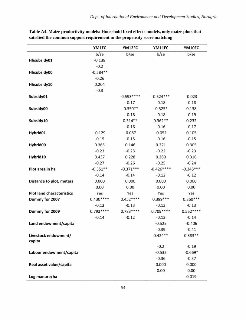
Dept. of International Environment and Development Studies, Noragric
54
Table A4. Maize productivity models: Household fixed effects models, only maize plots that satisfied the common support requirement in the propensity score matching
YM1FC YM12FC YM11FC YM10FC
b/se b/se b/se b/se Hhsubsidy01 -0.138 -0.2 Hhsubsidy00 -0.584** -0.26 Hhsubsidy10 0.204 -0.3 Subsidy01 -0.593**** -0.524*** -0.023 -0.17 -0.18 -0.18 Subsidy00 -0.350** -0.325* 0.138
-0.18 -0.18 -0.19 Subsidy10 0.314** 0.362** 0.232 -0.16 -0.16 -0.17 Hybrid01 -0.129 -0.087 -0.052 0.105 -0.15 -0.15 -0.16 -0.15 Hybrid00 0.365 0.146 0.221 0.305 -0.23 -0.23 -0.22 -0.23 Hybrid10 0.437 0.228 0.289 0.316 -0.27 -0.26 -0.25 -0.24 Plot area in ha -0.351** -0.371*** -0.426**** -0.345*** -0.14 -0.14 -0.12 -0.12 Distance to plot, meters 0.000 0.000 0.000 0.000 0.00 0.00 0.00 0.00 Plot land characteristics Yes Yes Yes Yes Dummy for 2007 0.430**** 0.452**** 0.389*** 0.360*** -0.13 -0.13 -0.13 -0.13 Dummy for 2009 0.793**** 0.783**** 0.709**** 0.552**** -0.14 -0.12 -0.13 -0.14 Land endowment/capita -0.525 -0.406 -0.39 -0.41 Livestock endowment/ capita
0.424** 0.383**
-0.2 -0.19 Labour endowment/capita -0.532 -0.669* -0.36 -0.37 Real asset value/capita 0.000 0.000 0.00 0.00 Log manure/ha 0.019
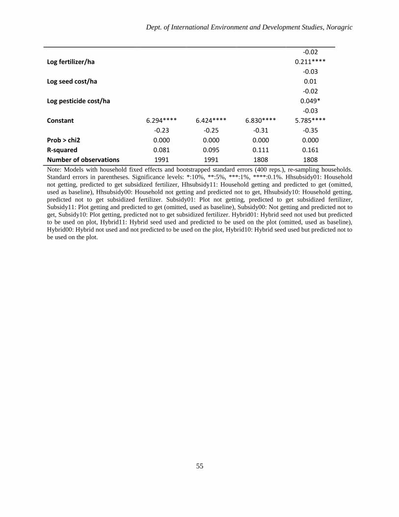
Dept. of International Environment and Development Studies, Noragric
55
-0.02 Log fertilizer/ha 0.211**** -0.03 Log seed cost/ha 0.01 -0.02 Log pesticide cost/ha 0.049* -0.03 Constant 6.294**** 6.424**** 6.830**** 5.785**** -0.23 -0.25 -0.31 -0.35 Prob > chi2 0.000 0.000 0.000 0.000 R-squared 0.081 0.095 0.111 0.161 Number of observations 1991 1991 1808 1808 Note: Models with household fixed effects and bootstrapped standard errors (400 reps.), re-sampling households. Standard errors in parentheses. Significance levels: *:10%, **:5%, ***:1%, ****:0.1%. Hhsubsidy01: Household not getting, predicted to get subsidized fertilizer, Hhsubsidy11: Household getting and predicted to get (omitted, used as baseline), Hhsubsidy00: Household not getting and predicted not to get, Hhsubsidy10: Household getting, predicted not to get subsidized fertilizer. Subsidy01: Plot not getting, predicted to get subsidized fertilizer, Subsidy11: Plot getting and predicted to get (omitted, used as baseline), Subsidy00: Not getting and predicted not to get, Subsidy10: Plot getting, predicted not to get subsidized fertilizer. Hybrid01: Hybrid seed not used but predicted to be used on plot, Hybrid11: Hybrid seed used and predicted to be used on the plot (omitted, used as baseline), Hybrid00: Hybrid not used and not predicted to be used on the plot, Hybrid10: Hybrid seed used but predicted not to be used on the plot.