Nonnegative Matrix Completion for Life-cycle

Assessment and Input-ouput Analysis

Fangfang Xu1, Chen Lin∗,2, Guoping He3, Zaiwen Wen4

Abstract

Life-cycle assessment (LCA) and input-output analysis (IOA) are two

data-intensive approaches whose reliability and applicability are dependent

on the quality of the data. The difficulty is that not all data is available

due to technical or cost reasons. However, the processes producing similar

commodities have similar data structures in LCA, while the sectors of the

historical surveyed years in IOA have similar input structures as the sectors

of the objective year. These features imply that the data usually has low-rank

or approximately low-rank structures which enables us to apply the emerging

techniques of low-rank matrix completion to recover the missing data. Since

the data should be nonnegative in LCA and IOA if we ignore the minor by-

product issue, we propose two models for nonnegative matrix completion to

recover the missing information of LCA and IOA. The alternating direction

method of multipliers is then applied to solve them. The applicability and

∗Corresponding author. Tel.:+86 13589112903; fax: +86 0531 88364981.Email address: c lin@sdu.edu.cn ( Chen Lin )

1Department of Mathematics, Shanghai Jiao Tong University, Shanghai 200240, China2The Center for Economic Research, Shandong University, Jinan 250100, China3College of Information Science and Engineering, Shandong University of Science and

Technology, Qingdao 266510, China4Beijing International Center for Mathematical Research, Peking University, Beijing

100871, China

Preprint submitted to CER working papers January 2, 2014

efficiency of our methods are demonstrated in an application to the widely

used database “Ecoinvent” for the life-cycle assessment. Recovering results

show that our approaches are helpful.

Key words: Missing data recovery, Nonnegative matrix completion,

Life-cycle assessment, Input-output analysis, Alternating direction method

of multipliers

1. Introduction

Matrix completion (MC) is the process of recovering the unknown or

missing elements of a matrix. Under some reasonable assumptions, an in-

complete but low-rank matrix can be reconstructed exactly (Candes and

Recht, 2009; Recht et al., 2010). The matrix completion problem is widely

applicable in many fields, such as machine learning(Abernethy et al., 2006),

control(Mesbahi and Papavassilopoulos, 1997), image and video process-

ing(Osher et al., 2005; Ji et al., 2010; Candes et al., 2011), where matrices

with low-rank structures are used in the model construction. Another poten-

tially applicable field is the life-cycle assessment (LCA). LCA is a method-

ology to assess the impacts associated with all the stages of a product’s life

from-cradle-to-grave, which is sensitive to the data quality. A technology

matrix consisting of production/consumption processes can be used to ob-

tain the result of life-cycle inventory (LCI) (Heijungs and Suh, 2002). The

technology matrix for LCI can suffer from the missing data problem for both

technical and cost reasons. For example, some types of inputs and outputs

are difficult to be attributed to a co-product from the multi-output process.

The reliability and thus the applicability of the results of an LCI is depen-

2

dent on the quality of the original data providing the background for the

assessment (Weidema and Wesnæs, 1996). The technology matrix of LCI

is usually low-rank due to the existence of enormous similar processes. For

example, the processes producing similar commodities and the analogous pro-

cesses in different countries have similar data structures (Huele and van den

Berg, 1998). Thus, the matrix completion method can be used to recover the

missing data.

IOA is another field of potential application of matrix completion, which

has similar data structure with LCA (Heijungs and Suh, 2002; Suh, 2004).

In the countries who have the input-output (IO) tables, the statistic depart-

ments publish the IO tables only for certain years by survey (Miller and

Blair, 2009). For example, China, Japan, and US publish the survey tables

for every 5 years (National Bureau of Statistics of China, 2012; Minstry of In-

ternal Affairs and Communication of Japan, 2012; U.S. Bureau of Economic

Analysis, 2012). However, when the economists want to do the economic

analysis for the other non-surveyed years, data for the objective year needs

to be estimated. Only a limited statistical information can be used to esti-

mate the input-output table of the non-surveyed years, while the part of the

table without statistical information are missing. The statistic information

and historical IO tables, whose sectors have high correlation with the objec-

tive year’s sectors, can be used to estimate the IO tables of the objective

year by using the matrix completion method. It is because the correlativity

makes the matrix in question be low-rank or approximately low-rank. In

the context of IO, our method can be an alternative estimation method of

non-surveyed IO tables other than RAS.

3

Additionally, Suh (2004) proposed the hybrid LCA method by combin-

ing the general IO data with the process-based data to extend the system

boundary of LCA. The correlation between IO sectors and processes makes

the technology matrix used in the hybrid method be low-rank or approxi-

mately low-rank. This implies the possibility of applying the matrix com-

pletion method to recover the missing data and improve the data quality for

hybrid LCA studies, such as Nakamura and Kondo (2006) and Lin (2011).

It is important to note that the above mentioned technology matrices in

LCA and IO are nonnegative if we ignore the minor by-product issue. This

motivates the development of the nonnegative matrix completion.

Recently, there have been extensive researches on low-rank matrix com-

pletion (LRMC), which aims to find a matrix of minimum rank under cer-

tain linear constraints. However, the model is NP-hard (non-deterministic

polynomial-time hard, Natarajan (1995)) due to the combinatorial nature of

the rank function. Candes and Recht (2009) and Recht et al. (2010) show

that rank function can be replaced with nuclear norm under some reason-

able conditions in order to get a convex problem. As we all known, convex

problems can be much easily solved and their local optimal solutions are

global. More details about LRMC can be found in (Fazel, 2002; Ma et al.,

2009; Candes and Tao, 2010; Cai et al., 2010; Wen et al., 2012; Xu et al.,

2012) and references therein. From the numerical experiments of the above

literatures, recovery results are very good even when matrices are only ap-

proximately low-rank. In practice, certain constraint is usually imposed on

the recovered matrix, such as positive semi-definite (Chen et al. (2012)) or

nonnegative (Xu et al. (2012)) constraints. Therefore, efficient algorithms

4

are needed to conduct these special matrix completion tasks.

In this paper, we aim to develop efficient algorithms of nonnegative ma-

trix completion to recover the missing data in LCA and IOA. Suppose that

technology matrix of LCA and IOA is nonnegative and low-rank or approx-

imately low-rank. Therefore, technology matrix can be completed using the

solvers of nonnegative matrix completion when some elements are missing.

We propose two models based on whether the known elements of the matrix

are contaminated by noise or not. The structure of the two models suggests

that the alternating direction method of multipliers (ADMM) is suitable to

solve them, that is, one can update each of the variables efficiently while

fixing the others. Two ADMM-based algorithms are proposed to conduct

nonnegative matrix completion. As an application, we apply the proposed

algorithms to recover the potentially missing data in Ecoinvent database—a

widely used database of LCA. Recovering results show that our new algo-

rithms can be helpful.

The rest of this paper is organized as follows. The applicability of matrix

completion in LCA and IOA is discussed in section 2. We present our nonneg-

ative matrix completion models and algorithms in section 3. The numerical

experiments on the Ecoinvent database are present in section 4.

The following notations will be used throughout this paper. Upper (lower)

face letters are used for matrices (column vectors). All vectors are col-

umn vectors, the superscript (·)T denotes matrix and vector transposition.

Diag(x) denotes a diagonal matrix with x on its main diagonal. 0 is a matrix

of all zeros of proper dimension, In stands for the n×n identity matrix. The

trace of A ∈ Rm×n, i.e., the sum of the diagonal elements of A, is denoted by

5

tr(A). The Frobenius norm of A ∈ Rm×n is defined as ‖A‖F =√∑

i,j |Ai,j|2.

The Euclidean inner product between two vectors x ∈ Rn and y ∈ Rn is de-

fined as 〈x, y〉 =∑n

i=1 xiyi. The Euclidean inner product between two matri-

ces A ∈ Rm×n and Z ∈ Rm×n is defined as 〈A,Z〉 =∑

i,j(Ai,jZi,j) = tr(A>Z).

The inequality A ≥ 0 is element-wise, which means Aij ≥ 0 for all entries

(i, j). Likewise, the equality A = Z means Aij = Zij for all entries (i, j).

2. Applicability of MC in LCA and IOA

2.1. LCA and hybrid LCA

LCA is a technique to assess the environmental impacts of a product

throughout its life cycle. According to Heijungs and Suh (2002) and Suh

(2004), the LCA can be calculated by using the calculation structure that is

the same with the environmentally extended input-output model (Leontief,

1970; Duchin, 1990),

q = B(I − A)−1y, (1)

where y refers to the bundle of products of interest, whose ith element refers

to the amount of product produced by process i. The matrix A refers to

the technology matrix whose element Ai,j shows the amount of input from

process i in producing a unit of output by process j. Note that if we rule

out the minor by-product issues, the matrix A is nonnegative. The matrix

I is the identity, B is the environmental intervention, in which element Bi,j

denotes the amount of environmental intervention i generated in producing

a unit of output by process j, and q refers to the total environmental impact.

The A matrix usually has low rank or approximately low rank due to

the existence of enormous similar processes. For example, in Ecoinvent V2.1

6

(Frischknecht et al., 2005), among all 3963 unit-processes there are 228 pro-

cesses of electricity generation, 55 processes of road vehicle operations, etc.

If there are missing data in the original technology matrix A0 provided by

a database—namely a part of elements of the matrix A0 is unknown while

the other part is known, MC can be used to recover the missing data. In the

application part of the paper, our approach will be applied to the Ecoinvent’s

technology matrix.

2.2. IOA

In IOA, the intermediate input coefficient matrix, which is similar to the

technology matrix in LCA, is used in the Leontief quantity model and the

price model (Leontief, 1936, 1985). As mentioned previously, in the context

of IOA, we are interested in estimating the intermediate input matrix of

the non-surveyed years. First, by using the limited statistic information,

we can make an uncompleted intermediate input coefficient matrix of the

objective non-surveyed year, At, whose ijth element shows the amount of

input from sector i in producing a unit of output by sector j. A part of

A0t ’s elements is known by using the statistic information, while the other

part is unknown and needs to be recovered. Accomplishing with the known

intermediate coefficient input matrices of the surveyed years, we can build

an original matrix for MC,

A0 =(A0t−n ... A0

t−1 A0t A0

t+1 ... A0t+n

), (2)

where A0i , i 6= t, refers to the known intermediate input coefficient matrices

of the surveyed year i. We use the original A0 to estimate the completed

7

A. The A matrix is nonnegative if we do not consider the minor by-product

issues. Because the sectors of the surveyed years are correlated with the

sectors of the objective year, A should satisfy the low-rank or approximately

low-rank assumption and the MC is applicable. Based on the original A0

matrix, our MC approach gives the completed

A =(At−n ... At−1 At At+1 ... At+n

), (3)

where At is the estimated intermediate input coefficient matrix of the objec-

tive year.

3. Nonnegative Matrix Completion

We now propose two models of nonnegative matrix completion to recover

the missing information of the nonnegative matrix A mentioned in Section 2.1

and 2.2. Both models can be solved by the alternating direction method of

multipliers. For more details about ADMM, please refer to He et al. (2010);

Wen et al. (2010); Boyd et al. (2011).

3.1. Models for Nonnegative Matrix Completion

The matrix completion problem with nonnegative constraints is in the

following form:

min rank(A)

s.t. Aij = A0ij, for all (i, j) ∈ Ω,

A ≥ 0,

(4)

where A ∈ Rm×n is the decision variable, and A0i,j ∈ R are given known

elements of matrix A for (i, j) ∈ Ω ⊂ (i, j) : 1 ≤ i ≤ m, 1 ≤ j ≤ n. Let

8

PΩ be the projection onto the subspace of matrices with non-zeros elements

restricted to the index subset Ω, i.e.,

PΩ(A)ij =

Aij, if (i, j) ∈ Ω,

0, otherwise.

It follows from the definition of PΩ that the equality constraints in Model 4

can be reformulated as PΩ(A) = PΩ(A0). Due to the combinational property

of the objective function rank(·), Model 4 is NP-hard in general. Inspired by

the success of matrix completion under nuclear norm in Candes and Recht

(2009); Recht et al. (2010); and Candes and Tao (2010), we use the nuclear

norm as an approximation to rank(A) to estimate the optimal solution A∗

of Model 4 from the nuclear norm minimization problem with linear and

nonnegative constraints:

min ‖A‖∗

s.t. PΩ(A) = PΩ(A0),

A ≥ 0,

(5)

where the nuclear norm ‖A‖∗ of A is defined as the summation of the singular

values of A, i.e.,

‖A‖∗ =

min(m,n)∑i=1

σi(A),

where σi(A) is the ith largest singular value of A.

If the known elements of the matrix A are exact, that is to say PΩ(A0)

is reliable, Model 5 is suitable to treat this noise free case. On the contrary,

9

the constraint PΩ(A) = PΩ(A0) must be relaxed if PΩ(A0) is contaminated

by noise, resulting in either problem:

minA∈Rm×n

‖A‖∗, s.t. ||PΩ(A)− PΩ(A0)|| 6 δ, A ≥ 0, (6)

or the nuclear norm regularized linear least squares model with nonnegative

constraints:

minA∈Rm×n

µ‖A‖∗ +1

2‖PΩ(A)− PΩ(A0)‖2

2, s.t. A ≥ 0. (7)

Here, δ and µ are given parameters, whose values should be set according to

the noise level. Models 6 and 7 are equivalent when the parameters µ and

δ are set properly. In this paper, we choose Model 7 to treat the condition

in which the known elements of the matrix of interest are contaminated by

noise, but our approach can be extended to Model 6 without any difficulty.

Model 7 is especially useful in the context of LCA and IOA. The reason is

that the known elements of the technology matrices are usually gotten from

large surveys and contaminated by sampling error inevitably. For the sources

of uncertainty and variability, we refer the reader to Table 1 in Lloyd and

Ries (2007).

3.2. An Alternating Direction Method of Multipliers for Model 5

In this subsection, we present an ADMM-based algorithm for Model 5.

To facilitate an efficient use of ADMM, we introduce a new matrix variable

10

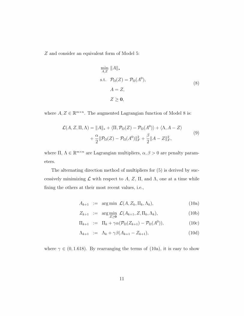
Z and consider an equivalent form of Model 5:

minA,Z‖A‖∗

s.t. PΩ(Z) = PΩ(A0),

A = Z,

Z ≥ 0,

(8)

where A,Z ∈ Rm×n. The augmented Lagrangian function of Model 8 is:

L(A,Z,Π,Λ) = ‖A‖∗ + 〈Π,PΩ(Z)− PΩ(A0)〉+ 〈Λ, A− Z〉

+α

2‖PΩ(Z)− PΩ(A0)‖2

F +β

2‖A− Z‖2

F ,(9)

where Π, Λ ∈ Rm×n are Lagrangian multipliers, α, β > 0 are penalty param-

eters.

The alternating direction method of multipliers for (5) is derived by suc-

cessively minimizing L with respect to A, Z, Π, and Λ, one at a time while

fixing the others at their most recent values, i.e.,

Ak+1 := arg min L(A,Zk,Πk,Λk), (10a)

Zk+1 := arg minZ≥0

L(Ak+1, Z,Πk,Λk), (10b)

Πk+1 := Πk + γα(PΩ(Zk+1)− PΩ(A0)), (10c)

Λk+1 := Λk + γβ(Ak+1 − Zk+1), (10d)

where γ ∈ (0, 1.618). By rearranging the terms of (10a), it is easy to show

11

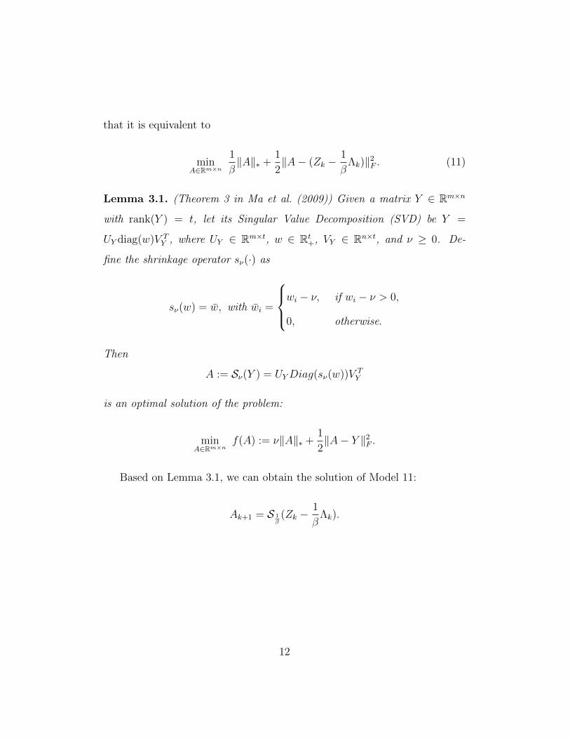
that it is equivalent to

minA∈Rm×n

1

β‖A‖∗ +

1

2‖A− (Zk −

1

βΛk)‖2

F . (11)

Lemma 3.1. (Theorem 3 in Ma et al. (2009)) Given a matrix Y ∈ Rm×n

with rank(Y ) = t, let its Singular Value Decomposition (SVD) be Y =

UY diag(w)V TY , where UY ∈ Rm×t, w ∈ Rt

+, VY ∈ Rn×t, and ν ≥ 0. De-

fine the shrinkage operator sν(·) as

sν(w) = w, with wi =

wi − ν, if wi − ν > 0,

0, otherwise.

Then

A := Sν(Y ) = UYDiag(sν(w))V TY

is an optimal solution of the problem:

minA∈Rm×n

f(A) := ν‖A‖∗ +1

2‖A− Y ‖2

F .

Based on Lemma 3.1, we can obtain the solution of Model 11:

Ak+1 = S 1β(Zk −

1

βΛk).

12

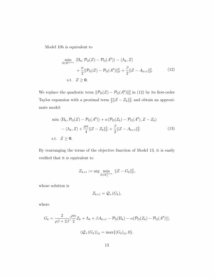
Model 10b is equivalent to

minZ∈Rm×n

〈Πk,PΩ(Z)− PΩ(A0)〉 − 〈Λk, Z〉

+α

2‖PΩ(Z)− PΩ(A0)‖2

F +β

2‖Z − Ak+1‖2

F

s.t. Z ≥ 0.

(12)

We replace the quadratic term ‖PΩ(Z)− PΩ(A0)‖22 in (12) by its first-order

Taylor expansion with a proximal term ρ2‖Z − Zk‖2

F and obtain an approxi-

mate model:

min 〈Πk,PΩ(Z)− PΩ(A0)〉+ α〈PΩ(Zk)− PΩ(A0), Z − Zk〉

− 〈Λk, Z〉+ρα

4‖Z − Zk‖2

F +β

2‖Z − Ak+1‖2

F

s.t. Z ≥ 0.

(13)

By rearranging the terms of the objective function of Model 13, it is easily

verified that it is equivalent to

Zk+1 := arg minZ∈Rm×n

+

‖Z −Gk‖2F ,

whose solution is

Zk+1 = Q+(Gk),

where

Gk =2

ρβ + 2β[ρα

2Zk + Λk + βAk+1 − PΩ(Πk)− α(PΩ(Zk)− PΩ(A0))],

(Q+(Gk))ij = max(Gk)ij, 0.

13

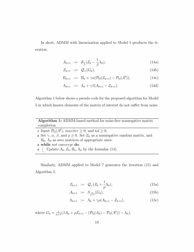
In short, ADMM with linearization applied to Model 5 produces the it-

eration:

Ak+1 := S 1β(Zk −

1

βΛk), (14a)

Zk+1 := Q+(Gk), (14b)

Πk+1 := Πk + γα(PΩ(Zk+1)− PΩ(A0)), (14c)

Λk+1 := Λk + γβ(Ak+1 − Zk+1). (14d)

Algorithm 1 below shows a pseudo code for the proposed algorithm for Model

5 in which known elements of the matrix of interest do not suffer from noise.

Algorithm 1: ADMM-based method for noise-free nonnegative matrixcompletion

1 Input PΩ(A0), maxiter ≥ 0, and tol ≥ 0.2 Set γ, α, β, and ρ ≥ 0. Set Z0 as a nonnegative random matrix, and

Π0, Λ0 as zero matrices of appropriate sizes.3 while not converge do4 Update Ak, Zk,Πk,Λk by the formulas (14).

Similarly, ADMM applied to Model 7 generates the iteration (15) and

Algorithm 2.

Zk+1 := Q+(Zk +1

ρΛk), (15a)

Ak+1 := S µρ+β

(Gk), (15b)

Λk+1 := Λk + γρ(Ak+1 − Zk+1), (15c)

where Gk = 1ρ+β

(βAk + ρZk+1 − (PΩ(Ak)− PΩ(A0))− Λk).

14

Algorithm 2: ADMM-based method for nonnegative matrix comple-tion with noise1 Input PΩ(A0), maxiter ≥ 0, and tol ≥ 0.2 Set ρ, µ, γ, and β ≥ 0. Set Z0 as a random matrix, and Λ0 as zero

matrices of appropriate sizes.3 while not converge do4 Update Zk, Ak,Λk by the formulas (15).

The convergence of the above two schemes is ensured by the theory in

(Hong and Luo, 2012).

4. Application

In this section, Algorithms 1 and 2 are applied to the recovery of the

potentially missing data in Ecoinvent database V2.1 (Frischknecht et al.,

2005). There are 3964 unit-processes to build the original technology matrix

A0 for recovery, which is a 3964 × 3964 square matrix. Its element A0i,j

shows the amount of input from process i in producing a unit of output

by process j. We assume that there are missing data in A0 matrix given

by Ecoinvent database and our goal is to complete the matrix by using our

method. The non-zero elements in A0 are considered to be known elements.

However, we can not argue that all the zero elements in A0 are potentially

unknown elements. It is because not all the 3964 × 3964 elements in the

matrix should have non-zero values, since technically there may not be any

input from a certain process to another certain process. In order to find the

should-be-zero elements, we relate every Ecoinvent process to an sector of

the US input-output (IO) table. Multiple Ecoinvent processes can belong to

an IO sector because the IO sector is more general than Ecoinvent processes.

15

To be exact, let the IO sector related to Ecoinvent process i be sector io.

Let Θ be the set of the should-be-zero elements. Then we define A0i,j ∈ Θ if

Biojo = 0, where Bio,jo refers to the element of the intermediate input matrix

B of US IO table. This means that if there exists no input from IO sector

io to IO sector jo, there should be no input from the Ecoinvent processes in

IO sector io to the Ecoinvent processes belonging to IO sector jo. In this

case, the size of Θ is 3,197,414. Let the set of non-zero element in A0 be Γ

(31,950 elements). Consequently, the set of known elements can be given by

Ω = Γ∪Θ, which has 3,229,364 elements. The information from Ω is used to

recover the potentially missing data in A0. We rule out the minor by-product

issues, which implies that the A0 matrix is nonnegative. With regard to the

environmental pressure data (or output flow data) of Ecoinvent, although

its recovery is not included in the current application, our approach is also

applicable because of the similarity of data structure.

All algorithms are implemented in MATLAB and all experiments were

performed on a Dell Precision T5500 workstation with Intel(R) Xenon(R)

E5620 CPU at 2.40GHz (×4) and 12GB of memory running Ubuntu 12.04

and MATLAB 2011b.

4.1. Experiments on noise-free Data

As mentioned previously, 3,229,364 elements (about 20% of elements in

A0) are known, the rest (12,483,932 elements) are unknown or missing. In

order to check the accuracy of our algorithms, we select a subset of a%

uniformly at random from the known elements set Ω and denote it by Ω1.

The residual (100−a)% of the known elements is denoted by Ω2. We use Ω1 to

conduct nonnegative matrix completion, then use Ω2 to compute precision of

16

our algorithms. In summary, we divide the known elements set Ω to Ω1 (used

for nonnegative matrix completion) and Ω2 (used for computing precision).

For Algorithm 1, we set γ = 1.618, the value of α = 0.1, β = 0.1, and

ρ = 0.01. The algorithm is stopped if a maximal number of 103 iterations is

reached or if the following conditions are satisfied:

‖Ak+1 − Ak‖Fmax(1, ‖Ak‖F )

≤ tol, (16a)

‖Ak+1 − Zk+1‖F ≤ tol, (16b)

‖PΩ(Zk+1)− PΩ(A0)‖2 ≤ tol, (16c)

where tol is set to be 10−4. Finally, Algorithm 1 outputs the completed A

as the estimation of the full technology matrix based on A0. The average

relative errors of the elements belonging to Ω1 and Ω2 are denoted by err1

and err2, respectively:

err1 =

√∑(i,j)∈Ω1

(Aij−A0

ij

max(1,A0ij)

)2

|Ω1|,

err2 =

√∑(i,j)∈Ω2

(Aij−A0

ij

max(1,A0ij)

)2

|Ω2|.

Both err1 and err2 are computed when a is equal to 80, 85, 90, 95, or

100. The results are shown in Table 1, where p is the cardinality of set Ω1

(number of the elements in Ω1). p is also the number of the known elements

used to conduct nonnegative matrix completion.

From Table 1, we can observe that when a increase from 80 to 100, err1

17

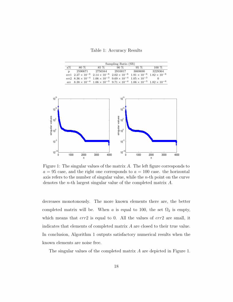
Table 1: Accuracy Results

Sampling Ratio (SR)a% 80 % 85 % 90 % 95 % 100 %p 2590671 2750344 2910017 3069690 3229364

err1 2.27× 10−6 2.14× 10−6 2.02× 10−6 1.91× 10−6 1.82× 10−6

err2 8.36× 10−4 1.06× 10−3 9.69× 10−4 1.05× 10−3 0err 8.38× 10−4 1.06× 10−3 9.71× 10−4 1.06× 10−3 1.82× 10−6

0 1000 2000 3000 400010

−10

10−5

100

105

1010

1015

sin

gu

lar

va

lues

n0 1000 2000 3000 4000

10−10

10−5

100

105

1010

1015

sin

gu

lar

va

lues

n

Figure 1: The singular values of the matrix A. The left figure corresponds toa = 95 case, and the right one corresponds to a = 100 case. the horizontalaxis refers to the number of singular value, while the n-th point on the curvedenotes the n-th largest singular value of the completed matrix A.

decreases monotonously. The more known elements there are, the better

completed matrix will be. When a is equal to 100, the set Ω2 is empty,

which means that err2 is equal to 0. All the values of err2 are small, it

indicates that elements of completed matrix A are closed to their true value.

In conclusion, Algorithm 1 outputs satisfactory numerical results when the

known elements are noise free.

The singular values of the completed matrix A are depicted in Figure 1.

18

We observe that the singular values decrease quickly and there are only a

few dominant singular values. Specifically, the 500th largest singular value

is already close to 1. Therefore, A is low-rank or approximately low-rank.

4.2. Experiments on data with Noise

We now apply Algorithm 1 and 2 to the recovery of Ecoinvent technology

matrix when the known elements are contaminated by noise.

The parameter µ in Model 7 is usually set to be a medium value between 0

to 10 in general. We can use continuation technique to speed the convergence

of Algorithm 2. We solve a sequence of Model 7 defined by a decreasing

sequence µ0, µ1, . . . , µl = µ with a finite positive integer l. We set µ =

10−4µ0 with the initial µ0 = 100, and update µk = max0.7µk−1, µ at

iteration k. All the other parameters are set to be the same as Section 5.1.

Suppose that PΩ(A0) is contaminated and ε is the error ratio. We select

M between PΩ(A0) − εPΩ(A0) and PΩ(A0) + εPΩ(A0) at random, that is

to say, PΩ(A0) − εPΩ(A0) ≤ M ≤ PΩ(A0) + εPΩ(A0). Then M is used to

conduct nonnegative matrix completion using Algorithm 1 and 2. The results

are shown in Table 2 corresponding to different ε. In this subsection, a is set

to be 95.

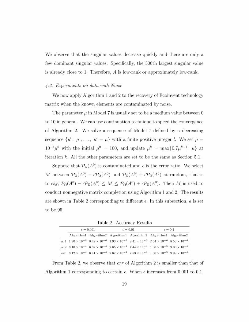
Table 2: Accuracy Results

ε = 0.001 ε = 0.01 ε = 0.1

Algorithm1 Algorithm2 Algorithm1 Algorithm2 Algorithm1 Algorithm2

err1 1.90× 10−6 8.42× 10−6 1.93× 10−6 8.41× 10−6 2.64× 10−6 8.53× 10−6

err2 8.10× 10−4 6.32× 10−4 9.65× 10−4 7.44× 10−4 1.30× 10−3 9.90× 10−4

err 8.12× 10−4 6.41× 10−4 9.67× 10−4 7.53× 10−4 1.30× 10−3 9.99× 10−4

From Table 2, we observe that err of Algorithm 2 is smaller than that of

Algorithm 1 corresponding to certain ε. When ε increases from 0.001 to 0.1,

19

err of Algorithm 2 increases slower than that of Algorithm 1. Therefore, the

recovery results of Algorithm 2 are better than those of Algorithm 1 when

the known elements are contaminated. It also means that Algorithm 2 is

more robust.

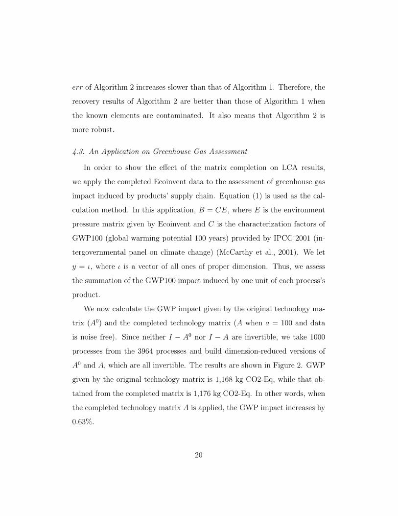
4.3. An Application on Greenhouse Gas Assessment

In order to show the effect of the matrix completion on LCA results,

we apply the completed Ecoinvent data to the assessment of greenhouse gas

impact induced by products’ supply chain. Equation (1) is used as the cal-

culation method. In this application, B = CE, where E is the environment

pressure matrix given by Ecoinvent and C is the characterization factors of

GWP100 (global warming potential 100 years) provided by IPCC 2001 (in-

tergovernmental panel on climate change) (McCarthy et al., 2001). We let

y = ι, where ι is a vector of all ones of proper dimension. Thus, we assess

the summation of the GWP100 impact induced by one unit of each process’s

product.

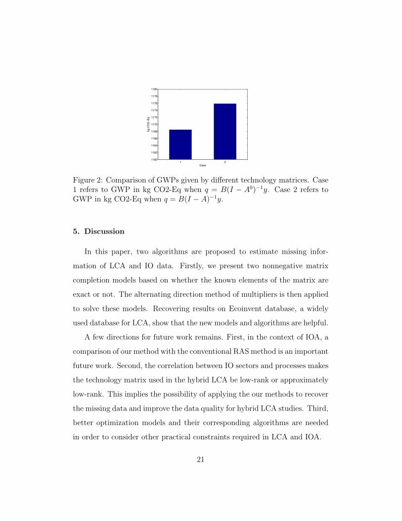
We now calculate the GWP impact given by the original technology ma-

trix (A0) and the completed technology matrix (A when a = 100 and data

is noise free). Since neither I − A0 nor I − A are invertible, we take 1000

processes from the 3964 processes and build dimension-reduced versions of

A0 and A, which are all invertible. The results are shown in Figure 2. GWP

given by the original technology matrix is 1,168 kg CO2-Eq, while that ob-

tained from the completed matrix is 1,176 kg CO2-Eq. In other words, when

the completed technology matrix A is applied, the GWP impact increases by

0.63%.

20

1 21160

1162

1164

1166

1168

1170

1172

1174

1176

1178

1180

kg C

O2−

Eq

Case

Figure 2: Comparison of GWPs given by different technology matrices. Case1 refers to GWP in kg CO2-Eq when q = B(I − A0)−1y. Case 2 refers toGWP in kg CO2-Eq when q = B(I − A)−1y.

5. Discussion

In this paper, two algorithms are proposed to estimate missing infor-

mation of LCA and IO data. Firstly, we present two nonnegative matrix

completion models based on whether the known elements of the matrix are

exact or not. The alternating direction method of multipliers is then applied

to solve these models. Recovering results on Ecoinvent database, a widely

used database for LCA, show that the new models and algorithms are helpful.

A few directions for future work remains. First, in the context of IOA, a

comparison of our method with the conventional RAS method is an important

future work. Second, the correlation between IO sectors and processes makes

the technology matrix used in the hybrid LCA be low-rank or approximately

low-rank. This implies the possibility of applying the our methods to recover

the missing data and improve the data quality for hybrid LCA studies. Third,

better optimization models and their corresponding algorithms are needed

in order to consider other practical constraints required in LCA and IOA.

21

6. Acknowledgements

The work of F. Xu and G. He was supported in part by NSFC (Grant No.

10971122), Scientific and Technological Projects (2009GG10001012) of Shan-

dong Province and Excellent Young Scientist Foundation (2010BSE06047,

BS2012SF025) of Shandong Province. The work of C. Lin was supported

in part by Shandong Province Natural Science Foundation (ZR2012GQ004)

and Independent Innovation Foundation (IFW12098) of Shandong Univer-

sity. The work of Z. Wen was supported in part by NSFC grant 11101274

and Research Fund (20110073120069) for the Doctoral Program of Higher

Education of China.

References

Abernethy, J., Bach, F., Evgeniou, T., et al., 2006. Low-rank matrix factor-

ization with attributes. Tech. rep., arXiv preprint cs/0611124.

Boyd, S., Parikh, N., Chu, E., et al., 2011. Distributed optimization and sta-

tistical learning via the alternating direction method of multipliers. Foun-

dations and Trends in Machine Learning 3, 1–122.

Cai, J.-F., Candes, E. J., Shen, Z., 2010. A singular value thresholding algo-

rithm for matrix completion. SIAM J. Op 20, 1956–1982.

Candes, E. J., Eldar, Y., Strohmer, T., Voroninski, V., 2011. Phase retrieval

via matrix completion. Tech. rep., Stanford University.

Candes, E. J., Recht, B., May 2009. Exact matrix completion via convex

optimization. Foundations of Computational Mathematics.

22

Candes, E. J., Tao, T., 2010. The power of convex relaxation: near-optimal

matrix completion. IEEE Trans. Inform. Theory 56 (5), 2053–2080.

Chen, C., He, B., Yuan, X., 2012. Matrix completion via an alternating

direction method. IMA Journal of Numerical Analysis 32, 227–245.

Duchin, F., 1990. The conversion of biological materials and wastes to useful

products. Structural Change and Economic Dynamics 1 (2), 243–261.

Fazel, M., 2002. Matrix rank minimization with application. Ph.D. thesis,

Stanford University.

Frischknecht, R., Jungbluth, N., Althaus, H., Doka, G., Dones, R., Heck,

T., Hellweg, S., Hischier, R., Nemecek, T., Rebitzer, G., et al., 2005. The

ecoinvent database: Overview and methodological framework (7 pp). The

International Journal of Life Cycle Assessment 10 (1), 3–9.

He, B., Tao, M., Yuan, X., 2010. Alternating direction method with gaussian

back substitution for separable convex programming. Tech. rep., Nanjing

University.

Heijungs, R., Suh, S., 2002. The computational structure of life cycle assess-

ment. Vol. 11. Kluwer Academic Publishers.

Hong, M., Luo, Z.-Q., Aug. 2012. On the Linear Convergence of the Alter-

nating Direction Method of Multipliers. ArXiv e-prints.

Huele, R., van den Berg, N., 1998. Spy plots. The International Journal of

Life Cycle Assessment 3 (2), 114–118.

23

Ji, H., Liu, C., Shen, Z., et al., 2010. Robust video denoising using low

rank matrix completion. In: Computer Vision and Pattern Recognition

(CVPR), 2010 IEEE Conference on. IEEE. pp. 1791–1798.

Leontief, W., 1936. Quantitative input and output relations in the economic

systems of the united states. The review of Economics and Statistics 18 (3),

105–125.

Leontief, W., 1970. Environmental repercussions and the economic structure:

An input–output approach. Review of Economics and Statistics 52 (3),

262–271.

Leontief, W., 1985. Technological change, prices, wages, and rates of return

on capital in the u.s. economy. In: Leontief, W. (Ed.), input–output Eco-

nomics. Oxford: Oxford University Press, pp. 392–417.

Lin, C., 2011. Identifying lowest-emission choices and environmental pareto

frontiers for wastewater treatment input-output model based linear pro-

gramming. Journal of Industrial Ecology.

Lloyd, S. M., Ries, R., 2007. Characterizing, propagating, and analyzing

uncertainty in life-cycle assessment: A survey of quantitative approaches.

Journal of Industrial Ecology 11 (1), 161–179.

Ma, S., Goldfarb, D., Chen, L., 2009. Fixed point and bregman iterative

methods for matrix rank minimization. Mathematical Programming, 1–

33.

McCarthy, J. J., Canziani, O. F., Leary, N. A., Dokken, D. J., White, K. S.,

24

2001. Climate change 2001: impacts, adaptation, and vulnerability: con-

tribution of Working Group II to the third assessment report of the Inter-

governmental Panel on Climate Change. Cambridge University Press.

Mesbahi, M., Papavassilopoulos, G. P., 1997. On the rank minimization prob-

lem over a positive semidefinite linear matrix inequality. IEEE Transac-

tions on Automatic Control 42, 239–243.

Miller, R., Blair, P., 2009. Input-output analysis: foundations and extensions.

Cambridge University Press.

Minstry of Internal Affairs and Communication of Japan, 2012. Input-output

table of Japan. Accessed December 2012.

URL http://www.stat.go.jp/data/io/index.htm

Nakamura, S., Kondo, Y., 2006. A waste input–output life-cycle cost anal-

ysis of the recycling of end-of-life electrical home appliances. Ecological

Economics 57 (3), 494–506.

Natarajan, B. K., 1995. Sparse approximation solutions to linear systems.

SIAM J. Comput. 24 (2), 227–234.

National Bureau of Statistics of China, 2012. Input-output table of china.

Accessed December 2012.

URL http://www.stats.gov.cn/tjsj/qtsj/trccb/

Osher, S., Burger, M., Goldfarb, D., et al., 2005. An iterative regulariza-

tion method for total variation-based image restoration. Multiscale Model.

Simul. 4, 460–489.

25

Recht, B., Fazel, M., Parrilo, P. A., 2010. Guaranteed minimum-rank so-

lutions of linear matrix equations via nuclear norm minimization. SIAM

Rev. 52 (3), 471–501.

Suh, S., 2004. Functions, commodities and environmental impacts in an

ecological–economic model. Ecological Economics 48 (4), 451–467.

U.S. Bureau of Economic Analysis, 2012. Benchmark input-output data. Ac-

cessed December 2012.

URL http://www.bea.gov/industry/io_benchmark.htm

Weidema, B., Wesnæs, M., 1996. Data quality management for life cycle

inventoriesan example of using data quality indicators. Journal of Cleaner

Production 4 (3), 167–174.

Wen, Z., Goldfarb, D., Yin, W., 2010. Alternating direction augmented la-

grangian methods for semidefinite programming. Mathematical Program-

ming Computation 2 (3-4), 203–230.

Wen, Z., Yin, W., Zhang, Y., 2012. Solving a low-rank factorization model

for matrix completion by a nonlinear successive over-relaxation algorithm.

Math. Prog. Comp. 4, 333–361.

Xu, Y., Yin, W., Wen, Z., Zhang, Y., 2012. An alternating direction algo-

rithm for matrix completion with nonnegative factors. Frontiers of Math-

ematics in China 7, 365–384.

26