Nonlinear Model-Based Control of Thin-Film Drying for ...web.mit.edu/braatzgroup/nonlinear_model_based_control_of_thin_film... · Nonlinear Model-Based Control of Thin-Film Drying

Nonlinear Model-Based Control of Thin-Film Drying for ContinuousPharmaceutical ManufacturingAli Mesbah, Ashlee N. Ford Versypt, Xiaoxiang Zhu, and Richard D. Braatz*

Department of Chemical Engineering, Massachusetts Institute of Technology, 77 Massachusetts Avenue, Cambridge, Massachusetts02139, United States

ABSTRACT: This paper considers the model-based control of composition and thickness for a thin-film drying process used inthe continuous manufacturing of pharmaceutical tablets. In this nonlinear distributed dynamical system, a drug formulationsolution is coated onto a moving surface and then dried to form thin films of approximately 250 μm in thickness. A dynamicoptimizer is designed that employs a first-principles process model to simulate the spatial distribution of solvent concentration inthe film and the thin film shrinkage during drying. A critical parameter to describe the highly nonlinear dynamics of the thin-filmdrying is the mutual polymer−solvent diffusion coefficient, which strongly depends on solvent concentration and filmtemperature. Two optimal control problems are studied for set point tracking of solvent concentration and minimization ofenergy consumption in the dryer while satisfying various operational and product quality constraints. An unscented Kalman filteris designed to facilitate the output feedback implementation of the dynamic optimizer and to estimate unmeasured thin-filmquality attributes such as the film thickness. The performance of the model-based controller is compared to that of a proportionalintegral controller in two simulation case studies. The nonlinear model-based control strategy has improved versatility and thepotential to reduce production of off spec material.

1. INTRODUCTIONContinuous manufacturing is receiving increasing attention inthe pharmaceutical industry to reduce time-to-market andproduction costs while enhancing product quality.1,2 Tradi-tionally, the batch mode of operation dominates thepharmaceutical industry. A shift from the batch mode ofoperation to the continuous mode, where raw materials areconverted to the drug products in an integrated facility, offersopportunities to improve the overall flexibility, reliability, andefficiency of the production process.3,4 In addition, continuousmanufacturing facilitates the use of increased process under-standing for online process control,5 which can lead toconsistently higher quality products as well as reduced wastegeneration and energy consumption.The majority of pharmaceutical products are manufactured as

solid tablets or capsules due to their low manufacturing cost,effective delivery of active pharmaceutical ingredients (APIs),designable disintegration profiles, and convenience of use.6,7

However, tablets and capsules are composed of powders, whichare difficult to handle and, more importantly, may lack APIuniformity.8 To address the manufacturing challenges of soliddosage forms, thin films that dissolve quickly have beendeveloped as an oral drug delivery system in recent years.9,10

Thin-film manufacturing is based on liquid solutions, whichalleviate the solids-handling problems. Thin-film dosage formsare especially advantageous when the API cannot be dispersedwell in a solid form or the solids handling reduces the APIyield,11 but the use of dissolving oral films is limited to APIswith fast metabolic uptake rates due to the rapid disintegrationof thin films. The storage and transportation of thin films is alsochallenging because of their fragility and friability.12

A process of manufacturing pharmaceutical tablets from thinfilms has been developed at the Novartis−MIT Center forContinuous Manufacturing.8 The continuous process for

making thin-film tablets consists of four steps: preparation ofthe formulation solution, casting the solution as a thin layer thatis dried to produce the thin film, folding of the dried thin film,and compaction of the folded thin film to form tablets. Thisprocess combines the merits of thin-film manufacturing interms of minimal solids handling and fast drying times with thewider applicability of tablets for effective drug delivery.This paper investigates advanced control of a continuous

thin-film dryer that comprises the second step of the thin-filmtablet manufacturing process. The film is coated onto a movingsurface and dried in the thin-film dryer to remove solvents inthe drug formulation solution. The mechanical characteristicsand adhesion properties of thin films used in subsequent filmfolding, compaction, and extrusion operations heavily rely onthe solvent composition in the film at the end of the dryingprocess.8 Controlling the solvent content and thickness of thethin film exiting the dryer is critical to the overall process ofthin-film tablet formation.In general, the control problem for film coating processes is

separated into two control objectives: maintenance of uniformthickness along the length of the film, known in the literature asthe machine-direction control problem, and maintenance ofuniform properties across the width of the film, known as thecross-directional control problem (see the work of VanAntwerp etal.13 and references therein). The control objective for the thin-film dryer studied in this paper is to regulate the film properties(composition and thickness) as the film moves through the

Special Issue: John Congalidis Memorial

Received: August 28, 2013Revised: December 18, 2013Accepted: December 18, 2013Published: December 18, 2013

Article

pubs.acs.org/IECR

© 2013 American Chemical Society 7447 dx.doi.org/10.1021/ie402837c | Ind. Eng. Chem. Res. 2014, 53, 7447−7460

pubs.acs.org/IECR

dryer. The system dynamics in this machine-directional controlproblem are characterized by highly nonlinear dynamics in thecomposition evolution in the film, a characteristic that is sharedby many other sheet and film processes.14−17 In addition, dueto their high costs, only a limited number of in situ sensors areusually used to measure the uniformity of film properties(especially film thickness) for online control applications.18,19

In this study, a nonlinear model-based controller isdeveloped for optimal operation of the thin-film dryer. Theuse of model predictive control has long been considered forthe control of sheet and film coating processes.20−29 Whatdistinguishes this work is the complex nonlinear distributeddynamics of composition evolution and the nonlinear filmshrinkage throughout the drying process that necessitate theuse of nonlinear state estimation and control techniques. Dueto the change in film properties as the thin film moves throughthe dryer, there is a one-to-one correspondence between thedrying time and the position of the film in the dryer. Thiscorrespondence implies that the control problem should beformulated with respect to a spatial domain and, therefore, theresulting operating policies correspond to the position of thethin film in the dryer at each time.The cornerstone of the proposed nonlinear model-based

controller is a dynamic optimizer that computes optimaloperating policies in an online manner. In contrast to manymodel predictive control algorithms that employ a linear time-invariant model or updated linearizations of a nonlinear modelso as to produce a quadratic program in the optimization step(e.g., see Landlust et al.30 and Daraoui et al.31), dynamicoptimization enables using a nonlinear process model for bothsimulating the process dynamics over a prediction horizon andcomputing the optimal control inputs.32−40 An unscentedKalman filter41−47 is designed to facilitate closed-loopimplementation of the dynamic optimizer and to estimateunmeasured process variables (e.g., film thickness). Theperformance of the nonlinear model-based controller iscompared to that of a proportional integral controller usingtwo simulation case studies.

2. THIN-FILM DRYER

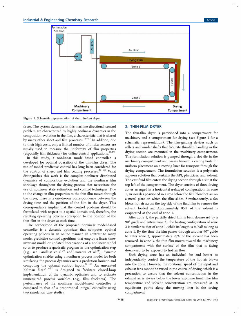
The thin-film dryer is partitioned into a compartment formachinery and a compartment for drying (see Figure 1 for aschematic representation). The film-guiding devices such asrollers and winder shafts that facilitate thin-film handling in thedrying section are mounted in the machinery compartment.The formulation solution is pumped through a slot die in themachinery compartment and passes beneath a casting knife foruniform placement on a moving liner for transport through thedrying compartment. The formulation solution is a polymericaqueous solution that contains the API, plasticizer, and solvent.The cast fluid film enters the drying section through a slit at thetop left of the compartment. The dryer consists of three dryingzones arranged in a horizontal u-shaped configuration. In zone1, air nozzles positioned in a row below the film blow hot air ona metal plate on which the film slides. Simultaneously, a fanblows hot air across the top side of the fluid film to remove thesolvent loaded air. Approximately 85% of the solvent isevaporated at the end of zone 1.After zone 1, the partially dried film is bent downward by a

90° guide and enters zone 2. The heating configuration of zone2 is similar to that of zone 1, while its length is as half as long aszone 1. By the time the film passes through another 90° guideto enter zone 3, approximately 95% of the solvent has beenremoved. In zone 3, the thin film moves toward the machinerycompartment with the surface of the film that is facingdownward to be exposed to hot air flow.Each drying zone has an individual fan and heater to

independently control the temperature of the hot air blowninto the zone. However, the rotational speed of the input andexhaust fans cannot be varied in the course of drying, which is aprecaution to ensure that the solvent concentration in theexhaust air is always below the lower explosive limit. The filmtemperature and solvent concentration are measured at 18equidistant points along the moving liner in the dryingcompartment.

Figure 1. Schematic representation of the thin-film dryer.

Industrial & Engineering Chemistry Research Article

dx.doi.org/10.1021/ie402837c | Ind. Eng. Chem. Res. 2014, 53, 7447−74607448

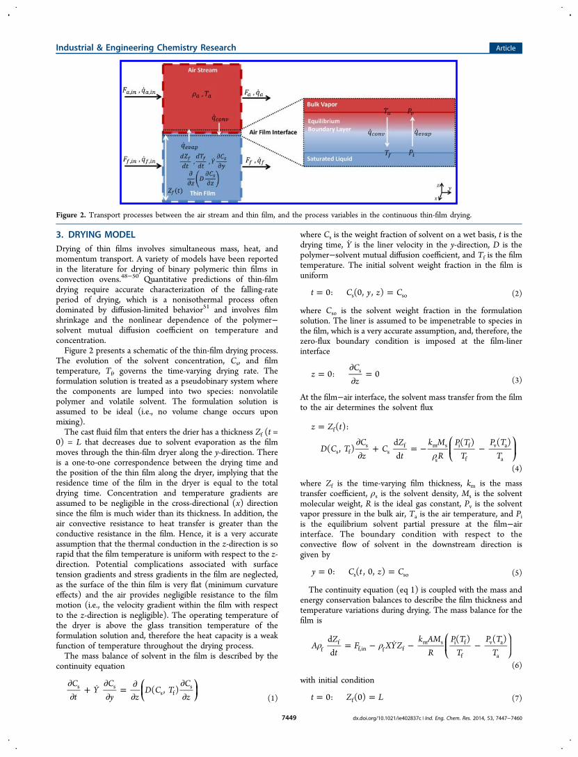
http://pubs.acs.org/action/showImage?doi=10.1021/ie402837c&iName=master.img-000.jpg&w=355&h=224

3. DRYING MODELDrying of thin films involves simultaneous mass, heat, andmomentum transport. A variety of models have been reportedin the literature for drying of binary polymeric thin films inconvection ovens.48−50 Quantitative predictions of thin-filmdrying require accurate characterization of the falling-rateperiod of drying, which is a nonisothermal process oftendominated by diffusion-limited behavior51 and involves filmshrinkage and the nonlinear dependence of the polymer−solvent mutual diffusion coefficient on temperature andconcentration.Figure 2 presents a schematic of the thin-film drying process.

The evolution of the solvent concentration, Cs, and filmtemperature, Tf, governs the time-varying drying rate. Theformulation solution is treated as a pseudobinary system wherethe components are lumped into two species: nonvolatilepolymer and volatile solvent. The formulation solution isassumed to be ideal (i.e., no volume change occurs uponmixing).The cast fluid film that enters the drier has a thickness Zf (t =

0) = L that decreases due to solvent evaporation as the filmmoves through the thin-film dryer along the y-direction. Thereis a one-to-one correspondence between the drying time andthe position of the thin film along the dryer, implying that theresidence time of the film in the dryer is equal to the totaldrying time. Concentration and temperature gradients areassumed to be negligible in the cross-directional (x) directionsince the film is much wider than its thickness. In addition, theair convective resistance to heat transfer is greater than theconductive resistance in the film. Hence, it is a very accurateassumption that the thermal conduction in the z-direction is sorapid that the film temperature is uniform with respect to the z-direction. Potential complications associated with surfacetension gradients and stress gradients in the film are neglected,as the surface of the thin film is very flat (minimum curvatureeffects) and the air provides negligible resistance to the filmmotion (i.e., the velocity gradient within the film with respectto the z-direction is negligible). The operating temperature ofthe dryer is above the glass transition temperature of theformulation solution and, therefore the heat capacity is a weakfunction of temperature throughout the drying process.The mass balance of solvent in the film is described by the

continuity equation

∂∂

+ ∂∂

= ∂∂

∂∂

⎛⎝⎜

⎞⎠⎟

Ct

YCy z

D C TCz

( , )s ss f

s

(1)

where Cs is the weight fraction of solvent on a wet basis, t is thedrying time, Y is the liner velocity in the y-direction, D is thepolymer−solvent mutual diffusion coefficient, and Tf is the filmtemperature. The initial solvent weight fraction in the film isuniform

= =t C y z C0: (0, , )s so (2)

where Cso is the solvent weight fraction in the formulationsolution. The liner is assumed to be impenetrable to species inthe film, which is a very accurate assumption, and, therefore, thezero-flux boundary condition is imposed at the film-linerinterface

=∂∂

=zCz

0: 0s

(3)

At the film−air interface, the solvent mass transfer from the filmto the air determines the solvent flux

ρ

=

∂∂

+ = − −⎛⎝⎜

⎞⎠⎟

z Z t

D C TCz

CZt

k MR

P TT

P TT

( ):

( , )dd

( ) ( )f

s fs

sf m s

s

i f

f

v a

a

(4)

where Zf is the time-varying film thickness, km is the masstransfer coefficient, ρs is the solvent density, Ms is the solventmolecular weight, R is the ideal gas constant, Pv is the solventvapor pressure in the bulk air, Ta is the air temperature, and Piis the equilibrium solvent partial pressure at the film−airinterface. The boundary condition with respect to theconvective flow of solvent in the downstream direction isgiven by

= =y C t z C0: ( , 0, )s so (5)

The continuity equation (eq 1) is coupled with the mass andenergy conservation balances to describe the film thickness andtemperature variations during drying. The mass balance for thefilm is

ρ ρ= − − −⎛⎝⎜

⎞⎠⎟A

Zt

F XYZk AM

RP T

TP T

Tdd

( ) ( )f

ff,in f f

m s i f

f

v a

a

(6)

with initial condition

= =t Z L0: (0)f (7)

Figure 2. Transport processes between the air stream and thin film, and the process variables in the continuous thin-film drying.




where A is the film surface area exposed to air, ρf is the filmdensity, Ff,in is the inlet formulation solution flow rate to thedryer, X is the width of the film, and L is the gap size of thecasting knife.The energy balance for the film includes heat transfer from

the bulk air to the film through an effective heat transfercoefficient as well as evaporation heat of the solvent. Thedescription of film temperature dynamics is simplified by theconduction of heat in the film being fast compared toconvective heat transfer at the film−air interface. The energybalance is

ρ ρ

ρ

+

= − + −

− −⎛⎝⎜

⎞⎠⎟

A c TZt

A c ZTt

h F h XYZ Ak T T

h k AM

RP T

TP T

T

dd

dd

( )

( ) ( )

f p ff

f p ff

f,in f,in f,out f f c a f

fg m s i f

f

v a

a (8)

with initial condition

= =t T T0: (0)f f,in (9)

where cp is the film heat capacity, hf,in is the enthalpy of theformulation solution, hf,out is the enthalpy of the film, kc is theheat transfer coefficient, hfg is the latent heat of vaporization ofsolvent, and Tf,in is the temperature of the formulation solution.In eqs 4, 6, and 8, the vapor pressure of solvent in the bulk

air is considered to be constant throughout the drying process.In contrast, the solvent partial pressure at the film−air interfaceis computed on the basis of the solvent concentration and filmtemperature at the interface using the Flory−Huggins theoryfor phase equilibria.52 The most critical model parameter is thepolymer−solvent mutual diffusion coefficient, which is a strongfunction of solvent concentration and film temperature

=− Φ+ Φ

−γ⎛

⎝⎜⎜

⎞⎠⎟⎟

⎛⎝⎜

⎞⎠⎟D C T D

C

CE

RT( , )

1 ( )

1 ( )exps f 0

p s

p s

a

f (10)

where D0 is the reference mutual diffusion coefficient, Φp is thepolymer volume fraction, γ is a constant, and Ea is the activationenergy.To facilitate the numerical solution of the model equations,

the transformations

ψ =− y YtY (11)

and

η = zZ t( )f (12)

are applied to convert the fixed reference coordinate systeminto a moving reference coordinate system, where Y denotesthe total length of the liner along the three drying zones. Thistransformation not only immobilizes the shrinking film−airinterface with the variable, η, that always has values between 0and 1 but also simplifies numerical solution of the continuity eq1 by eliminating the term for the convective flow of solvent inthe y-direction. The dimensionless forms of the modelequations can be written as

τ η ηη

τ η∂∂

=*

∂∂

∂∂

+*

* ∂∂

⎛⎝⎜

⎞⎠⎟

SZ

DD

SZ

Z S1 dd2

0 (13)

ηη

= ∂∂

=S0: 0

η

η τ ρ

=

*∂∂

+ * = − * −⎛⎝⎜⎜

⎞⎠⎟⎟D

D ZS

SZ Lk M

D C RP T

T TP T

T

1:

dd

( ) ( )

0

m s

0 so s

i f

f,in f

v a

a

ρτ* = − * −

⎛⎝⎜⎜

⎞⎠⎟⎟

DL

Z k MR

P TT T

P TT

dd

( ) ( )f 0 m s i f

f,in f

v a

a (14)

ρτ

ρτ

* *+

* *

= − * − * −⎛⎝⎜⎜

⎞⎠⎟⎟

c Z T D

LT c T T D

LZ

k T T Th k M

RP T

T TP T

T

dd

dd

( )( ) ( )

f p f,in 0 f f p f,in f 0

c a f,in ffg m s i f

f,in f

v a

a

(15)

where the dimensionless variables are

τ = = * =

* =

D tL

SCC

ZZL

TT

T

, , ,

and

02

s

so

f

ff

f,in (16)

and the initial conditions are

τ ψ η= = * =* =

S Z

T

0: (0, , ) 1, (0) 1,

and (0) 1f (17)

The derivation of eq 13 is given in the Appendix. Thetransformation of the reference coordinate system leads toelimination of the terms for the inlet and outlet streams in eqs14 and 15. The physical properties of the polymer−solventsystem and model parameters are listed in Table 1. The latentheat of vaporization hfg (J/kg) is defined by53

= − −h T2502535 2386( 273)fg f (18)

The nonlinear partial differential equation (eq 13) was solvedby the finite volume method. The solution method entailsdiscretization of the spatial variable domain (i.e., η) and the useof the linear upwind difference scheme to approximatederivatives with respect to the spatial variable.54 The thin-filmdrying dynamics can be represented as a set of nonlinearordinary differential equations of the form

= Θ =

= Θ

t t

t

X F X Y U X X

Y H X Y U

( , , , , ), ( ) ,

( , , , , )0 0

(19)

where X(t) = [S Tf* Z*]T is the state vector comprised of thedimensionless solvent weight fraction distributed along the z-direction (one value for each discretization cell), thedimensionless film temperature, and the dimensionless filmthickness; Y(t) is the vector of measured variables includingsolvent weight fraction in the film and film temperature; U(t) isthe vector of system inputs (air temperature Ta); Θ = [km kc γχ]T is the vector of model parameters; F is an algebraic vectorfunction of the dynamic state equations; and H is an algebraicvector function of the measurement equations. The nextsection describes the incorporation of the process model 19into a nonlinear model-based control strategy for the thin-filmdryer.



4. NONLINEAR MODEL-BASED CONTROL APPROACHOptimal operation of drying processes typically aims to reducethe drying time or energy consumption or to enhance the finalproduct quality.55−57 In the thin-film drying process, themechanical characteristics and adhesion properties of themanufactured thin films are greatly affected by the course ofthe drying. Among the critical quality attributes of thin films arethe film thickness and the solvent concentration in the film,which heavily influence the downstream processes of foldingand compaction of the film to form tablets. In addition, thestructural integrity of thin films should be preserved byavoiding defects such as bubbles or cracks, which can form dueto unfavorable film temperatures.The thin-film dryer has three manipulated variablesthe hot

air temperature in each of the three drying zones (See section2). The liner velocity is not used as a manipulated variable inthis study since it is to be employed for optimizing theproduction rate of the thin-film tablet manufacturing processtrain. The solvent weight fraction in the film and the filmtemperature measured at multiple points along the dryer areused for online process control.The controller design problem is formulated in terms of an

optimal control problem. The focus of this study is the startupof the thin-film dryer from the time the film first enters thedryer to when its leading tip first exits the dryer, which is themost challenging problem in the control of the dryer. As will beseen in the Results and Discussion section, the hot airtemperatures in each of the three zones reach their optimalsteady-state values by the end of this startup phase of theoperation. The mathematical formulations enable steering theprocess into a desired operating regime (described by anobjective function) while satisfying various operational andproduct quality constraints. Two control scenarios areconsidered:

• Scenario 1: The objective is to track a predetermined setpoint for the solvent concentration in the exit film whilesatisfying quality constraints on the thickness and structuralintegrity of thin films. The associated optimal control problemis

∫ −

≤ ≤ =

≤ =

≤ ×

< ∀ ∈

−

C C t

T i

T

ti

Z

P P t t

min ( ) d

subject to: eq (19)

303.15 K 348.15 K, 1, 2, 3

d

d5.00 K, 1, 2, 3

4.25 10 m

, [0, ]

t

t

i

i

Ts s,ref

2

a,

a,

f,exit4

b d

a

d

(20)

where Ta = [Ta,1 Ta,2 Ta,3]T is the vector of manipulated

variables consisting of hot air temperatures in the three dryingzones, td is the total drying time (which was set to be largeenough for the film to dry; its value would need to be increase ifthe liner velocity Y were reduced), Cs is the average solventweight fraction over the film thickness at the exit of themachine, Cs,ref is the admissible solvent weight fraction in thefilm at the exit of the machine, Zf,exit is the film thickness at theexit of the machine, Pb is the solvent partial pressure at thefilm−liner interface, and P is the operating pressure of thedryer. The inequality constraint Pb < P, which is enforcedeverywhere in the dryer, ensures that the solvent partialpressure at the film-liner interface remains below the operatingpressure of the dryer at all times during drying to avoid bubbleformation in the thin film.58 The optimal control problem eq20 also incorporates an input constraint on the hot airtemperature in each drying zone. Note that the secondinequality constraint in eq 20 enforces minimum and maximumtemperature ramp rates to penalize excessively large controlactions.• Scenario 2: The objective is to minimize the energy

consumption of the thin-film dryer while satisfying qualityconstraints on the solvent weight fraction in the film, the filmthickness, and bubble formation. The optimal control problemis cast as

∑= −

≤ ≤ =

≤ =

≤

≤ ×

< ∀ ∈

=

−

Q A k T T

T i

T

ti

C

Z

P P t t

min ( )

subject to: eq (19)

303.15 K 348.15 K, 1, 2, 3

d

d5.00 K, 1, 2, 3

0.05 kg solvent/kg film

4.00 10 m

, [0, ]

iT air1

3

a c,a a,i a,in

a,i

a,i

s

f,exit4

b d

a

(21)

where Qair is the energy supplied to the heaters to heat the hotair streams, Aa is the heat exchange surface area of the heaters

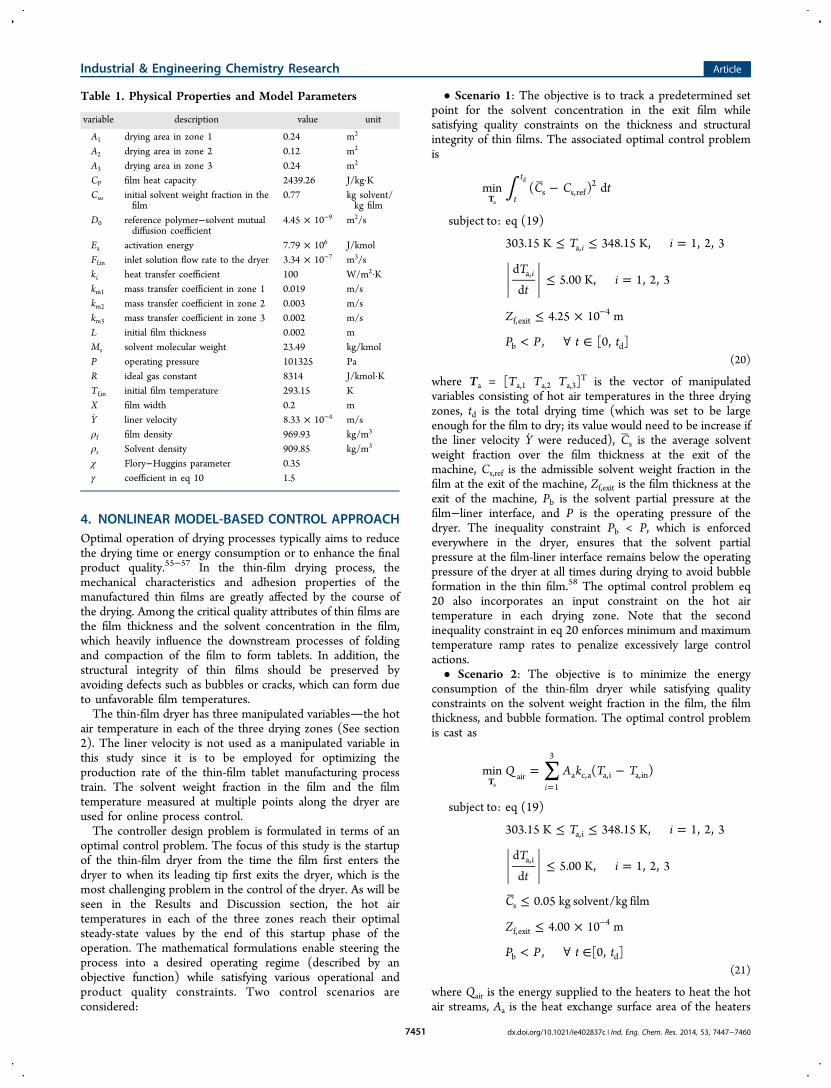
Table 1. Physical Properties and Model Parameters

variable description value unit

A1 drying area in zone 1 0.24 m2



CP film heat capacity 2439.26 J/kg·KCso initial solvent weight fraction in the

film0.77 kg solvent/

kg filmD0 reference polymer−solvent mutual

diffusion coefficient4.45 × 10−9 m2/s

Ea activation energy 7.79 × 106 J/kmolFf,in inlet solution flow rate to the dryer 3.34 × 10−7 m3/skc heat transfer coefficient 100 W/m2·Kkm1 mass transfer coefficient in zone 1 0.019 m/skm2 mass transfer coefficient in zone 2 0.003 m/skm3 mass transfer coefficient in zone 3 0.002 m/sL initial film thickness 0.002 mMs solvent molecular weight 23.49 kg/kmolP operating pressure 101325 PaR ideal gas constant 8314 J/kmol·KTf,in initial film temperature 293.15 KX film width 0.2 mY liner velocity 8.33 × 10−4 m/sρf film density 969.93 kg/m3

ρs Solvent density 909.85 kg/m3

χ Flory−Huggins parameter 0.35γ coefficient in eq 10 1.5



used to heat the inlet air, kc,a is the heat transfer coefficient ofair, and Ta,in is the inlet air temperature. Like eq 20, theinequality constraint Pb < P is enforced along the dryer.To circumvent performance degradation of the optimal

operating policies due to model imperfections and processdisturbances, the underlying model in the optimal controlproblem should be continually updated using process measure-ments. Figure 3 shows the inclusion of the estimator in the

output feedback control structure adopted for real-time controlof the thin-film dryer. As in the model predictive control ofbatch processes,32,59−61 the optimal control problem given byeither eq 20 or 21 is solved online in a shrinking horizon mode.The optimal input sequences are recomputed at each samplingtime instant, when new process measurements becomeavailable, by solving the optimal control problem over a finitetime frame the prediction horizon. The prediction horizonshrinks as the thin film moves toward the exit of the dryer. As intraditional receding horizon control, only the first computedtime instance of each optimal input sequence is applied to theprocess at each sampling time instant.The output feedback structure in Figure 3 necessitates

recursive initialization of the dynamic optimizer at eachsampling time instant. This initialization is performed by anunscented Kalman filter (UKF)41,42 that uses the processmodel, along with online measurements, to construct theprofile of state variables. Unscented Kalman filtering is aderivative-free state estimation technique that avoids lineariza-

tion of the process model through an unscented trans-formation, while being computationally inexpensive (see thework of Mesbah et al.47 for further discussion and a numericalstudy that compares UKF with other state estimators).Recursive initialization of the dynamic optimizer in thefeedback control structure compensates for model imperfec-tions and process disturbances to a large extent. In addition, thestate estimator enables estimation of process variables such asfilm thickness that cannot be measured online due totechnological or economic limitations.To solve the optimal control problem, the infinite-dimen-

sional problem is converted into a finite-dimensional nonlinearprogram (NLP) using the direct single shooting optimizationstrategy.62 The single shooting optimizer is implemented inMATLAB where the model equations (a set of highly nonlinearstiff ordinary differential equations) and the NLP aresequentially solved by ode15s and fmincon, respectively. In theUKF, the deterministically chosen sigma points are selectedsymmetrically around the a priori state vector with a distance ofthe square root of the covariance.63 As shown in Figure 3, thecontrol strategy is applied to a plant simulator of the dynamicsof the thin-film dryer, which exploits a nonlinear process modelidentical to that used in the UKF and the dynamic optimizer.The process measurements are corrupted by random noisesequences having normal distributions. The measurements aresampled every 200 s.The performance of the model-based control strategy is

evaluated with respect to a classical control strategy consistingof a proportional integral (PI) controller to regulate theconcentration of solvent remaining in the film. The parametersof the PI controller are determined by characterizing the open-loop system dynamics and applying the internal model control(IMC) tuning rules for a first-order-plus-dead-time system.64 Inthe classical control approach, a soft sensor is designed forprocess monitoring to estimate the unmeasured film thicknessin the absence of accurate online measurement sensor. The softsensor consists of the nonlinear process model (eq 19), whichis solved in parallel with the real process by using the sameinput U as that applied to the process. The soft sensor isinitialized recursively at regular time intervals when measure-ments become available. Like the UKF, the soft sensor

Figure 3. Nonlinear model-based control approach applied to the thin-film dryer.

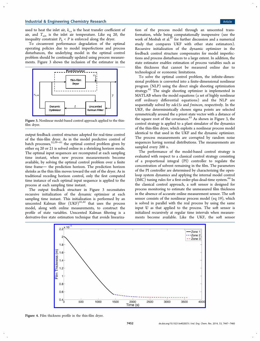
Figure 4. Film thickness profile in the thin-film dryer.



http://pubs.acs.org/action/showImage?doi=10.1021/ie402837c&iName=master.img-002.png&w=199&h=108


estimates the unmeasured film thickness by using the filmtemperature and solvent concentration measurements, whichare obtained at equidistant points along the moving liner in thedrying compartment (see section 2).

5. RESULTS AND DISCUSSION5.1. Process Dynamics. This section explores the open-

loop dynamics of the thin-film dryer. The manipulatedvariables the hot air temperatures in the three dryingzonesare initially set to 333.15 K (the initial and operatingconditions are given in Table 1). Figure 4 shows the evolutionof the film thickness in the course of the drying. The thicknessof the fluid film is reduced significantly in zone 1 and to a lesserextent in zones 2 and 3. These reductions are associated withrapid solvent evaporation in zone 1, which leads to a steepdecrease in the average solvent weight fraction in the film (seeFigure 5).Initially, the thin-film drying is limited primarily by external

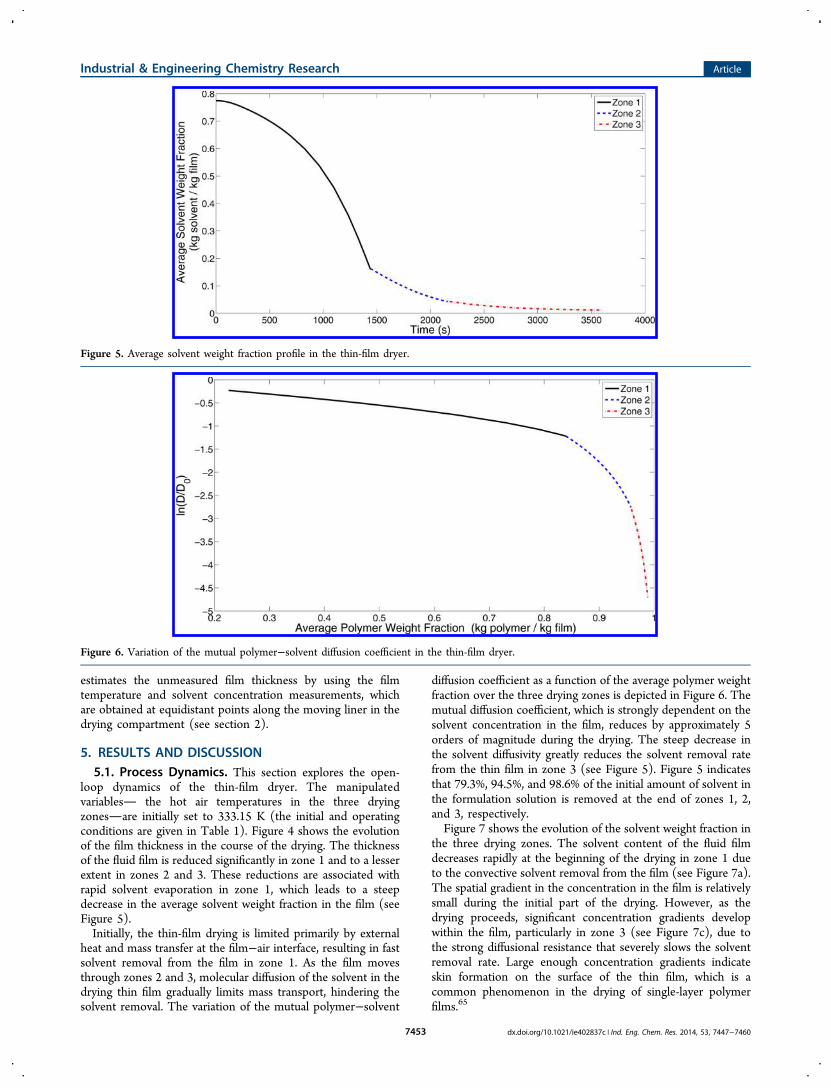
heat and mass transfer at the film−air interface, resulting in fastsolvent removal from the film in zone 1. As the film movesthrough zones 2 and 3, molecular diffusion of the solvent in thedrying thin film gradually limits mass transport, hindering thesolvent removal. The variation of the mutual polymer−solvent

diffusion coefficient as a function of the average polymer weightfraction over the three drying zones is depicted in Figure 6. Themutual diffusion coefficient, which is strongly dependent on thesolvent concentration in the film, reduces by approximately 5orders of magnitude during the drying. The steep decrease inthe solvent diffusivity greatly reduces the solvent removal ratefrom the thin film in zone 3 (see Figure 5). Figure 5 indicatesthat 79.3%, 94.5%, and 98.6% of the initial amount of solvent inthe formulation solution is removed at the end of zones 1, 2,and 3, respectively.Figure 7 shows the evolution of the solvent weight fraction in

the three drying zones. The solvent content of the fluid filmdecreases rapidly at the beginning of the drying in zone 1 dueto the convective solvent removal from the film (see Figure 7a).The spatial gradient in the concentration in the film is relativelysmall during the initial part of the drying. However, as thedrying proceeds, significant concentration gradients developwithin the film, particularly in zone 3 (see Figure 7c), due tothe strong diffusional resistance that severely slows the solventremoval rate. Large enough concentration gradients indicateskin formation on the surface of the thin film, which is acommon phenomenon in the drying of single-layer polymerfilms.65

Figure 5. Average solvent weight fraction profile in the thin-film dryer.

Figure 6. Variation of the mutual polymer−solvent diffusion coefficient in the thin-film dryer.





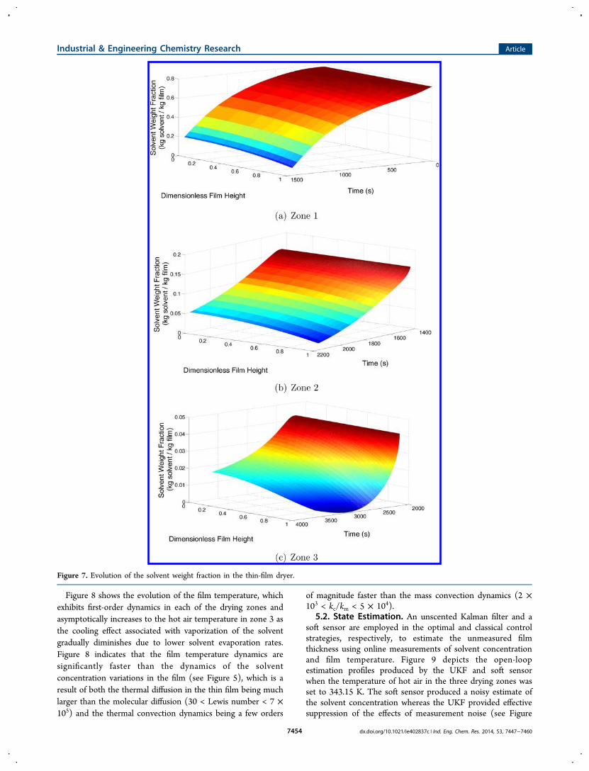
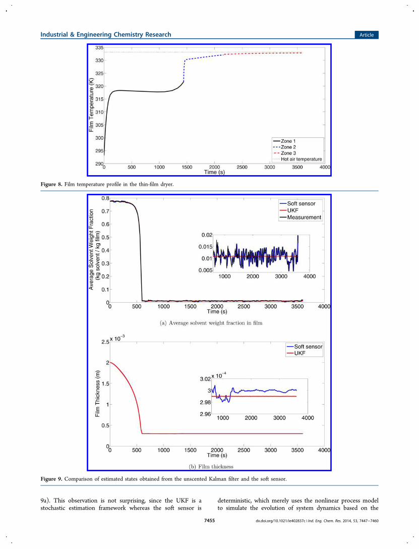
Figure 8 shows the evolution of the film temperature, whichexhibits first-order dynamics in each of the drying zones andasymptotically increases to the hot air temperature in zone 3 asthe cooling effect associated with vaporization of the solventgradually diminishes due to lower solvent evaporation rates.Figure 8 indicates that the film temperature dynamics aresignificantly faster than the dynamics of the solventconcentration variations in the film (see Figure 5), which is aresult of both the thermal diffusion in the thin film being muchlarger than the molecular diffusion (30 < Lewis number < 7 ×105) and the thermal convection dynamics being a few orders

of magnitude faster than the mass convection dynamics (2 ×103 < kc/km < 5 × 104).

5.2. State Estimation. An unscented Kalman filter and asoft sensor are employed in the optimal and classical controlstrategies, respectively, to estimate the unmeasured filmthickness using online measurements of solvent concentrationand film temperature. Figure 9 depicts the open-loopestimation profiles produced by the UKF and soft sensorwhen the temperature of hot air in the three drying zones wasset to 343.15 K. The soft sensor produced a noisy estimate ofthe solvent concentration whereas the UKF provided effectivesuppression of the effects of measurement noise (see Figure

Figure 7. Evolution of the solvent weight fraction in the thin-film dryer.




9a). This observation is not surprising, since the UKF is astochastic estimation framework whereas the soft sensor is

deterministic, which merely uses the nonlinear process modelto simulate the evolution of system dynamics based on the

Figure 8. Film temperature profile in the thin-film dryer.

Figure 9. Comparison of estimated states obtained from the unscented Kalman filter and the soft sensor.





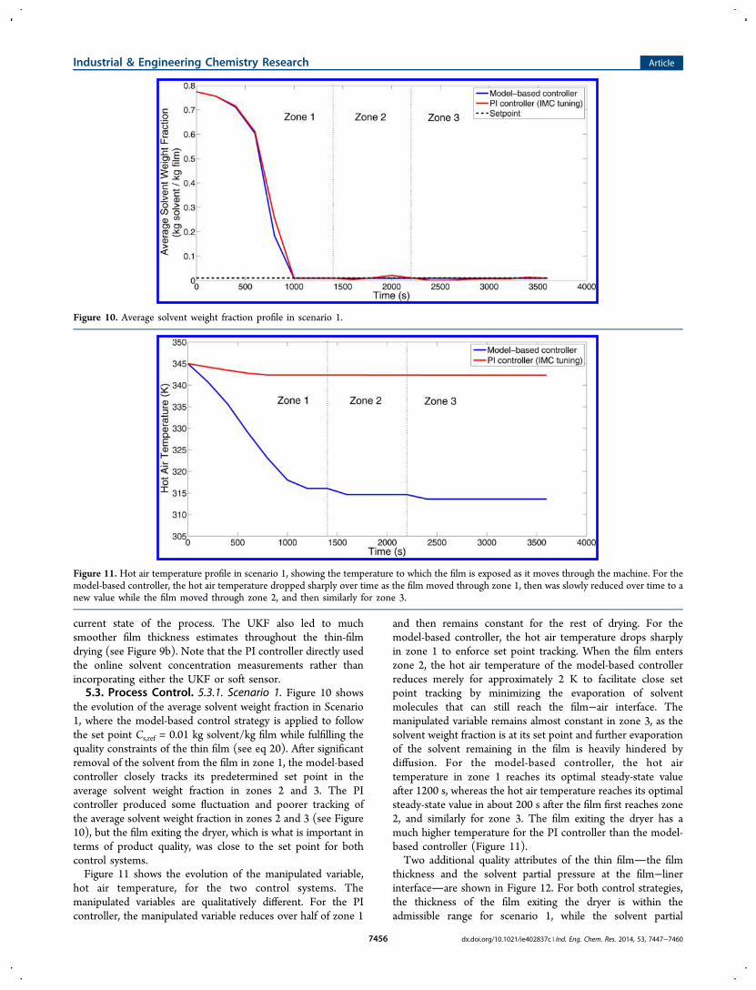
current state of the process. The UKF also led to muchsmoother film thickness estimates throughout the thin-filmdrying (see Figure 9b). Note that the PI controller directly usedthe online solvent concentration measurements rather thanincorporating either the UKF or soft sensor.5.3. Process Control. 5.3.1. Scenario 1. Figure 10 shows

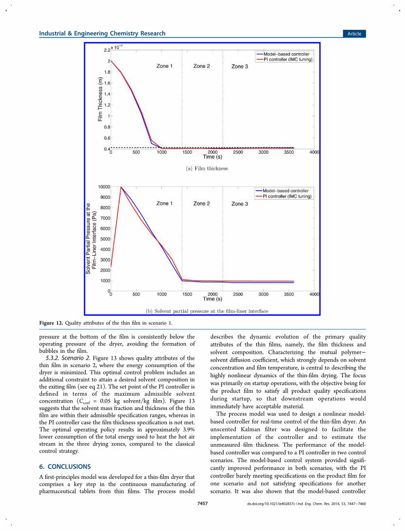
the evolution of the average solvent weight fraction in Scenario1, where the model-based control strategy is applied to followthe set point Cs,ref = 0.01 kg solvent/kg film while fulfilling thequality constraints of the thin film (see eq 20). After significantremoval of the solvent from the film in zone 1, the model-basedcontroller closely tracks its predetermined set point in theaverage solvent weight fraction in zones 2 and 3. The PIcontroller produced some fluctuation and poorer tracking ofthe average solvent weight fraction in zones 2 and 3 (see Figure10), but the film exiting the dryer, which is what is important interms of product quality, was close to the set point for bothcontrol systems.Figure 11 shows the evolution of the manipulated variable,

hot air temperature, for the two control systems. Themanipulated variables are qualitatively different. For the PIcontroller, the manipulated variable reduces over half of zone 1

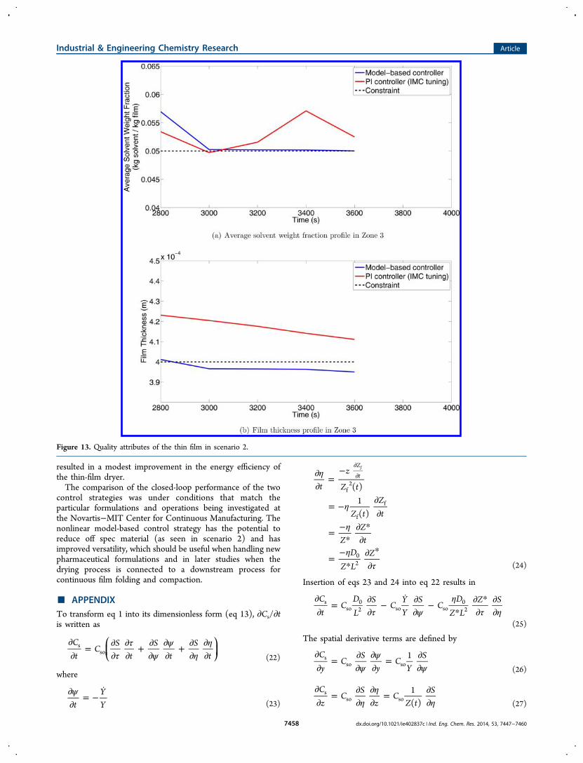
and then remains constant for the rest of drying. For themodel-based controller, the hot air temperature drops sharplyin zone 1 to enforce set point tracking. When the film enterszone 2, the hot air temperature of the model-based controllerreduces merely for approximately 2 K to facilitate close setpoint tracking by minimizing the evaporation of solventmolecules that can still reach the film−air interface. Themanipulated variable remains almost constant in zone 3, as thesolvent weight fraction is at its set point and further evaporationof the solvent remaining in the film is heavily hindered bydiffusion. For the model-based controller, the hot airtemperature in zone 1 reaches its optimal steady-state valueafter 1200 s, whereas the hot air temperature reaches its optimalsteady-state value in about 200 s after the film first reaches zone2, and similarly for zone 3. The film exiting the dryer has amuch higher temperature for the PI controller than the model-based controller (Figure 11).Two additional quality attributes of the thin filmthe film

thickness and the solvent partial pressure at the film−linerinterfaceare shown in Figure 12. For both control strategies,the thickness of the film exiting the dryer is within theadmissible range for scenario 1, while the solvent partial

Figure 10. Average solvent weight fraction profile in scenario 1.

Figure 11. Hot air temperature profile in scenario 1, showing the temperature to which the film is exposed as it moves through the machine. For themodel-based controller, the hot air temperature dropped sharply over time as the film moved through zone 1, then was slowly reduced over time to anew value while the film moved through zone 2, and then similarly for zone 3.





pressure at the bottom of the film is consistently below theoperating pressure of the dryer, avoiding the formation ofbubbles in the film.5.3.2. Scenario 2. Figure 13 shows quality attributes of the

thin film in scenario 2, where the energy consumption of thedryer is minimized. This optimal control problem includes anadditional constraint to attain a desired solvent composition inthe exiting film (see eq 21). The set point of the PI controller isdefined in terms of the maximum admissible solventconcentration (Cs,ref = 0.05 kg solvent/kg film). Figure 13suggests that the solvent mass fraction and thickness of the thinfilm are within their admissible specification ranges, whereas inthe PI controller case the film thickness specification is not met.The optimal operating policy results in approximately 3.9%lower consumption of the total energy used to heat the hot airstream in the three drying zones, compared to the classicalcontrol strategy.

6. CONCLUSIONS

A first-principles model was developed for a thin-film dryer thatcomprises a key step in the continuous manufacturing ofpharmaceutical tablets from thin films. The process model

describes the dynamic evolution of the primary qualityattributes of the thin films, namely, the film thickness andsolvent composition. Characterizing the mutual polymer−solvent diffusion coefficient, which strongly depends on solventconcentration and film temperature, is central to describing thehighly nonlinear dynamics of the thin-film drying. The focuswas primarily on startup operations, with the objective being forthe product film to satisfy all product quality specificationsduring startup, so that downstream operations wouldimmediately have acceptable material.The process model was used to design a nonlinear model-

based controller for real-time control of the thin-film dryer. Anunscented Kalman filter was designed to facilitate theimplementation of the controller and to estimate theunmeasured film thickness. The performance of the model-based controller was compared to a PI controller in two controlscenarios. The model-based control system provided signifi-cantly improved performance in both scenarios, with the PIcontroller barely meeting specifications on the product film forone scenario and not satisfying specifications for anotherscenario. It was also shown that the model-based controller

Figure 12. Quality attributes of the thin film in scenario 1.




resulted in a modest improvement in the energy efficiency ofthe thin-film dryer.The comparison of the closed-loop performance of the two

control strategies was under conditions that match theparticular formulations and operations being investigated atthe Novartis−MIT Center for Continuous Manufacturing. Thenonlinear model-based control strategy has the potential toreduce off spec material (as seen in scenario 2) and hasimproved versatility, which should be useful when handling newpharmaceutical formulations and in later studies when thedrying process is connected to a downstream process forcontinuous film folding and compaction.

■ APPENDIXTo transform eq 1 into its dimensionless form (eq 13), ∂Cs/∂tis written as

ττ

ψψ

ηη∂

∂= ∂

∂∂∂

+ ∂∂

∂∂

+ ∂∂

∂∂

⎛⎝⎜

⎞⎠⎟

Ct

CS

tS

tS

ts

so(22)

where

ψ∂∂

= −

tYY (23)

η

η

η

ητ

∂∂

=−

= −∂∂

= −*

∂ *∂

=−

*∂ *∂

∂∂

t

z

Z t

Z tZt

ZZt

DZ L

Z

( )1( )

Z

t

f2

f

f

02

f

(24)

Insertion of eqs 23 and 24 into eq 22 results in

τ ψη

τ η∂∂

= ∂∂

− ∂

∂−

*∂ *∂

∂∂

Ct

CDL

SC

YY

SC

DZ L

Z Ssso

02 so so

02

(25)

The spatial derivative terms are defined by

ψψ

ψ∂∂

= ∂∂

∂∂

= ∂∂

Cy

CS

yC

YS1s

so so(26)

ηη

η∂∂

= ∂∂

∂∂

= ∂∂

Cz

CS

zC

Z tS1

( )s

so so(27)

Figure 13. Quality attributes of the thin film in scenario 2.




Substitution of eqs 25−27 into eq 1 leads to eq 13.

■ AUTHOR INFORMATION

Corresponding Author*E-mail: [email protected].

NotesThe authors declare no competing financial interest.

■ ACKNOWLEDGMENTS

Novartis Pharma AG is acknowledged for financial support.

■ REFERENCES(1) Leuenberger, H. New Trends in the Production ofPharmaceutical Granules: Batch Versus Continuous Processing. Eur.J. Pharm. Biopharm. 2001, 52, 289−296.(2) McKenzie, P.; Kiang, S.; Tom, J.; Rubin, A. E.; Futran, M. CanPharmaceutical Process Development Become High Tech? AIChE J.2006, 52, 3990−3994.(3) Plumb, K. Continuous Processing in the Pharmaceutical Industry:Changing the Mind Set. Chem. Eng. Res. Des. 2005, 83, 730−738.(4) Schaber, S. D.; Gerogiorgis, D. I.; Ramachandran, R.; Evans, J. M.B.; Barton, P. I.; Trout, B. L. Economic Analysis of IntegratedContinuous and Batch Pharmaceutical Manufacturing: A Case Study.Ind. Eng. Chem. Res. 2011, 50, 10083−10092.(5) Kockmann, N.; Gottsponer, M.; Zimmermann, B.; Roberge, D.M. Enabling Continuous Flow Chemistry in Microstructured Devicesfor Pharmaceutical and Fine Chemical Production. Chem.Eur. J.2008, 14, 7470−7477.(6) Blanco, M.; Alcala, M. Content Uniformity and Tablet HardnessTesting of Intact Pharmaceutical Tablets by Near Infrared Spectros-copy: A Contribution to Process Analytical Technologies. Anal. Chim.Acta 2006, 557, 353−359.(7) Yu, L. Pharmaceutical Quality by Design: Product and ProcessDevelopment, Understanding, and Control. Pharm. Res. 2008, 25,781−791.(8) Du, Y.; Luna, L. E.; Chadwick, K.; Kim, K. T.; Xi, L.; Myerson, A.S.; Trout, B. L. A Novel Thin Film-Based Pharmaceutical TabletManufacturing Process: Formulation, Processing, and Properties.2013, submitted for publication.(9) Dinge, A.; Nagarsenker, M. Formulation and Evaluation of FastDissolving Films for Delivery of Triclosan to the Oral Cavity. AAPSPharmSciTech 2008, 9, 349−356.(10) Hirani, J. J.; Rathod, D. A.; Vadalia, K. R. Orally DisintegratingTablets: A Review. Trop. J. Pharm. Res. 2009, 8, 161−172.(11) Kunte, S.; Tandale, P. Fast Dissolving Strips: A Novel Approachfor the Delivery of Verapamil. J. Pharm. BioAllied Sci. 2010, 2, 325−328.(12) Arya, A.; Chandra, A.; Sharma, V.; Pathak, K. Fast DissolvingOral Films: An Innovative Drug Delivery System and Dosage Form.Int. J. ChemTech Res. 2010, 2, 576−583.(13) VanAntwerp, J. G.; Featherstone, A. P.; Braatz, R. D.;Ogunnaike, B. A. Cross-directional Control of Sheet and FilmProcesses. Automatica 2007, 43, 191−211.(14) Lindeborg, C. A Simulation Study of the Moisture Cross-directional Control Problem. In Instrumentation and Automation in thePaper, Rubber, Plastics, and Polymerization Industries; Kaya, A.,Williams, T. J., Eds.; Pergamon Press: Oxford, U.K., 1986; pp 59−64.(15) Kjaer, A. P.; Wellstead, P. E.; Heath, W. P. On-Line Sensing ofPaper Machine Wet-End Properties: Dry Line Detector. IEEE Trans.Control Sys. Technol. 1997, 5, 571−585.(16) Vyse, R.; Hagart-Alexander, C.; Heaven, M.; Steele, T.; Chase,L.; Goss, J.; Preston, J. High Speed Full Cross Direction ProfileMeasurements and Control for the Paper Machine Wet End.Proceedings of the 52nd APPITA Annual General Conference, Carlton,Australia, May 11−14, 1998; pp 435−442.

(17) Poirier, D.; Vyse, R.; Hagart-Alexander, C.; Heaven, M.;Ghofraniha, J. New Trends in CD Weight Control for Multi-PlyApplications. Pap. Technol. Ind. 1999, 40, 41−50.(18) Toensmeier, P. A. Sensor Scans 1000 Sites at 10 in./sec. Mod.Plast. 1991, 68, 35−37.(19) Shelley, P. H.; Booksh, K. S.; Burgess, L. W.; Kowalski, B. R.Polymer Film Thickness Determination with a High PrecisionScanning Reflectometer. Appl. Spectrosc. 1996, 50, 119−125.(20) Bergh, L. G.; Macgregor, J. F. Spatial Control of Sheet and FilmForming Processes. Can. J. Chem. Eng. 1987, 65, 148−155.(21) Braatz, R. D.; Tyler, M. L.; Morari, M.; Pranckh, F. R.; Sartor, L.Identification and Cross-Directional Control of Coating Processes.AIChE J. 1992, 38, 1329−1339.(22) Halouskova, A.; Karny, M.; Nagy, I. Adaptive Cross-directionalControl of Paper Basis Weight. Automatica 1993, 29, 425−429.(23) Tyler, M. L.; Morari, M. Estimation of Cross-DirectionalProperties: Scanning vs. Stationary Sensors. AIChE J. 1995, 41, 846−854.(24) Rawlings, J. B.; Chien, I. L. Gage Control of Film and Sheet-Forming Processes. AIChE J. 1996, 42, 753−766.(25) Heath, W. P. Orthogonal Functions for Cross DirectionalControl of Web Forming Processes. Automatica 1996, 32, 183−198.(26) Rao, C. V.; Campbell, J. C.; Rawlings, J. B.; Wright, S. J. EfficientImplementation of Model Predictive Control for Sheet and FilmForming Processes. Proceedings of the American Control Conference,Albuquerque, NM, June 1997; pp 2940−2944.(27) Rigopoulos, A.; Arkun, Y.; Kayihan, F. Model Predictive Controlof CD Profiles in Sheet Forming Processes Using Full ProfileDisturbance Models Identified by Adaptive PCA. Proceedings of theAmerican Control Conference; Albuquerque, NM, June 1997; pp 1468−1472.(28) Campbell, J. C.; Rawlings, J. B. Predictive Control of Sheet- andFilm-Forming Processes. AIChE J. 1998, 44, 1713−1723.(29) VanAntwerp, J. G.; Braatz, R. D. Fast Model Predictive Controlof Sheet and Film Processes. IEEE Trans. Control Sys. Technol. 2000, 8,408−417.(30) Landlust, J.; Mesbah, A.; Wildenberg, J.; Kalbasenka, A. N.;Kramer, H. J. M.; Ludlage, J. H. A. An Industrial Model PredictiveControl Architecture for Batch Crystallization. Proceedings of the 17thInternational Symposium on Industrial Crystallization, Maastricht, TheNetherlands, Sep 14−17, 2008; pp 35−42.(31) Daraoui, N.; Dufour, P.; Hammouri, H.; Hottot, A. ModelPredictive Control During the Primary Drying Stage of Lyophilisation.Control Eng. Pract. 2010, 18, 483−494.(32) Eaton, J. W.; Rawlings, J. B. Feedback Control of ChemicalProcesses Using On-Line Optimization Techniques. Comput. Chem.Eng. 1990, 14, 469−479.(33) Chung, S. H.; Ma, D. L.; Braatz, R. D. Optimal Seeding in BatchCrystallization. Can. J. Chem. Eng. 1999, 77, 590−596.(34) Biegler, L. T. Efficient Solution of Dynamic Optimization andNMPC Problems. In Nonlinear Model Predictive Control; Allgower, F.,Zheng, A., Eds.; Springer: Basel, Switzerland, 2000; pp 219−243.(35) Qin, S. J.; Badgwell, T. A. An Overview of Nonlinear ModelPredictive Control Applications. In Nonlinear Model Predictive Control;Allgower, F., Zheng, A., Eds.; Springer: Basel, Switzerland, 2000; p369−392.(36) Binder, T.; Blank, L.; Bock, H.; Bulirsch, R.; Dahmen, W.; Diehl,M.; Kronseder, T.; Marquardt, W.; Schloder, J. P.; Strykr, O. V.Introduction to Model Based Optimization of Chemical Processes onMoving Horizons. In Online Optimization of Large Scale Systems;Grotchel, M., Krumke, S. O., Rambau, J., Eds.; Springer: Berlin, 2001;pp 295−340.(37) Sheikhzadeh, M.; Trifkovic, M.; Rohani, S. Real-Time OptimalControl of an Anti-Solvent Isothermal Semi-Batch CrystallizationProcess. Chem. Eng. Sci. 2007, 63, 829−839.(38) Simon, L. L.; Nagy, Z. K.; Hungerbuhler, K. Model BasedControl of a Liquid Swelling Constrained Batch Reactor Subject toRecipe Uncertainties. Chem. Eng. J. 2009, 153, 151−158.



mailto:[email protected]

(39) Mesbah, A.; Huesman, A. E. M.; Kramer, H. J. M.; Nagy, Z. K.;Van den Hof, P. M. J. Real-Time Control of a Semi-Industrial Fed-Batch Evaporative Crystallizer Using Different Direct OptimizationStrategies. AIChE J. 2011, 57, 1557−1569.(40) Mesbah, A.; Nagy, Z. K.; Huesman, A. E. M.; Kramer, H. J. M.;Van den Hof, P. M. J. Nonlinear Model-based Control of a Semi-industrial Batch Crystallizer using a Population Balance ModelingFramework. IEEE Trans. Control Sys. Technol. 2012, 20, 1188−1201.(41) Julier, S. J.; Uhlmann, J. K. A New Extension of the KalmanFilter to Nonlinear Systems. Proceedings of the 11th InternationalSymposium on Aerospace/Defense Sensing, Simulation and Controls,Orlando, FL, April 1997; pp 182−193.(42) Julier, S. J.; Uhlmann, J. K. Unscented Filtering and NonlinearEstimation. Proc. IEEE 2004, 92, 401−422.(43) Romanenko, A.; Santos, L. O.; Afonso, P. A. Unscented KalmanFiltering of a Simulated pH System. Ind. Eng. Chem. Res. 2004, 43,7531−7538.(44) Schei, T. S. On-Line Estimation for Process Control andOptimization Applications. J. Process Control 2008, 18, 821−828.(45) Hermanto, M. W.; Chiu, M. S.; Braatz, R. D. Nonlinear ModelPredictive Control for the Polymorphic Transformation of L-GlutamicAcid Crystals. AIChE J. 2009, 55, 2631−2645.(46) Mangold, M.; Buck, A.; Schenkendorf, R.; Steyer, C.; Voigt, A.;Sundmacher, K. Two State Estimators for the Barium SulfatePrecipitation in a Semi-Batch Reactor. Chem. Eng. Sci. 2009, 64,646−660.(47) Mesbah, A.; Huesman, A. E. M.; Kramer, H. J. M.; Van den Hof,P. M. J. A Comparison of Nonlinear Observers for Output FeedbackModel-Based Control of Seeded Batch Crystallization Processes. J.Process Control 2011, 21, 652−666.(48) Vrentas, J. S.; Vrentas, C. M. Drying of Solvent-Coated PolymerFilms. J. Polym. Sci., Part B: Polym. Phys. 1994, 32, 187−194.(49) Alsoy, S.; Duda, J. L. Drying of Solvent Coated Polymer Films.Drying Technol. 1998, 16, 15−44.(50) Pakowski, Z.; Mujumdar, A. S. In Handbook of Industrial Drying;Mujumdar, A. S., Ed.; CRC Press: Boca Raton, FL, 2006; p 53−80.(51) Price, P. E.; Wang, S.; Romdhane, I. H. Extracting EffectiveDiffusion Parameters from Drying Experiments. AIChE J. 1997, 43,1925−1934.(52) Fried, J. R. Polymer Science & Technology; Prentice Hall: UpperSaddle River, NJ, 2003.(53) Brooker, D. B. Mathematical Model of the Psychrometric Chart.Trans. ASABE 1967, 10, 558−560.(54) Leveque, R. J. Finite Volume Methods for Hyperbolic Problems;Cambridge University Press: Cambridge, U.K., 2002.(55) Barttfeld, M.; Alleborn, N.; Durst, F. Dynamic Optimization ofMultiple-Zone Air Impingement Drying Process. Comput. Chem. Eng.2006, 30, 467−489.(56) Dufour, P. Control Engineering in Drying Technology: Reviewand Trends. Drying Technol. 2006, 24, 889−904.(57) Allanic, N.; Salagnac, P.; Glouannec, P. Optimal ConstrainedControl of an Infrared-Convective Drying of a Polymer AqueousSolution. Chem. Eng. Res. Des. 2009, 87, 908−914.(58) Price, P. E.; Cairncross, R. A. Optimization of Single-ZoneDrying of Polymer Solution Coatings using Mathematical Modeling. J.Appl. Polym. Sci. 2000, 78, 149−165.(59) Thomas, M. M.; Kardos, J. L.; Joseph, B. Shrinking HorizonModel Predictive Control Applied to Autoclave Curing of CompositeLaminate Materials. Proceedings of the American Control Conference,Baltimore, MD, June 29−July 1, 1994; pp 505−510.(60) Brosilow, C.; Joseph, B. Techniques of Model-based Control;Prentice Hall: Upper Saddle River, NJ, 2002.(61) Diehl, M.; Ferreau, H. J.; Haverbeke, N. In Nonlinear ModelPredictive Control: Towards New Challenging Applications; Magni, L.,Raimondo, D. M., Allgower, F., Eds.; Springer: Berlin, 2009; pp 391−417.(62) Biegler, L.; Cuthrell, J. Improved Infeasible Path Optimizationfor Sequential Modular Simulators II: The Optimization Algorithm.Comput. Chem. Eng. 1985, 9, 257−267.

(63) van der Merwe, R.; Wan, E. The Square-Root UnscentedKalman Filter for State and Parameter Estimation. Proceedings of IEEEInternational Conference on Acoustics, Speech and Signal Processing, SaltLake City, UT, May 7−11, 2001; pp 3461−3464(64) Rivera, D. E.; Morari, M.; Skogestad, S. Internal Model Control.4. PID Controller Design. Ind. Eng. Chem. Process Des. Dev. 1986, 25,252−265.(65) Alsoy, S.; Duda, J. L. Modeling of Multilayer Drying of PolymerFilms. J. Polym. Sci., Part B: Polym. Phys. 1999, 16, 1665−1674.



Documents

Nonlinear Model-Based Control of Thin-Film Drying for ...web.mit.edu/braatzgroup/nonlinear_model_based_control_of_thin_film... · Nonlinear Model-Based Control of Thin-Film Drying