Embed Size (px)
Citation preview

JOURNAL OF GEOPHYSICAL RESEARCH, VOL. ???, XXXX, DOI:10.1029/,
Nonlinear force-free modeling of the solar coronal magnetic fieldT. WiegelmannMax-Planck-Institut fur Sonnensystemforschung, Max-Planck-Strasse 2, 37191 Katlenburg-Lindau, Germany
Abstract. The coronal magnetic field is an important quantity because the magneticfield dominates the structure of the solar corona. Unfortunately direct measurements ofcoronal magnetic fields are usually not available. The photospheric magnetic field is mea-sured routinely with vector magnetographs. These photospheric measurements are ex-trapolated into the solar corona. The extrapolated coronal magnetic field depends on as-sumptions regarding the coronal plasma, e.g. force-freeness. Force-free means that all non-magnetic forces like pressure gradients and gravity are neglected. This approach is welljustified in the solar corona due to the low plasma beta. One has to take care, however,about ambiguities, noise and non-magnetic forces in the photosphere, where the mag-netic field vector is measured. Here we review different numerical methods for a nonlin-ear force-free coronal magnetic field extrapolation: Grad-Rubin codes, upward integra-tion method, MHD-relaxation, optimization and the boundary element approach. We brieflydiscuss the main features of the different methods and concentrate mainly on recentlydeveloped new codes.
Contents
1. Introduction
1.1. Why do we need nonlinear force-free fields?
2. Nonlinear force-free codes
2.1. Grad-Rubin method
2.2. Upward integration method
2.3. MHD relaxation
2.4. Optimization approach
2.5. Boundary element or Greens function likemethod
3. How to deal with non-force-free boundaries andnoise ?
3.1. Consistency check of vector magnetograms
3.2. Preprocessing
4. Code testing and code comparisons
4.1. The NLFFF-consortium
5. Conclusions and Outlook
1. IntroductionInformation regarding the coronal magnetic field are im-portant for space weather application like the onset offlares and coronal mass ejections (CMEs). Unfortunatelywe usually cannot measure the coronal magnetic field di-rectly, although recently some progress has been made[see e.g., Judge, 1998; Solanki et al., 2003; Lin et al.,2004]. Due to the optically thin coronal plasma directmeasurements of the coronal magnetic field have a line-of-sight integrated character and to derive the accurate3D structure of the coronal magnetic field a vector to-mographic inversion is required. Corresponding feasibil-ity studies based on coronal Zeeman and Hanle effect
Copyright 2008 by the American Geophysical Union.0148-0227/08/$9.00
1
arX
iv:0
801.
2902
v1 [
astr
o-ph
] 1
8 Ja
n 20
08
X - 2 WIEGELMANN: CORONAL MAGNETIC FIELDS.
measurements have recently been done by Kramar et al.[2006] and Kramar and Inhester [2006]. These directmeasurements are only available for a few individual casesand usually one has to extrapolate the coronal magneticfield from photospheric magnetic measurements. To doso, one has to make assumptions regarding the coronalplasma. It is helpful that the low solar corona is stronglydominated by the coronal magnetic field and the mag-netic pressure is orders of magnitudes higher than theplasma pressure. The quotient of plasma pressure p andmagnetic pressure, B2/(2µ0) is small compared to unity(β = 2µ0p/B
2 1). In lowest order non-magnetic forceslike pressure gradient and gravity can be neglected whichleads to the force-free assumption. Force free fields arecharacterized by the equations:
j×B = 0 (1)
∇×B = µ0j, (2)
∇ ·B = 0, (3)
where B is the magnetic field, j the electric current den-sity and µ0 the permeability of vacuum. Equation (1)implies that for force-free fields the current density andthe magnetic field are parallel, i.e.
µ0j = αB, (4)
or by replacing j with Eq. (2)
∇×B = αB, (5)
where α is called the force-free function. To get someinsights in the structure of the space dependent functionα, we take the divergence of Eq. (4) and make use ofEqs. (2) and (3):
B · ∇α = 0, (6)
which tells us that the force-free function α is con-stant on every field line, but will usually change from onefield line to another. This generic case is called nonlinearforce-free approach.
Popular simplifications are α = 0 (current free poten-tial fields, see e.g., Schmidt [1964]; Semel [1967]; Schat-ten et al. [1969]; Sakurai [1982]) and α = constant (linearforce-free approach, see e.g., Nakagawa and Raadu [1972];Chiu and Hilton [1977]; Seehafer [1978]; Alissandrakis[1981]; Seehafer [1982]; Semel [1988]). These simplifiedmodels have been in particular popular due to their rel-ative mathematical simplicity and because only line-of-sight photospheric magnetic field measurements are re-quired. Linear force-free fields still contain one free globalparameter α, which can be derived by comparing coro-nal images with projections of magnetic field lines (e.g.,Carcedo et al. [2003]). It is also possible to derive an av-eraged value of α from transverse photospheric magneticfield measurements (e.g. Pevtsov et al. [1994]; Wheatland[1999]; Leka and Skumanich [1999]). Despite the popu-larity and frequent use of these simplified models in thepast, there are several limitations in these models (seebelow) which ask for considering the more sophisticatednonlinear force-free approach.
Our aim is to review recent developments of the ex-trapolation of nonlinear force-free fields (NLFFF). Forearlier reviews on force-free fields we refer to [Sakurai ,

WIEGELMANN: CORONAL MAGNETIC FIELDS. X - 3
1989; Aly , 1989; Amari et al., 1997; McClymont et al.,1997] and chapter 5 of Aschwanden [2005]. Here wewill concentrate mainly on new developments which tookplace after these earlier reviews. Our main emphasis is tostudy methods which extrapolate the coronal magneticfield from photospheric vector magnetograms. Severalvector magnetographs are currently operating or planedfor the nearest future, e.g., ground based: the solarflare telescope/NAOJ [Sakurai et al., 1995], the imagingvector magnetograph/MEES Observatory [Mickey et al.,1996], Big Bear Solar Observatory, Infrared PolarimeterVTT, SOLIS/NSO [Henney et al., 2006] and space born:Hinode/SOT [Shimizu, 2004], SDO/HMI [Borrero et al.,2006]. Measurements from these vector magnetogramswill provide us eventually with the magnetic field vec-tor on the photosphere, say Bz0 for the normal and Bx0
and By0 for the transverse field. Deriving these quanti-ties from the measurements is an involved physical pro-cess, which includes measurements based on the Zeemanand Hanle effect, the inversion of Stokes profiles (e.g.,LaBonte et al. [1999]) and removing the 180 ambiguity(e.g., Metcalf [1994]; Metcalf et al. [2006]) of the hori-zontal magnetic field component. Special care has to betaken for vector magnetograph measurements which arenot close to the solar disk, when the line-of-sight and nor-mal magnetic field component are far apart (e.g. Garyand Hagyard [1990]). For the purpose of this paper wedo not address the observational methods and recent de-velopments and problems related to deriving the photo-spheric magnetic field vector. We rather will concentrateon how to use the photospheric Bx0, By0 and Bz0 to de-rive the coronal magnetic field.
The transverse photospheric magnetic field (Bx0, By0)can be used to approximate the normal electric currentdistribution by
µ0jz0 =∂By0
∂x− ∂Bx0
∂y(7)
and from this one gets the distribution of α on thephotosphere by
α(x, y) = µ0jz0
Bz0(8)
By using Eq. (8) one has to keep in mind that ratherlarge uncertainties in the transverse field component andnumerical derivations used in (7) can cumulate in signifi-cant errors for the current density. The problem becomeseven more severe by using (8) to compute α in regionswith a low normal magnetic field strength Bz0. Specialcare has to be taken at photospheric polarity inversionlines, i.e. lines along which Bz0 = 0 [see e.g., Cupermanet al., 1991]. The nonlinear force-free coronal magneticfield extrapolation is a boundary value problem. As wewill see later some of the NLFFF-codes make use of (8)to specify the boundary conditions while other methodsuse the photospheric magnetic field vector more directlyto extrapolate the field into the corona.
Pure mathematical investigations of the nonlinearforce-free equations [see e.g. Aly , 1984; Boulmezaoud andAmari , 2000; Aly , 2005] and modelling approaches notbased on vector magnetograms are important and occa-sionally mentioned in this paper. A detailed review ofthese topics is well outside the scope of this paper, how-ever. Some of the model-approaches not based on vectormagnetograms are occasionally used to test the nonlinearforce-free extrapolation codes described here.

X - 4 WIEGELMANN: CORONAL MAGNETIC FIELDS.
1.1. Why do we need nonlinear force-free fields?
• A comparison of global potential magnetic fieldmodels with TRACE-images by Schrijver et al. [2005] re-vealed that significant nonpotentially occurs regulary inactive regions, in particular when new flux has emergedin or close to the regions.
• Usually α changes in space, even inside one activeregion. This can be seen, if we try to fit for the op-timal linear force-free parameter α by comparing fieldlines with coronal plasma structures. An example can beseen in Wiegelmann and Neukirch [2002] where stereo-scopic reconstructed loops by Aschwanden et al. [1999]have been compared with a linear force-free field model.The optimal value of α changes even sign within the in-vestigated active regions, which is a contradiction to theα = constant linear force-free approach (see Fig. 1).
• Photospheric α distributions derived from vectormagnetic field measurements by Eq. (8) show as wellthat α usually changes within an active region [see, e.g.Regnier et al., 2002].
• Potential and linear force-free fields are too simpleto estimate the free magnetic energy and magnetic topol-ogy accurately. The magnetic energy of linear force-freefields is unbounded in a halfspace [Seehafer , 1978] whichmakes this approach unsuitable for energy approxima-tions of the coronal magnetic field. Potential fields havea minimum energy for an observed line-of-sight photo-spheric magnetic field. An estimate of the excess of en-ergy a configuration has above that of a potential field isan important quantity which might help to understandthe onset of flares and coronal mass ejections.
• A direct comparison of measured fields in a newlydeveloped active region by Solanki et al. [2003] with ex-trapolations from the photosphere with a potential, lin-ear and nonlinear force-free model by Wiegelmann et al.[2005b] showed that nonlinear fields are more accuratethan simpler models. Fig. 2 shows some selected mag-netic field lines for the original measured field and ex-trapolations from the photosphere with the help of a po-tential, linear and nonlinear force-free model.
These points tell us that nonlinear force-free modellingis required for an accurate reconstruction of the coronalmagnetic field. Simpler models have been used frequentlyin the past. Global potential fields provide some informa-tion of the coronal magnetic field structure already, e.g.the location of coronal holes. The generic case of force-free coronal magnetic field models are nonlinear force-free fields, however. Under generic we understand thatα can (and usually will) change in space, but this ap-proach also includes the special cases α = constant andα = 0. Some active regions just happen to be more po-tential (or linear force-free) and if this is the case theycan be described with simpler models. Linear force-freemodels might provide a rough estimate of the true 3Dmagnetic field structure if the nonlinearity is weak. Theuse of simpler models was often justified due to limitedobservational data, in particular if only the line-of-sightphotospheric magnetic field has been measured.
While the assumption of nonlinear force-free fields iswell accepted for the coronal magnetic fields in activeregions, this is not true for the photosphere. The pho-tospheric plasma is a finite β plasma and nonmagneticforces like pressure gradient and gravity cannot be ne-glected here. As a result electric currents have a com-ponent perpendicular to the magnetic field, which con-tradicts the force-free assumption. We will discuss later,how these difficulties can be overcome.

WIEGELMANN: CORONAL MAGNETIC FIELDS. X - 5
2. Nonlinear force-free codes
Different methods have been proposed to extrapolatenonlinear force-free fields from photospheric vector mag-netic field measurements.
1. The Grad-Rubin method was proposed for fusionplasmas by Grad and Rubin [1958] and first applied tocoronal magnetic fields by Sakurai [1981].
2. The upward integration method was proposed byNakagawa [1974] and encoded by Wu et al. [1985].
3. The MHD relaxation method was proposed for gen-eral MHD-equilibria by Chodura and Schlueter [1981] andapplied to force-free coronal magnetic fields by Mikic andMcClymont [1994].
4. The optimization approach was developed byWheatland et al. [2000].
5. The boundary element (or Greens function like)method was developed by Yan and Sakurai [2000].
2.1. Grad-Rubin method
The Grad-Rubin method reformulates the nonlinearforce-free equations in such a way, that one has to solvea well posed boundary value problem. This makes thisapproach also interesting for a mathematical investiga-tion of the structure of the nonlinear force-free equations.Bineau [1972] demonstrated that the used boundary con-ditions (vertical magnetic field on the photosphere and αdistribution at one polarity) ensure, at least for smallvalues of α and weak nonlinearities the existence of aunique nonlinear force-free solution. A detailed analysisof the mathematical problem of existence and uniquenessof nonlinear force-free fields is outside the scope of thisreview and can be found e.g. in Amari et al. [1997, 2006].
The method first computes a potential field, which canbe obtained from the observed line-of-sight photosphericmagnetic field (say Bz in Cartesian geometry) by differ-ent methods, e.g., a Greens function method as describedin Aly [1989]. It is also popular to use linear force-freesolvers, e.g. as implemented by Seehafer [1978]; Alissan-drakis [1981] with the linear force-free parameter α = 0 tocompute the initial potential field. The transverse com-ponent of the measured magnetic field is then used tocompute the distribution of α on the photosphere by Eq.(8). While α is described this way on the entire photo-sphere, for both polarities, a well posed boundary valueproblem requires that the α distribution becomes only de-scribed for one polarity. The basic idea is to iterativelycalculate α for a given B field from (6), then calculatethe current via (4) and finally update B from the Biot-Savart problem (5). These processes are repeated untilthe full current as prescribed by the α-distribution hasbeen injected into the magnetic field and the updatedmagnetic field configuration becomes stationary in thesense that eventually the recalculation of the magneticfield with Amperes law does not change the configura-tion anymore. To our knowledge the Grad-Rubin ap-proach has been first implemented by Sakurai [1981]. αhas been prescribed on several nodal points along a num-ber of magnetic field lines of the initial potential field.The method used a finite-element-like discretization ofcurrent tubes associated with magnetic field lines. Eachcurrent tube was divided into elementary current tubesof cylindrical shape. The magnetic field is updated withAmpere’s law using a superposition of the elementarycurrent tubes. The method was limited by the numberof current-carrying field lines, nodal-points and the cor-responding number of nonlinear equations (N9) to solvewith the available computer resources more than a quar-

X - 6 WIEGELMANN: CORONAL MAGNETIC FIELDS.
ter century ago.Computer resources have increased rapidly since the
first NLFFF-implementation by Sakurai [1981] and abouta decade ago the Grad-Rubin method has been im-plemented on a finite difference grid by Amari et al.[1997, 1999]. This approach decomposes the equations(1-3) into a hyperbolic part for evolving α along the mag-netic field lines and an elliptic one to iterate the updatedmagnetic field from Amperes law. For every iterationstep k one has to solve iteratively for:
B(k) · ∇α(k) = 0 (9)
α(k)|S± = α0± (10)
(11)
which evolves α in the volume and
∇×B(k+1) = α(k)B(k) (12)
∇ ·B(k+1) = 0 (13)
B(k+1)z |S± = Bz0 (14)
lim|r|→∞
|B(k+1)| = 0, (15)
where α0± corresponds to the photospheric distribu-tion of α for either on the positive or the negative polar-ity. The Grad-Rubin method as described in Amari et al.[1997, 1999] has been applied to investigate particularactive regions in Bleybel et al. [2002] and a comparisonof the extrapolated field with 2D projections of plasmastructures as seen in Hα, EUV and X-ray has been donein Regnier et al. [2002]; Regnier and Amari [2004]. Thecode has also been used to investigate mutual and selfhelicity in active regions by Regnier et al. [2005] and toflaring active regions by Regnier and Canfield [2006].
A similar approach as done by Sakurai [1981] has beenimplemented by Wheatland [2004]. The implementedmethod computes the magnetic field directly on the nu-merical grid from Ampere’s law. This is somewhat sim-pler and faster as Sakurai’s approach which required solv-ing a large system of nonlinear equations for this aim.The implementation by Wheatland [2004] has, in partic-ular, been developed with the aim of parallelization. Theparallelization approach seems to be effective due to alimited number of inter-process communications. This ispossible because as the result of the linearity of Ampere’slaw the contributions of the different current carryingfield lines are basically independent from each other. Inthe original paper Wheatland reported problems for largecurrents on the field lines. These problems have been re-lated to an error in current representation of the codeand the corrected code worked significantly better, seealso Schrijver et al. [2006]. The method has been furtherdeveloped in Wheatland [2006]. This newest Wheatland-implementation scales with the number of grid points N4
for a N3 volume, rather than N6 for the earlier Wheat-land [2004] implementation. The main new developmentis a faster implementation of the current-field iteration.To do so the magnetic field has been separated into acurrent-free and a current carrying part at each iterationstep. Both parts are solved using a discrete Fast FourierTransformation, which imposes the required boundaryconditions implicitly. The code has been parallelized onshared memory distributions with OpenMP.
Amari et al. [2006] developed two new versions of theirGrad-Rubin code. The first version is a finite differencemethod and the code was called ’XTRAPOL’. This code

WIEGELMANN: CORONAL MAGNETIC FIELDS. X - 7
prescribe the coronal magnetic field with the help of avector potential A. The code has obviously it’s heritagefrom the earlier implementation of Amari et al. [1999],but with several remarkable differences:• The code includes a divergence cleaning routine,
which takes care about∇·A = 0. The condition∇·A = 0is fulfilled with high accuracy in the new code 10−9 com-pared to 10−2 in the earlier implementation.
• The lateral and top boundaries are more flexiblecompared to the earlier implementation and allow a finiteBn and non zero α-values for one polarity on all bound-aries. This treats the whole boundary (all six faces) as awhole.
• The slow current input as reported for the earlierimplementation, which lead to a two level iteration, hasbeen replaced. Now the whole current is injected at onceand only the inner iteration loop of the earlier code re-mained in the new version.
• The computation of the α characteristics has beenimproved with an adaptive Adams-Bashforth integrationscheme [see Press, 2002, for details].
• The fixed number of iteration loops have been re-placed by a quantitative convergence criterium.
In the same paper Amari et al. [2006] introduced an-other Grad-Rubin approach based on finite elements,which they called ’FEMQ’. Different from alternative im-plementation this code does not use a vector potential butiterates the coupled divergence and curl system, whichis solved with the help of a finite element discretization.The method transforms the nonlinear force-free equationsinto a global linear algebraic system.
Inhester and Wiegelmann [2006] implemented a Grad-Rubin code on a finite element grid with staggered fieldcomponents (see Yee [1966]) which uses discrete Whitneyforms (Bossavit [1988]). Whitney forms allow to trans-form standard vector analysis (as the differential opera-tors gradient, curl and divergence) consistently into thediscrete space used for numerical computations. Whit-ney forms contain four types of finite elements (form 0-3). They can be considered as a discrete approximationof differential forms. The finite element base may con-sist of polynominals of any order. In its simplest form,the 0-forms have as parameters the function values at thevertices of the cells and are linearly interpolated withineach cell. 1-forms are a discrete representation of a vectorfield defined on the cell edges. 2-forms are defined as thefield component normal to the surfaces of the cells. The3-forms are finite volume elements for a scalar functionapproximation, which represents the average of a scalarover the entire cell. The four forms are related to eachother by GRAD (0 to 1 form), CURL (1 to 2 form) andDIV (2 to 3 form). As for continous differential forms,double differentiation (CURL of GRAD, DIV of CURL)give exactly zero, independent of the numerical precision.A dual grid, shifted by half a grid size in each axis, was in-troduced in order to allow for Laplacians. Whitney formson the dual grid are related to forms on the primary gridin a consistent way.
The Grad-Rubin implementation uses a vector poten-tial representation of the magnetic field, where the vectorpotential is updated with a Poisson equation in each it-eration step. The Poisson equation is effectively solvedwith the help of a multigrid solver. The main computingtime is spend to distribute α along the field lines with (6).This seems to be a general property of Grad-Rubin imple-mentations. One can estimate the scaling of (6) by ∝ N4,where the number of field lines to compute is ∝ N3 andthe length of a field line ∝ N . The Biot-Savart step (5)

X - 8 WIEGELMANN: CORONAL MAGNETIC FIELDS.
solved with FFT or multigrid methods scales only with∝ N logN . Empirical tests show that the number of it-eration steps until a stationary state is reached does notdepend on the number of grid points N for Grad-Rubinsolvers. We have explained before, that the Grad-Rubinimplementation requires the prescription of α only for onepolarity to have a well posed mathematical problem. TheInhester and Wiegelmann [2006] implementation allowsthese choice of boundary conditions as a special case. Ingeneral one does not need to make the distinction be-tween (∂V )+ and (∂V )− in the new implementation. Awell posed mathematical problem is still ensured, how-ever, in the following way. Each boundary value of α isattached with a weight. The final version of α on eachfield line is then determined by a weighted average of theα-values on both endpoints of a field lines. By this waythe influence of uncertain boundary values, e.g. on theside walls and imprecise photospheric measurements canbe suppressed.
2.2. Upward integration method
The basic equations for the upward integration method(or progressive extension method) have been publishedalready by Nakagawa [1974] and a corresponding codehas been developed by Wu et al. [1985, 1990a]. The up-ward integration method is a straight forward approachto use the nonlinear force-free equations directly to ex-trapolate the photospheric magnetic field into the corona.To do so one reformulates the force-free equations (1-3) inorder to extrapolate the measured photospheric magneticfield vector into the solar corona.
As a first step the magnetic field vector on the lowerboundary B0(x, y, 0) is used to compute the z-componentof the electric current µ0jz0 with Eq. (7) and the pho-tospheric α-distribution (say α0) by Eq. (8). With thehelp of Eq. (4) we calculate the x and y-component ofthe current density
µ0jx0 = α0Bx0, (16)
µ0jy0 = α0By0. (17)
We now use Eq. (3) and the x and y-component ofEq. (2) to obtain expressions for the z-derivatives of allthree magnetic field components in the form
∂Bx0
∂z= µ0jy0 +
∂Bz0
∂x, (18)
∂By0
∂z=
∂Bz0
∂y− µ0jx0, (19)
∂Bz0
∂z= −∂Bx0
∂x− ∂By0
∂y. (20)
The idea is to integrate this set of equations numer-ically upwards in z by repeating the previous steps ateach height. As a result we get in principle the 3D mag-netic field vector in the corona. While this approach isstraight forward, easy to implement and computationalfast (no iteration is required), a serious drawback is thatit is unstable. Several authors [e.g., Cuperman et al.,1990; Amari et al., 1997] pointed out that the formula-tion of the force-free equations in this way is unstablebecause it is based on an ill-posed mathematical prob-lem. In particular one finds that exponential growth ofthe magnetic field with increasing height is a typical be-haviour. What makes this boundary value problem ill-posed is that the solution does not depend continuously

WIEGELMANN: CORONAL MAGNETIC FIELDS. X - 9
on the boundary data. Small changes or inaccuracies inthe measured boundary data lead to a divergent extrap-olated field [see Low and Lou, 1990, for a more detaileddiscussion]. As pointed out by Low and Lou meaning-ful boundary conditions are required also on the outerboundaries of the computational domain. It is also pos-sible to prescribe open boundaries in the sense that themagnetic field vanishes at infinity. This causes an addi-tional problem for the upward integration method, be-cause the method transports information only from thephotosphere upwards and does not incorporate boundaryinformation on other boundaries or at infinity. Attemptshave been made to regularize the method [e.g., Cupermanet al., 1991; Demoulin and Priest , 1992], but cannot beconsidered as fully successful.
Wu et al. [1990b] compared the Grad-Rubin methodin the implementation of Sakurai [1981] with the up-ward integration method in the implementation of Wuet al. [1990a] 1. The comparison showed qualitativelysimilar results for extrapolations from an observed mag-netogram, but quantitatively differences. The NLFFF-computations have been very similar to potential fieldextrapolations, however, too. One reason for this be-haviour was, that the method of Sakurai [1981] is limitedto small values of α and an ’by eye’ comparison showsthat the corresponding NLFFF field is very close to apotential field configuration. The field computed withthe upward integration method deteriorated if the heightof the extrapolation exceeded a typical horizontal scalelength.
The upward integration method has been recently re-examined by Song et al. [2006] who developed a new for-mulation of this approach. The new implementation usessmooth continuous functions and the equations are solvedin asymptotic manner iteratively. The original upwardintegration equations are reformulated into a set of ordi-nary differential equations and uniqueness of the solutionseems to be guarantied at least locally. While Demoulinand Priest [1992] stated that ’no further improvementhas been obtained with other types of smoothing func-tions’ the authors of Song et al. [2006] point out that thetransformation of the original partial differential equa-tions into ordinary ones eliminates the growing modesin the upward integration method, which have been re-ported before in Wu et al. [1990a] and subsequent pa-pers. The problem that all three components of the pho-tospheric magnetic field and the photospheric α distribu-tion has to be prescribed in a consistent way remains inprinciple, but some compatibility conditions to computea slowly varying α have been provided by Song et al.[2006]. These compatibility conditions are slightly dif-ferent for real photospheric observations and tests withsmooth boundaries extracted from semi-analytic equilib-ria. For the latter kind of problems the new formulationprovided reasonable results with the standard test equi-librium found by Low and Lou [1990]. The method seemsto be also reasonable fast. Of course further tests withmore sophisticated equilibria and real data are necessaryto evaluate this approach in more detail.
2.3. MHD relaxation
MHD relaxation codes [e.g., Chodura and Schlueter ,1981] can be applied to solve nonlinear force-free fields aswell. The idea is to start with a suitable magnetic fieldwhich is not in equilibrium and to relax it into a force-free state. This is done by using the MHD equations inthe following form:

X - 10 WIEGELMANN: CORONAL MAGNETIC FIELDS.
νv = (∇×B)×B (21)
E + v ×B = 0 (22)
∂B
∂t= −∇×E (23)
∇ ·B = 0, (24)
where ν is a viscosity and E the electric field. Asthe MHD-relaxation aims for a quasi physical temporalevolution of the magnetic field from a non-equilibrium to-wards a (nonlinear force-free) equilibrium this method isalso called ’evolutionary method’ or ’magneto-frictionalmethod’. The basic idea is that the velocity field in theequation of motion (21) is reduced during the relaxationprocess. Ideal Ohm’s law (22) ensures that the magneticconnectivity remains unchanged during the relaxation.The artificial viscosity ν plays the role of a relaxationcoefficient which can be chosen in such way that it accel-erates the approach to the equilibrium state. A typicalchoice is
ν =1
µ|B|2 (25)
with µ = constant. Combining Eqs. (21), (22), (23)and (25) we get an equation for the evolution of the mag-netic field during the relaxation process:
∂B
∂t= µ FMHD (26)
with
FMHD = ∇×(
[(∇×B)×B]×B
B2
). (27)
This equation is then solved numerically starting witha given initial condition for B, usually a potential field.Equation (26) ensures that Eq. (24) is satisfied during therelaxation if the initial magnetic field satisfies it. 2 Thedifficulty with this method is that it cannot be guaran-teed that for given boundary conditions and initial mag-netic field (i.e. given connectivity), a smooth force-freeequilibrium exists to which the system can relax. If sucha smooth equilibrium does not exist the formation of cur-rent sheets is to be expected which will lead to numericaldifficulties. Therefore, care has to be taken when choos-ing an initial magnetic field.
Yang et al. [1986] developed a magneto frictionalmethod which represent the magnetic field with the helpof Euler (or Clebsch) potentials.
B = ∇g ×∇h, (28)
where the potentials g and h are scalar functions. Thegeneral method has been developed for three dimensionalfields and iterative equations for g(x, y, z) and h(x, y, z)have been derived. The Clebsch representation automat-ically ensures ∇ ·B = 0. The method has been explicitlytested in the paper by Yang et al. [1986] with the helpof an equilibrium with one invariant coordinate. In prin-ciple it should be possible to use this representation forthe extrapolation of nonlinear force-free fields, but we arenot aware of a corresponding implementation. Due to the

WIEGELMANN: CORONAL MAGNETIC FIELDS. X - 11
discussion in Yang et al. [1986] a difficulty seems to bethat one needs to specify boundary conditions for the po-tentials, rather than for the magnetic fields. It seems inparticular to be difficult to find boundaries conditions forpotentials which correspond to the transverse componentof the photospheric magnetic field vector. One problemis that boundary conditions for g and h prescribe theconnectivity. Every field line can be labelled by its (g, h)values. Hence boundary values for g and h establish footpoint relations although the field is not known yet.
The MHD-relaxation (or evolutionary) method hasbeen implemented by Mikic and McClymont [1994]; Mc-Clymont et al. [1997] based on the time dependent MHD-code by Mikic et al. [1988]. The code uses a nonuniformmesh and the region of interested is embedded in a largecomputational domain to reduce the influence of the lat-eral boundaries. The method has been applied to extrap-olate the magnetic field above an active region by Jiaoet al. [1997]. The computations have been carried outwith a resolution of the order of 1003 points. A super-computer was required for these computations that time(10 years ago), but due to the rapid increase of computerspeed and memory within the last decade this restrictionis very probably not valid anymore.
Roumeliotis [1996] developed the so called stress andrelax method. In this approach the initial potential fieldbecomes disturbed by the observed transverse field com-ponent on the photosphere. The boundary conditionsare replaced in subsequently in several small steps andalways relaxed with a similar MHD-relaxation scheme asdescribed above towards a force-free equilibrium. Thecode by Roumeliotis [1996] has implemented a functionw(x, y) which allows to give a lower weight to regionswhere the transverse photospheric field has been mea-sured with lower accuracy. Additional to the iterativeequations as discussed above, the method includes a re-sistivity η (or diffusivity) by adding a term ηj on theright hand site of Ohms law (22). This relaxes some-what the topological constrains of ideal MHD relaxation,because a finite resistivity allows a kind of artificial recon-nection and corresponding changes of the initial potentialfield topology. The method has been tested with a force-free equilibrium found by Klimchuk and Sturrock [1992]and applied to an active region measured with the MSFCvector-magnetograph.
The stress and relax method has been revisited by Val-ori et al. [2005]. Different from the earlier implementa-tion by Roumeliotis [1996] the new implementation usesdirectly the magnetic field, rather than the vector poten-tial in order to keep errors from taking numerical devia-tions from noisy magnetograms minimal. The solenoidalcondition is controlled by a diffusive approach by Dedneret al. [2002] which removes effectively a numerically cre-ated finite divergence of the relaxed magnetic field. Thenew implementation uses a single stress step, rather thanthe multiple small stress used by Roumeliotis [1996] tospeed up the computation.
The single step stress and relax method is connectedwith a suitable control of artificial plasma flows by theCourant criterium. The authors reported that a multi-step and single-step implementation do not reveal sig-nificant differences. The numerical implementation isbased on the time-depended full MHD-code ’AMRVAC’by Keppens et al. [2003]. Valori et al. [2005] tested theirnonlinear force-free implementation with a numericallyconstructed nonlinear force-free twisted loop computedby Torok and Kliem [2003].

X - 12 WIEGELMANN: CORONAL MAGNETIC FIELDS.
2.4. Optimization approach
The optimization approach has been developed inWheatland et al. [2000]. The solution is found by mini-mizing the functional
L =
∫V
[B−2 |(∇×B)×B|2 + |∇ ·B|2
]d3V. (29)
Obviously, L is bound from below by 0. This boundis attained if the magnetic field satisfies the force-freeequations (1)-(3).
By taking the functional derivatives with respect tosome iteration parameter t we get:
⇒ 1
2
dL
dt= −
∫V
∂B
∂t· F d3x−
∫S
∂B
∂t· G d2x (30)
with
F = ∇×(
[(∇×B)×B]×B
B2
)+
−∇×
(((∇ ·B) B)×B
B2
)−Ω× (∇×B)−∇(Ω ·B)
+ Ω(∇ ·B) + Ω2 B
(31)
Ω = B−2 [(∇×B)×B− (∇ ·B) B] (32)
The surface term vanishes if the magnetic field vectoris kept constant on the surface, e.g. prescribed from pho-tospheric measurements. In this case L decreases mono-tonically if the magnetic field is iterated by
∂B
∂t= µ F. (33)
Let us remark that FMHS as defined in Equation (27)and used for MHD-relaxation is identical with the firstterm on the right-hand-side of Eq. (31), but Eq. (31)contains additional terms.
For this method the vector field B is not necessarily so-lenoidal during the computation, but will be divergence-free if the optimal state with L = 0 is reached. A dis-advantage of the method is that it cannot be guaranteedthat this optimal state is indeed reached for a given ini-tial field and boundary conditions. If this is not the casethen the resulting B will either be not force-free or notsolenoidal or both.
McTiernan has implemented the optimization ap-proach basically as described in Wheatland et al. [2000]in IDL (see Schrijver et al. [2006] for a brief descrip-tion of the McTiernan implementation.) This code al-lows the use of a non-uniform computational grid. In acode inter-comparison by Schrijver et al. [2006] the IDLoptimization code by McTiernan was about a factor of 50slower compared to an implementation in parallelized Cby Wiegelmann [2004]. To our knowledge McTiernan hastranslated his IDL-code into FORTRAN in the meantimefor faster computation (personal communication on theNLFFF-workshop Palo-Alto, june 2006. See also Metcalfet al. [2007].)
Several tests have been performed with the optimiza-

WIEGELMANN: CORONAL MAGNETIC FIELDS. X - 13
tion approach in Wiegelmann and Neukirch [2003]. Ithas been investigated how the unknown lateral and topboundary influence the solution. The original optimiza-tion approach by Wheatland et al. [2000] has been ex-tended towards more flexible boundary-conditions, whichallow ∂B
∂t6= 0 on the lateral and top boundaries. This has
been made with the help of the surface integral term in(30) and led to an additional term ∂B
∂t= µG on the
boundaries. This approached improved the performanceof the code for cases, where only the bottom boundarywas prescribed. No improvement was found for a slowmulti-step replacement of the boundary and this possibil-ity has been abandoned in favour of a single step method.
It has been also investigated how noise influences theoptimization code and this study revealed that noise inthe vector magnetograms leads to less accurate nonlinearforce-free fields.
Wiegelmann [2004] has reformulated the optimizationprinciple by introducing weighting functions One definesthe functional
L =
∫V
[w B−2 |(∇×B)×B|2 + w |∇ ·B|2
]d3x,(34)
where w(x, y, z) is a weighting function. It is obviousthat (for w > 0) the force-free equations (1-3) are fulfilledwhen L is equal zero. Minimization of the functional (34)lead to:
∂B
∂t= µF, (35)
F = w F + (Ωa ×B)×∇w + (Ωb ·B) ∇w (36)
Ωa = B−2 [(∇×B)×B] (37)
Ωb = B−2 [(∇ ·B)B] , (38)
with F as defined in (31). With w(x, y, z) = 1 thisapproach reduces to the Wheatland et al. [2000] methodas described above. The weighting function is useful ifonly the bottom boundary data are known. In this casewe a buffer boundary of several grid points towards thelateral and top boundary of the computational box is in-troduced. The weighting function is chosen constant inthe inner, physical domain and drop to 0 with a cosineprofile in the buffer boundary towards the lateral and topboundary of the computational box. In Schrijver et al.[2006] some tests have been made with different weight-ing functions for the force-free and solenoidal part of thefunctional (34), but the best results have been obtainedif both terms got the same weight. The computationalimplementation involves the following steps.
1. Compute start equilibrium (e.g. a potential field)in the computational box.
2. Replace the bottom boundary with the vector mag-netogramm.
3. Minimize the functional (34) with the help of Eq.(35). The continuous form of (35) guaranties a monoton-ically decreasing L. This is as well ensured in the dis-cretized form if the iteration step dt is sufficiently small.The code checks if L(t+dt) < L(t) after each time step. Ifthe condition is not fulfilled, the iteration step is repeatedwith dt reduced by a factor of 2. After each successfuliteration step we increase dt slowly by a factor of 1.01 toallow the time step to become as large as possible withrespect to the stability condition.

X - 14 WIEGELMANN: CORONAL MAGNETIC FIELDS.
4. The iteration stops if L becomes stationary. Sta-tionarity is assumed if ∂L
∂t/L < 1.0 · 10−4 for 100 consec-
utive iteration steps.The program has been tested with the semi-analytic
nonlinear force-free configuration by Low and Lou [1990]and Titov and Demoulin [1999] in Wiegelmann et al.[2006a]. The code has been applied to extrapolate thecoronal magnetic field in active regions in Wiegelmannet al. [2005b, a].
A finite element optimization approach has been im-plemented by Inhester and Wiegelmann [2006] using theWhitney elements as for the Grad-Rubin code (whichhas been described above). The optimization methoduses exactly the same staggered finite element grid as de-scribed above, which is different from the finite differencegrids used in the earlier implementations by Wheatlandet al. [2000]; Wiegelmann and Neukirch [2003]; Wiegel-mann [2004]. Another difference is that earlier imple-mentations discretized the analytical derivative of thefunctional L (31), while the new code takes the numeri-cal more consistent derivative of the discretized functionL. All other implementations used a simple Landweberscheme for updating the magnetic field, which is replacedhere by an unpreconditioned conjugate gradient iteration,which at every time step performs an exact line searchto the minimum of L in the current search direction andadditional selects an improve search direction instead ofthe gradient of the functional L. To do so the Hessianmatrix of the functional L is computed during every itera-tion step. An effective computation of the Hessian matrixis possible, because the reformulated function L(s) is afourth order polynomial in B and all five polynomial co-efficients can be computed in one go. The code has beentested with Low and Lou [1990] and the result of twistedloop computations of the Grad-Rubin implementation onthe same grid.
The optimization code in the implementation ofWiegelmann [2004] has recently be extended towards us-ing a multi-scale implementation. The main differencefrom the original code are (see also Metcalf et al. [2007]):• The method is not full multigrid, but computes the
solution on different grids only once, e.g., something like503, 1003, 2003.
• The main idea is to get a better (than potential field)start equilibrium on the full resolution box.
• Solution of smaller grids are interpolated onto largergrids as initial state for the magnetic field in the compu-tational domain of the next larger box.
The multiscale implementation has been tested as partof a code-inter-comparison test in Metcalf et al. [2007]with the help of solar-like reference model computed byvan Ballegooijen [2004]; van Ballegooijen et al. [2007].
The optimization approach has recently be imple-mented in spherical geometry by Wiegelmann [2007] andtested with Low and Lou [1990]. The original longitudi-nal symmetric Low and Lou solution has been shifted by1/4 of a solar radius to test the code without any sym-metry with respect to the Suns surface. The numericalimplementation is very similar as the Cartesian imple-mentation described in Wiegelmann [2004]. The spher-ical implementation converged fast for low latitude re-gions, but the computing time increased significantly ifpolar regions have been included. It has been suggestedto implement the code on a so called ’Yin and Yang’ gridas developed by Kageyama and Sato [2004] to reduce thecomputing time. The ’Yin and Yang’ grid is suitable formassive parallelization, which is necessary for full spherehigh resolution NLFFF-computations.

WIEGELMANN: CORONAL MAGNETIC FIELDS. X - 15
2.5. Boundary element or Greens function likemethod
The boundary integral method has been developed byYan and Sakurai [2000]. The method relates the mea-sured boundary values with the nonlinear force-free fieldin the entire volume by:
ciBi =
∮S
(Y∂B
∂n− ∂Y
∂nB0
)dS, (39)
where ci = 1 for points in the volume and ci = 1/2 forboundary points and B0 is the measured vector magneticfield on the photosphere. The auxiliary vector functionis defined as
Y = diag
(cos(λxr)
4πr,cos(λyr)
4πr,cos(λzr)
4πr
)(40)
and the λi, (i = x, y, z) are computed in the originalapproach by Yan and Sakurai [2000] with integrals overthe whole volume, which define the λi implicitly:
∫V
Yi[λ2iBi − α2Bi − (∇α×Bi)]dV = 0 (41)
This volume integration, which has to be carried outfor every point in the volume is certainly very time con-suming (a sixth order process). The λi have the samedimension as the magnetic field. The existence of the λi
has been confirmed for the semi-analytic field of Low andLou [1990] by Li et al. [2004]. While the work of Li et al.[2004] showed that one can find the auxiliary function Yfor a given force-free field in 3D, the difficulty is that Y isa-priori unknown if only the photospheric magnetic fieldvector is given. Yan and Sakurai [2000] proposed an iter-ative scheme to compute the auxiliary functions and thenonlinear force-free magnetic field selfconsistently. Theyuse the approximate solution k on the right hand side ofEq. (39) to compute a better solution k + 1 by:
ciBi(k+1) =
∮S
(Y(k) ∂B(k)
∂n− ∂Y(k)
∂nB0
)dS, (42)
where the initial guess for the magnetic field in thevolume is B = 0 and also the initial ∂Y
∂n= 0. In principle
it would be also possible to compute a potential field firstand derive the auxiliary functions for this field as done inLi et al. [2004] and iterate subsequently for the nonlin-ear force-free fields and the associated auxiliary functionswith Eq. (42). This possibility has not been tried out toour knowledge until now, however. The method iteratesthe magnetic field until B and ∂B
∂nconverge. In an inter
code comparison by Schrijver et al. [2006] one iterationstep of (42) took about 80h for this method and onlythis one step was carried out without further iteration.This seems, however, not to be sufficient to derive anaccurate nonlinear force-free solution. The method hasbeen applied for the comparison with soft X-ray loops ob-served with YOHKOH by Wang et al. [2000]; Liu et al.[2002] and to model a magnetic flux robe by Yan et al.[2001a, b].
In a new implementation of the boundary elementmethod by Yan and Li [2006] the auxiliary functions arecomputed iteratively with the help of a simplex method.This avoids the numerical expensive computation of the

X - 16 WIEGELMANN: CORONAL MAGNETIC FIELDS.
volume integral (41). The boundary element method isstill rather slow if a magnetic field has to be computedin an entire 3D domain. Different from other method, itallows, however, to evaluate the NLFFF-field at every ar-bitrary point within the domain from the boundary data,without the requirement to compute the field in an entiredomain. This is in particular useful if one is interestedto compute the NLFFF-field only along a given loop.
He and Wang [2006] investigated the validity of theboundary integral representation for a spherical imple-mentation. The method has been tested with the lon-gitudinal invariant Low and Lou [1990] solution. Thespherical implementation method of this method revealedreasonable results for smooth modestly nonlinear fields,but a poor convergence for complex magnetic field struc-tures and large values of α.
3. How to deal with non-force-freeboundaries and noise ?
Given arbitrary boundary conditions of the magneticfield vector on the photosphere, the solution to the force-free equations in 3D may not exist. Nonlinear force-freecoronal magnetic field models assume, however, that thesolution exists. It is certainly possible and necessary tocheck after or during the computation if a solution hasbeen found. In the following we will discuss what we cando if the measured photospheric data are incompatiblewith the assumption of a force-free coronal magnetic field.
3.1. Consistency check of vector magnetograms
We reexamine some necessary conditions with the pho-tospheric field (or bottom boundary of a computationalbox). These conditions have to be fulfilled in order tobe suitable boundary conditions for a nonlinear force-free coronal magnetic field extrapolation. An a-priori as-sumption about the photospheric data is that the mag-netic flux from the photosphere is sufficiently distant fromthe lateral boundaries of the observational domain andthe net flux is in balance, i.e.,
∫S
Bz(x, y, 0) dx dy = 0. (43)
Molodensky [1969, 1974]; Aly [1989]; Sakurai [1989]used the virial theorem to define which conditions a vec-tor magnetogram has to fulfill to be consistent with theassumption of a force-free field in the corona above theboundary. These conditions are:
1. The total force on the boundary vanishes
∫S
BxBz dx dy =
∫S
ByBz dx dy = 0 (44)∫S
(B2x +B2
y) dx dy =
∫S
B2z dx dy. (45)
2. The total torque on the boundary vanishes
∫S
x (B2x +B2
y) dx dy =
∫S
x B2z dx dy (46)∫
S
y (B2x +B2
y) dx dy =
∫S
y B2z dx dy (47)∫
S
y BxBz dx dy =
∫S
x ByBz dx dy (48)

WIEGELMANN: CORONAL MAGNETIC FIELDS. X - 17
In an earlier review Aly [1989] has mentioned alreadythat the magnetic field is probably not force-free in thephotosphere, where B is measured because the plasmaβ in the photosphere is of the order of one and pres-sure and gravity forces are not negligible. The integralrelations (44)-(48) are not satisfied in this case in thephotosphere and the measured photospheric field is nota suitable boundary condition for a force-free extrapola-tion. Metcalf et al. [1995] concluded that the solar mag-netic field is not force-free in the photosphere, but be-comes force-free only at about 400km above the photo-sphere. Gary [2001] pointed out that care has to be takenwhen extrapolating the coronal magnetic field as a force-free field from photospheric measurements, because theforce-free low corona is sandwiched between two regions(photosphere and higher corona) with a plasma β ≈ 1,where the force-free assumption might break down. Anadditional problem is that measurements of the photo-spheric magnetic vector field contain inconsistencies andnoise. In particular the transverse components (say Bx
and By) of current vector magnetographs include uncer-tainties.
The force-free field in a domain requires the Maxwellstress (44)-(48) to sum to zero over the boundary. Ifthese conditions are not fulfilled a force-free field can-not be found in the volume. A faithful algorithm shouldtherefore have the capability of rejecting a prescriptionof the vector field at the boundary that fails to producezero net Maxwell stress. A simple way to incorporatethese conditions would be to evaluate the integrals (44)-(48) within or prior to the NLFFF-computation and torefuse the vector field if the conditions are not fulfilledwith sufficient accuracy. Current codes do run, however,although if feeded with inconsistent boundary data, butthey certainly cannot find a force-free solution in thiscase (because it does not exist). This property of currentcodes does, however, not challenge the trustworthinessof the algorithms, because the force-free and solenoidalconditions are checked in 3D, e.g., with the help of thefunctional L as defined in (29). A non zero value of L(within numerical accuracy) tells the user that a force-free state has not been reached. In principle it would bepossible that the codes do refuse to output the magneticfield in this case. For current codes this is not automati-cally controlled but responsibility of the user.
Unfortunately current measurements of the magneticfield vector are only available routinely in the pho-tosphere, where we have a finite β plasma and non-magnetic forces might become important. The force-freecompatibility conditions (44)-(48) are not fulfilled in thephotosphere, but they should be fulfilled in the low βchromospheric and coronal plasma above. The questionis if we still can use the photospheric measurements tofind suitable consistent boundary conditions for a non-linear force-free modelling. Such an approach has beencalled preprocessing of vector magnetograms.
3.2. Preprocessing
The preprocessing routine has been developed byWiegelmann et al. [2006b]. The integral relations (44)-(48) have been used to define a 2D functional of quadraticforms:
Lprep = µ1L1 + µ2L2 + µ3L3 + µ4L4 (49)
where

X - 18 WIEGELMANN: CORONAL MAGNETIC FIELDS.
L1 =
[(∑p
BxBz
)2
+
(∑p
ByBz
)2
+
(∑p
B2z −B2
x −B2y
)2](50)
L2 =
[(∑p
x(B2
z −B2x −B2
y
))2
+
(∑p
y(B2
z −B2x −B2
y
))2
+
(∑p
yBxBz − xByBz
)2](51)
L3 =
[∑p
(Bx −Bxobs)2 +∑
p
(By −Byobs)2
+∑
p
(Bz −Bzobs)2
](52)
L4 =
[∑p
(∆Bx)2 + (∆By)2 + (∆Bz)2
](53)
The surface integrals are here replaced by a summa-tion
∑p
over all grid nodes p of the bottom surface gridand the differentiation in the smoothing term is achievedby the usual 5-point stencil for the 2D-Laplace opera-tor. Each constraint Ln is weighted by a yet undeter-mined factor µn. The first term (n=1) corresponds tothe force-balance conditions (44)-(45), the next (n=2) tothe torque-free condition (46)-(48). The following term(n=3) ensures that the optimized boundary conditionagrees with the measured photospheric data and the lastterms (n=4) controls the smoothing. The 2D-Laplaceoperator is designated by ∆. The aim of the preprocess-ing procedure is to minimize Lprep so that all terms Ln
if possible are made small simultaneously. A strategyon how to find the optimal yet undefined parameters µn
is described in Wiegelmann et al. [2006b]. As result ofthe preprocessing we get a data set which is consistentwith the assumption of a force-free magnetic field in thecorona but also as close as possible to the measured datawithin the noise level.
4. Code testing and code comparisons
Newly developed codes for the extrapolation of nonlin-ear force-free fields from boundary data have to be testedbefore they are applied to measurements. In principle anyanalytical or numerically created solution of the force-freeequations (1)-(3) can be used as a reference case. Onecuts a plane (artificial photosphere, bottom boundary)out of the 3D reference solution 3 and uses the above de-scribed extrapolation codes to reconstruct the magneticfield. The result of this extrapolation is then comparedwith the reference to rate the quality of the reconstruc-tion. Unfortunately, it is very hard to find a truly non-linear 3D solution of (1)-(3) analytically and very fewsolutions are known. Low and Lou [1990] (LL) found aclass of solutions which have become a standard refer-ence for testing NLFFF-extrapolation codes. LL foundaxisymmetric equilibria which are separable in sphericalcoordinates. They are self-similar in the radial coordi-nate, and the polar angle dependence is determined froma nonlinear eigenvalue equation. The symmetry is bro-ken by cutting out a rectangular chunk of the solution byusing a Cartesian coordinate system which is shifted androtated with respect to the original coordinate system inwhich the LL equilibria are calculated. The parameters of

WIEGELMANN: CORONAL MAGNETIC FIELDS. X - 19
the LL solutions and the parameters of the new Cartesiancoordinate system allow for a large number of differentsituations which can be used for tests. The original ax-isymmetric spherical LL solution has also been used (withand without symmetry breaking by shifting the originof the coordinate system) to test spherical NLFFF pro-grams. To our knowledge all recent implementations ofthe described NLFFF approaches have been tested withLL, either immediately in the original code-describing pa-pers or in subsequent works, e.g., in a blind-algorithmtest within the NLFFF-consortium, as described below.
The MHD-relaxation method and the optimization ap-proach have been compared by Wiegelmann and Neukirch[2003]. Both methods have been applied to the Low andLou [1990] equilibrium with exactly the same finite dif-ference grid. The iterative equations for MHD-relaxationand optimization have both the form ∂B
∂t= µF but the
structure of F is more complicated for optimization thanfor MHD-relaxation. The MHD-relaxation term is in-deed identical with the first term of the optimizationapproach. While MHD-relaxation minimizes only theLorentz-force, the optimization does additional minimize∇·B, while a decreasing magnetic field divergence duringMHD-relaxation (as seen in Wiegelmann and Neukirch[2003]) is the result of numerical diffusion. Despite thenumerical overhead in computing F for the optimizationcode, optimization provided more accurate results andfaster convergence.
A practical advantage of the MHD-approach is thatseveral time-dependent MHD-codes are well known andestablished and can be used for the force-free relaxationdiscussed here. The inclusion of non-magnetic forceslike pressure gradients and gravity looks straight for-ward for the MHD approach. Other methods are usu-ally developed with the only task of computing nonlin-ear force-free coronal magnetic fields, also a generaliza-tion towards magnetohydrostatic and stationary MHD-equilibria is possible and has been done for the opti-mization approach [see Wiegelmann and Inhester , 2003;Wiegelmann and Neukirch, 2006]. Another advantage ofusing time-dependent MHD-codes for relaxation is thatthe computed force-free equilibrium can be used on thesame grid and with the same code as initial state fortime-dependent MHD-simulations. One can, in princi-ple, use the force-free equilibria computed with any ofthe described method as initial state for time-dependentMHD-simulation, but having the initial equilibrium statealready directly on the MHD-grid might be very handy,because no further adjustments are needed.
4.1. The NLFFF-consortium
Since the year 2004 activities are ongoing to bringNLFFF-modelers together and to compare the differentexisting codes. A workshop series has been organizedfor this aim by Karel Schrijver and three workshops tookplace so far from 2004-2006. The next workshop is planedfor june 2007. As we have been asked to summarizethe workshop results on the CSWM-meeting, we givealso a very brief overview in the corresponding specialissue-paper here. The main results of the first two work-shops have been published in Schrijver et al. [2006]. Inthis paper six different NLFFF-implementations (Grad-Rubin codes of Amari et al. [1999] and Wheatland [2004],MHD-relaxation code of Valori et al. [2005], optimizationcodes by McTiernan and Wiegelmann [2004], boundaryelement method by Yan and Sakurai [2000]) have beencompared. The codes have been tested in a blind algo-rithm test with the help of the semi-analytic equilibriumby Low and Lou [1990] in two cases. In case I all six

X - 20 WIEGELMANN: CORONAL MAGNETIC FIELDS.
boundaries of a computational box have been describedand in case II only the bottom boundary. The compar-ison of the extrapolation results with the reference solu-tion has been done qualitatively by magnetic field lineplots (Shown here in Fig. 3 for the central region of caseII) and quantitatively by a number of sophisticated com-parison metrices. All NLFFF-fields agreed best with thereference field for the low lying central magnetic fieldregion, where the magnetic field and electric currentsare strongest and the influence of the boundaries low-est. The code converged with speeds that differed by afactor of one million per iteration steps 4. The fastest-converging and best-performing code was the Wheatlandet al. [2000] optimization code as implemented by Wiegel-mann [2004]. Recent implementations of the Grad-Rubincode by Amari et al. [2006]; Inhester and Wiegelmann[2006] and a new implementation of the upward integra-tion method by Song et al. [2006] did not participate inthe blind-algorithm inter-comparison by Schrijver et al.[2006], but these three new codes have been tested by theauthors with similar measures and revealed similar accu-racy as the best performing codes in the blind algorithmtest. It seems that the somewhat more flexible boundaryconditions used in the Grad-Rubin approaches of Amariet al. [2006] and Inhester and Wiegelmann [2006] are re-sponsible for the better performance compared to theearlier implementation by Amari et al. [1999], which hasbeen used in the blind algorithm test.
The widely used LL-equilibrium contains a verysmooth photospheric magnetic field and an extended cur-rent distribution. It is therefore also desirable to testNLFFF-codes also with other, more challenging bound-ary fields, which are less smooth, have localized currentdistribution and to investigate also the effects of noiseand effects from non force-free boundaries. A somewhatmore challenging reference case is the equilibrium foundby Titov and Demoulin [1999] (TD). Similar as LL, theTD equilibrium is an axisymmetric equilibrium. The TD-model contains a potential field which is disturbed by atoroidal nonlinear force-free current. This equilibriumhas been used for testing the MHD-relaxation code (Val-ori and Kliem, private communication) and the optimiza-tion code in Wiegelmann et al. [2006a].
Any numerically created NLFFF-model might be suit-able for code testing, too. It is in particular inter-esting to use models, which are partly related on ob-servational data. Very recently van Ballegooijen et al.[2007] used line-of-sight photospheric measurements fromSOHO/MDI to compute a potential field, which was thendisturbed by inserting a twisted flux robe and relaxedtowards a nonlinear force-free state with a magnetofric-tional method as described in van Ballegooijen [2004].The van Ballegooijen et al. [2007] model is not force-free in the entire computational domain, but only abovea certain height above the bottom boundary (artificialchromosphere). On the lowest boundary (photosphere)the model contains significant non-magnetic forces. Boththe chromospheric as well as the photospheric magneticfield vector from the van Ballegooijen et al. [2007]-modelhave been used to test four of the recently developed ex-trapolation codes (One Grad-Rubin method, one MHD-relaxation code and two optimization approaches) in asecond blind algorithm test by Metcalf et al. [2007].While the I. NLFFF-consortium paper (Schrijver et al.[2006]) used a domain of just 643 pixel, the II. paper useda computational domain of 320 × 320 × 258 pixel andmodern NLFFF-codes where able to compute the non-linear force-free field in such relatively large boxes withina few hours for a moderate parallelization on only 1-4

WIEGELMANN: CORONAL MAGNETIC FIELDS. X - 21
processors and a memory requirement of 2.5 − 4 GB ofRam. This very recent code-comparison shows a majorimprovement regarding computing time and suitable gridsizes within less than three years. On the first NLFFF-consortium meeting in 2004, box sizes of some 643 havebeen a kind of standard or computing times of some twoweeks have been reported for 1503 boxes. We briefly sum-marize the results of Metcalf et al. [2007] as:• NLFFF-extrapolations from chromospheric data re-
cover the original reference field with high accuracy.
• When the extrapolations are applied to the photo-spheric data, the reference field is not well recovered.
• Preprocessing of the photospheric data improve theresult, but the accuracy is still lower as for extrapolationsfrom the chromosphere.
5. Conclusions and Outlook
Within the last few years the scientific communityshowed a growing interest into coronal magnetic fields.5 The development of new ground based and space bornvector magnetographs provide us measurements of themagnetic field vector on the suns photosphere. Accompa-nied from these hardware development, software has beendeveloped to extrapolate the photospheric measurementsinto the corona. Special attention has recently beengiven to nonlinear force-free codes. Five different numer-ical approaches (Grad-Rubin, upward integration, MHD-relaxation, optimization, boundary elements) have beendeveloped for this aim. It is remarkable that new codesor major updates of existing codes have been publishedfor all five methods within the last two years, mainlyin the last year (2006). A workshop series (NLFFF-consortium) since 2004 on nonlinear force-free fields hasrecently released synergy effects, by bringing modelers ofthe different numerical implementations together to com-pare, evaluate and improve the programs. Several of themost recent new codes and utility programs (e.g. pre-processing) have at least been partly inspired by theseworkshops. The new implementations have been testedwith the smooth semi-analytic Low-Lou-equilibrium andshowed reasonable agreement with this reference field.While all methods aim for a reconstruction of the coro-nal magnetic field from the photospheric magnetic fieldvector, the way how these measurements are used to pre-scribe the boundaries of the codes is different.• MHD-relaxation and optimization use Bx0, By0, Bz0
on the bottom boundary. This over-determines theboundary value problem. Both methods are closely re-lated and compute the magnetic field in a computationalbox with
∂B
∂t= µF, (54)
where the structure of F is somewhat different (the op-timization approach has more terms) for both meth-ods. Usually a potential field is used as initial state forboth approaches, also the use of a linear force-free ini-tial state is possible. Recently a multiscale version ofoptimization has been installed, which uses a low reso-lution NLFFF-field as input for higher resolution com-putations. Specifying the entire magnetic field vector onthe bottom boundary is an over-imposed problem and aunique NLFFF-field (or a solution at all) requires that theboundary data fulfill certain consistency criteria. A re-cently developed preprocessing-routine helps to find suit-able consistent boundary data from inconsistent photo-

X - 22 WIEGELMANN: CORONAL MAGNETIC FIELDS.
spheric measurements. Earlier and current comparisonsshowed a somewhat higher accuracy for the optimizationapproach. A practical advantage of the MHD-approachis that in principle any available time-dependent MHD-code can be adjusted to compute the NLFFF-field.
• The Grad-Rubin approach uses Bz0 and the distri-bution of α computed with Eq. (8) for one polarity,which corresponds to well posed mathematical problem.A practical problem is that the computation of α requiresnumerical differences of the noisy and forced transversephotospheric field Bx0, By0 with (7) leading to inaccura-cies in the normal electric current distribution and in α.For smooth semi-analytic test cases this is certainly not aproblem, but real data require special attention (smooth-ing, preprocessing, limiting α 6= 0 to regions where Bz0 isabove a certain limit) to derive a meaningful distributionof α. While the method requires only α for one polarity,the computation from photospheric data provide α forboth polarities. We are not aware of any tests on howwell NLFFF-solutions computed from α prescribed onthe positive and negative polarity coincide. It is also un-clear how well the computed transverse field componentson the bottom boundary agree with the measured values6 of Bx0, By0. More tests on this topics are necessary,including the recently installed possibility to prescribe αfor both polarities and adjust the boundary by a weighedaverage of α on both polarities to fulfill Eq. (6). As ini-tial state the Grad-Rubin method uses a potential field,which is also true for MHD-relaxation and optimization.
• The upward integration and the boundary elementmethod prescribe both all components of the bottomboundary magnetic field vector and the α distributioncomputed with Eq. (8). This approach over imposesthe boundary and Bx0, By0, Bz0 and α have to be con-sistent which each other and the force-free assumption.This is certainly not a problem at all for smooth semi-analytic test equilibria and strategies to derive consistentboundary data from measured data have been developedrecently. Different from the three approaches discussedabove, upward integration and boundary element meth-ods do not require to compute first an initial potentialfield in the computational domain. It is well known thatthe upward integration method is based on an ill-posedproblem and the method has not been considered for sev-eral years, but a recent implementation with smooth ana-lytic functions might help to regularize this method. Firsttests showed a reasonable results for computations withthe smooth semi-analytic Low-Lou solution.The boundary element method has the problem to bevery slow and an earlier implementation of this methodcould not reach a converged state for a 643 boxed used inthe I. NLFFF-consortium paper due to this problem. Anew ’direct boundary method’ has been developed, whichseems to be faster than the original ’boundary elementmethod’, but still slower compared with the four otherNLFFF-approaches if the task is to compute a 3D mag-netic field in an entire 3D-domain. Different from allother described methods the boundary element approachallows to compute the nonlinear force-free field vectorat any arbitrary point above the boundary and it is notnecessary to compute the entire 3D-field above the pho-tosphere. This might be a very useful feature if one isinterested in computing the magnetic field only along asingle loop and not interested in an entire active region.The new implementations of upward integration andboundary element method show both reasonable resultsfor first tests with the smooth semi-analytic Low and Louequilibrium. Further tests with more sophisticated equi-libria, e.g. a solar-like test case as used in the II. NLFFF-
WIEGELMANN: CORONAL MAGNETIC FIELDS. X - 23
consortium paper would be useful to come to more soundconclusions regarding the feasibility of these methods.
Most of the efforts done in nonlinear force-free mod-elling until now concentrated mainly on developing thesemodels and testing their accuracy and speed with thehelp of well known test configuration. Not too many ap-plications of nonlinear force-free models to real data arecurrently available, from which we learned new physics.One reason was the insufficient access to high accuracyphotospheric vector magnetograms and a second one werelimitations of the models. Force-free field extrapolationis a mere tool, if properly employed on vector magne-tograms, it can help to understand physical, magneticfield dominated processes in the corona. Both the com-putational methods as well as the accuracy of requiredmeasurements (e.g. with Hinode, SDO) are rapidly im-proving. Within the NLFFF-consortium we just started(since april 2007) to apply the different codes to computenonlinear force-free coronal magnetic fields from Hinodevectormagnetograms. This project might provide us al-ready some new insights about coronal physics.
To conclude, we can say that the capability of Carte-sian nonlinear force-free extrapolation codes has rapidlyincreased in recent years. Only three years ago mostcodes run usually on grids of about 643 pixel. Recentlydeveloped or updated codes (Grad-Rubin by Wheatland,MHD-relaxation by Valori, optimization by Wiegelmann,optimization by McTiernan) have been applied to gridsof about 3003 pixel. Although this increase of trace-able grid sizes is certainly encouraging, the resolution ofcurrent and near future vector magnetographs (which ofcourse measure only data in 2D!) is significantly higher.We should keep in mind, however, that the currentlyimplemented NLFFF-codes have been only moderatelyparallelized using only a few processors. The CSWM-conference, where this paper has been presented, tookplace at the ’Earth simulator’ in Yokohama, which con-tains several thousands of processors used for Earth-science computer simulations. An installation of NLFFF-codes on such massive parallel computers (which has beenbriefly addressed on NLFFF-consortium meetings) com-bined with adaptive mesh refinements might enable dras-tically improved grid sizes. One should not underesti-mate the time and effort necessary to program and in-stall such massive parallelized versions of existing codes.As full disk vectormagnetograms will become availablesoon (SOLIS, SDO/HMI) it is also an important task totake a spherical geometry into account. First steps inthis direction have been carried out with the optimiza-tion and boundary element methods. Spherical NLFFF-geometries are currently still in it’s infancy and have beentested until now only with smooth semi-analytic Low andLou equilibria and require further developments.
Attention has also recently been drawn to the prob-lem that the coronal magnetic field is force-free, but thephotospheric one is not. Tests with extrapolations fromsolar-like artificial photospheric and chromospheric mea-surements within the II. NLFFF-consortium paper re-vealed that extrapolations from the (force-free) chromo-spheric field provide significantly better results as extrap-olations using directly the (forced) photospheric field.Applying a pre-processing program on the photosphericdata, which effectively removes the non-magnetic forces,leads to significantly better results, but they are not asgood as by using the chromospheric magnetic field vec-tor as boundary condition. An area of current researchis the possibility to use chromospheric images to improvethe preprocessing of photospheric magnetic field measure-ments. Improvements in measuring the chromospheric

X - 24 WIEGELMANN: CORONAL MAGNETIC FIELDS.
magnetic field directly [e.g. Lagg et al., 2004] might fur-ther improve to find suitable boundary conditions forNLFFF-extrapolations. Force-free extrapolations are notsuitable, however, to understand the details of physicalprocesses on how the magnetic field evolves from theforced photosphere into the chromosphere, because non-magnetic forces are important in the photosphere. For abetter understanding of these phenomena more sophisti-cated models which take pressure gradients and gravity(and maybe also plasma flow) into account are required.Some first steps have been done with a generalization ofthe optimization method by Wiegelmann and Neukirch[2006], but such approaches are still in their infancy andhave been tested so far only with smooth MHD-equilibria.It is also not entirely clear how well necessary informationregarding the plasma (density, pressure, temperature,flow) can be derived from measurements. Non-magneticforces become important also in quiet sun regions (Schri-jver and van Ballegooijen [2005]) and in the higher lay-ers of the corona, where the plasma β is of the order ofunity. Coronagraph measurements, preferably from twoviewpoints as provided by the STEREO-mission, com-bined with a tomographic inversion might help here toget insights in the required 3D structure of the plasmadensity. One should also pay attention to the combi-nation of extrapolation methods, as described here, withmeasurements of the Hanle and Zeeman effects in coronallines which allows the reconstruction of the coronal mag-netic field as proposed in feasibility studies of vector to-mography by Kramar et al. [2006]; Kramar and Inhester[2006]. Other measurements of coronal features, e.g.,coronal plasma images from two STEREO-viewpoints,can be used for observational tests of coronal magneticfield models. Using two viewpoints provide a much morerestrictive test of models as images from only one viewdirection. While a nonlinear force-free coronal magneticfield model helps us to derive the topology, magnetic fieldand electric current strength in coronal loops, they do notprovide plasma parameters. One way to get insights re-garding the coronal plasma is the use of scaling laws tomodel the plasma along the reconstructed 3D field linesand compare correspondent artificial plasma images withreal coronal images. Schrijver et al. [2004] applied suchan approach to global potential coronal magnetic fieldsand compared simulated and real coronal images fromone viewpoint. A generalization of such methods towardsthe use of more sophisticated magnetic field models andcoronal images from two STEREO-viewpoints will prob-ably provide many insights regarding the structure andphysics of the coronal plasma. An important challenge isfor example the coronal heating problem. The dominat-ing coronal magnetic field is assumed to play an impor-tant role here, because magnetic field configuration con-taining free energy can under certain circumstances re-connect (Priest [1996, 1999]) and supply energy for coro-nal heating. Priest et al. [2005] pointed out that mag-netic reconnection at separators and separatrices playsan important role for coronal heating. Nonlinear force-free models can help here to identify the magnetic fieldtopology, magnetic null points, separatrices and localizedstrong current concentration. While magnetic reconnec-tion [see e.g. Priest and Schrijver , 1999] is a dynamicalphenomenon, the static magnetic field models discussedhere can help to identify the locations favourable for re-connection. Time sequences of nonlinear force-free mod-els computed from corresponding vector magnetogramswill also tell wether the topology of the coronal magneticfield has changed due to reconnection, even if the physicsof reconnection is not described by force-free models. So-

WIEGELMANN: CORONAL MAGNETIC FIELDS. X - 25
phisticated 3D coronal magnetic field models and plasmaimages from two viewpoints might help to constrain thecoronal heating function further, which has been done sofar with plasma images from one viewpoint [Aschwanden,2001a, b, by using data from Yokoh, Soho and Trace].
Acknowledgments. I would like to thank the organizersof CSWM for inviting me to give a review talk on nonlin-ear force-free magnetic field modelling. The author thanksBernd Inhester for useful comments and acknowledge inspir-iting discussions with many other NLFFF-modelers on threeworkshops organized by Karel Schrijver (NLFFF-consortium)in Palo Alto between 2004 and 2006 and at various other oc-casions. This work was supported by DLR-grant 50 OC 0501.
Notes
1. The authors used a somewhat different nomenclature: Theupward integration method was called ’progressive ex-tension method’ and the Grad-Rubin method ’iterativemethod’. That time the term ’iterative method’ was reason-able because Grad-Rubin was the only iterative approachavailable, but now, 17 years later, several other iterativemethods are available to compute nonlinear force-free fields.
2. As we will see below the ’optimization’ approach leads toa similar iteration equations for the magnetic field, but adifferent artificial driving force F.
3. For the pure task of code testing it is also acceptable to useall six boundaries of the reference solution. These kind ofdata are not available for real solar cases of course.
4. The codes run on different machines, have been written indifferent programming languages and used different compil-ers. A real test of the exact computing time would comprisea proper operation count, e.g., the number of fixed pointadditions and multiplications per iteration step.
5. Publications containing the phrase ’coronal magnetic fields’in title or abstract have been cited less than about 50 timesper year until the early 1990th and this number increasedto about 150 citations per year in 2004. A peak year was2006 (last year) with more than 300 citations. (Source: ISIWeb of Knowledge, march 2007)
6. In principle Bx0, By0 may have an additional field(Bx0, By0) + (∂x∂y)φ without making a difference for αand hence for the Grad-Rubin result.
References
Alissandrakis, C. E. (1981), On the computation of constantalpha force-free magnetic field, A&A, 100, 197–200.
Aly, J. J. (1984), On some properties of force-free magneticfields in infinite regions of space, apj, 283, 349–362, doi:10.1086/162313.
Aly, J. J. (1989), On the reconstruction of the nonlinear force-free coronal magnetic field from boundary data, Sol. Phys.,120, 19–48.
Aly, J. J. (2005), A uniqueness result for a simple force-freemagnetic field submitted to a topological constraint, aap,429, 15–18, doi:10.1051/0004-6361:20041547.
Amari, T., J. J. Aly, J. F. Luciani, T. Z. Boulmezaoud, andZ. Mikic (1997), Reconstructing the Solar Coronal Mag-netic Field as a Force-Free Magnetic Field, Sol. Phys., 174,129–149.
Amari, T., T. Z. Boulmezaoud, and Z. Mikic (1999), An itera-tive method for the reconstructionbreak of the solar coronalmagnetic field. I. Method for regular solutions, A&A, 350,1051–1059.
Amari, T., T. Z. Boulmezaoud, and J. J. Aly (2006), Wellposed reconstruction of the solar coronal magnetic field,A&A, 446, 691–705, doi:10.1051/0004-6361:20054076.
Aschwanden, M. J. (2001a), Revisiting the Determination ofthe Coronal Heating Function from Yohkoh Data, apjl, 559,L171–L174, doi:10.1086/323788.
Aschwanden, M. J. (2001b), An Evaluation of Coronal Heat-ing Models for Active Regions Based on Yohkoh, SOHO,

X - 26 WIEGELMANN: CORONAL MAGNETIC FIELDS.
and TRACE Observations, apj, 560, 1035–1044, doi:10.1086/323064.
Aschwanden, M. J. (2005), Physics of the Solar Corona. AnIntroduction with Problems and Solutions (2nd edition),Pour la Science.
Aschwanden, M. J., J. S. Newmark, J.-P. Delabou-diniere, W. M. Neupert, J. A. Klimchuk, G. A.Gary, F. Portier-Fozzani, and A. Zucker (1999), Three-dimensional Stereoscopic Analysis of Solar Active RegionLoops. I. SOHO/EIT Observations at Temperatures of(1.0-1.5) X 10ˆ6 K, ApJ, 515, 842–867, doi:10.1086/307036.
Bineau, M. (1972), Existence of force-free magnetic-fields,Comm. Pure Appl. Math., 25, 77–.
Bleybel, A., T. Amari, L. van Driel-Gesztelyi, and K. D. Leka(2002), Global budget for an eruptive active region . I. Equi-librium reconstruction approach, A&A, 395, 685–695, doi:10.1051/0004-6361:20021332.
Borrero, J. M., S. Tomczyk, A. Norton, T. Darnell, J. Schou,P. Scherrer, R. Bush, and Y. Lui (2006), Magnetic fieldvector retrieval with HMI, ArXiv Astrophysics e-prints.
Bossavit, A. (1988), Mixed finite elements and the complexof Whitney forms, in The mathemetics of finite elementsand applications VI, edited by J. Whiteman, pp. 137–144,Academic Press, London.
Boulmezaoud, T. Z., and T. Amari (2000), On the existenceof non-linear force-free fields in three-dimensional domains,Zeitschrift Angewandte Mathematik und Physik, 51, 942–967.
Carcedo, L., D. S. Brown, A. W. Hood, T. Neukirch, andT. Wiegelmann (2003), A Quantitative Method to Op-timise Magnetic Field Line Fitting of Observed CoronalLoops, Sol. Phys., 218, 29–40.
Chiu, Y. T., and H. H. Hilton (1977), Exact Green’s functionmethod of solar force-free magnetic-field computations withconstant alpha. I - Theory and basic test cases, ApJ, 212,873–885.
Chodura, R., and A. Schlueter (1981), A 3D code forMHD equilibrium and stability, Journal of ComputationalPhysics, 41, 68–88.
Cuperman, S., L. Ofman, and M. Semel (1990), Extrapola-tion of photospheric potential magnetic fields using obliqueboundary values - A simplified approach, A&A, 227, 583–590.
Cuperman, S., P. Demoulin, and M. Semel (1991), Removal ofsingularities in the Cauchy problem for the extrapolationof solar force-free magnetic fields, A&A, 245, 285–288.
Dedner, A., F. Kemm, D. Kroner, C.-D. Munz, T. Schnitzer,and M. Wesenberg (2002), Hyperbolic Divergence Clean-ing for the MHD Equations, Journal of ComputationalPhysics, 175, 645–673.
Demoulin, P., and E. R. Priest (1992), The properties ofsources and sinks of a linear force-free field, A&A, 258,535–541.
Gary, G. A. (2001), Plasma Beta above a Solar Active Region:Rethinking the Paradigm, Sol. Phys., 203, 71–86.
Gary, G. A., and M. J. Hagyard (1990), Transformation ofvector magnetograms and the problems associated with theeffects of perspective and the azimuthal ambiguity, solphys,126, 21–36.
Grad, H., and H. Rubin (1958), , in Proc. 2nd Intern. Conf.on Peaceful Uses of Atomic Energy, Vol 31, pp. 190–+.
He, H., and H. Wang (2006), The validity of the boundaryintegral equation for magnetic field extrapolation in openspace above a spherical surface, mnras, 369, 207–215, doi:10.1111/j.1365-2966.2006.10288.x.
Henney, C. J., C. U. Keller, and J. W. Harvey (2006), SOLIS-VSM Solar Vector Magnetograms, ArXiv Astrophysics e-prints.
Inhester, B., and T. Wiegelmann (2006), Nonlinear Force-Free Magnetic Field Extrapolations: Comparison of theGrad Rubin and Wheatland Sturrock Roumeliotis Algo-rithm, Sol. Phys., 235, 201–221, doi:10.1007/s11207-006-0065-x.
Jiao, L., A. N. McClymont, and Z. Mikic (1997), Reconstruc-tion of the Three-Dimensional Coronal Magnetic Field, sol-phys, 174, 311–327.

WIEGELMANN: CORONAL MAGNETIC FIELDS. X - 27
Judge, P. G. (1998), Spectral Lines for Polarization Measure-ments of the Coronal Magnetic Field. I. Theoretical Inten-sities, ApJ, 500, 1009–+.
Kageyama, A., and T. Sato (2004), “Yin-Yang grid”: An over-set grid in spherical geometry, Geochemistry, Geophysics,Geosystems, 5, 9005–+, doi:10.1029/2004GC000734.
Keppens, R., M. Nool, G. Toth, and J. P. Goedbloed (2003),Adaptive Mesh Refinement for conservative systems: multi-dimensional efficiency evaluation, Computer Physics Com-munications, 153, 317–339.
Klimchuk, J. A., and P. A. Sturrock (1992), Three-dimensionalforce-free magnetic fields and flare energy buildup, apj, 385,344–353, doi:10.1086/170943.
Kramar, M., and B. Inhester (2006), Inversion of coronal Zee-man and Hanle Observations to reconstruct the coronalmagnetic field, ArXiv Astrophysics e-prints.
Kramar, M., B. Inhester, and S. K. Solanki (2006), Vectortomography for the coronal magnetic field. I. Longitudi-nal Zeeman effect measurements, A&A, 456, 665–673, doi:10.1051/0004-6361:20064865.
LaBonte, B. J., D. L. Mickey, and K. D. Leka (1999), TheImaging Vector Magnetograph at Haleakala - II. Recon-struction of Stokes Spectra, solphys, 189, 1–24.
Lagg, A., J. Woch, N. Krupp, and S. K. Solanki (2004), Re-trieval of the full magnetic vector with the He I multipletat 1083 nm. Maps of an emerging flux region, A&A, 414,1109–1120.
Leka, K. D., and A. Skumanich (1999), On the value of ‘αAR’from vector magnetograph data - I. Methods and Caveats,Sol. Phys., 188, 3–19.
Li, Z., Y. Yan, and G. Song (2004), Properties of the boundaryintegral equation for solar non-constant-α force-free mag-netic fields, MNRAS, 347, 1255–1265, doi:10.1111/j.1365-2966.2004.07309.x.
Lin, H., J. R. Kuhn, and R. Coulter (2004), Coronal Mag-netic Field Measurements, ApJL, 613, L177–L180, doi:10.1086/425217.
Liu, Y., X. P. Zhao, J. T. Hoeksema, P. H. Scherrer, J. Wang,and Y. Yan (2002), On Formation of the Sigmoidal Struc-ture in Solar Active Region NOAA 8100, Sol. Phys., 206,333–346.
Low, B. C., and Y. Q. Lou (1990), Modeling solar force-freemagnetic fields, ApJ, 352, 343–352.
McClymont, A. N., L. Jiao, and Z. Mikic (1997), Problems andProgress in Computing Three-Dimensional Coronal ActiveRegion Magnetic Fields from Boundary Data, Sol. Phys.,174, 191–218.
Metcalf, T. R. (1994), Resolving the 180-degree ambiguity invector magnetic field measurements: The ’minimum’ en-ergy solution, Sol. Phys., 155, 235–242.
Metcalf, T. R., L. Jiao, A. N. McClymont, R. C. Canfield, andH. Uitenbroek (1995), Is the solar chromospheric magneticfield force-free?, apj, 439, 474–481, doi:10.1086/175188.
Metcalf, T. R., M. L. DeRosa, C. J. Schrijver, G. Barnes,A. VanBallegooijen, T. Wiegelmann, M. S. Wheatland,G. Valori, and J. M. McTiernan (2007), Non-linear force-free modeling of coronal magnetic fields. II. Modeling afilament arcade from simulated chromospheric and photo-spheric vector fields., solphys, submitted.
Metcalf, T. R., et al. (2006), An Overview of Existing Algo-rithms for Resolving the 180-degree Ambiguity in VectorMagnetic Fields: Quantitative Tests with Synthetic Data,solphys, 237, 267–296, doi:10.1007/s11207-006-0170-x.
Mickey, D. L., R. C. Canfield, B. J. Labonte, K. D. Leka,M. F. Waterson, and H. M. Weber (1996), The ImagingVector Magnetograph at Haleakala, solphys, 168, 229–250.
Mikic, Z., and A. N. McClymont (1994), Deducing CoronalMagnetic Fields from Vector Magnetograms, in ASP Conf.Ser. 68: Solar Active Region Evolution: Comparing Mod-els with Observations, edited by K. S. Balasubramaniamand G. W. Simon, pp. 225–232.
Mikic, Z., D. C. Barnes, and D. D. Schnack (1988), Dynamicalevolution of a solar coronal magnetic field arcade, apj, 328,830–847, doi:10.1086/166341.
Molodensky, M. M. (1969), Integral properties of force-freefields, Soviet Astron.-AJ, 12, 585–588.

X - 28 WIEGELMANN: CORONAL MAGNETIC FIELDS.
Molodensky, M. M. (1974), Equilibrium and stability of force-free magnetic field, Sol. Phys., 39, 393–404.
Nakagawa, Y. (1974), Dynamics of the Solar Magnetic Field.I. Method of Examination of Force-Free Magnetic Fields,ApJ, 190, 437–440.
Nakagawa, Y., and M. A. Raadu (1972), On Practical Repre-sentation of Magnetic Field, solphys, 25, 127–+.
Pevtsov, A. A., R. C. Canfield, and T. R. Metcalf (1994), Pat-terns of helicity in solar active regions, ApJL, 425, L117–L119, doi:10.1086/187324.
Press, W. H. (2002), Numerical recipes in C++ : the art ofscientific computing, Numerical recipes in C++ : the artof scientific computing by William H. Press. xxviii, 1,002p. : ill. ; 26 cm. Includes bibliographical references andindex. ISBN : 0521750334.
Priest, E. (1996), Coronal Heating by Magnetic Reconnection,apss, 237, 49–73.
Priest, E. R. (1999), Heating the Solar Corona by MagneticReconnection, apss, 264, 77–100.
Priest, E. R., and C. J. Schrijver (1999), Aspects of Three-Dimensional Magnetic Reconnection (Invited Review), sol-phys, 190, 1–24, doi:10.1023/A:1005248007615.
Priest, E. R., D. W. Longcope, and J. Heyvaerts (2005), Coro-nal Heating at Separators and Separatrices, apj, 624, 1057–1071, doi:10.1086/429312.
Regnier, S., and T. Amari (2004), 3D magnetic configurationof the Hα filament and X-ray sigmoid in NOAA AR 8151,A&A, 425, 345–352.
Regnier, S., T. Amari, and E. Kersale (2002), 3D Coronalmagnetic field from vector magnetograms: non-constant-alpha force-free configuration of the active region NOAA8151, A&A, 392, 1119–1127.
Regnier, S., and R. C. Canfield (2006), Evolution of mag-netic fields and energetics of flares in active region 8210,Astron. Astrophys., , 451, 319–330, doi:10.1051/0004-6361:20054171.
Regnier, S., T. Amari, and R. C. Canfield (2005), Self and mu-tual magnetic helicities in coronal magnetic configurations,Astron. Astrophys., , 442, 345–349, doi:10.1051/0004-6361:20053509.
Roumeliotis, G. (1996), The “Stress-and-Relax” Method forReconstructing the Coronal Magnetic Field from VectorMagnetograph Data, ApJ, 473, 1095–+.
Sakurai, T. (1981), Calculation of Force-Free Magnetic Fieldwith Non Constant Alpha, Sol. Phys., 69, 343–+.
Sakurai, T. (1982), Green’s Function Methods for PotentialMagnetic Fields, Sol. Phys., 76, 301–+.
Sakurai, T. (1989), Computational modeling of magnetic fieldsin solar active regions, Space Science Reviews, 51, 11–48.
Sakurai, T., et al. (1995), Solar flare telescope at Mitaka, Publ.Astron. Soc. Japan, 47, 81–92.
Schatten, K. H., J. M. Wilcox, and N. F. Ness (1969), A modelof interplanetary and coronal magnetic fields, Sol. Phys., 6,442–455.
Schmidt, H. U. (1964), On the Observable Effects of MagneticEnergy Storage and Release Connected With Solar Flares,in The Physics of Solar Flares, pp. 107–+.
Schrijver, C. J., and A. A. van Ballegooijen (2005), Isthe Quiet-Sun Corona a Quasi-steady, Force-free Environ-ment?, ApJ, 630, 552–560, doi:10.1086/431754.
Schrijver, C. J., A. W. Sandman, M. J. Aschwanden, and M. L.DeRosa (2004), The Coronal Heating Mechanism as Iden-tified by Full-Sun Visualizations, ApJ, 615, 512–525, doi:10.1086/424028.
Schrijver, C. J., M. L. DeRosa, A. M. Title, and T. R. Metcalf(2005), The Nonpotentiality of Active-Region Coronae andthe Dynamics of the Photospheric Magnetic Field, ApJ,628, 501–513, doi:10.1086/430733.
Schrijver, C. J., M. L. Derosa, T. R. Metcalf, Y. Liu,J. McTiernan, S. Regnier, G. Valori, M. S. Wheatland,and T. Wiegelmann (2006), Nonlinear Force-Free Mod-eling of Coronal Magnetic Fields Part I: A QuantitativeComparison of Methods, Sol. Phys., 235, 161–190, doi:10.1007/s11207-006-0068-7.
Seehafer, N. (1978), Determination of constant alpha force-freesolar magnetic fields from magnetograph data, Sol. Phys.,58, 215–223.

WIEGELMANN: CORONAL MAGNETIC FIELDS. X - 29
Seehafer, N. (1982), A comparison of different solar magneticfield extrapolation procedures, Sol. Phys., 81, 69–80.
Semel, M. (1967), Contribution a letude des champsmagnetiques dans les regions actives solaires, Annalesd’Astrophysique, 30, 513–513.
Semel, M. (1988), Extrapolation functions for constant-alphaforce-free fields - Green’s method for the oblique boundaryvalue, A&A, 198, 293–299.
Shimizu, T. (2004), SolarB Solar Optical Telescope (SOT), inASP Conf. Ser. 325: The Solar-B Mission and the Fore-front of Solar Physics, edited by T. Sakurai and T. Sekii,pp. 3–+.
Solanki, S. K., A. Lagg, J. Woch, N. Krupp, and M. Colla-dos (2003), Three-dimensional magnetic field topology in aregion of solar coronal heating, Nature, 425, 692–695.
Song, M. T., C. Fang, Y. H. Tang, S. T. Wu, and Y. A. Zhang(2006), A New and Fast Way to Reconstruct a NonlinearForce-free Field in the Solar Corona, Astrophys. J., , 649,1084–1092, doi:10.1086/506249.
Titov, V. S., and P. Demoulin (1999), Basic topology oftwisted magnetic configurations in solar flares, A&A, 351,707–720.
Torok, T., and B. Kliem (2003), The evolution of twistingcoronal magnetic flux tubes, aap, 406, 1043–1059, doi:10.1051/0004-6361:20030692.
Valori, G., B. Kliem, and R. Keppens (2005), Extrapolationof a nonlinear force-free field containing a highly twistedmagnetic loop, A&A, 433, 335–347.
van Ballegooijen, A. A. (2004), Observations and Model-ing of a Filament on the Sun, apj, 612, 519–529, doi:10.1086/422512.
van Ballegooijen, A. A., E. E. Deluca, K. Squires, and D. H.Mackay (2007), Modeling magnetic flux ropes in the so-lar atmosphere, Journal of Atmospheric and TerrestrialPhysics, 69, 24–31, doi:10.1016/j.jastp.2006.06.007.
Wang, H., Y. Yan, T. Sakurai, and M. Zhang (2000), Topologyof Magnetic Field and Coronal Heating in Solar Active Re-gions - II. The Role of Quasi-Separatrix Layers, Sol. Phys.,197, 263–273.
Wheatland, M. S. (1999), A Better Linear Force-free Field,apj, 518, 948–953, doi:10.1086/307301.
Wheatland, M. S. (2004), Parallel Construction of NonlinearForce-Free Fields, Sol. Phys., 222, 247–264.
Wheatland, M. S. (2006), A Fast Current-Field IterationMethod for Calculating Nonlinear Force-Free Fields, Sol.Phys., 238, 29–39, doi:10.1007/s11207-006-0232-0.
Wheatland, M. S., P. A. Sturrock, and G. Roumeliotis (2000),An Optimization Approach to Reconstructing Force-freeFields, ApJ, 540, 1150–1155.
Wiegelmann, T. (2004), Optimization code with weightingfunction for the reconstruction of coronal magnetic fields,Sol. Phys., 219, 87–108.
Wiegelmann, T. (2007), Computing Nonlinear Force-FreeCoronal Magnetic Fields in Spherical Geometry, Sol. Phys.,240, 227–239, doi:10.1007/s11207-006-0266-3.
Wiegelmann, T., and B. Inhester (2003), Magnetic modelingand tomography: First steps towards a consistent recon-struction of the solar corona, Sol. Phys., 214, 287–312.
Wiegelmann, T., and T. Neukirch (2002), Including stereo-scopic information in the reconstruction of coronal mag-netic fields, Sol. Phys., 208, 233–251.
Wiegelmann, T., and T. Neukirch (2003), Computing nonlin-ear force free coronal magnetic fields, Nonlinear Processesin Geophysics, 10, 313–322.
Wiegelmann, T., and T. Neukirch (2006), An optimizationprinciple for the computation of MHD equilibria in thesolar corona, A&A, 457, 1053–1058, doi:10.1051/0004-6361:20065281.
Wiegelmann, T., B. Inhester, A. Lagg, and S. K. Solanki(2005a), How To Use Magnetic Field Information ForCoronal Loop Identification, Sol. Phys., 228, 67–78, doi:10.1007/s11207-005-2511-6.
Wiegelmann, T., A. Lagg, S. K. Solanki, B. Inhester, andJ. Woch (2005b), Comparing magnetic field extrapolationswith measurements of magnetic loops, A&A, 433, 701–705.

X - 30 WIEGELMANN: CORONAL MAGNETIC FIELDS.
Wiegelmann, T., B. Inhester, B. Kliem, G. Valori, andT. Neukirch (2006a), Testing non-linear force-free coro-nal magnetic field extrapolations with the Titov-Demoulinequilibrium, A&A, 453, 737–741, doi:10.1051/0004-6361:20054751.
Wiegelmann, T., B. Inhester, and T. Sakurai (2006b), Pre-processing of vector magnetograph data for a nonlinearforce-free magnetic field reconstruction., Sol. Phys., 233,215–232.
Wu, S. T., H. M. Chang, and M. J. Hagyard (1985), On the nu-merical computation of nonlinear force-free magnetic fields,in Measurements of Solar Vector Magnetic Fields, NASAConf. Pub.,2374, pp. 17–40.
Wu, S. T., M. T. Sun, H. M. Chang, M. J. Hagyard, and G. A.Gary (1990a), On the numerical computation of nonlinearforce-free magnetic fields, ApJ, 362, 698–708.
Wu, S. T., M. T. Sun, and T. Sakurai (1990b), A comparisonbetween progressive extension method (PEM) and iterativemethod (IM) for magnetic field extrapolations in the solaratmosphere, Memorie della Societa Astronomica Italiana,61, 477–484.
Yan, Y., and Z. Li (2006), Direct Boundary Integral Formula-tion for Solar Non-constant-α Force-free Magnetic Fields,ApJ, 638, 1162–1168, doi:10.1086/499064.
Yan, Y., and T. Sakurai (2000), New Boundary Integral Equa-tion Representation for Finite Energy Force-Free MagneticFields in Open Space above the Sun, Sol. Phys., 195, 89–109.
Yan, Y., M. J. Aschwanden, S. Wang, and Y. Deng (2001a),Evolution of Magnetic Flux Rope in the Active RegionNOAA 9077 on 14 July 2000, Sol. Phys., 204, 27–40, doi:10.1023/A:1014265123601.
Yan, Y., Y. Deng, M. Karlicky, Q. Fu, S. Wang, and Y. Liu(2001b), The Magnetic Rope Structure and Associated En-ergetic Processes in the 2000 July 14 Solar Flare, ApJL,551, L115–L119, doi:10.1086/319829.
Yang, W. H., P. A. Sturrock, and S. K. Antiochos (1986),Force-free magnetic fields - The magneto-frictional method,ApJ, 309, 383–391, doi:10.1086/164610.
Yee, K. S. (1966), Numerical solition of initial boundary valueproblems involving Maxwell’s equations in isotropic media,IEEE Transactions on Antennas and Propagation, AP-14,No.4, 302–307.
Max-Planck-Institut fur Sonnensystemforschung, Max-Planck-Strasse 2, 37191 Katlenburg-Lindau, Germany,([email protected])

WIEGELMANN: CORONAL MAGNETIC FIELDS. X - 31
Figure 1. Linear force-free field model for NOAA 7986with the best fit for α. The upper panel shows a group ofloops with α = 2.5 and the lower panel another group ofloops with α = −2.0. The different optimal values of thelinear force-free parameter within one active region are acontradiction to the linear assumption (α constant) andtell us that a consistent modelling of this active regionsrequires a nonlinear force-free approach. [This figure hasbeen originally published as Fig. 7 in Wiegelmann andNeukirch [2002]. Used with permission of Springer.]

X - 32 WIEGELMANN: CORONAL MAGNETIC FIELDS.
Figure 2. Magnetic field structure of the newly devel-oped active region NOAA 9451. Direct measurementsof the field have been compared with a potential, linearand nonlinear force-free model. Best agreement has beenfound for the nonlinear model. [This figure has been orig-inally published as part of Fig. 1 in Wiegelmann et al.[2005b]. Used with permission of A & A.]
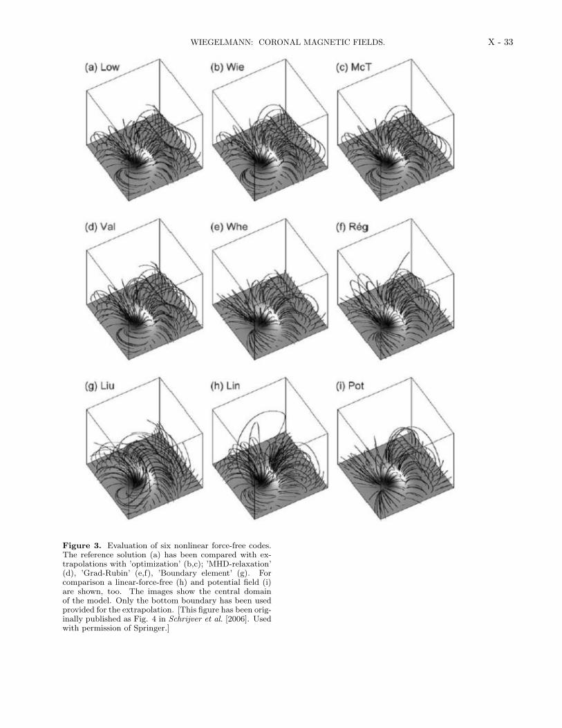
WIEGELMANN: CORONAL MAGNETIC FIELDS. X - 33
Figure 3. Evaluation of six nonlinear force-free codes.The reference solution (a) has been compared with ex-trapolations with ’optimization’ (b,c); ’MHD-relaxation’(d), ’Grad-Rubin’ (e,f), ’Boundary element’ (g). Forcomparison a linear-force-free (h) and potential field (i)are shown, too. The images show the central domainof the model. Only the bottom boundary has been usedprovided for the extrapolation. [This figure has been orig-inally published as Fig. 4 in Schrijver et al. [2006]. Usedwith permission of Springer.]