Embed Size (px)
Citation preview

Nonlinear Economic Model Predictive Control forEnergy Management of Smart Buildings
Rui Filipe Mirra dos Santos
Thesis to obtain the Master of Science Degree in
Mechanical Engineering
Supervisors: Prof. João Miguel da Costa SousaProf. Luís Manuel Fernandes Mendonça
Dr. Yi Zong
Examination CommitteeChairperson: Prof. João Rogério Caldas PintoSupervisor: Prof. João Miguel da Costa Sousa
Member of the Committee: Prof. Mário Manuel Gonçalves da Costa
October 2016

Instituto Superior TécnicoInstitute of Mechanical Engineering (IDMEC)Av. Rovisco Pais, 1, 1049-001 Lisboa, PortugalPhone +351 [email protected]://www.idmec.ist.utl.pt

Acknowledgments
First and foremost, I would like to express my sincere gratitude to my three supervisors, Prof. JoãoM. C. Sousa, Prof. Luís Mendonça and Dr. Yi Zong, for their unconditional support and cooperationthroughout the thesis period. Their guidance and knowledge was absolutely determinant for the successof the developed work.
Besides my supervisors, I’m extremely grateful to Dr. Shi You, for sharing with me his deep knowledgeof Power Systems, Dr. Anders Thavlov, for discussing key issues regarding the modeling phase of thiswork, Daniel Arndtzen, for giving me the technical support regarding sensor and actuator informationand heat pump specifications and Anders Bro Pedersen, for helping me with the SYSLAB database anddata acquisition.
My sincere thanks also goes to Eva Bülow Nielsen and Helle Faber, for their help, during the period Iwas in Denmark, regarding administrative issues, and to my two colleagues, Pedro Guimarães and HarisZiras, who never denied me their help, during the course of this work.
Finally, I would like to express my profound gratitude to my family and friends that, each in their ownway, were crucial during the course of my studies, believed in me and supported me in every way theycould. This accomplishment would not have been possible without all of them. Thank you.
i

Summary
Nowadays, buildings represent over one-third of the world-wide final energy consumption, in which 60%and 43% are used for heating purposes, in cold climate countries and warm climate countries, respectively.Therefore, the huge energetic impact they have, together with the high thermal inertia as a buildingfeature, makes them play a crucial role in the so called Demand Response (DR), which aims to useadaptive consumption to meet instantaneous generation. To do so, due to the complexity, nonlinearityand uncertainty in the energy systems, there is a need for developing intelligent control techniques capableof managing the full energy portfolio. In this thesis two different models, for the heat dynamics of aresidential building, a Stochastic Differential Equation (SDE) state-space model and a Takagi- Sugeno(TS) fuzzy model, both based on real-time measurement data, were developed. A new version of EconomicModel Predictive Control (EMPC), that uses the branch-and-bound optimization method, was capableof operating based on a nonlinear model, with a performance that was improved by the integration ofa fuzzy predictive filter. To show the controller capabilities on performing centralized control of multi-energy systems, a heat pump with a hot water tank storage was modeled and integrated in the system.The simulation results show that centralizing the temperature control of the building with the relatedresidential heat pump and its storage units brings up significant advantages. In fact, the operationcost reduced to about 16% and energy consumption to about 25%, while maintaining the comfort andenvironmental quality.
Keywords: Economic Model Predictive Control, nonlinear modeling, fuzzy modeling, fuzzy predic-tive filter, multi-energy systems, building energy management systems
iii


Resumo
Nos dias de hoje, os edifícios representam mais de um terço do consumo mundial final de energia, sendoque 60% é usado em aquecimento, em países de clima frio, e 43%, em países de clima quente. Conse-quentemente, o seu grande impacto energético, juntamente com a característica e elevada inércia térmica,fá-los desempenhar um papel crucial no chamado Demand Response (DR), que tem como objectivo usar oconsumo adaptativo para equilibrar a potência gerada. Para tal, devido à complexidade, não-linearidadee incerteza abundantes nos sistemas de energia, existe a necessidade de desenvolver técnicas de controlointeligente, capazes de gerir o portefólio energético. Neste trabalho são desenvolvidos dois modelos paradinâmica térmica de um edifício residencial, baseados em dados reais: um modelo em espaço de estados,baseado em Equações Diferenciais Estocásticas (SDE), e um modelo fuzzy do tipo Takagi-Sugeno (TS).Com recurso ao método de optimização branch-and-bound, o controlador mostrou-se capaz de operar osistema, baseando-se num modelo não-linear, com uma performance que foi melhorada pela integração deum filtro preditivo fuzzy. Para mostrar as capacidades do controlador na realização de controlo central-izado de sistemas multi-energéticos, modelou-se e integrou-se uma bomba de calor com armazenamentode água quente. A simulação realizada demonstra que centralizar o controlo de um edifício com a respec-tiva bomba de calor residencial e o armazenamento associado, traz vantagens significativas. Constatou-seainda que, o custo de operação foi reduzido para cerca de 16% e o consumo energético para cerca de 25%,mantendo-se o conforto e qualidade ambiental.
Palavras-chave: Economic Model Predictive Control, modelação não-linear, modelação fuzzy,filtro preditivo fuzzy, sistemas multi-energéticos, sistemas de gestão de energia em edifícios
v


Nomenclature
Clustering and Fuzzy Theory
K Number of fuzzy rules
Ri ith fuzzy rule
βi Fulfillment of the antecedent of the ith rule
N Cardinality of the data set
R Covariance matrix of the output
Bij Membership function for the ith rule and the jth state
ai Slope for the ith consequent
bi Constant for the ith consequent
µBi Membership grade of the ith rule antecedent
c Number of clusters
m Fuzziness parameter
µik Entry (i, k) of the partition matrix
vi Cluster center i
zk Data point k
Fi Cluster covariance matrix of the ith cluster
λin Smallest eigenvalue of the cluster covariance matrix
λi1 Largest eigenvalue of the cluster covariance matrix
γik Normalized membership degree of the kth diagonal entry
µec Electricity cost membership grade
vii

Control and Systems Theory
ts Sampling time
ωn Cutoff frequency
ωs Sampling frequency
τc Time-lag
τy First local minimum of the linear correlation function
τy2′ First local minimum of the nonlinear correlation function
τm Faster local minimum of both linear and nonlinear correlation functions
x State vector
u Input vector
y Output vector
y Estimated output vector
θ Parameter vector
θ Estimated parameter vector
t Time variable
k Discrete time variable
σ Diffusion term of the stochastic process
ω Standard Wiener process
e White noise process
fSDE Stochastic differential equation drift term
hSDE Stochastic differential equation measurement function
X Data point state matrix
Xe Extended regressor matrix
εp One-step ahead prediction error
Θ Parameters search space, for the maximum likelihood estimation problem
A Jacobian of the stochastic differential equations model
x Estimated state
˙x Estimated state derivative
P Covariance matrix of the state
C Output matrix of the state-space model
umin Minimum control action vector
viii

umax Maximum control action vector
u∗ Optimal control action vector
∆u Change in the control action vector
∆umin Minimum change in the control action vector
∆umax Maximum change in the control action vector
u+k Positive change in the control action
u−k Negative change in the control action
r Reference vector
ymin Minimum output vector
ymax Maximum output vector
d Disturbance vector
d Estimated disturbance vector
Heat Transfer and Thermodynamics Theory
q′′cond Conductive heat flux vector per unit of area
kcond Thermal conductivity
T Scalar temperature field
ρm Density of the material
cp Specific heat capacity
qg Rate of thermal energy generation within the medium
A Area of the wall normal to the direction of heat transfer
qcondx Conductive heat transfer rate in the x direction
L Thickness of the wall
Ts,i Inside wall surface temperature
Ts,o Outside wall surface temperature
U Overall heat transfer coefficient
Nwl Number of wall layers
∆T Temperature difference between the inside and outside wall surfaces
q′′conv Convective heat transfer rate per unit of area
hconv Convective heat transfer coefficient
Tsur Surface temperature
ix

Trad Surroundings radiant temperature
T∞ Fluid temperature
q′′rad Radiation heat transfer rate per unit of area
ε Emissivity
σSB Stefan-Boltzmann constant
h Specific enthalpy
Qin Heat transfer rate from the cold source of the heat pump
Qout Heat transfer rate to the warm source of the heat pump
Wc Compressor power input rate
Wmaxc Maximum compressor power input rate
m Mass flow rate
Mathematics
σ0 Standard deviation vector
ρp Pearson’s Correlation
Ryy Linear correlation function
Ry2′y2′ Nonlinear correlation function
f Probability density function
ly Dimension of the output vector
L Conditional likelihood function
l log-likelihood function
Clh Constant term in the likelihood function
Model Predictive Control – Optimization
Np Prediction horizon
Nc Control horizon
w1 Weight in the objective function, associated with the reference tracking
w2 Weight in the objective function, associated with the change in the control action
J Objective function cost for the traditional Model Predictive Control
JE Objective function cost for the Economic Model Predictive Control
x

nd Number of control alternatives for each input
Ω Control space
µi ith control alternative
J(j)i Cost associated with a transition, from the discrete time step j to the discrete time step j + 1,
by means of applying the control action µi
J(j)c,i Cumulative cost function associated with a transition, from the discrete time step j to the
discrete time step j + 1, by means of applying the control action µi
vk Slack variables vector
ρv Penalty cost associated with the slack variable vk
∆Ω Adaptive set of control action change alternatives
η Scaling factor in the fuzzy predictive filter
Nf Dimension index for the control space cardinality, using fuzzy predictive filter
λl Control alternatives’ space distribution function
Smart Buildings Modeling
ΦS Solar irradiation power
Tb Basement temperature
Tf1 First-floor temperature
Tf2 Second-floor temperature
Teb Basement envelope temperature
Te1 First-floor envelope temperature
Te2 Second-floor envelope temperature
Ta Ambient temperature
Wspd Wind speed
Wdir Wind direction
Φair Heat power due to convection with the ambient air
Φearth Heat power through the earth/basement interface
Φbf Heat power through the basement/first-floor interface
Φff Heat power through the first-floor/second-floor interface
ΦHb Radiator power input in the basement
ΦH1 Radiator power input in the first-floor
xi

ΦH2 Radiator power input in the second-floor
σb Diffusion term for the stochastic process associated with the basement state
σeb Diffusion term for the stochastic process associated with the basement envelope state
σf1 Diffusion term for the stochastic process associated with the first-floor state
σe1 Diffusion term for the stochastic process associated with the first-floor envelope state
σf2 Diffusion term for the stochastic process associated with the second-floor state
σe2 Diffusion term for the stochastic process associated with the second-floor envelope state
ωb Wiener process associated with the basement state
ωeb Wiener process associated with the basement envelope state
ωf1 Wiener process associated with the first-floor state
ωe1 Wiener process associated with the first-floor envelope state
ωf2 Wiener process associated with the second-floor state
ωe2 Wiener process associated with the second-floor envelope state
ub Radiator control action in the basement floor
u1 Radiator control action in the first-floor floor
u2 Radiator control action in the second-floor floor
ΦHi Radiator power input in the ith floor
ΦmaxHi Maximum radiator power input in the ith floor
ΦmaxHb Maximum radiator power input in the basement floor
ΦmaxH1 Maximum radiator power input in the first-floor floor
ΦmaxH2 Maximum radiator power input in the second-floor floor
Re1a Thermal resistance between the first-floor envelope and the ambient
Re2a Thermal resistance between the second-floor envelope and the ambient
cW Multiplicative term in the nonlinear relation of the convective resistance
γW Exponent term in the general nonlinear relation of the convective resistance
cW1 Multiplicative term in the nonlinear relation of the convective resistance, for the first-floor
γW1 Exponent term in the nonlinear relation of the convective resistance, for the first-floor
cW2 Multiplicative term in the nonlinear relation of the convective resistance, for the second-floor
γW2 Exponent term in the nonlinear relation of the convective resistance, for the second-floor
θ0 Angle offset related to the building orientation
Tearth Earth temperature
xii

Awb Effective window area of the basement
Aw1 Effective window area of the first-floor
Aw2 Effective window area of the second-floor
Cb Heat capacity of the basement
Cf1 Heat capacity of the first-floor
Cf2 Heat capacity of the second-floor
Ceb Heat capacity of the basement envelope
Ce1 Heat capacity of the first-floor envelope
Ce2 Heat capacity of the second-floor envelope
Rff Thermal resistance between the first-floor and the second floor
Rfb Thermal resistance between the first-floor and the basement
Reeb Thermal resistance between the earth surroundings and the basement envelope
Rbeb Thermal resistance between the basement and the basement envelope
Rf1e1 Thermal resistance between the first-floor and the first-floor envelope
Rf2e2 Thermal resistance between the second-floor and the second-floor envelope
c Price signal vector
Ψ Comfort index function
Tsupply Supply water temperature (assumed to be constant)
Tw Stored water temperature
Cw Heat capacity of the water tank
cp Water specific heat
ρw Water density
Atank Surface area of the considered water tank
qmax Maximum volumetric water flow rate in each floor
QHP Heat transfer rate provided by the heat pump
Qloss Losses to the environment
qT Total volumetric water flow supplied to the building
Rwtb Thermal resistance between the water and the basement air
Rih Thermal resistance between a certain radiator and the respective floor i
Ti Indoor temperature in the ith floor
Rbh Thermal resistance between the basement radiator and the basement floor
Rf1h Thermal resistance between the first-floor radiator and the first-floor
Rf2h Thermal resistance between the second-floor radiator and the second-floor
xiii


Acronyms
Clustering and Fuzzy Theory
ACF Average Cluster Flatness
APD Average Partition Density
AWCD Average Within-Cluster Distance
FHV Fuzzy Hypervolume
MF Membership Functions
TS Takagi-Sugeno
Control and Systems Theory
ARE Algebraic Riccati Equation
EKF Extended Kalman Filter
EMPC Economic MPC
LQG Linear Quadratic Gaussian
LQR Linear Quadratic Regulator
MBPC Model Based Predictive Control
MIMO Multiple-Input Multiple-Output
MPC Model Predictive Control
NMPC Nonlinear MPC
PID Proportional Integrative Derivative
xv

Mathematics
CDF Cumulative Distribution Function
MAE Mean Absolute Error
MLE Maximum Likelihood Estimator
MSE Mean Squared Error
NLSDE Nonlinear Stochastic Differential Equations
ODE Ordinary Differential Equations
PRBS Pseudo Random Binary Sequence
RMSE Root Mean Squared Error
SDE Stochastic Differential Equations
VAF Variance Accounted For
Smart Grid and Smart Buildings
BEMS Building Energy Management Systems
COP Coefficient of Performance
CHP Combined Heat and Power
DER Distributed Energy Resources
DR Demand Response
PMV Predicted Mean Vote
RC Resistor-Capacitor
Other
CFD Computational Fluid Dynamics
CRISP-DM CRoss Industry Standard Process for Data Mining
CTSM-R Continuous Time Stochastic Modeling for R
DTU Technical University of Denmark
OECD Organisation for Economic Co-operation and Development
SQP Sequential Quadratic Programming
xvi

xvii


Contents
Acknowledgments i
Summary iii
Resumo v
Nomenclature vii
Acronyms xv
List of Tables xxi
List of Figures xxiii
1 Introduction 11.1 Motivation for Building Energy Management Systems . . . . . . . . . . . . . . . . . . . . 1
1.1.1 The Future Energy System . . . . . . . . . . . . . . . . . . . . . . . . . . . . . . . 11.1.2 Nonlinear Economic Model Predictive Control . . . . . . . . . . . . . . . . . . . . 4
1.2 Contributions . . . . . . . . . . . . . . . . . . . . . . . . . . . . . . . . . . . . . . . . . . . 51.3 Outline . . . . . . . . . . . . . . . . . . . . . . . . . . . . . . . . . . . . . . . . . . . . . . 6
2 Data Analysis for Smart Buildings 92.1 Intelligent Data Analysis . . . . . . . . . . . . . . . . . . . . . . . . . . . . . . . . . . . . . 92.2 Project and Data Understanding . . . . . . . . . . . . . . . . . . . . . . . . . . . . . . . . 102.3 Data Preprocessing . . . . . . . . . . . . . . . . . . . . . . . . . . . . . . . . . . . . . . . . 12
2.3.1 Measurement Data . . . . . . . . . . . . . . . . . . . . . . . . . . . . . . . . . . . . 122.3.2 Experimental Data . . . . . . . . . . . . . . . . . . . . . . . . . . . . . . . . . . . . 172.3.3 Forecast Data . . . . . . . . . . . . . . . . . . . . . . . . . . . . . . . . . . . . . . . 17
2.4 The Sampling Time . . . . . . . . . . . . . . . . . . . . . . . . . . . . . . . . . . . . . . . 21
3 Modeling 233.1 Heat Transfer Phenomena . . . . . . . . . . . . . . . . . . . . . . . . . . . . . . . . . . . . 23
3.1.1 Conduction . . . . . . . . . . . . . . . . . . . . . . . . . . . . . . . . . . . . . . . . 233.1.2 Convection . . . . . . . . . . . . . . . . . . . . . . . . . . . . . . . . . . . . . . . . 253.1.3 Radiation . . . . . . . . . . . . . . . . . . . . . . . . . . . . . . . . . . . . . . . . . 25
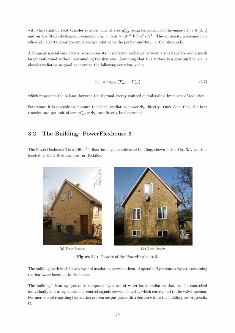
3.2 The Building: PowerFlexhouse 3 . . . . . . . . . . . . . . . . . . . . . . . . . . . . . . . . 263.3 Stochastic Differential Equations State-Space Model . . . . . . . . . . . . . . . . . . . . . 28
3.3.1 Parameter Estimation – Maximum Likelihood Estimator . . . . . . . . . . . . . . . 303.3.2 Extended Kalman Filter . . . . . . . . . . . . . . . . . . . . . . . . . . . . . . . . . 343.3.3 Model Validation . . . . . . . . . . . . . . . . . . . . . . . . . . . . . . . . . . . . . 34
3.4 Takagi-Sugeno Fuzzy Model . . . . . . . . . . . . . . . . . . . . . . . . . . . . . . . . . . . 353.4.1 Sensitivity Analysis – Number of Clusters . . . . . . . . . . . . . . . . . . . . . . . 373.4.2 Parameter Estimation – Global Least-squares Method . . . . . . . . . . . . . . . . 393.4.3 Model Generation and Simplification . . . . . . . . . . . . . . . . . . . . . . . . . . 41
xix
3.4.4 Model Validation . . . . . . . . . . . . . . . . . . . . . . . . . . . . . . . . . . . . . 453.5 Discussion . . . . . . . . . . . . . . . . . . . . . . . . . . . . . . . . . . . . . . . . . . . . . 46
4 Economic Model Predictive Control 474.1 MPC Overview . . . . . . . . . . . . . . . . . . . . . . . . . . . . . . . . . . . . . . . . . . 474.2 MPC General Formulation . . . . . . . . . . . . . . . . . . . . . . . . . . . . . . . . . . . . 484.3 EMPC Formulation . . . . . . . . . . . . . . . . . . . . . . . . . . . . . . . . . . . . . . . 494.4 EMPC Design . . . . . . . . . . . . . . . . . . . . . . . . . . . . . . . . . . . . . . . . . . . 51
4.4.1 The Optimization Algorithm . . . . . . . . . . . . . . . . . . . . . . . . . . . . . . 514.4.2 Ensuring the Feasibility under Uncertain Scenarios: Soft-Constraints . . . . . . . . 554.4.3 Fuzzy Predictive Filters . . . . . . . . . . . . . . . . . . . . . . . . . . . . . . . . . 58
4.5 Discussion . . . . . . . . . . . . . . . . . . . . . . . . . . . . . . . . . . . . . . . . . . . . . 62
5 Coupling Electricity and Heating via Heat Pump Integration 635.1 Multi-Energy Systems Overview . . . . . . . . . . . . . . . . . . . . . . . . . . . . . . . . 635.2 Heat Pump Modeling . . . . . . . . . . . . . . . . . . . . . . . . . . . . . . . . . . . . . . 645.3 Water Tank Modeling . . . . . . . . . . . . . . . . . . . . . . . . . . . . . . . . . . . . . . 655.4 System Integration . . . . . . . . . . . . . . . . . . . . . . . . . . . . . . . . . . . . . . . . 665.5 Energetic Assessment . . . . . . . . . . . . . . . . . . . . . . . . . . . . . . . . . . . . . . 675.6 Discussion . . . . . . . . . . . . . . . . . . . . . . . . . . . . . . . . . . . . . . . . . . . . . 69
6 Conclusions 71
Bibliography 75
Appendices 81
A Data Summary 81
B Sensor and Actuator Location 83
C PowerFlexhouse 3: Heating Power Distribution 87
D Extended Kalman Filter – Matrices 89
E Model Validation – Plots 91E.1 SDE State Space Model . . . . . . . . . . . . . . . . . . . . . . . . . . . . . . . . . . . . . 92E.2 TS Fuzzy Model . . . . . . . . . . . . . . . . . . . . . . . . . . . . . . . . . . . . . . . . . 95
F Branch-and-bound algorithm for EMPC 99
G Heat Pump Specifications 101
H Water Tank Specifications 103
xx

List of Tables
Introduction 1
Data Analysis for Smart Buildings 9
2.1 Forecast performance measures for the weather conditions. . . . . . . . . . . . . . . . . . . 21
2.2 Autocorrelation faster local minimums τm, in minutes, for each data set and for each output. 22
Modeling 23
3.1 Thermal dynamics variables description. . . . . . . . . . . . . . . . . . . . . . . . . . . . . 27
3.2 Estimated model parameters for the system. . . . . . . . . . . . . . . . . . . . . . . . . . . 32
3.3 Performance assessment of the Stochastic Differential Equations state-space model for the4-season simulation. . . . . . . . . . . . . . . . . . . . . . . . . . . . . . . . . . . . . . . . 36
3.4 Number of clusters results, applying the cluster validity measures. . . . . . . . . . . . . . 38
3.5 Statistic properties regarding the validation of the 30 Takagi-Sugeno fuzzy models generated. 42
3.6 Takagi-Sugeno fuzzy model of the PowerFlexhouse 3. . . . . . . . . . . . . . . . . . . . . . 44
3.7 Performance assessment of the Takagi-Sugeno fuzzy model of the 4-season simulation. . . 46
Economic Model Predictive Control 47
4.1 Traditional Model Predictive Control vs Economic Model Predictive Control. . . . . . . . 51
4.2 Performance assessment of the Economic Model Predictive Control, in a 5-day simulationscenario, using hard-constraints. . . . . . . . . . . . . . . . . . . . . . . . . . . . . . . . . 55
xxi

4.3 Performance assessment of the Economic Model Predictive Control, in a 5-day simulationscenario, using soft-constraints and fuzzy predictive filtering. . . . . . . . . . . . . . . . . 61
Coupling Electricity and Heating via Heat Pump Integration 63
5.1 Model parameters for the hot water tank model. . . . . . . . . . . . . . . . . . . . . . . . 66
5.2 Performance comparison, with and without heat pump system, using the Economic ModelPredictive Control, in a 5-day simulation scenario. . . . . . . . . . . . . . . . . . . . . . . 68
Conclusions 71
Appendices 81
A.1 Description of each data type in the considered data set. . . . . . . . . . . . . . . . . . . . 82
C.1 Maximum heat power (kW) distribution among each floor, together with total equivalentpower. . . . . . . . . . . . . . . . . . . . . . . . . . . . . . . . . . . . . . . . . . . . . . . . 87
xxii

List of Figures
Introduction 1
1.1 Final world energy consumption from 1971 to 2013 by fuel. . . . . . . . . . . . . . . . . . 1
1.2 Total final electricity consumption from 1971 to 2013 by sector. . . . . . . . . . . . . . . . 2
1.3 Renewable power generation, by solar and wind generators, and power demand during aday. . . . . . . . . . . . . . . . . . . . . . . . . . . . . . . . . . . . . . . . . . . . . . . . . 2
1.4 Integrated and intelligent energy network of the future. . . . . . . . . . . . . . . . . . . . 3
1.5 Final world energy consumption by sector and buildings energy mix. . . . . . . . . . . . . 3
1.6 Buildings end-use energy consumption. . . . . . . . . . . . . . . . . . . . . . . . . . . . . . 4
1.7 Timeline of the computation power evolution. . . . . . . . . . . . . . . . . . . . . . . . . . 5
Data Analysis for Smart Buildings 9
2.1 Overview of the CRoss Industry Standard Process for Data Mining process. . . . . . . . . 10
2.2 Data-flow through a black-box representative model. . . . . . . . . . . . . . . . . . . . . . 10
2.3 Trends of the relevant data types during the day of 1 JAN 2015. . . . . . . . . . . . . . . 11
2.4 Daily time series of the ambient temperature data, measured each second, for the fourseasons. . . . . . . . . . . . . . . . . . . . . . . . . . . . . . . . . . . . . . . . . . . . . . . 13
2.5 Daily time series of the wind speed data, measured each second, for the four seasons. . . . 14
2.6 Daily time series of the wind direction data, measured each second, for the four seasons. . 15
2.7 Daily time series of the solar irradiation data, measured each second, for the four seasons. 16
xxiii

2.8 Data collected during the Pseudo Random Binary Sequence experiment. . . . . . . . . . . 18
2.9 Mean weather forecasts and mean observations in each month. . . . . . . . . . . . . . . . 19
2.10 Scatterplot of observed measurements against respective forecasts. . . . . . . . . . . . . . 20
Modeling 23
3.1 Facades of the PowerFlexhouse 3. . . . . . . . . . . . . . . . . . . . . . . . . . . . . . . . . 26
3.2 Sketch of the thermal dynamics through the building. . . . . . . . . . . . . . . . . . . . . 27
3.3 Resistor-Capacitor equivalent circuit diagram for the PowerFlexhouse 3. . . . . . . . . . . 29
3.4 Nonlinear convection resistances, function of wind speed and wind direction. . . . . . . . . 33
3.5 Stochastic Differential Equations state-space model simulation, without Extended KalmanFilter, performed during 96 spring hours starting from 8 APR 2013. . . . . . . . . . . . . 33
3.6 Stochastic Differential Equations state-space model simulation, with Extended KalmanFilter, performed during 30 winter days, starting from 1 DEC 2014. . . . . . . . . . . . . 35
3.7 Takagi-Sugeno fuzzy inference system. . . . . . . . . . . . . . . . . . . . . . . . . . . . . . 36
3.8 Cluster validity measures. . . . . . . . . . . . . . . . . . . . . . . . . . . . . . . . . . . . . 39
3.9 Fuzzy sets used in the Takagi-Sugeno fuzzy model. . . . . . . . . . . . . . . . . . . . . . . 43
3.10 Takagi-Sugeno fuzzy model simulation performed during 30 winter days, starting from 1DEC 2014. . . . . . . . . . . . . . . . . . . . . . . . . . . . . . . . . . . . . . . . . . . . . 45
Economic Model Predictive Control 47
4.1 Model Predictive Control basic principle. . . . . . . . . . . . . . . . . . . . . . . . . . . . 48
4.2 Model Predictive Control general algorithm. . . . . . . . . . . . . . . . . . . . . . . . . . . 49
4.3 Supply curve shifting and its reflection in the price. . . . . . . . . . . . . . . . . . . . . . . 50
4.4 Hourly electricity spot price and wind power penetration during JAN 2015. . . . . . . . . 50
4.5 Economic Model Predictive Control block diagram scheme. . . . . . . . . . . . . . . . . . 52
4.6 Branch-and-bound search tree for model predictive control applications. . . . . . . . . . . 52
4.7 Example of control space discretization. . . . . . . . . . . . . . . . . . . . . . . . . . . . . 53
xxiv
4.8 Simulation performed during five days starting from 1 JAN 2015, using the hard-constraintsEconomic Model Predictive Control formulation. . . . . . . . . . . . . . . . . . . . . . . . 54
4.9 Time series of the weather disturbances designed for feasibility studies. . . . . . . . . . . . 56
4.10 Simulation performed during five days starting from 1 JAN 2015, using the hard-constraintsEconomic Model Predictive Control formulation, with the additional weather disturbancesillustrated in Figure 4.9. . . . . . . . . . . . . . . . . . . . . . . . . . . . . . . . . . . . . . 56
4.11 Simulation performed during five days starting from 1 JAN 2015, using the soft-constraintsEconomic Model Predictive Control formulation, with the additional weather disturbancesillustrated in Figure 4.9. . . . . . . . . . . . . . . . . . . . . . . . . . . . . . . . . . . . . . 58
4.12 General adaptive Membership Function for the Electricity Price. . . . . . . . . . . . . . . 59
4.13 Economic Model Predictive Control scheme with fuzzy predictive filtering. . . . . . . . . . 60
4.14 Simulation performed during five days starting from 1 JAN 2015, using the soft-constraintsEconomic Model Predictive Control formulation and fuzzy predictive filtering. . . . . . . . 60
4.15 Computation time distribution for all the control decisions made by the Economic ModelPredictive Control, using soft-constraints and fuzzy predictive filtering in a 5-day simulation. 61
Coupling Electricity and Heating via Heat Pump Integration 63
5.1 Heap pump thermodynamic cycle. . . . . . . . . . . . . . . . . . . . . . . . . . . . . . . . 64
5.2 Water tank thermal dynamics scheme. . . . . . . . . . . . . . . . . . . . . . . . . . . . . . 65
5.3 Simulation performed during five days starting from 1 JAN 2015, controlling the buildingtemperature with integrated heat pump and hot water tank, using the soft-constraintsEconomic Model Predictive Control formulation and no fuzzy predictive filter. . . . . . . . 68
Conclusions 71
Appendices 81
E.1 Stochastic Differential Equations State Space Model simulation, with Extended KalmanFilter performed during 30 autumn days, starting from 11 OCT 2014. . . . . . . . . . . . 92
E.2 Stochastic Differential Equations State Space Model simulation, with Extended KalmanFilter performed during 30 spring days, starting from 1 MAY 2015. . . . . . . . . . . . . . 93
E.3 Stochastic Differential Equations State Space Model simulation, with Extended KalmanFilter, performed during 30 summer days, starting from 7 JUL 2014. . . . . . . . . . . . . 94
xxv

E.4 Takagi-Sugeno fuzzy model simulation performed during 30 autumn days, starting from11 OCT 2014. . . . . . . . . . . . . . . . . . . . . . . . . . . . . . . . . . . . . . . . . . . . 95
E.5 Takagi-Sugeno fuzzy model simulation performed during 30 spring days, starting from 1MAY 2015. . . . . . . . . . . . . . . . . . . . . . . . . . . . . . . . . . . . . . . . . . . . . 96
E.6 Takagi-Sugeno fuzzy model simulation performed during 30 summer days, starting from 7JUL 2014. . . . . . . . . . . . . . . . . . . . . . . . . . . . . . . . . . . . . . . . . . . . . . 97
xxvi

Chapter 1
Introduction
1.1 Motivation for Building Energy Management Systems
1.1.1 The Future Energy System
For the last centuries, energy was responsible for a tremendous amount of changes in our planet. Nowadaysit is not only a key factor in the modern civilization, but also the biggest “fuel” for continuous development,being highly correlated with it. However, the abusive consumption of fossil fuels has triggered a set ofundesirable events, such as the climate change, that are risking the sustainable development. This isperhaps one of the biggest challenges the human society has been facing, motivating several internationalcommitments and collaborations, such as the Organisation for Economic Co-operation and Development(OECD) example.
The energy requirements are illustrated, among the years, in Figure 1.1. It shows an increasing trend,meaning that the right decisions have to be made in order to decrease the share of fossil fuels-basedenergy generation and increase the share of renewable-based energy generation.
28
CONSUMPTION
28
CONSUMPTION
TOTAL FINAL CONSUMPTION
World
Other4Natural gas
Biofuels and waste3
Coal2
Electricity
Oil
0
2 000
4 000
6 000
8 000
10 000
1971 1975 1980 1985 1990 1995 2000 2005 2010 2013
1 total final consumption from 1971 to 2013 by fuel (Mtoe)
1973 and 2013 fuel shares of total final consumption
1. World includes international aviation and international marine bunkers.2. In these graphs, peat and oil shale are aggregated with coal.
3. Data for biofuels and waste final consumption have been estimated for a number of countries.4. Includes geothermal, solar, wind, heat, etc.
1973 2013
Coal²13.6%
Oil48.3%Natural gas
14.0%
Biofuels andwaste³
13.1%
Electricity9.4%
Other41.6%
Biofuels andwaste³
12.2%
Electricity18.0%
Other4
3.3%Coal²11.5%
Oil39.9%
Natural gas15.1%
4 667 Mtoe 9 301 Mtoe
© O
ECD
/IEA
, 20
15
World
Figure 1.1: Final world energy consumption from 1971 to 2013 by fuel (source [24]).
1
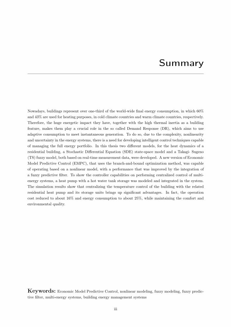
Motivated by the environmental problems that have been verified, a phenomenon called electrification hasemerged, which consists in increasing the share of electricity consumption within the total world energyconsumption, as can be confirmed while analyzing the trend presented in Figure 1.2. With this change,it is possible to base the electricity generation upon renewable generators and, consequently, increase theshare of renewable energy sources in the total world energy consumption.
3
35
Electricity
Other1TransportIndustry
0
200
400
600
800
1 000
1 200
1 400
1 600
1 800
1971 1975 1980 1985 1990 1995 2000 2005 2010 2013
Total final consumption from 1971 to 2013 by sector (Mtoe)
1973 and 2013 shares of world electricity consumption
440 Mtoe 1 677 Mtoe
1. Includes agriculture, commercial and public services, residential, and non-specified other.
1973 2013
Industry53.4%
Transport2.4%
Other144.2% Other1
56.2%
Industry42.3%
Transport1.5%
BY SECTOR©
OEC
D/I
EA, 2
01
5
Figure 1.2: Total final electricity consumption from 1971 to 2013 by sector (source [24]).
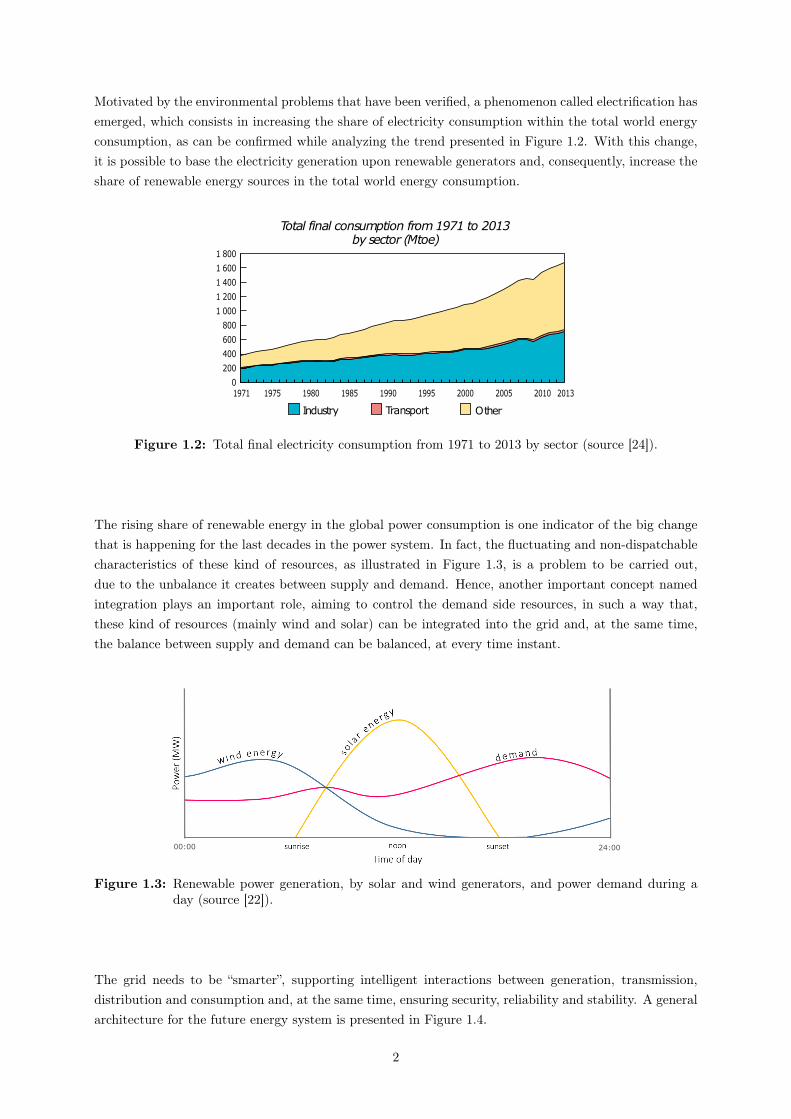
The rising share of renewable energy in the global power consumption is one indicator of the big changethat is happening for the last decades in the power system. In fact, the fluctuating and non-dispatchablecharacteristics of these kind of resources, as illustrated in Figure 1.3, is a problem to be carried out,due to the unbalance it creates between supply and demand. Hence, another important concept namedintegration plays an important role, aiming to control the demand side resources, in such a way that,these kind of resources (mainly wind and solar) can be integrated into the grid and, at the same time,the balance between supply and demand can be balanced, at every time instant.
Energy Storage - Hydrogenious TechnologiesHydrogenious Technologies http://www.hydrogenious.net/en/energy-storage/
1 de 6 11-06-2016 16:41
00:00 24:00
Figure 1.3: Renewable power generation, by solar and wind generators, and power demand during aday (source [22]).
The grid needs to be “smarter”, supporting intelligent interactions between generation, transmission,distribution and consumption and, at the same time, ensuring security, reliability and stability. A generalarchitecture for the future energy system is presented in Figure 1.4.
2

Figure 1.4: Integrated and intelligent energy network of the future (source [23]).
To meet the desired goals and design the new smart grid, the development of new technologies, capableof addressing the mentioned challenges, is a key issue.
According to Figure 1.5, buildings are responsible for 35% of the world’s final energy consumption. Itis then a common interest to develop advanced and innovative intelligent control techniques that canmanage energy in those buildings.
Thispublicationispartof theIEAEnergyTechnologyPerspectives(ETP)seriesandfocusesonthekeybuildingtechnologiesandsystemsthatneedtobepromotedanddeployed,alongwithrecommendationsonresearchanddevelopment(R&D)toachievemajorreductionsinenergyconsumptionandCO2emissionsinthebuildingssectorthroughto2050.It isintendedformultipleaudiencesincludingpolicymakers,industry,researchers,efficiencyadvocates,investorsandpractitionerswithlimitedorextensivebackgroundsinthebuildingssector.It isalsointendedtoserveasareferencedocumentthataddressesmajortechnologiesthatneedtobepursuedinbothdevelopedanddevelopingcountries,alongwithsupportingpolicies.
Thebuildingssector,comprisingboththeresidentialandservicessub-sectors(Box1.1),consumes35%of global finalenergyuse(Figure1.1).It isresponsibleforabout17%of totaldirectenergy-relatedCO2emissionsfromfinalenergyconsumers.If indirectupstreamemissionsattributabletoelectricityandheatconsumptionaretakenintoaccount,thesectorcontributesaboutone-thirdof globalCO2emissions.
Figure1.1 Final energyconsumptionbysectorandbuildingsenergymix,2010
f:\2000\image\155992\\2
Notes:final energy consumption excludes non-energyuse.Other sectors include agriculture, forestry, fishing and other non-specified.Source:unless otherwise noted,all tables and figure in this chapter are derived fromIEA data and analysis.
Keypoint Buildingsareamajor end-useinglobal energymarketsandneedtobeastrongcomponentof anycountry’splantosaveenergy.
Thebuildingssectorusesawidearrayof technologies.Theyareusedinthebuildingenvelopeanditscomponents,inspaceheatingandcoolingsystems,inwaterheating,inlighting,inappliancesandconsumerproducts,andinofficeandserviceequipment.Therearenumerousmeasuresthatarealreadycosteffectiveandshouldbepursuedimmediately.Otherscanbecomecosteffectivewithmodestgovernmentsupportandincentives.Therearealsomanyareasthat,alongwithsynergiesandanintegratedsystemsapproach,will result inleast-costoptionsandthegreatestenergy-savingpotential.Theseshouldcertainlybepursued.
Duetothelonglifetimeof buildingsandrelatedequipment,combinedwithprevailingfinancialbarriersinthesector,manybuildingsdonotapplyexistingefficient technologiestothedegreethat life-cyclecostminimisationwarrants.Amongthebarriersthatexist toimprovingenergyefficiencyanddecarbonisingenergyusearehigherinitialcosts,lackof consumerawarenessof technologiesandtheirpotential,split incentivesandthefact that thetruecostsof CO2emissionsarenotreflectedinmarketprices.Overcomingthesebarrierswillneedacomprehensive,sequencedpolicypackage,totargetspecificbarrierswitheffectivepolicyresponsesandenforcementmeasures.
©OECD/IEA, 2013.
26 Part1ScenariosfortheBuildingsSector
Chapter1BuildingsOverview
Figure 1.5: Final world energy consumption by sector and buildings energy mix (source [23]).
From the percentage presented in Figure 1.5, as it is notable in Figure 1.6, buildings end-use energyaccounts for 60%, which is used for heating purposes, in cold climate countries, and 43%, which is used forcooling purposes in warm climate countries. Therefore, the huge energetic impact they have, together withthe high thermal inertia as a characteristic building feature, makes them play a crucial role in the so calledDemand Response (DR), which consists of endowing the grid with adaptive consumption capabilities,with respect to some prescribed conditions. DR is being used by electricity grid managers to makebuildings smart grid aware and increase the grid flexibility, facilitating the penetration of intermittentenergy resources in the power system [25].
3

Figure1.6 Buildingsend-useenergyconsumption,2010
f:\2000\image\155992\\7
Notes:EJ=exajoule.ColdclimatecountriescompriseOECDcountriesexcludingAustralia,Mexico,NewZealandandIsrael,andnon-OECDEuropeandEurasia.The statistical data for Israel are supplied byandunder the responsibilityof the relevant Israeli authorities.The use of suchdata by theOECDand/or theIEA is without prejudice to the status of the GolanHeights,East Jerusalemand Israeli settlements in theWest Bankunder the terms of international law.
Keypoint About70%of buildingsenergyconsumption isfor spaceheatingandappliancesincoldclimates,andforwater heatingandcookinginmoderateandwarmclimates.
Thispublicationdoesnotprovideanexhaustiveanalysisof theneedforbehaviouralchange.However,it isrecognisedthat tobesuccessful,policieswillneedtotakeintoconsiderationconsumerinterestandensurenon-financialbarriers,suchaslackof information,lackofconsumerawarenessorpublicacceptance,areaddressed.Althoughitdoesnotexplicitlyquantifytheroleof consumerbehaviour,it is implicitlytakenintoconsiderationinthedevelopmentof thebuildingsmodelassumptions.Forexample,it isassumedthat thenumberof householdscurrentlyrelyingontraditionalbiomasswilldecreasedramatically.Whilesomehouseholdscurrentlyusetraditionalbiomassbychoice,theanalysisassumesthatconsumerpreferencewill leadtoamoveawayfromthisformof energyforcooking.
Current statusof energyandemissionsin thebuildingssectorEnergyconsumptiontrendsintheresidentialsub-sectorarecloselyrelatedtoawiderangeoffactors,includingchangesinpopulation,numberof households,buildingcharacteristics,buildingageprofile,housesize,incomegrowth,consumerpreferencesandbehaviour,climaticconditions,applianceownershiplevels,andoverallenergyefficiencyimprovements.Between1990and2010,theworld’spopulationgrewby30%toreach7.0billion.Mostof thisgrowthoccurredinnon-OECDcountries(Table1.1).
Intheservicessub-sector,energyconsumptiontrendsaremorecloselyrelatedtothesector’slevelof economicactivityandtherelatedgrowthinfloorarea,buildingtypes(relativetosectoractivity),ageof buildings,climaticconditionsandenergyefficiencyimprovements.Grossdomesticproduct(GDP)hasincreasedrapidly,almostdoublingbetween1990and2010.Theincreaseinthesector’svalue-added3wasevenfaster,globallyincreasingby3.3%peryear.
3 Value-addedcanbemeasuredeithergross ornet,that is,beforeorafter deducting consumptionof fixedcapital:a)grossvalue-added is the value of output less the value of intermediate consumption;and b) net value-added is the value ofoutput less the values of both intermediate consumption and consumption of fixed capital.
©OECD/IEA, 2013.
Part1ScenariosfortheBuildingsSector
Chapter1BuildingsOverview 31
Figure 1.6: Buildings end-use energy consumption (source [23]).
1.1.2 Nonlinear Economic Model Predictive Control
All the arguments presented in Section 1.1.1 justify the research that is being done, among the past fewdecades, related to intelligent control of energy use in smart buildings. Therefore, if equipped with theright control tools, the previously mentioned DR, is a concept that can take advantage of the buildings’large DR potential, coming from their natural thermal storage capacity.
Numerous varieties of Model Predictive Control (MPC) [33, 45] solutions have been successfully appliedto the referred problem. Specifically, the Economic MPC (EMPC) [60] and its ability of shifting theload away from the peak hours, lowering the cost of operation, makes it the most promising controltechnique within the new energy paradigm. Furthermore, the overlap of the large share of renewable-based electricity generation periods with the low electricity price periods, also guarantee an enhancementof renewable energy-based consumption.
Previous studies, such as [15, 64], applied linear EMPC strategies that were shown to be very effectiveto shape the behavior of the related energy systems, by making them smart.
Recently, it is notable an increase in a common effort, within the research community, on developing moreaccurate models for the energy systems. Unwittingly, this type of work ends up with a conclusion thatlinear models are not enough to describe the system dynamics needed for a specific application, if thenonlinearities are very determinant in the system behavior. Two examples are presented in [26], where itis proven that a linear model is not enough to describe a photovoltaic module dynamics and a nonlinearmodel is proposed and validated, and [9], that discusses the advantages of introducing nonlinear effectsrelated to the convection and radiation throughout the building.
With the modeling tools being evolving, the control schemes and algorithms should evolve together withthem. Previous works, such as [14, 20, 30, 46], have developed Nonlinear MPC (NMPC) strategiesfor smart energy systems applications. Those research works mostly apply Sequential Quadratic Pro-gramming (SQP) optimization methods, that show poor performance, while compared with the optimalsolution, due to the problem of non-convexity. This topic will be carefully discussed in Section 4.4.1.
The computational requirement is the biggest drawback of the NMPC strategy. However, Moore [37]stated that “the number of transistors in a dense integrated circuit doubles approximately every twoyears”, which accurately describes the so called Moore’s law. The computational power progress isillustrated in Figure 1.7. Due to this fact, it’s a belief that in the future, computation power will be
4
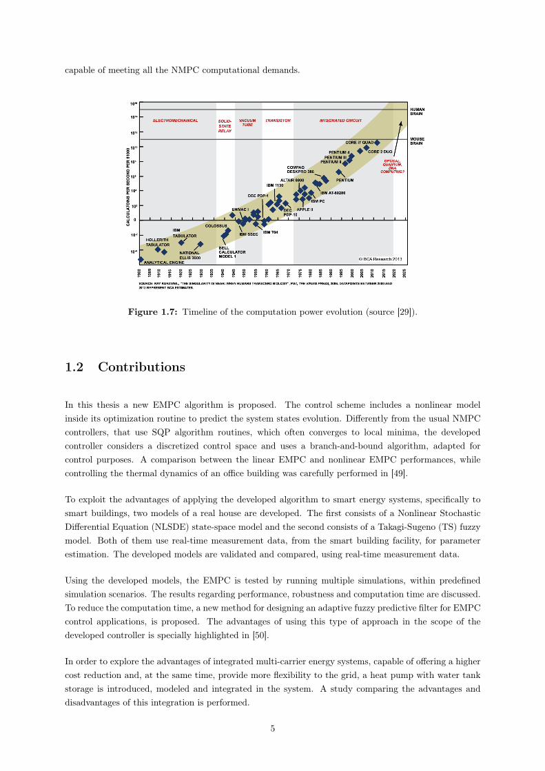
capable of meeting all the NMPC computational demands.
Figure 1.7: Timeline of the computation power evolution (source [29]).
1.2 Contributions
In this thesis a new EMPC algorithm is proposed. The control scheme includes a nonlinear modelinside its optimization routine to predict the system states evolution. Differently from the usual NMPCcontrollers, that use SQP algorithm routines, which often converges to local minima, the developedcontroller considers a discretized control space and uses a branch-and-bound algorithm, adapted forcontrol purposes. A comparison between the linear EMPC and nonlinear EMPC performances, whilecontrolling the thermal dynamics of an office building was carefully performed in [49].
To exploit the advantages of applying the developed algorithm to smart energy systems, specifically tosmart buildings, two models of a real house are developed. The first consists of a Nonlinear StochasticDifferential Equation (NLSDE) state-space model and the second consists of a Takagi-Sugeno (TS) fuzzymodel. Both of them use real-time measurement data, from the smart building facility, for parameterestimation. The developed models are validated and compared, using real-time measurement data.
Using the developed models, the EMPC is tested by running multiple simulations, within predefinedsimulation scenarios. The results regarding performance, robustness and computation time are discussed.To reduce the computation time, a new method for designing an adaptive fuzzy predictive filter for EMPCcontrol applications, is proposed. The advantages of using this type of approach in the scope of thedeveloped controller is specially highlighted in [50].
In order to explore the advantages of integrated multi-carrier energy systems, capable of offering a highercost reduction and, at the same time, provide more flexibility to the grid, a heat pump with water tankstorage is introduced, modeled and integrated in the system. A study comparing the advantages anddisadvantages of this integration is performed.
5

An MPC framework for MATLAB, including the developed models, the branch-and-bound optimizationroutine for MPC applications and the fuzzy predictive filtering, was developed in the scope of this thesis.
A linear EMPC version of the proposed algorithm is presented in [63] and the challenges regarding theimplementation of this advanced control technique are explored. The data analysis and the forecastanalysis are the author’s main contributions in the referred paper.
A summary of the overall work developed in this thesis and the highlights of its main contributions tothe energy field is presented in [48].
1.3 Outline
The manuscript is organized as follows:
Chapter 2 – Data Analysis for Smart Buildings
In this chapter a project development approach, for this thesis, based on intelligent data analysis isproposed. Specifically, topics such as project and data understanding, data preprocessing and the choicefor a suitable sampling time for the system, are explored.
Chapter 3 – Modeling
The first principle approach for modeling heat transfer phenomena, which is usually applied to de-scribe building thermal dynamics, is highlighted in this chapter. The building considered in this workis presented and the modeling procedure, for both Nonlinear Stochastic Differential Equation (NLSDE)state-space model and Takagi-Sugeno (TS) fuzzy model, are carefully described and validated.
Chapter 4 – Economic Model Predictive Control
This chapter presents a theoretical overview on classical MPC. Moreover, the EMPC formulation ispresented and the key differences from the traditional MPC are pointed out. A nonlinear EMPC algorithmis designed, based on the models developed in Chapter 3, and its performance assessment is presented,by analyzing the related simulations. Additionally, the feasibility under uncertain scenarios is ensured,by introducing a soft-constraints formulation. The performance is also improved, by the integration of anew fuzzy predictive filtering approach, for EMPC applications in the smart energy systems field.
Chapter 5 – Coupling Electricity and Heating via Heat Pump Integration
In this chapter it is proposed an integration of an electricity-heating system, together with the buildingpresented in Chapter 3. This system consists of a domestic heat pump, with and a hot water tank, andis modeled using a white-box modeling approach. The EMPC developed in Chapter 4 is used to control
6

the integrated system in a centralized fashion and the energetic assessment, comparing the performance,with and without the heat pump with hot water tank, is presented.
Chapter 6 – Conclusion
The final chapter provides the most pertinent results and recommends some topics for future work.
7

Chapter 2
Data Analysis for Smart Buildings
The data analysis process is carefully described in this chapter. In Section 2.1, an approach for the projectdevelopment and organization, based on intelligent data analysis, is proposed. The project understandingand the motivation for data understanding are addressed in Section 2.2. Section 2.3 describes the datapreprocessing. Finally, Section 2.4 performs an analysis that allows to determine a suitable samplingtime for the system.
2.1 Intelligent Data Analysis
Together with the technological advancements, data is becoming more and more important in any projectdevelopment. Within the big data paradigm, nowadays it is possible to “feel” data flowing throughdifferent means, in the most different formats and shapes. Hence, each project will be different from eachother and, as mentioned in [16], some human intelligent interference is always a need in a data-dependentproject. This intelligent approach allows the project designer to maximize the knowledge extraction, fromthe collected data.
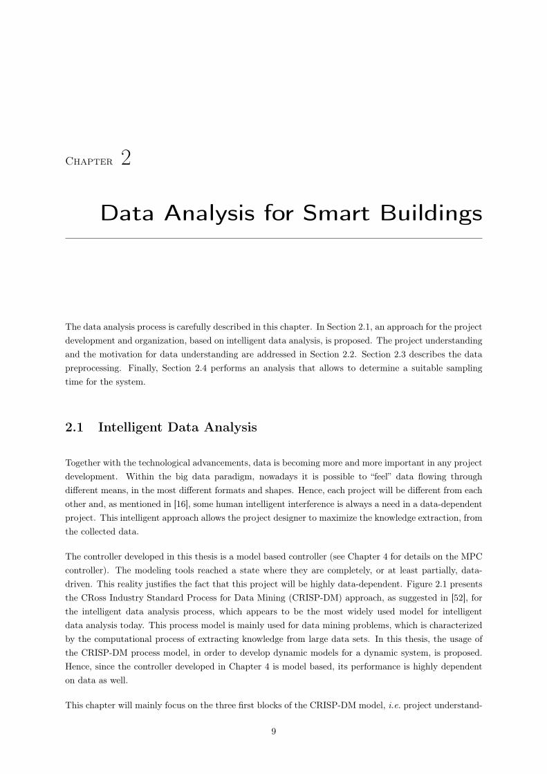
The controller developed in this thesis is a model based controller (see Chapter 4 for details on the MPCcontroller). The modeling tools reached a state where they are completely, or at least partially, data-driven. This reality justifies the fact that this project will be highly data-dependent. Figure 2.1 presentsthe CRoss Industry Standard Process for Data Mining (CRISP-DM) approach, as suggested in [52], forthe intelligent data analysis process, which appears to be the most widely used model for intelligentdata analysis today. This process model is mainly used for data mining problems, which is characterizedby the computational process of extracting knowledge from large data sets. In this thesis, the usage ofthe CRISP-DM process model, in order to develop dynamic models for a dynamic system, is proposed.Hence, since the controller developed in Chapter 4 is model based, its performance is highly dependenton data as well.
This chapter will mainly focus on the three first blocks of the CRISP-DM model, i.e. project understand-
9
ing, data understanding and data preparation. The modeling phase, together with its related evaluation,will be addressed in Chapter 3.
ProjectUnderstanding
DataUnderstanding
partially
does datasuit theproblem?
no
cancelproject
yes
DataPreparation
partially
Modeling
likely
technicalquality
improvable?unlikely
Evaluation objectiveachieved?
no
closeproject
success
Deployment
Figure 2.1: Overview of the CRISP-DM process.
2.2 Project and Data Understanding
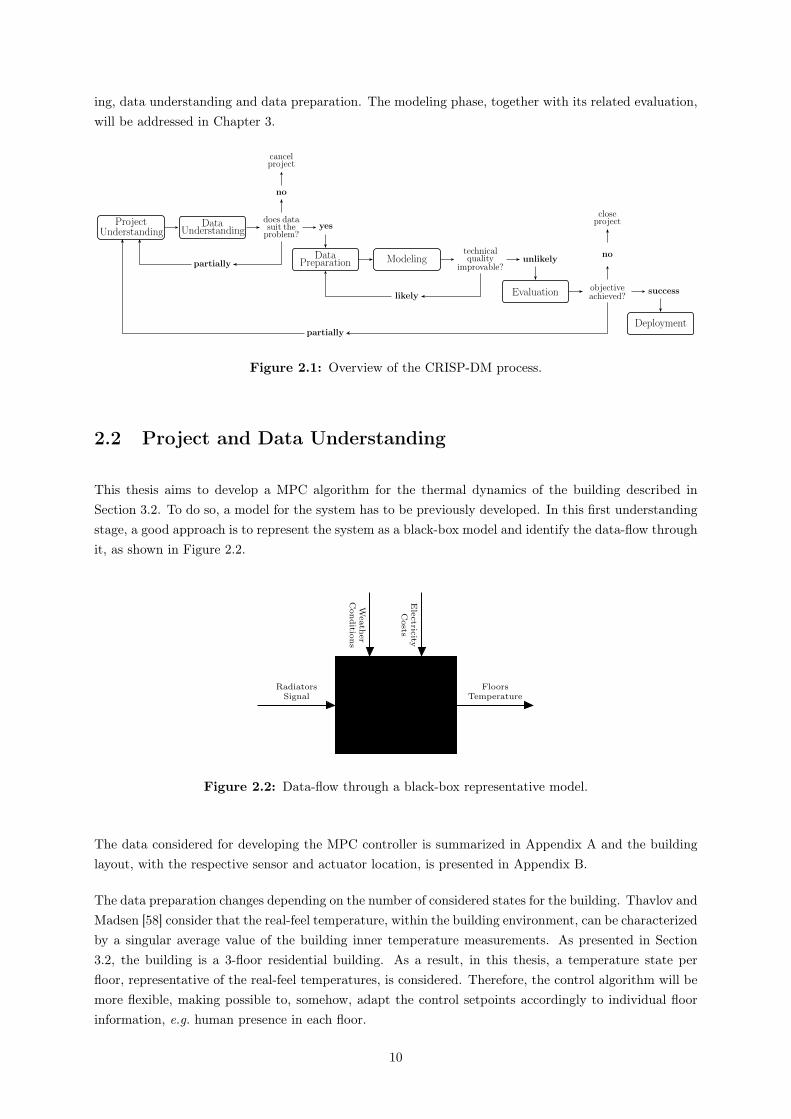
This thesis aims to develop a MPC algorithm for the thermal dynamics of the building described inSection 3.2. To do so, a model for the system has to be previously developed. In this first understandingstage, a good approach is to represent the system as a black-box model and identify the data-flow throughit, as shown in Figure 2.2.
RadiatorsSignal
FloorsTemperature
Electric
ityCosts
Weath
er
Conditio
ns
Figure 2.2: Data-flow through a black-box representative model.
The data considered for developing the MPC controller is summarized in Appendix A and the buildinglayout, with the respective sensor and actuator location, is presented in Appendix B.
The data preparation changes depending on the number of considered states for the building. Thavlov andMadsen [58] consider that the real-feel temperature, within the building environment, can be characterizedby a singular average value of the building inner temperature measurements. As presented in Section3.2, the building is a 3-floor residential building. As a result, in this thesis, a temperature state perfloor, representative of the real-feel temperatures, is considered. Therefore, the control algorithm will bemore flexible, making possible to, somehow, adapt the control setpoints accordingly to individual floorinformation, e.g. human presence in each floor.
10
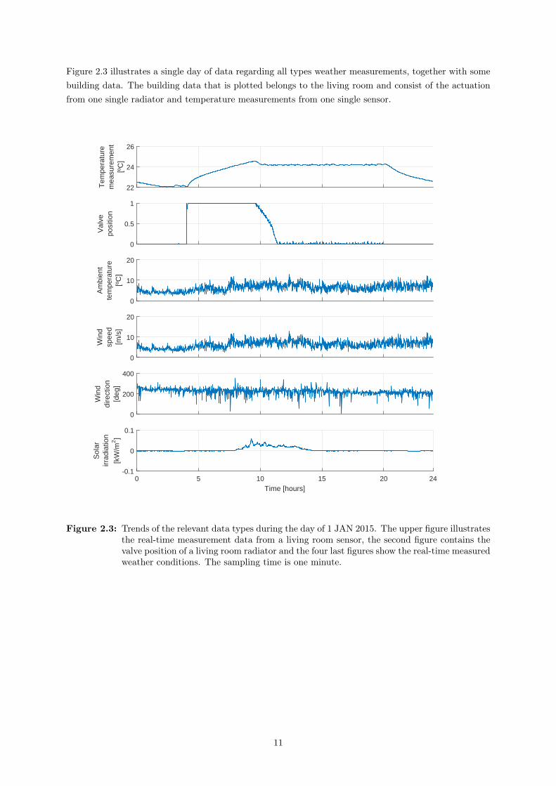
Figure 2.3 illustrates a single day of data regarding all types weather measurements, together with somebuilding data. The building data that is plotted belongs to the living room and consist of the actuationfrom one single radiator and temperature measurements from one single sensor.
22
24
26
Tem
pera
ture
mea
sure
men
t[º
C]
0
0.5
1
Val
vepo
sitio
n
0
10
20
Am
bien
tte
mpe
ratu
re[º
C]
0
10
20
Win
dsp
eed
[m/s
]
0
200
400
Win
ddi
rect
ion
[deg
]
0 5 10 15 20 24
Time [hours]
-0.1
0
0.1
Sol
arirr
adia
tion
[kW
/m2]
Figure 2.3: Trends of the relevant data types during the day of 1 JAN 2015. The upper figure illustratesthe real-time measurement data from a living room sensor, the second figure contains thevalve position of a living room radiator and the four last figures show the real-time measuredweather conditions. The sampling time is one minute.
11

2.3 Data Preprocessing
2.3.1 Measurement Data
2.3.1.1 Weather Data
The weather conditions have a big influence on the system dynamics. In the present thesis it is assumedthat only the ambient temperature, the wind speed, wind direction and the solar irradiation have di-rect influence on the building’s thermal dynamics. Some measurements are highly corrupted with highfrequency noise inherent to the sensors themselves, as it is observable in Figure 2.3. To overcome thereferred issue, a Butterworth Filter [6] was used to eliminate the present high frequency noise from thedata set.
The Nyquist Sampling Theorem, introduced in [40], states that the sampling rate that allows the recoveryof all the frequency components of a certain signal is half of the sample rate. Accordingly to the samplingtime ts, selected in Section 2.4, the cutoff frequency ωn is given by
ωn =ωs2
=π
ts= 0.0035 rad/s (2.1)
where ωs represents the sampling frequency in rad/s.
With the appropriate cutoff frequency determined, the 5th order low-pass Butterworth Filter was de-signed. Its representative transfer function is described as follows:
H(z) =B(z)
A(z)=
=4.93× 10⁻¹² + 2.47× 10⁻¹¹ z−1 + 4.93× 10⁻¹¹ z−2 + 4.93× 10⁻¹¹ z−3 + 2.47× 10⁻¹¹ z−4 + 4.93× 10⁻¹² z−5
1− 4.96 z−1 + 9.86 z−2 − 9.79 z−3 + 4.86 z−4 − 0.97 z−5.
(2.2)
Figures 2.4, 2.5, 2.6 and 2.7 represent the full data set which, after filtering and removing missing valuesand outliers, is equivalent, in quantity, to a period of one year (mixed data set with data from 2014 and2015) and was collected from the SYALAB [43] weather station.
12
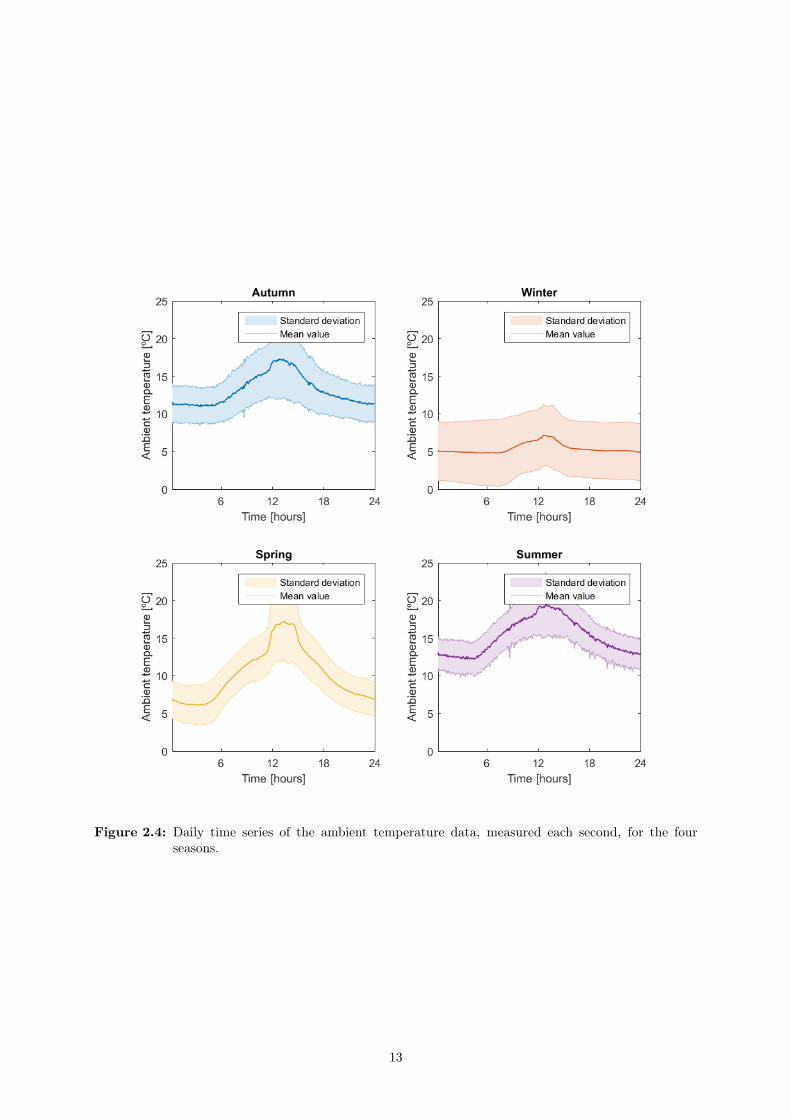
Figure 2.4: Daily time series of the ambient temperature data, measured each second, for the fourseasons.
13
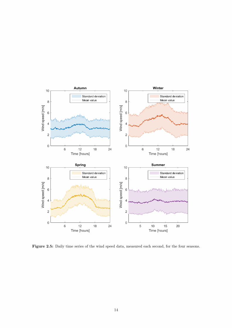
Figure 2.5: Daily time series of the wind speed data, measured each second, for the four seasons.
14
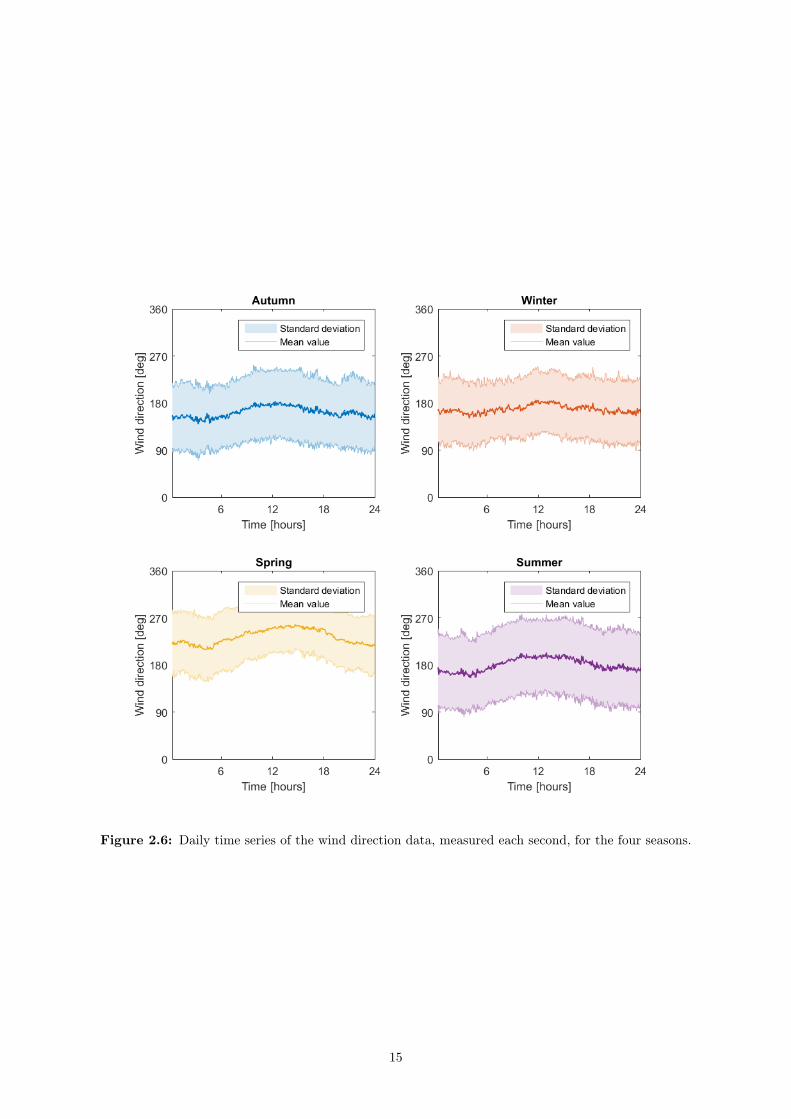
Figure 2.6: Daily time series of the wind direction data, measured each second, for the four seasons.
15
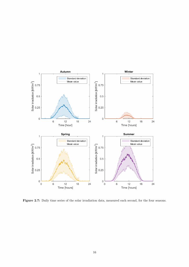
Figure 2.7: Daily time series of the solar irradiation data, measured each second, for the four seasons.
16
2.3.1.2 Building Data
As it can be observed in the building hardware layout contained in Appendix B, each floor has morethan one temperature sensor and more than one radiator. Hence, it is necessary to, somehow, group thetemperature measurements and radiator input signals of each floor. It can be noticed that the sensors werecarefully placed away from the heat sources, what ensures that the measured temperatures are similarto the real-feel temperatures. Therefore, the measurements of each floor, i.e. radiator input signals andtemperature measurements, are going to be grouped using the average operator. It is assumed that bothtoilet and stairs measurements are not relevant for each floor’s average real-feel temperature estimationand, due to that, these sensors were not included in this grouping.
The complete data set, after removing missing value periods and outliers, consists in temperature mea-surements and radiator input signals, from an equivalent period of one year, sampled each minute. Duringthis period, the system was operating within a controlled environment consisting in a thermostatic con-troller, developed by [56], which uses an independent Proportional Integrative Derivative (PID) controllerfor each room.
2.3.2 Experimental Data
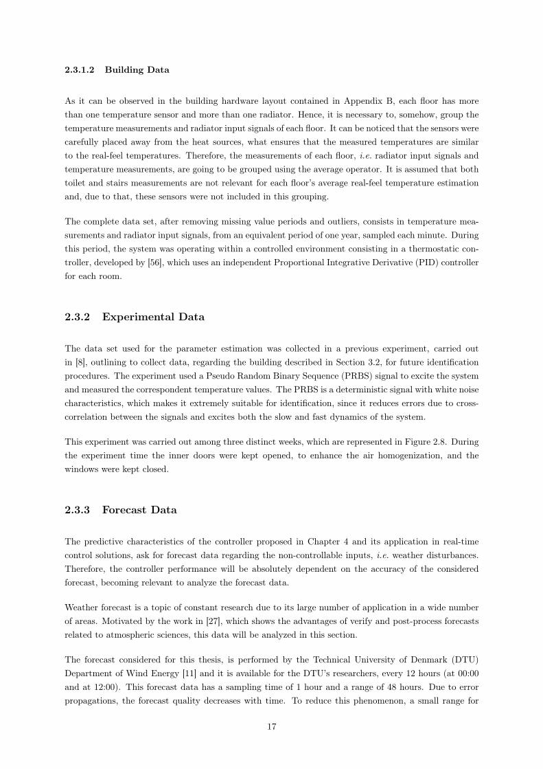
The data set used for the parameter estimation was collected in a previous experiment, carried outin [8], outlining to collect data, regarding the building described in Section 3.2, for future identificationprocedures. The experiment used a Pseudo Random Binary Sequence (PRBS) signal to excite the systemand measured the correspondent temperature values. The PRBS is a deterministic signal with white noisecharacteristics, which makes it extremely suitable for identification, since it reduces errors due to cross-correlation between the signals and excites both the slow and fast dynamics of the system.
This experiment was carried out among three distinct weeks, which are represented in Figure 2.8. Duringthe experiment time the inner doors were kept opened, to enhance the air homogenization, and thewindows were kept closed.
2.3.3 Forecast Data
The predictive characteristics of the controller proposed in Chapter 4 and its application in real-timecontrol solutions, ask for forecast data regarding the non-controllable inputs, i.e. weather disturbances.Therefore, the controller performance will be absolutely dependent on the accuracy of the consideredforecast, becoming relevant to analyze the forecast data.
Weather forecast is a topic of constant research due to its large number of application in a wide numberof areas. Motivated by the work in [27], which shows the advantages of verify and post-process forecastsrelated to atmospheric sciences, this data will be analyzed in this section.
The forecast considered for this thesis, is performed by the Technical University of Denmark (DTU)Department of Wind Energy [11] and it is available for the DTU’s researchers, every 12 hours (at 00:00and at 12:00). This forecast data has a sampling time of 1 hour and a range of 48 hours. Due to errorpropagations, the forecast quality decreases with time. To reduce this phenomenon, a small range for
17
0 1 2 3 4 5 6
Time [days]
10
15
20
25
30T
empe
ratu
rem
easu
rem
ent
[ºC
]Tb
Tf1
Tf2
0 1 2 3 4 5 6
Time [days]
0
0.2
0.4
0.6
0.8
1
Ele
ctric
rad
iato
r si
gnal
hb
hf1
hf2
0 1 2 3 4 5 6 7
Time [days]
15
20
25
30
35
Tem
pera
ture
mea
sure
men
t[º
C]
Tb
Tf1
Tf2
0 1 2 3 4 5 6 7
Time [days]
0
0.2
0.4
0.6
0.8
1
Ele
ctric
rad
iato
r si
gnal
hb
hf1
hf2
0 1 2 3 4 5 6
Time [days]
15
20
25
30
Tem
pera
ture
mea
sure
men
t[º
C]
Tb
Tf1
Tf2
0 1 2 3 4 5 6
Time [days]
0
0.2
0.4
0.6
0.8
1
Ele
ctric
rad
iato
r si
gnal
hb
hf1
hf2
Figure 2.8: Data collected during the PRBS experiment. The first figure illustrates the period of 8 to15 APR 2013, the second illustrates the period of 2 to 9 MAY 2013 and third illustratesthe period of 8 to 15 MAY 2013. The sampling time is one minute.
each forecast, which at the same time ensures that there is no missing information within the controlalgorithm, i.e. 12 hours forecast range, will be considered for this thesis.
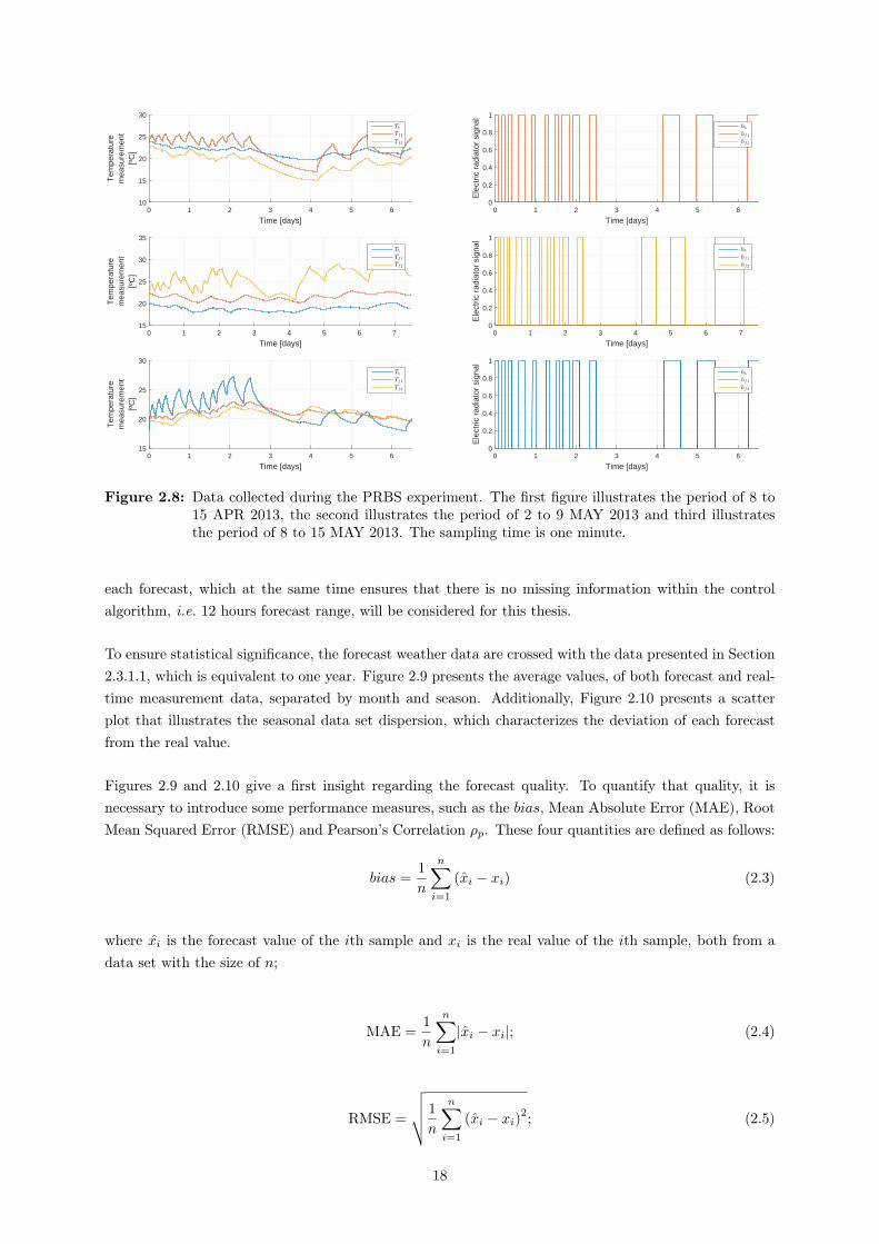
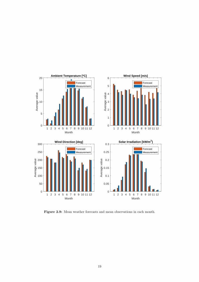
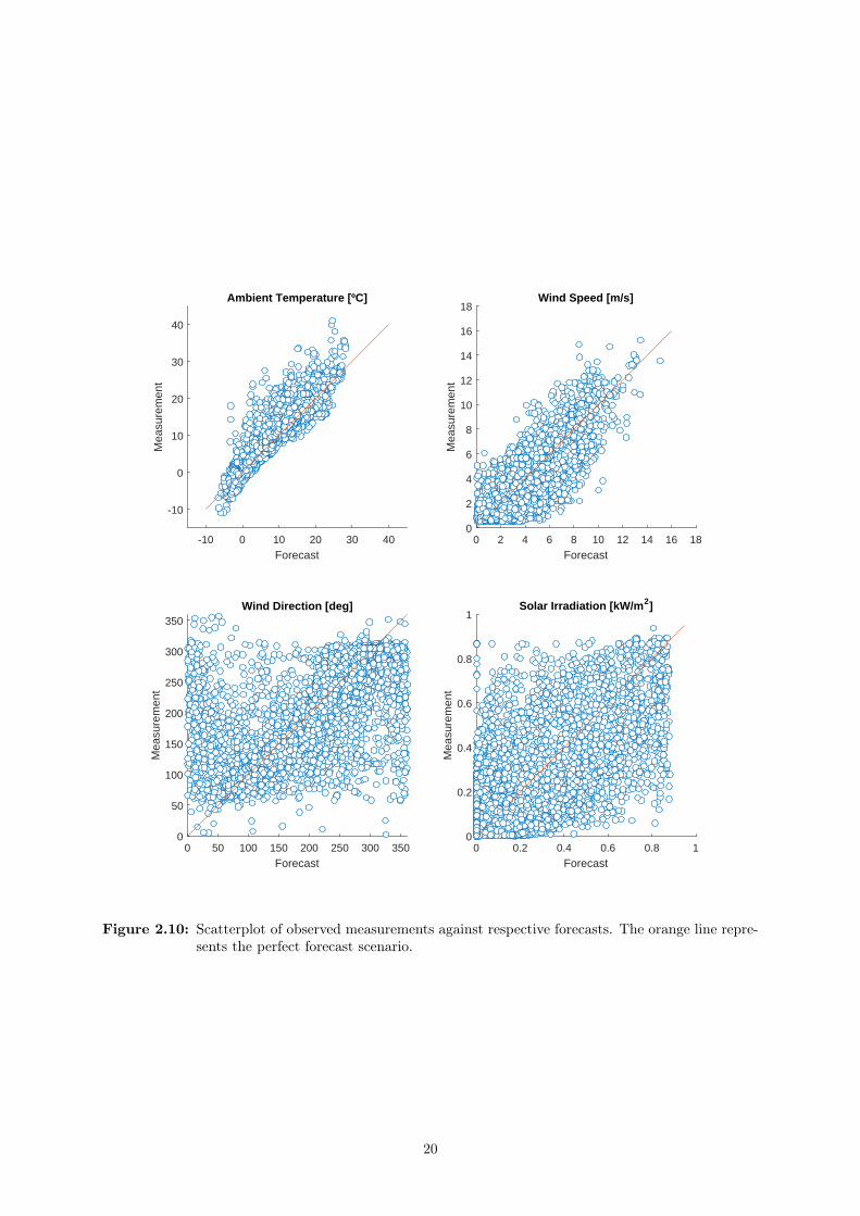
To ensure statistical significance, the forecast weather data are crossed with the data presented in Section2.3.1.1, which is equivalent to one year. Figure 2.9 presents the average values, of both forecast and real-time measurement data, separated by month and season. Additionally, Figure 2.10 presents a scatterplot that illustrates the seasonal data set dispersion, which characterizes the deviation of each forecastfrom the real value.
Figures 2.9 and 2.10 give a first insight regarding the forecast quality. To quantify that quality, it isnecessary to introduce some performance measures, such as the bias, Mean Absolute Error (MAE), RootMean Squared Error (RMSE) and Pearson’s Correlation ρp. These four quantities are defined as follows:
bias =1
n
n∑i=1
(xi − xi) (2.3)
where xi is the forecast value of the ith sample and xi is the real value of the ith sample, both from adata set with the size of n;
MAE =1
n
n∑i=1
|xi − xi|; (2.4)
RMSE =
√√√√ 1
n
n∑i=1
(xi − xi)2; (2.5)
18
1 2 3 4 5 6 7 8 9 10 11 12
Month
0
5
10
15
20
Ave
rage
val
ue
Ambient Temperature [ºC]
ForecastMeasurement
1 2 3 4 5 6 7 8 9 10 11 12
Month
0
0.05
0.1
0.15
0.2
0.25
0.3
Ave
rage
val
ue
Solar Irradiation [kW/m 2]
ForecastMeasurement
1 2 3 4 5 6 7 8 9 10 11 12
Month
0
1
2
3
4
5
6
Ave
rage
val
ue
Wind Speed [m/s]
ForecastMeasurement
1 2 3 4 5 6 7 8 9 10 11 12
Month
0
50
100
150
200
250
300
Ave
rage
val
ue
Wind Direction [deg]
ForecastMeasurement
Figure 2.9: Mean weather forecasts and mean observations in each month.
19
-10 0 10 20 30 40
Forecast
-10
0
10
20
30
40
Mea
sure
men
t
Ambient Temperature [ºC]
0 0.2 0.4 0.6 0.8 1
Forecast
0
0.2
0.4
0.6
0.8
1
Mea
sure
men
t
Solar Irradiation [kW/m 2]
0 2 4 6 8 10 12 14 16 18
Forecast
0
2
4
6
8
10
12
14
16
18
Mea
sure
men
t
Wind Speed [m/s]
0 50 100 150 200 250 300 350
Forecast
0
50
100
150
200
250
300
350
Mea
sure
men
t
Wind Direction [deg]
Figure 2.10: Scatterplot of observed measurements against respective forecasts. The orange line repre-sents the perfect forecast scenario.
20
ρp =cov(x, x)√
var(x) var(x)(2.6)
where the cov(x, x) can be estimated using the equation (2.7). The variances can be also estimated usingthe relations var(x) = cov(x, x) and var(x) = cov(x, x).
cov(x, x) =1
n
n∑i=1
(xi − xi)(xi − xi
). (2.7)
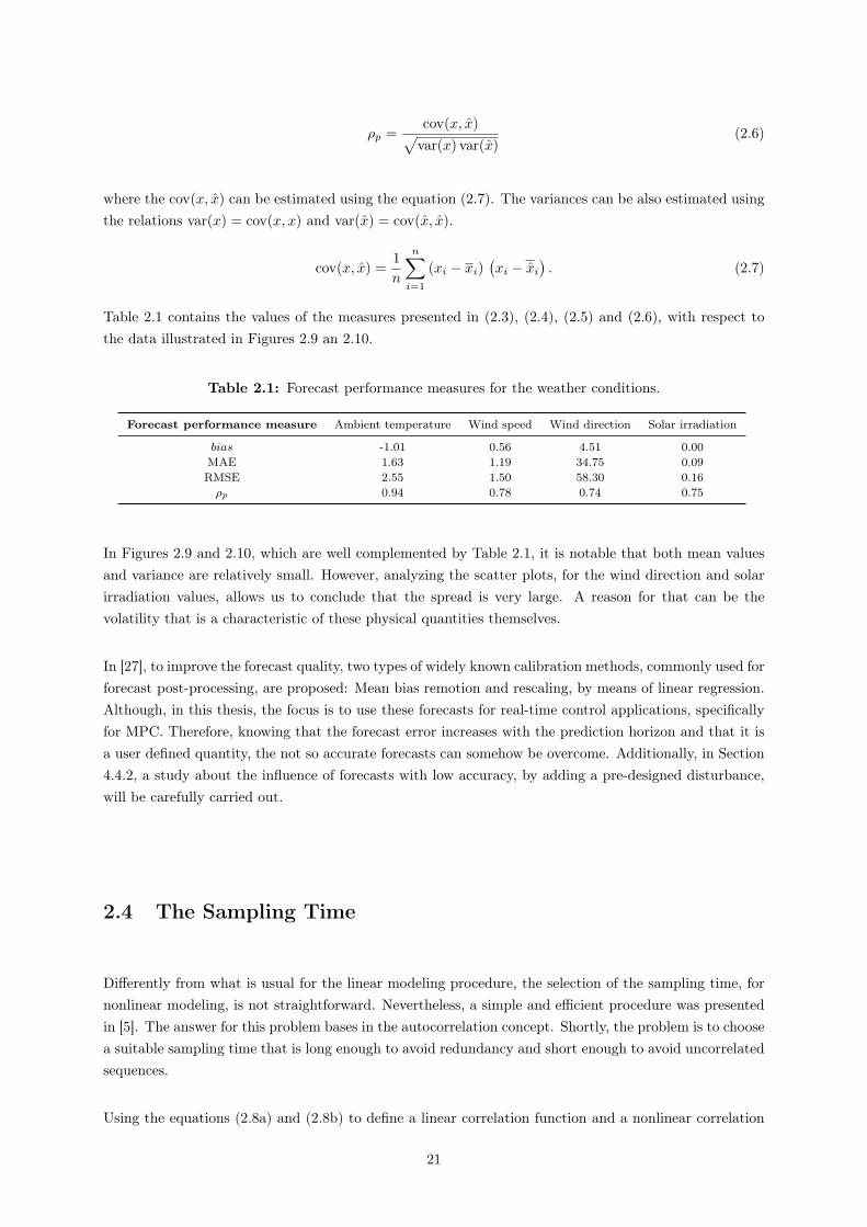
Table 2.1 contains the values of the measures presented in (2.3), (2.4), (2.5) and (2.6), with respect tothe data illustrated in Figures 2.9 an 2.10.
Table 2.1: Forecast performance measures for the weather conditions.
Forecast performance measure Ambient temperature Wind speed Wind direction Solar irradiation
bias -1.01 0.56 4.51 0.00MAE 1.63 1.19 34.75 0.09RMSE 2.55 1.50 58.30 0.16ρp 0.94 0.78 0.74 0.75
In Figures 2.9 and 2.10, which are well complemented by Table 2.1, it is notable that both mean valuesand variance are relatively small. However, analyzing the scatter plots, for the wind direction and solarirradiation values, allows us to conclude that the spread is very large. A reason for that can be thevolatility that is a characteristic of these physical quantities themselves.
In [27], to improve the forecast quality, two types of widely known calibration methods, commonly used forforecast post-processing, are proposed: Mean bias remotion and rescaling, by means of linear regression.Although, in this thesis, the focus is to use these forecasts for real-time control applications, specificallyfor MPC. Therefore, knowing that the forecast error increases with the prediction horizon and that it isa user defined quantity, the not so accurate forecasts can somehow be overcome. Additionally, in Section4.4.2, a study about the influence of forecasts with low accuracy, by adding a pre-designed disturbance,will be carefully carried out.
2.4 The Sampling Time
Differently from what is usual for the linear modeling procedure, the selection of the sampling time, fornonlinear modeling, is not straightforward. Nevertheless, a simple and efficient procedure was presentedin [5]. The answer for this problem bases in the autocorrelation concept. Shortly, the problem is to choosea suitable sampling time that is long enough to avoid redundancy and short enough to avoid uncorrelatedsequences.
Using the equations (2.8a) and (2.8b) to define a linear correlation function and a nonlinear correlation
21
function, respectively, it is possible to detect the two kinds of correlation in a certain data sequence y(k).
Ryy(τc) = E[(y(k)− y(k)
) (y(k − τc)− y(k)
)](2.8a)
Ry2′y2′ (τc) = E[(y2(k)− y2(k)
) (y2(k − τc)− y2(k)
)](2.8b)
where τc is the time-lag.
Accordingly to the information contained in the quantities expressed in equations (2.8), the first localminimum of Ryy, namely τy, and the first local minimum of Ry2′y2′ , namely τy2′ , can be used in equation(2.9) to determine the faster local minimum τm between the linear and nonlinear dynamics.
τm = minτy, τy2′
. (2.9)
The sampling time is chosen in order to respect the equation given by
τm20≤ ts ≤
τm10. (2.10)
To apply the described procedure to this work, the three data sets collected for the experiment presentedin Section 2.3.2, will be used for the sampling time study. These data contains information of the fasterdynamics, which is the critical information for the sampling time selection.
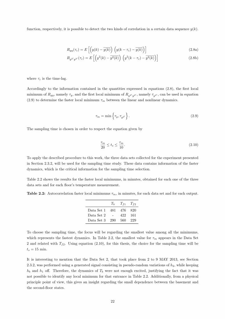
Table 2.2 shows the results for the faster local minimums, in minutes, obtained for each one of the threedata sets and for each floor’s temperature measurement.
Table 2.2: Autocorrelation faster local minimums τm, in minutes, for each data set and for each output.
Tb Tf1 Tf2
Data Set 1 481 476 820Data Set 2 - 422 161Data Set 3 290 560 229
To choose the sampling time, the focus will be regarding the smallest value among all the minimums,which represents the fastest dynamics. In Table 2.2, the smallest value for τm appears in the Data Set2 and related with Tf2. Using equation (2.10), for this thesis, the choice for the sampling time will bets = 15 min.
It is interesting to mention that the Data Set 2, that took place from 2 to 9 MAY 2013, see Section2.3.2, was performed using a generated signal consisting in pseudo-random variations of h2, while keepinghb and h1 off. Therefore, the dynamics of Tb were not enough excited, justifying the fact that it wasnot possible to identify any local minimum for that entrance in Table 2.2. Additionally, from a physicalprinciple point of view, this gives an insight regarding the small dependence between the basement andthe second-floor states.
22
Chapter 3
Modeling
This chapter describes the full modeling process carried out for this thesis. Section 3.1 introduces thedifferent heat transfer mechanisms and modes, using a first principle approach. After that, in Section 3.2,the building is described and its thermal dynamics is analyzed. Using the physics presented in Section3.1, Section 3.3 is focused on the development of a Stochastic Differential Equations (SDE) state-spacemodel. In Section 3.4, a Takagi-Sugeno (TS) fuzzy modeling is carefully described. Finally, Section 3.5presents discussion regarding the developed models.
3.1 Heat Transfer Phenomena
There are uncountable ways of describing the phenomena of heat transfer. An intuitive way to do it,as mentioned in [4], is to interpret it as a physical transport phenomena that exchanges thermal energyfrom one emitter to a receiver through a specific heat transfer mode. These modes are described withmore detail in the following subsections. Moreover, the heat transfer, as a thermal process, is ruled bythe Laws of Thermodynamics.
Particularly, in a building, the three fundamental modes of heat transfer play notable roles in its heatdynamics. These modes are referred to conduction, convection and radiation.
3.1.1 Conduction
This mode of heat transfer occurs when there is a temperature gradient in a stationary medium, i.e. solidor fluid. It happens at atomic/molecular level and due to the interactions between the more energeticand the less energetic particles, while the macroscopic movement state of the medium is stopped. Theseinteractions are frequently collisions or diffusion in fluids and vibrations in solids.
23
The heat conduction phenomenon is described by the Fourier’s Law, which is given by
q′′cond = −kcond∇T = −kcond(
i∂T
∂x+ j
∂T
∂y+ k
∂T
∂z
)(3.1)
where the heat flux vector q′′cond is the heat transfer rate per unit of area, kcond is a physical propertycalled thermal conductivity (quantifies the rate at which energy is transferred), and T (x, y, z) is the scalartemperature field. The negative sign in the Equation (3.1) suggests that the heat transfer respects theSecond Law of Thermodynamics, which states that the temperature flow occurs from the high temperaturelevel to the low temperature level.
Based in the First Law of Thermodynamics, i.e. conservation of energy, applying it to an infinitesimalsmall control volume and recalling the Fourier’s Law introduced in (3.1), it is possible to introduce therelated heat inflows and outflows obtaining the so called Heat Diffusion Equation formulated as
ρm cp∂T
∂t= qg +∇ · (kcond∇T ) = qg +
∂
∂x
(kcond
∂T
∂x
)+
∂
∂y
(kcond
∂T
∂y
)+
∂
∂z
(kcond
∂T
∂z
)(3.2)
with ρm being the mass density of the material, cp the specific heat capacity and qg the rate of thermalenergy generation within the medium. The previous equation provides the basic tool for heat conductionanalysis. From its solution, it is possible to determine the temperature distribution T (x, y, z) as a functionof time.
The case of the heat transfer through a wall becomes much simpler than the general case. It is assumedthat the heat flow is normal to the wall, that is in a steady state condition and that there is no energygeneration within the wall. Using Equations (3.1) and (3.2), the heat rate equation is expressed by
qcondx =kcondA
L(Ts,i − Ts,o) (3.3)
where L is the thickness of the wall, A is the area of the wall normal to the direction of heat transfer andthe inside wall surface temperature Ts,i is assumed to be higher than the outside surface temperatureTs,o.
Usually the walls are composed by different kind of layers, there is a need to introduce a formulation forthe composite wall heat transfer problem. This is made extending the relation (3.3) defining the overallheat transfer coefficient U , consisting in the sum of each wall portion i. The heat rate equation for a wallcomposed by Nwl different layers is given by
qcondx =1∑Nwl−1
i=1Li
kcondiA
(Ts,i − Ts,o) = UA∆T. (3.4)
24
3.1.2 Convection
Differently from conduction, the convection heat transfer mode is observed when a fluid is in motion andbounded by a surface, in addiction to the presence of a temperature gradient between the two. Thisheat transfer mode is based, not only in the mechanism pointed out in Section 3.1.1, i.e. the diffusionphenomenon, but also in an additional foundation promoted by the macroscopic motion of the fluidparticles as a whole group. Convection is then the term that is widely used to define this kind ofcumulative heat transfer phenomenon.
The convective heat transfer can be classified according to the nature of the flow. If the flow is causedby external sources (e.g. fan, pump, atmospheric wind) it is often called forced convection. Differently,if the flow is caused by buoyancy forces, which are due to the density heterogeneousness caused by thetemperature gradient, it is called free convection (e.g. bolling water, hot air balloon).
However, the fact that it is possible to have conditions consisting in mixed types of convection, i.e. freeand forced, added to the high heterogeneous properties of the fluid such as densities and relative velocities,makes convection a very complex phenomena.
The Newton’s Law of Cooling characterizes this mode of heat transfer and is give by
q′′conv = hconv (Tsur − T∞) (3.5)
where the convective heat transfer rate per unit of area q′′conv is given by the product of the convectionheat transfer coefficient hconv with the difference between the surface temperature Tsur and the fluidtemperature T∞. The relation (3.5) is defined positive if the heat transfer has the direction from thesurface to the fluid.
The convection heat transfer coefficient is a property that, used together with the Newton’s Law ofCooling, can reduce the complexity of the heat transfer phenomena to the characterization of hconv.Although, this property is highly dependent on the boundary layer conditions, that are influenced bygeometry, fluid motion, thermodynamic and transport laws, which sometimes make the heat transferproblem just solvable resorting Computational Fluid Dynamics (CFD) methods.
3.1.3 Radiation
All the matter above the minimum absolute temperature emits thermal energy through radiation mode.The physical principle basically consists in the transport by means of electromagnetic waves due tochanges in the electron configurations of the constituent atoms and molecules. Radiation can occurwithout the presence of a material medium between the source and the receiver, being more efficient ina vacuum.
The Stefan-Boltzmann Law quantifies the heat transfer rate emitted by a surface due to radiation as
q′′rad = ε σSB T4sur (3.6)
25
with the radiation heat transfer rate per unit of area q′′rad being dependent on the emissivity ε ∈ [0, 1]
and on the Stefan-Boltzmann constant σSB = 5.67 × 10⁻⁸ W/m2 · K4. The emissivity measures howefficiently a certain surface emits energy relative to the perfect emitter, i.e. the blackbody.
A frequent special case occurs, which consists in radiation exchange between a small surface and a muchlarger isothermal surface, surrounding the first one. Assuming that this surface is a gray surface, i.e. itabsorbs radiation as good as it emits, the following equation, yields
q′′rad = ε σSB(T 4sur − T 4
rad
)(3.7)
which represents the balance between the thermal energy emitted and absorbed by means of radiation.
Sometimes it is possible to measure the solar irradiation power ΦS directly. Once done that, the heattransfer rate per unit of area q′′rad = ΦS can directly be determined.
3.2 The Building: PowerFlexhouse 3
The PowerFlexhouse 3 is a 150 m2 3-floor intelligent residential building, shown in the Fig. 3.1, which islocated at DTU Risø Campus, in Roskilde.
(a) Front facade. (b) Back facade.
Figure 3.1: Facades of the PowerFlexhouse 3.
The building brick walls have a layer of insulation between them. Appendix B presents a layout, containingthe hardware location, in the house.
The building’s heating system is composed by a set of water-based radiators that can be controlledindividually and using continuous control signals between 0 and 1, which correspond to the valve opening.For more detail regarding the heating system output power distribution within the building, see AppendixC.
26
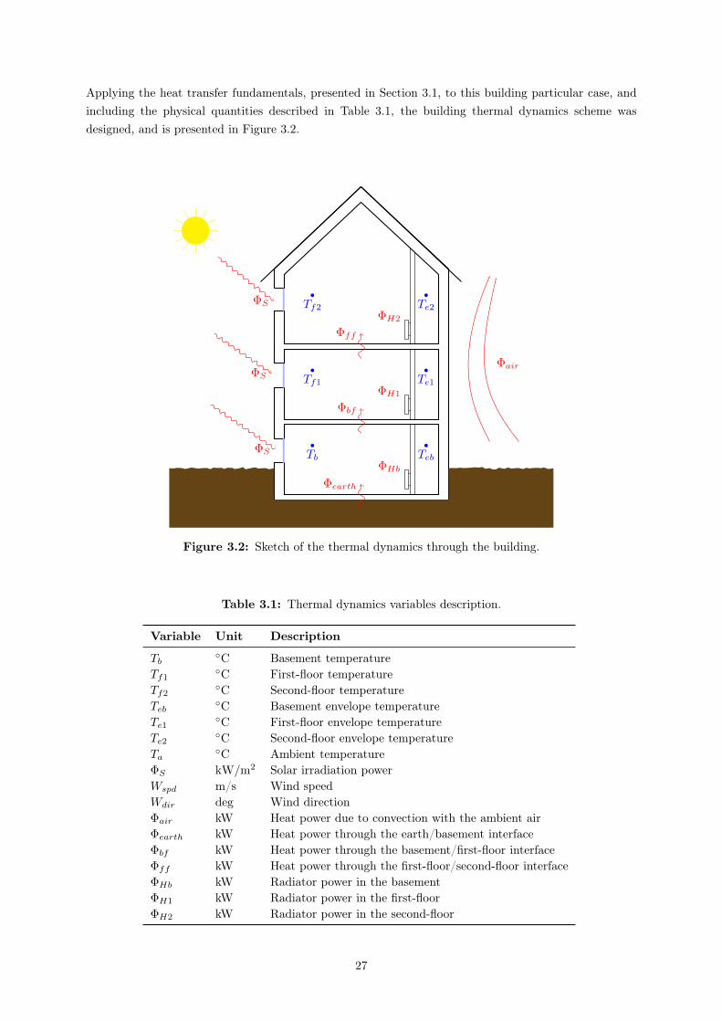
Applying the heat transfer fundamentals, presented in Section 3.1, to this building particular case, andincluding the physical quantities described in Table 3.1, the building thermal dynamics scheme wasdesigned, and is presented in Figure 3.2.
ΦS
ΦS
ΦS
ΦH2
ΦH1
ΦHb
Tf2
Tf1
Tb
Te2
Te1
Teb
Φff
Φbf
Φearth
Φair
Figure 3.2: Sketch of the thermal dynamics through the building.
Table 3.1: Thermal dynamics variables description.
Variable Unit Description
TbC Basement temperature
Tf1C First-floor temperature
Tf2C Second-floor temperature
TebC Basement envelope temperature
Te1C First-floor envelope temperature
Te2C Second-floor envelope temperature
TaC Ambient temperature
ΦS kW/m2 Solar irradiation powerWspd m/s Wind speedWdir deg Wind directionΦair kW Heat power due to convection with the ambient airΦearth kW Heat power through the earth/basement interfaceΦbf kW Heat power through the basement/first-floor interfaceΦff kW Heat power through the first-floor/second-floor interfaceΦHb kW Radiator power in the basementΦH1 kW Radiator power in the first-floorΦH2 kW Radiator power in the second-floor
27

3.3 Stochastic Differential Equations State-Space Model
It is well known that Nonlinear Stochastic Differential Equations (NLSDE) [41], when used in the contextof a continuous-discrete stochastic state-space model, based both on classical dynamical Ordinary Differ-ential Equations (ODE)-modeling and stochastic modeling, represents one of the most powerful tools tobuild models of dynamical systems.
In the general case, the continuous-discrete stochastic state-space model considering the state vector xt,the input vector ut and the parameter vector θ is given by
dxt = fSDE(xt,ut, t,θ)dt+ σ(ut, t,θ)dωt (3.8a)
yk = hSDE(xk,uk, tk,θ) + ek (3.8b)
where t ∈ IR is the time variable; k is a discrete sampling time; fSDE(·) is a nonlinear function called thedrift term; σ(·) is the diffusion term of the process; hSDE(·) is a nonlinear function linking the statesand the measured output yk; ωt is a standard Wiener process; ek is the observation noise characterizedby the white noise process with ek ∈ N(0,σ2
0(uk, tk,θ)).
The first step to model a system by the analytical grey-box approach is to use first principles and priorphysical knowledge to build the proper NLSDE system. In this case, the model will be formulated as alumped system, described by the Resistor-Capacitor (RC) equivalent circuit diagram illustrated in Figure3.3, considering the following assumptions:
(1) The temperature is spatially homogeneous in each considered state;
(2) The heaters are modeled as resistance heaters and they can be seen as a direct input of heat into thesystem;
(3) Only the solar radiation incident in the main windows have significant contributions, regarding energytransferred by radiation, to the energy balance equations;
(4) The convection is not considered for the basement states dynamics;
(5) The convection heat transfer coefficient can change with the wind speed and the wind direction;
(6) The remaining thermal properties are constants.
Hence, according to the system described in Figure 3.2, together with the help of the RC equivalentcircuit presented in Figure 3.3, the continuous-discrete stochastic state-space model for the system takes
28
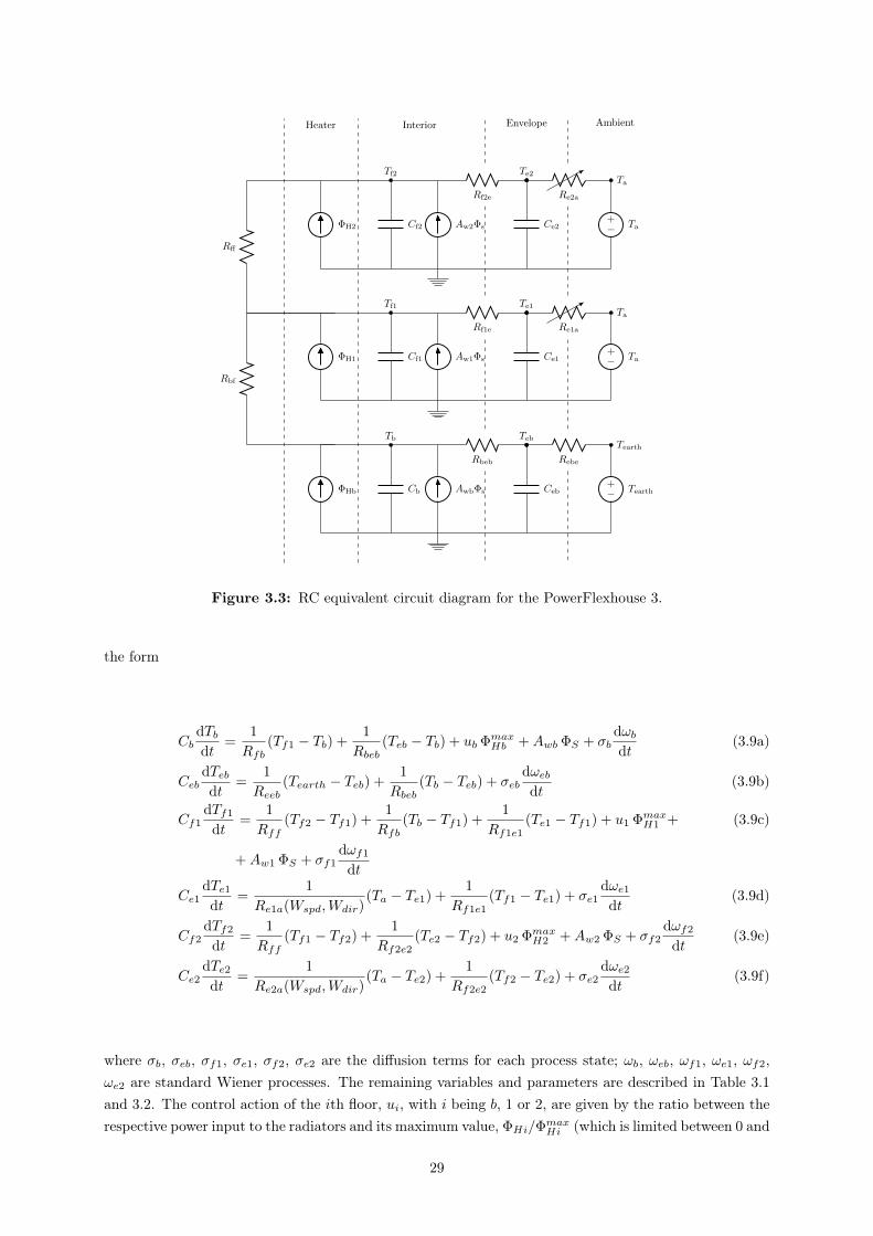
ΦH2
ΦH1
ΦHb
Cf2
Tf2
Aw2Φs
Rf2e
Cf1
Tf1
Aw1Φs
Rf1e
Cb
Tb
AwbΦs
Rbeb
Ce2
Te2
Re2a
Ce1
Te1
Re1a
Ceb
Teb
Rebe
+− Ta
Ta
+− Ta
Ta
+− Tearth
Tearth
Heater Interior Envelope Ambient
Rff
Rbf
Figure 3.3: RC equivalent circuit diagram for the PowerFlexhouse 3.
the form
CbdTbdt
=1
Rfb(Tf1 − Tb) +
1
Rbeb(Teb − Tb) + ub ΦmaxHb +Awb ΦS + σb
dωbdt
(3.9a)
CebdTebdt
=1
Reeb(Tearth − Teb) +
1
Rbeb(Tb − Teb) + σeb
dωebdt
(3.9b)
Cf1dTf1
dt=
1
Rff(Tf2 − Tf1) +
1
Rfb(Tb − Tf1) +
1
Rf1e1(Te1 − Tf1) + u1 ΦmaxH1 + (3.9c)
+Aw1 ΦS + σf1dωf1
dt
Ce1dTe1dt
=1
Re1a(Wspd,Wdir)(Ta − Te1) +
1
Rf1e1(Tf1 − Te1) + σe1
dωe1dt
(3.9d)
Cf2dTf2
dt=
1
Rff(Tf1 − Tf2) +
1
Rf2e2(Te2 − Tf2) + u2 ΦmaxH2 +Aw2 ΦS + σf2
dωf2
dt(3.9e)
Ce2dTe2dt
=1
Re2a(Wspd,Wdir)(Ta − Te2) +
1
Rf2e2(Tf2 − Te2) + σe2
dωe2dt
(3.9f)
where σb, σeb, σf1, σe1, σf2, σe2 are the diffusion terms for each process state; ωb, ωeb, ωf1, ωe1, ωf2,ωe2 are standard Wiener processes. The remaining variables and parameters are described in Table 3.1and 3.2. The control action of the ith floor, ui, with i being b, 1 or 2, are given by the ratio between therespective power input to the radiators and its maximum value, ΦHi/Φ
maxHi (which is limited between 0 and
29

1). Notice that the model is a nonlinear model, since the terms Re1a(Wspd,Wdir) and Re2a(Wspd,Wdir)
are functions of two inputs and are on the denominator.
An appropriate function for the resistances was found, using some knowledge regarding heat transfer andfluid mechanics theory. In a general way, the power function cW W γW
spd is used to express the relationbetween the resistances and the wind speed, see e.g. [9, 26, 58]. In this work, to improve the results ofthe resistance estimation, an extension to this correlation was proposed, taking into account both windspeed and wind direction. Using the potential flow theory together with a simple geometric analysis ofthe building, the relations (3.10a) and (3.10b) were developed.
Re1a(Wspd,Wdir) = cW1 [Wspd (|sin (Wdir + θ0)|+ |cos (Wdir + θ0)|)]γW1 (3.10a)
Re2a(Wspd,Wdir) = cW2 [Wspd (|sin (Wdir + θ0)|+ |cos (Wdir + θ0)|)]γW2 . (3.10b)
3.3.1 Parameter Estimation – Maximum Likelihood Estimator
Defined the model structure, there is a need to perform the estimation of the model parameters. Thisestimation will be performed using the Maximum Likelihood Estimator (MLE) [36], that has been suc-cessfully applied to identification problems.
The MLE is a method that fits the Gaussian probability distribution that makes the observed datay = [y(0) . . . y(t− 1) y(t)]
T most likely. Assuming that the observation vector y is constituted only bystatistically independent processes, the joint probability density function can be given by
f(y, θ) =
N∏i=1
fi(yi,θ) (3.11)
where N is the number of observations in the output vector y, fi is the probability density function ofan observation yi at a certain time instant and θ is the unknown true parameter vector.
The likelihood function can now be described as shown in the equation (3.12). The method seeks theestimated parameter vector θ that maximizes the likelihood function L(θ).
L(θ) ≡ L(θ;y) = f(y, θ) = p(y | θ). (3.12)
Once the stochastic processes ω and e presented in (3.8a) and (3.8b) follow Gaussian distributions, theyare completely described by their mean and covariance. Hence we characterize the conditional densityby the same statistical properties mentioned above.
y(k | k − 1) = E [y(k) | y(k − 1),θ)] (3.13a)
R(k | k − 1) = V [y(k) | y(k − 1),θ)] (3.13b)
30
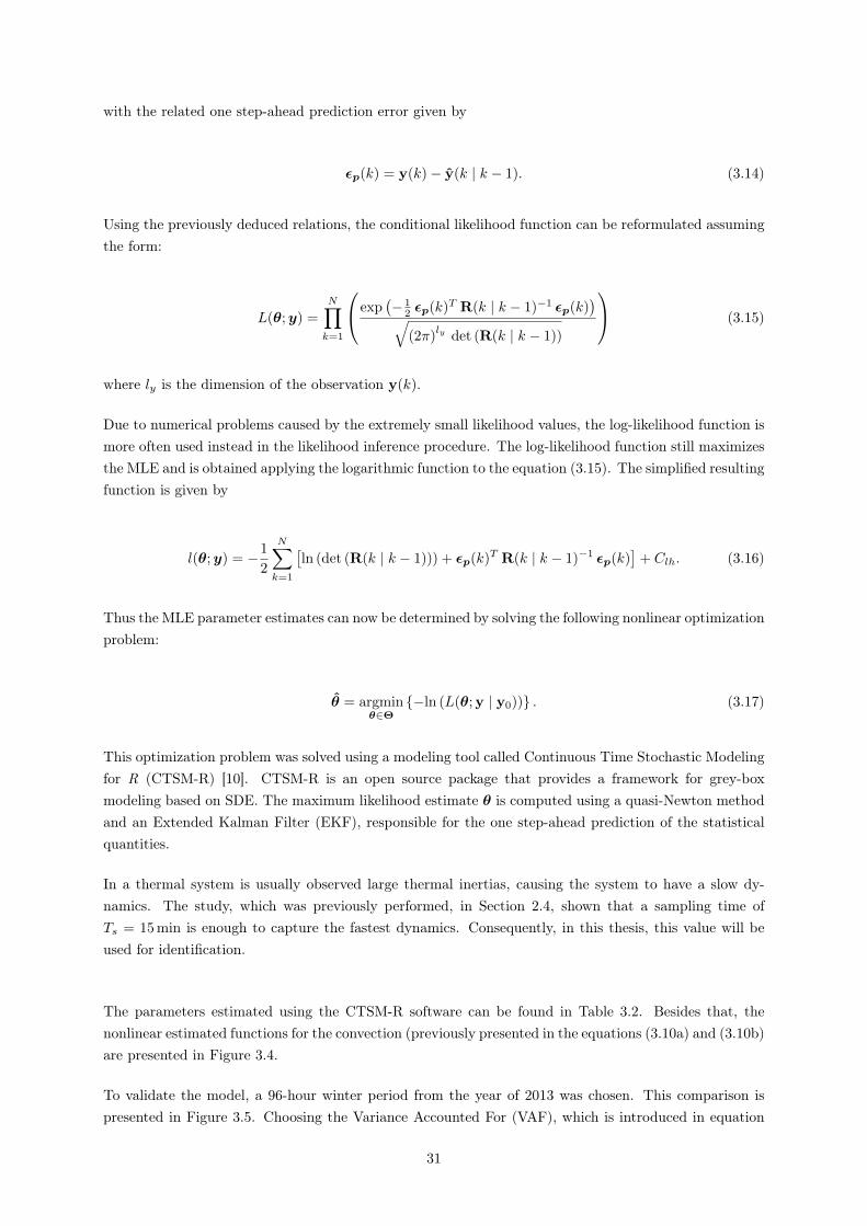
with the related one step-ahead prediction error given by
εp(k) = y(k)− y(k | k − 1). (3.14)
Using the previously deduced relations, the conditional likelihood function can be reformulated assumingthe form:
L(θ;y) =
N∏k=1
exp(− 1
2 εp(k)T R(k | k − 1)−1 εp(k))√
(2π)ly det (R(k | k − 1))
(3.15)
where ly is the dimension of the observation y(k).
Due to numerical problems caused by the extremely small likelihood values, the log-likelihood function ismore often used instead in the likelihood inference procedure. The log-likelihood function still maximizesthe MLE and is obtained applying the logarithmic function to the equation (3.15). The simplified resultingfunction is given by
l(θ;y) = −1
2
N∑k=1
[ln (det (R(k | k − 1))) + εp(k)T R(k | k − 1)−1 εp(k)
]+ Clh. (3.16)
Thus the MLE parameter estimates can now be determined by solving the following nonlinear optimizationproblem:
θ = argminθ∈Θ
−ln (L(θ; y | y0)) . (3.17)
This optimization problem was solved using a modeling tool called Continuous Time Stochastic Modelingfor R (CTSM-R) [10]. CTSM-R is an open source package that provides a framework for grey-boxmodeling based on SDE. The maximum likelihood estimate θ is computed using a quasi-Newton methodand an Extended Kalman Filter (EKF), responsible for the one step-ahead prediction of the statisticalquantities.
In a thermal system is usually observed large thermal inertias, causing the system to have a slow dy-namics. The study, which was previously performed, in Section 2.4, shown that a sampling time ofTs = 15 min is enough to capture the fastest dynamics. Consequently, in this thesis, this value will beused for identification.
The parameters estimated using the CTSM-R software can be found in Table 3.2. Besides that, thenonlinear estimated functions for the convection (previously presented in the equations (3.10a) and (3.10b)are presented in Figure 3.4.
To validate the model, a 96-hour winter period from the year of 2013 was chosen. This comparison ispresented in Figure 3.5. Choosing the Variance Accounted For (VAF), which is introduced in equation
31
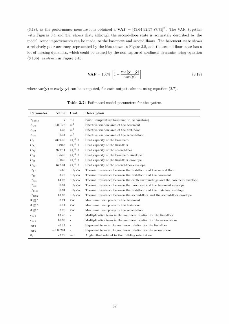
(3.18), as the performance measure it is obtained a VAF = [43.64 92.57 87.75]T . The VAF, together
with Figures 3.4 and 3.5, shows that, although the second-floor state is accurately described by themodel, some improvements can be made, to the basement and second floors. The basement state showsa relatively poor accuracy, represented by the bias shown in Figure 3.5, and the second-floor state has alot of missing dynamics, which could be caused by the non captured nonlinear dynamics using equation(3.10b), as shown in Figure 3.4b.
VAF = 100%
[1− var (y − y)
var (y)
](3.18)
where var(y) = cov(y,y) can be computed, for each output column, using equation (2.7).
Table 3.2: Estimated model parameters for the system.
Parameter Value Unit Description
Tearth 7 C Earth temperature (assumed to be constant)
Awb 0.00176 m2 Effective window area of the basement
Aw1 1.35 m2 Effective window area of the first-floor
Aw2 0.44 m2 Effective window area of the second-floor
Cb 7399.40 kJ/C Heat capacity of the basement
Cf1 14955 kJ/C Heat capacity of the first-floor
Cf2 9727.1 kJ/C Heat capacity of the second-floor
Ceb 12540 kJ/C Heat capacity of the basement envelope
Ce1 13040 kJ/C Heat capacity of the first-floor envelope
Ce2 672.31 kJ/C Heat capacity of the second-floor envelope
Rff 5.60 C/kW Thermal resistance between the first-floor and the second floor
Rfb 3.73 C/kW Thermal resistance between the first-floor and the basement
Reeb 14.25 C/kW Thermal resistance between the earth surroundings and the basement envelope
Rbeb 0.84 C/kW Thermal resistance between the basement and the basement envelope
Rf1e1 0.31 C/kW Thermal resistance between the first-floor and the first-floor envelope
Rf2e2 13.95 C/kW Thermal resistance between the second-floor and the second-floor envelope
ΦmaxHb 2.71 kW Maximum heat power in the basement
ΦmaxH1 6.14 kW Maximum heat power in the first-floor
ΦmaxH2 2.20 kW Maximum heat power in the second-floor
cW1 13.40 - Multiplicative term in the nonlinear relation for the first-floor
cW2 10.93 - Multiplicative term in the nonlinear relation for the second-floor
γW1 -0.14 - Exponent term in the nonlinear relation for the first-floor
γW2 −0.00281 - Exponent term in the nonlinear relation for the second-floor
θ0 -2.28 rad Angle offset related to the building orientation
32
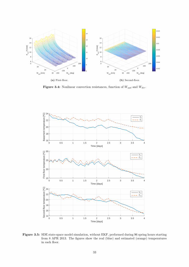
62000
8
10
10010
Re1
a [º
C/k
W]
12
Wspd
[m/s] Wdir
[deg]
0
14
20
16
-100-20030
8
9
10
11
12
13
14
(a) First-floor.
60 200
8
10
10010
Re2
a [º
C/k
W]
12
Wdir
[deg]Wspd
[m/s]
0
14
20
16
-100-20030
10.82
10.84
10.86
10.88
10.9
10.92
10.94
(b) Second-floor.
Figure 3.4: Nonlinear convection resistances, function of Wspd and Wdir.
0 0.5 1 1.5 2 2.5 3 3.5 4
Time [days]
16
18
20
22
24
Bas
emen
t tem
pera
ture
[ºC
]
Tb
Tb
0 0.5 1 1.5 2 2.5 3 3.5 4
Time [days]
15
20
25
30
Firs
t-flo
or te
mpe
ratu
re [º
C]
Tf1
Tf1
0 0.5 1 1.5 2 2.5 3 3.5 4
Time [days]
14
16
18
20
22
24
Sec
ond-
floor
tem
pera
ture
[ºC
]
Tf2
Tf2
Figure 3.5: SDE state-space model simulation, without EKF, performed during 96 spring hours startingfrom 8 APR 2013. The figures show the real (blue) and estimated (orange) temperaturesin each floor.
33
3.3.2 Extended Kalman Filter
In the results shown in Figure 3.5, it is notable that there is unmodeled dynamics with appreciableimportance in the system behavior. In order to decrease that importance and increase the accuracy ofthe model presented in this section, an hybrid version of the EKF will be formulated and applied to thatcontinuous-discrete stochastic state-space model. This EKF is going to be used, together with measuringupdates after each 2 hours, to increase the model performance.
A version of Kalman Filter [28] that extends its range of applications to nonlinear models was initiallyproposed by [7]. Since then, this particular adaptation named EKF is the most widely used estimationalgorithm for nonlinear systems.
Considering the continuous-time dynamics and discrete-time measurements described by equations (3.8),the Hybrid EKF is introduced by writing the first-order Taylor expansion which takes the form
dxt ≈[f(xt,ut, t,θ) + A(t)(xt − xt|k)
]dt+ σ(ut, t,θ)dωt (3.19)
where the Jacobian A(t) = ∂f(x,ut,t,θ)∂x
∣∣∣x=xt|k
is used to approximate the nonlinear function.
Based on the linearization described in equation (3.19) and on an Algebraic Riccati Equation (ARE), theapproximate solution for the equation (3.19) was derived and is given by,
˙xt|k = f(xt,ut, t,θ) (3.20a)
Pt|k = A(t) Pt|k + Pt|k A(t)T + σ(ut, t,θ)σ(ut, t,θ)T (3.20b)
with initial conditions x0 = E[xtk ] and P0 = E[(x0− x0)(x0− x0)T ], for the state vector and covariancematrix, respectively.
Last, at each measurement time, the state estimate and the covariance matrix should be updated asfollows:
Kk = Pk|k−1 CTk
(Ck Pk|k−1 CT
k + σ20(uk, tk,θ)
)−1(3.21a)
xk|k = xk|k−1 + Kk
(yk − yk|k−1
)(3.21b)
Pk|k = Pk|k−1 −Kk
(Ck Pk|k−1 CT
k + σ20(uk, tk,θ)
)KTk (3.21c)
where Ck represents the output matrix. The quantities A(t) and Ck, for the model of the systempresented in (3.9), can be found in Appendix D.
This presented equations (3.19), (3.20) and (3.21) can be solved iteratively, using the numerical methodsused by the ODE solvers.
3.3.3 Model Validation
The model presented in Section 3.3 was validated using measurement data, different from the one usedfor the identification process described in Section 3.3.1. The model should describe the system, in aconsistent and accurate way, not only during a specific season, but in every season. To ensure that, a30-day batch per season was used for validation.
34
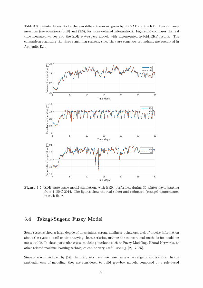
Table 3.3 presents the results for the four different seasons, given by the VAF and the RMSE performancemeasures (see equations (3.18) and (2.5), for more detailed information). Figure 3.6 compares the realtime measured values and the SDE state-space model, with incorporated hybrid EKF results. Thecomparison regarding the three remaining seasons, since they are somehow redundant, are presented inAppendix E.1.
0 5 10 15 20 25 30
Time [days]
20
22
24
26
Bas
emen
t tem
pera
ture
[ºC
]
Tb
Tb
0 5 10 15 20 25 30
Time [days]
18
20
22
24
26
Firs
t-flo
or te
mpe
ratu
re [º
C]
Tf1
Tf1
0 5 10 15 20 25 30
Time [days]
16
18
20
22
24
Sec
ond-
floor
tem
pera
ture
[ºC
]
Tf2
Tf2
Figure 3.6: SDE state-space model simulation, with EKF, performed during 30 winter days, startingfrom 1 DEC 2014. The figures show the real (blue) and estimated (orange) temperaturesin each floor.
3.4 Takagi-Sugeno Fuzzy Model
Some systems show a large degree of uncertainty, strong nonlinear behaviors, lack of precise informationabout the system itself or time varying characteristics, making the conventional methods for modelingnot suitable. In these particular cases, modeling methods such as Fuzzy Modeling, Neural Networks, orother related machine learning techniques can be very useful, see e.g. [2, 17, 55].
Since it was introduced by [62], the fuzzy sets have been used in a wide range of applications. In theparticular case of modeling, they are considered to build grey-box models, composed by a rule-based
35
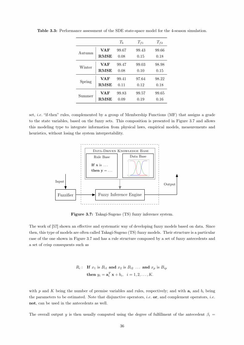
Table 3.3: Performance assessment of the SDE state-space model for the 4-season simulation.
Tb Tf1 Tf2
AutumnVAF 99.67 99.43 99.66RMSE 0.08 0.15 0.18
WinterVAF 99.47 99.03 98.98RMSE 0.08 0.10 0.15
SpringVAF 99.41 97.64 98.22RMSE 0.11 0.12 0.18
SummerVAF 99.83 99.57 99.65RMSE 0.09 0.19 0.16
set, i.e. “if-then” rules, complemented by a group of Membership Functions (MF) that assigns a gradeto the state variables, based on the fuzzy sets. This composition is presented in Figure 3.7 and allowsthis modeling type to integrate information from physical laws, empirical models, measurements andheuristics, without losing the system interpretability.
Fuzzifier Fuzzy Inference Engine
Rule Base
If x is . . .
then y = . . .
Data Base
0
1
InputOutput
Data-Driven Knowledge Base
Figure 3.7: Takagi-Sugeno (TS) fuzzy inference system.
The work of [57] shown an effective and systematic way of developing fuzzy models based on data. Sincethen, this type of models are often called Takagi-Sugeno (TS) fuzzy models. Their structure is a particularcase of the one shown in Figure 3.7 and has a rule structure composed by a set of fuzzy antecedents anda set of crisp consequents such as
Ri : If x1 is Bi1 and x2 is Bi2 . . . and xp is Bip
then yi = aTi x + bi, i = 1, 2, . . . ,K.
with p and K being the number of premise variables and rules, respectively; and with ai and bi beingthe parameters to be estimated. Note that disjunctive operators, i.e. or, and complement operators, i.e.not, can be used in the antecedents as well.
The overall output y is then usually computed using the degree of fulfillment of the antecedent βi =
36
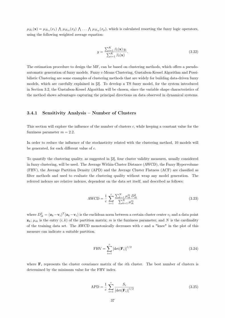
µBi(x) = µBi1
(x1)∧µBi2
(x2)∧. . .∧µBip
(xp), which is calculated resorting the fuzzy logic operators,using the following weighted average equation:
y =
∑Ki=1 βi(x) yi∑Ki=1 βi(x)
. (3.22)
The estimation procedure to design the MF, can be based on clustering methods, which offers a pseudo-automatic generation of fuzzy models. Fuzzy c-Means Clustering, Gustafson-Kessel Algorithm and Possi-bilistic Clustering are some examples of clustering methods that are widely for building data-driven fuzzymodels, which are carefully explained in [2]. To develop a TS fuzzy model, for the system introducedin Section 3.2, the Gustafson-Kessel Algorithm will be chosen, since the variable shape characteristics ofthe method shows advantages capturing the principal directions on data observed in dynamical systems.
3.4.1 Sensitivity Analysis – Number of Clusters
This section will explore the influence of the number of clusters c, while keeping a constant value for thefuzziness parameter m = 2.2.
In order to reduce the influence of the stochasticity related with the clustering method, 10 models willbe generated, for each different value of c.
To quantify the clustering quality, as suggested in [2], four cluster validity measures, usually consideredin fuzzy clustering, will be used. The Average Within-Cluster Distance (AWCD), the Fuzzy Hypervolume(FHV), the Average Partition Density (APD) and the Average Cluster Flatness (ACF) are classified asfilter methods and used to evaluate the clustering quality without wrap any model generation. Thereferred indexes are relative indexes, dependent on the data set itself, and described as follows:
AWCD =1
c
c∑i=1
∑Nk=1 µ
mikD
2ik∑N
k=1 µmik
(3.23)
where D2ik = (zk−vi)
T (zk−vi) is the euclidean norm between a certain cluster center vi and a data pointzk; µik is the entry (i, k) of the partition matrix; m is the fuzziness parameter; and N is the cardinalityof the training data set. The AWCD monotonically decreases with c and a "knee" in the plot of thismeasure can indicate a suitable partition.
FHV =
c∑i=1
[det(Fi)]1/2 (3.24)
where Fi represents the cluster covariance matrix of the ith cluster. The best number of clusters isdetermined by the minimum value for the FHV index.
APD =1
c
c∑i=1
Si
[det(Fi)]1/2
(3.25)
37

where Si =∑k µik, ∀k, such that (zk − vi)
T F−1i (zk − vi) < 1. An appropriate number of clusters
corresponds to large values of APD.
ACF =1
c
c∑i=1
λinλi1
(3.26)
with λin and λi1 being the smallest and the largest eingenvalues of Fi, respectively. Similarly to theAPD, the minimization of the ACF index corresponds to a more suitable number of clusters choice.
The performed study is illustrated in Figure 3.8. Note that each validity measure, corresponding to acertain value of c, is an average value of 10 studies. Each column of that figure corresponds to a differentoutput, hence should be analyzed column-wise and as follows:
Tb. Accordingly to the AWCD and the APD measures, c = 5 is the appropriate number of clusters,while FHV and ACF indicate that c = 3 or c = 4 are the best parameters. With the goal ofdeveloping a simple and interpretable model, c = 3 is chosen as number of clusters.
Tf1. In this case, the "knee" for the AWCD index represents an excessively large number for c. For thisreason, this validity measure will not be considered. The remaining performance measures showconsistent information, pointing c = 3 as the best number of clusters.
Tf2. A situation similar to the Tf1 case occurred, when studying Tf2. Both AWCD and APD have localextreme values, that correspond to very large values for c. Thus, the trend of FHV and ACF andtheir local minimums, where c = 3 and c = 4, are good candidates for the parameter. Followingthe same heuristics as before, c = 3 is chosen, for the sake of simplicity.
The outcome of the sensitivity analysis performed to the c parameter is presented in Table 3.4. Eachentry represents the best values for c, regarding each output and each different cluster validity measureand according to the justification presented before.
Table 3.4: Number of clusters results, applying the cluster validity measures.
Cluster validity measure Tb Tf1 Tf2
AWCD 5 - -
FHV 3,4 3 3
APD 5 3 -
ACF 3,4 3 3
Overall 3 3 3
38
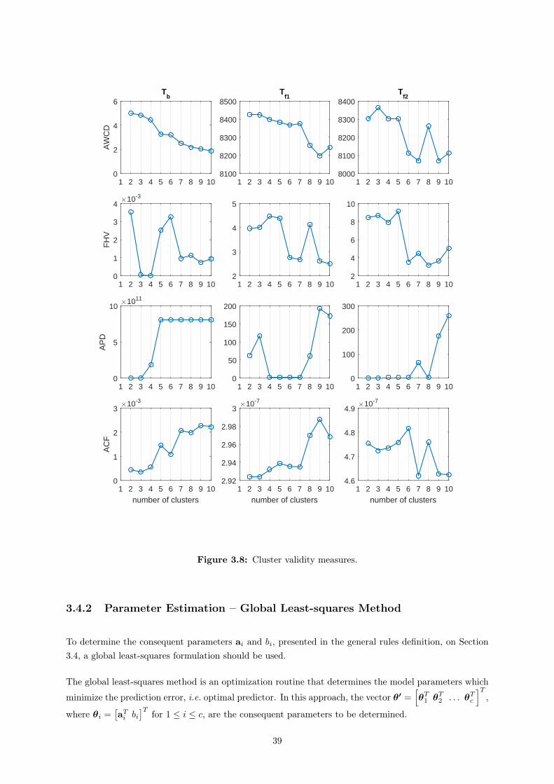
1 2 3 4 5 6 7 8 9 100
5
10
AP
D
×1011
1 2 3 4 5 6 7 8 9 100
50
100
150
200
1 2 3 4 5 6 7 8 9 100
100
200
300
1 2 3 4 5 6 7 8 9 10
number of clusters
0
1
2
3
AC
F
×10-3
1 2 3 4 5 6 7 8 9 10
number of clusters
2.92
2.94
2.96
2.98
3×10⁻⁷
1 2 3 4 5 6 7 8 9 10
number of clusters
4.6
4.7
4.8
4.9×10⁻⁷
1 2 3 4 5 6 7 8 9 100
1
2
3
4
FH
V
×10-3
1 2 3 4 5 6 7 8 9 102
3
4
5
1 2 3 4 5 6 7 8 9 102
4
6
8
10
1 2 3 4 5 6 7 8 9 100
2
4
6A
WC
D
Tb
1 2 3 4 5 6 7 8 9 108100
8200
8300
8400
8500T
f1
1 2 3 4 5 6 7 8 9 108000
8100
8200
8300
8400T
f2
Figure 3.8: Cluster validity measures.
3.4.2 Parameter Estimation – Global Least-squares Method
To determine the consequent parameters ai and bi, presented in the general rules definition, on Section3.4, a global least-squares formulation should be used.
The global least-squares method is an optimization routine that determines the model parameters which
minimize the prediction error, i.e. optimal predictor. In this approach, the vector θ′ =[θT1 θ
T2 . . . θTc
]T,
where θi =[aTi bi
]T for 1 ≤ i ≤ c, are the consequent parameters to be determined.
39

Formulating the problem in an matrix fashion, the quantity Γi should be defined as
Γi =
γi1 0 · · · 0
0 γi2 · · · 0
......
. . ....
0 0 · · · γiN
(3.27)
where γik = βik/∑cj=1 βjk is the normalized membership degree of the kth diagonal entry.
The extended regressor matrix is given by
Xe = [X 1] (3.28)
with X =[XT
1 XT2 . . . XT
N
]T .Based on equations (3.27) and (3.28), the global least-squares problem can be formulated as a minimiza-tion problem of the prediction error εp, which is characterized by
y = X′ θ′ + εp (3.29)
where X′ = [Γ1 Xe Γ2 Xe . . . ΓcXe]
The solution for the problem presented in equation (3.29) is given by
θ′ =[(X′)
TX′]−1
(X′)T
y. (3.30)
Once the problem (3.29) is solved, the consequent parameters can be directly obtained by
ai =[θ′q+1 θ
′q+2 . . . θ′q+p
]T (3.31a)
bi =[θ′q+p+1
](3.31b)
with q = (i− 1) (p+ 1).
TS fuzzy models are completely data-driven. Hence, the PRBS data, presented in Section 2.3.2 andpreviously used to identify the analytical model in Section 3.3, is not enough to derive a proper model.Thus, data from one entire year, presented in Section 2.3.1.2, was analyzed, treated and preprocessed,and is going to be used for the present modeling problem.
An open source software, called Fuzzy Identification Toolbox [3], which was developed by Prof. RobertBabuška for MATLAB, will be used to build the fuzzy model. The toolbox bases itself in the theoreticalprinciples presented in the beginning of Section 3.4, including the Gustafson-Kessel Clustering Algorithm.
40

The system illustrated in Section 3.2 is interpreted, in this modeling approach point of view, as a systemwith an input vector u = [ub u1 u2]T , a disturbance vector d = [Ta Φs Wspd Wdir]T and an outputvector y = [Tb Tf1 Tf2]T . The variables introduced to describe the system are presented in Table 3.1.
Once again, and for the same reasons highlighted in Section 2.4, the sampling time of Ts = 15 min, willbe used in the modeling problem.
The model can be structured as a Multiple-Input Multiple-Output (MIMO) system with 7 model inputsand 3 outputs. Using knowledge extracted while interpreting the system, it can be defined how the statesare related with each other. Knowing that it consists of a thermal system unit delays are used to relatethe state variables:
Tb(k + 1) = f(Tb(k), Tf1(k), ub(k)) (3.32a)
Tf1(k + 1) = f (Tb(k), Tf1(k), Tf2(k), u1(k), Ta(k),Wspd(k),Wdir(k),ΦS(k)) (3.32b)
Tf2(k + 1) = f (Tf1(k), Tf2(k), u2(k), Ta(k),Wspd(k),Wdir(k),ΦS(k)) . (3.32c)
3.4.3 Model Generation and Simplification
To develop a TS fuzzy model able to characterize the system, independently of the seasonal period,the data set for training will contain four subsets, one for each season. Hence, a variable range ofinformation, including sufficiently different disturbance profiles, is included in the training process andparameter estimation. The referred data was described in Sections 2.3.1.1 and 2.3.1.2.
Motivated by the randomness inherent to the TS fuzzy model generation, a study consisting in 30 modelgenerations, to study the consistency of the model generation, will be performed. The validation isperformed using a 30-day batch, for each seasonal period and with the same quantity as the validationdata set (the same batches that are considered in Section 3.4.4).
The mean value and variance for both VAF and RMSE, presented before in equations (3.18) and (2.5),will be computed and are presented in Table 3.5. These results shown that the model generation is veryconsistent, presenting a VAF and a RMSE with a large mean value, complemented by a low variance.Comparing the variance values for each output, i.e. floor temperature, it is notable that Tb is the one thatshows the lower values. The reason for that is the fact that, as stated in equation (3.32a), the basementstate is ”more isolated” than the other two, since it is considered that the basement does not feel theinfluence of any weather disturbance.
41

Table 3.5: Statistic properties regarding the validation of the 30 TS fuzzy models generated.
Tb Tf1 Tf2
Mean Value Variance Mean Value Variance Mean Value Variance
AutumnVAF 99.84 1.70 × 10⁻¹⁰ 99.87 1.56 × 10⁻⁷ 99.88 2.14 × 10⁻⁶
RMSE 0.05 6.20 × 10⁻¹² 0.05 1.89 × 10⁻⁸ 0.05 1.16 × 10⁻⁷
WinterVAF 99.63 5.23 × 10⁻⁹ 99.38 3.63 × 10⁻⁴ 99.10 1.65 × 10⁻³
RMSE 0.06 3.84 × 10⁻¹¹ 0.08 1.75 × 10⁻⁶ 0.11 7.59 × 10⁻⁶
SpringVAF 99.42 2.80 × 10⁻¹⁰ 98.92 7.03 × 10⁻⁵ 98.82 8.78 × 10⁻⁵
RMSE 0.11 2.65 × 10⁻¹² 0.08 8.19 × 10⁻⁸ 0.15 3.45 × 10⁻⁷
SummerVAF 99.91 1.97 × 10⁻¹⁰ 99.83 1.1 × 10⁻³ 99.92 4.42 × 10⁻⁵
RMSE 0.04 8.14 × 10⁻¹¹ 0.06 2.66 × 10⁻⁵ 0.05 5.22 × 10⁻⁶
A TS fuzzy model can now be generated. The fuzzyness parameter is considered to be m = 2.2, thenumber of clusters, for the 3 different outputs, is choose to be c = [3 3 3]
T . The MF are createdperforming the fuzzy projection of the partition matrix obtained after training the model.
Some of the MF characterizing the model were shown to be similar to the universe of discourse or verysimilar among each other. In [2] it is shown that these clusters can be removed or combined in order toobtain a faster, more simple and more easily interpretable model. The simplified model is described bythe MF illustrated in Figure 3.9 and the set of rules presented in Table 3.6. The dependences presentedbefore, in equations (3.32), do not represent the updated model, since some dependences are not presentanymore. The referred simplified model shows now the relations presented in equations (3.33).
Tb(k + 1) = f(Tb(k), Tf1(k), ub(k)) (3.33a)
Tf1(k + 1) = f (Tb(k), Tf1(k), Tf2(k), u1(k), Ta(k),Wspd(k),ΦS(k)) (3.33b)
Tf2(k + 1) = f (Tf1(k), Tf2(k), u2(k), Ta(k),Wspd(k),ΦS(k)) . (3.33c)
42
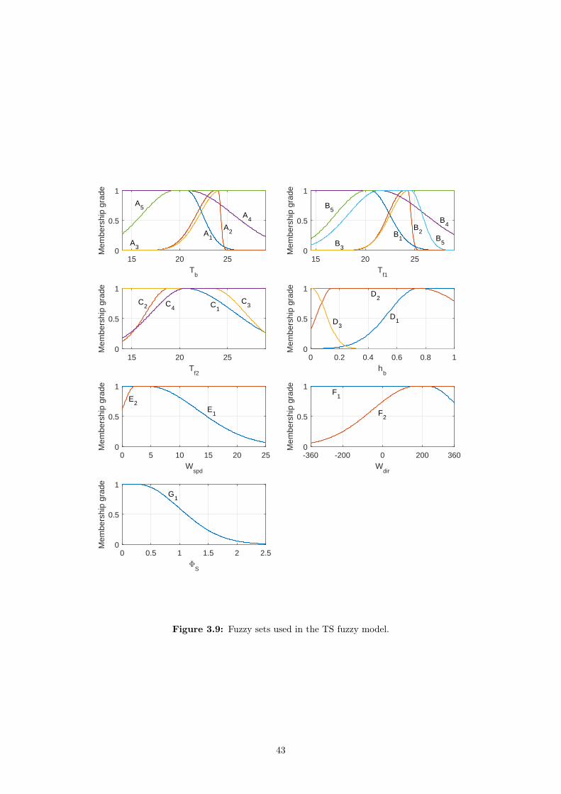
15 20 25T
b
0
0.5
1
Mem
bers
hip
grad
e
15 20 25T
f1
0
0.5
1
Mem
bers
hip
grad
e
15 20 25T
f2
0
0.5
1
Mem
bers
hip
grad
e
0 0.2 0.4 0.6 0.8 1h
b
0
0.5
1M
embe
rshi
p gr
ade
0 5 10 15 20 25W
spd
0
0.5
1
Mem
bers
hip
grad
e
-360 -200 0 200 360W
dir
0
0.5
1
Mem
bers
hip
grad
e
0 0.5 1 1.5 2 2.5Φ
S
0
0.5
1
Mem
bers
hip
grad
e
A4
A5
B4
B5
B5
C1
C2
C3C
4
D1
D2
D3
E2
F1
F2
E1
A1
A2
A3 B
3
B1
B2
G1
Figure 3.9: Fuzzy sets used in the TS fuzzy model.
43
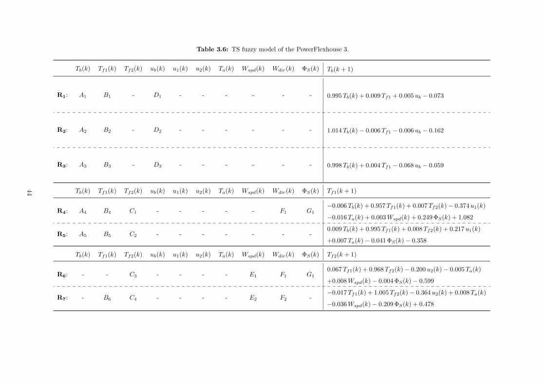
Table 3.6: TS fuzzy model of the PowerFlexhouse 3.
Tb(k) Tf1(k) Tf2(k) ub(k) u1(k) u2(k) Ta(k) Wspd(k) Wdir(k) ΦS(k) Tb(k + 1)
R1: A1 B1 - D1 - - - - - - 0.995Tb(k) + 0.009Tf1 + 0.005ub − 0.073
R2: A2 B2 - D2 - - - - - - 1.014Tb(k)− 0.006Tf1 − 0.006ub − 0.162
R3: A3 B3 - D3 - - - - - - 0.998Tb(k) + 0.004Tf1 − 0.068ub − 0.059
Tb(k) Tf1(k) Tf2(k) ub(k) u1(k) u2(k) Ta(k) Wspd(k) Wdir(k) ΦS(k) Tf1(k + 1)
R4: A4 B4 C1 - - - - - F1 G1
−0.006Tb(k) + 0.957Tf1(k) + 0.007Tf2(k)− 0.374u1(k)
−0.016Ta(k) + 0.003Wspd(k) + 0.249 ΦS(k) + 1.082
R5: A5 B5 C2 - - - - - - -0.009Tb(k) + 0.995Tf1(k) + 0.008Tf2(k) + 0.217u1(k)
+0.007Ta(k)− 0.041 ΦS(k)− 0.358
Tb(k) Tf1(k) Tf2(k) ub(k) u1(k) u2(k) Ta(k) Wspd(k) Wdir(k) ΦS(k) Tf2(k + 1)
R6: - - C3 - - - - E1 F1 G1
0.067Tf1(k) + 0.968Tf2(k)− 0.200u2(k)− 0.005Ta(k)
+0.008Wspd(k)− 0.004 ΦS(k)− 0.599
R7: - B6 C4 - - - - E2 F2 -−0.017Tf1(k) + 1.005Tf2(k)− 0.364u2(k) + 0.008Ta(k)
−0.036Wspd(k)− 0.209 ΦS(k) + 0.478
44
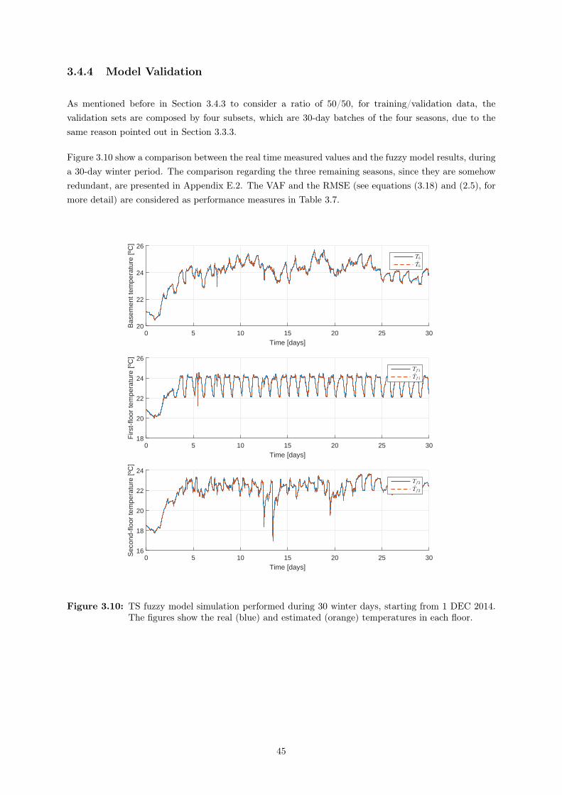
3.4.4 Model Validation
As mentioned before in Section 3.4.3 to consider a ratio of 50/50, for training/validation data, thevalidation sets are composed by four subsets, which are 30-day batches of the four seasons, due to thesame reason pointed out in Section 3.3.3.
Figure 3.10 show a comparison between the real time measured values and the fuzzy model results, duringa 30-day winter period. The comparison regarding the three remaining seasons, since they are somehowredundant, are presented in Appendix E.2. The VAF and the RMSE (see equations (3.18) and (2.5), formore detail) are considered as performance measures in Table 3.7.
0 5 10 15 20 25 30
Time [days]
20
22
24
26
Bas
emen
t tem
pera
ture
[ºC
]
Tb
Tb
0 5 10 15 20 25 30
Time [days]
18
20
22
24
26
Firs
t-flo
or te
mpe
ratu
re [º
C]
Tf1
Tf1
0 5 10 15 20 25 30
Time [days]
16
18
20
22
24
Sec
ond-
floor
tem
pera
ture
[ºC
]
Tf2
Tf2
Figure 3.10: TS fuzzy model simulation performed during 30 winter days, starting from 1 DEC 2014.The figures show the real (blue) and estimated (orange) temperatures in each floor.
45

Table 3.7: Performance assessment of the TS fuzzy model for the 4-season simulation.
Tb Tf1 Tf2
AutumnVAF 99.84 99.77 99.88
RMSE 0.05 0.08 0.05
WinterVAF 99.63 99.15 99.11
RMSE 0.06 0.10 0.11
SpringVAF 99.42 98.75 98.81
RMSE 0.11 0.09 0.15
SummerVAF 99.91 99.78 99.91
RMSE 0.04 0.08 0.05
3.5 Discussion
Comparing Tables 3.3 and 3.7 and Figures 3.6 and 3.10, it is visible that both models shown very highperformances while characterizing and estimating the system behavior. A popular approach is to replacethe real system with the most accurate developed model, like in [21]. In this case, comparing the modeldeveloped in Section 3.3 and the model develop in Section 3.4, the TS fuzzy model is the best performer.
In this thesis, the controllers are going to be developed based on the SDE state-space model and the realsystem will be replaced by the TS fuzzy model. Using this simulation scheme, the performed simulationswill contain the uncertainty regarding model-plant mismatch, which is a characteristic feature of theMPC real-time control experiments. In this way, it is understandable that the performance is going todecrease, when compared to a simulation scheme without model-plant mismatch, although it increasesthe probability of good performance by the controller, in a real world experiment conditions.
46

Chapter 4
Economic Model Predictive Control
In this chapter the controller will be formulated and designed. In Section 4.1 an overview on MPC isgiven. The classical MPC is introduced in Section 4.2. In Section 4.3 the EMPC is formulated andits main differences, comparing it to the classical MPC, are pointed out. In Section 4.4, the inherentoptimization issues are discussed, an EMPC for smart energy systems applications is designed, based onthe models developed in Chapter 3, and its control performance assessment is presented and a methodfor both improving the performance and decrease the computation time is proposed. Section 4.5 endsthe chapter, drawing some important facts, regarding the control simulation results.
4.1 MPC Overview
Since a long time ago, accordingly to [45], the PID control solves in an elegant and satisfactory wayabout 80% of all the control problems in the production industry. In fact, the PID control is to be con-sidered firstly because it doesn’t need an explicitly performed modeling and still guarantee an appreciatedperformance. These represent some of the biggest advantages regarding this type of control.
After the classical control, the work of [28] started a new revolution in the control systems area mostlyknown as modern control. Although the Linear Quadratic Regulator (LQR) and Linear Quadratic Gaus-sian (LQG) controllers are chosen in many control problems, they never had a big impact in the industry.The highly constraint processes, the process nonlinearities and model uncertainties are some well knownreasons for this lack of use.
In order to deal with the remaining 20% industrial control problems, regarding multivariate, coupled-dynamic, constrained, and nonlinear, where the PID controllers lose their efficiency, there is a need toemploy advanced control techniques such as MPC.
Maciejowski [33] stated that "Predictive Control, or Model-Based Predictive Control (’MPC’ or ’MBPC’)as it is sometimes known, is the only advanced control technique – that is, more advanced than standardPID control – to have a significant and widespread impact on industrial process control.".
47
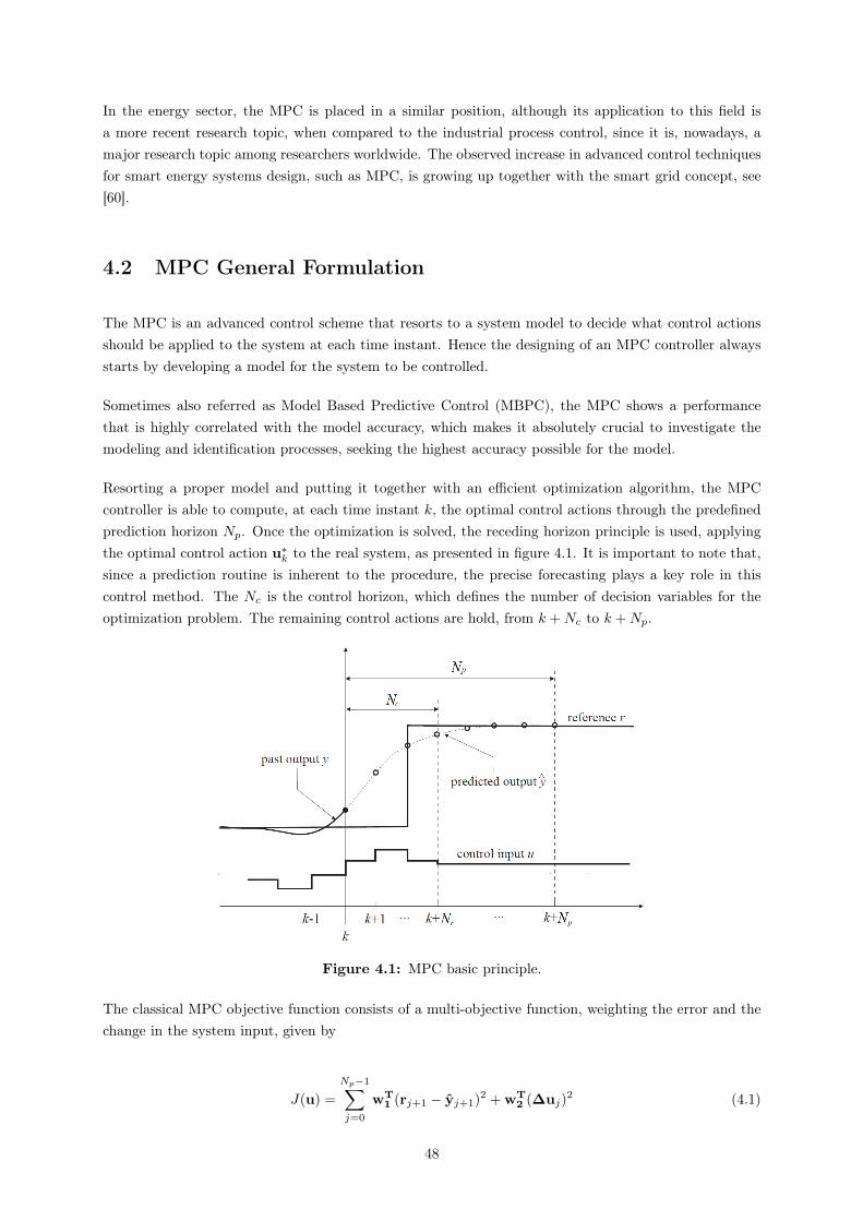
In the energy sector, the MPC is placed in a similar position, although its application to this field isa more recent research topic, when compared to the industrial process control, since it is, nowadays, amajor research topic among researchers worldwide. The observed increase in advanced control techniquesfor smart energy systems design, such as MPC, is growing up together with the smart grid concept, see[60].
4.2 MPC General Formulation
The MPC is an advanced control scheme that resorts to a system model to decide what control actionsshould be applied to the system at each time instant. Hence the designing of an MPC controller alwaysstarts by developing a model for the system to be controlled.
Sometimes also referred as Model Based Predictive Control (MBPC), the MPC shows a performancethat is highly correlated with the model accuracy, which makes it absolutely crucial to investigate themodeling and identification processes, seeking the highest accuracy possible for the model.
Resorting a proper model and putting it together with an efficient optimization algorithm, the MPCcontroller is able to compute, at each time instant k, the optimal control actions through the predefinedprediction horizon Np. Once the optimization is solved, the receding horizon principle is used, applyingthe optimal control action u∗k to the real system, as presented in figure 4.1. It is important to note that,since a prediction routine is inherent to the procedure, the precise forecasting plays a key role in thiscontrol method. The Nc is the control horizon, which defines the number of decision variables for theoptimization problem. The remaining control actions are hold, from k +Nc to k +Np.
Figure 4.1: MPC basic principle.
The classical MPC objective function consists of a multi-objective function, weighting the error and thechange in the system input, given by
J(u) =
Np−1∑j=0
wT1 (rj+1 − yj+1)2 + wT
2 (∆uj)2 (4.1)
48
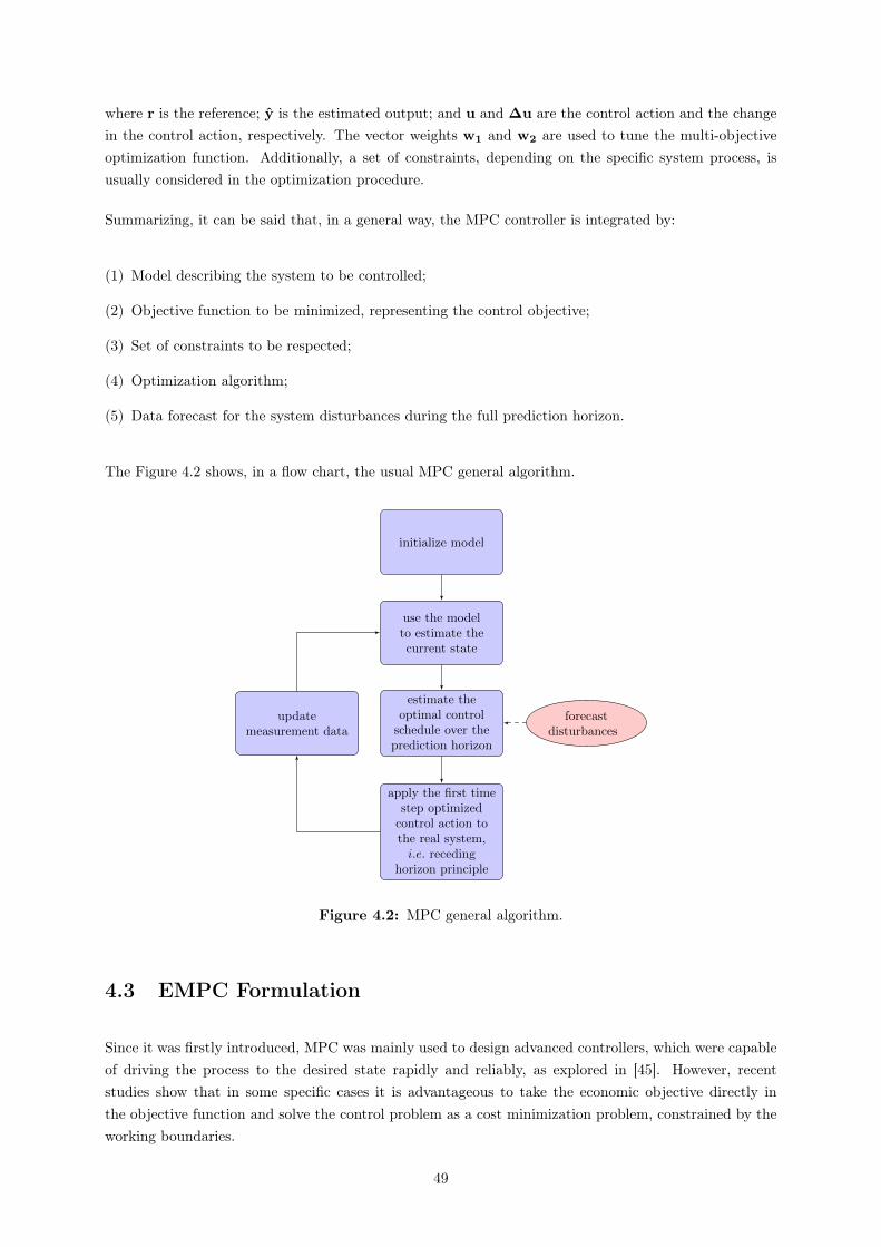
where r is the reference; y is the estimated output; and u and ∆u are the control action and the changein the control action, respectively. The vector weights w1 and w2 are used to tune the multi-objectiveoptimization function. Additionally, a set of constraints, depending on the specific system process, isusually considered in the optimization procedure.
Summarizing, it can be said that, in a general way, the MPC controller is integrated by:
(1) Model describing the system to be controlled;
(2) Objective function to be minimized, representing the control objective;
(3) Set of constraints to be respected;
(4) Optimization algorithm;
(5) Data forecast for the system disturbances during the full prediction horizon.
The Figure 4.2 shows, in a flow chart, the usual MPC general algorithm.
initialize model
use the modelto estimate thecurrent state
estimate theoptimal control
schedule over theprediction horizon
forecastdisturbances
updatemeasurement data
apply the first timestep optimized
control action tothe real system,i.e. receding
horizon principle
Figure 4.2: MPC general algorithm.
4.3 EMPC Formulation
Since it was firstly introduced, MPC was mainly used to design advanced controllers, which were capableof driving the process to the desired state rapidly and reliably, as explored in [45]. However, recentstudies show that in some specific cases it is advantageous to take the economic objective directly inthe objective function and solve the control problem as a cost minimization problem, constrained by theworking boundaries.
49
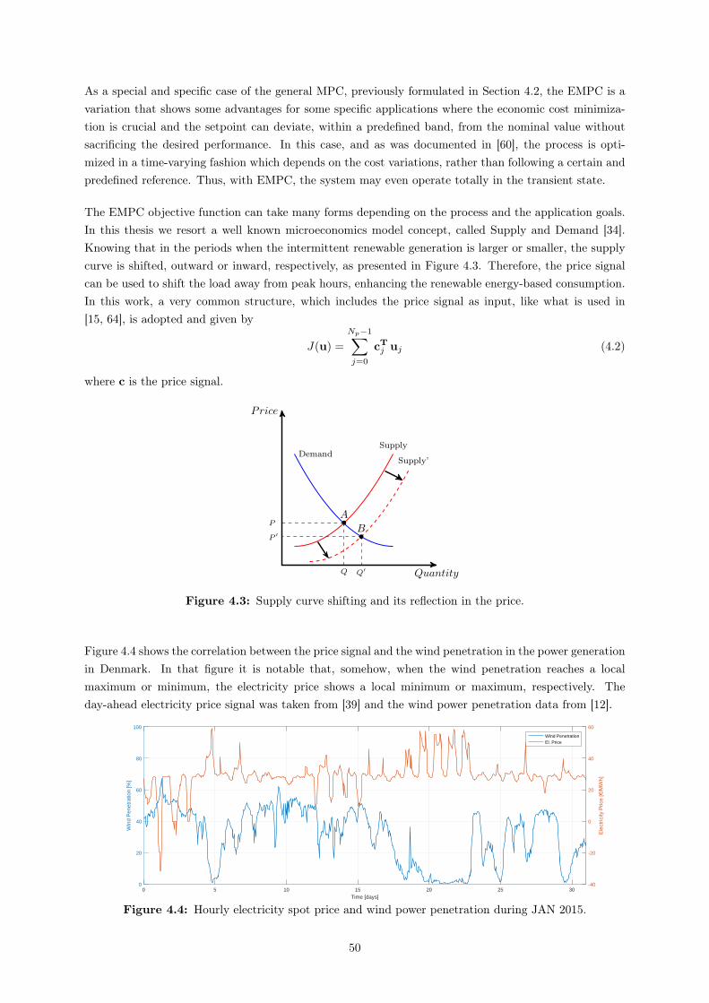
As a special and specific case of the general MPC, previously formulated in Section 4.2, the EMPC is avariation that shows some advantages for some specific applications where the economic cost minimiza-tion is crucial and the setpoint can deviate, within a predefined band, from the nominal value withoutsacrificing the desired performance. In this case, and as was documented in [60], the process is opti-mized in a time-varying fashion which depends on the cost variations, rather than following a certain andpredefined reference. Thus, with EMPC, the system may even operate totally in the transient state.
The EMPC objective function can take many forms depending on the process and the application goals.In this thesis we resort a well known microeconomics model concept, called Supply and Demand [34].Knowing that in the periods when the intermittent renewable generation is larger or smaller, the supplycurve is shifted, outward or inward, respectively, as presented in Figure 4.3. Therefore, the price signalcan be used to shift the load away from peak hours, enhancing the renewable energy-based consumption.In this work, a very common structure, which includes the price signal as input, like what is used in[15, 64], is adopted and given by
J(u) =
Np−1∑j=0
cTj uj (4.2)
where c is the price signal.
Quantity
Price
SupplyDemand
A
Supply’
B
Q′
P ′
Q
P
Figure 4.3: Supply curve shifting and its reflection in the price.
Figure 4.4 shows the correlation between the price signal and the wind penetration in the power generationin Denmark. In that figure it is notable that, somehow, when the wind penetration reaches a localmaximum or minimum, the electricity price shows a local minimum or maximum, respectively. Theday-ahead electricity price signal was taken from [39] and the wind power penetration data from [12].
0 5 10 15 20 25 30
Time [days]
0
20
40
60
80
100
Win
d P
enet
ratio
n [%
]
-40
-20
0
20
40
60
Wind PenetrationEl. Price
Figure 4.4: Hourly electricity spot price and wind power penetration during JAN 2015.
50

Table 4.1 represents a general comparison between MPC and EMPC, including their principal features.
Table 4.1: Traditional MPC vs EMPC.
Traditional MPC EMPC
Steady-State Operation Time-Varying Operation
Operation Cost as Constraint Function Operation Cost as Objective Function
Setpoint Tracking as Objective Function Setpoint boundary as Constraint Function
4.4 EMPC Design
4.4.1 The Optimization Algorithm
The EMPC is a variant of the classical MPC, which has been successfully applied to particular cases,such as [15, 19, 30, 42, 64]. The capability of exploring the flexibility in the Distributed Energy Resources(DER), shifting the load away from the peak hours, justifies the special attention that is being paid tothis type of controller, which is being applied to a wide range of smart energy systems applications. It isa control philosophy based on a very intuitive principle, where the control problem is interpreted as anoptimization problem and lies in the choice of the best control actions at each time instant, considering aset of relevant information (such as the system model, the objective function, the disturbances forecastsand the set of operational constraints).
Thus, the EMPC optimization problem needs to be solved, at each time instant, through the predefinedprediction horizon Np. Once solved, the receding horizon principle is used, applying the optimal controlaction u∗0 to the system. Generally, this problem can be defined as follows:
u∗k = argmin JE =
Np−1∑k=0
cTk uk (4.3a)
subject to
umin ≤ uk ≤ umax, k = 0, . . . , Np − 1 (4.3b)
∆umin ≤∆uk ≤∆umax, k = 0, . . . , Np − 1 (4.3c)
ymin ≤ yk ≤ ymax, k = 1, . . . , Np (4.3d)
where ck is the electricity cost vector; uk is the input vector; and yk is the output vector.
In Figure 4.5, the general algorithm for the EMPC problem solving, in a block diagram, is presented.
51
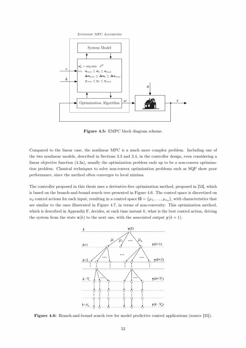
Optimization Algorithmu∗ y
System Model
u∗k = argmin JE
s.t. umin ≤ uk ≤ umax
∆umin ≤∆uk ≤∆umax
ymin ≤ yk ≤ ymax
c
d
d
•
Economic MPC Algorithm
Figure 4.5: EMPC block diagram scheme.
Compared to the linear case, the nonlinear MPC is a much more complex problem. Including one ofthe two nonlinear models, described in Sections 3.3 and 3.4, in the controller design, even considering alinear objective function (4.3a), usually the optimization problem ends up to be a non-convex optimiza-tion problem. Classical techniques to solve non-convex optimization problems such as SQP show poorperformance, since the method often converges to local minima.
The controller proposed in this thesis uses a derivative-free optimization method, proposed in [53], whichis based on the branch-and-bound search tree presented in Figure 4.6. The control space is discretized onnd control actions for each input, resulting in a control space Ω = µ1, . . . , µnd
, with characteristics thatare similar to the ones illustrated in Figure 4.7, in terms of non-convexity. This optimization method,which is described in Appendix F, decides, at each time instant k, what is the best control action, drivingthe system from the state x(k) to the next one, with the associated output y(k + 1).
Figure 4.6: Branch-and-bound search tree for model predictive control applications (source [35]).
52
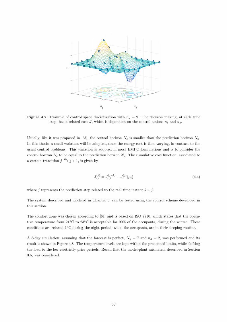
J
u2u
1
Figure 4.7: Example of control space discretization with nd = 9. The decision making, at each timestep, has a related cost J , which is dependent on the control actions u1 and u2.
Usually, like it was proposed in [53], the control horizon Nc is smaller than the prediction horizon Np.In this thesis, a small variation will be adopted, since the energy cost is time-varying, in contrast to theusual control problems. This variation is adopted in most EMPC formulations and is to consider thecontrol horizon Nc to be equal to the prediction horizon Np. The cumulative cost function, associated toa certain transition j µi−→ j + 1, is given by
J(j)c,i = J
(j−1)c,i + J
(j)i (µi) (4.4)
where j represents the prediction step related to the real time instant k + j.
The system described and modeled in Chapter 3, can be tested using the control scheme developed inthis section.
The comfort zone was chosen according to [61] and is based on ISO 7730, which states that the opera-tive temperature from 21C to 23C is acceptable for 90% of the occupants, during the winter. Theseconditions are relaxed 1C during the night period, when the occupants, are in their sleeping routine.
A 5-day simulation, assuming that the forecast is perfect, Np = 7 and nd = 2, was performed and itsresult is shown in Figure 4.8. The temperature levels are kept within the predefined limits, while shiftingthe load to the low electricity price periods. Recall that the model-plant mismatch, described in Section3.5, was considered.
53
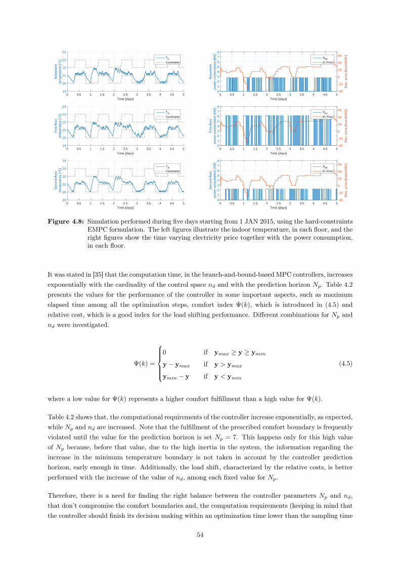
0 0.5 1 1.5 2 2.5 3 3.5 4 4.5 5
Time [days]
19
20
21
22
23
24B
asem
ent
tem
pera
ture
[°C
]T
b
Constraints
0 0.5 1 1.5 2 2.5 3 3.5 4 4.5 5
Time [days]
19
20
21
22
23
24
Firs
t-flo
orte
mpe
ratu
re [°
C]
Tf1
Constraints
0 0.5 1 1.5 2 2.5 3 3.5 4 4.5 5
Time [days]
19
20
21
22
23
24
Sec
ond-
floor
tem
pera
ture
[°C
]
Tf2
Constraints
0 0.5 1 1.5 2 2.5 3 3.5 4 4.5 5
Time [days]
0
1
2
3
4
5
6
7
8
Bas
emen
tpo
wer
con
sum
ptio
n [k
W]
-40
-20
0
20
40
60Φ
Hb
El. Price
0 0.5 1 1.5 2 2.5 3 3.5 4 4.5 5
Time [days]
0
1
2
3
4
5
6
7
8
Firs
t-flo
orpo
wer
con
sum
ptio
n [k
W]
-40
-20
0
20
40
60Φ
H1
El. Price
0 0.5 1 1.5 2 2.5 3 3.5 4 4.5 5
Time [days]
0
1
2
3
4
5
6
7
8
Sec
ond-
floor
pow
er c
onsu
mpt
ion
[kW
]
-40
-20
0
20
40
60Φ
H2
El. Price
Figure 4.8: Simulation performed during five days starting from 1 JAN 2015, using the hard-constraintsEMPC formulation. The left figures illustrate the indoor temperature, in each floor, and theright figures show the time varying electricity price together with the power consumption,in each floor.
It was stated in [35] that the computation time, in the branch-and-bound-based MPC controllers, increasesexponentially with the cardinality of the control space nd and with the prediction horizon Np. Table 4.2presents the values for the performance of the controller in some important aspects, such as maximumelapsed time among all the optimization steps, comfort index Ψ(k), which is introduced in (4.5) andrelative cost, which is a good index for the load shifting performance. Different combinations for Np andnd were investigated.
Ψ(k) =
0 if ymax ≥ y ≥ ymin
y − ymax if y > ymax
ymin − y if y < ymin
(4.5)
where a low value for Ψ(k) represents a higher comfort fulfillment than a high value for Ψ(k).
Table 4.2 shows that, the computational requirements of the controller increase exponentially, as expected,while Np and nd are increased. Note that the fulfillment of the prescribed comfort boundary is frequentlyviolated until the value for the prediction horizon is set Np = 7. This happens only for this high valueof Np because, before that value, due to the high inertia in the system, the information regarding theincrease in the minimum temperature boundary is not taken in account by the controller predictionhorizon, early enough in time. Additionally, the load shift, characterized by the relative costs, is betterperformed with the increase of the value of nd, among each fixed value for Np.
Therefore, there is a need for finding the right balance between the controller parameters Np and nd,that don’t compromise the comfort boundaries and, the computation requirements (keeping in mind thatthe controller should finish its decision making within an optimization time lower than the sampling time
54
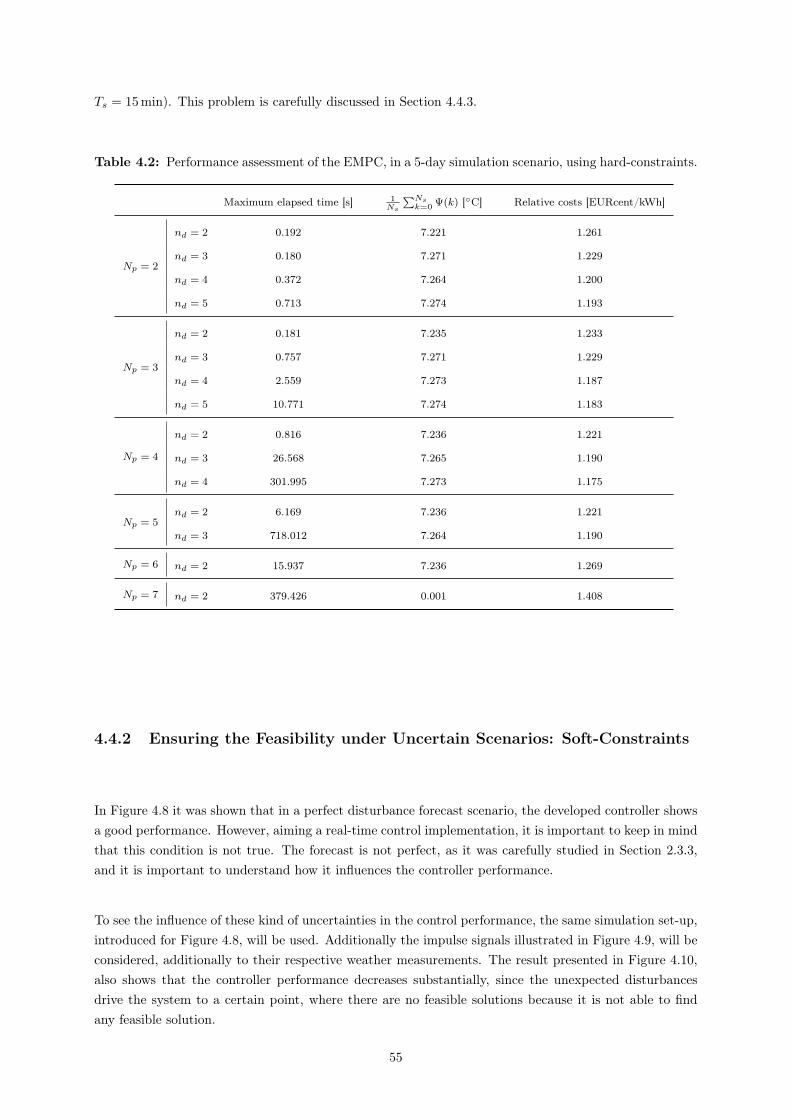
Ts = 15min). This problem is carefully discussed in Section 4.4.3.
Table 4.2: Performance assessment of the EMPC, in a 5-day simulation scenario, using hard-constraints.
Maximum elapsed time [s] 1Ns
∑Nsk=0 Ψ(k) [C] Relative costs [EURcent/kWh]
Np = 2
nd = 2 0.192 7.221 1.261
nd = 3 0.180 7.271 1.229
nd = 4 0.372 7.264 1.200
nd = 5 0.713 7.274 1.193
Np = 3
nd = 2 0.181 7.235 1.233
nd = 3 0.757 7.271 1.229
nd = 4 2.559 7.273 1.187
nd = 5 10.771 7.274 1.183
Np = 4
nd = 2 0.816 7.236 1.221
nd = 3 26.568 7.265 1.190
nd = 4 301.995 7.273 1.175
Np = 5nd = 2 6.169 7.236 1.221
nd = 3 718.012 7.264 1.190
Np = 6 nd = 2 15.937 7.236 1.269
Np = 7 nd = 2 379.426 0.001 1.408
4.4.2 Ensuring the Feasibility under Uncertain Scenarios: Soft-Constraints
In Figure 4.8 it was shown that in a perfect disturbance forecast scenario, the developed controller showsa good performance. However, aiming a real-time control implementation, it is important to keep in mindthat this condition is not true. The forecast is not perfect, as it was carefully studied in Section 2.3.3,and it is important to understand how it influences the controller performance.
To see the influence of these kind of uncertainties in the control performance, the same simulation set-up,introduced for Figure 4.8, will be used. Additionally the impulse signals illustrated in Figure 4.9, will beconsidered, additionally to their respective weather measurements. The result presented in Figure 4.10,also shows that the controller performance decreases substantially, since the unexpected disturbancesdrive the system to a certain point, where there are no feasible solutions because it is not able to findany feasible solution.
55
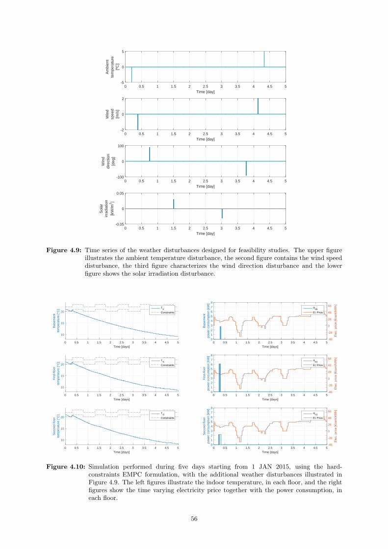
0 0.5 1 1.5 2 2.5 3 3.5 4 4.5 5
Time [day]
-5
0
5
Am
bien
tte
mpe
ratu
re[º
C]
0 0.5 1 1.5 2 2.5 3 3.5 4 4.5 5
Time [day]
-2
0
2
Win
dsp
eed
[m/s
]
0 0.5 1 1.5 2 2.5 3 3.5 4 4.5 5
Time [day]
-100
0
100
Win
ddi
rect
ion
[deg
]
0 0.5 1 1.5 2 2.5 3 3.5 4 4.5 5
Time [day]
-0.05
0
0.05
Sol
arirr
adia
tion
[kW
/m2]
Figure 4.9: Time series of the weather disturbances designed for feasibility studies. The upper figureillustrates the ambient temperature disturbance, the second figure contains the wind speeddisturbance, the third figure characterizes the wind direction disturbance and the lowerfigure shows the solar irradiation disturbance.
0 0.5 1 1.5 2 2.5 3 3.5 4 4.5 5
Time [days]
10
15
20
Bas
emen
tte
mpe
ratu
re [°
C] T
b
Constraints
0 0.5 1 1.5 2 2.5 3 3.5 4 4.5 5
Time [days]
10
15
20
Firs
t-flo
orte
mpe
ratu
re [°
C] T
f1
Constraints
0 0.5 1 1.5 2 2.5 3 3.5 4 4.5 5
Time [days]
10
15
20
Sec
ond-
floor
tem
pera
ture
[°C
] Tf2
Constraints
0 0.5 1 1.5 2 2.5 3 3.5 4 4.5 5
Time [days]
0
1
2
3
4
5
6
7
8
Bas
emen
tpo
wer
con
sum
ptio
n [k
W]
-40
-20
0
20
40
60Φ
Hb
El. Price
0 0.5 1 1.5 2 2.5 3 3.5 4 4.5 5
Time [days]
0
1
2
3
4
5
6
7
8
Firs
t-flo
orpo
wer
con
sum
ptio
n [k
W]
-40
-20
0
20
40
60Φ
H1
El. Price
0 0.5 1 1.5 2 2.5 3 3.5 4 4.5 5
Time [days]
0
1
2
3
4
5
6
7
8
Sec
ond-
floor
pow
er c
onsu
mpt
ion
[kW
]
-40
-20
0
20
40
60Φ
H2
El. Price
Figure 4.10: Simulation performed during five days starting from 1 JAN 2015, using the hard-constraints EMPC formulation, with the additional weather disturbances illustrated inFigure 4.9. The left figures illustrate the indoor temperature, in each floor, and the rightfigures show the time varying electricity price together with the power consumption, ineach floor.
56

To ensure the feasibility of the optimization problem, instead of using the hard-constraints defined in theformulation (4.3), soft-constraints will be added to the EMPC algorithm and included in the optimizationproblem shown in equations (4.6).
u∗k = argmin JE =
Np−1∑k=0
cTk uk +
Np∑k=1
ρv vk (4.6a)
subject to
umin ≤ uk ≤ umax, k = 0, . . . , Np − 1 (4.6b)
∆umin ≤∆uk ≤∆umax, k = 0, . . . , Np − 1 (4.6c)
ymin ≤ yk + vk, k = 1, . . . , Np (4.6d)
ymax ≥ yk − vk, k = 1, . . . , Np (4.6e)
vk ≥ 0, k = 1, . . . , Np. (4.6f)
The slack variable vk is introduced, together with an associated penalty cost ρv, to ensure that theoptimization always finds feasible solutions. The value for ρv is usually chosen to be high, so that therelaxed optimization problem will have an optimal solution with vk = 0, if possible. Therefore it assuredthat the controller will try to respect the boundaries ymin and ymax. At the same time, if a certainuncertainty or disturbance causes the infeasibility of the optimization problem, the slack variable is usedto ”enlarge” the feasible region and obtain a feasible solution.
The same scenario that was presented for the Figure 4.10 simulation, will be used to investigate theperformance of the EMPC controller, with the soft-constraints formulation introduced in (4.6). Figure4.11 presents the results and, according to them, it can be concluded that the controller will always findfeasible solutions, even considering disturbances and forecast uncertainties. Note that even choosing thedisturbances to be high enough, the performance has shown to be very satisfactory, mostly due to thereceding horizon characteristics of the MPC algorithm.
From now on, the perfect forecast scenario will not be considered anymore, since the type of soft-constraintEMPC, developed in this section, is able to deal with this kind of uncertainties.
57
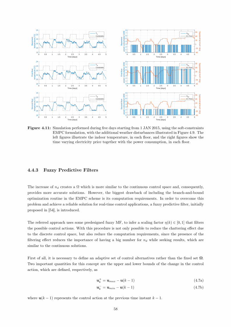
0 0.5 1 1.5 2 2.5 3 3.5 4 4.5 5
Time [days]
19
20
21
22
23
24B
asem
ent
tem
pera
ture
[°C
] Tb
Constraints
0 0.5 1 1.5 2 2.5 3 3.5 4 4.5 5
Time [days]
19
20
21
22
23
24
Firs
t-flo
orte
mpe
ratu
re [°
C] T
f1
Constraints
0 0.5 1 1.5 2 2.5 3 3.5 4 4.5 5
Time [days]
19
20
21
22
23
24
Sec
ond-
floor
tem
pera
ture
[°C
] Tf2
Constraints
0 0.5 1 1.5 2 2.5 3 3.5 4 4.5 5
Time [days]
0
1
2
3
4
5
6
7
8
Bas
emen
tpo
wer
con
sum
ptio
n [k
W]
-40
-20
0
20
40
60Φ
Hb
El. Price
0 0.5 1 1.5 2 2.5 3 3.5 4 4.5 5
Time [days]
0
1
2
3
4
5
6
7
8
Firs
t-flo
orpo
wer
con
sum
ptio
n [k
W]
-40
-20
0
20
40
60Φ
H1
El. Price
0 0.5 1 1.5 2 2.5 3 3.5 4 4.5 5
Time [days]
0
1
2
3
4
5
6
7
8
Sec
ond-
floor
pow
er c
onsu
mpt
ion
[kW
]
-40
-20
0
20
40
60Φ
H2
El. Price
Figure 4.11: Simulation performed during five days starting from 1 JAN 2015, using the soft-constraintsEMPC formulation, with the additional weather disturbances illustrated in Figure 4.9. Theleft figures illustrate the indoor temperature, in each floor, and the right figures show thetime varying electricity price together with the power consumption, in each floor.
4.4.3 Fuzzy Predictive Filters
The increase of nd creates a Ω which is more similar to the continuous control space and, consequently,provides more accurate solutions. However, the biggest drawback of including the branch-and-boundoptimization routine in the EMPC scheme is its computation requirements. In order to overcome thisproblem and achieve a reliable solution for real-time control applications, a fuzzy predictive filter, initiallyproposed in [54], is introduced.
The referred approach uses some predesigned fuzzy MF, to infer a scaling factor η(k) ∈ [0, 1] that filtersthe possible control actions. With this procedure is not only possible to reduce the chattering effect dueto the discrete control space, but also reduce the computation requirements, since the presence of thefiltering effect reduces the importance of having a big number for nd while seeking results, which aresimilar to the continuous solutions.
First of all, it is necessary to define an adaptive set of control alternatives rather than the fixed set Ω.Two important quantities for this concept are the upper and lower bounds of the change in the controlaction, which are defined, respectively, as
u+k = umax − u(k − 1) (4.7a)
u−k = umin − u(k − 1) (4.7b)
where u(k − 1) represents the control action at the previous time instant k − 1.
58
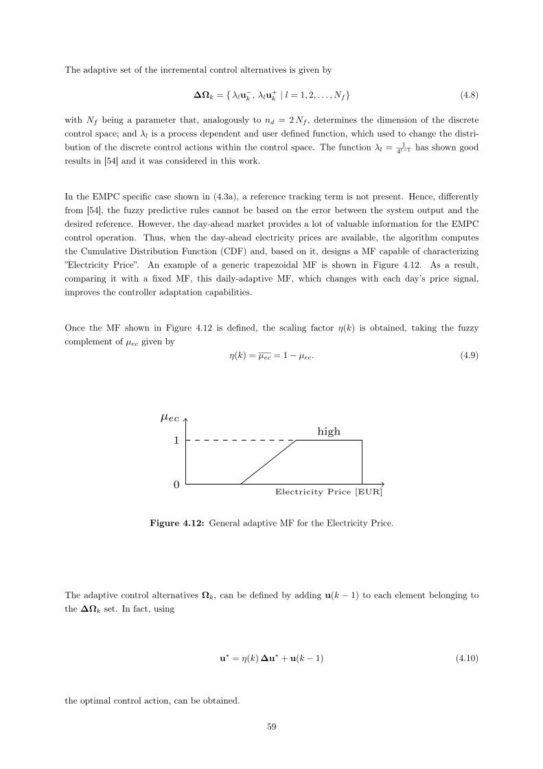
The adaptive set of the incremental control alternatives is given by
∆Ωk = λlu−k , λlu+k | l = 1, 2, . . . , Nf (4.8)
with Nf being a parameter that, analogously to nd = 2Nf , determines the dimension of the discretecontrol space; and λl is a process dependent and user defined function, which used to change the distri-bution of the discrete control actions within the control space. The function λl = 1
4l−1 has shown goodresults in [54] and it was considered in this work.
In the EMPC specific case shown in (4.3a), a reference tracking term is not present. Hence, differentlyfrom [54], the fuzzy predictive rules cannot be based on the error between the system output and thedesired reference. However, the day-ahead market provides a lot of valuable information for the EMPCcontrol operation. Thus, when the day-ahead electricity prices are available, the algorithm computesthe Cumulative Distribution Function (CDF) and, based on it, designs a MF capable of characterizing”Electricity Price”. An example of a generic trapezoidal MF is shown in Figure 4.12. As a result,comparing it with a fixed MF, this daily-adaptive MF, which changes with each day’s price signal,improves the controller adaptation capabilities.
Once the MF shown in Figure 4.12 is defined, the scaling factor η(k) is obtained, taking the fuzzycomplement of µec given by
η(k) = µec = 1− µec. (4.9)
Electricity Price [EUR]
µec
0
1high
Figure 4.12: General adaptive MF for the Electricity Price.
The adaptive control alternatives Ωk, can be defined by adding u(k − 1) to each element belonging tothe ∆Ωk set. In fact, using
u∗ = η(k) ∆u∗ + u(k − 1) (4.10)
the optimal control action, can be obtained.
59
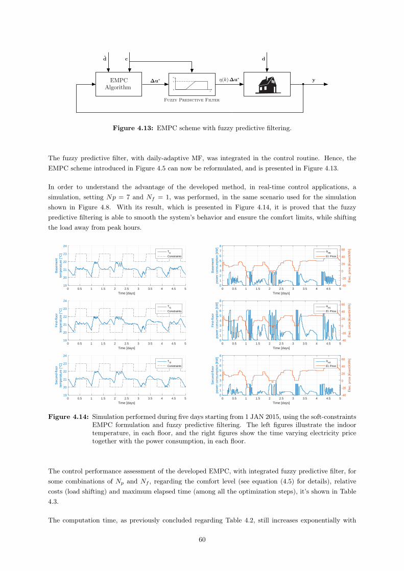
EMPCAlgorithm
c
µ
0
1∆u∗ η(k)∆u∗ y
cd d
•
Fuzzy Predictive Filter
Figure 4.13: EMPC scheme with fuzzy predictive filtering.
The fuzzy predictive filter, with daily-adaptive MF, was integrated in the control routine. Hence, theEMPC scheme introduced in Figure 4.5 can now be reformulated, and is presented in Figure 4.13.
In order to understand the advantage of the developed method, in real-time control applications, asimulation, setting Np = 7 and Nf = 1, was performed, in the same scenario used for the simulationshown in Figure 4.8. With its result, which is presented in Figure 4.14, it is proved that the fuzzypredictive filtering is able to smooth the system’s behavior and ensure the comfort limits, while shiftingthe load away from peak hours.
0 0.5 1 1.5 2 2.5 3 3.5 4 4.5 5
Time [days]
19
20
21
22
23
24
Bas
emen
tte
mpe
ratu
re [°
C]
Tb
Constraints
0 0.5 1 1.5 2 2.5 3 3.5 4 4.5 5
Time [days]
19
20
21
22
23
24
Firs
t-flo
orte
mpe
ratu
re [°
C]
Tf1
Constraints
0 0.5 1 1.5 2 2.5 3 3.5 4 4.5 5
Time [days]
19
20
21
22
23
24
Sec
ond-
floor
tem
pera
ture
[°C
]
Tf2
Constraints
0 0.5 1 1.5 2 2.5 3 3.5 4 4.5 5
Time [days]
0
1
2
3
4
5
6
7
8
Bas
emen
tpo
wer
con
sum
ptio
n [k
W]
-40
-20
0
20
40
60Φ
Hb
El. Price
0 0.5 1 1.5 2 2.5 3 3.5 4 4.5 5
Time [days]
0
1
2
3
4
5
6
7
8
Firs
t-flo
orpo
wer
con
sum
ptio
n [k
W]
-40
-20
0
20
40
60Φ
H1
El. Price
0 0.5 1 1.5 2 2.5 3 3.5 4 4.5 5
Time [days]
0
1
2
3
4
5
6
7
8
Sec
ond-
floor
pow
er c
onsu
mpt
ion
[kW
]
-40
-20
0
20
40
60Φ
H2
El. Price
Figure 4.14: Simulation performed during five days starting from 1 JAN 2015, using the soft-constraintsEMPC formulation and fuzzy predictive filtering. The left figures illustrate the indoortemperature, in each floor, and the right figures show the time varying electricity pricetogether with the power consumption, in each floor.
The control performance assessment of the developed EMPC, with integrated fuzzy predictive filter, forsome combinations of Np and Nf , regarding the comfort level (see equation (4.5) for details), relativecosts (load shifting) and maximum elapsed time (among all the optimization steps), it’s shown in Table4.3.
The computation time, as previously concluded regarding Table 4.2, still increases exponentially with
60
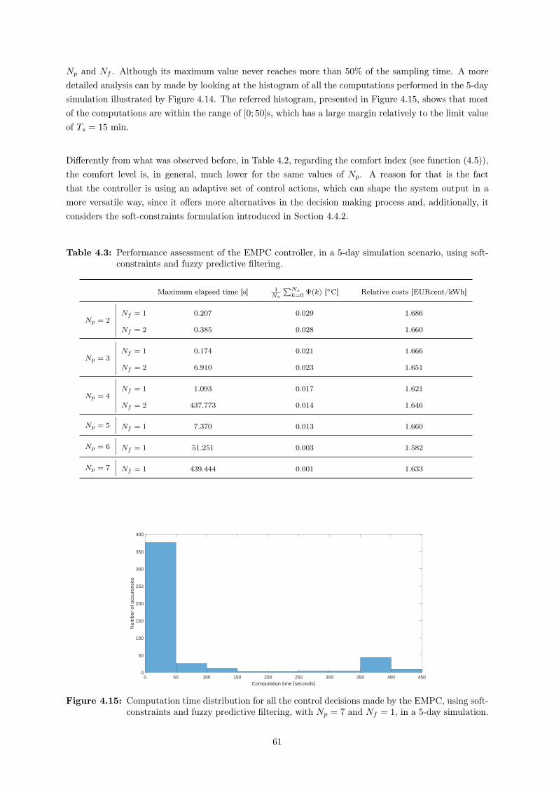
Np and Nf . Although its maximum value never reaches more than 50% of the sampling time. A moredetailed analysis can by made by looking at the histogram of all the computations performed in the 5-daysimulation illustrated by Figure 4.14. The referred histogram, presented in Figure 4.15, shows that mostof the computations are within the range of [0; 50]s, which has a large margin relatively to the limit valueof Ts = 15 min.
Differently from what was observed before, in Table 4.2, regarding the comfort index (see function (4.5)),the comfort level is, in general, much lower for the same values of Np. A reason for that is the factthat the controller is using an adaptive set of control actions, which can shape the system output in amore versatile way, since it offers more alternatives in the decision making process and, additionally, itconsiders the soft-constraints formulation introduced in Section 4.4.2.
Table 4.3: Performance assessment of the EMPC controller, in a 5-day simulation scenario, using soft-constraints and fuzzy predictive filtering.
Maximum elapsed time [s] 1Ns
∑Nsk=0 Ψ(k) [C] Relative costs [EURcent/kWh]
Np = 2Nf = 1 0.207 0.029 1.686
Nf = 2 0.385 0.028 1.660
Np = 3Nf = 1 0.174 0.021 1.666
Nf = 2 6.910 0.023 1.651
Np = 4Nf = 1 1.093 0.017 1.621
Nf = 2 437.773 0.014 1.646
Np = 5 Nf = 1 7.370 0.013 1.660
Np = 6 Nf = 1 51.251 0.003 1.582
Np = 7 Nf = 1 439.444 0.001 1.633
0 50 100 150 200 250 300 350 400 450Computation time [seconds]
0
50
100
150
200
250
300
350
400
Num
ber
of o
ccur
ence
s
Figure 4.15: Computation time distribution for all the control decisions made by the EMPC, using soft-constraints and fuzzy predictive filtering, with Np = 7 and Nf = 1, in a 5-day simulation.
61

4.5 Discussion
After the development of the EMPC through the sections of this chapter, it was proved that the controllershows a good performance, while performing the assign task.
The soft-constraint formulation, introduced in Section 4.4.2, improves the controller robustness againstany kind of uncertainties. Therefore, it is a must to the nonlinear EMPC proposed, in this thesis.
Comparing both Table 4.2 and Table 4.15, it is visible that the fuzzy predictive filtering is able to increasethe performance of the EMPC. Specifically, the temperature boundary fulfillment increases for a smallervalue of Np and for a smaller cardinality of the control space nd = 2Nf . Consequently, the shorternumber of control alternatives, at each step, reduces the related computation time, achieving a similarcontrol performance.
Figure 4.14 shows that the load shifting is much higher than the case presented in Figure 4.11, since theenergy consumption trend during peak hours, is much lower. Additionally, the chattering effect, duringperiods when the price signal is higher and the goal is to keep the temperature as close to the minimumtemperature boundary as possible, i.e. aiming a local energy consumption decrease, is also reduced.
In conclusion, the formulation showing the best balance between computational demand, comfort fulfill-ment, and energy shifting (characterized by the relative costs) was the soft-constraint formulation, withfuzzy predictive filtering and the parameters Np = 6 and Nf = 1.
62

Chapter 5
Coupling Electricity and Heating via
Heat Pump Integration
In this chapter the advantages and disadvantages of coupling electricity and heating systems are explored.Section 5.1 starts by giving a general overview on multi-energy systems. Sections 5.2 and Section 5.3describe the modeling procedure of a heat pump and a hot water tank, respectively and explain how theycan be integrated with the building system introduced in Chapter 3. The energetic assessment of thedeveloped solution is explored in Section 5.5. Finally, Section 5.6 presents some important conclusionsregarding the results presented in Section 5.5.
5.1 Multi-Energy Systems Overview
In Section 1.1.1, the state of today’s energetic scenario was presented. In fact, it was shown that isextremely important to accelerate the transition to a fully decarbonized energy system.
Specifically, in this thesis, problems mainly connected to the power system were addressed. However,studies like [31, 32] shown that, aiming to reduce the carbon footprint in the world, there are advantagestreating the different types of energy subsystems, not independently, but as integrated systems. This isthe reason why the so called multi-energy systems are starting to be highly explored, by energy systemsdevelopers, operators and owners.
Combined Heat and Power (CHP) units, heat pumps, electric boilers and so forth, present multipleadvantages and are able to both reduce operation costs and increase the overall efficiency, of the energysystems.
In this chapter a heat pump solution is proposed. Its performance assessment is presented and comparedto the best performing solution, highlighted in Chapter 4.
63
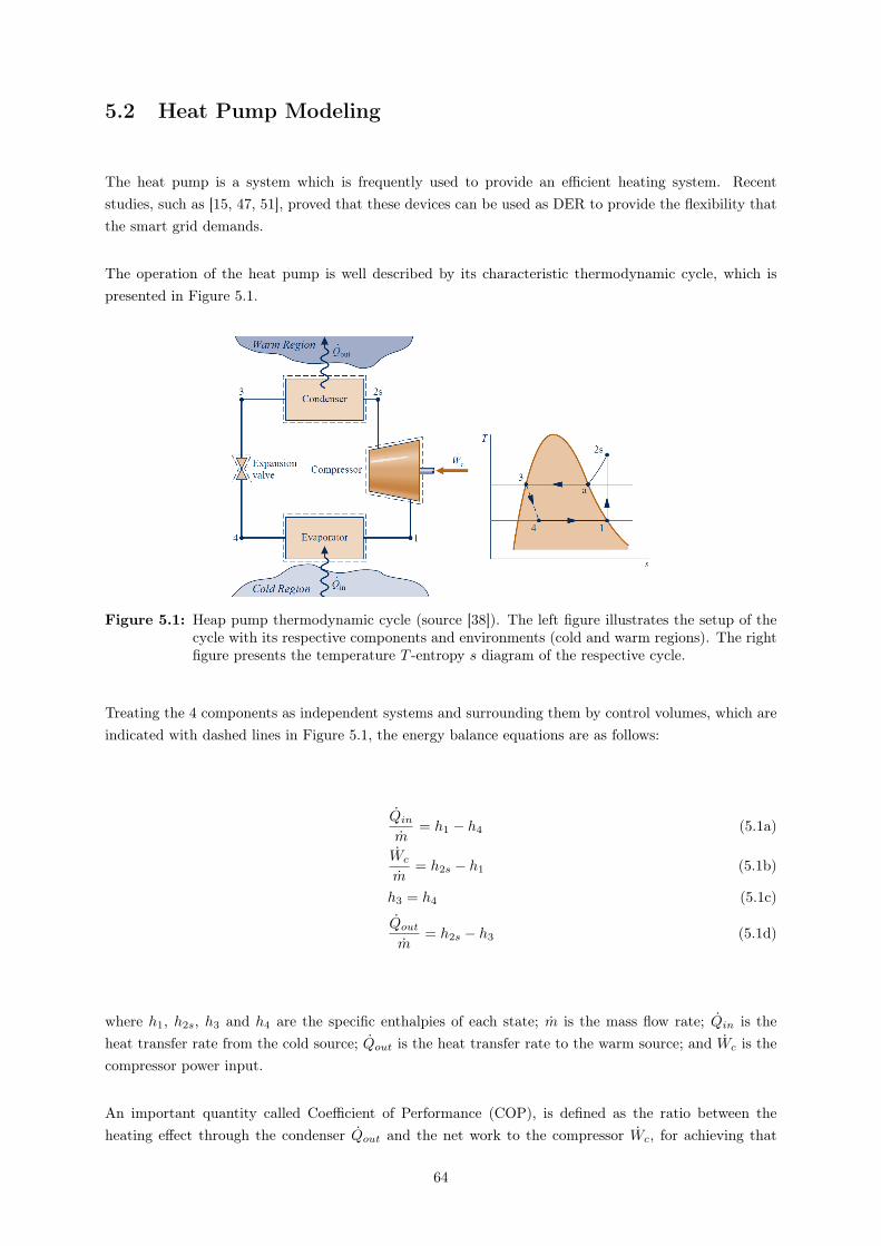
5.2 Heat Pump Modeling
The heat pump is a system which is frequently used to provide an efficient heating system. Recentstudies, such as [15, 47, 51], proved that these devices can be used as DER to provide the flexibility thatthe smart grid demands.
The operation of the heat pump is well described by its characteristic thermodynamic cycle, which ispresented in Figure 5.1.
Figure 5.1: Heap pump thermodynamic cycle (source [38]). The left figure illustrates the setup of thecycle with its respective components and environments (cold and warm regions). The rightfigure presents the temperature T -entropy s diagram of the respective cycle.
Treating the 4 components as independent systems and surrounding them by control volumes, which areindicated with dashed lines in Figure 5.1, the energy balance equations are as follows:
Qinm
= h1 − h4 (5.1a)
Wc
m= h2s − h1 (5.1b)
h3 = h4 (5.1c)
Qoutm
= h2s − h3 (5.1d)
where h1, h2s, h3 and h4 are the specific enthalpies of each state; m is the mass flow rate; Qin is theheat transfer rate from the cold source; Qout is the heat transfer rate to the warm source; and Wc is thecompressor power input.
An important quantity called Coefficient of Performance (COP), is defined as the ratio between theheating effect through the condenser Qout and the net work to the compressor Wc, for achieving that
64

effect. This ratio can be described as
COP =Qout/m
Wc/m(5.2)
which means that
Qout = COP · Wc. (5.3)
The COP is a function of the four states of the heat pump cycle described in Figure 5.1. Consequently,it is possible to estimate a correlation for the COP, depending on the values for the temperatures in thecold and warm regions. However, for control purposes, a commonly applied approach is to assume thatthe COP has a constant and typical value, as proposed in [15].
In this work, the considered heat pump (Type: AWB-AC 201.C13) specifications are presented in Ap-pendix G and they correspond to the heat pump that is installed in the substation, near the buildingintroduced in Section 3.2. Hence, and according to the specifications sheet, the value of COP = 3.70 anda maximum value for the compressor power of Wmax
c = 2.45 kW, are considered for this model.
5.3 Water Tank Modeling
The system described in the previous section already provides, by itself, an increase in flexibility, takingadvantage of the building thermal mass, while operating the heat pump. Nevertheless, to couple it witha hot water tank, increasing the heat storage capability would provide even more flexibility. To studythis phenomenon, a model, representing the thermal dynamics of the referred tank, is needed, see Figure5.2.
water supply
hot water for heating
QHP
Qloss
Tw
Cw
Figure 5.2: Water tank thermal dynamics scheme.
65
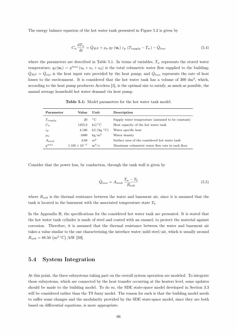
The energy balance equation of the hot water tank presented in Figure 5.2 is given by
CwdTwdt
= QHP + ρw qT (ut) cp (Tsupply − Tw)− Qloss (5.4)
where the parameters are described in Table 5.1. In terms of variables, Tw represents the stored watertemperature; qT (ut) = qmax (ub + u1 + u2) is the total volumetric water flow supplied to the building;QHP = Qout is the heat input rate provided by the heat pump; and Qloss represents the rate of heatlosses to the environment. It is considered that the hot water tank has a volume of 300 dm3, which,according to the heat pump producers Accelera [1], is the optimal size to satisfy, as much as possible, theannual average household hot water demand via heat pump.
Table 5.1: Model parameters for the hot water tank model.
Parameter Value Unit Description
Tsupply 20 C Supply water temperature (assumed to be constant)
Cw 1255.8 kJ/C Heat capacity of the hot water tank
cp 4.186 kJ/(kg C) Water specific heat
ρw 1000 kg/m3 Water density
Atank 2.69 m2 Surface area of the considered hot water tank
qmax 1.105 × 10⁻⁵ m3/s Maximum volumetric water flow rate in each floor
Consider that the power loss, by conduction, through the tank wall is given by
Qloss = AtankTw − TbRwtb
(5.5)
where Rwtb is the thermal resistance between the water and basement air, since it is assumed that thetank is located in the basement with the associated temperature state Tb.
In the Appendix H, the specifications for the considered hot water tank are presented. It is stated thatthe hot water tank cylinder is made of steel and coated with an enamel, to protect the material againstcorrosion. Therefore, it is assumed that the thermal resistance between the water and basement airtakes a value similar to the one characterizing the interface water/mild steel/air, which is usually aroundRwtb = 88.50
(m2 C
)/kW [59].
5.4 System Integration
At this point, the three subsystems taking part on the overall system operation are modeled. To integratethose subsystems, which are connected by the heat transfer occurring at the heaters level, some updatesshould be made to the building model. To do so, the SDE state-space model developed in Section 3.3will be considered rather than the TS fuzzy model. The reason for such is that the building model needsto suffer some changes and the modularity provided by the SDE state-space model, since they are bothbased on differential equations, is more appropriate.
66

The referred change consists of coupling the building system with the hot water system, which is connectedby the heat transfer occurring at the heaters level. The model update consists of considering that
ΦmaxHi =Tw − TiRih
(5.6)
where ΦmaxHi is the maximum heat input, provided by the radiator, in a certain floor i, Ti represents theinside temperature of a certain floor i, and Rih is the thermal resistance between the ith floor and thatfloor heater. The index i can take the form of b, f1 and f2, for the basement, first-floor and second-floor,respectively.
The maximum heat power input in each floor, which is presented in Table 3.2, was estimated, using a datasheet from the heaters’ producer [44], assuming that the inside temperature is 20C and that the storedwater temperature is 70C, as described in Appendix C. Therefore, using this information in equation(5.6), it is straightforward to arrive at Rbh = 18.45C/kW, Rf1h = 8.14C/kW and Rf2h = 22.73C/kW,for the basement, first-floor and second-floor, respectively.
Finally, to design a control solution which is capable of controlling the integrated system in a centralizedfashion, the objective function presented in equation (4.6), in Section 4.4.1, must be extended to
JE =
Np−1∑k=0
cTk uk +
Np∑k=1
ρv vk (5.7)
where the input vector uk is now a four dimensional vector including the valve opening inputs in each of thethree floors of the building, ub, u1 and u2, and the heat pump input signal uHP , i.e. uk = [ub u1 u2 uHP ]
T .Besides this change, the optimization problem formulation remains the same as it was presented in Section4.4.1.
5.5 Energetic Assessment
The heat pump system, modeled in Section 5.2, is now coupled with the hot water tank, modeled inSection 5.3, and the building model, developed in Section 3.3. The EMPC presented in Chapter 4, usingthe update described in Section 5.4, can be used to control the integrated system in a centralized fashion.
Since the heat pump is often controlled using on/off controllers, like in the case reported in [18], in thisthesis, the same approach will be used. Additionally, the valve opening is not directly related with a costanymore, because there is a storage unit in the system. Hence, the fuzzy predictive filter developed inSection 4.4.3 cannot be directly applied to the control system, in this case.
The considered simulation scenario is the same presented for the simulation illustrated in Figure 4.8.Due to the slow dynamics introduced when the hot water tank is included in the system, the predictionhorizon should be long enough, enabling the EMPC prediction to capture the change in the boundariesand find a feasible path, as discussed in Section 4.4.1. Therefore, the values for Np = 7 and nd = 2 arechosen. The stored water temperature is limited, using a hard-constraint of ]0; 100[C, to ensure that itremains in the liquid state.
The results are presented in Figure 5.3, Table 5.2 presents the energetic assessment and comparisonbetween the setup presented in this section and the best performing one developed in Section 4.4.3, i.e.
67
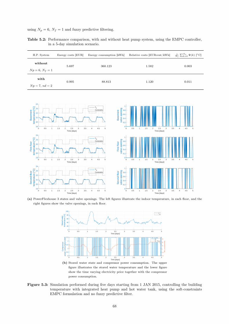
using Np = 6, Nf = 1 and fuzzy predictive filtering.
Table 5.2: Performance comparison, with and without heat pump system, using the EMPC controller,in a 5-day simulation scenario.
H.P. System Energy costs [EUR] Energy consumption [kWh] Relative costs [EURcent/kWh] 1Ns
∑Nsk=0 Ψ(k) [C]
without
Np = 6, Nf = 1
5.697 360.123 1.582 0.003
with
Np = 7, nd = 2
0.995 88.813 1.120 0.011
0 0.5 1 1.5 2 2.5 3 3.5 4 4.5 5
Time [days]
19
20
21
22
23
24
Bas
emen
tte
mpe
ratu
re [°
C] T
b
Constraints
0 0.5 1 1.5 2 2.5 3 3.5 4 4.5 5
Time [days]
19
20
21
22
23
24
Firs
t-flo
orte
mpe
ratu
re [°
C] T
f1
Constraints
0 0.5 1 1.5 2 2.5 3 3.5 4 4.5 5
Time [days]
19
20
21
22
23
24
Sec
ond-
floor
tem
pera
ture
[°C
] Tf2
Constraints
0 0.5 1 1.5 2 2.5 3 3.5 4 4.5 5
Time [days]
0
0.2
0.4
0.6
0.8
1
Bas
emen
tva
lve
open
ing
0 0.5 1 1.5 2 2.5 3 3.5 4 4.5 5
Time [days]
0
0.2
0.4
0.6
0.8
1
Firs
t-flo
orva
lve
open
ing
0 0.5 1 1.5 2 2.5 3 3.5 4 4.5 5
Time [days]
0
0.2
0.4
0.6
0.8
1
Sec
ond-
floor
valv
e op
enin
g
(a) PowerFlexhouse 3 states and valve openings. The left figures illustrate the indoor temperature, in each floor, and theright figures show the valve openings, in each floor.
0 0.5 1 1.5 2 2.5 3 3.5 4 4.5 5
Time [days]
0
20
40
60
80
100
Sto
red
wat
erte
mpe
ratu
re [°
C] T
w
0 0.5 1 1.5 2 2.5 3 3.5 4 4.5 5
Time [days]
0
0.5
1
1.5
2
2.5
Com
pres
sor
pow
er c
onsu
mpt
ion
[kW
]
-40
-20
0
20
40
60Wc
El. Price
(b) Stored water state and compressor power consumption. The upperfigure illustrates the stored water temperature and the lower figureshow the time varying electricity price together with the compressorpower consumption.
Figure 5.3: Simulation performed during five days starting from 1 JAN 2015, controlling the buildingtemperature with integrated heat pump and hot water tank, using the soft-constraintsEMPC formulation and no fuzzy predictive filter.
68

5.6 Discussion
As expected, the results presented in the previous section show that the energy consumption decreasedto about 25%, the energy costs decreased to about 16% and the relative costs, that characterize theenergy shift, decreased to about 67%, comparing to the values of the best performing solution presentedin Chapter 4.
The engineering setup including the heat pump is very efficient, when the COP is kept high. Besides theadvantage of including that system, which already represents a free boost of energy input, the hot watertank system is a very good complement, in a way that it increases the storage capability, increasing thepotential of decreasing the consumption density in peak hours, increasing it in non-peak hours. This isthe reason why the energy cost decreased 5 times and the energy consumption just decreased 3 times.
69


Chapter 6
Conclusions
In this thesis, a new MPC strategy, for managing the heat dynamics of smart buildings, integrated in thefuture energy system, was developed. For this purpose, the designed MPC algorithm, based on nonlinearmodels, considers the nonconvex optimization problem, as well as the economic objective in the costfunction.
The results achieved by the accuracy of the models developed, in Chapter 3, shown the importanceof a previously performed Intelligent Data Analysis, in Chapter 2, applied to dynamic systems-basedproblems, such as control. Thus, the system modeling task can take advantage of a carefully premadedata analysis and preprocessing, such as the one commonly applied in data mining. The CRISP-DMprocess model has shown to be suitable to the type of problem, and justified the importance of lookingat the system as a black-box, in a first stage, identifying the data which has influence on the dynamicsthat is related with this project focus.
As all the model-based control algorithms, the biggest key issue of the MPC development is the modeling.In fact, the model accuracy is what mainly influences the control performance; and to achieve high controlperformances, proper models have to be developed. To do so, in Chapter 3, two different types of grey-box models, based on real measurement data, were developed. Both NLSDE state-space model withintegrated EKF and TS fuzzy model were validated with data, different from the one used for theiridentification, from the four different seasons, showing the performance indexes always above 97% ofVAF and below 0.19C of RMSE.
Chapter 4 is focused on the controller design. A nonlinear EMPC, based on the models developed inChapter 3, was formulated and tested. To create a simulation scenario which is, as similar as possibleto the real-time control case, a model-plant mismatch, using the NLSDE state-space model inside thecontrol algorithm and the TS fuzzy model representing the real system, was considered. The feasibilityunder uncertain scenarios was ensured by introducing soft-constraints into the EMPC formulation anda new type of fuzzy predictive filter, which uses a daily-adaptive MF, based on the CDF of the currentprice signal, was proposed. Indeed, this fuzzy predictive filtering was shown to be capable of reducingthe computation time, by decreasing the control space cardinality, and, at the same time, reducing the
71
load density during peak hours.
To enhance the flexibility that a smart building can provide to the grid, while shifting its load frompeak hours, in Chapter 5, a heat pump coupled with a hot water tank is integrated with the building.Therefore, these systems were modeled, using the NLSDE state-space approach, and afterwards integratedand simulated using the EMPC developed in Chapter 4. It is shown that the introduced system brings upthe advantages of energy consumption decrease and cost reduction, coupled with a higher load shifting,while keeping the comfort level. While developing this solution, it was clear that, even if it was considereda linear dynamics for the building instead, the integration of the hot water tank system introduces anotherstate into the NLSDE formulation, creating a nonlinearity in the global system model. Consequently, thecapability of integration of electricity-heating systems, while considering the nonlinear dynamics due totheir coupling and treating the problem in a centralized fashion for the controller, represents one of thebiggest advantages of this nonlinear EMPC.
Future Work
Pointing out the high importance of the modeling in the developed control solution, and analyzing theportion of time spent in the modeling task, it truly corresponded to about 60%, indicating the big effortthat this process demands. Therefore, globalize a model-based of control solution creates a discussiontopic that should also consider the trade-off between performance and expertise time demand, sinceevery household in the world has different characteristics, and, as a consequence, their models have tobe different from each other. Possibly, seeking the answer for this question will guide the subject to theautomated modeling and machine learning field, in which the Fuzzy Modeling theory is part of. All ofthese facts motivate further research regarding the best way of modeling these systems, e.g. adaptivemodels, grey-box models vs black-box models, and exploring the advantage of machine learning andartificial intelligence based techniques.
The definition of a measurement capable of characterize, in an accurate and consistent way, what thehumans consider as thermal comfort, is a topic of interest among a lot of researchers in the world. Afamous model is the so called Predicted Mean Vote (PMV) index, introduced by [13], which is dependenton a set of factors, such as air temperature, mean radiant temperature, relative humidity, air speed,metabolic rate, and clothing insulation. However, to include this type of adaptive setpoints, the objectivefunction will become highly nonlinear, and the control problem will be transformed in a multi-objectiveand non-convex optimization problem, including the comfort function, as well as the cost function, evenusing linear models for the systems. Although this kind of approach is the most accepted in the com-munity, to represent the thermal comfort using a fuzzy membership grade instead, can improve a lotthe energy savings and the available flexibility, by fuzzifying the optimization membership function andconstraints.
In the present thesis, derivative-free optimization tools to solve the non-convex optimization problem thatshowed up, were proposed, i.e. branch-and-bound. It would be interesting to perform a study comparinghow worse can be the control solution using the commonly used SQP for the same problem. Besidesthat, the developed controller was able to manage the thermal dynamics of one single building, dividingit in three different zones, in a centralized fashion. However, in the user point of view, would be moreinteresting to have different states for each part of the house, allowing them to customize the requirementsof different rooms, depending on the type of room. Therefore, the concept of Distributed MPC seems
72

to be the perfect solution for that problem, including different layers of control levels, even allowingthe possibility of aggregating the control of different smart buildings and take advantage of the coupleddynamics among each other, on the grid side.
The developed EMPC has also shown to be capable of shifting the load from peak hours, increasing theavailable flexibility in the grid. Additionally it would be interesting to see how an aggregation of housescould cooperate to provide flexibility and balancing the system with high penetration of renewables. Inanother angle, a real experiment testing the controller in a real-time control situation should be made,in order to ensure that the controller shows a good performance, although it should be very satisfactory,since the models used are accurate, robustness tests were performed and different king of uncertainties,e.g. model-plant mismatch, forecast errors, and process and measurement noise, were considered.
In conclusion, the nonlinear EMPC presented a good performance for managing the future smart build-ings, reducing costs and offering services to the future grid, what makes it suitable not only for buildings,but also for a wide range of DER units and managing the energy portfolio connected to the smart grid,as e.g. heat pumps, electric vehicles, etc. Together with this type of application, fuzzy predictive filters,specifically personalized for that solution, can be also developed.
Finally, control theory studies, such as stability and robustness, should be carried out. In the particularcase of the developed controller, this is a very important topic, since it operates in a time-varying fashion,making even more critical the verification of those two concepts.
73


Bibliography
[1] Accelera. Heat Pump Water Heaters. [Online] Available: http://www.stiebel-eltron-usa.com/products/accelera-heat-pump-water-heaters (visited on 2016-06-25).
[2] Babuška, R. (1998). Fuzzy Modeling for Control. International Series in Intelligent Technologies.
[3] Babuška, R. (2014). Fuzzy Identification Toolbox for MATLAB (ver. 4.0). [Online] Available:http://www.dcsc.tudelft.nl/˜rbabuska/fmid/fmid-v40.zip (visited on 2016-06-25).
[4] Bergman, T. L., Lavine, A. S., Incropera, F. P., and DeWitt, D. P. (2011). Fundamentals of Heatand Mass Transfer. Seventh edition.
[5] Billings, S. A. and Aguirre, L. A. (1995). Effects of the sampling time on the dynamics and identifi-cation of nonlinear models. International Journal of Bifurcation and Chaos, 5(06):1541–1556.
[6] Butterworth, S. (1930). On the theory of filter amplifiers. Experimental Wireless and the WirelessEngineer, 7:536–541.
[7] Cox, H. (1964). On the estimation of state variables and parameters for noisy dynamic systems. IEEETransactions on Automatic Control, 9(1):5–12.
[8] Curzy, M. (2014). Modeling and System Identification. Technical report, Technical University ofDenmark.
[9] Delff, P., Madsen, H., Bacher, P., and Nielsen, H. A. (2011). Improved experimental setup forobservation of non-linear heat dynamics. Arctic, pages 1–8.
[10] DTU Compute. CTSM-R – Continuous Time Stochastic Modelling for R. [Online] Available:http://ctsm.info/pdfs/ctsmr-reference.pdf (visited on 2016-04-30).
[11] DTU Departement of Wind Energy. Weather Forecast Data: Risø. [Online] Available:http://www.vindenergi.dtu.dk/english (visited on 2016-05-26).
[12] Energinet.dk. Energinet.dk. [Online] Available: http://energinet.dk/EN/Sider/default.aspx (visitedon 2016-06-30).
[13] Fanger, P. O. (1970). Thermal Comfort: Analysis and applications in environmental engineering.Danish Technical Press.
[14] Ferreira, P. M., Ruano, A. E., Silva, S., and Conceição, E. Z. E. (2012). Neural networks basedpredictive control for thermal comfort and energy savings in public buildings. Energy and Buildings,55:238–251.
75
[15] Halvgaard, R., Poulsen, N. K., Madsen, H., and Jorgensen, J. B. (2012). Economic Model PredictiveControl for building climate control in a Smart Grid. In 2012 IEEE PES Innovative Smart GridTechnologies (ISGT), pages 1–6.
[16] Hand, D. J. (1998). Intelligent Data Analysis: Issues and Opportunities. Intelligent Data Analysis,2(2).
[17] Haykin, S. O. (2009). Neural Networks and Learning Machines. Third edition.
[18] Hong, J., Kelly, N. J., Richardson, I., and Thomson, M. (2012). Assessing heat pumps as flexibleload. In Proceedings of the Institution of Mechanical Engineers, Part A: Journal of Power and Energy,volume 227, pages 30–42.
[19] Hovgaard, T., Edlund, K., and Jørgensen, J. (2010). The potential of Economic MPC for powermanagement. In 49th IEEE Conference on Decision and Control (CDC), pages 7533–7538.
[20] Hovgard, T. G., Larsen, L. F. S., Jørgensen, J. B., and Boyd, S. (2012). Fast nonconvex model pre-dictive control for commercial refrigeration. IFAC Proceedings Volumes (IFAC-PapersOnline), 4(PART1):514–521.
[21] Huang, H., Chen, L., and Hu, E. (2015). A hybrid model predictive control scheme for energy andcost savings in commercial buildings: simulation and experiment.
[22] Hydrogenious Technologies. The Breakthrough of Global Energy Storage. [Online] Available:http://www.hydrogenious.net (visited on 2016-07-03).
[23] International Energy Agency (2013). Transition to Sustainable Buildings – Strategies and Opportu-nities to 2050. 2013 edition.
[24] International Energy Agency (2015). Key World Energy Statistics 2015. 2015 edition.
[25] International Energy Agency (2016). Re-powering Markets: Market design and regulation during thetransition to low-carbon power systems. 2016 edition.
[26] Jiménez, M. J., Madsen, H., Bloem, J. J., and Dammann, B. (2008). Estimation of non-linearcontinuous time models for the heat exchange dynamics of building integrated photovoltaic modules.Energy and Buildings, 40(2):157–167.
[27] Jolliffe, I. T. and Stephenson, D. B. (2003). Forecast Verification: A Practitioner’s Guide in Atmo-spheric Science. 2nd edition.
[28] Kalman, R. (1960). A new approach to linear filtering and prediction problems. Journal of basicEngineering, 82(1):35–45.
[29] Kurzweil, R. (2005). The Singularity Is Near: When Humans Transcend Biology.
[30] Lamoudi, M. Y., Alamir, M., and Béguery, P. (2011). Distributed constrained Model PredictiveControl based on bundle method for building energy management. In 50th IEEE Conference onDecision and Control, pages 8118–8124.
[31] Liu, X., Jenkins, N., Wu, J., and Bagdanavicius, A. (2014). Combined analysis of electricity andheat networks. Energy Procedia, 61:155–159.
[32] Liu, X. and Mancarella, P. (2016). Modelling, assessment and Sankey diagrams of integratedelectricity-heat-gas networks in multi-vector district energy systems. Applied Energy, 167:336–352.
76

[33] Maciejowski, J. M. (2002). Predictive control: with constraints, Pearson Hall. Pearson Education.
[34] Marshall, A. (1890). Principles of Economics, Macmillan and Company, volume 1. 8th edition.
[35] Mendonça, L. F., Sousa, J. M., and Sá Da Costa, J. M. G. (2004). Optimization problems inmultivariable fuzzy predictive control. International Journal of Approximate Reasoning, 36(3):199–221.
[36] Millar, R. B. (2011). Maximum Likelihood Estimation And Inference. John Wiley & Sons, firstedition.
[37] Moore, G. E. (1965). Cramming more components onto integrated circuits. Electronics, pages114–117.
[38] Moran, M. J., Shappiro, H. N., Boettner, D. D., and Bailey, M. B. (2010). Fundamentals of Engi-neering Thermodynamics, volume 1. Seventh edition.
[39] Nord Pool. The Nord Pool spot market. [Online] Available:http://www.nordpoolspot.com/historical-market-data (visited on 2016-06-30).
[40] Nyquist, H. (1928). Certain topics in telegraph transmission theory. Transactions of the AIEE,47(2):617–644.
[41] Øksendal, B. (1993). Stochastic Differential Equations, Linear Filtering, and Chaos Expansion,Annals Of The New York Academy Of Sciences, volume 706.
[42] Oldewurtel, F., Parisio, A., Jones, C., Morari, M., Gyalistras, D., Gwerder, M., Stauch, V., Lehmann,B., and Wirth, K. (2010). Energy efficient building climate control using Stochastic Model PredictiveControl and weather predictions. In American Control Conference, pages 5100–5105.
[43] PowerLabDK. SYSLAB. [Online] Available: http://www.powerlab.dk/facilities/syslab (visited on2016-07-24).
[44] Purmo. Effekt beregningsprogram. [Online] Available: http://www.purmo.com/dk/downloads/effekt-beregningsprogram.htm (visited on 2016-06-25).
[45] Richalet, J. (1993). Industrial applications of model based predictive control. Automatica,29(5):1251–1274.
[46] Ruano, A. E., Pesteh, S., Silva, S., Duarte, H., Mestre, G., Ferreira, P. M., Khosravani, H. R., andHorta, R. (2016). The IMBPC HVAC system: A complete MBPC solution for existing HVAC systems.Energy and Buildings, 120:145–158.
[47] Ruelens, F., Claessens, B. J., Vandael, S., De Schutter, B., Babuska, R., and Belmans, R. (2016).Residential demand response of thermostatically controlled loads using batch reinforcement learning.IEEE Transactions on Smart Grid, pages 1–11.
[48] Santos, R. M., Zong, Y., Sousa, J. M. C., and Mendonça, L. (2016). Nonlinear Economic ModelPredictive Control for Smart Buildings: A Centralized Approach for the Integration of Electricity andHeating. To Be Submitted, by October, to Applied Energy.
[49] Santos, R. M., Zong, Y., Sousa, J. M. C., Mendonça, L., and Thavlov, A. (2016). Nonlinear EconomicModel Predictive Control Strategy for Active Smart Buildings. In 2016 IEEE PES Innovative SmartGrid Technologies, Europe, 9-12 Ljubljana.
77

[50] Santos, R. M., Zong, Y., Sousa, J. M. C., Mendonça, L., You, S., and Mihet-Popa, L. (2016). FuzzyPredictive Filtering in Nonlinear Economic Model Predictive Control for Demand Response. In 2016IEEE Electrical Power and Energy Conference, 12-14 Ottawa.
[51] Schibuola, L., Scarpa, M., and Tambani, C. (2015). Demand response management by means of heatpumps controlled via real time pricing. Energy and Buildings, 90:15–28.
[52] Shearer, C. (2000). The CRISP-DM model: The New Blueprint for Data Mining. Journal of DataWarehousing14, 5(4):13–22.
[53] Sousa, J. M., Babuška, R., and Verbruggen, H. B. (1997). Fuzzy predictive control applied to anair-conditioning system. Control Engineering Practice, 5(10):1395–1406.
[54] Sousa, J. M. and Setnes, M. (1999). Fuzzy predictive filters in model predictive control. IEEETransactions on Industrial Electronics, 46(6):1225–1232.
[55] Sousa, J. M. C. and Kaymak, U. (2002). Fuzzy decision making in modeling and control, WorldScientific Series in Robotics and Intelligent Systems, volume 27.
[56] Svendsen, M. (2013). Extension of Home Automation Platform for Demand Side Management of aSmart House. PhD thesis, Technical University of Denmark.
[57] Takagi, T. and Sugeno, M. (1985). Fuzzy Identification of Systems and Its Aplications to Modelingand Control. IEEE Transactions on Sysyems, Man and Cybernetics, 15(1):116–132.
[58] Thavlov, A. and Madsen, H. (2015). A Non-linear Stochastic Model for an Office Building with Air.Journal, International Planning, Sustainable Energy Vol, Management, 07:59–70.
[59] The Engineering ToolBox. Overall Heat Transfer Coefficients for some Fluids and Heat ExchangerSurfaces. [Online] Available: http://www.engineeringtoolbox.com/overall-heat-transfer-coefficients-d_284.html (visited on 2016-07-01).
[60] Tran, T., Ling, K.-V., and Maciejowski, J. M. (2014). Economic Model Predictive Control - AReview. In The 31st International Symposium on Automation and Robotics in Construction andMining (ISARC 2014), pages 35–42.
[61] van Hoof, J. and Hensen, J. L. M. (2007). Quantifying the relevance of adaptive thermal comfortmodels in moderate thermal climate zones. Building and Environment, 42(1):156–170.
[62] Zadeh, L. A. (1965). Fuzzy Sets. Information and Control, 8(3):338–353.
[63] Zong, Y., Böning, G. M., Santos, R. M., You, S., Hu, J., and Han, X. (2016). Challenges of Im-plementing Economic Model Predictive Control Strategy for Buildings Interacting with Smart EnergySystems. Submitted to Applied Thermal Engineering.
[64] Zong, Y., Kullmann, D., Thavlov, A., Gehrke, O., and Bindner, H. (2012). Application of ModelPredictive Control for Active Load Management in a Distributed Power System With High WindPenetration. IEEE Transactions on Smart Grid, 3(2):1055–1062.
78

Appendices
79


Appendix A
Data Summary
81
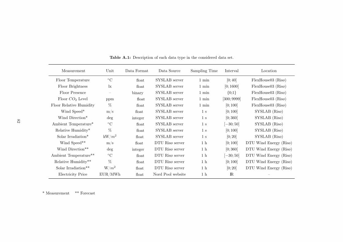
Table A.1: Description of each data type in the considered data set.
Measurement Unit Data Format Data Source Sampling Time Interval Location
Floor Temperature C float SYSLAB server 1 min [0; 40] FlexHouse03 (Risø)Floor Brightness lx float SYSLAB server 1 min [0; 1600] FlexHouse03 (Risø)Floor Presence – binary SYSLAB server 1 min 0;1 FlexHouse03 (Risø)Floor CO2 Level ppm float SYSLAB server 1 min [300; 9999] FlexHouse03 (Risø)
Floor Relative Humidity % float SYSLAB server 1 min [0; 100] FlexHouse03 (Risø)Wind Speed* m/s float SYSLAB server 1 s [0; 100] SYSLAB (Risø)
Wind Direction* deg integer SYSLAB server 1 s [0; 360[ SYSLAB (Risø)Ambient Temperature* C float SYSLAB server 1 s [−30; 50] SYSLAB (Risø)Relative Humidity* % float SYSLAB server 1 s [0; 100] SYSLAB (Risø)Solar Irradiation* kW/m2 float SYSLAB server 1 s [0; 20] SYSLAB (Risø)Wind Speed** m/s float DTU Risø server 1 h [0; 100] DTU Wind Energy (Risø)
Wind Direction** deg integer DTU Risø server 1 h [0; 360[ DTU Wind Energy (Risø)Ambient Temperature** C float DTU Risø server 1 h [−30; 50] DTU Wind Energy (Risø)Relative Humidity** % float DTU Risø server 1 h [0; 100] DTU Wind Energy (Risø)Solar Irradiation** W/m2 float DTU Risø server 1 h [0; 20] DTU Wind Energy (Risø)Electricity Price EUR/MWh float Nord Pool website 1 h IR –
* Measurement ** Forecast
82

Appendix B
Sensor and Actuator Location
83


Appendix C
PowerFlexhouse 3: Heating Power
Distribution
Assuming the supply water always keeps the constant value of 70C and the mean value for the innerair temperature is about 20C the max power distribution in each water-based radiator is presented inTable C.1.
Table C.1: Maximum heat power (kW) distribution among each floor, together with total equivalentpower.
Radiator Basement First-floor Second-floor
Type 1 0.327 - -Type 2 - 5.128 0.916Type 3 1.099 - -Type 4 1.282 - 1.282Type 5 - 1.010
Total 2.708 6.138 2.198
87


Appendix D
Extended Kalman Filter – Matrices
To implement the hybrid EKF solution presented in Section 3.3.2 to the NLSDE state-space modelintroduced in Section 3.3, the Jacobian A(t) and the Ck are two quantities that have to be computed inan offline fashion. The results are given by
A(t) =∂f(x,ut, t,θ)
∂x
∣∣∣∣x=xt|k
=
=
A11 A12 A13 A14 A15 A16
A21 A22 A23 A24 A25 A26
A31 A32 A33 A34 A35 A36
A41 A42 A43 A44 A45 A46
A51 A52 A53 A54 A55 A56
A61 A62 A63 A64 A65 A66
(D.1)
89
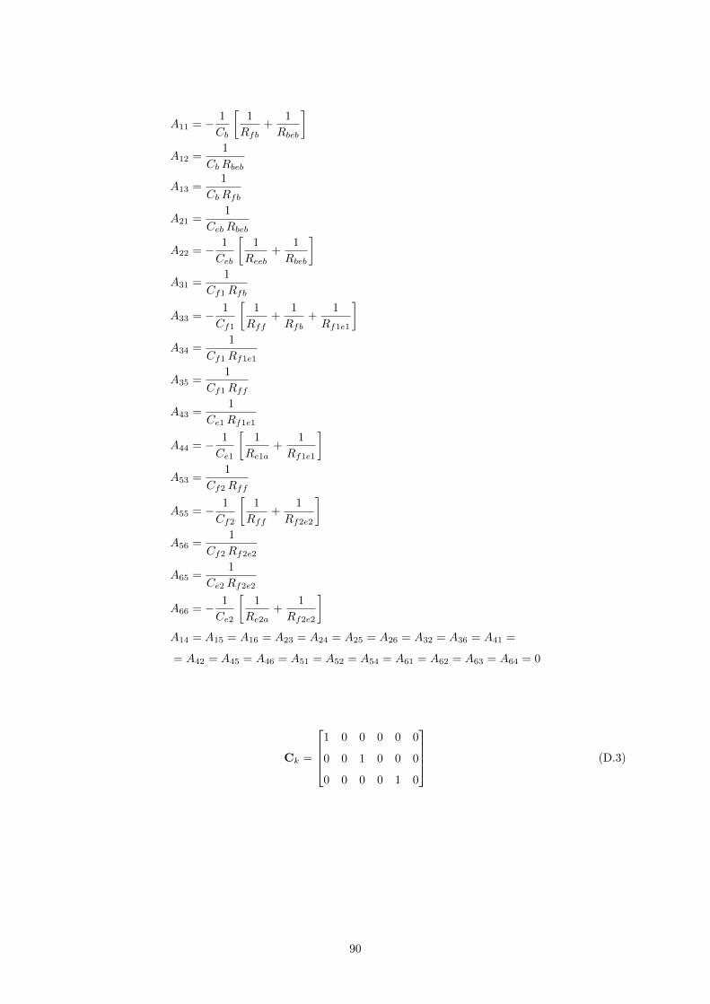
A11 = − 1
Cb
[1
Rfb+
1
Rbeb
]A12 =
1
CbRbeb
A13 =1
CbRfb
A21 =1
CebRbeb
A22 = − 1
Ceb
[1
Reeb+
1
Rbeb
]A31 =
1
Cf1Rfb
A33 = − 1
Cf1
[1
Rff+
1
Rfb+
1
Rf1e1
]A34 =
1
Cf1Rf1e1
A35 =1
Cf1Rff
A43 =1
Ce1Rf1e1
A44 = − 1
Ce1
[1
Re1a+
1
Rf1e1
]A53 =
1
Cf2Rff
A55 = − 1
Cf2
[1
Rff+
1
Rf2e2
]A56 =
1
Cf2Rf2e2
A65 =1
Ce2Rf2e2
A66 = − 1
Ce2
[1
Re2a+
1
Rf2e2
]A14 = A15 = A16 = A23 = A24 = A25 = A26 = A32 = A36 = A41 =
= A42 = A45 = A46 = A51 = A52 = A54 = A61 = A62 = A63 = A64 = 0
Ck =
1 0 0 0 0 0
0 0 1 0 0 0
0 0 0 0 1 0
(D.3)
90

Appendix E
Model Validation – Plots
91
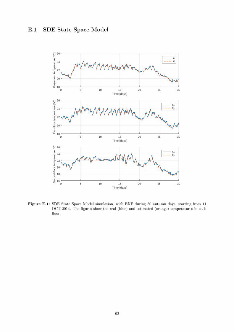
E.1 SDE State Space Model
0 5 10 15 20 25 30
Time [days]
18
20
22
24
26B
asem
ent t
empe
ratu
re [º
C]
Tb
Tb
0 5 10 15 20 25 30
Time [days]
18
20
22
24
26
Firs
t-flo
or te
mpe
ratu
re [º
C]
Tf1
Tf1
0 5 10 15 20 25 30
Time [days]
16
18
20
22
24
26
Sec
ond-
floor
tem
pera
ture
[ºC
]
Tf2
Tf2
Figure E.1: SDE State Space Model simulation, with EKF during 30 autumn days, starting from 11OCT 2014. The figures show the real (blue) and estimated (orange) temperatures in eachfloor.
92
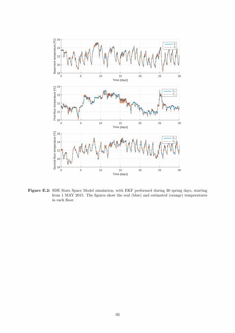
0 5 10 15 20 25 30
Time [days]
18
20
22
24
26
Bas
emen
t tem
pera
ture
[ºC
]
Tb
Tb
0 5 10 15 20 25 30
Time [days]
20
21
22
23
24
Firs
t-flo
or te
mpe
ratu
re [º
C]
Tf1
Tf1
0 5 10 15 20 25 30
Time [days]
18
20
22
24
26
Sec
ond-
floor
tem
pera
ture
[ºC
]
Tf2
Tf2
Figure E.2: SDE State Space Model simulation, with EKF performed during 30 spring days, startingfrom 1 MAY 2015. The figures show the real (blue) and estimated (orange) temperaturesin each floor.
93
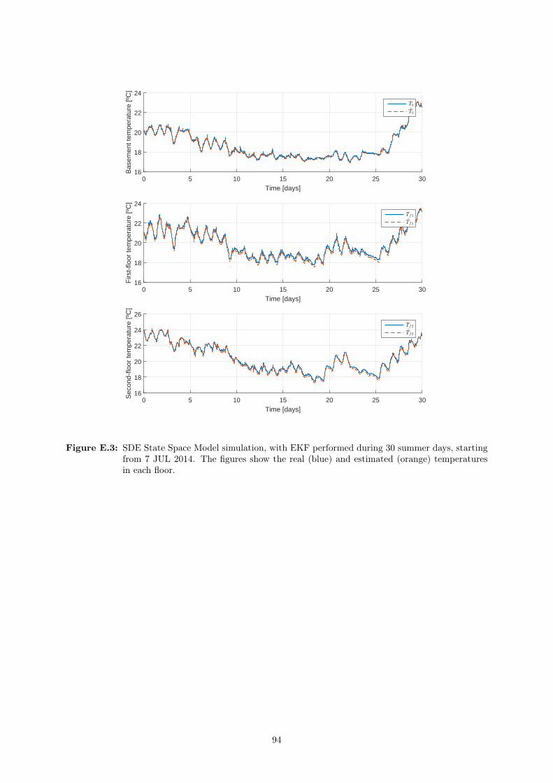
0 5 10 15 20 25 30
Time [days]
16
18
20
22
24
Bas
emen
t tem
pera
ture
[ºC
]
Tb
Tb
0 5 10 15 20 25 30
Time [days]
16
18
20
22
24
Firs
t-flo
or te
mpe
ratu
re [º
C]
Tf1
Tf1
0 5 10 15 20 25 30
Time [days]
16
18
20
22
24
26
Sec
ond-
floor
tem
pera
ture
[ºC
]
Tf2
Tf2
Figure E.3: SDE State Space Model simulation, with EKF performed during 30 summer days, startingfrom 7 JUL 2014. The figures show the real (blue) and estimated (orange) temperaturesin each floor.
94
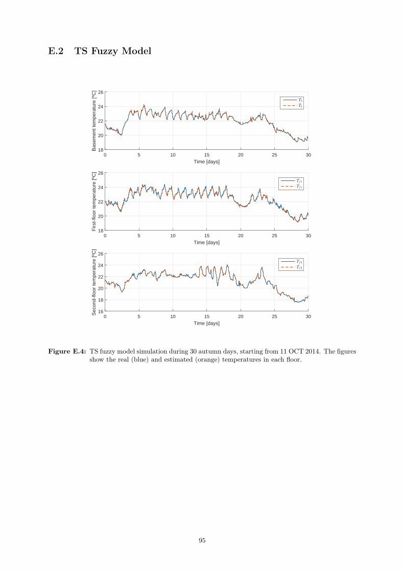
E.2 TS Fuzzy Model
0 5 10 15 20 25 30
Time [days]
18
20
22
24
26B
asem
ent t
empe
ratu
re [º
C]
Tb
Tb
0 5 10 15 20 25 30
Time [days]
18
20
22
24
26
Firs
t-flo
or te
mpe
ratu
re [º
C]
Tf1
Tf1
0 5 10 15 20 25 30
Time [days]
16
18
20
22
24
26
Sec
ond-
floor
tem
pera
ture
[ºC
]
Tf2
Tf2
Figure E.4: TS fuzzy model simulation during 30 autumn days, starting from 11 OCT 2014. The figuresshow the real (blue) and estimated (orange) temperatures in each floor.
95
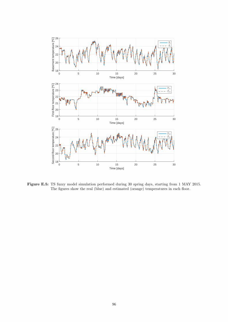
0 5 10 15 20 25 30
Time [days]
18
20
22
24
26
Bas
emen
t tem
pera
ture
[ºC
]
Tb
Tb
0 5 10 15 20 25 30
Time [days]
19
20
21
22
23
24
Firs
t-flo
or te
mpe
ratu
re [º
C]
Tf1
Tf1
0 5 10 15 20 25 30
Time [days]
18
20
22
24
26
Sec
ond-
floor
tem
pera
ture
[ºC
]
Tf2
Tf2
Figure E.5: TS fuzzy model simulation performed during 30 spring days, starting from 1 MAY 2015.The figures show the real (blue) and estimated (orange) temperatures in each floor.
96
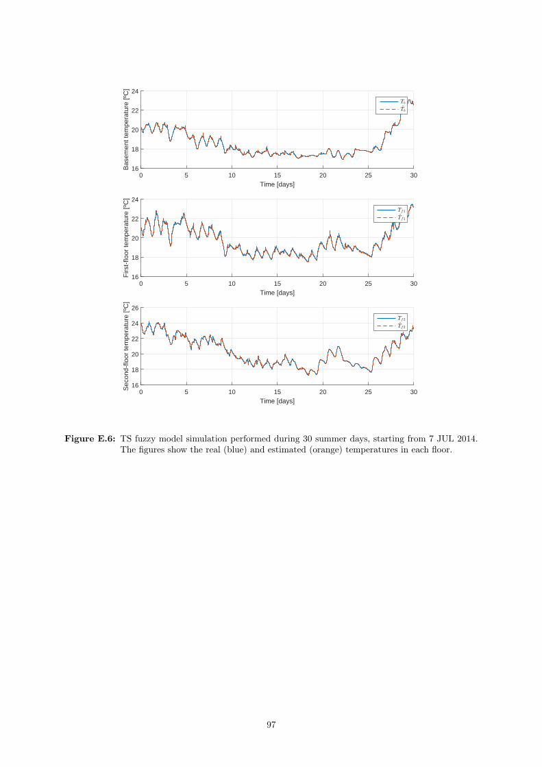
0 5 10 15 20 25 30
Time [days]
16
18
20
22
24
Bas
emen
t tem
pera
ture
[ºC
]
Tb
Tb
0 5 10 15 20 25 30
Time [days]
16
18
20
22
24
Firs
t-flo
or te
mpe
ratu
re [º
C]
Tf1
Tf1
0 5 10 15 20 25 30
Time [days]
16
18
20
22
24
26
Sec
ond-
floor
tem
pera
ture
[ºC
]
Tf2
Tf2
Figure E.6: TS fuzzy model simulation performed during 30 summer days, starting from 7 JUL 2014.The figures show the real (blue) and estimated (orange) temperatures in each floor.
97


Appendix F
Branch-and-bound algorithm for
EMPC
99

Algorithm 1 Branch-and-bound algorithm for EMPC
Setup Controller: Choose the prediction horizon Np; the values for the input constraints umin, umax,∆umin and ∆umax; the values for the output constraints ymin and ymax; and the number of discretecontrol actions nd.
Real Time: t = k Ts
1: Estimate upper bound At each level k + j, with j = 0, . . . , Np − 1, choose the smallest J (j)i (µi).
The initial upper bound is then JU =∑Np−1j min
(J
(j)i (µi)
).
2: Set: j = 0
3: if Current state j is fully explored4: if j = 0
5: return u∗(0)k = µ
∗(0)i Use the receding horizon principle, applying the optimal control action.
6: end if7: j ←− j + 1
8: Go to step 39: else
10: for i = 1 to nd
11: if j = 0
12: J(j)c,i = 0
13: else14: J
(j)c,i = J
(j−1)c,i + J
(j)i (µ)
15: end if16: end for17: for i = 1 to nd Sorted by increasing cost and number of explorations.18: if J
(j)c,i < JU and j < Np− 1
19: Branch: j µi−→ j + 1
20: Go to step 321: end if22: if J
(j)c,i < JU and j = Np− 1
23: JU = J(j)c,i
24: end if25: end for26: end if
100

Appendix G
Heat Pump Specifications
101
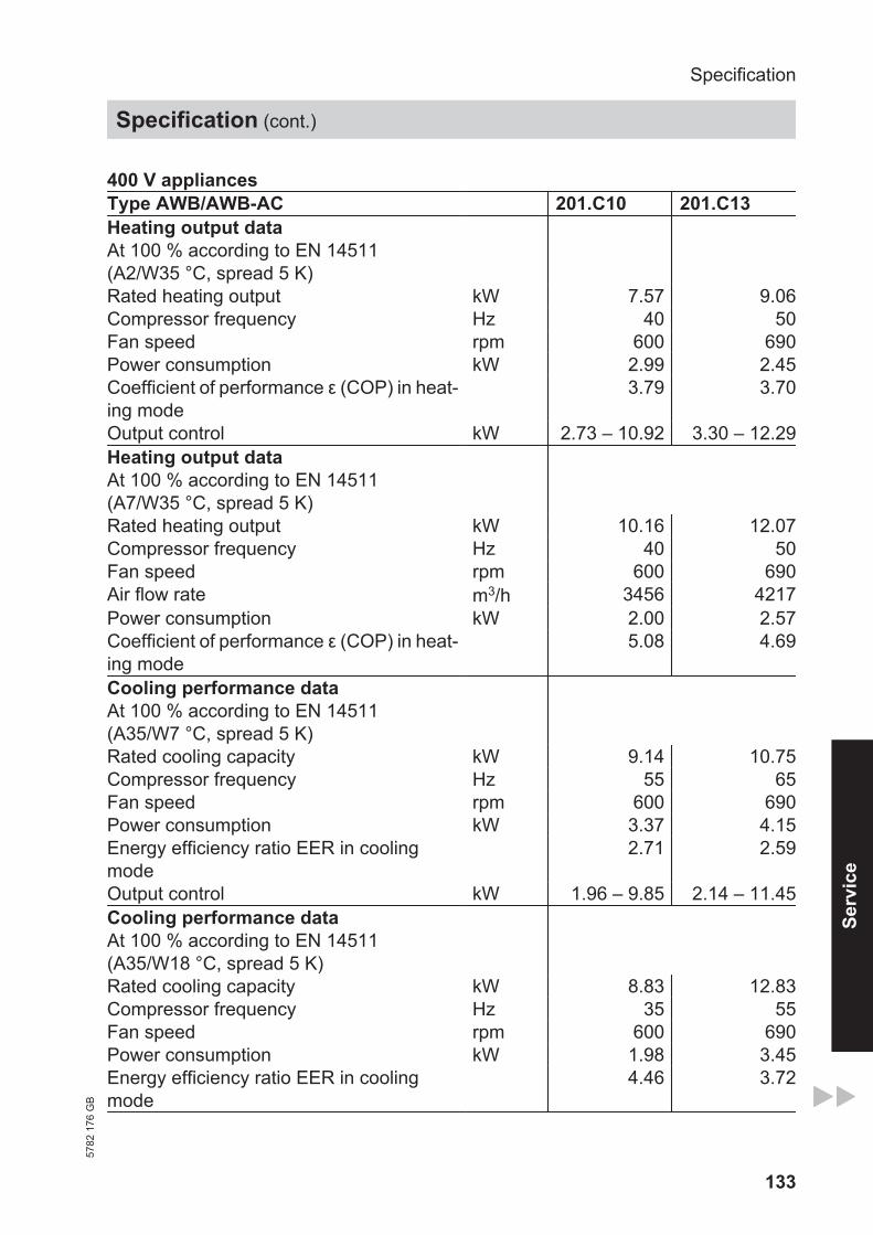
133
400 V appliancesType AWB/AWB-AC 201.C10 201.C13Heating output dataAt 100 % according to EN 14511(A2/W35 °C, spread 5 K)
Rated heating output kW 7.57 9.06Compressor frequency Hz 40 50Fan speed rpm 600 690Power consumption kW 2.99 2.45Coefficient of performance ε (COP) in heat-ing mode
3.79 3.70
Output control kW 2.73 – 10.92 3.30 – 12.29Heating output dataAt 100 % according to EN 14511(A7/W35 °C, spread 5 K)
Rated heating output kW 10.16 12.07Compressor frequency Hz 40 50Fan speed rpm 600 690Air flow rate m3/h 3456 4217Power consumption kW 2.00 2.57Coefficient of performance ε (COP) in heat-ing mode
5.08 4.69
Cooling performance dataAt 100 % according to EN 14511(A35/W7 °C, spread 5 K)
Rated cooling capacity kW 9.14 10.75Compressor frequency Hz 55 65Fan speed rpm 600 690Power consumption kW 3.37 4.15Energy efficiency ratio EER in coolingmode
2.71 2.59
Output control kW 1.96 – 9.85 2.14 – 11.45Cooling performance dataAt 100 % according to EN 14511(A35/W18 °C, spread 5 K)
Rated cooling capacity kW 8.83 12.83Compressor frequency Hz 35 55Fan speed rpm 600 690Power consumption kW 1.98 3.45Energy efficiency ratio EER in coolingmode
4.46 3.72
Specification
Specification (cont.)
5782
176
GB
Serv
ice

Appendix H
Water Tank Specifications
103

4
1.8 Maintenance and cleaningThe device is generally maintenance free, with the exception of cleaning the strainer in the condensate drain.
Sand and dust can result in sludge building up inside the strainer. Therefore, clean the strainer at least twice per annum or in accordance with demand.
A damp cloth is sufficient for cleaning all plastic parts. Never use scouring or solvent-based cleaning agents.
!Please note: Maintenance work, e.g. checking the electrical safety,
must only be carried out by a qualified contractor.
z Check the condensate drain at least monthly at the bottom strainer outlet and at the top condensate pan drain (visual check, see Fig. 3 and Fig. 4, pos. 15). Remove contaminants and blockages immediately.
z For the WWK300 AH and WWK300 AHP, it is recommended that the electric booster heater be descaled from time to time. This will result in prolonged life fo the electric booster.
z Your local contractor, who is familiar with the local water quality, should identify for you the timing of the next service.
z Ask your local contractor to regularly check the safety assembly and the electric booster heater.
z The device is subject to mains water pressure. The expansion water drips from the safety valve during heat-up. Inform your local contractor of water drips from the system after the heat-up process has ended.
z To protect the steel cylinder against corrosion, the interior is coated with a special enamel and is furthermore equipped with a protective anode. Ask your local contractor to check the protective anode regularly.
1.9 Troubleshooting by the user
No hot water
Should you fail to obtain hot water at any time, you can take the following steps to remedy that situation.
No electrical power Check the fuse/circuit breaker in your fuse box. If it has blown/tripped, replace/reset the fuse/MCB. If it should blow/trigger repeatedly, notify your local contractor.
Still no hot water, even though power is available Check, whether the air inlet/outlet is blocked.
The thermoswitch trips out or the high limit safety pressure limiter switches the compressor OFF if the compressor is overloaded due to excessive ambient temperature or excessive air temperature (>42 °C), or because of a fault in the refrigerant circuit. Ask your local contractor to remove the fault.
After a short cooldown phase, the thermoswitch will restart the compressor automatically.
!The high limit safety pressure limiter must only be reset by your
contractor after he has removed the cause of the relevant fault.
Other issues
Safety valve of the cold water supply line drips This may occur during the heat-up phase and is completely normal.
The condensate drain drips This always happens when the surface temperature of the evaporator is lower than the ambient dew point temperature.
For all other faults, consult your contractor.

5
22-6
0 ad
just
able
2.1 Regulations and standards
z The installation (water and electrical work) and commissioning, as well as the maintenance of this equipment, must only be carried out by an authorised qualified contractor in accordance with these instructions.
z Perfect function and safe operation can only be assured when using original accessories and spare parts intended for this equipment.
z DIN VDE 0100 / DIN VDE 0701
z Regulations of your local electricity supply utility.
z DIN 1988 / DIN 4109
z Regulations of your local water supply utility.
Fig. 1
2. Installation instructions for contractors
The following standards were taken into account:
AS 4234, AS 3498, AS 4020, AS 1056.1
AS/NZS 2712, AS/NZS 3350.2.40/30/30.2
IEC 60335-1-2-40, IEC 61000-3-2; 1995
IEC 61000-3-3, IEC 55014-1 IEC 55014-2
EMC Directive 89/336/EEC
EN 255 T3
48°
30°10°
1 Cold water supply R 1“ (3/4“ female with adapter)
2 Hot water connection R 1“ (3/4“ female with adapter)
3 Condensate drain ¾“ hose connection
4 Connection for P&T relief valve R ¾“ (on-site)
5 Electrical cable (without plug)
6 Drain valve (on-site)
7 Expansion control valve (if required*, on-site)
8 Straight-through shut-off valve (on-site)
9 Pressure gauge test connector (on-site)
10 Non-return valve (on-site)
11 Test valve connection (on-site)
12 Pressure reducing valve (on-site)
12 10116 898
7
3
1
2
Dimensions in mm
Connection dimensions and variations
5
DHW
Cold water
4
1695
1265
3
1840
5
26_0
3_01
_074
0
Also observe the following:
z The equipment type plate
z The specification
z Water installation
— Observe the AS/NZS 3500. [local regulations].
— Material of the cold water line: Steel, copper or plastic pipe systems.
— Material of the hot water line: Copper or plastic pipe systems.
58
* Not all local regulations require the use of an ex-pansion control valve (ECV).

[This page intentionally left blank]
106

[This page intentionally left blank]
107