Embed Size (px)
Citation preview

Noise generation in vehicle brakes
Cambridge University
Engineering Department
A dissertation submitted to the University of Cambridge for the degree of Doctor of
Philosophy.
by
Philippe Duffour
Jesus College, Cambridge
December 2002

ii

Declaration
This dissertation describes part of the research performed at Cambridge University Engi-
neering Department between May 1999 and December 2002. It is the result of my own
work and includes nothing which is the outcome of work done in collaboration. It contains
approximately 60 000 words and 100 figures.
iii

iv DECLARATION

Summary
Brake noise has been a problem ever since the appearance of automotive vehicles. This
dissertation is concerned with better understanding the underlying mechanisms behind the
phenomenon. To this end, the stability of a class of simplified systems is investigated. This
class of system consists of any two linear subsystems in sliding contact at a single point.
The stability analysis surveys all possible routes to instability which can be formulated
within linear theory. For each route to instability, a criterion is derived in terms of matrices
of transfer functions defined at the contact point. The stability of the coupled system is
investigated numerically by simulating the behaviour of generic systems.
The conclusions are that with a constant coefficient of friction, the occurrence of instability
can be linked to the presence of three modes of the uncoupled subsystems with consecutive
frequencies and generating displacements at the contact point with the appropriate pattern
of signs.
A compliant contact was identified as another possible route to instability. This was mod-
elled by including linear contact springs at the interfaces. Simulations showed that contact
compliance could have a significant effect whenever the stiffness of the contact is of the same
order of magnitude or below the bulk structural stiffness of the system.
Non-proportional damping was also investigated as a possible cause of instability and proved
to have unexpected consequences in that it can cause the governing quantities to grow
exponentially.
A final route to instability was investigated in allowing the coefficient of friction to vary
linearly with sliding speed. Simulated examples were studied and a dimensionless quantity
was derived, indicating when this effect is expected to be significant.
Finally, stability predictions obtained using a constant coefficient of friction were compared
with experimental results obtained from a specially designed rig. Instability could be pre-
dicted in 75 % of the cases.
v

vi SUMMARY

Acknowledgement
I am very grateful to my supervisor, Professor Jim Woodhouse for his ever enthusiastic
guidance and his availability throughout these years of research at Cambridge.
I would like to express my gratitude to Bosch Braking System at Drancy and Bosch Corporate
Research at Stuttgart for providing the financial support of my research. I would to thank
Roland Pitteroff without whom this collaboration would have never happened.
I am also grateful to Professor Ken Johnson, Professor Robin Langley and Dr. David Cole
for helpful discussions.
For help in producing my experimental apparatus, I would like to thank Mr David Miller
and all the staff of the Mechanics Laboratory.
I am thankful to my colleagues in the Mechanics Group as well as the administrative staff of
the Engineering Department for providing a congenial working atmosphere and for making
the conditions for a PhD ideal.
vii

viii ACKNOWLEDGEMENT

Contents
Declaration iii
Summary v
Acknowledgement vii
1 A Review Of Literature 1
1.1 Introduction . . . . . . . . . . . . . . . . . . . . . . . . . . . . . . . . . . . . 1
1.2 Tribological Background . . . . . . . . . . . . . . . . . . . . . . . . . . . . . 1
1.2.1 Friction Phenomena . . . . . . . . . . . . . . . . . . . . . . . . . . . 1
1.2.2 Background work on friction-induced vibration . . . . . . . . . . . . . 5
1.2.3 Normal Degree of Freedom . . . . . . . . . . . . . . . . . . . . . . . . 10
1.2.4 Rock Mechanics Contribution . . . . . . . . . . . . . . . . . . . . . . 11
1.2.5 Bowed-string vibration . . . . . . . . . . . . . . . . . . . . . . . . . . 12
1.2.6 Concluding Remark . . . . . . . . . . . . . . . . . . . . . . . . . . . . 12
1.3 Structural models for brake noise . . . . . . . . . . . . . . . . . . . . . . . . 13
1.3.1 Sprag-Slip . . . . . . . . . . . . . . . . . . . . . . . . . . . . . . . . . 13
1.3.2 Simplified Multiple Degree of Freedom Systems . . . . . . . . . . . . 14
1.3.3 Systems with extended contact . . . . . . . . . . . . . . . . . . . . . 17
1.4 Loaded disc . . . . . . . . . . . . . . . . . . . . . . . . . . . . . . . . . . . . 18
1.4.1 Vibration of a stationary disc . . . . . . . . . . . . . . . . . . . . . . 18
1.4.2 Vibration of a rotating disc . . . . . . . . . . . . . . . . . . . . . . . 20
1.4.3 Pin-loaded discs . . . . . . . . . . . . . . . . . . . . . . . . . . . . . . 22
1.4.4 Loaded disc with friction force. . . . . . . . . . . . . . . . . . . . . . 24
1.5 Experimental studies . . . . . . . . . . . . . . . . . . . . . . . . . . . . . . . 26
1.5.1 Tribological properties of the disc-pad interface . . . . . . . . . . . . 26
1.5.2 Vibration-based experiments . . . . . . . . . . . . . . . . . . . . . . . 27
1.6 Conclusion and outline of the dissertation . . . . . . . . . . . . . . . . . . . 35
2 Study of a pin-on-disc lumped-parameter model 39
2.1 Introduction . . . . . . . . . . . . . . . . . . . . . . . . . . . . . . . . . . . . 39
2.2 Two degree-of-freedom model . . . . . . . . . . . . . . . . . . . . . . . . . . 39
2.2.1 Case without damping . . . . . . . . . . . . . . . . . . . . . . . . . . 41
ix

x CONTENTS
2.2.2 Case with damping . . . . . . . . . . . . . . . . . . . . . . . . . . . . 47
2.2.3 Conclusion . . . . . . . . . . . . . . . . . . . . . . . . . . . . . . . . . 53
2.3 Three degree-of-freedom model . . . . . . . . . . . . . . . . . . . . . . . . . 53
2.3.1 Conclusion for the three-degree-of-freedom model . . . . . . . . . . . 60
2.4 Conclusion . . . . . . . . . . . . . . . . . . . . . . . . . . . . . . . . . . . . . 61
3 Theory of linear instability in systems with a sliding point contact 63
3.1 Introduction . . . . . . . . . . . . . . . . . . . . . . . . . . . . . . . . . . . . 63
3.2 Governing equations . . . . . . . . . . . . . . . . . . . . . . . . . . . . . . . 64
3.3 Some general observations . . . . . . . . . . . . . . . . . . . . . . . . . . . . 66
3.3.1 Cross-term of the disc . . . . . . . . . . . . . . . . . . . . . . . . . . 66
3.3.2 Expression of D(ω) in terms of modal parameters . . . . . . . . . . . 67
3.3.3 The algebraic point of view . . . . . . . . . . . . . . . . . . . . . . . 68
3.3.4 The complex analysis point of view . . . . . . . . . . . . . . . . . . . 69
3.3.5 Application to the pin-on-disc system . . . . . . . . . . . . . . . . . . 71
3.3.6 Summary of the general properties . . . . . . . . . . . . . . . . . . . 72
3.4 Approximate analysis of generic systems . . . . . . . . . . . . . . . . . . . . 73
3.4.1 Two-mode approximation . . . . . . . . . . . . . . . . . . . . . . . . 73
3.4.2 Two poles plus a constant residual . . . . . . . . . . . . . . . . . . . 78
3.4.3 Stability of a three-mode system . . . . . . . . . . . . . . . . . . . . . 86
3.4.4 Influence of additional modes . . . . . . . . . . . . . . . . . . . . . . 97
3.5 Conclusions . . . . . . . . . . . . . . . . . . . . . . . . . . . . . . . . . . . . 101
4 Extensions of the linear model 103
4.1 Introduction . . . . . . . . . . . . . . . . . . . . . . . . . . . . . . . . . . . . 103
4.2 Influence of contact compliance . . . . . . . . . . . . . . . . . . . . . . . . . 104
4.2.1 Background on contact compliance . . . . . . . . . . . . . . . . . . . 105
4.2.2 Addition of a contact stiffness to the linear model . . . . . . . . . . . 106
4.2.3 Simulation results . . . . . . . . . . . . . . . . . . . . . . . . . . . . . 107
4.2.4 Conclusions on the influence of contact compliance . . . . . . . . . . 110
4.3 Influence of non-proportional damping and complex modes . . . . . . . . . . 111
4.4 Influence of varying coefficient of friction . . . . . . . . . . . . . . . . . . . . 112
4.4.1 Solution with a variable coefficient of friction . . . . . . . . . . . . . . 112
4.4.2 General comments on the new criterion . . . . . . . . . . . . . . . . . 114
4.4.3 Study of a generic system . . . . . . . . . . . . . . . . . . . . . . . . 119
4.4.4 Influence of a complex ε . . . . . . . . . . . . . . . . . . . . . . . . . 121
4.4.5 Conclusion on the influence of a varying coefficient of friction . . . . . 122
4.5 Conclusion . . . . . . . . . . . . . . . . . . . . . . . . . . . . . . . . . . . . . 122
5 Experimental testing 125
5.1 Introduction . . . . . . . . . . . . . . . . . . . . . . . . . . . . . . . . . . . . 125
5.2 Description of the pin subsystem . . . . . . . . . . . . . . . . . . . . . . . . 126

CONTENTS xi
5.2.1 The square bracket support . . . . . . . . . . . . . . . . . . . . . . . 126
5.2.2 The top-hat dynamometre . . . . . . . . . . . . . . . . . . . . . . . . 128
5.2.3 Mounting of the dynamometre on the square bracket . . . . . . . . . 130
5.2.4 Dynamic properties of the pin assembly . . . . . . . . . . . . . . . . . 132
5.3 Description of the disc . . . . . . . . . . . . . . . . . . . . . . . . . . . . . . 135
5.4 Testing of the theory with a constant coefficient of friction. . . . . . . . . . . 146
5.4.1 Fitting of the transfer functions . . . . . . . . . . . . . . . . . . . . . 146
5.4.2 Computation of the predicted zeros of the coupled system . . . . . . 148
5.4.3 General description of a squeal test . . . . . . . . . . . . . . . . . . . 150
5.4.4 Comparison of the computed unstable zeros with the measured squeal
frequencies . . . . . . . . . . . . . . . . . . . . . . . . . . . . . . . . . 151
6 Further work and conclusions 163
6.1 Further analytical work . . . . . . . . . . . . . . . . . . . . . . . . . . . . . . 163
6.1.1 Extension to two contact points . . . . . . . . . . . . . . . . . . . . . 163
6.1.2 Modelling of the pin top-hat . . . . . . . . . . . . . . . . . . . . . . . 164
6.2 Further experimental work . . . . . . . . . . . . . . . . . . . . . . . . . . . . 165
6.2.1 Improvements on the existing rig . . . . . . . . . . . . . . . . . . . . 165
6.3 Conclusions . . . . . . . . . . . . . . . . . . . . . . . . . . . . . . . . . . . . 166
A Proof of the claim made in chapter 3 about the zeros of D 169
B Application of the formalism of chapter 3 to the models of chapter 2 171
C Theoretical modal amplitudes of the disc 173
D Diagram and drawing of the experimental set-up 175
E Theoretical expression of the transfer functions for the disc 179

xii CONTENTS

Chapter 1
A Review Of Literature
1.1 Introduction
The subject of friction-induced vibration lies at the intersection of various disciplines includ-
ing physics, material science and mechanical engineering. Brake noise being a particular
manifestation of friction-induced vibration, it is not surprising that the published litera-
ture on the subject divides into several different groups depending on the speciality of the
author(s). Although, as will be seen, brake noise has been studied with minimal use of
tribology, friction is nevertheless a necessary element of it. It is therefore important to start
with a description of friction phenomena.
1.2 Tribological Background
1.2.1 Friction Phenomena
In “Friction and Wear of Materials” (Rabinovicz, 1965, pp52-57), Rabinowicz defines fric-
tion as “the resistance to motion which exists when a solid object is moved tangentially with
respect to the surface of another which it touches, or when an attempt is made to produce
such a motion”. For a more quantitative but still phenomenological study, it is necessary to
distinguish between two situations, namely that in which the applied force is insufficient to
cause motion, and that in which sliding occurs.
As a typical example of the first case, we may consider a mass L resting on a horizontal
PSfrag replacements
Load L
F
P
Figure 1.1: When a rigid block of weight L dragged by a force P slides on the rough plane,the plane exerts a friction force F at the interface opposing the motion.
1

2 Chapter 1. A Review Of Literature
nominally flat surface (figure 1.1). If a tangential force P is applied, provided it is below a
certain finite threshold value, it is found experimentally that sliding does not occur. It is
clear that the friction force exerted at the interface by the plane on the mass must be exactly
equal and opposite to P . This can be summarised in the following statement: until motion
occurs, the resultant of the tangential forces is smaller than some force parameter specific
to this particular situation. The friction force will be equal and opposite to the resultant of
the applied forces and no tangential motion will occur.
When P is sufficient to cause sliding, it is found experimentally that the body moves in
the direction of P . Some quantitative laws, traditionally known as Amonton’s laws, are
commonly used to express these observations mathematically:
1. The friction force is proportional to the downward resultant force L, that is:
F = µL, (1.1)
where µ is the coefficient of friction.
2. The friction force is independent of the apparent area of contact. Thus large and small
objects of the same material have the same coefficient of friction.
3. The value of the coefficient of friction µ only depends on the materials in contact and
the geometry of the contacting interface.
This third law is actually quite crude. Various more sophisticated functional relationships
between the coefficient of friction µ, and other system parameters have been proposed. In
particular, it is often stated that µ is a function of the sliding velocity vs between the two
bodies. For example, Coulomb’s friction law 1 states that the coefficient of friction can take
two different values: a static one µs, when there is no relative sliding velocity, and a dynamic
one µd < µs, when vs 6= 0 . The inequality µd < µs is meant to account for the fact that it is
usually easier to keep a sliding body moving than to set it into motion from rest. Expressing
the relationship between F and L this way actually conflates two fairly different ideas: the
first one – fundamental to friction – is that there is a finite threshold value of F limiting the
regimes of sliding and sticking. The second idea is that in the sliding regime, F is roughly
proportional to L. Put this way, it is more difficult to see why these two values should be
equal at all.
From a mathematical point of view, this friction law possesses a strong non-linearity (finite
discontinuity). Various other expressions have been proposed to keep the idea that µd < µs
but implementing it using a smoother (continuous) function such as hyperbolic or exponen-
tial expressions (see figure 1.2).
1The phrases “Amonton friction” or “Coulomb friction” appear to be used in the literature to meanslightly different things. The nomenclature used here follows here Rabinowicz regardless of what Coulomband Amonton actually said. The actual mathematical expression of the friction law will be given wheneverconfusion might arise.
1.2. Tribological Background 3
µµ s
µ
d
PSfrag replacements
v
(a)
µ s
dµ
µ
PSfrag replacements
v
(b)
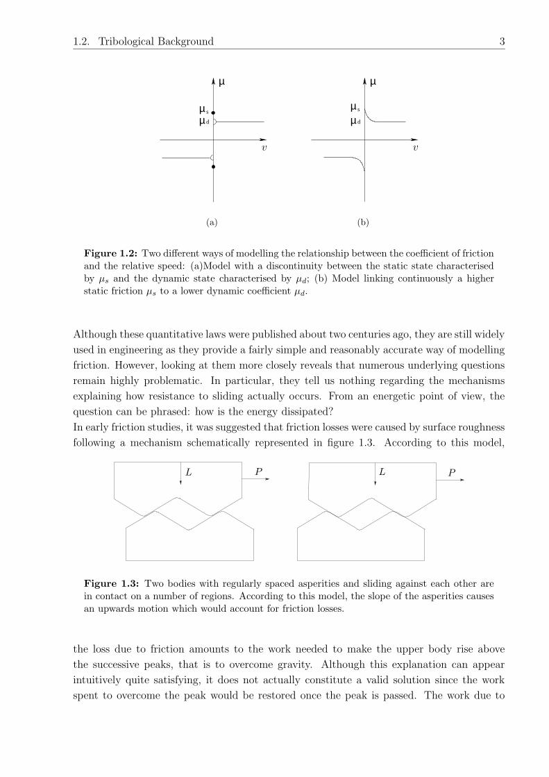
Figure 1.2: Two different ways of modelling the relationship between the coefficient of frictionand the relative speed: (a)Model with a discontinuity between the static state characterisedby µs and the dynamic state characterised by µd; (b) Model linking continuously a higherstatic friction µs to a lower dynamic coefficient µd.
Although these quantitative laws were published about two centuries ago, they are still widely
used in engineering as they provide a fairly simple and reasonably accurate way of modelling
friction. However, looking at them more closely reveals that numerous underlying questions
remain highly problematic. In particular, they tell us nothing regarding the mechanisms
explaining how resistance to sliding actually occurs. From an energetic point of view, the
question can be phrased: how is the energy dissipated?
In early friction studies, it was suggested that friction losses were caused by surface roughness
following a mechanism schematically represented in figure 1.3. According to this model,
PSfrag replacements
P PL L
Figure 1.3: Two bodies with regularly spaced asperities and sliding against each other arein contact on a number of regions. According to this model, the slope of the asperities causesan upwards motion which would account for friction losses.
the loss due to friction amounts to the work needed to make the upper body rise above
the successive peaks, that is to overcome gravity. Although this explanation can appear
intuitively quite satisfying, it does not actually constitute a valid solution since the work
spent to overcome the peak would be restored once the peak is passed. The work due to

4 Chapter 1. A Review Of Literature
friction would then oscillate between a positive and a negative value but on average would be
zero. It was then suggested that friction might be due to asperity plastic deformation: two
peaks in contact would be plastically deformed and this would account for the loss of energy.
Nowadays, it is widely believed that surface deformation (also called ploughing) is indeed an
important source of friction dissipation, but a simple reasoning suggests that it cannot be
the only one: if friction effects were only due to ploughing, the friction force would decrease
as sliding of two bodies is repeated a large number of times: the surfaces would smooth out
leaving smaller and harder asperities to be deformed (due to plastic hardening). In practice,
this is only observed to a very small degree, which means that another phenomenon must be
at work. This new mechanism is called adhesion, according to which the two bodies attract
each other due to short range atomic forces making the two bodies effectively stuck to each
other. Adhesion was already mentioned by Coulomb. However, he ruled it out on the ground
that if this was the actual mechanism,
1. The magnitude of the friction force would increase with the area of contact.
2. Two bodies in contact would stick together even when they are not sliding, and there-
fore, there should be a normal resistance when they are pulled apart.
It was known that neither of these two facts were experimentally observed, at least with
the experimental equipment available at the time. It was only when researchers first made
the distinction between real and apparent area of contact and discovered short range atomic
forces that the idea of adhesion could be considered again as a plausible mechanism for
friction. The work done by Bowden and Tabor (Bowden and Tabor (1956)) is a landmark
in this area.
Adhesion can be explained as follows: real contact only occurs on very small areas (compared
to the apparent area of contact). The size of these areas of contact mainly depends on
the load. Within these small contact zones, junctions between the two bodies are formed.
These junctions, of an unclear “physico-chemical” nature, have both a shear strength and a
traction-compression resistance. The shear strength is at the origin of friction.
A very approximate but simple theory yields some quantitative results. The real area of
contact Ar can be estimated by
Ar =L
p, (1.2)
where L is the load magnitude and p the penetration hardness (the largest compressive stress
that such an area of real contact can carry without plastic yielding). If we assume that when
sliding occurs, the average shear stress over the real area of contact has the value τ , the total
friction force F can be written:
F = τ .Ar. (1.3)
Hence the coefficient of friction
µ =F
L=τ .Ar
p.Ar
=τ
p. (1.4)

1.2. Tribological Background 5
A fair approximation of the average resistance to shear of the junctions constituting the real
area of contact is the bulk shear strength τy of the softer of the contacting materials, so that
µ =τyp. (1.5)
This simple model provides a good explanation of the fact that the coefficient of friction is
independent of the real or apparent area of contact. It also gives some understanding why
the friction force F is proportional to the downward vertical load L.
Formulating friction as a combination of adhesion and deformation satisfactorily explains
many features of friction. In particular, adhesion explains neatly the fact that friction
for two identical, extremely clean metal surfaces can be very high. For then, junctions of
the same nature as those responsible for the cohesion of the material are formed. It also
explains the tribological rule of thumb that it is poor practice to design a contact in which
two like materials slide on one another. In fact, from a statistical analysis of the interface
properties, Greenwood and Williamson (1966) suggested that most friction features could be
explained by adhesion and elastic deformations alone. Although major breakthroughs have
been achieved in the modelling of friction in the last 50 years, many questions are still open.
In 1981, Tabor gave a illuminating review (Tabor (1981)) of these achievements as well as
snapshot of the research situation in the early eighties.
In addition to being a fascinating problem in itself, the conclusion to draw out of this in
relation to brake noise is that although it has been studied for a long time, friction is still
an area of active research where very few questions have a definite answer. In many ways,
the difficulty in modelling friction has an essential role in making the modelling of friction-
induced vibration – including brake noise – a particularly difficult problem.
1.2.2 Background work on friction-induced vibration
In many mechanical systems including a frictional interface, it has been reported that on
some occasions, the relative velocity of the sliding bodies can undergo large fluctuations
under a steady pulling force. The waveform of this oscillation can take various forms but
a close examination often – but not always – reveals that it consists of the alternation of
two distinct phases, namely sticking (no relative motion) and sliding (gross relative motion).
Thus this behaviour is commonly called “stick-slip oscillation”. It seems that in order for
this behaviour to occur, the “right combination” of friction characteristics and structural
elasticity is necessary. Interests in this problem from various areas ranging from bowed
string instruments to machine tool cutting have produced a large and long standing body of
literature, devoted to predicting the conditions under which this oscillation may occur. In
the last decade, Ibrahim (1994a,b) published two very comprehensive review papers on the
subject.
The textbook example used to illustrate stick-slip oscillation is shown in figure 1.4. It has
been the subject of extensive investigations over decades (e.g. Den-Hartog (1933) for an
early example). In most studies, it is assumed first that oscillations do occur. The task is

6 Chapter 1. A Review Of Literature
PSfrag replacements
k
N
V
m
x
F
Figure 1.4: Typical slider on a moving belt system illustrating stick-slip oscillations. A massm attached to the ground via a spring of stiffness k slides on a belt moving at V. The massexerts a downward force N which generate a resisting friction force F .
then to calculate their amplitudes and frequencies (see Bowden and Tabor (1956) p. 105 for
an example of this). Den-Hartog (1933) did not make this assumption and studied separately
cases where there are no, one or two sticking phase(s) of a forced oscillation with Coulomb
friction.
The development of dynamical system theories allowed a more systematic approach to non-
linear problems. In the particular case of the “slider-on-belt”, a dynamical system analysis
can be carried out with fairly simple algebra. To illustrate this, we follow Chambrette and
Jezequel (1992). The friction model used is shown in figure 1.2(a). This model is charac-
terised by a constant coefficient of friction while sliding but a higher value while sticking.
During sliding, the equation of motion is
mx+ kx = F (x− V) = Nµ(x− V). (1.6)
Introducing the following dimensionless variables:
ω2 =k
m; xst =
N
k; τ = ωt; x(τ) =
x(ωt)
xst
; v =Vωxst
, (1.7)
where ω is the natural frequency of the oscillator without damping or friction; xst can be
thought of as non-dimensional static equilibrium position, V0 is the constant velocity of the
belt, and v its non-dimensional form.
The equation of motion can then be rewritten:
x+ x = µ(x− v). (1.8)
The central idea of a dynamical system approach is to get as much information as possible
from the equation itself rather than to struggle to find out a time-parameterised solution.
This information is in general of a geometrical nature and refers to curves in the phase-plane
(x, x). It can be mentioned here that few people have tried to tackle friction problems from
a dynamical systems perspective (see Narayanan and Jayaraman (1989), Popp and Stelter
(1989) and more recently and seriously Ouyang et al. (1999) and Bengisu and Akay (1994))

1.2. Tribological Background 7
Denote the set of initial conditions for the sliding mass m by (x, x), the equation of motion
can take five different forms. In the following list, the equation is stated for each form. Below
the equation is integrated after multiplication by x.
1. Case 1: x < v
x+ x = µd
x2 + (x− µd)2 = x
2 + (x − µd)2
(1.9)
This represents the equation of a circle centered on (µd, 0) passing through (x, x)
2. Case 2: x > v
x+ x = −µd
x2 + (x+ µd)2 = x
2 + (x + µd)2
(1.10)
This represents the equation of a circle centered on (−µd, 0) passing through (x, x).
3. Case 3: x = v and −µs < x < µs
x = −x+ µ = 0
x = x(1.11)
This represents a horizontal line passing x = v.
4. Case 4: x = v and x > µs
x+ x = µd (1.12)
This is a portion of a circle centered on (µd, 0) as in case 1.
5. Case 5: x = v and x < −µs
x+ x = −µd (1.13)
This is a portion of a circle centered on (−µd, 0) as in case 2.
Figure 1.5 summarises the different possible situations.

8 Chapter 1. A Review Of Literature
C
x=+
A
x
ZONE V
B
C
C
ZO
NE
I
ZONE IVZONE III
ZO
NE
II
Γ
µdµsµ− µd−
x.
.x=v
o
o
s
µ
x=−
sµ s
C2
1
Figure 1.5: Phase plane plot showing the different behaviours that a “slider on a belt” systemcan exhibit. Each colour represent a different behaviour.
In summary, the phase plane is divided into 3 different zones. The horizontal line x = v
divides the plane into two regions. Above this line, the trajectories follow portions of circles
centered on the point (−µd, 0). Only one of these is drawn in figure 1.5. These circles are
oriented clockwise. Below the line, the trajectories are circles or portions of circles centered
on (µd, 0), oriented clockwise. The line x = v itself comprises three different regions. Moving
along a circle means sliding, whereas moving along the line x = v means that the mass is
sticking to the moving belt. Let us enumerate all possible cases.
• If the mass starts at point A (i.e. if (x, x) = (µd, 0)), then it remains there forever.
A is a fixed point, the mass is in steady sliding at a fixed position.
• If the initial conditions are such that√
(x − µd)2 + x2 ≤ µs − µd (i.e. if we start
within the circle labelled C in figure 1.5), then the trajectory is a complete circle
centred in (µd, 0). The system behaves like a conservative oscillator. In this case, the
friction force has a constant magnitude and direction, acting like a constant bias on
the elastic restoring force. The system appears as conservative although it has friction:

1.2. Tribological Background 9
the energy fed in the oscillator during the forward motion exactly compensates the
friction loss during backward motion.
• If√
(x − µd)2 + x2 > µs − µd. The initial point can be above or below the line x = v.
Let us assume it is below (the reasoning still holds true if it is above). Then the system
follows the circle of radius√
(x − µd)2 + x2 until it reaches one of the three zones of
the line x = v (labelled zone III or V on the diagram).
– In Zone IV or V, sticking is actually not possible since the elastic force would not
allow it. Therefore, the mass starts sliding in the opposite direction along another
circle. An illustration of this is given on the diagram if we follow first C1 and
then move onto C2. Due to the centre shift between the two classes of circles, the
system will necessarily end up in Zone III after some time.
– In Zone III, the mass actually sticks up to point C where the spring force drags
it back. It then moves on to the portion of circle called Γ. The sliding ends at
point B where it starts sticking again following the same path:
B → C → Γ → B.
This path is therefore an attracting limit cycle and its basin of attraction is the
whole space outside the disc C.
From this, it can be concluded that if µs = µd, then B = C, and there is actually no limit
cycle (i.e. no stick-slip oscillation). This has lead numerous authors (Bowden and Tabor
(1956) for instance) to make spurious logical statements such as “µs 6= µd is a necessary
condition for instability” (sometimes it is claimed to be sufficient...) The origin of this mud-
dle may be the confusion between two levels of “necessity”. Given a set of premises, the
conclusion is necessary provided the rules of calculus/logic are used properly. Whether what
we say about the world is necessarily true is a completely different matter. The answer is
probably no, and this is why experimental validation is necessary. If µs 6= µd is a necessary
and sufficient condition for instability within the model presented above, it does not mean
that µs 6= µd is still necessary if a different model is chosen. In fact, it will appear later that
it is possible to predict instability even with a constant coefficient of friction. And even if
all models exhibited the same necessary condition for instability, it would not necessarily
mean that in reality, instability does occur under this condition (although it would be likely).
The same kind of systematic study can be carried out with a continuous model of friction. In
this case, resolution by hand is not possible and we have to resort to numerical simulations.
Results obtained are somewhat similar as long as the curve µ(vs = x− v) is decreasing. This
condition is again often given as necessary due to the following explanation: in such a system,

10 Chapter 1. A Review Of Literature
∂µ∂vs
< 0 can be interpreted as a negative damping term. Whenever this term overcomes the
positive damping present in the system, then steady sliding is unstable. This line of reasoning
is interesting but it is important not to overstate the scope of its generality.
1.2.3 Normal Degree of Freedom
This work is primarily concerned with brakes as a source of noise. The far field sound
pressure p at position vector r, radiated by a source S at frequency ω is given by the
standard Kirchhoff-Helmoltz integral (Fahy (1985)):
p(r) =1
4πejωt
∫
S
[
p(rS)∂
∂n
(e−jkR
R
)
+ jωρvn(rS)e−jkR
R
]
dS, (1.14)
where p(rS) is the pressure on the surface of the source at position rS, vn is the normal
velocity of the surface, R the distance |r − rS| between the source and the field points.
The integral is taken over the surface of the source in contact with the fluid. Fahi then
adds: “It would seem from equation (1.14) that it would be necessary to specify both the
distributions of surface pressure and surface normal velocity; however, these quantities are
not independent, and the pressure field is everywhere uniquely determined by a specified
distribution of surface velocity on a surface of a given geometry.” The point of recalling this
formula here, is to stress the importance of normal motion for noise radiation. With this in
mind, it remains to find out which parts are vibrating transversely and how such vibration
is generated. The models presented so far now reveal an important limitation: they do not
give any account of transverse motion2. The dynamics is purely tangential. How does this
normal motion then arise?
The first intuitive idea one might have to explain the presence of normal motion is the same
as Coulomb’s (see figure 1.3). In order to overcome each other’s asperities, the surfaces
in contact have to rise and fall successively, causing a normal motion. This is the line
followed by Bengisu and Akay (1998) for instance. Using probabilistic surface models for
two nominally flat surfaces, their friction model sums adhesive and deformative forces over
all asperities. They assume that interface contacts occur at both asperity peaks and on
their slopes. Normal motion originates from these oblique interactions. However it is not
clear whether this type of mechanism with typical engineering surface slopes, is sufficient to
account for the amount of normal vibration observed. As we shall see in the next section,
this normal motion can also be explained by some deformation of the structure itself (Spurr
(1961-1962)). Wherever this normal motion comes from, it is very likely that it has a great
influence on the tangential dynamics. In a seminal paper, Tolstoı (1967) first introduced
this idea. Tolstoı observed that the forward jump movements of a slider during stick-slip
2It seems important to clarify what might appear as a slight semantic drift here. “Normal motion” inKirchhoff-Helmosltz formula means normal to whatever surface is vibrating, whereas “normal motion” inrelation to brake noise means normal relative to the plane of sliding. However, normal to the plane of slidingis also normal to the source, in the Kirchhoff-Helmoltz sense. And it is likely that the normal motion (inboth senses) of a system like the disc plays an important acoustic role in brake noise. So far, it is not clearwhere such a motion might originate from.

1.2. Tribological Background 11
motion occur in strict synchronism with upward normal jumps. Observed decreases of friction
during the sliding portions of the stick-slip motion might thus be the result of a decrease of
the average normal load contact force during the sliding and jumping. This questions the
whole idea that there is an essential difference between static and kinematic friction. And it
implies that any serious attempt at modelling kinematic friction will have to give an account
of the coupling between normal and tangential degrees of freedom. This idea has since been
extensively investigated. For instance Oden and Martins (1985), Martins et al. (1990) as well
as numerous papers co-authored by Hess (Hess and Soom (1991a), Hess and Soom (1991b))
argue that the apparent difference between static and kinematic coefficient of friction can be
explained by the non-linearity of the law governing the contact compliance. This idea will
be further developed in section 4.1. More directly in relation to brake noise, Ouyang et al.
(1999) very recently followed this line of enquiry.
1.2.4 Rock Mechanics Contribution
Much work has been done, based on the slider-on-belt system. The scope of phenomena it
can describe is fairly large. Researchers on geophysics have made a valuable contribution to
this body of literature. One of their interests is to predict seismic dynamics. Carlson and
Langer (1989) modelled two tectonic plates as a train of elastically coupled blocks sliding on
the ground with one of the friction laws given above. With similar objectives, Heslot et al.
(1994) precisely studied both experimentally and theoretically the dynamics of two sheets
of paper sliding over one another. For their theoretical model, they used a very interesting
heuristic approach. Although the problems addressed in these papers have some similarity
with brake noise, the situation differs in some fundamental ways. First, the geometry involved
is completely different. Geophysicists often investigate the dynamic interaction between two
elastic half-spaces (Adams (1995), Martins et al. (1995)). More importantly, the velocities
involved are very low. Lower velocities also implies longer time scales, so that the bodies in
contact can have time to creep, microslip, etc... Many parameters have been suggested to
influence the contact properties: the time of stick, the previous history of a contact zone often
captured through a characteristic length parameter. Rabinovicz (1958) give an interesting
discussion about the intrinsic variables affecting friction.
Closer to brake operating conditions is the oil drilling technique. This problem has become
more acute in the past decades as oil resources have become depleted and consequently
require deeper and deeper wells. The distance between the rotating engine at the top surface
and the drilling head at the bottom is so great that the connecting shaft undergoes large
torsional vibrations. The drill alternatively sticks and slips when the engine rotates at a
constant speed resulting in fatigue problems in the shaft (see Brett (1992)). It is likely
that the friction properties of diamond on rock are quite different from those of a brake
pad on disc which makes these studies only partially relevant, although, in practice, the two
problems can be modelled in a similar way.

12 Chapter 1. A Review Of Literature
1.2.5 Bowed-string vibration
Bowed-string vibration is probably one of the few systems in which self-excited oscillation
is desirable, since it is the source of noise for instruments like violins or cellos. It is also
probably the best understood friction-excited oscillator. Several features make the bowed-
string a system more amenable to analytical treatment. First, the vibration behaviour of a
string is now known in considerable detail, including the modelling of such features as the
slight bending and torsional stiffness of (real) stings. Second, the contact zone is relatively
small and well defined. Most bowed-string instruments only acquire their required musical
properties after the strings have been rubbed with a particular substance called “rosin”.
Rosin is a solid resinous substance obtained by distillation or solvent extraction from various
species of coniferous trees. It has the remarkable property that its glass transition occurs
not far above room temperature, so that it is a brittle and fragile material at ambient
temperature but becomes sticky and starts melting as soon as it is slightly heated up. In
a recent paper, Smith and Woodhouse (2000) studied in detail the frictional behaviour of
rosin in view of understanding its role in the generation of stick-slip oscillations in bowed-
string instruments. They reached several important conclusions. For instance, they gave
convincing evidence that in the system they studied, the usual curve showing the coefficient
of friction decreasing with increasing sliding speed could be misleading because these curves
mostly result from steady-sliding measurements. The frictional behaviour thus described
may not be valid for high frequency velocity oscillation. In these papers, it was also shown
that the most important state variable in the case of rosin was the interface temperature.
The sliding speed was only found to play an secondary role. These conclusions, although
closely tied-up to the particular case of rosin, are worth bearing in mind for any study of
friction-induced vibration.
1.2.6 Concluding Remark
As K. Johnson pointed out in a recent review paper (Johnson (2001)), friction-induced
vibration “is a vast subject, covering extreme ranges of space and time: from seismic faults
stretching many kilometers to crystal lattice spacing in the Atomic Friction Microscope;
from years which separate earthquakes to the kilohertz frequencies of squealing brakes and
railway wheels”. The present section has provided a summary of the key concepts and open
questions in the study of friction-induced vibration. As will be seen in the next section,
many researchers make very little use of these concepts in investigating brake noise. Given
the mechanical complexity of a brake assembly, this is not surprising. However, it is hoped
that this section will help bear in mind the extent and importance of the approximations
made in models discussed next.

1.3. Structural models for brake noise 13
1.3 Structural models for brake noise
Brake noise has been a problem since the emergence of automotive manufacturing. For many
years, a decreasing coefficient of friction with sliding speed was the only way of explaining
how instability could arise in brakes. It was only in the 60s that engineers from the braking
industry suggested that brake noise instability could actually involve the whole structure.
It has been known for a long time that the structure played a key role in this instability.
Anyone who has some practical experience with brakes knows that minor modifications of
the mounting could greatly influence the occurrence of noise. Spurr (1961-1962) was the
first author who proposed a mechanism of an entirely new type, involving a buckling of the
structure itself. From this time, numerous authors tried to extend the idea. Their papers
marked a shift from tribology to structural mechanics.
1.3.1 Sprag-Slip
Sprag-Slip is the name Spurr (1961-1962) gave to the kind of motion his mechanism allowed.
His model is shown in figure 1.6. The rigid strut O′P , pivoted with a circular spring at O′,
PSfrag replacements
L
P
F
O′
θ′θ
O′′
B
V
A
T
Figure 1.6: Example of system exhibiting sprag-slip oscillations. This drawing is a slightlymodified version from the one proposed by Spurr (1961-1962). The mass at P is pivoted tothe strut O′P . The plane AB is moving horizontally at V. There are coil springs at pivotsO′ and O′′. The forces applied on the mass are L, F , T and a reaction from the plane, notshown on the diagram.
is loaded against a moving surface AB at an angle θ. A second rigid strut O′O′′ is pivoted
with a circular spring at O′′. The spring stiffness at O′′ is much larger than that at O′. A
mass m at the end P of O′P creates vertical load L = mg. The strut O′P , pin-jointed at
the top of the mass, exerts an extra force on it at P in the direction O′P . The reaction force
from the ground to the mass compensating the total downwards load is not shown on the
diagram. Newton’s law for this mass, combined with Coulomb’s friction F = µ(L+ T sin θ)
leads to
F =µL
1 − µ tan θ, (1.15)

14 Chapter 1. A Review Of Literature
where µ is the coefficient of friction and θ the angle O′PB.
If O′ is rigidly fixed, F approaches infinity as cot(θ) approaches µ. And when cot(θ) = µ,
the cantilever sprags and motion is impossible.
Flexibility in the pivot O′ is provided by the cantilever O′O′′. When O′P is at the spragging
angle, there is no slip between P and the moving surface AB. In order for motion to continue,
the cantilever O′P is effectively replaced by cantilever O′′P which has an angle θ′ with the
plane AB. θ′ is now smaller than the spragging angle, the value of F falls and slip can occur.
Thus the strut O′P is vibrating. Due to the geometry of the system, the normal force L will
vary as the value of F alters and this will excite transverse modes of the surface AB.
This mechanism highlighted two new features. First, it showed that instability could be
predicted without a coefficient decreasing with increasing sliding speed. In Spurr’s model,
what matters is the actual value of the coefficient of friction. Secondly, it makes clear that the
angle between the rubbing strut and the plane plays a key role, pointing out the importance
of the geometry as a source of instability.
However, this system is still quite far away from a real brake. Researchers who have developed
Spurr’s idea, have progressively refined his approach by bringing the system closer and closer
to a real brake.
1.3.2 Simplified Multiple Degree of Freedom Systems
The first attempt to implement Spurr’s idea in a more realistic model was made by Jarvis
and Mills (1963-64). They studied vibration induced by dry friction on a system comprising
a disc and a cantilever. They draw upon Spurr’s work in that their cantilever represents
the strut O′P in figure 1.6. The moving surface AB is now a disc, allowing some structural
flexibility. The friction force couples the disc and the cantilever at the contact point, (which
implies that they remain in contact). They first considered a coefficient of friction decreasing
linearly with the relative speed, and then kept it constant. Writing Lagrange’s equations
for this system leads to an eigenvalue problem. If an eigenvalue has a positive real part, the
system is unstable: the motion would theoretically grow to infinity. However in practice,
some new mechanisms not taken into account in the model would limit this growth. This
procedure has been used extensively since then. North (1976) gave a useful literature review
of this kind of linear structural approach.
Following the same idea, Earles, with various coworkers, gradually improved the modelling
of a pin-on-disc system for about a decade. In the first paper of the series, Earles and Soar
(1971) successively modelled a pin-on-disc system first taking into account the compressive
mode of the pin then considering its torsion (in fact rotation of the pin with respect to its
mounting arm, see figure 1.7). The braking system is eventually modelled as a two-degree-
of-freedom system. In a subsequent paper, Earles and Soar (1974) adopted an approach
inspired by the early days of the finite element method (the pin was sliced into 5 elements)
and modal analysis: the system is divided into two linear systems (the pin and the disc)
that excite each other at the contact point. This is why they find it useful to use receptance

1.3. Structural models for brake noise 15
PSfrag replacements
x
y
θ
N
N
µNµN
θ + γ
(a) Compressivemodel for the pin.
PSfrag replacements
x y
θ
N
N
µN
µN
θ + γ
(b) Torsionalmodel for the
pin.
Figure 1.7: Diagrams showing 2 degree-of-freedom models. The top mass spring system isthe disc. The bottom mass is the pin with the various degrees of freedom allowed, as shownon each figure.
functions defined at the contact point for each subsystem: β for the pin, γ for the disc. Thus
the receptance of the coupled system α is:
1
α=
1
β+
1
γ. (1.16)
In their 1976 paper Earles and Lee (1976) seem to have returned to the earlier approach of
(Earles and Soar (1971)). The system is still a model of a pin-on-disc but the model now
comprises more degrees of freedom as shown in figure 1.8. As before, in this model only the
PSfrag replacements
DiscPin
xx
y
Figure 1.8: 4 degree-of-freedom model for a pin on disc system. The pin is allowed to rotateand translate vertically and horizontally. The disc is allowed to translate in its transversedirection.
transverse motion of the disc is taken into account. The pin can translate in two directions
and rotate in the plane perpendicular to the disc surface. Then follows an eigenvalue analysis
giving regions of instability when their real part is positive.

16 Chapter 1. A Review Of Literature
In subsequent papers, Earles and Badi (1984) and Earles and Chambers (1988) upgraded
this model by adding a similar pin symmetrically located on the other side of the disc. This
was shown to widen the regions of instability already found with a single pin.
Throughout this series of papers, theory is compared with experimental results obtained on
a pin-on-disc rig. The authors claimed an increasing agreement between the two even though
guessing sensible values for structural parameters such as modal masses and stiffnesses always
proved very difficult.
During the same decade, North (1972) followed a similar line but started with an 8 degree-
of-freedom model shown in figure 1.9.PSfrag replacements
Pad
Disc
Caliper
y0
y1
y2
y3
θ0
θ1
θ2
θ3
Figure 1.9: 8 degree-of-freedom model of a brake assembly after North (1972). The modelcontains 4 rigid bodies: the disc, the caliper and two pads. Each is allowed to move in atransverse direction y and to rotate.
This model comprises 4 parts: two pads, the disc and the caliper. Each of them is allowed to
rotate and to have a transverse motion which makes 8 degrees of freedom. Once again after
the equations of motions are derived, an eigenvalue analysis is carried out leading to some
instability regions. The originality of North is first to suggest that the kind of instability
observed in brakes might be similar to aircraft wing flutter, i.e. a coupling between a rotation
and translation occurring when the two degrees of freedom have a certain phase shift (90
degrees for the wing). Second, he modelled the friction force as a so-called “follower force”.
To illustrate this idea, consider the forces acting on the disc. North considers that the forces
of the pads on the disc are made up of a static compressive preload N0 augmented by an
elastic term depending on the disc-pad separation. For instance, the force exerted by the
top pad on the disc is written:
N1 = N0 +KP1(y0 − y1) + CP1(y0 − y1), (1.17)
where KP1, CP1 are the disc-top pad contact stiffness and damping coefficient respectively
and y0 and y1 the upwards displacement of the disc and top pad (see figure 1.9). With

1.3. Structural models for brake noise 17
similar notations, the force exerted by the bottom pad on the disc is
N2 = N0 −KP2(y0 − y2) − CP2(y0 − y2). (1.18)
The concept of follower force is that the friction force instead of being modelled as remaining
horizontal, is allowed to follow the deflection of the disc – here the rotation θ0. Thus the
friction force on the disc has the vertical component:
Fy = µ(N1 +N2)sin(θ0) ≈ µ(N1 +N2)θ0, (1.19)
and its horizontal component is µ(N1 +N2)cos(θ0) ≈ µ(N1 +N2).
Both ideas of flutter and follower forces have been taken up by numerous authors under differ-
ent forms. It is now widely believed that brake squeal is a manifestation of flutter instability.
The concept of follower forces has become increasingly used by researchers modelling disc
instability caused by a moving load which is the focus of section 1.4.
1.3.3 Systems with extended contact
The system models discussed so far only contained one or two point contacts. However it is
conceivable that there may exist mechanisms of instability intrinsically linked to extended or
multiple contacts (like a brick dragged on a plane, alternatively rocking from front to back
end). For instance, using the finite element method, Hulten (1998) modelled a drum brake
as an in-plane assembly of a drum, a shoe and a lining (relatively compliant layer located
between the shoe and drum). He claims to have identified four different mechanisms causing
instability in drum brakes. Two of these “mechanisms” are due to the curvatures of the shoe
and the drum. This is clearly linked to the extended nature of the line contact.
Along a similar line, Nakai and Yokoi (1996) studied the squealing mechanisms of a band
brake. The band was modelled as a linear flexible element. They observed fairly good agree-
ment between the instability frequencies predicted by linear theory and the noise frequency
measurements. They showed that squeal resulted from the coupling between two modes of
the band.
Rapid increase in computer power in the past twenty years has made it possible to model a
whole brake assembly using the finite element method or multibody dynamics packages. A
number of papers propose this approach (Liles (1989), Ghesquiere (1992), Nack (2000)) with
very similar implementations. The modelling of the individual part is now fairly straight-
forward and many researchers have used the finite element method to get partial modal
information on the system. However modelling the complete system requires the modelling
of the frictional interface. At least up to recently, commercial packages rarely provide an
adequate modelling of this kind of boundary conditions. In all the papers cited above, a
normal compliance spring is included between nodes in frictional contact. The stiffness of
this spring has to be large enough to prevent penetration under normal operating conditions.
The friction force is then applied at the contact nodes. Its magnitude is taken as the product
of the coefficient of friction and the contact spring compressive force.

18 Chapter 1. A Review Of Literature
It seems plausible that the finite element method will eventually be the adequate tool to de-
sign brakes that do not squeal. However, given the lack of understanding of the fundamental
underlying mechanisms at present, the use of FE packages to gain better understanding of
the problem may not be very fruitful, as it adds up its own limitations to an already obscure
phenomenon.
1.4 Loaded disc
In this section, the emphasis is on rotation of the disc. Many papers discussed here were
originally aimed at modelling the problems of circular saw blades or computer disc drives.
Recently, it has been realised that these problems bear strong similarities with brake noise.
Before discussing the influence of an elastic load on a rotor, it seems essential to look carefully
at the vibration of the rotor on its own.
1.4.1 Vibration of a stationary disc
To understand some of the issues associated with the vibration of the brake rotor, it is
convenient to start with a discussion of a particular plate model for this body. Consider
PSfrag replacements
θ
Oreθ
er
Figure 1.10: System of coordinates used to describe the vibration of a static disc.
a uniform circular plate of thickness h, outer radius R and clamped at its center. The
displacement vector u of any point of the disc can be represented as:
u = ur(r, θ, z, t)er + uθ(r, θ, z, t)eθ + uz(r, θ, z, t)ez, (1.20)
where subscripts r, θ, z respectively denote the radial, circumferential and transverse direc-
tion (see figure 1.10). The displacements ur and uθ are known as the in-plane displacements
of the disc. Within the thin plate theory, the out-of-plane displacement uz is supposed to
be independent of z, i.e. uz = uz(r, θ, t).
The problem of transverse vibration of a disc clamped at its centre and free at the periphery
was given a solution within the thin-plate theory more than a century ago. Notably, in “The
Theory of Sound”, Rayleigh (1894, reprint 1945) gave a detailed account of what can be
done analytically on this problem. He showed that the out-of-plane vibration of a disc can
be represented by combinations of radial and diametral modes. The first few of these modes

1.4. Loaded disc 19
are shown diagrammatically in figure 1.11, where the series theoretically goes on to infinity
both downwards and to the right. The equation for the transverse motion uz of a stationary
(2,2)
(0,0) (1,0) (2,0)
(2,1)(1,1)(0,1)
(0,2) (1,2)
Figure 1.11: Diagrammatically mode shapes for the first out-of-plane modes of a disc clampedat the center and free at the outer edge. The first number into brackets is the number of nodaldiameters, the second is the number of nodal circles.
elastic disc is:
ρh∂2uz
∂t2+D∇4uz = 0, (1.21)
where D = Eh3
12(1−σ2)is the flexural rigidity, uz the transverse displacement, ρ the density.
The general solution of equation (1.21) can be written:
uz(r, θ, t) =∞∑
j=0
∞∑
n=0
Wjn(r)Ajn sin(jθ − ψjn) sin(pjnt− φjn) (1.22a)
=∞∑
j=0
∞∑
n=0
Wjn(r)[Bjn sin(jθ) + Cjn cos(jθ)] sin(pjnt− φjn) (1.22b)
where Wjn is a linear combination of Bessel functions whose coefficients are determined by
the boundary conditions, ψjn and φjn are phase angles determined by the initial conditions,
pjn is the set of natural frequencies, and Ajn, Bjn = Ajn cos(ψjn) and Cjn = Ajn sin(ψjn) are
constants.
In the form of equation (1.22b), it appears that for a perfectly axisymmetric disc, each
mode containing at least one nodal diameter is actually a degenerate pair of modes: they
are two different modes that have exactly the same frequency. The two modes of such a

20 Chapter 1. A Review Of Literature
pair have the same number of nodal circles and diameters but the nodal pattern is rotated
so that each nodal diameter of one lies on an anti-nodal line diameter of the other, thus
ensuring orthogonality. There are fundamental reasons for this. The explanation involves
the symmetry groups of the system (i.e. the vibrating system and its boundary conditions).
In particular, one can explain why this degeneracy is always of order 2 and only occurs
for modes with nodal diameters. Murphy et al. (1984a) give an accessible account of this
feature. To give an idea, one can see that for a square plate for instance, there are two
distinct modes with two diameters as shown in figure 1.12. Each nodal system divides the
Figure 1.12: Modes with two nodal lines for a square and a circular plate. The two colorsrepresent a 180 phase shift.
square in different ways so their corresponding modal frequencies will be different. For the
disc, the ’moving mass’ is the same in both cases so the frequencies are indistinguishable. In
practice however, even very slight imperfections prevent most of these doublet modes from
having two strictly identical frequencies. Kim et al. (2000) investigated the influence of the
clamping of the disc on its modal characteristics. They showed that the patterns consisting
of equally spaced bolts on the inner radius interact with the axisymmetry of the disc so that
diameter modes of the perfectly axisymmetric disc will more or less be spatially modulated
by others depending on the symmetry of the bolt arrangement and the characteristics of the
disc. It thus transpires that in practice, even with a static disc, the vibration behaviour can
be substantially more complex than Rayleigh’s description suggests As we shall see in the
next section, the rotation of the disc adds further complications.
1.4.2 Vibration of a rotating disc
When the disc is rotating at a fixed rotation speed Ω, there are two main possible ways
of describing its vibration: either in the frame rotating at Ω, or in a frame “attached”
to the ground. Even if the stresses due to the rotation are significant, it is likely that
the corresponding strains will be small enough so that the dimensions of the rotor can be
considered unchanged. Then one can transform one description into the other using the
transformation:
r′ ≈ r , θ = θ + Ωt (1.23)

1.4. Loaded disc 21
At the beginning of the century, Lamb and Southwell (1921) and Southwell (1921) studied
the problem of the free vibration of a rotating disc clamped at its center. To do so, two
limiting cases were examined. First, the stiffening effect due to rotation was neglected, then
the flexural rigidity was ignored, effectively reducing the plate to a membrane. In both cases
they found that rotation only alters the natural frequencies by a second order correction:
p2 = p2 +BΩ2, (1.24)
where p is the modified frequency, p the frequency of a stationary disc, Ω the rotation
speed and B a coefficient of proportionality. For the first time, it was mentioned that one
could express each mode of a rotating disc as a combination of two travelling waves in the
following way. For a perfect disc ψjn and φjn are arbitrary. One can make them equal
to zero with suitable initial conditions. For each pair (j, n), the term under summation in
equation (1.22a) can be rewritten:
ujn(r, θ, t) =Wjn(r)
2sin (jθ − pjnt) +
Wjn(r)
2sin (jθ + pjnt) (1.25)
where θ = θ + Ωt. This can be interpreted as two travelling waves of shape 12Wjn(r) sin (jθ)
and speed ±pjn/j, moving in opposite direction.
In 1956, Tobias and Arnold (1957) carried an extensive study on the influence of imperfec-
tions on the vibration of a rotating disc. They showed that by combining the sine and cosine
differently in ujn(r, θ, t), it was possible to make the expression look like a combination of
a stationary and a travelling wave or a combination of two travelling waves. In a perfect
disc, the two travelling waves expressed by equation (1.25) have the same frequency and are
arbitrarily positioned in space except that their nodal lines are shifted by π/2j. In practice,
discs are never perfectly axisymmetric. As in the static case, the slightest imperfection ac-
tually fixes the nodal patterns of the modes (the phase angles ψjn are no longer arbitrary)
and splits the two frequencies slightly. The rotation complicates the situation further, since,
as equation (1.24) shows, the frequency of these waves becomes a function of the rotation
speed.
By applying a fixed transverse force (e.g. an air jet) to a rotating disc, one creates a periodic
excitation (whose frequency is the rotation speed). A measurement of the response of the
disc leads to resonance curves, allowing the determination of modal frequencies (this is how
figure 1.13 can be drawn experimentally). For a given mode, there is a value of the rotation
speed which makes the modal frequency equal to zero. This is called the critical speed
(intersection of the lower curve with the horizontal axis in figure 1.13). At this speed, the
undamped response is theoretically unbounded. The disc becomes unstable from the simple
fact that it rotates. This phenomenon has been known for a long time and causes many
problems in rotating circular saws. Studying this problem, Tobias and Arnold (1957) noticed
that the response of the disc actually became non-linear even for very small excitations and
that the pair of modes somehow became phase-locked according to a process which linear

22 Chapter 1. A Review Of Literature
+j
Mod
e Fr
eque
ncie
sCritical Speed
Ω
ΩΩ
Ω−j
2j
+
p
p
j
j
p
+Bjo=p
−
Figure 1.13: Frequency-Speed diagram showing the splitting a mode into a forward andbackward wave.
theory cannot account for. Recently, Chang and Wickert (2001) gave analytical results for
the response of modulated doublet modes to travelling wave excitation. This excitation
was assumed not to be influenced by the response of the disc. They found that depending
on the excitation frequency, the symmetry pattern of potential imperfection and the modal
characteristics of the (“perfect”) disc, various waves either standing or travelling backward or
forward could be predicted. This begins to explain why many researchers using holographic
techniques to observe the behaviour of a brake assembly during squeal come to apparently
contradictory conclusions as for the direction of the travelling waves observed (see section 1.5.
However, by modelling the excitation as an external force, Chang and Wickert only obtained
resonance features. For a more realistic study, it is necessary that both the sliding system
and the rotor be allowed to interact so that the system can become unstable.
1.4.3 Pin-loaded discs
A disc coupled to a moving transverse load has been a subject of investigation for many
years. The problem bears strong similarities with that of a moving load on a beam which
has been used for a long time to model systems such as a train moving on a bridge. They
both involve analysing the interaction between a continuum dynamical system and a moving
oscillator. It is therefore not surprising that similar features appear in both systems: critical
speed, combination resonance...
The typical system studied in this section is shown in figure 1.14. In 1970, investigating the
problem of stability encountered in circular saws, Mote (1970) gave an approximate solution
of the vibration of a disc subjected to a moving load. This solution exhibits resonances for
some values of the rotation speeds (critical speeds). Iwan and Stahl (1973) followed the
same idea but instead of a simple mass, the load consisted of a mass-spring-damper system.
As this was intended to model the recording head on a computer disc drive, no friction (air
bearing) was taken into account. In a fixed frame, the equations amount to an infinite system

1.4. Loaded disc 23
PSfrag replacements
x
y
z
m
k c
Ω
θ
r
r
u(r, t)
Figure 1.14: A stationary disc subjected to a rotating spring-mass-dashpot system loadingthe disc at r. The common transverse displacement of the disc and the mass m is u(r, t).
of coupled linear equations. Solving for a finite set of these leads to an eigenvalue problem.
The influence of various parameters (mass, stiffness...) on the stability can then be studied.
A few years later, Iwan and Moeller (1976) continued in the same line. This time the disc
was moving and centrifugal effects were not neglected. The mass-spring-damper load was
fixed. In both papers, the conclusion was that the load only destabilised the system above
the first critical speed. Mote (1977) examined the problem of a circular saw with floating
central collar (a design innovation at the time). It has a limited relevance to brakes, but
this paper is very interesting for its rigorous mathematical formulation of the problem. In
addition to mass loads, Mote studied the effect of guides. However, any instability found was
again supercritical. Benson and Bogy (1978) carried out similar investigations but modelled
the disc as a membrane. In a series of more recent papers, Yu and Mote (1987), Shen and
Mote (1991a), Shen and Mote (1991b), Shen and Mote (1992), Shen (1993), still working
on discs loaded by mass-spring-damper systems, have gradually developed a different and
more complex approach. Their analysis leads to Matthieu-Hills-type equations known to
undergo so called combination resonances (similar to the pendulum attached to a vertically
oscillating pin). The set of relations relating the frequencies to one another is obtained using
the method of multiple time-scales (Nayfeh and Mook (1979, reprint 1995)). In short, by
identifying the terms of the same order of magnitude in the non-linear equation, several
linear equations can be obtained. Successively solving for these leads to equations similar
to that of “forced oscillators”. Resonances occur when the frequency of the forcing term
is equal to the natural frequency of the homogeneous equation. The type of relationship

24 Chapter 1. A Review Of Literature
obtained is shown below:
(s− l)Ω = prs − pkl, (s+ l)Ω = prs − pkl (1.26)
where r, k is the disc mode under consideration, Ω is the rotation speed (of the disc or the
oscillation depending on the case) and s and l are any two integers such that s > 0 and
l ≥ 0.
1.4.4 Loaded disc with friction force.
Following Iwan and Stahl (1973) and Benson and Bogy (1978), Ono et al. (1991) were still
interested in addressing the hard disc drive stability issue. The disc was modelled as an
elastic plate. Centrifugal forces were taken into account. The slider was made of two heads
rubbing on each side of the disc. They were allowed to move transversely and to roll about
the centre of gravity of the pair of heads thus following the deflection of the disc. The system
being symmetrical, this centre is located on the median plane of the disc (pitch motion). No
motion of the slider in the plane of the disc was allowed. The head was supported vertically
by a spring-damper system. The friction force was taken as equal to 2µFz where Fz is the
transverse reacting force between disc and slider. They solved the equation by trying a
solution of the form:
u =L∑
l=0
Gl(r, t) cos (lθ) +Kl(r, t) sin (lθ), (1.27)
where L is the number of modes chosen.
The stability of the system was given by the eigenvalue real parts. By varying various
parameters, they showed that the friction force actually destabilises any increasing frequency
wave while it stabilises any wave whose frequency decreases with the rotating speed (see
figure 1.13). Although the introduction of friction was a new feature, this paper, dealing
with very flexible discs and fairly high rotation speeds is of limited interest for the study of
brake noise. Combining Ono et al. (1991) and Mote’s ideas, Chan et al. (1994) were able
to predict combination resonances for a load spinning on a disc with friction. Ono et al.
(1991) and Chan et al. (1994) were innovative in that they explicitly used the concept of
the so-called ‘follower forces’ for the first time. The underlying idea is that the slider force
actually follows the deflection of the disc (both in pitch and transverse motion). Figure 1.15
represents such a system. They concluded that the friction force destabilises all forward
waves whereas all backwards waves are stabilised. This is similar to the conclusions reached
by Ono et al. (1991). At the end of the paper, Chan et al. (1994) carried out a cross-check,
solving the same model using a state-space method. This consists in casting the equations
into a matrix differential system and then computing the eigenvalues. It was claimed that
both methods agreed fairly well. Both in Ono et al. (1991) and in Chan et al. (1994) friction
is shown to induce instability below the critical speed.
The finite element method enabled Mottershead et al. (1997) and Mottershead and Chan
(1995) to model a system much closer to a brake assembly: an elastic pad loaded a disc

1.4. Loaded disc 25
PSfrag replacements
Deformed portion
Undeformed portion of the disc rim
Fθ
Fθ
Fz
Fz
h
m
k
c
z
rdθ
u + duu
Fθ∂ur∂θ
rθ
Figure 1.15: Mass-spring-damper system loading a disc with a follower friction force. Theinnovative feature of this model is to allow the friction force Fθ to follow the disc deflexion i.e.to take into account Fθ
∂ur∂θ in the vertical direction.
over a finite distributed area. Their analysis showed that each doublet mode is amenable to
flutter if the pressure load is sufficiently high. According to them, flutter arises from a phase
locking of the modes of a doublet. This idea will be further discussed in the next sections.
Tseng and Wickert (1998) also studied the stability of a rotating disk loaded over an angular
sector. The load was treated as a nonconservative follower type. Shear stress in the disc was
also taken into account. Using the finite element method, they predicted unstable modes
and reached interesting conclusions regarding travelling waves.
In a recent paper, Ouyang et al. (1998) returned to a point load but added several new
ingredients to it. First the friction law was linearly decreasing with the relative sliding ve-
locity. Second, the load had an in-plane spring-dashpot in addition to the previous transverse
one. The analysis is again carried out using the method of multiple time-scales. The intro-
duction of an in-plane spring-dashpot and a negative friction-velocity relationship is shown
to stabilise some otherwise unstable existing modes but their presence was also shown to
create new combination resonances. Over the past decade some researchers have suggested
that in-plane modes of the disc could play an important role in the occurrence of brake
noise. However these suggestions were based on purely experimental observations and to our
knowledge, no proper investigation into the subject has been published so far. Admittedly,
in-plane modes of the disc are likely to be excited by the friction force. However it is difficult

26 Chapter 1. A Review Of Literature
to reach any conclusion regarding their potential role in destabilising the system without a
more careful study.
In summary, parametric resonances are a way of accounting for instabilities in disc brakes,
where the disc rotates past a stationary pad. When friction is introduced, subcritical in-
stabilities can occur; this correlates with the fact that brake squeal can happen at very low
speeds. However, none of the recent papers dealing with parametric resonances actually
proposes any experimental investigation to verify their findings. A considerable amount of
experimental work has been done on braking systems though. This is the subject of the next
section.
1.5 Experimental studies
So far little has been said on experimental studies carried out on brake noise. Although
it has only been mentioned briefly, many of the papers listed in the section “Structural
Models” report experimental testing (Earles or Jarvis for instance). These experimental
investigations are usually on a rig designed to represent the theoretical model (most of
the time a pin on disc system). Some valuable experimental work has also been done on
real brake assemblies. This research can be divided into two main categories. First are
mainly tribological observations, investigating the details of the interaction between pad
and disc in operating conditions. Second are the vibration-based experimental studies. Into
the latter category comes a set of MIRA papers, which reports a whole collection of general
experimental observations made on real brake assemblies. Some researchers have also tried to
achieve some understanding of brake noise by studying the vibration behaviour in operating
conditions using laser holography. A brief account of this will be given next. Finally, a
number of researchers have looked at different experimental aspects of operating brakes.
Usually, a theoretical point is considered, then a set of experiments, devised to verify it, is
carried out. These will be considered under the heading “Semi-experimental work”.
1.5.1 Tribological properties of the disc-pad interface
Eriksson and Jacobson from Uppsala University have carried out a number of experiments to
gain information on the tribological behaviour at the interface between the brake pad and the
disc. Two main concerns inspired their research. First to describe in detail what occurs at the
interface during operating conditions (Eriksson and Jacobson (2000), Eriksson et al. (2002)).
They found that the surface profile of the pad changes significantly within a short time scale.
Contact between the pad and the disc occurs mainly around the steel fibers of the pad, around
which wear debris accumulate, forming contact plateaux. Contact shifts from one plateau to
the next as the steel fiber serving as an anchor is itself worn. Their second concern was to
correlate this detailed tribological behaviour with the occurrence of squeal (Bergman et al.

1.5. Experimental studies 27
(1999), Eriksson and Jacobson (2001). By conducting a large number of braking tests on
well controlled brake assemblies, they concluded that the coefficient of friction increases as
more and more brakings are applied. This increase in coefficient of friction is also correlated
to an increase in squeal occurrences. For the systems they investigated, they found that
a threshold value for the coefficient of friction existed under which very few squeal events
occurs whereas they were numerous above. This is reminiscent of many other studies (Oden
and Martins (1985), Spurr (1961-1962)).
1.5.2 Vibration-based experiments
“Classical” Experimental Work
In the late fifties, R. A. C. Fosberry and Z. Holubecki carried out an extensive experimental
program on real brake assemblies. The first three of these are concerned with drum brakes.
In the first, Fosberry and Holubecki (1955) report very interesting observations on possible
mechanisms of squeal and on their potential causative factors. At that time, the main
reason for squeal was thought to be the negative slope of the friction-speed curve. They
found experimentally that a brake was indeed more prone to squeal whenever the torque
time history presented an “overshoot” shortly before the rotation has completely stopped
(see figure 1.16) This suggests that squeal does not necessarily arise from a static coefficient
Torque
Time
(a) Squealing
Time
Torque
(b) Not squealing
Figure 1.16: Plots showing the variation of the braking torque during stopping tests – afterFosberry and Holubecki (1955)
of friction higher than a dynamic one but rather from a sudden increase of the dynamic
coefficient of friction when the speed is close to zero. They noticed that squeal frequencies
do not usually coincide with any of the natural frequencies of the parts, except when a
special short lining was used (instead of the full-length lining used in real drum brakes,
they tried some short samples of these, shorter but still with the same width as the drum).
However, when the natural frequency of the drum was lowered by addition of masses, squeal
frequencies were also lowered. It might be argued that the natural frequency of the parts of
the brake may be different when brake pressure is applied. If the squeal frequency was among

28 Chapter 1. A Review Of Literature
some of the natural frequencies of the brake in an operating state, it would be expected that
squeal be affected by the brake line pressure. Experiments showed that this was not the
case at a standard level of accuracy (more precise measurements revealed that the squeal
frequency follows the pressure variation but to a much lesser extent : 0.0025% of variation).
Many observations tend to prove that the higher the contact pressure, the higher the squeal
frequency. And indeed, improving the shoe-drum contact by increasing the shoe flexibility
tend to shift the squeal frequency up although the result is not systematic. Although some
tangential vibration was observed at or near squeal frequencies, the noise is thought to come
from some normal vibration (excited by the tangential one). More precisely, they concluded
that a high frequency squeal was primarily due to drum vibration, low frequency squeal due
to back-plate or shoe vibration and groan or hum to suspension/mounting resonance (all of
these originating in tangential motion). In general, it is possible to “locate” a squeal by the
following set of parameters : line pressure, lining temperature, rotation speed. Temperature
was shown to play an important role in the occurrence of squeal. General features such as
intermittency, inconsistency and unpredictability, known for a long time, are also recalled.
The second report (Fosberry and Holubecki (1957a)) explained the phases of development
of a damper for heavy vehicle drum brakes. The principle is to make the drum run against a
collar and thus dissipate vibrational energy by friction. The system is claimed to be effective
and has been patented.
In the third report, Fosberry and Holubecki (1957b) carried on with another kind of damper,
this time acting on the shoe. The second part of the report is a collection of observations on
factors affecting squeal. Here are some of them.
• The squeal is more prevalent at low temperatures (about 100C) but a strange and
important feature of squeal is that its occurrence depends on the thermal history of the
lining: it was noticed that a brake was much more likely to squeal if it had been heated up
to 200C (through operating the brake) and cooled down several times before.
• A minimum line pressure was required before squeal could be obtained. It was no-
ticed, however, that as line pressure was increased, there was a tendency for the normal high
frequency drum squeal to predominate. The state of running-in of the lining was another
factor found to influence squeal. It was found that squeal could be excited by a small piece
of lining, only manually pressed against the drum. Thus, they suggested that local high
pressures are sufficient to lead to squeal.
The fourth and fifth reports (Fosberry and Holubecki (1959), Fosberry and Holubecki (1961))
follow a similar line but deal with disc brakes. It was already suggested in previous reports
that while squealing, the drum vibration was similar to that of a bell (for a theoretical insight
into bell vibration see Perrin and Charnley (1973) and Murphy et al. (1984b)). Trying to
locate the nodes and antinodes of the vibrating modes, they found that the shoe seemed to
be always located at a nodal line of the drum. However, as results were difficult to interpret
(especially with full-length linings), they suggested that the nodal pattern may actually be
rotating, (or be a combination of rotating and static patterns). The same kind of questions

1.5. Experimental studies 29
were posed again for disc brakes, (Tobias and Arnold (1957) were working on the same
issues from a slightly different perspective at roughly the same time.) They tried to locate
the nodal patterns for a few modes. With a steady squeal, the nodes and antinodes could
be detected by moving a vibration pick-up around the disc and noting the changes of phase.
Measurements were made both with the brake squealing and with the brake stationary. In
the latter case, the disc was excited by a shaker acting axially near the disc edge. The nodal
pattern near the friction pad proved very difficult to obtain. By completion of the visible
nodal lines, they came to the conclusion that for a supposed 8 diameter mode, two nodes
would be expected in the pad region. Thus the pad center was found to be approximately
at an antinode, i.e., at a region where the principal motion is axial. Later measurements
confirmed large axial motion there. This finding is in contrast with the drum brake vibration
where the specimen was at a node for radial motion of the drum, i.e. at a position where
tangential movements take place in the direction of the drum (which could satisfactorily
explain the coupling between tangential and normal motion as for a finger sliding on a glass
rim). In their last paper they returned to this question and changed their conclusions. They
eventually concluded that the completion of the nodal pattern was wrong and what was
thought to be an 8 diameter mode turned out to be a 6 diameter mode with uneven spacing:
two nodal sectors conflated in the pad region where all points were found in phase. This
conflation of two nodal sectors into one was also found for other modes.
Measurements of the amplitude of vibration at different parts of the brake showed that vi-
bration was largely confined to the disc and calliper assembly with a maximum amplitude
of vibration in an axial direction on the disc. The method of mounting of the brake sus-
pension and calliper did not affect the measurements. At the end of each report a set of
recommendations aimed at preventing squeal are given, in light of the observations made.
Laser Interferometry
In the early eighties, the development of laser interferometry had become wide-spread enough
to be applied to problems such as brake noise. The main advantage of this method is
that it allows a visualisation of the system while operating (which is very difficult with
accelerometers). Fleske et al. (1978) were among the first to give a complete set of pictures
of various disc-brake parts using this method. These pictures were shot while the disc was
being artificially excited at squealing frequencies. Their pictures show that a nodal line of
the disc is always located in the middle of the pad (see figure 1.17).
They also concluded that the main source of noise was the calliper and not the disc. Albeit
surprising, other more recent studies arrived at the same conclusion (Talbot and Fieldhouse
(2002), Auweraer et al. (2002)).
A few years later, they carried out similar investigations on a drum brake (Fleske et al.
(1980)). They concluded that vibration modes of the drum were insignificant regarding
squeal, at least for low squeal frequencies. They concluded that around 1kHz, the noise is
mainly due to back-plate vibration.

30 Chapter 1. A Review Of Literature
Disc
Nodal linePad
Figure 1.17: Nodal line of the disc passing through the middle of the pad (other nodal linesnot shown)
“Semi-experimental” work
In the early eighties, Lang and Smales (1983) marks the start of a series of papers explicitly
aimed at bridging the gap between the numerous pin-on-disc models that appeared in the
seventies (c.f. Earles...), which were criticised for being too remotely related to real brakes,
and the purely empirical studies providing ‘fixes’ to brake noise, with very limited success.
A list of noises encountered in brakes was given and for each of them, a mechanism is
suggested, reflecting the state of knowledge at the time. The paper then takes the form of a
manifesto giving guidelines on how, according to the authors, the brake noise problem should
be tackled. Six years later, Lang and Newcomb (1989) described experiments carried out on
commercial vehicle drum brakes. Their measurement technique was innovative in that they
managed to attach accelerometers to the rotating drum. Thus a record of the vibration in
a frame fixed to the rotor could be obtained. A reference accelerometer was positioned at
the leading end of the shoe platform so that transfer functions could be measured. Taking
measurements at various angular positions, they obtained the waterfall chart reproduced in
the left plot of figure 1.18. From these, they concluded that the drum mode (fifth order) is
stationary in space and not rotating with the drum. However, a comparison with the mode
shape obtained by impact on a stationary brake revealed important differences. When the
drum is rotating, the wave amplitude never goes to zero (no real nodes are present). This
is visible in figure 1.19, left. A few remarks can be made on their conclusions. First, the
pictures presented here reproduce those of the paper. In particular, it is not clear why when
the range [0 − 180] is labelled “one revolution” (should not it be [0 − 360]?). Second, the
waterfall chart clearly shows that the amplitude at a fixed point on the drum is not constant.
But the only conclusion that can be drawn from this observation is that the nodal pattern
does not rotate with the drum. Claiming that it is not rotating at all (i.e. stationary),
is unjustified and the comparison with the theoretical fixed mode shape (figure 1.19 right)
tends to prove that it is wrong.
They then suggested that the waveform observed with rotation was actually the superposition
of two identical fifth order modes displaced both spatially and temporally from each other (an

1.5. Experimental studies 31
180
Harmonic
Squeal frequnency
Am
plitu
de
Frequency
o90
o
Ang
ular
pos
ition
(a) Amplitude waterfall chart.
180
Phas
e (D
eg)
−
Angular position (DEG) 180 0
o180
o
0
(b) Phrase profile at squealing frequency.
Figure 1.18: Transfer function data measured on the drum brake at various positions aroundthe rotating drum – after Lang and Newcomb (1989).
Angular Position (Deg)
T,.
F. A
mpl
itude
00 180
5
One Revolution
(a) Experimental amplitudeprofile at the squeal frequency.
One Revolution
The
oret
ical
Pha
se
−180
180
0
The
oret
ical
Am
plitu
de
(b) Theoretical phase and amplitudefor a fifth order mode.
Figure 1.19: Comparison of the measured mode shape at squeal frequency and its theoreticalshape.
idea which may have been inspired by the flutter interpretation introduced by North (1972)).
They claimed that this is justified by the fact that the experimental transfer function can
be represented by a real mode and an imaginary one, both stationary in space (with respect
to the ground), with different amplitudes and time shifted by 90. The result of such a
decomposition is shown in figure 1.20. Based on the assumption that the noise comes from
the presence of this pair of modes, “fixes” are suggested (by the addition of masses at some
appropriate positions, aimed at making the drum modes stationary).
Some interesting ideas are presented in this paper however some of the conclusions arrived

32 Chapter 1. A Review Of Literature
180
Am
plitu
de
0Revolution
Real Part
o0
o
Imaginary Part
Figure 1.20: Real and imaginary components of drum squeal mode. The (red) dashed lineis the real part. The solid (blue) line is the imaginary part. According to Lang and Newcomb(1989), the combination of these two components into an amplitude explains 1.19(a).
would need some qualification. In the appendix of their third report, Fosberry and Holubecki
(1957b) suggested that the waveform could be made of a static component (with the ground)
and a rotating one (not necessarily at the drum speed). That seems plausible enough and
in any case should not be ruled out without any consideration.
On the occasion of a conference on “braking of road vehicles” in 1993, the same group
of authors published a few papers drawing upon their previous work. Lang et al. (1993)
examined the influence of rotor geometry. In a the first part of the paper, they gave some
experimental facts in relation to “mode locking”. A brief explanation of this term seems
appropriate at this point. Each part of a brake assembly has its own set of natural frequencies.
It can happen that when two frequencies of two different parts are close, once assembled,
they couple together to form a single mode. A currently popular method, which has had
some success, is to try to eliminate coincident frequencies by structural modifications –
the assumption being that squeal occurs at such coincident frequencies. In practice such a
criterion is not as useful as it might first seem since among all the modal frequencies of all
the parts of a brake there are bound to be many with coincident or close modal frequencies.
The difficulty is then to predict which of these are actually squealing (and why).
However Lang et al. (1993) seemed to undermine this assumption by noticing that if the
brake squeals at a frequency close to a free mode of a part, the shape of the coupled mode is
actually different from that of the original one: the squeal is at 580 Hz, which is close to the
570 Hz first torsional mode of the shoe. But, it turns out that under braking conditions, the
mode shape of the shoe at 580 Hz involves very little torsion of the shoe. They suggested
that this was so because the modal frequencies of the free parts were probably very different
from those of the same parts when the brake is actuated. A modal analysis of the drum
when pressure is applied was therefore carried out. This revealed that the drum had now
several modes of identical shape (n=2, s=0) around the squeal frequency, only differing by
a rotation3 . Concluding that a modal analysis of part of the brake (either actuated or
3Note that under braking conditions, the drum is only one part of the whole coupled system, so that

1.5. Experimental studies 33
not) was not very useful, they carried out a modal testing of some parts of the brake in
squealing conditions. An experimental technique similar to that of Lang and Smales (1983)
allowed a measurement of the mode shape of the rotating drum as well as that of the shoes.
Using North’s flutter model, they showed that the splitting of the frequencies of two identical
modes could have a stabilising effect. It was then suggested that the addition of mass could
artificially split doublet modes and possibly reduce the occurrence of squeal. The purpose of
the masses was to “attach” the mode shapes to the drum so as to stop them from fluttering.
However they never seem to mention the possible “clamping” of the waveform due to the
application of pressure. If a mass can modify the wave motion, surely the influence of the
brake line pressure probably interferes in some way too?
Fieldhouse and Newcomb (1993) asked similar questions, but they worked on a disc brake
and used holography (a few years later Fieldhouse and Rennison (1996) used holography
as well to study drum brakes). Their first objective was to determine whether the nodal
pattern was moving or not. To answer this, they took successive pictures of the disc with
very short time intervals. From this, they concluded that the nodal pattern was moving with
respect to both the disc and the ground and, even more interestingly, the rotation speed of
the nodes was amazingly close to the squeal frequency divided by the number of diameters,
which recalls the critical speed value encountered many times in the “loaded disc” section.
This appears to contradict the common observation that there is a nodal line at the middle
of the pad. However, it might be noted that for an 8 diameter mode, the pad motion is
probably more complex than the rigid rocking assumed for the flutter model and observed
by Lang and Smales (1983) for a low frequency squeal (580Hz).
In the second part of the paper, their interest shifts to the investigation of the influence of
a wire located at various positions between the piston and the pad back plate. By doing
this, they intended to test the validity of the sprag-slip theory (Spurr (1961-1962)). The
layout of the rig is schematically described in figure 1.21. For each wire position, the testing
procedure was to increase the disc surface temperature to over 150C and then to vary the
system pressure from 1 MPa down to zero and then back up to 1 MPa. The temperature was
then allowed to fall to 10C and the process repeated again. The test variables were therefore
the wire offset, the disc surface temperature, and the system pressure. The measured results
were the frequency of the noise generated, the amplitude and the duration. As the data
was somewhat erratic (intermittent, complex frequency content...), the parameters recorded
were combined into a kind of averaging formula devised to grasp the essential features of
the noises and allow for their comparison. The influence of each parameter was examined in
turn. The results showed that for some offset positions ([+12mm, +15mm]), the brake was
readily noisy regardless of the operating conditions (temperature, pressure). This was called
“bad design instability”. When the system was less systematically unstable, the influence of
temperature and pressure on the occurrence of squeal was much more visible, revealing that
different mechanisms may be competing. They observed that decreasing the temperature
it is possible that the drum has a similar mode shape for a few different frequencies without violating theorthogonality requirement.

34 Chapter 1. A Review Of Literature
Backing PlatePiston
Calliper Fingers
Finger Pad
LeadingTrailing
Disc Rotation
Offset
Zoom on the wire
Wire
Disc
Piston Pad
Figure 1.21: Diagram of the set up used by Lang and Smales (1983) to investigate theinfluence on stability of the position of the wire located between piston and pad
makes the brake more noisy. In relation to temperature, it is interesting to note that the
pad coefficient of friction rises from 0.38 at 100C up to 0.43 at 50C. The conclusion is as
clear for the influence of pressure. This allows them to define various stability domains:
1. A domain labelled “unstable” where the brake has a high propensity to generate noise
due to bad design.
2. A “conditionally stable” domain where the brake is normally stable except for some
particular operating conditions.
3. A “stable” domain in which the system is stable regardless of the operating parameters.
This is summarised in the diagram shown in figure 1.22.
oC
Increasing µ
TemperatureEffects
EffectsPressure
EffectsFrictional
Max
Stable
Decreasing P
Unstable
Conditionally Stable
Figure 1.22: Domains of Stability concluding the study by Lang and Smales (1983)
Finally, Brooks et al. (1993) applied an eigenvalue sensitivity analysis to a 12 degree-of-
freedom lumped-mass model. The model – representing a disc brake – is very similar to
that of North (1972) (see figure 1.9). A sensitivity analysis of a function simply consists in

1.6. Conclusion and outline of the dissertation 35
computing the partial derivative of this function with respect to each parameter. A large
derivative with respect to parameter p, at a given point in the parameter space, indicates
that the function is very sensitive to p (a small variation of the p induces a large variation
of the function) and similarly a small partial derivative with respect to p indicates a small
sensitivity to p. Although the principle is certainly not new, it had never been applied to
brakes before and, furthermore, their conclusions were interesting (although the scope of
their generality is obviously tied up to the model considered). From their study, it appears
that the critical parameters for the eigenvalues to have a positive real part are:
(1) the length of the pad,
(2) the pressure application point and
(3) the absolute value of the friction coefficient.
This correlates with many recent findings. This type of analysis seems to be a good com-
plement to lumped-mass models. These have been criticised many times for being difficult
to relate to real brakes. It is indeed very difficult to know in practice what value should
be given to spring stiffnesses or damper constants. One can never be sure that the model
would not have exhibited a different behaviour if different values had been used. This can
be formulated in a more abstract way: sensitivity analysis is a simple route to address the
question of structural stability, how does the solution change when the differential system is
slightly modified?
The papers discussed in this section contain many interesting ideas and one can but approve
of the overall objective of relating theoretical conclusions more closely to experimental obser-
vations on real brakes. However they tend to lack a theoretical unifying basis: all too often
the only outcome is a list of fragmented and apparently sometimes contradictory empirical
observations. This is particularly visible on the travelling wave issue: Chang and Wickert
(2001)’s theoretical approach provides clear predictions and could therefore be used as a
sound underlying basis for experimental testing.
1.6 Conclusion and outline of the dissertation
The large amount of literature produced on brake noise, as well as the variety of the type of
modelling used are a clear indication of the difficulty in explaining and reducing brake noise.
To date, there is still very little agreement on the mechanism(s) underlying the phenomenon,
beyond the fairly obvious statement that noise results from the interaction between friction
and structural characteristics of the system. It is also striking that very few researchers give
a clear justification for the choice of modelling adopted. To help identify the limitations of
the literature published as well as put into context the work presented in this dissertation,
it is useful to cast the papers reviewed according to a series of basic contrasts:
(1) Generality/Specificity. Despite the variety of models proposed in the literature,
most of them have in common that they are tied to some specific experimental apparatus
(either a whole brake assembly or some simplified version of it). This makes it particularly

36 Chapter 1. A Review Of Literature
difficult to assess whether the conclusions reached can be applied to other systems or not.
On the other hand, the widespread occurrence of friction-induced noise seems to call for
a more general approach. Some researchers have proposed more general theories for brake
noise (e.g. Nishiwaki (1993)). However this type of modelling is so ambitious that it is hard
to see how it could be experimentally tested.
(2)Incipient noise/Fully developed noise. In principle, modelling the vibration of
a brake assembly in its fully developed regime would be ideal. However, it may be possible
to satisfy the needs of brake manufacturers without going so far. Their primary interest
seems to be to identify at an early stage of design, whether a particular brake is going to
squeal or not. To understand how squeal actually develops might not be necessary. This
latter opposition is closely related to the next.
(3) Linear/Nonlinear models. It seems plausible that in practice, a growing insta-
bility remains bounded due to some nonlinearity of the system. It is difficult to know a
priori which non-linearity/ies will come into play. They might be specific to each particular
system at a given time. If this is so, researchers using holographic or other experimental
techniques for the investigation of fully developed noise most probably actually study a non-
linear phenomenon. On the other hand, many models (especially those listed in section (1.3))
are linear. Presumably, one can only expect them to predict the noise characteristics at an
incipient stage.
In the work presented here, the choice for each alternative has been made so as to keep the
overall project consistent. The modelling will apply to a whole class of different systems but
the analysis remains strictly within the bounds of linear theory. Therefore, the experimental
testing will primarily focus on the noise at its incipient stage. The overall objective of the
dissertation is to provide a critical assessment of the appropriateness of linear theory for the
study of brake noise. Ultimately, the question which is to be answered is: “How much can
a linear model predict of brake noise?”
In Chapter 2, a linear model of a pin-on-disc system will be presented. This model can be
thought of as the simplest of the models presented in section 1.3. It nevertheless exhibits
many features found in more complicated models and will serve as an interesting case study
for the more general model presented in chapter 3.
Chapter 3 is the fundamental theoretical chapter of the thesis. It contains the general
formulation of instability induced by dry friction between two linear systems in contact at a
single point. The friction law at the contact point features a constant coefficient of friction.
The predictions of the theory will be illustrated by simulated cases.
In Chapter 4, various ways of extending the model presented in Chapter 3 will be investigated.
These extensions all fall within the scope of linear theory. Particular emphasis will be laid on
(1) the influence of compliance at the contact point, (2) the effect of a coefficient of friction
varying with sliding speed; (3) the influence of non proportional damping in the structure

1.6. Conclusion and outline of the dissertation 37
will also be discussed.
Chapter 5 will report results from the experimental testing carried out. A rig was specially
designed to test the theory presented in Chapter 3. After a description and some justifications
for its design, results will be discussed.
Finally, chapter 6 presents the conclusions emerging from this study and gives some directions
for further research.

38 Chapter 1. A Review Of Literature

Chapter 2
Study of a pin-on-disclumped-parameter model
2.1 Introduction
The idea underlying the simulations presented in this section originates from the commu-
nication that J. D. C. Crisp made to Jarvis and Mills’s paper (Jarvis and Mills (1963-64)),
where he argued that the model the authors proposed was unnecessarily complicated. He
suggested a simpler two-degree-of-freedom model supposed to preserve the features of the
original one. Despite the simplicity of the models, the simulations presented in this chapter
give a more precise idea about the main characteristics and limitations of a lumped-mass
model. This model will also be used in the following chapter as the basis of a simple case
study.
The two models studied here are part of the family of pin-on-disc models. From the modelling
point of view, this means that the contact zone is so small that it can be assumed to be a
point. Pin-on-disc systems also have the advantage of bringing to the fore the importance
of the angle between the pin and the disc for the stability of the system – a feature which
will receive closer attention in the following chapter. For each model, the general properties
of the undamped model are studied first, then the influence of damping is discussed.
2.2 Two degree-of-freedom model
This first model is the simplest conceivable model of a brake assembly. Following Crisp
(Jarvis and Mills (1963-64)), only two degrees of freedom are taken into account: the trans-
verse motion of the disc and the fundamental bending mode of the pin. This kind of modelling
is sometimes called a lumped-parameter model because it proceeds by replacing the details
of a mode by an equivalent discrete mass-spring-damper system. The pin has a variable
inclination angle θ with respect to the disc normal. This is summarised in figure 2.1. The
friction law used for the coupling between the friction force F and the normal force N at the
contact point is represented in figure 2.2. It is Coulomb’s law with a constant coefficient of
friction µ.
39

40 Chapter 2. Study of a pin-on-disc lumped-parameter modelPSfrag replacements
mf
Md
kf
Kd
FN
Vu
w
θ
Disc Rotation
Pin
Disc
(a) Physical system
PSfrag replacements
mf
Md
kf
Kd
FN
V
u
w
θ
Disc Rotation
Pin
Disc
(b) Mathematical model
Figure 2.1: Two degree-of-freedom model: N and F are the normal and friction forcesrespectively. They are drawn as acting on the pin in the figure. mf and kf are the mass andstiffness for the fundamental bending mode of the pin. Similar notations are used for the disc.u and w are the transverse displacements of the pin and the disc respectively V is the discrotation speed.
PSfrag replacements
µ
µ
−µ−v
−V vrelat
Figure 2.2: Friction law used for the model. V is the disc speed. µ is the constant value ofthe coefficient of friction.
The pin mode is characterised by a mass, stiffness, and damping constant mf , kf , cf respec-
tively. The subscript “f” stands for flexure. Similarly, the disc modal properties are denoted
Md, Kd, Cd (capital letters and subscript “d” for disc). The transverse displacement of the
pin is u. That of the disc is w. Their orientation is as shown on figure 2.1. The dampers
are not shown on the figures to prevent overloading. A normal preload N was introduced
in order to keep the total normal force positive (a negative normal force would mean loss of
contact).
Throughout this chapter, the parameter values used are:

2.2. Two degree-of-freedom model 41
Disc Frequency: 30 Hz
Disc Modal Mass : 1 kg
Disc Damping Ratio: 0.005 (where applicable)
Pin Bending Frequency: 20 Hz
Pin Bending Modal Mass : 0.1 kg
Pin Bending Damping Ratio: 0.01 (where applicable)
Disc Speed V = 0.4 m/s
Normal Preload N = 10 N
Coefficient of Friction µ = 0.5 or 0.7
Initial conditions:
u = 0 m/s
u = 10−4 m
The case without damping is considered first.
2.2.1 Case without damping
With the notation introduced above, the equations of motion are:mf u+ kfu = −N ′ sin θ + F cos θMdw +Kdw = N ′ . (2.1)
N ′ is the non-static part of the normal force. The total normal force is obtained by adding
the preload to it:
N = N +N ′. (2.2)
In effect, this means that the origin for the displacements is taken at the position arrived at
after preloading the system in the normal direction, without friction force. It is then assumed
that at any time, the pin remains in contact with the disc so that the normal components
of the two displacements must always be equal. This can be expressed as:
w = u sin θ. (2.3)
During sliding, the friction force is proportional to the normal force:
F = µN = µ(N +N ′). (2.4)
When the pin tip reaches the disc velocity V, sticking occurs and equation (2.4) no longer
holds. However, the condition for sticking, u cos θ = V, provides a new equation, which can
easily be integrated to provide the displacements u and w. The forces can then be obtained
using the displacements in equation (2.1).

42 Chapter 2. Study of a pin-on-disc lumped-parameter model
Linear analysis in the sliding regime
Provided the initial velocity and displacement of the pin are small enough, the relative
velocity will be close to the opposite of the disc velocity: vrel = u cos θ − V ' −V. At
least at the very beginning, and as long as the pin tip does not reach the disc velocity, the
coefficient of friction µ is constant and positive (i.e. the system evolves in the left-hand
side of figure 2.2). In these conditions, the stability can be determined by a linear analysis.
Using the constraint equation to express w in terms of u and eliminating N ′ between the
two equations (2.1), the system of equations reduces to:
[mf +Md(sin θ − µ cos θ) sin θ]u+ [kf +Kd(sin θ − µ cos θ) sin θ]u = µN cos θ. (2.5)
This can be rewritten:
k1u+ k3u = µN cos θ, (2.6)
where k1 = mf +Md(sin θ − µ cos θ) sin θ and k3 = kf +Kd(sin θ − µ cos θ) sin θ.
It might have seemed more natural to call k1, M for a mass and k3, K for a stiffness, but
this could have been misleading because k1 and k3 can actually be negative, so they do not
really represent a mass and a stiffness.
The stability of the solution is straightforwardly given by the nature of the roots of the
characteristic equation corresponding to the homogeneous form of equation (2.6). These
roots are:
±√
−k3/k1. (2.7)
The solution will be a combination of real or complex exponentials, depending on the nature
of these roots. If k3/k1 > 0, the roots form a purely imaginary conjugate pair and the motion
is oscillatory. If k3/k1 < 0, the roots are real and of opposite signs, so the solution is unstable
(one of the roots is always positive, resulting in an exponential growth). k1 = 0 and k3 = 0
are therefore the two stability threshold values.
A simple analysis gives some interesting information on the influence of the mechanical
parameters on these thresholds. To this end, k1 and k3 can be conveniently rewritten in the
form:
k1 = Md
[mf
Md
+ sin θ(sin θ − µ cos θ)
]
, k3 = Kd
[kf
Kd
+ sin θ(sin θ − µ cos θ)
]
. (2.8)
Masses and stiffnesses always being positive, the only possibility for k1 and k3 to become
negative is if ϕ(θ) = sin θ(sin θ − µ cos θ) takes large enough negative values to overcome
the mass and/or stiffness ratio. Table (2.1) shows how the sign of ϕ(θ) changes, as θ varies
from −90 to +90.
Inspection of this table reveals several important features. First, for negative values of θ, ϕ(θ)
is always positive so that the system cannot be unstable. This means that only “digging-in”
angles can lead to instability. Second, for any value of µ > 0, the equation tan θ = µ

2.2. Two degree-of-freedom model 43
θ -90 0 θ 90
sin θ − 0 + +
sin θ − µ cos θ − − 0 +
sin θ(sin θ − µ cos θ) + 0 − 0 +
Table 2.1: Table showing the sign of ϕ(θ) = sin θ(sin θ−µ cos θ) as a function of θ. θ is thevalue of θ such that tan θ = µ.
always possesses a unique solution θ within [0 90]. Therefore, for any non-zero coefficient
of friction, there will be an interval [0 θ] within which ϕ(θ) is negative.
In the range where ϕ(θ) is negative, k1/3 may become negative depending on the relative
magnitude of the mass or stiffness ratio, and the value of ϕ(θ). Rearranging ϕ(θ) as follows
ϕ(θ) = sin θ(sin θ − µ cos θ) =1
2
[
1 −√
1 + µ2 cos (2θ − θ)
]
,
shows that ϕ(θ) reaches its minimum value α = [1 −√
1 + µ2]/2 for θ = θ/2. The sign,
taken by k1/3 as θ varies, can be studied directly by comparing the mass and stiffness ratios
with |α|. There are five possible cases:
(1) If kf/Kd > |α| and mf/Md > |α|, then k1 and k3 are always positive and the
system is marginally stable for all pin angles.
(2) If 0 < kf/Kd < |α| and mf/Md > |α|, then k1 is always positive, but k3 becomes
negative within a θ-interval centred on θ/2. Within this interval, the system is unstable;
outside, it is marginally stable.
(3) If kf/Kd > |α| and 0 < mf/Md < |α|, the situation is almost the same as in
(2) except that the roles of k1 and k3 are inverted. This inversion induces an important
difference in the behaviour of the roots. k1 appears in the denominator in equation (2.7).
Therefore, if k1 becomes zero, as is now possible, the values of the roots will go to infinity.
In case (2), by contrast, the values of the root are always bounded.
(4) If 0 < kf/Kd < mf/Md < |α|, the situation is a combination of case (2) and (3).
The system is unstable within two narrow θ-intervals symmetrically located with respect to
θ. The roots go to infinity when k1 goes to zero, that is at the two interval extremities
closest to θ/2.
(5) If 0 < mf/Md < kf/Kd < |α|, then the situation is similar to (4), except that the
roots become infinite at the two ends farthest from θ/2.
Figure 2.3 summarises the various cases graphically. In this diagram, the mass (respectively
stiffness) ratio is varied along the horizontal (respectively vertical) axis. The encircled num-
bers shown in this figure correspond exactly to the different regimes described in the list
above. Along the main diagonal,mf
Mdis equal to
kf
Kd, which also means that the pin and
disc frequencies are equal along this line. In the literature review, it was mentioned that
squeal was more likely to arise when natural frequencies are coincident (“mode locking”).
This analysis suggests that the coincidence of frequencies is indeed a significant condition in

44 Chapter 2. Study of a pin-on-disc lumped-parameter model
PSfrag replacements
mf
Md
kf
Kd
①
②
|α|
|α|
③
④
⑤
Figure 2.3: Diagram showing the five possible stability regimes for the two-degree-of-freedomundamped model. The numbers labelling the different regions correspond to the cases listedand described in the text.
the sense that it demarcates different regimes of instability. However, it does not seem to
indicate that instability is particularly likely to arise.
After describing the possible stability regimes for this system in general terms, the individual
behaviour of the roots is studied for the particular parameter values given at the beginning
of this section. The coefficient of friction will be allowed to take two different values: 0.5
and 0.7. These two cases exemplify most of the features described in the general analysis
above. Figure 2.4(a) shows the real (top) and imaginary (bottom) parts of the roots for
µ = 0.5. Figure 2.4(b) follows the same format for µ = 0.7. With the parameter values
0 20 40 60 80−20
0
20
Rea
l par
ts
0 20 40 60 80−40
−20
0
20
40
Pin angle θ (Deg)
Imag
inar
y pa
rts
(a) µ = 0.5
0 20 40 60 80
−500
0
500
Rea
l par
ts
0 20 40 60 80
−500
0
500
Pin angle θ (Deg)
Imag
inar
y pa
rts
(b) µ = 0.7
Figure 2.4: Influence of the pin angle on the stability of the linear stability of the undamped2 degree-of-freedom system. The plots show the variation of the roots when the pin angle θ isvaried from 0 to 90 for two different values of the coefficient of friction µ.

2.2. Two degree-of-freedom model 45
chosen, the system is in regime (2) when µ = 0.5 and in regime (4) when µ = 0.7. Note
that increasing the value of µ amounts to making α take larger negative values. Comparing
these two plots confirms that the value of the coefficient of friction has a strong influence on
the general profile of the roots. When µ = 0.5, the system roots are real (i.e. unstable) for
θ ranging approximately from 7 to 20. For θ outside this range, the roots occur in complex
conjugate pairs, so that the system is oscillatory (marginally stable). Whereas the roots
remain bounded when µ = 0.5, with higher values of the coefficient of friction, the roots
against θ plot features two asymptotes. It can also be seen that the instability domain is
completely different for the two different values of the coefficient of friction. When µ = 0.7,
it consists of two intervals approximately centred about 7 and 25. Admittedly, 0.7 is a
fairly high value for the coefficient of friction of a pad on disc. However, it will appear later
(section (2.2.2)) that with damping, certain features only appear with coefficients of friction
above this value.
In summary, the linear theory predicts either exponential growth or undamped oscillation
for the two-degree-of-freedom model studied in this section. Instability only occurs when
the pin angle lies within definite intervals. These intervals, as well as other features of the
roots, are strongly dependent on the actual value of the coefficient of friction, the mass and
stiffness ratios. Finally, this model is always stable for negative angles. This means that the
only possibility for squeal to occur in this model is when the pin is “digging-in”.
Nonlinear analysis
In this section, the fully-developed regime is investigated. The linear analysis of the system
provides some useful information for the incipient stage, but very little can inferred from it
once stick has occurred once. To carry out this investigation, a Matlab program has been
written. This program computes the time series of the velocities and forces for a given pin
angle. At each time step, tentative values of the velocity and F/N are computed. The
velocity is compared to the disc velocity V and the force ratio to µ. The result from these
comparisons governs the set of equations used to compute the next step. Three main cases
could be identified:
(1) The linear system is marginally stable and the initial conditions are such that the disc
speed is never reached. In this case, sticking never occurs: the linear analysis completely
solves the problem. This is illustrated in figure 2.5(a), which shows an undamped purely
sinusoidal oscillation.
2) The linear system is marginally stable, but this time, the initial conditions are such that
the pin tip velocity reaches the disc speed. Then, stick-slip oscillations are observed. This
is illustrated in figure 2.5(b). In that case, the pin only just “sticks”. The sticking period
increases if a static coefficient of friction is allowed to take a higher value than the dynamic
coefficient.
(3) When the linear system is unstable, the system “sprags”, regardless of the values of the

46 Chapter 2. Study of a pin-on-disc lumped-parameter model
initial conditions. This is illustrated in figure 2.5(c).
0 0.05 0.1 0.15 0.2 0.25−0.4
−0.3
−0.2
−0.1
0
0.1
0.2
0.3
0.4
Time (s)
Pin
tang
entia
l vel
ocity
(m
/s)
(a) θ = 5, N = 3.
0 0.05 0.1 0.15 0.2 0.25
−0.4
−0.2
0
0.2
0.4
Time (s)
Pin
tang
entia
l vel
ocity
(m
/s)
(b) θ = 5, N = 5.
0 0.05 0.1 0.15 0.2 0.250
0.05
0.1
0.15
0.2
0.25
0.3
0.35
0.4
Time (s)
Pin
tang
entia
l vel
ocity
(m
/s)
(c) θ = 8, N = 0.
Figure 2.5: Two-degree-of-freedom undamped model. Examples of simulated pin tangentialvelocity time series u(t) cos θ for various initial conditions and pin angles. The horizontal lineat V = 0.4 m/s is the disc velocity.
Figures 2.5(a-b) illustrate the fact that a linearly stable system can be tipped into instability
if enough energy is provided to the system via the initial conditions. The preload N is
effectively an initial input of energy. Figure 2.5(c) shows that when the system is linearly
unstable, the pin sticks to the disc forever once it has reached the disc velocity. This is a
somewhat surprising feature of this two-degree-of-freedom model. It suggests that the pin
can “lock” itself onto the disc. From an energetic point of view, there is no paradox: energy
is drawn out from the steady rotation of the disc. However this can seem odd at first: a
simple slider on the belt cannot exhibit spragging because the spring force would increase,
while the normal load remains constant, so that the spring would eventually pull/push the
slider back. Here, however, both the normal and the friction forces increase at the same
time so that their ratio may or may not reach the limiting value of the coefficient of sliding
friction.
A simple analysis shows that this ratio is actually governed by the system stiffness and the pin
angle: during sliding, u(t) = V/ cos θ so that u(t) = 0 and u(t) = V/ cos θ(t−ts)+us, where
ts is the first time of stick and us the corresponding displacement. Using these expressions
in equation (2.1) and forming the ratio F/N gives:
F
N=
(kf + sin2 θKd)u(t)
N cos θ + sin θ cos θKdu(t)(2.9)
As soon as sticking occurs, F and N readjust themselves so that this relationship is satisfied.
During the sticking phase, u increases linearly with time, so that the time dependence of
this ratio is hyperbolic. As u increases, F/N converges asymptotically towards the value:
limt→∞
F
N=kf + sin2 θKd
sin θ cos θKd

2.2. Two degree-of-freedom model 47
Two cases may occur: (1) this limit is greater than µ or (2) the limit is smaller than µ.
In case (1), the pin will remain stuck since the force ratio will never reach the value of the
dynamic coefficient of friction; in case (2), stick will stop after some time. Writing down
these 2 conditions actually gives further insight. Case (1), for instance, is:
kf + sin2 θKd
sin θ cos θKd
> µ.
This can be rewritten, for positive angles:
kf + sin2 θKd − µ sin θ cos θKd > 0,
which can be recognized as the “stiffness” coefficient k3 from equation (2.6), whose sign
partly governs the stability of the linear system. The table below summarises the possible
cases:
k1 k3 k3/k1 Linear stability Nonlinear regime+ + + stable stick-slip+ − − unstable stick forever
Sig
n
− − + stable stick forever
In the first line, the nonlinear regime is only observed if enough energy is initially provided.
In practice, in cases where the pin is predicted to stick for ever, either an element of the
system would break, or some non-linearity, not taken into account here, would limit the
growth. The influence of damping on these conclusions will now be investigated.
2.2.2 Case with damping
Proceeding as in the previous section, the linear stability of the system in a steady sliding
regime is investigated first.
Linear stability analysis
During sliding, the system is governed by the following set of equations:
mf u+ cf u+ kfu = −N ′ sin θ + F cos θMdw + Cdw +Kdw = N ′ . (2.10)
Rearranging these two equations, using the sliding friction relationship as well as the contact
condition, leads to:
k1u+ k2u+ k3u = µN cos θ, (2.11)
where k2 = cf + Cd(sin θ − µ cos θ) sin θ. Like k1 and k3, k2 can be positive or negative,
depending on how the damping factor ratio compares with the function ϕ(θ), defined in
the previous section. Thus, adding positive damping to each element (pin and disc) can
generate a positive or negative “damping” for the coupled system. The stability analysis

48 Chapter 2. Study of a pin-on-disc lumped-parameter model
of this system is slightly more complicated. When k1k3 < 0, then the roots are real and
one of them is positive so that the system is unstable regardless of k2. If k1k3 > 0, then
the stability is governed by the sign of k2. If k1k2 > 0, the system is stable, otherwise it
is unstable. The kind of analysis carried out on k1/3 in the undamped case can be directly
applied to k2. Therefore, a sign reversal in k2, as θ varies, can only occur if
cfCd
< |α| =√
1 + µ2 − 1.
Regarding the possible behaviours of the solution, there are now four different possibilities:
• If the roots are real and at least one of them is positive, then the solution grows
exponentially.
• If the roots are complex with a positive real part (negative damping), then the solution
is a growing oscillation.
• If the roots are complex with a negative real part (positive damping), then the solution
is a decreasing oscillation.
• If the roots are real and both negative, the solution decreases exponentially.
Varying θ modifies the nature of the solution. A root locus plot, with θ as a parameter, neatly
summarises the four possible situations. An example of such a plot is given in figure 2.6.
Although the data for this plot comes from Matlab simulations, it has been redrawn not-to-
scale so that all the interesting features are visible at once. A few comments can be made on
this plot. The numbers in brackets are the values of the parameter θ. Since equation (2.11)
has real coefficients, if the roots are complex, they form a complex conjugate pair. Thus,
whenever the imaginary part is non-zero, the plot is symmetrical with respect to the real axis.
The points labelled on the plot are those where a special event occurs (merging, crossing of
the imaginary axis...) For clarity, only one of the two symmetrical points (when they are
not coincident) has been labelled. For θ = 0, one of the roots is at A. Then the roots go
symmetrically towards the real axis. The two symmetrical branches meet at B. One of them
goes to −∞ along the real axis, comes back via +∞, still on the real axis and meets the other
branch at D. Then the roots become complex again. They follow a symmetrical oval shape
up to point E. Then, they return following the same path. To avoid possible confusion, the
way forward and the return along the oval shape are shown slightly split apart on the figure,
but they are actually one and the same curve. They then meet again at D and follow the
same path as before along the real axis in the opposite direction. After D′, the roots follow
the same path via C or infinity, and finish very close to their initial position (A or mirror
image) when θ = 90. The behaviour being identical, the plot was stopped after D′.
The important information, regarding stability, is whether the real part of the roots is
positive. The different possibilities are listed below:
• From A to B, the roots are complex and have a negative real part. The solution will
initially be oscillatory and decreasing.

2.2. Two degree-of-freedom model 49
D’(22.7736)
A(0)
G(12.2183)
E(17.5)
B(4.0618) C(4.0622)D(12.2185)
Real part
Imag
inar
y pa
rt
Figure 2.6: Root locus plot for a damped two-degree-of-freedom system with damping. Theline of the oval shape is double to show the path forward and backward of the root. In reality,both are identical. The letters label the important points. The numbers in brackets are thecorresponding value of θ at that point. For this plot µ = 0.7.
• From B to C, both roots are real and negative. The solution is a combination of
decreasing exponentials.
• From C to D, one root is real positive, the other one is real negative. The linear
solution will be a growing exponential.
• From D to E, the roots are complex conjugate with a positive real part. The linear
solution is a growing oscillation. For higher values of the coefficient of friction, E can
move into the left hand side of the complex plane. This create an additional stable
oscillatory zone.
To investigate further how the presence of damping affects the system, it is interesting to
compare the behaviour of the roots in the damped and undamped case. The root-locus
plot of the system without damping is not very illuminating because all the branches are
along the real or imaginary axis. In that case, it is more appropriate to plot the real and
imaginary parts against θ. This type of plot was shown in figure 2.4 for the undamped system.
Figures 2.7(a-b) illustrate the damped case. The actual Matlab plots are very difficult to
read, because interesting features occur within very narrow ranges. Therefore, they have been
reproduced and plotted not-to-scale. These plots should be read in conjunction with their
undamped counterparts plotted in figure 2.4(a-b). Comparing the two plots for µ = 0.5,
it appears that adding damping makes little difference to the general pattern. The main
difference is that the real parts are slightly negative in the damped case, whereas they were
zero without damping. The system is thus globally more stable although the region where

50 Chapter 2. Study of a pin-on-disc lumped-parameter modelIm
agin
ary
Part
Rea
l Par
t
0
0
θ
θ6.7 20
6.7 20
(a) µ = 0.5
3012
Imag
inar
y Pa
rtR
eal P
art
0 4 θ
θ
3022120 4
22
12+ε 22+ε
(b) µ = 0.7
Figure 2.7: Plots of the roots of the damped 2 degree-of-freedom system against the pinangle for two different values of the coefficient of friction. These plots are not to-scale.
the roots are real (exponential growth) remains virtually unchanged. The case when µ = 0.7
is significantly more complicated. At the two ends of the angle range ( i.e. near 0 and near
90), damping also makes the real part slightly negative. However, in the interval [12 23],
where the real parts were zero in the undamped system, they become positive when damping
is added. Therefore, adding damping turns this originally marginally stable interval into an
unstable one. However, slightly different values of the two damping factors could make this
portion of the real part become negative, thus stabilising the originally undamped system.
The coefficient of friction appears to have a strong influence on the stability. As already
mentioned, the stability is governed by the sign of the real part of the roots of the char-
acteristic equation associated with the homogeneous form of equation (2.11). The plots in
figure 2.7 show that the real part of the roots can exhibit several kinds of behaviour:
(1) The real parts of the two roots can merge together.
(2) After being equal within a range of angles, they can split again.
(3) When different, the real parts can go to infinity for some particular values of the
pin angle.
In terms of stability, case (1) means that the system is oscillatory (stable or unstable), while
case (2) means unstable and non-oscillatory most of the time (the correspondence with the
description is exact when there is no damping, and almost exact as long as the damping is
light). Case (3) means that the instability is non-oscillatory and the growth rate is going to
infinity – a feature that is reminiscent of what computational mechanicians call ill-posedness
(Simoes and Martins (1998)).
In order to study the influence of the coefficient of friction in a more systematic way, the
real parts of the damped system have been computed for values of the coefficient of friction
ranging from 0.5 to 1.2. Figures 2.7(a-b) show the position of the three features described

2.2. Two degree-of-freedom model 51
above as θ varies, for µ = 0.5 or 0.7. Figure 2.8 shows the same features of the real parts
in a more schematic manner as the value of the coefficient of friction is varied. In figure 2.8,
0 10 20 30 40 50
0.5
0.6
0.7
0.8
0.9
1
1.1
1.2
Pin angle θ (Deg.)
Coe
ffic
ient
of
fric
tion
µ °
Figure 2.8: Plot showing the evolution of the significant features of the real part of theroots as the coefficient of friction is varied. The maker legend is as follows: “” denotes thebeginning of a splitting. “” stands for the end of splitting and beginning of merging. “·”marks the particular values of θ at which the real parts become infinite.
markers represent significant events occurring in the real part of the roots when damping
is present. This figure should be read in relation to the top plots of figures 2.7(a-b). “”
represents a splitting of the real parts (e.g. at θ = 4 in figure 2.7(b), top curve), “” is a
merging (e.g. at θ = 30 in figure 2.7(b)) and “·” marks the particular values of θ at which
the real parts become infinite (e.g. at θ = 12 in figure 2.7(b)). The dots appear to be
coincident with some triangles because the two events occur for extremely close values, but
they are actually distinct as can be seen in figure 2.7(b).
This plot shows that as µ decreases, the bifurcations come closer and closer, until only one
remains for µ ≈ 0.45. So, increasing the coefficient of friction tends to increase the region
of instability (for modal parameter values such that the real parts in the central zone are
positive). This was an important conclusion of the “sprag-slip” models and it is confirmed
here. It also appears that there is a threshold value of the coefficient of friction around
0.65 below which the reals parts no longer exhibit infinite branches. All that remains is
the “bubble” typically exemplified by the top plot of figure 2.7(a). Finally, a similar study
was carried out, varying the modal damping factors instead of the coefficient of friction. It
appears that provided the ratio of the two damping factors is kept constant, increasing their
values up to moderate values (typically below 1) has very little influence on the position of
the real part significant features. This is not surprising. Writing k2 = Cd(cf/Cd +ϕ(θ)), it is
clear that the sign of k2 only depends on the ratio of the damping coefficients. Since only the
sign of k2 matters for stability, increasing or decreasing the damping while keeping the ratio
constant only affects the amplitude of the real part (when the roots are complex), but not
its sign. Changing the damping factors independently can flip the central portion of the real
parts from positive to negative values. For this to happen, the ratio of damping constants

52 Chapter 2. Study of a pin-on-disc lumped-parameter model
must be such that k2 becomes negative, that is k2 < |α|, using the notation defined in the
analysis of the undamped case. The influence of damping on the stability is therefore very
ambiguous - a conclusion that will recur many times throughout this work.
This completes the study of the linear stability of the damped two-degree-of-freedom system
in a sliding regime. The next subsection describes how the behaviours predicted by linear
theory are affected by the first occurrence of sticking.
Nonlinear analysis
In a fully developed regime, the three main cases identified in the undamped system remain
essentially the same as long as the damping remains moderate:
(1) The system remains in steady sliding provided the real parts of the eigenvalues are
all negative and the initial energy input provided by the initial velocity, displacement and
preload does not make the pin tangential velocity reach that of the disc. In this case, the
system is completely described by the equation (2.1).
(2) A system, stable according to linear theory, can become oscillatory if this initial energy
input is sufficient.
(3) The system may become strongly unstable if the real part of at least one of the roots is
positive.
As in the undamped case, it is useful to investigate the behaviour of the damped system
during sticking. In a similar fashion to the analysis carried out in the previous section, it is
possible to express the forces in terms of the displacement u(t) and form their ratio:
F
N=
(cf + sin2 θCd)V/ cos θ + (kf + sin2 θKd)u(t)
N cos θ + sin θ cos θCdV/ cos θ + sin θ cos θKdu(t)(2.12)
As before, u(t) is a linear function of time so that as time increases, this ratio tends towards
the same value as in the undamped case. Thus the same conclusion still applies:
(1) If the coefficient k3 is positive and if stick has occurred, then the force limit ratio
is greater than µ so that the condition for slipping can again be reached and stick-slip is
possible.
(2) If the coefficient k3 is negative and if stick has occurred, then the force limit ratio is
smaller than µ so that the condition for slipping cannot be reached and in theory, the pin
should stick for ever.
In fact, the presence of damping only influences the way the solution grows or decreases:
it can be purely real as in the undamped case or oscillatory. The simulated time series of
the system exhibiting real exponential growth and decay look very similar to those shown
in the undamped case. Figures 2.9(a-b) show an example of oscillatory cases. The initial
displacement given for these simulations is the static position of the pin in steady sliding.
Figure 2.9(a) shows a case of a growing oscillation. The linear system is unstable. As
expected in this case, this model predicts that the pin remains stuck to the disc as soon
as its velocity has reached that of the disc. With this model, stick-slip oscillation can only
be observed by forcing a linearly stable system to stick by providing enough initial energy.

2.3. Three degree-of-freedom model 53
0 0.05 0.1 0.15 0.2 0.25 0.3−0.4
−0.3
−0.2
−0.1
0
0.1
0.2
0.3
0.4
Time (s)
Pin
tang
entia
l vel
ocity
(m
/s)
(a) θ = 15
0 0.5 1 1.5 2−0.2
−0.1
0
0.1
0.2
0.3
0.4
Time (s)
Pin
tang
entia
l vel
ocity
(m
/s)
(b) θ = 4
Figure 2.9: Examples of time series for a damped 2 degrees of freedom system. The dataplotted is the evolution of the pin tip tangential velocity cos θu(t) with respect to time for twodifferent pin angles.The horizontal straight line represents the disc velocity V = 0.4m/s. Theinitial conditions were u = µN cos θ/k3 and u = V/2.
Figure 2.9(b) shows decreasing oscillation: despite the initial velocity given, the pin settles
down into steady sliding after a few oscillations. Note that in this case, the length of the
time sample is much larger. This is because the frequency of oscillation depends on the pin
angle θ and for θ = 4, that frequency happens to be very low.
2.2.3 Conclusion
In this section, an inclined pin sliding on a disc was modelled as a 2 degree-of-freedom system.
It was shown that for such systems, many different linear regimes were possible. In relation
to brakes, the most interesting case is to investigate the stability of the pin originally in
steady sliding. It was shown that this motion can become unstable for certain values of the
pin angle. Whenever the pin tangential velocity reaches that of the disc, sticking occurs and
for this model, the system becomes locked in that configuration. This makes sense within
the modelling assumptions adopted here, but it is not clear whether a slightly more realistic
model would still exhibit such a feature. The next section attempts to answer this question.
2.3 Three degree-of-freedom model
Experiments on a preliminary pin-on-disc rig showed that the pin can undergo a non-
negligible amount of compressive vibration. This was particularly true when the angle of
the pin was close to the disc normal, i.e. θ ≈ 0. In this section, a compressive mode for the
pin is therefore included in the model. A similar study has been carried out by Chambrette
and Jezequel (1992). Figure 2.10 describes the new system.

54 Chapter 2. Study of a pin-on-disc lumped-parameter model
Vo
PSfrag replacements
mf
mc
Md
kf
kc
Kd
FNV
u
v
w
θ Pin
Disc
(a) Physical system
PSfrag replacements
mf
mc
Md
kfkc
Kd
F
NV
u
vw
θ
Pin
Disc
(b) Mathematical model
Figure 2.10: Three degree-of-freedom model: N and F are the normal and friction forcesrespectively. They are drawn as acting on the pin in the figure. mf and kf are the massand stiffness for the fundamental flexural mode of the pin. Similar notations are used withsuffix “c” for the compressive mode of the pin and suffix “d” for the transverse mode of thedisc. u and w are respectively the transverse displacements of the pin and the disc. v is thelongitudinal displacement for the pin. V is the disc rotation speed.
The subscript “c” stands for “compression”. The displacement of the pin in its longitudinal
direction is denoted by “v”. For this system, damping will be added from the beginning.
Following the analysis of the 2 degree-of-freedom model, the pin is first assumed to be
preloaded in the normal direction and the origin for the displacements is taken from that
position. The normal force is thus
N = N +N ′,
where N is the normal static preload and N ′ the fluctuating component of the normal
force around the preload value. Assuming that the system is originally in steady sliding,
Coulomb’s law can be used to eliminate F . Until the stick occurs, the set of equations falls
within the scope of linear theory. With the notations introduced in figure 2.10, the equations
of motion are:
mf u+ cf u+ kfu = −N ′(sin θ − µ cos θ) + µ cos θNmcv + ccv + kcv = −N ′(cos θ + µ sin θ) − µ sin θNMdw + Cdw +Kdw = N ′
. (2.13)
The permanent contact condition becomes:
w = u sin θ + v cos θ (2.14)
As before, eliminating N ′ using the disc equation and w using the constraint equation leads
to the matrix equation:
K1X + K2X + K3X = F, (2.15)
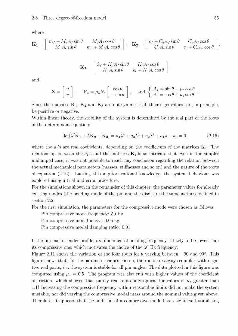
2.3. Three degree-of-freedom model 55
where
K1 =
[mf +MdAf sin θ MdAf cos θ
MdAc sin θ mc +MdAc cos θ
]
, K2 =
[cf + CdAf sin θ CdAf cos θCdAc sin θ cc + CdAc cos θ
]
,
K3 =
[kf +KdAf sin θ KdAf cos θKdAc sin θ kc +KdAc cos θ
]
,
and
X =
[uv
]
, F = µN
[cos θ− sin θ
]
, and
Af = sin θ − µ cos θAc = cos θ + µ sin θ
.
Since the matrices K1, K2 and K3 are not symmetrical, their eigenvalues can, in principle,
be positive or negative.
Within linear theory, the stability of the system is determined by the real part of the roots
of the determinant equation:
det[λ2K1 + λK2 + K3] = a4λ4 + a3λ
3 + a2λ2 + a1λ+ a0 = 0, (2.16)
where the ai’s are real coefficients, depending on the coefficients of the matrices Ki. The
relationship between the ai’s and the matrices Ki is so intricate that even in the simpler
undamped case, it was not possible to reach any conclusion regarding the relation between
the actual mechanical parameters (masses, stiffnesses and so on) and the nature of the roots
of equation (2.16). Lacking this a priori rational knowledge, the system behaviour was
explored using a trial and error procedure.
For the simulations shown in the remainder of this chapter, the parameter values for already
existing modes (the bending mode of the pin and the disc) are the same as those defined in
section 2.2.
For the first simulation, the parameters for the compressive mode were chosen as follows:
Pin compressive mode frequency: 50 Hz
Pin compressive modal mass : 0.05 kg
Pin compressive modal damping ratio: 0.01
If the pin has a slender profile, its fundamental bending frequency is likely to be lower than
its compressive one, which motivates the choice of the 50 Hz frequency.
Figure 2.11 shows the variation of the four roots for θ varying between −90 and 90o. This
figure shows that, for the parameter values chosen, the roots are always complex with nega-
tive real parts, i.e. the system is stable for all pin angles. The data plotted in this figure was
computed using µ = 0.5. The program was also run with higher values of the coefficient
of friction, which showed that purely real roots only appear for values of µ greater than
1.1! Increasing the compressive frequency within reasonable limits did not make the system
unstable, nor did varying the compressive modal mass around the nominal value given above.
Therefore, it appears that the addition of a compressive mode has a significant stabilising

56 Chapter 2. Study of a pin-on-disc lumped-parameter model
−90 −50 0 50 90−0.8
−0.6
−0.4
−0.2
Rea
l par
t
−90 −50 0 50 90−50
0
50
Pin angle θ (Deg.)
Imag
inar
y pa
rt
(a) First pair of roots
−90 −50 0 50 90
−0.2
−0.18
−0.16
Rea
l par
t
−90 −50 0 50 90
−20
0
20
Pin angle θ (Deg.)
Imag
inar
y pa
rt
(b) Second pair of roots
Figure 2.11: Three degree-of-freedom damped system. Plot showing the variation with θ ofthe two pairs of roots. µ = 0.5.
effect on the previous system (recall that the parameter values for the already existing modes
were the same as in the two-degree-of-freedom model.)
After searching for parameter values causing the system to be unstable, it appears that a
critical condition for instability to occur is that the compressive mode frequency lies between
that of the pin and disc bending mode. The system becomes more unstable as the compres-
sive frequency approaches that of the disc from the underside. The following parameter
values for the pin compressive mode give a typical example of this situation:
Pin compressive mode frequency: 25 Hz
Pin compressive modal mass : 0.03 kg
Pin compressive modal damping ratio: 0.01
Coefficient of friction: µ = 0.7.
The variation of the roots with the pin angle for this system is shown in figure 2.12. These
plots show that, with these parameter values, the system can be unstable if the pin angle
is approximately within the interval [−80 , −66]. This means that the addition of a com-
pressive mode makes it possible for the system to become unstable when the pin is trailing.
This observation is not so surprising if one recalls that, for negative angles close to −90,
the geometrical configuration of the compressive mode is actually very similar to that of
the bending mode with small positive pin angles – a configuration which was shown to be
unstable in the two-mode section. Finally, note that the imaginary parts of the roots, which
represent the frequencies of oscillation of the coupled system, are almost constant, around
25 Hz, for all pin angles.
This completes the study of the linearly stability of the three-mode system. Attention is
now turned to the behaviour of the system in a fully developed regime.

2.3. Three degree-of-freedom model 57
−90 −60 −30 0 30 60 90−1.5
−1
−0.5
0R
eal p
art
−90 −60 −30 0 30 60 90
−20
0
20
Pin angle θ (Deg.)
Imag
inar
y pa
rt
(a) First pair of roots
−90 −60 −30 0 30 60 90 −0.5
0
0.5
1
Rea
l par
t
−90 −60 −30 0 30 60 90 −50
0
50
Pin angle θ (Deg.)
Imag
inar
y pa
rt
(b) Second pair of roots
Figure 2.12: Three degree-of-freedom damped system. Plot showing the variation with θof the two pairs of roots when the compressive frequency lies between the pin and the discbending frequencies. µ = 0.7.
Nonlinear analysis
An upgraded version of the previous program computes time series simulations for this
model. The problem was first tackled numerically using the finite difference method. This
proved to work only for very small time steps and when the matrices are well conditioned.
When this is not the case, the scheme is highly unstable; high frequency oscillations can be
introduced and non-physical results can be obtained. This may indicate how difficult it is
to solve a nonlinear problem numerically. The problem is highly history dependent: each
sliding phase starts from a previous sticking point. Small errors in the determination of the
latter for instance, can lead to completely erroneous results after a surprisingly short time.
Eventually, the problem was completely solved analytically, with separate solutions for the
sticking and sliding phases. These solutions were then coded. This last implementation
proved remarkably robust.
The simulations shown next were computed using the two sets of parameter values explored in
the linear analysis above. The case when the system is always linearly stable is investigated
first (c.f. figure 2.11). The pin angle was set to θ = 5o and the coefficient of friction
µ = 0.5. In these conditions, provided the initial conditions for u and v are small enough,
the tangential velocity of the pin always remains below the disc velocity, so that sticking
never occurs. In this case, the linear theory completely solves the problem. The waveform
is simply the superposition of two sines at different frequencies. These two frequencies can
be read from figure 2.11. In general, they are not commensurable, so that the vibration is
pseudo-periodic. A time history simulation for this case is shown in figure 2.13(a). The data
plotted is the pin tangential velocity: cos θu− sin θv.
If the initial velocity or displacement given to the pin is large enough, the pin tangential

58 Chapter 2. Study of a pin-on-disc lumped-parameter model
velocity can reach the disc speed. After a first stick, the pin can settle down into a sustained
stick-slip motion if the initial energy input is sufficiently large, but in most cases, the pin
only sticks a few times, after which the vibration gradually dies out: the loss of energy by
viscous damping is greater than the amount of energy gained during sticking. Figure 2.13(b)
illustrates the latter case. The initial displacements chosen were in the vicinity of the steady
0 0.1 0.2 0.3 0.4 0.5−0.4
−0.3
−0.2
−0.1
0
0.1
0.2
0.3
0.4
Time (s)
Pin
tang
entia
l vel
ocity
(m
/s)
(a) N = 5 N, u(0) = 0.001 m, u(0) = 0,v(0) = −0.0001 m, v(0) = 0
0 0.2 0.4 0.6 0.8 1−0.8
−0.6
−0.4
−0.2
0
0.2
0.4
Time (s)
Pin
tang
entia
l vel
ocity
(m
/s)
(b) N = 5 N, u(0) = 0.01 m, u(0) = 0,v(0) = −0.0001 m, v(0) = 0
Figure 2.13: Time series simulations for the damped three degree-of-freedom system. (a)The system is always in sliding regime. (b) System exhibiting a few sticking phases.
sliding equilibrium to avoid gross initial readjustments. Unlike the two-mode model, u, v
and w all undergo oscillations, even during sticking. This makes the problem significantly
more difficult to solve mathematically. When the system damping is set to zero, similar time
series are obtained except for the decay. In this case, stick-slip oscillation can be sustained
indefinitely, following an irregular pattern.
In order to verify that the time series simulations computed for the three-degree-of-freedom
model are correct, a crosscheck is carried out. It is based on the idea that, if the pin compres-
sion stiffness is increased high enough, the simulated time series should eventually closely
resemble those obtained with the two-degree-of-freedom model. For computational reasons,
it was more convenient to increase the modal mass of the compressive mode. Figures 2.14(a-
c) show plots of the pin tangential velocity for increasing values of mc, as predicted by the
three-degree-of-freedom model. Figure 2.14(d) shows the plot obtained from simulation re-
sulting from the two-degree-of-freedom model. For these simulations, the damping was set to
zero and the coefficient of friction was again 0.5. All these time series were computed using
the following parameters: u(0) = u(0) = v(0) = v(0) = 0, N = 10 N and θ = 5. These
plots clearly show that, as mc is increased, the three-degree-of-freedom model simulations
converge towards the result obtained from the two-degree-of-freedom model. The agreement
between figure 2.14(c) and (d) is very good. A detailed observation of these last two plots

2.3. Three degree-of-freedom model 59
0 0.1 0.2 0.3 0.4 0.5
−0.4
−0.2
0
0.2
0.4
Time (s)
Pin
tang
entia
l vel
ocity
(m
/s)
(a) mc = 0.1 kg
0 0.1 0.2 0.3 0.4 0.5
−0.4
−0.2
0
0.2
0.4
Time (s)
Pin
tang
entia
l vel
ocity
(m
/s)
(b) mc = 10 kg
0 0.1 0.2 0.3 0.4 0.5
−0.4
−0.2
0
0.2
0.4
Time (s)
Pin
tang
entia
l vel
ocity
(m
/s)
(c) mc = 1000 kg
0 0.1 0.2 0.3 0.4 0.5
−0.4
−0.2
0
0.2
0.4
Time (s)
Pin
tang
entia
l vel
ocity
(m
/s)
(d) Two-degree-of-freedom model
Figure 2.14: Time series simulation for the three degree-of-freedom damped system showingthat the solution converge to the two-degree-of-freedom result as the compressive mode is madeincreasingly stiff. For computational reasons, it was more convenient to increase the mass whilekeeping the compressive natural frequency constant. Plot (d) shows the corresponding resultfrom the two-degree-of-freedom model.
shows that the times of first stick and first slip match within one time step (2E-5 s). This
strengthens one’s confidence in the results presented in this section.
To complete this study, a last case of fully developed regime will be described. The parameter
values are now chosen so that the coupled system is unstable according to the linear theory.
The second set of parameters producing the roots shown in figure 2.12 are used. Of particular
interest in relation to brake noise is to observe how a small perturbation of the steady sliding
condition might evolve. Therefore, the initial conditions were chosen such that the system
is close to static equilibrium, as produced by the preload. The following values were used:
N = 5 N, u(0) = 0.0018 m, u(0) = 0, v(0) = 0.0051 m, v(0) = 0. The pin angle θ was set

60 Chapter 2. Study of a pin-on-disc lumped-parameter model
to −70, i.e. in the range of instability. Figure 2.15 shows the time series simulation of the
pin tangential velocity. The two plots in figure 2.15 show the same data. Figure 2.15(a) is
0 0.2 0.4 0.6 0.8 1
−0.4
−0.2
0
0.2
0.4
Time (s)
Pin
tang
entia
l vel
ocity
(m
/s)
(a) Short time sample
0 1 2 3 4 5 6 7−0.8
−0.6
−0.4
−0.2
0
0.2
0.4
Time (s)P
in ta
ngen
tial v
eloc
ity (
m/s
)
(b) Long time sample
Figure 2.15: Time series simulations of the nonlinear regime of the three degree-of-freedomsystem when the underlying linear system is unstable. Plot (b) shows how the system settlesinto a permanent regime of stick-slip oscillation, after the initial transient phase shown in (a).
a zoom of figure 2.15(b) on the part showing the initial growth. Figure 2.15(b) shows how,
after a transient period (from about 0.6 s to about 4-5 s), the vibration settles into a regime
of periodic stick-slip oscillation with constant amplitude.
2.3.1 Conclusion for the three-degree-of-freedom model
In this section, the previous two-degree-of-freedom model was improved by the addition of a
compressive mode on the pin. This proved to alter significantly the behaviour of the previous
two-mode model. When the frequency of the compressive mode is above that of the disc
mode, the system is greatly stabilised as none of the previous regions of instability could
be observed. When the compressive modal frequency lies between the pin and disc bending
frequencies, the system again behaved in a completely different way from what could be
observed without the compressive mode. Instability can then arise for a narrow range of
negative angles, close to −90. The next chapter will shed a new light on these somewhat
puzzling observations. The nonlinear analysis showed that the growing vibration in a linearly
unstable system can be limited by periodic stick-slip oscillations. Periodic oscillations can
also be obtained for a lightly damped system, stable according to linear theory, but receiving
a large amount of energy from the initial conditions.

2.4. Conclusion 61
2.4 Conclusion
The models examined in this section, despite their simplicity, illustrate most of the conclu-
sions of the sprag-slip theory, namely:
• A high coefficient of friction tends to make a linear system less stable. Stick-
slip oscillation can be predicted even without any distinction between static and dynamic
coefficient of friction.
• The pin angle plays a critical role in the stability of the system. It is the geometrical
property of the system which intrinsically couples the normal and the tangential degrees of
freedom.
• The role of damping is ambiguous. In general, it has the expected effect of stabil-
ising the system but it may, for some parameter combinations, introduce instability where
the corresponding undamped system is stable.
Throughout this chapter, the distinction between linear and nonlinear analysis was empha-
sized. It was shown that the linear analysis chiefly involves solving a polynomial equation
whereas the simulation of the fully developed nonlinear regime requires accurate time histo-
ries, and a detailed modelling of the nonlinear feature (in this case, the stick-slip transition,
which is governed by the exact shape of the friction law). A slightly different model would
probably have resulted in significantly different fully developed regimes.
The modelling strategy adopted in this chapter is quite typical of brake noise studies: a
system, somewhat simpler than a brake assembly, is taken as an object of study. Its behaviour
is investigated analytically by writing equations intended to model the features assumed to
be essential. This chapter showed that, even within linear theory, the choice of dynamical
features included in the model can have dramatic consequences on the prediction. Two
plausible models yielded very different predictions. Furthermore, it was shown that assessing
the system dynamical properties accurately could be very important. In practice this can
be difficult, and this difficultly is characteristic of lumped-parameter models.
In the following two chapters, a more general type of modelling is proposed, which partly
alleviates these difficulties.

62 Chapter 2. Study of a pin-on-disc lumped-parameter model

Chapter 3
Theory of linear instability in systemswith a sliding point contact
3.1 Introduction
Within very broad limits, any system comprising a sliding frictional contact seems to be
prone to self-excited vibration and when it happens it generally exhibits a characteristic
“capriciousness”: the rig will be switched on and might immediately make a noise with
a given frequency. If it is turned off and on again an hour later, it may be silent, or
produce a noise at a different frequency... This capriciousness is often discouraging for
the experimentalist, and it is tempting to blame this feature on the numerous parameters
potentially influencing the phenomenon (temperature, humidity, normal load, geometrical
details, contacting materials...) Squeal, or whatever word may be used to describe the
phenomenon, is a “problem waiting to happen”, always on the brink of occurring, and often
with several different types of squeal available to be “chosen” by the system.
This apparently generic behaviour cannot be investigated in a very illuminating way by
analysing specific systems because the details obscure any possible generality. In this chapter,
a unified analysis of a rather more general class of systems is presented. Some conclusions can
be drawn from this analysis, about which characteristics of a system may make it prone to
squeal, and about the origin of capriciousness. For definiteness this account will be presented
in terms of noise in disc braking systems, although the theory to be presented applies equally
well to self-excited vibration in a variety of other systems containing a sliding point contact.
The systems to be studied, although general in some respects, are still very particular in
other respects. The aim is to study a class of systems which are as simple as possible, while
retaining an essential aspect of generality. Two important restrictions apply:
(1) this is a linearised stability analysis,
(2) contact only occurs at a single point.
Only squeal events which can be initiated via linear instability of the state of steady sliding
are considered. There may well be some types of squeal which rely on intrinsically nonlinear
phenomena such as parametric resonance, or the possibility, seen in the previous chapter,
that a periodic or non-periodic vibration could be sustained at finite amplitude without the
63

64 Chapter 3. Theory of linear instability in systems with a sliding point contact
necessity of instability when the underlying system is linearised. Equally, squeal may be ini-
tiated by a linear instability, but it may change its character significantly as it grows to large
amplitude: harmonics may be generated, and the frequency may shift, either continuously
or by jumping to a subharmonic, for example following a period-doubling bifurcation. These
are all issues worthy of investigation. However, a clear understanding of the linear problem
is surely a prerequisite for any further study.
3.2 Governing equations
The system to be studied is shown diagrammatically in figure 3.1. One linear system, thePSfrag replacements
N
N
F
F
‘Disc’ ‘Brake’
Dis
cR
otat
ion
① ②
v1
u1
u2
v2
Figure 3.1: Diagram showing two linear systems in sliding contact at a single point. Dis-placements ui and vi apply at the contact point but are shown shifted apart for clarity.
‘disc’, is being driven in uniform motion. Another linear system, the ‘brake’, is stationary
apart from vibration, and makes contact with the first system through a single point. All
motion is assumed to take place in the plane of the diagram, which is also the plane of
the imposed frictional sliding. At the contact point, there is a pair of equal and opposite
normal reactions N acting on the two systems, and similarly a pair of equal and opposite
friction forces F . These forces are both composed of a steady component plus a fluctuating
component which will be assumed to be small:
N = N0 +N ′, F = F0 + F ′. (3.1)
Denote the normal and tangential displacements of the disc by u1 and v1 respectively, and
the normal and tangential displacements of the brake by u2 and v2 respectively. The tan-
gential displacement of the disc needed here is that due to the vibration alone, disregarding
the contribution from steady rotation. All fluctuating quantities will be considered in the
frequency domain, as Fourier Transforms of the associated time-varying quantities. The
Fourier frequency variable is denoted ω. The goal of this analysis is to study the initiation
of self-excited vibration from a state of steady sliding and all motion will be assumed to be
sufficiently small for linear theory to be used.

3.2. Governing equations 65
The displacements of each system are related to the normal and tangential forces via the
matrices of transfer functions defined by
[u1
v1
]
=
[G11(ω) G12(ω)G21(ω) G22(ω)
] [N ′
F ′
]
,
[u2
v2
]
=
[H11(ω) H12(ω)H21(ω) H22(ω)
] [N ′
F ′
]
(3.2)
The matrices are both symmetric from the standard principle of reciprocity (e.g. Skudrzyk
(1968)). In practice, violation of symmetry could arise from the rotation of the disc, but this
rotation will be assumed to be sufficiently slow for the effect to be neglected. To obtain a
closed system of equations, two further relations are required. First, it is assumed that the
brake and disc remain in contact, but some input to the linear system is allowed via surface
roughness of the disc. This means that the two normal displacements are equal and opposite
except for the effect of roughness, defined by a function (again in the frequency domain) r
which is assumed known. Then
u2 = r − u1. (3.3)
Finally, a frictional constitutive law is needed. In this chapter, the simplest possible as-
sumption is made whereby the friction force F is proportional to the normal force N with a
constant coefficient of friction µ:
F = µN. (3.4)
In the next chapter, the effect of a more complicated friction law will be investigated. The
sign convention in figure 3.1 has been chosen so that a positive value of µ is expected.
The set of equations including the simple friction law (3.4) can be straightforwardly rear-
ranged to give the solution:
N ′ =r
G11 + µG12 +H11 + µH12
(3.5)
and
u1 = (G11 + µG12)N′
v1 = (G12 + µG22)N′
u2 = (H11 + µH12)N′
v2 = (H12 + µH22)N′
(3.6)
Since all the individual transfer functions Gij, Hij are of stable systems, all poles are in the
upper half of the complex Fourier plane.

66 Chapter 3. Theory of linear instability in systems with a sliding point contact
It follows immediately that
This system can be unstable if and only if the function
D(ω) = G11 + µG12 +H11 + µH12 (3.7)
has at least one zero in the lower Fourier half-plane.
So far, ω has been used as a complex variable, as opposed to the Laplace variable s, more
familiar in control. This choice is somewhat arbitrary. It matters little as long as the corre-
spondence is clear. The domain of stability for the Laplace variable s is the left hand side
complex plane, so that t 7−→ est remains bounded. For t 7−→ eiωt to remain bounded, the
Fourier variable ω must be in the upper half-complex plane. The upper half complex plane
is therefore the domain of stability. The variable ω will be used throughout this chapter, its
relation to s is simply s = iω.
The framed statement above is the key theoretical result of this thesis. Much of what follows
will be based on exploring this equation from different points of view. The rationale behind
the rest of this chapter is as follows. First, this condition for instability will be analysed
in general terms, as some useful information can indeed be gained from a purely formal
inspection. Then, the criterion will be tested by simulations of increasing complexity.
3.3 Some general observations
This section consists of a series of subsections. Each subsection throws some light from a
different angle on the general criterion derived above. They may first appear unrelated to
each other, but the order of the sequence is essential, as most of the properties derived in
one subsection are used in the next. First, we start with a useful simplification.
3.3.1 Cross-term of the disc
If the first subsystem is indeed a model of a brake disc, or a brake drum, then to a good
approximation there is a plane of symmetry through the contact point and the centre of the
disc/drum. It follows immediately that
G12 = 0 , (3.8)
since tangential forces and displacements are anti-symmetric with respect to this plane, while
normal forces and displacements are symmetric so that they cannot interact. If this is indeed
the case, then the function D(ω) reduces to:
D(ω) = G11 +H11 + µH12 . (3.9)
Throughout this chapter and the next, G12 will be assumed to be zero. Equation (3.9) shows
that, within the linear theory, the coefficient of friction only influences the stability via the

3.3. Some general observations 67
dynamic cross-coupling of the pin. If the pin subsystem is also symmetrical so that H12 = 0,
then the coefficient of friction no longer enters the formulation. D is then further reduced to
D(ω) = G11+H11, which simply expresses the passive normal coupling of the two subsystem.
One expects such a system to be always stable. This is confirmed, if the transfer functions
are expressed in terms of modal parameters.
3.3.2 Expression of D(ω) in terms of modal parameters
The transfer function G11 is a driving-point receptance, which can be expressed in terms of
the mode shapes φn, their natural frequencies ωdn and their modal damping factors δn using
the standard formula
G11(ω) =∑
n
φ2n(x)
ωd2n + 2iωωd
nδdn − ω2
, (3.10)
where φn(x) denotes the value of the (mass-normalised) mode shape at the position of the
contact point, in the normal direction. Proportional damping has been assumed here, for
simplicity. The effect of non-proportional damping will be discussed in the next chapter.
In a very similar way, the transfer functions H11 and H12 can be expressed in terms of the
brake mode shapes ψn, their natural frequencies ωbn and their damping factors δb
n
H11(ω) =∑
n
ψ2n(x)
ωb2n + 2iωωb
nδbn − ω2
, H12(ω) =∑
n
ψn(x)ψn(y)
ωb2n + 2iωωb
nδbn − ω2
, (3.11)
where ψn(x) denotes the value of the (mass-normalised) mode shape at the position of the
contact point, in the normal direction, and ψn(y) denotes the corresponding mode shape in
the tangential direction. Thus
D(ω) =∑
n
φ2n(x)
ωd2n + 2iωωd
nδdn − ω2
+∑
n
ψn(x)[ψn(x) + µψn(y)]
ωb2n + 2iωωb
nδbn − ω2
. (3.12)
The function D(ω) has the functional form of a transfer function, although it is not the trans-
fer function of any obvious physical system. However, the zeros of D may, in some sense, be
thought of as the complex eigenvalues of the coupled system. The fact that D has the form
of a transfer function means that its characteristics can be deduced from standard arguments
about the distribution of peaks and anti-resonances (Skudrzyk (1968)). The frequencies ωn
must be appropriately interleaved to give the full set of peaks in this function. Between
an adjacent pair of peaks, there will either be a shallow dip or a sharp anti-resonance. If
the coefficients of the resonant terms in the expansion (3.12) have the same sign, an anti-
resonance generally occurs, while if they have opposite signs, a shallow dip occurs. This
distinction is important for the present investigation: to predict the threshold of instability,
we are interested in the zeros of D and particularly in zeros which are very close to the real
ω axis, either just above (and thus stable) or just below (and thus unstable). Such zeros,
which are near the stability threshold, will occur close to the anti-resonance frequencies of

68 Chapter 3. Theory of linear instability in systems with a sliding point contact
D. This idea will be pursued in the simulation section. However, this already suggests that
the signs of the modal coefficients play an important part in the stability of the system.
From equation (3.12), it appears that many of the amplitude coefficients will be positive,
because they come from driving point transfer functions. Only those coming from the brake
can be negative depending on the magnitude of the coefficient of friction, and the sign and
magnitude of ψn(x) and ψn(y).
3.3.3 The algebraic point of view
To investigate the formal properties of D(ω), it is useful to consider the resonant terms
in expansion (3.12) as belonging to a single pool of “modal blocks”, regardless of which
subsystem they come from. It is also convenient to write the combinations of mode shape
coefficients appearing at the numerators in equation (3.12) as single coefficients ai. The
function D(ω) can then be written:
D(ω) =a1
ω21 + 2iω1δ1ω − ω2
+a2
ω22 + 2iω2δ2ω − ω2
+a3
ω23 + 2iω3δ3ω − ω2
+a4
ω24 + 2iω4δ4ω − ω2
...(3.13)
This form will often be used as the basis for simulations, because it reduces slightly the large
number of parameters involved. For convenience, the coefficients ai in equation (3.13) will be
referred to as “modal amplitudes”, although they probably do not represent the amplitude
of any physical variable of the system.
In equation (3.13), D(ω) appears as the sum of rational fractions of degree −2. Putting these
fractions to the same denominator, D can be written as a single ratio of two polynomials,
say P and Q, so that D(ω) = P (ω)/Q(ω). The roots of Q(ω), which are the poles of D(ω),
are the roots of the quadratic denominators appearing in expansion (3.12). These poles have
a simple approximate expression: ωi(1 + iδi) and ωi(−1 + iδi). The zeros of D(ω) are simply
the roots of P (ω). P has a number of remarkable properties:
(1) If D consists of Ntot resonant terms, the degree of P will be 2(Ntot − 1). Therefore P
will have 2(Ntot − 1) roots and D has as many zeros.
(2) P (iω) has real coefficients. Therefore the roots of P (iω) are either real or form a pair
of complex conjugates. Consequently, the zeros of D(ω) are either purely imaginary or
appear as “−i” times a complex conjugate pair. In geometrical terms, this means that
the pattern of zeros is symmetrical with respect to the imaginary axis in the complex
ω-plane. For the same reason, the pattern of poles of D has the same property.
(3) The coefficients of P are made of linear combinations of homogeneous products of ωi
and δi. They always depend linearly on the ai. Each coefficient is invariant under
circular permutation of the indices.

3.3. Some general observations 69
(4) The leading coefficient of P (ω) is always the sum of the ai. When this sum equals
zero, the degree of P drops by one and so does the number of roots. Therefore, one
can expect the condition∑ai = 0 to appear as a remarkable event.
(5) The odd-power coefficients of P always consist of linear combinations of damping
factors. This has two important consequences. First, if the system is undamped, P
only has even power of ω, so that the pattern of roots will be symmetrical with respect
to both the real and imaginary (from (2)) axes. Second, if the damping in non-zero
but light, the coefficients of odd powers in P will nevertheless have a significantly lower
order of magnitude than those of even power, so that, in that case too, the pattern of
roots can be expected to be almost symmetrical with respect to the real axis, in the
ω-complex plane.
(6) The root-coefficient relationships ensure that if the coefficients of Ps(s) = P (−iω) have
different signs, the system is unstable (see e.g. Dorf (1980)). It is easier to see that
if the roots of P (−iω) are all in the left-hand side of the complex plane, then all the
coefficients of P (−iω) have the same sign. However, if the coefficients of P all have
the same sign, no conclusion regarding the stability can be drawn from this argument:
the system can be stable or unstable.
These properties are simply listed here. They are either standard results on polynomials,
are straightforward, or they become clear once the expression for P is written down for a
function D containing two terms. It is noteworthy that P possesses remarkable symmetry
properties (e.g. (3)), from which some information might be drawn, regarding the location
of the roots in the complex plane. However, it was impossible to develop this line of inquiry
further within the scope of the thesis. Property (6) is clearly of interest for this study, as
it links the modal properties of the two subsystems, through the coefficients of P , to the
stability of the coupled system. The next subsection refines this property.
3.3.4 The complex analysis point of view
In principle, the number of unstable zeros of D(ω) could be obtained using the Nyquist
criterion, familiar from control theory (see e.g. Dorf (1980)). This would amount to defining
a contour consisting of a large portion of the real axis, closed by a semi-circle in the lower
half complex plane (unstable region). A typical situation is represented diagrammatically
in figure 3.2, where the crosses represent the poles and the circles, the zeros of D(ω). This
plot shows two unstable zeros in the lower half plane, encircled by the contour labelled Γ.
Nyquist’s criterion1 states that the number of zeros inside the semi-circular contour is equal
to the number of times the curve obtained by plotting D(ω) as ω moves along Γ, encircles
the origin.
1The statement of the criterion given here has been tailored to our particular situation: the standardversion works within the Laplace domain and also gives a count of the unstable poles.

70 Chapter 3. Theory of linear instability in systems with a sliding point contact
PSfrag replacements
Γ
R
R
−R
Re
Im
Figure 3.2: Plot showing diagrammatically a typical contour Γ, in the Fourier complexplane. The crosses represent the poles of D, while the circles represent the zeros. The polesare always in the upper half plane. The zeros can be in the upper (stable) or lower (unstable)half complex plane. The patterns of zeros and poles are both symmetrical with respect to theimaginary axis. The two unstable zeros are encircled by the semi-circular contour of radius R,labelled Γ.
In practice, counting these encirclements when D contains many modes can be difficult,
because the image curve D(Γ) usually follows a very intricate path. But the criterion can
be used to prove an interesting result, refining the property (6) given in the previous section.
The claim is that the function D(ω) cannot have any zero in the lower half complex plane
if all the “modal amplitude” coefficients ai are positive. A sketch of the proof is given in
Appendix A. It is based on the fact that if the ai are all positive, then, as ω moves along
the path Γ, the image path D(Γ) cannot take real negative values. Therefore, it cannot
encircle the origin.
Property (6) gives a condition on the coefficients of P for instability to occur. However, most
of the coefficients of P are a complicated mixture of ai, ωi and δi. The property derived
from Nyquist’s criterion gives a condition involving the ai themselves. The ai are more
directly related to the mechanical properties of the two subsystems. It was mentioned in
section (3.3.2), that ai can only be negative when it comes from a brake mode. Its expression
in terms of mode shapes is then:
ai = ψ2i (x) + µψi(x)ψi(y). (3.14)
The first term cannot be negative, therefore, the coupled system can only be unstable if the
cross-term ψi(x)ψi(y) is negative. If this product is negative, large values of the coefficient of
friction µ can contribute to make the whole modal coefficient ai negative, thus making the
system more prone to instability. This feature was already mentioned in the literature review
as a broadly-agreed conclusion of the sprag-slip theory. Conversely, rotating the disc in the
opposite direction amounts to using a negative coefficient of friction in D(ω). Therefore, the
modes of the brakes such that ψi(x)ψi(y) > 0 could then become destabilising if the disc is
rotated in the opposite direction. A negative value for ψi(x)ψi(y) can be given an interesting
physical interpretation: it points towards the importance of those modes of the brakes whose

3.3. Some general observations 71
tangential and normal motion are out of phase. With the sign conventions of figure 3.1, the
potentially destabilising modes are those whose tangential motion opposes the rotation of
the disc as the brake pushes toward the disc in the normal direction. This is reminiscent
of the digging-in angles found to cause instability in the pin-on-disc model investigated in
Chapter 2.
3.3.5 Application to the pin-on-disc system
The lumped-parameter models studied in Chapter 2 are now revisited in the light of the
theory presented in this chapter. First, it seems useful to verify that the theory introduced
in this chapter gives the same linear stability prediction as that found for the particular
linear systems studied in Chapter 2. To this end, the equations governing the stability of
the two-degree-of-freedom system presented in Chapter 2 were cast into the new transfer
function formulation. This is done in Appendix B, where it can be seen that both the direct
method used in Chapter 2 and the present theory lead to the same stability equation.
In the two-mode model, the pin/brake had only one mode. From Appendix B, it appears
that the quantity corresponding to
ψ2i (x) + µψi(x)ψi(y) is
sin2 θ − µ sin θ cos θ
mf
In this simple case, there is therefore a direct correspondence between the new formulation
and the pin-on-disc system. This suggests that however complicated a single point contact
system may be, for each mode of the brake there is an underlying simple pin-on-disc system
with an equivalent pin angle. This equivalent pin angle could be obtained from the relation:
tan θi =ψi(x)
ψi(y)
For any instability to arise, one of the modes of the brake must be such that its equivalent
pin angle lies within the range [0 θ], where θ is such that tan θ = µ.
This sheds a new light on the behaviour of the three-mode system described in Chapter 2.
There, it was found that instability did not arise from the bending mode, as in the two-mode
model, but it originated from the compressive mode. Since the mass-spring system for this
mode is at 90 to the bending mode, its sector of possible instability will be rotated by 90
as well. Therefore, this system has two sectors of instability. With the parameter values
tested in Chapter 2, instability could only be obtained within the second sector. This is
summarised in figure 3.3
In conclusion, the application of the theory to the two systems previously studied confirms
its validity. It also shows that the formalism introduced in this chapter indeed generalises the
approach followed in Chapter 2, since it includes in a single formula the stability equation of
a whole class of systems. Reciprocally, the simplest pin-on-disc system studied in Chapter 2
can be used as a paradigmatic example to understand the behaviour of each individual mode

72 Chapter 3. Theory of linear instability in systems with a sliding point contact
PSfrag replacements
θ
Disc
(a) Two-mode system
PSfrag replacements
θ
θ
Disc
(b) Three-mode system
Figure 3.3: Drawings showing the pin angle sectors where the system is potentially unstable.(a) for the two-mode system. (b) for the three-mode system. θ is such that tan θ = µ.
of the brake.
3.3.6 Summary of the general properties
In this section, new assumptions have been introduced and consequences have been derived
from them. Throughout this chapter, these assumptions will be supposed to be valid. There-
fore, it seems useful to recapitulate the most important hypotheses and conclusions.
• If the disc is symmetrical, then the cross transfer functions of disc admittance matrix G
will be zero. This simplifies the expression forD(ω). It also follows from this hypothesis
that the coefficient of friction can only affect the system via the cross transfer function
of the brake subsystem.
• If proportional damping is assumed, then D(ω) can be expressed as a standard transfer
function involving the real modes of the two subsystems. Written in this form, the
zeros of D(ω) are the roots of a polynomial P , such that P (iω) has real coefficients.
This results in symmetry properties for the pattern of roots. Proportional damping
(i.e. real mode shapes) for the two subsystems is also essential to the property that
no instability can occur if the “composite” modal amplitudes ai are all positive.
This completes the general comments that could be made on the theory introduced in this
chapter. In the next section, a number of approximate systems will be investigated using
this formalism. These analyses will now be local: a system will approximated by a number
of neighbouring modes. Most of the general comments made in this section will re-emerge,
often as elementary mathematical properties of the particular system under investigation.

3.4. Approximate analysis of generic systems 73
3.4 Approximate analysis of generic systems
The previous sections point towards the study of the zeros of transfer functions. It is more
customary to study poles of transfer functions. Coming from a different perspective, Lyon
and coworkers (Lyon (1983, 1984), Tohyama and Lyon (1989)) have made some useful ob-
servations on the location of transfer function zeros and their relation to the phase of the
frequency response. The results presented in this section can be thought of as an extension
of Lyon’s work. Section (3.3) produced some general observations on the behaviour of D(ω).
In this section, the approach taken is the reverse of the usual one, exemplified in Chapter 2,
whereby a given physical system is modelled by writing down equations, using mechanical
parameters. Here, a particular system will be modelled within a particular frequency range.
The results are based on the usual assumption that, however complicated the function D(ω)
for a particular system, one can usually expect to obtain a reasonable approximation in
the vicinity of a given frequency by considering only the nearby resonances. Therefore, this
approach is only expected to give meaningful results where this assumption is valid, that is,
in the vicinity of a given particular frequency, for instance that of a squeal event. In this
section, various approximations of increasing complexity will be investigated. The simplest
useful approximation which can lead to a prediction about zeros of D(ω) is to consider just
two terms, and neglect all others. This case is so simple that it can be dealt with in some
detail. The influence of additional terms from distant resonances will then be considered.
3.4.1 Two-mode approximation
The two-mode approximation can be useful if the system squeals at a frequency in the
vicinity of which there are two relatively isolated modes of the uncoupled subsystems. In
this context, the function D will have the form:
D(ω) ≈ a1
ω21 + 2iω1δ1ω − ω2
+a2
ω22 + 2iω2δ2ω − ω2
, (3.15)
Suppose, for example, that the first term comes from mode n of the disc, while the second
comes from mode m of the brake. Then using the notation defined in the previous section,
a1 = φ2n(x) , ω1 = ωd
n , δ1 = δdn ,
and a2 = ψ2m(x) + µψm(x)ψm(y) , ω2 = ωb
m , δ2 = δbm .
(3.16)
Positive-frequency pole approximation
As well as neglecting all but two terms in equation (3.12), further simplification can be
obtained by factorising the denominator expressions, which are quadratic in ω, expressing
each term as a sum of two partial fractions and retaining only the one with a resonance at a
positive value of Re(ω). The second term, with a negative value of Re(ω), is typically more
distant than the other neglected resonances of the system. This leads to the approximation:
D(ω) ≈ c1ω − ω1
+c2
ω − ω2
, (3.17)

74 Chapter 3. Theory of linear instability in systems with a sliding point contact
where
ωk ≈ ωk(1 + iδk) and ck = − ak
2ωk
(k = 1 or 2) (3.18)
are respectively the positive-frequency poles of the modes retained, and c1 and c2 their
corresponding residues. By convention, whenever the term “residue” is used in an unspecified
way in the remainder of this chapter, it will always be understood as the residue associated
with positive-frequency pole.
The one complex zero ω = ωz resulting from this approximation is simply
ωz ≈c1ω2 + c2ω1
c1 + c2. (3.19)
From equation (3.19), it is clear that, whatever the values of c1 and c2, ωz always lies on
the straight line passing through ω1 and ω2 in the complex plane. The slope of this line
depends on the ratio of damping factors of the two modes (this slope depends on their
natural frequencies as well, but these are assumed to be close). If the poles have similar
imaginary parts, the pole line will be almost parallel to the real axis and will only cross it
far away from the the poles. In that case, the present approximation is not expected to hold
since the influence of other poles may no longer be negligible. On the other hand, if the
two damping factors are very different, the line will have a large slope and will cross the
real axis to produce potential instability not too far from the poles. This suggests that if
two neighboring modes have very different damping factors, then instability is more likely
to arise in the vicinity of these two modes.
If c1 and c2 both have the same sign, then ωz is simply a weighted average of the two complex
poles and therefore lies in between them. Since the two poles are stable, they both lie in the
upper half complex plane and so do all the points on the segment joining them. Thus, this
combination cannot lead to an unstable zero.
More interesting is the case when c1 and c2 have opposite signs. Note that given the sign
reversal between the residues ci and the modal amplitudes ai (see equation (3.18)), the
residues of the disc can only be negative, while those of the brake can be positive or negative,
(provided the mode shapes are real, as implied by the assumption of proportional damping).
Two cases may be distinguished. Suppose first that c1 < 0, c2 > 0 and c1 + c2 < 0. Then
ωz = ω2 + α(ω2 − ω1) with α = − c2c1 + c2
(3.20)
The zero occurs on the opposite side of ω2 from ω1, and if α is reasonably small it will be
close to ω2. It may, of course, be influenced by the next resonance on that side of ω2, but it is
supposed that ω1 and ω2 are close together compared to the interval to the next resonance,
so that this possibility can be temporarily ignored. This zero can be unstable if
−αIm(ω1) + (1 + α)Im(ω2) < 0 (3.21)
or, using equations (3.16) and (3.18)
δbm <
(α
1 + α
)(ωd
n
ωbm
)
δdn. (3.22)

3.4. Approximate analysis of generic systems 75
Instability can occur if the damping of the brake mode is sufficiently small. Figure 3.4
shows a plot of the function D(ω) for a typical example of the behaviour just discussed, with
parameter values producing an unstable zero.
0 0.5 1 1.5 2 2.5 3−50
−40
−30
−20
−10
0
10
20
30
Frequency
Log
Am
plitu
de (
dB)
(a)
0 0.5 1 1.5 2 2.5 3−25
−20
−15
−10
−5
0
5
10
15
Frequency
Rea
l and
imag
inar
y pa
rts
(b)
Figure 3.4: Plot of D showing a zero (antiresonance) beyond the two fixed poles at frequencies1 and 1.5 rad/s. The damping factors were 0.02 and 0.01 respectively and the residues −1 and0.5 in the same order. (a) Magnitude plot of D (in dB). (b) Plot of the real (solid line) andimaginary (dashed line) parts of D (linear scale).
The second case occurs when c1 < 0, c2 > 0, c1 + c2 > 0 and yields very similar results so
only the main points are given here: this time the zero occurs on the opposite side of ω1
from ω2 and it can be unstable if
δbm >
(1 + β
β
)(ωd
n
ωbm
)
δdn, with β = − c1
c1 + c2> 0 . (3.23)
In this case, instability can occur if the damping of the brake mode is sufficiently large.
This two-pole analysis suggests that:
(1) a prerequisite for the occurrence of instability is the presence of consecutive, out-
of-phase modes.
(2) the stability of the system is significantly influenced by the damping. As far as
stability is concerned, the relative magnitude of the damping factors seems to matter more
than their absolute values.
Influence of the negative-frequency poles
To verify how much these conclusions are specifically linked to the “positive-pole” approx-
imation, the stability of the system is now studied with the negative poles added back in.

76 Chapter 3. Theory of linear instability in systems with a sliding point contact
To compare the two approximations, it is more convenient to use the modal amplitudes ai,
rather than residues ci. The function D for this system was expressed in equation (3.15).
Its zeros are the roots of the following quadratic equation:
(a1 + a2)(iω)2 + 2(a1ω2δ2 + a2ω1δ1)(iω) + a1ω22 + a2ω
21 = 0 (3.24)
In order to analyse the interaction of the two modes in a somewhat systematic way, one
mode, say mode 1 (the disc mode), has its characteristics kept fixed, while mode 2 (the
brake mode) will be varied in frequency and amplitude. This will also set the scene for the
subsequent approximations, where this procedure will be used extensively. To study the
stability, one could express the roots of equation (3.24), but this does not lend itself to an
easy treatment. Written as a polynomial in s = iω, it is possible to use the Routh-Hurwitz
criterion to determine the stability of the roots of equation (3.24). For a quadratic, the set
of conditions for the system to be stable is simply that all the coefficients should have the
same sign, either positive or negative:
(1) a1 + a2 > 0(2) a1ω2δ2 + a2ω1δ1 > 0(3) a1ω
22 + a2ω
21 > 0
or
(1) a1 + a2 < 0(2) a1ω2δ2 + a2ω1δ1 < 0(3) a1ω
22 + a2ω
21 < 0
. (3.25)
From these two sets of inequalities, it is clear that the system is always stable if the two modal
amplitudes have the same sign. This conclusion was already reached from the positive-pole
approximation. From the definitions of a1 and a2 given in equation (3.16), a1 is always
positive, and only a2 can be positive or negative. Since it is the only interesting case, a2 will
be assumed to be negative.
If a2 and ω2 are varied, these two sets of conditions can be represented as areas in the
(ω2, a2)-plane. These areas of stability are delimited by three curves whose equations are
given by setting each condition in equation (3.16) to zero. The first condition is simply a
horizontal line at −a2 = a1, cutting the plane into two parts. Condition (2) also defines two
regions, delimited by the straight line −a2 = a1δ2
δ1ω1
ω2, while the third condition defines two
areas delimited by a parabola of equation −a2 = a1ω22/ω
21. The domain of stability is the
intersection of all these areas. Note that only condition (2) involves the damping factors.
This means that conditions (1) and (3) remain unchanged whatever the system damping.
Figure 3.5 consists of three plots showing the stability domain as a shaded area for three
different values of the damping factor ratio. For these plots, Mode 1 has both its frequency
and modal amplitude set to 1. The damping factor is 0.01. Mode 2 is varied in natural
frequency from 0 to 2, and in modal amplitude from -5 to 0. These plots are particularly
useful to understand how the damping affects the stability regions. As already noted, the
damping factors are only involved in condition (2), through their ratio. If they are identical,
as in figure 3.5(c), the three curves meet at a single point (ω1, a1), so that the line resulting
from condition (2) does not modify the regions of stability defined by conditions (1) and (3)
alone. Therefore the stability domain showed in figure 3.5(c) is also the stability domain
of the undamped system. This feature will recur many times in the subsequent sections:

3.4. Approximate analysis of generic systems 77
ω 2
− a
2
0.5 1 1.5 20
1
2
3
4
5
(a) δ2/δ1 = 3/2
ω 2
− a
2
0.5 1 1.5 20
1
2
3
4
5
(b) δ2/δ1 = 2/3
ω 2
− a
2
0.5 1 1.5 20
1
2
3
4
5
(c) δ2/δ1 = 1
Figure 3.5: Plots showing the domain of stability of a two-mode system for different valuesof the damping factors. The properties of Mode 1 are fixed at frequency 1, modal amplitude1 and damping factor 0.01. The natural frequency of mode 2 is varied from 0 to 2, while itsmodal amplitude is varied from −5 to 0. The three plots correspond to three damping factors:(a) δ2 = 0.015, (b) δ2 = 0.0066, (c) δ2 = 0.01. The shaded areas are the zones where thesystem is stable. The horizontal line is −a2 = a1 = 1, the dashed line is −a2 = a1
δ2δ1ω1
ω2,
while the dotted line is −a2 = a1ω22/ω
21.
if all the modes have the same damping factor, then the stability region is the same as in
the undamped case. When the damping factors are different, the line defined by condition
(2) encroaches either on the upper “undamped” stability region if δ2/δ1 > 1 (figure 3.5(a)),
or on the lower “undamped” region, if δ2/δ1 < 1 (figure 3.5(b)). The more different the
damping factors, the more the stability region is reduced. This behaviour was also observed
in the two-pole analysis. In contrast to the latter, the present analysis predicts the existence
of instability, even if the system is undamped (the single zero predicted by the two-pole
analysis is always marginally stable if the system is undamped.) Subsequent analyses will
throw some light on this particular point.
It may be objected at this point that the range of variation of the second mode frequency
may be too large for a local analysis: if a normalised frequency equal to 1 represents 1
kHz, then varying the second frequency between 0 and 2 means varying it between 0 and
2 kHz! A real system would probably have many other modes within this range, which
makes the assumption that the two frequencies are relatively isolated very implausible. This
objection is probably fair. The reason for choosing such a wide range is that it gives a good
understanding of how the plots showing thresholds of stability (figure 3.5) are constructed.
These plots will recur many times throughout this work. Most of the features described
here will still be present. But the complexity of the algebra will prevent the clear analytical
understanding reached with this simple case. This is particularly true of the influence of
damping.
To conclude this section, the two approximations discussed so far are compared. Figure 3.6
shows the stability threshold lines for the two approximations. The solid line is obtained

78 Chapter 3. Theory of linear instability in systems with a sliding point contact
0.8 0.9 1 1.1 1.20
0.5
1
1.5
2
2.5
ω 2
− a
2
Figure 3.6: Plot showing the stability thresholds of a two-mode system. One mode is keptfixed with frequency 1, amplitude 1 and damping factor 0.01, while the other mode is varied infrequency ω2, and amplitude a2, within the ranges of the plot. The dashed line is the stabilitythreshold when only the positive-frequency poles are considered; the solid line, when bothnegative and positive frequency poles are included. The system is unstable within each set ofline, i.e. it is stable above the top line and below the bottom line for each set.
when both positive and negative-frequency poles are included; the dashed line, when only the
positive frequency poles are taken into account. The frequency range of the varying mode has
been limited to [0.8 1.2], that is ±0.2 around the fixed mode. The plot only shows the lower
range of the varying amplitude, because there is no instability above 3 within the frequency
range considered. This plot can be thought of as a zoom on figure 3.5(a). Comparing the two
sets of lines, it appears that the agreement is broadly right. The two approximations agree
perfectly when ω2 = ω1. Discrepancies become larger as ω2 moves away from this value, as
one might expect from a local approximation. As far as “mode locking” is concerned, this
plot, and even more figure 3.5, suggest that the condition ω1 = ω2 is better seen as the limit
between two instability regions than an indication that the system is particularly unstable.
This was already observed in Chapter 2, in relation to the two-mode model. Regarding the
influence of the modal amplitude, it seems that instability is more likely to arise when the
two amplitudes are close in magnitude. However, for both types of approximations studied
so far, it is essential that these modal amplitudes have opposite signs for instability to arise.
These conclusions are provisional. In chapter 2, the two-degree-of-freedom system was shown
to exhibit a somewhat specific behaviour. The next section will present the study of a more
complex system, which will begin to indicate how much of the previous findings still hold
true.
3.4.2 Two poles plus a constant residual
The conclusions of the two-mode analysis are likely to be affected by the presence of other
poles. With more than two poles, analytical investigation is difficult because the algebra
becomes rapidly unwieldy, and with six or more poles it is in principle impossible in most

3.4. Approximate analysis of generic systems 79
cases, because it requires the roots of a polynomial of degree 5 or higher. However some
further progress is possible by supposing that around a frequency of interest, the function
D can be appropriately approximated by keeping the two nearest poles and assuming that
the contribution from more remote poles can be equated to a constant residual. Further
analytical progress can be achieved by ignoring the contribution from the negative-frequency
poles. Therefore, only the positive-frequency poles are included in the analysis presented in
this section.
With the notation introduced in the previous sections, the approximate expression for D
becomes:
D(ω) ≈ c1ω − ω1
+c2
ω − ω2
+R , (3.26)
where R is the contribution from farther poles. Denote by ω3 = ω3(1 + iδ3) one of the
remote poles contributing to R. The exact contribution of this pole to D would be a term
proportional to 1/(ω−ω3). As ω moves further away from ω3, the imaginary part of 1/(ω−ω3)
decays like 1/(ω − ω3)2, whereas its real part decays like 1/(ω − ω3), so that in the vicinity
of ω1 or ω2, the real part of 1/(ω − ω3) will dominate its imaginary part. Therefore, R will
be assumed to be real.
If D given by equation (3.26) is rearranged as a single rational fraction, its numerator is a
quadratic in ω, whose roots are:
ωz± = ω − c1 + c22R
±
√(c1 + c2
2R
)2
+ ∆2+c1 − c2R
∆, (3.27)
where
ω =ω1 + ω2
2and ∆ =
ω2 − ω1
2.
Equation (3.27) shows that ωz± can only have a negative imaginary part when the square
root possesses a negative imaginary part large enough to overcome that of ω. In order to
carry this analysis further, the system will be assumed to be undamped. For then, all the
quantities become real and it is possible to study the sign of the expression under the square
root. The influence of damping will be discussed at the end of this section. In practice,
however, the damping is usually small, so the conclusions reached for the undamped case
can be expected to remain broadly true.
The undamped case
With no damping, equation (3.27) can be conveniently rewritten
ωz± = ω − c1 + c22R
±
√(
∆ +c1 − c2
2R
)2
+c1c2R2
, (3.28)
where ω and ∆ are the (real) values of ω and ∆ when the damping is set to zero. One of
these zeros has a negative imaginary part if and only if the expression under the square root

80 Chapter 3. Theory of linear instability in systems with a sliding point contact
is negative. It is immediately clear that this can only occur if c1c2 < 0, i.e. if the residues
have opposite signs. Assume first that c1 < 0 and c2 > 0. Then
(
∆ +c1 − c2
2R
)2
+c1c2R2
= ∆2
(
1 − (√−c1 −
√c2)
2
2R∆
)(
1 − (√−c1 +
√c2)
2
2R∆
)
.
If R∆ < 0, both brackets are positive, so that the zeros cannot be complex. If R∆ > 0, the
product of the two brackets is negative whenever R∆ satisfies:
(√−c1 −
√c2)
2
2≤ R∆ ≤ (
√−c1 +√c2)
2
2. (3.29)
Similarly, when c1 > 0 and c2 < 0, instability can only arise if R∆ < 0 and satisfies:
−(√c1 +
√−c2)2
2≤ R∆ ≤ −(
√c1 −
√−c2)2
2. (3.30)
In the (c1, c2, R∆) space, these inequalities represent a volume bounded by two surfaces of
identical shape and symmetrical about the origin. Figure 3.7 shows one of these two surfaces,
confined in one octant.
−2.5−2−1.5−1−0.50
01
2
0
2
4
6
PSfrag replacements
c1c2
R∆
Figure 3.7: Surface plot showing half of the stability threshold surface for a system made oftwo modes plus a constant residual. The system is unstable inside the cone-like shape. Thevertical line passing through marks the section explored in figure 3.8
Note that the apex of this “cone-like” surface is at the origin, and the surface touches the
plane R∆ = 0 along the line c1 = −c2. This means that in principle, for some values of the
ratio c1/c2 (in particular when, c1/c2 = −1, the only case studied by Lyon), any value of R,
however small, can produce instability. This suggests that even very remote modes could tip
a zero into the unstable region. It is also interesting to note that only the difference between
the frequencies matters for the stability, not their individual values.
Figure 3.8 shows how the zeros move in the complex plane when ω1 and ω2 are fixed at 1
and 1.2 respectively (i.e. ∆ = 0.2) and the value of R is gradually increased from nearly

3.4. Approximate analysis of generic systems 81
0 0.2 0.4 0.6 0.8 1 1.2
−0.25
−0.2
−0.15
−0.1
−0.05
0
0.05
0.1
0.15
0.2
0.25
Real part of the zeros
Imag
inar
y pa
rt o
f the
zer
os
Figure 3.8: Root locus plot showing how the zeros move when the value of R is varied fromnearly zero to 50. The squares () are the two fixed poles, while the crossed circle (⊗) is theposition of the zero when R = 0. For this run c1 = −1 and c2 = 2.
zero to 50. The residue values are kept constant at c1 = −1 and c2 = 2. Increasing R in
these conditions corresponds to moving up along the black vertical line shown in figure 3.7.
It is reassuring that as R decreases to zero, one of the roots tends towards minus infinity
along the real axis, while the other root tends towards the value of the single zero given by
equation (3.19) in the previous section. As R increases and passes 0.85 in the run shown,
the roots meet and split to become a complex conjugate pair. One is in the upper half plane
(stable) the other in the lower half (unstable). Each root goes symmetrically around an oval
shape and they merge again on the real axis (when R ≈ 30) between the two poles. They
subsequently remain real, and each converges towards a different fixed pole. Provided the
parameter values are such that the surface of figure 3.7 is crossed as R varies, such behaviour
is always observed. Without damping, either the roots are real and the system is marginally
stable or they are complex and the system is unstable since one of the roots will always be
in the lower half complex plane. Therefore, the merging/splitting of the roots represents
bifurcation points regarding stability. A Taylor expansion of the zero expressions given by
equation (3.28), for very large or very small values of R, shows that the roots always tend
towards the limits described, whether the surface is crossed or not. The limiting values of
the zeros when R is infinitely large are:
ωz+ → ω + ∆ = ω2
ωz− → ω − ∆ = ω1 , (3.31)

82 Chapter 3. Theory of linear instability in systems with a sliding point contact
whereas, as R becomes vanishingly small,
ωz± = ω − c1 + c22R
±∣∣∣∣
c1 + c22R
∣∣∣∣
√
1 +4R2∆2 + 4R∆(c1 − c2)
(c1 + c2)2
≈ ω − c1 + c22R
±∣∣∣∣
c1 + c22R
∣∣∣∣
√
1 +4R∆(c1 − c2)
(c1 + c2)2
≈ ω − c1 + c22R
±∣∣∣∣
c1 + c22R
∣∣∣∣
(
1 +2R∆(c1 − c2)
(c1 + c2)2
)
.
(3.32)
Depending on the sign of (c1 +c2)/2R, one of the zeros tends towards infinity while the other
one tends towards
ω + ∆c1 − c2c1 + c2
=c1ω2 + c2ω1
c1 + c2,
which is nothing but the real part of the single zero found in the two-mode section. Large
values of R may not have much physical significance. R is meant to model the influence of
remote poles, it should always be small. The limiting cases when R is large have nevertheless
been included for completeness.
Before describing the influence of damping, it seems worth noting that the expansions derived
above could have equally well been carried out from the complex (damped) definition of the
zeros given by equation (3.27), so these limits are still valid in the damped case. In particular,
it is reassuring that one of the roots tends towards the single zero of the previous section as
R → 0.
The influence of damping
When damping is added, it becomes very difficult to obtain analytical results for the stability
thresholds, but an extensive range of simulations has shown that the pattern outlined above
remains recognisable as long as the damping is light (i.e. of the order of 1%). In figure 3.9, the
damping factors have been set to δ1 = 0.03 and δ2 = 0.02, everything else being unchanged.
To a good approximation, it can be shown (using equation (3.28)) that this plot corresponds
to the undamped plot ‘shifted up’ by Im(ω). Im(ω) being always positive, this suggests that
the damped system has become stable when the undamped one was only marginally stable.
The main difference between the damped and undamped case is that the two mergings of the
roots in the undamped case have been replaced by two kinds of ‘veerings’. The distortion of
the merging/splittings into veerings means that there is not longer a direct correspondence
between those events and stability thresholds. However, the oval shape is still recognisably
present, so that even if these veerings may more or less resemble the original crossings, the
description made of the undamped case still holds good and one can expect the surface plot
in figure 3.7 to provide a good first approximation of the system stability.
It appears in figure 3.9 that the zero that goes to minus infinity does so parallel to the real
axis. The Taylor expansion of equation (3.27) carried out in equation (3.32) can again be

3.4. Approximate analysis of generic systems 83
0 0.2 0.4 0.6 0.8 1 1.2
−0.2
−0.1
0
0.1
0.2
0.3
Real part of the zeros
Imag
inar
y pa
rt o
f the
zer
os
d
Figure 3.9: Root locus plot showing how the zeros move when the value of R is varied fromnearly zero to 50 with non-zero damping. As before, the squares () are the two fixed poles,while the crossed circle (⊗) is the position of the zero when R = 0. For this run c1 = −1 andc2 = 2 and the damping is .02 for the two poles.
used to show that the distance from this horizontal asymptote to the real axis is given by
d =c1δ1ω1 + c2δ2ω2
c1 + c2, (3.33)
For some values of the various parameters, this quantity can become negative, yielding an
unstable zero. Therefore, as R → 0, the stability of one of the zeros is linked to that of
the simpler two-mode system, whereas the other zeros are linked to the sign of d defined in
equation (3.33). The stability of these two limits is intrinsically linked to damping.
In order to study in more detail the influence of damping on the stability, some properties
of the veerings are now investigated.
Estimation of the ‘veering characteristics’
When the system is undamped, the zero loci cross at two different points, as can be seen
in figure 3.8. Figure 3.9 shows that the presence of damping causes the two branches to
veer instead of merging. Comparing further these two figures, it also appears that the
crossing lying between the two fixed poles is hardly modified by the damping, whereas
the other merging has become much more distorted. Since these mergings can be thought
of as bifurcation points through which the system becomes unstable, they merit further
examination. A suitable way of characterising this veering would be to determine the length
and orientation of the minimal distance between the two curves. From equation (3.27), this
veering property is given by the modulus and argument of the complex number:
ωz+ − ωz− = 2
√(
∆ +c1 − c2
2R
)2
+c1c2R2
. (3.34)
If the system is unstable, this complex quantity will be minimum for two values of R, which
will be denoted R1 and R2. The corresponding values of the quantity “ωz+ − ωz−” will be

84 Chapter 3. Theory of linear instability in systems with a sliding point contact
denoted σ1 and σ2 respectively. In the damped case, it is difficult to carry the analysis any
further. Provided the damping is light, one can expect the values of R1 and R2 to be little
affected by damping, so that these values of R can be determined analytically by writing
ωz+ − ωz− = 0. As noted before, this can only occur if c1c2 < 0. Suppose c1 > 0 and c2 < 0.
The case c1 < 0 and c2 > 0 can be treated in exactly the same way. Equating the expression
under the square root to zero gives a quadratic in R, whose roots can then be written:
R1 = −(√c1 +
√−c2)2
2∆and R2 = −(
√c1 −
√−c2)2
2∆. (3.35)
Substituting in turn for these values of R into equation (3.34) gives the two complex quan-
tities σ1
2sought:
σ1 = 2
√
(∆ − ∆)
[
∆ − ∆
(
1 + 2c1 − c2
(√c1 +
√−c2)2
)]
and
σ2 = 2
√
(∆ − ∆)
[
∆ − ∆
(
1 + 2c1 − c2
(√c1 −
√−c2)2
)]
.
(3.36)
Defining δ = ω2δ2−ω1δ1ω2−ω1
, ∆ can be conveniently rewritten:
∆ =ω2 − ω1
2=ω2 − ω1
2
(
1 + iω2δ2 − ω1δ1ω2 − ω1
)
= ∆(1 + iδ). (3.37)
Using these notations,
σ1 = 2|∆|√
−δ2 + 4iδ
√−c1c2(√c1 +
√−c2)2, and σ2 = 2|∆|
√
−δ2 − 4iδ
√−c1c2(√c1 −
√−c2)2.
(3.38)
From this, it appears that, whatever the values of c1 and c2 (provided c1 > 0 and c2 <
0), |σ1| is bounded whereas |σ2| is not. Furthermore, one always has |σ1| < |σ2| (since
(√c1 − √−c2)2 < (
√c1 +
√−c2)2). Arg(σ1
2) gives the orientation of the veering. If the
damping is small and the fraction in c1, c2, under the square root, is significantly bigger than
δ, then
Arg(σ1) =1
2Arg
(
−δ2 + 4iδ
√−c1c2(√c1 +
√−c2)2
)
≈ 1
2Arg(iδ). (3.39)
Similarly,
Arg(σ2) ≈1
2Arg(−iδ). (3.40)
Thus the orientation of the veering is, in most cases, governed by the sign of δ. If δ > 0,
Arg(σ1) ≈ π/4 and Arg(σ2) ≈ 3π/4, whereas if δ < 0, Arg(σ1) ≈ 3π/4 and Arg(σ2) ≈ π/4.
This analysis only claims to give an indication of the general orientation of the ‘veering’.
In practice, the actual value of Arg(σ1
2) will probably not be exactly π/4 or 3π/4, but this
matters little as long as the general orientation is correct.

3.4. Approximate analysis of generic systems 85
0.4 0.6 0.8 1 1.2
−0.2
−0.1
0
0.1
0.2
0.3
Real part of the zeros
Imag
inar
y pa
rt o
f the
zer
os
Figure 3.10: Root locus plot showing how the zeros move when the value of R is variedfrom nearly zero to −50 with a non-zero damping. As before, the squares () are the twofixed poles, while the crossed circle (⊗) is the position of the zero when R = 0. For this runc1 = −1 and c2 = 2 and with damping factors δ1 = 0.03 and δ2 = 0.02. The black lines arethe representation of σ1 (right) and σ2 (left) in the complex plane.
Figure 3.10 illustrates these results. For the simulation shown, δ = −0.03. R1 ≈ −30 and
R2 ≈ −0.86. Since the zeros tend towards the fixed poles () as |R| becomes large, (R1, σ1)
is always the bifurcation closer to the fixed poles. Of the two veering distances, |σ1| is
always the smaller and bounded one. In the case shown in figure 3.10, the inclination of σ1 is
approximately 3π/4 as expected when δ < 0. On the other hand, |σ2| is much larger (it can
theoretically take any positive value, as can be seen from equation (3.38)). Its inclination
is approximately π/4. Note that for the simulation shown in figure 3.9, δ is positive (0.02)
and the slopes are reversed. Comparing figure 3.9 and 3.10 shows that the roles of the roots
have been swapped: the shape followed by the bottom root is now followed by the top one!
As the damping increases or when the ratio −c1/c2 takes some extreme values, σ1
2may not
be exactly the minimum distance at the veering. However, it always remains close to it, so
that equation (3.38) always gives a very good first approximation. This completes the study
of a system comprising two modes and a constant residual.
Conclusions
In this section, a detailed study of the roots showed that
• without damping, the system is either marginally stable or unstable. The emergence
of instability is equivalent to a splitting of two previously real roots into a complex
conjugate pair.
• With damping, broadly speaking, the system becomes stable, when it was previously
marginally stable. To a good approximation, the damped system is unstable when it
was already unstable without damping, although there is no longer a direct correspon-
dence between splitting of the roots and instability.

86 Chapter 3. Theory of linear instability in systems with a sliding point contact
• The effect of damping was shown to be subtle. Small variations of the damping factors
can result in drastic rearrangements of the roots in the complex plane. This point
confirms previous observations, made for the two-mode systems.
This system can be thought of as a useful intermediate case between the two-mode system
studied in section (3.4.1) and the next one, where the influence of a third resonant term in
D is studied.
3.4.3 Stability of a three-mode system
In this section, the stability of a system consisting of three modes is investigated. As in sec-
tion 3.4.1, it is possible to ignore the negative-frequency poles at first, then investigate their
influence. However, the positive-frequency pole approximation is not very useful, because
little can be done analytically. Therefore, the influence of a third pole will mainly be studied
using numerical simulations of the complete three-mode system.
The rationale for the sequence of numerically calculated cases to be considered is as follows.
As already mentioned, the ‘composite transfer function’ D(ω) will have, for most of its
resonant terms, amplitudes of positive sign, corresponding to the driving-point terms in
equation (3.12). It was shown in section (3.3), that for the system to be unstable, at
least one “mode” with a negative amplitude must be introduced. Therefore, the system
investigated in this section will have two modes with positive amplitudes, say modes 1
and 2, and a third mode, labelled 3, with a negative amplitude. Following the procedure
adopted in section (3.4.1), the two modes with positive amplitudes will have fixed frequencies
and amplitudes, while these two modal properties will be varied for mode 3. Recall that
according to expansion (3.12), the expression of mode 3 amplitude is ψ2(x) + µψ(x)ψ(y),
so that varying it can also be thought of as varying the coefficient of friction µ.
Using the same notation as before, the expression for D(ω) is:
D(ω) ≈ a1
ω21 + 2iω1δ1ω − ω2
+a2
ω22 + 2iω2δ2ω − ω2
+a3
ω23 + 2iω3δ3ω − ω2
. (3.41)
First, the system is considered without damping.
The undamped case
This simplification makes it possible to obtain a glimpse of analytical insight. The zeros of
D(ω) are the roots of the biquadratic equation:
(a1 + a2 + a3)(iω)4 +[a1(ω
22 + ω2
3) + a2(ω21 + ω2
3) + a3(ω21 + ω2
2)](iω)2
+ a1ω22ω
23 + a2ω
21ω
23 + a3ω
21ω
22 = 0.
(3.42)
In principle, it is possible to express the roots of this equation, but this is not very illumi-
nating. In order to link this section with previous results, it is more interesting to apply a
similar analysis to the Routh-Hurwitz criterion. Inspection of the possible stability cases for
a biquadratic equation shows its roots are in the stable region if and only if
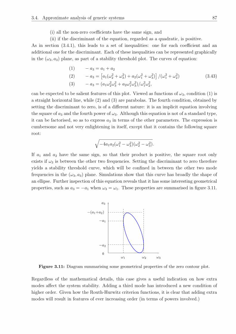
3.4. Approximate analysis of generic systems 87
(i) all the non-zero coefficients have the same sign, and
(ii) if the discriminant of the equation, regarded as a quadratic, is positive.
As in section (3.4.1), this leads to a set of inequalities: one for each coefficient and an
additional one for the discriminant. Each of these inequalities can be represented graphically
in the (ω3, a3) plane, as part of a stability threshold plot. The curves of equation:
(1) − a3 = a1 + a2
(2) − a3 =[a1(ω
22 + ω2
3) + a2(ω21 + ω2
3)]/(ω2
1 + ω22)
(3) − a3 = (a1ω22ω
23 + a2ω
21ω
23)/ω
21ω
22,
(3.43)
can be expected to be salient features of this plot. Viewed as functions of ω3, condition (1) is
a straight horizontal line, while (2) and (3) are parabolas. The fourth condition, obtained by
setting the discriminant to zero, is of a different nature: it is an implicit equation involving
the square of a3 and the fourth power of ω3. Although this equation is not of a standard type,
it can be factorised, so as to express a3 in terms of the other parameters. The expression is
cumbersome and not very enlightening in itself, except that it contains the following square
root:√
−4a1a2(ω21 − ω2
3)(ω22 − ω2
3).
If a1 and a2 have the same sign, so that their product is positive, the square root only
exists if ω3 is between the other two frequencies. Setting the discriminant to zero therefore
yields a stability threshold curve, which will be confined in between the other two mode
frequencies in the (ω3, a3) plane. Simulations show that this curve has broadly the shape of
an ellipse. Further inspection of this equation reveals that it has some interesting geometrical
properties, such as a3 = −a1 when ω3 = ω1. These properties are summarised in figure 3.11.
0
PSfrag replacements
a3
−a1
−a2
ω3ω1 ω2
−(a1+a2)
Figure 3.11: Diagram summarising some geometrical properties of the zero contour plot.
Regardless of the mathematical details, this case gives a useful indication on how extra
modes affect the system stability. Adding a third mode has introduced a new condition of
higher order. Given how the Routh-Hurwitz criterion functions, it is clear that adding extra
modes will result in features of ever increasing order (in terms of powers involved.)

88 Chapter 3. Theory of linear instability in systems with a sliding point contact
The behaviour of this system will now to be simulated. Mode 1 has a frequency 1 and
amplitude 1. Mode 2 has a frequency 1.2 and amplitude 1. Mode 3 has its amplitude varied
from −5 to 0 and its frequency will range from 0.8 to 1.4. As in the two-mode section, the
frequencies have been normalised. The range of variation of the third mode frequency spans
a symmetrical interval around the fixed pole frequencies. As explained in the introduction
to this section, only the poles around a given frequency of interest are assumed to have an
influence on the stability.
In order to condense more information into a single plot, the stability of the system will often
be represented by a surface plot showing the minimum imaginary part of the zeros of D(ω),
as a3 and ω3 are varied. Figure 3.12(a) shows such a plot. The system is unstable whenever
this plots shows a negative value. Figure 3.12(b) shows the contour plot corresponding to
0.8
1
1.2
1.4
−5−4
−3−2
−10
−0.1
−0.05
0
ω3 a
3
Min
. im
agin
ary
part
of
zero
s
(a)
0.8 0.9 1 1.1 1.2 1.3 1.4
−5
−4
−3
−2
−1
0
Third mode frequency
Thi
rd m
ode
ampl
itude
(b)
Figure 3.12: (a) Surface plot showing the minimum imaginary part of the zeros of an un-damped three-mode system where two are kept fixed whereas the third one is varied in am-plitude and frequency. The zero contour line (stability threshold) is shown on the surface andon the base plane. (b) Contour plot of the surface plot shown in (a). The thick line is thezero contour. Thinner lines are the contours for values −0.1, −0.2, −0.5. Note that for bettervisibility, the surface plot has been rotated, so that the origin is the bottom right corner.
the surface shown in (a). The thick line is the zero contour: it is the threshold of stability
of the system. Thinner lines are the contours for more negative values. This plot is the
three-mode version of the plots shown in figure 3.5 with two modes. The horizontal line
at −a3 = a1 + a2 = 2 is clearly visible. The sloping curve across the plot corresponds to
the quadratic condition (3) given above. The curve of elliptical shape corresponds to the
discriminant condition. It is the new, higher order feature introduced by the third mode.
The zero contour is superimposed on the surface plot shown in figure 3.12(a). Giving depth
to the contour plot, this surface plot gives some information regarding the “degree” of in-
stability. Three main parts may be distinguished. First, in the front right of the plot, the

3.4. Approximate analysis of generic systems 89
surface has a cylindrical shape corresponding to the ellipse shape described above. Along
and within this cylinder, the surface dips to relatively modest negative values. Second, the
region near the line where the third pole amplitude is −2 shows a “canyon”. The edges of
this “canyon” correspond to conditions (1) and (3) above. Condition (1), which marks the
passage through zero of the leading coefficient of the quadratic equation (3.42), causes one
of the roots to move from plus to minus infinity at the crossing. This being well off the scale
of this plot, the surface has been limited to show the smooth part of the behaviour. Third,
at the back, left-hand side of the plot, there is a flat surface. This shows that the system is
(marginally) stable for higher values of |a3|.To link these results to the behaviour observed when the third mode was approximated by
a constant residual, it is useful to investigate the individual behaviour of the zeros. This
also helps understand how the surface just described is constructed. Figure 3.13 details the
0.8 0.9 1 1.1 1.2 1.3 1.4−2
−1
0
1
2
Third mode frequency
Rea
l par
t of z
eros
(a) Real parts
0.8 0.9 1 1.1 1.2 1.3 1.4−1
−0.5
0
0.5
1
Third mode frequency
Imag
inar
y pa
rt o
f the
zer
os
(b) Imaginary parts
−1.5 −1 −0.5 0 0.5 1 1.5−0.2
−0.1
0
0.1
0.2
Real part of zeros
Imag
inar
y pa
rt o
f zer
os
(c) Root locus plot
Figure 3.13: Plots showing the behaviour of the zeros when the third mode frequency ω3 isvaried from 0.8 to 1.4, while the third mode amplitude is kept constant at -1.5. (a) shows thereal part of the zeros. (b) their imaginary part. (c) combines (a) and (b) in a root-locus plot.The two crosses in (c) show the position of the poles of the two fixed modes in the complexplane.
behaviour of the roots by showing (a) the real parts of the roots, (b) their imaginary parts.
Plot (c) combines (a) and (b) into a root locus plot. For these three plots, a3 is set to −1.5,
while ω3 is varied from 0.8 to 1.4. This amounts to looking at the roots within a vertical plane
section of the surface plot. This section is marked by a black frame in figure 3.12(a), and
a dashed line on the contour plot (b). In figure 3.13(b), the bottom curve is the minimum
imaginary part within the section, therefore it is the curve that shapes the surface. The
moderate dip between the two fixed frequencies represents a section through the cylinder.
The splitting at the lower end of the frequency range appears as a cliff in the surface plot.
These results agree with the conclusions from the previous approximation, where the third
mode was modelled as a constant residual. Figure 3.13(c) is clearly similar to figure 3.8.
Figures 3.13(a-b) also confirm the previously observed relation between mergings of the
real parts and the occurrence of instability. In the undamped case, the system is unstable

90 Chapter 3. Theory of linear instability in systems with a sliding point contact
whenever the real parts of two modes of the coupled system merge. Mathematically, this is
a direct consequence of the algebraic property (5) listed in section (3.3).
To complete the description of the undamped case, a section for ω3 fixed at 1.1 is taken
across the surface plot shown in figure 3.12(a). The third mode amplitude a3 is varied from
−5 to 0. Figures 3.14(a-b) show respectively the real and imaginary parts of the roots in
this section. These plots show that varying the third mode amplitude significantly affects
−5 −4 −3 −2 −1 0−2
−1.5
−1
−0.5
0
0.5
1
1.5
2
Third mode amplitude
Rea
l par
t of z
eros
(a) Real parts
−5 −4 −3 −2 −1 0−0.4
−0.3
−0.2
−0.1
0
0.1
0.2
0.3
0.4
Third mode amplitude
Imag
inar
y pa
rt o
f the
zer
os
(b) Imaginary parts
Figure 3.14: Plots showing the behaviour of the zeros when the third mode frequency ω3 iskept fixed at 1.1, while the third mode amplitude is varied from -5 to 0. (a) shows the realpart of the zeros. (b) their imaginary part.
the system stability for fairly low absolute values of a3. As mentioned before, there is a
strong “accident” when a3 = −(a1 + a2) = −2, that is, when the leading coefficient of the
polynomial defined by equation (3.42) becomes zero. The bottom curve in figure 3.14(b)
is the minimum imaginary part of the roots within this section. It reveals the shape of a
section at constant ω3 through the cylinder already referred to in the surface plot. When a
similar section is taken through the surface, such that the section does not cross the cylinder,
the variation of the roots is not very different. Whether the section is taken at a frequency
below ω1 = 1 or above ω2 = 1.2, the singularity around a3 = −2 remains. Below ω1, the
behaviour is very similar to that shown in figure 3.14. When ω3 > ω2, the behaviour before
and after that value are “flipped”: what was happening before a3 = −2 in figure 3.14 occurs
after and vice-versa.
Whether the cylinder is crossed or not makes a subtle but important difference. When the
section is taken at a fixed value of ω3 such that the cylinder is not crossed, the roots become
purely imaginary while a3 is in the steep unstable “valley” described in the surface plot
(that is, between the curves defined by conditions (1) and (3) in equation (3.43)). Purely
imaginary zeros could also be observed in the section at constant a3 shown in figure 3.13.
The presence of purely imaginary zeros is somewhat problematic. If the system had only 3

3.4. Approximate analysis of generic systems 91
modes, the model would be exact and the purely imaginary zeros would simply imply that
for those parameter values, the system variables could grow or decay exponentially. However,
the objective of these simulations is rather to approximate locally a complex system by a few
modes. It is possible that purely imaginary zeros may actually exist for a given system, but
it is not possible to tell from the present analysis whether they constitute reliable predictions
or not. Given that the analysis is intended to be local, credit should only be granted to those
roots which lie in the vicinity of the original poles (the two fixed ones at 1.0 and 1.2 as well
as the varying one). The frequency band in which the results can be considered meaningful
has been chosen (somewhat arbitrarily) to range from 0.6 to 1.6 (i.e. ±0.2 the limits of third
pole frequency range). This ‘range of validity’ is indicated in figure 3.13(a) and figure 3.14(a)
by two dashed lines.
Bearing this in mind, the way the surface is plotted can be modified, so that the only
roots included in the calculation of the minimum imaginary part, are those whose real
parts lie within this assumed “range of validity”. Figure 3.15 shows the result when this
procedure is applied. This surface plot shows that the only remaining instability feature is
0.8
1
1.2
1.4
−4−2
0
−0.1
−0.05
0
ω3
a 3
Min
. im
agin
ary
part
of
zero
s
Figure 3.15: Surface plot showing the minimum imaginary part of the zeros of a three-modesystem where two are kept fixed whereas the third one is varied in amplitude between -5 and0 and in frequency between 0.8 and 1.4. Only those roots whose real part lies between 0.6and 1.6 were considered for the computation of the minimum. The zero contour line (stabilitythreshold) is shown on the surface and on the base plane.
the cylindrical sleeve. As a cross-check, the zeros have also been computed using a positive-
pole approximation for D(ω). The result is not shown because the corresponding surface
plot looks exactly the same as figure 3.15. This suggests that this cylindrical feature might
indeed play an important role; an argument which becomes even stronger if one recalls that
the rounded shape in the root-locus plot, characteristic of a section through the cylinder,
was also apparent from the “constant residual” approximation.
In the remainder of this chapter and the next, the procedure consisting in ignoring the
zeros whenever their real part lies outside the range of validity will always be used. This

92 Chapter 3. Theory of linear instability in systems with a sliding point contact
will probably make any analytical prediction of the plot features very difficult; but it seems
essential to the coherence of this work. Once the credibility of the predictions has been
clarified, it is possible to investigate the influence of various parameters on the stability.
First, the influence of varying the values of the modal amplitudes will be discussed.
Influence on stability of varying the modal amplitudes
The expression for the function D(ω) given by expansion (3.12) is a linear combination of ai.
This means that only the relative magnitude and sign of these coefficients matters. In the
simulation results shown so far, the two fixed modes had an amplitude of 1. Since these two
modes play a somewhat interchangeable role, choosing the same value for their amplitude
may lead to misleading conclusions. The purpose of this subsection is to investigate the
effect on stability of three different modal amplitudes. For the results shown next, a1 will
be kept fixed at 1 and a2 will be given various positive values. a3 will sweep [−10 0], so
as to show the most important features. Using the usual format, figure 3.16 shows three
0.8
1
1.2
−10−8
−6−4
−2
−0.1
−0.05
0
ω3
a 3
Min
. im
agin
ary
part
of
zero
s
(a) a2 = 0.1
0.8
1
1.2
−10−8
−6−4
−2
−0.1
−0.05
0
ω3
a 3
Min
. im
agin
ary
part
of
zero
s
(b) a2 = 5
0.8
1
1.2
−10−8
−6−4
−2
−0.1
−0.05
0
ω3
a 3
Min
. im
agin
ary
part
of
zero
s
(c) a2 = 10
Figure 3.16: Surface plots showing the minimum imaginary part of the zeros for variousthree-mode undamped systems, showing the influence of the amplitude values. The parametervalues are as follow: ω1 = 1, a1 = 1, ω2 = 1.2, a2 takes a different value for each plot: (a)0.1, (b) 5, and (c) 10. The third mode is varied in amplitude and frequency within the rangesshown.
surface plots for three different values of a2. From this set of plots, it can be concluded
that the instability features described in the previous section are not significantly altered,
even if very different values are used for the amplitudes. After removal of the unsuitable
zeros, the main instability feature remaining is again the cylindrical shape. The features of
the elliptical cylinder described in figure 3.11 are still valid. This implies that instability is
confined within a rectangle limited by the two fixed frequencies in one direction and the lines
a3 = 0 and a3 = −(a1 + a2) in the other. Consequently, if one of the fixed modal amplitudes
becomes vanishingly small, the ellipse reduces to one of the diagonals of the rectangle. This
is consistent with the fact that the elliptical cylinder is specifically linked to the presence of
a third mode.

3.4. Approximate analysis of generic systems 93
An important conclusion – albeit a negative one – is that a significant variation of the
amplitudes does not add any new feature to the previous description.
The influence of damping
The study of the simpler approximations showed that the damping had a rather subtle
but important effect on stability. Therefore, it is of interest to investigate the influence
of damping on the present three-mode model. To show how damping affects the system, a
particular distribution of damping will be described in some detail, following a similar format
to that used in the undamped case. Several distributions of damping will then be compared.
If modes 1 and 2 are indeed modes of the disc and mode 3, a mode of the brake, it is plausible
that mode 3 has a higher damping than modes 1 and 2. Accordingly, the damping factors
will be: δ1 = 0.01, δ2 = 0.01, δ3 = 0.03. To make comparisons with previous plots easier,
other parameter values will be given the same values as in the undamped case. Mode 1
will have a frequency and amplitude of 1. The frequency and amplitude of mode 2 will be
set at 1.2 and 1 respectively. Mode 3 will be varied in frequency from 0.8 to 1.4, while its
amplitude will cover [−5 0]. Figures 3.17(a-b) show the surface plot resulting from simulating
the behaviour of the three-mode system with these values. Temporarily infringing the rule
0.8
1
1.2
1.4
−5−4
−3−2
−10
−0.1
−0.05
0
a 3
ω3
Min
. im
agin
ary
part
of
zero
s
(a) All zeros included
0.8
1
1.2
1.4
−5−4
−3−2
−10
−0.1
−0.05
0
a 3
ω3
Min
. im
agin
ary
part
of
zero
s
(b) Only “valid” zeros included
Figure 3.17: Surface plots showing the minimum imaginary part of the zeros for a three-mode system with damping. The parameter values are as follows: ω1 = 1, a1 = 1, δ1 = 0.01,ω2 = 1.2, a2 = 1, δ2 = 0.01, δ3 = 0.03, a3 and ω3 are varied within the ranges shown. Thethick line on the surface and bottom plane shows the zero-contour.
previously set, figure 3.17(a) shows the minimum imaginary part of the zeros when all zeros
are included. This is to allow a better comparison with the corresponding undamped case
shown in figure 3.12(a). Damping appears to have distorted the surface, but all the features
previously described can still be recognised. Overall, damping has blunted most of the sharp
edges, and made stable most of the areas previously marginally stable. The cylindrical sleeve
is again an important feature of the plot. The steep valley is still present. The main difference

94 Chapter 3. Theory of linear instability in systems with a sliding point contact
occurs for large negative values of a3. In this area, the surface now slightly slopes down near
the valley. It also has a ridge along the line ω3 = 1.1. Figure 3.17(b) shows the corresponding
surface, when only the zeros whose real parts lie within [0.6 1.6] are considered. As in the
undamped case, the steep valley has disappeared. However, a substantial area of the zone
a3 < −2 is now unstable. It was marginally stable in the undamped case.
Figure 3.18 shows the behaviour of the roots within the section marked by a black frame
in figure 3.17(a). This section is defined by a constant amplitude a3 = −1.5. These plots
0.8 0.9 1 1.1 1.2 1.3 1.4−3
−2
−1
0
1
2
3
Third mode frequency
Rea
l par
t of z
eros
(a) Real parts
0.8 0.9 1 1.1 1.2 1.3 1.4−1
−0.5
0
0.5
1
Third mode frequency
Imag
inar
y pa
rt o
f the
zer
os
(b) Imaginary parts
0 0.5 1 1.5−0.2
−0.1
0
0.1
0.2
0.3
Real part of zeros
Imag
inar
y pa
rt o
f zer
os
(c) Root locus plot
Figure 3.18: Plots showing the behaviour of the zeros of a damped three-mode system, whenthe third mode frequency ω3 is varied from 0.8 to 1.4, while the third mode amplitude is keptconstant at -1.5. The first two modes, shown by a cross in (c), are kept fixed. (a) shows thereal part of the zeros. (b) their imaginary part. (c) combines (a) and (b) in a root-locus plot.The dashed lines in (a) show the range of validity for the real parts.
correspond to those shown in figure 3.13. It can be seen that the behaviour is recognisably
similar. There is still an apparent correspondence between the merging of the real parts and
the dipping of the imaginary part into negative values, but this does not seem as clear as
in the undamped case. These plots also show that, at least when the dip is crossed, adding
damping to the three-mode system has a very similar effect to adding damping to the system
consisting of two modes plus constant.
Several damping distributions are now compared. It is easier to make this comparison by
showing zero contour plots. Figure 3.19 shows such plots for four different distributions given
in the figure caption.
Many other distributions of damping have been investigated. The plots shown are represen-
tative. These particular cases are shown because one of them, (b), has just been studied
in detail. Cases (c) and (d) are simply permutations within the three modes of the same
damping factor values.
From these plots and others not shown, some important conclusions can be drawn:
(1) As noted for the two-mode approximation, when the distribution of damping is
uniform (i.e. plot (a)), the stability threshold is the same as in the undamped case. For the
case shown, the damping factors were all set to 0.01.

3.4. Approximate analysis of generic systems 95
0.8 0.9 1 1.1 1.2 1.3 1.4
−5
−4
−3
−2
−1
ω3
a 3
(a) δ1 = 0.01, δ2 = 0.01, δ3 = 0.01
0.8 0.9 1 1.1 1.2 1.3 1.4
−5
−4
−3
−2
−1
ω3
a 3
(b) δ1 = 0.01, δ2 = 0.01, δ3 = 0.03
0.8 0.9 1 1.1 1.2 1.3 1.4
−5
−4
−3
−2
−1
ω3
a 3
(c) δ1 = 0.01, δ2 = 0.03, δ3 = 0.01
0.8 0.9 1 1.1 1.2 1.3 1.4
−5
−4
−3
−2
−1
ω3
a 3
(d) δ1 = 0.03, δ2 = 0.01, δ3 = 0.01
Figure 3.19: Plots showing contour lines of the minimum imaginary part surface for differentdistributions of damping. The thick line is the zero-contour. Thinner lines are for morenegative values. The two fixed modes had parameters set as follows: ω1 = 1, a1 = 1, ω2 = 1.2,a2 = 1.
(2) Whatever the distribution of damping, the cylinder described in the undamped case
appears to be a significant and extremely robust feature. It was shown in the undamped case
that this feature occurs for values of a3 between 0 and −(a1 + a2). The stability thresholds
for larger negative values of a3 is more variable. This is probably due to the relative flatness
of the surface in this region: a small variation of the position of the surface can result in a
large shift in the threshold line.
(3) It seems that the unstable region is larger, whenever the damping is not uniformly
distributed. This suggests that, from a stability point of view, a uniform distribution of
damping is optimum.

96 Chapter 3. Theory of linear instability in systems with a sliding point contact
(4) The damping affects the stability boundary very significantly and in a non-systematic
way. Slight modifications of the damping within a system can result in a very different sta-
bility map. This may be one of the reasons for the “capriciousness” of friction-induced
vibration phenomena. It is difficult to believe that the natural frequencies or mode shapes
of a particular system will change significantly if only minor modifications are made. How-
ever, it is plausible that tightening a bolt, or adding a shim, can sightly alter the damping
mechanisms within the system, causing it to become stable or unstable.
Throughout this chapter, the damping is assumed to be proportional. The influence of non-
proportional damping will be discussed in the next chapter. The next section reviews the
concept of mode locking in the light of the conclusions reached so far.
Mode-locking
Mode-locking is the name of a common natural phenomenon which occurs when two damped
oscillators vibrating with very close frequencies are weakly nonlinearly coupled. In these
conditions, the frequencies of the two oscillators become strictly identical. This mechanism
is used to explain the synchronisation of the moon on the Earth’s rotation, so that the moon
always shows the same face to a terrestrial observer (Berger et al. (1984)). In the brake
noise context, the phrase “mode locking” is used to mean that instability is more likely to
occur when two natural frequencies of the uncoupled subsystems are very close. Whether
this particular use of the phrase by the brake noise community means the same as the more
general phenomenon described above is not clear2. In practice, this rule is often used to
rapidly assess where squeal might occur. Even with this restricted purpose, it only has
a limited value: a brake assembly consists of many different parts of comparable size and
mass, so that components are likely to possess a number of close natural frequencies, few
of which will actually be squealing frequencies. Allgaier et al. (2001) used this phrase in
a study on brake noise but generally speaking, it has received fairly little attention from
the brake research community and scarce evidence has been produced, either supporting or
invalidating the claim.
Whether brake noise is related to general mode locking or not, the present analysis sheds
a new light on the rule of thumb used by brake manufacturers. The simulation results
presented in this chapter suggest that with only two modes, instability is not influenced by
the closeness of the two natural frequencies. With three modes, it appears that the most
robust feature is the shallow dip showing in the surface plots in the damped case, or the
cylindrical sleeve in the undamped case. In all simulation results shown, the imaginary part
reaches its most negative value when the third mode frequency equals 1.1 (that is mid-way
between the two fixed mode frequencies) and when the third mode amplitude equals −2
2Given the first general definition given above, it would appear that experimental brake squeal fits thedescription quite well: two close modes of the separate subsystem would lock onto each other at a squealfrequency. At face value however, it looks as if the type of analysis presented in this chapter and the previousone has very little in common with general mode locking, since here, instability (and not synchronisation) ispredicted using a purely linear theory.

3.4. Approximate analysis of generic systems 97
(that is when the amplitudes add up to zero). This qualifies the concept of ‘mode locking’:
the most general conclusion that can be drawn from this analysis is that instability is more
likely to arise when three consecutive modes have fairly close frequencies ω1 < ω2 < ω3, whose
corresponding modal amplitudes3 have alternating signs: +−+ or, less probably, −+−. The
study of the three-mode approximation suggests that the coincidence of two frequencies is a
significant property. However, it does not indicate that instability is more likely. Rather, it
often marks the limit between stability and instability. It also appears from observation of
the real part plots (e.g. in figure 3.18(a)), that when the pattern just described is unstable,
the unstable frequency of the combined system is very close to the middle frequency ω2. It is
also interesting to note that in this analysis, no distinction is made regarding the origin of a
particular mode: once the system is coupled by friction, the modes which possess a positive
“modal amplitude” in D, form a pool of equivalent interacting “modal terms”, regardless of
which subsystem they originate from. As already mentioned, “modal terms” with negative
amplitudes can only arise from the brake, if the disc is perfectly symmetrical.
This completes the study of the three-mode approximation. The array of behaviours resulting
from the presence of a third mode proved to be much richer and irreducible to the behaviour
exhibited by only two modes. The next section investigates whether the addition of other
modes again results in such drastically different behaviours.
3.4.4 Influence of additional modes
The previous section points toward the important influence on stability of particular three-
mode sequences. In order to investigate how much of the previous conclusions hold when
the three modes are included in a more complex system, a fourth relatively remote mode
is added to the system studied in the previous section. Two cases will be studied: (1) the
extra mode amplitude will have the same sign as that of the varying mode, (2) it will have
the opposite sign, i.e. the same sign as the fixed modes.
Figure 3.20(a) is the usual surface plot showing the minimum imaginary part of a four-mode
system. For this simulation run, the first two modes were given the same properties as
those used for the results shown in figure 3.17, that is, frequencies at 1 and 1.2 and both
amplitudes set to 1, damping factors 0.01 for the first two modes. The extra fourth mode
was given a frequency 2, amplitude -1, and damping factor 0.01. The third mode is again
varied in frequency from 0.8 to 1.4, and in amplitude from -5 to 0. Its damping factor was
set to 0.03. Figure 3.20(b) shows the corresponding zero-contour. For these two plots, only
the roots whose real parts are within 0.6 and 1.6 are considered to compute the minimum.
It appears that the behaviour described in the previous section is only moderately affected
by the extra mode. Comparing figure 3.17(b) and figure 3.20(a), the main difference is the
appearance of a sector dipping steeply into negative values when the varying frequency is
below 1 and a3 around −3. Except for this new unstable zone, the rest of the plot is almost
3Here, it might be useful to recall that the phrase “modal amplitude” refers to the numerator of theresonant terms in D(ω) and not to the amplitude of any mode as such.

98 Chapter 3. Theory of linear instability in systems with a sliding point contact
0.8
1
1.2
1.4
−5−4
−3−2
−10
−0.1
−0.05
0
ω3
a 3
Min
. im
agin
ary
part
of
zero
s
(a)
0.8 0.9 1 1.1 1.2 1.3 1.4−5
−4
−3
−2
−1
0
ω3
a 3
(b)
Figure 3.20: (a) Surface plot showing the minimum imaginary part of the zeros for a systemcontaining 3 fixed modes with frequencies 1, 1.2, 2 amplitudes 1, 1 and −1, while a third modeis varied in frequency and amplitude. (b) Zero-contour of the surface plot on the left.
identical to the corresponding three-mode plot. In particular, the round shallow dip is hardly
affected. Other simulations show that, as the extra mode moves away (i.e. ω4 moves away
from 1), the unstable sector gradually becomes a narrow, steep “valley”, along the straight
line characterised by a constant amplitude equal to −2. This shows that an isolated cluster
of three modes indeed behaves as described in the previous section.
Figures 3.21(a-b) show the corresponding data when the sign of the fourth mode amplitude
is made positive. At first sight, it appears that the influence of the extra mode with negative
residue is similar to that previously described, except that it is now the instability band on
the right hand side of the contour plot which has become wider. The round shallow dip is
again remarkably robust. However, closer investigation shows that changing the sign of the
fourth modal amplitude causes the two systems to behave differently in a more fundamental
way.
In the previous section, it was concluded that the stability behaviour of a three-mode system
is strongly dependent on the sign of the modal amplitudes. It was shown that instability
can only occur if these signs alternate, and that instability is likely to arise when this con-
dition is satisfied and when the negative amplitude has moderate values (typically below
the opposite of the sum of the other amplitudes). When an extra mode is added, there are
several possibilities to group the modes by clusters of 3. Table 3.1 summarises the various
configurations depending on the position of ω3 and the sign of the fourth mode amplitude,
a4. This table shows how the sign patterns change as the third mode frequency, ω3, varies.
Note that the amplitude of this varying mode is kept negative for both positive and negative
values of a4. The clusters of signs appearing in the table are the signs of the amplitudes

3.4. Approximate analysis of generic systems 99
0.8
1
1.2
1.4
−4
−2
0−0.1
−0.05
0
ω3 a
3
Min
. im
agin
ary
part
of
zero
s
(a)
0.8 0.9 1 1.1 1.2 1.3 1.4−5
−4
−3
−2
−1
0
ω3
a 3
(b)
Figure 3.21: (a) Surface plot showing the minimum imaginary part of the zeros for a systemcontaining 3 fixed modes with frequencies 1, 1.2, 2, amplitudes +1, +1, and +1, while a thirdmode is varied in frequency and amplitude. (b) Zero-contour of the surface plot on the left.
ω3 1 1.2 3
a4 < 0 − + +− [+−+]− + + −− + + −−
a4 > 0 − + ++ [+−+]+ +[+−+] + + +−
Table 3.1: Table showing the various sign patterns as the third mode frequency is varied.The sign corresponding to this mode is shown in bold. a4 denotes the extra fourth modeamplitude. The square brackets highlight the clusters expected to lead to instability.
ordered by increasing frequency. Thus, if ω3 < ω1 = 1, and a4 > 0 (top left cell), then the
first sign corresponds to the sign of a3, i.e. minus. The second sign (+) corresponds to the
sign of a2, the second mode encountered in increasing frequency, and so on. As ω3 is var-
ied and passes through the various fixed mode frequencies, the sign sequence changes. The
main objective here is to investigate if the conclusions reached in the previous section for
a three-mode model are still valid for a cluster of three modes forming part of a four-mode
system. The potentially unstable clusters of three modes are shown within square brackets
in the table; they are the ones with three consecutive alternating signs.
Figure 3.22 contains two surface plots showing the minimum imaginary part of the roots for
the two previous four-mode systems. The only difference with figures 3.20 and 3.21 is that
the variable mode has been allowed to vary over a frequency range covering the fourth fixed
modes as well, i.e. ω3 ranges from 0.8 to 2.4. The extra fourth mode again has its frequency
set at 2, its damping factor equals 0.01 and its modal amplitude is set to −1 in figure 3.22(a)
and +1 in figure 3.22(b). It is not surprising that figure 3.21(a) and figure 3.22(a) have show

100 Chapter 3. Theory of linear instability in systems with a sliding point contact
0.81
1.21.4
1.61.8
22.2
−5−4
−3−2
−10
−0.1
−0.05
0
ω3 a
3
Min
. im
agin
ary
part
of
zero
s
(a) a4 < 0
0.81
1.21.4
1.61.8
22.2
−5−4
−3−2
−10
−0.1
−0.05
0
ω3
a 3
Min
. im
agin
ary
part
of
zero
s
(b) a4 > 0
Figure 3.22: Surface plot showing the minimum imaginary part of the zeros for a four-modesystem containing 2 fixed modes with frequencies 1, 1.2, amplitudes 1, while a third mode isvaried in frequency and amplitude. The fourth mode is added with frequency 2 and amplitude(a) a4 = −1 (b) a4 = +1.
similar features in the lower frequency range, since these plots are identical, except for the
larger range of variation of the third mode frequency in figure 3.22. These two plots clearly
show that the conclusions drawn from table 3.1 are valid when the third mode amplitude is
between 0 and −2. As expected, if a4 > 0, instability arises when the varying mode frequency
lies within 1 and 2, that is between the two extreme fixed frequencies. When a4 < 0, the
system is only unstable when the varying frequency is within 1 and 1.2. Figure 3.22(b)
is particularly interesting as it shows that each cluster of three alternating signs behaves
somewhat independently: the plot in the [1.2 3] frequency range appears to be a magnified
version of the plot in the [1 1.2] range. Thus, adding an extra mode has simply duplicated
the behaviour described for a three-mode system, at least for the most robust part, i.e., when
all the residues have comparable absolute values. Note that the behaviour is more complex
when a3 < −3, where the system exhibits a strong fickleness of behaviour. However, it should
be kept in mind that such large negative values are rather unlikely to arise in practice.
To conclude this simulation section, figure 3.23 shows the plot of the imaginary part against
the real part of the roots in the section taken from the surface plot 3.22(b), defined by
a3 = −1, while ω3 is varied from 0.8 to 2.4. This figure clearly shows that with more
than three modes, the behaviour described in the three mode section (e.g. in figure 3.18(c)),
repeats itself within each cluster of three modes. Figure 3.18(c) is actually a zoom around the
lower two fixed modes in figure 3.23. This root locus plot also suggests that the dimensions
of the loop that goes into the unstable half of the complex plane are connected to the interval
separating these two fixed mode frequencies (this is clear in the undamped case, as seen from
figure 3.11). Therefore, instability might be stronger for clusters of 3 modes with amplitudes
of alternating signs and fairly widely spaced frequencies.

3.5. Conclusions 101
0.5 1 1.5 2 2.5
−0.2
−0.1
0
0.1
0.2
0.3
Real part of zeros
Imag
inar
y pa
rt o
f zer
os
Figure 3.23: Root locus plot for the four-mode system described in figure 3.22(b). This plotshows that the behaviour of a three mode system, as shown in figure 3.18(c), is essentiallyduplicated when the system contains more modes. The crosses represent the position of thefixed poles in the complex plane.
3.5 Conclusions
The modelling presented in this chapter allows stability to be investigated for any system
containing two linear subsystems in sliding contact at a single point. The mechanical be-
haviour of the two contacting subsystems is captured via a set of transfer functions at the
contact point, regardless of their physical realisation. Assuming the damping is proportional,
these transfer functions can in turn be expressed in terms of eigenfrequencies, damping fac-
tors and mode shapes. Using Coulomb’s law with a constant coefficient of friction to model
the friction behaviour at the interface, the following conclusions were reached:
1. For such a system to be unstable, it is necessary that the system possesses some
asymmetry so that, at least for one of the subsystems, the normal and tangential
degrees of freedom are dynamically coupled.
2. It is also necessary that at least one of the “composite modal amplitudes” appearing
in expansion (3.12) becomes negative. Larger values of the coefficient of friction help
to reach such negative modal amplitudes.
3. For a three-mode undamped system, instability was shown to arise if and only if the
composite modal amplitudes satisfy a certain pattern of signs. If this is so, instability
will occur within a definite region in the parameter space.
4. For a damped three-mode system, damping will in general make the system stable
when the corresponding undamped system is stable. Provided damping is light, the
stability boundaries of the undamped system are only moderately affected, so that the
stability domain is usually recognisable. However, damping can also cause substantial
new unstable regions of the parameter space to appear. The exact topography of

102 Chapter 3. Theory of linear instability in systems with a sliding point contact
these unstable regions is highly unpredictable and it strongly depends on the damping
distribution. The less uniform the damping in the system, the wider the instability
domain of the damped system is likely to be. This suggests that damping is one of the
reason for the capriciousness of systems containing a sliding point contact.
5. Many features of systems with more than 3 modes can be understood by viewing them
as consisting of fairly independent clusters of 3 modes. Therefore, the conclusions
reached from the three-mode system analysis can be used for any other system to
a reasonable extent. This justifies a posteriori the appropriateness of using a local
approximation for the study of stability.
A major strength of the present modelling is that the theory proposed is inherently non-
controversial. When instability is predicted by this linear theory, one would expect something
to be observed. It is therefore important to review all the plausible features that might
influence stability within linear theory. This is the object of the next chapter.

Chapter 4
Extensions of the linear model
4.1 Introduction
The theory presented in Chapter 3 allows the modelling of a general class of systems con-
taining a frictional contact. The conclusions drawn from this theory rely on the following
assumptions:
• The dynamics of the two subsystems in contact is linear.
• The subsystems are in a steady-sliding regime.
• Sliding results from the motion of one or both subsystems. The bulk motion of the
moving subsystem(s) does not alter significantly its/their dynamical properties mea-
sured at rest.
• Sliding occurs at a single location with no geometrical extension (single point contact).
• The contact between the two subsystems is not compliant.
• The damping is proportional so that the modes of the two subsystems can be described
by real mode shape coefficients.
• The relation between the friction force and the normal force can be appropriately
described by a coefficient of friction which is independent of any other working variable.
Chapter 3 can be regarded as a study of the simplest possible case. It was dealt with in
some detail and will serve as a reference. In the present chapter, the scope of the theory is
extended by relaxing some of these assumptions. Some hypotheses cannot be relaxed easily.
For instance, allowing the dynamics to be nonlinear (i.e. relaxing (1)) would fall outside
the scope set in Chapter 1. Therefore, the assumption of linearity will be considered valid
throughout this chapter too.
(2) and (3) can be empirically or practically motivated: squeal mainly occurs at very low
speeds (which supports (3)) and in a vast majority of cases it indeed occurs in systems in
steady sliding.
103

104 Chapter 4. Extensions of the linear model
Relaxing assumption (4) would be difficult if it is understood as implying line contact or
planar contact. However, it is possible to extend the theory of Chapter 3 by reformulating
with two contact points. The algebra is much more complex and the study of the stability
will be the object of further research. A brief outline will be presented in the final chapter.
Therefore, this thesis will mainly deal with a single point contact.
This leaves assumptions (5), (6) and (7). These will be relaxed in turn. For each assumption
relaxed, a new stability criterion will be derived and investigated by simulating the behaviour
of generic systems.
Relaxing assumption (5). First, the system studied in chapter 3 can be modified by
allowing the contact to be compliant. This can be modelled by a linear contact spring between
the points of the two subsystems previously in contact. Whether the theory presented in
chapter 3 already includes the possible dynamic effect of a contact compliance within the
transfer functions is arguable. However, a transfer function with the standard form taken
in equation (3.12) implicitly assigns a mass to each degree of freedom. Therefore, such a
formulation cannot account for a massless spring, free at one end. This can be done using
standard linear system techniques as will be seen next.
Relaxing assumption (6). The second extension investigated is the non-proportionality
of the structural damping. To our knowledge, this has never been mentioned as a possible
source of instability in friction-induced vibration studies. However, if the structural damping
is non-proportional, transfer functions take a slightly different form and it will be shown that
this can affect the stability of the system in an unexpected way.
Relaxing assumption (7). In chapter 3, the stability criterion was derived by modelling
the contact interaction by a constant coefficient of friction. In the present chapter, this
assumption will be relaxed and the coefficient of friction will be allowed to vary. As mentioned
in Chapter 1, a coefficient of friction decreasing with the sliding speed was long thought to
be the main source of unstable friction-induced vibration. It is now generally agreed that
this is probably not the only cause of instability, however the influence of such a feature
is still of interest. For definiteness, the theory will be presented for a coefficient of friction
varying linearly with the sliding speed. However, it will be seen that many other friction
laws, once linearised, would take a similar form, so that the conclusions can apply to a much
more general class of systems.
4.2 Influence of contact compliance
Before studying how contact compliance influences our model, it is useful to recall the basics
of Hertz theory, since it is within this framework that the notion of contact stiffness is best
defined (Johnson (1985)).

4.2. Influence of contact compliance 105
4.2.1 Background on contact compliance
Assuming that a single spherical asperity made of a linearly elastic material is pressed on a
rigid smooth flat plane, Hertz showed that the normal compliance law takes the form:
N = Aδ3/2, (4.1)
where N is the normal load, A a coefficient of proportionality depending on the geometry and
the mechanical properties of the sphere, and δ is the surface separation. Thus, Hertz’ theory
predicts a nonlinear normal compliance law. Provided the load does not vary significantly,
this law can be linearised around the operating load value. The contact stiffness can then
be defined as the coefficient of proportionality between N and δ in this linearised law. The
generalisation of such a law to extended areas of contact between rough surfaces is a difficult
problem. In general, a statistical characterisation of the surface is necessary. Greenwood and
Williamson (1966) gave a solution assuming a Gaussian peak height distribution. However,
throughout this work a point contact is assumed, so the issue does not arise.
Some authors have suggested that contact compliance may have an effect on the stability of
systems in sliding contact. Interest in this area actually stems from two different concerns.
The first originates from a seminal paper by Tolstoı (1967), in which it is suggested that there
is no essential difference between kinematic and static friction. The apparent distinction
is due to the influence of normal vibration superimposed on the tangential vibration. A
number of authors (Martins et al. (1990), Hess and Soom (1991a,b)) have developed this
idea further. If the normal contact compliance is nonlinear, of Hertz type, the waveform of
normal oscillations will be significantly non-symmetrical and such that the average ‘dynamic
penetration’ of the contacting surfaces will be smaller than the static ‘penetration’. This
would produce a slight lifting-up of the slider, which in turn results in a reduction of the
real contact area, thus reducing the coefficient of friction. This mechanism explains how a
nonlinear contact compliance can result in an apparent drop in the friction coefficient in a
dynamic regime. For more detail see (Martins et al., 1990, pp36-38).
The other interest in contact compliance in relation to friction instability arises from its use
as a convenient device in computational studies. When a brake assembly, for instance, is
modelled by finite elements, it is convenient to include contact springs between contacting
nodes. By this device, the normal contact force is simply the product of the contact spring
stiffness by the node distance. The friction force is then simply obtained by multiplying the
normal force and the coefficient of friction (Liles (1989), Ghesquiere (1992), Nack (2000)).
Giving a sufficiently large value for this contact stiffness (typically 106 N/m) also ensures
that the surfaces in contact do not penetrate. Within this context, the contact stiffness
becomes a parameter which can be varied like any other and it is possible to investigate its
influence on stability. This section follows this line of argument.

106 Chapter 4. Extensions of the linear model
4.2.2 Addition of a contact stiffness to the linear model
Adding a linear contact spring between the two subsystems poses no difficulty for the model
presented in chapter 3. In figure 4.1, a normal contact spring kn has been included at the tipPSfrag replacements
‘Disc’ ‘Brake’
Dis
cR
otat
ion
kcv1
u1
u2
v2
u′2
v′2① ②
Figure 4.1: The two previous linear systems now in contact through a contact spring.
of the ‘brake’. This spring could equally well have been attached to the disc, or two different
contact springs could even be attached at the contacting end of each subsystem. u′2 and v′2
represent the displacement of the brake tip in the direction shown, while u2 and v2 represent
the displacement at the end of the contact spring that will now be in contact with the disc.
For clarity, the forces are not represented on this picture. With the same notations and sign
conventions as in Chapter 3, there are equal and opposite normal and tangential forces N ′
and F ′ at the new contact point. These forces are transmitted directly through the massless
spring. The dynamics of the two subsystems ‘disc’ and ‘brake’ considered independently are
again represented using the matrices of transfer functions previously defined. If the contact
region is compliant in the normal direction and if that compliance matters for stability, there
is no reason to believe that the same will not be true in the tangential direction (Ouyang
et al. (1999), Liang and Feeny (1998), Johnson (2000)). Therefore, a contact spring in the
tangential direction kt will also be included in the analysis, although this is not shown on
figure 4.1 to prevent overloading. Following Soedel (Soedel (1981)) or Bishop and Johnson
(Bishop and Johnson (1960)), the contact springs and the ‘brake’ can be viewed as two linear
systems in series. The relationships among forces and displacements defined in figure 4.1
are:
N ′ = kn(u2 − u′2)= kn(u2 −H11N′ −H12F
′) (4.2)
F ′ = kt(v2 − v′2) = kt(v2 −H21N′ −H22F
′). (4.3)
The dynamics of the subsystem ‘brake’ coupled with the contact springs can then be ex-
pressed from the new contact point via the matrix H′ defined as:
[u2
v2
]
= [H′]
[N ′
F ′
]
=
[H11(ω) + 1
knH12(ω)
H21(ω) H22(ω) + 1kt
] [N ′
F ′
]
(4.4)

4.2. Influence of contact compliance 107
In this formulation, it is assumed that the contact compliance does not induce any cross-
coupling term between the normal and tangential directions. With H′ thus defined, the
process outlined in section 3.2 can be applied in exactly the same way. Assuming a constant
coefficient of friction, the conclusion is now that the fully coupled system is unstable if and
only if the function
D(ω) =1
kn
+1
kt
+G11 + µG12 +H11 + µH12 (4.5)
has at least one zero in the lower half ω-complex plane. Before investigating the effect of the
extra term from simulation results, some general comments can be made.
First, it appears from equation (4.5) that the normal and tangential compliances have an
equivalent influence on stability. This justifies a posteriori the assumption that if a normal
spring is included, a tangential one should too.
It is also interesting to examine how the contact stiffness term alters the expected number
of zeros of D. Assuming proportional damping, D(ω) can again be expressed in terms of the
real mode shapes, natural frequencies and damping factors of the two uncoupled subsystems.
This yields an expression for D(ω) similar to expansion (3.12). When the contact stiffnesses
are not included, it was shown in section (3.3) that a system containing Ntot modes in
total when the subsystems are uncoupled, possesses Ntot − 1 modes when the subsystems
are coupled. Now, the same initial Ntot modes give a total of Ntot modes for the coupled
system, as can be seen by putting the terms in D to the same denominator. If both positive
and negative frequency poles are included in the analysis, this indicates that an extra pair
of complex conjugate zeros has appeared, intuitively representing the “contact resonance”.
The reason is that the two “masses” at the original contacting points are no longer merged
into a single “mass” but remain as separate degrees of freedom.
Another point deserves some discussion. In Chapter 3, the absolute magnitude of the am-
plitude coefficients (that is the an , the coefficient at the numerator of each resonant term in
the expansion (3.13)) was not an issue. It is clear from the expression of D in equation (3.13)
that only their relative sign and magnitude mattered. In this section however, the addition
of a constant stiffness term introduces an ‘absolute’ reference in terms of magnitude. It
is useful to carry out a simple order-of-magnitude analysis, in order to estimate plausible
values to be used in the subsequent simulations. Assuming that 1kg is a plausible value
for the modal mass of a typical brake system, then, to a normalised natural frequency of
1, corresponds a non-dimensional structural stiffness of order unity too. Thus, the values
chosen for the contact stiffness in the following simulations will have to be consistent with
the order of magnitude of the structural stiffness.
4.2.3 Simulation results
Some simulation results will now be described. For easier comparisons and connections with
the previous results, a contact compliance is added to the three-mode system investigated
in Chapter 3, section (3.4.3).

108 Chapter 4. Extensions of the linear model
Figure 4.2 is a sequence of surface plots of the minimum imaginary part of the zeros for
systems consisting of three modes plus contact compliance, characterised by the “equivalent”
contact stiffness ke = ktkn/(kt + kn). In this figure, ke is allowed to take four different
values: 100, 10, 1, 0.1. To each value corresponds a surface plot. Amongst the three modes
constituting the system, two are fixed with frequencies 1 and 1.2, damping factors 0.01, 0.01
and both amplitudes equal to 1. The third mode is varied in frequency within 0.8 and 1.4,
and in residue within −5 and 0. Its damping factor is 0.03. Following the notations defined
in Chapter 3, the natural frequency and amplitude of the varying third mode will be denoted
ω3 and a3 respectively. On each surface plot, the zero contour is plotted with a thick line on
the surface itself. This contour is also plotted on the bottom plane using a thick line. As
before, the minimum imaginary part is taken among those roots whose real part is within
the range of validity [0.6 1.6].
Figure 4.2 shows that as the value of the equivalent contact compliance ke decreases, its
influence on the system stability becomes more and more pronounced. For ke = 100, the
zero-contour, visible on the surface in figure 4.2(a) is indeed very similar to figure 3.17(b),
where ke can be considered infinite. This is not surprising since ke only affects the function
D(ω) through its inverse 1/ke, so that relatively large values of ke will only have a slight
effect on the stability.
It also appears that the main effect of the contact compliance ke is to initiate a steep “valley”
spanning the higher range of the third mode frequency and approximately centred on the
line a3 = −2. This valley becomes wider and wider as ke decreases, gradually deforming the
higher quadrant of the surface plot (larger values of ω3 and |a3|). Note that the half of the
surface corresponding to the lower frequency range is little affected, even for small values of
ke.
To understand how the extra mode introduced by the contact compliance modifies the un-
derlying three-mode system, it is useful to examine the individual behaviour of the roots
in a section of one of the surface plots. This is shown in figure 4.3, where the real (a) and
imaginary (b) parts of the roots are plotted against the third mode frequency, a3 being kept
constant at −1.5. For these two plots, ke was set to 1. This corresponds to a section of
the surface plot, represented by a black frame in figure 4.2(c). As can be expected from
equation (4.5), the real parts form equal and opposite pairs, and to each of these pairs corre-
sponds a single imaginary part (if the zero is not purely imaginary). The horizontal dashed
lines in figure 4.3(a) represent the range of validity ([−1.6 −0.6] and [0.6 1.6]), within which
the prediction is considered valid. The roots plotted as triangle (.) and circle () lines are a
slightly distorted version of the roots for a three-mode system without contact compliance.
They correspond to the imaginary parts plotted in figure 3.18(a-b). The slight dipping into
negative values of the root plotted with triangles is part of the rounded dip in the surface
plot. The new imaginary part, coming from the extra pair of roots is plotted with (blue)
crosses (×). From figure 4.3(b), it is clear the latter imaginary part overtakes the triangle
line for higher values of the third mode frequency, thus modifying the surface plot in this
upper frequency range, so as to create the steep “valley”.

4.2. Influence of contact compliance 109
0.8
1
1.2
1.4 −5 −4 −3 −2 −1 0
−0.1
−0.05
0
a 3
ω3
Min
. im
agin
ary
part
of
zero
s
(a) ke = 100
0.8
1
1.2
1.4 −5 −4 −3 −2 −1 0
−0.1
−0.05
0
a 3
ω3
Min
. im
agin
ary
part
of
zero
s
(b) ke = 10
0.8
1
1.2
1.4 −5 −4 −3 −2 −1 0
−0.1
−0.05
0
a 3
ω3
Min
. im
agin
ary
part
of
zero
s
(c) ke = 1
0.8
1
1.2
1.4 −5 −4 −3 −2 −1 0
−0.1
−0.05
0
a 3
ω3
Min
. im
agin
ary
part
of
zero
s
(d) ke = 0.1
Figure 4.2: Surface plots showing the minimum imaginary part of the zeros for systemsconsisting of three modes and a contact frequency term varied as shown. Two of the modesare fixed, while the third one is varying in frequency and amplitude. The bottom of theseplots has been clipped at 0.1 to make important features more visible. The thick line plottedon the surface is the zero contour. This contour is also reproduced on the bottom plane.
As well as setting an absolute reference in magnitude in D(ω), the presence of ke also sets a
reference in sign. Of course, ke is always positive. As far as the zeros of D(ω) are concerned,
giving a negative value to ke in equation (4.5) simply amounts to reversing all the amplitude
signs. Such a sign reversal has no effect on stability if there is no contact compliance. With
contact springs however, this sign reversal matters. Simulations show that it makes the steep
“valley” described above, appear in the lower frequency range of the third mode, rather than
in the upper range. This is reminiscent of the effect of an additional fourth mode on a three-
mode system described at the end of Chapter 3. In section 3.4.4, it was observed that
reversing the sign of the fourth mode amplitude also switched the effect from the lower to
the upper range of the third mode frequency. Furthermore, the influence of the extra mode

110 Chapter 4. Extensions of the linear model
0.8 0.9 1 1.1 1.2 1.3 1.4−2
−1.5
−1
−0.5
0
0.5
1
1.5
2
Third mode frequency
Rea
l par
t of z
eros
(a) Real Parts
0.8 0.9 1 1.1 1.2 1.3 1.4
−0.4
−0.2
0
0.2
0.4
0.6
Third mode frequency
Imag
inar
y pa
rt o
f the
zer
os
(b) Imaginary Parts
Figure 4.3: (a) Real and (b) imaginary parts of the roots against the third mode frequencywhen ke = 1 and the third mode amplitude is fixed at -1.5. The horizontal dashed lines in (a)represent the range of validity [−1.6 − 0.6] and[0.6 1.6]. Some of the roots have been plottedwith specific markers to make individual reference to them in the text easier.
was also described as introducing a steep instability sector, becoming a narrow valley as the
mode moved away. This similarity is not fortuitous. In section (3.4.2), where the influence
of remote poles, modelled as a constant residual was investigated, it was argued that far
away from a mode natural frequency, the influence of this mode could be modelled as a real
constant. Mathematically, this is precisely what the contact stiffness term in equation (4.5)
amounts to. Therefore, it is not surprising that the influence of a compliant contact bears a
strong similarity with the influence of a remote mode. As the equivalent contact stiffness ke
becomes smaller, its inverse increases in magnitude. So, one should not expect this similarity
to hold since the approximation of a neighbouring mode by a constant residual term may no
longer be accurate. However, the striking similarity between figure 4.2(c) and figure 3.20(a)
shows that the contact stiffness term behaves like an extra mode even for stiffness values
comparable with the system structural stiffness. This is a remarkable result.
4.2.4 Conclusions on the influence of contact compliance
In this section, a contact compliance was added to the linear formulation presented in Chap-
ter 3. This compliance was modelled by tangential and normal linear springs. A new
expression for the function D(ω) governing the stability of the coupled system was obtained.
Simulated examples show that a contact compliance significantly affects the system stability
when the value of the contact stiffness is of the same order or below the order of magnitude
of the structural stiffness. If the contact stiffness takes a value of this order of magnitude,
then, to a good approximation, its effect on the system is similar to that of a remote extra
mode.
4.3. Influence of non-proportional damping and complex modes 111
4.3 Influence of non-proportional damping and com-
plex modes
If the damping in either or both subsystems is not extremely small, there is another effect
which can influence the threshold of stability. So far, proportional damping has been assumed
throughout the system, so that the mode shapes are real. However, although this assumption
is very commonly made, the condition of proportional damping is an artificial one, made
purely for mathematical convenience. There is no physical reason to expect most real systems
to conform to this assumption. Instead, one must expect mode shapes to be complex in
general. For most purposes of vibration modelling this distinction matters little, but for
stability analysis it can be very important since it introduces phase shifts. Unfortunately,
there is no universal predictive theory of structural damping which has the same convincing
physical justification as the treatment of stiffness and inertia through stiffness and mass
matrices. The best that can be said is that if the damping is governed by linear theory
and is light, then a perturbation approach can be used to obtain approximations to the
complex frequencies and mode shapes. Surprisingly, it turns out that the expressions for
transfer functions are closely analogous to those used in equation (3.10-3.11). Specifically,
approximations like equation (3.17) take exactly the same form, provided the mode shapes
appearing in equation (3.18) for the coefficients are replaced by their approximate complex
equivalents (Woodhouse (1998)).
It is not usually possible to predict the complex mode shapes from an a priori model of a
system, but at least it is possible to measure them. The techniques of experimental modal
analysis can be applied in the standard way (Ewins (1984)), and provided a sufficiently
sophisticated signal-processing method is used, complex mode shapes can be extracted.
It is of interest to examine briefly the effect of complex mode shapes on the threshold of
stability. In this particular context, the important physical interpretation of complex mode
shapes is simply that, in a mode of the “brake”, the normal and tangential components of
motion might not be exactly in phase. In a free vibration, the contact point would then
describe an elliptical path rather than oscillating along a straight line. For the generic
systems studied here, the introduction of even slightly complex modes can have a very
significant effect. This effect can be better understood if the expected number of zeros
is first considered. Suppose the two uncoupled subsystem have Ntot modes in all. This
amounts to Ntot poles at positive frequencies and correspondingly Ntot negative frequencies.
Multiplying out the partial fraction expansion into a ratio of polynomials, one would expect
the numerator to be of order 2Ntot − 1. If the damping is not proportional, so that the
residues are complex, then the numerator polynomial will in general have 2Ntot − 1 zeros.
However, if the damping is proportional, the order turns out to be only 2Ntot−2, as explained
in Chapter 3, section (3.3). This means that with non-proportional damping, an extra single
zero must appear, and on symmetry grounds, this must lie on the imaginary axis since the
numerator of D(iω) is a real-valued function. As an infinitesimal imaginary part is added to
one of the residues, this new zero appears ‘from infinity’, either at very large positive values

112 Chapter 4. Extensions of the linear model
or at very large negative values depending on the sign of the imaginary part of the residue.
To see this behaviour algebraically, it is enough to consider just one pair of poles. Using the
notation defined in Chapter 3,
D =c1
ω − ω1
− c∗1ω + ω∗
1
=(c1 − c∗1)ω + c1ω
∗1 + c∗1ω1
(ω − ω1)(ω + ω∗1)
, (4.6)
where the star denotes complex conjugation. This function has a single zero, at
ωz = iRe(c1ω
∗1)
Im(c1). (4.7)
As Im(c1) tends to zero this moves off along the imaginary axis to infinity, the direction (and
hence stability) depending on the sign of the ratio in equation (4.7).
This result is quite unexpected: a very small amount of non-proportional damping, if it
induces a complex residue with the appropriate sign, can immediately produce a very strong
instability in a system which was previously stable. In section 3.4.3, purely imaginary zeros
were also predicted for some parameter values, even with real residues. It was then argued
that these zeros should not be given too much significance since the analysis was only in-
tended to be locally valid and they fall outside the range of validity. The situation is now
slightly different: however many modes are included in the model, if the residues become
complex, a purely imaginary zero will appear, stable or unstable depending on the other
parameter values. An assumption of proportional damping could be dangerously mislead-
ing in any study of the stability of frictionally-sliding systems. It seems plausible that this
phenomenon is giving one more clue regarding the physical mechanisms underlying ‘capri-
ciousness’ since small changes to a system might influence the (slight) complexity of the
modes. This conclusion, together with those of the previous chapter regarding the influence
of damping point towards the crucial importance of modelling damping accurately, if one
hopes to make reliable stability predictions for friction-induced vibration.
4.4 Influence of varying coefficient of friction
In this section, the influence of a coefficient of friction varying with sliding speed is inves-
tigated. As noted in the first chapter, this introduced a term proportional to the velocity.
Therefore it can also be thought of as a viscous damping term. A coefficient of friction
decreasing with increasing sliding speed (negative resistance) has often been proposed as a
possible mechanism for frictional instability (see, for instance Bowden and Tabor (1956)).
Within the scope of a linearised theory, it is still possible to use a slightly more compli-
cated friction law featuring a variable coefficient of friction. First, a new stability criterion
including this friction law is derived.
4.4.1 Solution with a variable coefficient of friction
It is a common observation from frictional tests carried out at different speeds of steady
sliding that the coefficient of friction may vary, either increasing or decreasing as sliding

4.4. Influence of varying coefficient of friction 113
speed increases. If this variation carries over to high-frequency dynamic variations of speed
and friction force, then we can linearise the relation in the vicinity of the imposed sliding
speed from the disc rotation, and assume
F ≈ [µ + iωε(v1 + v2)]N (4.8)
and hence
F + F ′ ≈ [µ + iωε(v1 + v2)](N +N ′) (4.9)
≈ µN + iωεN(v1 + v2) + µN′ (4.10)
so that
F ′ ≈ iωεN(v1 + v2) + µN′. (4.11)
The factor iω serves to convert the displacements v1 and v2 into velocities. ε denotes the
slope of the straight line characterising the linear relation between F and v.
When the system is analysed using the more general frictional law (4.11) the expressions are
more complicated. Equations (3.2),(3.3) and (4.11) give
v1 + v2 =
[G12 + µG22 +H12 + µH22
1 − iωεN(G22 +H22)
]
N ′ = K(ω)N ′ (4.12)
say. Then in place of equation (3.5) we have
N ′ =r
D(ω) + iωεN(G12 +H12)K(ω)(4.13)
so that, for example
u1 =G11 + µG12 + iωεN [G12(G12 +H12) −G11(G22 +H22)]
D(ω) − iωεN [(G11 +H11)(G22 +H22) − (G12 +H12)2]r. (4.14)
The numerator of this expression is composed of transfer functions of stable systems, and
contains no unstable poles. Thus the condition for instability is that the function
E(ω) = D(ω) − iωεN[(G11 +H11)(G22 +H22) − (G12 +H12)
2]
= D(ω) − iωεNdet[G+H](4.15)
has at least one zero in the lower half-plane, where G and H denote the transfer function
matrices of equation (3.2).
The effect of the more complicated linearised friction law equation (4.11) is now examined to
see how it changes the picture established in the previous sections. Following the presentation
of the constant coefficient of friction case, the next section gathers some general points that
can be made from inspection of the criterion just derived. Many of these points will be useful
when the behaviour of the system is later simulated.

114 Chapter 4. Extensions of the linear model
4.4.2 General comments on the new criterion
Miscellaneous remarks
(1) The first obvious comment that can be made about expression 4.15, is that it reas-
suringly reduces to the previous condition (3.7) when ε = 0.
(2) From the sign conventions of figure 3.1, (v1 + v2) is minus the change in sliding speed
due to the vibration, so that a positive value of ε corresponds to a friction coefficient which
decreases with increasing sliding speed, precisely the condition which commonly produces
an effect of ‘negative resistance’ (e.g. Den-Hartog (1984)).
(3) When the coefficient of friction is allowed to vary with the sliding speed, the stability
of the system appears to be influenced by the static value of the normal load N. This is
a new feature: so far, only the fluctuating quantities had an effect. Equation (4.15) also
shows that mathematically ε has the same effect as the nominal normal load N. It is very
difficult to know a priori which values these two parameters should take for a typical system.
For convenience, they will often be treated as a single compound quantity in the simulation
section. This particular point will be discussed further at the end of the next section.
Expression of E(ω) in terms of modal parameters
As in Chapter 3, proportional damping will be assumed so that the standard transfer function
formulae can be used. For clarity, the notation used to express these transfer functions in
Chapter 3 are recalled in table 4.1.
Disc Brake
G11(ω) =∑
n
φ2n(x)
ωd2n + 2iωωd
nδdn − ω2
H11(ω) =∑
n
ψ2n(x)
ωb2n + 2iωωb
nδbn − ω2
G12(ω) =∑
n
φn(x)φn(y)
ωd2n + 2iωωd
nδdn − ω2
H12(ω) =∑
n
ψn(x)ψn(y)
ωb2n + 2iωωb
nδbn − ω2
G22(ω) =∑
n
φ2n(y)
ωd2n + 2iωωd
nδdn − ω2
H22(ω) =∑
n
ψ2n(y)
ωb2n + 2iωωb
nδbn − ω2
Table 4.1: Expression of the transfer functions for the brake and the disc.
The disc will again be supposed to be perfectly axisymmetrical, so that G12 = G21 = 0.
In contrast to Chapter 3, G22 appears in the stability criterion. This raises an issue. The
symmetry argument adduced to conclude that G12 = 0, implies that φn(x)φn(y) = 0 for
all disc modes. Clearly for out-of-plane disc modes, φn(x) is non-zero. One could then be
tempted to conclude that φn(y) = 0, so that G22 would also be zero. This is obviously
incorrect. The reason for this apparent contradiction lies in a subtlety of disc vibration
which did not matter previously, but which it is now necessary to clarify. For modes of the
disc which do not contain any nodal diameter, φn(y) is zero, so that these modes do not

4.4. Influence of varying coefficient of friction 115
contribute either to G12 or G22. Any mode with at least one nodal diameter will appear
in doublet. G11 is the normal response, at the contact point, to a normal impulse at the
contact point. If the disc is perfect, a normal impulse will only excite one mode of each
doublet, and this mode will have an antinode at the point of impact, so that lateral motion,
corresponding to φn(y), cannot arise. Similarly, G22 is the lateral response at the contact
point, to a lateral impulse at the contact point. This time, only the second mode of the
doublet – that which has a nodal line at the contact point will be excited, so that no normal
motion arises at the contact point. Lateral motion is due to the thickness of the plate. This
is illustrated in figure 4.4, with a three nodal diameter doublet. It is now clear that both
(a) Lateral impulse
(b) Normal impulse
Figure 4.4: Diagrams showing the vibration of a disc in a three-diameter mode when thedisc is excited by a lateral impulse (a) or a normal impulse (b). The thick lines on the discrepresent the nodal diameters. The thick arrows represent the impulses. The zoomed framesshow the motion of the medium plane of the disc. In case (a), there is a nodal line at thepoint of impact so that no out-of-plane motion is possible. Lateral motion arises through thethickness of the disc. In case (b), there is an anti-nodal line at the point of impact so that nolateral motion is generated along the anti-nodal diameter.
G11 and G22 really contribute to E(ω), although G12 = 0. This point clarified, it is possible
to obtain an expression for E(ω) in terms of modal parameters. E(ω) being significantly
more complicated than D(ω), it is difficult to obtain an expression for an indeterminate
number of modes n. Therefore, the expanded form E(ω) will be derived first for a system
consisting of three terms: two from the disc and one from the brake. Note that according
to the explanation just given, this actually amounts to one mode of the brake and 4 modes
of the disc in general, although there are only three resonant frequencies in all. The same
procedure can be applied if more modes are included. It is not difficult to see how the result
generalises, so that general conclusions can be drawn from this limited result.
To simplify the notation, the quadratic denominators appearing in the transfer functions

116 Chapter 4. Extensions of the linear model
recalled in table 4.1 will be denoted Disc1, Disc2 for the disc, and Brake1 for the brake.
With this notation:
det [H + G] =(φ2
1(x)
Disc1+φ2
2(x)
Disc2+
ψ21(x)
Brake1
)(φ2
1(y)
Disc1+φ2
2(y)
Disc2+
ψ21(y)
Brake1
)
− ψ21(x)ψ
21(y)
Brake21
. (4.16)
Expanding the product of the terms into brackets, the expression for E(ω) can be written:
E(ω) =φ2
1(x)
Disc1+φ2
2(x)
Disc2+ψ1(x)(ψ1(x) + µψ1(y))
Brake1
− iωεN
[φ2
1(x)φ21(y)
Disc21+φ2
2(x)φ22(y)
Disc22+φ2
2(x)φ21(y) + φ2
1(x)φ22(y)
Disc1Disc2+ (4.17)
φ21(x)ψ
21(y) + ψ2
1(x)φ21(y)
Disc1Brake1
+φ2
2(x)ψ21(y) + ψ2
1(x)φ22(y)
Disc2Brake1
]
In equation (4.17), the first line corresponds to the expression of D(ω) derived in the previous
chapter. The next two lines correspond to the expanded expression of the new determinantal
term. The zeros of E(ω) are the zeros of the numerator of the single fraction obtained
when all the terms in equation (4.17) are put to the same denominator. If Pε(ω) denotes
this polynomial numerator, its expression can be given by multiplying E by the common
denominator:
Pε(ω) = E(ω) ×Disc21 ×Disc22 × Brake1 × Brake2
= φ21(x)Disc1Disc22Brake1Brake2 . . .
︸ ︷︷ ︸
D(ω)
−iωεN[φ2
1(x)φ21(y)Disc22Brake1Brake2 . . .
]
︸ ︷︷ ︸
det[H+G]
.
(4.18)
The term introduced by the varying coefficient of friction, iωεNdet[H + G] can be thought
of as a real function of iω, so that Pε(iω) is also a real polynomial, and its roots will again
be either purely imaginary or “i” times a complex conjugate pair. Pε(iω) is a polynomial of
degree 8, yielding 4 modes for the coupled system (if the zeros are all complex).
The generalisation of expansion (4.17) is rather intricate, but some useful insight can be
gained from understanding the process. Assume that the disc, considered independently,
has Nd modes and the brake, Nb. A general expression for D(ω) was given in equation (3.12)
in Chapter 3. The same expression is still valid for the corresponding part in E(ω). The
new, determinant term is more complicated. Each term in det[H + G] will have at the
denominator a product of any two quadratics Discn and/or Brakek, except for the terms
in Brake2k, which cancel out in the determinant calculation. In general, there is no divisor
common to all these denominators, so that to put the terms of E to the same denominator to
obtain Pε, it is necessary to multiply E(ω) by the product of all the disc quadratics squared,
Disc2n, multiplied by the product of all the brake quadratics Brakek (not squared). This
amounts to multiplying E(ω) by the product of all the denominators, which is a polynomial
of degree 2×(2Nd+Nb). At the denominator of each fractional term in D(ω), there is a single

4.4. Influence of varying coefficient of friction 117
quadratic term Discn or Brakek. The denominators of the terms of det[H + G] involve the
product of two quadratics. When E is multiplied by the product of quadratics as shown in
equation (4.18), only one quadratic cancels out for each term of D, whereas two will simplify
for each determinant term. It follows that each term of D(ω) yields a polynomial of degree
2 × (2Nd + Nb) − 2, whereas the terms coming from det[H + G] are polynomials of degree
2 × (2Nd +Nb) − 4. Due to the multiplication of the determinant by iω, these polynomials
become of degree 2×(2Nd +Nb)−3 and they have no constant term (i.e. coefficient of degree
zero). This has several consequences:
• The degree of Pε(ω) is the same as the degree of the polynomials coming from D(ω),
that is, 2 × (2Nd + Nb − 1). By comparison, the corresponding degree of P (ω), when the
coefficient of friction is constant, is 2 × (Nd + Nb − 1). The new factor 2 multiplying Nd is
certainly related to the presence of doublet modes.
• The term of highest power of Pε(ω) will come from D(ω) and the leading coefficient (as
well as the constant term) will be the same as for P (ω) in chapter 3:
Nd∑
n=1
φ2n(x) +
Nb∑
k=1
ψk(x)[ψk(x) + µψk(y)].
Therefore, one can again expect to observe a “catastrophic” event this term is equal to zero.
• The multiplication of the determinant by iω means that the terms with an even power of
ω become of odd power and vice versa. It was mentioned in section (3.3) that by multiplying
quadratic polynomials of the form −ω2 + 2iωnδnω + ω2n, the terms of odd powers are linear
combinations of damping factors, whereas the terms of even powers are combinations of
products of natural frequencies (plus products of damping factors which are negligible in
general). This implies that in practice, the odd power coefficients are in general about a
hundred times lower in magnitude than those of even power. When multiplied by iω, the
roles are switched, so that the addition of the determinant term to the D(ω) amounts to: (1)
adding relatively small quantities to the coefficients of even power of the polynomial coming
from D, which should be of little effect in general, and (2) adding relatively large values to
the coefficients of odd power of the polynomial coming from D(ω). This can be interpreted
as introducing a form of damping: Pε would have odd power terms, even though the two
subsystems were structurally undamped (i.e. δi = 0). This confirms the close relationship
between a coefficient of friction varying with sliding speed and damping. The validity of this
argument is strongly dependent on the actual value of the product εN. This point will be
discussed further in the next section.
Finally, note that although the combinations of mode shape coefficients appearing in the
determinant are all positive, the complex analysis argument used in section (3.3.4) is unlikely
to hold for at least two reasons: (1) the various terms appearing in E have a different nature:
some have a single quadratic denominator, some have the product of two quadratics; (2) even
if the mode shape combinations are all positive, the determinant is multiplied by minus iω,
so that the final result could still contain negative signs if ε is positive. Therefore, instability
might occur, even if the brake mode shape combinations, ψn(x)[ψn(x) + µψn(y)], are all

118 Chapter 4. Extensions of the linear model
positive. Whether this is the case or not will be revealed by simulations. Before investigating
the behaviour of a generic system, it is useful to examine the orders of magnitude of some
of the terms appearing in equation (4.15).
Estimation of orders of magnitude
As in Chapter 3, the behaviour of a system comprising a limited number of modes will
be simulated, using the new criterion (4.15), derived from the more sophisticated friction
law (4.8). To use plausible values for the disc modal amplitudes, φn(x)2 and φn(y)2, it is
necessary to estimate the relative orders of magnitude of these two quantities. To this end,
the values of these modal amplitudes were computed using analytical expressions obtained
from an annular thin plate model for the disc. The result is shown in Appendix C for the
first 15 modes. The dimensions and material properties used for the model are those of the
disc which is part of the experimental rig investigated in the next chapter. These values are
given in the appendix as well as in Chapter 5. These dimensions are typical of a car disk
brake, however it is made of aluminium, as opposed to steel for a real brake assembly. The
vibration of this disc will be studied in detail in the next chapter, both experimentally and
theoretically. For the time being, we only seek an estimation of the modal amplitudes. From
the tables given in Appendix C, it appears that, at least for the lowest modes (zero or one
nodal circle), φ2n(x) ranges from 1 to 10, more frequently around 10. φ2
n(y) is often of order
10−3 and sometimes smaller. This suggests that G22 should be about 40 dB lower that G11.
For the pin, there is no reason to believe that, in general, there should be such a difference
in magnitude between H11 and H22. It is now possible to examine expansion (4.17), bearing
these orders of magnitude in mind. It is then clear that terms such as
φ2n(x)ψ2
k(y)
DiscnBrakek
are likely to be dominant over other terms from the determinant. This is useful to obtain
the next estimation.
As already mentioned, it is very difficult to estimate the values of ε and N, as those two
parameters may strongly depend on the specific system implementation. However, using a
simple order-of-magnitude analysis, it possible to estimate a critical value of the product εN.
E(ω) appears as the combination of two different terms, the first of which is the function
D(ω), the second is iεNωdet[H + G]. The magnitude of D(ω) can be taken as the peak
amplitude of a transfer function:
a
ω2δ,
where a denotes the amplitude, ω the natural frequency and δ the corresponding damping
factor. Similarly, the order of magnitude of the second term can be approximated by:
εNωa2
ω4δ2.

4.4. Influence of varying coefficient of friction 119
The ratio of these two orders of magnitude should provide a rough estimate of the value of
εN0 for which the second term becomes significant compared to the first one. Dividing the
two terms yields:
εNa
δω. (4.19)
A value of order unity for this ratio defines the critical value of εN. If εN δω/a,
one expects the system behaviour to be similar to that described in the previous chapter.
Conversely, if εN δω/a, the new term introduced should have a significant influence,
altering the behaviour previously described.
Throughout this work, damping has been assumed to be light, that is, δ ∼ 0.01; it was shown
that a was typically equal to 10, and frequencies were normalised so that the ratio (4.19) is
of order 0.001. If N takes the plausible value of 100 N, the critical value of ε is 10−5. This
very small value is partly due to the natural frequency normalisation. For a frequency of
about 1 kHz, the critical value of ε would be 0.01. This is still fairly small, suggesting that
a very slightly varying coefficient of friction could have a significant effect on the system
stability.
4.4.3 Study of a generic system
In this section, the behaviour of a three-mode system is investigated, using the new stability
criterion (4.15). The method used to explore this system will be the same as in the previous
cases: two modes, say of the disc, will be kept fixed, while a third one, from the brake, will be
varied in “amplitude” and frequency. In the previous chapter, the “amplitude” parameters,
a1 = φ21(x), a2 = φ2
2(x), a3 = ψ(x)[ψ(x) + µψ(y)], were independent. As can be seen from
equation (4.17), it is no longer possible to group the mode shape combinations into single
parameters “an”, because each mode shape coefficient appears in several places. Therefore,
instead of varying a whole compound like an, mode shape coefficients (φn(x), ψk(y), etc...)
will be varied individually. This raises the issue of finding plausible values for each of them.
For the disc, the mode shape estimations from section (4.4.2) can be used directly. They
were given the following values:
φ1(x) = φ2(x) = 3 and φ1(y) = φ2(y) = 0.05 , (4.20)
so that φ21/2(x) ∼ 10 and φ2
1/2(y) ∼ 10−3. For the brake, it is difficult to guess which
values the mode shape coefficients should be given compare to those of the disc. There is
probably no correlation between the magnitude of the mode shape coefficients of the two
subsystems in general, but a conclusion from the previous chapter is that strong instability
occurs when the leading coefficient of Pε is around zero. For this condition to be satisfied,
ψ(x)[ψ(x) + µψ(y)] must be equal to −(φ1(x) + φ2(x)) = −18. This value is reached when
ψ(y) = −17. For comparison with previous analyses, the ψ-compound should be varied
from about −50 to 0. However, it was mentioned that instability could arise, even if all

120 Chapter 4. Extensions of the linear model
the “mode shape compounds” are positive. Therefore, the range of variation is extended to
positive values, say 50 as well. If µ = 0.5, and if ψ(x) is set to 4,
−50 ≤ ψ(x)[ψ(x) + µψ(y)] ≤ +50 is equivalent to − 33 ≤ ψ(y) ≤ +18 .
For the simulation described next, the two fixed modes have frequencies ω1 = 1 and ω2 = 1.2
and the same damping factors δ1 = δ2 = 0.01. The brake mode frequency, ω3, is varied from
0.8 to 1.4, and its damping factor is 0.03. Following the same format as before, Figure 4.5
shows surface plots of the minimum imaginary part of those zeros of E(ω) whose imaginary
parts lie within 0.6 and 1.6. Each plot corresponds to a different value of εN, everything
else being unchanged.
0.8
1
1.2
1.4 −40 −30 −20 −10 0 10 20
9.6
9.8
10
10.2x 10
−3
ψ1(y)
ω3
Min
. im
agin
ary
part
of
zero
s
(a) εN = −5 × 10⁻²
0.8
1
1.2
1.4 −40 −30 −20 −10 0 10 20
0
5
10
x 10−3
ψ1(y)
ω3
Min
. im
agin
ary
part
of
zero
s
(b) εN = −5 × 10⁻³
0.8
1
1.2
1.4 −40 −30 −20 −10 0 10 20
−0.1
−0.05
0
ψ1(y)
ω3
Min
. im
agin
ary
part
of
zero
s
(c) εN = −5 × 10⁻⁴
0.8
1
1.2
1.4 −40 −30 −20 −10 0 10 20
−0.1
−0.05
0
ψ1(y)
ω3
Min
. im
agin
ary
part
of
zero
s
(d) εN = 1 × 10⁻⁵
0.8
1
1.2
1.4 −40 −30 −20 −10 0 10 20
−0.1
−0.05
0
ψ1(y)
ω3
Min
. im
agin
ary
part
of
zero
s
(e) εN = 5 × 10⁻³
0.8
1
1.2
1.4 −40 −30 −20 −10 0 10 20
−0.1
−0.05
0
ψ1(y)
ω3
Min
. im
agin
ary
part
of
zero
s
(f) εN = 5 × 10⁻²
Figure 4.5: Surface plots showing the minimum imaginary part of the zeros for six differentvalues of εN. The underlying system consists of 3 modes.
For each plot, the zero contour is shown with a thick line on the surface and on the bottom
plane. Note that the surface has been clipped only when it reaches fairly large negative
values. This does not occur in figure 4.5(a), therefore no contour plot is shown. These plots
show that a linearly varying coefficient of friction can have a strong effect on the stability of
this system. Several observations can be made:
(1) Figure 4.5(a) shows that when εN is sufficiently large and negative, an otherwise
unstable system can become completely stabilised. This is in accordance with the common

4.4. Influence of varying coefficient of friction 121
belief that a coefficient of friction increasing with sliding speed can stabilise an otherwise
unstable system. (See the preliminary remarks for the relation between the sign of ε and the
slope of µ against sliding velocity curve.)
(2) Conversely, for relatively large and positive values of εN (figures 4.5(e-f)), the system
is unstable within two narrow bands, independent of ω3, and roughly symmetrically located
around ψ(y) = 0. The effect is not as strong as one could have expected from a “negative
resistance”. Instability is now possible even if the brake mode shape combination is positive.
This possibility was mentioned in the previous section. As ε is increased (up to 0.1, case not
shown), the two bands become narrower and they tend to conflate. This would suggest that
higher values of ε do not make the stability of the system worse.
(3) Figure 4.5(d) is very similar to the surface plot obtained for the same underlying
system with a constant coefficient of friction. It is reassuring that for small values of ε, the
previous case is recovered. Figure 4.5(c) is a transition case. Other simulations show that
plots such as figure 4.5(d) are obtained for any value of εN within [−10−4 + 10−5]. This
confirms that εN ∼ 10−3 is indeed a critical value, a conclusion from the order-of-magnitude
analysis in the previous section.
(4) As εN becomes relatively large, either positive or negative (e.g. figures 4.5(a,f)), it
appears that the dependence of the surface with ω3 is somehow obliterated, so that the
surface plots show hardly any variation along the frequency axis. Other simulation results
confirm this observation although the reason why this should be the case is not clear.
(5) Interestingly, even for relatively large values of εN (e.g. figures 4.5(a,f)), the magni-
tude of the minimum imaginary part is still of the order of a typical damping factor δ. This
does not seem to support the argument from the previous section, according to which large
values of ε make the odd power coefficients of Pε significantly bigger, so that the imaginary
parts of the roots should become larger too. Inspection of the individual behaviour of the
roots shows that one of them has indeed a comparatively large imaginary part. However,
this is not apparent on the surface plot because the corresponding real part is outside the
range of validity. Interestingly, the magnitude of the imaginary part of the other roots is
still governed by the damping factors. This is a reminder of the fact that the relationship
between the odd-power coefficients of a polynomial and the imaginary part of its roots is not
straightforward.
4.4.4 Influence of a complex ε
Although this section has been phrased in terms of a coefficient of friction varying with
sliding speed, a friction law such as equation (4.11) can actually describe a much broader
class of constitutive friction laws, provided they can be linearised. Then, ε can no longer
be interpreted as the slope of the friction-velocity curve, but it is simply the coefficient of
proportionality accounting for the linear variation of F with N around a given operating
point. If ε is real, as has been assumed so far, then F and N are always in phase or out-of-
phase. This is not always the case. For example, with different contacting materials, it is

122 Chapter 4. Extensions of the linear model
possible that the interfacial temperature becomes the key parameter governing the relation
between F and N (Smith and Woodhouse (2000)). In this case, thermal inertia of the
contacting material creates a phase lag between the variations of F and N . This behaviour
characteristically appears as a hysteresis loop in a F − N plot. Such a feature could be
included within our present formulation by allowing ε to be complex. The F −N plot would
then describe an ellipse.
4.4.5 Conclusion on the influence of a varying coefficient of friction
In this section, the theory presented in chapter 3 was modified by coupling the two linear
subsystems through a friction law featuring a coefficient of friction varying linearly with the
sliding speed. This proved to modify significantly the conclusions reached with a constant
coefficient of friction. To allow comparison with previous results, the influence of the new law
was investigated by simulating the behaviour of the same three-mode system as before. Two
modes were fixed, while the third, originating from the brake, was allowed to vary in natural
frequency and tangential mode shape. The main conclusions from this study are that with
such a constitutive law, this system can exhibit three different kinds of behaviour according
to the magnitude and sign of the product εN. If this product is negative, this investigation
confirms that the system tends to be stabilised, the more so, the larger |εN|. If |εN|is lower than some critical value, which can be estimated by a simple order-of-magnitude
analysis, the system behaves as if the coefficient of friction were constant. Therefore, in
such a case, the observations made in chapter 3 apply. If εN is larger than the critical
value, the system behaviour changes and becomes unstable within regions previously stable.
In particular, the system can even be unstable for positive values of the brake tangential
mode shape, ψ(x). This was shown to be impossible with a constant coefficient of friction.
However, previously unstable regions can be stabilised too, so that the influence is non-
systematic and unpredictable. The critical value for εN turns out to be very small for the
system investigated, suggesting that a slightly varying coefficient of friction can have drastic
consequences on the stability. However, this small value is partly due to the chosen frequency
normalisation. Finally, introducing a varying coefficient of friction makes the system stability
depend on the operating value of the normal load N. In effect, increasing the value of N
has the same effect as increasing ε.
4.5 Conclusion
In this chapter the modelling presented in Chapter 3 is extended by relaxing three funda-
mental assumptions on which the initial formulation relied.
First the influence of contact springs at the point interface was studied. The main reason
for introducing this feature is that it is a common computational device used by researchers
working with the finite element method. The results suggest that, to a good approximation,
a contact compliance has a similar influence to that of a remote mode. The more compliant
4.5. Conclusion 123
the contact region, the stronger the influence on stability. Very compliant contact could
make an otherwise stable system very unstable.
Second, the influence of non-proportional damping was investigated. To our knowledge this
is the first time this effect is mentioned in the literature as a route to instability for systems
with friction. Formulating the problem in terms of transfer functions makes the study of the
effect particularly simple. It was shown that a very small amount of non-proportionality can
have drastic consequences on the stability. In particular, it can cause the system variables
to undergo a (real) exponential growth.
Finally the coefficient of friction was allowed to vary linearly with the sliding speed. This
also proved to have a strong effect on the system stability. The well-known result that
a coefficient of friction decreasing with sliding speed can destabilise a system, whereas a
coefficient of friction increasing with sliding speed can only stabilise it, is certainly valid for
a single degree of freedom system (see chapter 1). However, simulation results shown in this
chapter suggest that the effect of a varying coefficient of friction is no longer systematic for
a multiple-degree-of-freedom systems. The effect is entangled with the specific pattern of
sign that the mode shapes exhibit. Making the coefficient of proportionality between the
coefficient of friction and the sliding velocity complex actually includes many other linearised
friction laws, such as thermal or rate dependencies.
Together, Chapters 3 and 4 present an exhaustive study of all possible routes to instability
of systems comprising a single contact point, within the scope of linear theory.

124 Chapter 4. Extensions of the linear model

Chapter 5
Experimental testing
5.1 Introduction
The theory presented in chapters 3 and 4 allows the modelling of instability occurring when
two vibrating systems are coupled through a single sliding point contact. The dynamics of
the two mechanical subsystems are supposed to be linear. At the contact point, friction is
due to relative sliding of the two subsystems. So far, two friction laws have been investigated:
first Coulomb’s law with a constant coefficient of friction, second, a friction law where the
coefficient of friction varies linearly with the sliding velocity. Unlike most previous studies
of brake noise, the dynamics of the system is not modelled by lumping its elements. It was
shown in chapter 2 that this modelling approach could lead to dangerously misleading results.
In chapter 3 and 4, the mechanical behaviour of the two subsystems was instead described
by appropriate transfer functions. Therefore, no particular assumption is made about the
practical realisation of the components, although all their mechanical characteristics (mass,
damping, stiffness) are “grasped” by the transfer functions. Using these transfer functions
and the coefficient of friction between the two sliding bodies, the theory predicts the modal
frequencies of the coupled systems as well as the stability of the corresponding modes.
This chapter describes the experimental testing of the theory presented in chapter 3. There-
fore, the coefficient of friction will be assumed to be constant throughout the chapter. One of
the subsystems is a rotating disc. The rotation provides the sliding motion. The other sub-
system is a “pin’ of a special design, incorporating sensors so that the coefficient of friction
can be estimated during a run. In order to predict squeal frequencies, the simplest version
of the theory presented in chapter 3 requires: (1) measurements of the transfer function
matrices H for the pin and G for the disc; and (2) the value of the coefficient of friction.
This underlies most of the material presented in this chapter.
First, the instrumented pin is described and a rationale is given for the chosen design. In
the next section, the dynamical properties of the disc used for this experiment are described.
The third section describes how the data measured on each subsystem is processed, so that
the theory presented in chapter 3 can be tested.
125

126 Chapter 5. Experimental testing
5.2 Description of the pin subsystem
The pin assembly in the state described here is the result of a trial-and-error process.
Throughout this process, the aim has been to obtain clear measurements for these two
quantities.
Before studying the pin subsystem in detail, it is useful to describe how the pin-on-disc
assembly is positioned for a noise test. Figure 5.1 shows a side view of the complete pin-
on-disc assembly. This picture shows the pin assembly (right) in contact with the disc (left)
Figure 5.1: Photograph showing the whole pin-on-disc assembly in running condition. Thepin assembly (right) is in contact with the rotating disc (left) through a rounded tip.
in running configuration. The disc lies in a vertical plane and the contact point on the
disc is located towards the outer rim, along a horizontal diameter. Therefore, when the
disc is rotating, the normal force and displacement are in the horizontal direction, while the
tangential force and displacement are in the vertical direction.
Figure 5.2 shows a photograph of the complete pin subsystem in a skewed view. The pin
assembly can be divided into three main parts:
• A bulky square bracket mounted on leaf springs (lower part of the picture).
• A top hat dynamometre (left upper part of the picture). A tip of various materials can
be screwed at the end of this dynamometre. This tip is the only part in contact with the
disc.
• The strip arrangement used to mount the top hat cylinder onto the supporting bracket.
Each part serves a different purpose which will now be described in turns. A diagram of the
most important parts of the rig is given in Appendix D, figure D.1. Figure D.2 in the same
appendix is a plane drawing of the pin unmounted from the bracket. This drawing shows
the important dimensions.
5.2.1 The square bracket support
The bracket support is made of thick steel plates welded together at right angles (with
thinner reinforcement plates on each side). It is designed to be as rigid as possible, compare

5.2. Description of the pin subsystem 127
Figure 5.2: Picture of the complete pin subsystem showing the bulky square bracket mountedon leaf springs, the top hat dynamometre and the strip attaching the dynamometre on thebracket.
to other components of the pin assembly. The whole pin subsystem is eventually clamped
to a solid laboratory bench by four screws fastening an aluminium base plate. The square
bracket is linked to the base plate through two leaf springs made of steel plates. This allows
the dynamometre-bracket assembly to move almost freely in the horizontal (i.e. normal)
direction, while preventing rigid body motion of the whole assembly in the vertical (i.e.
tangential) direction. A horizontal spring can be pushed against the bottom of the square
bracket to apply a preload on the disc. This preloading element is partly visible on the right
hand side of figure 5.1 and more clearly in figure D.1 provided in Appendix D. A normal
preload is necessary for the tip of the pin to remain in contact with the disc. It ensures that
the pin assembly tracks the deflection of the disc due to the vibration and misalignments
(this latter feature will be described in more detail in the section (5.3)). From a dynamical
point of view, the preloading spring amounts to an extra stiffness element in parallel with
the leaf springs. The rigid body mode of the bracket on leaf spring could easily be identified
at around 20 Hz, well below the other modes of the system. Modelling the assembly as a
mass at the end of a cantilever confirms this identification. To position the pin subsystem
for a noise test, the base aluminium plate is clamped on the bench so that the tip of the pin
is in incipient contact with the disc at the required location. The preload is then applied
at a required level by turning a screw pushing on the preloading spring, which consequently
pushes the square bracket and the pin tip against the disc.

128 Chapter 5. Experimental testing
5.2.2 The top-hat dynamometre
Geometry
The top hat dynamometre is an axisymmetrical solid made out of a single block of Dural. A
section of this top hat is shown in figure 5.3 (transducers not shown). The pin subsystem is
Screwed−in tip
Thick base of the cylinder
Thick top of the cylinder
Thin cylindrical shell
(a) Overview of the pin subsystem.
Figure 5.3: Section of the top-hat dynamometre showing a tip screwed at its end. Thisdrawing shows the top hat rotated at 90 compared to its position in operating condition.
in contact with the disc through a rounded tip. This tip can be made of whichever friction
material is desired, as long as it can be machined to the required size. This tip can be screwed
in one end of the top hat cylinder, labelled “thick top plate” on figure 5.3. Following the
section drawing down, we come to the most important part of the top hat element: the thin
cylindrical shell. At the bottom, this thin shell merges into a much thicker cylinder which
contains holes for attachment. Given the thinness of the cylindrical shell (0.75mm), it can
be considered as the first compliant mechanical element viewed from the contact point. This
compliance can be used to measure the normal and friction force at the contact point. The
purpose of this shell is therefore to provide an estimation of the coefficient of friction.
Instrumentation of the top hat cylinder
Following Smith (Smith, 1989, p.22), strain gauges were fitted on the cylindrical shell to
measure the normal and friction forces. Strain gauges have a fairly poor noise to signal
ratio but they have the advantage to be extremely light and to allow measurements down
to DC values, which is essential for this application. In all, eight gauges were fitted on the
shell - four for each force. The strain gauge arrangement is represented diagrammatically
in figure 5.4, where the cylinder is represented as two concentric circles, as if it had been
crushed from above; the side of the cylinder is the region between the two circles. The
position of the gauges is governed by the location of the forces to be measured. For the
normal force, only two gauges are “working”: the one located symmetrically on either of the
cylinder in its longitudinal direction. The other two gauges, positioned at right angles are
the so-called dummy gauges, used for temperature compensation. The measurement of the
friction force is based on two basic ideas: (1) A thin cylinder, loaded in shear at its ends,

5.2. Description of the pin subsystem 129
Base of cylinder
Shear ShearShear
Normal force
Top of cylinder
Measurement
Friction FroceMeasurement
Figure 5.4: Position of gauges on the cylinder. ‘Crushed’ view from above. The direction ofshear is that of the friction force.
will be in pure shear along the two generator lines of the cylinder the farthest away from
the plane defined by the friction force and the axis of the cylinder; (2) Pure shear in one
direction is equivalent to pure tension/compression at 45 so that a state of pure shear at a
location in the material can be measured by rotating the gauges accordingly. Therefore, four
working gauges are necessary for the measurement of the friction force. This automatically
provides temperature compensation.
For this application, the gauges used were 2 mm cross-gauges of 120 Ω, suitable for alu-
minium (model FCA-2-23 manufactured by TML). The gauges were wired so as to form
two Wheastone bridges (one for each force). The bridge supply and the amplification of the
out-of-balance voltage was provided by two High Speed Fylde amplifiers (model FE-H359-
TA). These amplifiers are specially suited for strain gauge signal amplification. They have
a minimum bandwidth of 50 kHz from DC and they can provide an operating amplification
gain of up to 10000.
Calibration
The calibration in each direction was done statically and separately. For the normal force,
the whole pin subsystem was clamped in a rotated position, so that the tip faces the ground.
Various known masses were then hung from the top hat, using a specially designed hooked
tip. For each mass, the output voltage was measured. For the shear force calibration, the pin
subsystem was clamped in its operating position (as shown in figure 5.2). Using the same
method as for the normal force, known masses were hung and the corresponding output
voltage measured. Both outputs were measured simultaneously in each case so that one
can check that the amount of coupling between the two directions is negligible. A typical
calibration plot is shown in figure 5.5.
These plots show that the linearity of the transducers appears to be very good, and that the
strains in the two directions are reasonably well decoupled (less the 5% within the calibrated
range).

130 Chapter 5. Experimental testing
0 10 20 30 40 50 60 70 800
0.5
1
1.5
2
2.5
3
3.5
Weight(N)
Forc
es (
V)
(a) Calibration of the friction force (red line).
0 10 20 30 40 50 60 70 800
0.2
0.4
0.6
0.8
1
1.2
1.4
1.6
Weight(N)
Forc
es (
V)
(b) Calibration of the normal force (blue line).
Figure 5.5: Calibration of the strain gauges showing linearity and reasonable uncouplingbetween the two directions. On both plots, the friction force is shown in red and the normalforce in blue.
The gain used to obtain an output of the order of 1 V was fairly high. The balancing of the
bridges was consequently very sensitive, as very small perturbations are largely amplified.
The poor signal to noise ratio also caused some difficulty in reading the voltage values, so
that accurate calibration was very difficult. It proved almost impossible to obtain identical
calibration factors from two successive calibration tests (however they were equal within 5%
for successive calibrations). This made the determination of the coefficient of friction fairly
problematic.
Once the calibration factors are known, the two signals are logged on a PC through an NI
6023E data acquisition card. A simple Matlab routine multiplies the signals (in V) by their
respective calibration factors and computes the ratio of the friction force over normal force.
5.2.3 Mounting of the dynamometre on the square bracket
In addition to the coefficient of friction, the theory requires the measurement of 2 matrices
of 2× 2 admittance transfer functions. In a previous design, the top hat cylinder was rigidly
clamped to a bulky support. The transfer functions obtained were then highly dependent on
the way the various bolts were tightened, and the peaks were not clearly identifiable. This
was unsatisfactory for the purpose of a clear test of the theory, for which reliable dynamics
of the ‘pin’ are necessary. To overcome this difficulty, it was attempted to inset a compliant
element between the base of the top hat dynamometre and the square bracket. This com-
pliant intermediate element was intended to govern the dynamics of the pin assembly in the
frequency range of interest (typically a few kHz). Tests were made with pieces of rubber

5.2. Description of the pin subsystem 131
between the heavy support and the top hat cylinder, but rubber proved to be too compliant
and the dynamics remained difficult to control. Therefore, the rubber block was replaced by
a thin strip made of spring steel. This design gave good results so that it was permanently
adopted. Figure 5.6 presents this final design. The top hat cylinder is bolted on the strip
Thick back plate
!!!!""
####$$$$%%%%&&
''(( Steel strip
Top hat
Figure 5.6: Front view and split section of the mounting assembly. The dashed lines showthe location of the bolts. The thick back plate is clamped to the square bracket by four boltson each corner of the plate.
at two points. The strip is then screwed on a much thicker aluminium plate, labelled “thick
back plate” in figure 5.6. This plate allows the strip and top hat assembly to be fixed onto
the heavy square bracket described above. Four bolts, at each corner of the back plate are
used for this purpose. There is a fairly large circular hole at its centre, allowing the back of
the strip and top hat to be reached for measurements (see next section).
The steel strip was machined carefully so that there are no sharp angles and consequential
high local stresses at the regions in contact, either with the top hat or with the back plate.
Note that although the cylindrical shell of the dynamometre is also thin, the whole top hat is
much stiffer than the steel strip (a quick estimation of its first compressive frequency gives a
result of 500 kHz!) The thin shell is thin enough to obtain a measure of the strain undergone
but it is thick enough to make the top hat much less compliant than the steel strip. It also
seems noteworthy that whichever way the top hat dynamometre is mounted should not affect
the measure of the coefficient of friction since the mounting only modifies the dynamics at
the back of the top hat cylinder.
It was noted in chapter 3 (equation (3.7)) that the coefficient of friction only appears in the
expression for D as a factor of H12. Therefore, if H12 = 0, the coefficient of friction has
theoretically no influence on the stability. Such a system would be unconditionally stable.
This would happen if the instrumented pin was perfectly symmetrical (e.g. if the center of
the cylindrical top hat was located exactly in the middle of the steel strip). To avoid this
situation, the position of the top hat on the metal strip was deliberately made asymmetrical:
on the actual rig, the top hat is not at the centre of the steel strip.

132 Chapter 5. Experimental testing
Figure 5.7: Close view of the contact end of the pin assembly showing the gauges, the stripand the contacting tip.
To conclude this descriptive section, figure 5.7 shows a close view of the pin, where the gauges,
the strip and the contacting tip are visible. The next section describes the measurement of
the transfer function for the pin subsystem.
5.2.4 Dynamic properties of the pin assembly
The simplest version of the theory only requires the measurement of two transfer functions:
H11, the normal response to a normal excitation (here, normal means in the direction of
the cylinder axis) and H12, the normal response to a lateral impulse (lateral meaning in the
direction of the sliding velocity).
The equipment used to measure these transfer function was:
• The response vibration was measured using a scanning laser vibrometer Polytec OFV 056
Sensor Head controlled by a Polytec OFV 3001 S Controller. The scanning capability
was not used for this application.
• A small impulse piezoelectric hammer PCB 484B11 for the excitation.
All the transfer functions shown next have been filtered using a low-pass filter 30 kHz em-
bedded in the Polytec vibrometer hardware.
For the experimental procedure to be repeatable, it was important not to damage the disc
irreversibly during a squeal test. Therefore, only tips made of fairly soft material (poly-
mers)were used. Measuring the transfer functions H requires exciting the assembly at the
tip. This was done by hitting the tip with the impulse hammer. A tip made of a soft mate-
rial (such as polymers) would prevent the transmission of the high frequency content of the
excitation, so that the transfer functions would only have meaningful values up to a few kHz.

5.2. Description of the pin subsystem 133
Squeal can occur at much higher frequencies than this, while still being irritatingly audi-
ble. After trying several different ways of measuring these transfer functions, the solution
retained was to use a different tip. The size and shape of this measurement tip are similar to
those of the tips used during a squeal test. The difference is that it is made of steel and has
flat edges to allow clean and accurate impacts and laser reflection. Using this tip to measure
the transfer functions had the disadvantage of significantly increasing the mass at the end
of the dynamometre. To estimate by how much the natural frequencies had been lowered
due to this increase in mass, an impact test was carried out on the thicker plate of the top
hat (close to where the tip is fitted, see figure 5.3), with the polymer tip used for squeal
test screwed in. Doing this does not yield the required transfer functions but it provides an
accurate estimate of the natural frequencies of the pin assembly in operating condition.
All the transfer functions in H require exciting the subsystem and measuring its response at
the same point - the point of contact during a squeal test. In practice, this is impossible. For
the cross-terms H12 or H21, exciting one side of the tip while measuring in the perpendicular
direction gave good results. For the driving point transfer functionH11, various arrangements
have been attempted. The best results were obtained by exciting the tip and measuring the
response by pointing the laser at the back of the tip. Appropriate holes were made in plates
at the back of the device to allow the laser beam to pass through. This measuring technique
is illustrated diagrammatically in figure 5.8.
Testing hammer
Tip
Laser Beam
Figure 5.8: Method used to measure H11. The hammer hits the tip in the normal directionwhile the laser beam points to the back of the tip through appropriate holes in the back plates.
Figure 5.9(a) shows simultaneously the four transfer functions measured according to the
method just described. Each transfer function shown here is the average of 40 successive
and identical measurements. The logging sampling frequency was 100 kHz. All the transfer
functions described in this section were measured using a steel tip for the reason given above.
Although H22 does not enter into the simplest formulation of the theory now being tested,
it has been plotted to show modal correspondence between the four transfer functions. In
particular, it appears clearly that the peak at 11.7 kHz is a lateral mode, which explains why
it is not apparent in H11. Using other measurements not shown, it is possible to identify
the first two peaks, appearing on the plot at 945 Hz and 2800 Hz, as the first and second
bending mode of the strip. The normal driving point transfer function H11 actually contains
a strong lower peak at 20 Hz, corresponding to the rigid body mode of the bracket on leaf

134 Chapter 5. Experimental testing
0 0.5 1 1.5 2
x 104
−50
0
50
Frequency (Hz)
Tra
nsfe
r fu
nctio
n (d
B)
(a) Set of 4 transfer functions for the pin. (b) First few modes of the strip.
Figure 5.9: (a) Set of transfer functions constituting the matrix H for the pin subsystem.H11 is in blue, H22 is plotted in red, while H12 and H21 are plotted in green and brown. (b)First few modes of the strip. Left: first torsion. Middle: first bending. Right: second bending.
springs. This mode is hardly visible in the other transfer functions. The two higher modes
could not be related with certainty to any mode of the system. As an attempt to identify
them, the driving point transfer function in the transverse direction (i.e in the plane of the
strip but perpendicular to the longitudinal direction of the strip) was also measured. The
only two torsional modes of the strip below 25 kHz could then be clearly identified at 500 Hz
and 13.2 kHz. The mode shapes of the first three modes are represented diagrammatically
in figure 5.9(b).
It is very difficult to prevent the 500 Hz torsional mode to appear in the other transfer
functions. This mode can be seen in one of the small peaks on the underside of the first
bending mode in figure 5.9(a). It is not clear what the other small peaks represent. To
obtain these measurements, extreme care had to be taken to point the laser and hit the tip
at the exact location and in the right direction. Slight misalignment of either the laser or
the hammer would cause the torsional modes to become almost as strong as the bending
modes.
To conclude this section, figure 5.10 shows the transfer functions which will be used to test
the theory. For clarity they are shown on their own. Figure 5.10(b) shows that reciprocity
has been achieved to a quite remarkable extent.
In summary, the pin subsystem appears to have only four main modes in the range [0 20 kHz].
Therefore the objective of designing a pin subsystem with clear and unambiguous dynamics
has been achieved. The asymmetry in the geometry of the assembly ensures that the cross-

5.3. Description of the disc 135
0 0.5 1 1.5 2
x 104
−50
0
50
Frequency (Hz)
Tra
nsfe
r fu
nctio
n (d
B)
(a) Normal driving point transfer functionH11.
0 0.5 1 1.5 2
x 104
−50
0
50
Frequency (Hz)
Tra
nsfe
r fu
nctio
n (d
B)
(b) Cross transfer functions H12 and H21
Figure 5.10: Transfer functions of the pin subsystem which are necessary for the testing ofthe theory.
terms are of the same order of magnitude as that of the driving point transfer functions.
This completes the description of the pin subsystem.
5.3 Description of the disc
The disc used was made of aluminium. It was actually annular and has the following dimen-
sions and mechanical properties:
Outer diameter Ro = 258 mm Young’s modulus E = 70.3 GPaInner diameter ro = 23 mm Poisson’s ratio ν = 0.3
Thickness h = 11 mm Density ρ = 2700 kg/m3
The measurement of driving point transfer functions on a disc is fairly standard. However, in
order to clarify what relation (if any) the noise frequencies (i.e. those of the coupled system)
bear with those of the disc, it is very useful to identify the disc mode shape associated with
each natural frequency. To this end, a purely analytical approach was carried out first.
Analytical modelling of the disc
Although the disc thickness is fairly large (11 mm), Kirchhoff’s thin plate theory will be
assumed to be a good enough approximation. The problem of the transverse vibration of a
disc is teated in most textbooks on plate theory, and famously by Rayleigh Rayleigh (1894,
reprint 1945). In this section, the derivation follows the more modern approach given in
Geradin and Rixen (1997), for instance.

136 Chapter 5. Experimental testing
Within the framework of thin plate theory, denoting by w the transverse displacement, the
governing equation is:
∆2w(r, θ, t) +m
D
∂2w
∂t2(r, θ, t) = 0 (5.1)
where
∆ = ( ∂2
∂r2 + 1r
∂∂r
+ 1r2
∂2
∂θ2 ) in polar coordinates,
D = Eh3
12(1−ν2)is the flexural rigidity,
and m = ρh is the mass per unit area.
The final form of the solution depends on the boundary conditions. The case of the disc
clamped at the edge is the most commonly treated in books. Rayleigh only gives the solution
for a disc with free edge. In our case, the disc is free at its outer edge and clamped on its
inner radius. This is precisely the case studied in Southwell (1921). The boundary conditions
must express that there is no displacement or rotation along the inner circle, whereas there
is no shear force and bending moment along the outer edge. Mathematically this can be
written:
For all time t and all angles θ and for the inner radius r = ro,
w = 0 , (5.2a)
∂w
∂r= 0 . (5.2b)
For all t and θ and r = Ro,
∂
∂r(∂2w
∂r2+
1
r
∂w
∂r) +
∂2w
∂θ2(2 − ν
r2
∂w
∂r− 3 − ν
r3w) = 0 , (5.3a)
∂2w
∂r2+ ν(
1
r
∂w
∂r+
1
r2
∂2w
∂θ2) = 0 . (5.3b)
To solve this problem, it is customary to write w(r, θ, t) = w(r, θ)eiωt. Then, equation (5.1)
becomes:
(∆2 − β4
)w(r, θ) = 0 , (5.4)
where
β4 =ω2m
D. (5.5)
The solution can then be separated in two parts:
w = w1 + w2 ,

5.3. Description of the disc 137
where the wi are solution of
(∆ + β2)w1 = 0 and (∆ − β2)w2 = 0 .
The case of w1 is treated first. Writing it as the product of a function of r and a function of
θ:
w1(r, θ) = f(r)g(θ)
leads to the equation:(∂2f
∂r2+
1
r
∂f
∂r
)
g +f
r2
∂2g
∂θ2+ β2fg = 0
This implies that f and g must satisfy the two separate equations:
∂2g
∂θ2+ k2g = 0
∂2f
∂r2+
1
r
∂f
∂r+ (β2 − k2
r2)f = 0 .
. (5.6)
Since g must be 2π-periodic around the disc, k must be an integer. f is then a solution of
the standard Bessel equation. Hence
w1(r, θ) = (C1kJk(βr) + C2kYk(βr)) cos(kθ − φk) , (5.7)
where
C1k, C2k and φk are constant,
Jk, Yk are respectively the Bessel functions of order k of the first and second kind.
Similarly,
w2(r, θ) = (C3kIk(βr) + C4kKk(βr)) cos(kθ − φk) , (5.8)
where
C3k, C4k are again constant,
Ik, Kk are the modified Bessel functions of order k.
Finally the complete solution can be written:
w(r, θ) = [C1kJk(βr) + C2kYk(βr) + C3kIk(βr) + C4kKk(βr)] cos(kθ − φk) . (5.9)
The constants Cik are to be determined using the the boundary equations 5.2 and 5.3.
Using the standard recurrence formulae for Bessel functions such as:
J ′k(z) = k
zJk(z) − Jk+1(z)
I ′k(z) = kzIk(z) + Ik+1(z)
,

138 Chapter 5. Experimental testing
and the similar formulae for Y ′k(z) and K ′
k(z), the inner edge conditions (equation (5.2)a-b)
may be written in the form:
C1kJk(xo) + C2kYk(xo) + C3kIk(xo) + C4kKk(xo) = 0 , (5.10)
and
C1k [kJk(xo) − xoJk+1(xo)] + C2k [kYk(xo) − xoYk+1(xo)] +
C3k [kIk(xo) + xoIk+1(xo)] + C4k [kKk(βro) + xoKk+1(xo)] = 0 ,(5.11)
while the conditions (5.3a-b) at the outer edge become
C1k
X2
oJk(Xo) − (1 − ν)[k(k − 1)Jk(Xo) +X2
oJk+1(Xo)]
+
C2k
X2
oYk(Xo) − (1 − ν)[k(k − 1)Yk(Xo) +X2
oYk+1(Xo)]
+
C3k
−X2
o Ik(Xo) − (1 − ν)[k(k − 1)Ik(Xo) −X2
o Ik+1(Xo)]
+
C4k
−X2
oKk(Xo) − (1 − ν)[k(k − 1)Kk(Xo) −X2
oKk+1(Xo)]
= 0 ,
(5.12)
and
C1k
kX2
oJk(Xo) −X3oJk+1(Xo) + k2(1 − ν) [(k − 1)Jk(Xo) −XoJk+1(Xo)]
+
C2k
kX2
oYk(Xo) −X3oYk+1(Xo) + k2(1 − ν) [(k − 1)Yk(Xo) −XoYk+1(Xo)]
−
C3k
kX2
o Ik(Xo) +X3o Ik+1(Xo) − k2(1 − ν) [(k − 1)Ik(Xo) +XoIk+1(Xo)]
−
C4k
kX2
oKk(Xo) +X3oKk+1(Xo) − k2(1 − ν) [(k − 1)Kk(Xo) +XoKk+1(Xo)]
= 0 ,
(5.13)
where xo = βro and Xo = βRo.
Although these equations appear very complicated, they are simply four linear homogeneous
equations for the Ciks, which are sought. For each k, in order for a non-zero set of Ci to
exist, the determinant of these four equations must be zero. For each k, the determinantal
equation is zero at discrete values of β. Writing these values βk0, βk1,... βkn,... and using
equation (5.5), the set of natural frequencies of the disc can be obtained. k is the number
of nodal diameters and n the number of nodal circles. For each k, the determinant was
computed and plotted as a function of β using a Matlab program. The roots were determined
graphically. Table 5.1(a) shows the values of β obtained. The corresponding frequencies are
gathered in table 5.1(b). These tables show the natural frequencies up to 25 kHz. The
information contained in these tables is presented in a more pictorial form in figure 5.11.
The disc mode shapes shown in figure 5.11 are ordered by increasing modal frequencies.
Note that for a disc with the boundary conditions prescribed here, the mode (1,0) occurs
at a lower frequency than (0,0). This is confirmed by the detailed analysis carried out by
Southwell (1921) and is not surprising since (0,1) is almost a rigid body mode (it would be
a rigid body mode if the centre were clamped), whereas (0,0) involves some bending.
Experimental modal analysis on the disc
A complete modal analysis of the disc was carried out using the Polytec scanning laser
vibrometer. The averaged transfer function over all the grid points is shown on figure 5.12(a).

5.3. Description of the disc 139
βkn n
0 1 2 3
0 6.46 27.26 54.50 81.23
1 1.95 35.57 61.35 87.16
2 17.95 46.01 71.36 96.43
3 27.34 56.44 82.03
4 36.22 66.48 92.52
k 5 44.86 76.26
6 53.36 85.82
7 61.75 95.23
8 70.07
9 78.33
10 86.55
11 94.73
(a)
fkn n
0 1 2 3
0 113 2 009 8 029 17 840
1 10 3 421 10 175 20 540
2 871 5 735 13 765 25 140
3 2 021 8 611 18 190
4 3 547 11 947 23 138
k 5 5 441 15 721
6 7 697 19 911
7 10 308 24 518
8 13 273
9 16 587
10 20 250
11 24 258
(b)
Table 5.1: (a) Values of the roots βkn of the determinant obtained for the parameter valuesgiven at the beginning of section (5.3). (b) Values of Modal frequencies in Hz correspondingto the values of βkn shown in (a). In these two tables, k is the number of nodal diameterswhile n is the number of nodal circles.
The grid was made of 175 points. At any given point, the final transfer function was the
result of the average of five successive measurements. On this spectrum, the sharp peaks
correspond to modes having only nodal diameters whereas the smaller peaks have at least
one nodal circle in their mode shape. From this testing, most of the modes up to 20 kHz
could be identified. Those are all the modes having at least one nodal diameter. The (0, n)
modes are not visible on any spectra. In particular, (0,1), theoretically expected around
2 500 Hz is conspicuously missing in figure 5.12(a). The most plausible explanation for this
absence is that the peaks corresponding to these modes are either hidden or contaminated by
stronger surrounding modes. Identifying mode (1,0) was also problematic. It can be clearly
identified at 190 Hz. However, a few other peaks below 400 Hz give a mode shape similar to
(1,0) (although less clearly than the 190 Hz mode). The fact that the actual (1,0) is not at
the predicted frequency is not surprising. In the theoretical calculations, a rigid clamping at
the center was assumed whereas the experimental disc is actually clamped at the end of a
shaft (see diagram D.1 in appendix D). A quick test on the shaft showed that it has a main
bending mode round 190 Hz. As mentioned before, mode (1,0) is almost a rigid body mode
so the frequency at which it occurs is bound to be influenced by the bending mode of the
shaft (which effectively produces a (1,0) shape for the disc). It is also plausible that (0,0)

140 Chapter 5. Experimental testing
(2,0) 871Hz (0,1) 2 009Hz
(3,0) 2 021Hz (4,0) 3 547Hz(1,1) 3421Hz
(2,1) 5 735Hz (0,2) 8029 Hz (3,1) 8 611Hz
(1,2) 10 175Hz (7,0) 10 308Hz
(0,0) 113Hz(1,0) 10Hz
(6,0) 7 697Hz
(8,0) 13 273Hz
(5,0) 5 441Hz
(4,1) 11 947Hz
Figure 5.11: Diagrams of the disc mode shapes ordered by increasing modal frequencies. Thefirst number in brackets is the number of nodal diameters, the second number is the numberof nodal circles.
is hidden by one of the modes resembling (1,0). What (0,1) is overshadowed by is still not
clear.
Figure 5.12(b) shows a comparison between the predicted modal frequencies and those of
the modes that could be identified experimentally on the same plot. The agreement is rather
good. The modes with nodal circles are often not as close to the prediction as those with
only nodal diameters. This may be due to the fact that the former are more dependent
on the value of the clamped inner radius. From the way the disc is mounted on the shaft
(see appendix D, figure D.1 or picture 5.1 below), it is not obvious exactly which value
should be taken for this radius. Another source of discrepancy may be that the disc is
actually not so thin. The “Euler-Bernouilli” hypothesis is probably not quite valid. This
means that in out-of-plane vibration, the material cross-sections, instead of remaining in
pure bending, i.e. straight, flat and perpendicular to the neutral surface, will undergo some
shear. Roughly speaking, keeping the cross section straight and perpendicular to the neutral

5.3. Description of the disc 141
0 0.2 0.4 0.6 0.8 1 1.2 1.4 1.6 1.8 2
x 104
−50
−45
−40
−35
−30
−25
−20
−15
−10
−5
0
Frequency (Hz)
Tra
nsfe
r fu
nctio
n (d
B)
(a) Disc average transfer function.
0 5 10 15 20 250
0.2
0.4
0.6
0.8
1
1.2
1.4
1.6
1.8
2
x 104
Freq
uenc
ies
(Hz)
Mode Number
(1,0)
(0,0)
(2,0)
(0,1)
(3,0)
(1,1)
(5,0)
(4,0)
(0,2)
(6,0)
(2,1)
(3,1)
(7,0)
(8,0)
(5,1)
(0,3)
(2,2)
(4,1)
(1,2)
(9,0)
(3,2)
(6,1)
(3,1)
(10,0)
(b) Comparison between theoretical(2) and experimental (∗) values ofthe natural frequencies of the disc.
Figure 5.12: Plots showing the modal properties of the disc. (a) Average spectrum overall the grid points. (b) Comparison between theoretical (2) and experimental (∗) values ofthe natural frequencies of the disc. A pair (k, n) denotes a mode with k diameter(s) and ncircle(s). A blue square with no corresponding red star means that the mode could not beidentified experimentally.
surface amounts to imposing a constraint on the system, which consequently causes the
system natural frequencies to increase. If this is true, one would expect the theoretical
values (with Euler-Bernouilli’s constraint) to be higher than the experimental ones (without
this constraint). This is effectively what is observed and it would be even more obvious
if Young’s modulus had been adjusted so that the prediction fits the first few frequencies
exactly.
Measurement of the transfer functions of the disc
This section contains a description of the method used to measure the disc transfer function
matrix G. As for the pin subsystem, although only G11 and G12 are necessary for the
simplest version of the theory, the full matrix of four transfer functions was measured. The
analysis of the complete set is more insightful. It was argued in chapter 3 that G12 must
be virtually zero since the disc symmetry makes the dynamics in two directions of interest
uncoupled. Experimental results confirm this. The cross transfer functions G12 and G21 are
indeed very small in amplitude (in general 40 dB below G11). The measurements of G11 and
G22 are described as well as the useful information about the dynamics of the disc extracted
from them.
G11 is the transfer function for the response of the disc in the normal direction to an excitation
in the normal direction. Here, as anywhere in this report, ’normal direction’ for the disc
means normal to the plane of the disc, while tangential means in the direction of the sliding
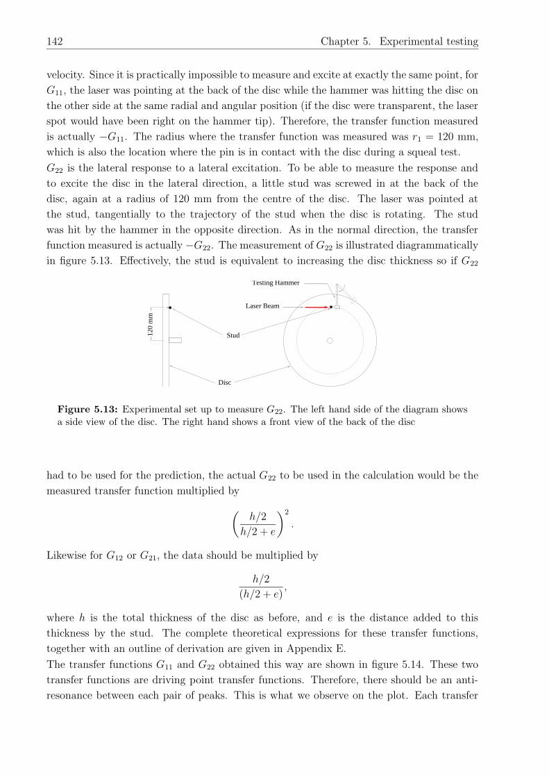
142 Chapter 5. Experimental testing
velocity. Since it is practically impossible to measure and excite at exactly the same point, for
G11, the laser was pointing at the back of the disc while the hammer was hitting the disc on
the other side at the same radial and angular position (if the disc were transparent, the laser
spot would have been right on the hammer tip). Therefore, the transfer function measured
is actually −G11. The radius where the transfer function was measured was r1 = 120 mm,
which is also the location where the pin is in contact with the disc during a squeal test.
G22 is the lateral response to a lateral excitation. To be able to measure the response and
to excite the disc in the lateral direction, a little stud was screwed in at the back of the
disc, again at a radius of 120 mm from the centre of the disc. The laser was pointed at
the stud, tangentially to the trajectory of the stud when the disc is rotating. The stud
was hit by the hammer in the opposite direction. As in the normal direction, the transfer
function measured is actually −G22. The measurement of G22 is illustrated diagrammatically
in figure 5.13. Effectively, the stud is equivalent to increasing the disc thickness so if G22
120
mm
Disc
Stud
Laser Beam
Testing Hammer
Figure 5.13: Experimental set up to measure G22. The left hand side of the diagram showsa side view of the disc. The right hand shows a front view of the back of the disc
had to be used for the prediction, the actual G22 to be used in the calculation would be the
measured transfer function multiplied by
(h/2
h/2 + e
)2
.
Likewise for G12 or G21, the data should be multiplied by
h/2
(h/2 + e),
where h is the total thickness of the disc as before, and e is the distance added to this
thickness by the stud. The complete theoretical expressions for these transfer functions,
together with an outline of derivation are given in Appendix E.
The transfer functions G11 and G22 obtained this way are shown in figure 5.14. These two
transfer functions are driving point transfer functions. Therefore, there should be an anti-
resonance between each pair of peaks. This is what we observe on the plot. Each transfer

5.3. Description of the disc 143
0 2000 4000 6000 8000 10000 12000 14000 16000 18000
−50
−40
−30
−20
−10
0
10
20
30
40
Frequency (Hz)
Tra
nsfe
r fu
nctio
n (d
B)
Figure 5.14: Transfer functions G11 (blue) and G22 (red).
function was obtained by averaging 40 consecutive measurements. The amplitude peak-
trough is around 80 dB, which is the maximum dynamic range which can be measured by
the acquisition card. In spite of some noise, especially around the anti-resonances where the
signal is very small, the peak frequencies are unambiguous. It is also clear that the damping
is very low, especially for the purely diametral modes. A clear peak around 600 Hz is a
good candidate for mode (0,0), although this could also be a strong bending mode of the
shaft. However (0,1) and (0,2), expected around 2400 Hz and 9700 Hz respectively, are still
conspicuously missing from G11 (they are not expected to be visible on G22). A possible
explanation for this absence is that the stud may be located close to a nodal circle.
On the plot of G22, we can clearly see three in-plane modes of the disc within the range
displayed. They can easily be identified because they do not appear in G11 at all. Their
frequencies are at 8750 Hz, 14580 Hz and 16255 Hz. These are plausible values for in-plane
modes: the shear and compressional wave speeds for aluminium are 3.1 × 10³ m/s and
6.15× 10³ m/s respectively. For the lower modes, the wavelength will be of the order of the
diameter 2Ro 0.5 m so that the lowest in-plane mode frequency is expected around 6 kHz.
It is well known that each out-of-plane mode of a disc with at least one nodal diameter is
actually a degenerate pair of modes: there are two different modes that happen to have
exactly the same frequency if the disc is perfectly axisymmetrical. The two modes of any of
these pairs have the same number of nodal diameters and possibly circles, but the pattern is
rotated so that each nodal diameter of one lies on an anti-nodal diameter of the other, thus
ensuring orthogonality.
However, in practice even very slight imperfections prevent most of these doublet modes
from having two strictly identical frequencies. They usually appear as pairs of peaks with
very close frequencies, known as split modes. In our case, the symmetry is reduced by
the stud used to measure the lateral motion. The stud is effectively a small lumped mass.

144 Chapter 5. Experimental testing
The effect of such a perturbation is thoroughly explained in Rayleigh (1894, reprint 1945),
§221: the pair of modes will be split so that the stud lies on a nodal diameter of one of
the modes and on an anti-nodal line of the other one, making the effect of the perturbation
respectively minimum and maximum, in accordance with Rayleigh’s principle. In the former
case, the frequency of the perturbed system will be the same as that of the unperturbed one
(ignoring rotational inertia of the stud). In the latter, the natural frequency will be lower
than the original one (provided the stud is not located on a nodal circle of that particular
mode.) This is in complete agreement with our measured transfer functions. For both G11
and G22, the measurement was made at the stud location, that is on the nodal line of the
higher mode and the anti-nodal diameter of the lower one. Therefore G22 always displays
the higher frequency of the pair, whereas G11 displays the lower one. This reasoning is
illustrated diagrammatically in figure 5.15(a) and this behaviour is shown on the actual data
in figure 5.15(b). When the stud is on an anti-nodal line, it has no lateral motion at all
Laser beam
Node
Anti−node
Stud
(a) Lateral motion of the stud when on ananti-nodal line (top) and on a nodal line
(bottom).
3585 3590 3595 3600 3605 3610 3615 3620 3625
−20
−10
0
10
20
30
40
Frequency (Hz)
Tra
nsfe
r fu
nctio
n (d
B)
(b) Zoom of G11 (top) and G22 (middle)around frequency of mode (4,0).
Figure 5.15: (a) Diagram showing the movement of the stud when the disc vibrates in adiametral mode. (b) Zoom of G11 (top) and G22 (middle) around mode (4,0) at 3600 Hz. Thelower curves are G21 and G12. The two curves are nearly identical and very small. They alsoshow both modes at the same time.
whereas this lateral motion is at a maximum when it is on a nodal diameter.
Figure 5.15(a) also illustrates that, as the testing hammer hits the stud laterally, the lower
mode is probably scarcely excited. Therefore, even if the modes with only nodal circles were
visible on G11, they would not appear on G22 since they involve no lateral motion of the
stud.
Split modes are potentially of interest. Some authors (North (1972) for instance) have

5.3. Description of the disc 145
argued that brake noise results from ‘flutter instability’, and that ‘flutter instability’ means
‘coalescence’ of two eigenvalues of the system when a parameter is varied (bifurcation).
Doublet modes are good candidates for coalescence since their frequencies are already very
close. Mottershead and Chan (1995) claim to show that these are precisely the cause of
noise.
To conclude the description of the vibration of the disc, figure 5.16 shows three transfer
functions G11, G12 and G21. The two bottom curves in figure 5.15(b) are the cross transfer
0 2000 4000 6000 8000 10000 12000 14000 16000 18000
−60
−50
−40
−30
−20
−10
0
10
20
30
40
Frequency (Hz)
Tra
nsfe
r fu
nctio
n (d
B)
Figure 5.16: Transfer functions G11 (top), G12 and G21 (bottom) showing good reciprocityand low level of cross transfer functions.
functions G21 and G12. Top curve (blue) is G11. As expected from reciprocity, the two cross
terms are almost identical. Their very small amplitude levels confirm that the normal and
lateral motions are almost completely uncoupled for the disc, a conclusion reached in chapter
3 from a symmetry argument.
Obtaining a good reciprocity gives good confidence in the measurements. To reach this level
of agreement between the two cross-terms required considerable care in the measurement.
There is infinite scope to point the laser beam at a slight angle to the required direction,
or for the hammer not to hit at the exact point. This sensitivity can be related to the
sensitivity of friction-induced vibration in general. The squeal frequencies predicted by the
theory presented in chapter 3 and 4 are mainly dependent on the dynamical properties of
the subsystems and the coefficient of friction. The capriciousness of friction induced noise
is almost always attributed to the inconsistency of the frictional element (the tribology).
However, repeated measurements on the disc over the duration of this thesis showed that the
mechanical properties of the subsystems can vary substantially too. If one day, a modal test
is carried out on the disc for instance, the next day, most of the frequencies will have shifted

146 Chapter 5. Experimental testing
by about 10 Hz. If the natural frequency of a mode of one subsystem is close to a natural
frequency of the other subsystem, then such frequency shifts could cause a rearrangement in
the clusters of three modes whose importance was highlighted in chapter 3. The difficulty
in obtaining good measurements, which are not contaminated by theoretically unwanted
elements (e.g. the transfer functions of the pin should not contain any torsional mode) points
towards a practical difficulty. With care, it is possible to control the direction of the laser
beam and the location of impact of the hammer. However, during a squeal test, such precise
positioning is much more difficult. The position of the pin subsystem relative to the disc is
only approximate and impossible to repeat to the accuracy necessary to obtain repeatable
measurements for the transfer functions. In the next section, the data collected in this
section and the previous one will be used to test the theory. The problem of deciding which
modes to include in the function D – those that one would expect in a perfect measurement
or those obtained from an approximate positioning? – will be particularly critical.
5.4 Testing of the theory with a constant coefficient of
friction.
The last two sections described how the elements necessary to test the theory presented in
chapter 3 were obtained for the experimental rig under investigation. In order to solve for
the zeros of the function D(ω), it is necessary to process some of the data first.
5.4.1 Fitting of the transfer functions
Provided a vibrating system is linear and its damping is not too large, the theoretical expres-
sion of the transfer function for this system is known to take the form (Skudrzyk (1968)):
Hn(ω) =m∑
k=1
ckn
ω − ωk
+c∗kn
ω + ω∗k
(5.14)
where
ω is the frequency,
ωk = ωk(1 + 2i/Qk),
ωk and Qk are, respectively, the kth natural frequency and the Q factor,
ckn is the residue for the kth mode for transfer function n,∗ denotes complex conjugate,
and m is the number of modes.
Fitting a transfer function means adjusting the values of ωk, Qn and ckn so that the theoretical
curve becomes as close as possible to the experimental one. A successful fitting procedure
provides a mathematical expression for the data.
The main reason for seeking a mathematical expression for the transfer functions obtained
previously is that the zeros of D need to be found in the complex plane. An experimental

5.4. Testing of the theory with a constant coefficient of friction. 147
transfer function is a complex valued function (due to the Fourier transform) of a real valued
variable (the frequency). In order to investigate where the zeros of
D = G11 +H11 + µoH12
lie in the complex plane, it is necessary to know what values D(ω) takes when ω is complex
and not only when it is real. It would not be possible to obtain its (non-real) zeros without
a mathematical expression for the transfer functions. Fitting the transfer functions also
has the incidental advantage of ridding the data of any noise. Once the properties of the
system are gathered in as finite set of parameters, it becomes possible to carry out parameter
studies, such as investigating the effect on the unstable zeros when a given Q factor or natural
frequency is varied. Carried out systematically (i.e. on all the parameters), this study could
reveal which parameters the system is most sensitive to.
The method used for fitting is a global multi-degree-of-freedom algorithm originally imple-
mented for a previous project (Duffour (1998)) and further improved by Adhikari (2000).
The general principles can be found in Ewins (2000),p 331-335 whose presentation is followed
here. Given a set of N experimental transfer functions Yn(ω), and the theoretical expression
Hn given by equation (5.14), the objective is to adjust the parameters of this theoretical
expression so as to minimise in the least square sense the merit function defined by:
χ2 =N∑
n=1
∫
ω∈Ω
|εn(ω)|2dω
=N∑
n=1
∫
ω∈Ω
εn(ω)ε∗n(ω)dω ,
(5.15)
where
εn(ω) = Yn(ω) −Hn(ω).
Hn is a linear function of the residues cnk so that these can be obtained from a simple linear
least-square method. For the Q-factors and the natural frequencies, a non-linear least-square
algorithm is necessary. Following Press et al. (1992), the Levenberg-Marquardt method was
implemented. This is an iterative method shifting gradually from a gradient method far
from the minimum, to a Gauss-Newton method as the minimum is approached. Fitting by
this method has the important advantage of yielding an optimised single natural frequency
and Q-factor for each mode. A successful fitting relies on fairly good initial guesses, which
in our case were obtained by circle fitting on each individual mode and transfer function.
The final result for the fitting of G11 by this method is shown in figure 5.17. This plot
shows that good fitting was eventually obtained as the two curves appear almost super-
imposed. Although fitting is not conceptually a very difficult problem, reaching a good level
of agreement over more than 20 kHz requires overcoming numerous technical difficulties.
The result is only shown for G11 because it was by far the most difficult case, because it
contains many modes, with very different amplitudes and occasionally with moderate overlap.

148 Chapter 5. Experimental testing
0 2000 4000 6000 8000 10000 12000 14000 16000 18000−60
−40
−20
0
20
40
60
Frequency (Hz)
Log
Am
plitu
de d
B
Figure 5.17: Fitting of G11. The solid line is the original data; the dashed line shows itsfitted version.
Equally good fitting could be obtained for the two transfer functions of the pin subsystem.
The Matlab program used for fitting computes complex residues, which is consistent with the
expression used for the transfer function. Therefore, complex modes were available. Most
of the modes of the system were lightly damped, so that real mode shapes are sufficient
for a good fitting. Therefore, only the real part of the residues was kept for the testing.
The fitting was still very satisfactory. Complex amplitudes will be useful in the future to
investigate the effect of non proportional damping on the stability.
Finally, the laser vibrometer provides a measurement of the velocity, but the transfer func-
tions were fitted as the ratio of a displacement over a force, with due account given to the
factor iω. Note that all the measurements were carried out with exactly the same calibra-
tion settings throughout. The transfer functions themselves were not calibrated, because it
is sufficient to know them multiplied by an unknown but common factor.
5.4.2 Computation of the predicted zeros of the coupled system
Fitting the transfer functions G11, H11 and H12 condenses the information contained in the
measurements into two vectors: one for the residues and one for the complex frequencies
ωk = ωk(1 + 2i/Qk). Before using this data for the prediction, the set of frequencies for the
pin subsystems was modified to take into account the lighter mass of the polymer tips used
during a squeal test. This was mentioned in section (5.2.4). The shift is fairly substantial
as Table 5.2 shows. The frequencies obtained from fitting the transfer functions were simply
replaced by the higher values obtained from simple modal test on the cylindrical shell fitted
with a polymer tip. It is possible that this difference in mass also slightly modifies the

5.4. Testing of the theory with a constant coefficient of friction. 149
Steel tip 18.7 940 2834 11710 21810
Polymer tip 18.7 962 2930 12440 22895
Table 5.2: Table showing difference in natural frequency of the pin subsystem (in Hz) whena steel tip and when a polymer tip were fitted. The steel tip was used to measure the transferfunctions up to high frequencies. Polymer tips were used for squeal tests to prevent permanentdamage on the disc.
values of the mode shape coefficients, however these were kept unchanged: if, for a given
pin transfer function, the measurements with the two different tips (steel and polymer)
are plotted together, the peak amplitudes appear hardly affected. In principle, it is also
possible to estimate the effect of the tip mass by modelling it as a point mass at the contact
point. Regarded as two linear systems in series, whose transfer functions are known, the
transfer function for the coupled system (point mass with pin assembly) can be expressed
using standard formulae Ewins (2000). When this was attempted, it was not possible to
match all the frequencies by adjusting the value of the point mass. Furthermore, the shift
in frequencies due to the mass is so large at higher frequencies that the shifted modes move
close to antiresonances. This leads to noisy resonant peaks, from which it is difficult to
extract accurate information.
Since G12 is very small, the disc modal properties influence the prediction solely through G11.
This transfer function was fitted using only one frequency for each doublet mode. The higher
frequency was simply not included in the initial guesses for fitting. The second frequency of
each doublet would be necessary for testing the theory with a varying coefficient of friction,
since then, G22 features in the stability criterion.
For both subsystems, natural frequencies up to 20 kHz were included in the computation of
the zeros. Once the complex frequency and amplitude vectors are known, a Matlab program
computes the coefficients of the polynomial P (ω) defined as the numerator of D(ω) when D
is written as the ratio of two polynomials D(ω) = P (ω)/Q(ω) (c.f. chapter 3, section (3.3)).
The zeros of D(ω) are then found by calling the Matlab routine “roots.m” for P (ω). This
provides a set of complex zeros which can be plotted in the complex plane. To investigate
the influence of the coefficient of friction µ in a systematic way, the zeros were computed
for values of µ ranging from 0.1 to 0.6 incremented by 0.015. From the sign conventions
defined in figure 3.1 and the sign conventions intrinsic to the measuring equipment (e.g. the
laser vibrometer measures positive velocities when the body moves towards the measuring
head), a negative coefficient of friction corresponds to a disc rotating anticlockwise when
viewed from the other side of the motor, whereas a positive µ corresponds to the opposite
direction.

150 Chapter 5. Experimental testing
5.4.3 General description of a squeal test
The phrase “squeal test” refers to the action of applying the pin with a given normal preload,
on the disc spinning at a given rotation speed and measuring the quantities described next
when a squeal occurs. Before the results were permanently recorded, a test was usually
repeated a few times with the same parameter values to try and identify the typical be-
haviour of the rig on that day, with those settings. Usually, repeatability within 5 or 10
minutes, without modifying the mechanical set-up (for instance unscrewing a bolt) was not
too difficult.
Before starting the actual test, the gauges were calibrated, following the procedure described
in section (5.2.2). As explained, accurate calibration factors are essential for a good deter-
mination of the coefficient of friction. As the calibration factors showed some variation from
one day to the next, it was necessary to carry out a complete calibration at least once a day.
Once calibrated, the bridges were accurately balanced if this was necessary (this was usually
the case). Then the pin was clamped in position such that the tip of the pin was in contact
with the disc at the exact radius where the measuring stud on the disc was located (i.e. at
the radius where the transfer functions for the disc were measured).
Two input parameters could be controlled. (1) The normal preload of the pin on the disc:
this could be read on an oscilloscope from the appropriate set of strain gauges fitted on the
cylindrical shell of the pin. (2) The rotation speed of the disc. The disc was driven by a DC
electric motor of nominal output speed 1500 r.p.m. This speed was reduced by a gear box
fitted on the output shaft of the motor. The gear reduction ratio is 75. The output speed
of the two coupled together could be varied from 0 to a few tens of rotations per minute,
using an electric controller. The rotating speed of the disc could be monitored during a run,
reading or logging the output of a tachometric sensor fitted on the shaft driving the disc.
Three output parameters were recorded: the normal and friction force at the contact point
were measured from the strain gauges as explained in the section describing the top hat
cylinder. The noise was recorded using a standard microphone located near the contact
point. In all, four signals were recorded during a run:
The rotation speed of the disc from the tachometer signal.
The friction and normal forces from the strain gauges.
The acoustic signal from the microphone.
The maximum sampling rate of the data acquisition card was 200 kHz. Used at its maximum,
each signal was logged at 50 kHz.
Once recorded, the microphone signal time history was processed into a sonogram. A sono-
gram has the advantage over a standard spectrum that it provides a good indication of the
time at/during which a given noise occurs (as well as its frequency).
Tips made of two materials were used: Nylon and Perspex. Perspex was used more often
because it gives a higher coefficient of friction, which led to a richer array of behaviours. The
tips all had similar shapes: a screw with a hemispherical head. Each was machined out of a
single piece of material. Several were needed as they tend to wear fairly quickly (especially

5.4. Testing of the theory with a constant coefficient of friction. 151
Perspex). Tips were used for squeal test until the contacting region was worn to a disc of
approximately 3 mm in diameter.
The rig has a peculiarity which it was not thought necessary to correct as it proved useful:
misalignments of the disc with the main axis of the motor caused a substantial out-of-plane
displacement of the disc of a few tenths of a millimeter. In practice, this means that when
the pin is clamped in contact, the normal load varies as the disc rotates.
The disc has another peculiarity: hitting its surface with the testing hammer resulted in
small impact marks at the exact location where the tip of the pin would later pass. To
prevent gross irregularities in the surface, the zone with hammer impacts was gently rubbed
with some fine sandpaper. This removed the impact traces but left a patch with a surface
finish much coarser than anywhere else on the disc. When the tip of the pin runs through
this patch, the coefficient of friction increases appreciably.
5.4.4 Comparison of the computed unstable zeros with the mea-sured squeal frequencies
Experiments in friction-induced vibration are extremely difficult because they usually present
very poor repeatability, even under apparently identical external conditions. The behaviour
of the rig presented in this chapter is no exception to this rule. This makes the task of
testing a theory particularly delicate. The formalism presented in chapter 3 yields definite
predictions of unstable frequencies. How are these to be compared with sporadic occurrences
of various noise frequencies?
To investigate in a somewhat systematic way the behaviours the rig could exhibit, similar
squeal tests were carried out every day over a week. Although a large amount of data has
be collected at the various stages of the rig, this chapter mainly analyses the data collected
over this sequence of measurements. The transfer function matrices were measured twice:
once before starting any squeal test and once at the end of the week of measurement. The
transfer functions shown so far in this chapter are taken from this second and final set of
measurements. It will appear that there are good reasons to measure the transfer function as
often as possible. In principle, it may even be desirable to measure them before every squeal
test. However, obtaining good measurements of the transfer functions itself requires a whole
day. Identifying the range of behaviours that the rig can exhibit for a given configuration
(i.e. once the pin assembly is clamped into position for a test) also takes time.
The initial prediction
First, the set of zeros predicted from the initial measurement of the transfer functions is
described. Figure 5.18 shows the predicted zeros of the function D in the complex plane.
Figure 5.18(a) corresponds to an anticlockwise rotation of the disc as viewed from the pin
(µ < 0), while figure 5.18(b) shows the zeros when the disc rotates clockwise. These two
plots show the zeros as dots going from blue to red as the coefficient of friction increases
from 0.1 to 0.6 by increments of 0.015. On the horizontal axis, the natural frequencies of the

152 Chapter 5. Experimental testing
0 2000 4000 6000 8000 1000012000140001600018000−500
−400
−300
−200
−100
0
100
200
300
400
500
Real part of the roots (Hz)
Imag
inar
y pa
rt o
f the
roo
ts
(a) µ < 0.
0 2000 4000 6000 8000 1000012000140001600018000−500
−400
−300
−200
−100
0
100
200
300
400
500
Real part of the roots (Hz)
Imag
inar
y pa
rt o
f the
roo
ts(b) µ > 0.
Figure 5.18: Plots showing the predicted zeros of the coupled system when the disc rotatesin two opposite directions. (a) When the rotation is anticlockwise , as viewed from the pin(µ < 0), one unstable zero is predicted at around 12 700 Hz. (b) When the disc rotatesclockwise (i.e. µ > 0), a different zero is predicted to be unstable at 3 225 Hz.
(uncoupled) pin subsystem are shown as green circles (), while those of the disc are shown
as green plus signs (+). The vertical scale of the plot has been limited to allow a clearer
display of the important features. Some extra zeros with large positive imaginary parts are
not shown.
When the disc rotates anticlockwise (i.e. for µ < 0), only one zero is predicted to be unstable
at 12 700 Hz for the range of values of the coefficient of friction. From the plot shown in
figure 5.18(a), this zero becomes unstable when the coefficient of friction becomes greater
than 0.49 (in absolute value). However, shifting slightly the 12 460 Hz pin mode frequency
can significantly alter this threshold: if this pin mode frequency is set to 12 450 Hz, the
threshold is µ = 0.565, whereas if the frequency is set to 12 490 Hz, the zero becomes
unstable for µ = 0.44. If the value of the coefficient of friction is allowed to reach 0.7, a
second unstable zero becomes unstable around 850 Hz.
When the disc rotates in the clockwise direction (i.e. µ > 0), again a single zero is predicted
to be unstable. Its frequency is around 3200 Hz and it crosses the stability threshold when
µ = 0.46. This time, shifting slightly the nearest pin mode frequency (at 2930 Hz) does
not have such a strong effect on the threshold of stability, possibly because there is no disc
mode in the close vicinity of this frequency. Note that as µ increases, the imaginary part
of the unstable zero goes down to around -1500. Only the zeros down to -500 are shown.
Qualitatively, these predictions support very well the theory presented chapter 3. The modal
density of the disc is much higher than that of the pin; therefore, wherever there is a pin

5.4. Testing of the theory with a constant coefficient of friction. 153
mode, it is bound to be surrounded by two disc modes. If the corresponding composite
modal amplitude “ai” for this pin mode is negative (which is more likely for larger values
of the coefficient of friction), then a cluster of three modes with “composite amplitudes” of
alternating signs is formed. Therefore, the unstable zeros are more likely to appear near the
pin modes, which is what is observed here: the three possible unstable zeros correspond to
the frequencies: 850 Hz, 3200 Hz and 12 700 Hz. These are all close to the pin subsystem
natural frequencies: 960 Hz, 2 930 Hz and 12 460 Hz.
Description of some results from the squeal tests
The sequence of squeal tests described next was carried out as follows. A test can essentially
be identified by the disc average rotation speed. A set of three speeds was chosen: 3, 7 and 15
r.p.m. Each angular velocity can be either clockwise or anticlockwise so that a complete set
of measurements comprises 6 squeal tests: the three values above for each direction. When
the pin was first preloaded on the disc at rest then the motor set to the required value, the
pin usually went through a stick-slip regime at very low speeds. Since the theory predicts
the stability of the steady sliding regime, starting with a complex non-linear vibration was
undesirable for testing purposes. To avoid this problem, the disc was first set to the required
rotation speed, then the pin was pushed onto the disc using the preloading spring. This
succeeded in stopping the initial occurrence of stick-slip, therefore this way of starting a test
was always used.
The results from three tests will now be described in detail. These tests were carried out
using Perspex tips. The first was carried out early in the week. The rotation was clockwise
at 6.8 rpm. Figure 5.19 gathers the data obtained in three plots.
At the top, the signal from the microphone is shown in the form of a sonogram. The middle
plot shows time histories of the normal (bottom, green) and friction (top, blue) forces, once
calibrated. The third, bottom plot shows the time history of the coefficient of friction. These
three plots are aligned so that the horizontal axis, showing the time is the same for all of
them. This allows the precise location in time of an event. For example, a burst of noise
between 1.4 and 1.5 s is visible on the three plots. As mentioned in the description of the
cylindrical shell (section (5.2.2)), the force signal are fairly noisy. This noise is also visible
in the coefficient of friction. The sign of the forces is arbitrary: it is a result of the way the
gauges have been wired. As the rig stands, the friction force should be positive when the
disc rotates anticlockwise. The slow variation in the normal force is due to the macroscopic
deflection of the disc described as a peculiarity of this rig in the previous section. The friction
force increases accordingly so that the coefficient remains fairly constant at an average of
0.52. This value is fairly high, but it is typical of the values of µ measured with Perspex on
Aluminium.
The sonogram shows a main squeal frequency at 2 670 Hz. It first appears sporadically
before 1.5 s, then remains sustained. A second squeal frequency, much fainter, appears at
5 435 Hz. There is also a short contour at 12 500 Hz around 0.5 s. During the time intervals

154 Chapter 5. Experimental testing
0 0.5 1 1.5 20
0.5
1
1.5
2x 10
4
Fre
quen
cy (
Hz)
0 0.5 1 1.5 2−40
−20
0
20
For
ces
(N)
0 0.5 1 1.5 20
0.5
1
Time (s)
µo
Figure 5.19: Set of three plots showing a sonogram of the microphone signal (top), thetime history of the calibrated normal (green) and friction (blue) forces (middle); and the timehistory of the coefficient of friction).
when these frequencies appear on the sonogram, the force time histories show distinctively
larger amplitudes. Although the coefficient of friction remains broadly constant, stronger
oscillation also shows in its time history during those spells. This suggests that Coulomb’s
law may not be quite valid at higher frequencies. It might also be due to a calibration effect.
Showing a single case is not intended to prove that the theory is valid or not. At this stage,
the objective is simply to give general comments on the measurements obtained. However,
it is remarkable that the first and strongest frequency, which appears at 2 670 Hz, is fairly
close to the predicted 3.2 kHz. There is also a persistent squeal frequency at 21 kHz which
occurs very often when the disc rotates clockwise. This squeal frequency was not predicted.
This might be due to the quality of the transfer function measurements which significantly
deteriorates after 20 kHz. Predicting this frequency would also probably require higher
modes to be taken into account. Whatever the reason is, 21 kHz is well above the audible
range, which is our primary concern.
For each test, the signals were recorded for 5 s. This is also true of the data shown in
figure 5.19. The plots only show the data up to 2.5 s because after that time, the noise

5.4. Testing of the theory with a constant coefficient of friction. 155
evolved into a very loud noise, where losses of contact occurred. The regime is then highly
non-linear so that the theory presented in this thesis is not expected to be valid. The
non-linear behaviour nevertheless presents some interest. An example will be described in
the next section. This non-linear regime is not specific to this test. It occurs particularly
frequently at the lower values of the disc speed (3 and 7 rpm).
To conclude on this test, it is noteworthy that the biggest vibration visible in the force time
histories occurs when the normal force reaches its maximum (here about 20 N). This is a
very common observation: the variation of the mean normal load does not seem to affect
significantly the squeal frequencies, but it does appear to have a triggering effect. Below a
minimum value of N , the rig can be silent. This value can be very low especially at low
disc speeds; then the rig squeals as soon the pin is in contact. While the rig is squealing,
increasing the normal load often causes the squeal to evolve into the highly non-linear regime
mentioned above. Again, this is more frequent at low disc speeds.
The second test described was carried out at the beginning of the week. The rotation speed
was also the same, 7 rpm, but the direction was anticlockwise. Figure 5.20 shows the data
from another test under the same format. The force time histories show that little occurs
0 0.1 0.2 0.3 0.4 0.5 0.6 0.7 0.8 0.9 10
0.5
1
1.5
2x 10
4
Fre
quen
cy (
Hz)
0 0.1 0.2 0.3 0.4 0.5 0.6 0.7 0.8 0.9 1−40
−20
0
20
For
ces
(N)
0 0.1 0.2 0.3 0.4 0.5 0.6 0.7 0.8 0.9 1−4
−2
0
2
Time (s)
µo
Figure 5.20: Set of three plots showing a sonogram of the microphone signal (top), thetime history of the calibrated normal (green) and friction (blue) forces (middle); and the timehistory of the coefficient of friction).

156 Chapter 5. Experimental testing
before t = 0.9 s. Then, both forces display strong oscillation. The plot stops at this point
as it can be seen that the friction force reaches positive values. This indicates that the pin
is slipping forward. In mathematical terms, the regime is piece-wise linear, therefore non-
linear. Therefore only the incipient stage of the noise is shown, where the theory is expected
to be valid.
The sonogram reveals several different things:
A fuzzy frequency band decreasing from 17.5 kHz to 16.5 kHz as time increases. The
dark colors of the contours indicate that this drifting frequency has a fairly low amplitude.
A faint and intermittent frequency band at 940 Hz, running for the whole duration shown.
A frequency at 12 470 Hz starting at around 0.45 s and increasing in amplitude as time
increases.
A ridge at 15 275 Hz, starting much later.
For times later than those displayed, the noise settles into a very strong oscillation at 12.5 kHz
during which the friction continues to oscillate in sign.
During the times displayed, the average coefficient of friction was measured at 0.7. This
is surprisingly high. It is possible that one of the bridges has drifted significantly out of
balance. This often occurs for the normal force, but hardly ever for the friction force so that
it is very unlikely that the change in sign observed in the friction force might be due to a
bridge unbalance.
Comparing this set of squeal frequencies with the predictions shown in figure 5.22, it tran-
spires that the 12.47 kHz as well as the ridge at 940 Hz were very well predicted. The 12 kHz
noise is of particular interest as it represents the incipient stage of a subsequent strong insta-
bility. As noticed before, the noise at 17 kHz is outside the audio range. The drift it displays
might be correlated with the variation of the normal force. If this is the case, this is clearly
reminiscent of the results obtained in chapter 4, when the coefficient of friction is allowed to
vary with the sliding speed, for then the normal load features in the stability criterion. This
may explain why it was not predicted. This may also be true of the non-predicted 15 kHz
frequency. As this frequency arises much later, it is also possible that it is a harmonic or
resulting from the system drifting into non linearity. This completes the description of this
test.
The last test described was carried out on the last day. The rotation speed was 15 rpm
clockwise. The results are shown in figure 5.21 using the same format as before. The rig
was fairly quiet although the microphone recorded strong oscillation at 25 kHz, which is
well outside the range of interest. The force time histories show two interesting features. At
t ∼ 0.5 s and t ∼ 4.5 s, the friction force shows a strong short variation. This corresponds
to the passage of the tip through the rough patch resulting from the sand paper polish.
At 15 rpm., the disc speed is large enough so that two passages could be recorded within
a time sample of 5 s. This generated a short burst of noise whose frequency content is
revealed by the sonogram: 2800 Hz and 5500 Hz. Throughout the time sample, a faint
discontinuous line appears on the sonogram at 6400 Hz. When the normal force is maximum,
between 1 and 1.5 s, a noise reappeared with a similar frequency content. This confirms the

5.4. Testing of the theory with a constant coefficient of friction. 157
0 0.5 1 1.5 2 2.5 3 3.5 4 4.50
0.5
1
1.5
2x 10
4F
requ
ency
(H
z)
0 0.5 1 1.5 2 2.5 3 3.5 4 4.5−100
−50
0
50
For
ces
(N)
0 0.5 1 1.5 2 2.5 3 3.5 4 4.5−5
0
5
10
Time (s)
µo
Figure 5.21: Set of three plots showing a sonogram of the microphone signal (top), thetime history of the calibrated normal (green) and friction (blue) forces (middle); and the timehistory of the coefficient of friction).
triggering effect of the normal load. The normal force time history shows occasional drops
in magnitude. The reason for these is unknown but a close examination of the time history
suggests that it may be due to electrical interference rather than a mechanical effect. These
drops cause the coefficient of friction to jump correspondingly. Noise in the coefficient of
friction also increases as the normal force becomes close to zero. As the mean normal preload
decreases in amplitude, the effect of the noise on the coefficient becomes more significant.
Overall, the value of the coefficient of friction remains constant.
µ = 0.5 is the typical value for Perspex on Aluminium. If the rig is left running for a
long time with the same tip in the same position, it is possible that the tip wears so that
the contact becomes more conforming. This could increase the true area of contact and
thus increase the coefficient of friction. Such a situation was observed. The rig was then
highly unstable: the regime would be non-linear as soon as the pin was loaded in contact.
Inspecting the tip afterward, it appeared that the contact layer had melted during the test.

158 Chapter 5. Experimental testing
The geometry of the contact zone was then highly irregular. All the results shown so far were
carried out using a perspex tip. As mentioned before, tests were also carried using nylon
tips. The coefficient of friction between Nylon and Aluminium was consistently measured
at 0.15. For this value the theory does not predict any squeal and no squeal was observed
if only a faint 12500 Hz, after letting the disc running for a long time. The next section
presents the predicted zeros based on the transfer functions measured at the end of the week
of testing.
The final prediction
The results are shown in figure 5.22 for negative (a) and positive (b) coefficients of friction.
As before, these two plots show the zeros as dots going from blue to red as the coefficient
0 2000 4000 6000 8000 10000 12000 14000 16000 18000−500
−400
−300
−200
−100
0
100
200
300
400
500
Real part of the roots (Hz)
Imag
inar
y pa
rt o
f the
roo
ts
(a) µ < 0.
0 2000 4000 6000 8000 10000 12000 14000 16000 18000−500
−400
−300
−200
−100
0
100
200
300
400
500
Real part of the roots (Hz)
Imag
inar
y pa
rt o
f the
roo
ts
(b) µ > 0.
Figure 5.22: Final prediction of the zeros plotted in the complex plane.
of friction increases from 0.1 to 0.6. On the horizontal axis, the natural frequencies of the
(uncoupled) pin subsystem are shown as green circles (), while those of the disc are shown
as dark green plus signs (+).
Overall, the prediction is recognizably similar to the initial one. However, there are significant
changes in the detail. For negative coefficient of friction (disc anticlockwise), the single
unstable zero at 12500 Hz has become a cluster of three unstable zeros. Their frequencies
are approximately: 11500, 12000 and 12500 Hz. As before, allowing the coefficient of friction
to reach sightly higher values (0.7), the next zero to become unstable is at 850 Hz. When
the disc rotates clockwise, the prediction is much more similar to the initial one: the only
single zero predicted to be unstable is at 3300 Hz. In the initial prediction, increasing the
coefficient of friction up to high values (µ = 1) did not cause any new zero to become
unstable. This time, a zero at 4900 Hz crosses the stability threshold when µ = 0.75. This
is clearly reminiscent of the new 5500 Hz squeal frequency observed in the last test. Similarly
in the clockwise direction, it is remarkable that new frequencies are predicted slightly lower

5.4. Testing of the theory with a constant coefficient of friction. 159
than 12500 Hz when a new squeal frequency is observed at 10000 Hz.
If a colloquial phrase was to describe the general impression produced by comparing the
two theoretical predictions it could be: “almost the same, but not quite”. This would also
describe very well the impression produced by the comparing the final measurements of the
transfer functions with the initial ones. If the fitted results from the initial measurements
were plotted on the same graph as the final measurements, it would be immediately clear
that the overall shape is very similar, but also that some modes need some adjustment in
damping, natural frequency and amplitude. The general impression can also describe the
behaviour observed during the week of experimental testing.
Overall assessment
So far particular examples of squeal tests have been described. For testing purposes, it is
useful to present all the results obtained during the week in a single chart. This was done
in table 5.3. This table gives the main squeal frequencies in Hertz for a given day at a given
Disc speed Prediction 1 Day 1 Day 2 Day 3 Day 4 Day 5 Prediction 2
3 rpm 850 12700 940 + 15 300 940 940 940 940+12500 850 11500/12500
7 rpm 850 12700 12500+15250 12500 12500 12500 12500 850 11500/12500
Anticl
ock
w.
15 rpm 850 12700 12500 12500 12500 12500 10000 850 11500/12500
3 rpm 3200 15250 12500 2750+12500 2600+12500 2800+10000 3300 4900/5500
7 rpm 3200 12500+15250 2700 12500 2700+12500 2800+5500 3300 4900/5500
Clo
ckw
ise
15 rpm 3200 2800+12500 2700 2700+5500 2700+5500 2750+5500 3300 4900/5500
Table 5.3: Table showing the squeal frequencies (in Hz), measured from noise tests on differentdays for different disc speeds. The test numbers, in the first row, are in chronological order.The predicted unstable frequencies have been added in an initial and final column. Theexperimental frequencies printed with a bold (blue) font are the observed noise frequenciesclose to a predicted ones.
speed (in rpm). The tests are given in chronological order so that the test labelled no 1
was done first, etc. The frequencies printed in bold are the experimental squeal frequencies
for which there is a nearby theoretically predicted unstable zero. Frequencies have been
printed in bold even if the prediction is approximate. Thus, the experimentally observed
2700 Hz noise has been considered as a realisation of the 3200 Hz predicted squeal frequency.
The same rule applies for the predicted 4900 Hz and the measured 5500 Hz. Only audible
frequencies were included in the table. In many cases, a squeal frequency at 18000 Hz similar
to that described in the second example was present. They do not appear.
In order to investigate the influence of the exact location of the pin subsystem in the rig,
Tests 2, 3 and 4 were carried out without dismantling the pin. This means that the forces
could not be calibrated for these three tests, so that only estimations based on previous

160 Chapter 5. Experimental testing
calibration factors could be available for the forces. To mark the distinctive feature for these
three tests, their test number has been printed in green. With this piece of information in
mind, it is useful to compare the set of frequencies with each other. First comparing tests
2, 3 and 4 together, it appears that, for given disc speed, their squeal frequencies are very
similar. In the anticlockwise direction, they are completely identical. Comparing this subset
of tests with the initial and the final one, more discrepancies arise. This suggests that the
exact position of the system has a significant influence on the prediction. Uncoupling the
pin assembly and repositioning it causes new frequencies to appear (for instance the 15 kHz
squeal in the anticlockwise direction). The effect due to dismantling cannot be distinguished
from the slight variations the rig undergoes on its own.
The previous subsection described a slight but important variation in the modal properties
of the rig subsystems. This evolution might in part be due to the mounting/unmounting
process. However, the appearance of the new 5500 Hz squeal at 15 rpm clockwise in tests 3,
4 and 5 suggests that the system properties evolve even if no apparent changes are made to
it.
The velocity appears to have a significant effect. First, different frequencies can appear
for different speeds on a given day. Some may be predicted, some may not. Qualitatively,
it appears that the velocity has an influence of which frequency is being “picked” to be
unstable. For instance, at 3 rpm anticlockwise, the 940 Hz squeal is predominant, whereas
at 7 or 15 rpm, 12500 Hz is. The theory presented in chapter 3 cannot account for any
velocity effect. However, the theory presented in chapter 4, with a coefficient of friction
linearly varying with sliding speed, it might be possible to predict these changes. The role
of the normal load previously described supports this suggestion.
The objective of this experiment was to test whether the unstable frequencies predicted by
the simplest realistic theory were experimentally observed. The conclusion from this study
is that to a great extent (75%), the squeal frequencies observed could be predicted by the
simplest linear theory. This does not mean that other effects might not be at play. The
results just shown suggest that a varying coefficient of friction might be such a plausible
effect.
To complete this chapter, an example of non-linear behaviour will now be described. Fig-
ure 5.23 shows some measurements from a run where the disc was rotated clockwise at 15 rpm.
Figure 5.23(a) shows a sonogram of the microphone signal and figure 5.23(b) shows a small
sample of the normal force time history. The sonogram clearly shows the transition from a
linear squeal at the predicted 2700 and 5500 Hz, to a highly nonlinear regime as indicated
by plot (b). The normal force time history shows that losses of contact occur as the normal
force goes to zero during each cycle. In this regime, the whole pin assembly was bouncing on
the disc. The noise corresponding to this nonlinear regime was extremely loud, but without
inspecting the normal force time history, it would not have been possible to identify whether
the regime was linear or nonlinear. This indicates that one should be cautious in trying to
identify a regime from a purely acoustic signal. The sonogram shows that the initial ridge
at 2700 Hz undergoes a sharp transition to a lower frequency at 2100 Hz. This transition

5.4. Testing of the theory with a constant coefficient of friction. 161
0 1000 2000 3000 4000 5000 6000 7000 8000 90000
0.1
0.2
0.3
0.4
0.5
0.6
0.7
0.8
0.9
Frequency (Hz)
Tim
e (
s)
(a) Sonogram of microphone signal.
0.8285 0.829 0.8295 0.83 0.8305 0.831
−70
−60
−50
−40
−30
−20
−10
0
Time in seconds
Nom
al F
orce
(N
)
(b) Normal force time history.
Figure 5.23:
could be heard clearly. Once the system settles into this bouncing mode, a clear set of new
unstable frequencies emerges in the sonogram. Most of these frequencies are close to disc
mode frequencies. It is possible that in this regime, the noise is simply the result of repeated
impacts on the disc. The transition just described is also reminiscent of the concept of mode
locking described in chapter 3: an initially unstable frequency shifts slightly to “locks” into
a close mode of the disc. This is plausible. However, it should be emphasised that this
type of locking probably bears little relation to the type of frequency mergings predicted by
linear theory and described in chapter 3, for instance in figure 3.13. This example puts the
work carried out in this dissertation into perspective since, however well a linear approach
could predict the initial instability, it will give no or very little information on the type of
nonlinear behaviour just shown.

162 Chapter 5. Experimental testing

Chapter 6
Further work and conclusions
Before summarising the main findings of this dissertation, some directions for further research
are suggested.
6.1 Further analytical work
6.1.1 Extension to two contact points
The theory presented in chapter 3 and 4 can be extended so that the two subsystems are in
contact at two points. A diagram of such a system is shown in figure 6.1: With the notation
1 2
Dis
c R
otat
ion
"Brake""Disc"
Fb
a
N
F
a
Nb
u
u
2b
bN
aN
1au
1bu
2a
Fb
a
v
1av
1bv
2b
vF 2a
Figure 6.1: Diagram showing two linear systems in sliding contact at two points. The uppercontact point is labelled “a”, and the lower contact point is labelled “b”. The displacementsare considered at the contact points but are shown shifted apart for clarity.
defined in the figure, the displacements of each system can be related to the normal and
163

164 Chapter 6. Further work and conclusions
tangential forces via matrices of transfer functions defined by
u1a
v1a
u1b
v1b
=
G11(ω) G12(ω) G13(ω) G14(ω)G21(ω) G22(ω) G23(ω) G24(ω)G31(ω) G32(ω) G33(ω) G34(ω)G41(ω) G42(ω) G43(ω) G44(ω)
N ′a
F ′a
N ′b
F ′b
(6.1)
and
u2a
v2a
u2b
v2b
=
H11(ω) H12(ω) H13(ω) H14(ω)H21(ω) H22(ω) H23(ω) H24(ω)H31(ω) H32(ω) H33(ω) H34(ω)H41(ω) H42(ω) H43(ω) H44(ω)
N ′a
F ′a
N ′b
F ′b
(6.2)
Introducing two input roughness parameters ra and rb, such that u2a = ra − u1a and u2b =
rb − u1b, and using the simplest Coulomb’s law with the same or different coefficients of
friction, a criterion for instability can be derived. With a single coefficient of friction, the
criterion is as follows:
This system can be unstable if and only if the function
D(ω) = [G11 + µG12 +H11 + µH12] [G33 + µG34 +H33 + µH34]
− [G31 + µG32 +H31 + µH32] [G13 + µG14 +H13 + µH14](6.3)
has at least one zero in the lower Fourier half-plane.
Following the method used in chapter 3 and 4, the stability of this system can be studied by
simulating the behaviour of generic systems. Of particular interest is the potential occurrence
of modes such that the “brake” rocks from one point of contact to the other. This type of
mode would be truly specific to multiple contact points and would complete the survey of
possible linear routes to instability started in this dissertation. The preliminary study of
the linear stability of a rigid block sliding on a rough plane would be an interesting and
useful case study. Such a system could also serve for a preliminary experimental validation.
In principle, any finite number of contact points could be cast into formulations similar to
equation (6.3). However in practice, the algebra might quickly become unwieldy.
6.1.2 Modelling of the pin top-hat
The rig provides measurements of the friction and normal forces. It was shown in chapter 5
that Coulomb’s law was a good approximation for our system for low frequencies: although
the mean value of the two forces showed significant variations, the coefficient of friction
was on average remarkably constant. However, when strong oscillations due to squeal were
present in the forces, these also appeared in the coefficient of friction. This suggests that a
more complicated friction law my be necessary to describe appropriately the behaviour of
the system at high frequencies. To investigate further the relationship between F and N at

6.2. Further experimental work 165
those frequencies, it is first necessary to verify that the shell embedded in the top hat cylinder
does not possess resonances within the frequency range of interest (roughly below 20 kHz).
Analytical estimation of the first compressive mode is not difficult and an estimate was given
in the description of the pin. Estimating the lower mode corresponding to a shell deforming
in shear or bending is much more difficult. To obtain an estimate for these frequencies, a
finite element modelling of the top hat piece would be useful.
6.2 Further experimental work
6.2.1 Improvements on the existing rig
Validation of the varying coefficient of friction theory
In order to validate the theory presented in chapter 4, where the coefficient of friction is
allowed to vary with the sliding speed, it is necessary to instrument the rig so that the
sliding velocity between the two subsystems can be measured. The tangential velocity of the
tip of the pin could be measured by pointing downward a single point laser vibrometer. The
disc speed could be estimated by improving the current tachometre arrangement. However,
a more accurate measurement of the disc velocity at the contact point might be necessary
to obtain a good measurement of the sliding velocity.
Controlling the experiment by computer
With most (if not all) experimental rigs in friction-induced vibration, it is very difficult to
obtain repeatable and consistent results from friction-induced vibration experiments. As
mentioned in chapter 5, this makes testing any theory particularly difficult. However, the
results presented in Chapter 5 also show that within short time length, and provided the
mechanical set is not disturbed, it is possible to obtain repeatable results. More squeal test
carried out during a single day would be very helpful to survey all the possible behaviours that
a rig can exhibit. To achieve this, a way of operating the rig automatically must be devised.
This involves: (1) driving automatically the disc rotation using a micro-controller card, (2)
controlling the normal preload, (3) detecting the occurrence of noise using a microphone,
the signal from which would automatically trigger the data acquisition system. The relevant
signal would be the friction and normal forces measured by the strain gauges on the thin shell
and possibly the microphone signal and possibly an estimation of the contact temperature.
The sliding velocity, if it can be measured properly, would also be a valuable source of
information. Once this is done, it may become possible to map a set of squeal regimes to
a given set of operating conditions. This data will enormously valuable. If a characteristic
finite set of regimes can be mapped to a set of operating conditions, this will provide a
very useful pool of data to test any theory. The well-known ”capriciousness” of the friction-
induced vibration would be partly overcome. If such a set proves not to manifest itself then
this data would also provide some very interesting information on the phenomenon: the

166 Chapter 6. Further work and conclusions
noise would then be governed by a parameter which is not controlled. If the most obvious
parameters are already carefully controlled, the choice for new ones is greatly narrowed down.
6.3 Conclusions
The primary aim of this research has been to investigate the linear routes to instability
when two subsystems are coupled together by dry friction through a single point contact.
This type of modelling can be regarded as a first step towards a better understanding of the
mechanism(s) underlying brake noise.
The study of a simple model with 2 or 3 degrees of freedoms illustrated the shortcomings
of lumped-parameter approaches commonly used to investigate brake noise. Such models
can be misleading as the predicted stability regions are strongly dependent on the modes
included in the model. Two plausible lumped-parameter models of a pin-on-disc system were
shown to give completely different stability results.
A new approach has been developed, capturing the dynamics of the two subsystems in
contact through appropriate matrices of transfer functions defined at the contact point.
Defining the dynamics in terms of transfer functions eliminates the difficulty of choosing
the relevant modes. For this class of systems, all the conceivable routes to instability were
investigated analytically.
Modelling friction at the contact point with a constant coefficient of friction, a criterion
for stability was derived in terms of the transfer functions. Simulating the behaviour of
generic systems, it was shown that the stability of the coupled system can be understood to
a great extent by considering sequences of three modes of the uncoupled subsystems with
consecutive frequencies. It was demonstrated that instability is more likely to occur if these
modes generate displacements at the contact point with the appropriate pattern of signs.
Numerical simulations on generic systems confirmed that structural viscous damping has a
non-systematic influence on the stability. The study of the influence of damping also revealed
the importance of the spatial distribution of damping in the system.
The influence of a compliant contact was also investigated by introducing linear springs at the
contact point between the two subsystems. Simulated cases showed that contact compliance
had a significant influence on the stability if the stiffness of the contact springs was below
or of the same order of magnitude as the bulk structural stiffness of the system.
Allowing the damping to be non-proportional was proved to result in the system evolving
as a purely real exponential growth or decay according to the amplitude and signs of other
parameters.
A final route to instability was investigated by allowing the coefficient friction to vary linearly
with the sliding speed. This was demonstrated to influence the stability significantly. A
dimensionless quantity was found, featuring average properties of the system. Comparing
the magnitude of this quantity with unity indicates when a varying coefficient of friction has
a significant effect.

6.3. Conclusions 167
A rig was designed in order to test the theory using a constant coefficient of friction. De-
spite the inherent difficulties in obtaining repeatable results, the unstable frequencies were
predicted in 75 % of the cases. Therefore, the simplest linear theory definitely has a pre-
dictive power, provided linear predictions are compared with experimental results obtained
in a linear regime. This conclusion legitimises a posteriori its use to model friction-induced
vibration. It was also shown that other effects were present and caused non-predicted in-
stability. Before introducing any non-linear feature to attempt to account for them, it is
necessary to ensure that these frequencies cannot be predicted by the other linear routes to
instability surveyed in this dissertation.

168 Chapter 6. Further work and conclusions

Appendix A
Proof of the claim made in chapter 3about the zeros of D
This appendix gives a sketch of proof for the claim made in Chapter 3, section 3.3. It was
stated that the D(ω) cannot have zeros in the lower half complex plane, if all the coefficients
ai are positive. To prove this, Nyquist’s criterion is used in conjunction with sign arguments
to show that the image path D(Γ) cannot cross the negative part of the real axis, and
therefore cannot encircle the origin. Γ consists of two parts: the real axis segment [−R R]
and the semi-circular arc of radius R and centred on the origin. These two parts have to be
dealt with separately.
(1) Suppose ω ∈ [−R R]. Consider one of the resonant terms in the expansion 3.13. The
imaginary part of such a term is
−2anωnδnω
(ω2n − ω2)2 + 4ω2
nδ2nω
2. (1.1)
It is clear that expression 1.1 is positive when ω < 0, negative for ω > 0, and that it can only
be zero when ω = 0. At this point, the real part is an/ω2n > 0. Since the ai are all positive,
adding up several resonant terms makes the description just given for one resonant term also
valid for D(ω): for real ω, the imaginary part of D(ω) can only be zero when ω = 0. Then
the real part of D(ω) is∑an/ω
2n, which is a positive number.
(2) Suppose ω = Re−iθ, for θ = 0 to π. For large values of R and most values of θ, a typical
resonant term in expansion 3.13 will be approximately equal to
− an
R2e2iθ.
169

170 Appendix A. Proof of the claim made in chapter 3 about the zeros of D
As θ varies between 0 and π, this complexnumber moves anticlockwise along a circleof radius an
R2 and centred on the origin. Thisapproximation is not valid for θ = 0 or π.But for θ = 0 i.e. ω = R, the resonant termis small and negative as can be seen fromexpression 1.1 and for θ = π i.e. ω = −R,the resonant term is small and positive. Thenegative part of the real axis is thereforeavoided in that case too.
PSfrag replacements
ω = −R
ω = R
Re
Im
Figure A.1: Plot showing diagrammaticallythe behaviour of D(ω) when ω = Re−iθ,
θ ∈ [0 π].
When several resonant terms are added, this argument still holds, except that the radius of
the circle becomes∑
an
R2 . Figure A.1 illustrates this behaviour.

Appendix B
Application of the formalism ofchapter 3 to the models of chapter 2
In this appendix, the equations governing the evolution of the two-degree-of-freedom system
investigated in section 2.2 are formulated in terms of transfer functions in order to verify
that the theory presented in Chapter 3 leads to similar predictions. Before doing so, it seems
useful to recall the notations and the system of equations in question.
The system studied in section 2.2 comprised two modes: one for the pin characterised by
a modal mass mf , stiffness kf and a damping constant cf . Similarly, for the disc, the
corresponding constants were Md, Kd and Cd respectively. The pin angle with the disc
normal was denoted θ, and the set of equal and opposite contact forces were denoted N for
the normal reaction and F for the tangential one. u denoted the transverse displacement of
the pin; w that of the disc. Using the sign conventions defined in figure 2.1, the system was
governed by the two equations:
mf u+ cf u+ kfu = −(N sin θ − F cos θ)Mdw + Cdw +Kdw = N
. (2.1)
Using the permanent contact condition w = u sin θ as well as Coulomb’s law of friction
F = µN , it was shown that the stability of the system was governed by the single equation:
[mf + AfMd]u+ [cf + AfCd]u+ [kf + AfKd]u = 0, (2.2)
where Af = sin θ(sin θ − µ cos θ). The constant normal preload has no influence on the
linear stability, therefore it has been omitted in this sequel.
Defining
ψ1(x) = − sin θ√mf
, ψ1(y) = cos θ√mf
, ϕ1(x) = 1√Md
,
ωf =√
kf
mf, Ωd =
√Kd
Md, δf =
cf
2ωf mf, ∆d = Cd
2ΩdMd,
171

172 Appendix B. Application of the formalism of chapter 3 to the models of chapter 2
equation 2.2 can be rewritten:
[ϕ21(x) + ψ2
1(x) + µψ1(x)ψ1(y)]u+ 2[ϕ21(x)δfωf + (ψ2
1(x) + µψ1(x)ψ1(y))∆dΩd]u
+ [(ψ21(x) + µψ1(x)ψ1(y))Ω
2d + ϕ2
1(x)ω2f ]u = 0.
(2.3)
Equation 2.3 is in the time domain. Writing u = Ueiω yields its frequency domain equivalent:
−ω2[ϕ2
1(x) + ψ21(x) + µψ1(x)ψ1(y)
]+ 2iω
[ϕ2
1(x)δfωf + (ψ21(x) + µψ1(x)ψ1(y))∆dΩd
]
+[ϕ2
1(x)ω2f + (ψ2
1(x) + µψ1(x)ψ1(y))Ω2d
]= 0.
(2.4)
The system is unstable whenever equation 2.4 has roots ω in the lower half complex plane.
Using the notations defined above, matrix G for the disc can be written:
G11 =ϕ2
1(x)
Ω2d + 2iωΩd∆d − ω2
,
G12 = G21 = G22 = 0.
(2.5)
And for the pin,
H11 =ψ2
1(x)
ω2f + 2iωωfδf − ω2
,
H12 = H21 =ψ1(x)ψ1(y)
ω2f + 2iωωfδf − ω2
.
(2.6)
The theory presented in Chapter 3 predicts that the system is unstable when the function
D =ϕ2
1(x)
Ω2d + 2iωΩd∆d − ω2
+ψ2
1(x) + µψ1(x)ψ1(y)
ω2f + 2iωωfδf − ω2
(2.7)
has zeros in the lower half complex plane. Rewriting D as the ratio of two polynomials in ω
gives:
(Ω2d + 2iωΩd∆d − ω2)(ω2
f + 2iωωfδf − ω2)D =
− ω2[ϕ21(x) + ψ2
1(x) + µψ1(x)ψ1(y)]
+ 2iω[ϕ21(x)δfωf + (ψ2
1(x) + µψ1(x)ψ1(y))∆dΩd]
+ [ϕ21(x)ω
2f + (ψ2
1(x) + µψ1(x)ψ1(y))Ω2d]
(2.8)
From this expression, it is clear that the zeros of D are the same as those of equation 2.4.
A similar procedure can be used to cast the three-degree-of-freedom model presented in
section 2.3 in the framework introduced in Chapter 3. The expression of D in terms of the
pin angle is then as follows:
D =1
Md(Ω2d + 2iωΩd∆d − ω2)
+sin θ(sin θ − µ cos θ)
mf (ω2f + 2iωωfδf − ω2)
+cos θ(cos θ + µ sin θ)
mc(ω2c + 2iωωcδc − ω2)
. (2.9)

Appendix C
Theoretical modal amplitudes of thedisc
This appendix gives an estimation for the values of the modal amplitudes appearing at the
numerator of the disc transfer functions G11 and G22. These estimated values can be obtained
obtained by modelling the disc as a annular thin plate. The notation used in this appendix
is based on the analysis of the disc used in the experimental testing in chapter 5. The disc
inner radius ro is 11.5 mm, the outer radius Ro = 129 mm and thickness h = 11 mm. The
contact point was assumed to be at a radius r1 = 100 mm and angle θ1 which need not be
specified. The disc is made of aluminium with Young’s modulus E = 70.3 GPa, Poisson’s
ratio ν = 0.3 and density ρ = 2700 kg/m3. Denote by wkn(r, θ) the out-of-plane deflection
of the disc at radius r and angle θ for a mode with k diameters and n nodal circles. The
theoretical expressions for the mass-normalised mode shape coefficients are:
φ2kn(x) =
[wkn(r1, θ1)]2
ρhAkn
and φ2kn(y) =
h2
4ρhAkn
[∂wkn
∂θ(r1, θ1)
]2
where Akn is the mass normalisation constant defined by:
Akn =1
2
∫∫
w2kn(r, θ)r dr dθ .
The computed values of φ2kn(x) and φ2
kn(y) obtained from these formulae are gathered in the
tables below.
n = 0 k = 0 k = 1 k = 2 k = 3 k = 4 k = 5 k = 6 k = 7
φ2kn(x) 9.65 9.77 9.32 8.51 7.63 6.78 5.99 5.26
φ2kn(y) (×10−3) 0 0.3 1.1 2.3 3.7 5.1 6.5 7.8
n = 1 k = 0 k = 1 k = 2 k = 3 k = 4 k = 5 k = 6 k = 7
φ2kn(x) 0.87 0.027 1.10 3.20 5.80 8.62 11.47 10.03
φ2kn(y) (×10−3) 0 8.2 × 10⁻⁴ 0.1 0.9 2.8 6.5 12.5 14.9
173

174 Appendix C. Theoretical modal amplitudes of the disc

Appendix D
Diagram and drawing of theexperimental set-up
175

176
Appen
dix
D.
Dia
gram
and
dra
win
gof
the
exper
imen
talse
t-up
Disc
Motor
Shaft InnerRadius
Preload Speed
Gears
Front view
clampingscrews
Pin on Support
Disc−Shaftadapter
Reduction
Contact
Spring
Point
Disc
Fig
ure
D.1
:D
iagr
amsh
owin
gth
edis
csu
bsy
stem
(lef
t)in
conta
ctw
ith
the
pin
subsy
stem
(rig
ht)
.

177
12
4938.12
76
AA
Draw
ing to scale 1:1 All dim
ensions in mm
20
18.5
14
AA
15
5
1
10
2
2
89
.75
Figure D.2: Plane drawing showing the unmounted pin assembly with main dimensions.

178 Appendix D. Diagram and drawing of the experimental set-up

Appendix E
Theoretical expression of the transferfunctions for the disc
This appendix contains the derivation of the theoretical expression for the disc transfer
function. The notation used is defined in chapter 5. The transverse displacement wnk
derived in section 5.3 satisfies the boundary conditions 5.2-5.3, the equation of motion:
D∆4wnk −mω2nkwnk = 0 (5.1)
and the orthogonality property:
∫∫
Disc
wnk(r, θ)wn′k′(r, θ)r dr dθ = Ankδkk′δnn′ (5.2)
where δij is the Kronecker symbol and Ank a normalisation factor.
To obtain a transfer function G11(ω), we need to find the Fourier Transform of the response
of the disc w(r1, θ1) in the normal direction at the point (r1, θ1) to, say an impulsive force
q(r, θ, t) = Foδ(r − r1)δ(θ − θ1)δ(t).
also applied at (r1, θ1) in the normal direction for G11.
To solve this problem, the idea is to look for the solution w(r, θ, t) as a ‘linear combination’
of wnk:
w(r, θ, t) =∑
(k,n)
φnk(t)wnk(r, θ) (5.3)
where φn,k(t) are the so called modal coordinates. The virtue of writing the solution that
way is that whatever the functions φn,k(t) turn out to be, the solution w will automatically
verify the boundary conditions (since any wnk already does). It remains to find the modal
coordinates and for that, w is required to satisfy the ‘damped’ equation of motion:
mw + λw +D∆4w = q(r, θ, t) (5.4)
where λ is the damping constant.
179

180 Appendix E. Theoretical expression of the transfer functions for the disc
Using the expression of w defined in 5.3, Eq. 5.4 becomes:
∑
(k,n)
(
mwnkφnk(t) + λwnkφnk(t) +D∆4wnkφnk(t))
= Foδ(r − r1)δ(θ − θ1)δ(t)
Multiplying this equation by wn′k′ , using the undamped equation of motion 5.1 and the
orthogonality property 5.2 gives:
Ank
(
mφnk(t) + λφnk(t) +mω2nkφnk(t)
)
= Fownk(r1, θ1)δ(t) (5.5)
Now taking the Fourier Transform of this equation (in order to get a spectrum) leads to:
Φnk(ω) =Fownk(r1, θ1)
mAnk (ω2nk − ω2 + 2iωωnkζnk)
(5.6)
where
An,k is the normalisation constant as before: Ank =∫∫
Discw2
nk(r, θ)r dr dθ,
ωn,k is the modal frequency,
ζn,k is the modal damping factor.
Using eq. 5.3, we can now write the final expression for the Fourier Transform of w:
W (r, θ, ω) =∑
(n,k)∈N2
Fownk(r1, θ1)wnk(r, θ)
mAnk[ω2nk − ω2 + 2iωωnkζnk]
(5.7)
Recalling that the transfer function is W/Fo:
G11(ω) =∑
(n,k)∈N2
w2nk(r1, θ1)
mAnk[ω2nk − ω2 + 2iωωnkζnk]
(5.8)
The other three transfer functions are obtained in a very similar way so only the result is
given:
G12(ω) = G21(ω) =h
2
∑
(n,k)∈N2
wnk(r1, θ1)∂wnk
∂θ(r1, θ1)
mAnk[ω2nk − ω2 + 2iωωnkζnk]
(5.9)
and
G22(ω) =
(h
2
)2 ∑
(n,k)∈N2
(∂wnk
∂θ(r1, θ1)
)2
mAnk[ω2nk − ω2 + 2iωωnkζnk]
(5.10)

Bibliography
Adams, G. G., 1995, “Self-excited oscillations of two elastic half-spaces sliding with a con-
stant coefficient of friction,” Transactions of the American Society of Mechanical Engi-
neers, Journal of Applied Mechanics , vol. 65, pp. 470–475.
Adhikari, S., 2000, Damping Models for Structural Vibration, Ph.D. thesis, Cambridge Uni-
versity Engineering Department.
Allgaier, R., Gaul, L., Keipler, W., and Willner, K., 2001, “Fiction induced vibration and
mode lock-in,” ZAMM , vol. 81, no. Suppl. 1, pp. S49–S52.
Auweraer, H. V. D., Hendrix, W., Vandenplas, B., and Pezzutto, A., 2002, “Vibro-acoustic
and structural dynmics analysis of brake noise,” in European Conference on Vehicle Noise
and Vibration, no. C605/019/2002, IMechE, London.
Bengisu, M. T. and Akay, A., 1994, “Stability of friction-induced vibrations in multi-degree-
of-freedom systems,” Journ. Sound & Vib., vol. 171.
Bengisu, M. T. and Akay, A., 1998, “Stick-slip oscillations: Dynamics of friction and surface
roughness,” J. Acoust. Soc. Am., vol. 105, no. 1, pp. 194–205.
Benson, R. C. and Bogy, D. B., 1978, “Deflection of a very flexible spinning disk due to a
stationary transverse load,” Trans. ASME, J. App. Mech. (E), vol. 58, pp. 636–642.
Berger, P., Pomeau, Y., and Vidal, C., 1984, Order within chaos: towards a deterministic
approach to turbulence, New York: Wiley.
Bergman, F., Eriksson, M., and Jacobson, S., 1999, “Influence of disc topography on gener-
ation of brake squeal,” Wear , vol. 225-229, pp. 621–628.
Bishop, R. E. D. and Johnson, D. C., 1960, The Mechanics of Vibration, Cambridge Uni-
versity Press.
Bowden, F. P. and Tabor, D., 1956, The friction and lubrication of solids , Oxford University
Press.
Brett, J. F., 1992, “The genesis of torsional drillstring vibrations,” SPE Drilling Engng ,
pp. 168–174.
181

182 Bibliography
Brooks, P. C., Crolla, D. A., Lang, A. M., and Schafer, D. R., 1993, “Eigenvalue sensitivity
analysis applied to disc brake squeal,” Proc. IMechE Conf. on Braking of Road Vehicles.
Paper C444/004 , pp. 135–143.
Carlson, J. M. and Langer, J. S., 1989, “Properties of earthquakes generated fault dynamics,”
Physical Review Letters , vol. 62, no. 22, pp. 2632–2635.
Chambrette, P. and Jezequel, L., 1992, “Stability of a beam rubbed against a rotating disc,”
Eur. J. Mech., A/Solids , vol. 11, no. 1, pp. 107–138.
Chan, S. N., Mottershead, J. E., and Cartmell, M. P., 1994, “Parametric resonance in an
annular disc, with rotating system for distributed mass and eslaticity; and the effect of
friction and damping,” Proc. Instn. Mech. Engrs., vol. 208(C), pp. 417–425.
Chang, J. Y. and Wickert, J. A., 2001, “Response of modulated doublet modes to travelling
wave excitation,” Journal of Sound and Vibration., vol. 242, no. 1, pp. 69–83.
Den-Hartog, J. P., 1933, “Forced vibrations with combined coulomb and viscous friction,”
Appl Mech (APM), vol. 53, no. 9, pp. 107–115.
Den-Hartog, J. P., 1984, Mechanical vibrations , Dover Books Reprint.
Dorf, R. C., 1980, Modern control systems , Addison-Wesley.
Duffour, P., 1998, “Modal testing on violin bodies,” Tech. rep., Cambridge University Engi-
neering Department.
Earles, S. W. E. and Badi, M. N. M., 1984, “Oscillatory instabilitiers generated in a double
pin and disc undamped system: a mechanism of disc brake squeal,” Proc. Instn. Mech.
Engrs., vol. 198, no. C4, pp. 43–50.
Earles, S. W. E. and Chambers, P. W., 1988, “Disc brake squeal - some factors which
influence its occurence,” Proc. Instn. Mech. Engrs., , no. C454/88, pp. 39–46.
Earles, S. W. E. and Lee, C. K., 1976, “Instabilities arising from the frictional interaction
of a pin-disc system resulting in noise generation,” Trans. ASME, Journal of Engineering
for the Industry , vol. 98, no. B1, pp. 81–86.
Earles, S. W. E. and Soar, G., 1971, “Squeal noise in disc brakes,” in I. Mech. E. Proc.
Conference on Vibration and Noise in Motor Vehicles .
Earles, S. W. E. and Soar, G., 1974, “A vibrational analysis of a pin disc system with partic-
ular reference to squeal noise in disc brakes,” in Stress Analysis Group Annual Conference,
Inst. Physics.
Eriksson, M., Bergman, F., and Jacobson, S., 2002, “On the nature of tribological contact
in automotive brakes,” Wear , vol. 252, pp. 26–36.

Bibliography 183
Eriksson, M. and Jacobson, S., 2000, “Tribological surfaces of organic brake pads,” Tribology
International , vol. 33, pp. 817–827.
Eriksson, M. and Jacobson, S., 2001, “Friction behaviour and squeal generation of disc brakes
at low speeds,” Proc. Inst. Mech. Engrs. Part D , vol. 215, pp. 1245–1256.
Ewins, D. J., 1984, Modal Testing: theory and practice, Research Studies Press.
Ewins, D. J., 2000, Modal Testing , Research Studies Press Ltd, second edn.
Fahy, F., 1985, Sound and structural vibration, Academic press.
Fieldhouse, J. D. and Newcomb, T. P., 1993, “An experimental investigation into disc brake
noise,” Proc. IMechE Conf. on Braking of Road Vehicles 1993. Paper C444/036 , pp. 235–
254.
Fieldhouse, J. D. and Rennison, M., 1996, “Drum brake noise - a theoretical and visual ap-
proach,” Advances in Automotive Braking Technology, Edited by D. C. Barton. Mechanical
Engineering Publications ltd, London and Bury St Edmunds , pp. 27–46.
Fleske, A., Hoppe, G., and Matthai, H., 1978, “Oscillation in squealing disk-brakes - analysis
of vibratin modes by holographic interferometry,” SA.E. paper 780333 .
Fleske, A., Hoppe, G., and Matthai, H., 1980, “A study on drum brake noise by holographic
vibration analysis,” S.A.E. paper 800221 .
Fosberry, R. A. C. and Holubecki, Z., 1955, “An investigation of the cause and nature of
brake squeal,” M.I.R.A. Report 1955/2 .
Fosberry, R. A. C. and Holubecki, Z., 1957a, “Some experiments on the prevention of brake
squeal,” M.I.R.A. Report 1957/1 .
Fosberry, R. A. C. and Holubecki, Z., 1957b, “Third experiments on the prevention of brake
squeal,” M.I.R.A. Report 1957/2 .
Fosberry, R. A. C. and Holubecki, Z., 1959, “Interim report on disc brake squeal,” M.I.R.A.
Report 1959/4 .
Fosberry, R. A. C. and Holubecki, Z., 1961, “Disc brake squeal. its mechanism and suppres-
sion,” M.I.R.A. Report 1961/2 .
Geradin, M. and Rixen, D., 1997, Mechanical Vibrations , Dover, translation of ‘Theorie des
Vibrations’, Masson 1996.
Ghesquiere, H., 1992, “Brake squeal analysis and prediction,” in Total Vehicle Dynamics
Part I , FISITA Congress.

184 Bibliography
Greenwood, J. A. and Williamson, J. B. P., 1966, “Contact of nominally flat surfaces,” Proc.
R. Soc. London, Ser. A, vol. 295, pp. 300–319.
Heslot, F., Baumberger, T., Perrin, B., Caroli, B., and Caroli, C., 1994, “Creep, stick-
slip, and dry-friction dynamics: Experiments and heuristic model,” Physical Review (E),
vol. 49, no. 6, pp. 4973–4988.
Hess, D. P. and Soom, A., 1991a, “Normal vibrations and friction under harmonic loads:
Part I – Hertzian contacts,” Tans. ASME, J. of Tribology , vol. 113, pp. 80–86.
Hess, D. P. and Soom, A., 1991b, “Normal vibrations and friction under harmonic loads:
Part II – Rough planar contacts,” Trans. ASME, J. Tribology , vol. 113, pp. 87–92.
Hulten, J., 1998, Drum Brake Squeal , Ph.D. thesis, Chamlers University of Technology,
Sweden.
Ibrahim, R. A., 1994a, “Friction-induced vibration, chatter, squeal, and chaos part ı: Me-
chanics of contact and friction,” Applied Mechanics Reviews, ASME , vol. 47, no. 7,
pp. 209–226.
Ibrahim, R. A., 1994b, “Friction-induced vibration, chatter, squeal, and chaos part ıı: Dy-
namics and modeling,” Applied Mechanics Reviews, ASME , vol. 47, no. 7, pp. 227–253.
Iwan, W. D. and Moeller, T. L., 1976, “The stability of a spinning elastic disk with a
transverse load system,” Trans. ASME, J. App. Mech. (E), vol. 43, pp. 485–490.
Iwan, W. D. and Stahl, K. J., 1973, “The response of an elastic disk with a moving mass
system,” Trans. ASME, J. App. Mech. (E), vol. 40,, pp. 445–451.
Jarvis, R. P. and Mills, B., 1963-64, “Vibration induced by dry friction,” Proceedings of the
Institution of Mechanical Engineers , vol. 178, no. I32, pp. 847–866.
Johnson, K. L., 1985, Contact Mechanics , Cambridge University Press.
Johnson, K. L., 2000, “The contribution of micro/nano-tribology to the interpretation of
dry friction,” Proceedings of the Institution of Mechanical Engineers, Part AD , vol. 214,
pp. 11–22.
Johnson, K. L., 2001, “Dynamic friction,” in G. Damaz, A. A. Lubrecht, D. Dowson, and
M. Priest, editors, Tribology Research: From Model Experiment to Industrial Problem,
vol. 39 of Tribology Series , Proceedings of the 27th Leeds-Lyon Symposium on Tribology,
Elsevier Science, INSA, Lyon.
Kim, M., Moon, J., and Wickert, J. A., 2000, “Spatial modulation of repeated vibration
modes of rotationally periodic structures,” asmevibac, vol. 122, pp. 62–68.

Bibliography 185
Lamb, H. and Southwell, R. V., 1921, “The vibrations of a spinning disc,” Proc. R. Soc. Lon
(A), vol. 99, pp. 272–280.
Lang, A. M. and Newcomb, T. P., 1989, “An experimental investigation into drum brake
squeal,” EAEC Conf. Paper C382/051 , pp. 431–444.
Lang, A. M., Schafer, D. R., Newcomb, T. P., and Brooks, P. C., 1993, “Brake squeal -
the influence of rotor geometry,” Proc. IMechE Conf. on Braking of Road Vehicles. Paper
C444/016 , pp. 161–171.
Lang, A. M. and Smales, H., 1983, “An approach to the solution of disc brake vibration
problems,” IMechE Int. Conf. on Braking of Road Vehicles, London, Parper C37/83 ,
pp. 223–231.
Liang, J.-W. and Feeny, B. F., 1998, “Dynamical friction behaviour in a forced oscillator
with a compliant contact,” Transactions of the American Society of Mechanical Engineers,
Journal of Applied Mechanics , vol. 65, pp. 250–257.
Liles, G. D., 1989, “Analysis of disc brake squeal using finite element methods,” SAE Paper
891150 , vol. 98, pp. 1138–1146.
Lyon, R., 1983, “Progressive phase trands in multi-degree-of-freedom systems,” Journal of
the Acoustical Society of America, vol. 73, no. 4, pp. 1223–1228.
Lyon, R., 1984, “Range and frequency dependance of transfer function phase,” Journal of
the Acoustical Society of America, vol. 76, no. 5, pp. 1433–1437.
Martins, J. A. C., Guimaraes, J., and Faria, L., 1995, “Dynamic surface solutions in linear
elasticity and viscoelasticity with frictional boundary conditions,” Transactions American
Society of Mechanical Engineers, Journal of Vibration and Acoustic, vol. 117, pp. 445–451.
Martins, J. A. C., Oden, J. T., and Simoes, F. M. F., 1990, “A study of static and kinetic
friction,” Int. J. Engng. Sci., vol. 28, no. 1, pp. 29–92.
Mote, C. D., 1970, “Stability of circular plates subjected to moving loads,” J. Franklin
Institute, vol. 290, pp. 329–344.
Mote, C. D., 1977, “Moving-load stability of a circular plate on a floating cnetral collar,” J.
Acoust. Soc. Am., vol. 61, no. 2, pp. 439–447.
Mottershead, J. E. and Chan, S. N., 1995, “Flutter instability of circular discs with fric-
tional follower loads,” Transactions American Society of Mechanical Engineers, Journal
of Vibration and Acoustic, vol. 117, pp. 161–163.
Mottershead, J. E., Ouyang, H., Cartmell, M. P., and Friswell, M. I., 1997, “Parametric
resonance in an annular disc, with rotating system fo distributed mass and eslaticity; and

186 Bibliography
the effect of friction and damping,” Proceedings of the Royal Society of London A, vol. 453,
pp. 1–19.
Murphy, J. P., Perrin, R., and Chrnley, T., 1984a, “Doublet splitting in the circular plate,”
Journ. Sound & Vib., vol. 95, no. 3, pp. 389–395.
Murphy, J. P., Perrin, R., and Chrnley, T., 1984b, “Doublet splitting in the circular plate,”
Journ. Sound & Vib., vol. 95, no. 3, pp. 389–395.
Nack, W. V., 2000, “Brake squeal analysis by finite elements,” International Journal of
Vehicle Design, vol. 23, no. 3/4, pp. 236–275.
Nakai, M. and Yokoi, M., 1996, “Band brake squeal,” Transactions of the American Society
of Mechanical Engineers, Journal of Applied Mechanics , vol. 118, pp. 190–197.
Narayanan, S. and Jayaraman, K., 1989, “Chaotic motion in nonlinear system with
coulomb damping,” Nonlinear Dynamics in Engineering Systems, IUTAM Symposium
Stuttgart/Germany , pp. 217–224.
Nayfeh, A. H. and Mook, D. T., 1979, reprint 1995, Nonlinear Oscillations , Wiley inter-
science, New York.
Nishiwaki, M., 1993, “Generalized theory of brake noise,” Proceedings of the Institution of
Mechanical Engineers , vol. 207, pp. 195–202.
North, M. R., 1972, “Disc brake squeal - a theoretical model,” M.I.R.A. Research Report
1972/5 .
North, M. R., 1976, “Disc brake squeal,” IMechE Conference on Braking of Road Vehicles ,
, no. C38/76.
Oden, J. T. and Martins, J. A. C., 1985, “Models and computational methods for dynamic
friction phenomena,” Comput. Meth. Appl. Mech. Engng , vol. 52, pp. 527–634.
Ono, K., Chen, J. S., and Bogy, D., 1991, “Stability analysis for the head-disk interface in a
flexible disc dirve,” Trans. ASME, J. App. Mech. (E), vol. 58, pp. 1005–1014.
Ouyang, H., Mottershead, J. E., Cartmell, M. P., and Brookfield, D. J., 1999, “Friction-
induced vibration of an elastic slider on a vibrating disc,” Int. J. of Mech. Sci., vol. 41,
pp. 325–336.
Ouyang, H., Mottershead, J. E., and M. P. Cartmell, M. I. F., 1998, “Friction-induced
parametric resonances in disc: Effect of a negative friction-velocity relationship,” Journal
of Sound and Vibration., vol. 209, no. 2, pp. 254–264.
Perrin, R. and Charnley, T., 1973, “Group theory and the bell,” Journ. Sound & Vib.,
vol. 31, no. 4, pp. 4411–418.

Bibliography 187
Popp, K. and Stelter, P., 1989, “Nonlinear oscillations of structures induced by dry friction,”
Nonlinear Dynamics in Engineering Systems, IUTAM Symposium Stuttgart/Germany ,
pp. 233–240.
Press, W. H., Teukolsky, S. A., Vetterling, W. T., and Flannery, B. P., 1992, Numerical
Recipes in C , Cambridge University Press, second edn.
Rabinovicz, E., 1958, “The intrisic variables affecting the stick-slip process,” Proc. Physical
Soc. London, vol. 71, no. 4, pp. 668–675.
Rabinovicz, E., 1965, Friction and Wear of Materials , John Wiley and Son, New York.
Rayleigh, J. W., 1894, reprint 1945, The theory of sound , Dover, New York.
Shen, I. Y., 1993, “Response of a stationary, damped, circular plate under a rotating slider
bearing system,” Trans. ASME, J. Vibr. Acoust. (E), vol. 115, pp. 65–69.
Shen, I. Y. and Mote, C. D., 1991a, “On the mechanisms of instability of a circular plate
under a rotating spring-mass-dashpot system,” Journ. Sound & Vib., vol. 148, no. 2,
pp. 307–318.
Shen, I. Y. and Mote, C. D., 1991b, “Parametric resonances of a circular plate with inclusions
subjected to a rotating spring,” Journ. Sound & Vib., vol. 149, no. 1, pp. 164–69.
Shen, I. Y. and Mote, C. D., 1992, “Parametric resonances of an axisymmetric circular plate
subjected to a rotating mass,” Journ. Sound & Vib., vol. 152, no. 3, pp. 573–576.
Simoes, F. M. F. and Martins, J. A. C., 1998, “Instability and ill-posedness in some friction
problems,” Int. J. Eng. Sci , vol. 36, pp. 1265–1293.
Skudrzyk, E., 1968, Simple and complex vibratory systems , Pennsylvania State University
Press.
Smith, J. D., 1989, Vibration measurement and analysis , Butterworths.
Smith, J. H. and Woodhouse, J., 2000, “The tribology of rosin,” J. Mech. Phys. Solids.,
vol. 48, pp. 1633–1681.
Soedel, W., 1981, Vibration of shells and plates , M. Dekker.
Southwell, R. V., 1921, “Transverse vibrations of a uniform circular disc,” Proceedings of the
Royal Society of London A, vol. 101, pp. 133–153.
Spurr, R. T., 1961-1962, “A theory of brake squeal,” Proc. Instn. Mech. Engrs. (AD), vol. 1,
pp. 33–52.

188 Bibliography
Tabor, D., 1981, “Friction – the present state of our understanding,” Transactions of the
American Society of Mechanical Engineers, Journal of Lubrification Technology , vol. 103,
pp. 169–179.
Talbot, C. and Fieldhouse, J. D., 2002, “Graphical representation of disc brakes generating
noise using data from laser holography,” in European Conference on Vehicle Noise and
Vibration, no. C605/021/2002, IMechE, London.
Tobias, S. A. and Arnold, R. N., 1957, “The influence of dynamical imperfection on the
vibration of rotating disks,” Proc. Instn. Mech. Engrs., vol. 171, no. 669-690.
Tohyama, M. and Lyon, R., 1989, “Zeros of a transfer function in a multi-degree-of-freedom
vibrating system,” Journal of the Acoustical Society of America, vol. 86, no. 5, pp. 1854–
1862.
Tolstoı, D. M., 1967, “Significance of the normal degree of freedom and natural normal
vibrations in contact friction,” Wear , vol. 10, pp. 199–213.
Tseng, J.-G. and Wickert, J. A., 1998, “Nonconservative stability of a friction loaded disk,”
Transactions American Society of Mechanical Engineers, Journal of Vibration and Acous-
tic, vol. 120, pp. 922–929.
Woodhouse, J., 1998, “Linear damping models for structural vibration,” Journal of Sound
and Vibration., vol. 215, pp. 547–569.
Yu, R. C. and Mote, C. D., 1987, “Vibration and parametric excitation in asymetric circular
plates under moving loads,” Journ. Sound & Vib., vol. 119, no. 3, pp. 409–427.