NMR Spectroscopy and Simulation - UZH · NMR spectroscopy. Since the local magnetic eld depends on chemical environment and the spin of a nucleus couples to the spins its neighbors,

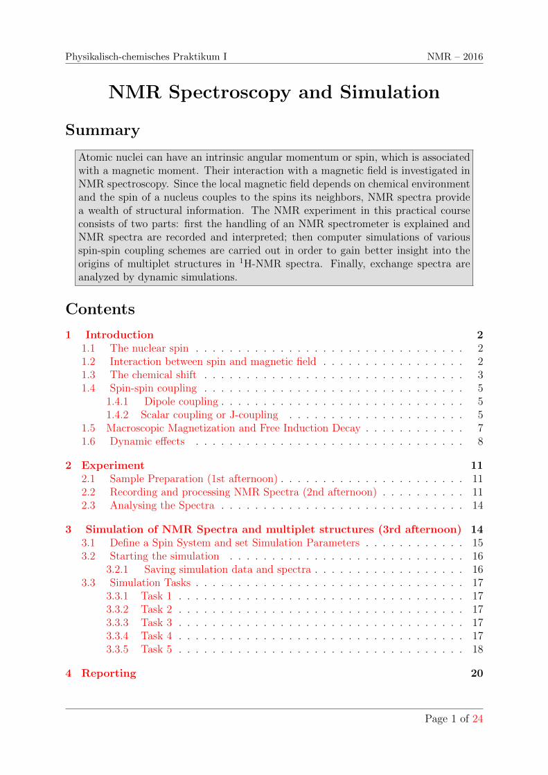
Physikalisch-chemisches Praktikum I NMR – 2016

NMR Spectroscopy and Simulation

Summary

Atomic nuclei can have an intrinsic angular momentum or spin, which is associatedwith a magnetic moment. Their interaction with a magnetic field is investigated inNMR spectroscopy. Since the local magnetic field depends on chemical environmentand the spin of a nucleus couples to the spins its neighbors, NMR spectra providea wealth of structural information. The NMR experiment in this practical courseconsists of two parts: first the handling of an NMR spectrometer is explained andNMR spectra are recorded and interpreted; then computer simulations of variousspin-spin coupling schemes are carried out in order to gain better insight into theorigins of multiplet structures in 1H-NMR spectra. Finally, exchange spectra areanalyzed by dynamic simulations.

Contents

1 Introduction 21.1 The nuclear spin . . . . . . . . . . . . . . . . . . . . . . . . . . . . . . . . 21.2 Interaction between spin and magnetic field . . . . . . . . . . . . . . . . . 21.3 The chemical shift . . . . . . . . . . . . . . . . . . . . . . . . . . . . . . . 31.4 Spin-spin coupling . . . . . . . . . . . . . . . . . . . . . . . . . . . . . . . 5

1.4.1 Dipole coupling . . . . . . . . . . . . . . . . . . . . . . . . . . . . . 51.4.2 Scalar coupling or J-coupling . . . . . . . . . . . . . . . . . . . . . 5

1.5 Macroscopic Magnetization and Free Induction Decay . . . . . . . . . . . . 71.6 Dynamic effects . . . . . . . . . . . . . . . . . . . . . . . . . . . . . . . . 8

2 Experiment 112.1 Sample Preparation (1st afternoon) . . . . . . . . . . . . . . . . . . . . . . 112.2 Recording and processing NMR Spectra (2nd afternoon) . . . . . . . . . . 112.3 Analysing the Spectra . . . . . . . . . . . . . . . . . . . . . . . . . . . . . 14

3 Simulation of NMR Spectra and multiplet structures (3rd afternoon) 143.1 Define a Spin System and set Simulation Parameters . . . . . . . . . . . . 153.2 Starting the simulation . . . . . . . . . . . . . . . . . . . . . . . . . . . . 16

3.2.1 Saving simulation data and spectra . . . . . . . . . . . . . . . . . . 163.3 Simulation Tasks . . . . . . . . . . . . . . . . . . . . . . . . . . . . . . . . 17

3.3.1 Task 1 . . . . . . . . . . . . . . . . . . . . . . . . . . . . . . . . . . 173.3.2 Task 2 . . . . . . . . . . . . . . . . . . . . . . . . . . . . . . . . . . 173.3.3 Task 3 . . . . . . . . . . . . . . . . . . . . . . . . . . . . . . . . . . 173.3.4 Task 4 . . . . . . . . . . . . . . . . . . . . . . . . . . . . . . . . . . 173.3.5 Task 5 . . . . . . . . . . . . . . . . . . . . . . . . . . . . . . . . . . 18

4 Reporting 20

Page 1 of 24


5 Appendix 21

A Sample Preparation - NMR Service 21

B Chemical shifts of some common solvents 22

C Reporting NMR Data in Chemical Documents 23

1 Introduction

1.1 The nuclear spin

An atomic nucleus consists of protons and neutrons. Unless the number of both protonsand neutrons is even, it has an intrinsic magnetic moment, associated with a quantitycalled spin and a quantum number I 6= 0. With an even number of protons and an oddnumber of neutrons or vice versa, the nucleus has a half-integer spin (I = 1/2 for 1H,13C, 19F, 15N, I = 5/2 for 17O). If the numbers of protons and neutrons are both odd, aninteger spin results (I = 1 for 2H, 14N, I = 3 for 10B).

The spin quantum number I is associated with an angular momentum ~I of magnitude

|~I| = ~√I(I + 1) (1)

and an intrinsic magnetic magnetic moment of the nucleus

~µ = γ ~I (2)

The proportionality constant γ is called nuclear gyromagnetic ratio, which is different fordifferent kinds of nuclei and is determined experimentally. For Hydrogen atoms γ(1H) =26.7522 ×107 rad(ians) s(econds)−1T(esla)−1, for 13C, γ(13C) = 6.7283 ×107 rad s−1T−1.

1.2 Interaction between spin and magnetic field

When an external B-field defines a preferred direction (usually chosen to be z), the compo-

nent Iz of the angular momentum vector ~I cannot take arbitrary values but is quantized.It must be either an integer (if I is integer) or all half-integer (if I is half-integer) multipleof ~. Possible components are thus

mI = Iz/~ = I, I − 1, . . . , 0, . . . ,−(I − 1),−I for I integralmI = Iz/~ = I, I − 1, . . . , 1

2,−1

2, . . . ,−(I − 1),−I for I half-integral

yielding 2I + 1 components in each case. The nuclear magnetic dipole components alongthe magnetic field direction are determined by the Iz components:

µz = γIz (3)

and the interaction energy between a magnetic dipole and a field of strength Bz along thez-axis is given by:

E = µz Bz (4)

Page 2 of 24


As a result, there only 2I + 1 discrete energy levels for a spin I nucleus in an externalfield. At vanishing field strength, all levels have the same energy. This degeneracy is liftedwhen the external magnetic field is made stronger, as illustrated in Figure 1 for nucleuswith I = 1.

+1

-1

0

No field

Field in z-direction

��/ℏ

Δ�

0

+�ℏ

−�ℏ

B00

Energy

Figure 1: The three energy levels allowed for a nucleus with spin quantum numberI = 1.

In the following, we will always assume that the applied magnetic field points in thez-direction and has the magnitude B0. The energy difference between two levels with(|∆Iz/~| = 1) is then given by:

∆E = EmI− EmI−1 = γ~

Iz~B0 − γ~(

Iz~− 1)B0 = γ~B0 (5)

The transition of a spin between energy levels is associated with the emission or absorptionof energy in the form of radiation with angular frequency ω given by:

ω =∆E

~= γB0 (6)

The frequency is thus proportional to the applied magnetic field. This is the basis ofnuclear magnetic resonance (NMR) spectroscopy: If we take a hydrogen atom (γ (1H)=26.7522× 107 rad s−1 T−1) in a magnetic field B0 = 3 T, the frequency is:

ν =ω

2π=

3 · 26.7522× 107

6.28319s−1T−1T ≈ 128× 106Hz (7)

This shows that transitions between different spin states of protons in a static magneticfield typical for NMR spectrometers can be induced by electromagnetic radiation of theorder of 100 MHz, corresponding to short-wave radio frequencies.

1.3 The chemical shift

We now consider a nucleus that is part of a molecule. The external magnetic field B0

interacts with the molecule’s electrons. This interaction (you may think of it as a ringcurrent created when the field is switched on) induces a magnetic field opposing the

Page 3 of 24


OH

Increasing Field

Δ�

ℏ= 100.00MHz

CH3

CH3

OH

�Transition frequency

OH CH3

Figure 2: Effect of an external static magnetic field on the energy levels of two protons withdifferent shielding constants.

applied field (diamagnetic circulation). The total field experienced by a nucleus becomesthus:

Beffective = B0 −Binduced (8)

The induced field is proportional to the applied field (Binduced = σB0) where σ is aconstant. For the effective field, we can thus write:

Beffective = B0(1− σ) (9)

The nucleus is thus shielded from the applied field B0 by a diamagnetic ring current ofthe electrons. The extent of this shielding will vary with the local electron density in amolecule and can thus be different for every nucleus in the molecule. For nucleus i withshielding constant σi we write:

Bi = B0(1− σi) (10)

Example: How does the transition frequencies of a proton in an O-H bond differ fromthat in a C-H bond of a methyl group? Since oxygen is more electronegative than carbon,the electron density around the proton of the C-H bond must be larger than that aroundthe proton of the O-H bond. We thus expect σC−H > σO−H and thus

BC−H = B0(1− σC−H) < BO−H = B0(1− σO−H) (11)

The field experienced by the proton of the O-H bond is thus greater than that experiencedby the proton of the C-H bond. This causes a larger splitting of the energy levels of theO-H proton than of those of the C-H proton. The level splitting as a function of increasingexternal static field B0 is depicted in Figure 2. For a given external field the CH3 protonscan be excited at 100.00 MHz, but higher frequency radiation is needed to excite the O-Hprotons.

Hence, spin resonances of the same kind of nucleus (proton) can be observed at differentfrequencies when they are in different chemical environments. The separation betweenthe associated peaks in an NMR spectrum is called the chemical shift. Combiningequations 6 and 10 we obtain for the chemical shift δ:

δ[Hz] = νC−H − νOH =γB0

2π(σC−H − σO−H) (12)

Page 4 of 24


A chemical shift defined in this a way depends, however, on the static magnetic field B0

and thus on the spectrometer. It is more useful to report chemical shifts as a fraction ofthe applied field and relative to a reference proton:

δ[ppm] =ν − νrefνref

× 106 (13)

where ppm means parts per million. This unit is useful because absolute chemical shiftsδ[Hz] are typically of the order of 100 Hz, compared to the 100 MHz transition frequencies.As a reference, the proton signal of TMS (tetra methyl silane, Si(CH3)4) is used byconvention.

Nuclei with identical chemical shifts (same environments) give rise to resonances at thesame frequency. The area of a peak is therefore proportional to the number of equivalentnuclei.

1.4 Spin-spin coupling

1.4.1 Dipole coupling

If two spin-carrying nuclei are close enough, their magnetic moments can influence eachother appreciably via the dipole-dipole interaction. This is also called direct coupling anddepends on the positions of the magnetic moments in space. It can be very large for agiven geometry, but in solution or in the gas phase the effect is averaged out due to fastmolecular motion (rotational diffusion). Solids, on the other hand, must be rotated veryquickly (magic angle spinning) in order to suppress the effect of direct coupling, whichwould otherwise strongly broaden the NMR spectra.

1.4.2 Scalar coupling or J-coupling

Two (magnetically non-equivalent) nuclei also interact via the bonding electrons. Thiseffect is not averaged out by molecular motion and is smaller by about a factor of 102

to 104 than direct coupling and decreases rapidly with the number of bonds separatingthe spins. Since the spin of a proton A can have two possible orientations relative to anexternal field B0, the field BX at a neighboring proton X is either slightly raised or slightlylowered, leading to a splitting of the energy levels. The energies are shifted by

δEAX = h JAXmAmX (14)

where mA = I(A)z /~ is the projection of the spin of nucleus A onto the z-axis. The coupling

constant JAX is usually given in Hz. It can be positive or negative and its magnitude istypically < 20 Hz for proton-proton coupling. When a neighboring proton A is in theupper state (spin up, mA = +1/2), the energy of the lower state of proton X (spin down,mX = −1/2) is thus lowered by δEJ = −h J/4 , while the upper state of proton X is raisedby the same amount of energy. For illustration look at the right-hand side of Figure 3, withorange spins representing proton A and blue arrows representing proton(s) X. Overall, fora spin-up neighbor, the energy gap has increased by h J/2 and the resonance frequencyis raised by J/2. A spin-down neighbor (mA = −1/2) has the opposite effect, raising theenergy of the lower state of X and reducing that of the upper state. The corresponding

Page 5 of 24


resonance frequency is lowered by J/2. As a result, the frequency separation between thetwo peaks of the resulting doublet is simply J .

J

Transition frequencyCOH CH3

1:3:3:1 12:12

J

h�

�

J

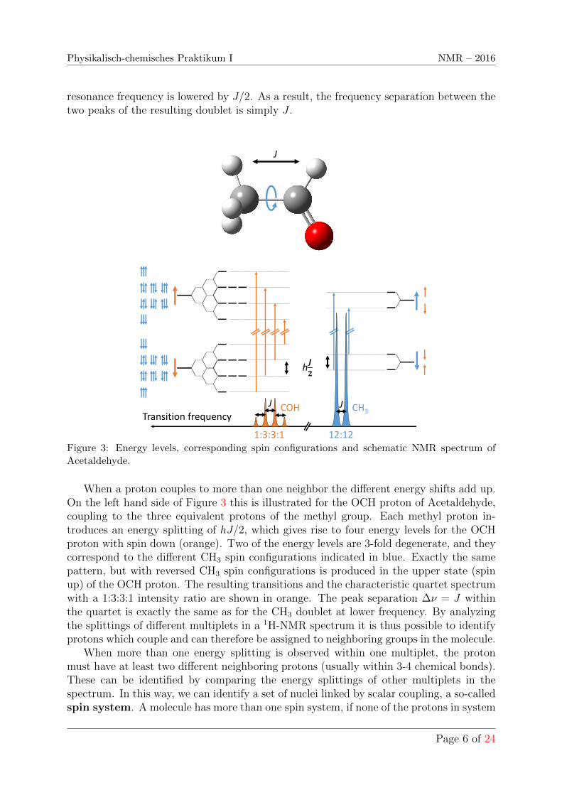
Figure 3: Energy levels, corresponding spin configurations and schematic NMR spectrum ofAcetaldehyde.

When a proton couples to more than one neighbor the different energy shifts add up.On the left hand side of Figure 3 this is illustrated for the OCH proton of Acetaldehyde,coupling to the three equivalent protons of the methyl group. Each methyl proton in-troduces an energy splitting of hJ/2, which gives rise to four energy levels for the OCHproton with spin down (orange). Two of the energy levels are 3-fold degenerate, and theycorrespond to the different CH3 spin configurations indicated in blue. Exactly the samepattern, but with reversed CH3 spin configurations is produced in the upper state (spinup) of the OCH proton. The resulting transitions and the characteristic quartet spectrumwith a 1:3:3:1 intensity ratio are shown in orange. The peak separation ∆ν = J withinthe quartet is exactly the same as for the CH3 doublet at lower frequency. By analyzingthe splittings of different multiplets in a 1H-NMR spectrum it is thus possible to identifyprotons which couple and can therefore be assigned to neighboring groups in the molecule.

When more than one energy splitting is observed within one multiplet, the protonmust have at least two different neighboring protons (usually within 3-4 chemical bonds).These can be identified by comparing the energy splittings of other multiplets in thespectrum. In this way, we can identify a set of nuclei linked by scalar coupling, a so-calledspin system. A molecule has more than one spin system, if none of the protons in system

Page 6 of 24


1 couples to any of the protons in system 2.Simple splitting patterns as in Figure 3 are only found when the difference in transition

frequency of the coupling protons is clearly larger that the coupling constant J . In thatcase one speaks of AiXj type coupling; in the case of CH3-COH of an AX3 type. Ifthis condition is not fulfilled the spectrum turns into a AiBj type spectrum. Indeed,equation 14 is only an approximation, and must be replaced by the full expression

δEAB =2π

~JAB~IA · ~IB =

2π

~JAB

(I(A)x I(B)

x + I(A)y I(B)y + I(A)z I(B)

z

). (15)

The additional contributions of the x and y components of the magnetic moments canlead to very complicated, so-called higher order spectra. If two protons are chemicallyequivalent but exhibit different couplings to other protons (the protons become thenmagnetically non-equivalent), the system is called AA’BB’ type. Note that the transitionfrequency (the chemical shift) depends on the strength of the applied external magneticbut the splitting caused by J coupling does not. Hence, higher magnetic fields can turna complicated AB-type spectrum into a simple AX spectrum.

1.5 Macroscopic Magnetization and Free Induction Decay

In an NMR experiment, a whole ensemble of spins is probed at the same time. The sumof the magnetic moments of all the nuclei is called the magnetization ~M =

∑i ~µi. If we

label the two states of a spin 1/2 nucleus α and β, the z-component of the magnetizationis thus

Mz0 = Nαµzα +Nβµzβ. (16)

Nα and Nβ denote the occupation of the spin states α and β and µzα and µzβ are thez-components of the respective magnetic moments. Using Boltzmann statistics we canwrite

Nα

Nβ

= exp

(− hν

kBT

)(17)

At room temperature kBT/h ≈ 6 GHz (6 · 1012 Hz), while ν is of the order of 108 Hz.As a result, the ratio Nα/Nβ is very close to one. The two levels are therefore nearlyequally populated, even in a very strong magnetic field, and we are always in the hightemperature limit (hν � kBT ) . In this case, the difference in occupation numbers is

∆N0 = Nα −Nβ =N∆E

2kBT= N

γ ~B0

2kBT(18)

where N = Nα + Nβ is the total number of spins. With µzα = −µzβ = γ~/2 we obtainthe equilibrium magnetization

Mz0 = Nγ2~2B0

4kBT(19)

which is also known as Curie’s law.While the static magnetic field B0 causes a net orientation of the spins in the z-

direction, the magnetization in the xy-plane is zero. Irradiating the probe with a ra-diofrequency field with a magnetic component of amplitude B1 in the xy-plane, i.e. per-pendicular to B0, causes transitions between spin states if the frequency of B1 corresponds

Page 7 of 24


�

��

��

�

Transmitter

+Receiver

coil

(�)

�

RF pulse

Fourier

Transform

Figure 4: Schematic principle of Fourier Transform NMR

to the energy splitting between them. So-called superposition states (a|α〉+ b|β〉) are cre-ated, which cause the individual magnetic moments to precess about the z-axis with theLamor frequency

ω = γ B0 (20)

Modern NMR experiments are based on the pulse or Fourier transform (FT) technique.Here, the probe is exposed to a strong, short radiofrequency pulse of a few µs. Theinduced xy-components of the individual magnetic moments initially all point into thesame direction and start to precess at the same time. As a result, the macroscopicmagnetization also acquires a component the xy-plane, which precesses about the z-axiswith the Lamor frequency, as shown in Figure 4. The precessing macroscopic magneticdipole induces an oscillating current in the detection coil of the spectrometer which isdetected as a signal as function of time. When the radiofrequency pulse is switched off,slightly different Lamor frequencies (energy gaps) of the individual spins cause a steadyreduction of the macroscopic magnetization in the xy-plane (dephasing). In addition,the decay of the superposition states and return to the equilibrium population of thespins causes a decay of xy-component of ~M . The corresponding decay of the detectioncoil signal is called free induction decay (FID). Fourier transformation of this signalreveals the NMR spectrum.

The relaxation times T1 and T2 determine the width of the spectrum. T1, the so-called longitudinal relaxation time, is the time it takes to re-establish the equilibriumdistribution of spins in the higher and lower energy states as energy is dissipated to theenvironment. Transverse relaxation with time constant T2 is due to the dephasing of thespins, which initially precess together but then become uncorrelated because of slightlydifferent frequencies due to different (and fluctuating) local environments.

1.6 Dynamic effects

For the structure shown in Fig. 3 the coupling of the OCH proton with the methyl protonin the trans position should be different from the coupling with the other two methylprotons. However, as indicated by the arrow around the C-C bond, the methyl group can

Page 8 of 24


quickly rotate, which leads to three effectively equivalent nuclei with the same (average)coupling constant. What does ’quickly’ or ’fast’ exactly mean in this case? Differences intransition frequencies between protons in different environments are very small and aretypically of the order of 1 ppm (400 Hz on a 400 MHz Spectrometer) or less. In order toresolve a frequency difference δν, we need to be able to measure a signal for longer than

t '1

δν(21)

i.e. t > 10 ms for δν = 100 Hz. If the lifetime τ of the structure giving rise to thesignal becomes smaller than 1/δν, the two frequencies cannot be resolved anymore andan average spectrum is measured. For a simple chemical reaction like A→ B or A B,τ corresponds to 1/kA→B. This effect makes NMR spectroscopy a useful tool for kineticinvestigations of intramolecular processes like the equilibrium between conformers or tau-tomers. For this purpose NMR spectra must be recorded in a wide range of temperatures.

The temperature dependence of a chemical reaction can be analyzed in different ways.In the simplest case, one can use the Arrhenius equation

k = A · exp

(− EaRT

)(22)

or, in logarithmic form:

ln k = lnA− EaR

1

T(23)

Plotting ln k versus 1/T reveals the activation energy Ea and the frequency factor Aunder the assumption that both parameters are temperature independent. The Eyringequation

k = κkBT

hexp

(−∆G

RT

)(24)

is derived from transition state theory and introduces a linear temperature-dependenceof the prefactor. Using ∆G = ∆H −T∆S and numerical values for the natural constantsin SI units, the equation can be transformed into:

log10

k[s−1]

T [K]= 10.32− ∆H[J mole−1]

19.13

1

T [K]+

∆S[J mole−1]

19.13(25)

which can again be evaluated by linear regression. κ is the so-called transmission coeffi-cient and is usually set to 1.

For an accurate analysis of kinetic processes with NMR spectroscopy, the line shapesof the signals must be taken into account, which may become quite complicated. How-ever, computer programs for simulating spectra exist. A suitable strategy is to simulatespectra at different temperatures with varying rates k(T ), until good agreement with theexperimental data is found. The rates corresponding to the best fits can then be usedfor further analysis. For a quick estimate, one can often use the temperature of the spec-trum, at which two bands are just no longer resolved (blue spectrum in Figure 5). Theassociated coalescence rate is given by:

kcoal =π δν√

2≈ 2.22δν (26)

Page 9 of 24


Δ�

Coalescence

Tem

pe

ratu

re Slow

exchange

Fast

exchange

Figure 5: NMR exchange spectrum at different temperatures. Above the coalescence tempera-ture (red line), the two peaks can not be separated anymore.

where δν[Hz] is the difference in frequency of the two bands in the slow exchange limit.By means of the Eyring equation the energy barrier at the coalescence temperature Tcoal

(in K) can now be estimated:

∆G[J mole−1] = 19.13Tcoal

(9.97 + log10

Tcoal

δν

)(27)

Page 10 of 24


2 Experiment

Members of the NMR-Service will demonstrate handling and use of the NMR spectrom-eter. Before the day of the experiment, two samples, previously isolated in the first yearchemistry course, will be handed out to every student and prepared properly. Spectra ofthese probes will be recorded individually after the demonstration and the spectra will beanalyzed. For recording the spectra, the students will have to make reservation for thespectrometer.

2.1 Sample Preparation (1st afternoon)

Before an NMR spectrum can be recorded, the samples have to be prepared appropriately.Please study the ’Merkblatt: Probenvorbereitung’ from the NMR Service, which can befound in the Appendix.

Fill 2-10 mg of your substance into a small vial and dissolve it in about 0.6 ml of thedeuterated solvent handed out by the assistant (0.7 ml in the case of acetone-d6) usingthe dedicated pipettes or syringes. Deuterated solvents are expensive. Please work verycarefully! To test solubility, use non-deuterated solvent. Close the vial and shake it untilyour substance is completely dissolved. Then transfer the solution into an NMR-tube,close the tube thoroughly and label it with your name (or initials), group letter, and thesubstance number.

2.2 Recording and processing NMR Spectra (2nd afternoon)

Spectra are analyzed in the PC lab course using the Bruker software TopSpin. As soonas your measurements are done, come up to the K-floor labs to start the processing.

• For analyzing the spectra on the PCP computers, the data sets are transferred fromthe ftp server to an accessible directory. NMR service will put the data into:

//pcipdc.uzh.ch/praktikum/NMRdata

which should be linked on the computers on which you use the TopSpin software.You should first make personal copies of the data in your subdirectory, but youshould not delete the original files!

• Start the TopSpin program and import your data set. To do that, go to the yellowicon on the top left corner and press OPEN. A pop-up window will allow you tobrowse for your data directories (select Bruker format).

• When you have found the directory with your data, select DISPLAY. The data inthe directory will be imported into the program, processed automatically, and aspectrum will be displayed as shown below:

Page 11 of 24


• By changing the selection in the Menu bar directly on top of the spectrum you can:

view the parameters used for processing the raw data

view the acquisition parameters (spectrometer)

view and change the title title of the measurement

view a list of all peaks that have been marked

view a list of all integrals that are displayed in the spectrum

view and edit sample information

sketch or upload a molecular structure

view the final plot, which will be printed or saved

view the FID, i.e. the original signal in time

• Depending on the choice on the top menu (PROCESS, ANALYSE, PUBLISH) youhave access to different sub menus. If you choose PROCESS, you can modify allthe things the automatic processing has done for you. It is often a good idea to goto PICKPEAKS in the sub menu and then remove some or all of the automaticallygenerated values. To do this, right-click with the mouse inside the spectrum andselect what you want to do. You may repeat the same thing for the integrals(INTEGRATE sub menu).

• As a first task, check that the frequency axis of your spectrum is calibratedcorrectly. Zoom your spectrum to a region around 0 ppm. A robust method forzooming is to use the button . It allows you to specify the ppm range you want todisplay. Now select the PROCESS menu. Chose CALIB.AXIS and move the cursorto the center of the TMS peak near 0 ppm. Left-clicking opens a pop-up window,where you can manually enter the value 0. This will shift the whole spectrum,placing the TMS peak exactly at 0 ppm. Alternatively, you can choose the solvent

Page 12 of 24


10 9 8 7 6 5 4 3 2 1 0 ppm

1.18

1.17

1.00

1H NMR, 300 MHz, 300 K, 0.1 mmol in 0.6 mL DMSO−d64−Chloro−3−nitrobenzoic acid

131415 ppm

0.79

8.08.28.48.6 ppm

1.18

1.17

1.00

Figure 6: Example for a processed spectrum. Peak shifts (in ppm and Hz) integrals and couplingconstants should also be listed separately.

peak and enter its known ppm value (see Appendix B). Display the full spectrumagain.

• To get accurate positions of the peaks in the spectrum, go to the PICKPEAKSsub menu in PROCESS. Select the icon (second from left). By keeping the leftmouse button pressed you can now mark regions in which the program automaticallydetermines peak positions. Unwanted peaks (e.g. noise) can be removed afterunselecting (click it again). Right-clicking on the unwanted peak or on thedisplayed ppm value then allows you to delete the selected peak.

• Next you should to define the peak integrals. Select the INTEGRATE sub menuand again pick the icon. Mark the ppm range you would like to integrate bykeeping the left mouse button pressed while you move from the left to the rightintegration limit. Deleting integrals works like deleting peak values.

• The main reason for integrating peaks is to find out how many protons contributeto a certain signal. We therefore have to calibrate the area under the peaks.To do so, select a peak or multiplet for which the number of contributing protons isknown (or you may have to guess). Pressing the right mouse button allows you tochoose Calibrate Current Integral. Enter the number of contributing protons in thepop-up menu. All the other integrals in the spectrum will be scaled accordingly.

It may now be a good idea to press the return icon (rightmost button on top of thespectrum) and display the full spectrum. You should see all marked peaks and integrals.You can also view them in table form using the Menu bar directly on top of the spectrum.In the peak table, it is important that not only the ppm values, but also the frequencies(in Hz) are shown, in order to be able to determine coupling constants more precisely. Toadd a column with frequencies, right-click on the title row of the table and tick v(F1)Hz.Other parameters may be added or removed in the same manner.

Page 13 of 24


Chemical shift (ppm)

012 10 8 6 4 2

Figure 7: Proton chemical shifts in CDCl3. For more detailed charts consult for example ref. 3.(Source: http://www.cem.msu.edu/∼reusch/OrgPage/nmr.htm).

Multiplet structures can not be seen clearly when looking at the full spectrum. Youshould therefore create additional plots for each multiplet as shown in the example inFigure 6. The different plots can either be assembled within the TopSpin software or inan external program.

2.3 Analysing the Spectra

As a first step, identify all peaks due to solvent and impurities. A very useful table ofcommon signals can be found in Appendix B. The two substances you measured have beenseparated by you in your first year laboratory class. Your observations there can alreadygive you a first hint about their nature (polar, non-polar etc.). This information, togetherwith charts like the one in Figure 7, should facilitate a first assignment of some of the peaksin your spectrum. Next, analyze all multiplets and calculate the coupling constants. Usethese to identify different spin systems and to draw hypothetical (sub-)structures. Checkthe consistency with the peak integrals and recalibrate if necessary. Depending on thecomplexity of your spectrum, you may be given some additional information.

3 Simulation of NMR Spectra and multiplet struc-

tures (3rd afternoon)

For the simulation of NMR spectra we use the program SpinWorks 4, an open sourceNMR analysis program by Kirk Marat, which you can download from the University ofManitoba (windows or Linux):[5]

ftp://davinci.chem.umanitoba.ca/pub/marat/SpinWorks/

You can also use this program to analyze experimental NMR data. It offers fewer optionsthan the Bruker software but it is relatively simple to use. After starting the program,first go to Options/Set Start Options and make sure, the External Module Path points to

Page 14 of 24

ftp://davinci.chem.umanitoba.ca/pub/marat/SpinWorks/


Figure 8: Window for entering a spin systems for simulations with the program SpinWorks 4 (2equivalent ortho, meta and 1 para proton).

the directory where SpinWorks is installed. If you make changes here, close and re-startthe program.

3.1 Define a Spin System and set Simulation Parameters

• Got to the Menu SpinSystem/Edit Chemical Shifts. . . and enter the spin parame-ters in the following fields:

Spins: enter 1 for single protons, 2 for two equivalent protons (CH2), 3 for CH3

etc. In a ring system, two symmetric protons are written as 2*1 (e.g. the two metaprotons of chlorobenzene)Label: give a useful name, e.g. Hmeta, CH3, OCH etcSpecies: make sure you give the same number to all coupled protons. Differentspecies labels mean weak coupling approximation.Spin: choose appropriate spin (1/2) for protonsShift: specify shift in Hz or ppm. The frequency can be changed in the SpinSys-tem/Edit Simulation Options and DNMR Parameters. . . menu (see below)

• Now open the menu SpinSystem/Edit Scalar (J) Coupling. . . and enter the couplingconstants in Hz. Having chosen good labels in the previous step will help here.

• Finally go to SpinSystem/Edit Simulation Options and DNMR Parameters. . . . Hereyou can set the linewidth of the peaks calculated by the simulation program, andthe window in which data will be generated. You can also change the frequency ofthe Spectrometer. If you do that, check under SpinSystem/Edit Chemical Shifts. . .that your peaks are still where you wanted them to be! The right hand side of thismenu will become important only when we simulate exchange spectra.

Page 15 of 24


Figure 9: Window for setting linewidth, plot window and spectrometer frequency in the programSpinWorks. On the right hand side parameters for exchange simulations can be entered.

3.2 Starting the simulation

Make sure that Simulation/Simulation Mode is set to NUMMRIT, then start the calcu-lation by selecting Simulation/Run NUMMRIT Simulation. Alternatively, you can opena popup menu by clicking on the yellow Simulation button in the bottom left corner andrun NUMMRIT from there. After a short moment a simulated spectrum should appearon the screen.

3.2.1 Saving simulation data and spectra

This is probably the least evident and a little tedious aspect of the program. There arein fact many different ways to save (partial) information:

• File/Save Spin System As allows you to save the simulation settings (frequencies,couplings etc). Loading these parameters again later allows you to quickly repeatthe calculation.

• Simulation/List Simulation Output - saves data (peak position and intensities) fromwhich a spectrum could be constructed.

• File/Print to File allows you to print the current window for example to a .pdfprinter

• Edit/Copy Metafile to File does essentially the same more directly, generating awindows metafile to use in your report

• View/Copy Simulated To Experimental copies the simulated spectrum to the exper-imental spectrum. You can then use File/Dump XY Points to File to save ASCIdata for display in an external program or File/Save As(JCAMP DX) to save thespectrum in a more tedious format, which can, however be read again by the pro-gram.

Page 16 of 24


3.3 Simulation Tasks

3.3.1 Task 1

Simulate a spectrum of a molecule with three protons with a chemical shift of 2.2 ppmand one proton with a chemical shift of 9.8 ppm. These chemical shifts correspond toacetaldehyde or ethanal, which we have already discussed above (see Figure 3). A couplingconstant of 20 Hz is assumed. Due to this coupling, the signal of the methyl group is splitinto a doublet and that of the OCH proton into a quartet. The spin system correspondsto an AX3 system.

• The coupling constants is set to ±20.0. What happens to the spectrum if the signof coupling is changed?

• Change the chemical shift of the A-proton, moving it closer to the X3 protons.Document your observations by saving some spectra and discussing them.

3.3.2 Task 2

Here, we investigate some different coupling schemes. We assume, an X-proton is nowcoupled to three distinct protons A, B, and C, which have all much smaller chemical shifts.Observe how the spectrum changes when the coupling constants (ABC)-X are changed.Try the following combinations:

a) J(A,X) = J(B,X)=J(C,X)b) J(B,X) and J(C,X) ≈ J(A,X)c) J(B,X) = J(A,X)/2 and J(C,X) = J(B,X)d) J(A,X) = J(B,X) and J(C,X) = J(A,X)/2e) J(A,X) = J(B,X) and J(C,X) = J(A,X)/4f) J(B,X) = J(A,X)/4 and J(C,X) = J(B,X)g) J(A,X) = J(B,X) + J(C,X)

3.3.3 Task 3

Here we simulate the NMR spectra of an ABXY system at different magnetic fieldstrengths. The chemical shifts are chosen as follows: δA = 1.1 ppm, δB = 1.2 ppm,δX = 9.0 ppm, and δY = 10.0 ppm. Coupling parameters are given in the table below.When you change the spectrometer frequency in the SpinSystem/Edit Simulation Optionsand DNMR Parameters window, make sure to maintain a constant spectral window (inppm), by adjusting the two fields above. Can the calculated spectrum be explained us-ing different spin coupling schemes? What happens upon increasing the strength of themagnetic field? Start with a 60 MHz Spectrometer and move up to 100, 300, 500 and 900MHz.

3.3.4 Task 4

We now investigate a dynamical system.

• Choose a new simulation method by selecting: Simulation/Simulation Mode/MEXICO

Page 17 of 24


B X YA 10 5 5B 5 5X 8

Table 1: Coupling parameters for task 3.

• In the SpinSystem/Edit Simulation Options and DNMR Parameters menu set thecorrect frequency for the spectrometer (500 MHz).

• The Permutation vector 2 should be 2 1 0 0 (since spin 1 (A) exchanges with 2 (B)and 2 with 1 and we have only 2 spins).

• The AB-part of the spectrum as a function of the temperature is shown in Figure 10.Set the chemical shift of the two spins A and B and their coupling according to thisFigure.

• Run the simulation by selecting Simulation/Run MEXICO Simulation. Begin atthe lowest temperature and choose a linewidth (1/T1 is the width for MEXICO)and a kinetic constant k such that the corresponding spectrum in Figure 10 is nicelyreproduced. Keep the line width fixed and change k such that the spectra at theindicated temperatures are also well reproduced. Note your best value of k at eachtemperature.

• Determine the energy barrier between the two states of formamide from an Arrheniusplot and the free energy barrier using equation 25.

Important:

• for the exchange simulations chemical shifts should be set to Hz before closingthe SpinSystem/Edit Chemical Shifts window.

• before changing the rate constant for a new simulation, you can copy the previousone to a stack in View/Copy Simulated To Stack.

• Select View/Copy Simulated To Experimental in order to be able to save the simu-lated spectrum in ASCI form. Use a new Workspace for every new rate constant.

• Save your spin system (File/Save Spin System As) in order to be able to re-loadparameters quickly.

3.3.5 Task 5

Choose at least two spin systems in the molecule(s) you have investigated experimentallyand simulate their spectra with the correct shifts and coupling constants. Plot theoreticaland experimental spectra on the same scale. To do this, load your experimental spectruminto SpinWorks:

Page 18 of 24


N+

O

HHA

HB

N

O

HHA

HB

6.6 6.8 7.0 7.2 7.4 7.6 7.8

293 K

303 K

313 K

323 K

333 K

343 K

353 K

363 K

366 K

368 K

370 K

372 K

374 K

379 K

Chemical Shift (ppm)

DMSO

Figure 10: 1H-NMR spectra of the amide protons of formamide in DMSO at different tempera-tures, recorded on a 500 MHz spectrometer.

Page 19 of 24


Options/Data Format select BrukerFile/Open find appropriate file called fidProcessing/Window + FT + Phase you should see your phased spectrum

When you now open the Spin System menu you will see that your frequency has beenautomatically set to the experimental one. Choose your chemical shifts and couplings ina reasonable way, based on your previous analysis and data in ref. 3. Use the NUMMRITsimulation again to compute spectra. Refine your parameters until you get a good match!Note: It is now actually possible (and not too difficult) to fully fit your spectrum. If youare interested in doing this read the SpinWorks documentation and try it out!

4 Reporting

• Hand in a single report, comprising experimental spectra, their analysis and thesimulations, but start working on it before the day you do the simulations!

• In the introduction, briefly describe how you obtained the samples in you first yearlab course and the goal of the current experiments.

• The experimental spectra must be clearly readable (enlarged multiplet structures)and accompanied by a complete list of chemical shifts and integrals.

• All peaks must be (tentatively) assigned. You should outline your reasoning leadingto these assignments. This is more important than coming up with the correctstructure! Specify the coupling schemes (ABX, AABB, etc.) leading to the observedpeaks. You should use the simulated spectra (in particular Task 5) to support yourarguments.

• The simulation work needs to be an independent part of the report. Place it in aseparate section and explain your analysis (steps, equations). Do not forget properunits!

• For at least one substance, practice compliance with the rules of scientific journalsby providing a proper listing of your NMR data. Follow (as far as possible) theinstructions in the Appendix C at the end of this document, taken from the Manualfor Writing Chemical Documents by Prof. S. Bienz.

Page 20 of 24


5 Appendix

A Sample Preparation - NMR Service

- 1 -

NMR-Laboratorium des Instituts für Chemie Universität Zürich Irchel, Winterthurerstrasse 190, 8057 Zürich

Merkblatt : Probenvorbereitung

Probenmenge und Lösungsmittel:

Konzentration der Lösung für Standard-1H-Messungen: 0.01 mol/l

Konzentration der Lösung für Standard-13C-Messungen: 0.10 mol/l

Die Länge des NMR-Röhrchens muss mindestens 17 cm betragen. Die Qualität der NMR-Röhrchen spielt keine grosse Rolle. Es können also ohne Probleme die Economy-Röhrchen auch für die Hochfeld-Geräte verwendet

werden. Bei sehr geringen Substanzmengen sollte ein Shigemi-Röhrchen benutzt werden. Das Glas dieser

Röhrchen hat die gleiche magnetische Suszeptibilität wie das Lösungsmittel. Shigemi-Röhrchen für Methanol, DMSO, Wasser, und CDCl3 können bei uns kostenlos ausgeliehen werden. Der Preis für ein Shigemi-Röhrchen

beträgt im Handel ca. CHF 100.- .

Es sind deuterierte Lösungsmittel zu verwenden, wobei folgende Lösungsmittel zu Verfügung gestellt werden:

CDCl3, DMSO-d6, Methanol-d4, Aceton-d6, Benzol-d6, D2O; weitere Lösungsmittel nur auf Anfrage. Die Lösungsmittel sind in unterschiedlicher Qualität verfügbar. Für kleine Probenmengen sollte ein Deuterierungs-

grad von >99.9 % verwendet werden.

Die Substanz muss vollständig gelöst sein. Die Lösung ist durch Filtration von Feststoffen und Fasern zu befreien, da diese das Shimmen stark erschweren bis verunmöglichen. Speziell beim Shigemi-Röhrchen muss

darauf geachtet werden, dass das Probenvolumen absolut blasenfrei ist. Das kann durch schnelles Antippen des Stempels erreicht werden. Um die CDCl3-Lösung blasenfrei zu haben, braucht es gewisse Praxis. Eine

grössere Menge an gelöstem Sauerstoff kann das Shimmen erschweren oder gar verunmöglichen. Das ist oft

der Fall, wenn das Lösungsmittel schnell mit Gilsonpipetten transferiert wurde. In diesem Fall hilft das Benützen des Ultraschallbades, um den Sauerstoff zu entfernen.

Füllhöhe:

Die Füllhöhe von 4.0 cm ist unbedingt einzuhalten. Dies entspricht einer Füllmenge von mindestens 500 l,

besser sind 600 l. Geringere Füllhöhen erschweren das Shimmen. Im Shigemi-Röhrchen wird die Substanz in

280 l Lösungsmittel gelöst.

Beschriftung der NMR-Röhrchen:

ALLE NMR-Röhrchen müssen gut verschlossen und beschriftet sein. Der Samplecode kann auf farbigem

Klebeband angebracht werden. Aber keine Fähnchen, welche das Absenken des Samples in den Magneten

und das Drehen des Röhrchens beeinträchtigen. Zusätzlich ist beim Shigemi-Röhrchen das innere Röhrchen mit Parafilm oder Teflonband auf der entsprechenden Höhe am äusseren Röhrchen zu fixieren.

Spinner

Die Spinner, die für die NMR-Messungen verwendet werden, sind nicht lösungsmittelbeständig. NMR-Röhrchen

dürfen nicht im Spinner mit Lösungsmittel aufgefüllt werden!

Referenzierung: Allgemein gilt: Für eine richtige Referenzierung der Spektren muss die Probe TMS enthalten. Wir empfehlen,

das TMS nicht direkt ins Röhrchen zu geben, sondern dem CDCl3 in der persönlichen Vorratsflasche 3 Tropfen

TMS zuzufügen. Wird TMS direkt zur Probe zugegeben, sollte die Pipette nur aus der Gasphase über dem TMS gefüllt werden.

NOE-Messungen:

Für quantitative Ergebnisse und bei kleinen Molekülen müssen die Proben durch mehrmaliges einfrieren und

evakuieren entgast werden.

Page 21 of 24


B Chemical shifts of some common solvents

The first step when analysing an NMR spectrum is to calibrate the frequency axis and toidentify peaks due to solvent and impurities. The following list of chemical shifts of themost common solvents and impurities was published in the Journal of Organic Chemistryin 1997:[6]

show their degree of variability. Occasionally, in orderto distinguish between peaks whose assignment was

ambiguous, a further 1-2 µL of a specific substrate wereadded and the spectra run again.

Table 1. 1H NMR Dataproton mult CDCl3 (CD3)2CO (CD3)2SO C6D6 CD3CN CD3OD D2O

solvent residual peak 7.26 2.05 2.50 7.16 1.94 3.31 4.79H2O s 1.56 2.84a 3.33a 0.40 2.13 4.87acetic acid CH3 s 2.10 1.96 1.91 1.55 1.96 1.99 2.08acetone CH3 s 2.17 2.09 2.09 1.55 2.08 2.15 2.22acetonitrile CH3 s 2.10 2.05 2.07 1.55 1.96 2.03 2.06benzene CH s 7.36 7.36 7.37 7.15 7.37 7.33tert-butyl alcohol CH3 s 1.28 1.18 1.11 1.05 1.16 1.40 1.24

OHc s 4.19 1.55 2.18tert-butyl methyl ether CCH3 s 1.19 1.13 1.11 1.07 1.14 1.15 1.21

OCH3 s 3.22 3.13 3.08 3.04 3.13 3.20 3.22BHTb ArH s 6.98 6.96 6.87 7.05 6.97 6.92

OHc s 5.01 6.65 4.79 5.20ArCH3 s 2.27 2.22 2.18 2.24 2.22 2.21ArC(CH3)3 s 1.43 1.41 1.36 1.38 1.39 1.40

chloroform CH s 7.26 8.02 8.32 6.15 7.58 7.90cyclohexane CH2 s 1.43 1.43 1.40 1.40 1.44 1.451,2-dichloroethane CH2 s 3.73 3.87 3.90 2.90 3.81 3.78dichloromethane CH2 s 5.30 5.63 5.76 4.27 5.44 5.49diethyl ether CH3 t, 7 1.21 1.11 1.09 1.11 1.12 1.18 1.17

CH2 q, 7 3.48 3.41 3.38 3.26 3.42 3.49 3.56diglyme CH2 m 3.65 3.56 3.51 3.46 3.53 3.61 3.67

CH2 m 3.57 3.47 3.38 3.34 3.45 3.58 3.61OCH3 s 3.39 3.28 3.24 3.11 3.29 3.35 3.37

1,2-dimethoxyethane CH3 s 3.40 3.28 3.24 3.12 3.28 3.35 3.37CH2 s 3.55 3.46 3.43 3.33 3.45 3.52 3.60

dimethylacetamide CH3CO s 2.09 1.97 1.96 1.60 1.97 2.07 2.08NCH3 s 3.02 3.00 2.94 2.57 2.96 3.31 3.06NCH3 s 2.94 2.83 2.78 2.05 2.83 2.92 2.90

dimethylformamide CH s 8.02 7.96 7.95 7.63 7.92 7.97 7.92CH3 s 2.96 2.94 2.89 2.36 2.89 2.99 3.01CH3 s 2.88 2.78 2.73 1.86 2.77 2.86 2.85

dimethyl sulfoxide CH3 s 2.62 2.52 2.54 1.68 2.50 2.65 2.71dioxane CH2 s 3.71 3.59 3.57 3.35 3.60 3.66 3.75ethanol CH3 t, 7 1.25 1.12 1.06 0.96 1.12 1.19 1.17

CH2 q, 7d 3.72 3.57 3.44 3.34 3.54 3.60 3.65OH sc,d 1.32 3.39 4.63 2.47

ethyl acetate CH3CO s 2.05 1.97 1.99 1.65 1.97 2.01 2.07CH2CH3 q, 7 4.12 4.05 4.03 3.89 4.06 4.09 4.14CH2CH3 t, 7 1.26 1.20 1.17 0.92 1.20 1.24 1.24

ethyl methyl ketone CH3CO s 2.14 2.07 2.07 1.58 2.06 2.12 2.19CH2CH3 q, 7 2.46 2.45 2.43 1.81 2.43 2.50 3.18CH2CH3 t, 7 1.06 0.96 0.91 0.85 0.96 1.01 1.26

ethylene glycol CH se 3.76 3.28 3.34 3.41 3.51 3.59 3.65“grease” f CH3 m 0.86 0.87 0.92 0.86 0.88

CH2 br s 1.26 1.29 1.36 1.27 1.29n-hexane CH3 t 0.88 0.88 0.86 0.89 0.89 0.90

CH2 m 1.26 1.28 1.25 1.24 1.28 1.29HMPAg CH3 d, 9.5 2.65 2.59 2.53 2.40 2.57 2.64 2.61methanol CH3 sh 3.49 3.31 3.16 3.07 3.28 3.34 3.34

OH sc,h 1.09 3.12 4.01 2.16nitromethane CH3 s 4.33 4.43 4.42 2.94 4.31 4.34 4.40n-pentane CH3 t, 7 0.88 0.88 0.86 0.87 0.89 0.90

CH2 m 1.27 1.27 1.27 1.23 1.29 1.292-propanol CH3 d, 6 1.22 1.10 1.04 0.95 1.09 1.50 1.17

CH sep, 6 4.04 3.90 3.78 3.67 3.87 3.92 4.02pyridine CH(2) m 8.62 8.58 8.58 8.53 8.57 8.53 8.52

CH(3) m 7.29 7.35 7.39 6.66 7.33 7.44 7.45CH(4) m 7.68 7.76 7.79 6.98 7.73 7.85 7.87

silicone greasei CH3 s 0.07 0.13 0.29 0.08 0.10tetrahydrofuran CH2 m 1.85 1.79 1.76 1.40 1.80 1.87 1.88

CH2O m 3.76 3.63 3.60 3.57 3.64 3.71 3.74toluene CH3 s 2.36 2.32 2.30 2.11 2.33 2.32

CH(o/p) m 7.17 7.1-7.2 7.18 7.02 7.1-7.3 7.16CH(m) m 7.25 7.1-7.2 7.25 7.13 7.1-7.3 7.16

triethylamine CH3 t,7 1.03 0.96 0.93 0.96 0.96 1.05 0.99CH2 q, 7 2.53 2.45 2.43 2.40 2.45 2.58 2.57

a In these solvents the intermolecular rate of exchange is slow enough that a peak due to HDO is usually also observed; it appears at2.81 and 3.30 ppm in acetone and DMSO, respectively. In the former solvent, it is often seen as a 1:1:1 triplet, with 2JH,D ) 1 Hz.b 2,6-Dimethyl-4-tert-butylphenol. c The signals from exchangeable protons were not always identified. d In some cases (see note a), thecoupling interaction between the CH2 and the OH protons may be observed (J ) 5 Hz). e In CD3CN, the OH proton was seen as a multipletat δ 2.69, and extra coupling was also apparent on the methylene peak. f Long-chain, linear aliphatic hydrocarbons. Their solubility inDMSO was too low to give visible peaks. g Hexamethylphosphoramide. h In some cases (see notes a, d), the coupling interaction betweenthe CH3 and the OH protons may be observed (J ) 5.5 Hz). i Poly(dimethylsiloxane). Its solubility in DMSO was too low to give visiblepeaks.

Notes J. Org. Chem., Vol. 62, No. 21, 1997 7513

Page 22 of 24


C Reporting NMR Data in Chemical Documents

The following extract from the Manual for Writing Laboratory Reports,[1] based on anearlier document by Prof. S. Bienz. It should serve as a guideline for summarizing theanalysis of the NMR spectra in your report.

[2–4]

References

[1] G. Artus, S. Bienz, K. Venkatesan, J. Helbing, Handbook on Writing Laboratory Re-ports, Department of Chemistry, University of Zurich, 2016.

[2] O. Zerbe, S. Jurt, Applied NMR Spectroscopy for Chemists and Life Scientists, 1sted., Wiley-VCH, Weinheim, Germany, 2013 [link].

[3] H. Gunther, NMR Spectroscopy - Basic Principles, Concepts, and Applications inChemistry, 3rd ed., Wiley-VCH, 2013 [link].

Page 23 of 24

http://www.wiley-vch.de/publish/dt/books/ISBN978-3-527-32775-1/

http://www.wiley-vch.de/publish/dt/books/ISBN978-3-527-33000-3/


[4] M. Hesse, H. Meier, B. Zeeh, Spektroskopische Methoden in der organischen Chemie,7th ed., Georg Thieme Verlag, Stuttgart, 2005 [link].

[5] K. Marat, SpinWorks Software and Documentation, Version 4.2.4, University of Man-itoba, 2016.

[6] H. E. Gottlieb, V. Kotlyar, A. Nudelman, NMR chemical shifts of common laboratorysolvents as trace impurities, J. Org. Chem. 1997, 62, 7512–7515 [link].

Page 24 of 24

http://www.thieme-connect.de/products/ebooks/book/10.1055/b-002-46985

http://dx.doi.org/10.1021/jo971176v