Embed Size (px)
Citation preview
NMR Course 2009 February 19, 2009 NMR Research Center
61
2009
NMR Research Center
2/25/2009
NMR Experiment Procedure

NMR Course 2009 February 19, 2009 NMR Research Center
62
Experimental Guide for Varian MR Spectrometers
February, 2009 Introduction: NMR Experiment Procedures…………………......1 Exp.1: 1D proton and Basic Operations………………......2 Exp.2: 1D Carbon and Basic Operations………………...10 Exp.3: Proton 90° Pulse Width Calibration………….…..12 Exp.4: Carbon 90° Pulse Width Calibration……….….…14 Exp.5: APT……………………………………………….....15 Exp.6: DEPT………………………………………….….…16 Exp.7: INEPT……………………………………….…..…..18 Exp.8: Presat or Water Suppression Experiment……..…20 Exp.9: Gradient Shim…………………………………..….23 Exp.10: COSY…………………………………………..……26 Exp.11: HETCOR………………………………………..…..28 Exp.12: 1D NOE…………………………………………..….30 Exp.13: CYCLENOE (INOVA System)…………………....31 Exp14: NOEDIF(Mercury 300 Only)………………….…..33 Exp15: NOESY……………………………………………...34 Exp16: HMQC/HMBC………………………………….….35 Exp 17: 2D Data rocessing……………………………….…..38 Exp 18: 1D Carbon with Fluorine Decoupling…………..…43 Exp19: Variable Hi/Lo Temperature Experiments….……45 Exp 20: Solid State NMR: CPMAS…………………….…... Experiments and process procedures on VNMRS400…………………….. 46 Appendix A: How to transfer data from Sun host computers to a PC……61 Appendix B: When and how to use command su acqproc……………….62 Appendix C: Most Useful Commands for VNMR and VNMRJ…………64 Appendix D: Processing NMR data with a PC…………………………..66

NMR Course 2009 February 19, 2009 NMR Research Center
63
Introduction: NMR Experiment Procedures Step 1. Login Varian UNITYINOVA NMR spectrometer is controlled by a host Sun computer. For security and administration reasons, all research groups at Emory University are issued their group usernames and passwords for the host computers. All authorized NMR users must use their group usernames and passwords to login to the host computers. Step 2. Change Sample A sealed CDCl3 standard is always placed in the magnet to keep the instrument in working condition when not in use. Every user needs to replace the standard sample with your own sample at the beginning of each experiment and change back at the end of the experiment. Step 3. Lock and Shim the Magnet Locking the magnet keeps its field constant and stable during data acquisition. Shimming the magnet makes it uniform and homogenous for a sample to get a reasonable resolution and line shape. Step 4. Setup Parameters and Acquire Data Retrieve default parameters that are setup and updated for you by the NMR Center so that you may collect your data efficiently. Change some parameters accordingly to meet your own experiment needs. Step 5. Process Data, Plot Spectrum and Save the Spectrum This step converts data into NMR spectra. After proper processed, you could plot it on paper for your record. Also you should save the spectrum for your future review. Step 6. Logout Your mission is completed and you need to do a few things for the next user. Step 1, 2, 3, and 6 are the same for all experiments. We will describe them in detail in Experiment One. Step 4 and 5 differ from experiment to experiment. Note on NMR Operating Software: Varian INOVA600, INOVA400, UNITY Plus 600, UNITY400: Solaris 8 and VNMR 6.1C on SUN Workstations Varian Mercury 300, Mercury Vx 300 (at WW) VNMRS400 and Rollins V400: RedHat Linux 4.0WS and VNMRJ 1.1D or VNMRJ2.1B on Dell 380N PC Bruker Avance 600WB: IRIS 6.5 (SIG O2) and Xwin-NMR 3.5 Off-line data processing by PC or Mac. NUTS from Acornnmr, Inc. www.acornnmr.com MestReNova 5.01 from www.mestrec.com.

NMR Course 2009 February 19, 2009 NMR Research Center
64
Experiment 1: 1D Proton and Basic Operations Sample to be used: 10% Strychnine in CDCl3
Step 1. Login 1.1 Sign in NMR logbook.
Type in your username at login prompt on the screen. Type in your account password as the screen prompts. Please note both the username and password are case sensitive. If you could not login, contact Dr. Wu. The VNMR software will be loaded in several seconds with the display of four windows. The upper left window is used for entering commands and selecting menu buttons; the middle left for displaying NMR spectra and the lower left for displaying NMR parameters and other text messages. The upper right window is called “ACQUISITION STATUS” window, indicating the working status of the instrument, such as lock level, spin rate, temperature and acquisition time, etc.
Step 2. Change Sample 2.1 Click on Acqi or type acqi in the command line to display the fifth window at lower
right, which is called “ACQUISITION” window. All the operations hereafter in Step 2 and Step 3 will be operated in this window. There are CLOSE, LOCK, FID, SHIM and

NMR Course 2009 February 19, 2009 NMR Research Center
65
LARGE popup menu buttons, and Sample eject and Sample insert buttons. We will be focusing on the LOCK and the SHIM buttons first.
2.2 Click on LOCK button to display lock sub-window then click SPIN: off button to turn
off sample spinning; click LOCK: off to turn off the lock. 2.3 After a few seconds, the spin rate displays zero, then click on the SAMPLE: eject button
to eject the standard sample onto the top of the magnet; remove the spinner, replace the sample with your own, use sample depth gauge to measure the correct tube position, use kimwipes to clean the spinner and your sample, then put the spinner back onto the top of the magnet again. Caution: place the spinner with a sample on top of the magnet only when ejecting air is on.
2.4 Click on the SAMPLE: insert button to put the spinner back down inside the probe. Wait
for 3 to 5 seconds, then click on the SPIN: on button to make the sample spin.
Lock sub-window

NMR Course 2009 February 19, 2009 NMR Research Center
66
Step 3. How to Lock and Shim the Magnet In this step, you need to adjust lock and shim parameters by using the mouse. Each parameter can be increased or decreased by 1, 4, 16 and 64 units as shown by corresponding –1+, -4+, -16+ and –64+ buttons. For example, when you place the cursor on a button, say –4+, if you click the left mouse button once, the corresponding parameter is decreased by 4 units; if you click the right mouse button twice, the parameter is increased by 8 units. 3.1 If you are using CDCl3 solvent, the magnet could be locked almost instantly most of the
time. This is indicated by the display of lock signal plateau and a green LOCKED message below it. Then you directly go to step 3.3.
3.2 If you don’t see a plateau signal with a LOCKED message or you are using solvent other than CDCl3, click on LOCK: off button, adjust Z0 to make wave-like lock signal into plateau-like resonance, then click LOCK: on button. A green LOCKED should be shown. Then adjust the lock phase to make the lock level as high as possible. You need to reduce both the lock power and lock gain several units if the lock level exceeds 100. You may also check our record sheets on the desk. There are Z0, Lock power, Lock gain, and Lock phase values for different solvents recorded by previous users.
3.3 Now it is shimming time. There are as many ways to shim the magnet. We suggest you
shim it this way: 3.2.1 Click SHIM button to display shim sub-window. The lock level is shown in this window
as two color bars and exact lock level is shown underneath the bars. In the middle of the window, there is one triangular button after ‘SHIM:’ which let you switch from shim sub-windows and lock sub-window by just click on it. Now it should show coarse z by the button.

NMR Course 2009 February 19, 2009 NMR Research Center
67
3.2.2 Adjust Z1C (Z1 coarse) and Z2C(Z2 coarse) by alternatively changing 1 or 4 units to
increase the lock level as high as you can. If the lock level increases to 100, decrease lock gain on the bottom of the window and then continue to adjust Z1C and Z2C. Higher lock level indicates better homogeneity of the magnetic field.
3.2.3 Click on the triangular button to switch to fine z sub-window. Adjust Z1, Z2 and Z3 one after another to make the lock level as high as possible, then adjust Z3, Z2, Z1 as such back and forth a couple of times. We do not suggest you to adjust Z4 and Z5 at this stage. If you really want to adjust them, it is better write them down before you change them, so that you are able to go back in the case you get a worse shimming.
3.3 Finally click the CLOSE button to end the shimming procedure.
Tip 1. Retrieve our default standard shimming file.
If you have a very bad shim, type “loadshim” in the command window to reinstall our default shim file for the standard sample. If you would to like to save your good shims, type svs(‘shim_name’). The file will be saved in: /export/home/nmruser/your_ID/vnmrsys/shims. You could reload your shims by changing to the above file folder, select the shim file, then click main file data ( high light the shim file) then click load shim, then type su to use the new shim file.
NMR Course 2009 February 19, 2009 NMR Research Center
68
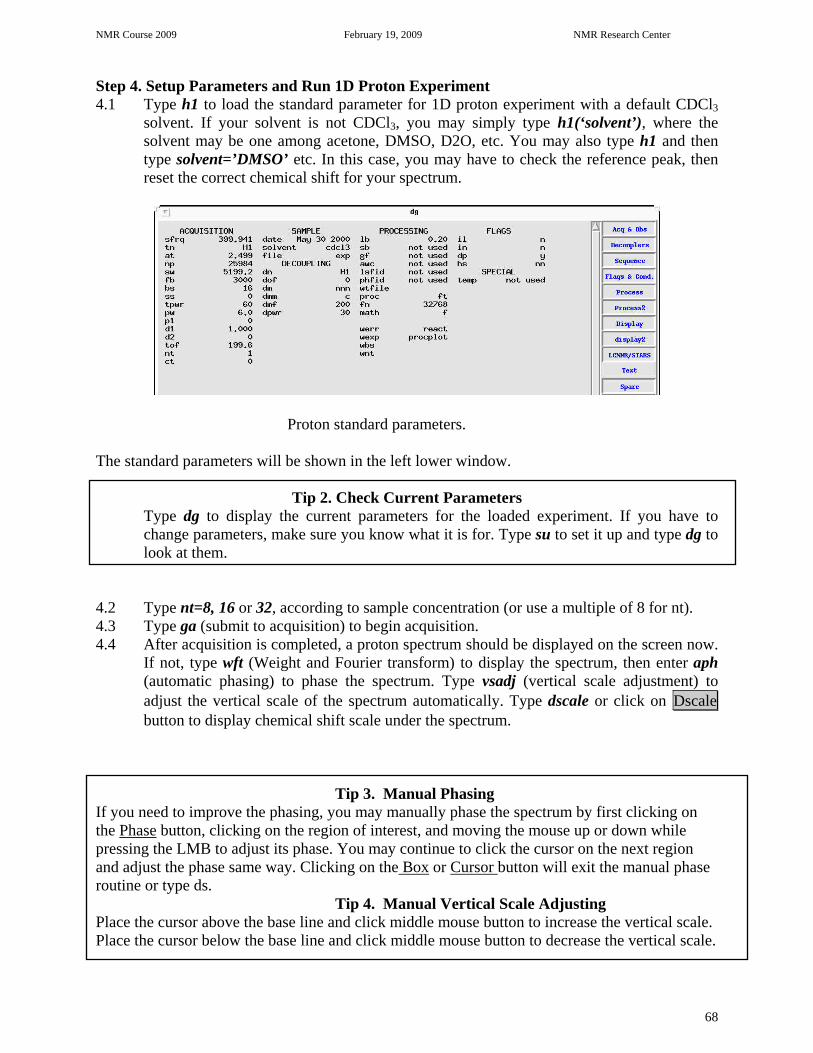
Step 4. Setup Parameters and Run 1D Proton Experiment 4.1 Type h1 to load the standard parameter for 1D proton experiment with a default CDCl3
solvent. If your solvent is not CDCl3, you may simply type h1(‘solvent’), where the solvent may be one among acetone, DMSO, D2O, etc. You may also type h1 and then type solvent=’DMSO’ etc. In this case, you may have to check the reference peak, then reset the correct chemical shift for your spectrum.
Proton standard parameters.
The standard parameters will be shown in the left lower window.
Tip 2. Check Current Parameters Type dg to display the current parameters for the loaded experiment. If you have to change parameters, make sure you know what it is for. Type su to set it up and type dg to look at them.
4.2 Type nt=8, 16 or 32, according to sample concentration (or use a multiple of 8 for nt). 4.3 Type ga (submit to acquisition) to begin acquisition. 4.4 After acquisition is completed, a proton spectrum should be displayed on the screen now.
If not, type wft (Weight and Fourier transform) to display the spectrum, then enter aph (automatic phasing) to phase the spectrum. Type vsadj (vertical scale adjustment) to adjust the vertical scale of the spectrum automatically. Type dscale or click on Dscale button to display chemical shift scale under the spectrum.
Tip 3. Manual Phasing If you need to improve the phasing, you may manually phase the spectrum by first clicking on the Phase button, clicking on the region of interest, and moving the mouse up or down while pressing the LMB to adjust its phase. You may continue to click the cursor on the next region and adjust the phase same way. Clicking on the Box or Cursor button will exit the manual phase routine or type ds. Tip 4. Manual Vertical Scale Adjusting Place the cursor above the base line and click middle mouse button to increase the vertical scale. Place the cursor below the base line and click middle mouse button to decrease the vertical scale.

NMR Course 2009 February 19, 2009 NMR Research Center
69
Step 5. Data Processing 5.1 Zoom operation Click the LMB on the left side and click the RMB on the right side of a peak. Two vertical red cursors will appear at the click points, then click the Expand button on the menu bar. The region between the red cursors will be expanded. Click on Full button to return to the full spectrum after expanding, or type f then press enter. You may do this zooming operation as many times as you like. 5.2 Set reference
After zooming the region containing the reference peak, click the LMB near the top of the peak, then type nl to place the cursor exactly on the top of the peak. Then type rl(x.xxp) to set its chemical shift. For example, rl(4.80p) will set a peak frequency to 4.80ppm.
5.3 Integral operation Enter vp=12 or larger. Type ds cz to clear all the previous integral values in the buffer.
Click on the Part Integral button for the full spectrum or its expanded region to display an integral curve, then click on the Resets button. Now click the LMB at both sides of each peak or integral region to get separated integral lines of the spectrum. If you know the proton number a specific peak represents, you may set the value for that integral as follows: place the cursor on the integral and then click on Set Int. The computer will then ask what value to assign that integral. After you input the value for a particular integral, the computer will recalculate the value of every other integral relatively. You are able to see these values by typing dpir.
Tip 5. Redo integral operation If you made a mistake during the integral operation, you can redo the integral operation by typing cz.
5.4 Peak picking operation
Type ds and click on Th to display a yellow horizontal threshold line. Every peak above this line will be assigned its chemical shift in ppm (axis=’p’) or hz (axis=’h’). Press and hold the LMB to move the yellow cursor to the position you desire, then click on the Th button again. Type dpf to display peak frequencies above spectrum peaks.
Tip 6. Returning to interactive adjustment
During the above operations, if you are not able to find the button you need or you are unable to use the red cursor, simply click on Main menu > Display > Interactive

NMR Course 2009 February 19, 2009 NMR Research Center
70
5.5 Label your experiment data Type ctext to clear any text label for the present experimental data. Type text(‘Your sample name date\\solvent’) to label the present experimental data. Command dtext will display the text on the top left corner of your spectrum.
5.6 Print and plot spectrum and related information
All printing procedure starts with pl and ends with page. You can put other printing commands selectively between these two commands.
ppa--- to print select parameters with text labels. pl--- to print the present spectrum; pap--- to print all the parameters including the text labels, if any. ptext--- to print text labels without other parameters. pscale--- to print the spectrum scale in ppm or hz by axis=“p” or axis=“h”.
ppf--- to print all the peak frequencies over the respective peaks. pll--- to print a list of the frequencies and intensities. pirn--- to print normalized integral values below the respective peaks. pir--- to print proton numbers below the respective peaks. page --- to expel the paper from printer. If you want to print integrals, set vp =12 first, or it wouldn’t print. 5.7 Save your experimental data and reload your experimental data You may save your spectrum data.
The directory path is /export/home/nmrusr/Login_ID/ when you login. It is your group directory. You should make a directory for your own files. Type mkdir(‘yourname’) to make a directory of your own. Type pwd to check the current directory. If it does not, click on Main menu > File then highlight your directory name and click on Set directory. Remember you can go back to your group directory at any time by typing cd. To check the current directory, type pwd. Type svf(’file_name’) to save your data in the form of FID.
5.8. To reload your file, go to your directory first as described above, then click on Main menu > File > highlight your file > click on load. Then type wft.
Step 6. Logout 6.1 Retrieve standard file and replace your sample with the standard.
Type h1 to set up standard proton file. This is especially important after you have done a carbon-13 experiment. It will turn off the decoupling channel automatically.
Then see Step 2 for details about replacing NMR sample tubes. 6.2 Lock and shim the magnet
See Step 3 for details. You are required to shim the magnet to the required level: ‘loadshim’ will reload the current shims for the standard.
6.3 Exit the VNMR program Type exit to close the VNMR program. Now you will see a full screen of Varian’s logo.
6.4 Exit UNIX system

NMR Course 2009 February 19, 2009 NMR Research Center
71
Press the RMB to select Exit item in the popped up menu, release RMB. You will be prompted to select one of two choices: Exit or Cancel. Click on Exit to exit UNIX system. The screen will become blank and a prompt appears.
Caution: It is important to logout completely, otherwise your account will be still charged! Tip: Insert a part of your spectrum on the top of your full spectrum:
1. After the processing completed, type pl pscale no page command, that will save the full spectrum in plotter queue;
2. Use both red cursors to select the area you want to inserted, then type inset, The part of the spectrum will be displayed in the middle of the spectrum. Use mouse to adjust the size and location. Then type pl pscale page.
3. After printing completed, then your type: ds full f and vs=0, you will get the original spectrum back.
4. You could repeat these steps for few times and insert several spectra in the same plot before you type the page command.

NMR Course 2009 February 19, 2009 NMR Research Center
72
Experiment 2: 1D Carbon-13 and Basic Operations
Sample to be used: 30% Strychnine in CDCl3
Step 1. Login (See Experiment One)
Step 2. Change Sample (See Experiment One) Step 3. Lock and Shim The Magnet (See Experiment One) Step 4. Setup Parameters Carbon Experiment 4.1 For Standard C-13 spectrum (Fully decoupled with NOE enhancement): Type c13 or
c13(‘solvent’) to call up the standard carbon-13 experiment parameters with CDCl3 solvent or different solvent.
4.2 Enter nt=128, 256, or more according to the nature of your sample. Type time to check the total time of the experiment.
4.3 Type ga to begin acquisition. 4.5 After acquisition is done, a carbon spectrum should be displayed. If not, enter wft. Type
aph for automatic phasing. Manual phasing is often necessary for a carbon-13 spectrum.
Tip 7. Use large values for nt and aa Commands 13C sensitivity is very low. A common practice is to set a very large number for nt (ex. nt=5000 etc.) to start the experiment. You can check the spectrum by typing wft aph and stop the experiment at any time by typing the aa command to abort acquisition. The time command can be used to estimate the total experiment time with a given nt. Step 5. Data Processing 5.1 Zoom operation
Click the LMB on the left side of a peak and the RMB on the right side. Two vertical red cursors will appear at the click points, then click the Expand button on the menu bar and the region between the red cursors will be expanded. You may do this zooming operation as many times as you like.
5.2 Set spectrum reference
After zooming the region containing the reference peak, click the LMB near the top of the peak, then type nl to place the cursor exactly on the top of the peak. Next, type rl(x.xxp) to set its chemical shift. For example, rl(77p) will set a peak frequency to 77.0 ppm.
5.3 Peak picking operation
Type ds and click the next and th buttons to display the horizontal threshold line. Press and hold the LMB to move the yellow cursor to the position you desire, then click on the th button again. Type dpf to display peak frequencies above spectrum peaks.
5.4 Label your experiment data

NMR Course 2009 February 19, 2009 NMR Research Center
73
Type ctext to clear any text label for the present experimental data. Type text(“Your sample name, date\\solvent, etc”) to label the present experimental data. Type dtext to display the text label of present data on the upper left of the spectrum. 5.5 Print and plot spectrum and related information pl----to begin print the present spectrum; pap---to print all the parameters including the text labels, if any. ppa---to print some parameters and text labels.
pscale---to print the spectrum scale in the unit of ppm or hz by axis=“p” or axis=“h”. pltext--- to print the label.
ppf---to print all the peak frequencies over the respective peaks. page ---to expel the paper from printer. 5.6 Save your experiment data You have to save your data in /export/home/nmrusr/Login_ID/yourname/ Type svf(’file_name’) to save your data in the form of FID. Step 6. Logout (You MUST type h1 before you logout) 6.1 Retrieve the standard file and replace your sample with the standard sample. Type h1 to set up the standard proton file. This will also turn off the decoupler power. Next, see Step 2 for details about replacing NMR sample tubes. 6.2 Lock and shim the magnet
See Step 3 for details. Before exiting, you are required to shim the magnet to the required level.
6.3 Exit the VNMR program Type exit to close the VNMR program. Now you will see a full screen of Varian’s logo.
6.4 Exit UNIX system Press the RMB to select the Exit item in the popped up menu, then release the RMB. You will be prompted to select one of two choices: Exit or Cancel. Click on Exit to exit UNIX system. The screen will become blank and a prompt appears.
6.5 Logout Type logout. Sign off the logbook for the instrument. Congratulations!!! You have finished a complete 1D carbon-13 experiment. Make sure you type the h1 command before you logout.

NMR Course 2009 February 19, 2009 NMR Research Center
74
Experiment 3: Proton 90° Pulse Width Calibration
Sample to be used: 10% Strychnine in CDCl3 Warning: You are not allowed to tune the probe without Dr. Wu’s permission! If your experiment requires probe tuning, please contact our service instructors in advance. Step 1. Login Step 2. Change Sample and type h1 su to load proton parameters before doing lock and shimming. Then call up an NMR staff to check the probe. Tuning the probe may be necessary for different solvents. Step 3. Lock and Shim the Magnet Step 4. Setup Parameters and Run Experiment
Run a 1D proton spectrum, set the cursor to a peak near the center of the spectrum, then type movetof to set the peak on-resonance for calibration.
4.1 nt=1 and d1=10 or a value which is long enough to enable protons to relax back to thermal equilibrium status. (the default transmitter power: tpwr=56 the max is 60)
4.2 Type array and input the following parameter and numbers as the computer requests: parameter to be arrayed: pw. enter number of steps in array: 20 enter starting value: 2 enter array increment: 2 You are able to see the whole array parameters in the Text Window on the bottom by typing da
4.3 After the acquisition is completed, save the data. Step 5. Data Processing 5.1 Display arrayed spectrum
When the acquisition is finished, enter ds(1) for displaying the first spectrum of the array. Type aph for autophasing. Move the spectrum up a little bit by typing vp=50. Choose a singlet or a doublet peak to expand and then enter ai dssh for displaying peaks at the same chemical shift range in all of the individual spectra horizontally.

NMR Course 2009 February 19, 2009 NMR Research Center
75
5.2 Null point spectrum and 90° pulse width From the arrayed spectrum, identify the first null point (where the peak intensity is 0), then check the pw value corresponding to it. This pw value is the 180 degree pulse width. The 90° pulse width is this pw value divided by 2 at given power (tpwr). In this case tpwr=56. Type pw90=xx to set up this parameter, where xx was obtained as above. Record this number for your future application. The 90 degree pulse for an NMR standard was calibrated by NMR center and it is recorded in the logbook, your 90 degree pulse should not very far from this number.
5.3 Label your experiment data See Experiment One. 5.4 Print and plot spectrum and related information
Type plww pap page to print spectra in white wash mode (after the first spectrum, each spectrum is blanked out in regions in which it is behind an earlier spectrum).
5.6 Save your experimental data See Experiment One Step 6. Exit and Logout See Experiment One Congratulations!!! You have finished a complete Proton 90° Pulse Width Calibration experiment.

NMR Course 2009 February 19, 2009 NMR Research Center
76
Experiment 4: 90° Pulse Width Calibration for Carbon Channel Sample to be used: 40% p-dioxane in benzene-d6 (ASTM)
Warning: You are not allowed to tune the probe without Dr. Wu’s permission! Step 1. Login Step 2. Change Sample as routine. Type c13(‘Benzene’) su to load C13 parameters. Type dm=’nnn’ to turn off the decoupler. Then call up a NMR staff person to check the probe. Probe tuning may be necessary for different solvents.
Step 3. Lock and Shim the Magnet Step 4. Setup Parameters 4.1 Type dm=’yyy’ su to turn the decoupler back on.
tpwr=xx (maximum 60), nt=1, then enter ga to begin acquisition. 4.2 After the acquisition is finished, phase the spectrum. 4.3 Set d1=20 or a value which enables the carbon to relax back to thermal equilibrium
status. 4.4 Type array and input the following parameter and numbers as computer requests:
parameter to be arrayed: pw. enter number of steps in array: 20 enter starting value: 2 enter array increment: 2 You are able to see the whole array parameters in the Text Window on the bottom by typing da
4.5 Type ai ga to begin acquisition. The ai means absolute intensity mode. Step 5. Data Processing 5.1 Display arrayed spectrum
When the acquisition is finished, enter ds(1) for displaying the first spectrum of the array. Type aph for autophasing, then type vp=50 to move the spectrum up. Choose a singlet peak to expend and then enter dssh for displaying peaks at the same chemical shift range in all of the individual spectra horizontally.
5.2 Null point spectrum and 90° pulse width From the arrayed spectrum, identify the first null point (where the peak intensity is 0), then check the pw value corresponding to it. The 90° pulse width is this pw value divided by 2 at given power (tpwr). In this case, tpwr=60.
Type pw90=xx to set up this parameter, where xx was obtained as above. 5.3 Label your experiment data 5.4 Print the spectrum and related information
Type plww pap page to print spectra in white wash mode (after the first spectrum, each spectrum is blanked out in regions in which it is behind an earlier spectrum).
5.5 Save your experiment data Step 6. Exit and Logout ( You must type h1 before you logout)

NMR Course 2009 February 19, 2009 NMR Research Center
77
Experiment 5: APT Sample to be used: 30% Menthol in CDCl3 with 2% Cr(AcAc)3
Step 1. Login The Computer System See Experiment One. Step 2. Change Sample See Experiment One. Step 3. Lock And Shim The Magnet See Experiment One. Step 4. Setup Parameters and Run Experiment 4.1 type c13 to load standard proton experiment parameters. 4.2 Set nt=8. Type ga to begin acquisition for a common 1D-carbon spectrum. 4.3 After acquisition, type aph for automatic phasing and /or manual phasing and
then set the sw if needed. Remember, APT will show all carbon signals, including the solvent peaks.
4.4 Type apt to load standard APT parameters. Double check following parameters: pw----- Use 90 degree pulse or less for 13C
p1-----180° 13C pulse width. (It is the double value of the 90o pulse width. Check the last page of the log book for 90o pulse width). tpwr-----transmitter power. It must be paired with 90o pulse width. (Check the last of the log book for 90o pulse width and transmitter power tpwr) d2-----the tau delay time. d2=0.007 (7ms) will make CH, CH3 peaks down and C, CH2 peak up. We assume the 1J CH=140 Hz 1/140Hz = 7.14 ms.
d1-----the pulse delay. It is set to around 10 seconds. dm----decouple mode. It is set as dm=‘yny’ for APT. nt------scan numbers depends on sample concentration (minimum 16 scans). 4.5 Type ga to acquire data. Step 5. Data Processing When the acquisition is finished, type aptaph macro to phase APT automatically. Or manually phase the spectrum. Type pl pscale pap page to plot the spectrum. Step 6. Exit and Logout See Experiment One
APT spectrum of Menthol in CDCl3 on INOVA600. pw=11, p1 =22 tpwr=60, d2=0.007, d3=0.001 dm=’yny’ dpwr=35 (Maximum 40) dmf=8000 decoupling modulation frequency (1/pw90 at power 35 dB).

NMR Course 2009 February 19, 2009 NMR Research Center
78
Experiment 6: DEPT Sample to be used: 30% Menthol in CDCl3
Step 1. Login The Computer System
See Experiment One Step 2. Change Sample
See Experiment One Step 3. Lock And Shim The Magnet
See Experiment One Step 4. Setup Parameters And Run Experiment 4.1 Type command c13 to setup standard parameters for 1D carbon spectrum. 4.2 Set nt=4 or 8 to acquire an 1D carbon spectrum, and set the chemical shift reference and
spectral width, remember all carbons without proton attached, including the solvent peak will not show on the DEPT spectrum.
4.3 Type dept to setup standard parameters for DEPT experiment. 4.4 Check and/or change the following important parameters: ss=4 steady-state pulse or dummy scans pw=the value of 90° pulse width for C13 channel; Check the last page of the log book.
tpwr=the value transmitter power of C13 for 90o pulse width; Check the last page of the log book. pp=the value of proton 90°-pulse width from decoupler channel; Check the last page of the log book. pplvl=the value of proton 90o-pulse transmitter power from decoupler channel; Check the last page of the log book.
d1=5 relaxation time j=140 average C-H coupling constant; nt=32 or more number of scans, A multiple of 16 is suggested. 4.5 Type command ga to acquire data. Step 5. Data Processing 5.1 After the acquisition, type ds(1) to display the first spectrum. 5.2 Phase the spectrum and select a proper threshold by using menu button of th. Then type
fp. 5.3 Enter autodept to analyze and display arrayed spectra of CHx, CH, CH2 and CH3 and
print out DEPT spectrum. There are several ways to process the arrayed spectra. You could use adept and dssa, then pldept to plot the spectra.
Step 6. Exit and Logout See Experiment One

NMR Course 2009 February 19, 2009 NMR Research Center
79
DEPT spectrum of Menthol in CDCl3 on INOVA600. pw=12 p1=22 tpwr=60 pp=12.2 pplvl=56 J=140 dm=’nny’ dmm=’ccw’ dmf=8000 dpwr=35 mult=arrayed (0.5,1,1,1.5). Note: This experiment takes four times of the acquisition time of your 1D 13C spectrum that reaches a good enough S/N ratio. For example, your 1D carbon takes 256 scans (about 15 minutes) to get a good spectrum, then your DEPT needs about one hour (15 x 4=60 minutes).

NMR Course 2009 February 19, 2009 NMR Research Center
80
Experiment 7: INEPT Sample to be used: 30% Menthol in CDCl3
Step 1. Login The Computer System See Experiment One Step 2. Change Sample See Experiment One Step 3. Lock And Shim The Magnet See Experiment One Step 4. Setup Parameters And Run Experiment 4.1 Type command c13 to setup standard parameters for 1D carbon spectrum. 4.2 Set nt=4 or 8 to acquire an 1D carbon spectrum, and set the chemical shift value. 4.3 Type inept to setup standard parameters for DEPT experiment. 4.4 Check the following important parameters: ss=4 steady-state pulse or dummy scans pw= the value of 90° pulse for carbon-13; Check the last page of the log book.
tpwr= the value of transmitter power of 90o pulse for C13 channel; Check the last page of the log book. pp= the value of proton 90° pulse width from decoupler channel; Check the last page of the log book. pplvl= the value of proton 90o-pulse power from decoupler channel; Check the last page of the log book. d1=5 relaxation time
j=140 average C-H coupling constant; mult=3 multiplicity to make CH, CH3 up and CH2 down; nt=64 number of scans, A multiple of 16 is suggested. dm=‘nny’ setting for coupled spectrum; focus=‘y’ refocusing for coupled spectrum; normal=‘y’ normal multiplets in coupled spectrum 4.5 Type command ga to acquire data. Step 5. Data Processing 5.1 After the acquisition, the first spectrum will be displayed automatically. 5.2 Phase the spectrum, if necessary. 5.3 Type pl pscale pap page to plot the INEPT spectrum. Step 6. Exit and Logout See Experiment One

NMR Course 2009 February 19, 2009 NMR Research Center
81
INEPT spectrum of Menthol in CDCl3 on INOVA600. pw=11 p1=22 tpwr=60 pp=12.2 pplvl=56

NMR Course 2009 February 19, 2009 NMR Research Center
82
Experiment 8: Presaturation and Water Suppression Sample to be used: 10% Strychnine in CDCl3
Step 1. Login The Computer System
See Experiment One Step 2. Change Sample
See Experiment One Step 3. Lock And Shim The Magnet
See Experiment One
Note: For the samples using H2O + D2O as solvent, the water peak is huge. To be able to see other signals the water peak need to be suppressed more efficiently. There are several aspects we need to emphasize here: 1) Tune the probe on your sample. 2) Use gradient shimming to get a good shimming. 3) Put the transmitter frequency on the water peak.
Step 4. Setup Parameters and Run Experiment 4.1 Load your sample into the probe as usual. Type h1(‘d2o’) su to load the proton
experiment parameters. Because of the huge water signal, the receiver will be overflowed if you start to acquire the data using the default value. To avoid the receiver overflow, do as follows: Type gain? to check the value of the gain. Change the gain value to a smaller value. The gain value could be set as small as 1. When acquiring the data. If you still get an “ADC overflow” error message after you set gain=1, then the pw value needs to be set to a smaller value until no “ADC overflow” message is shown. If you have less than 2% water in the solvent, then you could use the standard proton parameters.
4.2 After acquisition completes, type aph for automatic phasing and do any necessary
manual phasing. At this point spectrum is only the water peak.
Plasma sample in 90% H2O + 10% D2O without suppression.
NMR Course 2009 February 19, 2009 NMR Research Center
83
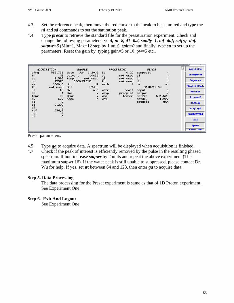
4.3 Set the reference peak, then move the red cursor to the peak to be saturated and type the nl and sd commands to set the saturation peak.
4.4 Type presat to retrieve the standard file for the presaturation experiment. Check and change the following parameters: ss=4, nt=8, d1=0.2, satdly=1, tof=dof; satfrq=dof. satpwr=6 (Min=1, Max=12 step by 1 unit), spin=0 and finally, type su to set up the parameters. Reset the gain by typing gain=5 or 10, pw=5 etc..
Presat parameters. 4.5 Type ga to acquire data. A spectrum will be displayed when acquisition is finished. 4.7 Check if the peak of interest is efficiently removed by the pulse in the resulting phased
spectrum. If not, increase satpwr by 2 units and repeat the above experiment (The maximum satpwr 16). If the water peak is still unable to suppressed, please contact Dr. Wu for help. If yes, set nt between 64 and 128, then enter ga to acquire data.
Step 5. Data Processing
The data processing for the Presat experiment is same as that of 1D Proton experiment. See Experiment One. Step 6. Exit And Logout
See Experiment One

NMR Course 2009 February 19, 2009 NMR Research Center
84
Plasma sample in 90% H2O + 10% D2O after the water peak suppressed.
Normal 1D proton spectrum of strychnine in CDCl3.
Same sample, but the peak at 6 ppm was suppressed.

NMR Course 2009 February 19, 2009 NMR Research Center
85
Experiment 9: Gradient Shimming Sample to be used: 2% H2O in dopped D2O
Step 1. Load your sample into the probe as usual. Type h1(‘d2o’) su to load the proton
experiment parameters. Ask an NMR staff person to help you tune the probe. Lock the machine and shim manually.
Step 2. Because of the huge water signal, the receiver will be overflowed if you start to acquire the data using the default value. To avoid the receiver overflow, do as follows: Type gain? to check the value of the gain. Change the gain value to a smaller value. The gain value could be set as small as 1. When acquiring the data. If you still get an “ADC overflow” error message after you set gain=1, then the pw value needs to be set to a smaller value until no “ADC overflow” message is shown. Save the spectrum and change to another experiment ( jexp2) to do gradient shimming.
Step 3. Turn on the Pulsed Gradient Driver module in the console (ask an NMR staff person for help if this is the first time you do this) Type pfgon=’nny’ Type gmapsys and press return. Click on Set Params > Gradient, Nucleus > Pfg H1 > Return > Go, dssh You may set the pw= “90 degree pulse” and p1= “180 degree pulse” these numbers are written on the log book of each instrument. After acquisition completes, there are two broad peaks displayed. If the peaks do not look like as following, then there is a problem. You may have to talk to our NMR center staff.
The click find gzwin, computer will find the gradient shim region.

NMR Course 2009 February 19, 2009 NMR Research Center
86
Then type gmapsys (Shimming size can be changed now by typing gzsize=7) Click on Shim Maps > Make Shimmap, then type a file name when prompted. (file is saved in directory /vnmrsys/gshimlb/shimmaps)
After you finish mapping, Click on Return > Display > Display Shimmaps (lines should be smooth in the shimmap)
Click on Return > Autoshim on Z The map rms err should be smaller than 1.00. Click on Set Shim

NMR Course 2009 February 19, 2009 NMR Research Center
87
Finishing: Type Pfgon=’nnn’ su Turn off the pfg module to standyby. Save the shim file svs(‘shim_021909’) Gradient Shim On VNMRS System: Same concept, but there is a little difference. Type gmapsys, a new window will come up. Click Acquire Trial Spectrum, That is same as Go dssh icon as above. If everything is OK, then click Make Gradient map, you may have to input the map name. After completed, then click auto gradient shim on Z. Save the new shim file.

NMR Course 2009 February 19, 2009 NMR Research Center
88
Experiment 10: COSY
Step 1. Login The Computer System See Experiment One
Step 2. Change Sample See Experiment One
Step 3. Lock And Shim The Magnet See Experiment One
Step 4. Setup Parameters And Run Experiment 4.1 Run a proton 1D spectrum by using proton standard parameters.(See Experiment One) 4.2 Set the two red cursors to define the desired sw (spectrum width); type movesw then ga,
Check the new spectrum and make sure no peak is fold in. Save this spectrum in case for later reference. Type COSY on the command line and type dg to show the parameters. Check the following parameters:
ss=4 dummy scans for COSY d1=2 delay; set to 2 seconds. fn1=2048 zero-fill the f1 dimension to 2K data points. tpwr=xx transmitter power of the 90o-pulse-width of proton channel: check the last
page of the log book. pw=xx.x 90o pulse width for proton: check the last page of the log book.
nt=8 minimum nt is 8 (16, 32). The larger the value, the better the spectrum. ni=128, 256 number of FIDs, (128, 256,512). The larger the value, the better.
Make sure sw = sw1 and fn = fn1 Type time to check the total experiment time. You can increase or decrease the value of nt or ni to fit your allotted time. Turn the spin off and type ga to start the experiment. After acquisition, save the data.
COSY parameters. Step 5. Data Processing and Spectrum Printing 5.1. Reload the data: Click on Main Menu and File , then highlight the file name and click on Load

NMR Course 2009 February 19, 2009 NMR Research Center
89
5.2. See detailed processing instruction in Experiment 17. Alternately, you could type wft2d foldt to autoprocess the data by using default processing parameters.
5.3. Adjust the vertical scale of the 2-D spectrum using the vs+20 and vs-20 button to eliminate the unnecessary background noise.
5.3 Type pcon page to print the 2-D spectrum. 5.4. To print 2-D spectrum with 1-D projection spectrum:
Click on Return, Size and Center buttons to place the spectrum in the middle of the screen.
5.5. Click on Proj, Hproj(max) and Plot buttons to display the horizontal projection1-D spectrum on the top of the 2-D spectrum. Use the MMB to adjust the vertical scale of the 1-D projection spectrum. Click on Vproj(max) and Plot buttons to display vertical projection 1-D spectrum on the left of the spectrum. Use the MMB to adjust the scale of the 1-D spectrum.
5.6. Type pcon page to print the 2-D spectrum with 1-D projection spectra. 5.7 To expend the area you are interested in:
Press and drag left mouse button to control a pair of the cursors (looks like a red-cross) and define the left and bottom edge of the spectrum. Use the right mouse button to control another pair of cursors to define the upper and right edge of the spectrum. Then click Expand to expand the spectrum.
Step 6. Exit And Logout See Experiment One
COSY Spectrum of Strychnine in CDCl3.

NMR Course 2009 February 19, 2009 NMR Research Center
90
Experiment 11: HETCOR Step 1. Login The Computer System
See Experiment One Step 2. Change Sample
See Experiment One Step 3. Lock And Shim The Magnet
See Experiment One Step 4. Setup Parameters And Run Experiment 4.1. In exp1, run a 1D proton spectrum by using standard parameters. After phasing and
setting reference, use the two red cursors to narrow the spectrum of interest by 1ppm upfield and 1ppm downfield. Type movesw to change the spectral width.
4.2. Type ga to run the 1D proton experiment with a modified sw. Phase the spectrum. 4.3. Type jexp2 to joint exp2. Run a 1D-carbon experiment. After phasing and setting the
reference, narrow the spectrum of interest using the two red cursors. Type movesw to change the sw. Remember you will not see these carbons without proton attached on the HETCOR. So set the correct sw will increase your spectrum quality!
4.4 Type ga to run the 1D carbon experiment with a new sw. Phase the spectrum. 4.5 Type hetcor to set up a standard HETCOR experiment. Remember: your proton
spectrum is in exp1. 4.6. Double-check the following two pairs of parameters (the correct values are listed on the
last page of the log book):
tpwr transmitter power for carbon pw 90° pulse for carbon
pp 90° pulse for proton decoupler channel pplvl proton pulse power for decoupler channel (pp and pplvl should be as same as the ones in DEPT experiment in Experiment 6) After entering correct values for the above parameters, check the following parameters:
ss=4 dummy scans sw= sw should equal to the sw value in exp2 for carbon domain
sw1= sw1 should equal to the sw value in exp1 for proton domain; dof= dof should equal the tof value in exp1 for proton; nt=n*16 acquisition scans of multiple of 16; ni=256 number of increments in 1st dimension; np=2048 number of points to record FID; d1=3 carbon relaxation time 4.7. Type time to check the experiment time. d1 can be adjusted to fill the allotted time. 4.8. Turn the spin off and do any needed minor shimming. Enter ga to acquire data. 4.9. Save the spectrum by typing svf(‘hetcor_mydata’)

NMR Course 2009 February 19, 2009 NMR Research Center
91
Step 5. Data Processing and Spectrum Printing 5.1. Recall the data “hetcor_mydata.fid” Click on Main Menu and File , then highlight the file name and click on Load 5.2. Type wft2da or follow the detailed processing method in experiment 17. 5.3 Click on Return, Size and Center buttons to place the spectrum in the middle of the
screen. 5.4. Adjust the vertical scale of the 2-D spectrum using the vs+20and vs-20 button to
eliminate the unnecessary background color.
5.4.1. Click on Proj, Hproj(max)and Plot buttons to display the horizontal projection 1-D spectrum on the top of the 2-D spectrum. Use the MMB to adjust the vertical scale of the 1-D projection spectrum.
5.6. Click on Vproj(max)and Plot buttons to display vertical projection 1-D spectrum on the left of the spectrum. Use the MMB to adjust the scale of the 1-D spectrum.
5.7. Type pcon page to print the 2-D spectrum with 1-D projection spectra. Step 6. Exit And Logout
See Experiment One
HETCOR Spectrum of strychnine in CDCl3.

NMR Course 2009 February 19, 2009 NMR Research Center
92
Experiment 12: 1D NOE Sample to be used: 10% Strychnine in CDCl3
Step 1. Login The Computer System
See Experiment One Step 2. Change Sample
See Experiment One Step 3. Lock And Shim The Magnet
See Experiment One Step 4. Setup Parameters And Run Experiment 4.1 Run a standard proton spectrum and save the file. 4.2 Put the cursor on the peak to be irradiated, then type nl sd to display the frequency,
shown as dof=xxx.xx on the top of the screen. Write down this first dof value (If the peak is a multiplet, put the cursor in the middle of the multiplet and type sd). Next, move the cursor to a no-peak region close to the peak to be irradiated, Type sd to display the second dof value. Make sure to record this value.
4.3 Type presat to load standard file for the presaturation experiment. Check and change the following parameters: ss=4, nt=8, gain=10, d1=2, satdly=1, satfrq=the first dof value written down. satpwr=2 (Min=1, Max=15 step by 1 unit), and type su. Finally, turn off the spin. Type ga to run a quick spectrum. Check if the irradiated peak has disappeared from the resulting spectrum. If not, repeatedly increase satpwr by 2 units and run the experiment again until the peak has disappeared.
4.4 Change the nt value to 128 or 256 and type ga to acquire data for the first spectrum. After the acquisition is finished, save the spectrum. 4.5.1 ONLY change the satfrq parameter to the second dof value recorded previously, then
type ga to obtain a second spectrum. Save this new spectrum. Step 5. Data Processing 5.1. Type jexp5 to go to Exp5 and load the first spectrum by the following procedure (you
must use Exp5 to do this operation): Click on Main Manu, File and highlight the first spectrum file, then click on load. Type lb=5 wft to show the spectrum.
5.2. Type jexp1 to go to Exp1. Load and process the second spectrum by the procedure as described in step 5.1.
5.3. Type spsub to subtract the second spectrum (in Exp1) from the first (in Exp5) and then type jexp5 and ds to show the resulting spectrum in Exp5. Type vp=50 to move the spectrum to the middle of the screen.
5.4. Plot the spectrum. Step 6. Exit And Logout
See Experiment One

NMR Course 2009 February 19, 2009 NMR Research Center
93
Experiment 13: 1D Carbon with Complete Fluorine Decoupling by Using Wave Function Generator
Sample to be used: 20% Perfluoro-2-methyl-2-pentene
Step 1. Login The Computer System (See Experiment One)
Step 2. Change Sample (See Experiment One) Step 3. Lock And Shim The Magnet (See Experiment One) Step 4. Setup Parameters And Run Experiment 4.1 type f19 to load standard fluorine parameters with CDCl3 as solvent. Run a F19
spectrum and save the file. 4.2 Find the value of tof by typing dg and record this value. tof is the center frequency of the
observe transmitter. 4.3 Find the transmitter frequencies for each peaks as follows: 4.3.1 Put the cursor on a peak and type movetof. Write down the new tof value after typing dg. 4.3.2 Load the original spectrum again and find the tof value for another peak as in step 4.3.1. 4.3.3 Repeat step 4.3.1 and 4.3.2 until all the frequency values for all peaks are recorded. 4.4 Calculate the offset value. 4.4.1 Subtract the transmitter frequency value of each peak recorded in step 4.3 from the tof
value of the spectrum recorded in step 4.2. Record these values. Remember, always subtract the frequency value of a peak from the tof value, so that
when the frequency of a peak is higher than the tof value, you get a positive offset value and when the frequency of a peak is lower than tof¸you get a negtive offset value.
4.5 Use Waveform generator to generate a shaped decoupling sequence: 4.5.1 Load the F19 spectrum and type wft 4.5.2 Click Pbox button on the menu bar
Click Het-dec Click Adiabatic and then type 300 after J in Hz on the top of the screen for C-F coupling. Click Options Click Offset and input the offset value of the first (leftmost) peak which should be decoupled. Click Bandwidth and input 4000------- the area will be decoupled. Click Return. Click WURST, three parameters will be displayed for the decoupling on the top.
4.5.3. Click Options and repeat the remaining steps in the step 4.5.2. until all the offset value are input. Click Close.
4.5.4. Click Name and give a file name for the shaped pulse. Click Close. The computer will ask you to Enter reference 90 degree pulse width (μse): (F19 90 degree pulse width) Enter reference power level: (power level when you measure the F19 90 degree)

NMR Course 2009 February 19, 2009 NMR Research Center
94
A shaped pulse will be displayed on the screen. Write down the following parameters: dres=x dmf=xxxxx Remember you shaped pulse file name.
4.5.5 Load the standard C13 experiment parameters by typing c13
Input following parameters: dres = x dmf = xxxxx dm = ‘nny’ dmm = ‘ccp’ dseq =’shaped pulse file name’ dof = the tof of F19 spectrum Type ga to acquire data.
Step 5. Data Processing See steps in Experiment Two. Step 6. Exit And Logout See Experiment One.
250 200 150 100 50 0 PPM
13C spectrum of (CF3)2CCFCF2CF3 in Acetone_D6 was acquired on INOVA600 without 19F decoupling.
2 0 0 1 8 0 1 6 0 1 4 0 1 2 0 1 0 0 8 0 6 0 4 0 P P M
Fully 19F decoupled 13C spectrum of (CF3)2CCFCF2CF3 acquired on INOVA600.

NMR Course 2009 February 19, 2009 NMR Research Center
95
Experiment 14: Variable Temperature Experiment (25 to 80 oC) Sample to be used: 10% Strychnine in CDCl3
Step 1. Login The Computer System
See Experiment One Step 2. Change Sample
See Experiment One Step 3. Lock And Shim The Magnet
See Experiment One Note: Double check your solvent boiling point or freezing point. If you need much higher
temperature or much lower temperature experiments, please let us know. We could help you. You may have to order a high pressure Liquid Nitrogen tank for Low temperature Experiments. The temperature range we have done on the Unity plus -120 oC – 120oC with a Broad Band Probe.
Step 4. Setup Parameters And Run Experiment 4.1 type h1(‘solvent’) to load standard proton parameters and run a normal 1D experiment. 4.2 For a single temperature:
type temp to open the temperature control box. Click on and drag the temperature bar to the desired temperature. Wait until the temperature reading on the remote display reaches the desired value, then for another 5 to 10 minutes to let the sample reach the equilibrium temperature. Shim the magnet again and type ga to start acquiring the data.
Step 5. Data Processing See Experiment One. Step 6. Terminated the variable temperature function and exit Click and drag the temperature control bar to 25oC. Wait until the temperature drops to
around 25oC, and click the temperature off button. Close the temperature control window. Exit and logout.

NMR Course 2009 February 19, 2009 NMR Research Center
96
Experiment 15: NOESY
The procedure for NOESY experiment is quite similar to COSY experiment (see experiment 9) Step 1 Insert your sample and tune the probe on proton channel. Step 2 Parameters Set-up and Run Experiment
Run a proton 1D spectrum by using proton standard parameters (See Experiment One) Using two cursors to define the sw (spectrum width) just wide enough to include all peaks and then type movesw and ga to run another proton experiment with new sw. Save the spectrum.
Step 3 Type NOESY to load NOESY parameters. Check the parameters:
pw= 90o pulse width of proton channel. tpwr= transmitter power of the proton channel for 90o pulse width d1=2 nt=16, or 32 ni=128 (or 256 or 512, depends on the machine time you have) Type time to check how long the experiment it will take and adjust the nt and ni to fit your time signed up. mix (mixing time)=0.3 The value is ranging from 0.1 to 0.6(ms) depends on the molecular size of your sample. To obtain best result, it is better to do a set of experiments with different mix value and chose a best spectrum. fn1=2048; fn=2048 np=2048 Turn off spin, Double check the non-spin shims. Type ga to start acquisition. After the acquisition, save the spectrum.
Step 4 Processing and Printing Reload your NOESY spectrum file by clicking on Main Menu and File , then highlight the file name and click on Load. Type wft2da to do automatic weighting and Fourier transformation or follow the procedure in Experiment 17 to process the data manually. For a good NOESY spectrum, you should deoxygenate your sample.
NMR Course 2009 February 19, 2009 NMR Research Center
97
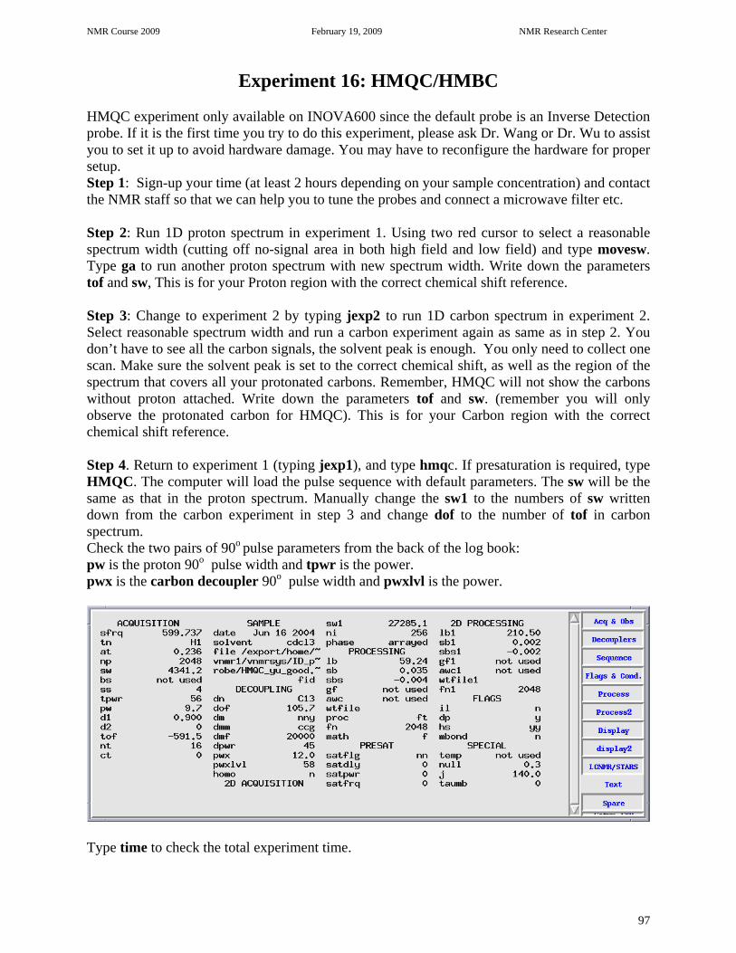
Experiment 16: HMQC/HMBC HMQC experiment only available on INOVA600 since the default probe is an Inverse Detection probe. If it is the first time you try to do this experiment, please ask Dr. Wang or Dr. Wu to assist you to set it up to avoid hardware damage. You may have to reconfigure the hardware for proper setup. Step 1: Sign-up your time (at least 2 hours depending on your sample concentration) and contact the NMR staff so that we can help you to tune the probes and connect a microwave filter etc. Step 2: Run 1D proton spectrum in experiment 1. Using two red cursor to select a reasonable spectrum width (cutting off no-signal area in both high field and low field) and type movesw. Type ga to run another proton spectrum with new spectrum width. Write down the parameters tof and sw, This is for your Proton region with the correct chemical shift reference. Step 3: Change to experiment 2 by typing jexp2 to run 1D carbon spectrum in experiment 2. Select reasonable spectrum width and run a carbon experiment again as same as in step 2. You don’t have to see all the carbon signals, the solvent peak is enough. You only need to collect one scan. Make sure the solvent peak is set to the correct chemical shift, as well as the region of the spectrum that covers all your protonated carbons. Remember, HMQC will not show the carbons without proton attached. Write down the parameters tof and sw. (remember you will only observe the protonated carbon for HMQC). This is for your Carbon region with the correct chemical shift reference. Step 4. Return to experiment 1 (typing jexp1), and type hmqc. If presaturation is required, type HMQC. The computer will load the pulse sequence with default parameters. The sw will be the same as that in the proton spectrum. Manually change the sw1 to the numbers of sw written down from the carbon experiment in step 3 and change dof to the number of tof in carbon spectrum. Check the two pairs of 90o pulse parameters from the back of the log book: pw is the proton 90o pulse width and tpwr is the power. pwx is the carbon decoupler 90o pulse width and pwxlvl is the power.
Type time to check the total experiment time.

NMR Course 2009 February 19, 2009 NMR Research Center
98
Finally type ga to start the experiment. After finish the experiment, save the data and report to the staff to help you reconnect the cable. Using the same procedure for HECTOR to process the HMQC data.
HMBC experiment is the same kind of experiment, the difference is you have to input the parameter of jnxh, that is the j coupling of three bond from proton to the carbon you are interested. The average number is 5 – 8 hz. Also you should double or triple of the nt scans, since HMBC is much less sensitive than the HMQC experiment. You may need little more samples.

NMR Course 2009 February 19, 2009 NMR Research Center
99
HMBC parameters:
HMBC spectrum of strychnine in CDCl3

NMR Course 2009 February 19, 2009 NMR Research Center
100
Experiment 17: 2D Data Processing Step 1. Load the data From the menu: Main File select the file you saved, then click Load. Step 2: Processing F2 dimension From the menu: Main Process Adj Weighting The following window will be displayed:
The top window is the spectrum that is the result after applying the window function and FT; the middle window is for the weighting function adjustment; the bottom window is the FID after applying the window function. From the menu, you could use lb (line broadening), sb (Sinebell weighting function), sbs (Sinebell squared weighting function), gf (Gaussian weighting function) and gfs Gaussian squared weighting function) functions by clicking the icon. Then move the mouse to the middle window to adjust the window function. The purpose of this operation is to make the peak shape as following:

NMR Course 2009 February 19, 2009 NMR Research Center
101
You could combine these window functions to change the shape of the peaks until you are satisfied with the spectrum. Then click return. If you acquired a phase sensitive 2D spectrum, there will be an icon “phase F2” on the menu, then you have to click phase F2. A 1D spectrum will be displayed. Phase it. If there is no “phase F2” icon, you acquired data is magnitude mode. You could click Transform F2. Computer will process the F2 dimension data. After it completes, a new window will be displayed.
If there is nothing in the window, change vs2d parameter, by typing vs2d=5000 or bigger. This will increase the display intensity level. Then click Redraw. The red lines are your data, and white area is zero filling.

NMR Course 2009 February 19, 2009 NMR Research Center
102
Step 3. Process the F1 dimension: There will be red line in the middle of the spectrum, use mouse to move the line on a blue line, then click Trace. Then click return Adj Weighting, A window will be displayed. Adjust the function as before.
Then click return F1 Transform. The computer will process the F1 dimension. The 2D spectrum will be displayed on the screen after few seconds. If it is a COSY spectrum, you could type foldt to get rid of the unsymmetrical noise. Don’t use foldt on NOESY!
COSY spectrum before foldt operation

NMR Course 2009 February 19, 2009 NMR Research Center
103
COSY spectrum after foldt operation Step 4. Display and Printing: On the menu, click return contour, to display the spectrum as contour mode. Click return size, to change the window size.

NMR Course 2009 February 19, 2009 NMR Research Center
104
Click project Hproj(max) to display 1D project spectrum. Click Vproj(max) to display 1D project spectrum on the side. You want to plot them with the 2D spectrum, you have to click plot after you click Hproj(max) or Vproj(max).
To add text by typing text(‘your_text’). Tp print the text by typing pltext. To print the spectrum, type pcon(18,1.4) page. The number 18 is the level, the 1.4 is spacing. If you have questions, please feel free to ask our service instructors.

NMR Course 2009 February 19, 2009 NMR Research Center
105
Experiment 18: 1D Carbon with Complete Fluorine Decoupling by Using Wave Function Generator (INOVA600 Only)
Sample to be used: 20% Perfluoro-2-methyl-2-pentene
Note: This is a special experiment that uses Wave Function Generator to construct a special decoupling sequence that is capable to decouple 19F with big spectral width. If you are interested, please contact us. Step 1. Login The Computer System
(See Experiment One) Step 2. Change Sample (See Experiment One) Step 3. Lock And Shim The Magnet (See Experiment One) Step 4. Setup Parameters And Run Experiment 4.1 type f19 to load standard fluorine parameters with CDCl3 as solvent. Run a 19F
spectrum and save the file. 4.2 Find the value of tof by typing dg and record this value. tof is the center frequency of the
observe transmitter. 4.5 Find the transmitter frequencies for each peaks as follows: 4.5.1 Put the cursor on a peak and type movetof. Write down the new tof value after typing dg. 4.5.2 Load the original spectrum again and find the tof value for another peak as in step 4.3.1. 4.5.3 Repeat step 4.3.1 and 4.3.2 until all the frequency values for all peaks are recorded. 4.6 Calculate the offset value. 4.4.1 Subtract the transmitter frequency value of each peak recorded in step 4.3 from the tof
value of the spectrum recorded in step 4.2. Record these values. Remember, always subtract the frequency value of a peak from the tof value, so that
when the frequency of a peak is higher than the tof value, you get a positive offset value and when the frequency of a peak is lower than tof¸you get a negtive offset value.
4.5 Use Waveform generator to generate a shaped decoupling sequence: 4.5.1 Load the F19 spectrum and type wft 4.5.2 Click Pbox button on the menu bar
Click Het-dec Click Adiabatic and then type 300 after J in Hz on the top of the screen for C-F coupling. Click Options Click Offset and input the offset value of the first (leftmost) peak which should be decoupled. Click Bandwidth and input 4000------- the area will be decoupled. Click Return. Click WURST, three parameters will be displayed for the decoupling on the top.
4.5.5. Click Options and repeat the remaining steps in the step 4.5.2. until all the offset value are input. Click Close.
4.5.6. Click Name and give a file name for the shaped pulse.

NMR Course 2009 February 19, 2009 NMR Research Center
106
Click Close. The computer will ask you to Enter reference 90 degree pulse width (μse): (F19 90 degree pulse width) Enter reference power level: (power level when you measure the F19 90 degree) A shaped pulse will be displayed on the screen. Write down the following parameters: dres=x dmf=xxxxx Remember you shaped pulse file name.
4.5.6 Load the standard C13 experiment parameters by typing c13
Input following parameters: dres = x dmf = xxxxx dn=F19 dm = ‘nny’ dmm = ‘ccp’ dseq =’shaped pulse file name’ dof = the tof of F19 spectrum Type ga to acquire data.
Step 5. Data Processing See steps in Experiment Two. Step 6. Exit And Logout See Experiment One.
250 200 150 100 50 0 PPM
13C spectrum of (CF3)2CCFCF2CF3 in Acetone_D6 was acquired on INOVA600 without 19F decoupling.
2 0 0 1 8 0 1 6 0 1 4 0 1 2 0 1 0 0 8 0 6 0 4 0 P P M
Fully 19F decoupled 13C spectrum of (CF3)2CCFCF2CF3 acquired on INOVA600.

NMR Course 2009 February 19, 2009 NMR Research Center
107
Experiment 19: Variable Temperature Experiment (25 to 80 oC)
Sample to be used: 10% Strychnine in CDCl3
Note: Double check your solvent boiling point or freezing point. If you need much higher temperature or much lower temperature experiments, please let us know. We could help you.
Step 1. Login The Computer System
See Experiment One Step 2. Change Sample
See Experiment One Step 3. Lock And Shim The Magnet
See Experiment One Step 4. Setup Parameters And Run Experiment 4.1 type h1(‘solvent’) to load standard proton parameters and run a normal 1D experiment. 4.3 For a single temperature:
type temp to open the temperature control box. Click on and drag the temperature bar to the desired temperature. Wait until the temperature reading on the remote display reaches the desired value, then for another 5 to 10 minutes to let the sample reach the equilibrium temperature. Shim the magnet again and type ga to start acquiring the data.
Step 5. Data Processing See Experiment One. Step 6. Terminated the variable temperature function and exit 6.1 Click and drag the temperature control bar to 25oC. Wait until the temperature drops to
around 25oC, and click the temperature off button. Close the temperature control window. Exit and logout.

NMR Course 2009 February 19, 2009 NMR Research Center
108
VNMRJ 1H Operating Instructions Note: All the commands you have learn from the VNMR (INOVA600, INOVA400) works on the VNMRJ.
Login Login to the system by entering your group’s user name and password. Starting vnmrj
1. Start vnmrj by single clicking the vnmrj spectrum icon at the top of the screen. 2. Choose to run a 1H experiment by dragging the proton icon on the left of the screen to
the black area or type h1(‘solvent’). The default solvent is CDCl3. Inserting your sample
1. Click spin off, and Click lock off and then Click eject to remove the standard from the magnet.
2. Replace the standard with your sample and click on insert. After the sample is proper
inserted, then click spin on. The spin rate is displayed at the bottom. 3. If you wish to use a solvent other than CDCl3, select which solvent you would like to use
with the drag‐down box on the following page. Click the Study tab. 4. If you would like to print a sample name/ID on your spectrum, insert this text into the
comment box (The text will print later by the command pap).
Single click this icon to start VNMRJ software.

NMR Course 2009 February 19, 2009 NMR Research Center
109
Shimming and locking your sample 1. If you are using a solvent other than CDCl3, click on the lock tab and change Z0, and
then Power, Gain, and Phase as necessary to lock your sample. The values can be adjusted with the left and right mouse buttons as in the case with the other instruments, or by typing in the desired value and pressing enter.
2. Shim your sample by first clicking on the shim tab, then by adjusting the Z1 Z2 and Z3 values. Use command “loadshim” to reload standard shim file for the standard sample.
Acquiring your 1 H spectrum 1. Check the current acquisition parameters by clicking on the process tag, then by typing
dg in the input box above the black box. 2. To change any parameters, click the acquire tag and make adjustments as necessary by
typing in the input box. Use the format “parameter = value” to make changes.
You sample ID and note should be type here
Use this to select solvent

NMR Course 2009 February 19, 2009 NMR Research Center
110
3. Alternatively, you may use the default parameters and simply change the number of scans by typing in the command input box (i.e., type nt = 16 for 16 scans).
4. Start the experiment by typing ga.
Processing your spectrum 1. After acquisition is complete, the spectrum should be displayed on the screen. 2. Apply the same commands as used on the other instruments to process the spectrum
(i.e., type wft vsadj aph in the input box for Fourier Transform, vertical scaling of peaks, and autophasing, respectively).
3. Displaying the scale: Note the set of processing icons to the left of the spectrum. Display the scale by clicking on the white ruler icon.
4. Expanding the spectrum: To expand the spectrum, select the top icon containing 2 red lines. Place the cursors where desired, then expand the region by choosing the zoom in/out (magnifying glass) icon. Use this icon to expand the spectrum and also to return to normal size.
5. Setting the solvent reference peak: As in the case with the other instruments, place the red cursor on your solvent peak, then type rl(x.xxp) in the input box to place the cursor directly on the peak and set the reference value (i.e., rl(7.27p) for CDCl3).
6. Integration: Click on the green integral icon, then take note of the two additional integration icons that appear just below it. Click the middle integration icon and use the mouse to cut the line, then return to the spectrum by typing ds in the input box. If necessary, you can also click on the top integral button or type cz to display the full integral.
7. Seting a peak integral reference value: To set a specific peak integration value, click on the process tab, then the cursors/integration sub tab. Place the cursor on the desired
NMR Course 2009 February 19, 2009 NMR Research Center
111
peak and type in the desired number of protons in the normalization value box. Save changes by clicking on the set integral value icon.
8. Set a precise spectrum width: To set a specific numerical range for your spectrum, use the same commands as used previously on other instruments (i.e., typing cr = 9.5p delta = 10p then clicking the expand icon will set the window from ‐0.5 to 9.5 ppm).
9. Setting the peak threshold: To choose the level of peaks for peak picking, press the icon labeled by the yellow threshold line and adjust the line accordingly.
10. Plotting and printing the spectrum To plot and print, type any combination of the following commands into the input box. Note that these are the same commands as the ones used for other instruments, but are listed here as a reminder.
pl : print spectrum pir: print integrals pscale: print scale pltext: print text label (from the comment box) pap: print acquisition parameters pll: print peak locations (ppm and Hertz) and peak height ppf: print peak frequencies above each peak page: eject page from the printer Saving the data
1. If you do not yet have a directory in your group’s folder, make a new directory by typing the command mkdir(‘directory_name’). Alternately, you can open your group’s folder (top left of the desktop) and create a new directory by selecting File Create folder. Command “pwd” to check the current directory.
2. To save a file in an existing directory, first choose the directory by typing cd(‘your_directory’). Next, save the file by typing svf(‘file_name’).
3. To retrieve your data later, find your file in your group’s folder on the desktop and drag it to the black processing window. Process as described previously.
Finishing the experiment 1. Eject your sample and replace with the standard sample. 2. If you used a solvent other than CDCl3, adjust the lock parameters back to the required
ones listed under the monitor. 3. Click on the loadshim icon at the top of the page, or type “loadshim” to reload the
standard shim file. 4. Manually shim the sample to reach the required lock level. 5. Exit the system by choosing File Exit vnmrj or by typing exit into the input box. 6. Logout by choosing Actions logout, then click OK.
VNMRJ 13C Operating Instructions Follow the VNMRJ 1H instructions to login to vnmrj and insert, shim, and lock your sample. Remember all the commands on the inova400 could be used on the VNMRS. Acquiring your 13C spectrum
1. Choose to run a 13C experiment by dragging the carbon icon on the left of the screen to the black area or type c13

NMR Course 2009 February 19, 2009 NMR Research Center
112
2. Check the current acquisition parameters by clicking on the process tag, then by typing dg in the input box above the black box.
3. To change any parameters, click the acquire tag and make adjustments as necessary by typing in the input box. Use the format “parameter = value” to make changes.
4. Alternatively, you may use the default parameters and simply change the number of scans by typing in the command input box (i.e., type nt = 16 for 16 scans).
5. After typing in the number of scans, type time to find out how long the experiment will take. If you run an excess number of scans and would like to stop early, type aa to abort the experiment.
6. Start the experiment by typing ga. Processing your spectrum
1. Apply the same commands as used on the other instruments to process the spectrum (i.e., type wft aph in the input box for Fourier Transform and autophasing, respectively).
2. Displaying the scale: As in the case for a 1H experiment, note the set of processing icons to the left of the spectrum. Display the scale by clicking on the white ruler icon.
3. Expanding the spectrum: To expand the spectrum, select the top icon containing 2 red lines. Place the cursors where desired, then expand the region by choosing the zoom in/out (magnifying glass) icon. Use this icon to expand the spectrum and also to return to normal size.
4. Setting the solvent reference peak: As in the case with the other instruments, place the red cursor on your solvent peak, then type rl(xx.xxp) in the input box to place the cursor directly on the peak and set the reference value (i.e., rl(77.23p) for CDCl3).
Follow the VNMRJ 1H instructions to plot and print the spectrum, save the data, and replace your sample with the standard sample. Before exiting the system, make sure to drag the proton icon to the black window then type su or type h1 to turn of the decoupler.
VNMRJ APT Operating Instructions Preparing for the APT experiment
1. Use the VNMR 1H and 13C instructions to shim and lock your sample. Change solvent settings as necessary. Drag the carbon icon to the black window and acquire a carbon spectrum using standard parameters.
2. Type wft aph to process the spectrum.
3. Use the toolbar to place the red cursors just to the left and right of the carbon peaks.
Type movesw to select this as the new range for the experiment. Remember all carbons, include solvent carbons, will show up on the APT spectrum.
4. Click on the Process and Text Output tabs. Type dg to load the updated parameters.
Record the values for sw and tof for use later in the experiment.

NMR Course 2009 February 19, 2009 NMR Research Center
113
Acquiring the APT spectrum
1. Drag the APT icon from the left of the screen to the black window (this will return the experiment to default parameters).
2. Using the values recorded previously in step 4, enter the new parameters for sw and tof
by typing sw = x and tof = x. Type dg and verify that the parameters are correct.
3. Enter the number of scans by typing nt = x, then type ga to start the experiment.
4. After the experiment is finished, type aptaph to automatically phase the peaks. If the phasing is still off, you can adjust manually by choosing the red circle icon on the toolbar and then adjusting with the left and right mouse buttons.
5. Set the solvent reference peak by typing rl(x.xxp).

NMR Course 2009 February 19, 2009 NMR Research Center
114
APT spectrum of Menthol in CDCl3. UP: CH2 and Cs and Down CH and CH3s.
6. Print the spectrum using standard processing commands. Finishing the Experiment
1. Remove your sample and replace with the standard sample, then turn on the spin and shim to the required lock level.
2. Drag the proton icon to the black window or type h1 to load standard parameters.
3. Exit vnmrj and log out.
Additional information: These instructions are very generalized. If you cannot obtain an acceptable APT spectrum, please see Dr. Wu for assistance, as additional parameters may need to be adjusted or the probe needs to be re‐tuned for your sample.
VNMRJ DEPT Operating Instructions Preparing for the DEPT experiment
1. Use the VNMR 1H and 13C instructions to shim and lock your sample. 2. Change solvent settings as necessary. Drag the carbon icon to the black window and
acquire a carbon spectrum using standard parameters. 3. Type wft aph to process the spectrum. Use the toolbar to place the red cursors just to
the left and right of the carbon peaks. Type movesw to choose this as your range for the experiment.
4. Click on the Process and Text Output tabs. Type dg to load the updated parameters. Record the values for sw and tof for use later in the experiment.
Acquiring the DEPT spectrum 1. Drag the DEPT icon from the left of the screen to the black window (this will return the experiment to default parameters). 2. Using the values recorded previously in step 4, enter the new parameters for sw and tof by typing sw = x and tof = x. Type dg to update the parameters. 3. Enter the number of scans by typing nt = x, then type ga to start the experiment. 4. After the experiment is finished, type autodept to automatically plot and print the DEPT spectrum.

NMR Course 2009 February 19, 2009 NMR Research Center
115
Finishing the Experiment 1. Remove your sample and replace with the standard sample, then turn on the spin and shim to the required lock level. 2. Drag the proton icon to the black window to load standard parameters. 3. Exit vnmrj and log out. Additional information: These instructions are very generalized. If you cannot obtain an acceptable DEPT spectrum, please see Dr. Wu for assistance, as additional parameters may need to be adjusted.
VNMRJ COSY Operating Instructions

NMR Course 2009 February 19, 2009 NMR Research Center
116
Preparing for the COSY experiment 1. Use the VNMR 1H instructions to shim and lock your sample. Change solvent settings as
necessary. Drag the proton icon to the black window and acquire the proton spectrum using standard parameters.
2. Process the 1H spectrum as listed in the instructions. Set the solvent reference peak, and save the file for later reference.
3. Type gain? in the command input box to determine the value to use for gain in the COSY experiment. For COSY or 2D experiments, you have set the gain, rather leave it as “autogain”.
4. Use the 1H spectrum to determine the spectral width for the COSY. Do this by placing the red cursor on both sides of the spectrum and typing movesw.
Acquiring the COSY spectrum 1. Click on the Homo 2D tab on the left of the screen. 2. Drag the COSY icon to the black window.
3. Type dg to view the current parameters. The parameters will be displayed after choosing the process tab (horizontal menu) and text output tab (vertical menu). 4. Change the gain value to the number used for the 1H experiment in the previous section. This can be done by typing gain = x in the command input box. 5. Change the number of scans by typing nt = x (where x = 16, 32, etc.). Note that the minimum is 4 scans, and a larger number of scans will lead to a better spectrum. 6. Change the number of FID’s by typing ni = x. Typically the desired values for x are 128, 256, 512, etc. It is best to start with at least ni = 256, and a larger value is better. 7. Check the parameters again as explained in step 3. sw=sw1, np=1024 or 2048, fn=2048 fn1=2048,Type time to see the length of the experiment. Adjust nt and ni to fit your allotted time.
NMR Course 2009 February 19, 2009 NMR Research Center
117
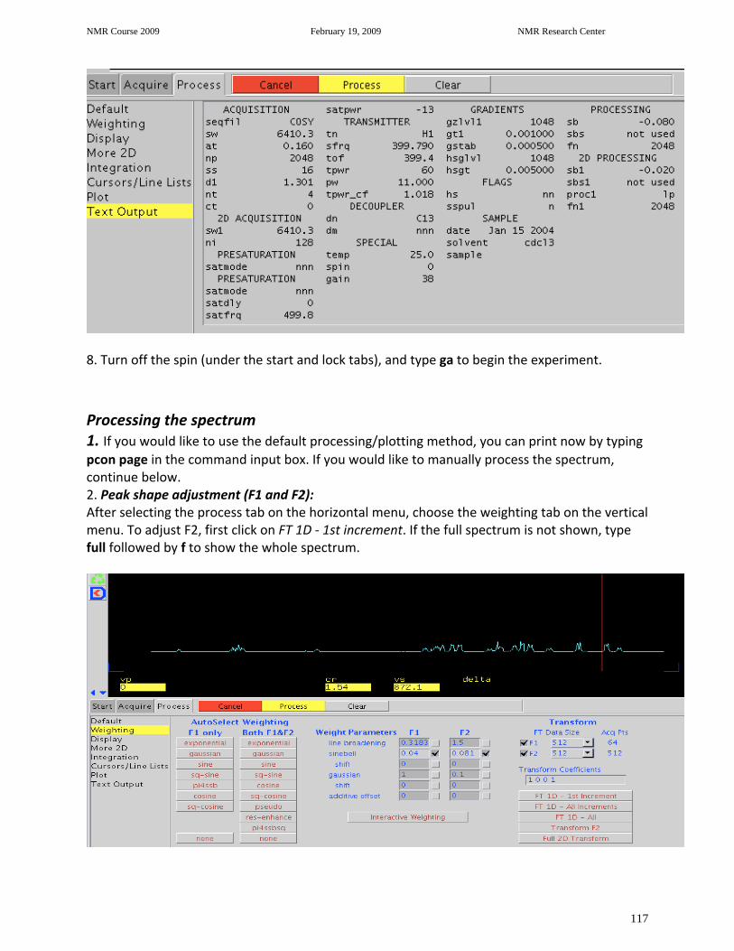
8. Turn off the spin (under the start and lock tabs), and type ga to begin the experiment. Processing the spectrum 1. If you would like to use the default processing/plotting method, you can print now by typing pcon page in the command input box. If you would like to manually process the spectrum, continue below. 2. Peak shape adjustment (F1 and F2): After selecting the process tab on the horizontal menu, choose the weighting tab on the vertical menu. To adjust F2, first click on FT 1D ‐ 1st increment. If the full spectrum is not shown, type full followed by f to show the whole spectrum.

NMR Course 2009 February 19, 2009 NMR Research Center
118
There are two options for adjusting the values for F2. You can simply input new values for F2 by entering numbers in the boxes under the weight parameters heading and F2 subheading, and then clicking the Transform F2 icon.
Alternately, you can manually adjust F2 by clicking on interactive weighting and adjusting the Gaussian curve with the left mouse button until the desired peak shape is obtained. When adjustment is finished, click the transform F2 icon.
To adjust F1, choose any single line of the spectrum using the red cursor lines, then click on interactive weighting and manually adjust the curve as described in the last step. When adjustment is finished, click the full 2D transform icon. 3. Eliminating peak noise: To remove excess unsymmetrical noise, type foldt in the command input box. 4. Setting the solvent reference peak: Note that this step is unnecessary if you have already set the reference peak in your 1H NMR experiment at the beginning of these instructions. However, if necessary, you may set this value by using the cursor and zoom

NMR Course 2009 February 19, 2009 NMR Research Center
119
(magnifying glass) icons to expand the area containing the solvent peak. Place the cursor on the desired peak and type in the command rl(x.xxp) to set the reference value. 5. Decreasing static noise: Click on the display tab on the vertical menu. Check to make sure that “none” is selected under Display Mode, then look for the 2D Contour Display heading. Select the static both +/‐ icon to decrease static noise.
6. Changing the screen position of the spectrum: look for the Screen Position heading. You may choose from the full, center, left, and right icons, depending on how you would like to plot your spectrum. Typically it is best to choose the center option since it will allow for easier plotting of the peaks and spectrum later. 7. Increasing/decreasing intensity of peaks: Adjust intensity of peaks by using the yellow bulb icons on the toolbar.

NMR Course 2009 February 19, 2009 NMR Research Center
120
8. Expanding regions of the spectrum: Choose the red cursor icon on the toolbar. Use the left and right mouse buttons to select the area to be expanded and click on the zoom icon to expand. Also use this icon to return to normal size. Plotting and printing the COSY spectrum 1. Select the Plot tab on the vertical menu.
2. Look for the Contour Plot heading, then click on the show icon next to the both subheading. Click on the plot icon just to the right to mount the vertical and horizontal contour. 3. To add your proton peaks to the spectrum, look for the Projection heading, then click on Horizontal and plot (icon directly to the right) to add the horizontal peaks. Add the vertical peaks in the same manner, by clicking on vertical and then plot. 4. To print, click on the plot page icon. Finishing the Experiment 1. Remove your sample and replace with the standard sample, then turn on the spin and shim to the required lock level. 2. Under the Standard 1D tab, drag the proton icon to the black window to load standard parameters. 3. Exit vnmrj and log out.

NMR Course 2009 February 19, 2009 NMR Research Center
121
Appendix A: Download Your Data from Host Computers to a PC
NMR Center has an internal network that is not connected to outside network. To access the NMR data on all NMR host computers, you have to use a PC to connect the internal network and download the data. There is a PC available in the NMR lab. Bring your own USB, or portable hard disk. Login if screen is locked: username: nmruser password: nmr4me or nmrforme Double Click on “Shortcut to Smart FTP” to open the Smart FTP window. Type the IP address of the host computer you want to download data from in ‘Address’ box.
IP addresses for each host computers: inova400: 170.140.188.70
inova600: 170.140.188.67 mercury300: 170.140.188.72 Type your group username in ‘Login’ box. Type the password of your group in ‘password’ box and press Enter. You maybe need to wait a couple of minutes to establish the connection. When you see the folders and files appear in the panels, the connection is established. Find your folders and files and drag them to the desktop (or you may want to create a temporary folder) on this computer. Copy the data to the media you like: USB flash drive (flash key), zip disk, floppy disk or burn your data on a CD. Delete your data and folders you created from this computer.

NMR Course 2009 February 19, 2009 NMR Research Center
122
Appendix B: When and how to use command su acqproc
su acqproc is a command to connect or disconnect the communication between Sun host computer and CPU board in the NMR console. There are several occasions users need to use it. When: The communication is lost. The computer seems not to respond to any command you typed in and you are not able to open the ‘acqi’ window. A word ‘inactive’ is usually shown after STATUS in the ACQUISTION STATUS window. How: Open the Console window by double click on the Console icon on the up-right corner of the screen (Sometimes it is hiding behind ACQUISTION STATUS window). Type su acqproc and press Return. A message “Starting ‘Expproc’ will show up. At same time “Word ‘inactive’ will change to ‘idle’ in the ACQUISION STATUS window. You should be able to operate the instrument again. When: The Lock button is missing in the ACQUISION window. It happens very often when you type h1, then immediately you clicked acqi. After you type h1, you should wait until “idle”, then click “acqi”. How: Open the Console window, type su acqproc and press Return to disconnect the communication. Type su acqproc and press Return again to establish the communication. If above operation doesn’t work, you should call Dr. Wu for help. Sometime you have to reset the console when he asks you to do so. The following pictures show the reset button on different console.
UNITY600 Plus Console RESET button position.
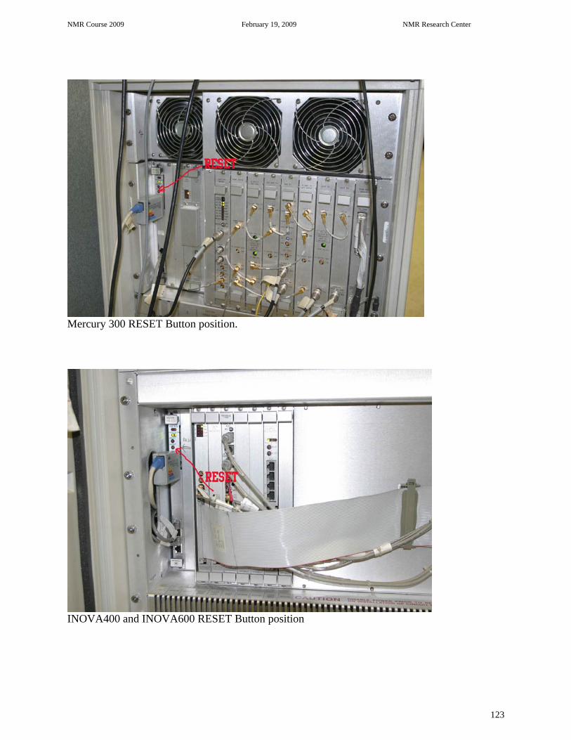
NMR Course 2009 February 19, 2009 NMR Research Center
123
Mercury 300 RESET Button position.
INOVA400 and INOVA600 RESET Button position

NMR Course 2009 February 19, 2009 NMR Research Center
124
Appendix C: Most Useful Commands and Parameters for VNMR and VNMRJ
aa—abort acquisition ai—absolute intensity mode alock=’n’ auto lock setting alfa----Delay time before acquisition aph—automatic phase correction at—acquisition time (sec) axis—scale units: axis=’h’ or axis=’p’ bc—baseline correction bs—block size cd—change directory: cd(‘/data/nmryao’) cexp—create experiment: cexp(7) cr—cursor value ct—completed transients (scans) cz—clear zeros (integral) d1—first delay (relaxation delay in seconds) d2—second delay in seconds da—display array (parameters) dc—drift correction dconi—display contours interactively delta—cursor difference df—display fid dfrq—decoupler frequency dg—display group of parameters dli—display integral list dll—display line list dlni—display normalized integral list dm—decoupler mode: dm=’nny’ dn—decoupler nucleus dof—decoupler offset dpcon—display plotted contours: dpcon(10,1.2) dpf—display peak frequencies dpir—display integral regions dpirn—display normalized integral regions dps—display pulse sequence dpwr—decoupler power dres—digital resolution ds—display spectrum dscale—display scale descale(-10) dssa—display stacked spectra dssh—display stacked spectra horizontally dtext---display text on the screen f—display full spectrum
foldt—symmetrize 2D data (cosy) fn—Fourier number (zerofill) fn1—Fourier number in 2nd dimension full—display spectrum in full window ga—acquire and process gain—receiver gain: gain=’n’ for autogain go—acquire spectrum ho—horizontal offset ins—integral normalization scale io—integral offset isadj—adjust integral scaling jexp—join experiment: jexp2 lb—line broadening lp—left phase movesw—move sweepwidth movetof—move tof mp—move parameters: mp(1,2) nl—nearest line nm—normalized mode np—number of points nt—number of transients (scans) pad—preacquisition delay page—send to plotter pap—plot all parameters pcon—plot contours: pcon(10,1.2) phase(180)—phase spectrum 180° pir—plot integral regions pirn—plot normalized integral regions pl—plot spectrum pll—print line list plot—plot everything plww—print spectra whitewashed ppa—plot partial parameters ppf—plot peak frequencies process—transform, phase, integrate spectrum spsub---Subtract current spectra from exp5. pscale—plot scale pw—pulse width pwd—present working directory ra—resume acquisition (stopped by sa) rl—reference line: rl(7.27p) rof2---Receiver gating time rp—right phase

NMR Course 2009 February 19, 2009 NMR Research Center
125
rt—retrieve FID rtp—retrieve parameters rts—retrieve shims sa—stop acquisition sc—start of chart (in mm) sc2—start of chart in 2nd dimension (in mm) sd—set decoupler frequency sda—add another decoupler value sfrq—spectrometer frequency sp—start of chart (in ppm) sp1—start of chart in 2nd dimension (in ppm) ss—steady state scans or dummy scans su—setup hardware parameters svf—save FID svs—save shims only svp—save parameters only sw—spectral width or sweep width temp—set temperature: temp=’n’ tn—transmitter nucleus tof—transmitter offset (middle of sweepwidth) tpwr—transmitter power text(‘your_ID\\date’) unlock—unlock a locked experiment: unlock(2) vo—vertical offset vp—vertical position vs—vertical scale vsadj—vertical scale adjust wc—width of chart (in mm) wc2—width of chart in 2nd dimension (in mm) wshim=’n’ start with auto shim wp—width of chart (in ppm) wp1—width of chart in 2nd dimension (in ppm) wft—weighted Fourier transform wft2d—transform 2D absolute value data wft2da—transform 2D phase-sensitive data wti—interactive weighting z—cut integral reset

Appendix D: Processing NMR data with NUTS on a PC
The data from Varian NMR instrument consist four individual files: fid, log procpar and text. The fid is the spectrum data. The log file contains the date of the spectrum acquired, The text file contain the note that you input by the command text(‘your_ID\\date’). And the procpar file contains all the acquisition parameters, including the shim data. In our NMR center, we have two off-line NMR data processing software: NUTS and MestReNova. For both software you have to purchase license, but you could download their trial version. http://www.acornnmr.com/ http://www.mestrec.com/ Also there are detailed operation manuals available for download. Following is an example to use NUTs process a spectrum from Varian instrument:
1. Open Nuts software by double click the icon:
2. Click ok to close the license window. Click File Import file select the file and open fid and click ok.

NMR Course 2009 February, 2009 Emory University
127
After the fid loaded:
You type lb:

NMR Course 2009 February, 2009 Emory University
128
If it is proton spectrum, set it to 0.2 hz, if it is a carbon spectrum set it to 2 hz. Then click ok Type bc em ft
Then type ap for auto phase.

NMR Course 2009 February, 2009 Emory University
129
Type zo and use cursor to select area you are interested:
The put the mouse into red area and click right mouse button.

NMR Course 2009 February, 2009 Emory University
130
Use the right bar to increase the peak height. Type id to integrate the spectrum. Click help for more information. You could print the spectrum at this point. You could print it as a PDF file. Type is to inset a spectrum above.
You could print the spectrum with the inset, integrals, and peak labels. Also you could save it a file that could use on the power point and Microsoft word. For further instruction, download the manual from their website.