Universita degli Studi di Genova

Short Thesis.

Neutrino astrophysics with theANTARES telescope.

Author:Vladimir Kulikovskiy

Supervisor:Dr. Marco Anghinolfi

External supervisor:Prof. Antoine Kouchner

January 16, 2013

1

The ANTARES underwater neutrino telescope was successfully build and operating inthe Mediterranean Sea. It has a capability to detect charged particles by the Cherenkov lightusing an array of the 875 photomultipliers. Ultra high energetic muon neutrinos producemuons with almost the same direction and energy as the origin neutrinos so their detectiongives information about the astrophysical source.

The main task for the telescope is the search for the cosmic source of the neutrinos. SNR,AGN, micro quasars are candidates for point like neutrino sources, the Galactic Center,the Galactic Plane, Fermi bubbles are candidates for extended sources

My PhD thesis consists to determine the minimum neutrino flux emitted by the two largeFermi bubbles structures measurable by the ANTARES telescope on the basis of the datacollected from 2008.

Contents

1. Introduction 32. High energy neutrino astrophysics 32.1. Cosmic rays 43. Possible sources of the high energy neutrinos from the gamma ray observations 53.1. GRB 63.2. Exotic high energy neutrino sources 64. Neutrino detection 64.1. Neutrino interaction 64.2. Cherenkov radiation 85. Atmospheric background 116. The ANTARES detector 126.1. General overview 126.2. Optical water properties 136.3. Optical background 146.4. PMT study 147. Data aquisition 167.1. Signal digitization 167.2. Data transmission 187.3. Data filtering and storage 187.4. Trigger 198. Detector calibration 208.1. Time calibration 208.2. Charge calibration 208.3. Position calibration 219. Monte Carlo simulations of the ANTARES detector 2310. Data quality using the Monte Carlo simulations 2311. Events reconstruction 2312. Track reconstruction 2313. Energy reconstruction 23

2

14. Search of the neutrino signal from the Fermi bubles 2314.1. Energy Spectrum and Cutoff 2514.2. Data set selection 2614.3. Off-zones for background estimation 2714.4. Validation of the off-zones choice and systematic error estimation 2914.5. Data/MC comparison 3014.6. MRF optimization 3314.7. Limits calculation 3414.8. Experimental results 3415. KM3net 3416. Conclusions 3417. Acknowledgments 34References 3418. Appendix A - Sparking run list 35

3

1. Introduction

Neutrinos are the lightest particles known and they can interact only by a weak force.These unique properties allow them to act as unique transmitter of information. In thespace they can go through interstellar matter, escape from the dense cores of the sources andgo without any deflections even through the strong magnetic fields. So instead of usingphotons like classical astronomers do, one could try to use neutrinos to look deeper inspace, look behind the nebulas, look inside the sources and etc. However these advantagesof neutrinos in respect to photons and hadrons bring a problem of their detection. Oneneeds megaton detector mass to try to detect astronomical sources.

But not only the possibility to find more sources is opens when one uses neutrinos in thetelescopes. Probably the most interesting result will be in understanding the accelerationof cosmic particles in space. There are several sources detected and there are gammasarriving from them with energies above TeVs. So far there are two conquering hypothesisfor the most discovered sources: leptonic model and hadronic. In the leptonic modelselectrons are accelerating first, in hadronic protons and heavier ions. Gammas can beproduced in both acceleration mechanisms (by the electrons via inverse Compton processor by decaying pions from the accelerated protons interacting with the matter surroundingthe source). Also decaying pions producing similar quantity of neutrinos but no neutrinosare expected from electrons. So neutrino detection from the source will be a smoking gunfor the hadronic model.

Neutrinos produce charged lepton (electron, muon, tau) and hardronic shower during aweakly interaction with matter. If one wants to do a telescope with an angular precisionof a degree or less, one needs to use muons that have the longest tracks in the medium(roughly 1 meter per 4 GeV). Muons can be detected by the Cherenkov light emittedin the medium due to the passage of charged particles which velocities are higher thenvelocity of light in the medium. Muon track is very less deviated from the neutrino oneat energies ¿ 10 GeV. So, for the neutrino astronomy one normally speaks about neutrinoenergies of several tens or even hundreds of GeVs. Also neutrino cross-section grows linearlywith the energy. Additionally, not only the previously described method can be used forthe neutrino detection. At ultra-high energies (above PeVs) one can try to use acousticand radio waves emitted during the neutrino interaction and hadronic shower propagationthrough the matter. two working detectors in the water: ANTARES in the Mediterraneansea and Baikal in the lake with the same name. There is an about 1 km3 project in ice atSouth Pole (IceCube) and there are two smaller working detectors in the water: ANTARESin the Mediterranean sea and BAIKAL in the lake with the same name.

2. High energy neutrino astrophysics

To start this chapter it is worth to mention a phrase from the J. Bahcall ”NeutrinoAstrophysics” book: ”The title is more of an expression of hope than a description of thebooks contents....the observational horizon of neutrino astrophysics may grow...perhapsin a time as short as one or two decades.” History shows that he was absolutely rightespecially in the low energy of the neutrinos: the detection of the solar neutrinos and super

4

nova neutrinos from the SN1986A become a classical part of the university books. Thereare also strong evidences that the high energy astrophysics is possible and may becometrue soon. First is that cosmic rays of E20eV were detected and second is that the highenergy gamma ray sources were observed.

2.1. Cosmic rays. The cosmic radiation incident at the top of the terrestrial atmosphereincludes all stable charged particles and nuclei with lifetimes of order 106 years or longer.Technically, primary cosmic rays are those particles accelerated at astrophysical sourcesand secondaries are those particles produced in interaction of the primaries with interstellargas. Thus electrons, protons and helium, as well as carbon, oxygen, iron, and other nucleisynthesized in stars, are primaries. Nuclei such as lithium, beryllium, and boron (whichare not abundant end-products of stellar nucleosynthesis) are secondaries. Antiprotons andpositrons are also in large part secondary. Whether a small fraction of these particles maybe primary is a question of current interest.

Cosmic ray spectrum measurements with air-shower detectors shown in fig. 1 demon-strates that protons and heavier nucleons with energies in the very broad range extendingto 1020eV arrive to the Earth. The above mentioned spectrum contains primary and sec-ondary particles. However only charged particles can be accelerated. The known stablecharged particles are protons and electrons. If first of them which can be not only protons,but ions in general are accelerated in a source, then due to interaction with the mattersurrounding the source neutrinos and gammas should be created via pion and kaon decays.The presence of the cosmic rays with an assumption that their primary particles werehadrons makes high energy neutrino detection theoretically possible. Instead if electronsare accelerated then only gammas maybe produced via inverse Compton process.

The question where the high energy cosmic rays are accelerated still remains on theinteresting unresolved problem in the astroparticle physics. The spectrum of the cosmicrays has a power law decrease with 2 changes on the power spectrum coefficient. Atseveral PeVs it changes from E−2.6 to a steeper one. This point was named a knee. It isbelieved among the most physicists that the most galactic sources accelerate particles tillthe energies around the knee so the cumulative distribution has this steepening. The nextchange in the power law spectrum can be explained that the cosmic rays coming below theknee have galactic origin while higher energies can not be gained by the galactic sourcesso the population of the cosmic rays above the ankle has an extragalactic origin.

For the source accelerating cosmic rays it could be extremely efficient to localize it onthe sky by detecting high energy particles and compare the observations with the opticaltelescopes. Air-shower detector don’t have a good angular resolution due to the fact thatthe primary charged particles itself are deflected in the magnetic fields (Earth’s and inter-stellar magnetic fields) so pointing accuracy is not possible for such instruments. Insteadrecently developed gamma ray detectors revealed several very interesting localized sourcesof the high energy radiation.

5

Figure 1. Cosmic ray spectrum as a function of E (energy-per-nucleus)from air shower measurements [2] ch. 26.5.

3. Possible sources of the high energy neutrinos from the gamma rayobservations

DESCRIBE the gamma ray detectors. Sources.Most of them are supernova remnants surrounded by the molecular clouds (SNR MC).

Super nova remnant RX J1713.7-3946 detected by H.E.S.S. has up to 30 TeV gamma raysin its spectrum (fig. 2). The idea of the explaining CR below the knee with shock accel-eration mechanisms in SNR becomes very popular last years even if recent fair theoreticalcalculations or Monte Carlo simulations still can not reach a PeV thresholds of energies.

A presence of the high energy gamma point sources such as previously mentioned RXJ1713.7-3946, other SNR MC such as Vela Jr and Vela X, and several other types ofthe sources such as Cygnus Region which is a star forming region is promising hope forthe neutrino detection from them or similar sources and opening an era of the neutrinotelescopes astronomy. The ideal case is that only hadrons are accelerated in these objects(pure hadronic model). In this case all the gamma rays are coming together with a similaramount of neutrinos. Their exact quantity may be calculated from the measured gammaray flux. For the RX J1713.7-3946 the expected number of the events per effective detector

6

Figure 2. RX J1713.7-3946 gamma ray measured spectrum together witha multicomponent prediction by the Zirakashvili & Aharonian [1].

area is Iµ+µ− = 2.4 ± 0.3 ± 0.5/km2 yr [1]. This shows that size of the detectors shouldbe on order of kilometers.

The center of our galaxy is an area of the active star formation. In this region SNexplosion rate is very high which makes it interesting for the neutrino detection. Anotherpossible extended source of the neutrino so-called Fermi bubbles will be explained in theproper section below. Both regions have significant high energy gamma emission.

3.1. GRB.

3.2. Exotic high energy neutrino sources. Talk about dark matter.

4. Neutrino detection

4.1. Neutrino interaction. Neutrinos interact only with a weak force. At high energiesthe deep inelastic scattering on the hadrons cross sections dominate over other possibleinteractions. There are two main channels: charged current (CC) via W± boson andneutral current (NC) via Z boson. Both are presented in fig. 3. In the first the high energylepton is produced. The cross section can be estimated by the equation [2]:

(1)dσ

dxdy(νN → l−X) =

G2Fxs

π[(d(x) + ....] + (1− y)2(u(x) + ...)]

and for antineutrinos:

(2)dσ

dxdy(νN → l+X) =

G2Fxs

π[(d(x) + ....] + (1− y)2(u(x) + ...)]

7

Figure 3. Neutral current interactions (left) in which neutrinos transfersand energy to hadron creating a cascade, charged current interactions (right)in which high energy lepton is created together with a hadronic cascade.

Figure 4. Neutrino (left) and anti-neutrino (righ) mean inelasticities <y >=< 1− E′/E > [5].

where x = Q2/(2Mν) is a fraction of the nucleon’s energy carrying by quark, ν = E − E′is the energy lost by the lepton in the nucleon rest frame and 1− y = E′/E. As it can beseen the cross section grows rapidly with the decrease of E − E′ and increase of E′/E sowhen the charged lepton brings out the incident neutrino energy. Including the momentumconservation law this means that the lepton has similar energy and the direction of theneutrino. The angle and energy change taken from the simulations described below arepresented in fig. 4 and 5.

Muons due to their bigger mass in respect to the electron and longer life time in re-spect to the tau have the longest tracks in the medium. Their energy losses in the highenergy region are proportional to their energy and starts at about 2MeV/cm at 1 GeV inwater (see fig. 6). Muons with TeV energies can pass through kilometers of water (fig. 8.Their passage causes Cherenkov light, e+e− pair production, Bremmstrahlung radiationand photonuclear interactions. The emitted light can be collected by the array of thephotomultipliers (PMTs) and the track reconstructed by the light time arrival.

8

Figure 5. Medians of the distributions of muon directions at the can forthe atmospheric and an E−2 neutrino flux [5].

Hadron products of the interaction create hadronic shower. Its size however is rathersmall in respect to the muon track which makes it difficult to detect with a sparse arrayof the PMTs. High energy electrons instead instead of muons have a very high probabilityto radiate bremsstrahlung photons after a few centimeters of water. This immediatelycreates an electromagnetic shower due to the γ → e+e− pair production. For the 10 TeVelectron, the shower length is only about 10 meters. For the tau due to its short life timeit is possible in principle to see double shower structure with a first shower coming fromthe interaction point of the incident neutrino and a second one due to the tau decay whichshould be separated by the tau decay length lτ = γctτ ≈ 50(Eτ/{textPeV )m.

Also it is possible in principle to detect a sound which is created by the expanding shockwave of the heated medium due to the neutrino interaction. This method seems to be verypromising for energies above 1020eV.

So far for the energy range of 100GeV − 1EeV the detection of the muons by theCherenkov radiation is the most precise and efficient method for the neutrino telescopes.

4.2. Cherenkov radiation. When a charged particle travels through a medium it po-larizes the atoms around its trajectory. These electric dipoles are symmetrically orientedaround the track when the particle is moving with a speed u smaller than the speed of light

9

Figure 6. Muon energy loss as a function of the energy due to ionization(a), the radiative processes (b) and total (c). [6]

c/n in the medium, where n is the index of refraction of the medium under consideration.If u ¿ c/n this symmetry is broken and dipole radiation is emitted, known as Cherenkovradiation. Cherenkov light is emitted at a fixed angle, creating a cone of light around theparticles track, and this fact makes it useful for reconstruction purposes. The Cherenkovangle can be calculated with the help of fig. ?? as follows. Consider a charged particletraveling with velocity ul = ? c emitting spherical waves of light along its trajectory.A spherical wave emitted at point A will reach point C at the same time as the chargedparticle arrives at point D. The cosine of the angle θc is given by:

(3) cosθc =AC

AD=tc/n

tβc=

1

βn

10

Figure 7. Muon maximum ranges in water [5].

Figure 8. A scheme of the Cherenkov radiation.

where for relativistic particles (β ≈ 1) and water as the propagation medium (n = 1.33)the value of this angle is about 41.2o. The spherical waves emitted at every point on thetrajectory collectively create a wavefront in the shape of a cone. The number of Cherenkovphotons emitted per unit track length x and wavelength ? is:

(4)d2N

dxdλ=

2παZ2

λ2(1− 1

β2n2)

11

Figure 9. Vertical muon intensity vs depth (1 km.w.e. = 105 g cm?2 ofstandard rock).[2]

where Z is the charge of the particle and ? the electromagnetic coupling constant. In theoptical part of the spectrum (350 nm ? 600 nm) which is of interest to us, this amountsto almost 200 emitted photons per cm. As the muon propagates through the medium,the Cerenkov light it produces is affected by absorption and scattering. The absorptionis characterized by the absorption length λabs, which is the average distance at which afraction of (1?1/e) of the photons is absorbed. Correspondingly, scattering is characterizedby the scattering length λs in the same way.

5. Atmospheric background

Cosmic rays interacting with an atmosphere produce hadronic showers containing mesons.Charged pions decay mostly to muons and neutrinos. Also there is a contribution fromkaons and other processes to the atmospheric muon and neutrino background. Rate of themuons from the overburden distance in rock is shown in fig. 9. Basically one can decreasethe muon background by 2 orders of magnitude going 2 km underwater. However even atthis depths the background is orders of magnitude bigger than the expected cosmic neu-trino signal. The Earth is not transparent to the muons so it is possible to use it as a shieldlooking for up-going signal from neutrinos. For the atmospheric neutrinos the rate almostindependent for up-going and down-going events with a difference coming only due to thegeomagnetic effect which changes flux of the cosmic rays. The flux of the atmospheric neu-trinos is also orders of magnitude bigger than the expected signal from the cosmic sourceshowever it decreases with the energy.

12

Figure 10. Depth contour plot near the ANTARES site.

6. The ANTARES detector

The ANTARES1 detector is a pilot project to demonstrate a possibility of the neutrinotelescope creation and stable operation during the years in the sea water on the big depth.The ANTARES detector is located near Toulon, France. The coordinates are 42o50′ N and6o10′ E. Its location makes it sensitive to a large part of the southern sky, including thegalactic center region. The detector is located at a depth of 2475m on the bottom of theMediterranean sea. The seabed in this place is quite flat (fig. ??) which is promising forthe further project extension.

6.1. General overview. The ANTARES detector consists of 12 vertical strings, each oneholding photomultiplier (PM) tubes for Cherenkov light detection. ANTARES comprises885 detector units, called optical modules (OM). The OM is a sphere containing the PMtube. A single storey consists of three such optical modules mounted on the optical moduleframes (OMF). Five storeys complete a single ANTARES sector. The optical modules pointdownwards at a 45? angle with respect to the vertical. The OMF is a mechanical structurewhich, in addition to the OMs, supports a titanium container holding the local controlmodule (LCM) and housing offshore electronics and processors. Five storeys togetherconstitute a sector which is an individual unit in terms of power and data transmission. Aline is a chain of 25 OMFs, i.e. 5 sectors, linked by an electro mechanical cable (EMC).The distance from storey-to-storey is 14.5 m and the first storey of each line is located 100m from the bottom of the sea. The reason for this is to leave enough space to allow for the

1Astronomy with a Neutrino Telescope and Abyss environmental RESearch

13

development of the Cherenkov cone from up-going particles. The inter-line spacing variesbetween 65-70 m.

Each line is anchored to the bottom of the sea with the bottom string socket (BSS)and a dead weight, and is held vertical by a buoy at the top. Every BSS contains astring control module (SCM), a string power module (SPM), calibration instruments andan acoustic release system. The acoustic release system allows for the recovery of thecomplete line. The SPM houses the power supplies for all sectors in a line while the SCMcontains electronics for slow control. The full con- figuration is octagonal as seen in figure2.9. In each sector, one LCM is the master LCM (MLCM) and its role is to handle datadistribution between all LCMs in the sector. A Dense Wavelength Division Multiplexer(DWDM) multiplexes the data signal from the 5 sectors onto one pair of optical fibers. Dataand power are transmitted between the lines and the shore via the 40 km long main electro-optical cable (MEOC) connected to the junction box (JB), and interconnecting link cables(ILC). Data arrives onshore in a PC farm located at the shore station (La Seyne sur Mer)where the ANTARES control room is located and data filtering is applied. Filtered data arecopied and stored remotely at a computer center in Lyon once a day. The instrumentationline (IL07) contains oceanographic sensors for measurements of environmental parameters.Line 12 and IL07 contain hydrophones which are used to test the feasibility of acousticneutrino detection. The IL07 and the top sector of Line 12 do not contain OMs.

Each OM consists of a pressure resistant glass sphere, 43 cm in diameter and 15 mmthickness. It contains a Hamamatsu R7081-20 hemispherical PM tube [Hama] with a diam-eter of 25cm and an effective sensitive area of 440cm2. Each PM tube has 14 amplificationstages and a nominal gain of 5 ? 107 at a high voltage of 1800 V.

The wavelength sensitivity range of the PM tubes is 300-600nm. The peak quantumefficiency (QE) is 23% at light wavelength of 350-450 nm. The charge resolution andtransit time spread (TTS) of the PM tubes are 40% and 1.5 ns respectively. The darkcount rate at the 0.25 photoelectron level is about 2 kHz. Each PM tube is surrounded bya ??metal cage to minimize the influence of the magnetic field of the Earth on its response.The high voltage is provided by an electronics board mounted on each PM tubes socket.Each OM also contains an LED calibration system explained in more detail in section 2.8.The PM tube is glued to the outer glass sphere by means of a transparent silicon rubbergel. The glass hemisphere behind the PMT is painted black and contains a penetratorwhich provides the power and data transmission connection to the outside.

6.2. Optical water properties. The performance of the detector depends on the opticalproperties of sea water, since light propagation in a medium is affected by absorption andscattering. Absorption reduces the amount of light that reaches the OMs while scatteringaffects the path of the photons and their arrival time on the OMs. Absorption and scatter-ing reduce the intensity of light as, I(x, ?) = I0(?)e?x/?abs(?)e?x/?s(?), (2.5.1) where x isthe optical path travelled by light and ?abs and ?s the absorption and scattering lengths,respectively. The absorption length as a function of the photon wavelength is shown infigure 2.10. Figure 2.11 illustrates the wavelength dependence of the scattering length.

14

Figure 11. Absorption (left) and scattering (right) lengths in water as afunction of the wavelength.

6.3. Optical background. There are two background contributions to photon detectionin sea water. The first one is the decay of the radioactive potassium isotope 40K,

40K ? 40Ca + e? + ??e (BR = 80.3%), (2.5.2)40K+e? ? 40Ar+?e +?(BR=10.7%). (2.5.3)The emitted electron energy in (2.5.2) can take values up to 1.33 MeV. A large fraction of

these electrons is above the Cerenkov threshold for light production. The photons emittedin the electron capture process (2.5.3) have an energy of 1460 keV. These pho- tons canlead to Compton scattering producing electrons above the Cerenkov threshold. The secondoptical background contribution comes from luminescence produced by var- ious organisms(bioluminescence). Bioluminescence can give rise to optical background up to several ordersof magnitude above the 40K contribution and these bursts can last for seconds. In figure2.12 the typical counting rate on a PM tube, i.e. hit frequency, as a function of time isillustrated.

The fraction of time during which the instantaneous background rate exceeds the baselinerate by at least 20% is called burst fraction. After monitoring deep sea cur- rents, it wasfound that the baseline component is correlated neither with the sea current nor with theburst frequency. However, long-term variations of the baseline were ob- served. A strongcorrelation between bioluminescence and sea current velocity has been observed, as shownin figure 2.13.

6.4. PMT study. Since the track reconstruction is based on the light arrival to the PMTit is necessary to know its TTS precisely to be used in the detector simulations later. Theperformed measurements are shown in fig. 12. The measure was performed with uniformillumination and with a point like beam toward the center of the photocathode. In both asignificant tail toward increasing arrival times can be observerd. According to [7], the tail,a bit larger for uniform illumination, might be ascribed to an additional inelastic scatteringof the photoelectron in the first dynode while the structure at 50 ns from the main peak isproduced by the elastic scattering. To this extent, assuming an uniform electric field of 60V/cm in the 14 cm distance of the first dynode from the photocathode, the 50 ns of thepeak roughly corresponds to the round trip of one electron from the first dynode to the

15

Figure 12. Dotted curve: point like illumination, continuous: uniform illumination;

photocathode and its way back. On the left side from the peak, the pre-pulses contributionmay be seen in the 10- 15 ns preceding the main pulse. As expected, the contribution ismore sensitive for the point like illumination which is directed toward the first dynode. Inthe same plot the dashed curve represents the Gaussian fit of the left side of the main peak.In the regular process the photon is converted to the electron and electron is multiplicatedon the dynode stack. Additionally several different situations may happen (fig. 13):

(1) After-pulses type 1: they appear in the first 80 ns after the main pulse and canbe produced by the luminous reaction on the dynodes while bombarded by theelectrons (fig 1b) or by the electrons escaped from the dynode in the direction tothe photocathode.

(2) After-pulses type 2: appear in the 80 ns -16 µs interval after the main pulse dueto the ionization of the phototube gas by the photoelectron. Different ions givedifferent contributions to the after-pulses time distribution (H+, He+ and heavyions CH+

4 , O+, N+2 , O+

2 , Ar+ and CO+2 ).

16

Figure 13. After(1a,1b,2) and late(3,4) pulses origin on a PMT.

(3) Late-pulses: the primary photoelectron suffers elastic or inelastic scattering in thefirst dynode without a secondary electrons emission, it turns towards the photocath-ode making a loop and only after it creates a cascade of electrons in the dynodes.The arrival time of the hit will be delayed.

(4) Pre-pulses: They appear due to the direct photoelectron emission on the dynodesfrom the photons which passed the photocathode without interaction. Due to this,the main pulse is arriving earlier and with smaller charge.

In fig. 14 afterpulses measurements are presented. One can see hits arriving after themain hit shortly after (in 10-40ns) or later (6-8µs). The total contributions of these af-terpulses 1.0% and 0.8% correspondingly. The late afterpulses (type 2) doesn’t affect thetrack reconstructions but simply increase the light background. Instead the fast afterpulsesshould be considered in the tests of the reconstruction algorithms.

7. Data aquisition

The role of the data acquisition (DAQ) system of ANTARES [Agui 07] is to convert theanalogue signal recorded by the PM tubes into a digital format that can be used for physicsanalyses. This includes preparing the detector for data taking, converting the analog PMtube signal and transporting, filtering and storing the data. In addition, the run settingsare archived. The DAQ system is a large network of processors, both on-shore and off-shore. The off-shore processors, integrated in custom made electronics, are connected tothe on-shore processors (standard PCs) by the electro-optical cable on the sea-bed. Aschematic view of the data acquisition system is shown in figure 2.15.

7.1. Signal digitization. A photon hitting the photo-cathode of a PM tube can producean electrical signal on the anode. The probability of an electron emission induced by a pho-ton is given by the quantum efficiency (QE) of the PM tube and is a function of the incidentphoton wavelength. The wavelength dependence of the quantum efficiency is shown in fig-ure 2.16. If the signal amplitude exceeds a certain voltage threshold, the signal is read-out

17

Figure 14. Time vs amplitude distribution of after-pulses type 1a&1b(top) or type 2( bottom).

18

and digitized by a custom application-specific integrated circuit, the Analogue Ring Sam-pler (ARS) [Fein 03]. The threshold is typically set to 0.3 photoelectrons to suppress the PMtubes dark current although this can vary among different PM tubes. The ARS can distin-guish between single photoelectron pulses (SPE) and more complex waveforms. receivingsignals. Four additional autonomous transponders are located around The criteria used todiscriminate the two classes are based on the amplitude of the the detector to increase theaccuracy of the global alignment. The depth of the BSS is determined with pressure sensorslocated at the BSS and during connec- gate. Onlytiocnhatorgtheeajnundctiiomneboinxf-woritmhatpiorenssiusrreesceonrsdoredonfothreSsPubEmeavrienet.sT.hIenscpaeseedsoofflargeorsignal, the time above threshold or the occurrence of multiple peaks within the time dou-ble pulses, the ARS can sample the PM tubes signal continuously with a tunable samplingfrequency of 150MHz up to 1GHz holding the analog information on 128 26 switched ca-pacitors. For physics data taking only SPE hits are used. A local clock is used by the ARSchips for the determination of the arrival time of the hit. The time resolution of the systemis better than 0.4ns. The charge of the analog signal is integrated and digitized by the ARSover a certain period of time using two 8-bit ADCs. The integration gate is typically set to40ns. After this period, the ARSs exhibit a dead time of around 200ns. Each PM tube isread by 2 ARSs operating in a token-ring scheme to minimize the effect of the dead time.The combined charge and time information is called a level 0 (L0) hit. All0.625ARS chipsin an LCM are read out by a Field Programmable Gate Array (FPGA) that arranges thehits produced 0.2 in a time window into a dataframe and stores it in a 64MB SynchronousDynamic Random Access Memory (SDRAM). The complete set of dataframes from allARSs 0.15 that correspond to the same time window is called a TimeSlice. A 20 MHzclock is used to provide a common time for all ARSs. It is synchr0o.1nized to the GPStime with an accuracy of 100 ?s. Through the optical fiber network, all local clocks on thedifferent storeys are synchronized with the master clock.

7.2. Data transmission. Each offshore CPU runs two programs controlling the datatransmission. DaqHar- ness handles the transfer of dataframes from the SDRAM to thecontrol room, while SCHarness handles the transfer of calibration and monitoring data(slow-control data). Transmission Control Protocol and Internet Protocol (TCP/IP) isused for communi- cation between the CPUs and for data transport. The LCMs in asector are connected to the MLCM in the same sector using an optical bidirectional 100Mb/s link. These links are merged using the Ethernet switch of the MLCM into a singleGb/s Ethernet link. Each string is connected with an electro-optical cable to the junctionbox which in turn is connected to the shore station with the 40 km long electro-opticalcable. The data are transported using dense wavelength division multiplexing technique(DWDM) [Seni 92]. Each sector and each string use a unique pair of wavelengths totransmit data along a single optical fibre to shore. The ControlHost package [Guri 95] isused for data transfer and communication among the processes in the DAQ system.

7.3. Data filtering and storage. All data, after the off-shore digitization, are trans-ported to shore without any further selection. The total data output of the detector inperiods of low bioluminescence (60-90KHz per PMT) is 0.3-0.5GB/s. Since most of it is

19

optical background it has to be filtered appropriately. Trigger algorithms are applied toidentify signals from particles traversing the detector by searching for space-time correla-tions in the data. Such physics events selected by the DataFilter program, are subsequentlywritten to disk with the program DataWriter. The DataFilter looks for a set of correlatedhits in the full detector in a window of about 4?sec. If an event is found, all hits during thistime window are stored. If ANTARES receives external GRB alerts all detector activity isrecorded for a few minutes. Data filtering or triggering is examined in more detail in thefollowing section.

7.4. Trigger. Physics data taking runs in ANTARES last for about three hours. Theaverage data rate of 625 MB/s for each detector string is reduced after filtering to ? 0.15MB/s for the whole detector. The duration of the run along with the start and end times, aswell as the trigger conditions are stored in the database. The majority of the data is opticalbackground due to potassium decays or bioluminescence. This overwhelming backgroundcan be reduced by a factor of 104 on the first filtering (triggering) stage [Jong 05a]. Such areduction is achieved by searching for hits within 20 ns in different PM tubes of the samestorey or single hits with an amplitude higher than 3 photo- electrons. Hits satisfying thesecriteria are called L1 hits. All other hits are called L0. This kind of selection is based onthe assumption that background hits should be uncorrelated and signal hits correlated.Two recorded hits on two different PM tubes are considered causally related if they satisfy,—t— ng d, (2.7.1) c where t is the time difference between hits, d is the distance betweenthe PM tubes and ng/c is the group velocity of light in water. In this time window anadditional 20ns is included to allow for uncertainties in the hit positions, time and lightscattering. Hits satisfying this condition constitute a cluster. If this cluster is large enough(typically 5 L1 hits) it is stored as a physics event. Physics events contain L1 hits thatfired the trigger as well as all L0 hits in 2.2 ?s from the first and last L1 hit. The reasonfor this is that this is the time it takes for a relativistic muon to travel approximately 650m i.e. traverse the detector. The hits contained in a physics event are illustrated in figure2.17. In addition to this first level selection, a second trigger level (e.g. 3N trigger) can beapplied. This includes a scan over a certain number of directions searching for coincidencescompatible with the Cerenkov light emission hypothesis. The expected time of a Cerenkovphoton is:

1?? ri??1ri ti=t0+c zi?tan? +u sin? , (2.7.2)CgC where t0 is simply an initial reference time on the muon track. The first term in

equation (2.7.2) describes the distance along the track up to the point where the Cerenkovphoton was emitted and the second term is the path from the point of photon emissionto the PM tube. This is illustrated in figure 2.18 for two illuminated PM tubes, where ti= (t1, t2), zi = (z1, z2) and ri = (r1, r2). Two hits are considered compatible with theCerenkov hypothesis if:

—t2?t1—z2?z1 +Rtan?C+20ns, (2.7.3) ccwhere we used the assumption that cos ?C = 1/ng . The 20 ns are added to account for

uncertainties on the time calibration, light scattering, and position of the storey. Additionalclusters can be formed by L1 hits. An example of this is the T3 trigger [Carr 07]. It accepts

20

more background hits, increasing the sensitivity in the low energy region with the drawbackof triggering on additional events that will be reconstructed badly i.e. it exhibits a higherefficiency at the expense of lower purity. A T3 cluster is defined as at least 2 L1 hits in3 consecutive storeys within a time window of 100 ns for adjacent and 200 ns for next toadjacent storeys.

8. Detector calibration

The precision of track and energy reconstruction is strongly dependent on the precisionof time, position and charge measurements. In this section, the calibration systems usedin ANTARES are discussed.

8.1. Time calibration. The time calibration in ANTARES [Agui 11] is performed usingpulses from LED and laser devices. A timing resolution on the recorded PM tube signalsof 1 ns is required to ensure the reliability of track and energy reconstruction. The internalclock calibration system measures the time offsets of each storey. It consists of the masterclock on-shore and a bi-directional optical communication system connected to all LCMs.The relative offset of each local clock can be measured by using a calibration signal sent bythe master clock and echoed back. The clock system assigns an absolute event time with aGPS master clock synchronization accuracy of 100 ?s. The optical beacon system [ANTA07] is used to calibrate the relative offsets between the PM tubes. Four blue (472 nm)LED beacons on storeys 2,9,15 and 21 of each detector line and two green (592nm) laserbeacons on the BSS of L7 and L8 are used for this purpose. The LED beacons are used forintra-line calibration purposes while the laser beacon, being much more powerful and ableto illuminate all the lines, is used for inter-line calibration. An initial set of time offsetsis determined in the laboratory prior to deployment. After deployment, these values maychange due to different factors such as temperature changes or stresses in the cables. Usingthe optical beacon system they are monitored periodically and readjusted as necessary. Asecond calibration system consisting of a blue (470 nm) LED inside each OM is used tomeasure time offsets between the PM tube photo-cathode and the read-out electronics.Internal LED and optical beacon measurements reveal less than 0.5 ns contribution ofthe electronics to the photon arrival time resolution. Thus, time resolution is dominatedby the transit time spread of the PM tubes which is about 1.5ns, and light scatteringand chromatic dispersion, which depends on the distance travelled by the photon. Thecalibration system just described provides a relative time calibration of better than 1 ns.

8.2. Charge calibration. The integrated charge of the PM tube signal has to be con-verted into the number of photoelectrons that created this pulse. The relation between thesignal amplitude and the number of photoelectrons is given by the transfer function of theAmplitude- to-Voltage Converter (AVC). This function is important for the measurementof the amplitude in the PM tube pulse, as well as for the correction of the time slewingof the PM tube signal i.e. the influence of the pulse amplitude and the pulse rise time onthe threshold-crossing time, illustrated in figure 2.19. The first step in charge calibrationisperformed on the test bench where the AVC transfer function is determined. In order

21

to do this, a pulse generator sends a direct signal to a pair of ARSs operating in a token-ring scheme. The pulse has a triangular shape with 4ns rise time and 14ns fall time. Thetransfer function and the dynamic range of the ADCs exhibit a linear behavior and canbe parametrized by the slope and intercept of the function. In addition to the test benchcalibration, regular in situ calibration runs have to be performed. These runs are usedto determine the pedestal value of the AVC channel, namely the offset AV C0pe valuecorresponding to zero photoelectrons, and the single photoelectron peak which is studiedby looking at minimum bias events, since light from potassium decays and bioluminescenceproduce in their majority single photons on the photocathode level. The charge spectrum,ignoring contributions from the second and higher photoelectron peaks, can be describedas [Jong 05b]:

?a(x?x ) ? (x?x1 )2 f(x) = Ae th + Be 2?2 , (2.8.1)where the first term corresponds to the contribution of the dark current. The second

term describes the single photoelectron peak as a gaussian with mean x1 and stan- darddeviation ?. The effects of the dynamic nonlinearity (DNL) of the AVC can be minimizedby considering the integral of the AVC spectrum: ??x 0 A B ??1(x?x1)2?? f(x?)dx? =e?a(x?xth) + ? , , (2.8.2)

where ? is the incomplete gamma function. A fit on the integrated spectrum leads to thedetermination of the single photoelectron peak. The same procedure is applied to identifythe pedestal region as shown in figure 2.20. The parametrization used is:

20 C ??1 (x?x0)2?? 0 ? 2 , 2?02 . (2.8.3)Charge measurements in AVC channels appear to be affected by time measurements

in the TVC channel. This is known as the cross-talk effect and can be attributed to across-talk of the capacitors inside the ARS pipeline. Plotting AVC against TVC values,as shown in figure 2.21, makes it possible to determine the correction to be applied. Afterapplying this correction most of the hits in a minimum bias event have a charge of onephotoelectron.

Due to the spread of the PM tube gain, the photoelectron peak is described by a gauss-ian function with mean AVC1pe. If the parameters of the gaussian distribution for onephotoelectron are ?1 and ?1, then for the coincidence of N photoelectrons the parameters ofthe gaussian distribution are, where AV C is the corrected AVC value taking into accountthe cross-talk effect. Light from potassium decay is also used to monitor how the detectorresponse evolves with time. A gain drop of the PM tubes is observed and is attributed tothe aging of the phototube. The charge pedestal value is almost constant in time, whilethe photoelectron peak drops by around 0.02 photoelectrons per month as can be seen infigure 2.22. The systematic error on charge calibration is estimated at around 30[Fehr 10;Bare 09].

8.3. Position calibration. Due to the flexible nature of the lines, water currents candisplace the position of the optical modules, especially on top storeys. As with timingand charge information, knowledge of the position of the optical modules is of high impor-tance for a precise event reconstruction. For this purpose a High Frequency Long Baseline(HFLBL) acoustic system is used to monitor the positions of five hydrophones along each

22

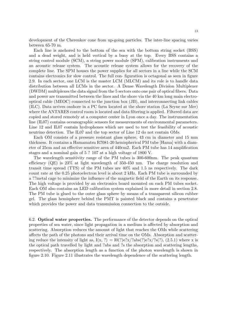
Figure 15. The horizontal displacement of the hydrophones on Line 11with respect to the BSS (0,0) for a period of six months. The East-Westtendency of the Line heading is due to the Ligurian current at the detectorsite. The top storeys of the line experience larger amounts of displace- mentdue to the water current. Image taken from [Brow 09].

line. The hy- drophones are mounted on storeys 1, 8, 14, 20 and 25. A transmitter-receiveris installed at the anchor of each line and some additional autonomous transponders areused. The emitters send high frequency acoustic signals in the 40-60 kHz range and thedistances are obtained by measurements of the travel times of the acoustic waves. Thedistances are used to triangulate the position of each receiver with respect to the emitterson the sea floor. Furthermore, a system of compasses and tiltmeters is used to measurethe orientation and inclination of each storey. The shape of each line is reconstructed byperforming a global ?2-fit based on a model of the mechanical behavior of the line underthe influence of the sea currents. The relative positions of each OM are calculated fromthis fit using the known geometry of each storey. In order to determine these positionsas accurately as possible, knowledge of the water current flow and the sound velocity insea water is used. These are measured using acoustic doppler current profilers (ADCP)for the water current flow, conductivity-temperature-depth (CTD) sensors to monitor thetemperature and salinity of the water and sound velocimeters to monitor the sound ve-locity in sea water. The relative positions of all the optical modules is monitored withan accuracy better than 20 cm [Ardi 09]. The horizontal movement of a line with respectto the BSS position is illustrated in fig. ??. The absolute positioning of each anchoreddetector component is calculated with an accuracy of about 1 m by acoustic triangulationfrom a surface ship equipped with differential GPS.

23

Figure 16. Fermi bubble γ-ray spectrum. The error bars are 1σ. Thesolid curve shows the best spectrum (E ∝ E−2.1

p ) the dotted curve showsthe steepest reasonable spectrum (Ep 2.3). For comparison the dashed curveis the spectrum expected were the bubbles suffused with protons having theE ∝ E−2.7

p distribution of the Galactic disk.

9. Monte Carlo simulations of the ANTARES detector

10. Data quality using the Monte Carlo simulations

11. Events reconstruction

12. Track reconstruction

13. Energy reconstruction

14. Search of the neutrino signal from the Fermi bubles

Recently the Fermi-LAT experiment has revealed two large spherical structures centeredin our Galactic Centre and perpendicular to the galactic plane, the so called Fermi-Bubbles.These structures [3] are characterized by gamma emission with an hard and uniform spec-trum (fig. 16) and a relatively constant intensity all over the space.

From the fig. 16. it is clearly seen that gamma flux is compatible with the flat E−2 dis-tribution at level of 3×10−7E2GeV cm−2 s−1sr−1. This spectrum can be hardly explainedby the Inverse Compton process of the highly relativistic cosmic ray electrons requiring

24

Figure 17. Figure 2 Visibility of the Fermi bubbles of the ANTARESdetector (left) and IceCube (right)

Figure 18. Shape of the Fermi bubbles region from [3] (green) and ap-proximated for this analysis (black)

very specific acceleration features. In other hand a population of relic cosmic ray protonsand heavier ions would naturally explain all the features of the Fermi bubbles structure [4].

In this scenario, the presence of high energetic hadrons makes the Fermi bubbles apromising neutrino source for the ANTARES detector. The ANTARES detector, locatedin the northern hemisphere, has an excellent visibility of the Galactic Center and thereforeof the Fermi bubble. So the advantage of this experiment in respect to IceCube, locatedin the South Pole, is that the visibility of the Fermi-Bubble is almost 100% (see fig. 17).

In this analysis the shape of the Fermi bubbles has been approximated as shown infig. 18.

25

Figure 19. Predicted number of neutrino events as a function of the neu-trino energy in the case of atmospheric neutrinos and neutrinos from theFermi-Bubbles for different energy cutoffs. Number of the events is in arbi-trary units (which correspond to about 4 years of data with precut describedbelow).

14.1. Energy Spectrum and Cutoff. For the known gamma ray emission with an almostflat E−2 distribution it is easy to estimate a neutrino flux assuming pure hadronic model.According to [?] (formula 34 + fig.3 at Γ = 2) there is the following relation between theneutrino flux and the gamma flux in this case:

(5) Φν ≈ 1/2.5Φγ

So, according to fig. 16:

(6) E2dΦν/dE ≈ 1.2× 10−7E2GeV cm−2 s−1sr−1

The Energy cutoff may be obtained from the proton cutoff:

(7) Xν ≈ Xp/20

Suggested cutoffs from [4] are from 1PeV till 10PeV in the most promising case whichwill correspond to cutoffs in neutrino spectrum from 50TeV to 500TeV correspondingly.Fig. 19 shows the comparison between the predicted number of detected neutrino eventsin the ANTARES detector in case of the atmospheric neutrino flux (Bartol flux) and theFermi bubbles flux considering different energy cutoffs.

26

Figure 20. Ratio of the events with λ > −6.5 in one data run to MC vstime of the run start with the exponential fit. Red dots correspond to theselection | log2(ratio/fit)| < 3σ.

14.2. Data set selection. For all the analysis following data and MC productions wereused:

• Data production: 2012-04 converted to AntDST v3r3 by Fabian• MC muons v2 RBR by Colas for muons• MC neutrinos v2.2 RBR by Katya and Luigi (genhen bug fixed)

First selection of the runs was done with following criteria:

• QB≥ 1• no words ”SCAN”, ”PRELIM”, or ”prelim” (we still don’t have an analysis to give

this runs back to normal)• no words ”half” & ”over” - to exclude gain/2, gain/4, gain/8 (this runs are quite

different and should be analyzed separately• the known sparking runs were excluded from the following analysis (see Appendix

A)

For the selected runs ratio of number of events in data to MC muons selecting triggers3N, T3, T2 and TQ which are reconstructed with Aafit with λ > −6.5 is presented infig. ?? together with exponential fit. From the fit it seems that the ratio data/MC isdecreasing over time. There is about 6% efficiency loss a year with unknown reason whichmay be an OM detection efficiency degradation (biofouling, PMT efficiency loss due to thephotocathode degradation o etc).

For the following analysis it was decided to remove the runs whose ratio of data/MCstays away from the fit. Basically the | log2(ratio/fit) for each run was calculated. Thedistribution was fitted then with a Gaussian as present in fig. 22. It was decided to keepruns with | log2(ratio/fit)| < 3σ.

At the end 8193 runs were selected starting from March 2008 till December 2011. Alsofor these runs grouped by 4 calendar weeks a ratio of number of neutrinos (up-going events)

27

Figure 21. Ratio of the events with λ > −6.5 in one data run to MC distribution.

Figure 22. Ratio data/MC of the up-going events with λ > −5.1 in off-zones grouped by 4 calendar weeks.

in data to MC in off-zones with λ > −5.1 was calculated (the choice of the cut and off-zones selection will be explained later). Similar decrease may be seen in the ratio in fig. ??although the fit values are consistent with no decrease hypothesis on 2σ level.

14.3. Off-zones for background estimation. As it is seen from the fig. 19 the presenceof the background of the atmospheric muons makes the signal search a difficult issue. Thecorrect background treatment is vital for this analysis.

28

Figure 23. Visibility of the ANTARES detector in Galactic coordinates.Fermi bubbles area is seen in the center together with 3 off zones aroundthe maximum of the visibility.

The uncertainty on the fluxes of the atmospheric neutrinos during the last years remainsmore than 20% due to the lack of new measurements of the cosmic ray fluxes and interac-tions of them with the light atoms in the atmosphere. This and other imperfections of thesimulations makes inefficient data/MC comparison for revealing a possible signal. Instead,the so-called off-zone method which is based on the background estimation from the dataexists and seems to be promising in this case. The main idea of this method is to comparesignal measured in the Fermi bubbles area (on-zone) with a background estimated fromthe data itself in the area chosen outside (off-zone). The estimated background in bothzones (on-zone and off-zone) should have the same properties.

The proposed off-zone was selected in a way that it has the same size and shape as theon-zone and it follows it in the local coordinates of the detector with some fixed delayin time. This allows to have the same expected number of background events, as theirnumber is proportional to the efficiency of the detector, which is a function of the localcoordinates only, and it slightly varies in time. The advantage is also that in this case theoff-zone is fixed in the sky. Also one can select at maximum 3 off-zones, which reducesthe background uncertainty. The Fermi bubbles area and 3 off-zones are showed in fig. 23together with a visibility of the detector. One can see that visibility of the on-zone andthe 3 off-zones is the same.

For the preliminary analysis it has been agreed with the referees (M. Spurio and C.Riviere) that all data taking period can be used freely to optimize cuts and to do data/MCcomparison with the restriction to look only at the events coming from the off-zones.

29

Figure 24. Difference between number of MC atmospheric neutrino eventsin on-zone and mean of off-zones divided by the last as a function of themean number of events (8). A gray band shows a statistical uncertainty.

14.4. Validation of the off-zones choice and systematic error estimation. Theconsistency of the number of events was checked with the following method. Arbitrary cuton lambda and energy from ANN energy estimator was chosen and number of events in3 zones calculated. As a first test MC neutrinos were used (the final cut removes almostall muons as it will be shown later). For each possible cuts combination in λ and energy(λ > (−6... − 4.9) and E > (102...106)[GeV]) a following ratio of events in the zones wascalculated:

(8) R =|Non-zone− < Noff-zone > |

< Noff-zone >× 100%

where Non-zone is the number of events in on-zones and < Noff-zone > is the average of eventsin off-zones. This ratio was plotted versus number of events < Noff-zone > in fig. 24. Thedifference between the ratio and corresponding statistical error indicates the systematicerror which can be estimated on order of 1% from the plot.

30

Figure 25. Difference between number of data events in off-zone 1 and off-zone 2 (black) divided by mean number of events in 3 off-zones as a functionof the mean number of events. The same distributions are presented for off-zones 2 and 3 (red), off-zones 3 and 1 (blue). A gray band shows meanstatistical error.

Also to do a check with a real data a similar plot for off-zones only is done. In this casethere are three different ratios:

(9) R =|N i

off-zones −Noff-zones|j |< Noff-zones >

× 100%, i 6= j, i, j = 1..3

As in this case the uncertainty is expected to be slightly bigger due to the differencesbetween (8) and (9)one can conclude that systematic error of 1% order is confirmed on thedata as well.

14.5. Data/MC comparison. Although Monte-Carlo simulations are not used for thediscovery claim it is needed for the cuts optimization and cosmic neutrino flux estimationafter measurement is done. A comparison of the data/MC is done for the following precut:

• λ > −6• β < 1o

• nhits ¿ 10• tχ2 < bχ2

31

Figure 26. λ distribution with data (black), sum of MC (red), νatmMC(blue), µMC (yellow), ν from Fermi bubbles with cutoff 100TeV MC (green)for the precut.

• events reconstructed as up-going• arriving from 3 off-zones

Where β is the estimated reconstructed direction error and 1o was chosen to be surethat probable signal events don’t penetrate to the off-zone and vice versa. The choice ofthe cut tχ2 < bχ2 is needed to get rid of the remaining sparking events. This cut is veryefficient for this task as it was seen that it remains only 3% of the sparking events (thetests were done on the run 38347). Also it improves a lot the data/MC comparison in allenergy range and what is more important - in the range of the high energies (3 events fromthe 10 with the highest estimated energy seemed suspicious on the event display and wereidentified as sparking with this cut). Cut on the up-going events is needed to reject thebackground from the atmospheric muons. The proposed cut on the events below horizonto decrease muon background seems to be redundant as the cut beta < 1o plus up-goingevents selection with later optimization on λ is sufficient to consider the muon backgroundas negligible.

The λ distribution in fig. 26 shows that at λ -5.25 there is a change of the main back-ground component: for λ < −5.3 there are more muons and for λ > −5.2 there are moreneutrinos. If one fits both areas a 13% lack of of muons and 27% excess of neutrinos is

32

Figure 27. EANN distribution with data (black), sum of MC (red),νatmMC (blue), µMC (yellow), ν from Fermi bubbles with cutoff 100TeVMC (green) for the precut.

seen in MC. Both effects can be a cumulative effect of the primary atmospheric particlefluxes arriving to the detector plus different efficiency of the detector in the MC.

The comparison of the ANN energy estimator for neutrinos is shown in fig. 27 for precutwith a stricter cut λ > −5.1 to cut atmospheric muons. Also the cumulative distributionintegrating from highest λ is shown in fig.28.

It maybe seen that there is slightly higher energies for data events than for MC ones.This problem produces an additional increase of the data/MC ratio in a high energy regionwhich is actually more correct to interpret as a ”shift” in a logarithmic energy scale. Inorder to tune MC the scale of 22% CHECK was applied first and then a fit of the shiftwith a step of the histogram bin size (log10E = 0.1) to find the best energy rescale. At theend the value of the shift log10E = 0.2 was used in further analysis together with the scaleof 22%.

It is known that there is a 30% systematic uncertainty on the atmospheric neutrino fluxso needed 22% normalization may be due the systematic uncertainty. Instead the lowerreconstructed energy of the events in MC may be explained by the uncertainties in thewater properties and probably by the PMT angular acceptance (however the later should

33

Figure 28. EANN cumulative distribution of the events integrating fromhighest λ with data (black), sum of MC (red), νatmMC (blue), µMC (yel-low), ν from Fermi bubbles with cutoff 100TeV MC (green) for the precut.

have minor impact on the up-going neutrinos). The proper tests are foreseen with ClancyJames to prove this.

14.6. MRF optimization. Analysis was optimized to have minimum of the MRF (modelrejection factor) which sets best limits in case of the no-discovery. The standard Feld-man&Cousins approach was used to calculated the average upper limit. It is known thatthis method gives slightly lower limits than the proper calculation including the systematicerror (as it will be discussed below) however as systematic error is low the current approachshould be acceptable for the cuts optimization.

The chosen cut parameters were λ and energy. The estimated energy is needed to rejectthe atmospheric neutrino background while λ is needed mostly to cut atmospheric muons.Two different optimizations were done: in first signal and background were taken fromMC (taking the average from the on-zone + off-zones to increase the statistics) and in thesecond the average of the data events in off-zones was used for the background togetherwith the same signal as in the first method.

The table 29 below shows the cuts minimizing MRF for different energy cut offs. DE-SCRIPTION OF THE TABLE. It is noticeable that for the all cut choices the expectedbackground in MC is in the very good correspondence with the average number of data

34

Figure 29. MRF optimization.

events in the off-zones which demonstrates the sanity of the scale and shift of the MCenergy distribution as explained in the previous section.

As it seen from the table cut optimized for the 100 TeV applies to the case with adifferent cutoff the obtained MRF is comparable with the case when the optimization isdone for the appropriate cutoff. This shows that only one cutoff may be used for the cutoptimization which simplifies the analysis.

14.7. Limits calculation. After unblinding request the selected cut λ > XX, E > Y Ywill be applied on the data. From the 3 off-zones one measures Nbg events and fromthe Fermi bubbles zone Nobs. Limits (upper/lower) on the signal expressed as number ofevents are calculated with Bayesian approach for 90% C.L. using the likelihoodciteLimits:(10)L(Nobs,Nbg|s, b, tau, sigma) = Poisson(Nobs|s+ b)Poisson(Nbg|τ ∗ b)Gaussian(τ |3, σ)

In case lower limits are not 0 it is possible to express the discovery in sigmas assuminga Gaussian distribution of Gaussian(NsignNbg/3, stat+ systerror).

The limits (Slower, Supper) calculated as number of events may be expressed as a fluxusing MC. In order to do so Nsignal MC for A = 1.2×10−7E2GeV cm−2 s−1sr−1 is calculatedapplying cuts on the cosmic neutrino events in MC.

(11) Φlimit = Stextupper/NtextsignalMC ∗AThis simple calculation is valid as the data/MC agreement after the tuning is very good.

To account for the 30% uncertainty in the atmospheric neutrino fluxes. NtextsignalMC

should be varied from +30% to -30% and the worst limits should be presented as the finalresult.

For the chosen cutl number of the observed background events in 3 off-zones is XXX.For this number upper and lower limits are presented in fig. 30.

14.8. Experimental results.

15. KM3net

16. Conclusions

17. Acknowledgments

References

[1] F.Vissani, F.Aharonian, ”Galactic Sources of High-Energy Neutrinos: Highlights”, [arXiv:1112.3911v1[astro-ph.HE] 16 Dec 2011]

[2] J. Beringer et al.(PDG), PR D86, 010001 (2012) (http://pdg.lbl.gov)[3] M. Su, T. Slatyer, D. Finkbeiner, Giant Gamma-ray Bubbles from Fermi-LAT: AGN Activity or

Bipolar Galactic Wind?, arXiv:1005.5480v3 [astro-ph.HE].[4] R.Crocker, F.Aharonian The Fermi Bubbles: Giant, Multi-Billion-Year-Old Reservoirs of Galactic

Center Cosmic Rays, arXiv:1008.2658v4 [astro-ph.GA] 14 Feb 201

35

Figure 30. Limits for Nbg = XXX calculated using the Bayesian approachwith a flat signal prior and likelihood Poisson(Nobs — s + b) Poisson(Nbg —tau * b) Gaussian(tau — 3, sigma). Upper limits are drawn with continuousline, lower - dotted.

[5] D. Bailey, ”Monte Carlo tools and analysis methods for understanding the ANTARES experiment andpredicting its sensitivity to Dark Matter”, PhD thesis work, Trinity Term, 2002.

[6] S.I. Klimushin, E.V. Bugaev, and I.A. Sokalski. ”Precise parametrizations of muon energy losses inwater”. 2001, Contribution to the 27th ICRC, Hamburg.

[7] B.K.Lubsandorzhiev et al. Nucl.Instrum.Meth. A567 (2006) 12-16.

18. Appendix A - Sparking run list

30658 31309 33608 33610 34663 34665 35467 36600 36666 36670 36689 38347 38348 3834938351 38352 38353 38355 38357 38482 39192 41668 41671 42507 42509 42511 42513 4274642915 42919 43196 43202 43206 43210 43215 43684 43996 44030 44035 44070 45242 4698051036 53508 53851