Neurovascular Examination (The Rapid Evaluation of Stroke Patients Using Ultrasound Waveform Interpretation) || Applied Principles of Ultrasound Physics

55

4 Applied Principles of Ultrasound Physics

“The only test I failed in my whole medical career was

that on ultrasound physics.”

Frequent comment by ultrasound

technology examinees

Introduction

When I was at school, I dreamed of being a physicist.

My physics teacher mesmerized me by explaining how

Nature works. However, it was my junior school class-

mate and friend, Vladimir Voevodsky, a brilliant math

wizard and now at the Institute for Advanced Study

in Princeton, NJ, whose extraordinary abilities across

the sciences made me realize early on that physics is

beyond my limits. Physics remained the area to listen,

learn, absorb, and try to understand how Nature

works. So humbled, I decided to become a physician.

This chapter provides a simplistic introduction for cli-

nicians to a much broader and evolving knowledge

about ultrasound, a small fraction of which is used in

cerebrovascular imaging.

By defi nition, waves are cyclic events that consist of

pressure ups and downs that compress and relax the

medium, supposedly leaving particles at the end of a

cycle in the exact same location. Yet, when sound

as a mechanical pressure wave propagates though a

human body, many factors come into play and the

wave eventually attenuates due to absorption and dis-

persion. Does the wave sent on a straight course

always stay that way? Changes in direction can occur,

as will be described later in this chapter. Because

attenuation occurs as the wave propagates, is the

energy being transformed into heat or could it interact

Neurovascular Examination: The Rapid Evaluation of Stroke Patients Using Ultrasound Waveform Interpretation, First Edition.

Andrei V. Alexandrov.

© 2013 Andrei V. Alexandrov. Published 2013 by Blackwell Publishing Ltd.

with tissues in other potentially harmful ways?

Thermal and nonthermal bioeffects are indeed of

concern and regulations apply to limit emitted ultra-

sound power.

For a clinician set to use ultrasound, it is important

to understand the very basic principles of applied

physics to explain, if need be, how a simple diagnostic

ultrasound test works and why it is safe. For a scien-

tist, examination of the human body with ultrasound

offers a puzzle comparable in possibilities to a chess

game or an exploration of our universe in terms of

myriad of objects scattered yet interconnected across

the continuum.

To begin any exploration, decide on a starting point,

and where you ’ d like to go. If lost, always have an

opportunity to come back to the starting point and

rethink the strategy. This is true for skills in perform-

ance of a hand-held ultrasound test. When setting a

course, have a road map (a protocol), think where

you ’ d like to end up (assessment of target tissues and

vessels), set the goal as high as possible (always gener-

ate an optimized waveform or images of the best pos-

sible quality), and perform as complete and thorough

examination as possible. If going gets tough, you can

settle for less but you would still end up farther from

where you were at the beginning of the journey or

from where you would be if you had set only a

minimal goal.

However, I digress. Ultrasound has been a blessing

for clinicians, and a stepchild to other imaging tech-

niques such as CT and MRI (after triangulation and

attenuation were fi gured out by scientists for these

physical phenomena). Part of the reason for CT and

MRI being easier to model and compute is that the

Neurovascular Examination

56

open-minded. And, third, it would not hurt you to

look at the literature for information or ask someone

else for advice.

Basic c oncepts

Ultrasound is a range of frequencies above audible

sound waves, that is above 20 kHz. Sound of any fre-

quency is a mechanical wave that requires a medium

in which to travel, because it squeezes and stretches

the medium – that is the peak pressure compresses or

rarefi es matter. In other words, a single ultrasound

cycle consists of the peak positive and negative pres-

sures, as shown in Figure 4.1 . The number of these

cycles in a single pulse will determine the frequency

of the emitted ultrasound beam. Ultrasound waves are

termed longitudinal waves because particles move

back and forth in the same direction as the wave.

To generate a mechanical pressure wave from an

electric pulse, a piezoelectric crystal is placed in a

transducer. The piezoelectric effect is the ability

of a material to generate voltage if it is mechani -

cally deformed, and vice versa. To transfer ultrasound

energy from the transducer to soft tissues more effi -

ciently, its surface should be coupled with skin using

ultrasound transmission gel without air bubbles in it.

An even interface between transducer and skin over-

laying soft tissues creates better scanning conditions.

A tight interface between the transcranial transducer

and scalp helps to transmit more energy through

the bone.

To produce an ultrasound image or spectral wave-

form, the wave needs a refl ector. If the refl ector is

weak (like red blood cells in Figure 4.1 , schematically

depicted under “Refl ection”), the echo is weak and the

object may not be detected. Note that moving red

blood cells appear dark on brightness-modulated ( B-mode ) images because the amplitude of the refl ected

echoes is much weaker than those originating from

response elicited from an entire target tissue can be

acquired “hands-free” using aligned emitters/ receiv-

ers of energy. We are now coming to realize that there

are more ways to deliver, receive, and process ultra-

sound waves than was possible just a couple of decades

ago. Entering the digital age, merging physics with

mathematics and computing power will grant insights

into the real-time functions of the human body

beyond our current imagination.

Of course, the above paragraph was for the young

generation, to attract more talent into the ever-

growing vascular physiology and ultrasound fi eld.

And I ’ m not kidding!

I ’ m now going back to look at ultrasound wave

propagation. Here are some simple facts. What is the

average speed of sound in soft tissues? It is 1540 m/s,

about a mile a second. What is the range of speeds?

The speed is as low as 1200 m/s in cerebrospinal fl uid

and as high as 4400 m/s in bone such as the cranium.

Obviously, there has to be a correction for this varia-

tion in arrival time of the returned echoes in order to

create a high-resolution intracranial ultrasound image.

Is this carried out similarly by every machine? Is there

a potential for error? Always try to use the equipment

yourself and get a feel for how it performs in your

hands.

When learning medical ultrasound and trying to

interpret an image or waveform, the best fi rst answer

you can give when results of a test are unusual or

ambiguous is: “It is a technical error!” This answer

implies the best and the worst in human nature. The

best is that we can discover things. The worst is that

these fi ndings may not be true as they can be a product

of our imagination, misunderstanding, ignorance, or

blind belief. At the beginning of the learning curve I

view technical errors as an opportunity to fi nd what

you did wrong and improve your knowledge and

performance.

Therefore, when applying your skill, knowledge, or

opinion, do the following. First, observe. Second, be

Figure 4.1 Longitudinal ultrasound wave

travel in soft tissues.

Transducer Pressure Pulse Wave Propaga on Reflec on Absorp on

– +

CHAPTER 4 Applied Principles of Ultrasound Physics

57

quencies offer better penetration through the skull

bone, thus making brain imaging possible with

echocardiographic transducers (2–4 MHz). Because

lower frequencies penetrate better, they are also used

to image deeper structures in the body compared to

higher frequencies.

vessel walls (Figure 4.2 ). If the refl ector is too strong

or “bright”, that is calcium, an artifact such as shad-owing can occur (Figure 4.2 , right image). This means

that the refl ector destroyed antegrade wave propaga-

tion and practically no echoes can be detected beyond

the refl ector.

Ultrasound waves are describes through acoustic parameters (Box 4.1 ). Period and frequency are

determined by the sound source only; amplitude,

power, and intensity are initially determined by the

source but as the wave propagates through soft tissues,

it attenuates and these parameters decrease (so the

medium absorbs or dissipates energy carried by a

ultrasound wave); wavelength is the only parameter

that is determined by both the source and the medium;

and propagation speed is determined by the medium.

Propagation speed is determined by stiffness and

density of the medium. Stiffer objects resist compres-

sion better than soft objects and ultrasound travels

faster. Propagation speed is directly proportional to

stiffness. However, as density increases, objects become

heavier and sound waves slow down. Propagation

speed is inversely proportionate to density. In general,

sound waves travel faster in solids, then liquids, then

gases.

The higher the ultrasound frequency, the shorter

the wavelength because more cycles have to be packed

in a pulse. The shorter the wavelength, the greater the

attenuation because the wave encounters more objects

in soft tissues comparable to the wavelength in size.

The lower the frequency, the lower the resolution

of an image. Yet lower frequencies, such as 1–2 MHz,

offer better Doppler velocity sampling and emboli

detection compared to the higher frequencies that are

more commonly used for color fl ow or structural gray-

scale imaging in vascular ultrasound. Also, lower fre-

Figure 4.2 B-mode imaging of carotid

bifurcations and strength of tissue

refl ectors. CCA, common carotid artery;

ECA, external carotid artery; ICA, internal

carotid artery.

Weak reflectors Red blood cells

Adven a Calcium Bright reflectors

Ar fact

Box 4.1 Defi nitions of the a coustic p arameters

Period: Time that it takes a wave to vibrate in a single cycle

(single pulse duration), or the time from the start of a

cycle to the start of the next cycle (pulse repetition

period); measured in microseconds for medical diagnostic

ultrasound.

Frequency: The number of cycles that occur in 1 second;

measured in Hertz (1 cycle / 1 second = 1 Hertz); range

kHz (therapeutic) and MHz (therapeutic and diagnostic

ultrasound).

Amplitude: The difference between the maximum positive

or negative values over the undisturbed value for pressure

(measured in Pascals), density (measured in g/cm 3 ), or

particle motion or distance (measured in mm or cm).

Power: The rate of energy transfer, i.e. rate at which work

is performed; measured in Watts; range under 700 mW

for diagnostic ultrasound.

Intensity: The concentration of energy in the sound beam,

i.e. power distribution in the area the beam is applied to;

measured in W/cm 2 .

Wavelength: The spatial length of a single complete pulse

cycle; inversely related to frequency; measured in mm

or cm.

Propagation speed: The distance that ultrasound travels in

1 second; measured in m/s; average speed of ultrasound

in soft tissues is 1540 m/s or “a mile a second”.


58

Figure 4.3 Pulse duration and repetition periods.

Pressure

+

–

Time

Duration Repetition

Figure 4.4 Imaging depth and pulse

repetition frequency.

Shallowimaging

Deepimaging

Pulse repetitionfrequency (PRF)

Increased

Decreased

Before embarking on factors that affect resolution

of ultrasound images, a fundamental concept of pulse

duration and repetition has to be discussed. Pulse itself

is a collection of cycles that travel together (Figure

4.3 ). Pulse duration is inversely proportionate to

sound frequency because it determines the number of

cycles per pulse. The higher the frequency the more

cycles are packed in one pulse. Typical pulse duration

in diagnostic ultrasound is 2.0 microseconds or less,

and sonographers cannot change this setup. However,

the pulse repetition frequency ( PRF = 1/ pulse

repetition period) can be adjusted during examination

and it is limited by imaging depth. Figure 4.4 illus-

trates adjustments in PRF with changes in imaging

depth.

Ultrasound pulses have spatial dimensions that are

determined by the footprint of the transducer and by


59

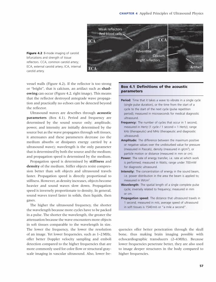
(CW) ultrasound that is not good for imaging because

no depth information can be derived. The percentage

of time that the sound source uses to emit pulses as

opposed to the listening part of the pulse repetition

period is described by the duty factor :

Duty factor pulse duration/

pulse repetition period

(%) (

)

=×1000

For the continuous wave ultrasound it is 100% (Figure

4.5 ). Note that two transducers are required with the

CW mode: one for constantly emitting sound and

another for constantly receiving echoes. No depth

discrimination is possible and CW is not used for

spatial pulse length, that is the distance that a pulse

occupies in space from the start to the end of the pulse.

Spatial pulse length mm number of cycles

wavelength mm

( )

( )

=×

Shorter pulses produce more accurate images because

resolution is improved by sampling smaller amounts

of tissue at a time.

To create an image or a waveform, ultrasound

machine needs to send a pulse and then stop and

listen to arriving echoes. This is the principle behind

pulsed wave (PW) ultrasound. If the machine emits

pulses all the time, it produces continuous wave

Figure 4.5 Continuous (CW) and pulsed wave

(PW) ultrasound modes.

Continuous wave

Pulsed wave

Two transducersemitting and receiving

One transduceremits then receives


60

imaging. PW requires only one transducer, which

fi rst emits and then detects returned echoes. Timing

of the returned echoes is then used for depth

discrimination.

Typically, with pulsed wave ultrasound imaging, the

duty factor is 0.2–0.5%, meaning that over 99% of the

time the ultrasound machine is listening as opposed

to emitting pulses. However, it emits short-duration

pulses thousands of times each second and that creates

an illusion of real-time imaging and a constant emis-

sion of pulses. In summary, by adjusting the imaging

depth or Doppler velocity scale, sonographers change

the pulse repetition period, PRF, and duty factor.

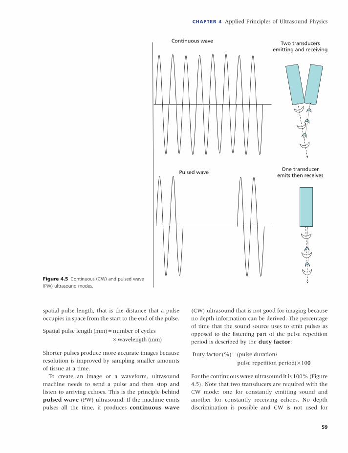
How does an ultrasound machine determine the

depth from which the returned echoes originated? As

shown in Figure 4.6 , a single-gate spectral Doppler

system is able to display the depth of insonation.

Several assumptions are built into sampling the

returned echoes from the depth set on the spectral

Doppler machine display (Figure 4.6 a). First, a pulse

is emitted and then the transducer becomes inactive

for the time necessary for the wave to reach 64 mm

depth and then for the return echoes to come back.

The theoretical time for this round trip would be:

distance (0.0064 m) divided by the average speed of

sound in soft tissues (1540 m/s) times two for the

round trip = 8.3 microseconds (Figure 4.6 b). There-

fore, a transcranial Doppler (TCD) unit opens the gate

right about that time to listen to returned echoes. The

gate is the time interval at which the transducer is

switched to the listening mode and arriving echoes are

detected, amplifi ed, and processed. When the gate

closes, the next pulse is emitted and the process is

repeated many times a second (Figure 4.6 c). If the

listening time interval is set too short, it creates a small

gate or sample volume. This can make sampling more

precise (and generate sharper images with ultrasound

imaging tests); however, it will limit the sensitivity of

TCD to detect fl ow because intracranial arteries are

small and any transducer movement may dislodge the

beam off the intercept.

Furthermore, an ultrasound beam has three dimen-

sions, ultrasound pulses have spatial length, and the

beam encounters structures that can change propaga-

tion speed by thousands of meters per second. This

creates some uncertainty and potential for error.

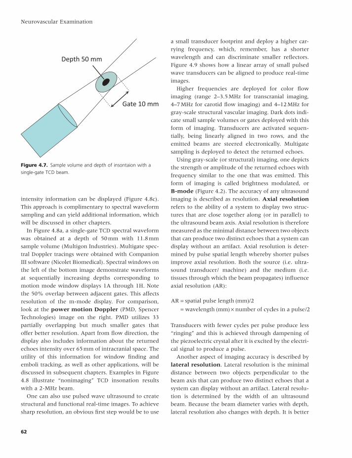
Figure 4.7 illustrates the principle of sample volume

or gate.

As a 2-MHz ultrasound wave leaves the transducer

and goes through the near fi eld , it then narrows to

the beam minimal diameter in the focal zone . The

distance from the transducer to this focus (or minimal

diameter) is also known as the focal length. After a

depth of 50 mm, a 2-MHz beam diverges into the far

fi eld. The beginning of beam widening marks the

beginning of the far zone or Fraunhofer zone .

If the depth of insonation is also set at 50 mm, 90%

of the returned Doppler signal will originate from

within the 3 mm core (the black oval area depicted in

Figure 4.7 ) and another 10% of the signal will come

from the three-dimensional sample of tissues around

it. Think of this sample volume (or gate ) as the

depth range that can be sampled. The sum of standard

deviations from the set depth of insonation is the

length of the sample volume along the ultrasound

beam axis, that is depth 50 mm ± 5 mm yields a gate

of 10 mm. This means that if a signal is detected at a

depth of 50 mm it can in theory originate anywhere

from within 45 mm to 55 mm depth. Obviously, the

core should yield the best returned signals but a bright

refl ector on the periphery of the sample volume can

also produce detectable echoes.

By analogy, think about an ultrasound beam like a

fl ashlight. If you walk at night and point the fl ashlight

at the ground, you only see the surface illuminated by

the beam footprint. You can control how much you

see by reducing the size of the light spot or making it

larger. Although this example is more pertinent to

beam focusing using a lens (which will be discussed

below), changing the gate or sample volume during

ultrasound exposure also changes the amount of

tissues being sampled.

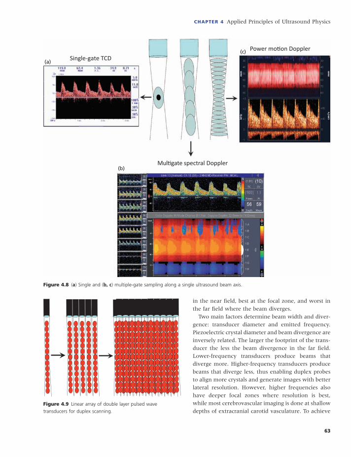
After echoes are detected by a single element TCD

transducer, several things happen during postprocess-

ing of the received echoes. Timing is everything. If the

instrument is set to listen to only one depth of insona-

tion, TCD provides a single-gate measurement (Figure

4.8 a). Once a pulse is emitted, a TCD instrument can

listen to several time epochs, and measurements will

be multigated . Often these spectral Doppler multi-

gate measurements overlap substantially (as shown

in the multigate example in Figure 4.8 b) where the

sonographer can control and change an overlap

between gates. Finally, numerous gates can be set for

sampling (power motion mode TCD machines usually

offer 33 to 250 gates), and fl ow direction as well as


61

Figure 4.6 Single-gate pulsed wave sampling of the depth set at 64 mm (see text for an explanation).

(a)

Time for a roundtrip

64 mm1540 m/s

X 2

(b)

Depth from emi ng surface 64 mm

(c)


62

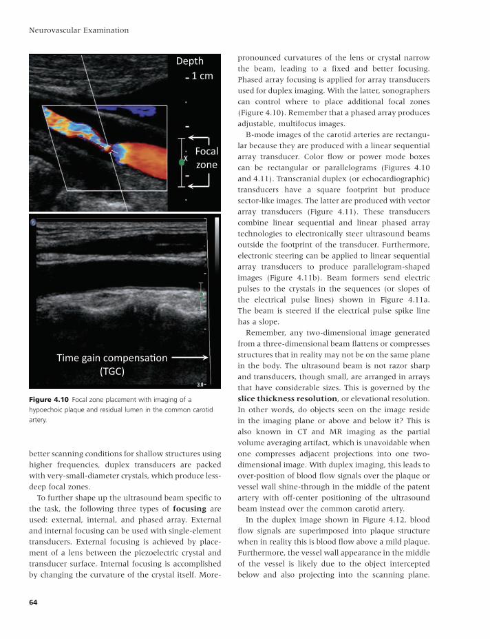
a small transducer footprint and deploy a higher car-

rying frequency, which, remember, has a shorter

wavelength and can discriminate smaller refl ectors.

Figure 4.9 shows how a linear array of small pulsed

wave transducers can be aligned to produce real-time

images.

Higher frequencies are deployed for color fl ow

imaging (range 2–3.5 MHz for transcranial imaging,

4–7 MHz for carotid fl ow imaging) and 4–12 MHz for

gray-scale structural vascular imaging. Dark dots indi-

cate small sample volumes or gates deployed with this

form of imaging. Transducers are activated sequen-

tially, being linearly aligned in two rows, and the

emitted beams are steered electronically. Multigate

sampling is deployed to detect the returned echoes.

Using gray-scale (or structural) imaging, one depicts

the strength or amplitude of the returned echoes with

frequency similar to the one that was emitted. This

form of imaging is called brightness modulated, or

B-mode (Figure 4.2 ). The accuracy of any ultrasound

imaging is described as resolution. Axial resolution

refers to the ability of a system to display two struc-

tures that are close together along (or in parallel) to

the ultrasound beam axis. Axial resolution is therefore

measured as the minimal distance between two objects

that can produce two distinct echoes that a system can

display without an artifact. Axial resolution is deter-

mined by pulse spatial length whereby shorter pulses

improve axial resolution. Both the source (i.e. ultra-

sound transducer/ machine) and the medium (i.e.

tissues through which the beam propagates) infl uence

axial resolution (AR):

AR spatial pulse length mm /

wavelength mm number of cyc

== ×

( )

( )

2

lles in a pulse/2

Transducers with fewer cycles per pulse produce less

“ringing” and this is achieved through dampening of

the piezoelectric crystal after it is excited by the electri-

cal signal to produce a pulse.

Another aspect of imaging accuracy is described by

lateral resolution . Lateral resolution is the minimal

distance between two objects perpendicular to the

beam axis that can produce two distinct echoes that a

system can display without an artifact. Lateral resolu-

tion is determined by the width of an ultrasound

beam. Because the beam diameter varies with depth,

lateral resolution also changes with depth. It is better

intensity information can be displayed (Figure 4.8 c).

This approach is complimentary to spectral waveform

sampling and can yield additional information, which

will be discussed in other chapters.

In Figure 4.8 a, a single-gate TCD spectral waveform

was obtained at a depth of 50 mm with 11.8 mm

sample volume (Multigon Industries). Multigate spec-

tral Doppler tracings were obtained with Companion

III software (Nicolet Biomedical). Spectral windows on

the left of the bottom image demonstrate waveforms

at sequentially increasing depths corresponding to

motion mode window displays 1A through 1H. Note

the 50% overlap between adjacent gates. This affects

resolution of the m-mode display. For comparison,

look at the power motion Doppler (PMD, Spencer

Technologies) image on the right. PMD utilizes 33

partially overlapping but much smaller gates that

offer better resolution. Apart from fl ow direction, the

display also includes information about the returned

echoes intensity over 65 mm of intracranial space. The

utility of this information for window fi nding and

emboli tracking, as well as other applications, will be

discussed in subsequent chapters. Examples in Figure

4.8 illustrate “nonimaging” TCD insonation results

with a 2-MHz beam.

One can also use pulsed wave ultrasound to create

structural and functional real-time images. To achieve

sharp resolution, an obvious fi rst step would be to use

Figure 4.7. Sample volume and depth of insontaion with a

single-gate TCD beam.

Depth 50 mm

Gate 10 mm


63

in the near fi eld, best at the focal zone, and worst in

the far fi eld where the beam diverges.

Two main factors determine beam width and diver-

gence: transducer diameter and emitted frequency.

Piezoelectric crystal diameter and beam divergence are

inversely related. The larger the footprint of the trans-

ducer the less the beam divergence in the far fi eld.

Lower-frequency transducers produce beams that

diverge more. Higher-frequency transducers produce

beams that diverge less, thus enabling duplex probes

to align more crystals and generate images with better

lateral resolution. However, higher frequencies also

have deeper focal zones where resolution is best,

while most cerebrovascular imaging is done at shallow

depths of extracranial carotid vasculature. To achieve

Figure 4.8 ( a ) Single and ( b, c ) multiple-gate sampling along a single ultrasound beam axis.

Single-gate TCD

Mul gate spectral Doppler

Power mo on Doppler

(a)

(b)

(c)

Figure 4.9 Linear array of double layer pulsed wave

transducers for duplex scanning.


64

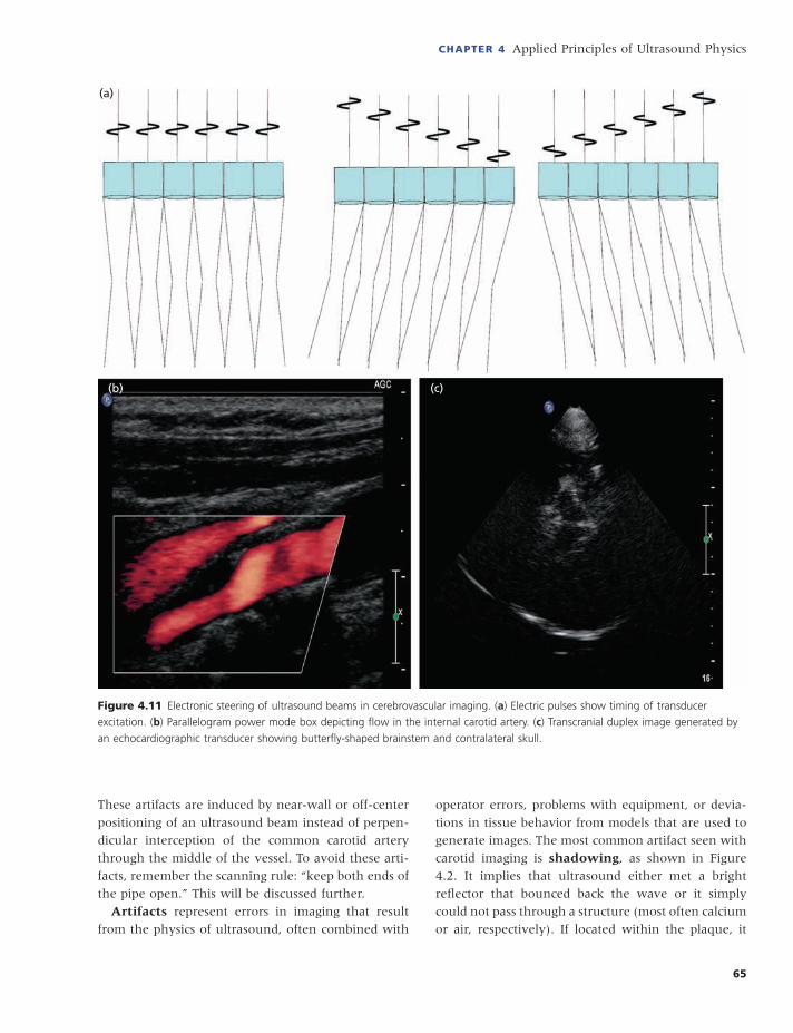
pronounced curvatures of the lens or crystal narrow

the beam, leading to a fi xed and better focusing.

Phased array focusing is applied for array transducers

used for duplex imaging. With the latter, sonographers

can control where to place additional focal zones

(Figure 4.10 ). Remember that a phased array produces

adjustable, multifocus images.

B-mode images of the carotid arteries are rectangu-

lar because they are produced with a linear sequential

array transducer. Color fl ow or power mode boxes

can be rectangular or parallelograms (Figures 4.10

and 4.11 ). Transcranial duplex (or echocardiographic)

transducers have a square footprint but produce

sector-like images. The latter are produced with vector

array transducers (Figure 4.11 ). These transducers

combine linear sequential and linear phased array

technologies to electronically steer ultrasound beams

outside the footprint of the transducer. Furthermore,

electronic steering can be applied to linear sequential

array transducers to produce parallelogram-shaped

images (Figure 4.11 b). Beam formers send electric

pulses to the crystals in the sequences (or slopes of

the electrical pulse lines) shown in Figure 4.11 a.

The beam is steered if the electrical pulse spike line

has a slope.

Remember, any two-dimensional image generated

from a three-dimensional beam fl attens or compresses

structures that in reality may not be on the same plane

in the body. The ultrasound beam is not razor sharp

and transducers, though small, are arranged in arrays

that have considerable sizes. This is governed by the

slice thickness resolution , or elevational resolution.

In other words, do objects seen on the image reside

in the imaging plane or above and below it? This is

also known in CT and MR imaging as the partial

volume averaging artifact, which is unavoidable when

one compresses adjacent projections into one two-

dimensional image. With duplex imaging, this leads to

over-position of blood fl ow signals over the plaque or

vessel wall shine-through in the middle of the patent

artery with off-center positioning of the ultrasound

beam instead over the common carotid artery.

In the duplex image shown in Figure 4.12 , blood

fl ow signals are superimposed into plaque structure

when in reality this is blood fl ow above a mild plaque.

Furthermore, the vessel wall appearance in the middle

of the vessel is likely due to the object intercepted

below and also projecting into the scanning plane.

better scanning conditions for shallow structures using

higher frequencies, duplex transducers are packed

with very-small-diameter crystals, which produce less-

deep focal zones.

To further shape up the ultrasound beam specifi c to

the task, the following three types of focusing are

used: external, internal, and phased array. External

and internal focusing can be used with single-element

transducers. External focusing is achieved by place-

ment of a lens between the piezoelectric crystal and

transducer surface. Internal focusing is accomplished

by changing the curvature of the crystal itself. More-

Figure 4.10 Focal zone placement with imaging of a

hypoechoic plaque and residual lumen in the common carotid

artery.

Depth 1 cm

Focal zone

Time gain compensa on (TGC)


65

operator errors, problems with equipment, or devia-

tions in tissue behavior from models that are used to

generate images. The most common artifact seen with

carotid imaging is shadowing , as shown in Figure

4.2 . It implies that ultrasound either met a bright

refl ector that bounced back the wave or it simply

could not pass through a structure (most often calcium

or air, respectively). If located within the plaque, it

These artifacts are induced by near-wall or off-center

positioning of an ultrasound beam instead of perpen-

dicular interception of the common carotid artery

through the middle of the vessel. To avoid these arti-

facts, remember the scanning rule: “keep both ends of

the pipe open.” This will be discussed further.

Artifacts represent errors in imaging that result

from the physics of ultrasound, often combined with

Figure 4.11 Electronic steering of ultrasound beams in cerebrovascular imaging. ( a ) Electric pulses show timing of transducer

excitation. ( b ) Parallelogram power mode box depicting fl ow in the internal carotid artery. ( c ) Transcranial duplex image generated by

an echocardiographic transducer showing butterfl y-shaped brainstem and contralateral skull.

(a)

(b) (c)


66

4.14 ), and propagation speeds of the two media must

be different. As a result, change in the transmission

speed will cause ultrasound to travel in a different

direction.

With oblique interception of a boundary between

two tissues (medium 1 and 2), further direction of the

beam is dependent on propagation speed difference.

If speed 1 is greater than 2, the transmission angle

(arrow in the green medium) is less than the incidence

angle (arrow in the blue medium). If speed 1 is less

than 2, the transmission angle is greater than the

incidence angle. The latter is particularly true with

TCD insonation through the temporal bone. If an

ultrasound beam encounters an object that is compa-

rable in its dimensions to the beam or wavelength,

scattering of attenuated echoes may occur in every

direction. This phenomenon is known as Rayleigh

scattering, and is proportionate to the forth power of

the emitted frequency. This scattering is organized and

red blood cells redirect ultrasound energy in every

indicates the presence of calcium. Shadowing is also

used to fi nd transverse processes and locate the verte-

bral artery on the neck (Figure 4.13 a). This artifact

(Figure 4.13 b) is also known as edge shadow or

shadow by refraction . Besides refraction, beam

redirection can also be caused by Rayleigh scatter-ing . Both phenomena are shown below (Figure 4.14 ).

Adventitia, intima, and adjacent red blood cells (small

refl ectors in the transverse projection, Figure 4.13 ) are

responsible for expanding shadows distal to the point

of ultrasound beam diversion and partial destruction.

Note that these shadows originate from the outer parts

of the common carotid artery transverse view where

the intercepted adventitia has the smallest diameter

comparable to ultrasound beam dimensions.

Refraction , or the change in the direction of ultra-

sound wave propagation, occurs when an ultrasound

beam travels from one medium to another at certain

conditions. First, the incidence angle of the beam

intercepting the boundary must be oblique (Figure

Figure 4.12 Slice thickness resolution and artifacts from refl ectors above and below the scanning plane.

Scanning plane

Object above

Object below

Plaque Superimposed flow

Par al volume averaging


67

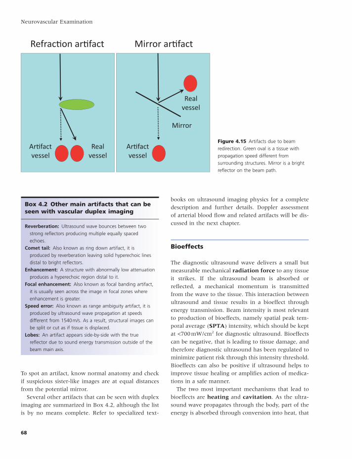
rection off a strong refl ector produces an artifact

known as mirror image . Remember that the artifact

is placed deeper than the real structure (Figure 4.15 ).

The real structure may not cause an artifact because

another refl ector, termed the mirror, is likely respon-

sible for it. For example, refl ections from pleura can

produce an image of two sublavian arteries. Adventitia

of the CCA can produce artifi cial color fl ow projection.

direction. Although these phenomena are totally dif-

ferent, they produce changes in sound propagation

and beam direction.

Refraction redirects the ultrasound beam and

degrades lateral resolution. It can also produce a

refraction artifact where a false image of a structure

resides side by side (or at the same depth) as the real

image (Figure 4.15 ). Ultrasound refl ection and redi-

Figure 4.13 Examples of shadowing

artifact with carotid and vertebral duplex

scanning. ( a ) A transverse process (TP)

casts a shadow over the vertebral artery

(VA), and this shadow is used to locate

intratransverse views of the VA.

( b ) Shadow produced by a noncalcifi ed

carotid vessel wall intercepted

cross-sectionally.

(a) (b)

Figure 4.14 Beam redirection with

refraction and Rayleigh scattering.

Refrac on Speed 1 = speed 2

Speed 1 > speed 2

Speed 1 < speed 2

Medium 1 Medium 2

Rayleigh sca ering

Wavelength and emi ed pulse

amplitude

Reflected echo amplitude and

direc on

Red blood cell


68

books on ultrasound imaging physics for a complete

description and further details. Doppler assessment

of arterial blood fl ow and related artifacts will be dis-

cussed in the next chapter.

Bioeffects

The diagnostic ultrasound wave delivers a small but

measurable mechanical radiation force to any tissue

it strikes. If the ultrasound beam is absorbed or

refl ected, a mechanical momentum is transmitted

from the wave to the tissue. This interaction between

ultrasound and tissue results in a bioeffect through

energy transmission. Beam intensity is most relevant

to production of bioeffects, namely spatial peak tem-

poral average ( SPTA ) intensity, which should be kept

at < 700 mW/cm 2 for diagnostic ultrasound. Bioeffects

can be negative, that is leading to tissue damage, and

therefore diagnostic ultrasound has been regulated to

minimize patient risk through this intensity threshold.

Bioeffects can also be positive if ultrasound helps to

improve tissue healing or amplifi es action of medica-

tions in a safe manner.

The two most important mechanisms that lead to

bioeffects are heating and cavitation . As the ultra-

sound wave propagates through the body, part of the

energy is absorbed through conversion into heat, that

To spot an artifact, know normal anatomy and check

if suspicious sister-like images are at equal distances

from the potential mirror.

Several other artifacts that can be seen with duplex

imaging are summarized in Box 4.2 , although the list

is by no means complete. Refer to specialized text-

Figure 4.15 Artifacts due to beam

redirection. Green oval is a tissue with

propagation speed different from

surrounding structures. Mirror is a bright

refl ector on the beam path.

Ar fact vessel

Realvessel

Realvessel

Ar fact vessel

Mirror

Refrac on ar fact Mirror ar fact

Box 4.2 Other m ain a rtifacts that c an b e s een with v ascular d uplex i maging

Reverberation: Ultrasound wave bounces between two

strong refl ectors producing multiple equally spaced

echoes.

Comet tail: Also known as ring down artifact, it is

produced by reverberation leaving solid hyperechoic lines

distal to bright refl ectors.

Enhancement: A structure with abnormally low attenuation

produces a hyperechoic region distal to it.

Focal enhancement: Also known as focal banding artifact,

it is usually seen across the image in focal zones where

enhancement is greater.

Speed error: Also known as range ambiguity artifact, it is

produced by ultrasound wave propagation at speeds

different from 1540 m/s. As a result, structural images can

be split or cut as if tissue is displaced.

Lobes: An artifact appears side-by-side with the true

refl ector due to sound energy transmission outside of the

beam main axis.


69

safety precaution for diagnostic ultrasound: minimize

the time of overall patient exposure to ultrasound.

Furthermore, special clinical situations require con-

tinuous TCD monitoring that is safe in patients under-

going emboli detection or even receiving thrombolysis

with intravenous tissue plasminogen activator. There

is a possibility that even low-power diagnostic ultra-

sound could produce other bioeffects, such as revers-

ible disaggregation of fi brin strands in the thrombus,

increase in streaming of plasma around and through

the thrombus, delivery of medications to tissues with

compromised perfusion, and release of nitric oxide

inducing vasodilation. Examples of harvesting both

harmful and positive bioeffects include the develop-

ment of high-intensity focused ultrasound (HIFU)

therapeutic systems for tissue ablation through ther-

mal and cavitational mechanisms, and sonothrom-

bolysis for acute stroke likely through an increased

tissue plasminogen activator (tPA) delivery to the

thrombus, promotion of its fi brinolytic activity, and

possibly vasodilation.

This brief introduction by no means covers the vast

fi eld of ultrasound physics nor all the terminology,

defi nitions, and explanations that clinicians should

know in order to perform and interpret ultrasound

tests. More information can be found in specifi c text-

books dealing with ultrasound physics and instrumen-

tation in the Recommended Reading list.

Recommended reading

Edelman SK . Understanding Ultrasound Physics , 4th edn. ESP

Inc , 2012 .

Kremkau F. Sonography Principles and Instruments , 8th edn.

St Louie , Missouri : Saunders , 2010 .

Valdueza JM , Shreiber SJ , Roehl JE , Klingebiel R . Neu-

rosonology and Neuroimaging of Stroke . Stuttgart, Germany :

Thieme , 2008 .

Current study materials offered by Davies Publishing:

http://www.daviespublishing.com .

is the thermal mechanism. The thermal index pre-

dicts the maximum temperature raise under given

insonation conditions. It is reported for the following

tissues: TIS, for soft tissues; TIB, for bones; and TIC,

for cranial bone. The latter could be shown on a TCD

display. Diagnostic ultrasound can cause temperature

elevations, usually not exceeding 2 degrees Celsius

and prolonged (up to 50 hours) exposure to diagnostic

ultrasound showed no damage to insonated tissues.

Cavitation describes creation of gaseous nuclei

from dissolved gases in a fl uid exposed to ultrasound,

that is the nonthermal mechanism. Cavitation can be

induced as stable or transient. Stable cavitation occurs

at lower peak negative pressures when formed gaseous

nuclei tend to oscillate in size but do not burst. Tran-

sient cavitation is produced by higher peak negative

pressures and leads to bursting of gaseous nuclei. It is

also known as inertial cavitation. The likelihood of

harmful bioeffects due to cavitation is predicted by

the mechanical index (MI). MI is related to peak

negative pressure and emitted ultrasound frequency.

Higher MI values are associated with greater peak

negative pressures and lower frequencies. An easier

way to remember what MI and TI refl ect is the expres-

sion: “shake and bake” referring to cavitation and

thermal effects respectively.

The American Institute of Ultrasound in Medicine

(AIUM) has stated that no harmful bioeffects have

been reported to date from exposure to diagnostic

ultrasound. To minimize patient exposure to ultra-

sound energy, sonographers should follow the ALARA

principle: as low as reasonably achievable. With TCD

examination, this is done by reducing power of the

emitted signal to 10% when investigating through

the orbit, burr hole, craniotomy site, or fontanelle.

A transtemporal examination through intact skull

should start with 100% power, seemingly violating

the ALARA principle. However, this allows a window

to be found faster or to be found in a patient who has

suboptimal windows, and thus the examination can

be completed faster. Therefore, it satisfi es the second

Documents

Neurovascular Examination (The Rapid Evaluation of Stroke Patients Using Ultrasound Waveform Interpretation) || Applied Principles of Ultrasound Physics