NeuroMaps Mapper

The Mapper is a stand-alone application for mapping data

to brain atlases for presentation and publication.

Image data are mapped to a stereotaxic MRI atlas of

the macaque brain or the mouse brain.

This tutorial shows how mapping to a standard atlas

adds value to image data.

It illustrates mapping an area to the macaque

atlas but is equally applicable to the mouse atlas.

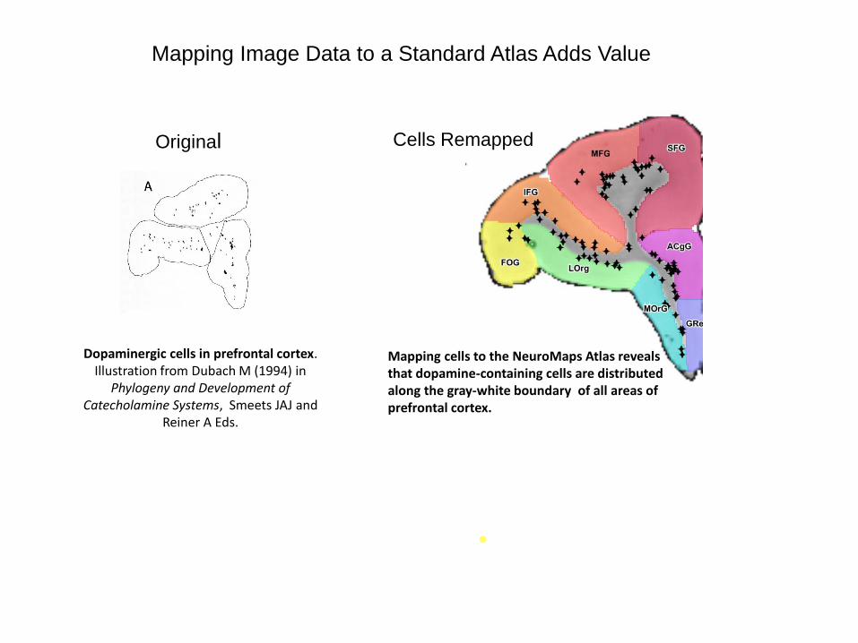
Dopaminergic cells in prefrontal cortex. Illustration from Dubach M (1994) in

Phylogeny and Development of Catecholamine Systems, Smeets JAJ and

Reiner A Eds.

Mapping cells to the NeuroMaps Atlas reveals that dopamine-containing cells are distributed along the gray-white boundary of all areas of prefrontal cortex.

Original Cells Remapped

Mapping Image Data to a Standard Atlas Adds Value

Lateral prefrontal cortex lesioncausing top-down attentional deficit .

Rossi, A. F. et al., Journal of Neuroscience 27:11306-11314 (2007) Mapping the lesion to a lateral surface view

of the NeuroMaps Atlas shows that the lesion involves the superior, middle, inferior, and fronto-orbital gyri of the frontal lobe

Original

Lesion Remapped

Mapping Image Data to a Standard Atlas Adds Value

Sites of positive and negativereinforcement

by electrical brain stimulation Bowden DM (unpublished)

Hi PositiveMed Positive Lo Positive

NegativeNo Effect

Color coding of positive and negative sites makes salient

the grouping of sites by reinforcement value.

Mapping Image Data to a Standard Atlas Adds Value

Expression of gene GUCY1A3 in infant macaques subjected to maternal deprivationSabatini, M. J. et al., Journal of Neuroscience 2007;27:3295-3304

Hi expressionMed expressionLo expression

Color coding level of expression makes salient its distribution in different structures and within layers of cerebral cortex.

Mapping Image Data to a Standard Atlas Adds Value

This tutorial

will illustrate

mapping cortical

area 4(F1)

from a page in the

rhesus macaque atlas

of

Paxinos, Huang & Toga

(2000)

to the

NeuroMaps Macaque

Brain Atlas

To download the Mapper the first time, go to BrainInfo: http://braininfo.org

Click ‘Map/Edit/Print Your Data in Atlas’

After the first download you will enter the Mapper directly from your desktop

You will follow the instructions in BrainInfo for download

and installation of the Mapper

When you have opened the folder below, double click ‘mapper-macaque.jar’

On the opening page:

Click: ‘Map New Image’

Navigate in your directory to the figure provided in the

Mapper ‘sample_data’ folder that you installed.

Open: Paxinos Figure72.jpg

navigate

Click: ‘New Study’

Enter a name for the study, e.g., ‘Mapper Tutorial’

Click: ‘OK’

Click: ‘Open the Atlas’

Note the ‘i’ icon next to each tool. If you are ever confused, do not

hesitate to click it.

The Atlas appears as a 2D coronal plane through the center of the

anterior commissure (AP 0). The next couple of slides are a detour

to show how to obtain different views for mapping. To see

the choice of surface views, click the ‘Surface’ button.

From here on, click Continue or Next Step (bottom right) to proceed.

For other views, click the button labeled ‘Atlas’ here (upper right corner

of the sidebar) and step through the six views circled below.

Run your cursor over a structure and see its name at the top of the panel.

Click the structure to see BrainInfo’s page about it…Continue

This is the MRI surface view.

To return to the coronal cross-sectional view,

You will click the button to select ‘Section’.

Continue

Click the ‘In’, ‘Out’, and ‘Move’ buttons (circled top) and then click on the

Atlas to adjust its size and location. We want to map to the opposite side

of the Atlas, so click ‘Horizontal’. Match the Atlas plane of section to the data

image using the Slider for AP adjustment and the pie icon to tilt and rotate the

plane of section. (AP -8.10 & bottom tilt 1.5o in this case.) Next Step

Having adjusted the plane of section of the Atlas to match the data image,

Click ‘Align Image with Atlas’ to proceed.

Here you can, if necessary, rotate the image to match the atlas by

clicking the ends of the double-headed arrow. (Not necessary in

this case)

And here you can adjust the size of either or both images roughly to match.

Click the circled button. Here, click and drag in the left panel to create a box

around the part of the Atlas image to which you want to map.

Do the same to create a box around the equivalent area of the data image.

When you click ‘Continue’, the images will snap to the same size.

Click ‘Map Image to Atlas’

Click ‘Select Equivalent Points’. Then click pairs of equivalent landmark points in

the two images. It is good to click the first four pairs near the top, bottom, left and

right sides of the image.

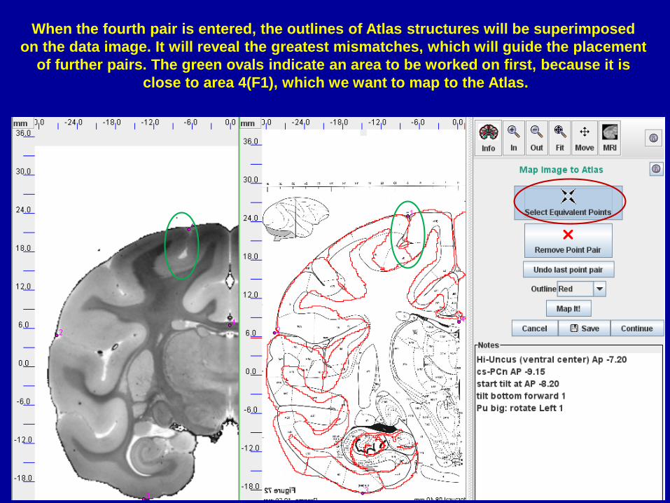
When the fourth pair is entered, the outlines of Atlas structures will be superimposed

on the data image. It will reveal the greatest mismatches, which will guide the placement

of further pairs. The green ovals indicate an area to be worked on first, because it is

close to area 4(F1), which we want to map to the Atlas.

Having mapped pairs of landmarks to bring the borders of the sulcus into line, we

see that the medial boundary of the gyrus has been pulled left of the Atlas boundary.

The next step will be to bring that into line.

Clicking a few more pairs brings the midline and gray-white boundaries of the

gyrus into line.

If you will want to map other areas in addition to area 4(F1), you can click a

number or other point-pairs on the inner and outer boundaries of the cortex to

bring the rest of the Atlas template into an adequate fit to map (warp) the data image

to the Atlas. Click ‘Map It!’ and Continue.

You can judge the extent of the warp by the distortion of the scales on the data image.

The next step is to define the boundaries of area 4(F1) and create an Atlas overlay for it.

Click ‘Make or Edit Atlas Overlays’

The template boundaries have been superimposed on the data image.

You will now trace the boundary of area 4(F1) to create an overlay by that name.

Click ‘New Overlay’

Enter the name of the area in the ‘Choose a name’ box.

Click ‘OK’

To select the color you want for the overlay:

Click ‘Color

We have elected to keep the default color ‘turquoise’

Click ‘Close’

Insert slide in mid drawing of 4(F1) boundaries.

We have zoomed area 4(F1) for greater cursor control and changed the Outline

Color to ‘Green’ for contrast with the tracing color (magenta). We have set Data Type

to ‘Area Data’ and clicked ‘Draw to Template’, so that, as our cursor traces the

boundary in the data image, the Mapper snaps it to the nearest Atlas boundary…

the two will exactly coincide. We have clicked a starting point and dragged right.

When we reached the point where the boundary crossed to the inner surface of

the cortex (arrow). We switched to the ‘Free Draw’ tool and clicked the inner surface

of the cortex. The Mapper ceased to follow the Atlas outline and created a straight

line across the cortex. Alternating between the two tools, we continued to trace the

boundary and completed the overlay by clicking the starting point.

Here we have clicked the ‘Add Label’ button and clicked the place we wanted it

to appear on the overlay.

By displaying and comparing each data area mapped to the Atlas against that

of the original data image, one can alternate between mapping and checking until

all data areas have been overlaid on the Atlas. (See next slide.)

This illustrates all areas from the zero plane of the Paxinos et al. rhesus atlas

Mapped to the NeuroMaps Macaque Atlas.

Once you have mapped all of the data areas

as overlays to the Atlas, you can submit it

to the NeuroMaps Editor to prepare

for presentation or publication.

Click: ‘Edit and Export for Printing’

Enter the name of the Investigator (the person

responsible for the study) and Your Name

(the person editing the image). They may,

as here, be the same. Then:

Click: ‘Edit and Export for Printing

This is a section from prefrontal

cortex with overlays for all

cytoarchitectonic areas.

To create a figure for publication,

set the resolution in dots per inch

(dpi usually = 300) and the size

(width in millimeters) to match

publisher’s specifications.

To enlarge the image to 300 mm,

for example,

Click: ‘width (mm)’

Here the architectonic areas are

overlaid on the atlas MRI. You may

prefer to present them against a

plain white background.

Click the arrowhead of the

message box that shows MRI and

select ‘Lines’ .

This shows the overlays against a

white background.

To add or remove a label:

Click: Add/Remove Label or Symbol

and click the site where you want it.

To change the size of labels:

Click: up and down arrows

next to ‘label/symbol size’

To change the colors of overlays:

Click: Edit/Color Overlays

This chart allows you to

• Show or not show each overlay

• Make an overlay opaque (partially

translucent) so the MRI shows thru

• Select a different color for an

overlay from a color chart

• Change a label from black (default)

to white

• Show a label against a contrasting

background of black or white.

When you finish editing

Click: ‘Save and Export’ (upper right)

Navigate to the folder on your

computer where you want to save

the figure

Assign a name to the figure

Click: ‘Save’

Happy Mapping!BrainInfo/NeuroMaps

http://braininfo.org

Douglas M. Bowden, MD

National Primate Research Center

University of Washington, Seattle