)M-37

NASA Technical Memorandum 107108

Neural Network Models of Simple Mech'anical Systems Illustrating the Feasibility of Accelerated Life Testing

Steven P. Jones and Ralph Jansen Ohio Aerospace Institute Cleveland, Ohio

Robert L. Fusaro Lewis Research Center Cleveland, Ohio

Prepared for the Annual Meeting sponsored by the Society of Tribologists and Lubrication Engineers Cincinnati, Ohio May 19-23, 1996

National Aeronautics and Space Administration

)

https://ntrs.nasa.gov/search.jsp?R=19960031943 2018-08-24T16:37:07+00:00Z

NEURAL NETWORK MODELS OF SIMPLE MECHANICAL SYSTEMS ILLUSTRATING THE FEASIBILITY OF ACCELERATED LIFE TESTING

Steven P. Jones· and Ralph Jansen Ohio Aerospace Institute

Cleveland, Ohio

Robert L. Fusaro National Aeronautics and Space Administration

Lewis Research Center Cleveland, Ohio

SUMMARY

A complete evaluation of the tribological characteristics of a given material/mechanical system is a time-consuming operation since the friction and wear process is extremely systems sensitive. As a result, experimental designs (i.e., Latin Square, Taguchi) have been implemented in an attempt to not only reduce the total number of experimental combinations needed to fully characterize a materiaUmechanical system, but also to acquire life data for a system without having to perform an actual life test. Unfortunately, these experi­mental designs still require a great deal of experimental testing and the output does not always produce meaningful information. In order to further reduce the amount of experimental testing required, this study employs a computer neural network model to investigate different material/mechanical systems. The work focuses on the modeling of the wear behavior, while showing the feasibility of using neural networks to predict life data. The model is capable of defining which input variables will influence the tribological behavior of the particular material/mechanical system being studied based on the specifications of the overall system.

INTRODUCTION

Recent advances in computer and electronics technology have greatly increased the reliability and longevity of electronic systems, which have long been considered to be the limiting life factor for satellites. As a result of these improvements, mechanical systems have now become a major life-limiting factor in current satellite systems (refs. 1 to 7). Recently, a number of significant spacecraft anomalies have occurred from problems with mechanically moving mechanisms such as bearings, gimbals, latches, and hinges (refs. 4 to 8). It has become evident that as mission durations extend beyond 5 years, further advances in the reliability and longevity of mechanical space systems will be required.

Verification testing is an important aspect of the design process for mechanical mechanisms. Full scale, full length life testing is typically used to space qualify any new component. However, as the required life specification is increased, full length life tests become more costly and also lengthen the development time. In addition, this type of testing becomes prohibitive as the mission life exceeds 5 years, primarily because of the high cost and the slow turnaround time for new technology. As a result, accelerated testing techniques are needed to reduce the time required for testing mechanical components.

Current accelerated testing methods typically consist of increasing speeds, loads, or temperatures in order to simulate a high cycle life in a short period of time. However, two significant drawbacks exist with this technique. The first is that it is often not clear what the accelerated factor is when the operating conditions are modified. Second, if the conditions are changed by a large degree, on a scale of an order of magnitude or more, the mechanism is forced to operate out of its design regime. Operation in this condition can often exceed material/mechanical systems parameters and renders the test meaningless.

It is theorized that neural network systems may be able to model the operation of a mechanical mechanism. If so, these neural network models could then be used to simulate long term mechanical testing using data from a short term test. This combination of computer modeling and short term mechanical testing could then be used to verify the reliability of mechanical systems, thereby eliminating the costs associated with long term testing. Neural network models could also enable designers to predict performance of

*Current Affiliation: NRC Fellow, Phillips Laboratory, Propulsion Directorate, Carbon Materials Research Group, Edwards AFB,CA.

mechanisms at the conceptual design stage by entering the critical parameters as inputs and running the model to predict performance.

The purpose of this study was to assess the potential of using neural networks for predicting the per­formance and life of a mechanical system. To accomplish this, a neural network system was generated to model previously taken data from (1) pin-on-disk, (2) line contact rub shoe, and (3) four-ball tribometers. Critical parameters such as load, speed, oil viscosity, temperature, sliding distance, friction coefficient, wear, and material properties were used to produce models for each tribometer. A methodology was then developed in order to use each model to predict the results of tests under conditions which were different that those used to predict the model.

BACKGROUND ON NEURAL NETWORKS

Neural Network Overview

Artificial neural networks are not new to the scientific community. They have been utilized in many applications since the late 1940's, when D.O. Hebb proposed a learning law that became the starting point of artificial neural network training algorithms (ref. 9). Only recently, though, has the power of the neural network model been realized and research into new application areas been started. Generally speaking, the artificial neural network is a powerful computing algorithm that mimics the functionality (i.e., neuron cells) of the human brain. They learn by trial and error directly from data in a manner analogous to the way a biological brain learns from sensory input. Thus, neural networks can be taught to analyze and model complex, nonlinear processes that are not well understood. Once these networks have "learned" the processes involved in the application, they are able to identify, extract. and characterize hidden patterns within the data that are difficult to observe by other analytical techniques. From this initial data, the network can then predict the output of a trial based on a limited amount of input.

It should also be noted that one of the advantages to a neural network model is its insensitivity to minor variations in its input. Essentially. the network is able to ignore noise and slight scatter in the data and focus on the underlying relationships between variables. However. it should be noted that neural networks are only as good as the input/output data used to train the model.

Basic Structure and Operation

Although many types of neural networks exist. they all have three things in common. The network can be described in terms of its individual neurons, the connections between them (topology), and its learning rule (ref. 10). The following section discusses the fundamental structure and operation of neural networks.

The Artificial Neuron

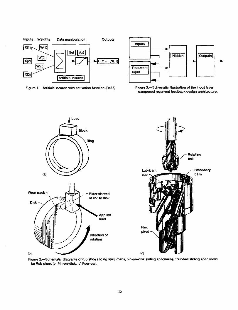
As the concept of neural networks was evolving. the artificial neuron was designed to mimic the first order characteristics of the biological neuron. Each input to a neuron represents the output of a neuron from a previous layer. The initial input values must be scaled from their numeric range into a range that the neural network deals with efficiently. Two ranges are commonly used in network design-[O,I] and [-1,1]. Generally, linear, logistic. and hyperbolic tangent functions are used to scale the input data. The input is then multiplied by a weight factor (analogous to a synaptic strength in biology). and the weights are then summed to deter­mine an activation level of the neuron. The activation levels are then further manipulated by an activation. or transfer. function to obtain the neuron's output signal. In many instances. this transfer function is the logistic. or sigmoid. function. which has the form f(x) = 1/(1 +e-X ), although the transfer function can be any function simulating the nonlinear characteristics of the system. A schematic of this process is shown in figure 1. By utilizing multiple layers of neurons. with multiple neurons in each layer, more complex relationships can be modeled.

With this type of architecture. though, the output is solely dependent on the current input variables and the values of their weights. However. recurrent architectures, which are also investigated in this study. recirculate previous outputs back to neurons in the same or previous layer. Hence. their output is generated from current inputs/weights. as well as from previous outputs. For this reason. recurrent networks are said to have characteristics very similar to short-term memory in humans.

2

Even with the organization of neurons into various architectures, the network cannot function unless it has the ability to learn from the given inputs and outputs. This concept is the premise behind the training algorithms used in neural network development. Training is accomplished by sequentially applying inputs and adjusting the corresponding weights according to a specified procedure until the desired output value is obtained. During the course of training, the network weights for each input will converge to a specific value, such that values approximately equal to the desired output are obtained. Network training is completed when further modifications of the input weights do not produce closer approximations of the output values (i.e., the error between actual and approximate output values is minimized). The weights for each input can then be analyzed to determine the impact that variable has on producing the correct output. Larger weights on specific input variables mean that those variables have a stronger influence on the output parameter. This is referred to as determining the contribution strength of the input variable.

The training algorithm used in the designs studied in this work is known as backpropagation. Back­propagation, which had its beginning in 1974 with the work of Werbos (ref. II), is a systematic method for training multilayer networks. The development of this training algorithm is directly responsible for the advancement of the field of artificial neural networks over the last 20 years. However, the topic of back­propagation is too complex for this paper, so the reader is referred elsewhere (ref. 12).

EXPERIMENTAL PROCEDURE

Data Sets Used

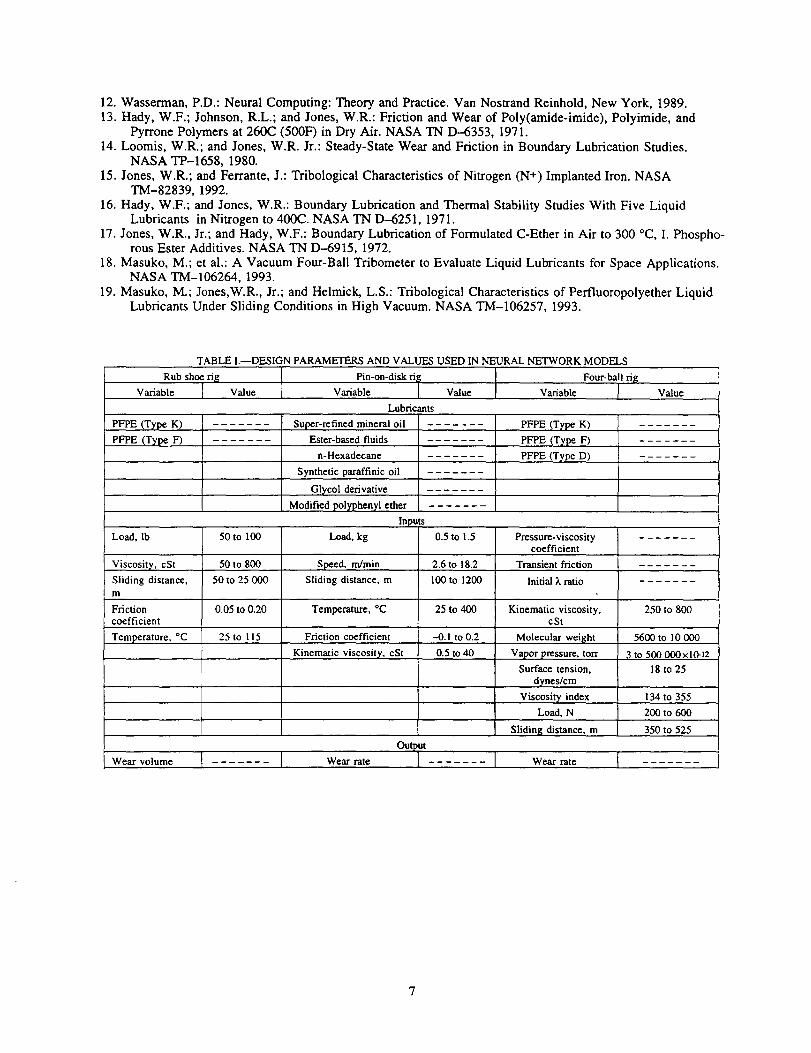
The data sets used in the three models developed in this work were obtained from various researchers, projects, and test rigs at the NASA Lewis Research Center. Each model was developed according to the material systems and test variables associated with the individual test rigs. The following sections will define the data sets and test variables used for each model developed in this work. The data for each model is given in Appendixes A to F.

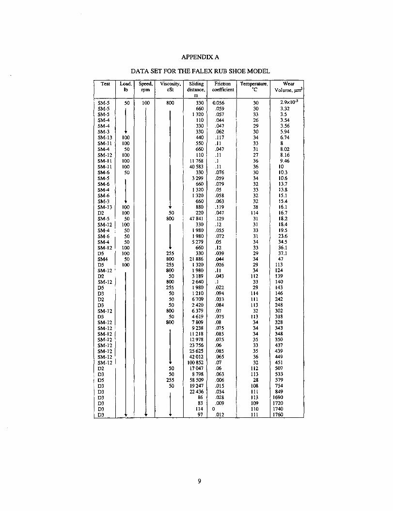
The first network developed modeled data from a line contact rub shoe rig. A schematic diagram of this rig is shown in figure 2(a). The data set used for the training and testing of this model was accumulated from unpublished NASA data. All of the tests used in this data set were run using 440C stainless steel speci­mens at a constant speed of 100 rpm (0.1833 mls). Table I lists the parameters that were varied in these tests as well as their ranges. The output variable for this model was the cumulative wear volume. This was used instead of a calculated wear rate parameter, since the calculation of accurate wear rates from the available data would have significantly reduced the number of data points available to train the model. By using this output variable, however, the amount of scatter in the model is increased, because wear volume is not constant from sample to sample.

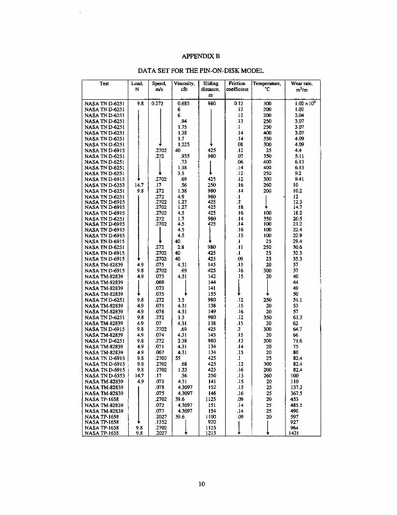
The second model generated in this work utilized data from several early NASA Technical Memorandums (refs. 13 to 17), which investigated the tribological properties of various materials using a pin­on-disk apparatus, shown schematically in figure 2(b). Table I defines the parameters, materials, and ranges used in this model. Various materials, including polymers and steel, were used for the pins. while M50 steel was used as the disk material.

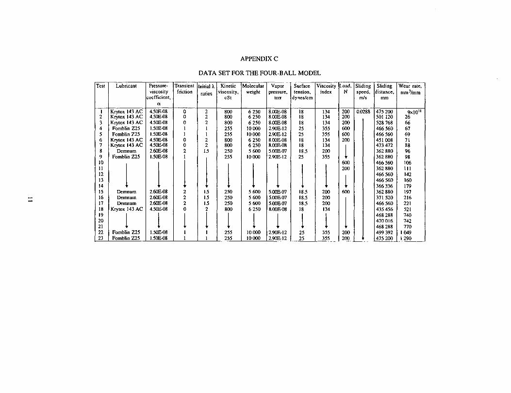
The final model generated in this work used published and unpublished NASA data which utilized a four-ball test rig, shown schematically in figure 2(c) (ref. 18). The specimen material for the balls was 440C stainless steel, and three perfluoropolyether (PFPE) fluids (Type K, Type F, and Type D) were used as lubri­cants. All specimens were run at a uniform speed of 0.0288 mls. Since there was little variation in the ranges of the test variables, the focus of the model was on determining the tribological properties of various lubricants from extensive materials properties and limited test properties. Table I lists the properties and variables used for this model. Several of the material properties, the transient friction and initial I.. ratio, were utilized in this work to provide general information on the lubricants behavior under the test rig conditions (i.e., sliding con­ditions). This information was acquired from previous researchers (ref. 19) who investigated the tribological behavior of these three lubricants. The transient friction (high initial friction sometimes observed in these materials) was listed as high, medium, and low for the three lubricants. These "levels" were given arbitrary numerical values of (2) for high, (1) for medium, and (0) for low. Also, the initial A. ratio, the film thickness to composite surface roughness ratio, was calculated for these materials using average values for each parameter. These ratios ranged between 1 and 2 for the three lubricant materials. The output variable for this model was the wear rate, which was determined from a linear regression analysis of wear volume versus sliding distance. It should be noted that all of the data sets used in this work were sorted numerically according to the output variable. This was done in an attempt to minimize the effects of scatter in the data.

3

Software Program

The neural network models developed in this work were created using a commercially available software package. This package, allows for modification of the network design architecture (i.e., back­propagation, kohonen, probabilistic, and general regression, etc.), as well as some of the design parameters (i.e., number of neurons per layer, scaling functions. activation (transfer) functions, learning rate. momentum, and initial weights. etc.). Although this package did offer a comprehensive assortment of possible modifica­tions to network design, every modification was not investigated. Thus. this work mainly shows the feasibility of developing neural network models for wear data, rather than addressing optimum network designs.

Determination of the Optimum Architecture

The commercial software package used allows for a total of 15 different architectures to be investi­gated. Thus. the first step was to see which architecture design approximated the prescribed data with the highest degree of accuracy. The criteria for selection was the statistical indicator R2 obtained from a multiple regression analysis. This coefficient describes the fit of the network's output variable approximation curve with the actual training data output variable curve. Higher R2 coefficients indicate a model with better output approximation capabilities. The default settings in terms of weights, bias. momentum. scaling functions. and activation functions were used in these initial trials. Several of the architectures were not investigated, namely the kohonen and probabilistic architectures, since they do not work well with valued outputs. Once the proper architecture was determined, the various network parameters were systematically modified to determine the optimum parameters for each layer. as well as each link between layers.

RESULTS AND DISCUSSION

Rub Shoe Model

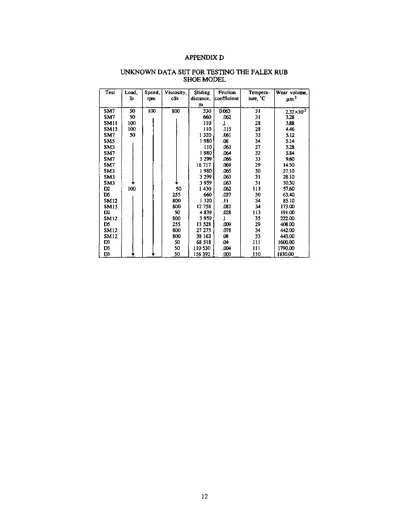
The first model investigated was the rub shoe model. The input variables used in the network included the following: load (lb). test time (min). sliding distance (m). viscosity (cSt). friction coefficient. and temper­ature eC). The defined output variable was the cumulative wear volume (mm3X 10-5). The values for wear volume were reduced from their actual values to make them more manageable. By using only these input and output variables. a data set containing 55 data points was accumulated. Also. a separate data set. with 26 data points. was developed and used as an unknown test set for the trained model.

By means of the neural network software. the training data set was broken up further into a training set (43 points) and a test set (12 points). This was done because the software trains the network on the training set. and. after each iteration through the data. tests itself on the test set. Thus, the network is exposed to all 55 data points during the training procedure. When the errors (actual output value-network approximation output value) from the test set were minimized, the network was instructed to stop training.

The default settings for the network design parameters were used. and the various architecture designs were studied to determine which design best suited this tribological data. The results from this analysis are shown in table II. The architectural design column represents the different designs available in the commercial software package. The R2-coefficient values presented illustrate each model's ability to approximate the outputs using only the default parameters.

The general regression architecture led to a model with the least amount of error in the training data. but the network did not have adequate generalized approximation abilities. This was due to the fact that this particular architecture (given the small number of data points available) may have been memorizing the data rather than learning it. This occurred with each of the three models developed in this study. Thus, unless large data sets can be developed. the general regression architecture does not appear to be a viable model. As a result. the input layer dampened recurrent network architectural design was selected as the architecture that best approximated the rub shoe data. Figure 3 schematically illustrates this architecture.

By using this architecture. with the default design parameters as a baseline. variations to the design parameters were investigated. These variations included the scaling function, the activation function. and the link parameters. Each parameter was systematically modified and the effect of each modification was again determined from the R2-coefficient of the networks approximation of the actual data. When all of the possible modifications were made to the architecture. the R2-coefficients were reviewed and the parameters yielding the highest R2 values were deemed "optimum."

4

For the rub shoe model, an "optimum" design consisting of a linear [0,1] scaling function, 10 neurons in the hidden layer, and a hyperbolic tangent activation (transfer) function for both the hidden layer and the output layer was determined. Modifications to learning rate, momentum, and initial weights did not signifi­cantly impact the ability of the model to approximate data. Thus, these variables were kept at their default levels. The parameters for the "optimum" architecture were used to train the network on the given input data. By going through an iteration process (backpropagation training algorithm), the weight of each neuron was modified until the network approximation error of the output value was minimized.

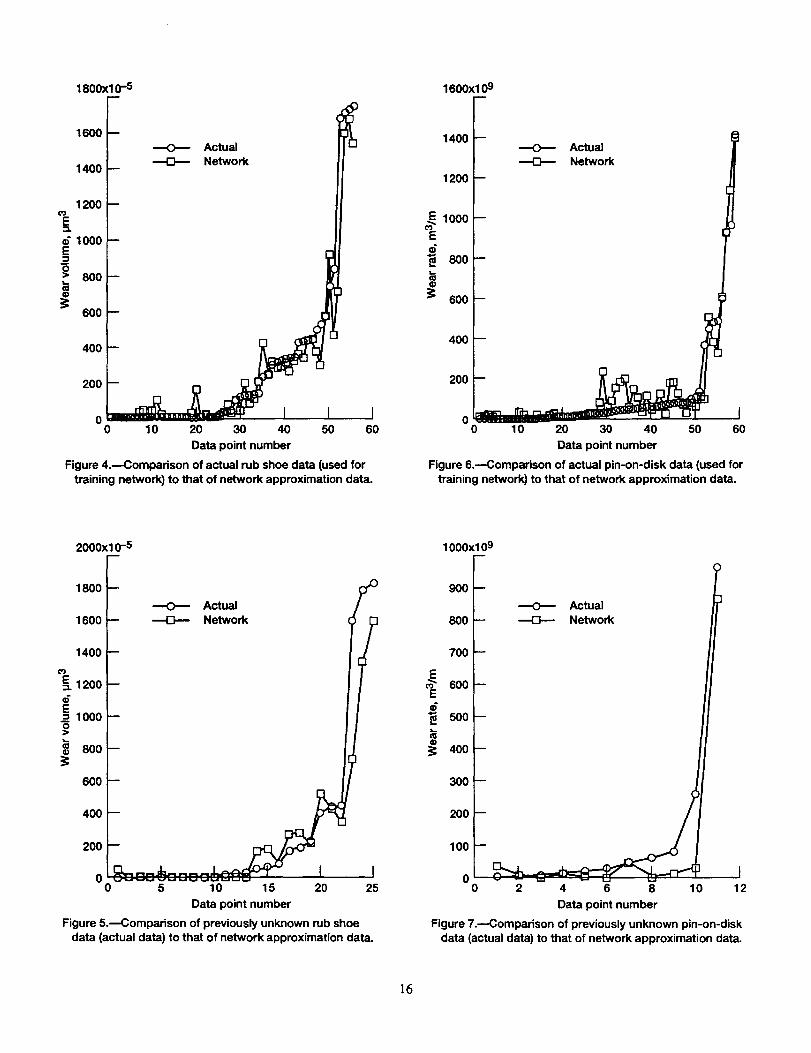
The result of training the network is shown graphically in figure 4, which illustrates the ability of the network to predict an output value when that value is included in the data set. Once the "optimum" design was trained, the model was applied to the unknown data set and told to approximate the output value. This analysis is shown graphically in figure 5, which illustrates the ability of the network to approximate the output when no output values were given in the data set and when the model had never seen the input values. The x-axis in these figures represents the number of the data point from the data set used to approximate the wear volume (y-axis). In other words, the range of the x-axis is the size of the data set used to test or train the model. The scatter observed in this model is indicative of the problems associated with using wear volume as the output parameter, namely the lack of repeatability from sample to sample. However, further nonlinear curve-fitting of the network approximation curve will generate a better approximation of the data being modeled.

Pin-on-Disk Model

The next data set investigated was that taken from pin-on-disk testing. These tests used several fluids as lubricants and various materials as pin/disk specimens. The inputs used for this model were similar to those in the previous model (i.e., load (N), speed (rn/s), viscosity (cSt), sliding distance (m), friction coefficient, and temperature (0C)), but the output variable was the wear rate (in units of m3/m (X 109)). The wear rate values were increased to a value greater than 1 was so that accurate R2-coefficients could be obtained to classify the architecture designs.

A similar procedure to the one discussed earlier in determining the proper design was followed for the pin-on-disk data. Table II presents the results from this analysis. As was the case with modell, the input layer dampened feedback network resulted in the best approximation of the training and test data. Using this basic design, the various design parameters were systematically modified to fully "optimize" the model. This optimum network consisted of a linear [-1,1] scaling function, 10 neurons in the hidden layer, and a logistical activation (transfer) function for the hidden and output layers. The default settings for learning rate (0.1), momentum (0.1), and initial weight (0.3) were used since modifications to these parameters tended to deteriorate the models ability to approximate outputs. Figures 6 and 7 illustrate graphically the networks ability to approximate wear rate for the training data set and test data set, respectively. An explanation for these figures is similar to that given for the rub shoe model.

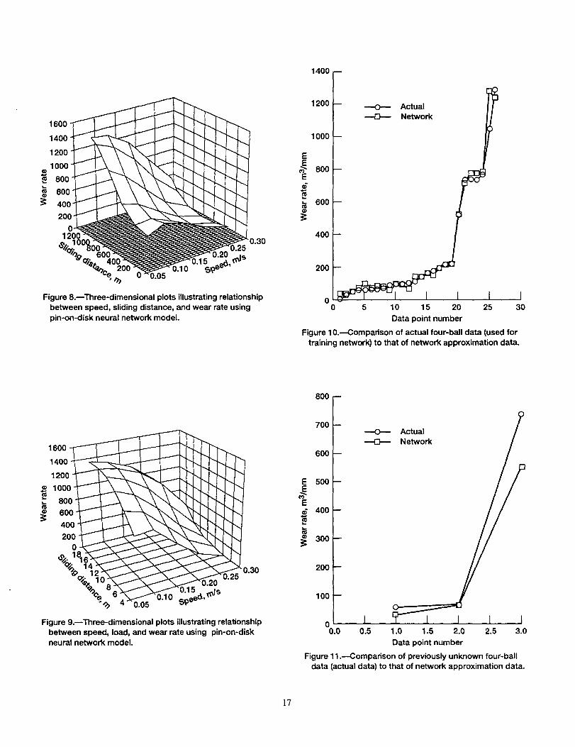
As mentioned previously, this commercial software package allows the contribution strengths for each input variable to be determined. Table III lists the contribution strengths for the input variables used in the pin­on-disk model. This indicates that of the six input variables used to develop this model, the sliding speed and the sliding distance are the most important inputs, while the friction coefficient and the temperature of the system are the least influential. The remaining variables, load and viscosity, are intermediate in value. For the sake of this study, though, these variables will be considered to be important.

Since it was known which variables were influential in predicting the desired output, the pin-on-disk model was then used to study the feasibility of using neural networks to extrapolate variables and determine their overall impact on wear rate. For this work, a new data set was generated "hypothetically." Constant values were used for the least influential variables, while the other input variables were allowed to vary over a large range of potential values. This means that the model has to interpolate or extrapolate between known inputs in order to obtain an approximated wear rate. The test matrix for this data set is shown in Table IV. No output variable was associated with these input values. The data set was then exposed to the network model so that wear rates could be approximated. The results of this analysis, shown in terms of three-dimensional surface plots in figures 8 and 9, illustrate the power of the neural network. As can be seen, the impact of each variable on the wear rate is clearly evident. As the sliding distance and load increase, the expected wear rate also increases. Simultaneously, as the speed of the system decreases, the expected wear rate will increase. This type of information would be extremely beneficial to the design engineer developing new bearing systems. Knowing what the needed specifications are, the design engineer could customize the materials, and

5

so forth to fit the system. This type of analysis could also steer the research engineer away from testing conditions which would be expected to lead to results outside of design specifications.

Four-Ball Data Model

A similar procedure to the one discussed earlier for the rub shoe data (for determining the proper design) was followed for the four-ball data. Table II presents the results from this analysis. Again, the input dampened feedback layer led to the most accurate model for this data set. The design specifications used to optimize the model included a linear [-1,11 scaling function, 20 neurons in the hidden layer, and a hyperbolic tangent activation (transfer) function in the hidden and output layers. Default values for learning rate, momentum, and initial weight were used. Figures 10 and 11 illustrate graphically the networks ability to approximate wear rates for the four-ball training data set and the test data set, respectively. Again it is seen that the neural network generated data can be made to very closely approximate the training data set, and then once trained the network can be used to predict data that it had not previously seen (the unknown test data). It is believed that an even better data fit could have been obtained if more data had been available to train the network.

CONCLUSIONS

The following results were obtained from this study: I. Neural networks have been shown to model simple mechanical systems illustrating the feasibility of

using neural networks to perform accelerated life testing on more complicated mechanical systems (i.e., bearings, etc.).

2. Although at an early stage of research, models have been successfully developed for three different test rigs (1) a rub shoe rig, (2) a pin-on-disk rig, and (3) a four-ball rig.

3. The models discussed have been shown to be capable of predicting wear rates regardless of the lubricants (materials) used in the system. This indicates that these models are able to generalize over a large range of variables.

4. The models have been shown to extrapolate/interpolate input variables to approximate wear rate values for conditions that have not been run experimentally.

5. An input layer dampened recurrent network architecture appeared to be the best architecture available (of those studied) to model wear data. Linear scaling functions and either hyperbolic tangent or logistic activation functions were beneficial.

REFERENCES

1. Kannel, J.W.; and Dufrane, K.F.: Rolling Element Bearings in Space. The 20th Aerospace Mechanisms Symposium, NASA CP-2423, 1986, pp. 121-132.

2. Zaretsky, E.V.: Liquid Lubrication in Space. NASA RP-1240, 1990. 3. Fusaro, R.L.: Tribology Needs for Future Space and Aeronautical Systems. NASA TM-I04525, 1991. 4. Fusaro, R.L.: GovernmentlIndustry Response to Questionnaire on Space Mechanisms/Tribology Technology

Needs. NASA TM-I04358, 1991. 5. Fusaro, R.L.: Space Mechanisms Needs for Future NASA Long Duration Space Missions. NASA

TM-105204, 1991. 6. Shapiro, W., et al.: Space Mechanisms Lessons Learned Study; Volume I-Summary. NASA TM-I07046.

1995. 7. Fleishchauer, P.D.; and Hilton. M.R.: Assessment of the Tribological Requirements of Advanced

Spacecraft Mechanisms. Proceedings of the Symposium on New Materials Approaches to Tribology: Theory and Applications. Materials Research Society, Pittsburgh, PA, 1989, pp. 9-20.

8. Miyoshi, K.; and Pepper, S.V.: Properties Data for Opening the Galileo's Partially Unfurled Main Antenna. NASA TM-105355, 1992.

9. Hebb. D.O.: The Organization of Behavior: A Neuropsychological Theory. Wiley, New York, 1949. 10. Lawrence, I.: Introduction to Neural Networks. Third ed., California Scientific Software, Grass Valley,

California. 1991. 11. Werbos, P.I.: Beyond Regression: New Tools for Prediction and Analysis in the Behavioral Sciences.

Ph.D. Thesis. Harvard University, 1975.

6

12. Wasserman, P.D.: Neural Computing: Theory and Practice. Van Nostrand Reinhold, New York, 1989. 13. Hady, W.F.; Johnson, R.L.; and Jones, W.R.: Friction and Wear of Poly(amide-imide), Poly imide, and

Pyrrone Polymers at 260C (5ooF) in Dry Air. NASA TN 0-6353, 1971. 14. Loomis, W.R.; and Jones, W.R. Jr.: Steady-State Wear and Friction in Boundary Lubrication Studies.

NASA TP-1658, 1980. 15. Jones, W.R.; and Ferrante, J.: Tribological Characteristics of Nitrogen (N+) Implanted Iron. NASA

TM-82839, 1992. 16. Hady, W.F.; and Jones, W.R.: Boundary Lubrication and Thermal Stability Studies With Five Liquid

Lubricants in Nitrogen to 400c. NASA TN D-6251, 1971. 17. Jones, W.R., Jr.; and Hady, W.F.: Boundary Lubrication of Formulated C-Ether in Air to 300 °C, 1. Phospho­

rous Ester Additives. NASA TN 0-6915. 1972. 18. Masuko, M.; et al.: A Vacuum Four-Ball Tribometer to Evaluate Liquid Lubricants for Space Applications.

NASA TM-I06264. 1993. 19. Masuko. M.; Jones.W.R.. Jr.; and Helmick. L.S.: Tribological Characteristics of Perfluoropolyether Liquid

Lubricants Under Sliding Conditions in High Vacuum. NASA TM-I06257. 1993.

TABLE I -DESIGN PARAMETERS AND V ALVES USED IN NEURAL NETWORK MODELS

Rub shoe rig Pin-on-disk rig Four-ball ri1;

Variable Value Variable Value Variable Value

Lubricants

PFPE (Type K) ------- Super-refined mineral oil ------- PFPE(~K) -------PFPE (Type F) ------- Ester-based fluids ------- PFPE (Type F) -------

n-Hexadecane ------- PFPE (lJ'Q.e D) -------Synthetic paraffinic oil -------

Glycol derivative -------Modified polyphenyl ether -------

Inputs

Load.lb 50 to 100 Load. kg 0.5 to 1.5 Pressure-viscosity -------coefficient

Viscosity. cSt 50 to 800 Speed, mlmin 2.6 to 18.2 Transient friction -------Sliding distance. 50 to 25 000 Sliding distance. m 100 to 1200 Initial A ratio -------m

Friction 0.05 to 0.20 Temperature. °C 25 to 400 Kinematic viscosity. 250 to 800 coefficient cSt

Temperature, QC 25 to 115 Friction coefficient -0.1 to 0.2 Molecular weight 5600 to 10000

Kinematic viscosity. cSt 0.5 to 40 Vapor pressure. torr 3 to 500 OOOxlo-12

Surface tension. 18to 25 c!i'neslcm

Viscosity index 134 to 355

Load. N 200 to 600

Sliding distance. m 350 to 525

Output

Wear volume ------- Wear rate -- ----- Wear rate -------

7

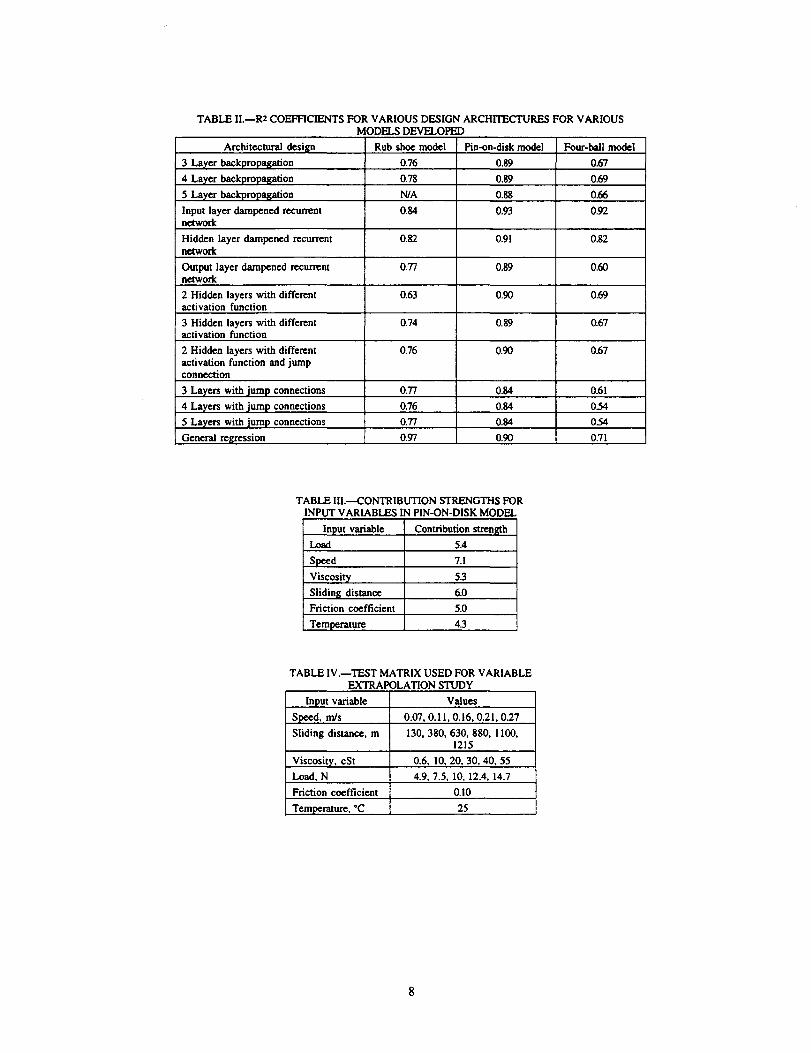
TABLE 1I.-R2 COEFFICIENTS FOR VARIOUS DESIGN ARCHITECTURES FOR VARIOUS MODELS DEVELOPED

Architectural desiltll Rub shoe model Pin-on-disk model

3 Layer backpropagation 0.76 0.89

4 Layer backpropall;ation 0.78 0.89

5 Layer backpropagation NJA 0.88

Input layer dampened recurrent 0.84 0.93 network

Hidden layer dampened recurrent 0.82 0.91 network

Output layer dampened recurrent 0.77 0.89 network

2 Hidden layers with different 0.63 0.90 acti vation function

3 Hidden layers with different 0.74 0.89 activation function

2 Hidden layers with different 0.76 0.90 activation function and jump connection

3 Layers withiump connections 0.77 0.84

4 Layers with jump connections 0.76 0.84

5 Layers with jump connections 0.77 0.84

General rell;ression 0.97 0.90

TABLE lll.-CONTRIBUTION STRENGTHS FOR INPUT V ARlABLES IN PIN-ON-DISK MODEL

Input variable Contribution strength

Load 5.4

~d 7.1

Viscosity 53

Sliding distance 6.0

Friction coefficient 5.0

Temperature 43

TABLE IV.-TEST MATRIX USED FOR VARIABLE EXTRAPOLATION STUDY

Input variable Values

Speed. mls 0.07.0.11.0.16.0.21.0.27

Sliding distance. m 130.380.630.880. 1100. 1215

Viscosity. cSt 0.6. 10.20.30.40.55

Load. N 4.9.7.5. 10. 12.4. 14.7

Friction coefficient 0.10

Temj>erature. ·C 25

8

Four-ball model

0.67

0.69

0.66

0.92

0.82

0.60

0.69

0.67

0.67

0.61

0.54

0.54

0.71

APPENDIX A

DATA SET FOR TIlE FALEX RUB SHOE MODEL

Test Load. Speed. Viscosity, Sliding Friction Temperature, Wear Ib rpm cSt distance. coefficient ·C Volume.~

m

SM-5 50 100 800 330 0.056 30 2.9xlO·s

SM-5

I 660 .059 30 3.32

SM-5 1320 .057 33 3.5 SM-4 llO .044 26 3.54 SM-4 330 .047 29 3.56 SM-3 330 .062 30 5.94 SM-13 100 440 .117 34 6.74 SM-ll 100 550 .11 33 8 SM-4 50 660 .047 31 8.02 SM-12 100 110 .II 27 8.16 SM-II 100 11768 .1 36 9.46 SM-ll 100 40 583 .11 36 10 SM-6 50 330 .076 30 10.3 SM-5

j 3299 .059 34 10.6

SM-6 660 .079 32 13.7 SM-4 1320 .05 33 13.8 SM-6 1320 .058 32 15.1 SM-3 660 .063 32 15.4 SM-13 100 880 .119 38 16.1 D2 100 50 220 .047 ll4 16.7 SM-5 50 800 47841 .129 31 18.2 SM-12 100

I 330 .12 31 18.4

SM-4 50 1980 .055 33 19.5 SM-6 50 1980 .072 31 23.6 SM-4 50 5279 .05 34 34.5 SM-12 100 660 .12 33 36.1 05 100 255 330 .039 29 37.1 SM4 50 800 21886 .044 34 47 05 100 255 1320 .026 29 113 SM-12 800 1980 .11 34 124 02 50 3189 .043 ll2 139 SM-12 800 2640 .1 33 140 05 255 1980 .022 29 143 03 50 1210 .094 114 146 02 50 6709 .033 III 242 03 50 2420 .084 113 248 SM-12 800 6379 .07 32 302 03 50 4619 .075 113 318 SM-12 800 7809 .08 34 328 SM-12

I 9238 .075 34 343

SM-12 11218 .085 34 348 SM-12 12978 .075 35 350 SM-12 23756 .06 33 437 SM-12 25625 .085 35 439 SM-12 42012 .065 36 449 SM-12 100 852 .07 32 451 02 50 17 047 .06 ll2 507 D3 50 8798 .063 113 533 05 255 58509 .006 28 579 03 50 19247 .015 108 754 D3

I 22436 .034 III 849

03 86 .028 113 1690 03 83 .009 109 1720 03 ll4 0 110 1740 03 97 .012 III 1760

9

APPENDIXB

DATA SET FOR THE PIN-ON-DISK MODEL

Test Load, Speed, Viscosity, Sliding Friction Temperature, Wear rate, N mls cSt distance, coefficient ·C m3/m

m

NASA TN 0-6251 9.8 0.272 0.685 980 0.12 300 1.02 x 109

NASA TN 0-6251

I 6

I .12 200 1.02

NASA TN 0-6251 6 .12 200 2.04 NASA TN 0-6251 .94 .13 250 3.07 NASA TN 0-6251 1.75 .1 250 3.07 NASA TN 0-6251 1.38 .14 400 3.07 NASA TN 0-6251 1.7 .14 350 4.09 NASA TN 0-6251 1.225 .08 300 4.09 NASA TN 0-6915 .2702 40 425 .12 25 4.4 NASA TN 0-6251 .272 .935 980 .Q7 350 5.11 NASA TN 0-6251

1 .73

1 .06 400 6.13

NASA TN 0-6251 1.38 .14 400 6.\3 NASA TN 0-6251 3.5 .12 250 9.2 NASA TN 0-6915 .2702 .69 425 .12 300 9.41 NASA TN 0-6353 14.7 .17 .56 250 .16 260 10 NASA TN 0-6251 9.8 .272 1.38 980 .14 200 10.2 NASA TN 0-6251 .272 4.9 980 .1 1 12 NASA TN 0-6915 .2702 1.27 425 .2 12.3 NASA TN 0-6915 .2702 1.27 425 .18 14.7 NASA TND-6915 .2702 4.5 425 .16 100 18.2 NASA TN 0-6251 .272 1.7 980 .14 350 20.5 NASA TN 0-6915 .2702 4.5 425 .14 100 21.2 NASA TN 0-6915

1 4.5

1 .16 100 22.4

NASA TN 0-6915 4.5 .15 100 22.9 NASA TN 0-6915 40 .1 25 29.4 NASA TN 0-6251 .272 2.8 980 .11 250 30.6 NASA TN 0-6915 .2702 40 425 .I 25 32.3 NASA TN 0-6915 .2702 40 425 .09 25 35.3 NASA TM-82839 4.9 .075 4.31 145 .15 20 37 NASA TN 0-6915 9.8 .2702 .69 425 .16 300 37 NASA TM-82839 4.9 .073 4.31 142 .15 20 40 NASA TM-82839

1 .069

1 144

1 1 44

NASA TM-82839 .073 141 49 NASA TM-82839 .075 155 50 NASA TN 0-6251 9.8 .272 3.5 980 .12 250 51.1 NASA TM-82839 4.9 .071 4.31 138 .15 20 53 NASA TM-82839 4.9 .078 4.31 149 .16 20 57 NASA TN 0-6251 9.8 .272 1.3 980 .12 350 61.3 NASA TM-82839 4.9 .07 4.31 138 .15 20 62 NASA TN 0-6915 9.8 .2702 .69 425 .2 300 64.7 NASA TM-82839 4.9 .074 4.31 143 .15 20 66 NASA TN 0-6251 9.8 .272 2.38 980 .13 300 71.6 NASA TM-82839 4.9 .071 4.31 134 .14 20 75 NASA TM-82839 4.9 .067 4.31 134 .15 20 80 NASA TN 0-6915 9.8 .2702 55 425 .1 25 82.4 NASA TN 0-6915 9.8 .2702 .68 425 .12 300 82.4 NASA TN 0-6915 9.8 .2702 1.33 425 .16 200 82.4 NASA TN 0-6353 14.7 .17 .56 250 .13 260 100 NASA TM-82839 4.9 .071 4.31 141 .15 20 110 NASA TM-82839

I .078 4.3097 152 .15 25 137.2

NASA TM-82839 .075 4.3097 146 .16 25 367.5 NASA TP-1658 .2702 39.6 1125 .09 20 453 NASA TM-82839 .072 4.3097 151 .14 25 485.1 NASA TM-82839 .077 4.3097 154 .14 25 490 NASA TP-1658 .2027 39.6 1100 .09 20 597 NASA TP-1658 .1352 1 920

1 1 927

NASA TP-1658 9.8 .2702 1125 964 NASA TP-1658 9.8 .2027 1215 1421

10

APPENDIXC

DATA SET FOR THE FOUR-BALL MODEL

Test Lubricant Pressure- Transient Initial A- Kinetic Molecular Vapor Surface Viscosity Load, Sliding Sliding Wear rate, viscosity friction ratios viscosity, weight pressure, tension, index N speed, distance, mm 3/mm

coefficient, cSt torr dynes/em mls mm (l

I Krytox 143 AC 4.50E-08 0 2 800 6250 8.00E-08 18 134 200 0.0288 475200 9xl01l

2 Krytox 143 AC 4.50E-08 0 2 800 6250 8.00E-08 18 134 200 501120 26 3 Krytox 143 AC 4.50E-08 0 2 800 6250 8.00E-08 18 134 200 528768 66 4 Fomblin Z25 1.50E-08 I I 255 10000 2.90E-12 25 355 600 466 560 67 5 Fomblin Z25 1.50E-08 I 1 255 10000 2.90E-12 25 355 600 466560 69 6 Krytox 143 AC 4.50E-08 0 2 800 6250 8.00E-08 18 134 200 451008 71 7 Krytox 143 AC 4.50E-08 0 2 800 6250 8.00E-08 18 134

1 473472 88

8 Demnum 2.6OE-08 2 13 250 5600 5.00E-07 18.5 200 362880 96 9 Fomblin Z25 1.50E-08 I

I 255 10000 2.90E-12 25 355 362880 98

10

I I j I I I I I 600 466560 106

11 200 362880 III 12

1 466560 142

13 466560 160 14 366 336 179 15 Demnum 2.6OE-08 2 13 250 5600 5.00E-07 18.5 200 600 362880 197 16 Demnum 2.6OE-08 2 13 250 5600 5.00E-07 18.5 200

I 371520 216

17 Demnum 2.6OE-08 2 13 250 5600 5.00E-07 18.5 200 466560 221 18 Krytox 143 AC 4.50E-08 0 2 800 6250 8.00E-08 18 134 435456 521 19

1 1 1 1 1 1 1 1 1 468288 740

20 470016 742 21 468288 770 22 Fomblin Z25 1.50E-08 I I 255 10000 2.90E-12 25 355 200 499392 1049 23 Fomblin Z25 1.50E-08 I 1 255 10000 2.90E-12 25 355 200 475200 1290

Test

SM7 SM7 SMII SMI3 SM7 SM5 SM3 SM7 SM7 SM7 SM3 SM3 SM3 D2 D5 SMI2 SM13 D2 SMI2 D5 SMI2 SMI2 D3 D3 D3

APPENDIXD

UNKNOWN DATA SET FOR TESTING THE FALEX RUB SHOE MODEL

Load, Speed, Viscosity, Sliding Friction Tempera- Wear volume, lb rpm cSt distance, coefficient ture, 'C ~m3

m 50 100 800 330 0.063 31 232xI0's 50 660 .062 31 328

100 110 .I 28 3.88 100 110 .115 28 4.46 50 1320 .061 33 5.12

1980 .06 34 5.14 110 .063 27 528

1980 .064 32 5.84 3299 .066 33 9.60

16717 .069 29 14.50 1980 .065 30 27.10 3299 .063 31 28.10 3959 .063 31 30.30

100 50 1430 .062 \13 57.6IJ 255 660 .037 30 63.40 800 1320 .il 34 85.10 800 12758 .082 34 173.00 50 4839 .028 113 191.00

800 3959 .1 35 222.00 255 13528 .009 29 408.00 800 27275 .078 34 442.00 800 38163 .08 33 443.00 50 68518 .04 III 1600.00 50 110530 .004 III 1790.00 50 156392 .003 110 1830.00

12

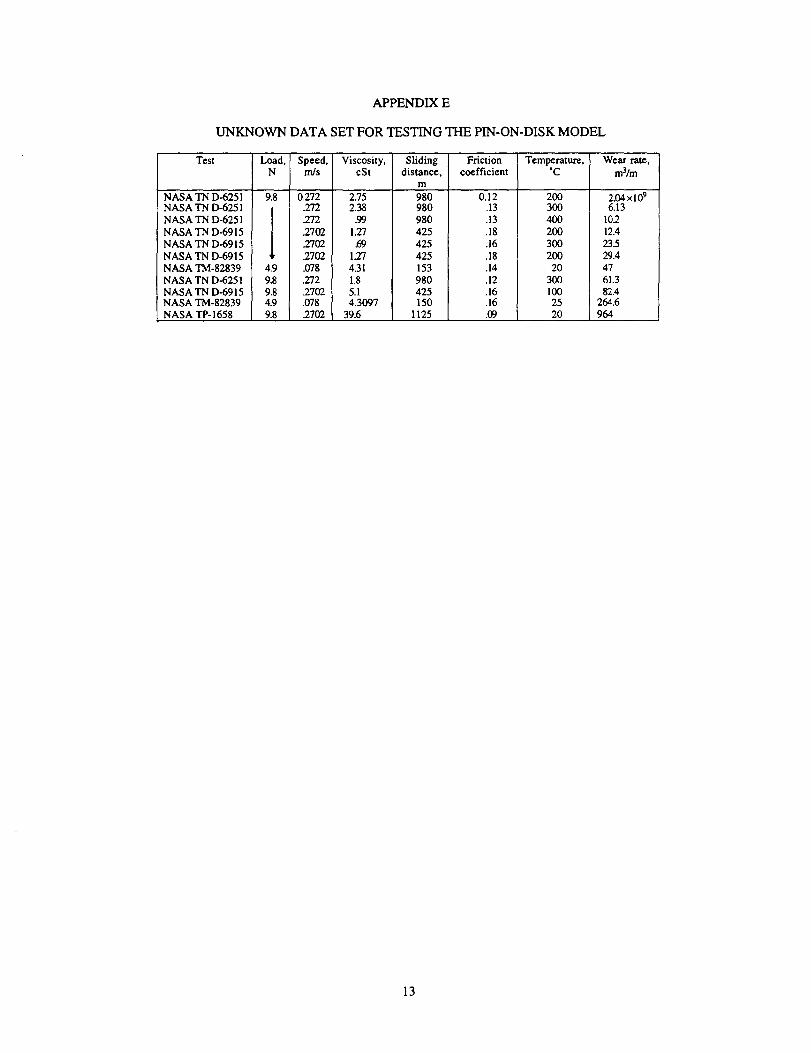
APPENDIXE

UNKNOWN DATA SET FOR TESTING TIlE PIN-ON-DISK MODEL

Test Load, Speed, Viscosity, Sliding Friction Temperature, Wear rate, N mls cSt distance, coefficient ·C m3/m

m NASA TN 0-6251 9.8 0.272 2.75 980 0.12 200 2.04xl09 NASA TN 0-6251

1 .272 2.38 980 .13 300 6.13

NASA TN 0-6251 .272 .r:yj 980 .13 400 10.2 NASA TN 0-6915 .27m 1.27 425 .18 200 12.4 NASA TN 0-6915 .27m .69 425 .16 300 235 NASA TN 0-6915 .27m 1.27 425 .18 200 29.4 NASA TM-82839 4.9 .(J78 4.31 153 .14 20 47 NASA TN 0-6251 9.8 .272 1.8 980 .12 300 61.3 NASA TN 0-6915 9.8 .27m 5.1 425 .16 100 82.4 NASA TM-82839 4.9 .CJ78 4.3097 150 .16 25 264.6 NASA TP-1658 9.8 .27m 39.6 1125 JE 20 964

13

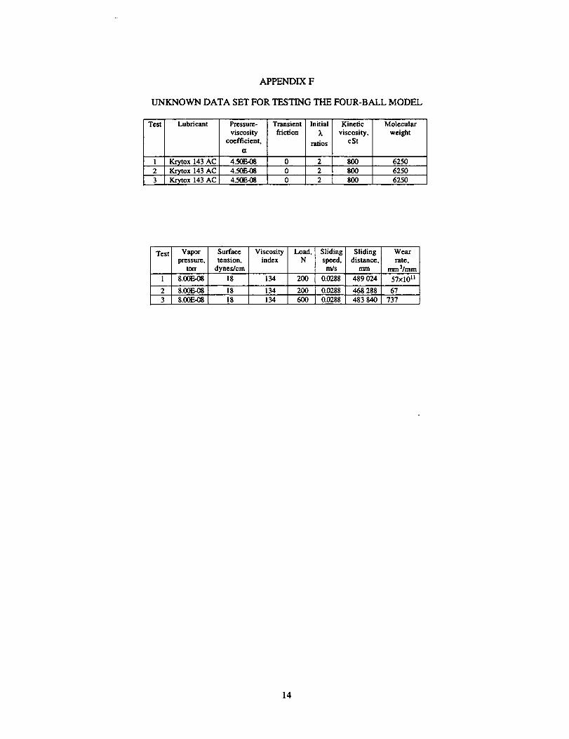
APPENDIXF

UNKNOWN DATA SET FOR TESTING THE FOUR-BALL MODEL

Test Lubricant Pressure- Transient Initial Kinetic Molecular viscosity friction A viscosity, weight

coefficient. ratios cSt a

1 Krytox 143 AC 4.50&08 0 2 800 6250 2 Krytox 143 AC 4.50E-08 0 2 800 6250 3 Krytox 143 AC 4.50E-08 0 2 800 6250

Test Vapor Surface Viscosity Load. Sliding Sliding Wear pressure, tension, index N speed. distance. rate.

torr dynes/cm mJs mm mm 3/mm 1 8.00E-08 18 134 200 0.0288 489024 57xlOli

2 8.00&08 18 134 200 0.0288 468288 67 3 8.00E-08 18 134 600 0.0288 483840 737

14

~ Weights Data manipulation Outputs

I Artificial neuron I Figure 1.-Artificial neuron with activation function (Ref.5).

Wear track """\ \

(b)

I I

... -- Rider slanted ... at 45° to disk

Applied load

rotation

Inputs

I Hidden I I Outputs I

Figure 3.-5chematic illustration of the input layer dampened recurrent feedback design architecture.

cup

Flex

(c)

Rotating ball

/r- Stationary balls

Figure 2.-5chematic diagrams of rub shoe sliding specimens, pin-on-disk sliding specimens, four-ball sliding specimens. (a) Rub shoe. (b) Pin-on-disk. (c) Four-ball.

15

1800x1o-S

1600

1400

1200 (')

E :::l.

a; 1000 E ::l g ... 800

~ 600

400

200

~ Actual -0- Network

10 20 30 40 Data point number

50 60

Figure 4.-Comparison of actual rub shoe data (used for training network) to that of network approximation data.

2000x1o-S

1800

1600

1400 (')

§. 1200 tD

§ 1000 g ~ 800

600

400

200

~ Actual -0- Network

5 10 15 Data point number

20 25

Figure 5.-Comparison of previously unknown rub shoe data (actual data) to that of network approximation data

16

1600x109

1400

1200

~ 1000 (')

E

~ 800

~ 600

~ Actual -0- Network

Data point number

Figure 6.-Comparison of actual pin-on-disk data (used for training network) to that of network approximation data.

1000x109

900

800

700

J. 600 E a; ~ 500

~ 400

300

~ Actual -0- Network

Data point number

Figure 7.-Comparison of previously unknown pin-on-disk data (actual data) to that of network approximation data.

Q)

1600

1400

1200

1000

~ 800 "-III 600

~ 400

Figure 8.-Three-dimensional plots illustrating relationship between speed, sliding distance, and wear rate using pin-an-disk neural network model.

1600

1400

1200

~ 1000

lu 800

~ 600 400

200 o

.n 18 u~. 16

0;->. 14 ~ 12

o;,pl; 10 ~Cl 8 6 \9

'''» 4 0.05

0.20 0.15 ("('Is S9eeO'

0.30 0.25

Figure 9.-Three-dimensional plots illustrating relationship between speed, load, and wear rate using pin-an-disk neural network model.

17

1400

1200

1000

E

J. 800 E

400

200

--0- Actual -0- Network

o~=-~----~----J-----L---~----~

o 5 10 15 20 25 30 Data point number

Figure 10.-Comparison of actual four-ball data (used for training network) to that of network approximation data.

800

700 ---0-- Actual -0- Network

600

E 500

J. E GS 400 ~ "-III Q) 300 ~

200

100

OL...----..L-----'------'------L-----I.----~

0.0 0.5 1.0 1.5 2.0 2.5 3.0 Data point number

Figure 11.-Comparison of previously unknown four-ball data (actual data) to that of network approximation data.

REPORT DOCUMENTATION PAGE Form Approved

OMB No. 0704-0188 Public reporting burden .or !his collection 01 information is estimated to average 1 hour per response. including the time lor reviewing instructions. searching existing data S0UfC8S. gathering and maintaining the data needed. and completing and raYiewing the collection 0' informalion. Send comments regarding lIIis burden estimate or any other aspect 0' !his collection 0' information, including suggestions 'or ,edUCing !his burd8n, to Washington Headquarters Services, Directorata lor Information Operations and Reports, 1215 Jefferson Davis Highway, Su~e 1204, Arlington, VA 22202·4302. and to the Office 01 Management and Budget, Paperwork Reduction Project (0704-0188), Washington, DC 20503.

1. AGENCY USE ONLY (Leave blank) 12. REPORT DATE r' REPORT TYPE AND DATES COVERED

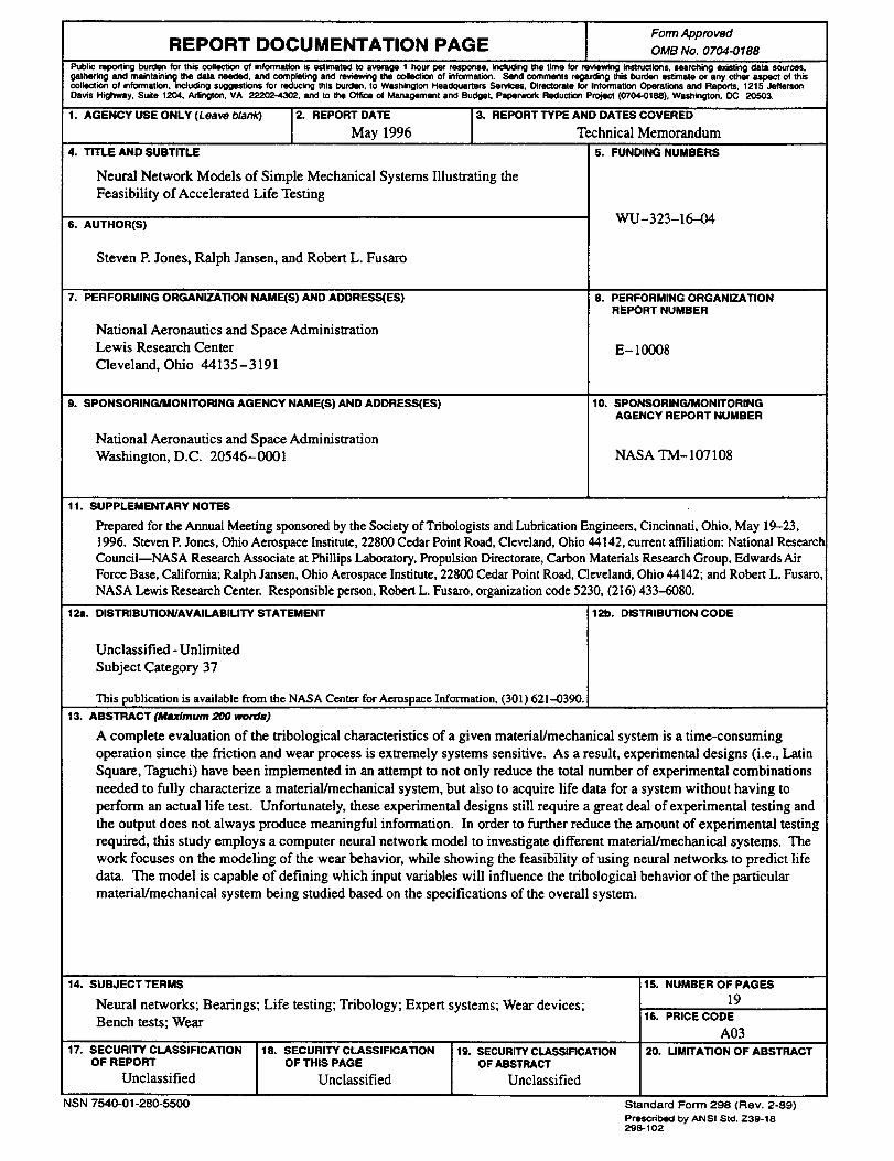
May 1996 Technical Memorandum 4. TITLE AND SUBTITLE 5. FUNDING NUMBERS

Neural Network Models of Simple Mechanical Systems Illustrating the Feasibility of Accelerated Life Testing

6. AUTHOR(S) WU-323-16-04

Steven P. Jones, Ralph Jansen, and Robert L. Fusaro

7. PERFORMING ORGANIZATION NAME(S) AND ADDRESSCES) 8. PERFORMING ORGANIZATION REPORT NUMBER

National Aeronautics and Space Administration Lewis Research Center E-lOOO8 Cleveland, Ohio 44135-3191

9. SPONSORINGIMONITORING AGENCY NAME(S) AND ADDRESSCES) 10. SPONSORINGIMONITORING AGENCY REPORT NUMBER

National Aeronautics and Space Administration Washington, D.C. 20546-0001 NASA TM-l 07108

11. SUPPLEMENTARY NOTES

Prepared for the Annual Meeting sponsored by the Society of Tribologists and Lubrication Engineers, Cincinnati, Ohio, May 19-23, 1996. Steven P. Jones, Ohio Aerospace Institute, 22800 Cedar Point Road, Cleveland, Ohio 44142, current affiliation: National Research Council-NASA Research Associate at Phillips Laboratory, Propulsion Directorate, Carbon Materials Research Group, Edwards Air Force Base, California; Ralph Jansen, Ohio Aerospace Institute, 22800 Cedar Point Road, Cleveland, Ohio 44142; and Robert L. Fusaro, NASA Lewis Research Center. Responsible person, Robert L. Fusaro, organization code 5230, (216) 433-6080.

12 •• DISTRIBUTION/AVAILABILITY STATEMENT 12b. DISTRIBUTION CODE

Unclassified - Unlimited Subject Category 37

This publication is available from the NASA Center for Aerospace Information, (301) 621~390. 13. ABSTRACT (IAn/mum 200 words)

A complete evaluation of the tribological characteristics of a given material/mechanical system is a time-consuming operation since the friction and wear process is extremely systems sensitive. As a result, experimental designs (i.e., Latin Square, Taguchi) have been implemented in an attempt to not only reduce the total number of experimental combinations needed to fully characterize a material/mechanical system, but also to acquire life data for a system without having to perform an actual life test. Unfortunately, these experimental designs still require a great deal of experimental testing and the output does not always produce meaningful information. In order to further reduce the amount of experimental testing required, this study employs a computer neural network model to investigate different materiallmechanical systems. The work focuses on the modeling of the wear behavior, while showing the feasibility of using neural networks to predict life data, The model is capable of defining which input variables will influence the tribological behavior of the particular material/mechanical system being studied based on the specifications of the overall system.

14. SUB.lECT TERMS

Neural networks; Bearings; Life testing; Tribology; Expert systems; Wear devices; Bench tests; Wear

17. SECURITY CLASSIFICATION 18. SECURITY CLASSIFICATION 19. SECURITY CLASSlFlCAnON OF REPORT OF THIS PAGE OF ABSTRACT

Unclassified Unclassified Unclassified

NSN 7540-01-280·5500

15. NUMBER OF PAGES

19 16. PRICE CODE

A03 20. LIMITATION OF ABSTRACT

Standard Form 298 (Rev. 2-89) Prescribed by ANSI Std. Z39-1a 291H02