Embed Size (px)
Citation preview

Network Externalities in Collaborative Consumption:Theory, Experiment, and Empirical Investigation of Crowdfunding*
Zhuoxin Li
Carroll School of Management, Boston College
140 Commonwealth Ave, Fulton Hall 460, Chestnut Hill, Massachusetts 02467
Phone: (617) 552-2468, Email: [email protected]
Jason A. Duan
McCombs School of Business, The University of Texas at Austin
2110 Speedway Stop B6700, Austin, Texas, 78712
Phone: (512) 232-8323, Email: [email protected]
*The authors would like to thank the NET Institute (www.NETinst.org) for financial support ofthe project.

Network Externalities in Collaborative Consumption:Theory, Experiment, and Empirical Investigation of Crowdfunding
October 18, 2016
For most recent version, click here
Abstract: Crowdfunding is an emerging internet fundraising mechanism for soliciting capital from
the crowd to support entrepreneurial ventures. Entrepreneurs set a funding target and deadline,
and investors decide whether to contribute. Investors may estimate a project’s chance of funding
success not only from the amount of funding the project has attained, but also from the timing
that this number was achieved. To illustrate this, suppose there are two projects that are identical
except that one reaches 50% of its funding goal in 5 days whereas the other reaches this percentage
in 20 days (suppose the funding period for both projects is 30 days). The two projects have
attracted the same amount of funding, however, the temporal information (5 days vs. 20 days)
may also provide essential information for investors to evaluate a project’s prospect and its chance
of reaching the preset funding target by the fixed deadline. The temporal dynamics of network
externalities have not been well-understood in the literature.
This paper combines randomized experiments, theoretical modeling, and empirical methods
to investigate investors’ contribution behaviors in the presence of network externalities and a
deadline. The empirical model captures investors’ expectation on the prospect of a project based
on its current funding status and time progress. Model estimation shows that investors are more
likely to back a project that has already reached a critical mass of funding goal (positive network
externalities). For the same amount of achieved funding, the backing propensity declines over
time (negative time effects). These two opposing forces give rise to a critical mass of funding
the project must attain on time to achieve successful funding. Interestingly, this critical mass
changes over the funding period. Simulation studies show that projects may fail to attain the
critical mass due to unfavorable shocks at the early stage of the funding cycle. Our model and
results shed light on the temporal dynamics of network externalities in collaborative consumption
with a target and deadline. We provide actionable promotion strategies and decision support for
entrepreneurs to dynamically manage their crowdfunding campaign.
Keywords: crowdfunding; group buying; social media; entrepreneurship; network externality;herding; network effects; hazards model; Bayesian inference
1

1 Introduction
Crowdfunding is an emerging internet fundraising mechanism for soliciting capital from the online
crowd to support innovative projects. Facing the difficulties and costs of raising early-stage funding
from institutional investors (e.g., angel investors, banks, and venture capital funds), entrepreneurs
are tapping into the online communities of consumer investors (Economist 2010, Schwienbacher
and Larralde 2012). Crowdfunding platforms such as Kickstarter.com and IndieGoGo.com allow
entrepreneurs to request funding for clearly specified projects from a large number of individual
investors (also called “backers”), often vowing future products or certain forms of recognition in
return. Crowdfunding has helped new ventures to raise billions of dollars in total and the volume of
transactions continues increasing (Agrawal et al. 2013, Mollick 2014, Burtch et al. 2013). Legalized
by the Jumpstart Our Business Startups (JOBS) Act passed in April 2012, crowdfunding efforts
may give investors equity stakes in return for their funding in the future.
In contrast to traditional capital sourcing models such as venture capital, crowdfunding is
characterized by many small investors, collective evaluation of projects, and high transparency of
funding status. In addition to the project information provided by entrepreneurs, investors also
assess a project’s potential for success based on other investors’ investment decisions (Zhang and
Liu 2012). Besides, major crowdfunding platforms like Kickstarter require entrepreneurs to set a
funding target and deadline for any project. Entrepreneurs will receive the funding only if their
project successfully reaches the funding target by the deadline. In the presence of the funding
target and deadline, investors also assess the project’s prospect of success based on whether it can
quickly attract a critical mass of backers. Facing opportunity costs, investors often do not want to
contribute to a project that is unlikely to reach its funding goal. Strong network externalities are
critical to the success of a project in this context, because the larger amount of funding it attains
at the early stage of the funding cycle, the more likely the project will be able to attract more
backers and reach its funding goal by the deadline.
Despite its importance, the role of network externalities in the presence of a funding target
and deadline has been under explored in the literature. A major objective of this paper is to
demonstrate how time-varying network externalities and the deadline jointly give rise to a critical
mass of funding that a project must achieve on time. Investors may estimate a project’s chance of
2

success not only from the amount of funding the project has attained, but also from the timing that
this number was achieved. To illustrate this point, suppose there are two projects that are identical
except that one reaches 50% of its funding goal in 5 days whereas the other reaches this percentage
in 20 days (suppose the funding period for both projects is 30 days). Since the two projects have
attracted the same amount of funding, one would consider the two projects equally appealing if
the temporal information (5 days vs. 20 days) were not taken into account. However, the temporal
information actually provides essential information for investors to evaluate a project’s prospect and
its probability of receiving sufficient funding. The project reaching 50% of its funding goal within
5 days appears to be a better investment option, for attracting a large percent of funding goal in
a short time indicates the project’s good prospect of reaching the funding goal by the deadline.
Understanding network externalities under the constraint of a funding target/deadline is an
essential step towards deeper understanding of the online crowdfunding mechanism. The results
from this research also provide insights for other relevant business problems where agents coordinate
to achieve certain goal by a deadline. For instance, on group-buying platforms like Groupon.com,
sellers may offer products and services at discount prices on the condition that a minimum number
of buyers would make the purchase by the deadline. To our best knowledge, this is the first empirical
research that investigates the joint effects of time and network externalities in the setting of targets
and deadlines. Specifically, we aim to answer the following questions:
(1) How do investors form their expectations on the prospect of a project based on its current
funding status (e.g., percent of funding goal already achieved and the length of time left)?
(2) What are the promotion strategies entrepreneurs may use to increase the probability of
funding success?
Our model captures investors’ perceived success probability of a crowdfunding project. The
model estimates provide empirical evidence of how investors decide whether to contribute to a
project based on current funding performance and the progress in time. We find that investors
are more likely to back a project that has already attracted a critical mass of funding (positive
network externalities). When the achieved funding amount is fixed, investors’ backing propensity
declines over time as investors’ perceived success probability of a crowdfunding project decreases
over time (negative time effects). These two competing forces determine an investor’s overall
backing propensity and give rise to a critical mass which the funding the project needs to attain
3

on time in order to achieve successful funding by the deadline.
This research makes several contributions. Existing studies on network externalities have docu-
mented that the value of a product/service increases in its network size (see, e.g., Katz and Shapiro
1986, Katz and Shapiro 1992). We demonstrate that the presence of network externalities and
funding deadline jointly leads to a critical mass for funding success, and this critical mass changes
over time. We provide a parsimonious yet flexible framework for modeling investor decisions in
crowdfunding. Empirical results show that incorporating both network externalities and time ef-
fects significantly improves model fit. Ignoring either effect leads to biased parameter estimates.
This research contributes to the emerging literature on online crowdfunding. Several papers
have provided descriptive evidences on why people contribute to online crowdfunding. However,
existing studies have not formulated investors’ decision problem during the crowdfunding process.
This paper constructs an economic framework to understand dynamic investor behaviors and offers
an intuitive explanation for the time-varying funding patterns. We find that if the negative time
effects dominate the positive network externalities, investors become less likely to contribute to a
project in later periods. However, if the positive network externalities dominate, investors are more
likely to contribute in later periods. We demonstrate how the presence of network externalities
and funding deadline jointly leads to a critical mass for funding success, and how this critical mass
changes over time. Our results shed light on the complex crowdfunding process which has yet to
be unraveled to researchers and practitioners.
Our model and results provide important insights for entrepreneurs and crowdfunding platforms.
We demonstrate by counterfactual simulations that crowdfunding projects may fail to reach their
funding target due to low investor valuation. Advertising on various media to attract more potential
investors is a plausible means to achieve successful funding. We evaluate the impact of the timing
of the promotion strategy on crowdfunding performance and find that early promotion is more
effective. This is due to the direct effect and indirect effect of promotion. Promotion informs a
larger number of investors and thus more contributions (direct effect). In additional, a large amount
of funding achieved in early periods also boost the subsequent-arriving investors’ expectation on the
prospect of the project, which increases their backing propensity (indirect effect). As a result, the
project will continue to receive more contributions in later periods, even though the entrepreneur
has ceased promotion.
4

A highly interesting result from our simulation is that high-valuation projects may also fail to
attain the critical mass of funding and eventually fizzle out, due to a few unfavorable shocks in
investor arrivals at the early stage of the funding cycle. In the presence of network externalities,
negative shocks in early periods will carry over to later periods and have permanent negative effects
on the final crowdfunding outcome. We derive dynamic promotion strategies and provide decision
support for entrepreneurs to implement real-time control and management of their crowdfunding
projects.
The rest of the paper is organized as follows. In the next section, we elaborate on how our model
and results provide new insights into the literature on online crowdfunding, followed by some results
from an online experiment about crowdfunding in Section 3. We present details of our empirical
dataset and provide exploratory evidence on the interaction between network externalities and time
effects in Section 4. We then construct our model followed by its estimation method in Section
5. In Section 6, we present the estimation results and their interpretations, followed by the use
of counterfactual simulations for managerial analysis in Section 7. We conduct several robustness
checks in Section 8 and conclude the paper in Section 9.
2 Related Literature
Our research is related to the literature on product adoption subject to network externalities and
the literature on online crowdfunding and group buying. We discuss these two streams of literature
below.
Network Externalities and Critical Mass
Existing studies on network externalities have documented that the value of a product/service may
increase in its installed base (see, e.g., Katz and Shapiro 1986, Brynjolfsson and Kemerer 1996,
Kauffman et al. 2000). The larger the total number of buyers using compatible products, the greater
benefits each buyer receives (Katz and Shapiro 1992). The value of cross-side network externalities
is essential to firms in two-sided markets as well (Dubé et al. 2010, Zhang et al. 2012). In our
study of the online crowdfunding setting, network externalities reveal unique characteristics that
are absent in the traditional settings studied in the literature. A large number of backers do not
5

necessarily increase the value of the product/service itself. Instead, it increases the probability that
a crowdfunding project will be successfully funded by the end of the fundraising cycle. Therefore,
network externalities play an indirect role in consumers’ backing decisions. Zhang and Liu (2012)
investigate the online peer-to-peer lending market and find that well-funded borrower listings tend
to attract more funding. Our model shows that the presence of network externalities and funding
deadline jointly leads to a critical mass for funding success, and this critical mass changes over
time.
Dynamics of Online Crowdfunding and Group Buying
Our research is also related to several theoretical studies on group buying, where consumers enjoy
a discounted group price if they are able to achieve a required group size (see, e.g., Kauffman
and Wang 2002, Anand and Aron 2003, Jing and Xie 2011). Hu et al. (2013) study group-buying
mechanisms in a two-period game where cohorts of consumers arrive at a deal and make sign-
up decisions sequentially. Their theoretical model shows that posting the number of first-period
sign-ups to the second-period consumers increases the deal’s success rate. Information about first-
period sign-ups help second-period consumers make sign-up decisions by eliminating the uncertainty
facing them. Our empirical analyses complement to these theoretical studies by providing empirical
evidence on how investors decide whether to contribute to a project based on current funding
performance and time progress.
Several empirical papers have provided descriptive evidence on investor behaviors in online
crowdfunding (see, e.g., Agrawal et al. 2013, Mollick 2014, Burtch et al. 2013). Burtch et al.
(2013) study donation-based crowdfunding. They find evidence of a crowding-out effect, where
contributors become less likely to contribute to a popular project as additional donations are
less important to the recipient. In our study of rewards-based crowdfunding, we find a different
effect: investors are more likely to back a project that has already achieved a critical mass of
funding. Mollick (2014) offers a description of the underlying dynamics of success and failure
among crowdfunding ventures. He finds that projects that are unable to reach its funding goal
tend to fail by a large amount, possibly owing to the all-or-nothing crowdfunding mechanism.
As an exploratory study, Mollick (2014) does not look into the underlying reasons for this funding
pattern. Kuppuswamy and Bayus (2013) find that backer contributions are smaller at the middle of
6

the funding cycle. They attribute the dynamic patterns to the bystander effects, where contributors’
are likely to back a project when they expect others will contribute.
Several recent papers have adopted a structural approach to study the emerging crowdfunding
mechanism. Kim et al. (2015) find that the observational learning signal, or the number of backers,
is not informative. This suggests that potential backers do not take this as a signal of project quality,
a similar result found by Kuppuswamy and Bayus (2013). Marwell (2015) studies how different
mechanisms affect backers’ backing incentives and fundraisers’ choice of crowdfunding mechanism.
He finds that creators of high quality projects tend to adopt the all-of-nothing mechanism, where
entrepreneurs receive the funding only if the funding pledged exceed the pre-set funding goal.
Our paper complements to this stream of literature by looking into the joint effect of network
externalities and a finite funding cycle. Our model provides an economic framework to understand
dynamic investor behaviors and the funding patterns observed in the crowdfunding literature.
3 Observation from a Randomized Experiment
We conducted a randomized experiment on Amazon Mechanical Turk (MTurk) to gain insights into
investor behaviors in crowdfunding. MTurk has recently become popular among social scientists
as a source of experimental and survey data (Paolacci et al. 2010). We chose online experiments
on MTurk over offline lab experiments with student subjects for several reasons. MTurk shares
similar features with online crowdfunding platforms, such as crowd-based organizing and a diverse
population of subjects (Lowry et al. 2016). These similarities enhance the external validity of the
experimental results.
We recruited 200 subjects to participate in the experiment and survey. In the online experiment,
participants were shown a crowdfunding project and decided whether they would contribute to the
project based on current funding progress:
Suppose today is Day 5 (2 days left until the end of the funding period). So far the crowdfunding
deal has received in total $3000 (75% of the $4000 goal reached) from 12 buyers.
Based on the information above, do you think the crowdfunding deal will be able to reach the
funding goal of $4000 by the end of Day 7? Please give below your estimate of the chance of reaching
the funding goal.
7

Percent of Funding Goal Achieved
[ 0%,25%) [25%,50%) [50%,75%) [75%,100%]
Time Elapsed
[ 0%,25%) 0.389 0.467 0.650 0.833
[25%,50%) 0.240 0.380 0.500 0.700
[50%,75%) 0.233 0.322 0.400 0.640
[75%,100%] 0.217 0.245 0.300 0.464
Table 1: Relationship between Current Funding Progress and Perceived Funding Success
The numbers in bold in the example above (time elapsed, funding received, number of backers)
are independent drawn from some uniform distributions. Specifically, the time elapsed (Day 5
with 2 days left in this example) is randomly drawn from the set (2,3,...,6) with equal chance,
the cumulative amount funding received ($3800 or 75% of the goal reached in this example) is
randomly drawn from (200,400,...,3800), and the number of buyers who have pledged (25 backers
in this example) is randomly drawn from (1,2,...,19).
Table 1 shows a clear pattern that participants consider a crowdfunding project to be more
likely to be successfully funded if the project has reached a larger fraction of funding goal (positive
network externalities) and less time has elapsed, or more time left until the end of the funding
period (negative time effects). If a project already reaches more than 3/4 of goal within 1/4 of the
funding period, the project’s likelihood of funding success is considered high (over 83% of chance).
In contrast, if a project raises less than 1/4 of goal when there is less than 1/4 of the funding period
left, the project’s likelihood of funding success is considered low (less than 22% of chance).
Participants were asked whether they would contribute to the crowdfunding project:
Suppose the smartwatch worth $300 to you. You can get a smartwatch if the crowdfunding deal
reaches its funding goal by the end of the funding period. If the crowdfunding deal fails to reach this
goal, you will get full refund (however, it may take several weeks to process your refund). Would
you pledge $200 to sign up for the deal?
A participant’s valuation of the product (number in bold, i.e., $300, in the example above)
is randomly drawn from the set (250,300,350) with equal chance. Participants chose whether to
contribute to the project and provided the reasons for their decision. Among the 200 participants,
106 of them decided to contribute to the project whereas 94 decided not.
Figure 1 summarizes the factors that influence participants’ contribution decisions. Participants
8

selected one or more from the list of five reasons for contributing (or not contributing) to the
crowdfunding project. The two most frequently mentioned factors are the funding success likelihood
and the value of the product. About 66% and 61% of contributors (and 51% and 41% of those who
chose not to contribute) indicated funding success likelihood and product valuation, respectively.
With pre-set funding goal and fixed funding duration, crowdfunding projects are subject to the
uncertainty of funding success. Even investors may get full refund, there is still opportunity cost
that discourages investors from contributing to a crowdfunding project.
The controlled online experiment shed light on the dynamic behaviors of crowdfunding investors.
To ensure external validity, we complement the controlled experiment a comprehensive empirical
study of a leading crowdfunding platform in the United States. In the rest of the paper, we develop
a model and conduct empirical analyses to study how real crowdfunding investors make decisions.
We discuss how entrepreneurs may use our model to increase the chance of funding success.
4 Empirical Context and Exploratory Results
4.1 Rewards-Based Crowdfunding
The dataset is obtained from one of leading crowdfunding platforms in the United States. The
crowdfunding platform provides rewards-based crowdfunding mechanism (very similar to Kick-
starter) where project backers receive future products for their contribution. The platform operates
the all-or-nothing crowdfunding mechanism where a project is successfully funded only if the total
amount of funding pledged by the deadline exceeds the project’s pre-set funding goal. Otherwise,
the project is considered to have failed and all the money pledged will be refunded to backers. For
successfully funded projects, the platform collects 5% of the funding total as service fee.
The dataset covers a random sample of crowdfunding projects launched between November 2013
and March 2014. We restrict to projects whose owners are located in the United States and with at
least one backer (projects received zero pledge provide little information for identification of model
parameters). The final sample consists of 577 projects in various categories, including technology,
small business, music, and gaming, etc. We supplement the funding performance data with social
media data from Facebook and Twitter.
For each project, we observe daily funding status, including the number of visits to the crowd-
9

0%
10%
20%
30%
40%
50%
60%
70%
Thecrowdfundingdeal is likelyto reach itsfunding goal
Thesmartwatchworth the
money
I trust thequality of the
product
I can getrefund if the
crowdfundingdeal fails
Otherreasons
Fraction of Contributors
(a) Reasons for Contributing (n = 106 contributors)
0%
10%
20%
30%
40%
50%
60%
Thecrowdfunding
deal is notvery likely to
reach itsfunding goal
Thesmartwatch
does notworth the
money
I don't trustthe quality ofthe product
If thecrowdfunding
deal iscancelled, it
takes toolong to getrefunded
Otherreasons
Fraction of Non-contributors
(b) Reasons for Not Contributing (n = 94 non-contributors)
Figure 1: Survey of Factors Affecting Contributions to Crowdfunding Projects
10

funding project page, the number of backers, and the cumulative amount of funding received. The
dataset also records a project’s daily social media activities including Facebook exposure (number
of likes, shares, and comments) and Twitter buzz (number of tweets). Besides the dynamic fund-
ing information described above, we also observe static project information such as the funding
target, funding duration, the category of the project, the number of photo demonstrations the en-
trepreneur provided, whether the project has a video clip, and whether the project is in partnership
with a third-party organization, etc. The rich dataset captures the comprehensive dynamics of the
crowdfunding process.
Descriptive statistics of the key variables are presented in Table 2. Among all the projects in
our sample, only about 23% successfully raised at least the amount of their funding goal by the
deadline. In additional, there is large heterogeneity across projects in funding goals and funding
performance. The median funding target of the projects in our sample is $8,700, whereas the most
ambitious project set the target as high as $10 million. Over one quarter of the projects attracted
less than 2 backers, whereas the most successful project received contributions from over 3,000.
The average funding duration is 40 days.
4.2 Descriptive Evidence of Network Externalities and Time Effects
In this section, we provide preliminary empirical evidences on how investors decide whether to
contribute to a project based on current funding performance (percent of funding goal already
achieved) and time progress. We hypothesize that investors are more likely to back a project that
has already attracted a critical percentage of funding goal (positive network externalities). For the
same amount of achieved funding, the backing propensity declines over time (negative time effects).
The observed backing rate in period t is defined as the ratio of the number of investors who
contributed and the number of investors who visit the crowdfunding page in that period. Figure
2 demonstrates two representative backing patterns observed in our dataset. In Figure 2(a), the
crowdfunding project receives some amount of contributions from backers in early periods. However,
investors’ backing probability decreases in time after Period 6 as the project fails to attain a critical
mass of funding. The decreasing backing rate can be attributed to the strong negative time effects -
investors’ perceived probability that the project will be successfully funded decreases in the length
of time left before the funding deadline. Although there are small fluctuations in the amount of
11

Variable Definition Mean Std. dev. Min Max
Project Characteristics
Funding Cycle Length Duration of the funding cycle (in days) 40 13 8 61
Funding Goal The amount of funding the entrepreneurwould like to raise
94,352 6.1× 10⁵ 500 1.0× 10⁷
Price Average amount of money contributed bya backer
78 110 1 1,283
Team Size Number of members in the crowdfundingteam
1.65 1.35 1 14
Photo Demos Number of photo demos provided by theentrepreneur
2.25 4.61 0 44
Project Social Exposure Number of places (Facebook, Twitter,YouTube, and company website, etc.)where potential backers can learn moreabout the project
2.50 1.76 0 10
Owner Social Exposure Number of places (Facebook, Twitter,YouTube, and company website, etc.)where potential backers can learn moreabout the owner
1.48 1.68 0 8
Owner Has Image Whether the entrepreneur’s profile has anon-default image
0.77 0.42 0 1
Description Length Number of words in project description 1,543 944 241 7,470
Links in Description Number of links in project description 62.48 10.05 48 131
Images in Description Number of images in project description 13.06 8.87 7 89
Has Video Whether the description has a video 0.68 0.47 0 1
Has Partnership Whether the project is in partnershipwith a third-party organization
0.05 0.21 0 1
Fundraising Performance
Daily Page Visits Number of daily investor visits to thecrowdfunding project
417.25 170.86 400 6,482
Daily New Backers Number of investors who contribute tothe project daily
1.31 7.77 0 354
Daily Facebook Activities Number of daily Facebook likes, shares,and comments
7 66 0 4,252
Daily Twitter Activities Number of daily Twitter tweets 1 10 0 527
Funding Outcome Whether the project successfully reachesits funding goal
0.23 0.42 0 1
Note. No. of projects: 557; No. of observations: 19,557; Time period: November 1, 2013 - March 30, 2014.
Table 2: Definitions and Summary Statistics of Variables
12

funding received from Periods 10 to 20, the positive network externality continues to be dominated
by the strong negative time effect. As a result, investors’ backing propensity approaches zero when
the project is close to its funding deadline.
In Figure 2(b), investors’ backing rate is first decreasing but becomes increasing in time after
the project attains a critical mass of funding around Period 15, after that the strong positive
network externality dominates the negative time effect despite some fluctuations. We hypothesize
that investors’ perceived probability that the project will be successfully funded takes off after the
project reaches the critical mass.
1. Figure 2 highlights the impact of network externalities and time effects on investors’ evaluation
of a project’s success probability. To gain additional insights into the two opposing effects, we
create a matrix (see Table 3(a)) to show the relationship between the number of new backers
on a given day depends on the percent of funding goal achieved (horizontal direction) and
the percent of time elapsed (vertical direction). This matrix clearly shows that investors are
more likely to back a project that has already attracted a critical percent of funding. For
the same amount of achieved funding, the backing propensity declines over time. Table 3(b)
shows a similar matrix for the backing rate, which reveals similar dynamic funding patterns.
4.3 Exploratory Regression Analysis
To empirically test the impact of network externalities and time effects on investors’ backing propen-
sity, we specify the following linear regression for exploratory analyses,
yjt = β1 log t+ β2 logQjt + β3 log t× logQjt + ξj + εjt,
where yjt ≡ log(NjtMjt
)is the log backing rate of project j at time t (the number of backers Njt
over the number of visitors Mjt), t is the percent of funding cycle elapsed which captures the
time/deadline effect, Qjt is the percent of funding goal attained (i.e., cumulative funding amount
divided by the funding goal) by time t which captures network externalities. We measure the
number of visitors (potential investors) by the number of clicks (page loads) for each project on a
given day. We believe this is a good measure for several reasons. First, the search page only provides
13

0.0
90
0.0
95
0.1
00
0.1
05
t
2 6 10 14 18 22 26 30
Pe
rce
nt
Go
al F
un
de
d
0.0
00
0.0
05
0.0
10
0.0
15
Ba
ckin
g R
ate
Percent Goal Funded
Backing Rate
(a) Decreasing Backing Rate
0.0
0.2
0.4
0.6
0.8
1.0
t
2 6 10 14 18 22 26 30 34
Pe
rce
nt
Go
al F
un
de
d
0.0
00
.01
0.0
20
.03
0.0
40
.05
0.0
6
Ba
ckin
g R
ate
Percent Goal Funded
Backing Rate
(b) Increasing Backing Rate
Figure 2: Dynamic Backing Behaviors Observed in Online Crowdfunding
14

Percent of Funding Goal Achieved
[ 0%,25%) [25%,50%) [50%,75%) [75%,100%]
Time Elapsed
[ 0%,25%) 0.4851 4.5922 8.0532 5.8085
[25%,50%) 0.2677 2.0964 3.6184 4.3077
[50%,75%) 0.1302 1.2374 2.5669 3.2182
[75%,100%] 0.0990 1.0700 1.7153 3.3415
(a) Daily New Backers
Percent of Funding Goal Achieved
[ 0%,25%) [25%,50%) [50%,75%) [75%,100%]
Time Elapsed
[ 0%,25%) 0.0026 0.0200 0.0489 0.0510
[25%,50%) 0.0015 0.0168 0.0249 0.0365
[50%,75%) 0.0007 0.0120 0.0251 0.0281
[75%,100%] 0.0003 0.0086 0.0274 0.0274
(b) Daily Backing Rate
Table 3: Effects of Network Externalities and Deadline
limited information about a project. Second, unlike buying familiar products from a well-known
retail store where consumers have prior knowledge, crowdfunding investors are backing innovative
projects/products that are mostly not yet available on the market.
Some projects receive zero backer contribution on a given day. In the ordinary least squares
(OLS) regression model above, we add 1 to Njt before taking log. As an alternative specification,
we also use a Poisson regression model to explicitly address the sparse data issue (some projects
receive zero backer contribution on a given day). Table 4 gives the parameter estimates of the net-
work externality and time effect in the exploratory regression. The estimate of network externality
is positive, suggesting that investors are more likely to contribute to a project that has attracted
a larger percent of funding goal, holding other variables, especially the time effect (Time Elapsed)
fixed. The estimate of the time effect is negative, suggesting that investors’ backing probability
decreases over time, holding the amount of funding achieved fixed. These estimates are not only
statistically significant, but also large in economic magnitude, indicating the rationale of incorpo-
rating both network externalities and time effects into the model of investor decision marking in
online crowdfunding.
15

Variable OLS OLS Poisson Poisson
Time Elapsed: log t -1.09***(0.03) -1.64***(0.05) -1.78***(0.05) -2.24***(0.09)
PercentFundingGoalAchieved: logQt 0.82***(0.04) 0.71***(0.04) 1.75***(0.06) 1.86***(0.01)
Interaction Term: log t× logQt -1.15***(0.01) -0.13***(0.03)
Project Fixed Effects Yes Yes Yes Yes
Adjusted R2 / AIC 0.42 0.42 37827 37597
Note. Standard errors are in parentheses and *p<0.10, **p<0.05, ***p<0.01.
Table 4: Parameter Estimates of the Exploratory Model
5 The Model
To capture the dynamic effects of network externalities and time effects in investors’ evaluation of
a funding project’s success probability, we propose a model in which investors decide whether to
invest in a project based on their valuation of the project and the observed funding status. We also
account for heterogeneity across crowdfunding projects, which casts our model in a Bayesian hier-
archical framework. In this section, we first discuss the model formulation and then the estimation
procedure.
5.1 Model Formulation
An entrepreneur (i.e., project owner) is running a crowdfunding project j on the crowdfunding
website to solicit capital to develop a product. The crowdfunding campaign aims to raise at least
the amount of funding Gj by the deadline Tj . In each period t, t = 1, 2, ..., Tj , a number of consumer
investors visit the project on the crowdfunding website and decide whether to back the project. If
an investor decides to back the project, she pays a fixed amount of cash Pj in return for one unit
of the future product. This project will only be successfully funded if at least the amount of Gj is
pledged by the deadline. Otherwise, the capital already raised will be refunded to investors and no
products will be delivered.
In our dataset, we observe aggregate daily activities of each crowdfunding project. In period t,
we know the number visitors to the project page, the number of investors who contributed, and the
total amount of funding received by time t. Such aggregate level data does not allow us to track
each individual investor’s activities. Nevertheless, we can still build a model of individual choices
16

that rationalizes the daily aggregate data we observe. In the remainder of this section, we model
investor arrivals and backing decisions.
5.2 Investor Arrivals
We model investors’ visits to the crowdfunding platform by a nonhomogeneous Poisson process.
The Poisson process model has proved to be useful in modeling consumer arrivals (see, e.g., Lenk
and Rao 1995, Bijwaard et al. 2006). For a nonhomogeneous Poisson process, the probability of
observing the number of visitors Mjt in a discretized period t has the Poisson distribution
Pois (Mjt = m|λjt) =exp(−λjt)λmjt
m! , (1)
where λjt is the time-varying rate parameter for the mean arrival in t. A larger value of λjt corre-
sponds to a higher probability of observing a large number of investor visits. In online crowdfunding
funding, a project’s exposure on social media may influence investor arrivals (Susarla et al. 2012).
To capture the impact of social media, we allow the rate parameter to be a function of a project’s
social buzz:
λjt = exp(ω0 + Sjtω1
), (2)
where ω0 is baseline rate while ω1 captures the effect of the project’s social media exposures Sjt ≡
(fbjt, twjt), including Facebook and Twitter activities (i.e., the number Facebook “share” and
Twitter “tweet”).
5.3 Investor’s Utility Function
Because an investor does not obtain the product immediately after backing the project, we assume
investor i’s expected utility upon visiting project j at time t from backing the project is
Uijt = υijtΛjt − c. (3)
In this equation, υijt is the investor’s valuation of the product, which is heterogeneous among
investors. We specify an opportunity cost of backing the product, c, to be the investor’s disutility
from having her money locked in by the project (Hu et al. 2013). Because the value of the product
17

is realized only if the project is successfully funded, we let Λjt be the investor’s expected probability
that the project will reach its funding goalGj by the deadline. Investors visiting the project at time t
are assumed to form rational expectations about the success probability and hence they manifest the
same Λjt. In Section 5.4, we will derive the expected success probability and its properties based on
a model using backward induction. Inasmuch as the analytical expression of Λjt cannot be derived
form the model, we approximate Λjt in Section 5.4.3, which induces a tractable expression in a
hazard function. Assuming that investors use a hazards model to approximate the funding success
probability can be justified by the fact that investors generally apply bounded rationality for the
tractability of solving a difficult decision problem. The utility function in Equation (3) captures
the unique feature of the crowdfunding mechanism which requires a project to at least raise a
predetermined amount of capital before it can be funded. Investors, when facing the opportunity
cost, may not want to back a project if they believe the project has little chance of being funded.
Investor i’s valuation υijt is
υijt = vj + εijt = Xjβ + εijt (4)
where Xj is a vector of project characteristics (including the unit price Pj) and εijt is idiosyncratic
shock which is assumed to be drawn from the distribution F (·) independently across investors,
projects, and time periods. In the following sections, we refer to the term Xjβ as project valuation
(project “quality”). Notice that investors may contribute different amounts to a project. We rely
on the average contribution to the project (Pj) as we do not observe the amount of each individual
contribution. We verify the validity of this proxy as a robustness check.
5.4 Investor Expectation on Funding Success
5.4.1 Properties of the Funding Success Probability Λjt
In Appendix A, we show the funding success probability Λjt in Equation (3) can be derived recur-
sively from the last period Tj . Although it is not possible to derive an analytical expression for Λjt,
we can still use the recursive definite of Λjt to show that: (i) given t, Λjt is negatively related to
gjt, which suggests a higher funding success probability if the additional number of backers needed
is smaller and (ii) for a fixed number of remaining target gjt, Λjt is negatively related to t, which
18

implies a lower funding success probability if there are fewer periods left in the funding cycle. In
our empirical model, we define a normalized measure of gjt as Qjt = 1− gjtNjG
, which is the percent
of funding goal achieved by time t. We therefore state the conjectures formally below.
Proposition 1. A project’s funding success probability Λjt has the following properties: (i) it
is decreasing in gjt (or equivalently, increasing in Qjt), and (ii) decreasing in t (or equivalently,
increasing in T − t).1
The proof of Proposition 1 is achieved by mathematical induction using the recursive definition
of Λt, which is provided in Appendix A. The intuition behind property (i) is that the probability
of success funding is higher if a project has achieved a larger percent of funding goal. We refer
to this effect as positive network externality. Large contributions from early investors increase a
project’s success probability, which then boosts late arrivals’ utility from investing in the project.
The intuition behind property (ii) is that the residual market size (i.e., total number of investor
arrivals from period t on) is smaller if there are fewer periods left in the funding cycle. We refer to
this effect as negative time effect. These properties will help us establish an approximation to Λt
as it cannot be derived in a closed form.
5.4.2 Time-Varying Critical Mass
The presence of positive network externalities and negative time effects may jointly lead to a
critical mass for funding success, and this critical mass changes over time. We define a project’s
time-varying critical mass as follows.
Definition 1. The time-varying critical mass Q∗jt (ρ) = 1 − g∗jt/NjG is the percentage of funding
goal that a project needs to achieve by time t such that the expected funding success probability Λjt
exceeds 1− ρ, 0 < ρ < 1.
Given that a project has reached Q∗jt of its funding goal at time t, the project’s funding success
probability is 1− ρ, where ρ is the probability that the project eventually fails to reach its funding
goal at the end of the funding period. The concept of critical mass is both theoretically interesting
and practically important. Entrepreneurs may set a target success probability 1 − ρ and use our1In this paper, a function is decreasing (increasing) if it is non-increasing (non-decreasing). A strictly monotone
function will be labeled as strictly decreasing or increasing.
19
model to compute the corresponding critical Q∗jt (ρ). In Section 7, we demonstrate how the critical
mass Q∗jt changes over the funding period and discuss how entrepreneurs may use the concept of
critical mass to maximize funding success.
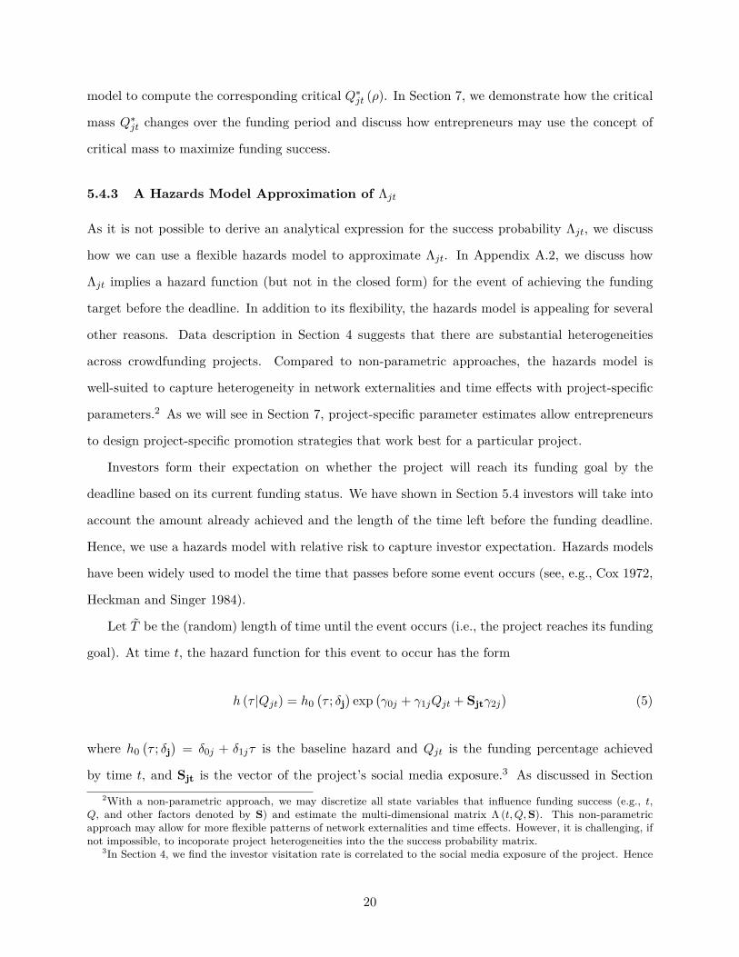
5.4.3 A Hazards Model Approximation of Λjt
As it is not possible to derive an analytical expression for the success probability Λjt, we discuss
how we can use a flexible hazards model to approximate Λjt. In Appendix A.2, we discuss how
Λjt implies a hazard function (but not in the closed form) for the event of achieving the funding
target before the deadline. In addition to its flexibility, the hazards model is appealing for several
other reasons. Data description in Section 4 suggests that there are substantial heterogeneities
across crowdfunding projects. Compared to non-parametric approaches, the hazards model is
well-suited to capture heterogeneity in network externalities and time effects with project-specific
parameters.2 As we will see in Section 7, project-specific parameter estimates allow entrepreneurs
to design project-specific promotion strategies that work best for a particular project.
Investors form their expectation on whether the project will reach its funding goal by the
deadline based on its current funding status. We have shown in Section 5.4 investors will take into
account the amount already achieved and the length of the time left before the funding deadline.
Hence, we use a hazards model with relative risk to capture investor expectation. Hazards models
have been widely used to model the time that passes before some event occurs (see, e.g., Cox 1972,
Heckman and Singer 1984).
Let T be the (random) length of time until the event occurs (i.e., the project reaches its funding
goal). At time t, the hazard function for this event to occur has the form
h (τ |Qjt) = h0(τ ; δj
)exp
(γ0j + γ1jQjt + Sjtγ2j
)(5)
where h0(τ ; δj
)= δ0j + δ1jτ is the baseline hazard and Qjt is the funding percentage achieved
by time t, and Sjt is the vector of the project’s social media exposure.3 As discussed in Section2With a non-parametric approach, we may discretize all state variables that influence funding success (e.g., t,
Q, and other factors denoted by S) and estimate the multi-dimensional matrix Λ (t, Q, S). This non-parametricapproach may allow for more flexible patterns of network externalities and time effects. However, it is challenging, ifnot impossible, to incoporate project heterogeneities into the the success probability matrix.
3In Section 4, we find the investor visitation rate is correlated to the social media exposure of the project. Hence
20

4, there is large heterogeneity in funding performance across projects. To capture unobserved
project heterogeneity, we allow parameters δj and γj in the hazard function to be project specific.
Following the hierarchical Bayes models (see, e.g., Rossi et al. 2005), we assume that project-
specific parameters, ϕj ≡ [δj, γj], are drawn from a multivariate normal distribution with mean θϕ
and variance-covariance matrix Σϕ.
At the beginning of the funding period t0 = 0, the probability that the project will reach its
goal by the deadline T j is
Λjt0 = Pr(T ≤ T j |T ≥ t0 = 0
)= 1− S
(T j |Qjt0 ,Sjt0
), (6)
where the survivor function is defined as S(t|Qjt0 ,Sjt0
)= exp
(−H
(t|Qjt0 ,Sjt0
))with the cu-
mulative hazard H (t) =∫ tt0=0 h
(τ |Qjt0 ,Sjt0
)dτ . Equation (6) links investors’ expectation on a
crowdfunding project’s success probability to the project’s current funding status Qjt0 and time
progress t0.
As time progresses and the project has not reached its goal at a given time t > t0 = 0, investors’
perceived success probability in Equation (3) becomes
Λjt(t, Qjt,Sjt, Tj , γj, δj) = Pr(T ≤ T j |T ≥ t
)=
Pr(t ≤ T ≤ T j |T ≥ 0
)Pr (T ≥ t)
=S (t|Qjt,Sjt)− S
(Tj |Qjt,Sjt
)S (t|Qjt,Sjt) = 1− exp
(−∫ T j
t
h (τ |Qjt,Sjt) dτ)
= 1− exp(− exp (γ0j + γ1jQjt + Sjtγ2j)
(δ0j
(Tj − t
)+ δ1j
2(T 2
j − t2)))
.(7)
From Equation (7), we can see that investors’ perceived success probability Λjt increases in
the accumulated funding amount Qjt if γ1j is positive (positive network externality). In addition,
this probability may be increasing, decreasing, or curvilinear in time depending on the sign and
magnitude of δ0j and δ1j . For example, if both δ0j and δ1j are positive, then investors’ perceived
success probability of the project decreases in t, i.e., the time effect is negative. The negative time
effect has an intuitive explanation: the shorter the length of time left, the less likely a project will be
able to reach its funding goal (holding other factors such as the funding amount already achieved
fixed). The hazards model in Equation (5) and the resulting success probability we derived in
we include Sjt in the hazard function.
21

Equation (7) provide a parsimonious yet flexible framework that captures both network externalities
and time effects. If the estimated γ1j , δ0j and δ1j are positive, Λjt(t, Qjt,Sjt, Tj , γj, δj) derived in
equation(7) reflects the same properties of Λjt defined in Section 5.4. Hence, Λjt(t, Qjt,Sjt, Tj , γj, δj)
can be considered as an approximation to Λjt in Section 5.4.
5.5 Backing Rate
We assume that εijt are drawn from a Type I extreme value distribution F (·) independently across
investors, projects, and time periods. The backing rate in period t follows
Ψ(t, Qjt,Sjt, Tj ,Xj, β, c, γj, δj) = 1− F(c/Λjt(t, Qjt,Sjt, Tj , γj, δj)−Xjβ
). (8)
The backing probability in Equation (8) has the same properties as investors’ perceived success
probability in Equation (8), i.e., it is increasing in Qjt if γ1j is positive , and decreasing in time if
δ0j and δ1j are positive. In addition, the backing probability is increasing in the project valuation
Xjβ. We do not restrict the signs of γ and δ in estimation. Instead, the data will inform us whether
positive network externalities and negative time effects exist.
6 Empirical Analysis and Results
We first show the goodness of fit of the proposed model over alternative specifications. Parameter
estimates of the proposed model and their implications are then discussed.
6.1 Model Comparison
We estimate the proposed (full) model and three nested models, one without network externalities,
one without time effects, and one without social media exposures. In the nested model without
network externalities, we constrain the parameter γ1j in Equation (7) to zero. As a result, investors’
backing probability at time t is not directly related to the accumulative amount of funding achieved
by that time. In the nested model without time effects, we remove the two time-effect terms, i.e.,
removing δ0j(Tj − t
)+ δ1j
2
(T 2j − t2
)in Equation (7). In this constrained model, investors’ backing
probability is not directly influenced by the length of time left. In the nested model without social
media exposures, we restrict the parameter γ1j in Equation (7) to zero.
22

Model Deviance Information Criterion (DIC)
No Network Externalities Qt 435,661
No Time Effects t 436,293
No Social Media Exposures S 434,226
Full Model 429,168
Table 5: Model Comparison Results
Model comparison results are summarized in Table 5. The deviance information criterion (DIC)
of the full model is significantly lower than that of the three nested models, suggesting that the
proposed model outperforms the nested models in goodness of model fit. Ignoring time effects lead
to the worst model fit. These model comparison results suggest that network externalities and time
effects are two essential dimensions of online crowdfunding. Incorporating both of the effects can
greatly improve the model’s predictive power.
6.2 Parameter Estimates
Estimation results from the full model are in Table 6. Parameter estimates of investors’ perceived
success probability function reveal that the network externality is positive (the estimate in row 5 is
positive) whereas the time effect is negative (the estimates in rows 6 and 7 are positive). Holding
time fixed, investors are more likely to contribute to a project that already receives a larger fraction
of funding. Holding achieved amount of funding fixed, investors are less likely to back a project
with fewer days until deadline. In the presence of a funding target and deadline, investors assess
the project’s prospect of success based on whether it can quickly attain a critical mass. The larger
the number of backers the project attains at the early stage of the funding cycle, the more likely the
project will be able to reach its funding goal by the deadline. Investors face significant opportunity
cost (see estimate of c in row 2) and may not want to contribute to a project that is not very likely
to be successfully.
Estimation of investors’ perceived success probability above may help explain the two dynamic
backing patterns observed in Figure 2. As shown in Equation (7), the positive network externality
and the negative time effect are two competing forces that determine an investor’s overall back-
ing propensity. As the funding clock ticks and the project accumulate contributions, the positive
network externality increases a investor’s backing propensity. However, as the funding cycle pro-
23

Variable Coefficients (Standard Error)
Opportunity Cost (c)
Opportunity Cost 1.1484***(0.0154) 0.9951***(0.0125)
Success Probability Function - Mean (θϕ)
Intercept -2.5664***(0.1185) -2.5913***(0.1315)
PercentFundingGoalAchieved: Qt 10.2602***(0.5818) 5.5703***(0.4540)
TimeLeft1: T − t 1.1746***(0.1674) 0.5059***(0.0817)
TimeLeft2: T 2 − t2 0.1902***(0.0310) 0.1459***(0.0251)
CumulativeFacebookActivities (log) 0.2186***(0.0324)
CumulativeTwitterActivities (log) 0.2068***(0.0643)
Success Probability Function -Variance (Σϕ)
Intercept 1.7149***(0.1779) 1.5846***(0.1588)
PercentFundingGoalAchieved: Qt 71.238***(5.6978) 16.3362***(3.3343)
TimeLeft1: T − t 2.0235***(0.3264) 0.5762***(0.0842)
TimeLeft2: T 2 − t2 0.0552***(0.0103) 0.0245***(0.0050)
CumulativeFacebookActivities (log) 0.2165***(0.0242)
CumulativeTwitterActivities (log) 0.7933***(0.0994)
Social Media (ω)
Intercept 5.9799***(0.0004) 5.9799***(0.0004)
DailyFacebookActivities (log) 0.0690***(0.0003) 0.0690***(0.0003)
DailyTwitterActivities (log) 0.0353***(0.0007) 0.0353***(0.0007)
Control of Project Characteristics (β)
FundingCycleLength (log) -0.6843***(0.0689) -0.5546***(0.0689)
Price (log) -0.7603***(0.0189) -0.5593***(0.0189)
FundingGoal (log) 0.5249***(0.0122) 0.6659***(0.0122)
CategoryDummiesAndOtherProjectCharacteristics Yes Yes
Table 6: Parameter Estimates of the Dynamic Model
24

gresses and there is less time left before the funding deadline, the investor’s expectation that the
project will reach its funding goal diminishes. The shape of a project’s observed backing pattern
(increasing, decreasing, or first decreasing and then increasing) depends on the relative strength
of these two opposing effects, which also determine the critical mass of funding the project should
attain by on time in order to achieve successful funding by the deadline. The estimation results
reveal large heterogeneity in network externalities and time effects across projects (see the estimate
of Σϕ in rows 9-12). As our model allows for project-specific network externalities and time effects,
it can capture various backing patterns observed in the dataset.
We briefly discuss the implications from the parameter estimates of project characteristics in
Table 6. Social media buzz drives more investor visits to a project. Moreover, Facebook buzz is
twice as effective as Twitter buzz (see the estimates in rows 15 and 16). entrepreneurs may promote
their projects on social media such as Facebook and Twitter to inform more potential investors.
Estimation results also indicate that setting a longer funding cycle is a double-edge sword. On one
hand, a longer funding cycle may mitigate the negative time effect we have discussed above. On the
other hand, investor valuation of a project is negatively associated with the length of the funding
cycle (see estimate of FundingCycleLength in row 17).
For expositional simplicity, we omit parameter estimates for project characteristics that are not
interesting in this paper but included are controls in the model (PhotoDemos, ProjectSocialExpo-
sure, OwnerSocialExposure, TeamSize, OwnerHasImage DescriptionLength, LinksInDescription,
ImagesInDescription, HasVideo, HasPartnership, and Category Dummies).
7 Managerial Implications and Decision Support
This section discusses how entrepreneurs can use our model to manage their crowdfunding projects.
With project-specific parameter estimates, our model may help entrepreneurs make informed deci-
sions on, for example, when to promote their project and how much promotion effort they should
do. We show that entrepreneurs of both low-valuation projects and high-valuation projects may
benefit from dynamically managing their crowdfunding campaign. The algorithm used to conduct
the managerial analyses in this section is in Appendix C.
25

7.1 Project Heterogeneity and Promotion Timing
7.1.1 Project Quality: Mean-Valuation Project vs. High-Valuation Projcet
Crowdfunding projects may fail to reach their funding target owing to low investor valuation (i.e.,
Xβ is small). As low valuation projects are difficult to excite investors, the backing probability is
low. Thus, although there are a fair number of investors who are informed about these projects,
these projects often fall far away from their funding goal by the end of the funding cycle. To
illustrate the impact of investor valuation on a project’s crowdfunding performance, we discuss
two representative projects: a mean-valuation project with Xaβ = Xβ and δa = θϕ (X is the
mean project characteristics in our dataset and θϕ is the mean of the parameter estimates), and a
high-valuation project with Xhβ and δh at the top 10% quantile among all projects. The average
number of daily visitors to a project page is around 400 in our dataset (if not considering investors
who are attracted to a project page from Facebook or Twitter activities, the mean arrival λt =
exp(ω0) ≈ 400). Other parameters are at their mean value as in Table 6. Investor arrivals follow
Mt = 400 in each period.
Figure 3(a) shows that even the mean-valuation project is almost unlikely to reach its funding
goal if the entrepreneur does not promote the project. Negative time effect dominates and investors’
backing probability decreases over time as investors believe the crowdfunding project is very likely to
be unsuccessful. The high-valuation project is much more likely to attract a critical mass of funding
(see Figure 3(b)). The negative time effect slightly dominates the positive network externality in
early periods, but the positive network externality quickly gains the upper hand in later periods.
As a result, investors’ backing probability first slightly decreases but then increases as favorable
funding outcome in early periods boots later investors’ positive belief on the prospect of the project.
As a result, funding performance takes off after the project attains the critical mass around Period
5.
7.1.2 Timing of Promotion: Early Promotion vs. Late Promotion
For a mean-valuation project, advertising on various media to attract more potential investors
is a plausible means to achieve successful funding. When designing such promotion campaigns,
entrepreneurs very often need to decide when they should execute the campaigns and at what
26

0e
+0
02
e−
04
4e
−0
46
e−
04
8e
−0
4
t
1 4 7 10 14 18 22 26 30 34 38
Ba
ckin
g R
ate
0.0
00
0.0
05
0.0
10
0.0
15
Pe
rce
nt
Go
al F
un
de
d
Backing Rate
Percent Goal Funded
(a) Mean-Valuation Project
0.0
04
0.0
06
0.0
08
0.0
10
0.0
12
0.0
14
t
1 4 7 10 14 18 22 26 30 34 38
Ba
ckin
g R
ate
0.0
0.2
0.4
0.6
0.8
1.0
Pe
rce
nt
Go
al F
un
de
d
Backing Rate
Percent Goal Funded
(b) High-Valuation Project
Figure 3: Project Valuation on Funding Success
27

Project Valuation (Quality) Early Promotion (Periods 1-10) Late Promotion (Periods 11-20)
90% Quantile Project 0 0
75% Quantile Project 300 925Mean Project (Figure 4) 2,200 8,300
25% Quantile Project 5.76× 10⁴ 3.77× 10⁵
10% Quantile Project 6.34× 10⁵ > 1.00× 10⁷
Table 7: Minimal Promotion Effort for Successful Funding: Promotion Early vs. Promotion Late
promotion level. We use our model to evaluate two promotion strategies: early promotion and
late promotion. With early promotion, the entrepreneur conducts informative advertising in early
periods (Period 1 - Period 10). With late promotion, the entrepreneur attracts additional potential
investors in later periods (Period 11 - Period 20).
Figure 4 demonstrates the crowdfunding performance of the mean-valuation project under the
two alternative promotion strategies. Early promotion is more effective. If promotion early (Periods
1-10), attracting around 2,400 each of the 10 periods is sufficient to achieve successful funding (see
Figure 4 (a)). However, if promotion later (Periods 11-20), the entrepreneur needs to attract more
than 3 times of potential investors to make the crowdfunding successful (see Figure 4(b)). This
intriguing result is due to the direct effect and indirect effect of promotion. Promotion informs a
larger number of investors and thus more contributions (direct effect). A large amount of funding
achieved in early periods also boost investors’ expectation on the prospect of the project, which
increases an individual investor’s backing propensity (indirect effect). After attaining the critical
mass of funding, the project continues to receive more contributions in later periods, even though
the entrepreneur has ceased promotion.
Table 7 summarizes the minimal promotion level required for successful funding for projects
of different “quality”. We draw these projects from the empirical distribution of project valuation
and project-specific parameters (i.e., Xjβ and δj). The result suggests that the benefit of early
promotion is considerable for a variety of projects.
28

0.0
01
0.0
02
0.0
03
0.0
04
0.0
05
0.0
06
1 4 7 10 14 18 22 26 30 34 38
Ba
ckin
g R
ate
0.0
0.2
0.4
0.6
0.8
1.0
1.2
1.4
Pe
rce
nt
Go
al F
un
de
d
t
Percent Goal Funded
(Promtn E!ort=1.2K)
Percent Goal Funded
(Promtn E!ort=2.4K)
Backing Rate
(Promtn E!ort=2.4K) Backing Rate
(Promtn E!ort=1.2K)
(a) Early Promotion (Periods 1-10)
0.0
00
0.0
01
0.0
02
0.0
03
0.0
04
0.0
05
0.0
06
t
1 4 7 10 14 18 22 26 30 34 38
Ba
ckin
g R
ate
0.0
0.2
0.4
0.6
0.8
1.0
1.2
Pe
rce
nt
Go
al F
un
de
d
Backing Rate (Promtn E!ort=6K)
Percent Goal Funded
(Promtn E!ort=6K)
Percent Goal Funded
(Promtn E!ort=8.4K)
Backing Rate (Promtn E!ort=8.4K)
(b) Late Promotion (Periods 11-20)
Figure 4: Impact of Promotion on Funding Performance of the Mean-Valuation Project
29

7.2 Funding Uncertainty and Dynamic Promotion
7.2.1 Uncertain Investor Arrivals
Online crowdfunding is subject to various risks and uncertainty (Agrawal et al. 2013). Descriptive
statistics in Table 2 show that there are large fluctuations in daily investor visits to a project. In
our dataset, even high-valuation projects may fail to attain a critical mass of funding if the project
fails to inform a relatively number of potential investors at the early stage of the funding cycle
(e.g., investor visits Mt is too small in early periods).
To reveal the impact of stochastic investor arrivals during the funding cycle, we simulate 1,000
realizations of investor visitation processes {Mt}Tt=1, whereMt follows a stationary distribution with
mean 400 (same level as in the deterministic case in Section 7.1). Details of the simulation algorithm
are in Appendix C. Without uncertainty (i.e., standard deviation is zero), the high-valuation project
is sure to reach its funding goal, as demonstrated in Figure 3(b). With uncertainty, the project is
only able to hit this target in 660 out of 1,000 scenarios (i.e., success rate is 66%).
Figure 5 shows two realizations from the simulations. In Periods 1-6, investor arrivals and
funding performance are similar in both scenarios. However, in Scenario II, unfavorable shocks
occur in Periods 7-15 (see the dashed red curve in Figure 5(a)). There are a small number of
visitors and thus a small number of contributions. Although exogenous shocks are stationary,
the accumulative funded amount Qjt is path-dependent. A small number of investor arrivals in
Periods 7-15 not only result in small contributions in these periods, but also negatively influence
later investors’ expectations on the project’s success probability. Therefore, even though there are
relatively large numbers of investor arrivals in later periods, the backing probability is low and thus
the total number of contributions does not recover from the previous negative shocks (see the solid
red curve in Figure 5(b)). In Scenario I, however, there are no big negative shocks in early periods
so the project is able to reach a critical mass around Period 8 (see the solid black curve in Figure
5(b)). After reaching this critical point, funding performance takes off, despite the unfavorable
shocks in later periods. These results show that entrepreneurs should actively monitor and plan
interventions for their crowdfunding projects.
30

02
00
40
06
00
80
0
Co
nsu
me
r A
rriv
als
1 4 7 10 14 18 22 26 30 34 38
t
Scenario I
Scenario II
(a) Investor Arrivals
0.0
00
0.0
05
0.0
10
0.0
15
0.0
20
1 4 7 10 14 18 22 26 30 34 38
Ba
ckin
g R
ate
0.0
0.2
0.4
0.6
0.8
1.0
1.2
1.4
Pe
rce
nt
Go
al F
un
de
dBacking Rate - I
Percent Goal Funded - I
Percent Goal Funded - II
Backing Rate - II
t
(b) Funding Performance
Figure 5: The impact of exogenous random shocks on funding performance of the high-valuationproject. Investor arrivals to the project follow a stationary distribution with mean 400.
31

7.2.2 Time-Varying Critical Mass and Dynamic Promotion
The analysis above reveals that crowdfunding projects may fail due to low project valuation and/or
unfavorable shocks. Facing negative shocks, entrepreneurs may advertise their project to increase
the chance of successful funding. However, such promotion efforts are not costless. To increase
the return on marketing investment, entrepreneurs should know when to execute their promotion
campaigns. To help entrepreneurs maximize return on marketing investment using our model, we
design a dynamic promotion strategy which provides entrepreneurs a road map to determine when
it is necessary for they to intervene in the funding process.
Observing the current funding status (t, Qt), entrepreneurs may use the simulation procedure we
develop in Appendix C to evaluate the success probability of the project. If the success probability
is lower than the targeted level, entrepreneurs may advertise their project to inform more potential
investors. In the heat maps in Figure 6, we compute the minimal promotion level required in order
to achieve a success rate of 0.9 for each (t, Qt) combination. The white color corresponds to the
cases where no additional advertising is needed, whereas the darker the red color, the higher the
promotion level is required.
The presence of positive network externalities and negative time effects jointly leads to a critical
mass for funding success, and this critical mass changes over time. If the funding performance
falls below the critical mass, entrepreneurs should promote their project to attract more potential
investors. For example, the mean-valuation entrepreneur needs to seed at Level 17 (attracting
additional 850 visitors) if the project has achieved less than 8% of its funding goal by Period 10
(see Figure 6(a)). However, the high-valuation entrepreneur only needs to seed the project at Level
2 (attracting additional 100 visitors), as shown in Figure 6(b). These heat maps offer important
decision support for entrepreneurs to dynamically manage their crowdfunding projects.
8 Model Robustness Checks
In this section, we conduct several robustness checks to explore the validity of our model of investors’
perceived project success probability.
Project Fixed Effects Although we have included rich controls of project characteristics, there
might be unobserved heterogeneity not captured by the project valuation function in Equation (4).
32

0.00
0.25
0.50
0.75
1.00
0 10 20 30 40
t
Q
0
5
10
15
20
25
Promtn E�ortTim
e-Vary
ing C
ritical M
ass
(a) Mean-Valuation Project
0.00
0.25
0.50
0.75
1.00
0 10 20 30 40
t
Q
0
5
10
15
20
25
Promtn E�ort
Tim
e-V
aryi
ng
Cri
tica
l Mas
s
(b) High-Valuation Project
Figure 6: Given the current project status (t, Qt), the minimal promotion effort (from period t+ 1on) required to achieve a success rate of 0.9. A promotion level of 1 corresponds to attractingadditional 50 visitors.
33

Variable Project Fixed Effects Excluding First 3 Days Alternative Qjt
Success Probability - Mean (θϕ)
PercentFundingGoalAchieved: Qt 4.7161***(0.2239) 4.5049***(0.2843) 4.7143***(0.2849)
TimeLeft1: T − t 0.4053***(0.0442) 0.3753***(0.1437) 0.3553***(0.1232)
TimeLeft2: T 2 − t2 0.1259***(0.0089) 0.1763***(0.0270) 0.1663***(0.0282)
CumulativeFacebookActivities (log) 0.3801***(0.0445) 0.2611***(0.0348) 0.2511***(0.0333)
CumulativeTwitterActivities (log) 0.1538* (0.0979) 0.2084***(0.0651) 0.1998***(0.0648)
Success Probability -Variance (Σϕ)
PercentFundingGoalAchieved: Qt 12.2903***(1.4629) 16.3362***(3.3343) 16.8562***(3.4335)
TimeLeft1: T − t 0.4006***(0.0355) 0.5762***(0.0845) 0.5526***(0.0842)
TimeLeft2: T 2 − t2 0.0248***(0.0050) 0.0245***(0.0052) 0.0241***(0.0050)
CumulativeFacebookActivities (log) 0.3131** (0.1520) 0.2165***(0.0242) 0.2065***(0.0237)
CumulativeTwitterActivities (log) 1.1921***(0.3448) 0.7933***(0.0994) 0.7633***(0.0973)
Table 8: Parameter Estimates of the Success Belief Function under Alternative Specifications
To address this, we include project fixed effects and extend the investors’ project valuation function
as follow:
υijt = Xjβ + ξj + εijt.
Parameter estimates in the second column of Table 8 show that our main model is robustness to
unobserved project heterogeneity.
Friends/Family in Early Stage of Funding It is likely that a entrepreneur’s friends and family
might play a role in early stage of the funding cycle (Agrawal et al. 2013). Unfortunately, we do
not know which backers are friends/family, neither does the owner of crowdfunding platform. Even
if we knew which backers were friends/family, it is not clear what their utility function looks like.
To alleviate the concern of friends/family in our model estimation, we exclude observations of early
backers (all observations in the first 3 days of the funding cycle). The remainder of the observations
under this sample would then be more likely to capture the behavior of self-interested backers.
Model estimates, as shown in the third column of Table 8, remain similar to those in our
main model. This suggests that friends/family might only account for an insignificant fraction
of backers, or they do not behave quite differently from other backers. Similar to Agrawal et al.
2013, we observe in our dataset that a large number of projects raise almost nothing from anyone,
including friends and family. This might suggest that backers (including friends/family) may not
34

want to support projects that are unlikely to be successful.
Alternative Measure of Current Funding Status Qjt With our aggregate daily data, we do not
observe the exact timing of each investor visit/contribution within a day. We have measured the
current funding status Qjt as the percent of funding goal achieved by the end of period t − 1,
which does not allow variation within a given day. This Qjt is likely to be lower than the true
funding performance seen by potential investors when they visit the project page (especially for
late arrivals). As a robustness check, we use an alternative measure of current funding performance:
the average of the percentage of funding goal achieved on day t − 1 and day t. In contrast to the
current measure Qjt, this alternative measure Q′jt is more accurate for late coming visitors on a
given day, but less accurate for early coming visitors. The current measure and alternative measure
would give the upper and lower bound for the true effect of network externalities. We re-estimate
the model and find that the parameter estimates remain very similar. This result is expected as
the funding cycle is relatively long (with the mean of 40 days as shown in the descriptive statistics
in Table 2) and the number of new backers per day is not very large (with the mean of 1.31).
9 Conclusion
This research builds a dynamic model to study how investors decide whether to contribute to a
project based on current funding performance and time progress. We model the time effect using
a hazards model that captures the success probability of a crowdfunding project. The proposed
model extends the traditional static view of network externalities by incorporating the timing of
achieving a certain network size. Model estimation shows that investors are more likely to contribute
to a project that has already received a sufficiently large number of backers in a timely manner.
Investors are less likely to back a project with little time left to achieve its funding target. Investors
face a relative large opportunity cost and may not want to contribute to a project that is not very
likely to be successfully funded. These two competing forces (positive network externalities and
negative time effects) determine an investor’s overall backing propensity. If the negative time effect
dominates the positive network externality, investors become less likely to contribute to a project
in later periods. However, if the positive network externality dominates, investors are more likely
to contribute in later periods. These two competing forces give rise to a critical mass of funding the
35

project should attain on time in order to achieve successful funding by the deadline. Our results
shed light on the complex dynamic mechanism and uncertainty in the crowdfunding process which
has yet to be unraveled to researchers and practitioners so far.
This research contributes to the emerging literature on online crowdfunding. None of the
existing studies have formulated the dynamic crowdfunding process and looked into the interaction
between network externalities and a finite funding cycle. The proposed model provides an economic
framework to understand investors’ dynamic decision behaviors and the resulting funding patterns.
Our research provides important implications for entrepreneurs and crowdfunding platforms. We
demonstrate that crowdfunding projects may fail to reach their funding target due to low investor
valuation. High-valuation projects may also fail to attain a critical mass of funding because of
unfavorable shocks at the early stage of the funding cycle. Our research provides actionable guidance
on how to design a crowdfunding campaign and helps entrepreneurs decide when and how much
they should promote their project on social media to maximize the return on marketing investment.
This research is not without limitations. As our objective is to provide a parsimonious framework
for modeling network externalities and time effects, future research can construct a more complex
model for strategic interactions between investors. On the crowdfunding platform we study in
this paper, backers are individual, inexperienced consumers rather than professional, institutional
investors. Therefore, our results might not directly apply to other empirical settings such as equity-
based crowdfunding. However, if there is empirical evidence that some sophisticated institutional
investors may optimally time their backing decisions and make their own decisions to influence
others, it is possible to extend our model to incorporate these behaviors. Satisfactory identification
of such strategic behaviors will require individual-level investor data on investor characteristics, visit
history, and backing time, which are beyond the scope of the current dataset (our daily aggregate
dataset does not allow us to track an individual investor’s dynamic behaviors such as multiple visits
to a project). Future research may also look into the behaviors of entrepreneurs in the funding
cycle. A flexible model that allows suboptimal strategies will help capture the bounded rationality
of entrepreneurs in this empirical setting.
36

References
Agrawal, A.K, C. Catalini, A. Goldfarb. 2013. Some simple economics of crowdfunding. Working Paper,
National Bureau of Economic Research (2013).
Anand, K.S., R. Aron. 2003. Group buying on the web: A comparison of price-discovery mechanisms.
Management Science 49(11) 1546–1562.
Bijwaard, G.E., P.H. Franses, R. Paap. 2006. Modeling purchases as repeated events. Journal of Business
& Economic Statistics 24(4) 487–502.
Brynjolfsson, E., C.F. Kemerer. 1996. Network externalities in microcomputer software: An econometric
analysis of the spreadsheet market. Management Science 42(12) 1627–1647.
Burtch, G., A. Ghose, S. Wattal. 2013. An empirical examination of the antecedents and consequences of
contribution patterns in crowd-funded markets. Information Systems Research 24(3) 499–519.
Cox, D.R. 1972. Regression models and life tables (with discussion). Journal of the Royal Statistical Society
34 187–220.
Dubé, J.-P., G.J. Hitsch, P.K. Chintagunta. 2010. Tipping and concentration in markets with indirect
network effects. Marketing Science 29(2) 216–249.
Economist. 2010. Putting your money where your mouse is. Economist (September 2, 2010) Available at
http://www.economist.com/node/16909869.
Heckman, J.J., B. Singer. 1984. A method for minimizing the impact of distributional assumptions in
econometric models for duration data. Econometrica 52(2) 271–320.
Hu, M., M. Shi, J. Wu. 2013. Simultaneous versus sequential group-buying mechanisms. Management
Science 59(12) 2805–2822.
Jing, X., J. Xie. 2011. Group buying: a new mechanism for selling through social interactions. Management
Science 57(8) 1354–1372.
Katz, M.L, C. Shapiro. 1986. Technology adoption in the presence of network externalities. Journal of
Political Economy 94(4) 822–841.
Katz, M.L., C. Shapiro. 1992. Product introduction with network externalities. Journal of Industrial Eco-
nomics 40(1) 55–83.
Kauffman, R.J, J. McAndrews, Y.M. Wang. 2000. Opening the “black box” of network externalities in
network adoption. Information Systems Research 11(1) 61–82.
Kauffman, R.J, B. Wang. 2002. Bid together, buy together: On the efficacy of group-buying business models
in internet-based selling. The E-Business Handbook (CRC Press Boca, Raton, FL).
37

Kim, J.H., P.W. Newberry, C. Qiu. 2015. An empirical analysis of a crowdfunding platform. NET Institute
Working Paper .
Kuppuswamy, V., B.L. Bayus. 2013. Crowdfunding creative ideas: The dynamics of project backers in
kickstarter. Working Paper, University of North Carolina at Chapel Hill (2013).
Lenk, P.J., A.G. Rao. 1995. Transition times: Distributions arising from time heterogeneous poisson pro-
cesses. Management Science 41(7) 1117–1129.
Lowry, P.B., J. DÁrcy, B. Hammer, G.D. Moody. 2016. cargo cultscience in traditional organization and
information systems survey research: A case for using nontraditional methods of data collection, in-
cluding mechanical turk and online panels. Journal of Strategic Information Systems 25(3) 232–240.
Marwell, N.B. 2015. Competing fundraising models in crowdfunding markets. Working Paper, University of
Wisconsin-Madison .
Mollick, E. 2014. The dynamics of crowdfunding: An exploratory study. Journal of Business Venturing
29(1) 1–16.
Paolacci, G., J. Chandler, P.G. Ipeirotis. 2010. Running experiments on amazon mechanical turk. Judgment
and Decision making 5(5) 411–419.
Rossi, P.E., G.M. Allenby, R.E. McCulloch. 2005. Bayesian Statistics and Marketing. Wiley, New York.
Schwienbacher, A., B. Larralde. 2012. Crowdfunding of small entrepreneurial ventures. Handbook of En-
trepreneurial Finance (Oxford University Press, Cary, NC).
Stokey, N.L., R.E. Lucas, E.C. Prescott. 1989. Recursive Methods in Economic Dynamics. Harvard University
Press.
Susarla, A., J.H. Oh, Y. Tan. 2012. Social networks and the diffusion of user-generated content: Evidence
from youtube. Information Systems Research 23(1) 23–41.
Zhang, J., P. Liu. 2012. Rational herding in microloan markets. Management science 58(5) 892–912.
Zhang, K., T. Evgeniou, V. Padmanabhan, E. Richard. 2012. Content contributor management and network
effects in a UGC environment. Marketing Science 31(3) 433–447.
38

Appendix
A Analysis of the Funding Success Probability
In this appendix, we first prove the analytical properties of the funding success probability Λt.
Following the recursive definite of Λt, we can prove Proposition 1 by mathematical induction. We
then discuss how the funding success probability in Equation (7) is implied by the expected funding
success probability of the investors. For expositional simplicity, we drop the project index j.
A.1 Recursive Definition of Λt and the Proof of Its Properties
We can divide the entire funding period into a large number of intervals, t = 1, . . . , T , such that
the number of the random arrival of potential investors in period t, Mjt can either be one or zero.
This is a property of the Poisson process model for investor visitation in Section 5.2. When the
time interval t is small enough, the probability of having more than one investors arriving in t
approaches zero. In reality, if we divide the entire funding cycle into many small time periods, we
will only observe at most one arrival of a potential investor in a period (Marwell 2015).
We use a recursive approach and derive Λjt by backward induction (Stokey et al. 1989). Suppose
there are a finite number of periods t = 1, . . . , T . The project is successfully funded if the total
number of backers in the total T periods exceed a target number NjG (or equivalently, the total
amount of funding pledged exceed the funding goal Gj = NjG · Pj). Let gjt the additional number
of backers needed to reach the goal NjG.
In the last period T , we can derive ΛjT as follows:
1) if gjT ≤ 0, then the project is already successfully funded, i.e., ΛjT = 1;
2) if gjT > 1, then the project is unlikely to be successfully funded, i.e., ΛjT = 0;
3) if gjT = 1, then the project will be successfully funded if a consumer arrives AND decides to
invest. This happens with probability
ΦjT = Pr(MjT = 1
)Pr(εijT ≥ c− vj
),
where Pr(MjT = 1
)the probability that an investor arrives in period T and Pr
(εijT ≥ c− vj
)the
probability that the investor invests in the project.
39

In summary, we have in period T ,
ΛjT(gjT
)=
1, if gjT ≤ 0,
ΦjT
(gjT
), if 1 ≤ gjT < 0,
0, if gjT > 1.
In period T − 1, we can derive Λj(T−1)
(gj(T−1)
)given ΛjT
(gjT
)as follows:
1) if gj(T−1) ≤ 0, then the project is already successfully funded, i.e., Λj(T−1) = 1;
2) if gj(T−1) > 2, then the project is unlikely to be successfully funded, i.e., Λj(T−1) = 0;3) if 2 ≥ gj(T−1) > 0, then the funding success probability is
Φj(T−1)(gj(T−1)
)=
[Pr(Mj(T−1) = 0
)+ Pr
(Mj(T−1) = 1
)Pr(εij(T−1) < c/ΛjT
(gj(T−1) − 1
)− vj
)]ΛjT
(gj(T−1)
)+ Pr
(Mj(T−1) = 1
)Pr(εij(T−1) ≥ c/ΛjT
(gj(T−1) − 1
)− vj
)ΛjT
(gj(T−1) − 1
),
where Pr(Mj(T−1) = 0
)is the probability that an investor does not arrives,
Pr(Mj(T−1) = 1
)Pr(εij(T−1) < c/ΛjT
(gj(T−1) − 1
)− vj
)is the probability that an investor arrives but chooses not to invest, and
Pr(Mj(T−1) = 1
)Pr(εij(T−1) ≥ c/ΛjT
(gj(T−1) − 1
)− vj
)is the probability that an investor arrives and invests, which reduces the remaining funding target
by 1 to gj(T−1) − 1.
In summary, we have in period T − 1,
Λj(T−1)
(gj(T−1)
)=
1, if gj(T−1) ≤ 0,
Φj(T−1)
(gj(T−1)
), if 2 ≥ gj(T−1) > 0,
0, if gj(T−1) > 2.
(9)
Therefore, for any general period 1 ≤ t− 1 ≤ T , given Λjt (gjt) of the following period, we have
40

Λj(t−1)(gj(t−1)
)=
1, if gj(t−1) ≤ 0,
Φj(t−1), if T − t+ 1 ≤ gj(t−1) < 0,
0, if gj(t−1) > T − t+ 1,
(10)
where
Φj(t−1)(gj(t−1)
)=
[Pr(Mj(t−1) = 0
)+ Pr
(Mj(t−1) = 1
)Pr(εij(t−1) < c/Λjt
(gj(t−1) − 1
)− vj
)]Λjt(gj(t−1)
)+ Pr
(Mj(t−1) = 1
)Pr(εij(t−1) ≥ c/Λjt
(gj(t−1) − 1
)− vj
)Λjt(gj(t−1) − 1
).
Proof of Proposition 1
Proof.
(i) We first show that Λt is decreasing in g by induction.
For t = T , it is obvious that ΛT (g)− ΛT (g − 1) ≤ 0, i.e., ΛT is (weakly) decreasing in g.Suppose Λt+1 (g) is decreasing in g. We would like to show that Λt (g) is also decreasing in g.
This is obvious if g ≤ 0 and g ≥ T − t. Thus, we only need to show that Λt (g) is also decreasingin g for 0 < g < T − t . Note that
Λt (g) = Pr (Mt = 0) Λt+1 (g) (11)
+ Pr (Mt = 1) Pr(
εit <c
Λt+1 (g − 1) − v
)Λt+1 (g) + Pr (Mt = 1) P r
(εit ≥ c
Λt+1 (g − 1) − v
)Λt+1 (g − 1)
≤ Pr (Mt = 0) Λt+1 (g)
+ Pr (Mt = 1) Pr(
εit <c
Λt+1 (g − 1) − v
)Λt+1 (g − 1) + Pr (Mt = 1) Pr
(εit ≥ c
Λt+1 (g − 1) − v
)Λt+1 (g − 1)
= Pr (Mt = 0) Λt+1 (g) + Pr (Mt = 1) Λt+1 (g − 1)
and
Λt (g − 1) = Pr (Mt = 0) Λt+1 (g − 1) (12)
+ Pr (Mt = 1) Pr(
εit <c
Λt+1 (g − 2) − v
)Λt+1 (g − 1) + Pr (Mt = 1) Pr
(εit ≥ c
Λt+1 (g − 2) − v
)Λt+1 (g − 2)
≥ Pr (Mt = 0) Λt+1 (g − 1)
+ Pr (Mt = 1) Pr(
εit <c
Λt+1 (g − 2) − v
)Λt+1 (g − 1) + Pr (Mt = 1) Pr
(εit ≥ c
Λt+1 (g − 2) − v
)Λt+1 (g − 1)
= Pr (Mt = 0) Λt+1 (g − 1) + Pr (Mt = 1) Λt+1 (g − 1)
≥ Pr (Mt = 0) Λt+1 (g) + Pr (Mt = 1) Λt+1 (g − 1) .
Therefore, we have Λt (g) ≤ Λt (g − 1), i.e., Λt (g) is decreasing in g.
41

(ii) We now show that Λt is decreasing in t. This is obvious if g ≤ 0 and g ≥ T − t. Thus, weonly need to show that Λt (g) is also decreasing in t for 0 < g < T − t . From Equation (10), wehave for any 1 ≤ t ≤ T − 1,
Λt (g) = Pr (Mt = 0) Λt+1 (g) (13)
+ Pr (Mt = 1) Pr(
εit <c
Λt+1 (g − 1) − v
)Λt+1 (g) + Pr (Mt = 1) Pr
(εit ≥ c
Λt+1 (g − 1) − v
)Λt+1 (g − 1)
≥ Pr (Mt = 0) Λt+1 (g)
+ Pr (Mt = 1) Pr(
εit <c
Λt+1 (g − 1) − v
)Λt+1 (g) + Pr (Mt = 1) Pr
(εit ≥ c
Λt+1 (g − 1) − v
)Λt+1 (g)
= Pr (Mt = 0) Λt+1 (g) + Pr (Mt = 1) Λt+1 (g)
= Λt+1 (g) .
The inequality holds because Λt+1 (g − 1) ≥ Λt+1 (g) as shown in part (i). Therefore, we have
Λt (g) ≥ Λt+1 (g), i.e., Λt is decreasing in t .
A.2 A Hazards Model Approximation
In this section, we show how Λt implies a hazard function which inherits the properties of Λt.
Though the proportional hazards model in Section 5.4.3 is not the analytical solution from Λt from
Equation (10), it is a good approximation that captures the properties of the problem.
For mathematical clarity, we write Λt (gt) as Λ (t, gt) and treat t as a continuous variable (when
the number of periods approaches infinity and the time interval in each period becomes infinitesi-
mally small, we may treat t as a continuous variable). Λ (t, gt) will have the same properties of Λt
because the proof in Appendix 1 is true for any number of T periods. Let T be the random time
when the project is 100% successfully funded, i.e., when gT = 0. In this fashion, Λ (t, gt) can be
written as
Λ (t, gt) = Pr(t < T ≤ T |T ≥ t, gt
)=
Pr(t < T ≤ T |gt
)Pr (T > t|gt)
=Pr (T > t|gt)− Pr
(T > T |gt
)Pr (T > t|gt)
= 1−Pr(T > T |gt
)Pr (T > t|gt)
.
Therefore, we have
Pr (T > t|gt) =Pr(T > T |gt
)1− Λ (t, gt)
.
42

If we treat Pr (T > t|gt) as a survivor function, we can let
h (t, gt) = −∂ Pr (T > t|gt) /∂tPr(T > t|gt
) = −∂ log (Pr (T > t|gt))∂t
= ∂ log (1− Λ (t, gt))∂t
.
Because we have shown that Λ (t, gt) is decreasing in t, it is straightforward to show that h (t, gt) ≥ 0,
which can be construed as a hazard function. However, we do not have a closed-form solution for
Λ (t, gt). As a result, we approximate h (t, gt) using a proportional hazard function
h (t, gt) = h0 (t; δ) exp (γ0 + γ1gt) ,
which will lead to the same properties of Λ (t, gt) if γ1 > 0.
B Estimation Procedure
B.1 Summary of the Bayesian Hierarchical Model
We develop a dynamic model of consumer choices with network externalities and time effects. Given
the hierarchical nature of the model, we cast it in the Bayesian hierarchical framework. The full
specification of the model is
Njt|t, Qjt,Sjt, Tj ,Xj, β, c, γj, δj,
Mjt|sjt, , ω,
43

with the following parameters to be estimated
β ∼MVNKβ (θβ, Σβ) ,
c ∼ Gamma(ac, bc
),
ω ∼MVNKω (θω, Σω) ,
ϕj = [γj, δj] ∼MVNKϕ (θϕ, Σϕ) ,
θϕ ∼MVNKϕ
(θϕ, Σϕ
),
Σϕ ∼ IWϕ
(S−1, ν
),
where Kβ is the dimension of the vector of project characteristics, Kϕ is the dimension of the
vector of project-specific parameters in the hazards model, and Kω is the dimension of the vector
of social media activities. As illustrated Section 5.1, each of the parameters plays a distinct role
in the data-generating process, so the parameters to be estimated should be identified. Estimation
with a simulated dataset confirms that the model is identified (results available upon request).
B.2 Likelihood-Based Estimation
We observe the number of investor visits and contributions in each period. Let Mjt denote the
number of visitors to project j in period t, then, Njt, the number of backers who decide to contribute
to the project in that period is
Njt = MjtΨ(t, Qjt,Sjt, Tj ,Xj, β, c, γj, δj). (14)
The likelihood for observations dataj ≡ {Qjt, Tj ,Xj,Sjt} from project j over the T j periods is
Lj(dataj |β, c, ω, γj, δj
)=
T j∏t=1
{Ψ(t, Qjt,Sjt, Tj ,Xj, β, c, γj, δj)Njt
×(1−Ψ(t, Qjt,Sjt, Tj ,Xj, β, c, γj, δj)
)Mjt−Njt
× Pois(Mjt|ω,Sjt
)}.
44

Pooling the data from the J projects, the likelihood for all observations is
L (data|β, c, ω, γ, δ) =∏Jj=1 Lj
(dataj |β, c, ω, γj, δj
).
Identification of the parameters comes from the rich variations in the panel dataset. The
variations in investor arrival rates across projects help identify ω, the overall funding performance
across projects help identify β, and the variations of time-varying funding patterns across projects
helps identify δ, γ, and c. We estimate the model using Bayesian inference with the Markov Chain
Monte Carlo (MCMC) method as follows.
Step 1. Sample β
We assume the prior distribution of β followsMVNKβ (θβ, Σβ), where θβ = 0 and Σβ = 104IKβ
(IKβ is an Kβ × Kβ identity matrix). We use Metropolis-Hastings sampling with random-walk
to generate the next draw β∗ from a normal distribution, i.e., β∗k ∼ N(βk, σ
2k
). The accepting
probability for β∗ is
min{L (β∗, c, ω, ϕ|Data)MVNKβ (β∗|θβ, Σβ)L (β, c, ω, ϕ|Data)MVNKβ (β|θβ, Σβ) , 1
}
Step 2. Sample c
We consider the prior distribution of c following Gamma(ac, bc
), where ac = 1
2 and bc = 12 . We
use Metropolis-Hastings sampling with random-walk to generate the next draw c∗ from a log-normal
distribution, i.e., c∗ ∼ log−N(log (c) , σ2
c
). Hence, the accepting probability for c∗ is
min
L (β, c∗, ω, ϕ|Data)Gamma(c∗|ac, bc
)c∗
L (β, c, ω, ϕ|Data)Gamma(c|ac, bc
)c, 1
where the last terms in the numerator and denominator correspond to the Jacobian in the log-
normal proposal function.
Step 3. Sample ω
We assume the prior distribution of ω followsMVNKω (θω, Σω), where θω = 0 and Σω = 104IKω
(IKω is an Kω × Kω identity matrix). We use Metropolis-Hastings sampling with random-walk
to generate the next draw ω∗ from a normal distribution, i.e., ω∗k ∼ N(βk, σ
2k
). The accepting
45

probability for ω∗ is
min{L (β, c, ω∗, ϕ|Data)MVNKω (ω∗|θω, Σω)L (β, c, ω, ϕ|Data)MVNKω (ω|θω, Σω) , 1
}
Step 4. Sample ϕj ≡ [δj, γj]
We consider the prior distribution of ϕj followingMVNKϕ (θϕ, Σϕ). We use Metropolis-Hastings
sampling with random-walk to generate the next draw ω∗ from a normal distribution, i.e., ϕ∗jk ∼
N(ϕjk, σ
2k
). The accepting probability for ϕ∗j is
min
L(β, c, ω, ϕ∗j |Data
)MVNKϕ
(ϕ∗j |θϕ, Σϕ
)L(β, c, ω, ϕj|Data
)MVNKϕ
(ϕj|θϕ, Σϕ
) , 1
As there are not enough observations for projects with only one backer, we pool these projects
such that they share the same project-specific parameters ϕj.
Step 5. Sample θϕ
We consider the conjugate prior distribution for θϕ following MVNKϕ
(θϕ, Σϕ
), where θϕ = 0
and Σϕ = 104IKϕ . The next draw θ∗ϕ is drawn from a multivariate normal distribution
θ∗ϕ ∼MVNKϕ (A,B) ,
where
A = B′
J∑j=1
ϕj
′Σ−1ϕ + θ′ϕΣ
−1ϕ
′ ,B =
(IΣ−1
ϕ + Σ−1ϕ
)−1.
Step 6. Sample Σϕ
We consider the conjugate prior distribution for Σϕ following an inverse Wishart distribution
IWKϕ
(S−1, ν
), where S = IKϕ and ν = 1. The next draw Σ∗ϕ is drawn from an inverse Wishart
distribution
Σ∗ϕ ∼ IWKϕ
J∑j=1
(ϕj − θϕ
) (ϕj − θϕ
)′ + S
−1
, I + ν
.
46

C Simulation Algorithm
We first present a general algorithm used to simulate investor behaviors and backing decisions,
followed by additional details on how we conduct each of the managerial analyses in Section 7. For
simplicity of exposition, we drop the project index j.
The investor valuation of the project is υit = v + εit, where εit follow a Type I extreme value
distribution. The algorithm uses the analytical expression in Equation (8) to compute investors’
backing probability. The mean investor arrival λt = exp (ω0 + ηt), where ηt are visitation shocks
drawn from a normal distribution N(0, σ2). Parameters {c, ω0, γ, δ} are at their estimated mean
value in Table 6. Alternatively, we can draw parameter value from their posterior distribution,
which is computationally more demanding. Suppose the current funding status is (t, Qt), the
general algorithm simulate the impact of promotion at amount s from periods t+ 1 to T (i.e., the
end the funding cycle).
Simulation Algorithm
1. Simulate R (R = 1, 000) realizations of investor visits {Mt′}Tt′=t+1 for the remainder of T ′
periods (T ′ = T − t ), where Mt′ ∼ Pois(λt). The mean arrival λt = exp (ω0 + ηt), where ηt is
drawn from a normal distribution N(0, σ2).
2. For each realization of investor visits r := 1 : R
2.1 For each period t′ := (t+ 1) : T
2.1.1 Compute the backing probability
Ψrt′ = 1
1 + exp(
cΛt(t′,Qrt′−1,T ,γ,δ)
−Xβ) .
2.1.2 If promotion level of st′ is conducted in period t′, then
M rt′ = M r
t′ + st′ .
2.1.3 Compute the number of backers in period t′
N rt′ = M r
t′Ψrt′ .
47

2.1.4. Update the fraction of funding achieved up to time t′
Qrt′ = Qrt′−1 + N rt′P
G.
3. Compute the success rate of the crowdfunding project as the fraction of the R scenarios where
the final achieved funding amount is greater than 1, i.e.,
SuccessRate =#{Qr
T≥ 1, r = 1, 2, ..., R}
R.
We now provide additional details on how we adapt the general algorithm above to do each of
the managerial analyses in Section 7. In investigation of the impact of project valuation (Figure
3), the starting funding status is the initiate stage of the project, i.e., (t = 0, Q0 = 0). There are
no exogenous shocks (σ = 0) and no promotion (st′ = 0) for t′ = 1, 2, .., T . In evaluation of the
impact of promotion, the promotion level is as described in the caption of Figure 4.
In evaluation of the impact of exogenous shocks (Figure 5), the starting funding status is set as
the initiate stage of a project, i.e., (t = 0, Q0 = 0). Standard deviation of the shocks computed from
the investor visitation data is σ = 1. There is no promotion (st′ = 0) for t′ = 1, 2, .., T . In creating
the heat maps in Figure 6, we repeat the simulation for each combination of (t, Q), t = 1, 2, .., T
and Q = 0, 0.025, .., 1. For each combination, we search for the minimal promotion level needed
to achieve the targeted success rate (e.g., 0.9). This is done by starting at promotion level 0 (i.e.,
st′ = 0) and increasing this level until the success rate exceeds the targeted one.
48