Embed Size (px)
Citation preview

Network Capacity Assessment of CHP-based Distributed Generation
on Urban Energy Distribution Networks
by
Xianjun Zhang
A Dissertation Presented in Partial Fulfillment
of the Requirements for the Degree
Doctor of Philosophy
Approved March 2013 by the
Graduate Supervisory Committee:
George Karady, Chair
Samuel Ariaratnam
Keith Holbert
Jennie Si
ARIZONA STATE UNIVERSITY
May 2013

i
ABSTRACT
The combined heat and power (CHP)-based distributed generation (DG) or dis-
tributed energy resources (DERs) are mature options available in the present energy mar-
ket, considered to be an effective solution to promote energy efficiency. In the urban en-
vironment, the electricity, water and natural gas distribution networks are becoming in-
creasingly interconnected with the growing penetration of the CHP-based DG. Subse-
quently, this emerging interdependence leads to new topics meriting serious considera-
tion: how much of the CHP-based DG can be accommodated and where to locate these
DERs, and given preexisting constraints, how to quantify the mutual impacts on opera-
tion performances between these urban energy distribution networks and the CHP-based
DG.
The early research work was conducted to investigate the feasibility and design
methods for one residential microgrid system based on existing electricity, water and gas
infrastructures of a residential community, mainly focusing on the economic planning.
However, this proposed design method cannot determine the optimal DG sizing and sit-
ing for a larger test bed with the given information of energy infrastructures. In this con-
text, a more systematic as well as generalized approach should be developed to solve
these problems.
In the later study, the model architecture that integrates urban electricity, water
and gas distribution networks, and the CHP-based DG system was developed. The pro-
posed approach addressed the challenge of identifying the optimal sizing and siting of the
CHP-based DG on these urban energy networks and the mutual impacts on operation per-

ii
formances were also quantified. For this study, the overall objective is to maximize the
electrical output and recovered thermal output of the CHP-based DG units. The electrici-
ty, gas, and water system models were developed individually and coupled by the devel-
oped CHP-based DG system model. The resultant integrated system model is used to
constrain the DG’s electrical output and recovered thermal output, which are affected by
multiple factors and thus analyzed in different case studies. The results indicate that the
designed typical gas system is capable of supplying sufficient natural gas for the DG
normal operation, while the present water system cannot support the complete recovery
of the exhaust heat from the DG units.

iii
DEDICATION
To my beloved wife, Jiali Jiang; my father, Shouxin Zhang; my mother, Xiuying
Gao; and my brother, Xianqing Zhang, for their great love and support in my life and
study through all these years.

iv
ACKNOWLEDGEMENTS
First, I want to express my deepest gratitude to my advisor, Dr. George Karady,
for his seasoned guidance, encouragement, significant help and support on the research
work conducted. His outstanding achievements, broad horizons and valuable insights im-
pressed me deeply and helped me grow in a professional way.
Secondly, I want to appreciate my committee members, Dr. Samuel Ariaratnam,
Dr. Keith Holbert, and Dr. Jennie Si, for their valuable suggestions and insightful com-
ments, which added richly to this work.
A lot of data were provided and collected to help me finish the whole work pre-
sented in this dissertation. I want to thank Dr. Devarajan Srinivasan for his warm help in
the solar system modeling part when designing the residential microgrid. I also want to
thank people in APS, include: Dr. Barrie Kokanos, Cassius McChesney, and Michael
Nelson, for their warm help in providing the electrical feeder information in downtown
Phoenix area. Meanwhile, I also want to thank the undergraduate students Matthew Er-
ickson, Christina Clancey-Rivera, Margaret Tobin, and Kevin McIntyre, for their efforts
in the real field data collection and investigation in the early research work conducted.
Lastly, I need to say thank you to Olga Epshtein for her data collection in the natural gas
part and her excellent editorial work for my papers and dissertation.
I also would like to thank Bradley B. Bean for the free no-limit license provided
for the commercial software GASWorkS9.0. Without his kind and warm help, I couldn’t
finish the natural gas system modeling and then complete the whole work.

v
In addition, I would like to express my gratitude to the Emerging Frontiers in Re-
search and Innovation (EFRI), a division of National Science Foundation (NSF), for the
financial support provided for the Renewable and Sustainable Infrastructure (RESIN)
project. I feel honorable to join in this broad, far-reaching, collaborative, interdisciplinary
project, from which I benefited a lot by acquiring the knowledge in different subjects and
knowing the interconnections between different energy infrastructures.
Also, I want to thank my previous roommates Chong Wang and Di Shi. With all
your company during the past three years, I was not alone here and you guys taught me
and helped me a lot. Finally, I want to thank all my friends, including those who have
graduated and helped me at Arizona State University, like Kalyan Piratla, Ruisheng Diao
and Guangyue Xu. With all your company, my life is full of joy and happiness. My
memories with all of you will never fade.

vi
TABLE OF CONTENTS
Page
LIST OF TABLES .................................................................................................................... x
LIST OF FIGURES ................................................................................................................. xi
NOMENCLATURE .............................................................................................................. xiv
CHAPTER
1. INTRODUCTION .......................................................................................1
1.1 Overview .............................................................................................1
1.2 Literature Review................................................................................4
1.2.1. State of art in microgrid technologies ...................................4
1.2.2. DG technologies ....................................................................6
1.2.3. Network DG capacity assessment .........................................8
1.3 Study Objective .................................................................................10
1.4 Report Organization ..........................................................................11
2. RESIDENTIAL COMMUNITY MICROGRID DESIGN ........................13
2.1 The Springs Community ...................................................................13
2.2 Energy Infrastructure Modeling ........................................................15
2.2.1. Computer-based software ....................................................15
2.2.2. Electrical system model .......................................................15
2.2.3. Thermal load model .............................................................17
2.2.4. The grid model ....................................................................18
2.3 Microgrid Components Design .........................................................18

vii
CHAPTER Page
2.3.1. PV model .............................................................................18
2.3.2. Microturbine model .............................................................22
2.3.3. Fuel cell model ....................................................................25
2.3.4. VRB battery .........................................................................27
2.4 Methodology Description .................................................................27
2.5 Microgrid Configuration ...................................................................29
3. RESULTS ANALYSIS OF RESIDENTIAL MICROGRID DESIGN .....30
3.1 Results Analysis ................................................................................30
3.1.1. Economics ...........................................................................30
3.1.2. Electrical output ..................................................................31
3.1.3. Thermal output ....................................................................32
3.1.4. PV performance ...................................................................34
3.1.5. Microturbine performance ...................................................34
3.2 Grid-connected Mode .......................................................................35
3.3 Sensitivity Analysis ..........................................................................36
3.4 Water and Natural Gas Availability ..................................................39
3.4.1. Water availability ................................................................39
3.4.2. Natural gas availability ........................................................41
3.5 Conclusions .......................................................................................42
3.6 Extension Work ................................................................................43
4. ELECTRICAL SYSTEM MODEL DEVELOPMENT.............................45

viii
CHAPTER Page
4.1 Electrical System Selection...............................................................45
4.2 Electrical System Modification .........................................................47
4.3 Individual System Phase Configuration............................................48
4.4 ACOPF Formulation .........................................................................48
5. NATURAL GAS DISTRIBUTION NETWORK DESIGN ......................56
5.1 Natural Gas Distribution System ......................................................56
5.2 Natural Gas Network Design ............................................................57
6. WATER NETWORK DESIGN AND MODEL DEVELOPMENT .........62
6.1 Water Network Design .....................................................................62
6.2 Water Network Model Development ................................................66
7. THE CHP-BASED MICORTURBINE SYSTEM MODEL
DEVELOPMENT ......................................................................................69
7.1 The CHP-based Microturbine System ..............................................69
7.2 Mathematical Formulation ................................................................70
7.1 Integrated System Analysis...............................................................76
8. RESULTS ANALYSIS AND DISCUSSION OF INTEGRATED
SYSTEMS..................................................................................................78
8.1 Objective ...........................................................................................78
8.2 Implementation .................................................................................78
8.3 Integrated System Solving Flowchart ...............................................79
8.4 Case Studies ......................................................................................82

ix
CHAPTER Page
8.4.1. Capacity bounds ..................................................................82
8.4.2. Power factor ........................................................................88
8.4.3. Gas supply ...........................................................................91
8.4.4. Ambient temperature ...........................................................95
8.4.5. Nodal water pressure ...........................................................97
8.5 Results Analysis and Discussion ....................................................101
9. CONCLUSIONS AND FUTURE WORK ..............................................104
9.1 Conclusions .....................................................................................104
9.2 Contributions...................................................................................106
9.3 Future Work ....................................................................................107
REFERENCE.......………………………………………………………………………109
APPENDIX A SOFTWARE LIST ..................................................................................116

x
LIST OF TABLES
Table Page
1.1 Summary of DG Technologies ..................................................................................... 7
2.1 Average Hourly Power Demand for 81 Homes in the Springs Community............... 16
2.2 Emissions Factors for Grid Power .............................................................................. 18
2.3 Overall DC to AC Derate Factor ................................................................................ 20
2.4 Real Electric Output of Microturbine C65.................................................................. 22
2.5 Real Thermal Output of Microturbine C65 ................................................................ 22
2.6 Microturbine C65 Full Load Emission Factors .......................................................... 25
2.7 Microturbine C65 Cost Parameters ............................................................................. 25
2.8 Estimates of the Fuel Cell System Cost ...................................................................... 26
2.9 Emissions Input of Fuel Cell....................................................................................... 26
2.10 Comparison of VRB Battery with Lead-Acid Batteries [52] .................................... 27
3.1 Electric Output Summary ........................................................................................... 31
3.2 Thermal Output Summary .......................................................................................... 33
3.3 Emissions Factors of Both Systems ............................................................................ 36
8.1 Electrical System Load ............................................................................................... 82
8.2 Electrical Output Summary......................................................................................... 88
8.3 Gas System Performances for Different Gas Mains ................................................... 94
8.4 Recovered Thermal Output Summary ...................................................................... 100

xi
LIST OF FIGURES
Figure Page
1.1 CHP-based DERs’ integration based on urban infrastructures ..................................... 3
1.2 A conceptual figure of a MG system [5] ...................................................................... 5
2.1 The Springs Community ............................................................................................. 13
2.2 The feeder selected in The Springs community .......................................................... 14
2.3 The circuit view of the selected feeder ....................................................................... 14
2.4 Monthly load profile ................................................................................................... 17
2.5 Solar radiation in Phoenix, AZ ................................................................................... 21
2.6 PV Output AC energy for 32 houses .......................................................................... 21
2.7 Monthly Arizona price of natural gas delivered to residential consumers ................. 24
2.8 VRB battery inputs ..................................................................................................... 26
2.9 Optimization algorithm flow chart.............................................................................. 28
2.10 Categorized optimization results............................................................................... 29
3.1 Normal cash flow diagram for The Springs microgrid system ................................... 30
3.2 Discounted cash flow diagram for The Springs microgrid system ............................. 31
3.3 Monthly average electric production .......................................................................... 32
3.4 Monthly average thermal production .......................................................................... 33
3.5 PV modules power output monthly averages ............................................................. 34
3.6 Microturbine electric output monthly averages .......................................................... 34
3.7 Categorized simulation results in grid-connected mode ............................................. 35
3.8 FC capital multiplier vs. microturbine capital multiplier ............................................ 37

xii
3.9 Natural gas price vs. FC capital multiplier ................................................................. 38
3.10 Layout of the water pipe line .................................................................................... 39
3.11 Layout of main gas line............................................................................................. 41
3.12 Phoenix downtown area ............................................................................................ 43
4.1 IEEE 123 node test feeder ........................................................................................... 46
4.2 Modified looped system .............................................................................................. 49
4.3 A phase system configuration ..................................................................................... 50
4.4 B phase system configuration ..................................................................................... 51
4.5 C phase system configuration ..................................................................................... 52
5.1 Designed natural gas distribution network ................................................................. 60
6.1 Flowchart of the water distribution system design [66] .............................................. 64
6.2 Designed water distribution network .......................................................................... 65
7.1 The CHP-based microturbine system ......................................................................... 69
7.2 Hot water and electric output [49] .............................................................................. 72
7.3 Correction factor vs inlet water temperature [49] ....................................................... 74
7.4 Correction factor vs water flow rate [49] .................................................................... 74
7.5 Integrated system diagram .......................................................................................... 75
8.1 Integrated system solving flowchart ........................................................................... 81
8.2 Electrical system loading shown by nodes and phases ............................................... 83
8.3 CHP-based DG power output ..................................................................................... 85
8.4 Total DG power output by cases ................................................................................. 86
8.5 Real power absorbed and reactive power provided by ExGens by cases ................... 87

xiii
8.6 DG unit maximum power output by various power factors ....................................... 89
8.7 DG penetration level with changing PFs in all cases .................................................. 90
8.8 The power output of ExGens for various power factors ............................................. 90
8.9 Total nodal gas consumption ...................................................................................... 92
8.10 Nodal gas pressure with the changing DG unit capacity .......................................... 93
8.11 DG output with changing ambient temperatures ...................................................... 95
8.12 Nodal DG output with corresponding gas and water consumption .......................... 96
8.13 DG output with different nodal water heads ............................................................. 97
8.14 Nodal water head with different limits requirements ............................................... 98
8.15 DG water use with different nodal water heads ........................................................ 99

xiv
NOMENCLATURE
Symbols
A Crossing area of the pipe
AC Alternate current
ACOPF Alternate current optimal power flow
AEP American Electric Power
APS Arizona Public Service
Btu British thermal unit
CCHP Combined cooling, heating, and power
CERTS The Consortium for Electric Reliability Technology Solutions
cfh Cubic feet per hour
CHP Combined heat and power
COE Cost of energy
COP Coefficient of performance
D Pipe diameter in inches
DC Direct current
DER Distributed energy resource
DG Distributed generation
DoD Depth of discharge
ExGens AC power sources
FC Fuel cell
gpd Gallons per day

xv
gpm Gallons per minute
ICHP Integrated combined heat and power
mcf Thousand cubic feet
mcfh Thousand cubic feet per hour
MP Mathematical programming
NLP Nonlinear programming
NPC Net present cost
NREL National Renewable Energy Lab
PE Polyethylene
PRV Pressure reducing valve
psig Pounds per square inch gauge
Q Water flow rate in gallons per minute
SRP Salt River Project
V Water flow velocity in feet per second
VRB Vanadium redox battery
Sets
Set of water distribution network links (indexed by ).
Set of shunt capacitors (indexed by ).
Set of new generators (indexed by ).
Set of electrical lines (indexed by ).
Set of electrical buses (indexed by ).
Set of pumps (indexed by ).

xvi
Set of valves (indexed by ).
Set of water sources (indexed by ).
Set of external sources (indexed by ).
Parameters
Coefficient of DG’s power/fuel equation
Link resistance coefficient.
Susceptance of .
Shut capacitance of .
(Max, Min) VAr capacity of at .
Hazen-Williams roughness coefficient
Specific heat capacity of water.
Link diameter.
(Real, Reactive) power demand at .
Natural gas consumption by at .
(Max, Min) MVA capacity on line .
Conductance of .
Link b length
Reference node.
(From, To) node of and .
Pump operation coefficient
(Electrical, Thermal) capacity of DG unit

xvii
(Max, Min), (Real, Thermal) power of at node .
(Max, Min), (Real, Reactive) power of at node .
Ambient temperature
(Max, Min) (Sending, Returning) water temperature of at node
.
(Max, Min) voltage at node .
Existing water demand at .
(Max, Min ) water head pressure at .
(Max, Min) water flow of at .
Location of ( ) corresponding to .
Location of ( ) corresponding to .
Power angle of .
Heat exchanger efficiency.
Water density.
Power angle of .
Variables
Correction factor of (Water Temperature, Water Flow) of at .
( ) injection onto at (From, To) node.
(Real, Thermal) power of output at node .
Final (Electrical, Thermal) output of at .

xviii
(Real, Reactive) power output of at .
Water supplied by at node .
VAr injection by at node .
(Sending, Returning) water temperature of at .
(Voltage Level, Voltage Phase) at .
Water demand by DG at .
Water flow in link .
Water head at .

1
CHAPTER 1.
INTRODUCTION
1.1 Overview
Designing resilient and sustainable water and electric power infrastructures is a
pre-requisite for continual urban growth, made challenging due to the interdependency of
the confining physical and social environment. For example, environmental considera-
tions make the construction of large power plants in urban areas less feasible today. Simi-
larly, transport of electrical energy into dense urban areas has become difficult because
the public does not want high voltage lines built in close vicinity to residential sectors. In
addition, high voltage cables are very expensive, driving up the cost of electricity supply
and delivery.
An emerging technical solution to counter these problems is the distributed gener-
ation (DG) or distributed energy resources (DERs). DG technologies promise to be effi-
cient, environmentally friendly and dependable electric power sources. The DERs can
work alone, with grid-connected or is incorporated into a microgrid to meet the specific
needs of customers.
Traditional centralized power plants are not only inefficient but also environmen-
tally unfriendly due to the burning of fossil fuels. With the continuing market deregula-
tion, the DG or DERs’ penetration into distribution systems is growing rapidly across the
world. More focus is being placed on distribution systems by placing the generation
source close to the load. One important application of DG technologies is the combined
heat and power (CHP), which is employed widely in residential, industrial, and commer-

2
cial areas. Many gas-fired DERs, e.g. combined cycle gas turbines, microturbines, fuel
cells, internal combustion (IC) engines, etc., can provide thermal energy by recovering
the exhaust heat during electricity generation, which can be used to provide daily hot wa-
ter, air conditioning, and district heat for residential or commercial thermal needs. These
CHP-based DG units are mature options available in present energy market and are con-
sidered to be an effective solution to promote energy efficiency.
In the urban environment, different energy infrastructures, e.g. electricity, natural
gas, and water, are becoming increasingly interconnected at the distribution level with the
increasing penetration of the CHP-based DERs into distribution networks, where these
DERs work as the coupling points between different energy infrastructures. The natural
gas supply from the gas network or the transportation of biogas fuel explicitly affects and
determines the DERs’ electrical and thermal output as well as the siting of DERs. The
urban electricity network constrains the DERs’ accommodation by affecting their power
output and siting. While for the water network, it is the main factor that determines the
thermal energy that can be recovered from the DERs’ exhaust heat. The overuse of gas
and water by DERs may affect the normal base consumption of consumers by lowering
the portion of gas and water supplied. The over injection of the power output from DERs
will also increase the risk of fault levels and other safety issues of the electricity infra-
structure.
In this context, a model architecture that integrates the electricity, gas, and water
networks needs to be developed to provide planning guidance for the DG potential net-
work capacity assessment based on given urban energy infrastructures. This is especially

3
valuable as the integrated decisions can be made to provide valuable guidance for urban
energy planning activities and bring benefits to the investment made by distribution net-
work operators, especially when the major attributes, namely: resilience, sustainability,
and interdependencies of continuing urban growth are emphasized.
As shown in Fig. 1.1, based on the urban geographic information, the electricity,
gas and water distribution networks were first developed. The individually developed ur-
ban energy distribution networks were then coupled by the CHP-based DERs. These sys-
tems were integrated together to constrain the maximum electrical output and recovered
thermal output of the CHP-based DERs. Meanwhile, the optimal siting and sizing of
these DERs would be determined, and the mutual interactions between DERs and these
energy distribution networks would also be analyzed and quantified.
Fig. 1.1 CHP-based DERs’ integration based on urban infrastructures

4
1.2 Literature Review
1.2.1. State of art in microgrid technologies
A microgrid is a new small-scale energy supply and delivery system for providing
reliable electricity and heat by integrating and controlling various new types of energy
sources in low voltage distribution networks [1].
There are many types of microgrids for large-scale and small-scale operations.
The Consortium for Electric Reliability Technology Solutions (CERTS) microgrid hosted
by American Electric Power (AEP) is a test bed with three 60 kW engines modified for
natural gas and one static switch, which is connected to the AEP distribution system
through a step down transformer [2]. This full-scale microgrid demonstrated the key
components of the microgrid concept and microgrid control algorithms through the field
verification with the assumption that the ratings of sources are adequate to meet the load
demands in a standalone mode.
The Kythnos microgrid is a single phase standalone system composed of 10 kW
of PV modules, a 53 kWh battery bank, three battery inverters and a 5 kVA diesel Genset
[3]. This microgrid is operated in an islanded mode only, which is a prototype and used
as a research tool for microgrid control philosophy.
At the Illinois Institute of Technology (IIT), a real microgrid was built based on
the reformation of the existing electrical distribution system on campus The old electric
power system at IIT causes three or more power outages each year and relevant losses of
up to $500000 annually, while the demand for electricity is growing steadily; the new
updated power system includes self-sustaining electricity infrastructure, intelligent sys-

5
tem controllers, onsite electricity production, demand-response capability, sustainable
energy systems and green buildings, and technology-ready infrastructure [4]. The mi-
crogrid based on the existing distribution system is a loop system, which can provide
continuous as well as redundant electricity, moderate growing demand, and reduce
greenhouse gas emissions.
Fig. 1.2 A conceptual figure of a MG system [5]
A conceptual figure of a microgrid is shown in Fig. 1.2, where DERs, e.g. fuel
cells, gas turbines and PV generators, distribution network, local loads, energy storages
and an integrated control system are included. The microgrid system can not only provide
electric power independently but also provide surplus electric power to the main grid in
peak hours or against emergencies, e.g. power failures caused by earth quakes, storms,
6
floods, etc. In these cases, the microgrid can be operated in the islanded mode and con-
tinuously provide electric power for consumers. Energy storages are installed to compen-
sate and smooth the variation between supplied electric power and load demand. The in-
tegrated control system regulates the output electric power of energy storages and DERs,
stabilizes the supplied electric power against varying loads, and maintains the quality of
supplied electric power to customers [5]. The information network provides the data for
the local operating center and sends control signals to DERs and energy storages.
Designing microgrid is complex and many issues should be considered. The basic
microgrid architecture may consist of a group of radial feeders that can be a part of a dis-
tribution system or a stand-alone system. In microgrid design, DERs and their capacity
determination should be selected according to their characteristics, efficiency, initial cost
and onsite conditions [6]. Since microturbines and fuel cells are inertia-less and the re-
sponse time to control signals is relatively slow; storages such as batteries or super capac-
itors, should be included in designing microgrid to ensure initial energy balance [7]. The
system investment for microgrid is large. The cost of the interconnection protection for a
DER can account for up to 50% of the whole system cost, and normally it is preferable to
choose large DER since the protection cost remains nearly fixed [7].
1.2.2. DG technologies
DERs are environmentally friendly and dependable power sources. Employment
of DERs on distribution networks can potentially improve the power quality and reliabil-
ity, increase overall energy efficiency, mitigate delivery problems and lower the cost of
power delivery and distribution by placing DGs close to the load [8].

7
The increasing penetration of DERs into distributed networks is changing the tra-
ditional electric power supply based on substations. The stability of the distribution sys-
tem depends on the type and number of DERs and stability may be destroyed if the num-
ber of DERs increases [9]. Machine time constants, size, quantities of DERs and inertia
are critical factors influencing system dynamics [10].
The main characteristics of fuel cells [11] and [12], PV generators [13]-[15], and
microturbines [16]-[18] are summarized in Table 1.1:
Table 1.1 Summary of DG Technologies
Items of Comparison Fuel Cells Photovoltaic Gen-
erators Microturbines
Dispatchable by Utility Yes Yes1 Yes
Available2 Capacity 5kW-2MW <1kW-1MW 25kW-25MW
Efficiency3 Up to 80% 5-15% Up to 85%
Energy Density (kW/m2) 1-3 0.02 59
Capital Cost Per Kilowatt
Peak ($/kWp) 3000-4000 6000-10000 700-1100
4
Capital Cost Per Kilowatt
hour ($/kWh) 0.10-0.15 0.22-0.40 0.10-0.15
O & M Cost5 ($/kW) 0.0017 0.001-0.004 0.005-0.016
NOx (lb/Btu) Natural Gas 0.003-0.02 N/a 0.1
NOx (lb/Btu) Oil N/a N/a 0.17
Technology Status Commercial Resi-
dential
Commercial Resi-
dential
Commercial
Residential 1PV can be dispatchable with battery storage that is available today.
2Available capacities change with technology changes and thus may be somewhat differ-
ent than noted. 3Efficiencies of renewable energy technologies should not be compared directly with fos-
sil fuel technologies due to the fact that the fuel is limited. 4These costs include all hardware, associated manuals, software, and initial training. The
addition of a heat recovery system adds between $75-350/kW and variant site preparation
and installation costs generally add 30-70% to the total capital cost 5Operation and management costs exclude fuel costs. Fuel costs should be considered in
an economic evaluation if to be used.

8
1.2.3. Network DG capacity assessment
Demand reduction through improved energy efficiency is an essential metric in
engineering resilient and sustainable urban energy infrastructures for continual urban
growth. One effective and efficient means of promoting energy efficiency is the employ-
ment of the CHP based DG technologies. The thermal energy recovered from the DG’s
exhaust heat can boost the total energy efficiency up to 85% [19] and [20]. In the United
States, the average energy efficiency of typical coal and natural gas power plants are only
in the range of 20%-38% and 30%-50%, respectively [21] and [22]. While the gas-fired
DG units may use natural gas as the fuel, other crude fuels such as biomass can also be
superior substitute. The CHP-based DG is supposed to supply multiple consumers instead
of individual consumer with one unit for each, which is favored and verified by the oper-
ating cost optimization in [23].
In the urban environment, electricity, water and natural gas networks are becom-
ing more interdependent with the increasing coupling of the CHP-based DG units. These
energy distribution infrastructures explicitly affect the accommodated CHP-based DG
[24] and [25]. In this context, the optimal allocation of the CHP-based DG mainly inves-
tigates the problems of sizing, siting and mutual operational impacts.
A wide variety of mathematical optimization-based studies in the literature inves-
tigate the DG sitting and sizing problems. In [26] and [27], the AC optimal power flow
(ACOPF)-based approaches are used to analyze the accommodated DG network capacity,
in which the DG connection points are fixed and the maximum DG power injections are
evaluated. Multiobjective-based optimization approaches are proposed for generation

9
capacity planning in [28] and [29]. Optimization models with the DG integration, as pre-
sented in [30] and [31], are developed for distribution system planning and expansion.
The studied systems in two cases are radial distribution systems. Reference [32] intro-
duces a new optimization model to obtain the optimal DG sizing and siting based on the
cost-benefit analysis approach. In [33] and [34], analytical approaches were developed to
solve DG location and capacity problems.
The maximum DG power injection into the electricity network is determined
based on network physical and operational constraints. For effective and more realistic
analysis of the DG power injection that the energy distribution networks can accommo-
date, it is necessary to consider the problem from different relevant aspects, such as fuel
supply or availability, voltage control, fault levels, reliability, power losses, voltage step,
and system load balances, etc., and to incorporate as many of significant technical con-
straints as possible.
A number of publications have investigated the interactions between DG, electric-
ity, heat and natural gas networks. In [35] and [36], an approach based on the combined
power flows of multiple energy infrastructures, e.g. electricity, gas and district heating, is
presented and the new concept of energy hub is established to deal with integrated energy
infrastructures. A three node combined system of electricity and gas is used to examine
the developed optimization model. Most of the existing publications focus on the issues
of interactions between electricity and natural gas networks at a transmission level rather
than the distribution level, e.g. in [37] and [38], the power flow-based analysis and mod-
els are developed for the integrated natural gas and electricity networks. References [24]

10
and [25] present the analysis of the impacts of gas and water distribution networks on the
DG siting and sizing. An integrated gas electricity OPF formulation and an integrated
heat electricity OPF formulation are described in [39] and [40], respectively, with the
coupling or DG connection points fixed. In addition, a network flow optimization model
was developed in [41] to address the economic and physical integrity of the national elec-
trical system by integrating the electric, gas, coal, and water systems, but this study fo-
cuses on the transmission level rather than the distribution level. In [42], one methodolo-
gy for planning of complex energy service systems with multiple energy carriers is intro-
duced.
1.3 Study Objective
To the knowledge of the author, the relatively large natural gas and water distribu-
tion networks, corresponding to an electricity distribution network, have not been mod-
eled with the coupling of the CHP-based DG in the integrated energy optimization mod-
els. The dash for gas and water at the distribution level is a much less mature subject than
that in centralized power systems at the transmission level, especially in the context of
the CHP-based DG penetration. Therefore, to address the challenge of identifying the op-
timal sizing and sitting of the CHP-based DG based on urban energy networks, and quan-
tifying the mutual impacts on operation performances, a clear need emerges for the de-
velopment of the model architecture that integrates these urban energy networks with the
CHP-based DG. This is especially valuable as the integrated decisions can be made to
provide valuable guidance for urban energy planning activities and bring benefits to the
investment made by distribution network operators.

11
Subsequently, it is the objective of this research to introduce a generalized ap-
proach for the integrated energy distribution system to maximize the electrical output and
recovered thermal output of the CHP-based DG. The power output is constrained by the
electrical system and gas system, while the recovered thermal output is constrained by the
electrical system, water system and the CHP-based DG system.
1.4 Report Organization
The main contents of this dissertation are partitioned into 9 chapters, which are
structured as follows:
In Chapter 1, relevant background, literature review, and the study objective of
this research work are presented.
In Chapter 2, one section of a feeder in a residential community was selected as
the test bed, based on which the electrical load, thermal load, PV, microturbines, fuel
cells, batteries, and the grid were modeled. The methodology to solve the model was then
introduced and the optimal microgrid configuration was achieved based on economic
analysis.
In Chapter 3, results analysis and discussion for the solved model in Chapter 2
were presented. Sensitivity analysis was also conducted to find factors with the greatest
influences on the selection of DERs. Finally, an investigation was conducted to identify
the availabilities of natural gas and water for supporting the operation of some DERs in
existing residential infrastructures.
In Chapter 4, the electrical system selected for this study is first introduced. To
better fit the author’s specific research purposes, the selected electrical system was modi-
12
fied and the individual phase system configuration was then identified. Lastly, the pro-
posed ACOPF formulation was applied to each single phase of the electrical system.
In Chapter 5, according to the electrical system, a representative gas distribution
network was designed and modeled based on commercial gas simulation software. The
base nodal gas consumption of the clustered load was first calculated. The gas usage by
the CHP-based DERs was later added to the total gas consumption to check the gas sup-
ply capability of the designed gas network.
In Chapter 6, the water distribution network was designed corresponding to the
electrical system, from which the optimal pipe diameters, pipe length, etc., were derived.
The second part of this chapter presents the developed hydraulic model based on the de-
signed water network. The additional water used by the CHP-based DERs was later add-
ed to the total water consumption and the designed water network was examined for the
water supply capability.
In Chapter 7, the concept of the CHP-based microturbine system was introduced
first. Then, the corresponding mathematical formulation of the CHP -based microturbine
system model was developed. Finally, the integrated system was briefly analyzed.
In Chapter 8, the developed electricity, gas and water system models were inte-
grated and coupled via the CHP-based microturbine station model. The integrated system
model was solved by the proposed method. The analyses and discussions were conducted
for multiple factors influencing the electrical output and recovered thermal output of the
CHP-based microturbines.
In Chapter 9, the conclusions, contributions, and future work are presented.

13
CHAPTER 2.
RESIDENTIAL COMMUNITY MICROGRID DESIGN
2.1 The Springs Community
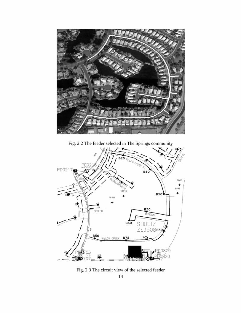
To study the residential microgrid system, The Springs community, located in
Chandler, Arizona, was selected and used as a test bed for the microgrid modeling, as
shown in Fig. 2.1. The feeder selected in The Springs community is 12.47 kV, single
phase supplied by 9 transformers with a total rating of 475 kVA, demarcated by a white
line in Fig. 2.2. Eighty-one houses are supplied with electric power by this feeder. The
circuit view of this feeder is shown in Fig. 2.3. It is found that the feeder is connected by
two power distribution cabinets PD-0217 and PD-0705GOS at the two ends. Nine trans-
formers are connected in series by this feeder with the individual unit capacity ranging
from 25 kVA to 75 kVA.
Fig. 2.1 The Springs Community
14
Fig. 2.2 The feeder selected in The Springs community
Fig. 2.3 The circuit view of the selected feeder

15
2.2 Energy Infrastructure Modeling
2.2.1. Computer-based software
HOMER, the optimization software developed by the National Renewable Energy
Lab (NREL), was selected and used throughout this work as a tool to design the mi-
crogrid for The Springs community. This software can model multiple DERs, such as
fuel cells, microturbines, PV, wind turbines, diesel generators, batteries, primal load, and
thermal load.
HOMER can simulate the hourly performance of one micropower system config-
uration to determine its technical feasibility and life-cycle cost; optimize system configu-
ration with the lowest life-cycle cost; conduct sensitivity analysis to check the effects of
variations in the model inputs [43].
2.2.2. Electrical system model
The feeder selected in The Springs community is connected by 9 transformers
with a total rating of 475 kVA. Eighty one houses are provided with electrical power by
these 9 transformers, and thus the average rating of a single house is 5.86 kVA. If a pow-
er factor of 0.8 is assumed, then the maximum electrical power provided by these trans-
formers is 380 kW.
In order to model an electrical load in HOMER, the hourly load profile of a day
(24 hours) along with an estimation of the Day-To-Day Random Variability and the
Hour-To-Hour Variability must be provided. Thus, an hourly dynamic residential load
profile of the 81 homes was used to model the electrical load of the selected feeder in The
Springs community. Meanwhile, a scale factor of 104% was applied to the hourly load

16
data to account for reactive power losses for these 81 homes. The average hourly power
demand in January is shown in Table 2.1 as a sample to represent the primary load input
in HOMER. The monthly load profile is shown in Fig. 2.4.
Table 2.1 Average Hourly Power Demand for 81 Homes in the Springs Community
Hour Real Power Demand (kW) Scaled Primary Load (kW)
0:00-1:00 99.363 103.337
1:00-2:00 89.723 93.312
2:00-3:00 85.496 88.916
3:00-4:00 83.494 86.834
4:00-5:00 84.506 87.886
5:00-6:00 91.277 94.929
6:00-7:00 106.783 111.054
7:00-8:00 116.848 121.522
8:00-9:00 113.370 117.905
9:00-10:00 113.085 117.608
10:00-11:00 113.471 118.009
11:00-12:00 113.985 118.544
12:00-13:00 112.889 117.405
13:00-14:00 111.536 115.997
14:00-15:00 109.965 114.363
15:00-16:00 112.565 117.067
16:00-17:00 122.792 127.703
17:00-18:00 151.712 157.780
18:00-19:00 167.793 174.505
19:00-20:00 169.308 176.081
20:00-21:00 166.546 173.208
21:00-22:00 155.743 161.973
22:00-23:00 136.676 142.143
23:00-24:00 114.785 119.376
The Day-To-Day Random Variability is estimated by:
1. Calculate the average real power demand for each day of 362 days,
2. Find the mean and standard deviation of the daily averages, and
3. Take the ratio of the standard deviation to the mean.
The Hour-To-Hour Variability is estimated by:

17
1. find the 24 hourly averages and the 24 hourly standard deviations of 362 days,
2. take the ratio of each standard deviation to its corresponding mean, and
3. take the average of the above ratios.
The results of the Day-To-Day Random Variability and the Hour-To-Hour Varia-
bility were thus calculated to be both 20%, and this data was used to model the daily and
hourly electric power noise.
The average daily load was calculated to be 3144 kWh for 81 homes. The average
and the peak power of this electrical load were calculated to be 131 kW and 480 kW, re-
spectively. The load factor was 0.273.
Fig. 2.4 Monthly load profile
2.2.3. Thermal load model
According to the data from the City of Chandler, average daily water use is 136
gallons per person in Chandler. For 81 homes with 3.2 persons per home, the total daily
water consumption is 35251 gallons. Salt River Project (SRP) estimates that 30% of the
residential water usage is heated and about 13% of household energy use is for water
heating. The average daily electric power consumption is 3144 kWh for 81 homes. Thus,
the hot water consumption and energy consumed for heating the water for these 81 homes
are 10576 gallons per day and 409 kWh per day, respectively.

18
2.2.4. The grid model
The grid model is used to model the performance of the microgrid in The Springs
community in grid-connected mode. The rates information is made publically accessible
through SRP. Considering the real conditions of the residents in Chandler, the Basic Plan
[44] was selected as the rate schedule.
The electricity sold back to the grids was assumed to be $0.09/kWh, and the net
purchases calculated monthly were applied. The emissions factors [45] for grid power are
shown in Table 2.2.
Table 2.2 Emissions Factors for Grid Power
Parameter (g/kWh) The Springs Value Default HOMER Value
Carbon Monoxide 526 632
Unburned Hydrocarbons 0 0
Carbon Monoxide 0 0
Sulfur Dioxide 0.476 2.74
Particulate Matter 0 0
Nitrogen Oxides 0.733 1.34
2.3 Microgrid Components Design
2.3.1. PV model
One programmed Excel calculating sheet was developed to determine the PV sys-
tem sizing. Three kinds of modules, PV-UE125MF5N from Mitsubishi, SW165-Mono
and KD135GX-LP from Kyocera, were selected [46].
Google Earth software was used to help determine houses qualified for roof-top
set-up of PV modules. For the 81 houses supplied by the selected feeder, the individual
room azimuth angle was firstly measured with the ruler function of Google Earth and this
angle must be ensured in the range of 135 to 225 degrees or (-45 to 45 degrees). Only at

19
these angles can the PV modules sufficiently utilize the sunshine energy to maximize
power production.
For houses with roof azimuth angle in the range of 135 to 225 degrees, the roof-
top area was calculated by measuring the length and width or equivalent area for irregular
roofs with the help of ruler function. The tilt angle of roof-mounted PV modules was as-
sumed to be 15 degrees. The exploitation factor of the roof area was assumed to be a rea-
sonable value of 0.85, meaning the entire roof area cannot be fully utilized due to con-
straints such as chimneys, skylights, or air conditioning units. The real available roof area
is the product of the initial total roof area measured by Google Earth multiplied by the
exploitation factor over the cosine of the tilt angle.
After these two steps, 32 out of 81 houses were selected according to the limita-
tions placed by azimuth angle and roof area. In total 1309 modules can be placed on the
combined roof area of the 32 selected homes.
DC rating of the PV system
The maximum number of modules was calculated by dividing the real roof area
by individual module area. If the number of modules per string is assumed in the range of
6 to 15, then the maximum number of strings is reached. Therefore, the total number of
modules is the result of the number of modules per string multiplied by the maximum
number of strings. The number of actual modules is largest value in total modules with
modules per string from 6 to 15. The total DC rating is the result of the peak power of
each individual module multiplied by the calculated number of actual modules. For this
case, the total DC output was calculated as 147 kW.

20
AC power output
PVWATTS [47], a performance calculator for grid-connected PV systems, was
used to determine the AC energy output of the PV system. For this study, PVWATTS
version 1 was used.
Firstly, the US location and the AZ territory was selected sequentially. Four plac-
es were then listed: Flagstaff; Prescott; Phoenix; and Tucson. The PV system specifica-
tions were loaded by clicking on Phoenix, and the value of DC Rating was changed ac-
cording to the calculation.
Table 2.3 Overall DC to AC Derate Factor
Component Derate Factors Derate Values Acceptable Range
Module Nameplate DC Rating 0.98 0.80-1.05
Inverter and Transformer 0.92 0.88-0.98
Mismatch 0.98 0.97-0.995
Diodes and Connections 0.995 0.99-0.997
DC Wiring 0.99 0.97-0.99
AC Wiring 0.99 0.98-0.993
Soiling 0.96 0.30-0.995
System Availability 0.98 0.00-0.995
Shading 1.00 0.00-1.00
Sun-tracking 1.00 0.95-1.00
Age 1.00 0.70-1.00
Overall DC to AC Derate Factor 0.81
The value of DC to AC derate factor was calculated as shown in Table 2.3. The
Array Type was selected as Fixed Tilt and the Array Tilt was fixed at 15 degrees. The
Array Azimuth was changed according to the measurement of every qualified house.
The solar radiation of Phoenix, AZ, is shown in Fig. 2.5. The final output AC en-
ergy of PV modules for these 32 houses was calculated to be 256772 kWh a year, as
shown in Fig. 2.6.

21
Cost of PV system
By the time of this study, the price of Mitsubishi PV modules was as low as $400
for each PV module. Thus, the total cost of PV modules for these 32 houses was calculat-
ed as $523600. The module cost typically represents only 40-60% of the total PV system
cost. Therefore, the total cost for this PV energy system would be about $872667, includ-
ing the total cost of cabling and installation.
Fig. 2.5 Solar radiation in Phoenix, AZ
Fig. 2.6 PV Output AC energy for 32 houses

22
According to SRP incentives [48], for residential units which installed a solar
electric system in Arizona, SRP would reduce the cost with an incentive of $2.7 per watt,
up to $13500 (through April 30, 2010). The Arizona tax credit accounted for 25% of the
cost, up to $1000. The federal tax credit accounted for 30% of the cost minus the SRP
incentive. Thus, the final net cost after credits and incentives was calculated as $353345
for 32 houses. The final average cost was $2.251/watt.
2.3.2. Microturbine model
C65-ICHP MicroTurbine [49], manufactured by Capstone INC., was selected as
one distributed generation source. The rating electrical power output and the rating ther-
mal output are 65 kW and 120 kW, respectively.
Table 2.4 Real Electric Output of Microturbine C65
Ambient Average Temperature ( ) Maximum Electric Output (kW)
Summer (81.8) 56.9
Summer Peak (92.5) 53.3
Winter (60) 65
Annual Average (72.6) 60.6
Table 2.5 Real Thermal Output of Microturbine C65
Ambient Average Temperature ( ) Maximum Thermal Output (kW)
Summer (81.8) 111.5
Summer Peak (92.5) 108.3
Winter (60) 111.4
Annual Average (72.6) 111.7
The real electrical and thermal output displays a correlation with local ambient
temperature, ambient elevation, inlet water temperature, inlet water flow rate and the wa-
ter column backpressure. After taking all of these factors into consideration, the final real

23
electric output and the final real thermal output provided by C65 microturbine (1117 feet
elevation, 4 inch WC backpressure, 140 (60 ), 40 gpm (2.5l/s)), are shown in Table
2.4, and Table 2.5.
Hot water model
The exhaust heat of microturbines is recovered to provide the hot water for the
residents for air conditioning, heating, cooking, cleaning, bathing, washing and laundry.
The microturbine C65 can work as a tankless water heater. In order to handle a full house
load of multiple uses, the hot water flow rate of 40 gpm was assumed. The daily hot wa-
ter demand can be found by using the volumetric flow rate, as shown in (2.1):
(2.1)
The hot water demand was finally modeled according to the time periods, as
shown in (2.2):
{
(2.2)
The time producing the hot water was calculated as 4 hours per day. The hot wa-
ter demand for the residents daily use is met by letting the running water go through mi-
croturbines that operate in standard conditions for an hour after each 5-hour interval.
Moreover, a hot water tank with a capacity of 2650 gallons (one fourth of the dai-
ly hot water consumption) or larger is suggested to hold the generated hot water. A five
percent Day-To-Day Random Variability and Hour-To-Hour Random Variability was
applied to account for the unknown daily and hourly variations.

24
The calculated average thermal load was 446 kWh/day, and the load factor was
0.132. The peak load is 141 kW. The thermal load is relatively more constant than the
electric load.
Microturbine fuel system model
Natural gas is provided as the fuel for the microturbine C65. The monthly Arizona
price of natural gas delivered to residential consumers from 1989 to October 2009 is
shown in Fig. 2.7, which presents an overall trend of increasing prices with time, about
five percent every four years. For this study, the natural gas price was assumed to 0.84
$/m3
(23.75 $/mcf), and the sensitivity analysis of natural gas price will be discussed in
next chapter. The fuel parameters used in this Microgrid design of The Springs communi-
ty are the default HOMWER values.
Fig. 2.7 Monthly Arizona price of natural gas delivered to residential consumers
Emissions and economic models
The emission factors of the microturbine C65 under full load condition are shown
in Table 2.6.

25
Table 2.6 Microturbine C65 Full Load Emission Factors
Parameter (g/m3) The Springs Value Default HOMER Value
Carbon Monoxide 0.0111 6.5
Unburned Hydrocarbons 0.00141 0.72
Particulate Matter 0 0.49
Nitrogen Oxides 0.019 58
Table 2.7 Microturbine C65 Cost Parameters
Parameter Capital Cost
($)
Replacement
Cost ($)
O&M Cost
($)
Lifetime
(hours)
Microturbine C65 100000 90000 0.013 175200
The cost data of microturbine C65 are shown in Table 2.7. All the data were
achieved from the consultation with the distributors of Capstone INC. and relevant tech-
nical reference [50].
2.3.3. Fuel cell model
The GenSys Blue fuel cell [51] manufactured by PLUG POWER INC. in New
York was selected as another distributed generation resource for the residential applica-
tions. This type of fuel cell can transform low cost natural gas into high value electricity
while generating usable heat and hot water.
For the residential fuel cell marketed by the Plugpower Inc, there is a federal tax
credit of 30% of the cost for the fuel cell or up to $3000 per kW, which expires on De-
cember 312016. The GenSys Blue residential fuel cells are still in precommercial phase,
and thus their price is quite high, at about $125000 for a 5kW fuel cell. The cost esti-
mates for the fuel cell system are based on manufacturers’ target price estimates rather
than actual purchase prices. The estimates should be considered to be within a range of -

26
25% to 25% [50]. The relevant cost estimates of the GenSys Blue 5kW fuel cell are
shown in Table 2.8. The parameters of the emissions model of the 5kW GenSys Blue fuel
cell are referred to [50] and [51], as shown in Table 2.9.
Table 2.8 Estimates of the Fuel Cell System Cost
Size (kW) Capital ($) Replacement ($) O&M ($/hr)
5 47500 28500 0.023
Table 2.9 Emissions Input of Fuel Cell
Parameter (g/m3) The Springs Value Default HOMER Value
Carbon Monoxide 0.0185 6.5
Unburned Hydrocarbons 0.00141 0.72
Particulate Matter 0 0.49
Nitrogen Oxides 0.021 58
Fig. 2.8 VRB battery inputs

27
2.3.4. VRB battery
The Vanadium Redox Battery technology is marketed by Prudent Energy Inc, a
Canadian company. The VRB battery was chosen as the energy storage for the microgrid
design for The Springs community. Compared with lead-acid batteries, the VRB battery
has many advantages, as shown in Table 2.10.
The cost of cell stacks and the cost of electrolyte and their corresponding size are
the results of consultation with some technical staff from the Prudent Energy Inc. A
screen shot of the inputs of the VRB battery is shown in Fig. 2.8:
Table 2.10 Comparison of VRB Battery with Lead-Acid Batteries [52]
Parameter Lead-acid Batteries VRB Battery
Energy Density(Wh/L) 12-18 16-33
Power Density (W/kg) 370 166
Efficiency (%) 45 65-75
Charge to Discharge ratio 5:1 1.8:1
Depth of Discharge (DoD) (%) 20-30 75
Life Cycle (discharge to 75% DoD) 1500 10000
2.4 Methodology Description
The flow chart of the optimization algorithm is shown in Fig. 2.9. Industrial,
commercial, as well as environmental data were collected, analyzed and applied as the
input for models built for the subsystems.
Based on the electrical and thermal load in this community, the search space for
each optimization unit was assumed and specified. The number of possible system con-
figurations is the product of all values in the search space for each optimization unit.
A total of 36000 simulations were run and the overall winning value for each sys-
tem component was selected. The above overall winner of variable for each system com-

28
ponent was determined under the assumption that all components worked at full capacity.
However, this is not always the case in the real world since some components in the sys-
tem may operate in the partial load condition. Therefore, one more approximate value for
the overall winner of each component was needed. The search space was refined each
time after the simulation until the optimal system configuration was found. The optimal
system configuration was sorted out by comparing the cost of energy (COE) and net pre-
sent cost (NPC).
Obtain industrial, commercial,
and environment data
Set the search space for
each optimization unit
Search space is sufficient
No
Optimal system
configuration
Yes
Set values for sensitive
variables concerned
Build the model
Run optimization
process
Sensitivity analysisYes
No
Fig. 2.9 Optimization algorithm flow chart

29
2.5 Microgrid Configuration
The optimal microgrid system configuration was determined as follows:
Microturbine capacity: 270 kW (five Capstone Microturbine C65 considering
the real electric output in Phoenix )
PV capacity: 157 kW (the maximum available DC output of the PV modules)
VRB-ESS battery rating: 100 kW
VRB-ESS storage: 400 kWh (cycle charging)
Converter: 300 kW
The categorized optimization results of all possible microgrid system configura-
tions are included in Fig. 2.10, from which for the most optimal system configuration the
total NPC is found to be $4264314; COE is $0.336 per kWh, and no fuel cells are includ-
ed in this kind of microgrid system configuration.
Fig. 2.10 Categorized optimization results

30
CHAPTER 3.
RESULTS ANALYSIS OF RESIDENTIAL MICROGRID DESIGN
3.1 Results Analysis
3.1.1. Economics
For this analysis, a life time of 25 years for this project was assumed. The nomi-
nal cash flow of the annual costs over the 25 years is shown in Fig. 3.1. A real interest
rate of 8% was assumed to calculate the NPC of the microgrid system designed for The
Springs community. The discounted cash flow diagram is shown in Fig. 3.2, which shows
the discounted cash flow of the present value for future costs of the designed microgrid
system. From these two figures, it is found there is no cash flow in during the 25-year
project period; the main cost of the designed residential microgrid is the large amount of
initial investment and yearly fuel cost thereafter. The cost in the 15th year is the replace-
ment cost of the flow battery and converter, while the cost in the 25th year is the salvage
cost of microturbines, the flow battery and the converter.
Fig. 3.1 Normal cash flow diagram for The Springs microgrid system
31
Fig. 3.2 Discounted cash flow diagram for The Springs microgrid system
3.1.2. Electrical output
Table 3.1 Electric Output Summary
Production kWh/yr %
PV Module 326566 27
Microturbine C65 894064 73
Total 1220630 100
Consumption kWh/yr %
AC Primary Load 1147355 100
Total 1147355 100
Quantity kWh/yr %
Excess Electricity 4462 0.366
Unmet Electric Load 205 0.018
Capacity Shortage 1014 0.088
Quantity Value
Renewable Fraction 0.137
The detailed information about the electric output is shown in Table 3.1. It is clear
from Table 3.1 and Fig. 3.3 that the microturbines provide the most electricity due to
their higher capacity and the fact that they can work continuously through a 24-hour cy-

32
cle according to real needs, while the PV modules can only work when there is sunshine
available.
Moreover, only 32 out of 81 homes are qualified for PV installation and 137 kW
DC output is the maximum electrical power supplied by the PV system. The real output
of PV modules is vulnerable to weather factors. July and August is the peak of summer in
Phoenix; electric production during these two months, in addition to September, is much
larger than the remaining months. This is due to the large load in air conditioning usage
during the hot summers of Phoenix.
Fig. 3.3 Monthly average electric production
3.1.3. Thermal output
As shown in Fig. 3.4, microturbines provide most of the thermal demand. The
boiler is used as the backup when microturbines and PV modules do not work. The boiler
can use the grid electricity or excess electricity generated by microturbines and PV mod-
ules to directly heat the water, or use the electricity provided by the batteries.
The thermal load can be used for cooking, bathing, space heating, showers, wash-
ing and laundry purposes. From Table 3.2, the thermal load of 162790 kWh/yr is met by
operating microturbines in full load with running water passing through 4 hours each day.

33
Considering the load change in real terms, this time could be longer than 4 hours. The
maximum thermal output could be reached if the running water was continuously provid-
ed to the microturbines as long as they were working.
Fig. 3.4 Monthly average thermal production
Table 3.2 Thermal Output Summary
Production kWh/yr %
Microturbine C65 1133013 97
Boiler 32167 3
Total 1165180 100
Consumption kWh/yr %
Thermal Load 162790 100
Total 162790 100
Quantity kWh/yr %
Excess Thermal 1002390 616
The excess thermal output is used to drive the adsorption chillers to provide the
cooling demand for the residents. The air conditioning load for 81 homes is approximate-
ly 573780 kWh/yr. One or several adsorption chillers with coefficient of performance
(COP) above 0.57 will satisfy this cooling demand. If an average of 2.6 tons cooling ca-
pacity for each home is assumed, then the total air conditioning capacity is about 210 tons.
Commercial chillers [53] are available with capacities from 10 to 1000 tons of refrigera-
tion.

34
3.1.4. PV performance
PV production usually occurs between 6:00 am to 18:00 pm when the sunshine is
available at most times. Also, the most PV output happens after noon between 13:00 pm
and 15:00 pm when the intensity of the sun’s radiation is the strongest. In Fig. 3.5, note
that usually July is the hottest month throughout the year in Phoenix, AZ, but the PV out-
put is not correspondingly the largest. This results from high surface temperatures of the
PV modules thereby reducing the efficiency of sunshine energy conversion.
Fig. 3.5 PV modules power output monthly averages
3.1.5. Microturbine performance
Fig. 3.6 Microturbine electric output monthly averages
The microturbines provided 73% of the electric energy. The hourly electric output
of the microturbines shows that they do not always operate in full load; the least power
was produced between 9:00 am and 16:00 pm except in July, August and September due
to increased load demand for air conditioning use in Phoenix during the summer months.

35
The most power was provided between 16:00 pm and 24:00 pm during July, August and
September when most residents are at home during this period. Fig. 3.6 also shows that
both the daily high electric output and daily low electric output in July, August, and Sep-
tember are larger than the other months.
3.2 Grid-connected Mode
The simulations towards the microgrid configuration in grid-connected mode
were conducted for comparisons with the standalone microgrid configuration. The cate-
gorized simulation results are shown in Fig. 3.7, which illustrates that for the optimal mi-
crogrid system configuration, no microturbines, fuel cells or PV modules are included;
COE is $0.091 per kWh, and the total NPC is $1794928, approximately 1.4 times less
than that of the most optimal microgrid configuration in the standalone mode. In this case,
residents are actually purchasing electric energy from the grids.
Fig. 3.7 Categorized simulation results in grid-connected mode

36
The emissions factors of both microgrid systems are shown in TABLE 3.3. This ta-
ble indicates that the grids produced about 114 tons of carbon dioxide more than that of
the standalone microgrid system. Moreover, the nitrogen oxides produced by the grids are
133 times more than that produced by the standalone microgrid system, while the latter
system produced 1.8 times of sulfur dioxide as much as that of the former system. Thus,
the designed standalone microgrid system for The Springs community is more environ-
mentally friendly than the grid system.
Table 3.3 Emissions Factors of Both Systems
Standalone microgrid Grids
Pollutant Emissions (kg/yr) Emissions (kg/yr)
Carbon dioxide 636597 750374
Carbon monoxide 3.73 2.84
Unburned hydrocarbons 0.474 0.361
Particulate matter 0 0
Sulfur dioxide 1710 941
Nitrogen oxides 6.38 846
3.3 Sensitivity Analysis
From the economic analysis, the initial investment of the DERs and the yearly
fuel cost seem to play a vital part in NPC and COE. It was hypothesized that the natural
gas price escalation and the price reduction of DERs had the most significant effect on
NPC and COE. This hypothesis is verified through the following sensitivity analysis.
The COE and the NPC goes down linearly with the price reduction of PV and mi-
croturbines. The effect of the fuel cell price reduction on COE and NPC at the natural
price of $0.84/m3 is shown in Fig. 3.8. When the fuel cell (FC) multiplier is smaller than
0.8, the FC price begin to influence COE and NPC clearly, while the COE and NPC re-

37
main unchanged for a constant MTC65 capital multiplier until the FC multiplier is small-
er than 0.73.
Fig. 3.8 FC capital multiplier vs. microturbine capital multiplier
The COE and NPC go up linearly with an escalation in the price of natural gas.
The effect of natural gas price escalation and the fuel cell price reduction on COE and
NPC is shown in Fig. 3.9. There is little difference between NPC and COE responses to
changes in natural gas price escalation with the PV and MTC65 capital multiplier. For a
constant natural gas price, there is no change in COE and NPC until the FC capital multi-
plier is smaller than 0.8. The natural gas price affects NPC about $400K for a natural gas
price delta of 0.1$/m3.

38
For all cases, the general trend of COE and NPC goes down with price reductions
in the DERs, and goes up linearly with natural gas price escalation. The price of the
DERs has more weight than that of natural gas in determining COE and NPC. For the
conditions set in this sensitivity analysis, the lowest COE and NPC is 0.3$/kWh and
$3846073, respectively, which happens when the price of microturbines and fuel cells
reduces to a half and the fuel cell price remains constant at the natural gas price of
0.84$/m3.
Fig. 3.9 Natural gas price vs. FC capital multiplier

39
3.4 Water and Natural Gas Availability
3.4.1. Water availability
A 36-inch water pipeline runs along McQueen Rd, as shown in Fig. 3.10. It is ca-
pable of moving more than 90 million gallons of potable water per day (62500 gpm). The
water mains that run along the streets in the neighborhood are 6 inches in diameter with a
water delivery flow velocity of 4.7 ft/s. The static pressure is assumed to be 45 pounds
per square inch gauge (psig). Thus, the water capacity of the water mains is calculated to
be 0.0261 m3/sec (414 gpm). The water consumption of the 81 homes is 35251 gal-
lons/day (24.48 gpm).
Fig. 3.10 Layout of the water pipe line

40
The minimum working pressure for water distribution pipes is approximately 100
psig at 180 (80 ) by the gauge [54], and this pressure is reduced with the friction
head loss. It is found that when the water flow rate is 40 gpm, the velocity of water flow-
ing rough the 2 inches line is calculated as 4.08 ft/sec, less than the maximum allowed 5
ft/sec and at this rate the water head loss is about 1.01 psig/100 ft due to the supply line
friction. The resultant pressure at the inlet of the microturbine would change little. A reg-
ulator is used to reduce this pressure to be acceptable for microturbine or fuel cells.
The basic pipe flow equation is shown in (3.1):
Q V A (3.1)
which can be converted to the following equation with normal units of measure and the
inside pipe diameter.
22.448Q V D (3.2)
As for the microturbine C65, the rating inlet water flow rate is 40 gpm, and the in-
let water pipe diameter is 2 inches. Thus, the inlet water velocity of the microturbine was
calculated as 4.08 ft/s (40 gpm rating inlet water flow rate). Thus, the existing water dis-
tribution system provides sufficient water for five microturbines, and the water consump-
tion of five microturbines and 81 homes accounts for 54.22% of the water mains capacity.
The Capstone C65 microturbine is air-cooled, and thus it doesn’t need any cool-
ing water to cool down itself. The inlet water is just used to utilize the heat from the ex-
haust of the Capstone C65 microturbine and improve the total system efficiency. Thus,
there are actually not any rigid requirements for the inlet water. As long as the inlet water
goes through the microturnine, the hot water will come out of the microturbine. The rat-

41
ing water demand for each Capstone C65 microturbine is 40 gpm and the rating inlet wa-
ter temperature is 140 (60 ). These values are just guaranteed to make sure that the
thermal output is 112 kW. In reality, correction factors about inlet water temperature,
flow speed, and column backpressure, are considered when calculating the final thermal
output.
3.4.2. Natural gas availability
Fig. 3.11 Layout of main gas line
The gas main in The Springs community, as shown in Fig. 3.11, only goes
through a portion of the 81 homes with a diameter of 2 inches at 60 psig. The nearest

42
regulator station is at the northeast corner of McQueen Rd & Ray Rd with a present ca-
pacity of 101.23 thousand cubic feet per hour (mcfh) and 69.699 mcfh for the worst case
scenario for cold temperatures in a 28 heating degree day cycle. For the microturbine, the
inlet pressure is 74-80 psig; the rating fuel flow is 842000 Btu/hr (765.45 cfh). For five
microturbines, the total gas usage is 3827.25 cfh. The present capacity of the gas main
will be sufficient to provide this amount of gas through five branch lines (2-inch diameter
and with lengths between 20 to 200 ft). The gas pump is required to increase the inlet gas
pressure of microturbines to the rating range.
3.5 Conclusions
This report investigates the design methods of a residential microgrid infrastruc-
ture by building a comprehensive model and evaluating the simulation results. No fuel
cells are found in the optimal residential microgrid system configuration due to high ini-
tial investment and low capacity. More detail about the economic feasibility of a residen-
tial fuel cell can be found in [55]. PV seems to be a good choice in the design of residen-
tial microgrid infrastructure, especially considering the incentives and credits from gov-
ernments and states and the reduced prices of PV raw materials. The combination of mi-
croturbines and adsorption chillers plays a vital part in fulfilling the goal of CCHP.
The sensitivity verifies that COE and NPC are mainly affected by the initial pro-
ject investment and yearly fuel cost. When the fuel cell price drops below 0.8 times of its
original price, COE and NPC becomes more affected by the fuel cell price and goes up
linearly with an increase in natural gas price. The natural gas price affects NPC about

43
$400K for a natural gas price delta of 0.1$/m3. The designed residential microgrid infra-
structure is sustainable and environmental friendly compared to the grids.
3.6 Extension Work
The test bed in The Springs community is just a section of a small feeder supply-
ing 81 households. The research work conducted for this test bed investigated selections
and behaviors of DERs based on economic concerns, sensitivity analysis and energy bal-
ance for part of the design work of a residential microgrid, from which the designed mi-
crogrid configuration was determined. Further investigation was also conducted to identi-
fy the availabilities of natural gas and water for supporting the normal operation of some
DERs in existing residential energy infrastructures.
Fig. 3.12 Phoenix downtown area
The problem for this method is that if the test bed size is increased, like the Phoe-
nix downtown area surrounded by I10 and I17 freeways, as shown in Fig. 3.12, the essen-

44
tial concerned problems are that in this area, how much DG can be placed and where to
put these DERs based on existing energy infrastructures, and what’s the mutual impact on
operational performances between DERs and energy infrastructures. For these problems,
the above mentioned method is not applicable to solve these problems for a larger system.
In this case, a more systematic as well as generalized methodology should be developed
to solve these problems. In remaining chapters, one comprehensive mathematical model
will be developed step by step to help solve the above mentioned problems.

45
CHAPTER 4.
ELECTRICAL SYSTEM MODEL DEVELOPMENT
This chapter presents how the electrical system was selected, modified, and mod-
eled according to requirements as well as some reasonable assumptions.
4.1 Electrical System Selection
The electrical system selected has to be a distribution system such that the urban
environment is guaranteed and all other energy infrastructures studied should also be at
the distribution level. For this work, the electrical system was determined first, then the
gas and water distribution networks were developed corresponding to this electricity net-
work, all of which compose the basic urban energy infrastructures.
The Phoenix downtown area, surrounded by Roosevelt St in the North, Lincoln St
in the South, N 7th Ave in the West and N 7th St in the East, was first selected as the
study area. However, only three feeders’ data were provided with insufficient information
by Arizona Public Service (APS). In addition, this area is supplied with electricity by
over ten feeders from nearby substations of APS and Salt River Project (SRP). Lacking
of enough and complete data, the real test bed plan was abandoned.
Since in the rest chapters, one generalized integrated system model would be de-
veloped, the IEEE 123 node test feeder [56] was selected as the electrical system for this
study, as shown in Fig. 4.1. This is because that this system has been already complicated
enough as a distribution system feeder and enough electrical data are provided. In addi-
tion, this test feeder is actually extracted from some real distribution system. Therefore, it
can be used to represent the real system feeder.

46
Fig
. 4.1
IE
EE
123 n
ode
test
fee
der

47
The system voltage level is 4.16 kV. The main feeder is three-phase overhead and
most lateral feeders are single-phase overhead feeders. Two two-phase overhead feeders
are also included. One substation transformer and one distribution step-down transformer
are connected by this feeder. There are also four voltage regulators as well as four shunt
capacitors included to improve the system voltage profile, either in three-phase or in sin-
gle phase. The loading of the feeder’s three phases is unbalanced and all loads are repre-
sented by spot loads, either Wye or delta connected with the feeder. The three-phase
switches between node 13 and 152, node 18 and 135, node 60 and 160, node 61 and 610,
node 97 and 197, node 150 and 149 are normally closed; while the rest switches are nor-
mally open.
4.2 Electrical System Modification
The selected electrical system is a typical radial distribution feeder such that there
is only one way of power flow. Since the given test feeder is only part of itself, the big
picture of this feeder is unknown without knowing the starting point and ending point.
Therefore, reasonable assumptions were made to change this radial distribution
system into a looped system. In this way, each load could be supplied by electric power
from two ways besides the introduced DERs such that the system reliability is much im-
proved. Meanwhile, the system maximally accommodated DG capacity is also increased
compared to the radial system, which has already been identified in an early research
work conducted and contributed for this research topic [25]. These assumptions are the
followings: first, this radial feeder is connected at some points with other feeders or grids
of upper voltage level or substations; second, four AC power sources (ExGens) were

48
added and connected at nodes 149, 300, 450, and 95, to represent other systems connect-
ed to this feeder, as shown in Fig. 4.2.
By adding these AC power sources, a looped system is formed. The original radi-
al distribution feeder now is actually divided into several sections. Each section could be
a sub-feeder, which connects two AC power sources with one switch at each side of the
sub-feeder. When all these switches keep open, the looped system will change back to the
original radial system; when all or some of them close, a looped system is formed.
4.3 Individual System Phase Configuration
The modified system is still not a competely three-phase system, and only the
main feeder is in three phase. Two-phase feeders are also included. Therefore, the
traditional ACOPF model cannot be directly applied to this system. In this case, to make
the evaluation of results more accurate, the modified system is separated phase by phase,
which means that the original system is now represented by three individual systems.
The ACOPF formulation was then applied to each of these individual system and
the results achieved from each phase were then added up togher for each node, which
compose the final nodal electrical output. The individual system phase configurations are
shown in Fig. 4.3, Fig. 4.4, and Fig. 4.5, respectively.
4.4 ACOPF Formulation
The objective of the integrated system is to maximize the CHP-based DG output,
including both electrical output and recovered thermal output. Solely for the electrical
system, the objective is to maximize electrical output and corresponding thermal output.

49
Fig
. 4.2
Modif
ied l
ooped
syst
em

50
Fig
. 4.3
A p
has
e sy
stem
confi
gura
tion

51
Fig
. 4.4
B p
has
e sy
stem
confi
gura
tion

52
Fig
. 4.5
C p
has
e sy
stem
confi
gura
tion

53
It was assumed that a couple of CHP-based DG units were located at each node
with the capacity from zero to a set value, which is multiple times of the base unit’s ca-
pacity. This means that the DG electrical power output is treated as a continuous variable
with both lower and upper capacity bounds. In this case, the final real output will be de-
termined by the developed algorithm based on the electrical system. If the power output
is zero, then it means no CHP-based DG units are placed in that node. If the power output
is not zero, then one or several CHP-based DG units can be placed in that node according
to the units’ capacity availability and system connection requirements.
The actual maximum and minimum DG electrical and thermal capacities are mul-
tiple times of the selected base DG unit’s electrical and thermal capacities, which should
be changed according to the number of DG units connected at each node. The capacity
constraint for the CHP-based DG unit is shown in (4.1): , g G n N
( , ), ( , ) ( , ),
, , ,
E T E T E T
g n g n g nP p P (4.1)
The external AC power source supply constraints are shown in (4.2) and (4.3), re-
spectively: x X n N . Normally, these ExGens’ capacities are assumed at 50-60
MW in distribution systems.
, ,
, , ,
X X X
x n x n x nP p P (4.2)
, ,
, , ,
X X X
x n x n x nQ q Q (4.3)
The ExGens’ angles are set to zero, as shown in (4.4):
0x (4.4)

54
The nodal voltage deviation is set to 5% of the rating value. The voltage level
constraint is shown in (4.5): n N
n n nV v V (4.5)
Shunt capacitors are included in this ACOPF formulation to provide the voltage
profiles support and improvement. The capacity constraint is shown in (4.6):
c C n N
, , ,
C
c n c n c nC s C (4.6)
The real power flow constraints at both ends of a line are shown in (4.7) and (4.8),
respectively: l L
2
,A A B A B A Bl l l l l l l
A P
l l l lN N N N N N Nf G v v v G cos B sin
(4.7)
2
,A B
l l l l l l lB B A B A
B P
l l l lN N N N N N Nf G v v v G cos B sin
(4.8)
The reactive power flow constraints at both ends of a line are shown in (4.9) and
(4.10), respectively: l L
2
,A A B A B A Bl l l l l l l
A Q
l l l lN N N N N N Nsin cosf B v v v G B
(4.9)
2
,B A Bl l l l
B Al l
B Al
B Q
l l l lN N N N N N Nsin cosf B v v v G B
(4.10)
Each nodal output in the electrical system is constrained by both real and reactive
power balance equation. The power flows into a node, including the power from ExGens
and that from the DERs, have to be equal to the summation of the nodal load demand and
the power that flows out of the node, as shown in (4.11) and (4.12), respectively: n N

55
, , , ,
| | | |N N A Bx g l l
X E P P P
x n g n n l n l n
x X n g G n l L N n l L N
p p D f f
(4.11)
, , ,
| | |
, ,
| |
N N Nx g c
A Bl l
X E C
x n g n g c n
x X n g G n c C n
Q
n l n l n
l L N n l L N n
Q Q
q p tan s
D f f
(4.12)
The reactive power injection part from the distribution lines was not considered as
the shunt capacitance is too small and the distances between lines are short.
The distribution lines are constrained by the ampere capacity. The thermal con-
straints of lines are shown in (4.13) and (4.14), respectively: l L
2 2 2
, ,A P A Q
l l lf f F (4.13)
2 2 2
, ,B P B Q
l l lf f F (4.14)
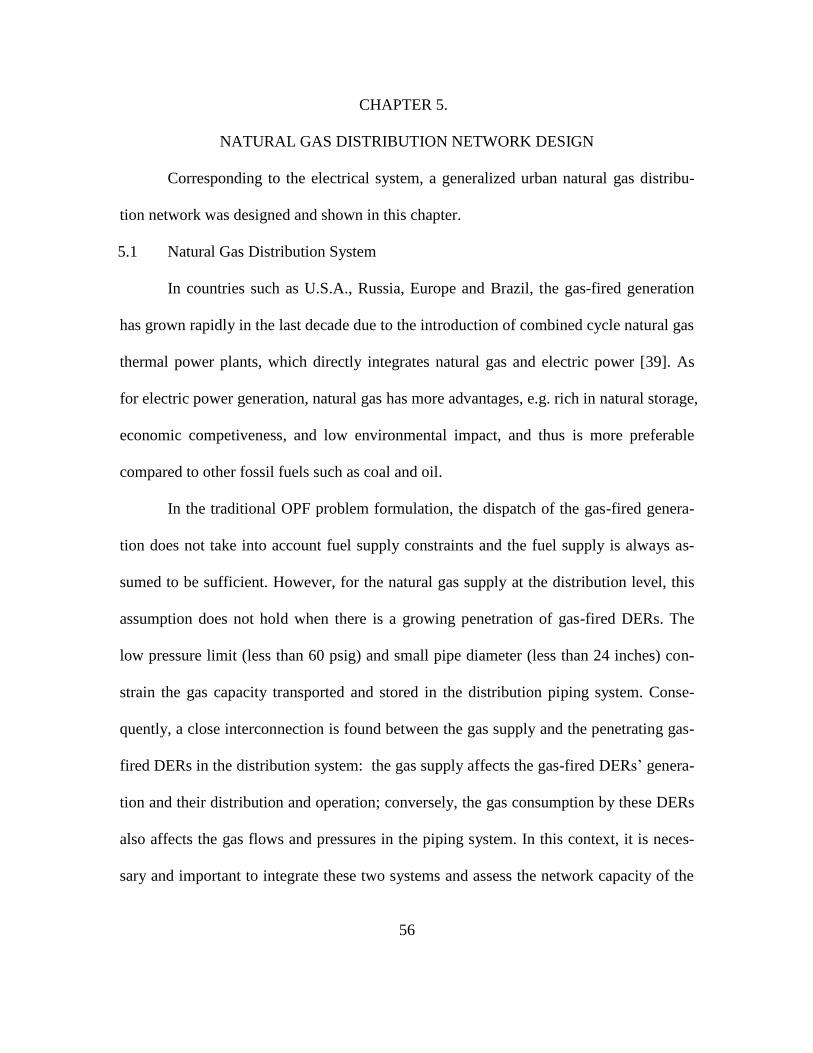
56
CHAPTER 5.
NATURAL GAS DISTRIBUTION NETWORK DESIGN
Corresponding to the electrical system, a generalized urban natural gas distribu-
tion network was designed and shown in this chapter.
5.1 Natural Gas Distribution System
In countries such as U.S.A., Russia, Europe and Brazil, the gas-fired generation
has grown rapidly in the last decade due to the introduction of combined cycle natural gas
thermal power plants, which directly integrates natural gas and electric power [39]. As
for electric power generation, natural gas has more advantages, e.g. rich in natural storage,
economic competiveness, and low environmental impact, and thus is more preferable
compared to other fossil fuels such as coal and oil.
In the traditional OPF problem formulation, the dispatch of the gas-fired genera-
tion does not take into account fuel supply constraints and the fuel supply is always as-
sumed to be sufficient. However, for the natural gas supply at the distribution level, this
assumption does not hold when there is a growing penetration of gas-fired DERs. The
low pressure limit (less than 60 psig) and small pipe diameter (less than 24 inches) con-
strain the gas capacity transported and stored in the distribution piping system. Conse-
quently, a close interconnection is found between the gas supply and the penetrating gas-
fired DERs in the distribution system: the gas supply affects the gas-fired DERs’ genera-
tion and their distribution and operation; conversely, the gas consumption by these DERs
also affects the gas flows and pressures in the piping system. In this context, it is neces-
sary and important to integrate these two systems and assess the network capacity of the

57
gas-fired generation based on the analysis of the integrated system operation, planning,
and reliability.
The designed gas piping system is a typical distribution system. However, it is al-
so necessary to understand generally how the whole gas system works including both the
gas transmission and gas distribution from the following steps [57]:
1. Natural gas typically comes from gas wells,
2. The gas from wells is then purified by removing sand, dust and water, and
odorized so that it can be easily detected,
3. The gas is usually compressed in underground storage fields in case of high
demand requirement during cold weather months,
4. The gas is pressured and pushed into storage and transmission lines by com-
pressor stations,
5. The pressured gas of 61 to 1000 psig is transported to the distribution system
via the transmission network,
6. Regulators are used to reduce the pressured gas entering the distribution sys-
tem to less than 60 psig,
7. Valves in the distribution system are only used to isolate certain gas pipelines
during construction and emergencies, and
8. The standard delivery pressure to residential customers is 1/4 psig.
5.2 Natural Gas Network Design
The software used to model the natural gas network is GASWorkS 9.0. The
GASWorkS 9.0 is a steady-state network modeling tool to analyze and design distribu-

58
tion, gathering, transmission, and plant piping systems containing natural gas or other
compressible fluids [58]. The node number of the designed gas network is more than 120,
which is beyond the node number limit of the demo version of this software. Upon the
request of the author, the distributor of this software agreed to offer one time-limited (4
months) free academic version of GASWorks 9.0 with no limit on the node number.
It was assumed that for spot load where the electricity was supplied, the natural
gas was also provided. Each node in the designed natural gas network corresponds to the
same node in the electrical system, which represents a cluster of houses. The base natural
gas consumption by these clustered loads was calculated by counting the households at
each node multiplied by the hourly natural gas consumption of individual household.
Based on the nodal electrical load, the nodal households can be counted and a total num-
ber of 1745 households were calculated for the area supplied with electricity and natural
gas. The per capita consumption of natural gas in Arizona homes in 2005 is 6.1 million
Btu [59]. Assumptions of 3.2 persons per household and an average usage time of 3 hours
per day were made. The average household consumption of natural gas was then calcu-
lated as 19.52 thousand cubic feet (mcf) one year and 17.83 cubic feet per hour (0.504
cubic meters per hour). Therefore, the total base natural gas load is 880.33 cubic meters
per hour for the designed natural gas distribution network.
There are many possible combinations of pipe material, diameters, valves, regula-
tors, etc., making the gas distribution network design a complicated process. To simplify
the whole network design, the smaller service lines of less than 1 inch in diameter are not
modeled in this network, which connect and provide gas for each individual house. Also,

59
the valves were not modeled in this network as they are only used to switch on or off the
gas supply of a certain area, especially during emergencies. The regulators are used in the
distribution system to reduce the output gas pressure and thus not modeled.
As for the pipe materials, the polyethylene (PE) plastic pipes were selected for all
pipelines as they are anticorrosive when buried underground, for which the metal pipe-
lines cannot substitute. At the distribution level, the gas pipeline diameters typically
range from a half inch to eight inches. Copper and iron are usually the pipe materials for
the pipelines of 0.5 inch in diameter. While for the pipelines of 2 inches to 8 inches, plas-
tic and steel materials are all found as the pipe materials. For this study, a series of differ-
ent diameters were selected to investigate the influence of gas supply to the operational
performance of gas-fired DERs.
The designed gas distribution network is shown in Fig. 5.1. The nodes in the gas
network correspond to the same nodes in the electrical network, which was used as the
background figure to determine the nodes’ coordinates. The thicker black lines in this
figure represent the plastic gas mains of 5.314 inches in diameter (inside) while the thin-
ner grey lines represent the plastic gas mains of 1.885 inches in diameter (inside). In ad-
dition, to improve the reliability of gas supply, the dashed lines were added to intercon-
nect the gas mains of larger diameter. In this way, the original radial system is now
changed into a looped system, and every customer could be supplied with gas in two
ways. The components of the transmission side in the gas system were omitted during the
design, such as well, compressor, and regulator. This is because that the focus of this
study is only on the distribution side after the gate station where the regulator locates.

60
Fig
. 5.1
Des
igned
nat
ura
l gas
dis
trib
uti
on n
etw
ork

61
The node 250 was designated as the supply node (city gate) of natural gas, for
which the pressure was fixed at 60 psig and the load is unknown and determined by run-
ning the simulation of the gas whole network. The downstream gas pressure after this
node in the distribution is below 60 psig. The elevation of all nodes and pipes in the gas
network was assumed in the same level everywhere. The ambient temperature was set to
70 When the gas flows through the system, it always flows from nodes with higher
pressures to nodes with lower pressures with the control of regulators, and the gas pres-
sure drops when flowing along the pipelines due to friction and gravity. Normally, the
further the gas load from the regulator or the supply node, the lower the gas pressure. The
gas pressure in the residential area is as low as less than 1/4 psig, which needs to be in-
creased by the natural gas compressor or booster inside the gas-fired DERs to ensure its
normal operation.
Multiple industry standard pipe flow equations are used to calculate the flow and
pressure drop in pipelines. It should be noted that each equation has its own unique char-
acteristics and limitations. The appropriate equation has to be determined for a specific
application. For the gas piping system designed in this study, it is a typical natural gas
distribution system consists of both high-pressure mains of up to 60 psig and low-
pressure mains of less than 1/4 psig, distributing gas from regulator stations to end users.
In this case, the IGT-Improved Equation [60] was selected and used in this application of
medium and high pressure distribution. It is applicable to all types of distribution systems
operating between 1 to 500 psig for two inch and larger diameter pipes, and yields mod-
erate results [61].

62
CHAPTER 6.
WATER NETWORK DESIGN AND MODEL DEVELOPMENT
Corresponding to the electrical system, a generalized urban water distribution
network was designed and its mathematical model was also developed in this chapter.
6.1 Water Network Design
The nodes in the water network designed are the same nodes in the electrical net-
work such that the CHP-based DERs could be used as the coupling point between these
two systems. Similarly, in the water network, each node was assumed to represent a clus-
ter of houses. The water demand was estimated based on the counted households at each
node in the water network and the nodal loading information in the electrical system. The
per capita average daily water use for a community in Chandler is 136 gallons [24]. The
water demand was then calculated by assuming an average usage time of 3 hours per day
per capita, and 3.2 persons per household for this study.
Numerous possible combinations of pipe material, diameters, pump capacities,
make water distribution network design a complicated process. Optimization techniques
are often used to obtain a design that best represents the interest of the stakeholders,
while in reality this may be not the case. Generic algorithms have proven to be successful
in dealing with such non-linear hard problems [62]. A genetic algorithm based optimiza-
tion tool (GANetXL) in combination with a hydraulic solver, EPANET, is used in this
research to design a representative water distribution network [63]. EPANET is a popular
water network solver that runs a water network simulation to obtain flows and pressures
at various points in the system [64].

63
The objective is to minimize the cost by choosing appropriate diameters. Various
pipe diameters available in the market are considered in the design. The pressure in the
system is constrained to be more than 60 psig or 42.2 m of water pressure head, which is
in the range of typical pressures expected in an urban water distribution system [65]. It
should be noted that the pressures in a water distribution system should be neither too
low nor too high. Low pressures, below 30 psig, cause annoying flow reductions with a
possibility of attracting contaminants into the pipe through leaks. Subsequently, pressures
less than 30 psig or 21.1 m of pressure head are considered unacceptable in this research.
High pressures may cause wear out in the system with a possibility of damaging system
components [65].
GANetXL in combination with EPANET was used to design the water distribu-
tion system by minimizing costs while maintaining minimum required pressures at all the
nodes in the system. The flowchart of this design process is shown in Fig. 6.1.
The basic idea in the flowchart is that: the pipe data from some database is used to
run the optimization of cost minimization based on GA. The resultant optimal pipe diam-
eters then update the water network database. Next, this optimal data is used to run hy-
draulic simulation. From the resultant nodal pressures, penalty is added depending on the
minimum node pressure criterion. Then, the results are saved and improved by redoing
this iteration process until the nodal pressure criterion is met.
The designed water distribution network corresponding to the electrical system is
shown in Fig. 6.2. Each node in the water network corresponds to the same node in the
electrical system. A reservoir is located in node 118 to provide all the water demand in

64
every node. The elevation of this reservoir is assumed to be 5 m. The water head pressure
drops when flowing in the pipelines due to the friction and gravity. Normally, the further
the water load from the reservoir, the lower the water head pressure in that load point. A
pump is connected between node 118 and node 250 to increase the water head pressure
up to the designed value (50 m) in node 250. This is also done to ensure that for all exist-
ing nodal water demand, the nodal pressure is above the minimum required water head
pressure. Two pressure reducing valves (PRV) are also included into this network to re-
strict the outflow not exceeding a set value. One is between node 8 and node 13; the other
is between node 67 and node 97.
Fig. 6.1 Flowchart of the water distribution system design [66]

65
Fig
. 6.2
Des
igned
wat
er d
istr
ibuti
on n
etw
ork

66
The designed water distribution network is a looped system. Each water demand
node is supplied with water by at least one pipe connected to that node, which increases
the reliability of the water supply for each node.
It also should be noted that in this designed water distribution network, there is
only one pump, located close to the reservoir. No other pumps exist in this system to
boost the water pressure. Therefore, in this case, the further the node from the pump, the
lower the nodal water head. This can be seen in the results analysis of Chapter 8.
6.2 Water Network Model Development
To better dynamically connect the water network and the electrical system, the
mathematical water network model was developed based on the designed water distribu-
tion network. In this case, the developed water network model will partially take the role
of EPANET and used for hydraulic simulation purposes.
To generate a pump equation, one point (1130 m3/hr, 45 m of water head) on the
pump curve was acquired by using EPANET. The pump equation is used to represent the
relationship between the head gain and water flow that a pump can deliver. The pump
adds pressure to the water head flowing out of the pump such that every nodal water
pressure head in the water distribution network is guaranteed to be above the required
minimum value. The following pump equation was achieved: p P b pump link
2
| |N A N B Bp b p b p
H H H Co F
MinDsgn pp N p Nw W W P w
(6.1)
where the unit of water pressure head is in meters and the unit of water flow is in cubic
meters per hour.

67
When water flows inside the pipeline, water pressure head drops along the pipe-
line due to the friction, as shown in (6.2) and (6.3) [67], b B , except the link where
the pump is connected in this water distribution network. In addition, the elevation of all
nodes and pipes were assumed as the same level except the reservoir such that the gravity
effect could be neglected in this study.
1.85
b bA B
H H F
bN
R
bNw w B w (6.2)
where the unit of water flow is in cubic feet per sec.
1.85 4.87
1.439R
b
HW
b bB C D L
(6.3)
where the Hazen-Williams roughness coefficient can be assumed as 130, the unit of link
diameter and length is in feet.
Typically, PRVs are used in water networks which work by not allowing water to
pass through at more than a set pressure. In this case, the downstream water pressure
head was set to not more than 60 m. If the upstream pressure is more than 60 m, the
PRVs reduce the downstream pressure to 60 m, as shown in (6.4) to (6.6) [67]: l L
| |60, 60N A N
v bB
v b
H H
v N v NIf w w
(6.4)
| | |60,N A N N A
v b v b v bB
H H H
v N v N v NIf w w w
(6.5)
24
| |31910 101.94 ( )N A N B B
v b v b v vB
H H F
v N v Nw w w D
(6.6)
where the unit of diameter is in mm.
The nodal balance equation [67] is also adaptable in the water system. The water
flows into a node equals to the existing water demand at that node plus the water flows

68
out of the node. The water used by the CHP-based DERs contributes additional water
demand to the total nodal water consumption: n N
, ,
| | | |N A B Nw b b g
W D
w n g n
w W n b B N n b B N n g G n
F F D
b b nw w Wr w
(6.7)
For each node, a range of acceptable water pressure head was set. The nodal water
pressure head should be within this range to ensure the normal supply of water, as shown
in (6.8): n N
H
n
H H
n nwW W (6.8)
For the CHP-based DG units, extra water will be used to carry away part of the
exhaust heat for thermal utilization purposes. A range of the required water flow is given
for units used for exhaust heat exploitation, as shown in (6.9): g G n N
, , ,
F D F
g n g n g nW w W (6.9)
.

69
CHAPTER 7.
THE CHP-BASED MICORTURBINE SYSTEM MODEL DEVELOPMENT
7.1 The CHP-based Microturbine System
The CHP-based microturbine system was developed and used as the coupling
point between electricity, gas and water networks. The diagram of the CHP-based micro-
turbine system is shown in Fig. 7.1.
Fig. 7.1 The CHP-based microturbine system
The natural gas is used as the fuel for microturbines. Biogas or the combination of
biogas and natural gas can also be used as the fuel for most gas-fired DERs. The electri-
cal output from microturbines and grids is used to supply the load with the extra electrici-
ty sold back to the grids. The thermal heat exhausted into the air can be recovered by the
water flowing inside the integrated or externally added heat exchanger, normally isolated
part or integrated part of microturbines, where the pressured water by the pump flows

70
inside. In case there is not enough hot water supplied, the boiler is usually added to pro-
vide extra hot water supply. A thermal storage, normally a water tank is necessary to
temporarily store the hot water as well as balance the hot water supply and demand. This
water flow process is a looped circulating process and a certain amount of water is taken
from the water network besides the normal daily water usage, which usually cannot be
drunk and is only one-time use. This is just the extra water used by the CHP-based DERs
to recover the exhaust heat.
The microturbine C65 was selected as a reference for the CHP-based DERs. The
capacities of these series of products are available in a wide range, which can be modu-
larized and show similar electrical and thermal characteristics as this selected unit.
7.2 Mathematical Formulation
As for the modeling of the CHP-based microturbine system, only the influences
of water flow speed, sending and returning water temperature, and ambient temperature
are considered to simplify the optimization process. The pump, thermal storage, and boil-
er were not key parts in the integrated whole system, and thus not modeled in this study
since they will significantly complicate the whole optimization process and make the cal-
culation much slower by introducing binary variable for the boiler. In that case, the whole
model will be changed from a nonlinear nonconvex problem into a mixed integer nonlin-
ear nonconvex problem, which is very hard to solve and the results’ accuracy cannot be
guaranteed.
The relationship between electric power output and gas consumption of the mi-
croturbine C65 was described by its fuel consumption rate in [49]. One quadratic equa-

71
tion was found best fits the fuel consumption trend with R2=0.9996, which was derived to
quantify this relationship, as shown in (7.1): , g G n N
,
,
,
2
,
,
2
0.0203 11.483 94.13
Co
g n g n
g
E Co E Co
g n
E
n g n
E
F A B Cp p
p p
(7.1)
For the CHP-based DG units, extra water will be used to carry away part of the
exhaust heat for thermal utilization purposes. For a single DG unit, the water required to
recover the exhaust heat ranges from 5.68 m3/hr to 13.6 m
3/hr. A range of the required
water flow should be prorated according to the number of DG units connected at each
node, as shown in (6.9): g G n N
, , ,
F D F
g n g n g nW w W (7.2)
There are temperature ranges for both the sending water (60 to 220 ) and re-
turning water (85 and 185 ) such that the provided hot water could meet local thermal
requirements [49], as shown in (7.3) and (7.4), respectively: , g G n N
, ,
, , ,
SD SD SD
g n g n g nT t T (7.3)
, ,
, , ,
RT RT RT
g n g n g nT t T (7.4)
The relationship between the produced hot water and electrical output under rat-
ing conditions (60 (140 ) inlet water temperature and 2.5 l/s (40 gpm) water flow) is
shown in Fig. 7.2. When the ambient temperature is below 70 it is found that the net
electric power output keeps unchanged around 65 kW; while the thermal output increase
gradually from 88 kW to 116.5 kW. When the ambient temperature is above 70 , both
the electrical output and the thermal output decrease. The real captured thermal energy

72
may be only a part of the whole thermal output. The above mentioned relationships can
be described by (7.5) to (7.8): , g G n N
,
, 0.1905 70
E
g n T
E
T A
g n Pp
p TP
70AT (7.5)
.
, 0.4308 70
E
g n T
E
T A
g n Pp TP
p
70AT (7.6)
, . 1 0.00577 70FE E A
g n g np p T
70AT (7.7)
, .=FE E
g n g np p 70AT (7.8)
Fig. 7.2 Hot water and electric output [49]

73
The amount of thermal energy carried away by water also depends on the temper-
ature difference between sending water and incoming water, the specific heat capacity of
water, the efficiency of heat exchanger (assumed as 0.9), as well as the water flows
through the heat exchanger, which is represented by (7.9): , g G n N
, , , ,3600 HE T W W D SD RT
g n g n g n g np C w t t (7.9)
Other factors also influence the thermal heat recovered, such as the inlet water
temperature and the incoming water flow rate.
A linear relationship exists between the thermal output and the inlet water tem-
perature, as shown in Fig. 7.3. The correction factor related with the curve fit equation is
shown in (7.10) [49]: , g G n N
, ,1 0.0023 140WT RT
g n g ncf t (7.10)
The thermal output also changes with a small variation depending on the water
flow rate. The correction factor related with the curve fit equation is shown in (7.11) [49]:
, g G n N
2
, , ,0.83 0.02464 0.0001496WF D D
g n g n g ncf w w (7.11)
The final real thermal output recovered by the water takes the variances of inlet
water temperature and water flow rate into consideration, which is shown in (7.12):
, g G n N
, , , ,
FT T HE WT WF
g n g n g n g np p cf cf (7.12)

74
Fig. 7.3 Correction factor vs inlet water temperature [49]
Fig. 7.4 Correction factor vs water flow rate [49]
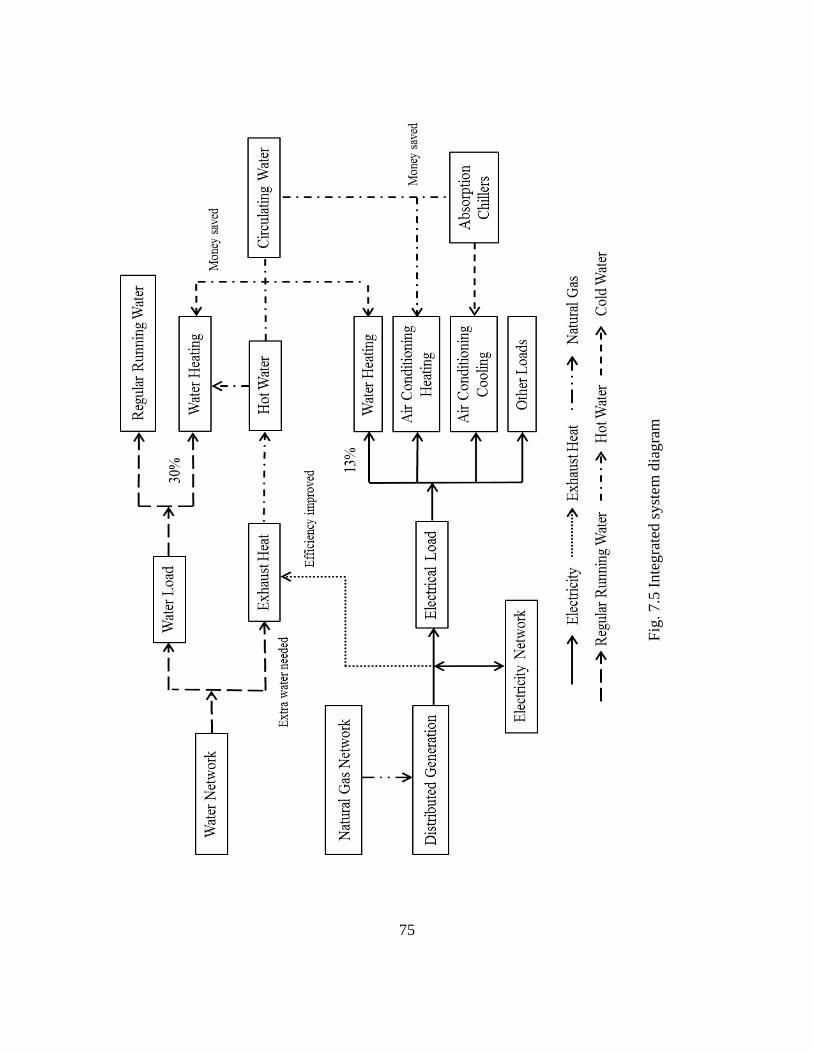
75
Fig
. 7.5
Inte
gra
ted s
yst
em d
iagra
m

76
7.1 Integrated System Analysis
The integrated system diagram is shown in Fig. 7.5, from which the relationships
between different components of systems are clearly presented.
The electricity is provided by both DERs and the grids to supply the electrical
load, which includes water heating, air conditioning for heating, air conditioning for cool-
ing and the other loads. The natural gas network provides the fuel to power the operation
of the gas-fired DERs. Besides the electricity used to supply the load, all the additional
electricity generated by DERs is sent back to the grids.
The water network is usually used to supply the water load by providing regular
daily consumption water (running water) as well as hot water, which accounts for 30% of
total water usage and could be used for shower, washing, heating and other purposes. Ex-
tra water is needed to take away the exhaust heat from DERs. This amount of extra water
also depends on the air conditioning load, including both heating and cooling purposes.
Money and electricity are thus saved by otherwise buying electricity to supply cooling or
heating load, which improves energy efficiency of the whole system and simultaneously
lessens environmental problems caused by greenhouse gases.
The water carrying the exhaust heat may only partially or fully meet the actual air
conditioning load. The grids together with the DERs provide energy to both electrical
loads and thermal loads. The air conditioning loads vary in different seasons. More extra
water is needed for air conditioning of heating in winter times, and for air conditioning of
cooling in summer times. The extra water from water networks used for air conditioning

77
is actually circulating water and water tank is needed to balance the water supply and
demand. This amount of extra water is periodically released and renewed.
Absorption chillers driven by hot water should be studied, which will replace dis-
persed air conditioners by using centralized air conditioning to improve the whole system
performance as well as economics. Coefficient of Performance (COP) of chillers should
be analyzed to verify economics and efficiency.

78
CHAPTER 8.
RESULTS ANALYSIS AND DISCUSSION OF INTEGRATED SYSTEMS
8.1 Objective
The overall objective of the integrated energy system, as shown in (8.1) is to max-
imize the electrical output and recovered thermal output of the CHP-based DG units. The
electrical output is constrained by the electrical system, gas system and the CHP-based
DG system, while the recovered thermal output is constrained by the electrical system,
water system, gas systme and the CHP-based DG system.
, ,( )FE FT
g n g n
g Gn N
max p p
(8.1)
8.2 Implementation
The integrated system model was coded and implemented in the AIMMS optimi-
zation modeling environment [68], including electrical system model, gas system model,
water system model, and the CHP-based microturbine model. AIMMS is Advanced Inte-
grated Multidimensional Modeling Software, which is excellent for modeling mathemati-
cal programming (MP) problems.
The MP problems are generated by AIMMS from the model structure and data,
for which the first and second derivatives of the constraints may be also generated auto-
matically for nonlinear models when necessary [26]. The generated MP is passed to the
selected efficient commercial solver – the CONOPT 3.14 V generalized reduced gradient
solver.
The integrated system program is actually a non-convex nonlinear MP problem,
and normally there is no guarantee for nonlinear solvers that the global optimum is defi-

79
nitely found. Most often the returned solution is a local optimum or probably no feasible
solution is found. To solve these problems, several possible approaches could be em-
ployed:
Use a global solver, e.g. Baron. Global solvers are usually not efficient and
very time-consuming and only work well on relatively small NLP problems
[68]. The integrated system model also has constraints that include gonio-
metric functions that cannot be handled by Baron.
Use a multistart procedure. This can help provide a better chance to find the
global optimum by tracking and comparing all feasible solutions found. The
multistart algorithm generates multiple random starting points, identifies areas
of points resulting in the same local solution, solves each cluster by using the
selected NLP solver, and then returns the best feasible solution as its final so-
lution [68].
Use a nonlinear presolver. This can help reduce the problem size and tighten
bounds of variables and constraints, with which the research space of finding
one optimum can be reduced by applying reduction techniques [68].
8.3 Integrated System Solving Flowchart
The problem solving flowchart of the integrated system is shown in Fig. 8.1. The
data input of electrical system, water system, gas system, and the CHP-based micro-
turbine system were initialized first. The NLP presolve and multistart procedures were
applied to the electrical system for each phase with the ACOPF formulation. In this way,
the resultant nodal DG output was calculated for each individual phase. The nodal DG

80
power output includes the total nodal DG electrical output and thermal output, which
were achieved by summing up the nodal DG electrical output and thermal output of all
three phases.
According to the nodal DG power output, the corresponding nodal DG gas con-
sumption can be calculated via the power/fuel conversion equation. The total nodal gas
consumption was then updated by adding this DG gas consumption to the existing base
gas load. The total nodal gas consumption was sent to the developed simulation model of
the gas network to check the gas supply capability of the designed gas network. The sim-
ulations were run until no violations occur on the nodal gas pressure limit. If a violation
is found, the nodal DG gas consumption will be reduced accordingly, and the simulation
is rerun until the minimum criterion is reached.
The updated nodal DG power output was determined by the final total nodal gas
consumption. The updated nodal DG power output was then sent to the CHP-based DG
model, where the nodal DG power output functions as the upper bounds of the real nodal
DG electrical output and thermal output. Besides the nodal DG electrical output, the nod-
al DG thermal output is also constrained by the water availability from the water distribu-
tion network and the CHP-based DG system, which are run simultaneously with the input
from the electrical system results. If the minimum nodal water pressure limit is violated,
then less water can be extracted from the water network and thus less thermal energy
would be carried away. This iteration continues until the minimum nodal water pressure
is met. The whole algorithm stops when no violations are found in the water system and
the CHP-based DG system.
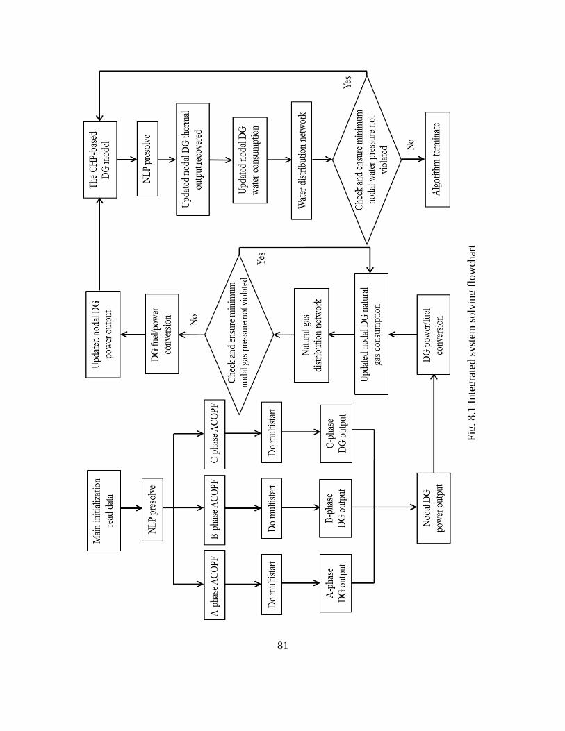
81
Fig
. 8.1
Inte
gra
ted s
yst
em s
olv
ing f
low
char
t
Inte
gra
ted s
yst
em s
olv
ing f
low
char
t

82
8.4 Case Studies
Multiple factors were investigated that primarily affect the electrical output and
recovered thermal output of the CHP-based DG units, such as DG unit capacity, DG
power factor (PF), gas supply, ambient temperature, and nodal water pressure, which will
be explained in detail that how it affects the energy produced. For factors affecting the
DG electrical output, DG unit capacity, DG PF, gas supply and ambient temperature will
be investigated, while for factors affecting DG recovered thermal output, ambient tem-
perature and nodal water pressure will be investigated.
Table 8.1 Electrical System Load
Total Phase Load A-phase Load B-phase Load C-phase Load
Real Power Load (kW) 1420 915 1155
Reactive Power Load (kVAr) 775 515 630
The electrical loading information is shown in Fig. 8.2. As shown in this figure, it
is found that the system loading includes both three-phase load and single-phase load.
Three-phase load is found in nodes 47, 48, 49, 65, and 76, while the single-phase load is
found in some of the rest nodes. Not every node has the electrical load. The system three-
phase real power load and reactive power load are 3490 kW and 1920 kVAr, respectively,
from which the load power factor was calculated to be 0.876. The individual phase load-
ing information is shown in Table 8.1.
8.4.1. Capacity bounds
By changing the capacity of DG units to 65 kW, 130 kW, 325 kW, 650 kW, and 1
MW, five cases from Case 1 to Case 5 were studied to investigate how the change of
units’ capacity affects the DG units’ performance and distribution in the electricity distri-
83
Fig
. 8.2
Ele
ctri
cal
syst
em l
oad
ing s
how
n b
y n
odes
and p
has
es

84
bution network. The DG units were assumed to be placed at every node with a fixed unity
PF. For this analysis, the electrical system was run for optimization while the other sys-
tem models were not integrated and solved together.
The nodal DG electrical output in all five cases is shown in Fig. 8.3. It is found
that not every node is appropriate to place a CHP-based DG unit. In Case 1, since the up-
per bound was set to 65 kW, all nodes are placed with DG units, and about half of them
are operated in triple times of the DG unit capacity. In Case 2, the DG units’ power out-
put increases compared to that in Case 1, while simultaneously the nodes connected with
DG units reduce. In Case 3 and Case 4, the number of nodes with DG units connected
reduces continuously. The reason for this may be that with the increasing upper bound of
unit capacity, a node with DG unit connected continues raising power output until a vio-
lation occurs in that node, if no other constraints are added. In Case 5, the number of
nodes with units connected continues shrinking, and the most nodal electrical output is
found up to 3 MW.
In Case 5, a larger unit size, like 200 kW or 300 kW should be used instead of the
original 65 kW unit considering the economic efficiency. However, a larger size of 1
MW or above is not suggested due to the concern of potential fault level increase. Anoth-
er reason is that a large size of DER in the distribution systems may not sufficiently em-
body the distribution characteristics of DERs, and people in residential communities may
not benefit from this arrangement if the load center is far away from the energy source
and the laying of new thermal pipelines is costly. It is also noted that for nodes with high-
er load, they may be not the same nodes with the most unit electrical output for each case.

85
Fig
. 8.3
CH
P-b
ased
DG
pow
er o
utp
ut

86
For units 95, 119, 121, and 122, which correspond to nodes 95, 197, 300 and 450, they
are all found with the most power output in each case, which are also the nodes with ex-
ternal generators connected. Therefore, it makes more sense that units with the highest
DG capacity are placed in these locations.
The total DG electrical output is shown phase by phase in Fig. 8.4, from which it
is found that both the individual phase DG electrical output and the total DG electrical
output increase steadily with the DG unit capacity increase.
Fig. 8.4 Total DG power output by cases
The real power and the reactive power output of ExGens are shown in Fig. 8.5. It
is known that for all cases, all ExGens actually absorb the real power generated by the
DG units, and provide the reactive power for the DG units. With the unity capacity in-

87
crease, the amount of total real power and reactive power output also grows gradually.
For all cases, the ExGen1 absorbs the least real power from the DG units, while outputs
the most reactive power to the DG units.
The electrical output summary for this study is shown in Table 8.2. The total DG
electrical output rises with the unit capacity increase. It is found that the real power sent
back to the grids is at least 4.82 times of the base electrical load of 3.49 MW in Case 1.
The base natural gas load for the designed gas network is 31.089 mcfh. The total DG gas
consumption is found at least 5.91 times of the base gas load in Case 1.
Fig. 8.5 Real power absorbed and reactive power provided by ExGens by cases

88
The DG penetration level refers to the ratio between the number of nodes with
DG units and the total number of nodes. From Table 8.2, it is shown that not every node
is appropriate to place a DG unit and the penetration level reduces with the unit capacity
increase. However, the penetration level should not be too high or too low. If the penetra-
tion level is too high, for example, in Case 1, where each node is placed a DG unit, then
the potential fault level and stability issues in this distribution system grow significantly
when all these units work together. If the penetration level is too low, such as in Case 5 or
even lower in other unstudied cases, the economic benefits may not be sufficiently mate-
rialized, e.g., the paving of new thermal pipelines is costly when the load center is located
far away from the thermal supply source.
Table 8.2 Electrical Output Summary
Case Studies Case 1 Case 2 Case 3 Case 4 Case 5
DG Power Output (MW) 16.84 23.09 25.22 28.49 32.02
DG Penetration Level (%) 100 89. 3 75.4 62.3 59
Grids Power Output (MW) -13.35 -19.6 -21.73 -25 -28.53
DG Power Supply Ratio 4.82 6.62 7.23 8.16 9.17
DG Gas Usage (mcfh) 183.82 245.70 265.36 296.73 331.98
DG Gas Use Ratio 5.91 7.90 8.54 9.54 10.68
Therefore, in the following sections, Case 3 will be used to as a reference to in-
vestigate other factors’ influences on the electrical output and recovered thermal output
of the CHP-based DG units.
8.4.2. Power factor
Three different DG PFs were studied: 0.95 lag, unity, and 0.95 lead. Similarly,
only the electrical system model was optimized while the other system models were not
integrated and solved.

89
As shown in Fig. 8.6, the overall trend of total DG electrical output is growing
with the unit capacity increase in all cases. For each case, DG outputs the most power at
the unity PF and outputs the least power at the 0.95 PF lag. For Case 3, the most DG
power output is 25.22 MW, which exceeds that at a 0.95 PF lag, and that at a 0.95 lead by
2.13 MW, and 0.72 MW, respectively.
Fig. 8.6 DG unit maximum power output by various power factors
The curves of the DG penetration level with changing PFs are shown in Fig. 8.7.
It is found that for all PFs, the overall trend of the DG penetration level goes down with
the DG unit capacity increase. For the unity PF, the DG penetration level reduces contin-
uously. For the 0.95 PF lead, the DG penetration level reduces as well for all cases. How-
ever, the decreasing trend of the DG penetration level slows down when the unit capacity
is beyond 325 kW. While for the 0.95 PF lag, the DG penetration level reduces the most
down to 33% and remains almost level when the unit capacity is beyond 650 kW.

90
Fig. 8.7 DG penetration level with changing PFs in all cases
Fig. 8.8 The power output of ExGens for various power factors
For PFs of 0.95 lag and unity, the reactive power is supplied by the electrical sys-
tem and all shunt capacitors working in full capacities. When the PF is 0.95 lead, the

91
electrical system absorbs all extra DG reactive power output. The PF of most DG units
can be specified according to customer requirements.
In Fig. 8.8, the real and the reactive power output of ExGens are shown consider-
ing various units power factors. All of these ExGens are actually absorbing the extra real
power delivered by the DG units, in which the most real power is sent to ExGen2, while
ExGen1 absorbs the least real power. Similarly, for each ExGen, the maximum power
absorbed always appears at a unity power factor. All ExGens send reactive power to the
system at power factors of 0.95 lag and unity, in which ExGen2 sends the most. When
the power factor is 0.95 lead, all ExGens absorb the extra reactive power from the system.
8.4.3. Gas supply
The DG penetration adds up additional gas demand to the present gas system. The
total nodal gas demand was used as the input to run the static gas flow simulation. For
this case study, only the water system was not integrated while all the other systems were
solved and analyzed together. First, all five cases at a unity PF were optimized and the
individual gas consumption was checked in the designed gas system. Then the larger di-
ameter of gas mains was changed from originally 6 inches into 4 inches and 2 inches to
investigate the gas supply capability with the large DG penetration. The total nodal gas
consumption in all five cases is shown in Fig. 8.9. Since this total nodal gas consumption
includes the existing nodal base load, the distribution profile of the nodal gas consump-
tion is a little different from the corresponding distribution profile of the nodal DG elec-
trical output. However, in general, these two distribution profiles are consistent.

92
Fig
. 8.9
Tota
l nodal
gas
consu
mpti
on
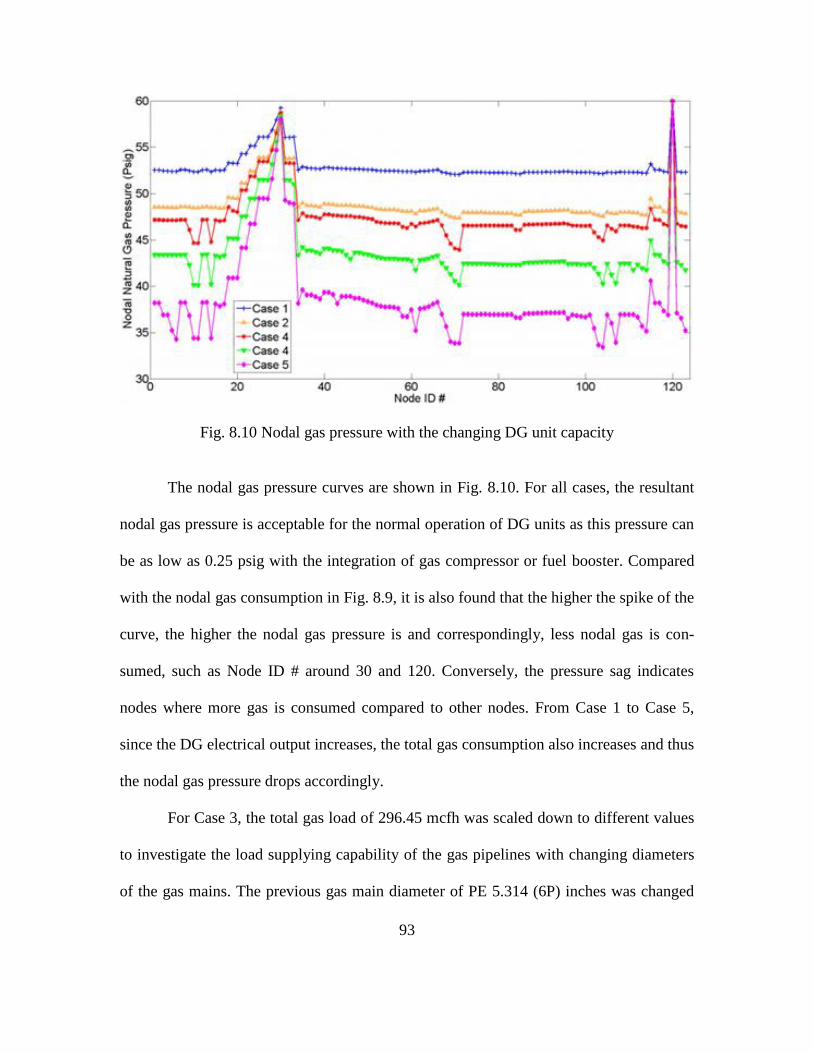
93
Fig. 8.10 Nodal gas pressure with the changing DG unit capacity
The nodal gas pressure curves are shown in Fig. 8.10. For all cases, the resultant
nodal gas pressure is acceptable for the normal operation of DG units as this pressure can
be as low as 0.25 psig with the integration of gas compressor or fuel booster. Compared
with the nodal gas consumption in Fig. 8.9, it is also found that the higher the spike of the
curve, the higher the nodal gas pressure is and correspondingly, less nodal gas is con-
sumed, such as Node ID # around 30 and 120. Conversely, the pressure sag indicates
nodes where more gas is consumed compared to other nodes. From Case 1 to Case 5,
since the DG electrical output increases, the total gas consumption also increases and thus
the nodal gas pressure drops accordingly.
For Case 3, the total gas load of 296.45 mcfh was scaled down to different values
to investigate the load supplying capability of the gas pipelines with changing diameters
of the gas mains. The previous gas main diameter of PE 5.314 (6P) inches was changed

94
to PE 3.621 (4P) inches and PE 1.885 (2P) inches, respectively. The results are shown in
Table 8.3, where the influences of gas main diameter on gas supply and DG electrical
output is presented.
For both 4P and 2P cases, the ratio of nodes with positive gas pressure reduces up
to 78% with a small increase (up to 6.25%) in the scaled total gas load. Nodes with nega-
tive gas pressure cannot supply gas such that the total supplied gas load decreases with
the increase of negative gas pressure nodes. In either case, the base gas load has the prior-
ity of being first supplied, which further reduces the left gas for DG usage. For the 4P
case, the maximum DG power output is 15.17 MW compared to 25.22 MW in the 6P
case; while for the 2P case, the maximum DG power output is only 0.17 MW, about 0.67%
of that in the 6P case. The whole gas network in this case doesn’t work and cannot sup-
port the DG penetration. Therefore, a larger diameter of the gas main increases the line
pack capability and compensates for fluctuations for the natural gas.
Table 8.3 Gas System Performances for Different Gas Mains
Gas Main Size/Type 4P
Scaled Total Gas Load (mcfh) 184.76 187.65 190.53 193.42 196.31
Nodes with Positive Gas Pressure (%) 100 95.9 50.4 29.3 22.0
Gas Load Supplied (mcfh) 184.76 175.55 80.63 46.68 34.88
DG Gas Usage (mcfh) 153.67 144.47 49.54 15.59 3.79
DG Power Output (MW) 15.17 14.26 4.88 1.53 0.36
Gas Main Size/Type 2P
Scaled Total Gas Load (mcfh) 32.91 33.20 33.49 33.78 34.06
Nodes with Positive Gas Pressure (%) 100 67.5 48.8 44.7 27.6
Gas Load Supplied (mcfh) 32.91 20.32 12.52 10.52 8.16
DG Gas Usage (mcfh) 1.82 0 0 0 0
DG Power Output (MW) 0.17 0 0 0 0

95
8.4.4. Ambient temperature
From the above analysis and discussion, the unit capacity was set to 0.325 MW,
and the unity PF was selected to maximize the DG units’ power output and begin the re-
search on the recovered thermal output of DG units. The nodal water pressure was set to
40 m, which is taken as an intermediate value between the acceptable water pressure of
36 m, and the required water pressure of 42 m. A range of different ambient temperatures
AT from 0 to 122 are selected and used as references to study their influences on the
performances of CHP-based DG units. For this case analysis, all system models were in-
tegrated together and analyzed.
Fig. 8.11 DG output with changing ambient temperatures
The total DG electrical output, recovered thermal output and total power output
curves are shown in Fig. 8.11. It is found that ambient temperatures significantly affect
the total DG power output. When AT is below 70 , the electrical output remains un-
changed, while the recovered thermal output decreases with the reduction of AT . When

96
AT is above 70 , the electrical output and the recovered thermal output decreases 5.78%
and 1.39%, respectively for every 10 increase. The total power output reaches the max-
imum 37.24 MW at the AT of 70 , including the recovered thermal output of 12 MW
and the electrical output of 25.2 MW. An indoor environment with an adjustable tem-
perature is suggested to ensure that the units are operated most efficiently.
Fig. 8.12 Nodal DG output with corresponding gas and water consumption
The nodal DG output and corresponding gas and water consumption are shown in
Fig. 8.12 at the AT of 70 . It is found that for the node with DG electrical output, the
thermal output may not be recovered due to the nodal water pressure, water temperature,
and DG water consumption requirements. For Node ID # in the range of 60 to 120, the
majority of nodes are in low water pressures zones, as they are located at the far right side

97
of the pump. The water head automatically drops with distance increase from the pump if
no other pumps are present in the distribution network For DG water usage, the higher
the nodal water head limit is, the less the extra water available for recovering exhaust
heat. If additional pumps are added to the right side of the water network, the water head
will rise and more exhaust heat in these nodes will recovered.
8.4.5. Nodal water pressure
The nodal water pressure is a main factor determining and constraining the water
consumption of CHP-based DG units and thus the recovered thermal output. The required
water head was set to 42.2 m and the acceptable water head was set to 35.2 m in this
study. A water head above 35.2 m is acceptable and several water heads, 36 m, 38 m, 40
m, and 42 m, were selected for comparison purposes. In addition, the DG unit capacity
was set to 0.325 MW at a unity PF and AT of 70 to maximize the DG output.
Fig. 8.13 DG output with different nodal water heads

98
The total electrical output and recovered thermal output of the CHP-based DG
units are shown in Fig. 8.13. It is found that for all nodal water heads, the electrical out-
put remains unchanged, while the recovered thermal output decreases significantly with
the increase of the nodal water head limit, from 23.7 MW at 36 m to 4.21 MW at 42 m.
Since the water used to recover the exhaust heat is the additional water extracted from the
existing water distribution system, it adds burden to the total water supply. The use of
this additional water should not influence or interrupt the normal consumption and distri-
bution of the existing water supply. By considering other factors, such as the required
thermal storage size, economic benefits, thermal balance between demand and supply,
investment and income, it is advisable to set the nodal water head no lower than 38 m.
Fig. 8.14 Nodal water head with different limits requirements

99
The nodal water head curves with different limit requirements are shown in Fig.
8.14. The top black line indicates the nodal water head with existing water demand, while
all remaining curves represent the nodal water heads with extra water used by the CHP-
based DG units under different water head limits. For Node ID # between 20 and 70, the
nodal water heads are higher than all remaining nodes with the exception of nodes clus-
tered around 120, which are located close to the pump. While for Node ID # between 60
and 120, they correspond to the nodes with lower water pressures, as they are located at
the far right side of the pump in the water distribution network. The water head decreases
automatically with the increasing distance from the pump.
Fig. 8.15 DG water use with different nodal water heads
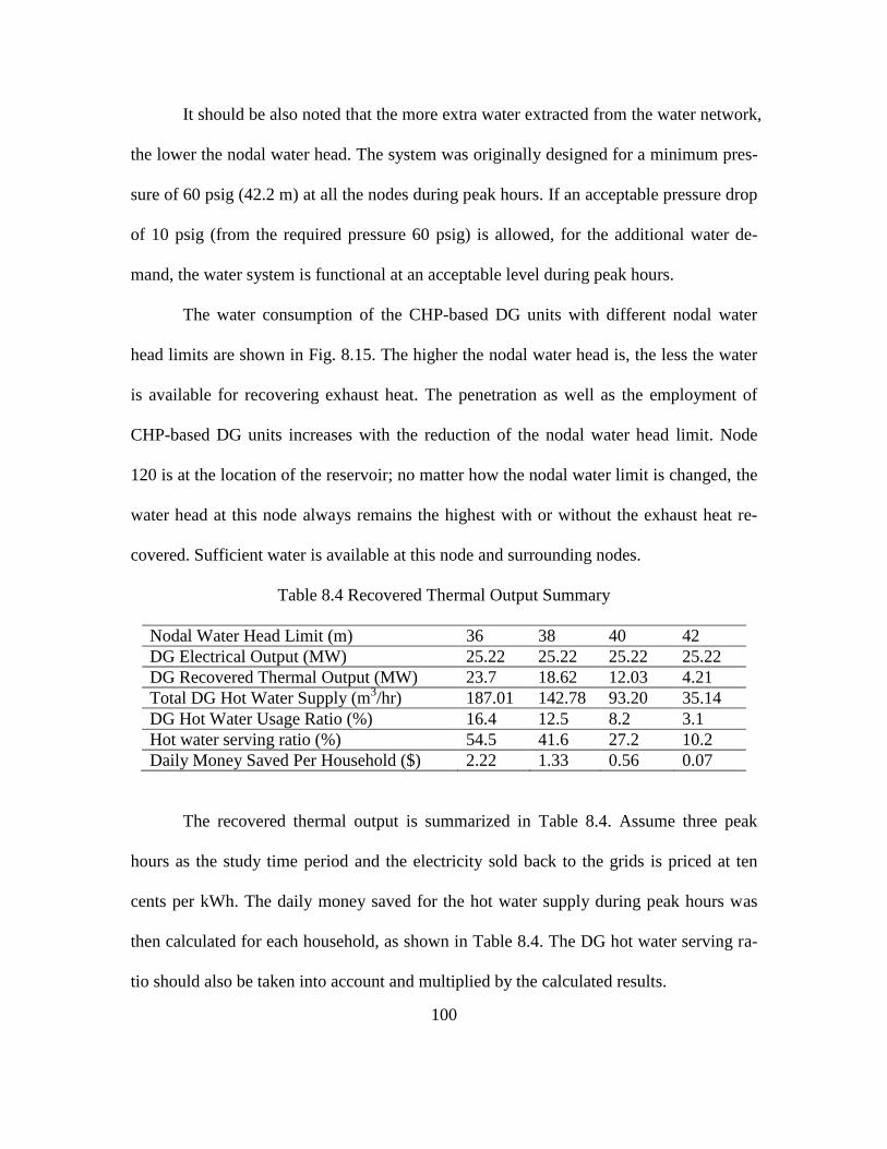
100
It should be also noted that the more extra water extracted from the water network,
the lower the nodal water head. The system was originally designed for a minimum pres-
sure of 60 psig (42.2 m) at all the nodes during peak hours. If an acceptable pressure drop
of 10 psig (from the required pressure 60 psig) is allowed, for the additional water de-
mand, the water system is functional at an acceptable level during peak hours.
The water consumption of the CHP-based DG units with different nodal water
head limits are shown in Fig. 8.15. The higher the nodal water head is, the less the water
is available for recovering exhaust heat. The penetration as well as the employment of
CHP-based DG units increases with the reduction of the nodal water head limit. Node
120 is at the location of the reservoir; no matter how the nodal water limit is changed, the
water head at this node always remains the highest with or without the exhaust heat re-
covered. Sufficient water is available at this node and surrounding nodes.
Table 8.4 Recovered Thermal Output Summary
Nodal Water Head Limit (m) 36 38 40 42
DG Electrical Output (MW) 25.22 25.22 25.22 25.22
DG Recovered Thermal Output (MW) 23.7 18.62 12.03 4.21
Total DG Hot Water Supply (m3/hr) 187.01 142.78 93.20 35.14
DG Hot Water Usage Ratio (%) 16.4 12.5 8.2 3.1
Hot water serving ratio (%) 54.5 41.6 27.2 10.2
Daily Money Saved Per Household ($) 2.22 1.33 0.56 0.07
The recovered thermal output is summarized in Table 8.4. Assume three peak
hours as the study time period and the electricity sold back to the grids is priced at ten
cents per kWh. The daily money saved for the hot water supply during peak hours was
then calculated for each household, as shown in Table 8.4. The DG hot water serving ra-
tio should also be taken into account and multiplied by the calculated results.

101
It is known that the total base hot water load is 342.97 m3/hr, and the total base
water load is 1143.24 m3/hr. The hot water usage ratio compared to the total base water
load is calculated and the results indicate that the hot water supply is only partially met
from 10.2% to 54.5%. Therefore, the money saved is prorated and shown in Table 8.4.
Savings accrue by directly using the hot water supplied by the DG units, which would
otherwise have been bought from the grids.
8.5 Results Analysis and Discussion
The integrated system model was solved as a non-convex nonlinear optimization
problem. A local found solution may not necessarily represent the global optimum. It
should be noted that for any large nonlinear non-convex planning problems, finding a
global solution is impractical and not guaranteed. Since at present there is no efficient
global solution available for this specific problem, the algorithms of nonlinear presolve
and multistart were employed to find the best optimum by comparing all found local op-
tima. This method has been employed and only a local solution was found, which proved
to generate by far the best results achieved for this specific planning application and like-
ly to be the global results. For this specific planning problem, a technique with an achiev-
able solution provides more value than a global optimum which cannot be guaranteed for
other cases [26]. In should be noted that in a distribution system without many meshed
loops, such as that shown in Fig. 4.2, it is highly possible that a single local optimum ex-
ists.
It is found that that for all the cases studied, the CHP application cannot be em-
ployed at every node. Therefore, for nodes where there are no units connected, other

102
heating equipment is supposed to be available, such as boilers. For each nodal water head
limit, it is highly possible that not all units’ exhaust heat can be recovered to supply the
thermal demand. The reason for this may be that for each case, the minimum hourly nod-
al thermal supply of units may be much more than the hourly thermal demand. This also
means that during the peak three hours, units providing the thermal supply may only need
to be operated less than the full three-hour period. At that point, they stop providing
thermal supply unless other purposes of additional thermal use are suggested, such as air
conditioning by using absorption chillers, where the hot water is used as the thermal me-
dium to produce cold or chilled water. Normally, a hot water tank is used as storage to
temporarily store the hot water and provide balance between thermal supply and thermal
demand. The boiler may be used to provide the additional thermal supply when there is a
deficiency.
It has been demonstrated that for all the cases studied, only a part of the exhaust
heat is recovered and the existing water distribution system cannot support completely
the recovery of exhaust heat. However, for the existing gas network, it functions well and
can provide enough gas to supply the DG penetration. The integrated system performance
depends on a couple of actors. For the DG unity capacity, however, in real employment,
other concerns such as safety issues, system stability, fault level increase, investment and
income, location availability, should also be taken into account. In real deployment, the
PF for most DG units is actually pre-fixed and can be customized according to the cus-
tomers’ requirements. The ambient temperature influences significantly total DG output.
A special indoor or outdoor environment is thus suggested to provide to an adjustable

103
temperature, which ensures the DG units are always operated in the best conditions. The
size of the gas main diameter limits the line pack capability significantly. A small in-
crease of the gas demand may result in a great reduction on the nodal gas pressure. The
nodal water head limit mainly influences the thermal heat recovered. The determination
of water head limit during the planning period must consider present water demand, fu-
ture demand growth and potential thermal applications.

104
CHAPTER 9.
CONCLUSIONS AND FUTURE WORK
9.1 Conclusions
The developed integrated system model offers one generalized means of deter-
mining the maximum DG network capacity accommodated based on urban energy net-
works, from which DG siting and sizing are determined for given electricity, gas and wa-
ter network configurations and the gas-fired DG unit model, as well as the loading infor-
mation.
The overall objective of the integrated system is to maximize the electrical output
and recovered thermal output of the CHP-based DG units. This is different from cost
minimization problems as more congestion may appear not only in the electricity network,
but also in the water network or gas network. The proposed approach is generalized and
can be used not only in the meshed network but also in a radial distribution system, as
shown in [25]. For this application, the generalized integrated system model is especially
innovative and valuable.
The study conducted in this dissertation mainly solves the problem of the network
capacity assessment of the CHP-based DG on urban energy distribution networks, by de-
termining the optimal DG siting and sizing, as well as by quantifying the mutual impacts
between the CHP-based DG units and the urban energy networks. For this reason, the
electrical system model was first developed and modified properly. The corresponding
water and gas distribution systems were then developed to be integrated with the electri-
cal system via the coupling of the CHP-based DG system model. These four system

105
models were developed individually and integrated together to constrain the units’ elec-
trical output and recovered thermal output. The nodal water pressure and the gas main
diameter were checked to identify whether the existing water and gas distribution net-
works could support the large penetration of the CHP-based DG units to increase the sys-
tem energy efficiency. The units’ electrical output and recovered thermal output were
both treated as continuous decision variables, and the units are placed to every node in
the integrated system rather than being fixed into certain nodes. The nonlinear presolve
and multistart algorithms were employed to find a better result by comparing all found
local optima.
The conducted research work for the residential area lays solid foundation for the
later work of the network DG capacity assessment based on urban energy infrastructures.
The selections and model buildings of DERs, electrical load and thermal load, results
analysis and discussion, and the feasibility investigation towards water and natural gas
availability in the residential community contribute to and expand the later research work
focusing on the DG capacity in larger and more complicated systems.
It has been demonstrated that for all the cases studied, the electrical system is ca-
pable of incorporating the large penetration of DERs at the distribution level. This is
changing the way the traditional electricity is generated and transported based on substa-
tions and long-distance high voltage transmission lines. The designed water distribution
system cannot support the complete recovery of exhaust heat, which means in this situa-
tion most waste heat is still emitted into the air. However, wherever there is exhaust heat
recovered, the whole system’s energy efficiency will be improved. For the designed natu-

106
ral gas network, it functions well and can support the large penetration of the gas-fired
DERs. However, the gas main diameters constrain the line pack capability significantly
even if the nodal pressure limit is satisfied. The economic and environmental benefits
brought by the introduction of large DG penetration into the distribution system are in-
creasing the overall social welfare.
9.2 Contributions
An innovative study on the DG planning based on urban energy infrastructures
has been conducted. As a result, the following contributions have been made based on the
conducted research work:
Feasibility investigation for the employment of DERs in urban areas
A real test bed in a residential community was selected and used as the study ob-
ject. Based on this test bed, a novel residential microgrid design method was developed.
The residential energy infrastructures, including water and natural gas infrastructures
were also investigated to identify if they can support the normal operation of the selected
DERs.
An innovative generalized model was developed to assess the DG network ca-
pacity based on urban energy infrastructures
The urban energy infrastructure models, including electrical system, natural gas
and water networks, were developed and integrated by the coupling of CHP-based DG
system model. This is novel as this is the first instance of the CHP-based DG network
capacity assessment by considering the water and gas distribution networks.

107
DG units are placed at every node, rather than being fixed into some nodes in the
integrated system, and function as continuous decision variables
This solution approach is completely new and first employed in the network ca-
pacity assessment of the CHP-based DG units based on urban energy infrastructures. The
generalized solution approach can also be applied in other urban areas or at the transmis-
sion level.
The objective is to maximize the DG units’ output
The difference between this objective and other similar objectives is that the DG
units’ output includes two parts, the electrical output and the recovered thermal heat, both
of which are constrained by different systems. This is also new.
Non-convex nonlinear problem solving
The integrated system model is a non-convex nonlinear problem, which is also a
large system planning problem. The nonlinear presolve and multistart algorithms were
employed to find the best results.
Public welfare accumulates
Money and electricity are saved and environmental problems caused by green-
house gases are also lessened by employing the CHP-based DG units with proper plan-
ning.
9.3 Future Work
The conducted research work mainly focuses on the feasibility investigation of
employing DG technologies in the urban areas and the network capacity assessment of
DG based on urban energy networks by developing and integrating together the electrical

108
system model, gas system model, water system model, and the CHP-based DG system
model.
In the future, work will be conducted in the following aspects:
Develop the mathematical model of the natural gas network
The mathematical model of the natural gas distribution system will be developed
and integrated with the electrical system. The problem of this integration is that for the
integrated system model, it is very difficult to solve or not solvable by available commer-
cial solvers due to the size of the problem and the complexity of the integrated whole sys-
tems, including the electrical system, water and gas systems, and the CHP-based DG sys-
tem.
Thermal load modeling including absorption chillers
For this study, the recovered thermal output was not analyzed sufficiently for its
utilization. The relationship between the hot water supplied to absorption chillers and the
cold/chilled water or hot water output needs to be identified and further quantified.

109
REFERENCES
[1] D. J. Cox, “Microgrid infrastructure modeling for residential Microgrids,” IEEE
Power Engineering Society General Meeting, pp. 1-6, 24-28 June 2007.
[2] R. H. Lasseter, “Certs microgrid,” IEEE System of Systems Engineering, pp. 1-5,
April 2007.
[3] European Research Project “Microgrids”. [Online]. Available: http://www.microgr
ids.eu/index.php?page=kythnos&id=2
[4] Perfect Power at IIT. [Online]. Available: http://www.iit.edu/perfect_power/
[5] S. Kusagawa, E. Masada, J. Baba, M. Ohshima, I. Nagy, “Coordinate control of
distributed generations with power converters in a micro grid,” European Confer-
ence on Power Electronics and Applications, pp. 10, 2005.
[6] K. Nishikawa, J. Baba, E. Shimoda, T. Kikuchi, Yu Itoh, T. Nitta, S. Numata, E.
Masada “Design methods and integrated control for microgrid,” IEEE Power and
Energy Society General Meeting, pp. 1-7, 2008.
[7] P. Piagi, R. H. Lasseter, “Autonomous control of microgrids,” IEEE Power Engi-
neering Society General Meeting, 16 October 2006.
[8] R. Esmaili, D. Das, D. A. Klapp, O. Dernici, D. K. Nichols, “A novel power con-
version system for distributed energy resources,” IEEE Proceedings of Power En-
gineering Society General Meeting, pp. 1-6, June 2006.
[9] M. Ilic, F. Galianca, L. Fink, “Power Systems Restructuring, Engineering and
Economics,” Chapter 12, 1998.

110
[10] A. Cano, F. Jurado and J. Carpio, “Influence of micro-turbines on distribution
networks stability,” IEEE Power Engineering Society General Meeting, vol.4, pp.
2158, 13-17 July 2003.
[11] M. A. Laughton, “Fuel cells”, Engineering Science and Education Journal, vol. 11,
no.1, pp 7-16, Feb. 2002.
[12] B. Cook, “Introduction to fuel cells and hydrogen technology,” Engineering Sci-
ence and Education Journal, vol. 11, no. 6, pp. 205-216, Dec. 2002.
[13] R. Chedid, H. Akiki, S. A. Rahman, “A decision support technique for the design
of hybrid solar-wind power systems,” IEEE Transactions on Energy Conversion,
vol. 13, no. 1 , pp. 76-83, March 1998.
[14] C. L. Smallwood, “Distributed generation in autonomous and nonautonomous mi-
crogrids,” IEEE Rural Electric Power Conference, pp. D1-D1_6, 5-7 May 2002.
[15] Distributed Generation. [Online]. Available: http://www.solarbuzz.com/Distribute
dGeneration.htm
[16] S. R. Guda, C. Wang, M. H. Nehrir, “A simulink-based microturbine model for
distributed generation studies”, 37th Annual North American Power Symposium,
pp. 269-274, 23-25, October 2005.
[17] H. Aki, “The penetration of micro CHP in residential dwellings in Japan,” Power
Engineering Society General Meeting, 24-28 June 2007, pp. 1-4.
[18] Microturbines. [Online]. Available: http://www.energy.ca.gov/distgen/equipment/
microturbines/microturbines.html
[19] Methods for calculating efficiency, [Online]. Available: http://www.epa.gov/chp/b
asic/methods.html.

111
[20] A. D. Hawkes, P. Aguiab, B. Croxford, M. A. Leach, C. S. Adjiman, and N. P.
Brandon, “Solid oxide fuel cell micro combined heat and power system operating
strategy: Options for provision of residential space and water heating,” J. Power
Sources, vol. 164, no. 1, Jan. 2007.
[21] R. U. Ayres, H. Turton, and T. Casten, “Energy efficiency, sustainability and eco-
nomic growth,” Energy, vol. 32, no. 5, May 2007.
[22] W. Graus and E. Worrell, “Trend in efficiency and capacity of fossil power gener-
ation in the EU,” Energy Policy, vol. 37, no. 6, Jun. 2009.
[23] M. Chaudry, J. Ekanayake, and N. Jenkins, “Optimum control strategy for a CHP
unit,” International Journal of Distributed Energy Resources, vol. 4, no. 4, pp.
265-280, 2008.
[24] X. Zhang, G. Karady and Y. Guan, “Design methods investigation for residential
microgrid infrastructure,” Euro. Trans. Electr. Power, vol. 21, pp. 2125-2141,
2011.
[25] X. Zhang, G. Karady, K. Piratla, and S. Ariaratnam, “Nexus between distributed
generation and urban water infrastructure,” IEEE Power Eng. Soc. General Meet-
ing, pp. 1-8, 2012.
[26] C. J. Dent, L. F. Ochoa, and G. P. Harrison, “Network distributed generation ca-
pacity analysis using opf with voltage step constraints,” IEEE Trans. Power Syst.,
vol. 25, no. 1, pp. 296-304, 2010.
[27] C. J. Dent, L. F. Ochoa, G. P. Harrison, and J. W. Bialek, “Efficient secure ac opf
for network generation capacity assessment,” IEEE Trans. Power Syst., vol. 25, no.
1, pp. 575-583, 2010.
[28] G. Celli, E. Ghiani, S. Mocci, and F. Pilo, “A multiobjective evolutionary algo-
rithm for the sizing and siting of distributed generation,” IEEE Trans. Power Syst.,
vol. 20, no.2, pp. 750-757, 2005.

112
[29] X. Zhang, R. Sharma, and Y. He, “Optimal energy management of a rural mi-
crogrid system using multi-objective optimization,” IEEE PES Innovative Smart
Grid Technologies Conference, pp. 1-8, 2012.
[30] W. EI-Khattam, Y. Hegazy, and M. Salama, “An integrated distributed generation
optimization model for distribution system planning,” IEEE Trans. Power Syst.,
vol. 20, no.2, pp. 1158-1165, 2005.
[31] A. Piccolo, and P. Siano, “Evaluating the impact of network investment deferral
on distributed generation expansion,” IEEE Trans. Power Syst., vol. 24, no. 3, pp.
1559-1567, 2009.
[32] W. EI-Khattam, K. Bhattacharya, Y. Hegazy, and M. Salama, “Optimal invest-
ment planning for distributed generation in a competitive electricity market,” IEEE
Trans. Power Syst., vol. 19, no. 3, pp. 1674-1684, 2004.
[33] C. Wang and M. H. Nehrir, “Analytical approaches for optimal placement of dis-
tributed generation sources in power system,” IEEE Trans. Power Syst., vol. 19,
no. 4, pp. 2068-2076, Nov. 2004.
[34] N. Acharya, P. Mahat, and N. Mithulananthan, “An analytical approach for dg al-
location in primary distribution network,” Int. J. Elect. Power Energy Syst., vol. 28,
no. 10, pp. 669-678, Dec. 2006.
[35] M. Geidl, and G. Andersson, “Optimal power flow of multiple energy carriers,”
IEEE Trans. Power Syst., vol. 22, no. 1, pp. 145-155, Feb. 2007.
[36] M. Arnold, R. R. Negenborn, G. Andersson, and B. De Schutter, “Model-based
predictive control applied to multi-carrier energy systems,” IEEE Power Eng. Soc.
General Meeting, pp. 1-8, 2009.
[37] C. Unsihuay-Vila, J. Marangon-Lima, A. de Souza, I. Perez-Arriaga, and P. Ba-
lestrassi, “A model to long-term, multiarea, multistage, and integrated expansion
planning of electricity and natural gas systems,” IEEE Trans. Power Syst., vol. 25,
no. 2, pp. 1154-1168, 2010.

113
[38] A. Martinez-Mares, C. Fuerte-Esquivel, “A unified gas and power flow analysis in
natural gas and electricity coupled networks,” IEEE Trans. Power Syst., vol. 27,
no. 4, pp. 2156-2166, 2012.
[39] C. Unsihuay, J. Lima, and A. de Souza, “Modeling the integrated natural gas and
electricity optimal power flow,” IEEE Power Eng. Soc. General Meeting, pp. 1-7,
2007.
[40] B. Awad, M. Chaudry, J. Wu, and N. Jenkins, “Integrated optimal power flow for
electric power and heat in a microgrid,” 20th
International Conference and Exhibi-
tion on Electricity Distribution, pp. 1-4, 2009.
[41] E. M. Gil, “Modeling integrated energy transportation networks for analysis of
economic efficiency and network interdependencies,” North Amer. Power Symp.
(NAPS), Rolla, MO, 2003.
[42] B. Bakken and A. T. Holen, “Energy service systems: Integrated planning case
studies,” IEEE Power Eng. Soc. General Meeting, Denver, CO, 2004.
[43] T. Lambert, P. Gilman, P. Lilienthal, Micropower system modeling with HOMER,
Integration of Alternative Sources of Energy, December 2005.
[44] SRP, Residential Rates Information, the Basic Plan. [Online]. Available:
http://www.srpnet.com/prices/pdfx/BasicPlan1009.pdf
[45] Egrid 2007 Version 1.1 Year 2005 Summary Tables, December 2008
[46] Renewable Energy Design Guide & Catalog, 2008-2009
[47] National Renewable Energy Lab, PVWATTS, version1. [Online]. Available:
http://rredc.nrel.gov/solar/calculators/PVWATTS/version1/
[48] SRP incentives for residential PV installation. [Online]. Available:
http://www.srpnet.com/environment/earthwise/solar/default.aspx

114
[49] Capstone Turbine Corporation. Technical reference. Application Guide – Model
C65 Integrated CHP (ICHP), CA 91311, USA.
[50] L. Goldstein, B. Hedman, D. Knowles, S.. Freedman, R. Woods, T. Schweizer,
"Gas-fired distributed energy resource technology characterizations," National Re-
newable Energy Laboratory, NREL/TP-620-34783, November 2003.
[51] GenSys Blue fuel cell. [Online]. Available: www.plugpower.com
[52] VRB battery. [Online]. Available: http://www.pdenergy.com/
[53] Power Partners Inc. [Online]. Available: http://www.eco-maxchillers.com/
[54] Water distribution pipe. [Online]. Available: http://www.engineeringtoolbox.com/
water-distribution-pipe-d_1103.html
[55] C. L. Cooper, G. G. Karady “Economic feasibility investigation of a 5kW residen-
tial fuel cell system,” IEEE Power Engineering Society General Meeting, June
2005; pp. 2696-2701.
[56] W. H. Kersting, “Radial distribution test feeder,” IEEE Trans. Power Syst., vol 6,
no. 3, pp. 975-985, 1991.
[57] How The System Works, PG&E’s natural gas system.
[58] Bradley B. Bean, PE, GASWorkS. [Online]. Available: http://www.b3pe.com/
[59] Residential consumption of natural gas per capita in Arizona. [Online]. Available:
http://apps1.eere.energy.gov/states/residential.cfm/state=AZ
[60] Gas Age Magazine, May 1967, Gas Behavior in Distribution Systems.

115
[61] GW90_Manual, GASWorkS 9.0, Bradley B. Beann, PE, 1991-1997, 2006, 2007,
2009.
[62] L. J. Murphy, and A. R. Simpson, “Pipe optimization using genetic algorithms,”
Res. Rep., no. R93, 1992.
[63] D. A. Savić, J. Bicik, and M. S. Morley, “A dss generator for multiobjective opti-
misation of spreadsheet-based models,” Environmental Modelling and Software,
vol. 26, no. 5, pp. 551-561, 2011.
[64] L. A. Rossman, EPANET: User’s manual, U.S. EPA, Cincinnati.
[65] L. W. Mays, Water Distribution Systems Handbook, McGraw-Hill.
[66] K. Piratla, “Investigation of sustainable and reliable design alternatives for water
distribution systems,” Ph.D. Dissertation, Del E. Webb School of Construction,
Arizona State University, Tempe, May 2012.
[67] L. W. Mays, Hydraulic Design Handbook, New York: McGraw-Hill, 1999.
[68] J. Bisschop and M. Roelofs, AIMMS-The User’s Guide, Paragon Decision Tech-
nology, 2006.

116
APPENDIX A
SOFTWARE LIST

117
The whole work presented in this dissertation was finished based on a couple of
software. Each of the software was briefly introduced when it was first used in corre-
sponding model development. The full list is shown below:
HOMER
PVWATTS
EXCEL
AIMMS
EPANET
GANetXL
GASWorkS


