Neoclassical Miracles

Rodolfo E. Manuelli and Ananth Seshadri∗

Department of Economics

University of Wisconsin-Madison

October 2009 - Preliminary

Abstract

We study the dynamic behavior of a Neoclassical growth model

with finite lifetimes and imperfect altruism in which individuals can

accumulate both physical and human capital. We use the model to

better understand and explain the behavior of economic miracles. Our

results suggest that standard Neoclassical forces can account for the

performance of the miracle economies and can explain the protracted

transition that is inconsistent with the predictions of a Neoclassical

set-up with only physical capital. The model is also consistent with

the dramatic rise in investments in physical and human capital that

these miracle economies experienced.

∗Seshadri thanks the Alfred P Sloan Foundation for financial support.

1

1 Introduction

In any empirical analysis of cross country economic performance it is easy

to find a few episodes of fast growth, as well as many instances of economic

stagnation. A major challenge for economic theory is to identify what are the

driving forces behind the successes and failures. Ultimately, the objective

of the theory is to come up with a recipe that a country can use to produce

economic miracles. No amount of atheoretical empirical work can discover

the engines of growth. Since there are plenty of theoretical models that can,

on paper, produce economic miracles, it is necessary to better understand

the implications of these models for how an economy responds to shocks, as

a prerequisite to finding the growth silver bullet.

To the extent that alternative theoretical models have different impli-

cations for the evidence, it seems that a reasonable way to evaluate those

models is to quantify their predictions for economic variables that can be

measured. The ability of the simple one sector neoclassical growth model

to account for growth observations –along a transition path– came into

question based on the results of King and Rebelo (1993). Their findings

show that if capital share is of the order that we observe in the data, the

model implies fast convergence and large changes in the marginal product of

capital. On the other hand, if (broadly defined) capital share is large, then

convergence is very slow.

Following Lucas (1993), there has been renewed interest in understand-

ing growth miracles. Lucas, tentatively concluded that human capital –

including schooling and an unmeasured quality dimension– is the key to

understanding episodes of fast growth. At the same time, work by Young

(1995) and others quantified the evolution of several economic variables,

2

investment, years of education in the work force and measures of productiv-

ity, among others, for the fast growing countries of East Asia. The ultimate

goal was to determine the contribution of each factor to the growth miracles.

Since measurement along the lines of Young assumes a particular economic

model, alternative specifications of the economy can render the conclusions

suspect.

One of the major issues in understanding growth miracles is the iden-

tification of the class of models that can be consistent with the observed

miracles. In particular, substantial attention has been given to the possibil-

ity that the standard one sector neoclassical growth model, that has proved

very successful replicating business cycle data, can also account for episodes

of fast growth and stagnation. Prescott and Hayashi (2002) argued that low

TFP growth explains Japan’s poor performance since the early 1990s. More

recently, Chen, Ïmrohoroglu and Ïmrohoroglu (2006) find that the simple

model can also account for the large differences in saving rates between U.S.

and Japan. Other studies, e.g. Chang and Hornstein (2007) and Papa-

georgiu and Perez-Sebastian (2005), suggest that models that deviate from

the standard model are needed to explain the economic performance of East

Asian countries.

In this paper, we revisit the neoclassical growth model. We follow Lucas’

suggestion that human capital has both a quality and a quantity dimension,

and that on-the-job training is an important component of aggregate human

capital. Moreover, we take the mortality of human beings seriously and

restrict the model so that human (but not physical) capital owned by an

individual completely depreciates at death. In order to model human capital

in a way that is consistent with observed age-earnings profiles –which we

view as the prime evidence on the effect of human capital over a lifetime–

3

we use a version of the Ben-Porath (1967) model.

We perform several experiments. First, as in King and Rebelo, we study

the predictions of the model to one time shocks to exogenous variables. We

consider changes in (actual) TFP, fertility and the relative price of capital.

Our major finding is that the model produces adjustment paths that are

quite different from those identified by King and Rebelo, even though our

common parameters are chose to have similar values. In particular, we esti-

mate that the response of investment to a one time shock in TFP is hump

shaped, and not decreasing. Thus, the behavior of the saving rate in some

growing economies could, potentially, be consistent with simple productivity

shocks. We also find that conventionally measured TFP increases by much

more than actual TFP, and the increase is distributed over a much longer

period of time. Of course, the difference between actual and measured pro-

ductivity is driven by changes in the quality of human capital, both due to

changes in the quality of schooling and in the amount of on-the-job training.

Once and for all decreases in fertility (that correspond to a change in

population growth rate from 4% to 2%) have a large impact on output, with

just a small fraction of the ultimate change occurring in the first 10 years.

As in the case of a TFP shock, the reason lies in the behavior of human

capital. A demographic shock ultimately implies a lower effective interest

rate and this induces a higher investment in physical and human capital.

In both of our one shock experiments we find that, after the first period

in the case of a TFP shock, the response of the growth rate of output per

worker is hump shaped: There is a small increase in the 10 years following

the shock, and then another period –approximately lasting 10 years as

well– in which the growth rate increases. Finally, the growth rate settles

into its long run value of 0. We use the model to decompose the growth

4

experience of the “average” of the fast growing economies of the Far East

and we find that demographic change accounts for over 30% of the observed

increase in output per worker, while pure TFP shocks explain approximately

44% of the change. The residual is due to the joint effects.

We also use the model to evaluate how well it reproduces the economic

performance of the Asian Tigers and some Latin American economies. When

we pick TFP to match output per worker and we use observed demographic

data, the model is broadly consistent with the evidence from the East Asian

economies. Even though the fit is far from perfect, the model is able to

reproduce the positive association between investment rates (in physical

capital) and schooling.

Finally, we ask whether opening up the economy can lead to large aggre-

gate changes. We find that it can. Opening up the economy in 1960 would

lead to large aggregate effects and can account for more than 50% of the

change in output per worker between 1960 and 2000.

2 Model

The model uses the same technology as in Manuelli and Seshadri (2007).

We view the economy as being populated by overlapping generations of

individuals who live for T periods. The time line is the following: After

birth, say at time t0, an individual remains attached to his parent until he

is I years old (at time t0 + I); at that point he creates his own family and

has, at age B (i.e. at time t0+B), ef(t0+B) children that, at time t0+B+I,

leave the parent’s home to be become independent.

The utility functional of a parent who has h units of human capital, and

initial wealth (a bequest from his parents) equal to b, at age I, in period t

5

is given by

V P (h, b, t) =

∫ T

I

e−ρ(a−I)u[c(a, t+ a− I)]da+ e−α0+α1f(t+B−I) (1)

∫ I

0e−ρ(a+B−I)u[ck(a, t+B − I + a)]da

+e−α0+α1f(t+B−I)e−ρBV k(hk(I), bk, gk, t+B),

where c(a, t) [ck(a, t)] is consumption of a parent (child) of age a at time t.

The term f(t) denotes the log of the number of children born at time t.

We assume that parents are imperfectly altruistic: The contribution

to the parent’s utility of a unit of utility allocated to an a year old child

attached to him is e−α0+α1f(t+B−I)e−ρ(a+B−I), since at that time the parent

is a+B years old. In this formulation, e−α0+α1f(t+B−I) captures the degree

of altruism. If α0 = 0, and α1 = 1, the preference structure is similar

to that in the infinitively-lived agent model. Positive values of α0, and

values of α1 less than 1 capture the degree of imperfect altruism. The term

V k(hk(I), bk, gk, t + B) stands for the utility of the child at the time he

becomes independent.

Each parent maximizes V P (h, b, t) subject to two types of constraints:

the budget constraint, and the production function for human capital. The

6

former is given by

∫ T

I

e−∫t+a−I

tr(s)dsc(a, t+ a− I)da+ (2)

ef(t+B−I)∫ I

0e−

∫t+a+B−I

tr(s)dsck(a, t+B − I + a)da

+

∫ R

I

e−∫t+a−I

tr(s)dsx(a, t+ a− I)da+

ef(t+B−I)∫ I

0e−

∫t+a+B−I

tr(s)dsxk(a, t+B − I + a)da+

ef(t+B−I)e−∫t+B

tr(s)dsbk + ef(t+B−I)e−

∫t+B+6−I

tr(s)dsxE

≤

∫ R

I

e−∫t+a−I

tr(s)dsw(t+ a− I)h(a, t+ a− I)(1− n(a, t+ a− I))da

+ef(t+B−I)∫ I

6e−

∫t+a+B−I

tr(s)ds[w(t+ a+B − I)

hk(a, t+B − I + a)(1− nk(a, t+B − I + a))]da+ b.

Since we are interested in understanding transition effects, we allow the

interest rate and the wage rate to vary over time.

We adopt Ben-Porath’s (1967) formulation of the human capital produc-

tion technology, augmented with an early childhood period. Specifically, we

assume that (ignoring the temporal dependence to simplify notation)

h(a) = zh[n(a)h(a)]γ1x(a)γ2 − δhh(a), a ∈ [I,R) (3)

hk(a) = zh[nk(a)hk(a)]γ1xk(a)

γ2 − δhhk(a), a ∈ [6, I) (4)

hk(6) = hBxυE, (5)

h(I) given, 0 < γi < 1, γ = γ1 + γ2 < 1,

Even if there is perfect altruism, we assume that when an individual

dies, his human capital dies with him. Thus, the depreciation rate is 100%

at age T.

7

If asset transfers are not constrained, the income maximization and util-

ity maximization problems can be solved independently. In this case, it is

optimal for an individual to maximize the present discounted value of net

income. We assume that each agent retires at age R ≤ T . The maximization

problem for an agent born at time t is

maxh,n,x

∫ R

6e−

∫t+a−6

t+6r(s)dse−r(a−6)[w(t+a−6)h(a)(1−n(a))−x(a)]da−xE (6)

subject to

h(a) = zh[n(a)h(a)]γ1x(a)γ2 − δhh(a), a ∈ [6, R), (7)

and

h(6) = hE = hBxυE (8)

with hB given. Equations (7) and (8) correspond to the standard human

capital accumulation model initially developed by Ben-Porath (1967). This

formulation allows for both market goods, x(a), and a fraction n(a) of the

individual’s human capital, to be inputs in the production of human capital.

Investments in early childhood, which we denote by xE (e.g. medical care,

nutrition and development of learning skills), determine the level of each

individual’s human capital at age 6, h(6), or hE for short.1 This formulation

captures the idea that nutrition and health care are important determinants

of early levels of human capital, and those inputs are, basically, market

goods.2

1 It should be made clear that market goods (x(a) and xE) are produced using the

same technology as the final goods production function. Hence the production function

for human capital is more labor intensive than the final goods technology.2 It is clear that parents’ time is also important. However, given exogenous fertility,

it seems best to ignore this dimension. For a full discussion see Manuelli and Seshadri

(2006b).

8

The solution to the problem is such that n(a) = 1, for a ≤ 6 + s(t).

Thus, we identify s(t) as years of schooling of the cohort born at time t.

In the stationary case, i.e. r(s) = r and w(s) = w, Manuelli and Seshadri

(2006)) characterize s and h(s+ 6).

An important property of the solution from the point of view of the

exercise in this paper is the role played by the real wage. Imagine that

technological improvements (or other shocks) results in a higher level of

equilibrium wages. This –given γ2− υ(1− γ1) > 0 which is satisfied in our

specification– induces individuals to stay in school longer (i.e. s increases)

and to acquire more human capital per unit of schooling.

In the stationary case, if h(s + 6) is the amount of human capital that

an individual has at age 6 + s (i.e. at the end of the schooling period), ti

follows thatdh(s+ 6)

dw=

∂h(s+ 6)

∂s

ds

dw+

∂h(s+ 6)

∂w.

The first term on the right hand side can be interpreted as the effect of

changes in the wage rate on the quantity of human capital (years of school-

ing), while the second term captures the impact on the level of human capital

per year of schooling, a measure of quality. Direct calculations (see Manuelli

and Seshadri (2006)) show that the elasticity of quality with respect to the

wage rate is γ2/(1− γ), which is fairly large in our preferred parameteriza-

tion.3 This result illustrates one of the major implications of the approach

that we take in measuring human capital in this paper: differences in years

of schooling are not perfect (or even good in some cases) measures of differ-

ences in the stock of human capital. Cross-country differences in the quality

of schooling can be large, and depend on the level of development. If the

3To be precise, we find that γ2 = 0.33, and γ = 0.93. Thus the elasticity of the quality

of human capital with respect to wages is 4.71.

9

human capital production technology is ‘close’ to constant returns, then the

model will predict large cross country differences in human capital even if

TFP differences are small.4

It is possible to show that, in the steady state, the interest rate must

satisfy

r = ρ+ [α0 + (1− α1)f ]/B.

It follows that decreases in fertility result in lower the relevant interest rate.

This has three effects. First, it lowers the cost of capital inducing increases

in the capital-human capital ratio which, in general, results in higher levels

of output per worker. Second, it lowers the opportunity cost of staying in

school. As a result, individuals choose to invest more in schooling and to

allocate more resources to on the job training. This implies that the effective

amount of human capital in the economy increases. Finally, negative fertility

shocks have an impact on the age structure of the population. The relevant

effect is that the fraction of high human capital individuals –i.e. those

in the peak earning years– increases and this, in turn, contributes to an

overall increase in the amount of effective labor available in the economy

The last shock that we study is a change in the (relative) price of capital.

In the steady state, the condition that pins down the capital-human capital

ratio requires that the cost of capital equal its marginal product. In symbols,

this corresponds to

pk(t)[r(t) + δk] = z(t)Fk(κ(t), 1), (9)

where κ(t) is the physical capital - human capital ratio. Thus, a decrease

in the price of capital has a direct impact on the physical capital - human

4 It can be shown that the elasticity of quality with respect to TFP is γ2/[(1−θ)(1−γ)],

where θ is capital share.

10

capital ratio. This, in turn, increases the wage rate per unit of human

capital and induces more investment in human capital. Even though during

the transition the interest rate can respond to the changes in price of capital,

in the steady state it is pinned down by demographic factors and, as such,

does not add to the effect of pk

2.1 Equilibrium

Given the interest rate, standard profit maximization pins down the equilib-

rium capital-human capital ratio. However to determine output per worker,

it is necessary to compute ‘average’ human capital in the economy. Since we

are dealing with finite lifetimes –and full depreciation of human capital–

there is no aggregate version of the law of motion of human capital since

the amount of human capital supplied to the market depends on an individ-

ual’s age (see the expressions in the Appendix). Thus, to compute average

‘effective’ human capital we need to determine the age structure of the pop-

ulation.

Demographics We assume that, at time t, each B year old individual has

ef(t) children at age B. Thus, the total mass of individuals of age a at time

t satisfies

N(a; t) = ef(t−a)N(B; t− a),

N(t′, t) = 0, t′ > T.

If the economy converges to a steady state (as we assume), the birth rate,

f(t), converges to f. In this case, the steady state measure of the populations

satisfies

N(a, t) = φ(a)eηt, (10)

11

where

φ(a) = ηe−ηa

1− e−ηT, (11)

and η = f/B is the (long run) growth rate of population.

Aggregation To compute total output it is necessary to estimate the

aggregate amount of human capital effectively supplied to the market, and

the physical capital - human capital ratio. Effective human capital, He(t) is

He(t) =

∫ R

6+sh(a, t)(1− n(a, t))dN(a; t).

This formulation shows that, even if R –the retirement age– is constant,

changes in the fertility rate can have an impact on the average stock of

human capital.

Equilibrium Optimization on the part of firms implies that

pk(r(t) + δk) = z(t)Fk(κ(t), 1), (12)

where κ(t) is the physical capital - human capital ratio. The wage rate per

unit of human capital, w, is,

w(t) = z(t)Fh(κ(t), 1). (13)

Then, feasibility requires

∫ T

0[c(a, t) + x(a, t)]dN(a; t) + K(t) ≤ [z(t)Fh(κ(t), 1)− δk]H

e(t),

where, given the specification of age, it is no longer necessary to distinguish

between parent and children variables.

12

3 Calibration

We use standard functional forms. The production function is assumed to

be Cobb-Douglas

F (k, h) = zkθh1−θ,

and the utility function is given by

u(c) =c1−σ

1− σ.

Our calibration strategy involves choosing the parameters so that the

steady state implications of the model economy presented above are consis-

tent with observations for the United States (circa 2000). When we apply

the model to the study of other economies we only vary z, which we identify

as TFP.

Following Cooley and Prescott (1995), the depreciation rate is set at

δk = .06. We set σ = 3.Not much information is available on the fraction

of job training expenditures that are not reflected in wages. There are

several reasons why earnings ought not to be equated with wh(1− n)− x.

First, some part of the training is off the job and directly paid for by the

individual. Second, firms typically obtain a tax break on the expenditures

incurred on training. Consequently, the government (and indirectly, the

individual through higher taxes) pays for the training and this component

is not reflected in wages. Third, some of the training may be firm specific,

in which case the employer is likely to bear the cost of the training, since the

employer benefits more than the individual does through the incidence of

such training. Finally, there is probably some smoothing of wage receipts in

the data and consequently, the individual’s marginal productivity profile is

likely to be steeper than the individual’s wage profile. For all these reasons,

13

we set π = 0.5.5 We also assume that the same fraction π is not measured

in GDP.

Our theory implies that it is only the ratio h1−γB /(z1−υh wγ2−υ(1−γ1)) that

matters for all the moments of interest. Consequently, we can choose z,

pk (which determine w) and hB arbitrarily and calibrate zh to match a

desired moment. The calibrated values of zh and hB are common to all

countries. Thus, the model does not assume any cross-country differences

in an individual’s ‘ability to learn,’ or initial endowment of human capital.

We set B = 25 and R = min{64, T}. We also assume that ρ = 0.04. This

leaves us with 9 parameters, θ, r, δh, zh, γ1, γ2, υ, α0 and α1. The moments

we seek in order to pin down these parameters are:

1. Capital’s share of income of 0.33. Source: NIPA

2. Capital output ratio of 2.52. Source: NIPA

3. Earnings at age R/Earnings at age 55 of 0.8. Source: SSA

4. Earnings at age 50/Earnings at age 25 of 2.17. Source: SSA

5. Years of schooling of 12.08. Source: Barro and Lee

6. Schooling expenditures as a fraction of GDP of 3.77. Source: OECD,

Education at a Glance.

7. Pre-primary expenditures per pupil relative to GDP per capita of 0.14.

Source: OECD, Education at a Glance.

8. Interest rate of 7%.5 If we were to take the view that π = 1, our estimate of the returns to scale, γ = γ1+γ2

increases to 0.96 thereby further increasing the elasticity of output with respect to TFP.

In a sense, choosing π = 0.5 understates our case.

14

9. Lifetime Intergenerational Transfers/GDP of 4.5%. Gale and Scholz,

1994

The previous equations correspond to moments of the model when eval-

uated at the steady state. This, calibration requires us to solve a system of

9 equations in 9 unknowns. The resulting parameter values are

Parameter θ r δh zh γ1 γ2 ν α0 α1

Value 0.315 0.07 0.018 0.361 0.63 0.3 0.55 0.75 0.55

4 One Time Shocks and Growth

In this section we describe the impact of a one time shock to different ex-

ogenous variables on the equilibrium level of output per worker, investment

in both schooling and capital relative to output, and years of schooling. We

assume that, initially, the economy is in the steady state –which we as-

sociate with 1960– and we shock it with a once and for all change in the

relevant variable. We then trace the dynamic effects over the following 60

years.

In order to concentrate on economies that have experienced significant

growth, we take our base economy to be the average of the fast growing East

Asian countries: Malaysia, South Korea, Singapore and Hong Kong. That

is, we use the U.S. calibration and pick z –our measure of TFP– so that it

implies an output level that is, relative to the U.S., similar to that of those

countries when we use their average demographic characteristics.

15

2 0 2 02 0 1 02 0 0 01 9 9 01 9 8 01 9 7 01 9 6 0

2 .4

2 .2

2 .0

1 .8

1 .6

1 .4

1 .2

1 .0

Y e a r

Le

ve

ls 1

96

0=

1 Y/L

I/Y

S c h o o lin g

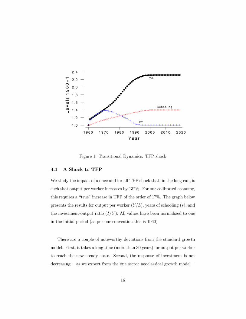
Figure 1: Transitional Dynamics: TFP shock

4.1 A Shock to TFP

We study the impact of a once and for all TFP shock that, in the long run, is

such that output per worker increases by 132%. For our calibrated economy,

this requires a “true” increase in TFP of the order of 17%. The graph below

presents the results for output per worker (Y/L), years of schooling (s), and

the investment-output ratio (I/Y ). All values have been normalized to one

in the initial period (as per our convention this is 1960)

There are a couple of noteworthy deviations from the standard growth

model. First, it takes a long time (more than 30 years) for output per worker

to reach the new steady state. Second, the response of investment is not

decreasing –as we expect from the one sector neoclassical growth model–

16

2 0 2 02 0 1 02 0 0 01 9 9 01 9 8 01 9 7 01 9 6 0

1 .5

1 .4

1 .3

1 .2

1 .1

1 .0

0 .9

Y e a r

Le

ve

ls 1

96

0 =

1

M e a s u re d TF PE ffe c tive H u m a n C a p ita l

M in c e r

Figure 2: TFP Shock. Effective Human Capital, Mincerian Human Capital,

and Measured TFP

but it increases for a period of 10 years, and then it goes back to its pre-

shock level over the next 20 years. The reason for this non-monotonicity

lies in the equilibrium response of effective human capital to a TFP shock.

Recall that, in the standard model, investment rises to induce the economy

to reach the new capital-labor ratio. This increase is moderated by higher

interest rates, but convergence is monotone. In the context of this model,

there is another force that induces the capital labor ratio to rise: a decrease

in the effective amount of human capital allocated to market production.

The behavior of effective human capital, he(t) = He(t)/N(6 + s(t); t), is

displayed in Figure 2.

17

The somewhat surprising finding is that effective human capital initially

decreases. This is due to two forces. First, there is a change in labor force

participation due to individuals choosing to acquire more schooling. Quan-

titatively this effect is a small (especially in the first 10 years). The second

force is that the increase, contemporaneous and expected, in real wages per

unit of human capital, induces more on the job training, especially among

younger individuals. Of course, the decrease in effective human capital re-

duces the capital-labor ratio and, consequently, requires a smaller level of

investment in physical capital.6

In Figure 2 we also report an alternative measure of human capital which

we label “Mincerian.” This notion, hm, is computed according to

hm(t) = hm0 eφs(t),

where φ is often associated with the return to education as estimated in a

Mincer regression. For this calculation we chose φ = 0.10, but the results

are very similar for slightly higher and lower values. We take s to the

the average years of schooling of the individuals in the work force. The

interesting observation is that Mincerian human capital is increasing from

the very beginning. Thus, an observer that studies the first 10 years after

the shock, would conclude that the return to education is very low.

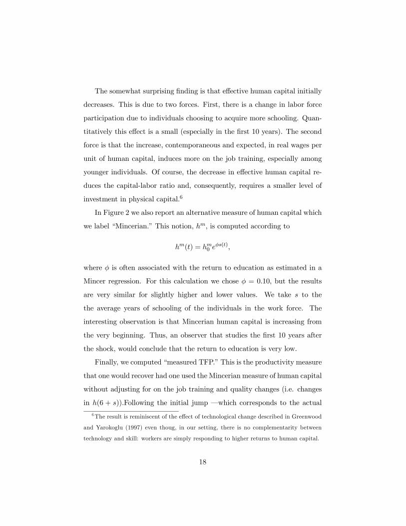
Finally, we computed “measured TFP.” This is the productivity measure

that one would recover had one used the Mincerian measure of human capital

without adjusting for on the job training and quality changes (i.e. changes

in h(6 + s)).Following the initial jump –which corresponds to the actual

6The result is reminiscent of the effect of technological change described in Greenwood

and Yarokoglu (1997) even thoug, in our setting, there is no complementarity between

technology and skill: workers are simply responding to higher returns to human capital.

18

change in TFP– this measure exhibits an upward slow trend. Using this

estimate one would conclude that productivity increased close to 50%, and

that it takes 25 years to reach 90% of its final value. Given the difference

between this measure and the actual path of TFP –which, of course, is

constant following an initial jump– we are hesitant to use existing measures

of productivity as driving shocks in the model.

It is easy to see how mismeasurement of human capital can account for

this behavior. Let ηx denote a growth rate of any variable x. Let effective

human capital per worker, he(t), be decomposed as

he(t) = h(t)eφs(t).

In this context, h(t) can be viewed as a measure of quality of human capital.

Simple algebra shows that the growth rate of measured TFP, z, is given by

ηz = ηz + (1− θ)ηh.

In our experiment, ηz = 0 after the first period. Consequently, standard

growth accounting would identify the change in quality as a productivity

improvement. This, of course, tends to overstate the quantitative impact of

any given productivity change.

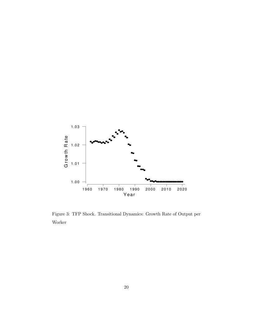
Given the one time shock that we study, the model predicts an instan-

taneous (and fairly large) jump in the growth rate. However, unlike the

standard model, it also implies a growth acceleration that occurs approxi-

mately 10 years into the experiment. For our parameterized economy the

relevant growth rate (omitting the first term) is displayed in Figure 3.

The growth rate remains constant (around 2%) for the first 10 years. It

increases up to 2.8% over the following 10 years, and then it decreases to

19

2020201020001990198019701960

1.03

1.02

1 .01

1 .00

Y ear

Gro

wth

Ra

te

Figure 3: TFP Shock. Transitional Dynamics: Growth Rate of Output per

Worker

20

its long run level of 0. The acceleration is being driven by the increase in

effective human capital (see Figure 2), corresponding to the higher quality

as a result of the previous investment in on-the-job training, and that the

new generations acquire more human capital per year of schooling.

Since changes in TFP cannot induce any changes in the capital-output

ratio, we now explore the role of demographic shocks that can, through their

impact on interest rates, generate such a change.

4.2 A Decrease in Population Growth

In this section we study a once and for all decrease in the log of the number

of children per person, f. We change f –the log of the number of children

per person– so that the population growth, η = f/B, which we take to

be initially 4%, decreases to 2%. This corresponds to to a decrease in the

fertility rate (2ef ) from 5.44 to 3.3. In this exercise we assume that the

average age of conception, B, is unchanged. This, is not neutral and in

future work we plan to explore the effect of changing B.

The results of this experiment for the base case are presented in Figure

4.

Unlike a TFP shock, a decrease in the number of children has a relatively

small effect in the short run: After 9 years output per worker has increased

only 10%. Investment in capital goods and years of schooling increase in the

same proportion. However, schooling expenditures relative to output (not

reported in the Figure) increases by 20 %, reflecting the anticipation of a

needed increase in quality.

After 20 years, the investment-output ratio settles into its new, long run

level which, for our parameterization, is 21% (the initial level was 17%).

21

2020201020001990198019701960

2.0

1.5

1.0

Year

Le

ve

ls 1

96

0 =

1

Y/L

Schooling

I/Y

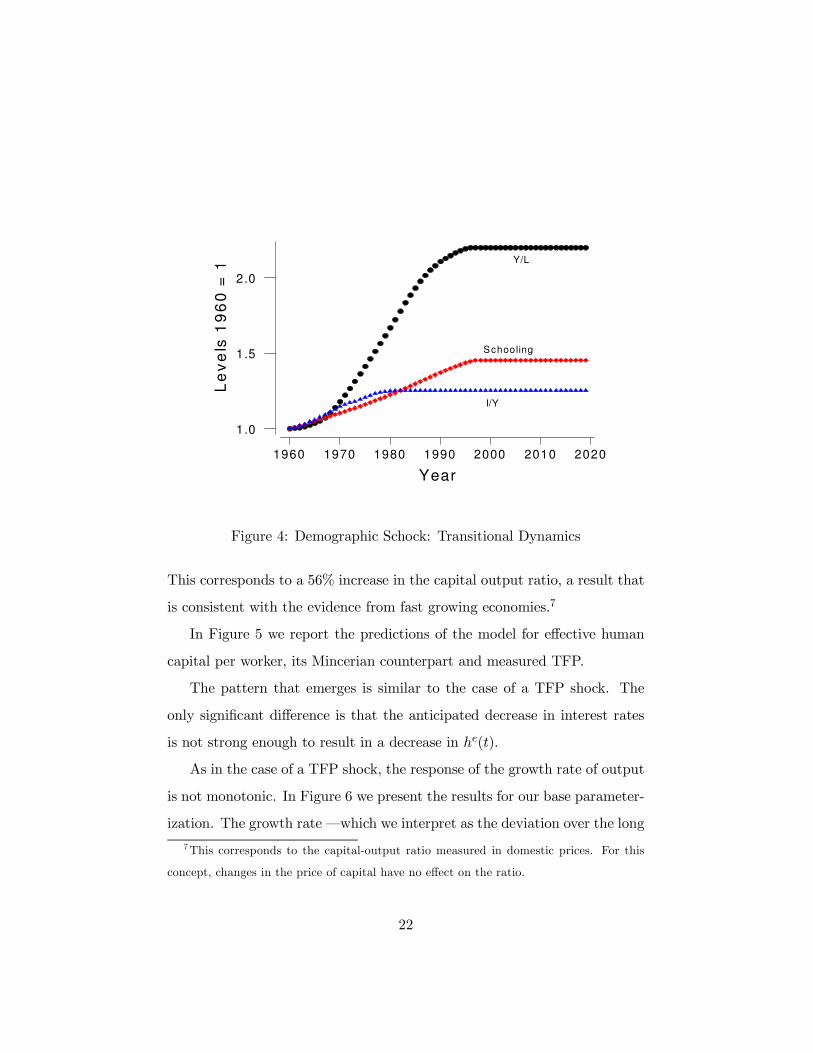
Figure 4: Demographic Schock: Transitional Dynamics

This corresponds to a 56% increase in the capital output ratio, a result that

is consistent with the evidence from fast growing economies.7

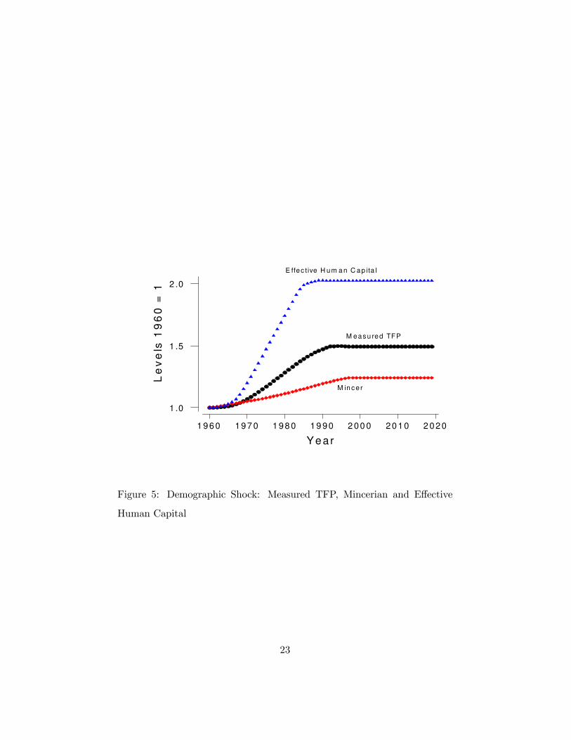
In Figure 5 we report the predictions of the model for effective human

capital per worker, its Mincerian counterpart and measured TFP.

The pattern that emerges is similar to the case of a TFP shock. The

only significant difference is that the anticipated decrease in interest rates

is not strong enough to result in a decrease in he(t).

As in the case of a TFP shock, the response of the growth rate of output

is not monotonic. In Figure 6 we present the results for our base parameter-

ization. The growth rate –which we interpret as the deviation over the long

7This corresponds to the capital-output ratio measured in domestic prices. For this

concept, changes in the price of capital have no effect on the ratio.

22

2 0 2 02 0 1 02 0 0 01 9 9 01 9 8 01 9 7 01 9 6 0

2 .0

1 .5

1 .0

Y ear

Le

ve

ls 1

96

0 =

1

M eas u red TFP

M in c e r

E ffec tive H um a n C ap ita l

Figure 5: Demographic Shock: Measured TFP, Mincerian and Effective

Human Capital

23

run growth rate– is fairly low for the first 7 years, but it accelerates in the

following 7 years. It peaks, at 3.5%, in year 14. The behavior of investment

and schooling (see Figure 4) cannot account for this. As in the previous case,

growth is influenced by changes in human capital quality. That is, growth

accelerates when the higher level of effective human capital is supplied to

the market sector.

2020201020001990198019701960

1.04

1.03

1.02

1.01

1.00

Year(G R )

Gro

wth

Ra

te

Figure 6: Demographic Shock: Growth Rate of Output per Worker

4.3 A Decrease in the Price of Capital

In this section we report the effect of a one time decrease in the price of

capital, pk, such that, in the long run, output per worker increases by 160%.

The results are displayed in Figure 7

24

2020201020001990198019701960

2.5

2.0

1.5

1.0

Year

Le

ve

ls 1

96

0 =

1

Y/L

Schooling

I/Y

Figure 7: Price of Capital Shock: Transitional Dynamics

Qualitatively, the predictions of the model are similar to those obtained

in the case of a TFP shock, both for levels and growth rate (See Figure 8)

4.4 Fast Growers: A First Pass

In order to obtain a more precise picture of the relative importance of TFP

and demographic shocks, we now study a version of their combined impact.

As a first pass to study the fast growing countries of East Asia, we cali-

brate the level of TFP (z) so that the predictions of the model for output

per worker relative to the U.S. matches the average of the East Asian fast

growing countries. We then analyze the effects of two shocks: a once and

for all TFP shock –as in the previous section– coupled with the actual

25

2020201020001990198019701960

1.04

1.03

1.02

1.01

1.00

Year

Gro

wth

Ra

te

Figure 8: Price of Capital Shock: Growth Rate of Output per Worker

changes in fertility. We pick the size of the TFP shock so that, in the long

run, output per worker displays a 7.7 fold increase (which corresponds to the

average increase in output per worker across the miracle economies). Our

demographic shock is such that the population growth rate decreases from

3.83% in 1960 to 1.68% in 2000, which is an average of the years surrounding

the beginning and the end of the period under study.

The results of this experiment are presented in Figure 9. Output per

worker evolves along an S-shaped path, which implies a delayed response of

the growth rate to the shocks. The reason is, as before, that it takes time

to accumulate human capital: After the economy is hit with a TFP shock,

agents find it optimal to increase their stock of human capital. New cohorts

26

go to school longer than did their older counterparts. Individuals who are

already working now engage in more on the job training. All this implies

that the stock of human capital takes time to respond. This slows down the

transition to the new steady state. The model is able to capture the rise in

schooling, as well as the dramatic rise in the investment to GDP ratio.

2020201020001990198019701960

8

7

6

5

4

3

2

1

Year

Le

ve

ls 1

96

0 =

1

Y/L

I/Y

Schooling

Figure 9: TFP and Fertility Shocks: Transitional Dynamics

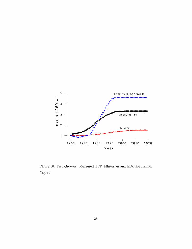
As in the case of the one time shocks, we use the model to estimate TFP

assuming a Mincerian human capital production function. The results are

in Figure 10. For this experiment, the increase in TFP induces a decrease

in effective human capital. It takes more than 10 years for he to get back to

its pre-shock level. In the mean time, the increase in output is due to the

TFP shock and capital accumulation.

27

2 0 2 02 0 1 02 0 0 01 9 9 01 9 8 01 9 7 01 9 6 0

5

4

3

2

1

Y ea r

Le

ve

ls 1

96

0 =

1

M e a s ure d TF P

M in c e r

E ffe c tive H u m a n C a p ita l

Figure 10: Fast Growers: Measured TFP, Mincerian and Effective Human

Capital

28

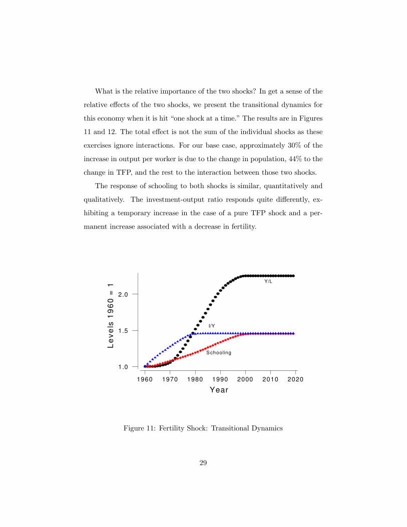
What is the relative importance of the two shocks? In get a sense of the

relative effects of the two shocks, we present the transitional dynamics for

this economy when it is hit “one shock at a time.” The results are in Figures

11 and 12. The total effect is not the sum of the individual shocks as these

exercises ignore interactions. For our base case, approximately 30% of the

increase in output per worker is due to the change in population, 44% to the

change in TFP, and the rest to the interaction between those two shocks.

The response of schooling to both shocks is similar, quantitatively and

qualitatively. The investment-output ratio responds quite differently, ex-

hibiting a temporary increase in the case of a pure TFP shock and a per-

manent increase associated with a decrease in fertility.

2020201020001990198019701960

2.0

1.5

1.0

Year

Le

ve

ls 1

96

0 =

1

Y/L

I/Y

Schooling

Figure 11: Fertility Shock: Transitional Dynamics

29

2020201020001990198019701960

3.5

3.0

2.5

2.0

1.5

1.0

Year

Le

ve

ls 1

96

0 =

1

Y/L

Schooling

I/Y

Figure 12: TFP Shock: Transitional Dynamics

30

If we interpret the effect of TFP as capturing transitional dynamics,

then we must conclude that transitional dynamics cannot be ruled out as

explanations for the growth performance of this group of countries.

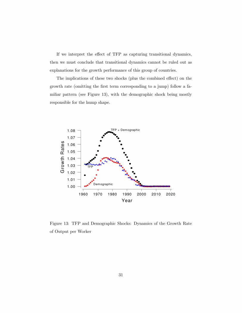
The implications of these two shocks (plus the combined effect) on the

growth rate (omitting the first term corresponding to a jump) follow a fa-

miliar pattern (see Figure 13), with the demographic shock being mostly

responsible for the hump shape.

2020201020001990198019701960

1.08

1.07

1.06

1.05

1.04

1.03

1.02

1.01

1.00

Year

Gro

wth

Ra

tes

TFP + Dem ographic

Dem ographic

TFP

Figure 13: TFP and Demographic Shocks: Dynamics of the Growth Rate

of Output per Worker

31

5 Growth Episodes

In this section we study how well the growth model can account for growth

episodes driven by technology shocks while taking into account demographic

changes. To this end, we choose the path of TFP for each country from 1960

to 2000 so that output per worker in the model matches a seven year moving

average in the data. We assume that TFP remains constant after 2000 (to

compute a steady state). Moreover, we change the demographic variables

to match each country’s data. We consider the closed economy case.

5.1 East Asia

We first consider the fast growing economies of East Asia. In particular, we

examine the implications of the model for Singapore, Hong Kong, Malaysia,

Taiwan and Korea. In all cases, we assume 1960 is a steady state (this turns

out not to be crucial).

The following table presents the results of the experiment. We report

the predictions for the total change in output per worker (which in this ex-

periment is perfectly matched by the model), the change in the investment-

output ratio, the change in actual (z) and measured (z)TFP (using the

methodology of the previous section), as well as the predictions for years of

schooling, when f is chosen to match measured fertility.

32

∆(Y/L) Years of Schooling ∆(I/Y) ∆(z) ∆(z)

Data Data Model Data Model Model Model

Country 1960 2000 1960 2000

Sing. 6.6 3.14 8.12 3.32 8.74 1.65 1.83 1.15 2.08

H.K. 9.09 4.74 9.47 4.42 8.95 0.89 1.91 1.20 2.71

Mal. 4.49 2.34 7.88 3.02 6.32 1.62 1.49 1.13 1.97

Taiwan 10.14 3.32 8.53 2.58 7.93 1.68 1.72 1.22 2.86

Korea 8.05 3.23 10.46 2.99 8.93 2.67 2.13 1.17 2.19

As can be seen, the model’s predictions for years of schooling in 2000 line

up reasonably well with the data. The predictions for the investment-output

ratio are also quite reasonable with one exception: Hong Kong. The reason,

in the context of the model, is simple: Lower fertility induces a decrease

in the interest rate and this, in turn, results in a higher investment-output

ratio (in the steady state). However, as is well known (e.g. Young (1992)),

the investment ratio in Hong Kong has not shown any trend.

An alternative approach to matching demographic change is to pick f

so that the model’s implication for the growth rate of population match

the data. This, it turns out, makes a significant difference. In Figures 14

and 15 we present for Hong Kong and Taiwan the time series for schooling

and the investment ratio implied by the model as well as actual schooling

(taken from Barro-Lee) for this case. It is clear that the model is consistent

with a substantial increase in schooling but it tends to overpredict schooling

in 1960. Thus, relative to the level of human capital, output was too low.

Since this crucially depends on the specification of demographic change we

will analyze this more carefully in the next version.

33

0

2

4

6

8

10

12

1955 1960 1965 1970 1975 1980 1985 1990 1995 2000 2005

Year

Yea

rs o

f S

ch

oo

lin

g

0

0.2

0.4

0.6

0.8

1

1.2

1.4

1.6

1.8

I/Y

(19

60

= 1

)

Schooling - Model

Schooling - Data

I/Y

Figure 14: Schooling and I/Y - Hong Kong

34

0

1

2

3

4

5

6

7

8

9

1955 1960 1965 1970 1975 1980 1985 1990 1995 2000 2005

Year

Ye

ars

of

Sc

ho

olin

g

0

0.2

0.4

0.6

0.8

1

1.2

1.4

1.6

1.8

I/Y

(1

96

0 =

1)

Schooling - Model

Schooling - Data

I/Y

Figure 15: Schooling and I/Y - Taiwan

35

5.2 The Latin American Experience

Is the model consistent with the Latin American experience? To analyze

the predictions of the model for each of the Latin American economies,

we conduct the same experiment between 1960 and 2000 and examine the

predictions for years of schooling and investment for both 1960 and 2000.

The results are in the following table.

GDP per worker Years of Schooling

Data Model

Country 1960 2000 1960 2000 1960 2000

Argentina 18732.67 25670.27 4.99 8.49 4.53 7.92

Bolivia 6811.40 6829.04 4.22 5.54 4.32 4.76

Brazil 7376.20 19220.33 2.83 4.56 2.55 5.31

Chile 11693.66 25083.56 4.99 7.89 4.01 7.24

Colombia 8240.58 11477.08 2.97 5.01 3.25 4.23

Costa Rica 11326.14 14826.86 3.86 6.01 3.45 5.14

Ecuador 6115.14 10903.19 2.95 6.52 2.67 5.26

Mexico 13357.17 24588.29 2.41 6.73 2.54 5.83

Paraguay 7366.88 10438.59 3.35 5.74 3.52 4.79

Peru 10087.53 10094.90 3.02 7.33 2.96 3.64

Uruguay 14484.33 21149.76 5.03 7.25 5.24 7.57

Venezuela 25292.39 17754.19 2.53 5.61 2.34 1.60

In most countries, the predictions of the model and the data are roughly

consistent. There are two notable exceptions: Peru and Venezuela. In

Venezuela, output per worker went down while schooling rose, while in Peru

output per worker stayed virtually constant while schooling rose.

36

On the other hand, in countries that did not experience extreme shocks

the results are reasonable, but by no means perfect. In particular, it seems

that the model tends to underpredict the increase in the years of schooling

in almost all the countries. This suggests that there may be other forces at

work.

We now present detailed results for two countries: Argentina and Chile.

2 0 0019 901 98 01 97 019 60

9

8

7

6

5

4

3

Y ear

Sc

ho

oli

ng

= Y

ea

rs,

I/Y

19

60

=3

S ch oolin g - M odel

Sch oolin g - D ata

I/Y (1 960 = 3)

Figure 16: Argentina: Schooling and Investment

In both cases the model seems to do a reasonable job of tracking the

changes in schooling, but it fails to reproduce the path of the investment-

output ratio. Unlike the fast growing countries of East Asia, TFP changes

play a minor role in the cases of Chile and Argentina. To be precise, the

total change (over a 40 year period) of actual (z) TFP is essentially 0 in

37

20001990198019701960

8

7

6

5

4

3

Year

Sc

ho

olin

g =

Ye

ars

, I/

Y 1

96

0=

3

Schooling - M odel

Schooling - Data

I/Y - M odel

Figure 17: Chile: Schooling and Investment

both Chile and Argentina. Total, over a 40 year period, growth in measured

TFP (z) 3.6% in Argentina and 2% in Chile. This absence of productivity

improvements coupled with a negative (albeit small) fertility shock results

in increasing investment-output ratios. The data show no trend in the case

of Argentina and a U-shape relationship in the case of Chile. In both cases,

investment is measured in domestic prices.

6 Opening up the economy

Up until now, we have considered the effects of exogenous changes in pro-

ductivity and demographics on the evolution of macroeconomic aggregates.

This, of course begs the question, what caused the miracle? What is behind

38

0

1

2

3

4

5

6

7

8

1950 1960 1970 1980 1990 2000 2010 2020 2030

Year

Va

lue

Output per Worker

Schooling Expenditures/GDP (%)

Years of Schooling

Figure 18: The Effect of Opening up the Economy

the TFP shock? In what follows, we examine the implications of opening

up the economy to world capital markets. In particular, we assume that

in 1960, the economy is closed. Suddenly, the economy is opened up and

the real interest rates now correspond to that of the American economy.

We then analyze the transitional path as the economy approaches the new

steady state.

There are a few noteworthy features of the effects of opening up the

economy. First, note that the aggregate consequences are large. Output

per worker increases by almost a factor of five. Second, the gains are not

immediate even though the economy is opened up all of a sudden. Finally,

39

this exogenous change increases investment in physical and human capital,

exactly the experience of the East Asian tigers. This experiment demon-

strates that a substantial part of the performance of the East Asian tigers

could well be attributed to the opening up of the economy.

7 Concluding Comments

In this paper we ask whether the Neoclassical paradigm is consistent with

the performance of the miracle economies. We find that it is. In particular,

we find that a standard Neoclassical set-up with finitely-lived individuals

who accumulate human capital is consistent with protracted transitions and

a rise in investments in human and physical capital. Unlike in the model

without human capital, a one time shock to productivity can generate ‘slow’

convergence to the new steady state. We also make some progress toward

understanding what caused the miracle. Preliminary results indicate that a

substantial part of the increase in output per worker could well have been

the consequence of opening up the economy.

40

References

[1] Ben Porath, Y., 1967, “The Production of Human Capital and the Life

Cycle of Earnings,” Journal of Political Economy 75, pt. 1, 352-365.

[2] Chang, Y. and A. Hornstein, 2007, “Capital-Skill Complementarity and

Economic Development,” working paper. [It is not a version that can

be quoted. Need to change.]

[3] Chen, K., A. Ïmrohoroglu, and S. Ïmrohoroglu, 2006, “The Japanese

Saving Rate,” working paper.

[4] Greenwood, J. and M. Yorukoglu, 1997, “1974,” Carnegie-Rochester

Series on Public Policy 46, pp: 49-95

[5] Hayashi, F. and E. C. Prescott, 2002, “The 1990s in Japan: A Lost

Decade,” Journal of Monetary Economics,

[6] Huggett M., Ventura G., and Yaron A. “Human Capital and Earnings

Distribution Dynamics,” working paper (2005).

[7] International Labour Organization, 2002, “Every Child Counts: New

Global Estimates on Child Labour," International Labour Office,

Geneva, April.

[8] King, R. G. and S. Rebelo, 1993,“ Transitional Dynamics and Economic

Growth in the Neoclassical Model,” American Economic Review, Vol.

83 pp: 908-931.

[9] Kurusçu, Burhanettin, 2006, “Training and Lifetime Income,” Ameri-

can Economic Review, forthcoming.

41

[10] Lucas, R. E., 1993, “Making a Miracle,” Econometrica, Vol. 61, No. 2,

pp: 251-272.

[11] Manuelli, R. and A. Seshadri, 2006, “Human Capital and the Wealth

of Nations,” working paper.

[12] Manuelli, R. and A. Seshadri, 2007, “Explaining International Fertility

Differences ,” working paper.

[13] Mincer, J., 1962, “On-the-Job Training: Costs, Returns and Some Im-

plications,” Journal of Political Economy, Vol. 70, No. 5 Part 2, pp:

50-79.

[14] Mincer, J., 1997, “The Production of Human Capital and the Life Cycle

of Earnings: Variations on a Theme,” Journal of Labor Economics, Vol.

15, Part 2, pp: S26-S47

42