neering - NASA · Skewed flat plate grid ..... 82 Friction coefficient, flat plate, skewed grid ..... 83 Velocity profile, flat plate, skewed grid ..... 84 Friction coefficient,

HTL- 55, CFD- 25Project 3335ISU-ERI-Ames-92259

D. L. Sondak R.H. Pletcher W.R. Van Dalsem

Wall Functions for thek- e Turbulence Model in Generalized

Nonorthogonal Curvilinear Coordinates

Final Report

Funds for the support of this study have been allocatedby the NASA-Ames Research Center, Moffett Field, California

under Interchange No. NCA2 - 526

Heat Transfer Laboratory

Department of Mechanical Engineering

Computational Fluid Dynamics Center

enqi .neeringresearch nst tute

iowa state university

ThL_ l.sa prepnn! ol a paper inle?.ded lot p_J_llCa_lOr'. ;1",_ lournal or proceedings Since Ct_c]es rr, c_ be r_._c_e be!ore pL.JZLIC_t:_ _'. L_.ISprepr:_ ! :_made available w_lh the undersland:r'.g _hat i!wl__.not be c_led or reproduced w_lhout the perm_sslor, c_ the _ut_,cr

https://ntrs.nasa.gov/search.jsp?R=19920016719 2018-07-14T16:07:37+00:00Z

°°°

111

TABLE OF CONTENTS

°°.

ABSTRACT ................................... xm

ACKNOWLEDGEMENTS ......................... xv

NOTATION .................................... xvii

1. INTRODUCTION ............................. 1

1.1 Problem Description ........................... 1

1.2 Historical Review ............................. 2

1.2.1 Turbulence modeling ....................... 2

1.2.2 Near-wall modeling ........................ 8

1.3 Scope of the Present Research ...................... 10

2. CONSERVATION OF MASS, MOMENTUM, AND ENERGY. 13

2.1 Introduction ................................ 13

2.2 Instantaneous Equations ......................... 13

2.3 Averaging Techniques ........................... 14

2.4 Mass-Averaged Transport Equations .................. 16

2.4.1 Continuity ............................. 17

2.4.2 Momentum ............................ 17

2.4.3 Energy ............................... 17

P'EC_E_I_'.)G PAGE BLAre1( NOT FILMED

iv

o

o

o

o

2.5 Closure Problem ............................. 19

k - e MODEL ................................ 21

3.1 Introduction ................................ 21

3.2 Turbulent Kinetic Energy Transport Equation ............. 24

3.3 Modeled Turbulent Kinetic Energy Equation .............. 26

3.4 Modeled Dissipation Rate Equation ................... 28

WALL FUNCTIONS ...........................

4.1 Background ................................

4.2 Detailed Formulation ...........................

Introduction ............................

Friction velocity ..........................

Boundary conditions for k and e .................

4.2.1

4.2.2

4.2.3

31

31

35

35

35

36

4.2.4

OTHER TURBULENCE MODELS ..................

5.1 Introduction ................................

5.2 Chien Low-Reynolds-Number Model ..................

5.3 BaJdwin-Lomax Algebraic Model ....................

NUMERICAL METHOD ........................

6.1 Nondimensional Equations ........................

6.2 Vector Form of Equations ........................

6.3

6.4

6.5

Application of _-_, to the Navier-Stokes equations ........ 40

53

53

53

55

57

57

58

Coordinate Transformation ........................ 61

Navier-Stokes Solver ........................... 66

k - e Solver ................................ 69

V

7. RESULTS .................................. 73

7.1 Introduction ................................ 73

7.2 Flat plate ................................. 74

7.2.1 Skewed grid ............................ 80

7.2.2 Angled domain .......................... 81

7.2.3 Low-Reynolds-number model test case ............. 84

7.3 Body of Revolution ............................ 90

7.3.1 Introduction ............................ 90

7.3.2 Fine grid .............................. 91

7.3.3 Medium grid ........................... 97

7.3.4 Coarse grid ............................ 102

7.4 Prolate Spheroid ............................. 102

7.4.1 Introduction ............................ 102

7.4.2 Grid ................................ 109

7.4.3 Boundary conditions ....................... 112

7.4.4 Additional considerations .................... 117

7.4.5 Results ............................... 120

8. CONCLUSIONS AND RECOMMENDATIONS .......... 135

9. REFERENCES ............................... 141

10. APPENDIX A: FLUX JACOBIANS ................. 151

10.1 Navier-Stokes ............................... 151

10.2 k - e .................................... 154

vi

11. APPENDIX B: k- e SOLVER ..................... 155

11.1 Banded Solver ............................... 155

11.2 Block Solver ................................ 158

vii

LIST OF TABLES

Table 4.1: Summary of shear stress transformations ........... 51

Table 7.1: Previous computations of DFVLR prolate spheroid ...... 110

ix

LIST OF FIGURES

Figure 4.1:

Figure 4.2:

Figure 4.3:

Figure 4.4:

Figure 4.5:

Figure 7.1:

Figure 7.2:

Figure 7.3:

Figure 7.4:

Figure 7.5:

Figure 7.6:

Figure 7.7:

Figure 7.8:

Figure 7.9:

Figure 7.10:

Figure 7.11:

Typical turbulent boundary layer velocity profile ....... 33

Definition of 7 coordinate direction .............. 41

Covariant base vectors ..................... 42

Example contravariant base vector ............... 43

Physical velocity components parallel to wall ......... 48

Orthogonal flat plate grid .................... 76

Friction coefficient, flat plate, orthogonal grid ......... 79

Velocity profile, flat plate, orthogonal grid ........... 79

Skewed flat plate grid ...................... 82

Friction coefficient, flat plate, skewed grid ........... 83

Velocity profile, flat plate, skewed grid ............. 84

Friction coefficient, flat plate, angled domain ......... 85

Velocity profile, flat plate, angled domain ........... 85

Flat plate grid, low-Reynolds-number model test case .... 87

Friction coefficient, flat plate, low-Reynolds-number model

test case ............................. 88

Velocity profile, flat plate, low-Reynolds-number model test

case ................................ 89

Eml,_,,V_,,_il. II_N"I_N,_v _,_,_ PRECEDING PAGE BLANK NOT FILMED

X

Figure

Figure

Figure

Figure

Figure

Figure

Figure

Figure

Figure

Figure

Figure

Figure

Figure

Figure

Figure

Figure

Figure

Figure

Figure

Figure

Figure

Figure

Figure

7.12:

7.13:

7.14:

7.15:

7.16:

7.17:

7.18:

7.19:

7.20:

7.21:

7.22:

7.23:

7.24:

7.25:

7.26:

7.27:

7.28:

7.29:

7.30:

7.31:

7.32:

11.1:

11.2:

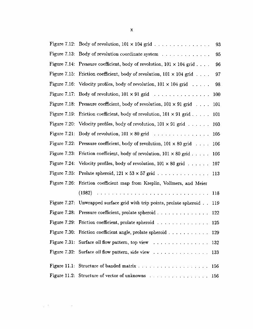
Body of revolution, 101 x 104 grid ............... 93

Body of revolution coordinate system ............. 95

Pressure coefficient, body of revolution, 101 x 104 grid .... 96

Friction coefficient, body of revolution, 101 x 104 grid .... 97

Velocity profiles, body of revolution, 101 x 104 grid ..... 98



Friction coefficient, body of revolution, 101 x 91 grid ..... 101

Velocity profiles, body of revolution, 101 x 91 grid ...... 103



Friction coefficient, body of revolution, 101 x 80 grid ..... 106

Velocity profiles, body of revolution, 101 x 80 grid ...... 107

Prolate spheroid, 121 x 53 x 57 grid .............. 113

Friction coefficient map from Kreplin, Vollmers, and Meier

(1982) .............................. 118

Unwrapped surface grid with trip points, prolate spheroid . 119

Pressure coefficient, prolate spheroid .............. 122

Friction coefficient, prolate spheroid .............. 125

Friction coefficient angle, prolate spheroid ........... 129

Surface oil flow pattern, top view ............... 132

Surface oil flow pattern, side view ............... 133

Structure of banded matrix ................... 156

Structure of vector of unknowns ................ 156

xi

Figure 11.3: Structure of right hand side ................... 157

Figure 11.4: Structure of block matrix .................... 159

0.,

Xlll

ABSTRACT

Wall functions are often employed to model turbulent flow near solid walls. A

method has not been available, however, for the application of wall functions to

generalized curvilinear coordinate systems, particularly those with nonorthogonal

grids. A general method for this application is developed herein.

A k - e turbulence model suitable for compressible flow, including the new wall

function formulation, has been incorporated into an existing compressible Reynolds-

averaged Navier-Stokes code, F3D. The low-Reynolds-number k - e model of Chien

(1982) was added for comparison with the present method. A number of features

were also added to F3D, including improved far-field boundary conditions and viscous

terms in the streamwise direction.

A series of computations of increasing complexity was run to test the effectiveness

of the new formulation. Flow over a flat plate was computed using both orthogonal

and nonorthogonal grids, and the friction coefficients and velocity profiles compared

with a semi-empirical equation. Flow over a body of revolution at zero angle of attack

was then computed to test the method's ability to handle flow over a curved surface.

Friction coefficients and velocity profiles were compared to test data. The same case

was also computed using the Chien (1982) low-Reynolds-number k - e model and the

Baldwin-Lomax (1978) algebraic model for comparison. All three models gave good

xiv

results on a relatively fine grid, but only the wall function formulation was effective

with coarser grids. Finally, in order to demonstrate the method's ability to handle

complex flowfields, separated flow over a prolate spheroid at angle of attack was

computed, and results were compared to test data. The results were also compared

to the computation of Kim and Patel (1991), in which a k - e model with a one-

equation model patched in at the wall was employed. Both models gave reasonable

solutions, but they require improvement for accurate prediction of friction coefficients

in the separated regions.

XV

ACKNOWLEDGEMENTS

The authors gratefully acknowledge the support provided for this research under

NASA Ames Research Center contracts NCC2-476 and NCA2-526. Special thanks

also goes to Dr. I.-T. Chiu for his help in setting up formats for figures and tables

in this report, and also for his help in exorcising various computer-related gremlins

along the way.

xvii

NOTATION

Roman Symbols

a

A,B,C

ai

a i

b

B

at

%

c_

CI

Ckleb

C1

C2

C3

speed of sound

flux Jacobian matrices

covariant base vector

contravariant base vector

proportionality constant between metrics

constant for law of the wall, 5.0

constant for Norris and Reynolds near-wall length scale equation

specific heat at constant pressure

constant for k - e model, 0.09

constant for Baldwin-Lomax model, 1.6

friction coefficient





constant for Chien model, 0.0115

PRECEDING PAGE BLANK NOT FILMED

..°

XVI11

C4

D

D

7)

ei

e_, f_, g_

E, F, G

E,,,Fv,G,_

£

I

Fkleb

Fwake

G

h

H

1-1,

J

k

K¢

K

l

l,

.,V

constant for Chien model, 0.5

dissipation term in turbulent kinetic energy transport equation

k - e source term Jacobian matrix

smoothing operator

unit covariant base vector

energy equation fluxes

inviscid flux vectors

viscous flux vectors

total internal energy per unit volume

damping function for Chien model

Klebanoff intermittancy function, for Baldwin-Lomax model

Klebanoff wake function, for Baldwin-Lomax model

metric tensor

metric matrix

static enthalpy per unit mass

total enthalpy per unit mass

source term vector for turbulence transport equations

Jacobian of coordinate transformation

turbulent kinetic energy

Clauser constant for Baldwin-Lomax model, 0.02688

geometric stretching ratio

length scale

near-wall length scale of Norris and Reynolds

defined by equation (6.83)

XIX

n

P

P

P

Pr

Prt

q

Q

r

R

Re

Ret

Re_

Re_

8

S

S

T

T

T

To

coordinate direction normal to wall

static pressure

production of turbulent kinetic energy

term proportional to production of turbulent kinetic energy

physical shear stress matrix

Prandtl number, 0.72

turbulent Prandtl number, 0.9

heat transfer rate

dependent variable vector

position vector

gas constant

Reynolds number based on freestream speed of sound

turbulent Reynolds number

Reynolds number based on freestream velocity and reference length

Reynolds number based on freestream velocity and distance from

virtual origin

spectral radius of inviscid flux Jacobian

constant for Sutherland's law

diagonal matrix containing functions of metrics

static temperature

matrix, columns of which are right eigenvectors of inviscid flux

matrix

shear stress matrix


XX

t

U

u, V, W

U +

u.

u,v,w

W

x, y, z

Y

y+

Z

time

velocity parallel to wall (2-D examples)

velocity components in physical coordinate directions

velocity normalized by friction velocity

friction velocity

physical velocity component in a direction

contravariant velocity components

Coles' wake function

physical coordinate directions

coordinate direction normal to wall (2-D examples)

distance from wall in wall coordinates

point where viscous sublayer intersects log region,

neglecting buffer region

function of Cf, defined by equation (7.9)

Greek Symbols

7

7

7

6_j

function to switch from fourth to second order smoothing

near shocks

ratio of specific heats, 1.4

coordinate direction normal to wall

friction coefficient angle

Kronecker delta

xxi

A

E

E2

E4

E

A

#o

#h

_t

V

v_

P

Gk

Y

central difference operator for inviscid fluxes

boundary layer thickness

central difference operator for viscous fluxes

forward difference operator

dissipation rate of turbulent kinetic energy

second difference smoothing coefficient

fourth difference smoothing coefficient

total internal energy per unit mass

circumferential angle

velocity scale

Von Karman constant, 0.41

diagonal matrix containing eigenvalues of inviscid flux Jacobian

molecular viscosity


turbulent diffusion coefficient for static enthalpy

turbulent viscosity

kinematic viscosity

diffusion coefficient for passive scalar

transformed coordinates

constant for Coles' law of the wake, 0.5

density



shear stress

xxii

physicalshearstresscomponentsin a,/? directions

vorticity

Subscripts

exp

i,j,k,t

imp

ref

t

W

X_ y_ Z

explicit

tensor indices

implicit

reference

turbulent

viscous

wall

partial differentiation in physical coordinate directions

tensor indices

freestream

Superscripts

n

v

+

÷

time level

viscous

wall variable

positive eigenvalue

negative eigenvalue

°°°

XXIll

I

II

fluctuating quantity, Reynolds average

fluctuating quantity, Favre average

Other Symbols

V

V

backward difference operator

gradient operator

time average

tensor in transformed coordinates

modified by wall functions

mass-weighted average

vector in transformed coordinates, conservation law form

1. INTRODUCTION

1.1 Problem Description

The understanding of turbulence is of critical importance for the prediction of

flows encountered in many important engineering applications such as flow over flight

vehicles, impingment cooling in industrial processes, and the transport of atmospheric

pollutants. In principle, these flowfields could be predicted by solving the full Navier-

Stokes equations. This approach is not practical, however, since present computers

do not have the speed and memory required to resolve the wide range of length and

time scales in most turbulent flows. In practice, the Navier-Stokes equations are

employed to resolve large scales, and turbulence models are relied upon to simulate

the effects of the small-scale motion.

Turbulence is diffusive, and most approaches to turbulence modeling are directed

toward computing the rates of turbulent diffusion of momentum and energy. Unfor-

tunately, a general method for determining these diffusion rates has proven elusive.

Turbulence models have been developed which work well for certain classes of flows,

but their range of applicability is limited. Some models, for example, work well for

attached flows, but perform poorly in regions of separated flow.

Aside from the generality of turbulence models, another concern is the amount

of computing power required to apply them. Computations of complex flows may

2

require millions of grid points and hundreds of hours of CPU time, even on the

fastest availablecomputers. It is thereforeimportant to considerboth accuracyand

computing requirementsin the developmentand application of turbulence models.

1.2 Historical Review

1.2.1 Turbulence modeling

The earliest attempt to analyze the turbulence problem is usually attributed to

Reynolds (1895). He was trying to explain the result of his famous transition exper-

iment in which he showed that pipe flow becomes turbulent at a distinct Reynolds

number. Being familiar with the kinetic theory of gases, Reynolds tried an analo-

gous approach for fluid flow, decomposing velocities into mean and fluctuating parts.

When expressions for the decomposed velocities were substituted into the Navier-

Stokes equations, a set of additional terms appeared. These terms are the gremlins

which we now call the Reynolds stresses, and the subsequent ninety years or so have

been littered with attempts to find a general method of predicting their values.

Since viscous stress in a Newtonian fluid is a linear function of the velocity

gradient, it was hypothesized that Reynolds stresses behave in the same manner.

Unfortunately, determining the proportionality constant, the turbulent viscosity, at

first proved to be as intractable as determining the Reynolds stresses themselves.

In the 1920s, it was shown that transport equations could be written for moments

of arbitrary order (Monin and Yaglom 1987). However, each equation for a specified

moment contains the next higher moment as an unknown. For example, the equations

for the Reynolds stresses, which are second order moments (the correlation between

two velocity components), contain third order moments (the correlation between

three velocity components)as unknowns. This is the "closure problem" and was a

harbinger of difficulties to come.

Someheadway was achievedby Prandtl's "mixing length" hypothesis. It is

interesting to note that Prandtl, like Reynoldsbeforehim, turned toward the kinetic

theory of gasesfor inspiration. According to the kinetic theory, kinematic viscosity

is proportional to the product of a velocity scale(the rms velocity of the molecules)

and a length scale (the mean free path of the molecules)(Hinze 1987). Treating

"lumps of fluid" like molecules,Prandtl hypothesizedthat the turbulent viscosity is

alsoproportional to the product of a velocity scaleand a length scale.Unfortunately,

the analogywith molecularmotion is onshakygroundat best. Moleculesretain their

identity, while lumps of fluid do not. Also, the length scaleof molecular motion is

small comparedto the overall system, and this is not the case for turbulent fluid

flow (Tennekesand Lumley 1972). Evenwith theseweaknesses,the mixing length

theory hasprovento be usefulfor the prediction of simpleflowfieldssuchasfreejets

and boundary layers on flat plates. Its main drawback is that the proportionality

constant must be determined empirically, and a given constant is useful only for a

very limited classof flows.

An approachvery different from mixing length theory wastaken by G. I. Taylor

(1935). Sincethe Reynoldsstressesareexpressedascorrelationsbetweenfluctuating

componentsof velocity, it was natural to apply statistical methods to attempt to

find general expressionsfor thesecorrelations. Taylor developedthis method for

isotropic and, to a lesserdegree,homogeneousturbulence. A great deal of insight

into the mechanismsof turbulent energytransfer hasbeengleanedfrom this work.

Its application to usefulturbulencemodelshasbeenlimited, though, sinceturbulence

is not actually isotropic, and only approximates homogeneity for certain very simple

flows, such as wind tunnel turbulence behind a grid.

While statistical methods were being developed, other approaches to improving

upon mixing length theory were investigated. One of the disadvantages of mixing

length models is that they do not account for "history" (transport) effects on the

turbulence. To alleviate this shortcoming, one or more transport equations can be

employed. It is possible to derive an exact equation for the transport of turbulent

kinetic energy, although additional unknowns are introduced in the process. The new

unknowns can be modeled, and the resulting equation can be used to deduce a ve-

locity scale distribution of the turbulence. Specification of a length scale distribution

then closes the problem. If the length scale is calculated algebraically, the resulting

model is known as a "one-equation model," since one partial differential equation is

employed.

One-equation models yield better results than mixing length models for flows in

which convection and diffusion of turbulent kinetic energy are important (Launder

et al. 1972). For many complex flows, however, algebraic specification of the length

scale can be difficult. The next logical step would therefore be to develop a transport

equation for length scale, or a quantity which can be easily related to a length scale.

This equation, along with the turbulent kinetic energy transport equation, yields a

two-equation model. The second equation is usually written for the rate of dissipation

of turbulent kinetic energy, e, although other quantities are sometimes used, such as

the length scale, L, (Rodi and Spalding 1970), the rate of dissipation per unit energy,

w, (Wilcox 1988), and the time scale, r (Abid, Speziale, and Thangam 1991). Two-

equation models came to the forefront upon publication of a series of papers from Los

5

Alamos Scientific Laboratory (Harlow and Nakayama 1967; Harlow and Nakayama

1968; Daly and Harlow 1970). Derivation of the second equation is not as rigorous

as that of the turbulent kinetic energy equation, and this is often cited as a point of

weakness of two-equation models. Even so, calculation of the length scale as part of

the model has proven to be advantageous for many flowfields.

Daunted by the prospect of solving the complete second-moment equations

and searching for a method to improve the performance of two-equation models,

Rodi (1972) investigated the possibility of simplifying the second-moment equations.

He developed an algebraic expression for the Reynolds stresses as a function of the

dependent variables in his two-equation model, and the model is therefore referred

to as an algebraic Reynolds stress model. Since the new equation is algebraic, little

computational effort is required above that for the two-equation model. Although

algebraic Reynolds stress models show promise, they have not exhibited the expected

improvements over two-equation models (Ferziger 1987).

Other variations of two-equation models have also been investigated. One weak-

ness of two-equation models is that a single velocity scale and a single length scale

are assumed to be sufficient to describe the turbulence. This implies that the energy

spectrum is similar in different regions of the flowfield, which is not generally true.

In "multiscale" two-equation models, the energy spectrum is divided into two parts

(Launder 1979). The first is the production range, which is the region of highest

energy. The second is the transfer range, where the energy is transferred from large

scales to small scales. Separate k and e transport equations are written for each range.

Multiscale models have shown improvements over standard two-equation models for

flowfields such as flow over a backward-facing step (Kim and Chen 1989) and swirling

jets (Ko and Rhode 1990). The results are not consistentlybetter, however,and a

significant increasein computer poweris requireddueto the addition of two transport

equations.

Another variation of two-equation models is the "nonlinear" model. In some

flowfields, anisotropy of the normal turbulent stressesis important. An exampleof

this is the secondaryflow observedto occur in turbulent flow through straight rect-

angular channels.Sincethe Boussinesqapproximationdoesnot admit anisotropyof

the normal turbulent stresses,it is impossibleto predict thesesecondaryflowswith

the standard model. In nonlinear models(Speziale1987;Yoshizawa1988; Barton,

Rubinstein, and Kirtley 1991),the Boussinesqapproximation is replacedby a nonlin-

ear function of the meanstrain rate. This method is not restricted to two-equation

models,but can be appliedto other modelswhich utilize the Boussinesqapproxima-

tion (e.g., algebraicmodels). Initial results from thesemodels look promising, but

moreapplicationsneedto be investigatedbeforetheir valuecanbe fully assessed.

As mentioned above,the closureproblem precludesthe solution of the trans-

port equationsfor correlationsbetweenfluctuating velocity components.Also, these

equationscontain terms suchas pressure-velocitycorrelations,which are generally

unknown. Chou (1945) made various assumptions about the unknown quantities in

the second and third moment transport equations in order to close them, creating

what is now referred to as a Reynolds stress transport model. An advantage of this

type of model is that the Boussinesq approximation is not employed. Although the

Boussinesq approximation is effective for many types of flows, it is known to be in-

accurate for some flowfields such as wall jets. Chou's model laid fairly dormant for

many years, because means for solving the equations for general cases were not avail-

able. As computerscameinto prominenceand improvedin capability, greater efforts

wereput into the developmentof Reynoldsstressmodels. Thesemodels require a

greatdeal of computational effort, and they do not presentlyyield resultswhich are

generallybetter than two-equationmodels.As they are further refined,it is expected

that they will comeinto greater usein the future.

The goalof all techniquesdiscussedsofar is to computethe Reynoldsstresses.

The Reynoldsstressesrepresentmomentum transfer averagedover a wide range of

scales. If a flowfield is computed using a very fine grid, large-scalestructures can

be resolved,and only the momentumtransfer occuringat smaller scalesneedsto be

modeled. Since the required model representsa subsetof the full range of scales,

it can be simpler in form than modelswhich representthe full Reynoldsstresses.

This approach is called "large eddy simulation." The disadvantageof large eddy

simulation is the great amount of computer powerrequired to run with sucha fine

grid. This method is thereforepresentlyconstrainedto relatively simple flowfields.

In theory, a grid could be constructed which is fine enough to resolve the full

spectrum of scales encountered in turbulent motion, obviating the need for any turbu-

lence model at all. This approach, "direct numerical simulation," has been applied to

very simple geometries at low turbulent Reynolds numbers (e.g., Rai and Moin 1989).

Since a doubling of the turbulent Reynolds number requires an order-of-magnitude

increase in computer capability (Yakhot and Orszag 1986), it will not be possible to

use direct simulation to solve "real world" problems in the near term future. It has

been estimated that if a terra.flop (1012 floating point operations per second) machine

were available, several hundred thousand years of CPU time would still be required

to compute a direct simulation of flow over an entire aircraft (Peterson et al. 1989).

This would prove to be a major annoyanceto typical computer system managers,

and is thereforeuntenable. Evenso,presentdirect simulation resultsarevaluablefor

studying the detailed structure of turbulence. Quantities which arenot measurable

can be extracted from the simulation results, and this is an excellentway to check

details of turbulence models.

1.2.2 Near-wall modeling

As solid walls are approached, the structure of turbulent flow changes due to the

increasing importance (and eventual dominance) of viscous effects. Many turbulence

models have been developed with the assumption that the flow is fully turbulent (i.e.,

far from walls), and they require additional attention in order to model wall regions

correctly.

An early near-wall model which has proven quite useful, and often appears today

in many guises, is that of Van Driest (1956). Van Driest was looking for a way to

modify the Prandtl mixing length to account for damping of turbulent eddies near

walls. He noted that in Stokes' solution for flow over an oscillating flat plate, the

amplitude of motion falls off exponentially with distance from the plate. This function

may be interpreted as quantifying the region of viscous influence. Van Driest used a

similar function to damp the mixing length near walls, since turbulent effects decrease

as viscous effects increase.

As more complex turbulence models came into use, new approaches to modeling

near-wall behavior were required. Most of these near-wall models attempt to approx-

imate the effects of anisotropy, which are neglected elsewhere in the flowfield. These

models are sometimes referred to as "low-Reynolds-number models," since they come

into play in regionsof low turbulent Reynoldsnumber. Harlowand Nakayama(1967)

presenteda tentative anisotropy correction to the turbulent kinetic energy in their

two-equation model, but they showedno results. Daly and Harlow (1970) used a

"wall-effecttensor" to modify the fluctuating pressure/strainrate correlation term in

their Reynoldsstressmodel. They showedthat this term drove the peak turbulent

kinetic energycloserto the wall asthe Reynoldsnumber increased,which is in accord

with experimentaldata.

A different approach, "wall functions," wasapplied by Patankar and Spalding

(1970). They reasonedthat equationsdescribingthe structure of turbulent boundary

layers,e.g., the law of the wall, could be coupledwith numerical solution schemes,

thereby eliminating the needto resolvethe turbulent boundary layer in the region

where anisotropy is important. This techniqueis limited by the accuracyand range

of applicability of the equationsemployed.

An early two-equation near-wall model which has been quite influential is that

of Jones and Launder (1972). They interpreted the e transport equation as modeling

only the isotropic part of the dissipation rate. Using asymptotic analysis, a term was

added to the turbulent kinetic energy transport equation to account for anisotropy

of the dissipation rate. Damping functions were employed for several terms in the e

equation, and an ad-hoc term was added to bring the maximum level of turbulent

kinetic energy into line with experimental data.

Development of both wall functions and low-Reynolds-number models has con-

tinued in parallel. Chieng and Launder (1980) refined the computation of the wall

shear stress, and their approach has been implemented by many investigators. Their

method was further generalized for compressible, separated flow by Viegas, Rubesin,

10

and Horstman (1985). Chien (1982) took an approach similar to that of Jones and

Launder (1972) to create a low-Reynolds-number model which has gained wide accep-

tance. There has been a great deal of activity in recent years in the development of

improved low-Reynolds-number models, usually based on asymptotic analysis. A use-

ful comparison of eight of these models is given by Patel, Rodi, and Sheuerer (1985),

where it is concluded that even the best performing models need more development

if they are to be used with confidence. Avva, Smith, and Singhal (1990) directly

compared results of wall functions and a common low-Reynolds-number model for

three two-dimensional flowfields, and found that wall functions gave comparable or

better results in all three cases.

The best choice between the two techniques has yet to be conclusively deter-

mined. Wall functions yield good results for many problems, and they require less

computer power than low-Reynolds-number models. Low-Reynolds-number models

have the potential to be more general and to give better results for some flowfields,

but that potential has yet to be demonstrated. Both approaches will most likely

continue to be used in the future.

1.3 Scope of the Present Research

One disadvantage of wall functions is that they are difficult to apply to complex

geometries. Early applications generally involved two-dimensional flows over flat

surfaces such as duct flows, backward-facing steps, and compression corners. Com-

putation of flow over complex three-dimensional geometries is now commonplace, but

a method for applying wall functions to these geometries has not been available. In

the present work, a method has been developed for the application of wall functions

11

to three-dimensionalgeneralizedcurvilinear coordinateswith nonorthogonal grids.

A high-Reynolds-numberk - e turbulence model with the new wall function for-

mulation has been added to F3D, a Reynolds-averaged compressible Navier-Stokes

solver. F3D utilizes an implicit, partially flux-split, two-factor approximate factor-

ization algorithm, and the ke model utilizes an implicit, fully flux-split, three-factor

approximate factorization algorithm. The Chien (1982) low-Reynolds-number k - e

model has also been added for comparison with the wall function formulation. F3D

contains the Baldwin-Lomax (1978) algebraic turbulence model, which was also run

for comparison with the present method.

The new wall function technique was applied to a series of test cases. First, flow

over a flat plate was computed using two different grids, one which is orthogonal

and one which is skewed at the wall, to test the nonorthogonal grid capabilities of

the present formulation. For these cases, the computed friction coefficients were

compared with those from a semi-empirical equation. Velocity profiles were also

compared with experimental data.

Flow over a body of revolution at zero angle of attack was then computed to

show the method's effectiveness for flow over a curved surface. Friction coefficients

and velocity profiles were compared with test data. The same case was also computed

using the Chien (1982) low-Reynolds-number k - e model and the Baldwin-Lomax

(1978) algebraic model for comparison. Each of the cases was run on three grids

with different wall spacings, demonstrating the advantage of wall functions for coarse

grids.

Finally, flow over a prolate spheroid at angle of attack was computed using the

wall function formulation, and results were compared with test data. This demon-

12

strated the effectivenessof the wall function formulation for a complexflowfieldwith

regions of separated flow.

13

2. CONSERVATION OF MASS, MOMENTUM, AND ENERGY

2.1 Introduction

For turbulent flows, it is not possible to solve the equations of motion numerically

due to the immense computer power which would be required to resolve the wide range

of length scales. In order to make the problem tractable, the equations are averaged

in time, introducing additional unknowns. The additional unknowns, which represent

turbulent transport of momentum and energy, are then modeled using a combination

of analysis and empiricism. In this chapter, the technique for averaging fluctuating

quantities is presented, and it is then applied to the equations of motion.

2.2 Instantaneous Equations

The working fluid is assumed to be a homogeneous continuum, and therefore

may not contain voids or particulates. It is also assumed that the fluid is Newtonian,

i.e. that the stress is proportional to the rate of strain. Stokes' hypothesis that the

bulk and molecular viscosities ()_ and /_ respectively) are related by the equation

= -(2/3)p is employed. Finally, buoyancy and other body forces are neglected.

Given these assumptions, the equations of conservation of mass per unit volume,

14

momentum per unit volume, and total enthalpy per unit volumeare givenby

Op+ 0-_xj(puj)= o (2.1)

_-(p_,)+_(p_,_ +_,_p-_,_)=o (2.2)

_(pH- p)+_(,_z +q_- =,,,_)=0 (2.3)O_ VX3

where

(0u, 0u_ 2 0uk_ (2.4)

This is a system of five equations with seven unknowns, and must be closed with

the aid of an equation of state and an expression for molecular viscosity. The fluid

is assumed to be a perfect gas,

p = pnT (2.5)

where temperature is related to total enthalpy by

H 1 (2.6)- h+ _(uiui)

1 (2.7)= cvT+ _(uiui)

The molecular viscosity will be calculated from Sutherland's Law (White 1974),

(Z'_/_T__o_+_s_--_. (2.8)I_o \To] T + S

where for air, #0 = 0.1716mP, To = 491.6°R, and S = 199°R.

2.3 Averaging Techniques

Following Reynolds' approach toward dealing with turbulent flow, values of ve-

locity and fluid properties are decomposed into mean and fluctuating parts. There are

15

two commontechniquesof decomposition,"Reynoldsaveraging"and "mass-weighted

averaging." Reynoldsaveragingis usually employedfor incompressibleflows, while

mass-weightedaveragingis more convenientfor compressibleflows. Here, the word

"average"will be usedto refer to averagingover time, definedby

- 1 /,',+A,¢d,.¢= (2.9)

where ¢ is the quantity being averaged, and t is time. In practice, the time must be

large with respect to the fluctuation time scale, but small with respect to the time

scale of global changes in the mean flowfield.

The mass-weighted average is defined by

(2.1o)

where p represents density, and the tilde is used to indicate a mass-weighted average.

In Reynolds decomposition, quantites are decomposed into mean and fluctuating

parts as follows:

¢=¢+¢' (2.11)

where ¢ is the instantaneous value of the quantity being averaged, 7 is defined by

equation (2.9), and ¢' is the fluctuating part of ¢. The analogous equation for mass-

weighted averaging is

¢=¢+¢" (2.12)

Now several useful properties of these averages will be developed. First averages

of fluctuating components will be examined. From equations (2.9) and (2.11),

16

-- 1 [t+At¢' - At.,, (¢- -_)dr

1 ['+_'¢dr l['+z_'-¢dr= -_. --_.

=¢-¢

= 0 (2.13)

For mass-weighted averages,

1"_ Jt

1 it+at_ p(¢--¢)dTAt .It

-- At Jt A-t J,

=

From equation (2.10),p--¢= _, so

p¢i-'7= 0 (2.14)

m

It is important to note that (I/'_=0.

2.4 Mass-Averaged Transport Equations

The variables in the continuity, momentum, and energy equations will now be de-

composed into average and fluctuating components, and the results averaged. Equa-

tion (2.11) will be used to decompose p, p, and r, and equation (2.12) will be used

for uj and H.

2.4.1

17

Continuity

Decomposing the variables in the continuity equation (2.1) and averaging yields

O _ u'j)_(_--4-Z)+ b-_zjp(_j+ = 0

Applying equations (2.13) and (2.14),

0 0 .

_+ _xj(Zuj) = 0

2.4.2 Momentum

Decomposing and averaging the momentum equation (2.2) yields

(2.15)

(2.16)

(2.17)


_---(PUi) + _-_xj[puiuj + 6ij_- (_ij - pu_'u;)] = 0 (2.18)

2.4.3 Energy

Decomposing and averaging the energy equation (2.3) yields

_-[p( + g") - (_ + p')]#

+ .[p(aj+ u_)(H+ H")+ (_, + _) - (as+ u_)(_,_+ gj)] = 0 (2.19)


0 - O - _

-_(-_H - _) + _xj [-_ajH + puSH" + _j - ,5,e,j - u_'ni] = 0 (2.20)

18

II

It will be useful to express H" in terms of h", fii, ui, p, and p. From the definition

of total enthalpy,

H1

-- h + _uiu i (2.21)

1

= h + h" + _ (fii + u'i')(fii + uT) (2.22)

1,,,,,= h + _tifii + h" + _u i u i) + fiiu 7 (2.23)

The definition of mass-average, equation (2.10), applied to the total enthalpy gives

= pH (2.24)

D

i

p (h + ½uiu,) (2.25)

h + ½p(_''+ uT)(ai+ _7) (2.26)

1 _ _ 1 --- II- IIvui ui (2.27)

Subtracting equation (2.27) from equation (2.23) yields an expression for the fluctu-

ating component of total enthalpy,

1 . IIH" = h" + _u i u i

1 __It_ Itp'u i "ai

2 -_- " (2.28)+ uiu i

Applying this equation to equation (2.20) yields

0 - 0 [ -- 1 ,, ,,. ]-_(-fiH - _) + _ I.Trfj[-'I + push" + "qj - fii('_ij - pu:'C;) - u;'(rij - 5pu,u_)j = o

(2.29)

If the boundary-layer approximation is used, the last term on the left hand side may

be neglected (Cebeci and Smith 1974; Anderson, Tannehill, and Pletcher 1984). It is

common practice to neglect this term even in full Navier-Stokes computations, and

this approximation will be used here.

19

The energyequation may be expressedin terms of total internal energy rather

than total enthalpy. Let the total internal energy per unit mass be denoted by _.

E = H - p-- (2.30)P

Multiplying by p, dividing by _, and averaging gives

"_ pH-- = (2.31)

Using the definition of mass-average and rearranging,

_g = _H - _ (2.32)

Applying equation (2.32) to equation (2.29) and using the approximation

uT(ri_ 1. ,,. ,,_- _u i u s ) = 0 discussed above,

O 0

_(_) + _ '[_j_+ _j_+ ._,h.,+_ - _,(_._- pu;%')]= 0 (2.33)

Finally, letting $ denote the total internal energy per unit volume, $_ = _g,

o 0('$) + _x/[(S + _) fij + pu_'h"+ "qj - fi,(._j- .u"u'_)] = 0 (2.34)

2.5 Closure Problem

The mass-averaged momentum equation (2.18) looks very much like the instan-

taneous momentum equation (2.2) with the additional term -- "- "-pu i uj. This term, the

Reynolds stress, represents the rate of momentum transfer due to turbulent velocity

fluctuations. Unfortunately, its value is unknown, and the set of equations is no

longer closed. One's first inclination might be to derive transport equations for the

Reynolds stresses. Unfortunately, these equations for second-order moments (aver-

ages of products of two fluctuating quantities) contain third-order moments, which

2O

are also unknown. Indeed,transport equationsfor any momentswill contain terms

with higher-ordermoments.This is the infamous "closureproblem."

In addition to the Reynoldsstresses,there is an additional unknownquantity in

the energyequation (2.34), push". This term represents the transport of energy by

turbulent velocity fluctuations.

Both of the unknowns will be computed from a turbulence model, thereby re-

establishing a closed set of equations.

21

3. k-eMODEL

3.1 Introduction

The first task at hand is to model the Reynolds stress term. A coefficient of

turbulent diffusion may be defined based on the assumption that the turbulent shear

stresses are proportional to the mean strain rate, in analogy with molecular diffusion.

An additional term is required to account for the turbulent normal stresses. The

resulting equation, the Boussinesq approximation, is given by (Anderson, Tannehill,

- = m \Ox + 3 ' Ozk]

and Pletcher 1984)

where k, the turbulent kinetic energy per unit mass, is defined by

(3.1)

1 . iik - _u; u i (3.2)

The last term on the right hand side is not included by some authors. Without it,

however, the turbulent kinetic energy would be identically equal to zero for incom-

pressible flow. This may be seen by contracting the indices (i = j).

The unknown Reynolds stress tensor has now been replaced with a function

of dependent variables from the Navier-Stokes equations as well as two additional

unknown scalars, the turbulent viscosity St and the turbulent kinetic energy _:.

22

It is now assumedthat/_t is proportional to the product of a velocity scaleand

a length scaleof the large-scaleturbulent motion. It is convenientto work with ut,

which is defined as vt = #t/'fi, rather than #t.

ut _ Ol (3.3)

Both scales may vary with space and time. The velocity scale will be taken to be

equal to the square root of the turbulent kinetic energy,

= (3.4)

and the length scale will be defined by

3/2

where _ is the rate of dissipation of turbulent kinetic energy.

tions (3.3), (3.4), and (3.5), and defining c_ to be the proportionality constant,

k2v, =c T

(3.5)

Combining equa-

(3.6)

Assuming that the constant c_ can be determined empirically, knowledge of I¢ and

would result in knowledge of the Reynolds stresses.

There is an additional unknown in the energy equation (2.34), "_"#ujn , which also

requires some attention. In analogy with the kinematic viscosity, Hinze (1987) defines

a coefficient of turbulent convective transport for a passive scalar,

0¢- u_4¢ = v¢-- (3.7)

cOxi

Note that the sign is different on each side of the equation. For mass-averaged

quantities, it is convenient to define a turbulent diffusion coefficient analogous to the

23

molecularviscosity. For static enthalpy, this coefficientis given by

o},_ p,,,;h,------7= (3.8)

A turbulent Prandtl number will be defined to relate _a to #t,

#,

= (3.9)

The turbulent Prandtl number is known to vary with space, but a functional re-

lationship has not been well established (Anderson, Tannehill, and Pletcher 1984).

Most algebraic turbulence models give good results if the turbulent Prandtl number is

assumed to be a constant (Anderson, Tannehill, and Pletcher 1984), and this assump-

tion is also usually made for more complex turbulence models. The commonly-used

value of Pr, = 0.9 will be adopted here.

The static enthalpy will now be expressed in terms of the speed of sound a. For

= %T (3.10)

-- %5 2 (3.11)7R

fis- (3.12)

7-1

a perfect gas,

Combining equations (3.8), (3.9), and (3.12) yields the final form,

t_t Off2

- pu_'h" -- Prt('), - 1)Oxi (3.13)

The point has now been reached such that the equation set will be closed if the

and _ fields are known. Transport equations for k" and _ will now be written to

effect this closure.

24

3.2 Turbulent Kinetic Energy Transport Equation

The momentum equation (2.2) may be rewritten, replacing the subscript i with k:

_(p_) +_(pu_ +_p- _) =0 (3.14)

Now, multiplying equation (2.2) by uk, equation (3.14) by u_, adding the results,

applying the continuity equation (2.1), and simplifying, yields the moment of mo-

mentum equation:

Ovid: Op OrjkO(puiuk) + .(puiUsUk)+Uk-_x i Uk-_xj+Ui-._xk--Ui-_x=O (3.15)

This equation will now be averaged.

_00_[p(_k+ ug)(_,+ uT)]+

OrkjOp Op 0rq _ (fi, + u_') -- = 0 (3.16)

+(r,k+ ,4) _ + (_,+ u:')_ - (r,_+ ,,'_)_ ozj

Rearranging, and applying equation (2.14), yields

_° o _k0v _0v _o<7,j _,---_oN_jot (_a'_)+g_j(_a&_)+ oz, + o_:_ _s Oxs

0 0(pu s ukui + pu i uku s + iJui u s uk + pui u s uk]+_(,_,_)+_ -----,,,,- - ,,_,,_, _.,,.,,:. __,,_,,_,,_

, Op Op ,,Orq u,,Orks (3.17)II U k -- -- -- 0+uk-_x i + ui Ozk Ox_ _ Ox s

The "moment of mean momentum" equation is also needed. This equation may

be derived in exactly the same way as equation (3.15), but starting with the mean

momentum equation (2.18), and multiplying by fik and fii rather than uk and ui.

25

The result is

J

Now, subtracting equation (3.18) from (3.17) yields a transport equation for the

Reynolds stresses:

u" _ Op _ ,, _&'O + u" Ork_= - k-_z_ uT"g'_zk +- "uk Oxj i Oxj

, ,,Ofii , uOfik 0 (__ ,,.,,_,,

--pUj U k OX'--_ -- pui Uj _Xj OXj _'D'ui "uj'ak)(3.19)

Contracting equation (3.19) (k = i) and dividing the resulting equation by 2 yields

(3.20)

The turbulent kinetic energy per unit mass was defined by equation (3.2). With the

aid of equation (2.10), its average is given by

1 11II= (3.21)

Finally, substituting equation (3.21) into (3.20) yields the equation for the transport

of turbulent kinetic energy,

26

0 0

,, ,, 0 (3.22)-- - pu i uj cOx--j. Oxj

3.3 Modeled Turbulent Kinetic Energy Equation

The turbulent kinetic energy equation (3.22) contains unknown correlations on

the right hand side, so these quantities must be modeled. The first term on the right

hand side may be expressed as

".Op OuTp OuT- u, -- - + P-_xi (3.23)Oxi Oxi

The second term on the right hand side of the above equation is equal to zero for

incompressible flow and is expected to be small for compressible flow, so it is common

practice to neglect it. We now have

0 0

0 ,, Orij ,, ,, Ofii

-- - pu, uj _ (3.24)

The first term on. the right hand side of equation (3.24) will be modeled using an

analogy to equation (3.8). The diffusion coefficient is defined to be p+ (#t/ak), where

ak is a Prandtl number for the diffusion of k.

o_ o (3.25)

The third term on the right hand side of equation (3.22) has already effectively

been modeled by equation (3.1). The final term to be modeled is therefore the second

27

term on the right hand side, the dissipation term. This term will first be split into

two parts,

,,__ _ __ ..--7/-_--- ..o_-,_ o (,,, r,i) ov'Ui OXj -- OXj -- Ti'l OXj

Applying equation (2.4) yields

(3.26)

o f..-_.,,o_,,'_ o f.._.,,o_,_'_2 o f.._.,,o_,k'_=_ t#',_) +_ t#',.) - _,_,j_?,,,,_)

/ Ou':\ I ,,Ou'j\ I Ou"\0 Ipu_' '1 0 2 0 "u" kl

Ou" Ofi_ Ou_ Ofil 2 OuT O_k

--It OXj Oxj It Oxj Oxi A- -_6ijIt OXj Oxk

a_,:'OuT o,,7o,,_ 2_ 0,,7au_It Oxj O:r_ It Ox_ O:c_ + -3°_It-_xj Oxk

(3.27)

It is generally assumed that compressibility does not affect the dissipation rate. For

incompressible flow, noting that viscosity fluctuations are equal to zero, the above

equation reduces to

=- °___ o__(.,,_Ou" Ou q "

___ _ OuT Ou_Oxj Ox_ Oxj Ox_

(3.28)

Assuming homogeneity, the first two terms on the right hand side are equal to zero

(since spacial derivatives of averages of fluctuating quantities are equal to zero).

Rearranging the remaining terms, and replacing _ with the equivalent _p yields

u_-- = -_v/z_ + (3.29)Oxj k axj Oxi ] Oxj

This is the mean density times the dissipation rate,

,, Or_i __

ui Ox--_"= -pc (3.30)

28

Finally, applying equations(3.1), (3.25), and (3.30) to equation (3.22)yields the

modeledturbulent kinetic energyequation:

+., + ge,j - g ,j k - (3.31/

The terms on the left hand side represent the total rate of change and rate of convec-

tion of turbulent kinetic energy per unit volume. On the right hand side are the rate

of diffusion, rate of production, and rate of dissipation of turbulent kinetic energy

per unit volume.

3.4 Modeled Dissipation Rate Equation

An exact equation for the dissipation rate of turbulent kinetic energy may be

derived from the momentum equations. This is most commonly carried out by assum-

ing incompressible flow (e.g. Harlow and Nakayama 1968), although it has also been

done for compressible flow (El Tahry 1983). An order-of-magnitude analysis of the

incompressible equation reveals that two terms are of much greater order of magni-

tude than the others, even though the difference between these two terms is expected

to be small (Launder 1984). This situation makes it extremely difficult to solve the

equation numerically. To make matters worse, both terms consist of unmeasurable

quantities, so even if they could be computed accurately, it would be impossible to

compare the results with test data. Rather than try to model the exact equation,

a more heuristic equation is normally used, which mimics the form of the turbulent

kinetic energy transport equation. This equation, including the compressible terms,

29

is (Coakley 1983)

2 -

_,Ox,+ Ox, -5"-_x_)- -_x -C2-_ (3.3e)

C1 and C2 are empirically determined constants.

31

4. WALL FUNCTIONS

4.1 Background

The symbol e represents the dissipation rate of turbulent kinetic energy at the

smallest scales, where the turbulence is nearly isotropic. Near walls, where the tur-

bulent Reynolds number is low, the turbulence not isotropic, and the dissipation rate

must be modified accordingly.

A number of approaches have been used to generalize the model for wall-bounded

flows. Jones and Launder (1972) created a "low-Reynolds-number" form of the k - e

model by adding terms to account for the effect of the wall on the dissipation rate.

This approach has been followed by others, the model of Chien (1982) being notably

popular. Disadvantages of the low-Reynolds-number models are the additional stiff-

ness of the equations (Viegas and Rubesin 1983) and the need for fine grid resolution

near the wall. Also, results from these models are often disappointing when compared

to experimental data (Chieng and Launder 1980; Patel, Rodi, and Scheuerer 1985;

Bernard 1986).

Another approach is to use the high-Reynolds-number version of the k - e model

away from the wall, and to patch in a different model near the wall. Various models

may be used in the wall region, such as mixing length models (Lewis and Pletcher

1986) and one-equation models (Lewis and Pletcher 1986; Rodi 1991). This alleviates

tWrr*"'!"_,!lV r_ _'v_ PRECEDING PAGE BLANK NOT FILMED

32

the stiffness problem encountered with the low-Reynolds-number models, and for

some flows yields good results. However, since simpler models are used near the wall,

the concominant disadvantages of these models, such as the need to specify a length

scale, are encountered. They also require relatively fine grid resolution.

A third approach, the one to be further developed here, is the use of wall func-

tions. Wall functions are based on the idea that the basic structure of turbulent

boundary layers has been well established. Before discussing this structure, some

definitions are required. In the equations throughout the remainder of the present

work, all tildes and overbars are dropped except for those indicating correlations be-

tween fluctuating quantities. An appropriate velocity scale for flow in the near-wall

region is the friction velocity, defined by

= (4.1)U.

where v_ is the wall shear stress and pw is the density at the wall. Using this velocity

scale, a nondimensional velocity and a nondimensional length are defined by

u+ =- __u (4.2)U,

and

u.yy+ - (4.3)

V

where u is the velocity component parallel to the wall, y is the distance normal to the

wall, and v is the kinematic viscosity. A typical turbulent boundary layer velocity

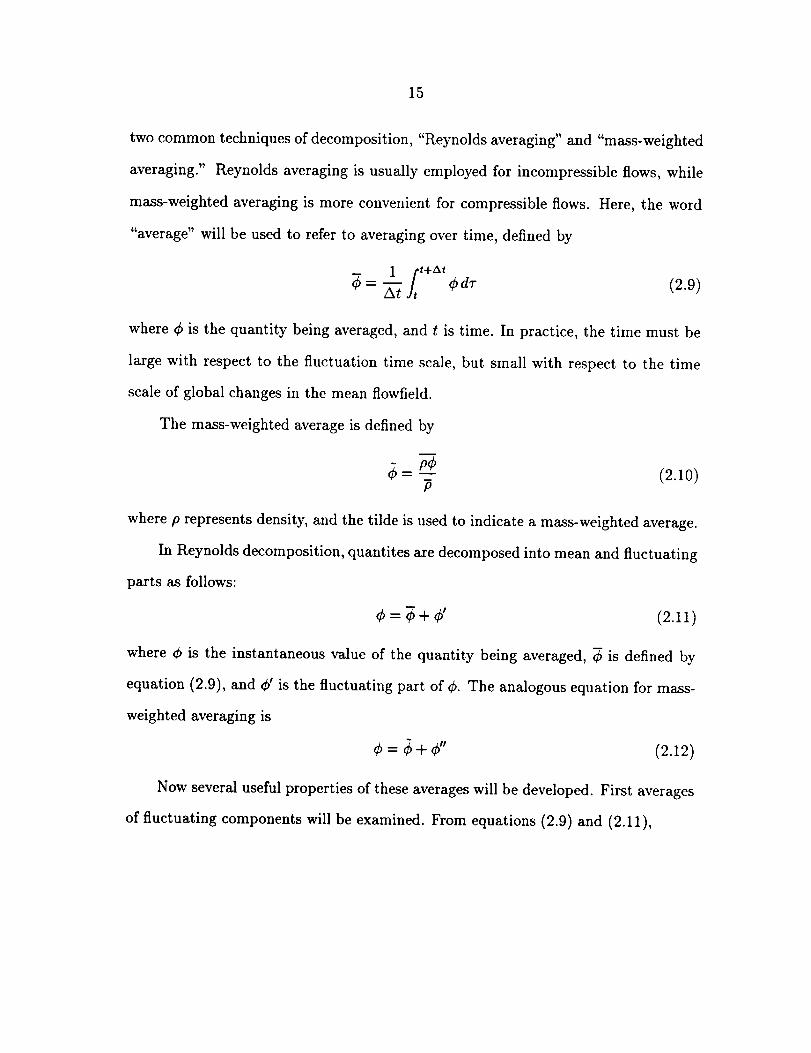
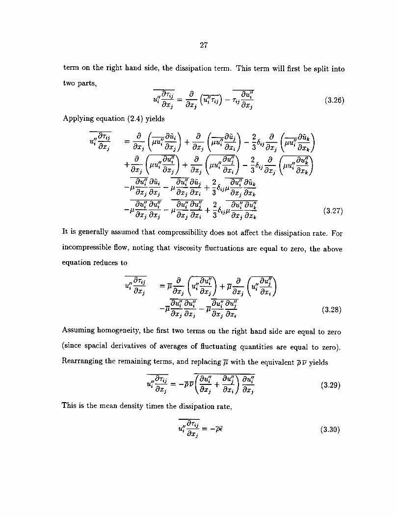
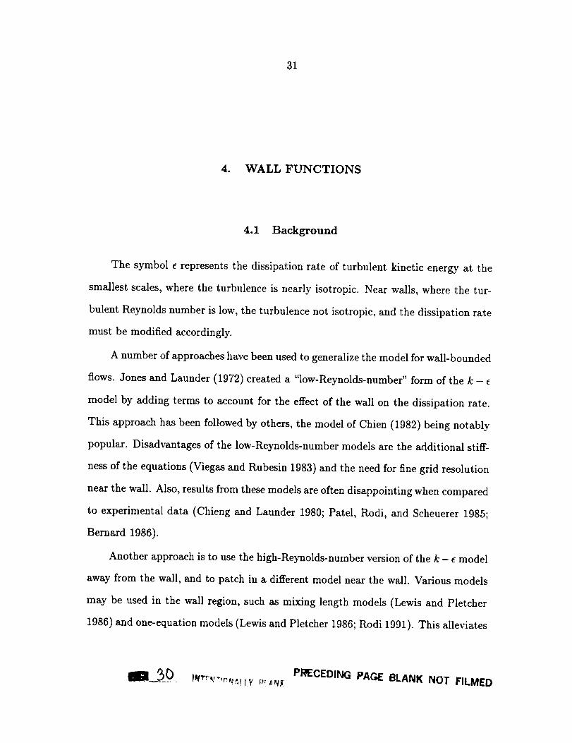
profile, similar to that shown in Anderson, Tannehill, and Pletcher (1984), is shown

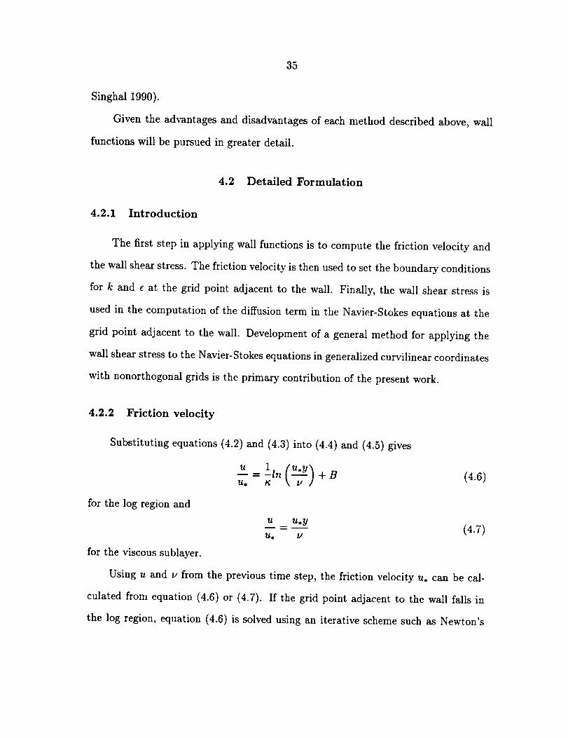
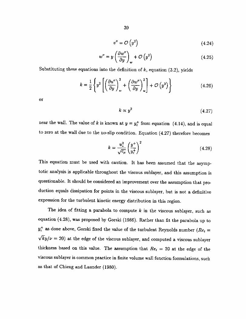
in Figure 4.1. The equation which describes the velocity profile in the log region is

u+ = l-In(y+)+ B (4.4)

33

÷

3O

25

2O

15

10

5

0

velocity profile..... equation (4.5)..... equation (4.4) i

. inner .i

_ v scous_. /->?" i ou!,r.sublayer i -_ 109 - region -

: region ---"/.. buffer ,_

region

100 101 102 103y+

Figure 4.1" Typical turbulent boundary layer velocity profile

where _ is the von Karman constant and B is an additional constant. Values of

and B have been empirically determined to fall in the ranges 0.40-0.41 and 4.9-5.5

respectively (Cebeci and Smith 1974). In the computations in the present study, the

values of 0.41 and 5.0 are used for K and B. These values were not chosen through

tuning of results, but simply because they are a frequently chosen pair, and are, in

the words of Coles and Hirst (1969), "satisfactory and non-controversial." In the

viscous sublayer,

u + = y+ (4.5)

The equations describing the velocity profile in the inner region are collectively called

the "law of the wall."

Knowledge of the structure shown in Figure 4.1 may be applied in such a way

that the entire boundary layer need not be resolved numerically. The grid point

34

adjacent to the wall may be placed well away from the wall, and the shear stress

inferred from the velocity at that point.

The use of wall functions has several advantages. The other techniques men-

tioned above require that the entire boundary layer be resolved. The grid point

adjacent to the wall must therefore be located in the viscous sublayer, typically at

a y+ of less than five. For wall functions, the first grid point is normally located in

the lower part of the log region, at a y+ of approximately 40 to 100. Given that the

rate at which the grid may stretch away from the wall is limited by most numerical

solution schemes, wall functions result in a large saving in the number of grid points

and the amount of computer memory required. Viegas and Rubesin (1983) found

that approximately half as many grid points were required when using wall functions

as compared to low-Reynolds-number models. Since the minimum grid spacing is

much larger for the wall function case, a larger time step may be used for a given

Courant number (for steady state computations), resulting in further saving in CPU

time. The reduced memory and CPU required when using wall functions can be

extremely important for the computation of complex three-dimensional flowfields.

One disadvantage of wall functions is that the log equation is not accurate for

some flowfields, such as those with regions of separated flow. Also, the standard wall

function formulation requires the assumption that the turbulence is in equilibrium

at the first grid point away from the wall, which is not always the case. Even with

these limitations, wall functions have been shown to yield results comparable, and

often superior, to those obtained with low-Reynolds-number models, including com-

putations of some complex flowfields (Chieng and Launder 1980; Viegas and Rubesin

1983; Viegas, Rubesin, and Horstman 1985; Chen and Patel 1987; Avva, Smith, and

35

SinghaJ 1990).

Given the advantages and disadvantages of each method described above, wall

functions will be pursued in greater detail.

4.2 Detailed Formulation

4.2.1 Introduction

The first step in applying wall functions is to compute the friction velocity and

the wall shear stress. The friction velocity is then used to set the boundary conditions

for k and e at the grid point adjacent to the wall. Finally, the wall shear stress is

used in the computation of the diffusion term in the Navier-Stokes equations at the

grid point adjacent to the wall. Development of a general method for applying the

wall shear stress to the Navier-Stokes equations in generalized curvilinear coordinates

with nonorthogonal grids is the primary contribution of the present work.

4.2.2 Friction velocity

Substituting equations (4.2) and (4.3) into (4.4) and (4.5) gives

for the log region and

(4.6)

U u.,y-- = _ (4.7)U, V

for the viscous sublayer.

Using u and u from the previous time step, the friction velocity u. can be cal-

culated from equation (4.6) or (4.7). If the grid point adjacent to the wall falls in

the log region, equation (4.6) is solved using an iterative scheme such as Newton's

36

method. If the point falls in the viscous sublayer, u, is calculated directly from

equation (4.7). The appropriate equation is determined as follows. Referring to

Figure 4.1, equations (4.7) and (4.6) may be seen to intersect at a single value of y+,

which will be called y+. Neglecting the buffer region as is often done for engineering

calculations (Tennekes and Lumley 1972), y+ delimits the viscous sublayer and the

log region. From equations (4.5) and (4.4),

y+ = 1In(y+) ..b B (4.8)

This equation is solved for y+ using Newton iteration. It is temporarily assumed that

the point in question is in the viscous sublayer. Using the velocity and viscosity from

the previous time step, equation (4.7) is solved for u., and y+ is calculated from

equation (4.3). If y+ is less than y+, the assumption that the point is in the viscous

sublayer was correct. Otherwise, the point is actually in the log region, and u. must

be recomputed using equation (4.6). The wall shear stress may then be computed

from equation (4.1).

4.2.3 Boundary conditions for k and

The values of k and e require some special attention near the wall. Both quanti-

ties vary rapidly near the wall, and this region of the flowfield is not resolved due to

the relatively coarse grid spacing. If k and _ can be estimated at the grid point ad-

jacent to the wall, these values may serve as boundary conditions for the turbulence

transport equations, and these equations do not have to be integrated all the way to

the wall.

For points in the log region, production and dissipation of turbulent kinetic

37

energyare approximately equal,

P = pc (4.9)

For a simple two-dimensional boundary layer, letting the y direction be normal to

the wall, the production term may be written

,, , du

P = -pu v' -_y (4.10)

or

du

P=Tt-_y

Combining equations (4.11) and (4.11 ),

du

(4.11)

From equation (4.6),

7"tdu= --- (4.15)

p dy

du u._ (4.16)

dy gy

rearranged,

_'t_yy = Pe (4.12)

From equations (3.1) and (3.6), the turbulent shear stress may be expressed as

du

Tt : Pt "_y

k 2 du

= c_p--e-- dy (4.13)

Solving this equation for e, substituting the result into equation (4.12), and applying

the definition of friction velocity (4.1) gives the desired expression for the equilibrium

turbulent kinetic energy,2

k= u. (4.14)

To arrive at an expression for the equilibrium e, equation (4.12) will first be

38

Substituting equation (4.16) and the definition of friction velocity (4.1) into equa-

tion (4.15)yields the final result3

?2,

= -- (4.1_)

If the grid point adjacent to the wall was found to be in the viscous sublayer,

the assumption that production equals dissipation is not valid. A different method

must therefore be employed to calculate k and e boundary conditions. The near-wall

behavior of k may be examined by expanding fluctuating velocity components in

Taylor series normal to the wall (e.g., Launder 1984). Taking the y direction to be

normal to the wall,

= uw + Y \ Oy ]w + O (y2) (4.18)

,,= vw + Y _, i)y ]_, + O (y2) (4.19)

,,W II

=ww+ y_ oy ]o + o G_) (4.20)

where the w subscript refers to the value at the wall. From the no-slip condition,

II II II 0Uw -- yw _- W w -- (4.21)

Very close to the wall, the flow may be considered incompressible for moderate

freestream velocities. From the incompressible continuity equation,

oy ] _ = 0 (4.22)

since (Ou"/Ox)_ and (Ow"/Oz),,, are equal to zero from the no-slip condition. Sub-

stituting equations (4.21) and (4.22)into (4.18)-(4.20),

u" = y \ Oy ]. + O (y2) (4.23)

39

v" = O (y2) (4.24)

w" -- y \ Oy ,]w -t- O (y2) (4.25)

Substituting these equations into the definition of k, equation (3.2), yields

k = _ y2L_, Oy ]w + _, Oy ],_] + 0 (y3) (4.26)

or

k o¢ y2 (4.27)

near the wall. The value of k is known at y = y+ from equation (4.14), and is equal

to zero at the wall due to the no-slip condition. Equation (4.27) therefore becomes

k- u._.__. (4.28)- fe; \y+)

This equation must be used with caution. It has been assumed that the asymp-

totic analysis is applicable throughout the viscous sublayer, and this assumption is

questionable. It should be considered an improvement over the assumption that pro-

duction equals dissipation for points in the viscous sublayer, but is not a definitive

expression for the turbulent kinetic energy distribution in this region.

The idea of fitting a parabola to compute k in the viscous sublayer, such as

equation (4.28), was proposed by Gorski (1986). Rather than fit the parabola up to

y+ as done above, Gorski fixed the value of the turbulent Reynolds number (Ret --

q"ky/v --- 20) at the edge of the viscous sublayer, and computed a viscous sublayer

thickness based on this value. The assumption that Ret = 20 at the edge of the

viscous sublayer is common practice in finite volume wall function formulations, such

as that of Chieng and Launder (1980).

4O

An expressionfor e is still needed for points in the viscous sublayer. Following

Rodi (1991), the length scale equation of Norris and Reynolds (1975) will be used,

where

l_ = cly (4.29)1 + 5.3/Ret

ct = _c_ 3/4 (4.30)

Now that k and l, are known, e is simply

k3/2e = _ (4.31)

In summary, if the point adjacent to the wall is in the log region, k and e are

computed from equations (4.14) and (4.17). If it is in the viscous sublayer, k and e

are computed from equations (4.28) and (4.31).

4.2.4 Application of rw to the Navier-Stokes equations

Having computed the friction velocity from equation (4.6) or (4.7), the wall shear

stress can be computed from equation (4.1) using the density from the previous time

step. The remaining task is to substitute the wall shear stress into the momentum

and energy equations.

The law of the wall was originally developed for two-dimensional boundary layers.

For three-dimensional boundary layers, if the boundary layer is not highly skewed,

the wall shear stress calculated above may be divided vectorially into components in

the two coordinate directions parallel to the wall, proportional to the velocity compo-

nents. If the boundary layer is skewed, a method of approximating the components

at the wall, such as extrapolating the velocities, could be employed. Skewness will

not be considered in the following development.

41

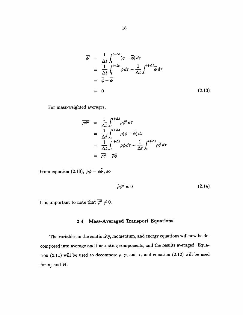
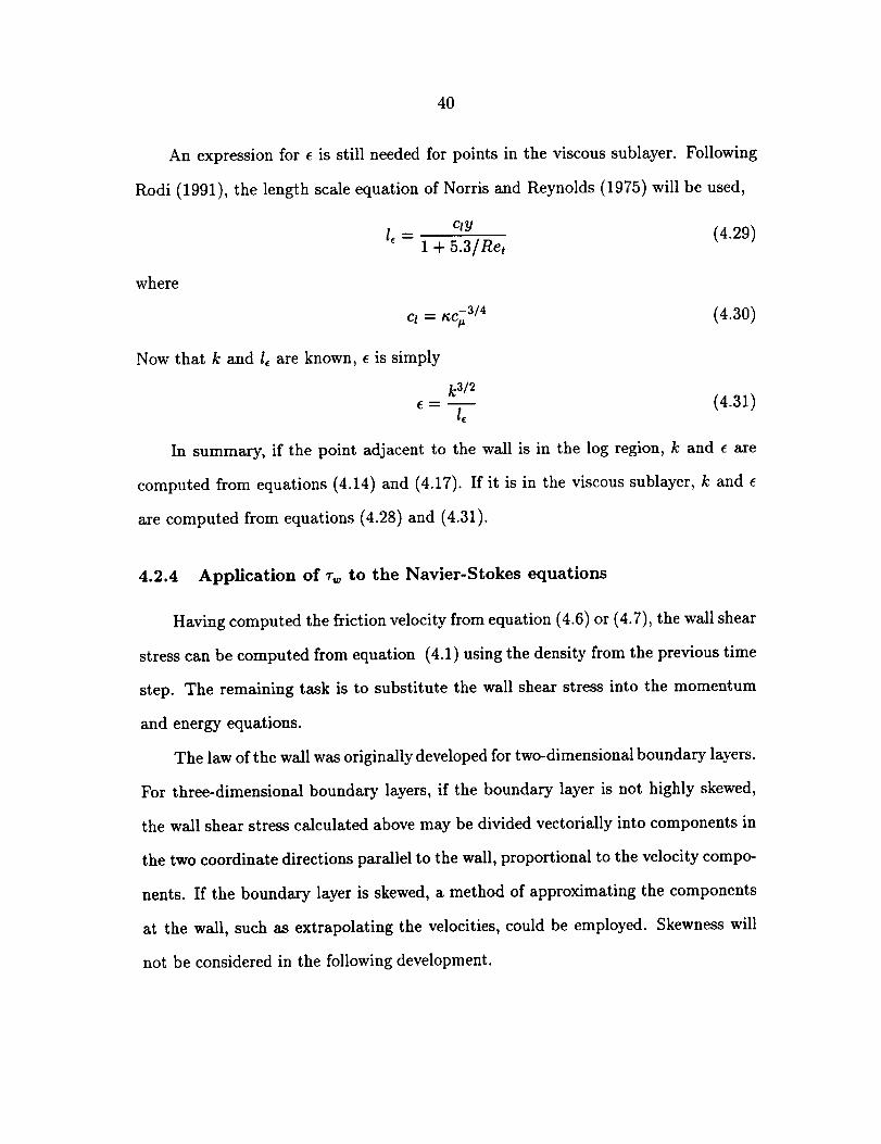
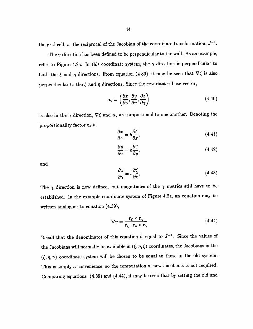
(a) (b) (c)

Figure 4.2: Definition of 7 coordinate direction

For generalized curvilinear coordinates, the application of the shear stress de-

duced from the law of the wall to the momentum and energy equations becomes

rather complicated. This is due to the fact that the shear stress components in the

cartesian coordinate system do not necessarily act parallel to the walls. Another

difficulty is encountered when there is no grid line perpendicular to the wall (i.e. the

grid is skewed at the wall). The shear stress calculated from the law of the wall

acts parallel to the wall, in a plane perpendicular to the wall, but this plane is not

necessarily defined by coordinate directions. A new coordinate direction, called "7,"

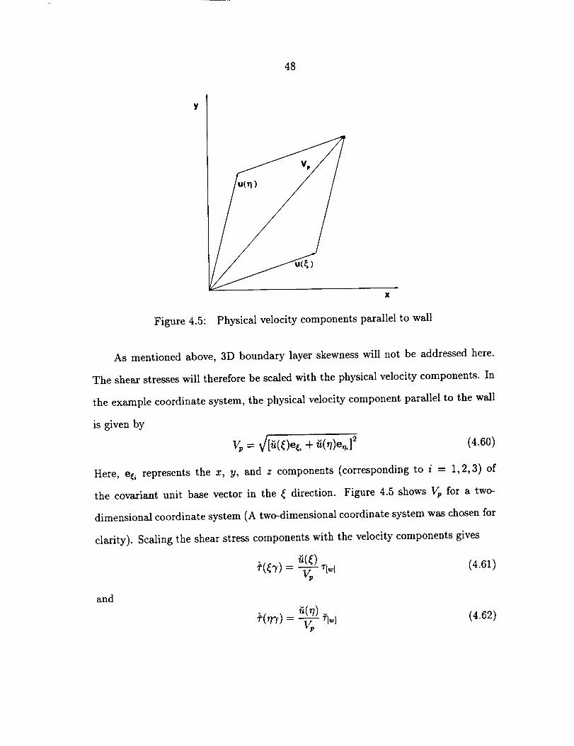
is defined to be perpendicular to the wall. This is shown in Figure 4.2 for the three

possible coordinate orientations.

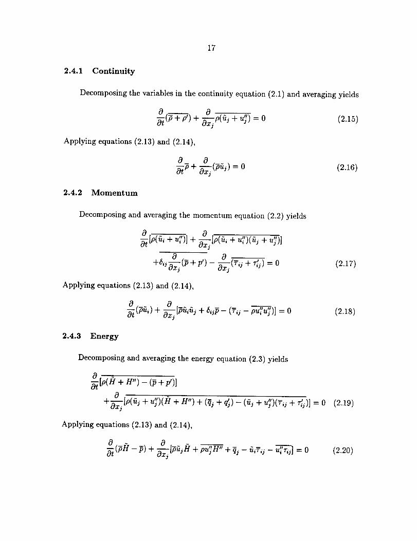
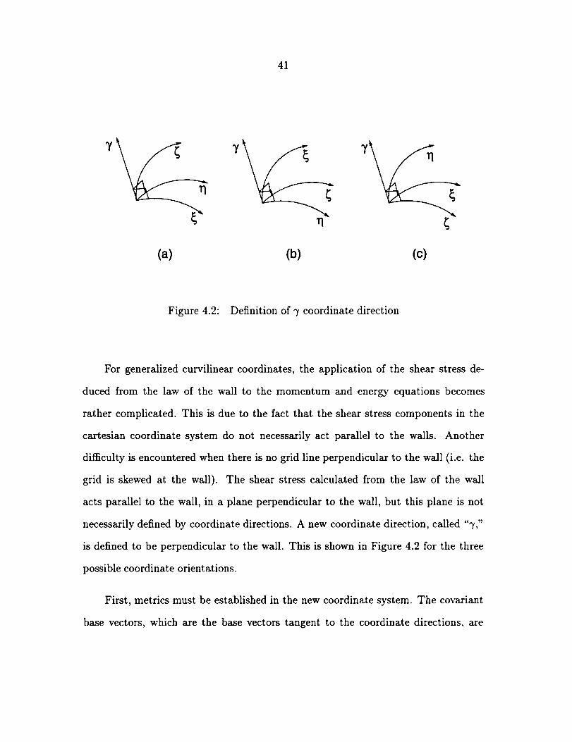
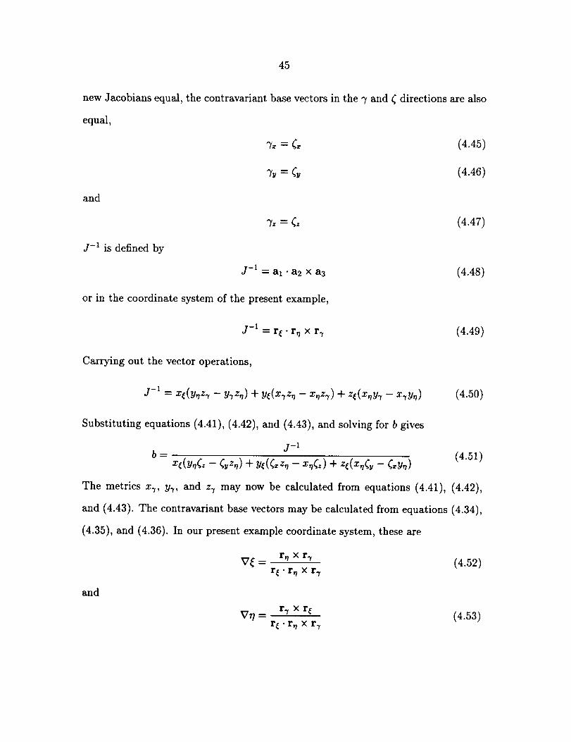
First, metrics must be established in the new coordinate system. The covariant

base vectors, which are the base vectors tangent to the coordinate directions, are

42

a 2

Figure 4.3: Covariant base vectors

given by

Orai = B (4.32)

where r is a position vector. These are shown in Figure 4.3. al represents the base

vector with components o_ o_ and o_ with similar definitions for the other two

coordinate directions. Unit covariant base vectors will also be needed, and are given

by

ai

ei = _ (no _-'_) (4.33)i

The contravariant base vectors are defined by (e.g., Sokolnikoff 1964)

al : a2 × a3 (4.34)al •a2 × a3

a2 _ it3 × al (4.35)a 1 • a 2 X a 3

43

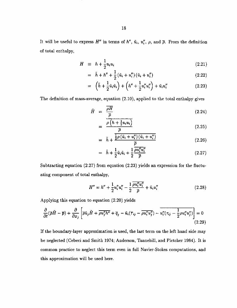
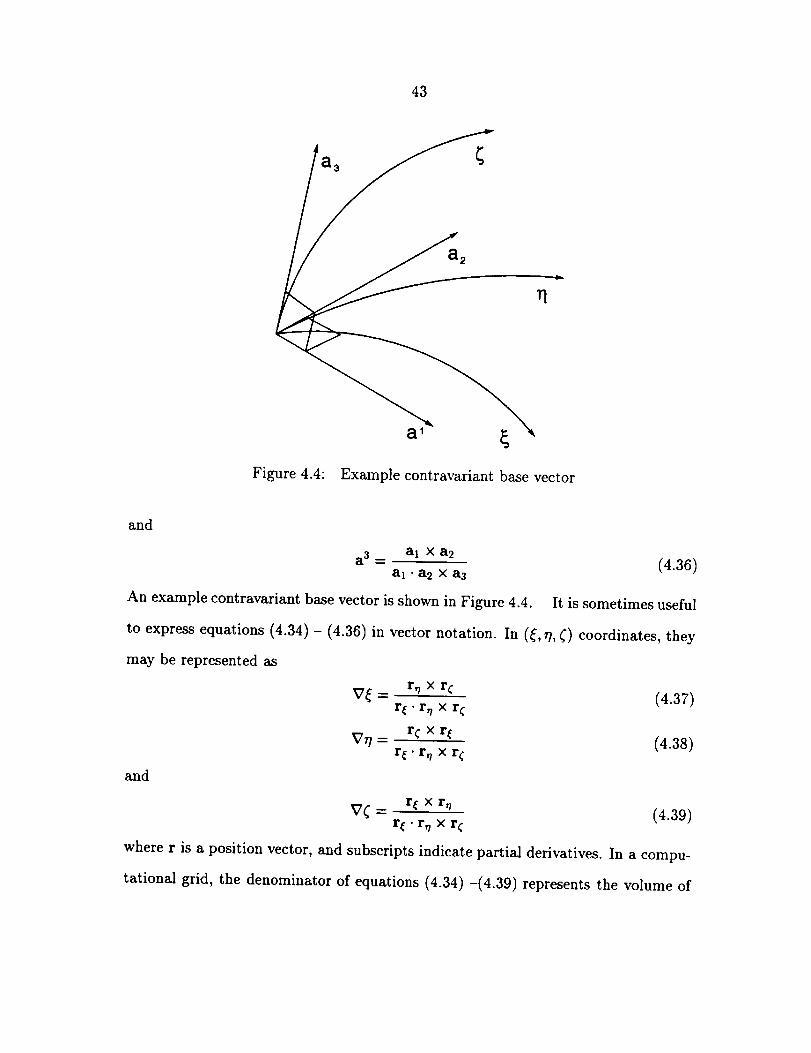
a 3

a 2

Figure 4.4: Example contravariant base vector

and

a3 = al x a2 (4.36)al " a2 × a3

An example contravariant base vector is shown in Figure 4.4. It is sometimes useful

to express equations (4.34) - (4.36) in vector notation. In (_, _/, _) coordinates, they

may be represented as

and

V_'- r, x re (4.37)r_ .r_ × re

Vr/= re x r_ (4.38)r_ • r_ x re

V_ = r,, x r_ (4.39)r_ -r_ x re

where r is a position vector, and subscripts indicate partial derivatives. In a compu-

tational grid, the denominator of equations (4.34) -(4.39) represents the volume of

44

the grid cell, or the reciprocalof the Jacobianof the coordinatetransformation, j-1.

The 7 direction has been defined to be perpendicular to the wall. As an example,

refer to Figure 4.2a. In this coordinate system, the 3' direction is perpendicular to

both the _ and 77directions. From equation (4.39), it may be seen that V( is also

perpendicular to the _ and r/directions. Since the covariant 3' base vector,

oy Oz)av = _,c93' c9-y'_ (4.40)

is also in the 3' direction, V_ and a_ are proportional to one another. Denoting the

proportionality factor as b,

and

Ox OC (4.41)N=b x ,

Oy 0¢=b--, (4.42)

Oz 0¢ (4.43)

written analogous to equation (4.39),

V3"-- r_ x r, (4.44)r_.r_ × r_

Recall that the denominator of this equation is equal to j-1.

the Jacobians will normally be available in (_, r/, _) coordinates, the Jacobians in the

(_, _?,3') coordinate system will be chosen to be equal to those in the old system.

This is simply a convenience, so the computation of new Jacobians is not required.

Comparing equations (4.39) and (4.44), it may be seen that by setting the old and

Since the values of

The 3' direction is now defined, but magnitudes of the 3' metrics still have to be

established. In the example coordinate system of Figure 4.2a, an equation may be

45

new Jacobiansequal,the contravariantbasevectors in the 7 and ( directions arealso

equal,

%=(x

and

j-1 is defined by

(4.45)

(4.46)

and

j-1 = al .a2 × a3 (4.48)

or in the coordinate system of the present example,

j-1 = r_.r, x r3 (4.49)

Carrying out the vector operations,

j-1 = x_(y,z._- _._z,,)+ y_(_:_z,- _,z_) + z_(_,y._- x._y,) (4.50)

Substituting equations (4.41), (4.42), and (4.43), and solving for b gives

j-1

b= x_(_,_z- ¢_z,) + y_(_xz,- x,5) + z_(x,¢_- _,,) (4.51)

The metrics x_, y3, and z3 may now be calculated from equations (4.41), (4.42),

and (4.43). The contravariant base vectors may be calculated from equations (4.34),

(4.35), and (4.36). In our present example coordinate system, these are

V_- r, x r_ (4.52)r_ • r_ x r_

Vrl = r_ x r_ (4.53)r_ • r_ x r_

,_z=¢_ (4.47)

46

The calculation of all the metric quantities that are needed for the coordinate trans-

formation is now complete.

Keep in mind that the whole idea of the present procedure is to replace the

shear stresses in the Navier-Stokes equations with those from the wall functions. For

finite difference schemes, this means that the shear stresses are required at a point

between the wall and the point adjacent to the wall (i.e. point 1½). In the absence of

a streamwise pressure gradient, the momentum equation evaluated at the wall shows

that the normal gradient of the shear stress is zero at the wall. This means that

the shear stress at point 11 is approximately the same as the shear stress at the

wall. For cases with streamwise pressure gradients, this is not the case. However,

it will be assumed here that the wall function shear stress is applicable at point 1½.

This is consistent with the use of the log equation (4.6), which technically is not

valid for flows with streamwise pressure gradients. It is common practice to use the

log equation for flows with moderate streamwise pressure gradients, since it gives

reasonable results for these cases (Launder 1984). Using the pressure gradient from

the previous time step, a better approximation for the shear stress at point 1½ could

be obtained from the momentum equation if desired.

The next step is to calculate the shear stresses in physical (x, y, z) coordinates

1 using the equation(e.g., r z_) at point 1_

+ -3'5 Joz ] (4.54)

These should be calculated in the same way that they are calculated in the discretized

Navier-Stokes equations, i.e. the same averaging procedure should be used to obtain

values at point 1½. The stresses are then transformed to the generalized coordinate

47

systemusing the standard tensor transformation

,_,_ 07`" 07 _ ;_Ox' OxJ

(e.g., Sokolnikoff 1964).

(4.55)

Here, the v symbol represents quantities in the generalized

the following equation (Aris 1962) is employed,

= J0-_ _Z,_`'7 (hOE) (4.56/

`',/3

where _(aj3) represents the physical components of the tensor. O_a is the metric

tensor,

Ox _ Ox _

g`'_ = 07`" 07 _

be needed:

o

where U`" represents the eontravariant velocity components,

_o 07" i-- -_x_U (4.59)

(4.57)

The physical velocity components in the generalized coordinate directions will also

(4.58)

Capital U is used for the contravariant velocity components and small u is used for the

physical velocity components in the physical coordinate directions to be consistent

with standard CFD notation.

coordinate system. For clarity, Greek letters are used for tensor indices in general-

ized coordinates, and Roman letters are used for physical coordinates. The tensor

x i represents the physical coordinate x, y, or z, and 3'`" represents the generalized

coordinate (, rh or 3'.

The stresses _`'a do not represent physical quantities. In order to obtain the

physical components of the shear stresses in the generalized coordinate directions,

48

y

Figure 4.5: Physical velocity components parallel to wall

As mentioned above, 3D boundary layer skewness will not be addressed here.

The shear stresses will therefore be scaled with the physical velocity components. In

the example coordinate system, the physical velocity component parallel to the wall

is given by

Vp = y/[fi(_)e¢, + _(r/)en,] 2 (4.60)

Here, e_ represents the x, y, and z components (corresponding to i = 1,2,3) of

the covariant unit base vector in the _ direction. Figure 4.5 shows Vp for a two-

dimensional coordinate system (A two-dimensional coordinate system was chosen for

clarity). Scaling the shear stress components with the velocity components gives

"_(_7) = _(_) (4.61)riw]

and

_(rrT) = _ T[w] (4.62)

49

where "_[wlis the wall shear stress from the wall functions. Brackets are used in

the notation of _[_] so that w is not confused with a tensor index. The symbol :

is used to indicate physical shear stress components which were deduced from the

wall function equations, as opposed to those computed from equation (4.56). The

physical shear stress tensor computed from equation (4.56) is now modified to reflect

the wall function values. In the present example, _(_7) and _(W/) calculated in

equation (4.56) are replaced by the values from equations (4.61) and (4.62).

The above procedure will now be reversed to transform the new physical stresses

in the generalized coordinate system to physical stresses in physical coordinates.

First, an equation is required to calculate tensor components from physical compo-

nents, i.e. the inverse of equation (4.56). It is convenient here to work in matrix

notation rather than with tensors. In order to express equation (4.56) in matrix

notation, matrices will be defined as follows:

P_._

r(ll) T(12) _'(13)

r(21) T(22) T(23)

T(31) V(32) _-(33)

(4.63)

T 11 T 12 T 13

T21 T 22 T 23

T31 T32 T 33

(4.64)

gll gl2 g13

g21 g22 g23

gal g32 g33

(4.65)

5O

S_

vY7 o oo vf_ o

o o gv_

(4.66)

The _ notation has been dropped, since these definitions hold for any coordinate

system. Noting that the matrix G is symmetric, equation (4.56) may be written in

matrix notation as

P = ST(S-1G) T (4.67)

Solving for T,

T-SI'[(S -' ( 0S)In the present example the new stress tensor may be computed from equation (4.68),

where P is

_'-- S-ll_[(S-ld)T] -1 (4.69)

P=

"_(11) "_(12) "_(13)

_(21) _(22) T(23)

"_(31) "_(32) "_(33)

(4.70)

Note that the stress components from equations (4.61) and (4.62) have been substi-

tuted into the 1_ matrix. Finally, returning to tensor notation (_ = _°#), the new

stress tensor must be transformed to physical coordinates,

_ij_ Ox i Ox j :_#r (4.71)

07':' 07 #

_.ij is the new shear stress tensor which is applied to the Navier-Stokes equations. A

summary of the procedure described above is shown in Table 4.1.

The application of the new stress tensor to the Navier-Stokes equations is straight-

forward. The central difference operator _¢ = ¢j+1/2 - ¢j-1/2 is typically used for the

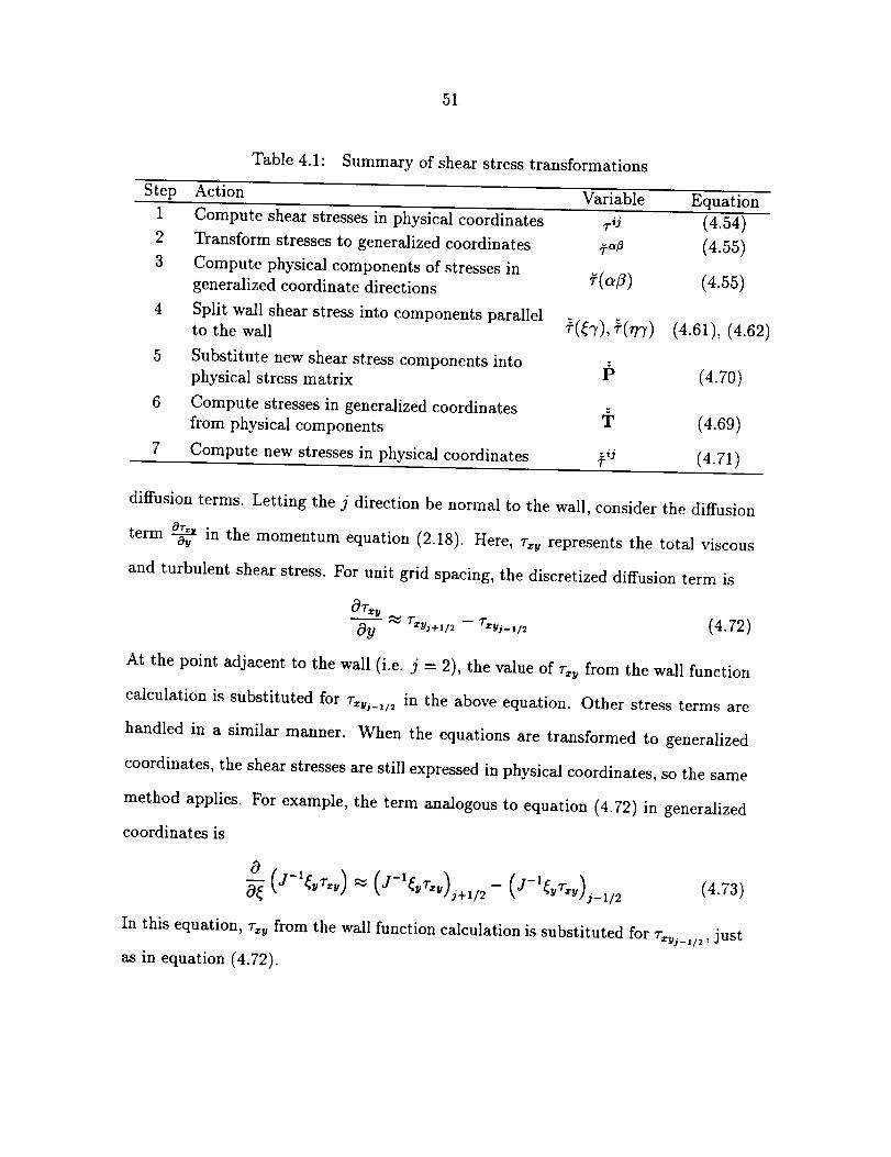
51

Table 4.1: Summary of shear stress transformations

Step Action Variable Equation

1

2

3

4

5

6

7

Compute shear stresses in physical coordinates TiJ

Transform stresses to generalized coordinates ._,_

Compute physical components of stresses ingeneralized coordinate directions "_(afl)

Split wall shear stress into components parallelto the wall

Substitute new shear stress components into

physical stress matrix P

Compute stresses in generalized coordinatesT

from physical components

Compute new stresses in physical coordinates _r_j

(4.54)(4.55)

(4.55)

(4.61), (4.62)

(4.70)

(4.69)

(4.71)

diffusion terms. Letting the j direction be normal to the wall, consider the diffusion

term o__ in the momentum equation (2.18). Here, 7"xyrepresents the total viscous0r

and turbulent shear stress. For unit grid spacing, the discretized diffusion term is

0T_-- _-, - (4.72)

cOy rxy_+,/_ Tz__,/2

At the point adjacent to the wall (i.e. j = 2), the value of r_ v from the wall function

calculation is substituted for v'_,_1/2 in the above equation. Other stress terms are

handled in a similar manner. When the equations are transformed to generalized

coordinates, the shear stresses are still expressed in physical coordinates, so the same

method applies. For example, the term analogous to equation (4.72) in generalized

coordinates is

cO(4.73)

In this equation, v_ v from the wall function calculation is substituted for r_v,_,/2,just

as in equation (4.72).

53

5. OTHER TURBULENCE MODELS

5.1 Introduction

In computing wall-bounded turbulent flows, there are many alternatives to the

k - e model with wall functions. Two common approaches are low-Reynolds-number

k - e models and algebraic models. It is therefore desirable to compare their perfor-

mance to the present wall function formulation. The low-Reynolds-number model of

Chien (1982) and the algebraic model of Baldwin and Lomax (1978) are quite popu-

lar and well-tested, and have therefore been chosen for comparison with the present

formulation.

5.2 Chien Low-Reynolds-Number Model

In the standard high-Reynolds-number k - e model, dissipation of turbulent

kinetic energy is assumed to occur at small scales where the turbulence is nearly

isotropic. This is reasonable for free shear flows, but is not the case in the vicinity

of walls. In low-Reynolds-number models, terms are typically added to the standard

k and e transport equations (Jones and Launder 1972; Chien 1982; Patel, Rodi, and

Scheuerer 1984; Mansour, Kim, and Moin 1989; Shih and Mansour 1990; Shih and

Hsu 1991; Michelassi and Shih 1991). The magnitudes of these additional terms drop

off rapidly away from the wall, resulting in the standard model.

PRECEDING PAGE BLANK NOT FILMED

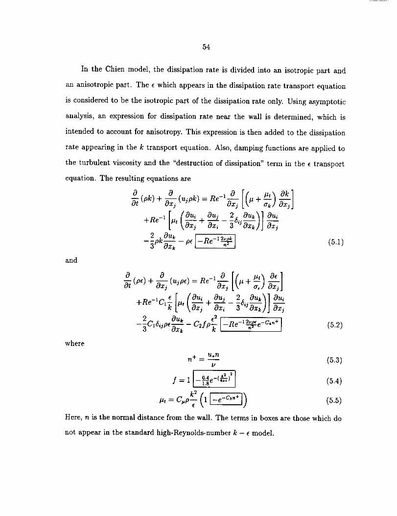
54

In the Chien model, the dissipation rate is divided into an isotropic part and

an anisotropic part. The e which appears in the dissipation rate transport equation

is considered to be the isotropic part of the dissipation rate only. Using asymptotic

analysis, an expression for dissipation rate near the wall is determined, which is

intended to account for anisotropy. This expression is then added to the dissipation

rate appearing in the k transport equation. Also, damping functions are applied to

the turbulent viscosity and the "destruction of dissipation" term in the e transport

equation. The resulting equations are

and

where

2 Ouk

\Ozj + Oz_ Oxj

2 kOUk I

-_ (p()+ _ (u_p_)= Re-1 # + _e 2 Ouk

2 Ou_ e2

(5.1)

(5.2)

n+ = u.n (5.3)V

= 0.4 -(k-L) _ If i-vAe .,, I (5.4)

k2 (1 I-e -c3"÷ l) (5.5)_, = c.p 7-

Here,n is the normal distance from the wall. The terms in boxes are those which do

not appear in the standard high-Reynolds-number k - e model.

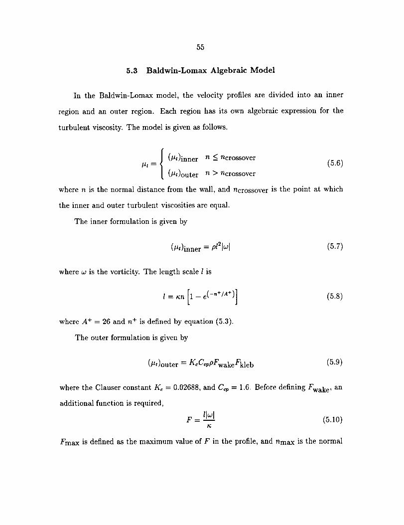
55

5.3 Baldwin-Lomax Algebraic Model

In the Baldwin-Lomax model, the velocity profiles are divided into an inner

region and an outer region. Each region has its own algebraic expression for the

turbulent viscosity. The model is given as follows.

! (#t)inner

L(Pt)outer

n _<ncrossover(5.6)

n > ncrossover

where n is the normal distance from the wall, and ncrossover is the point at which

the inner and outer turbulent viscosities are equal.

The inner formulation is given by

(#t)inner = Pl=lwl (5.7)

where ca is the vorticity. The length scale I is

l = t_n [1-e(-"+/a+)]

where A + = 26 and n + is defined by equation (5.3).

The outer formulation is given by

(5.8)

(#,)outer = KcC@PFwakeFkleb (5.9)

where the Clauser constant Kc = 0.02688, and Cq,

additional function is required,

= 1.6. Before defining Fwake, an

Fmax is defined as the maximum value of F in the profile, and nmax is the normal

F = llcal (5.10)t_

56

distance from the wall at which Fmax occurs. Fwake is given by

- minimum of / nmaxFmaxEvade (5.11)

[ n 2C, ok max(udi f) /Fmax

Udi f is the difference between the minimum and the maximum magnitude of velocity

in the profile, and C_k - 0.25.

Finally, Fkleb is the Klebanoff intermittancy factor,

where Ckleb = 0.3.

[ Ck,eb___ ]-1Fkleb= 1+55( _6• \ nmax /

(5.12)

57

6. NUMERICAL METHOD

6.1 Nondimensional Equations

For purposes of nondimensionalization, the following reference quantities are

used: velocity, aoo; density, p_; temperature, 7Too; length, Lref; time, Lref/a_¢;

and viscosity,/.t_. Using boldface type for dimensional quantities, variables in the

Navier-Stokes and k - e equations are nondimensionalized as follows:

_ u p _ ep= U_ a--_ p= e=po_aoo

h E- E H=H xh= _ p_= _ _=

t T r qt- L_el/ao_ T = _ z = _tooaoo/L_f q - I_o_a_2/L_ef

kk: _ _-- a 3/Lref

Applying these definitions to the continuity, momentum, and energy equations

(2.16), (2.18), and (2.34), and retaining average symbols only in terms containing

fluctuating quantities,

_p + (p._) = 0 (6.1)

(6.2)

0 0

_(E)+_-_xj{(E+p)uj+Re-'[q¢+Repu_'h"-u,(vij-Repuiuj)]}=0 (6.3)

58

wherethe Reynoldsnumber Re is defined by

and

Re - p_aooLre.f

Similarly, the turbulence transport equations (3.31) and (3.32) become

-_ (pk)+ -g-_(u_pk)= Re-' _,+ _

(6.4)

(6.5)

(p_)+ (_p,) =Re-'b-__ , +2 c3uk

_,Ox_ + Ox,_ Oxj

2 .,.., OU k (2

The nondimensional turbulent viscosity is given by

(6.6)

k 2

ut = Re %-- (6.7)(

6.2 Vector Form of Equations

The transport equations for conservation of mass, momentum, and energy are

usually written in vector form. Let x, y, and z be the three spatial coordinates and

u, v, and w the respective velocity components. The flux vectors are divided into

inviscid parts E, F, and G and viscous parts E,,, F,,, and Gv. Equations (6.1), (6.2),

and (6.3) may then be written

OQ OE OF

-_+Tz+N+---oc R_,(oF,o oF. oGo az k oz +--_y+ Oz] =0 (6.8)

59

where the dependent variable vector is

and the flux vectors are

pu

pu 2 + p

E = puv

puw

(E + p)u

Eli

F0

!T_

"ffxz

e_

F

Q _._

P

pu

pv

pw

E

(6.9)

pv

puv

pv 2 + P

pvw

(c + p)v

0

Fli= r_

ry_

f_

Vii --"

pw

puw

pvw

pw 2 + P

(c + p)w

0

T_z

r_z

rzz

g_

(6.10)

(6.11)

where, utilizing the Boussinesq approximation (equation (3.1)) and the model for tur-

bulent energy diffusion (equations (3.8) and (3.9)), and employing subscript notation

to indicate partial differentiation,

[4 2-r_ = (_,+ _,,) _,,. - _ (v_+ w_ )] 2- Re -_pk (6.12)

(6.13)

(6.14)

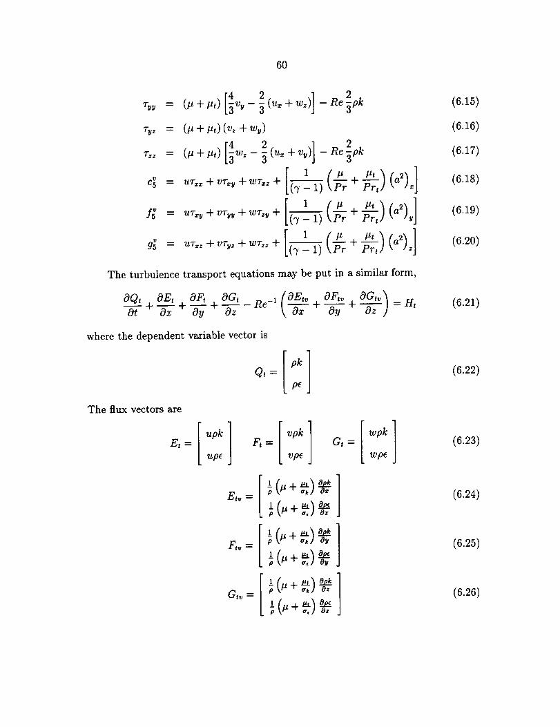
6O

7"yy

_z

"rzz

e_

9_

2 w_)] Re_pk= (, +,,) [3v_- 5(u_ + -

= (_ + _,)(v_ + w_)

[4 2 ] 2 k= (_ + _,) 5w_- _ (u_+ v,) - Re _p1

1 (.

1(.

The turbulence transport equations may be put in a similar form,

OQ,+OE, OFt OG, Re_,[OE,,, OFt,, OGt,,_"_x+'-ff'yy + O---z- \-"_-x +'-_y + Oz I-Hi


pkQt =

pe

The flux vectors are

E t

upk

upe

r_ "-"

vpk

vpe

wpkGt -

wpe

Etv

Ft_

etv

(6._5)

(6._6)

(6.17)

(6._8)

(6._9)

(6.20)

(6.21)

(6.22)

(6.23)

(6.24)

(6.25)

(6.26)

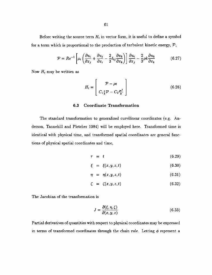
61

Beforewriting the sourceterm Ht in vector form, it is useful to define a symbol

for a term which is proportional to the production of turbulent kinetic energy, P,

= Re-' ,, + (6.27)

Now Ht may be written as

_p - pe(6.28)

6.3 Coordinate Transformation

The standard transformation to generalized curvilinear coordinates (e.g. An-

derson, Tannehill and Pletcher 1984) will be employed here. Transformed time is

identical with physical time, and transformed spatial coordinates are general func-

tions of physical spatial coordinates and time,

r = t (6.29)

= ((x,y,z,t) (6.30)

rl = rl(x,y,z,t) (6.31)

6, = _(z,y,z,t) (6.32)

The Jacobian of the transformation is

j = O(_,r/,_) (6.33)O(z, y, z)

Partial derivatives of quantities with respect to physical coordinates may be expressed

in terms of transformed coordinates through the chain rule. Letting ¢ represent a

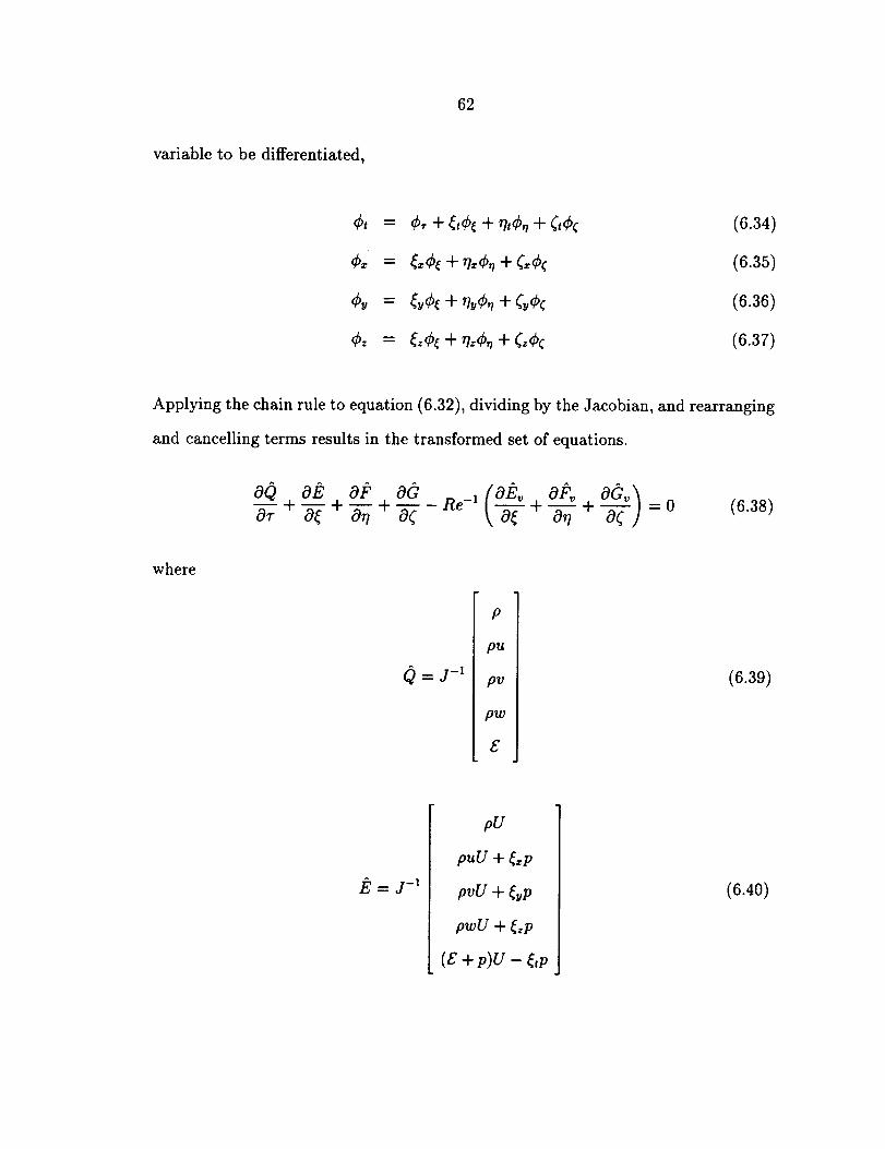
variable to be differentiated,

62

¢, -- ¢_ + _t¢_ + the, + _t¢¢ (6.34)

¢_ -- _¢_ + 7/z¢, + ¢_¢¢ (6.35)

¢_ = _y¢_ + _?v¢, + _¢¢ (6.36)

Cz = _z¢_ + r/_¢_ + _¢¢ (6.37)

Applying the chain rule to equation (6.32), dividing by the Jacobian, and rearranging

and cancelling terms results in the transformed set of equations.

0--_ + "-_ + _ + cO-'(- Re-1 \ 0_ + _ + --_-/ = 0 (6.38)

where

Q=j-1

P

pu

pv

pw

£

(6.39)

E=j-I

pU

puU + (_p

pvU + _p

pwU + _p

(e + p)V - _,p

(6.40)

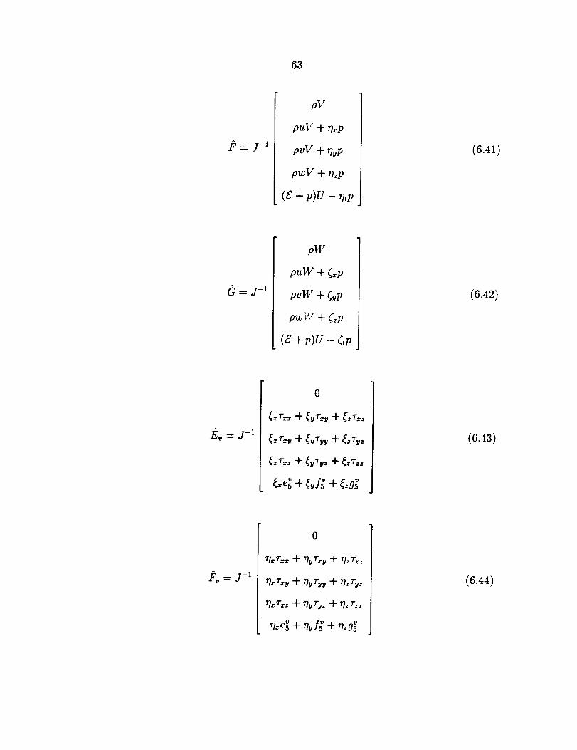
63

_=j-1

pV

puV + _7_p

pvV + _?_p

pwV + _zp

(8 + p)V - _tp

(6.41)

G__ j-i

pW

puW + _,p

pvW + _p

pwW + _zP

(E + p)u - ¢,p

(6.42)

/_ = j-1

0

(6.43)

0

_r._ + p.r_.+ _r w (6.44)

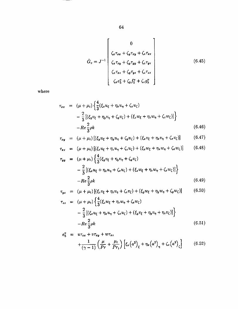
64

where

ev - j-1

0

4

- _[(_ + ,I,,_,+ ¢_v_)+ (_._+ _ + _;_)]2

-Re -_pk

r_ = (, + ,,)[(_u_ + '1_'_,+ ¢_u¢)+ (_,_ + ,7_v,+ ¢_v¢)]

r_ = (_ + _,) 5(_ + _, + ¢_¢)

2 k-Re -_p

: }2

-Re -_pk

e 5 ---- uv:=Wvv:yWWV=_

1

(6.45)

(6.46)

(6.47)

(6.48)

(6.49)

(6.50)

(6.5_)

(6.52)

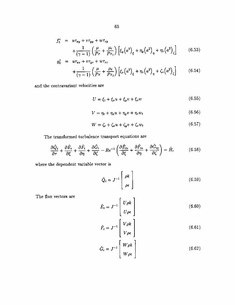
65

f_ - UT_y + Vryy + w'rz_

1

g_ = UTxz + VT_z + WVz_

1

and the contravariant velocities are

(6.53)

(6.54)

u = _ + _xu+ _v + _w (6.55)

V = rh + r/_u + rbv + rhwt

W = G+Gu+_v+Gw,

The transformed turbulence transport equations are


The flux vectors are

Et = j-1 Upk

U pe

._, j-1 V pk

Vpe

(6.56)

(6.57)

(6.58)

(6.59)

(6.60)

(6.61)

(6.62)

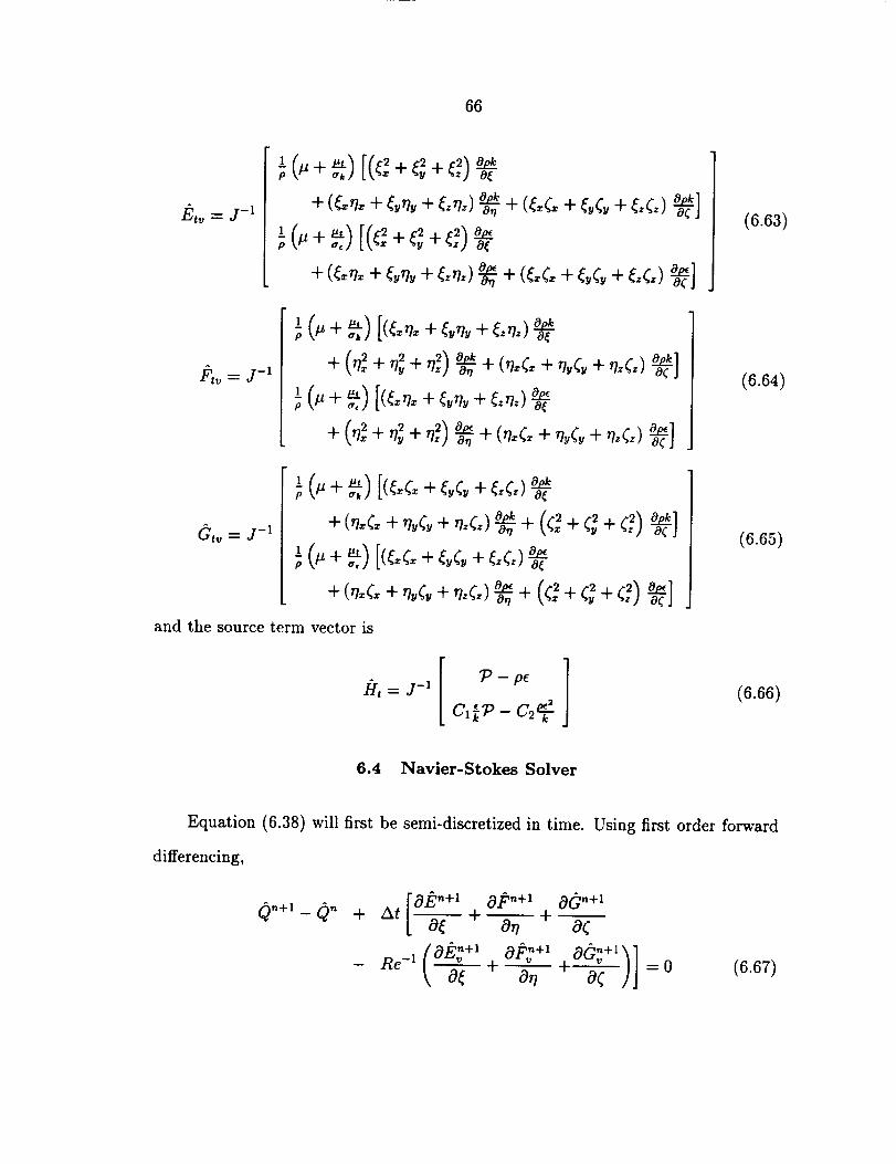
66

Etv "- j-i (6.63)

-_tv = j-1

Gtv -- j-1

and the source term vector is

(6.64)

(6.65)

/':/t -- j-17_ -- pc.

(6.66)

6.4 Navier-Stokes Solver

Equation (6.38) will first be semi-discretized in time. Using first order forward

differencing,

Qn+' -- On [a/_-+t op.+t Od,,+,+ at o--_+0---7-+ o---T-

(o_+' ob +' o_"+')]- Re-X _, O_ + Orl + Of =0(6.6?)

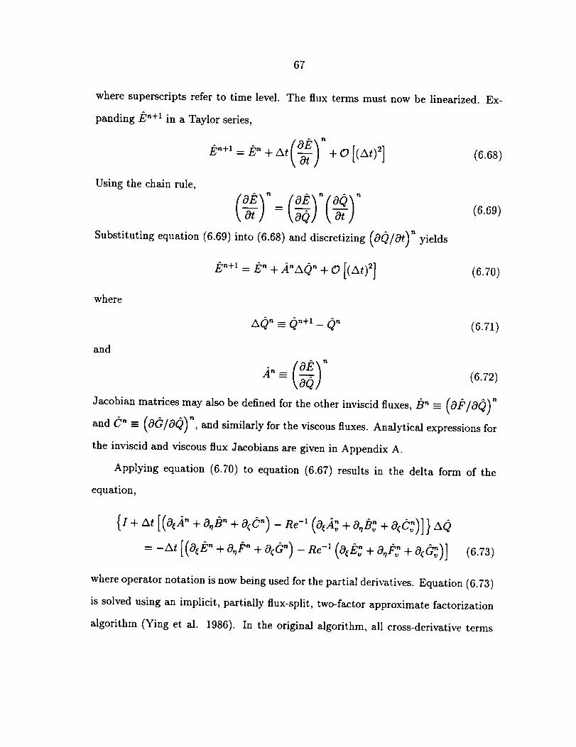
67

where superscripts refer to time level. The flux terms must now be linearized. Ex-

+o [(At)_] (6.68)

panding En-F1 in a Taylor series,

Using the chain rule,

Substituting equation (6.69)into (6.68) and discretizing (O(2/Ot)" yields

P,"+'= E"+ A"AO,"+ O[(,_n_]

_0" - ,O"+'- O"

\aq]

where

and

(6.70)

(6.71)

(6.72)

Jacobian matrices may also be defined for the other inviscid fluxes, #" - (o_/oQ)"

and C" - (0G/0(_)", and similarly for the viscous fluxes. Analytical expressions for

the inviscid and viscous flux Jacobians are given in Appendix A.

Applying equation (6.70) to equation (6.67) results in the delta form of the

equation,

{i +_,,[(a,,_-+a,bo+a,o.)- R.-,(a,._:+o,b:+a,e:)]}AO=-_, [(o,_o+o,p.+o,o°)- R_-,(o,E:+o_: +0,o:)] (_73/

where operator notation is now being used for the partial derivatives. Equation (6.73)

is solved using an implicit, partially flux-split, two-factor approximate factorization

algorithm (Ying et al. 1986). In the original algorithm, all cross-derivative terms

68

were neglected,and viscousterms wereretained only in the direction normal to the

wall (thin-layer assumption). Here, viscous terms are retained in all three directions,

with all cross-derivative terms neglected. In the flux-split direction (_), the viscous

terms cannot be linearized if a tri-diagonal solver is to be employed, so they are

included only on the right hand side.

The flux vector splitting method of Steger and Warming (1981) is used for con-

vection terms in the _ direction. The _ direction inviscid Jacobian A is therefore split

as follows,

= 4 + + e]- (6.74)

where

A + = 7_A+T -1 (6.75)

and

.4- = 7_/_-T -1 (6.76)

/k+ is a diagonal matrix containing the positive eigenvalues of Ai, and A- contains

the negative eigenvalues. The columns of T are the right eigenvectors of Ai.

Substituting difference operators, adding smoothing, and applying approximate

factorization to equation (6.73),

The difference operators are defined by

- Cj -

69

1

(6.78)

Similar definitions hold for the other two coordinate directions. Smoothing is required

for the central-differenced directions to ensure stability. The smoothing operators are

given by

where

T)exp¢ = j-1 e2_¢s¢/3_c; + e4_¢

(6.79)

(6.80)

I Ifp, (6.81)

e2 and e4 are the second and fourth order smoothing coefficients, and s¢ is the spectral

radius of the inviscid flux Jacobian matrix. The factor of 2.5 in the implicit smoothing

operator is included to ensure stability, given the fourth order explicit smoothing.

The ¢_function is designed to switch from fourth order to second order smoothing in

regions of rapid spatial variation in pressure, such as at a shock wave. The spectral

radius scaling is included to emulate the numerical dissipation inherent in upwind

difference schemes (Pulliam 1985). The r/ direction smoothing operators are similar

to equations (6.79) and (6.80), with all occurrences of the symbol ( replaced by rl.

6.5 k- e Solver

The k - e equations are solved uncoupled from the Navier-Stokes equations. The

linearized equations are simpler in form than the Navier-Stokes equations because

7O

they arecoupledonly through the source terms if the functional dependence of #t on

k and e is neglected in the viscous terms. Flux Jacobians for the convection terms

axe simply diagonal matrices containing the contravaxiant velocities. The linearized

equations in delta form axe

where

and

{I[1 + At(O_U -+-OnV + 0¢W)]

--At ./_e -1 [0_ (J-1,Af#IGQ_J) + 0rl (J-ldv'#4Gq_/J) + 0_" (J-ldv'_6(_'_J)]

oo

(6.82)

(6.83)

31 = _2 + _2 + _ (6.84)

2 (6.85)#, = ,7,_+ ,7,+ o_

#. = ¢,_+¢,_+¢_ (6.86)

An analytical expression for DT, the turbulent source term Jacobian, is given in

Appendix A.

Equation (6.82) is solved using a conventional three-factor approximate factor-

ization scheme with flux vector splitting and first-order differences for the convection

terms in all three directions. Central differences are used for all diffusion terms.

Several methods of handling the source terms are available. Here, they have been

placed in a single factor, since this method is both simple to implement and is also

71

computationally efficient (Shih and Chyu 1991). The resulting equation is

(6.87)

The _ and _ direction factors require solution of uncoupled equations, since there

is no source term Jacobian present. A specialized solver was therefore written for

banded tridiagonal matrices to enhance computation speed. In the _ direction, a

block solver is required due to the source terms. Since two-by-two blocks may be

inverted algebraically, a second specialized solver was written for the ( direction.

Details of both of these solvers are given in Appendix B.

An additional consideration in the solution of these equations is the possibility

of obtaining negative values for k and e. Negative values are physically impossible,

but are admitted by the modeled transport equations. Lower limiters are therefore

used for both equations. After each step, any values of pk or pe that are below the

specified limit are bumped up to that limit. The freestream values of pk and pe are

used for the limiters, since the physical (as opposed to numerical) values are not

expected to fall below those in the freestream. One run was started from scratch (all

dependent variables set to freestream values) with the limiters turned off, and it was

unstable. Addition of the limiters solved the problem. After the solution had partly

converged, the limiters were again turned off, and the solution remained stable. The

72

starting transient had caused the unphysical values in the first case, and once the

solution settled down, the limiters were unnecessary.

73

7. RESULTS

7.1 Introduction

A formulation designed for general geometries and skewed grids must also work

on simple geometries and orthogonal grids. The ubiquitous fiat plate has therefore

been chosen for the first set of test cases. First, turbulent flow over a semi-infinite

flate plate was computed on an orthogonal grid. The next step was to verify that the

formulation is effective when the grid is skewed at the wall, so the same flat plate

was solved with a skewed grid.

The tensor transformations in the present formulation contain functions of all

of the metrics. When any of the generalized coordinate directions are orthogonal to

physical coordinate directions, some of the metrics will be identically equal to zero.

One final fiat plate test case was run with the entire domain at a thirty degree angle

with the physical coordinate system (at zero angle of attack) to bring additional

metrics into play and further test the method.

One additional flat plate test case was run to verify the coding of the Chien

(1982) low-Reynolds-number model.

After having verified the present formulation for flat surfaces, the next step

was to solve a well-behaved (non-separated) flow over a curved surface. Ramaprian,

Patel, and Choi (1978, 1980) took measurements of the turbulent flowfield around a

74

body of revolution at both zero and fifteen degree angles of attack. The zero degree

(axisymmetric) flowfield was computed using the present wall function formulation as

well as the Chien (1982) low-Reynolds-number model and the Baldwin-Lomax (1978)

algebraic model, and the results compared to the measurements. Each computation

was carried out using grids with three different wall spacings to determine the grid

sensitivity of each model.

Finally, the present wall function formulation was tested on a complex three-

dimensional flowfield. Separated flow over a prolate spheriod at ten degrees angle

of attack was computed, and the results compared to the measurements of Kreplin,

Vollmers, and Meier (1982).

7.2 Flat plate

The first test case is the computation of incompressible, turbulent flow over a

semi-infinite flat plate with zero pressure gradient. The freestream Mach number

was set to 0.2 to minimize compressibility effects without getting too close to the

incompressible limit of the solver. The Reynolds number based on freestream velocity

was 1 x 106 at the upstream boundary, and 8 x 106 at the outflow boundary. The

reference length was defined such that the distance from the virtual origin of the

boundary layer to the upstream boundary was one unit of length. All lengths were

normalized by this distance.

The streamwise and normal coordinate directions are x and z in physical coor-

dinates and _? and _ in transformed coordinates. Wall functions are expected to give

the most accurate results when the grid point adjacent to the wall falls in the log

region. The distance from the wall to the grid point adjacent to the wall, which will

75

be referredto asthe "wall spacing,"waschosento equal0.0035(nondimensionalized

by the referencelength describedabove)so that Az + _-, 140, which is well into the

log region. Az + is the wall spacing in wall coordinates. The domain extended from 1

to 8 in the streamwise direction, and 0 to 1.5 in the normal direction. The location of

the outer edge was chosen to exceed ten times the estimated boundary layer thickness

at the downstream boundary. The 101 x 61 (streamwise x normal) orthogonal grid

is shown in Figure 7.1.

An upstream streamwise velocity profile was specified using the law of the wake

(Coles 1956),

where

u + = lln(y+) + B + (7.1)

II is a function of the streamwise pressure gradient, and is approximately equal to

The boundary layer thickness, 6, was estimated0.5 for pressure gradients of zero.

from the equation (White 1974)

- _ 0.37Re-_ 1/5 (7.3)x

At the inflow boundary, the normal velocity component was set to zero, the den-

sity was fixed at the freestream value, and the pressures were set by extrapolation

(P,7=1 = P,7=2). At the outflow boundary, pressure was fixed at the freestream value,

and density and both components of momentum were extrapolated. At the outer

edge, density, both components of momentum, and pressure were extrapolated. At

the wall, velocities were set to zero, and density and pressure were extrapolated.

The upstream turbulence quantities were more difficult to estimate. A detailed

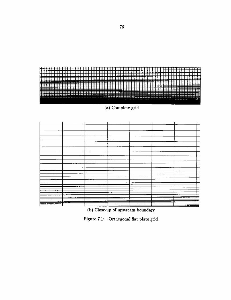
76

(a) Completegrid

(b) Close-upof upstream boundary

Figure 7.1: Orthogonal flat plate grid

77

turbulent kinetic energy profile was measured for incompressible flow over a fiat

plate with zero streamwise pressure gradient by Klebanoff (1955), but at a Reynolds

number of 4.2 x 106. These data were used to estimate the distribution at the present

Re = 1 x 106.

The friction coefficient was first calculated using the equation (White 1974)

O.455

C; ,_ in 2 (0.06ne_) (7.4)

Combining the definition of friction velocity, equation (4.1), and the definition of

friction coefficient,

(7.5)1 2_P_U_o

the friction velocity can be expressed as a function of friction coefficient,

u. = 2P_u_°Ct (7.6)pw

Since the grid spacing at the wall was chosen such that the first grid point away from

the wall was in the log region, k at that point was calculated from equation (4.14).

The next step was to interpolate the Klebanoff k distribution onto the present

grid using a cubic spline (Hornbeck 1975). As was expected, the value of k at the point

adjacent to the wall did not match the value calculated from equation (4.14). The

whole k distribution was multiplied by the ratio of the two values to force the correct

value at the given point. Finally, freestream values were cut off at k/U_ -- 0.0002,

Klebanoff's approximate freestream k.

The upstream e distribution was estimated using a method described by Launder

et al. (1972). The ratio of turbulent shear stress to turbulent kinetic energy was

estimated to equal the constant 0.3. Since the k distribution was estimated above,

78

the turbulent shear stress distribution was also "known." Finally, the e distribution

was computed from equation (4.13).

At the outflow boundary and the outer edge, k and e were extrapolated. Values

of k or e are not required at the wall when using wall functions.

The friction velocity was computed at each point along the plate from either

equation (4.6) or (4.7). Since the friction coefficient is easily deduced from the fric-

tion velocity, comparison with experimental friction coefficients is a good check on

the effectiveness of a wall function formulation. The friction coefficient distribution

for incompressible turbulent flow over a flat plate with zero pressure gradient is well

established. An accurate and well-tested equation for the friction coefficient distri-

bution is given by (White 1974)

Re,= _' + 7 ez(z2- 4z+6)- 6- 2z 12 _ (7.7)

where

and

= _ (z.s)

Z=tcA

The computed results are within 1½% of the values from the equation.

(7.9)

The

Thecomputed friction coefficients are compared with equation (7.7) in Figure 7.2.

computed results are within 1½% of the values from the equation.

A sample velocity profile is compared with test data in Figure 7.3, where/_ is the

boundary layer thickness and Uinf is the freestream velocity. The measurements were

taken by Klebanoff (1955) at a Reynolds number of 4.2 x 10 6 based on freestream

velocity and distance from the virtual origin of the plate. The computed profile

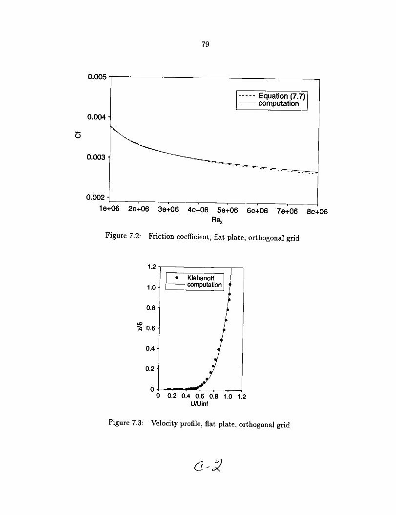
79

0.005

0.004

0.003

0.002

..... Equation (7.7)-- computation

1e+06i | | w i

2e+06 3e+06 4e+06 5e+06 6e+06 7e+06

R_

Figure 7.2: Friction coefficient, flat plate, orthogonal grid

8e+06

1.2

1.0

0.8

¢,o;_ 0.6

0.4

0.2

00

. K'eOan° I!computation

=l W

0:2 0.4 0:8 0:e 1:o1.:U/Uinf

Figure 7.3: Velocity profile, flat plate, orthogonal grid

8O

is at the sameReynoldsnumber assumingthat the virtual origin is at x - 0. The

boundary layer thickness for the test data was taken to equal the "nominal thickness"

of three inches quoted in Klebanoff's paper. For the computation, the boundary layer

thickness was taken at the point at which the velocity reached 99% of the freestream

velocity.

At the grid point adjacent to the wall, the computed velocity is slightly higher

than the test data. Since this grid point falls in the log region, the computed friction

coefficient must also be larger than the value corresponding to the test data. It

would be more accurate to compare velocity profiles at the same momentum thickness

Reynolds number rather than Reynolds number based on distance from the virtual

origin of the plate, since it is difficult to locate the virtual origin precisely. For the

present computation, however, it is also difficult to compute the momentum thickness

accurately due to the coarse grid spacing at the wall. Since the boundary layer is not

resolved near the wall, the numerical integration required to compute the momentum

thickness would also be inaccurate.

7.2.1 Skewed grid

In the present wall function formulation, a new coordinate direction is defined

normal to the wall, and physical shear stresses are computed using this new direction.

A simple test case with a grid that is nonorthogonal at the wall was desired to check

this part of the procedure. A case similar to that computed above was chosen,

but using a grid which is skewed near the wall. The grid lines parallel to the plate

(constant _) are identical to those in the orthogonal grid. The grid is orthogonal to the

plate at the upstream boundary. Moving downstream, the grid lines gradually become

81

more and more skewed, until they reach an angle of sixty degrees with respect to the

plate. They then remain at this angle for the rest of the domain. This configuration

was chosen for two reasons. First, the upstream boundary definition was identical to

that for the orthogonal grid case, and it was therefore easy to implement. Also, some

of the metrics (e.g. O(/Ox) are changing along the transformed coordinate directions,

so additional terms are brought into play in the computation. The grid is shown in

Figure 7.4. The freestream conditions and boundary conditions are identical to those

for the orthogonal grid case.

The resulting friction coefficient distribution is shown in Figure 7.5. It is iden-

tical to that for the orthogonal grid, verifying that the shear stresses are being com-

puted correctly in the new coordinate syatem.

The velocity profile at a Reynolds number of 4.2 x 106 is shown in Figure 7.6.

It, too, is identical to that in the orthogonal grid test case (Figure 7.3).

7.2.2 Angled domain

Since the geometry of the flat plate test cases is simple, many metric terms used

in the transformation of the shear stresses are identically equal to zero (for example

07/i)x). The flat plate test case with the orthogonal grid was therefore repeated, but

the entire domain was angled thirty degrees with respect to the physical coordinates.

The plate was still at zero degrees angle of attack. In this computation, none of

the physical coordinates were orthogonal to the transformed coordinates, so it was

a more general test of the wall function formulation. This case was run at the same

freestream conditions as the previous cases. The resulting friction coefficients are

shown in Figure 7.7. The angled domain has not affected the results, verifying that

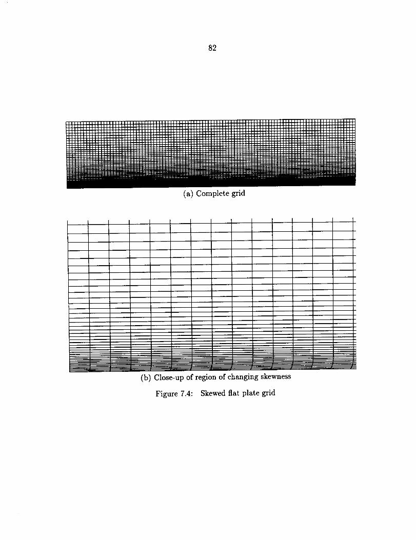
82

(a) Completegrid

J l , ] J

(b) Close-up of region of changing skewness

Figure 7.4: Skewed flat plate grid

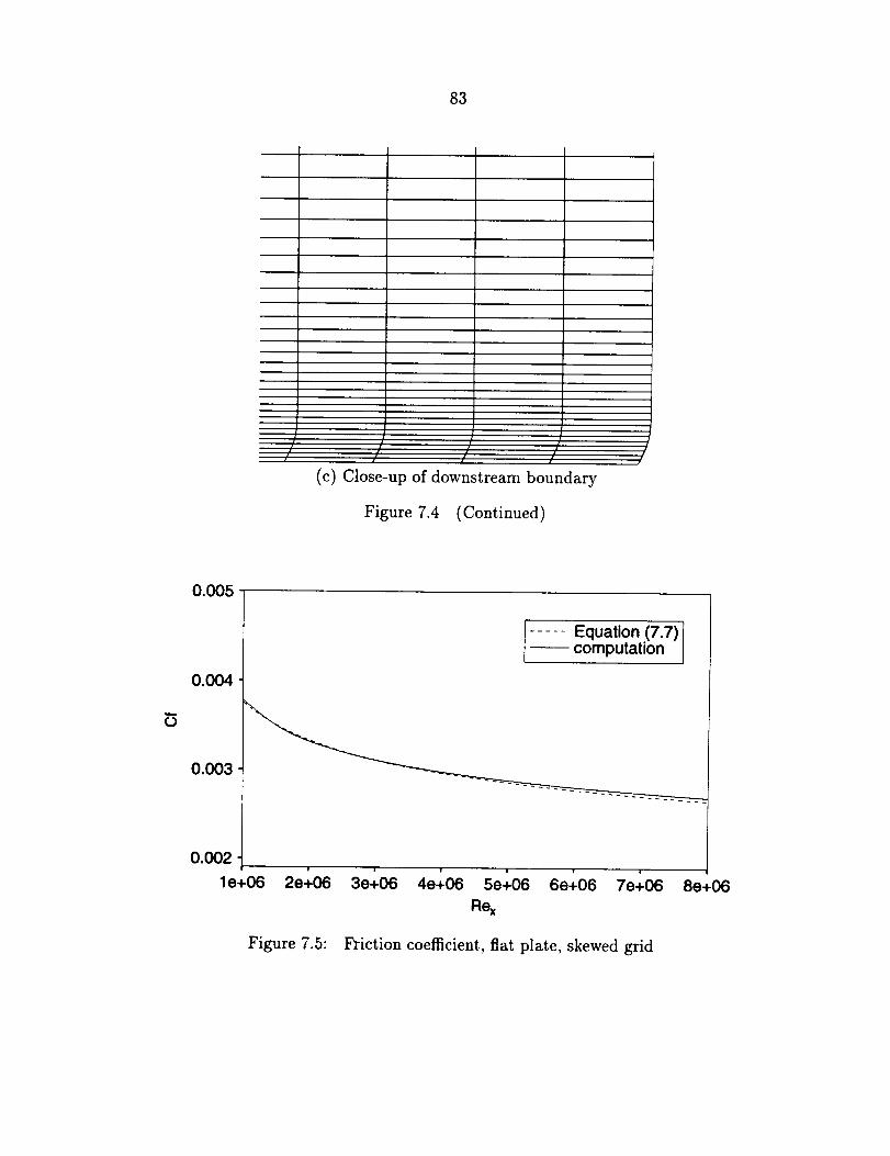
83

J

(c) Close-up of downstream boundary

/

Figure 7.4 (Continued)

0.005

(D

0.004

0.003

0.002w

le+06 2e+06

..... Equation (7.7)

computation

| ! | m

3e+06 4e+06 5e+06 60+06 7e+06

R_

80+06

Figure 7.5: Friction coefficient, flat plate, skewed grid

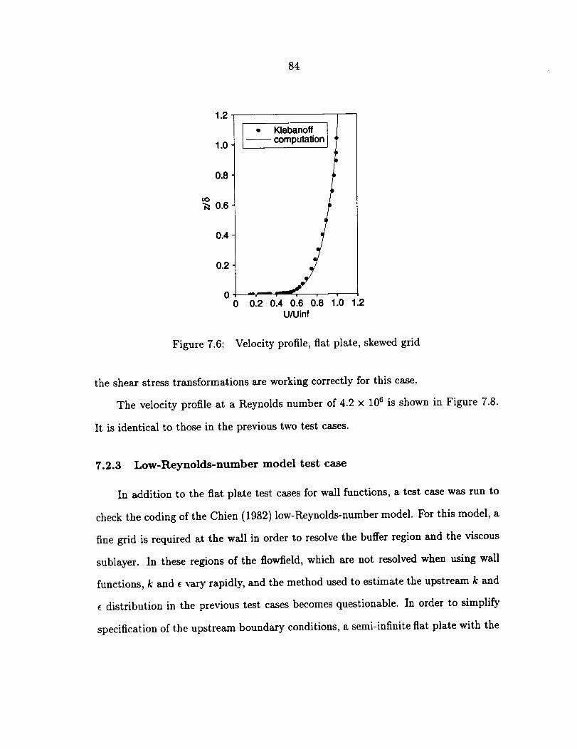
84

1.2

1.0

0.8

_O

"_ 0.6

0.4

0.2

• Klebanoffcomputation

0 1.2

_tlll (

_1 . i i

0.20.40.6 o'.s11oU/Uinf

Figure 7.6: Velocity profile, flat plate, skewed grid

the shear stress transformations are working correctly for this case.

The velocity profile at a Reynolds number of 4.2 x 106 is shown in Figure 7.8.

It is identical to those in the previous two test cases.

7.2.3 Low-Reynolds-number model test case

In addition to the flat plate test cases for wall functions, a test case was run to

check the coding of the Chien (1982) low-Reynolds-number model. For this model, a

fine grid is required at the wall in order to resolve the buffer region and the viscous

sublayer. In these regions of the fiowfield, which are not resolved when using wall

functions, k and e vary rapidly, and the method used to estimate the upstream k and

e distribution in the previous test cases becomes questionable. In order to simplify

specification of the upstream boundary conditions, a semi-infinite flat plate with the

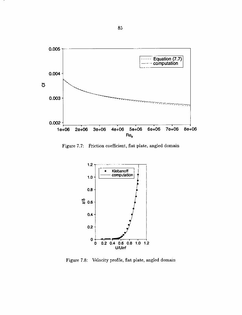
85

0.005

0

0.004

0.003

0.002

..... Equation (7.7)computation

I w w ! , w

le+06 2e+06 3e+06 4e+06 5e+06 6e+06 7e+06 8e+06

Rex

Figure 7.7: Friction coefficient, flat plate, angled domain

1.2

1.0

0.8

oO0.6

0.4

0.2

• Klebanoffcomputation

0 0.2 0.4 0.6 0.8 1.0 1.2UAJinf

Figure 7.8: Velocity profile, flat plate, angled domain

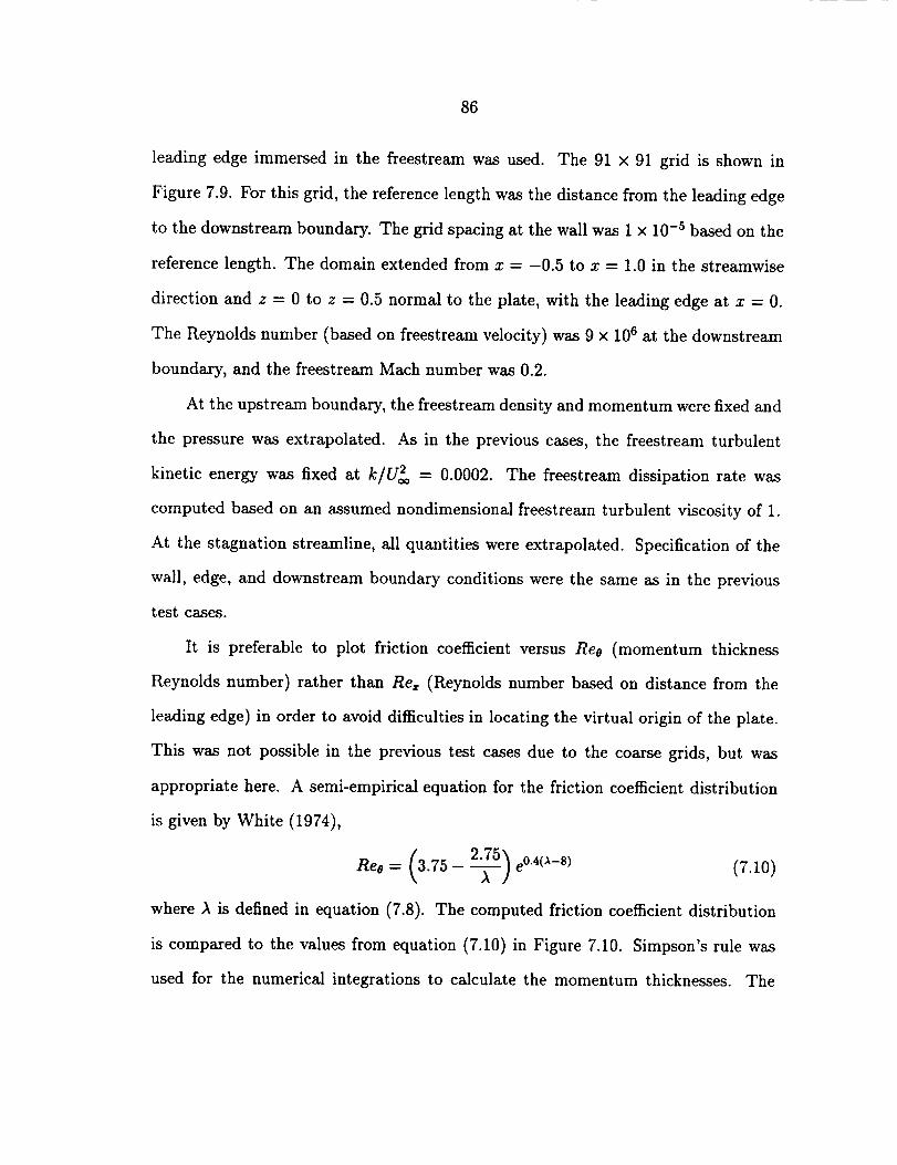
86

leading edge immersed in the freestream was used. The 91 x 91 grid is shown in

Figure 7.9. For this grid, the reference length was the distance from the leading edge

to the downstream boundary. The grid spacing at the wall was 1 x 10 -s based on the

reference length. The domain extended from z = -0.5 to z = 1.0 in the streamwise

direction and z = 0 to z = 0.5 normal to the plate, with the leading edge at x = 0.

The Reynolds number (based on freestrea.m velocity) was 9 x 106 at the downstream

boundary, and the freestream Mach number was 0.2.

At the upstream boundary, the freestream density and momentum were fixed and

the pressure was extrapolated. As in the previous cases, the freestream turbulent

kinetic energy was fixed at k/U 2 = 0.0002. The freestream dissipation rate was

computed based on an assumed nondimensional freestream turbulent viscosity of 1.

At the stagnation streamline, all quantities were extrapolated. Specification of the

wall, edge, and downstream boundary conditions were the same as in the previous

test cases.

It is preferable to plot friction coefficient versus Reo (momentum thickness

Reynolds number) rather than Re,, (Reynolds number based on distance from the

leading edge) in order to avoid difficulties in locating the virtual origin of the plate.

This was not possible in the previous test cases due to the coarse grids, but was

appropriate here. A semi-empirical equation for the friction coefficient distribution

Ree=(3.75 2_5) e°'4(x-s)

is given by White (1974),

(7.10)

where A is defined in equation (7.8). The computed friction coefficient distribution

is compared to the values from equation (7.10) in Figure 7.10. Simpson's rule was

used for the numerical integrations to calculate the momentum thicknesses. The

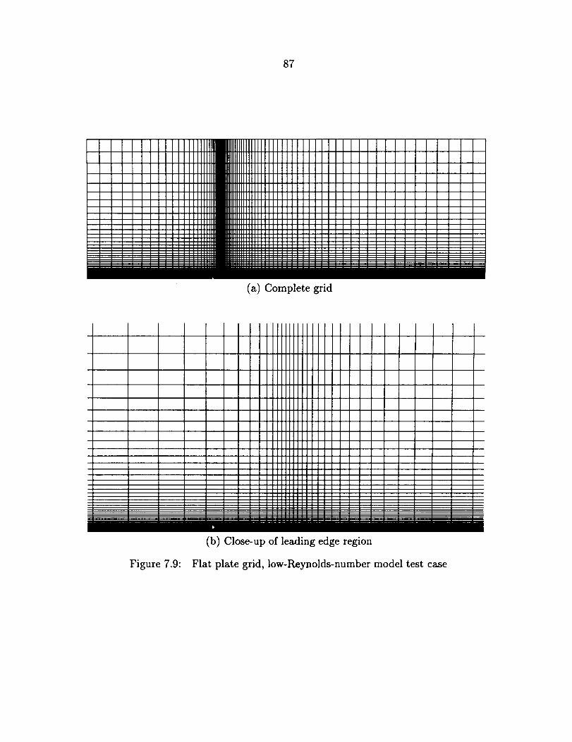
87

(a) Complete grid

i iiiii i ii i i ii

:::::

II:::

:::::

:::::

;::::

:::::

;;;;;:::::

JiJiiI111!!!1!!!!!ii

I

l

ill liD ami/ill Hi i I i Hi(b) Close-up of leading edge region

i

I

, iI

IIIll llil

Figure 7.9: Flat plate grid, low-Reynolds-number model test case

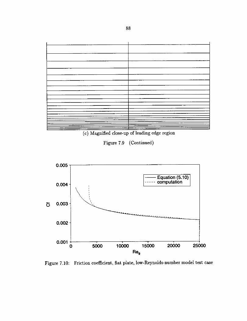
88

(c) Magnified close-upof leadingedgeregion


0.005

0.004

0.003

0.002

0.0010

..... Equation (5.10)computation)

_0 w v 110000 15000 20000 25000

Re e

Figure 7.10: Friction coefficient, flat plate, low-Reynolds-number model test case

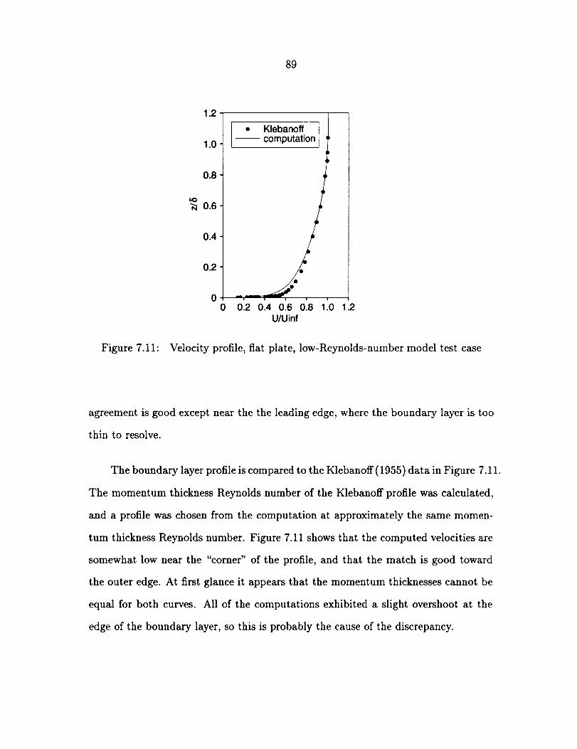
89

1.2

1.0

0.8

_o0.6

0.4

0.2

0

• Klebanoff ]-- computation

I

0 1.0 1.2! t

0.2 0.4 0.6 0.8U/Uinf

Figure 7.11: Velocity profile, fiat plate, low-Reynolds-number model test case

agreement is good except near the the leading edge, where the boundary layer is too

thin to resolve.

The boundary layer profile is compared to the Klebanoff (1955) data in Figure 7.11.

The momentum thickness Reynolds number of the Klebanoff profile was calculated,

and a profile was chosen from the computation at approximately the same momen-

tum thickness Reynolds number. Figure 7.11 shows that the computed velocities are

somewhat low near the "corner" of the profile, and that the match is good toward

the outer edge. At first glance it appears that the momentum thicknesses cannot be

equal for both curves. All of the computations exhibited a slight overshoot at the

edge of the boundary layer, so this is probably the cause of the discrepancy.

9O

7.3 Body of Revolution

7.3.1 Introduction

The next step was to test the wall function formulation on a curved surface. A

well-behaved (i.e., non-separated) fiowfleld was desirable, since the purpose was to

check the stress tensor transformations, and not yet to deal with the issue of the

effectiveness of wall functions (in general terms) for separated flows.

Ramaprian, Patel, and Choi (1978, 1980) measured surface pressures, friction

coefficients, and velocity profiles for incompressible flow over a body of revolution

at zero and ten degrees angle of attack. The body consisted of half of a prolate

spheroid with a hemispherical nose cap. The zero degree angle of attack case was

computed here using the k - e model with the present wall function formulation as

well as the Baldwin-Lomax (1978) algebraic turbulence model and the Chien (1982)

low-Reynolds-number k - e model. Each model was run using three different grids

to demonstrate the advantage of wall functions for this type of flowfield.

The experimental Reynolds number based on freestream velocity was 2 × 108,

and the freestream Mach number was approximately 0.06. The computations were

run at the test Reynolds number, but the freestream Mach number was raised to

0.10 to avoid the incompressible limit of the code while still maintaining essentially

incompressible flow. In the experiment, the boundary layer was tripped near the nose

(x = 0.04), so that the computations were run completely turbulent.

Since the problem was symmetric about the centerline of the body, only half of

the domain was solved. All grids were generated using the hyperbolic scheme of Chan

and Steger (1991). Initially, an elliptic scheme was tried, but it proved impossible to

91

maintain the desiredwall spacing.The hyperbolicschemepermitted excellentcontrol

overwall spacing,ran extremely fast, and waseasyto use.

All distancesin this sectionare normalizedby the length of the body.

7.3.2 Fine grid

For the first grid, a wall spacingwasdesiredthat wouldprovideadequateresolu-

tion for the Baldwin-Lomax and Chienmodelswithout requiring anexcessivenumber

of grid points. A wall spacingof Az + _ 4 was chosen to provide at least one point in

the viscous sublayer, giving a spacing at the wall of 5 x 10 -5 in units of body length.

The grid is stretched geometrically normal to the body using a stretching ratio of

1.11. This relatively conservative value was chosen to minimize numerical errors due

to grid stretching.

Although the location of the outer edge of the domain cannot be precisely speci-

fied when using hyperbolic grid generation, the desired value can be approximated. A

value of twenty body lengths was chosen to minimize boundary proximity effects. A

relationship between wall spacing, domain size, number of grid points, and geometric

stretching ratio is given by Lewis and Pletcher (1986),

Azw = (K- 1)zmo_K "-1- 1 (7.11)

where Az,_ is the wall spacing, Zmaz is the domain size, n is the number of grid points,

and K is the stretching ratio. Solving for n,

log[i + _-(K-Az,__ 1)] (7.12)n = 1 + log(K)

For the present case, this equation yields n = 104. In the streamwise direction,

101 grid points were deemed sufficient for reasonable resolution. The body in the

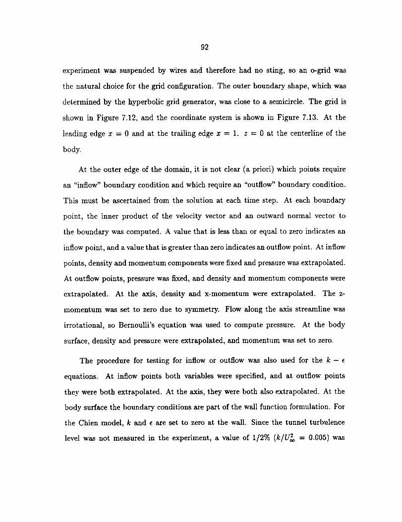
92

experiment was suspendedby wires and therefore had no sting, so an o-grid was

the natural choice for the grid configuration. The outer boundary shape, which was

determined by the hyperbolic grid generator, was close to a semicircle. The grid is

shown in Figure 7.12, and the coordinate system is shown in Figure 7.13. At the

leading edge x = 0 and at the trailing edge x = 1. z = 0 at the centerline of the

body.

At the outer edge of the domain, it is not clear (a priori) which points require

an "inflow" boundary condition and which require an "outflow" boundary condition.

This must be ascertained from the solution at each time step. At each boundary

point, the inner product of the velocity vector and an outward normal vector to

the boundary was computed. A value that is less than or equal to zero indicates an

inflow point, and a value that is greater than zero indicates an outflow point. At inflow

points, density and momentum components were fixed and pressure was extrapolated.

At outflow points, pressure was fixed, and density and momentum components were

extrapolated. At the axis, density and x-momentum were extrapolated. The z-

momentum was set to zero due to symmetry. Flow along the axis streamline was

irrotational, so Bernoulli's equation was used to compute pressure. At the body

surface, density and pressure were extrapolated, and momentum was set to zero.

The procedure for testing for inflow or outflow was also used for the k - e

equations. At inflow points both variables were specified, and at outflow points

they were both extrapolated. At the axis, they were both also extrapolated. At the

body surface the boundary conditions are part of the wall function formulation. For

the Chien model, k and e are set to zero at the wall. Since the tunnel turbulence

level was not measured in the experiment, a value of 1/2% (k/U_ = 0.005) was

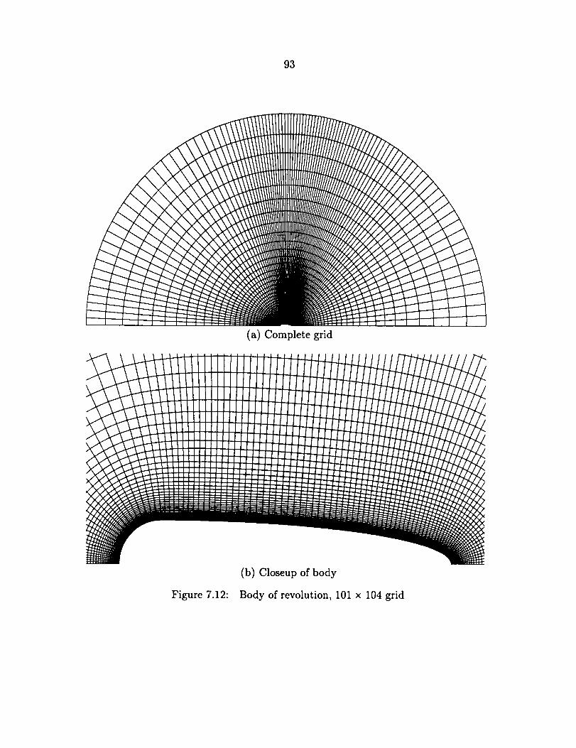
93

(a) Completegrid

(b) Closeupof body

Figure 7.12: Body of revolution, 101 x 104 grid

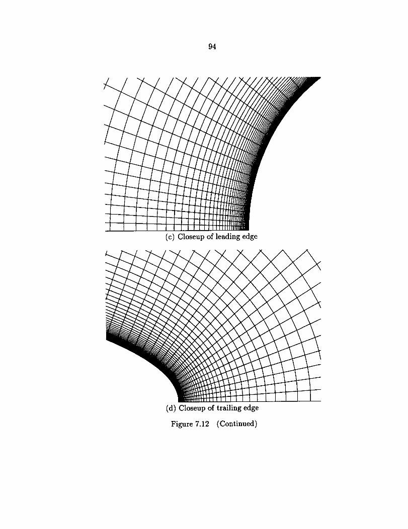
94

(c) Closeupof leading edge

(d) Closeup of trailing edge


95

Z

Figure 7.13:

Dr

X

Body of revolution coordinate system

assumed. A freestream turbulent viscosity of 0.1 (nondimensional) was assumed, and

freestream e was calculated from equation (3.6).

Computed boundary-layer profiles are often affected adversely by even modest

amounts of smoothing (Kaynak and Flores 1987). Since the physical shear stresses

become large near walls, smoothing may be decreased in this region without causing

the computation to become unstable. Various techniques of rolling off smoothing

were tried, but the best solution was to simply turn the smoothing off at the seven

grid points adjacent to the wall.

The computed pressure coefficient distribution is compared with the experimen-

tal data in Figure 7.14. All three turbulence models give good results, with a small

discrepancy near x = 0.1. The discrepancy could be alleviated by increasing the grid

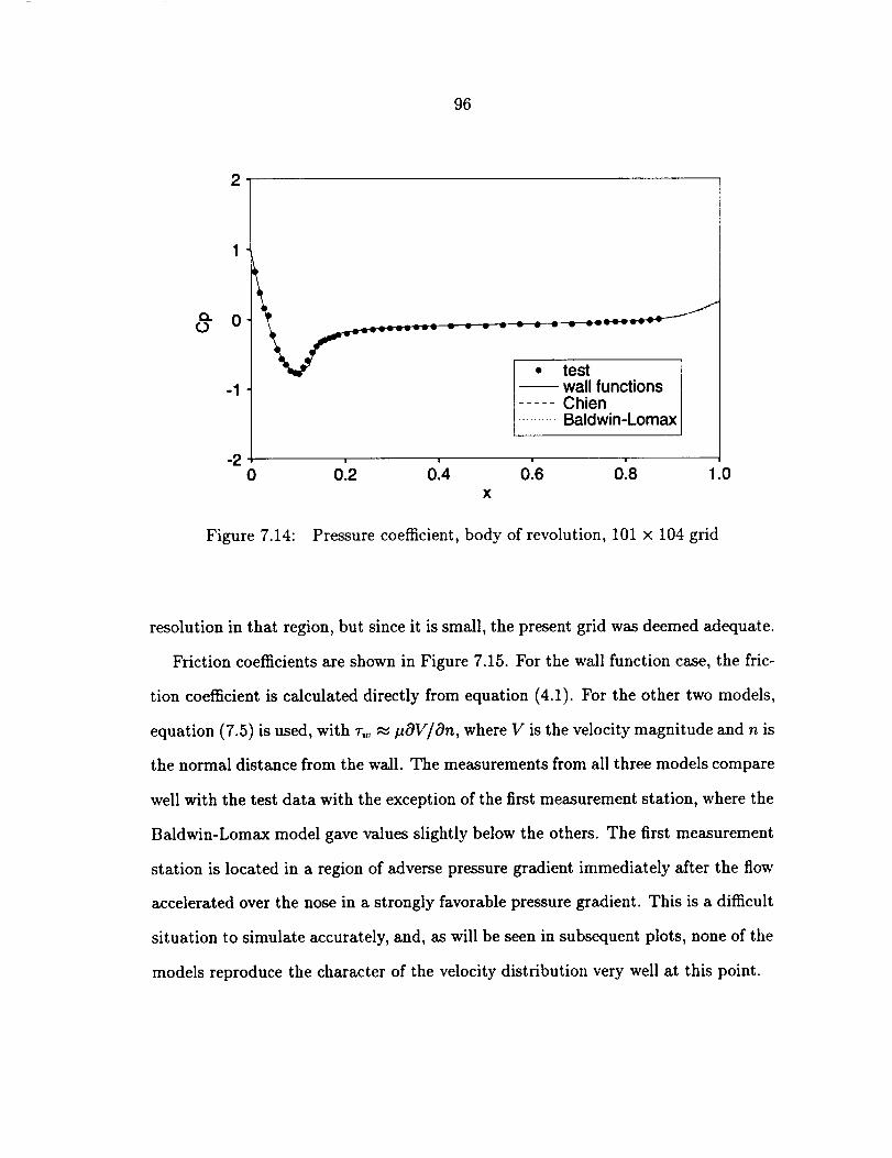
96

2

-1

-2

-- wall functions..... Chien.......... Baldwin-Lomax

i m i |

0 0.2 0.4 0.6 0.8 1.0

Figure 7.14: Pressure coefficient, body of revolution, 101 x 104 grid

resolution in that region, but since it is small, the present grid was deemed adequate.

Priction coefficients are shown in Figure 7.15. For the wall function case, the fric-

tion coefficient is calculated directly from equation (4.1). For the other two models,

equation (7.5) is used, with 7"_o_, pcgV/i)n, where V is the velocity magnitude and n is

the normal distance from the wall. The measurements from all three models compare

well with the test data with the exception of the first measurement station, where the

Baldwin-Lomax model gave values slightly below the others. The first measurement

station is located in a region of adverse pressure gradient immediately after the flow

accelerated over the nose in a strongly favorable pressure gradient. This is a difficult

situation to simulate accurately, and, as will be seen in subsequent plots, none of the

models reproduce the character of the velocity distribution very well at this point.

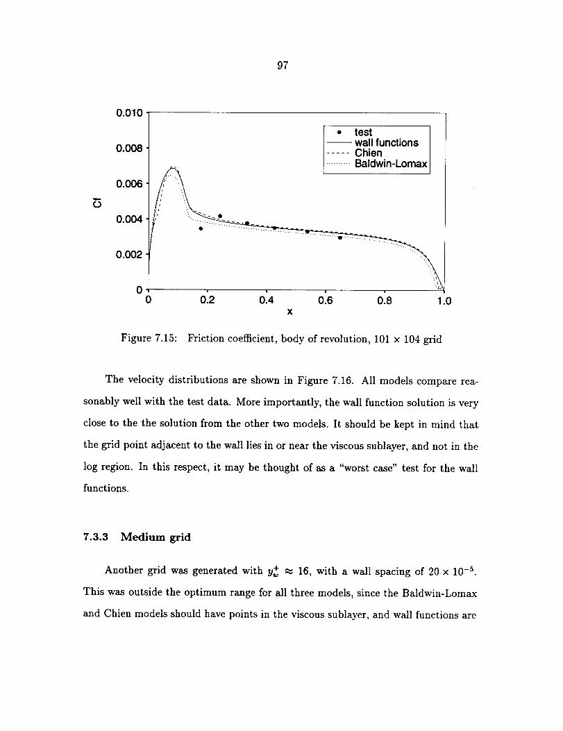
97

¢D

0.010

0.008

0.006

0.004

0.002

00

• test-- wall functions..... Chien.......... Baldwin-Lomax

• .......D "

0.2 0.4 0.6 0.8 1.0X

Figure 7.15: Friction coefficient, body of revolution, 101 x 104 grid

The velocity distributions are shown in Figure 7.16. All models compare rea-

sonably well with the test data. More importantly, the wall function solution is very

close to the the solution from the other two models. It should be kept in mind that

the grid point adjacent to the wall lies in or near the viscous sublayer, and not in the

log region. In this respect, it may be thought of as a "worst case" test for the wall

functions.

7.3.3 Medium grid

Another grid was generated with y+ _, 16, with a wall spacing of 20 x 10 -5.

This was outside the optimum range for all three models, since the Baldwin-Lomax

and Chien models should have points in the viscous sublayer, and wall functions are

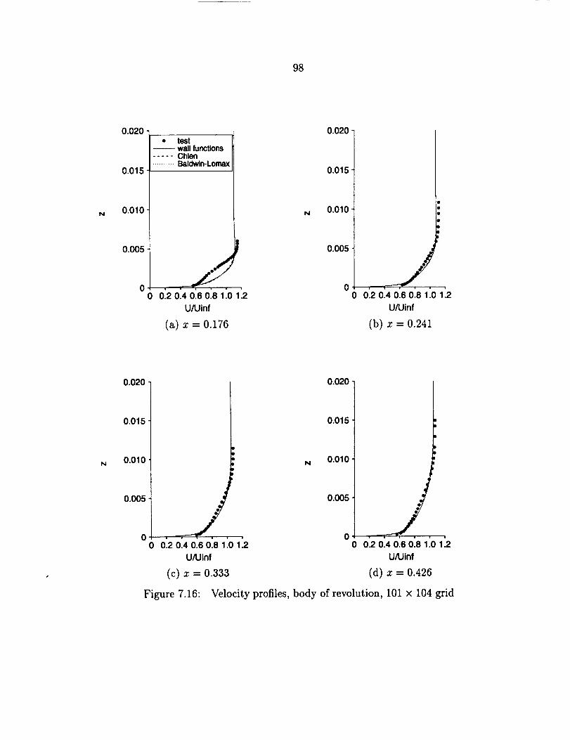
98

N

0.020

0.015

0.010

0.005

00

, test-- wall functions..... Chlen.......... Baldwin-Lomax

f012 014 016 018 110 112

UAJinf

(a) x = 0.176

0.020

0.015

N 0.010

0.005

J0'.2 014 016 018 110 1'.2

UAJinf

(b) x = o.24z

0.020 0.020

N

0.015

0.010

0.005-

I

]o . .---_.E .

0 0.2 0.4 0.6 0.8 1.0 1.2

U/Uinf

(c) x = 0.333

Figure 7.16:

0.015

N 0.010

0.005

q

0 012 0.4 0.6 0.8 1.0 1.2

U/Uinf

(d) x - 0.426

Velocity profiles, body of revolution, 101 × 104 grid

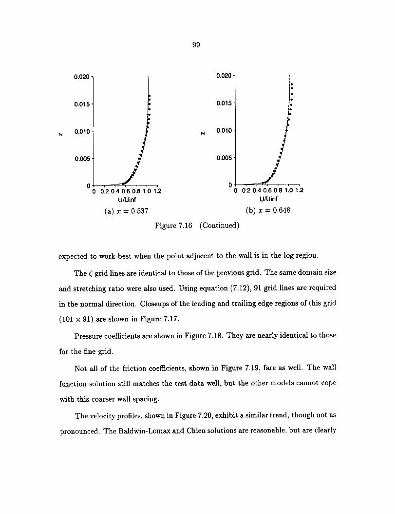
99

N

0.020

0.015

O.OLO

0.005

0.020-

0.015

N 0.010

0.005

0'20'40:6o.e101'.2 00UAJinf

(a) x = 0.537


i , i |

0.2 0.4 0.6 0.8 1.0 112

U/Uinf

(b) x = 0.648

expected to work best when the point adjacent to the wail is in the log region.

The _ grid lines are identical to those of the previous grid. The same domain size

and stretching ratio were also used. Using equation (7.12), 91 grid lines are required

in the normal direction. Closeups of the leading and trailing edge regions of this grid

(101 x 91) are shown in Figure 7.17.

Pressure coefficients are shown in Figure 7.18. They are nearly identical to those

for the fine grid.

Not all of the friction coefficients, shown in Figure 7.19, fare as well. The wail

function solution still matches the test data well, but the other models cannot cope

with this coarser wail spacing.

The velocity profiles, shown in Figure 7.20, exhibit a similar trend, though not as

pronounced. The Baidwin-Lomax and Chien solutions are reasonable, but are clearly

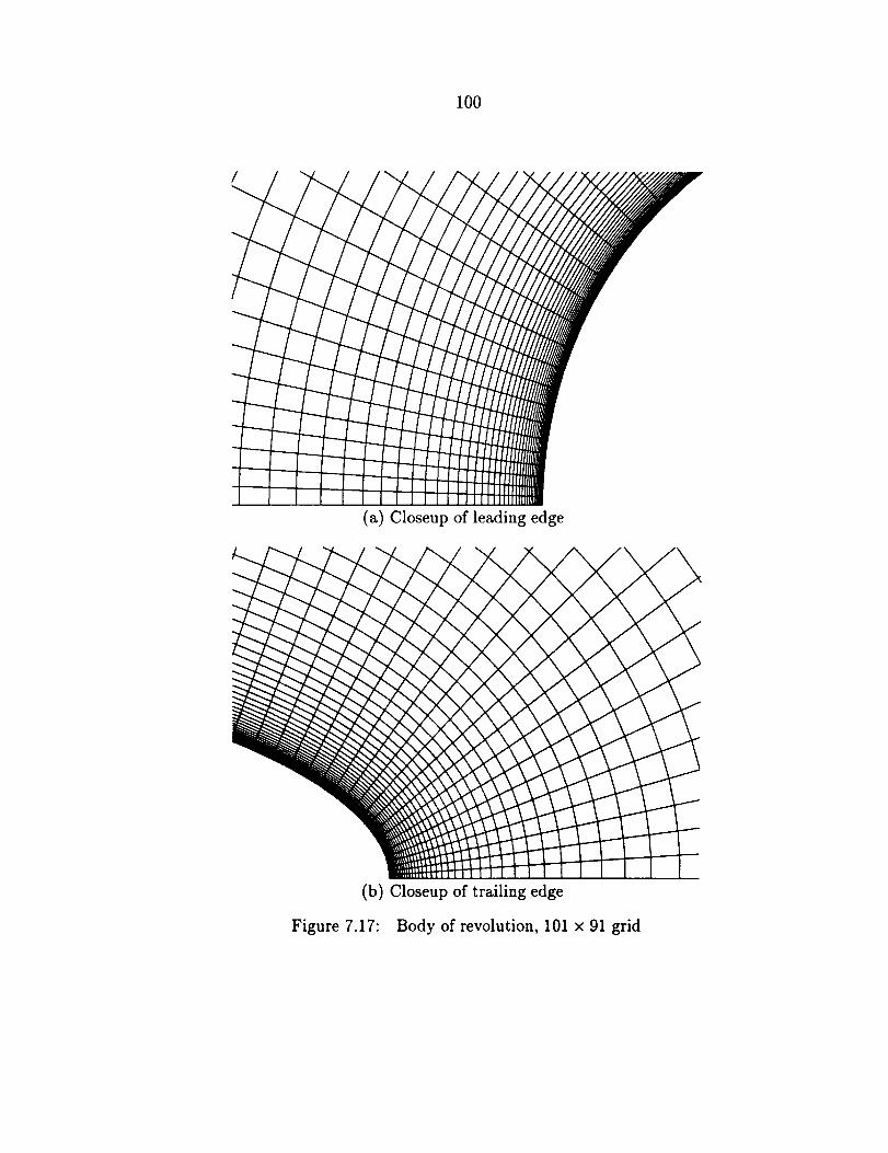
100

(a) Closeupof leadingedge

(b) Closeup of trailing edge


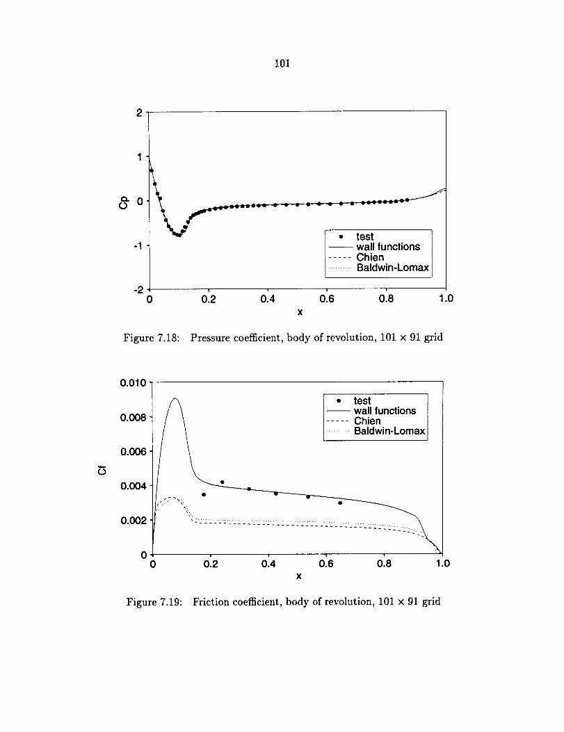
I01

0

-I

-2

• test-- wall functions..... Chien.......... Baldwin-Lomax

! | ! !

0 0.2 0.4 0.6 0.8

X

1.0


0.010

0.008

0.006

0.004

0.002

0

_= teaSl_function s

..... Chien

_Baldwi__ _ n-Lomax

' ' ' 0"8.0 0.2 0.4 0.6 .0

Figure 7.19: Friction coefficient, body of revolution, 101 × 91 grid

102

deficient as comparedto the previoussolution, while the wall function solution still

looks good.

7.3.4 Coarse grid

A final grid wasgeneratedwith Az + _ 48, or 60 × 10 -5 in physical coordinates.

Closeups of the leading and trailing edge regions of this grid (101 x 80) are shown in

Figure 7.21. The results for this grid are shown in Figures 7.22, 7.23, and 7.24.

The 101 x 80 grid is clearly too coarse for the Chien and Baldwin-Lomax models,

while the wall function solution still looks good. It should be noted that the wall

function solutions for the different grids show some small differences. In the 101 × 80

grid, the point adjacent to the wall is in the log region, while this is not true for

the other two finer grids. The boundary conditions for k and e are more rigorous

for points in the log region, as was discussed in the "Wall Functions" chapter. The

different approaches are therefore expected to affect the results.

7.4 Prolate Spheroid

7.4.1 Introduction

Computation of the flow over a prolate spheroid at angle of attack is a partic-

ularly challenging problem for CFD. There exist regions of favorable and adverse

pressure gradients, the flow on the leeward side may be massively separated, and

laminar, transition, and turbulent regimes are frequently encountered.

In the late 1970's and early 1980's, a series of experiments was carried out at

DFVLR (Deutsche Forschungs- und Versuchsanstalt fiir Luft- und Raumfahrt) to

obtain detailed measurements of the surface flow on a prolate spheroid at angle of

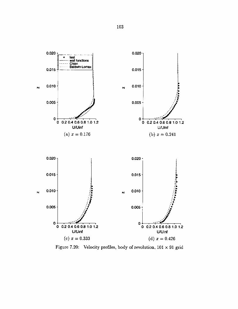
103

N

0.020 -

0.015 -

0.010 -

0.005 -

• test-- wall functions

..... Chlen

.......... Baldwin-Lomax

/°0 012040608101'.2

U/Uinf

(a_ x = 0.176

0.020

N

0.015

0.010

0.005 j

00 0120.4080.810,12U/Uinf

(b) x = 0.241

0.020 0.020

N

0.015

0.010

0.005

Figure 7.20:

0.015

J

, N 0.010 ,'ii,

f i,

,/ 0.005 ,i /

0 0.2 0.4 0.6 0.8 1.0 112 0 .......0 0:2040.60.81.01:2U/Uinf U/Uinf

(c) x = 0.333 (d) x = 0.426

Velocity profiles, body of revolution, 101 x 91 grid

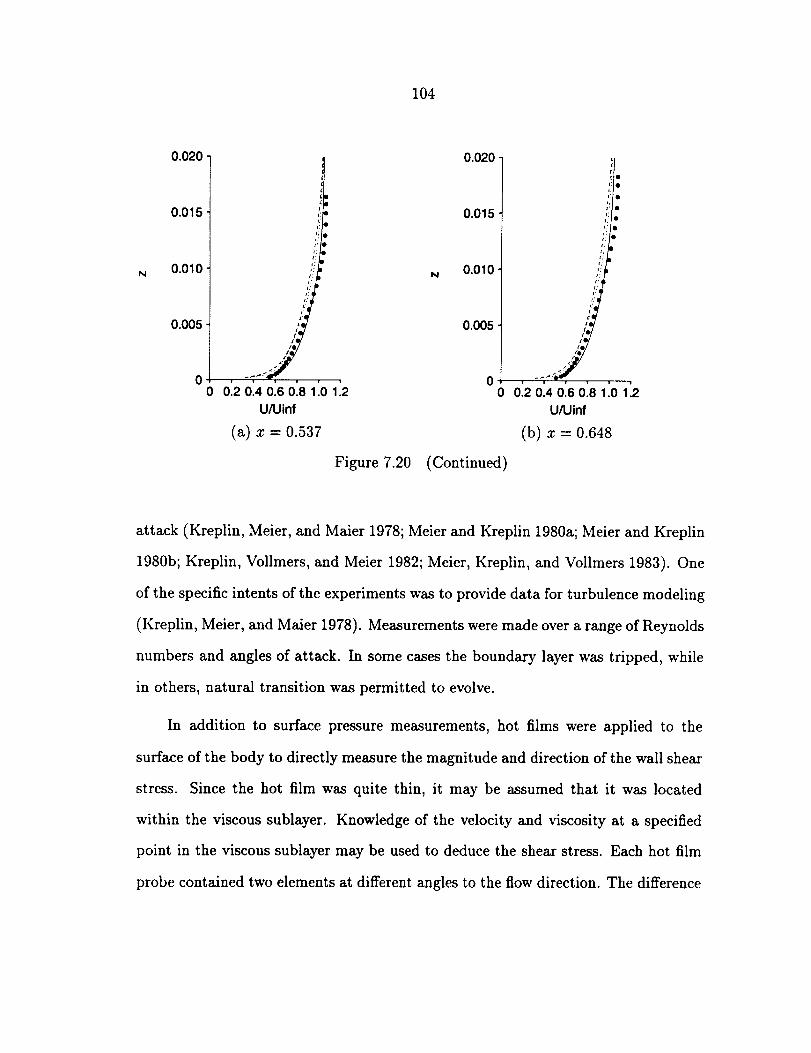
104

N

0.020

0.015

0.010

0.005

S

(

/,

__

0 0:2 0.4 0.6 0.8 1.0 1:2

U/Uinf

(a) x = 0.537\ /

Figure 7.20

0.020

0.015

0.010

0.005

o

J:ql

I:I:

L;I[

I.'I:

L"

I!;'

'2'te

, i i

0 0120.40.80.81101'.2U/Uinf

(b) x = 0.648

(Continued)

attack (Kreplin, Meier, and Maier 1978; Meier and Kreplin 1980a; Meier and Kreplin

1980b; Kreplin, Vollmers, and Meier 1982; Meier, Kreplin, and Vollmers 1983). One

of the specific intents of the experiments was to provide data for turbulence modeling

(Kreplin, Meier, and Maier 1978). Measurements were made over a range of Reynolds

numbers and angles of attack. In some cases the boundary layer was tripped, while

in others, natural transition was permitted to evolve.

In addition to surface pressure measurements, hot films were applied to the

surface of the body to directly measure the magnitude and direction of the wall shear

stress. Since the hot film was quite thin, it may be assumed that it was located

within the viscous sublayer. Knowledge of the velocity and viscosity at a specified

point in the viscous sublayer may be used to deduce the shear stress. Each hot film

probe contained two elements at different angles to the flow direction. The difference

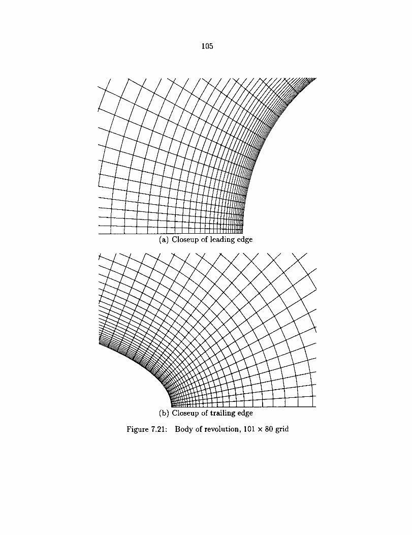
105

(a) Closeupof leadingedge

(b) Closeupof trailing edge


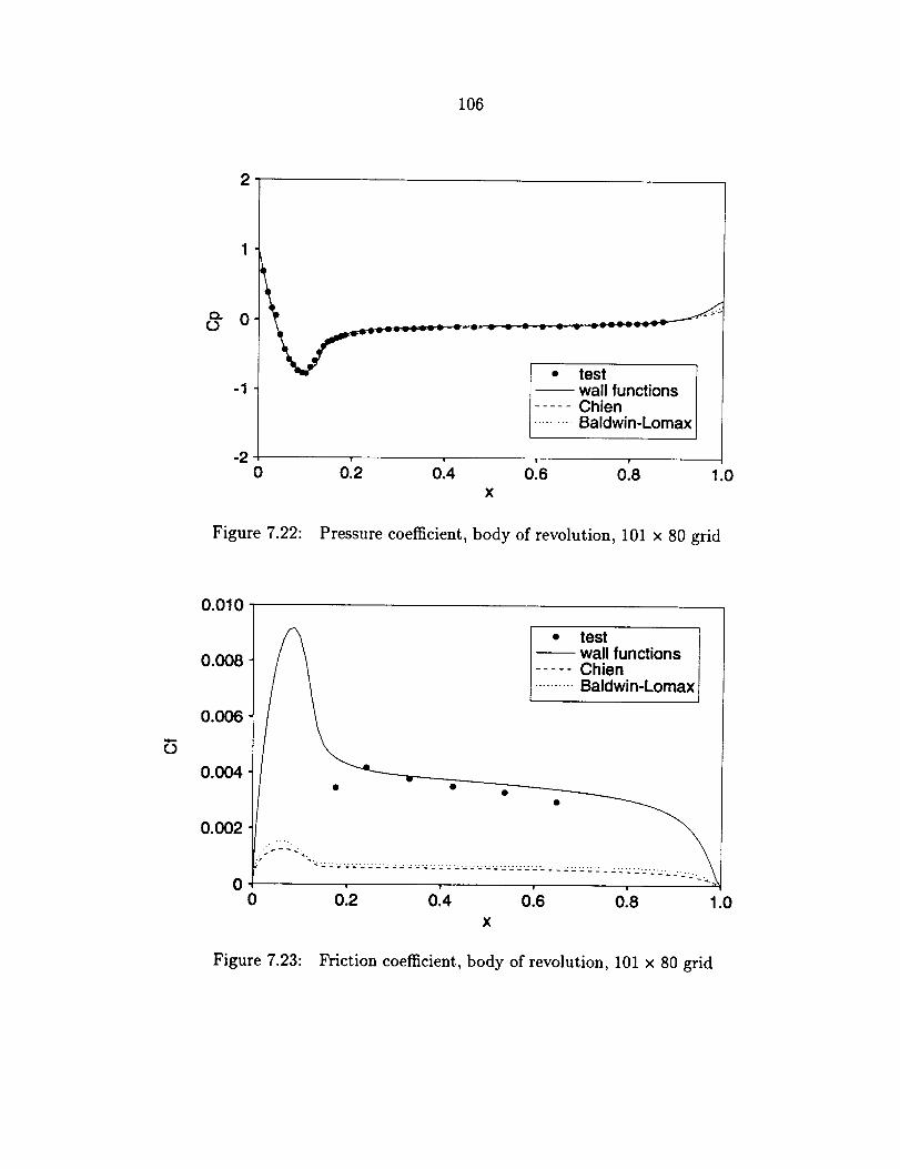
106

2

-1

-2

J test 1wall functions I

- Chien r_ galdwin.Lomaxl

' i ' '0 0.2 04 0.6 0.8 1.0X


o.olo1 /_• test j

J / \ - wall functions J0.008 | / / ..... Chien. I

.......... o

0.006

0.004

0.002

00 0.2 0.4 0.6 0.8

X

1.0

Figure 7.23: Friction coefficient, body of revolution, 101 x 80 grid

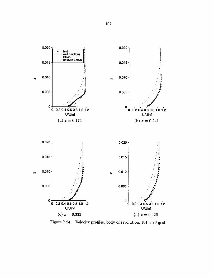
107

N

0.020

0.015

0.010

0.005

• test-- wall functions..... Chlen.......... Baldwtn-Lomax

i .i .'

/s ..

0.2 0.4 0.6 0.8 1.0 112

U/Uinf

(a) x = 0.176

0.020

0.015

N 0.010

0.005

i

0 0120.40.60.81.01:2U/Uinf

(b) x = 0.241

0.020 0.020

N

0.015

0.010

0.005

0

=1

ji

iIJ

/J

i :

.," :'. _.__' ''::'

0 012 0.4 0.6 0.8 1.0 112

U/Uinf

(c) x = 0.333

Figure 7.24:

0.015

N 0.010

0.005

l

/ :

i /

i. •

o o'.20.40.60.81.o112U/Uinf

(d) x = 0.426

Velocity profiles, body of revolution, 101 x 80 grid

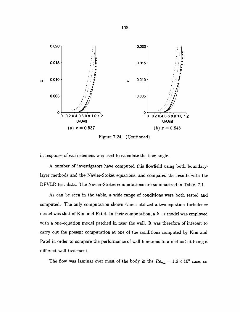
108

N

0.020

0.015

0.010

0.005

00

i

f

;it :i ,f ,: qi :j.,

r ."

j/ o

,

0120.4 0.6 0.8 1.0 1;2

U/Uinf

(a) x = 0.537

Figure 7.24

0.020 -

0.015 -

N 0.010

0.005

/ •i

/S :

[

r

i 1

p .

J ..: ° °

(Continued)

00 0:2 0.4 0.6 0.8 1:0 1:2

U/Uinf

(b) x = 0.648

in response of each element was used to calculate the flow angle.

A number of investigators have computed this flowfield using both boundary-

layer methods and the Navier-Stokes equations, and compared the results with the

DFVLR test data. The Navier-Stokes computations are summarized in Table 7.1.

As can be seen in the table, a wide range of conditions were both tested and

computed. The only computation shown which utilized a two-equation turbulence

model was that of Kim and Patel. In their computation, a k - e model was employed

with a one-equation model patched in near the wall. It was therefore of interest to

carry out the present computation at one of the conditions computed by Kim and

Patel in order to compare the performance of wall functions to a method utilizing a

different wall treatment.

The flow was laminar over most of the body in the Reuo= = 1.6 x 106 case, so

109

the case at a = 10 ° and Re,,_ = 7.2 x 106 was chosen for the present study. Another

advantage of this case was that rather than tripping the boundary layer, it was

permitted to go through natural transition to turbulence. This permitted trying a

different method of forcing the transition point in the k - e model (as compared

to Kim and Patel). A freestream Mach number of 0.20 was chosen to minimize

compressibility effects without excessively hindering convergence.

The use of wall functions is challenging for such a flow, due to the three-

dimensionality of the boundary layer. In discussing their approach to solving this

flowfield, Deng, Piquet, and Queutey (1990) stated that

The wall function approach is avoided in this work so that the equations

... are solved to the wall. For a significant increase in numerical troubles

and of computing time (because the integration is carried out to y+ =

.1 - .3), the delicate problem of the threedimensional [sic] specification of

the log-law is avoided.

7.4.2 Grid

It is desirable to have the grid point adjacent to the wall fall near the bottom

of the log region. Since the values of Ay+ are not known a priori, the following

method was used for an estimate. The definitions of y+ and C I (equations (4.3)

and (7.5)) show that y+ oc _ for a given freestream velocity and viscosity. Using

the flat plate equation (7.4) for a rough estimate of friction coefficient, it may be

shown that y+ cx ln(Re). In the coarse grid test case for the body of revolution,

Re,,® = 7.2 x 106 , the wall spacing was 60 x 10 -5 , and Ay+ _ 48. Using the

above estimate of the variation of y+ with Re,,®, wall spacing of 60 x 10 -5 results

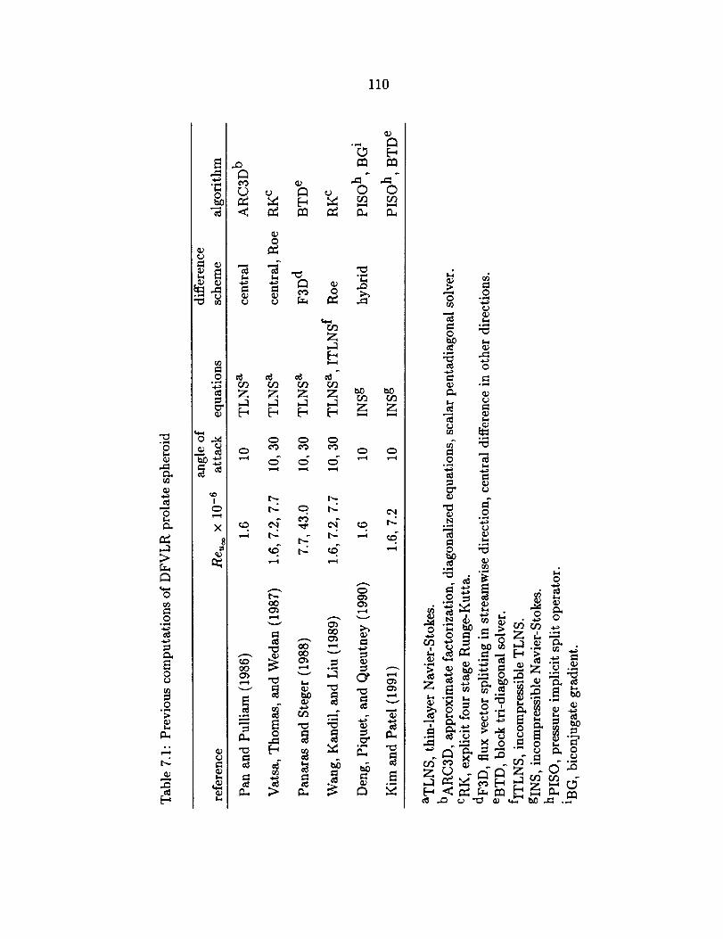
110

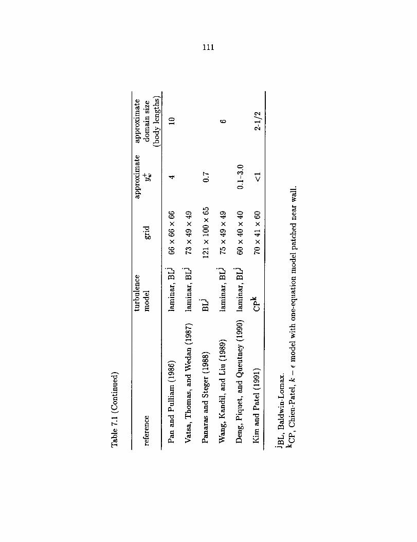
111

°l,--q

0

" r_ t_O

"0

_0

&

c5

u')

XX X

X X ×

X X X

_'_ _ ,_

X X X

._. ._ ._ .=.

co

0

0

.m

"00

I

°_,_

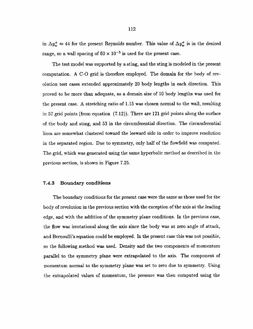
112

in Ay+ _ 44 for the present Reynolds number. This value of Ay+ is in the desired

range, so a wall spacing of 60 x 10 -5 is used for the present case.

The test model was supported by a sting, and the sting is modeled in the present

computation. A C-O grid is therefore employed. The domain for the body of rev-

olution test cases extended approximately 20 body lengths in each direction. This

proved to be more than adequate, so a domain size of 10 body lengths was used for

the present case. A stretching ratio of 1.15 was chosen normal to the wall, resulting

in 57 grid points (from equation (7.12)). There are 121 grid points along the surface

of the body and sting, and 53 in the circumferential direction. The circumferential

lines are somewhat clustered toward the leeward side in order to improve resolution

in the separated region. Due to symmetry, only half of the flowfield was computed.

The grid, which was generated using the same hyperbolic method as described in the

previous section, is shown in Figure 7.25.

7.4.3 Boundary conditions

The boundary conditions for the present case were the same as those used for the

body of revolution in the previous section with the exception of the axis at the leading

edge, and with the addition of the symmetry plane conditions. In the previous case,

the flow was irrotational along the axis since the body was at zero angle of attack,

and Bernoulli's equation could be employed. In the present case this was not possible,

so the following method was used. Density and the two components of momentum

parallel to the symmetry plane were extrapolated to the axis. The component of

momentum normal to the symmetry plane was set to zero due to symmetry. Using

the extrapolated values of momentum, the pressure was then computed using the

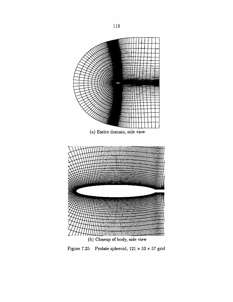
113

(a) Entire domain, sideview

(b) Closeupof body, side view

Figure 7.25: Prolate spheroid, 121 x 53 x 57 grid

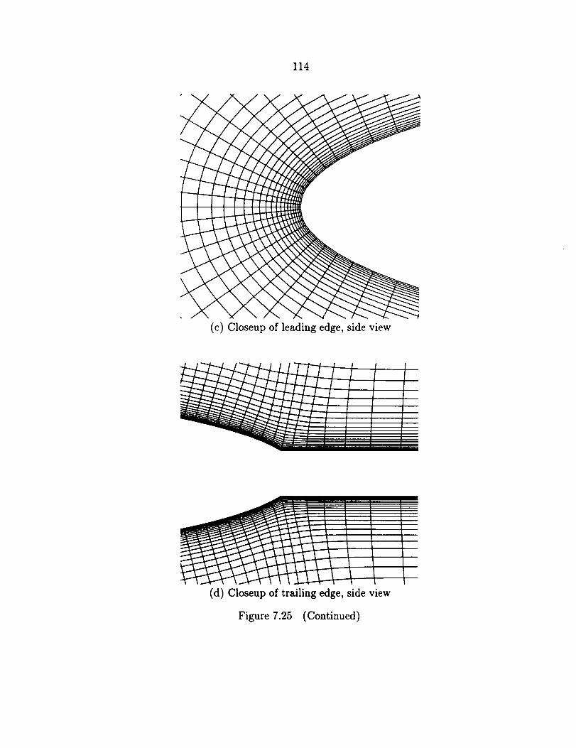
114

(c) Closeupof leadingedge,sideview

(d) Closeupof trailing edge,side view


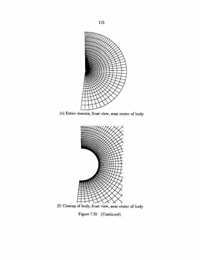
115

(e) Entire domain, front view, near centerof body

(f) Closeupof body, front view, near center of body


116

x-momentum equation. At the symmetry planes,valuesof all dependentvariables

are reflected,e.g. pk=l = Pk=3.

It was found in previous runs that, below a certain level, the freestream turbulent

kinetic energy had little effect on the results. Larger values, however, had a marked

effect. For the small values, any diffusion of turbulent kinetic energy in to the bound-

ary is apparently overwhelmed by the production rate in the boundary layer. Since

the "small" values gave the best agreement with the test data, k/(uoo) 2 = 1 × 10 -8

is used here. A small value is employed, rather than zero, because the source terms

in the pe transport equation contain k in several denominators. A nondimensional

freestream turbulent viscosity of 0.01 was assumed, and the freestream e was calcu-

lated from equation (3.6). The small value of #t was chosen so as not to affect the

laminar flow significantly, as will be clarified below. As in the previous test cases,

lower limiters on both k and e are set to freestream values.

When using algebraic turbulence models, tripping a laminar boundary may be

effected simply by turning the model on at a specified location in the flowfield. This

is possible because the turbulent viscosity is a function of the local flowfield, and his-

tory effects are not considered. With two-equation models, the turbulence quantities

are transported throughout the domain. Kim and Patel (1991) solved the turbu-

lence transport equations over the entire domain, and then, at the end of each step,

overwrote the computed turbulent viscosities with zeros at those points designated

as being laminar. A problem with this approach is that k and e are increasing in

the boundary layer, mostly due to the production terms, in the region of laminar

flow. Their profiles are quite developed by the time the points of forced transition

are reached. In the present study, the time step was set to zero at all laminar grid

117

points. The freestreamvaluesof k and e were therefore maintained at these points,

and the turbulence was permitted to evolve downstream of the trip line. Since a

small freestream value of #t is used, the laminar flow was not significantly affected.

The friction coefficient map taken from Kreplin, Vollmers, and Meier (1982) is

shown in Figure 7.26. The vector lengths are proportional to the measured wall

shear stresses, and they are oriented at the circumferential angles at which the shear

stresses act. It is not possible to deduce a precise transition line from this map, but

an approximate line may be determined from the regions where the friction coefficient

rapidly increases. Figure 7.27 shows an unwrapped surface grid with points marked

at the computational trip line.

7.4.4 Additional considerations

Smoothing coefficients of e4 = 0.10 and e_ = 0.028 were used (see equations (6.79)

and (6.80)), based on several test runs to see how low they could be pushed without

compromising stability.

Friction coefficient angle data were measured in the experiment, based on the

difference in the response of the two elements of the hot-film probes. The friction

coefficient angle, which is assumed to be identical to the flow angle in the compu-

tation, is changing as the wall is approached. The wall spacing is fairly large since

wall functions are being used, and it is therefore difficult to deduce the limit of the

angle at the wall. The flow angle was computed at the grid points near the wall, and

second order Lagrangian extrapolation was used estimate the angle at the wall.

A similar difficulty was encountered in computing the friction coefficient in the

laminar region of the flowfield. Third order Lagrangian interpolation was used to

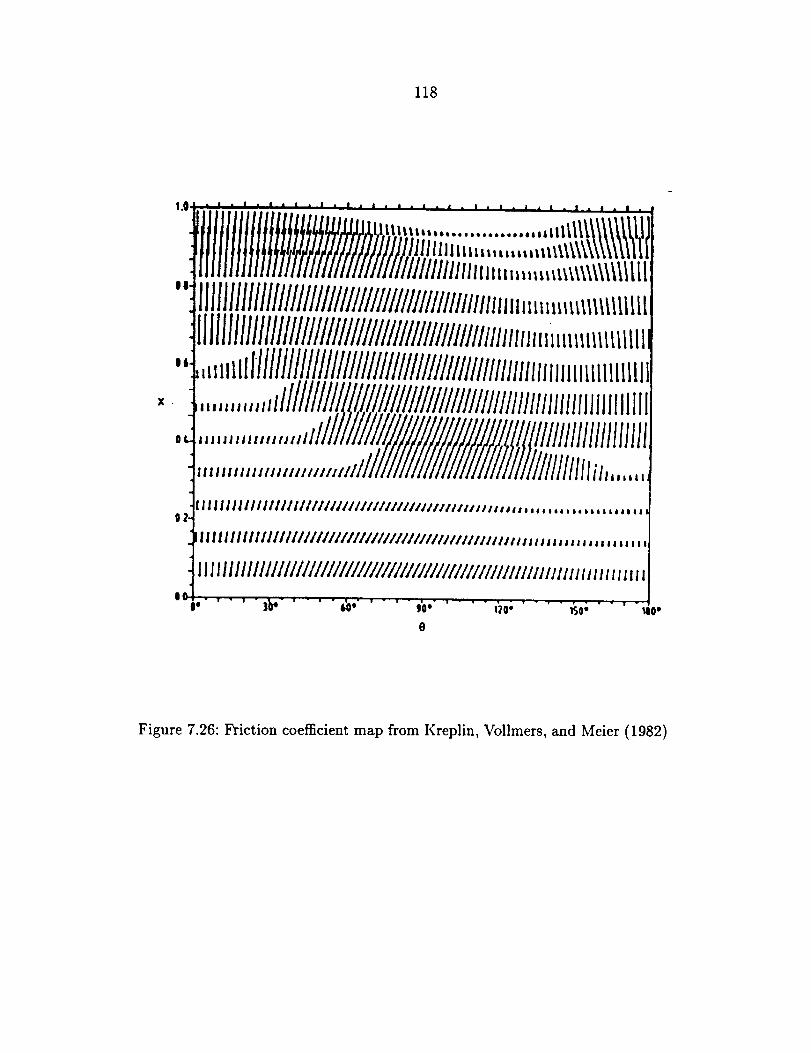
118

1.o • i • i • I • i • I • I • i • ¢ • J • • . I i ! " i i | i I • i • I . !

lllll]llllllllllllllllllllllllllllliii-lilllnnz_tt,,,,,,,,,_\\\\\_lllll

":lilHlllillllllllllllllllllllllllllllll////mm_,_,,,,.,,,_l_lilltllllIllllllllllilllllllllllllil/ll/l/ll//////HlllHn.,,,,,,, lll

" ,,, t lllllill//llllllllllllllllllllllllllilil//Hllnll lj ,t tlllillllx. ,,,,,,,,,,,,flll/I///////_//////illllllllllillllll/lllHllllllliltl

, ,,,,,,,,,,,,,,,,,,1_///////1//1111111111II111t11II111

IlllIIlliillilllllllllllllllllllllllllllllllltttttsa_a,,,,,,,,,,_,,,,,i,t0

Iilllliilllllllllllill/lllllll/lll/llll/lllllllllilllttat_aa_ll,_,,,,,

llllllllllIWll////////////////////////////////WWll/IHlttmttt_tli

o '"i_' io I_0" 150"

Figure 7.26: Friction coefficient map from Kreplin, Vollmers, and Meier (1982)

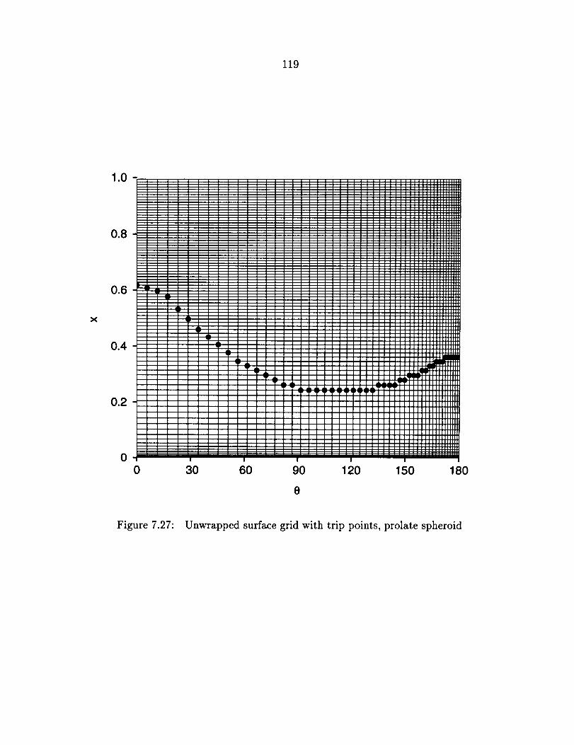
119

X

1o0 -

0.8

0.6

0.4

0.2

0

..2'

i

: i: i

1 !

i •

• dL1,

!

600 30 90 120 150 180

e

Figure 7.27: Unwrapped surface grid with trip points, prolate spheroid

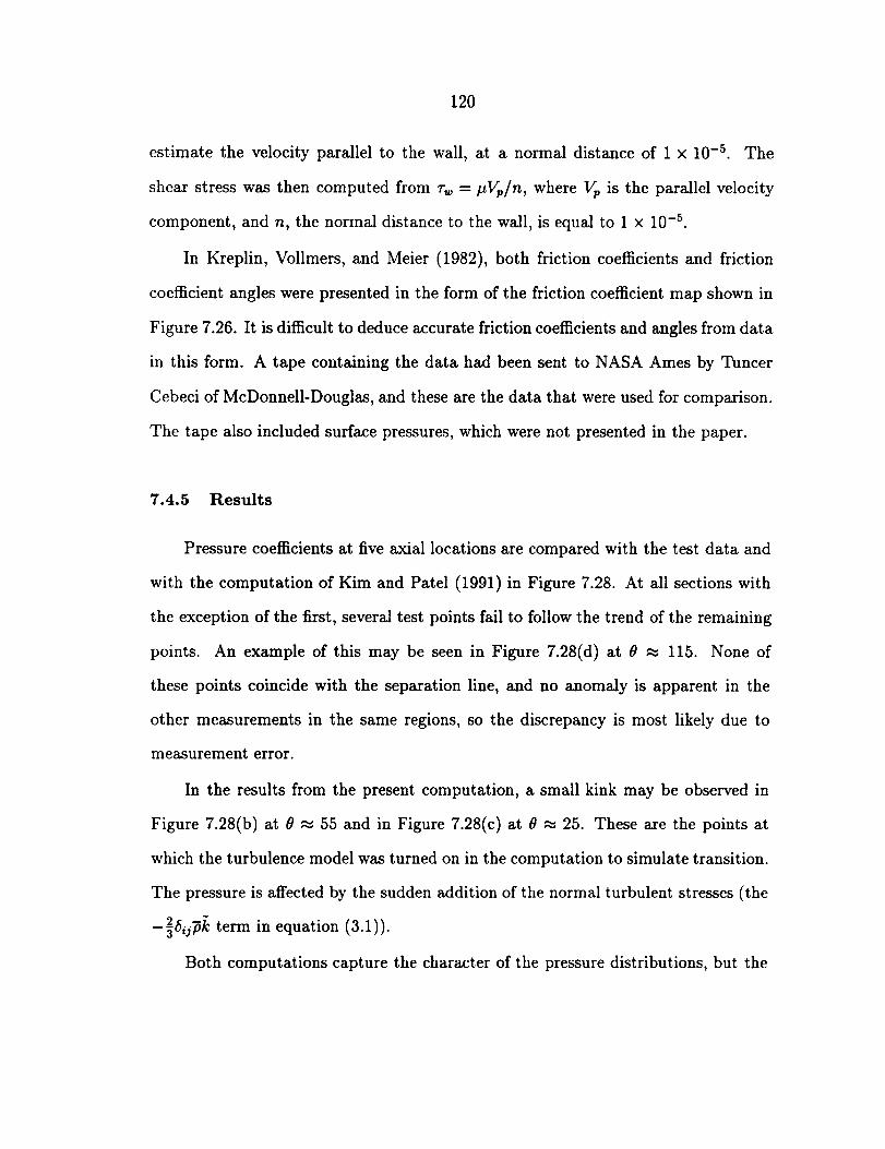
120

estimate the velocity parallel to the wall, at a normal distance of 1 x 10-5. The

shearstresswas then computed from T,,, = pVp/n, where Vp is the parallel velocity

component, and n, the normal distance to the wall, is equal to 1 x 10 -_.

In Kreplin, Vollmers, and Meier (1982), both friction coefficients and friction

coefficient angles were presented in the form of the friction coefficient map shown in

Figure 7.26. It is difficult to deduce accurate friction coefficients and angles from data

in this form. A tape containing the data had been sent to NASA Ames by Tuncer

Cebeci of McDonnell-Douglas, and these are the data that were used for comparison.

The tape also included surface pressures, which were not presented in the paper.

7.4.5 Results

Pressure coefficients at five axial locations are compared with the test data and

with the computation of Kim and Patel (1991) in Figure 7.28. At all sections with

the exception of the first, several test points fall to follow the trend of the remaining

points. An example of this may be seen in Figure 7.28(d) at 0 _ 115. None of

these points coincide with the separation line, and no anomaly is apparent in the

other measurements in the same regions, so the discrepancy is most likely due to

measurement error.

In the results from the present computation, a small kink may be observed in

Figure 7.28(b) at 8 _ 55 and in Figure 7.28(c) at 6 _ 25. These are the points at

which the turbulence model was turned on in the computation to simulate transition.

The pressure is affected by the sudden addition of the normal turbulent stresses (the

-_tSij-fil¢ term in equation (3.1)).

Both computations capture the character of the pressure distributions, but the

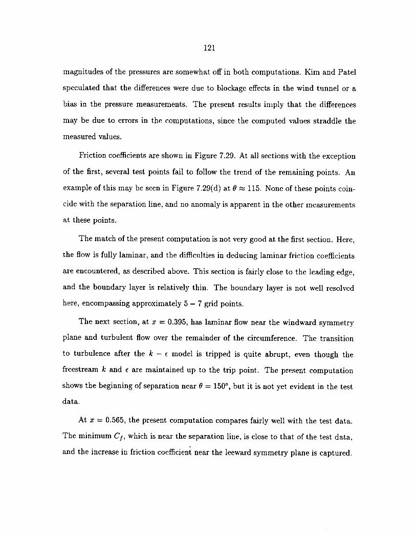
121

magnitudesof the pressuresaresomewhatoff in both computations. Kim and Patel

speculatedthat the differenceswere due to blockageeffectsin the wind tunnel or a

bias in the pressuremeasurements.The present results imply that the differences

may be due to errors in the computations, sincethe computed valuesstraddle the

measuredvalues.

Friction coefficientsareshownin Figure 7.29. At all sectionswith the exception

of the first, several test points fail to follow the trend of the remaining points. An

exampleof this may beseenin Figure 7.29(d) at _ _ 115. None of these points coin-

cide with the separation line, and no anomaly is apparent in the other measurements

at these points.

The match of the present computation is not very good at the first section. Here,

the flow is fully laminar, and the difficulties in deducing laminar friction coefficients

are encountered, as described above. This section is fairly close to the leading edge,

and the boundary layer is relatively thin. The boundary layer is not well resolved

here, encompassing approximately 5 - 7 grid points.

The next section, at x - 0.395, has laminar flow near the windward symmetry

plane and turbulent flow over the remainder of the circumference. The transition

to turbulence after the k - e model is tripped is quite abrupt, even though the

freestream k and e are maintained up to the trip point. The present computation

shows the beginning of separation near/_ -- 150 °, but it is not yet evident in the test

data.

At x - 0.565, the present computation compares fairly well with the test data.

The minimum Cf, which is near the separation line, is close to that of the test data,

and the increase in friction coefficient near the leeward symmetry plane is captured.

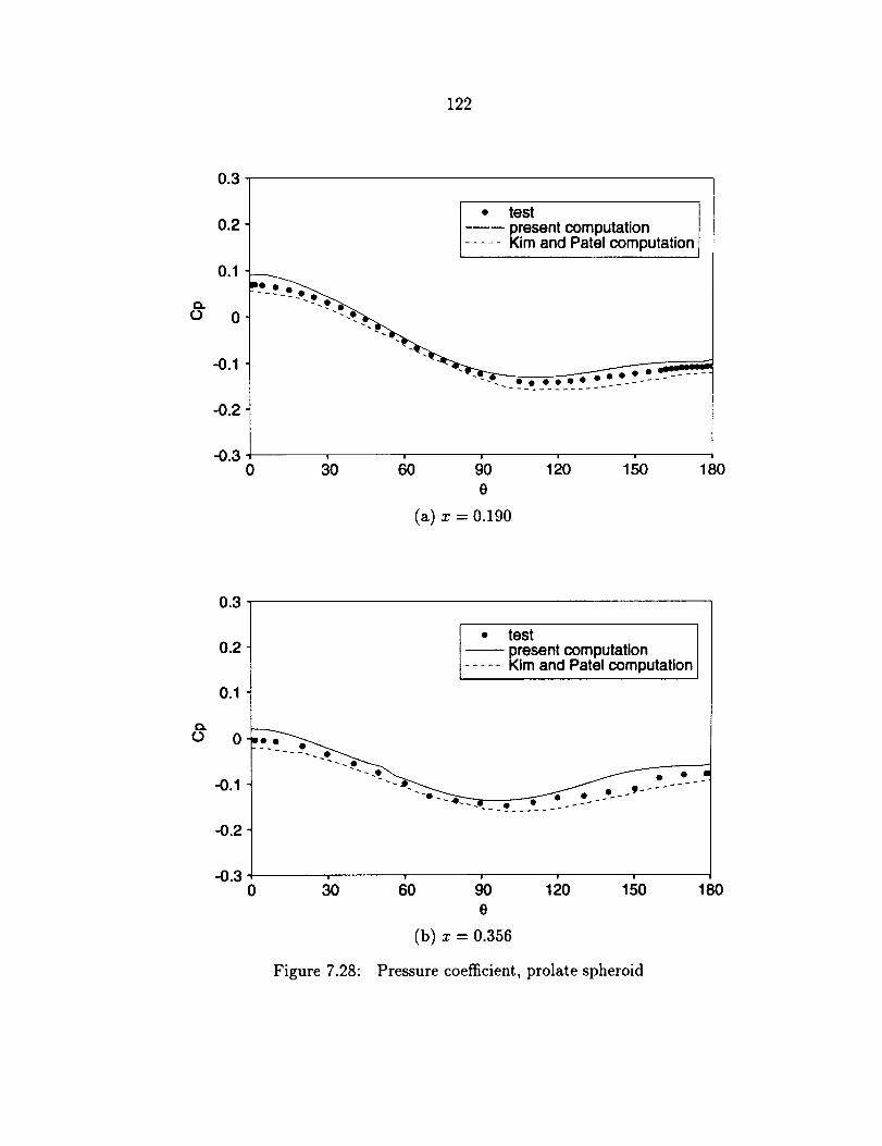
122

0.3

0.2

0.1

-0.2

-0.3

_____,__test 1present computationKim and Patel computation

0! ! i ! |

30 60 90 120 150

e

(a) x = 0.190

180

0.3

0.2

0.1

0.

-0.2

-0.3

__ • testpresent computation

--- Kim and Patel computation

i ! i I !

0 30 60 90 120 150 1800

(b) x = 0.356

Pressure coefficient, prolate spheroidFigure 7.28:

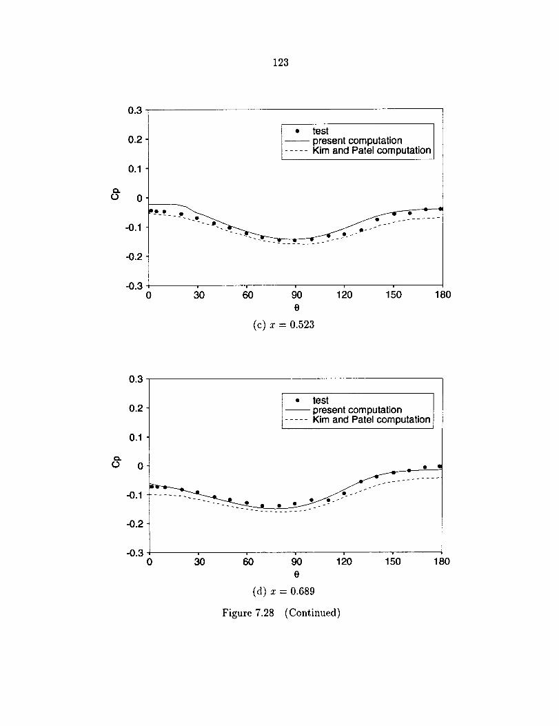
123

0.3

(3

0.2

0.1

0

-0.1

-0.2

-0.3

• test-- present computation..... Kim and Patel computation

' ' 9-0 ' '30 60 120 150

0

(c) x = 0.523

180

0.3

0.2

0.1

-0.2

-0.3

• test-- present computation..... Kim and Patel computation

0 30 90 120 150

8

(d) x = 0.689


180

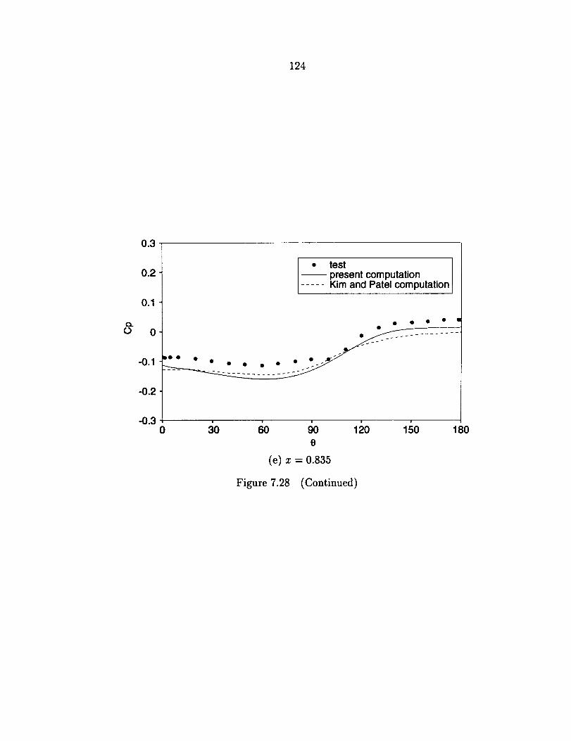
124

0.3

¢._

¢D

0.2

0.1

0

-0.1

-0.2

-0.3

___*__ testpresent computationKim and Patel computation

0 dO ' ' ' 15060 90 1200

(e) = = 0.835


180

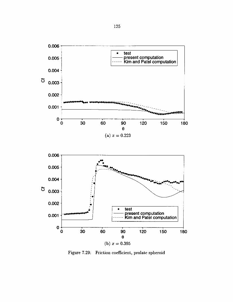
125

0.006

¢D

0.005

0.004

0.003

0.002

0.001

0

• test I-- present computation

Kim and Patel computation

0 30 60 90 120 150

0

(a) x = 0.223

180

0.006

0.005

0.004

0.003

0.002

0.001

0

Oi

!

0 30

Figure 7.29:

O _

We e

I • testpresent computation

..... Kim and Patel computation

w w u i

60 90 120 150

e

(b) x = 0.395

Friction coefficient, prolate spheroid

180

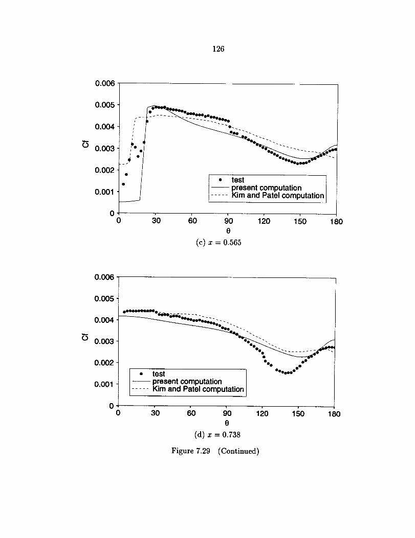
126

0.006

0.005

0.004

0.003

0,002

0,001

0

_O_ -

. - - _- - - - .... _ .... OeOOo_

," ] 1" test _ I/ I-- present.computation _ I

..... Kim and Patel computation tI

0i i ! ! !

30 60 90 120 150

0

(c) z = 0.565

180

0.006

0.005

0.004

0.003

0.002

0.001

0

O0 o O o°O

OOooooO• test-- present computation..... Kim and Patel computation

0 30 m v i I60 90 120 150e

(d) x = 0.738


180

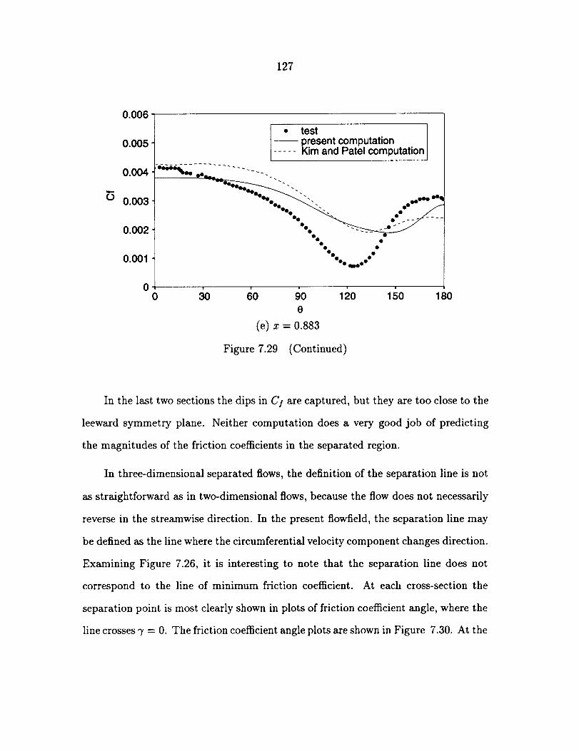
127

b

¢.)

0.006

0.005

0.004

0.003

0.002

0.001

0

• test-- present computation


ee _-el ' _ _ • _ - - _ - -

°°°Oo oo °

Oo o o •• me

o 8o 12o 18o8

(e) z = 0.883


In the last two sections the dips in C! are captured, but they are too close to the

leeward symmetry plane. Neither computation does a very good job of predicting

the magnitudes of the friction coefficients in the separated region.

In three-dimensional separated flows, the definition of the separation line is not

as straightforward as in two-dimensional flows, because the flow does not necessarily

reverse in the streamwise direction. In the present flowfield, the separation line may

be defined as the line where the circumferential velocity component changes direction.

Examining Figure 7.26, it is interesting to note that the separation line does not

correspond to the line of minimum friction coefficient. At each cross-section the

separation point is most clearly shown in plots of friction coefficient angle, where the

line crosses 7 = 0. The friction coefficient angle plots are shown in Figure 7.30. At the

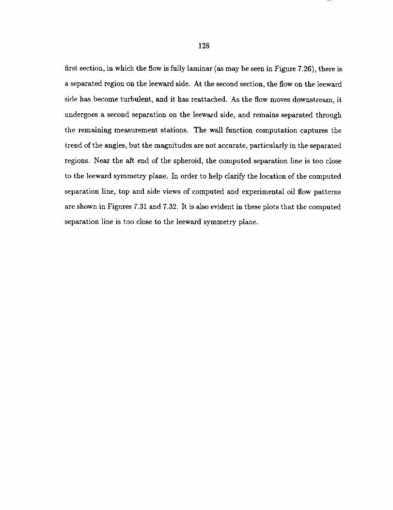
128

first section,in which the flow is fully laminar (asmaybeseenin Figure 7.26), there is

a separated region on the leeward side. At the second section, the flow on the leeward

side has become turbulent, and it has reattached. As the flow moves downstream, it

undergoes a second separation on the leeward side, and remains separated through

the remaining measurement stations. The wall function computation captures the

trend of the angles, but the magnitudes are not accurate, particularly in the separated

regions. Near the aft end of the spheroid, the computed separation line is too close

to the leeward symmetry plane. In order to help clarify the location of the computed

separation line, top and side views of computed and experimental oil flow patterns

are shown in Figures 7.31 and 7.32. It is also evident in these plots that the computed

separation line is too close to the leeward symmetry plane.

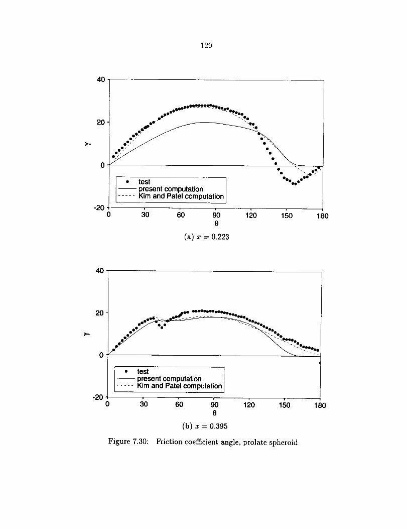
129

40

20

0

-20

" _

go - .._o.O°_"

OOo00ooO• test-- present computation..... Kim and Patel computation

0 30 do 90 _o _o 18oe

(a) x = 0.223

40

2O

0

-20

........ -,. _ ::_,........_/ - --..<.%.

•._ "_".,,..."" "0"._.°-o

/

• test t 1-- present computation I

- - Kim and Patel computation I r1e !o _o do 90 1_o _so 1so

(b) x = 0.395

Figure 7.30: Friction coefficient angle, prolate spheroid

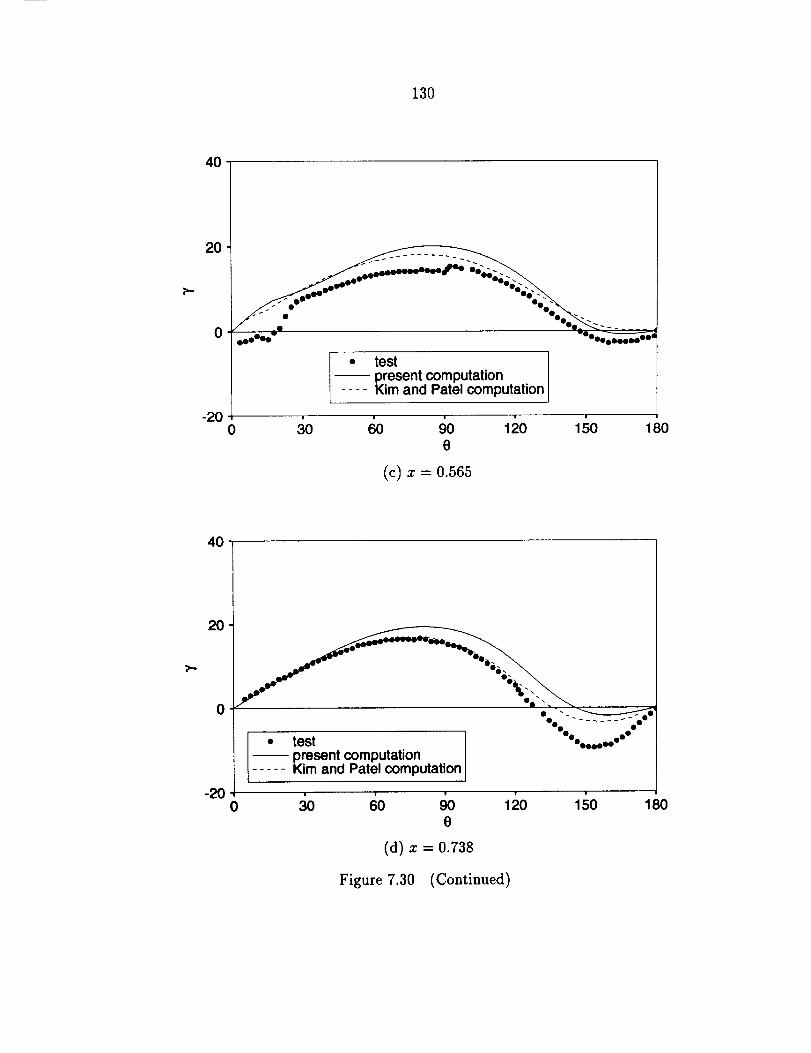
130

40

20

-20

I • test I- present computation

- - Kim and Patel computation

| !

0 30 60 90 1;)0 150

e

(c) z = 0.565

180

40

2O

p..

0

-2O

. ,es,-- present computation..... Kim and Patel computation

0 ' c;o _o ' '30 120 150 180e

(d) x = 0.738


131

40

2O

0

-20

test-- present computation


OOOOoo qboooOOOo0 O o° O0

O00_O0

0 ' ' ' 1:_0 '3O 60 90 150e

(e) x = 0.883


180

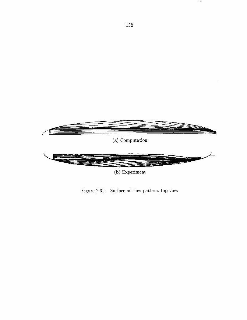
132

(a) Computation

(b) Experiment

Figure 7.31: Surface oil flow pattern, top view

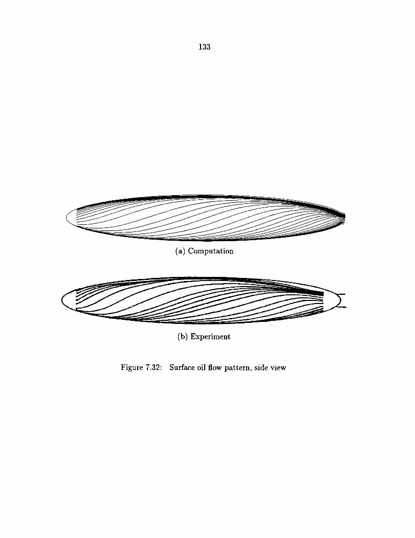
133

(a) Computation

(b) Experiment

Figure 7.32: Surface oil flow pattern, side view

135

8. CONCLUSIONS AND RECOMMENDATIONS

A method has been developed for the application of wall functions to generalized,

curvilinear, nonorthogonal grids. It has been applied to a series of test cases of vary-

ing complexity. Flat plate test cases were first run to check for coding errors and to

verify that the general formulation reduces correctly for this simple geometry. Com-

puted friction coefficients were in good agreement with values from a semi-empirical

equation. Since wall functions are based on the law of the wall, applicability of wall

functions to these test cases was not an issue.

The test cases for the body of revolution at zero angle of attack were more chal-

lenging. This flowfield had favorable and adverse pressure gradients and curvature of

the body surface. Pressure gradients were neglected in deriving the law of the wall,

and if they are large, they may cause inaccuracies in the shear stress calculation. The

standard k - e model is also known to be less accurate for flows with adverse pres-

sure gradients and/or strong streamline curvature (e.g., De Henneau, Raithby, and

Thompson 1990). Even with these limitations, it was shown that the wall function

formulation gave results comparable to the Baldwin-Lomax algebraic model and the

Chien low-Reynolds-number k - e model, all of which showed good agreement with

test data when using a relatively fine grid. One of the primary advantages of wall

functions is that they work well with coarse grid spacing, and this was also demon-

L_. INT_'.I!TlrtN_LI.y !,', ;, PRECEDING PAGE BLANK NOT FILMED

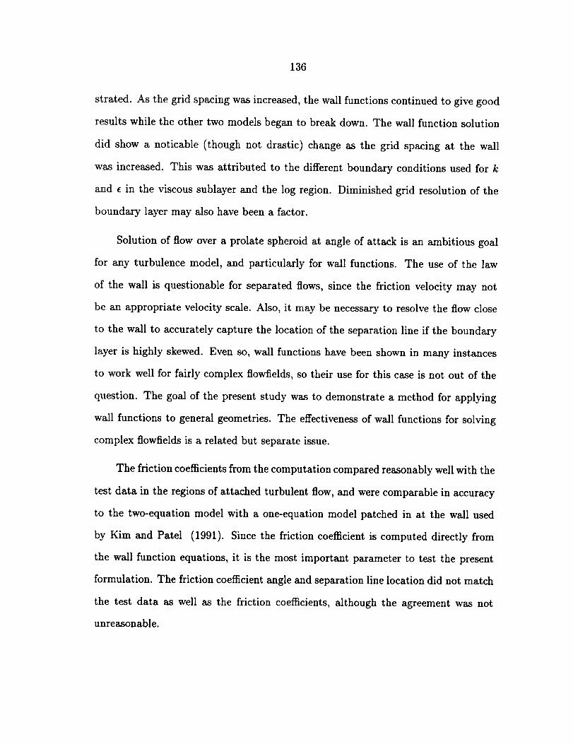
136

strated. As the grid spacing was increased, the wall functions continued to give good

results while the other two models began to break down. The wall function solution

did show a noticable (though not drastic) change as the grid spacing at the wall

was increased. This was attributed to the different boundary conditions used for k

and e in the viscous sublayer and the log region. Diminished grid resolution of the

boundary layer may also have been a factor.

Solution of flow over a prolate spheroid at angle of attack is an ambitious goal

for any turbulence model, and particularly for wall functions. The use of the law

of the wall is questionable for separated flows, since the friction velocity may not

be an appropriate velocity scale. Also, it may be necessary to resolve the flow close

to the wall to accurately capture the location of the separation line if the boundary

layer is highly skewed. Even so, wall functions have been shown in many instances

to work well for fairly complex flowfields, so their use for this case is not out of the

question. The goal of the present study was to demonstrate a method for applying

wall functions to general geometries. The effectiveness of wall functions for solving

complex flowfields is a related but separate issue.

The friction coefficients from the computation compared reasonably well with the

test data in the regions of attached turbulent flow, and were comparable in accuracy

to the two-equation model with a one-equation model patched in at the wall used

by Kim and Patel (1991). Since the friction coefficient is computed directly from

the wall function equations, it is the most important parameter to test the present

formulation. The friction coefficient angle and separation line location did not match

the test data as well as the friction coefficients, although the agreement was not

unreasonable.

137

The problem of resolving the boundary layer in the laminar regions of the flow-

field has several potential solutions. One is simply to use a finer grid. One of the

main reasons for using wall functions is to permit the use of coarser grids, thereby

saving grid points, so this solution is not ideal. A grid could be chosen which is a

compromise between the two requirements, however. Another solution would be to

use varying wall spacing. The wall spacing could be finer near the nose of the body

and gradually become coarser downstream. Alternatively, a separate grid with fine

wall spacing could be patched into the nose region. The flowfield could then be solved

using a grid-embedding technique such as chimera (Benek, Buning, and Steger 1985).

There are several improvements which should be investigated to improve the wall

function solution. It is possible to derive a modified law of the wall which accounts

for streamwise pressure gradients (Ferrari 1959). The application of this equation to

numerical schemes is not completely straightforward, since the equation takes on an

indeterminate form as the pressure gradient approaches zero. There is a well defined

limit at this point, however, so the problem should be surmountable. Although the

pressure gradient is usually neglected in standard wall function formulations, its effect

can be large (Mellor 1966; Tennekes and Lumley 1972), so the use of the modified law

of the wall should improve the solution for flows with significant pressure gradients.

It would be worthwhile to investigate this modification by solving a flowfield that is

simpler than the prolate spheroid at angle of attack. A separating boundary layer in

a two-dimensional diverging channel is a good choice.

A related possible improvement to the present formulation involves the applica-

tion of the computed shear stress to the right hand side of the Navier-Stokes equa-

tions. The shear stress at a point between the wall and the grid point adjacent to

138

the wall is presently assumedto equal the wall shearstress. If the boundary layer

assumption is invoked, the streamwisemomentum equation evaluated at the wall

yields the gradient of the shearstressasa function of streamwisepressuregradient.

A better estimate of the shear stressnear the wall is therefore possible. Although

the boundary layer assumption is not correct in someregionsof the flowfield, this

modification should still be an improvementover neglectingthe pressuregradient

altogether.

As mentioned above,the k - e model requires attention for flows with strong

adverse pressure gradients and streamline curvature. Various modifications have been

proposed (Launder, Priddin, and Sharma 1977; Hanjalic and Launder 1980; Rodi and

Scheuerer 1983; Pourahmadi and Humphrey 1983). Evaluation of these modifications

for relatively simple flowfields would be of value. The most promising formulation

could then be applied to the prolate spheroid problem. The use of wall functions

on curved surfaces should not pose any problems, since the law of the wall has been

observed to hold close to both convex and concave surfaces (Moser and Moin 1987).

Since neither the present computation nor the computation of Kim and Patel

(1991) gave accurate friction coefficients in the separated region of the flowfield (with

the exception of the middle measurement station in the present computation), the

problem may be in the k - e model itself, rather than the wall treatment. Diagnosing

this deficiency with the data available from the prolate spheroid measurements is

difficult. It would be useful to have a detailed set of turbulence measurements (e.g.

turbulent kinetic energy, Reynolds stress) available for a simpler separated flowfield

such as flow over an airfoil or flow in a diverging duct. Computing the flowfield using

139

avariety of turbulencemodelswould giveinsight into the specificdeficienciesof each

model.

141

9. REFERENCES

Abid, R., Speziale, C. G., and Thangam, S. (1991). "Application of a New K - T

Model to Near Wall Turbulent Flows." AIAA paper 91-0614, presented at 29th

Aerospace Sciences Meeting, Jan. 7-10, Reno, Nevada.

Anderson, D. A., Tannehill, J. C., and Pletcher, R. H. (1984). Computational Fluid

Mechanics and Heat Transfer. New York: McGraw-Hill.

Anton, H. A. (1973). Elementary Linear Algebra. New York: John Wiley & Sons.

Aris, R. (1962). Vectors, Tensors, and the Basic Equations of Fluid Mechanics.

Englewood Cliffs: Prentice-Hall.

Avva, R., Smith, C., and Singhal, A. (1990). "Comparative Study of High and Low

Reynolds Number Versions of k-e Models." AIAA paper 90-0246, presented at

the 28th Aerospace Sciences Meeting, Jan. 8-11, Reno, Nevada.

Baldwin, B. S. and Lomax, H. (1978). "Thin Layer Approximation and Algebraic

Model for Separated Turbulent Flows." AIAA paper 78-257, presented at the

16th Aerospace Sciences Meeting, Jan. 16-18, Huntsville, Alabama.

Benek, J. A., Buning, P. G., and Steger, J. L. (1985). "A 3-D Chimera Grid

Embedding Technique." AIAA paper 85-1523, presented at the 7th

Computational Fluid Dynamics Conference, July 15-17, Cincinnati, Ohio.

Bernard, P. S. (1986). "Limitations of the Near-Wall k-eps Turbulence Model."

AIAA Journal, 24, 619-622.

Cebeci, T. and Smith, A. M. O. (1974). Analysis of Turbulent Boundary Layers.

New York: Academic Press.

PRECED{NC, PAC,,,EBLAKq( NOT FIL&?ED

142

Chan, W. and Steger, J. (1991). "A Generalized Scheme for Three-Dimensional

Hyperbolic Grid Generation." AIAA paper 91-1588, presented at the 10th

Computational Fluid Dynamics Conference, June 24-26, Honolulu, Hawaii.

Chen, H. C. and Patel, V. C. (1987). "Practical Near-Wall Turbulence Models for

Complex Flows Including Separation." AIAA paper 87-1300, presented at the

19th Fluid Dynamics, Plasma Dynamics, and Lasers Conference, June 8-10,

Honolulu, Hawaii.

Chien, K.-Y. (1982). "Predictions of Channel and Boundary-Layer Flows with a

Low-Reynolds-Number Turbulence Model." AIAA Journal, 20, 33-38.

Chieng, C. C. and Launder, B. E. (1980). "On the Calculation of Turbulent Heat

Transport Downstream From an Abrupt Pipe Expansion." Numerical Heat

Transfer, 3, 189-207.

Chou, P.Y. (1945). "On Velocity Correlations and the Solutions of the Equations

of Turbulent Fluctuation." Quarterly of Applied Mathematics, 3, 38-54.

Coakley, T. J. (1983). "Turbulence Modeling Methods for the Compressible

Navier-Stokes Equations." AIAA paper 83-1693, presented at the 16th Fluid

and Plasma Dynamics Conference, July 12-14, Danvers, Mass.

Coles, D. E. (1956). "The Law of the Wake in the Turbulent Boundary Layer."

Journal of Fluid Mechanics, 1, 191-226.

Coles, D. E. and Hirst, E. A., ed. (1969). Proceedings, Computation of Turbulent

Boundary Layers- 1968 AFOSR-IFP-Stanford Conference. Vol. II, Compiled

Data. Palo Alto: Thermosciences Division, Department of Mechanical

Engineering, Stanford University.

Daly, B. J. and Harlow, F. H. (1970). "Transport Equations in Turbulence." The

Physics of Fluids, 13, 2634-2649.

De Henneau, V., Raithby, G. D., and Thompson, B. E. (1990). "Prediction of

Flows with Strong Curvature and Pressure Gradient using the k -

Turbulence Model." ASME Journal of Fluid Mechanics, 112, 40-47.

143

Deng, G. B., Piquet, J., and Queutey,P. (1990). "Navier-StokesComputations ofVortical Flows." AIAA paper90-1628,presentedat the 21st Fluid Dynamics,Plasma Dynamics,and LasersConference,Aug. 17-19,Seattle,Wa.

El Tahry, S. H. (1983). "k - e Equation for Compressible Reciprocating Engine

Flows." Journal of Energy, 7, no. 4, 345-353.

Ferrari, C. (1959). "Wall Turbulence." NASA Republication 2-8-59W, translation

of Section C of the monograph entitled "Corso sulla Teoria della Turbolenza,"

from lectures delivered at the International Center of Mathematical Summer

Studies (C.I.M.E.), Sept. 1-10, Varenna, Italy.

Ferziger, J. H. (1987). "Simulation of Incompressible Turbulent Flows." Journal of

Computational Physics, 69, 1-48.

Gibson, M. M., Jones, W. P., and Younis, B. A. (1981). "Calculation of Turbulent

Boundary Layers on Curved Surfaces." The Physics of Fluids, 24, 386-395.

Gorski, J. J. (1984). "A New Near-Wall Formulation for the k - e Equations of

Turbulence." AIAA paper 86-0556, presented at 24th Aerospace Sciences

Meeting, Jan. 6-9, Reno, Nevada.

Hanjalic, K. and Launder, B. E. (1980). "Sensitizing the Dissipation Equation to

Irrotational Strains." ASME Journal of Fluids Engineering, 102, 34-40.

Harlow, F. H. and Nakayama, P. I. (1967). "Turbulence Transport Equations."

The Physics of Fluids, 10, 2323-2332.

Harlow, F. H. and Nakayama, P. I. (1968). "Transport of Turbulence Energy

Decay Rate." Los Alamos: Los Alamos Scientific Laboratory. Report LA-3854.

Hinze, J. O. (1987). Turbulence. 2nd ed. McGraw-Hill Classic Textbook Reissue

Series. New York: McGraw-Hill.

Hornbeck, R.W. (1975). Numerical Methods. New York: Quantum Publishers.

Jones, W. P. and Launder, B. E. (1972). "The Prediction of Laminarization With

a Two-Equation Model of Turbulence." International Journal of Heat Transfer,

15, 301-314.

144

K_Lylla_, 0. _md Florcs, J. (1987). "A(hCm(:(_s in the Computation of Transonic

Separ_t, ed Flows over Finite Wings." AIAA Impcr 87-1195, prt_entcd at the

19th Fhfid Dymnni(:s, Pbhsma Dynamics _md L_L,_;rs Confi;rcn(:(,, June 8-10,

Honohflu, H_tw_di.

Kim, S. E. ,rod P_ttel, V. C. (1991). "Separ,Ltion on a Spheroid _.t In('idenee:

Turlmlent Flow." In P_w:eedings of the Second Osaka Inteywational Colhutuium

on Viscou,_' Fluid Dynamics in Ship and Oa;an Technology, Osaka, Jalgm IW

Osalm University. Osalo_: Osaka University, 1-25.

Kim, S.-W. and Chen. C.-P. (1989). "A Multiph_TiIKu.,-S(:,dc Turtmh,n(:c Model

Ba.s('(1 on Varialfl(', P_rtitioning of th(, qSlrbulent Kin(;ti(: En(;rgy Sp(;(:trmn."

Numerical Heat Ttunsfi;r, P_rt B, 16, 193-211.

Kleb_moff. P. S. (1955). "Charax:tcristics of qSlrbuh;nee in a Boundary L_wer with

Zero Pres,surc Gr_uli(;nt." W_Lshington, D.C.: N_tionM Advisor3: Committ(w fi}r

Aeronmlti(:s. NACA Report 1247.

Ko, S. H. _m(1 Rhode, D. L. (1990). "Derivation and T(;sting of a New Multi-S(:alc

k - _. rlSlrbul(.'ncc Model." AIAA p_q)cr 90-1243, presented at, tim 28th

Aerospa_:c Sciences M(,cting, J_m. 8-11, Pw.no, Ncv_ula.

Kreplin, H.-P., Meier, H. U., and M,ficr A. (1978). "Wind qSmnel Model and

M(;a_uring Techniques fi}r the Im, cstigation of Thrc¢.,-Dimcnsi(mal Turbulent

Boun(tmT L_ycrs." In Pnx.vedings of the AIAA IOth Aem. Testing Confi'n:nce,

San Diego, Ca., by the Amerie_m Institute of Aeronautics and Astronmlti(:s.

W_Lshington, D.C.: Ameri('_m Institute of Aeronautics _m(l Astr(mauti(:s, 93-97.

Kreplin, H.-P., Volhtwrs. H., and Meier, H. U. (1982). "Mcm4urcmcnts of the Wall

Sh(,ax Stres_s on asi Inclined Prolatc Spheroid." Zeitsch_ifl fur Flugwissenschaft

Welt_umttfo_schun9, 6, 248-252.

Launder, B. E. (1979). "Reynolds Str{_ss Ch_sur_s - Status aaul Pr(mpc(:t_." in

7)_rbulent Boundary Layen_ - Ezw_irnents , Theo_l and M_Melliny: P_r_:cedinys

of the 45th Panel Meeting/Symlm.s_um hem in The Hague, Netherlands, Sept.

24-28, by the. A(Lf_)r3, Group fi)r A(:r_xsp_u:e Rx.,se_m:h and Dcvc, lopincnt.

AGARD Confi:ren(:e Proee_._lings No. 271. Neuilly sur Seine: the Advisory

Group fi}r Aerospace Rx;se_r<:h and Development. 13-1-13-13.

Launder, B. E. (1984). "Second-Moment Closure: Methodology mid Practice." in

Turbulena" MtuleL_ and their Applications., vol. 2, P_is: Editions Eyrolh;s.

145

Launder, B. E., Morse,A., Rodi, W., and Spalding,D. B. (1972). "Prediction ofFreeShearFlows--A Comparisonof the Performanceof Six TurbulenceModels." in Free Turbulent Shear Flows: Proceedings of a conference held at

NASA Langley Research Center, Hampton, Va., July 20-21, by the National

Aeronautics and Space Administration. NASA SP-321. Washington, D.C.:

National Aeronautics and Space Administration. 361-426.

Launder, B. E. and Spalding, D. B. (1974). "The Numerical Computation of

Turbulent Flows." Computer Methods in Applied Mechanics and Engineering,

3, 269-289.

Launder, B. E., Priddin, C. H., and Sharma, B. I. (1977). "The Calculation of

Turbulent Boundary Layers on Spinning and Curved Surfaces." ASME Journal

of Fluids Engineering, 99, 231-239.

Lewis, J. P. and Pletcher, R. H. (1986). "A Boundary-Layer Computational Model

for Predicting the Flow and Heat Transfer in Sudden Expansions." Ames: Iowa

State University College of Engineering. Technical Report HTL-41, CFD-14.

Mansour, N. N., Kim, J., and Moin, P. (1989). "Near-Wall k - e Turbulence

Modeling." AIAA Journal, 27, 1068-1073.

Meier, H. U. and Kreplin, H.-P. (1979). "Experimental Investigation of the

Transition and Separation Phenomena on a Body of Revolution." Proceedings

of the 2nd Symposium on Turbulent Shear Flows, London, England, July 2-4,

1979. London: Imperial College of Science and Technology, 15.1-15.7.

Meier, H. U. and Kreplin, H.-P. (1980). "Experimental Investigation of the

Boundary Layer Transition and Separation on a Body of Revolution."

Zeitschrift fur Flugwissenschaft Weltraumforschung, 4, 65-71.

Meier, H. U., Kreplin, H.-P., and Vollmers, H. (1983). "Development of Boundary

Layers and Separation Patterns on a Body of Revolution at Incidence."

Proceedings of the 2nd Symposium on Numerical and Physical Aspects of

Aerodynamic Flows, Long Beach, Ca., Jan. 17-20, by California State

University at Long Beach. Long Beach: California State University, 1-9.

Mellor, G. L. (1966). "The Effects of Pressure Gradients on Turbulent Flow Near a

Smooth Wall." Journal of Fluid Mechanics, 24, 255-274.

146

Michelassi, V. and Shih, T.-H. (1991). Low Reynolds Number Two-Equation

Modeling of Turbulent Flows." Washington, D. C.: National Aeronautics and

Space Administration. NASA TM-104368.

Monin, A. S. and Yaglom, A. M. (1987). Statistical Fluid Mechanics: Mechanics of

Turbulence. vol. 1. Cambridge: The MIT Press.

Moser, R. D. and Moin, P. (1987). "The Effects of Curvature in Wall-Bounded

Turbulent Flows." Journal of Fluid Mechanics, 175, 479-510.

Norris, H. L. and Reynolds, W. C. (1975). "Turbulent Channel Flow with a

Moving Wavy Boundary." Stanford: Stanford University. Department of

Mechanical Engineering Technical Report TF-7.

Pan, D. and Pulliam, T. H. (1986). "The Computation of Steady 3-D Separated

Flows Over Aerodynamic Bodies at Incidence and Yaw." AIAA paper 86-0109,

presented at the 24th Aerospace Sciences Meeting, Jan. 6-9, Reno, Nevada.

Panaras, A. G. and Steger, J. L. (1988). "A Thin-Layer Solution of the Flow about

a Prolate Spheroid." Zeitschrift fur Flugwissenschaf't Weltraumforschung, 12,173-180.

Patankar, S. V. and Spalding, D. B. (1970). Heat and Mass Transfer in BoundaryLayers. 2nd ed. London: Intertext Books.

Patel, V. P., Rodi, W., and Scheuerer, G. (1985). "Turbulence Models for

Near-Wall and Low Reynolds Number Flows: A Review." AIAA Journal, 23,1308-1319.

Peterson, V. L., Kim, J., Holst, T. L., Diewert, G. S., Cooper, D. M., Watson, A.

B., and Bailey, F. R. (1989). "Supercomputer Requirements for Selected

Disciplines Important to Aerospace." Journal of LE.E.E., 77.

Pourahmadi, F. and Humphrey, A. C. (1983). "Prediction of Curved Channel Flow

with an Extended k - e Model of Turbulence." AIAA Journal, 21, 1365-1373.

Pulliam, T. H. (1984). "Euler and Thin Layer Navier-Stokes Codes: ARC2D,

ARC3D." notes for Computational Fluid Dynamics User's Workshop held at

The University of Tennesee Space Institute, Tullahoma, Tennessee, March

i2-16. Tullahoma: University of Tennesee Space Institute. Photocopied.

147

Pulliam, T. H. (1985). "Artificial Dissipation Models for the Euler Equations."AIAA paper 85-0438,presentedat the 23rd AerospaceSciencesMeeting, Jan.14-17,Reno, Nevada.

Rai, M. M. and Moin, P. (1989). 'Direct Simulationsof Turbulent Flow usingFinite-Difference Schemes."AIAA paper 89-0369,presentedat the 27thAerospaceSciencesMeeting, Jan. 9-12,Reno,Nevada.

Ramaprian, B. R., Patel, V. C., and Choi, D. H. (1978). Mean Flow Measurements

in the Three-Dimensional Boundary Layer over a Body of Revolution at

Incidence. Iowa City: Iowa Institute of Hydraulic Research, The University of

Iowa. IIHR Limited Distribution Report No. 56.

Ramaprian, B. R., Patel, V. C., and Choi, D. H. (1981). "Mean Flow

Measurements in the Three-Dimensional Boundary Layer over a Body of

Revolution at Incidence." Journal of Fluid Mechanics, 103, 479-504.

Reynolds, O. (1895). "On the Dynamical Theory of Incompressible Viscous Fluids

and the Determination of the Criterion." Philosophical Transactions of the

Royal Society of London, 186, Series A, 123-164.

Rodi, W. (1972). "The Prediction of Free Turbulent Boundary Layers by the Use of

a Two-Equation Model of Turbulence." Ph.D. thesis, Imperial College, London.

Rodi, W. (1980). Turbulence Models and their Application in Hydraulics -- A State

of the Art Review. Delft: International Association for Hydraulic Research.

Rodi, W. (1991). "Experience with Two-Layer Models Combining the k - e Model

with a One-Equation Model Near the Wall." AIAA paper 91-0216, presented at

the 29th Aerospace Sciences Meeting, Jan. 7-10, Reno, Nevada.

Rodi, W. and Scheuerer, G. (1983). "Calculation of Curved Shear Layers with

Two-Equation Turbulence Models." Physics of Fluids, 26, 1422-1436.

Rodi, W. and Spalding, D. B. (1970). "A Two-Parameter Model of Turbulence,

and its Application to Free Jets." Warme-und Stoffubertragung, 3, 85-95.

Schetz, J. A. (1980). Injection and Mixing in Turbulent Flow. New York:

American Institute of Aeronautics and Astronautics.

Schlichting, H. (1984). Boundary-Layer Theory. 7th ed. New York: McGraw-Hill.

148

Shih, T. H. and Mansour,N. N. (1990). "Modeling of Near-Wall Turbulence." inProceedings of the CFD Symposium on Aeropropulsion at the NASA Lewis

Research Center in Cleveland, Ohio, Apr. 2_-26, by the National Aeronautics

and Space Administration. Washington, D.C.: National Aeronautics and Space

Administration, 1-11.

Shih, T. H. and Hsu, A. T. (1991). "An Improved k - e Model for Near-Wall

Turbulence." AIAA paper 91-0611, presented at the 29th Aerospace Sciences

Meeting, Jan. 7-10, Reno, Nevada.

Shih, T. I.-P. and Chyu, W. J. (1991). "Approximate Factorization with Source

Terms." AIAA Journal, 29, 1759-1760.

Sokolnikoff, I. S. (1964). Tensor Analysis Theory and Applications to Geometry

and Mechanics of Continua. 2nd ed. New York: John Wiley & Sons.

Speziale, C. G. (1987). "On Nonlinear K - l and K - e Models of Turbulence."

Journal of FLuid Mechanics, 178, 459-475.

Steger, J. L. and Warming, R. F. (1981). "Flux Vector Splitting of the Inviscid

Gasdynamic Equations with Application to Finite-Difference Methods."

Journal of Computational Physics, 40, 263-293.

Taylor, G. I. (1935). "Statistical Theory of Turbulence." Proceedings of the Royal

Society of London, 151A, 421-478.

Tennekes, H. and Lumley, J. L. (1972). A First Course in Turbulence. Cambridge:

The MIT Press.

Van Driest, E. R. (1956). "On Turbulent Flow Near a Wall." Journal of the

Aeronautical Sciences, 23, 1007-1011, 1036.

Vatsa, V. N., Thomas, J. L., and Wedan, B.W. (1987). "Navier-Stokes

Computations of Prolate Spheroids at Angle of Attack." AIAA paper 87-2627,

presented at the Atmospheric Flight Mechanics Conference, Aug. 17-19,

Monterey, Ca.

Viegas, J. R. and Rubesin, M. W. (1983). "Wall-Function Boundary Conditions in

the Solution of the Navier-Stokes Equations for Complex Compressible Flows."

AIAA paper 83-1694, presented at the 16th Fluid and Plasma Dynamics

Conference, July 12-14, Dancers, Mass.

149

Viegas, J. R., Rubesin, M. W., and Horstman, C. C. (1985). "On the Use of Wall

Functions as Boundary Conditions for Two-Dimensional Separated

Compressible Flows." AIAA paper 85-0180, presented at the 23rd Aerospace

Sciences Meeting, Jan. 14-17, Reno, Nevada.

White, F. M. (1974). Viscous Fluid Flow. New York: McGraw-Hill.

Wilcox, D. C. (1988). "Reassessment of the Scale-Determining Equation for

Advanced Turbulence Models." AIAA Journal, 26, 1299-1310.

Wong, T.-C., Kandil, O. A., and Liu, C. H. (1989). "Navier-Stokes Computations

of Separated Vortical Flows Past Prolate Spheroid at Incidence." AIAA paper

89-0553, presented at the 27th Aerospace Sciences Meeting, Jan. 9-12, Reno,Nevada.

Yakhot, V. and Orszag, S. A. (1986). "Renormalization Group Analysis of

Turbulence. I. Basic Theory." Journal of Scientific Computing, 1, 3-51.

Ying, S. X., Steger, J. L., Schiff, L. B., and Baganoff, D. (1986). "Numerical

Simulation of Unsteady, Viscous, High-Angle-of-Attack Flows Using a Partially

Flux-Split Algorithm." AIAA paper 86-2179, presented at the 13th

Atmospheric Flight Mechanics Conference, Aug. 18-20, Williamsburg, Virginia.

Yoshizawa, A. (1988). "Statistical Modelling of Passive-Scalar Diffusion in

Turbulent Shear Flows." Journal of Fluid Mechanics, 195,541-555.

,z)

151

10. APPENDIX A: FLUX JACOBIANS

I0.I Navier-Stokes

Before presenting these matrices, a word about their derivation is in order. Each

flux vector may be considered to be a function of both the dependent variable vector

Q and its spatial derivatives, for example OQ/Ox. We may therefore write for a

one-dimensional equation

AOE

oQOE(Q, Q_) aE(Q, Q_) OQ:_

- +OQ aQ= OQ

(i0.i)

It is common practice to neglect the second term on the right hand side (e.g. Pulliam

1984), and this approximation will be made here. Using the notation of Pulliam, the

Jacobian matrices are as follows.

PI:_CEDING PAGE BLANK NOT FILMED

152

A

_t

-u0 + _¢2

-w0 + _¢2

0 [¢2_ el]

_,+0-(7- 2)_u

_v- (7- 1)6u

4_w- (7- 1)_zu

4_al - (7- 1)u0

_vu - (7 - 1)_.v

_,+o-(7- 2)_v

_,,, - (7 - 1)_zv

_al - (7 -- 1)v0

where

_u - (7 - 1),_w (7 - l),,c_

,,C:v- (7 - 1),,C_w (,.),-1)6

,Ct+ 8 - ("),- 2),,C:w (7 - 1),,c_

_al - (7- 1)wO 7O+ _,

(10.2)

7C ¢_a, - (10.3)P

8 = _u + _v + ,_w (10.4)

¢2 1= _ (7- 1)(u2 + v2 + w 2) (10.5)

The flux Jacobians B and C are identical to the above matrix, with the exception

that all occurrences of _ are replaced with 7/or _ respectively.

The viscous Jacobian, neglecting cross-derivative terms, is

0 0 0 0 0

o

rn51 m52 rn53 rnM m55

v .__ (10.6)

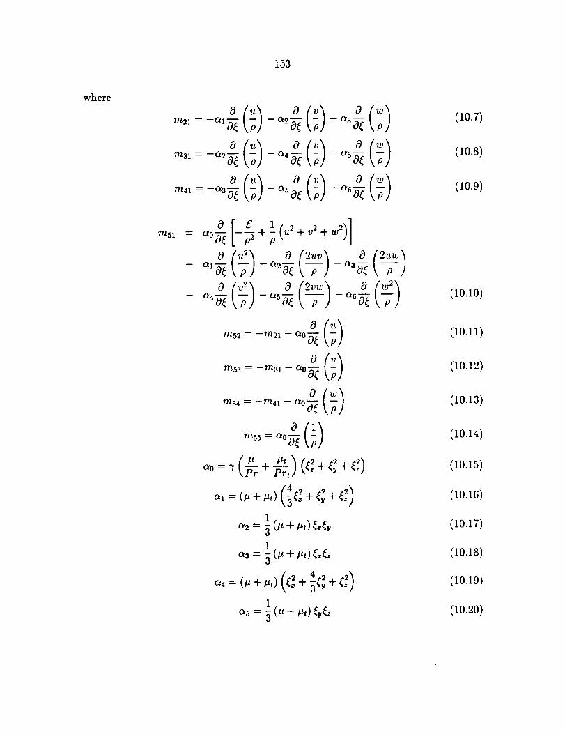
153

where

o(:)m51 [_ 1 v2 )]o__ ;_o_ + (u2+ +w2

_1_ - _ -_

o °(V)- °

m53 "- --7T/31 -- (_0_-_

m54 ---- --m41 -- ao_- _

m55 _- OLO_'_

_o=_ _ + _-_, _+

I

1

43 = 5(,+ i..) _._.

42 (2)_4 = (_,+ _,,)(_ + _ +

1_ = _(_,+ _,)_,

(lO.7)

(10.8)

(10.9)

(10.10)

(10.11)

(10.12)

(10.13)

(10.14)

(10.15)

(10.16)

(10.17)

(10.18)

(10.19)

(10.20)

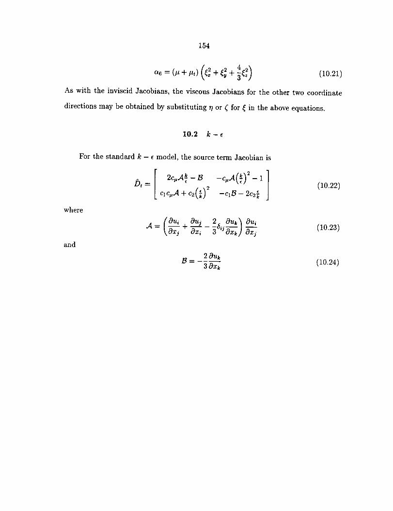
154

As with the inviscid Jacobians, the viscous Jacobians for the other two coordinate

directions may be obtained by substituting _ or _ for _ in the above equations.

10.2 k - e

where

and

For the standard k - e model, the source term Jacobian is

b, = c,c._+c2(_)2 -c1_- 2c2_(10.22)

2 0uk (10.24)30x_:

(ou, out 2_ Ou_ ou, (10.23).A- _kOxj + Oxi 3 iJ_xk/ _xj

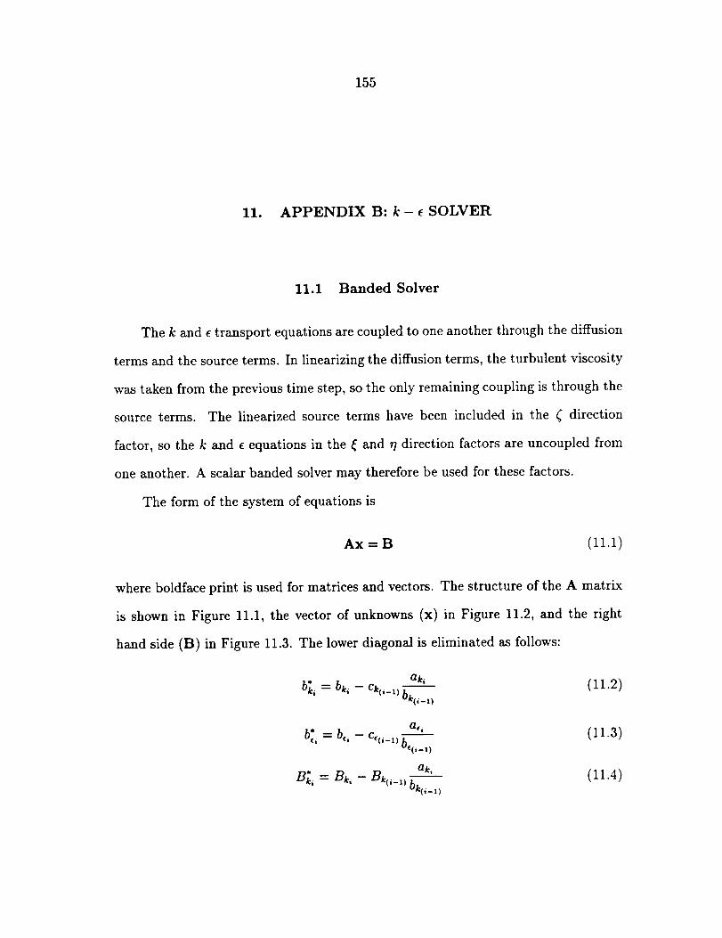
155

11. APPENDIX B: k-e SOLVER

11.1 Banded Solver

The k and e transport equations are coupled to one another through the diffusion

terms and the source terms. In linearizing the diffusion terms, the turbulent viscosity

was taken from the previous time step, so the only remaining coupling is through the

source terms. The linearized source terms have been included in the _ direction

factor, so the k and e equations in the _ and rI direction factors are uncoupled from

one another. A scalar banded solver may therefore be used for these factors.

The form of the system of equations is

Ax = B (11.1)

where boldface print is used for matrices and vectors. The structure of the A matrix

is shown in Figure 11.1, the vector of unknowns (x) in Figure 11.2, and the right

ak, (11.2)b" = bk,k, -- Cko-_) bk(___)

b* =b,, - a_, (11.3)

ak, (11.4)B_, = Bk, - B_(,_,)bk(,_,)

hand side (B) in Figure 11.3. The lower diagonal is eliminated as follows:

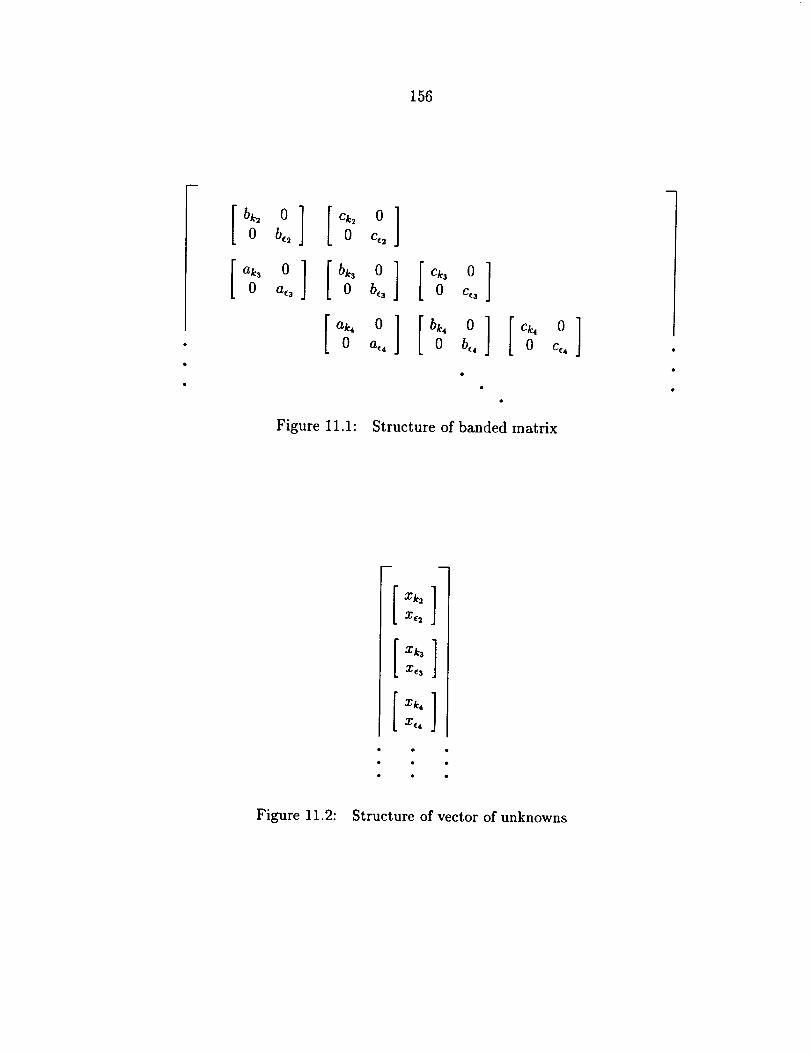
156

bk20

ak30

0 0

0 ce2

0 0

0 Cc3

O] 00 at4 0 be4] [ ck40

Figure 11.1:

0

C_ 4

Structure of banded matrix

m

X_ 2

X_3

X_ 4

Figure 11.2: Structure of vector of unknowns

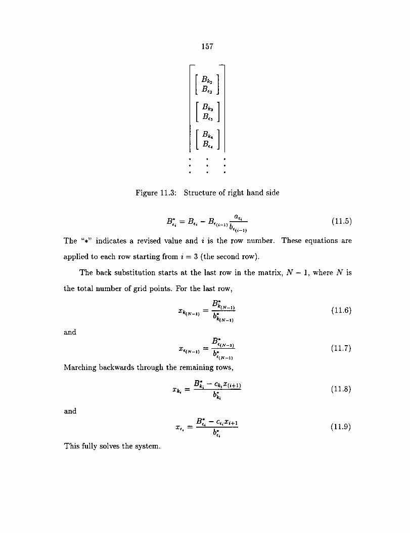
157

m

Bk2B,2 ]

B_3

[Bk,B. ]

Figure 11.3: Structure of right hand side

ac i

B2, = B,, - B_(,_,)b_(,_,)

The "*" indicates a revised value and i is the row number.

applied to each row starting from i = 3 (the second row).

(11.5)

These equations are

and

the total number of grid points. For the last row,

B_(N_,)

Xk(N_I)- b*k(N_l)

B_(N-1)

X_(N_a ) -- b_(N_l )

Marching backwards through the remaining rows,

(11.6)

(11.7)

bi,(11.8)

and

X_ i --*

B_i - CeiXi+ 1

b_,(11.9)

This fully solves the system.

The back substitution starts at the last row in the matrix, N - 1, where N is

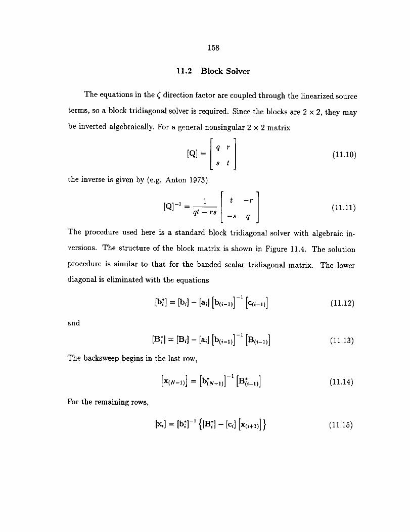
158

11.2 Block Solver

The equations in the ¢ direction factor are coupled through the linearized source

terms, so a block tridiagonal solver is required. Since the blocks are 2 x 2, they may

be inverted algebraically. For a general nonsingular 2 x 2 matrix

[q] =

the inverse is given by (e.g. Anton 1973)

q r

s t(11.10)

[Q]-I _ 1 t -r (11.11)qt - rs

-s q

The procedure used here is a standard block tridiagonal solver with algebraic in-

versions. The structure of the block matrix is shown in Figure 11.4. The solution

procedure is similar to that for the banded scalar tridiagonal matrix. The lower

diagonal is eliminated with the equations

and

rB_j=IB,j-Ea,][b_,_,,]-'[B_,_,_]The backsweep begins in the last row,

[x,__,,]_-[_;__,,]-'[_:,__,]

For the remaining rows,

(11.12)

(11.13)

(11.14)

[x,] = [b_] -1 {[B_]- [c,] [x0+,)] } (11.15)

159

[b2] [c2] 1[a3] [b3] [c3]

[a4] [b4] [c4]

Figure 11.4: Structure of block matrix

Documents

neering - NASA · Skewed flat plate grid ..... 82 Friction coefficient, flat plate, skewed grid ..... 83 Velocity profile, flat plate, skewed grid ..... 84 Friction coefficient,