NPS-OC-09-006

NAVAL POSTGRADUATE

SCHOOL

MONTEREY, CALIFORNIA

Approved for public release; distribution is unlimited.

Prepared for: CNO(N45), Washington, D.C.

Marine Mammal Acoustic Monitoring and Habitat Investigation, Southern California Offshore Region

by

John Hildebrand

June 2009

THIS PAGE INTENTIONALLY LEFT BLANK

NAVAL POSTGRADUATE SCHOOL

Monterey, California 93943-5000 Daniel T. Oliver Leonard A. Ferrari President Executive Vice President and Provost This report was prepared for CNO(N45), Washington, D.C. and funded by CNO(N45), Washington, D.C. Reproduction of all or part of this report is authorized. This report was prepared by: ________________________ John Hildebrand Professor of Oceanography Scripps Institution of Oceanography Reviewed by: Released by: ________________________ ______________________________ Jeffrey Paduan Karl Van Bibber Department of Oceanography Vice President and Dean of Research

THIS PAGE INTENTIONALLY LEFT BLANK

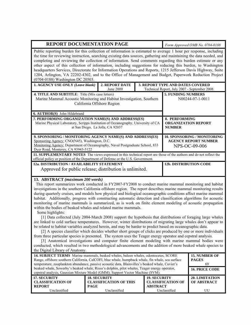
REPORT DOCUMENTATION PAGE Form Approved OMB No. 0704-0188 Public reporting burden for this collection of information is estimated to average 1 hour per response, including the time for reviewing instruction, searching existing data sources, gathering and maintaining the data needed, and completing and reviewing the collection of information. Send comments regarding this burden estimate or any other aspect of this collection of information, including suggestions for reducing this burden, to Washington headquarters Services, Directorate for Information Operations and Reports, 1215 Jefferson Davis Highway, Suite 1204, Arlington, VA 22202-4302, and to the Office of Management and Budget, Paperwork Reduction Project (0704-0188) Washington DC 20503. 1. AGENCY USE ONLY (Leave blank)

2. REPORT DATE June 2009

3. REPORT TYPE AND DATES COVERED Technical Report, July 2007 - September 2008

4. TITLE AND SUBTITLE: Title (Mix case letters) Marine Mammal Acoustic Monitoring and Habitat Investigation, Southern

California Offshore Region

6. AUTHOR(S) John Hildebrand

5. FUNDING NUMBERS N00244-07-1-0011

7. PERFORMING ORGANIZATION NAME(S) AND ADDRESS(ES) Marine Physical Laboratory, Scripps Institution of Oceanography, University of CA

at San Diego, La Jolla, CA 92037

8. PERFORMING ORGANIZATION REPORT NUMBER

9. SPONSORING / MONITORING AGENCY NAME(S) AND ADDRESS(ES) Sponsoring Agency: CNO(N45), Washington, D.C. Monitoring Agency: Department of Oceanography, Naval Postgraduate School, 833 Dyer Road, Monterey, CA 93943-5122

10. SPONSORING / MONITORING AGENCY REPORT NUMBER

NPS-OC-09-006

11. SUPPLEMENTARY NOTES The views expressed in this technical report are those of the authors and do not reflect the official policy or position of the Department of Defense or the U.S. Government.

12a. DISTRIBUTION / AVAILABILITY STATEMENT

Approved for public release; distribution is unlimited.

12b. DISTRIBUTION CODE

13. ABSTRACT (maximum 200 words) This report summarizes work conducted in FY2007-FY2008 to conduct marine mammal monitoring and habitat investigations in the southern California offshore region. The report describes marine mammal monitoring results during quarterly cruises, and models how physical and biological oceanographic conditions affect marine mammal habitat. Additionally, progress with constructing automatic detection and classification algorithms for acoustic monitoring of marine mammals is summarized, as is work on finite element modeling of acoustic propagation within the bodies of beaked whales and related marine mammals. Some highlights: [1] Data collected (July 2004-March 2008) support the hypothesis that distributions of foraging large whales are linked to cold surface temperatures. However, winter distributions of migrating large whales don’t appear to be related to habitat variables analyzed herein, and may be harder to predict based on oceanographic data. [2] A species classifier which decides whether short groups of clicks are produced by one or more individuals from three particular species is presented. The system uses the Teager energy operator and cepstral analysis. [3] Anatomical investigations and computer finite element modeling with marine mammal bodies were conducted, which resulted in two methodological advancements and the addition of more beaked whale species to the Digital Library of Anatomy.

15. NUMBER OF PAGES

69

14. SUBJECT TERMS Marine mammals, beaked whales, baleen whales, odontocetes, SCORE Range, offshore southern California, CalCOFI, blue whale, humpback whale, fin whale, sea surface temperature, zooplankton abundance, passive acoustic data, Blainvilles’s beaked whale, Cuvier’s beaked whale, Sowerby’s beaked whale, Risso’s dolphin, pilot whales, Teager energy operator, cepstral analysis, Gaussian Mixture Model (GMM), Support Vector Machine (SVM).

16. PRICE CODE

17. SECURITY CLASSIFICATION OF REPORT

Unclassified

18. SECURITY CLASSIFICATION OF THIS PAGE

Unclassified

19. SECURITY CLASSIFICATION OF ABSTRACT

Unclassified

20. LIMITATION OF ABSTRACT

UU

THIS PAGE INTENTIONALLY LEFT BLANK

i

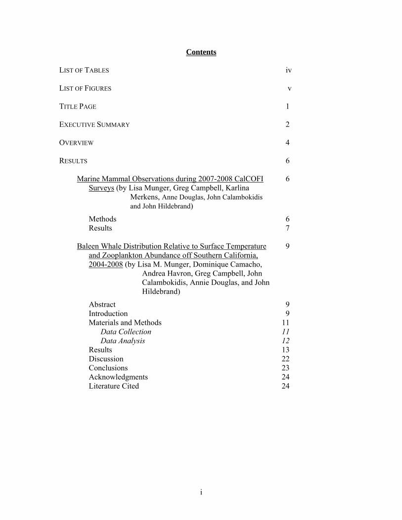
Contents LIST OF TABLES LIST OF FIGURES TITLE PAGE EXECUTIVE SUMMARY OVERVIEW RESULTS

Marine Mammal Observations during 2007-2008 CalCOFI Surveys (by Lisa Munger, Greg Campbell, Karlina

Merkens, Anne Douglas, John Calambokidis and John Hildebrand)

Methods Results

Baleen Whale Distribution Relative to Surface Temperature

and Zooplankton Abundance off Southern California, 2004-2008 (by Lisa M. Munger, Dominique Camacho,

Andrea Havron, Greg Campbell, John Calambokidis, Annie Douglas, and John Hildebrand)

Abstract Introduction Materials and Methods

Data Collection Data Analysis

Results Discussion Conclusions Acknowledgments Literature Cited

iv v 1 2 4 6 6

6 7 9

9 9 11 11 12 13 22 23 24 24

ii

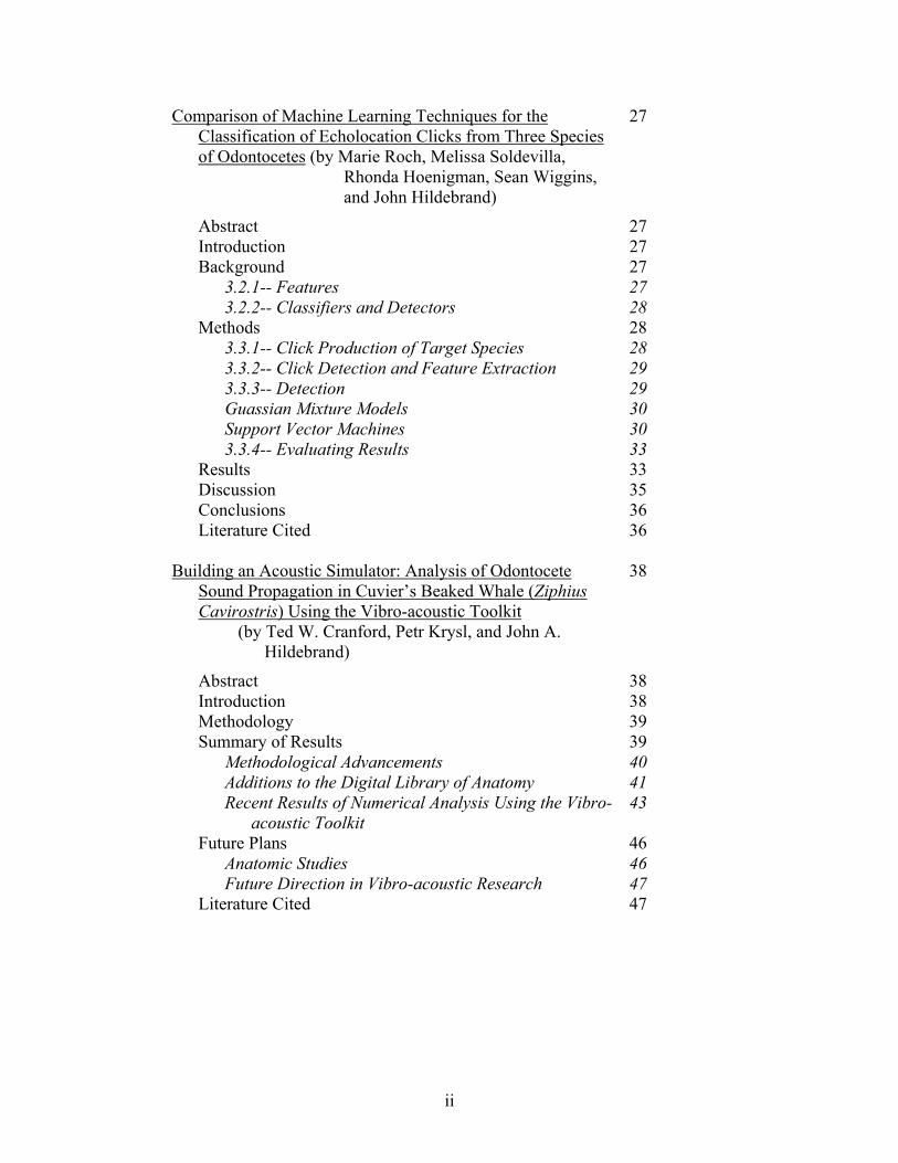
Comparison of Machine Learning Techniques for the Classification of Echolocation Clicks from Three Species of Odontocetes (by Marie Roch, Melissa Soldevilla,

Rhonda Hoenigman, Sean Wiggins, and John Hildebrand)

Abstract Introduction Background

3.2.1-- Features 3.2.2-- Classifiers and Detectors

Methods 3.3.1-- Click Production of Target Species 3.3.2-- Click Detection and Feature Extraction 3.3.3-- Detection Guassian Mixture Models Support Vector Machines 3.3.4-- Evaluating Results

Results Discussion Conclusions Literature Cited

Building an Acoustic Simulator: Analysis of Odontocete

Sound Propagation in Cuvier’s Beaked Whale (Ziphius Cavirostris) Using the Vibro-acoustic Toolkit

(by Ted W. Cranford, Petr Krysl, and John A. Hildebrand)

Abstract Introduction Methodology Summary of Results

Methodological Advancements Additions to the Digital Library of Anatomy Recent Results of Numerical Analysis Using the Vibro-

acoustic Toolkit Future Plans

Anatomic Studies Future Direction in Vibro-acoustic Research

Literature Cited

27

27 27 27 27 28 28 28 29 29 30 30 33 33 35 36 36 38

38 38 39 39 40 41 43 46 46 47 47

iii

PROJECT PUBLICATIONS

Peer-Reviewed Publications Abstracts

INITIAL DISTRIBUTION LIST

49 49 50 52

iv

List of Tables Table 1.1: Table 1.2: Table 2.1: Table 3.1: Table 3.2:

Visual survey information for CalCOFI cruises during our 2007-2008 reporting period. Visual detections of cetaceans over CalCOFI cruises from July 2007-April 2008. Large baleen whale sightings, combined by season, in CalCOFI southern California region (lines 93 through 77), July 2004-March 2008. Equal error rates for jackknifed development data with sixteen mixture GMMs and C 100, 200 for the best parameter set across all jackknife splits. Contents of evaluation files 1-9.

6

8

13

34

34

v

List of Figures Figure 2.1: Figure 2.2: Figure 2.2A: Figure 2.2B: Figure 2.2C: Figure 2.2D: Figure 2.3: Figure 2.4: Figure 3.1: Figure 3.2: Figure 3.3: Figure 3.4:

CalCOFI study area showing numbered ship tracklines, hydrographic and net tow stations, and northern and southern Channel Islands. Whale sightings overlaid on contour maps of SST (left) and zooplankton biomass (right): Legend. Whale sightings overlaid on contour maps of SST (left) and zooplankton biomass (right): Winter cruises 2005-2008. Whale sightings overlaid on contour maps of SST (left) and zooplankton biomass (right): Spring cruises 2005-2008. Whale sightings overlaid on contour maps of SST (left) and zooplankton biomass (right): Summer cruises 2004-2007. Whale sightings overlaid on contour maps of SST (left) and zooplankton biomass (right): Fall cruises 2004-2007. Mean SST for cruise (filled diamonds) and at whale sightings (open squares) for all 16 cruises between July 2004 and April 2008 (cruises 0407-0804), by cruise order (top) and by season (bottom). The natural logarithm of average total zooplankton displacement volumes for cruise (filled diamonds) and at whale sighting locations (open squares) for all 16 cruises between July 2004 and April 2008 (cruises 0407-0804), by cruise order (top) and by season (bottom). Separating hyperplane (solid line) between squares and circles that maximizes the distance between the closest vectors (margin). Squares and circles that are not linearly separable. Hyperplane with dot product kernel (left) vs. Gaussian kernel (right). Detection error tradeoff curves for GMM. Detection error tradeoff curves for SVM.

12

14

15

16

17

18

20

21

31

33

34

34

vi

Figure 4.1: Figure 4.2: Figure 4.3: Figure 4.4: Figure 4.5: Figure 4.6:

Two views from computer reconstructions of five beaked whale specimens that were scanned simultaneously in the same container. Portable reusable immersion tank. Computer reconstructions from CTD scans of Sowerby’s beaked whale (Mesoplodon bidens): right anterolateral view (A), right lateral view (B), and left lateral view (C). Computer reconstructions from segmented CTD scan data of Blainville’s beaked whale, Mesoplodon densirostris. Various views are indicated. Systemic amplification at sensor 1. Systemic amplification at sensor 2.

40

41

42

43

45

46

1

Fleet and Industrial Supply Center

(FISC) N00244-07-1-0011

July 9, 2007 – September 30, 2008 Submitted to:

Naval Postgraduate School

Marine Mammal Acoustic Monitoring and Habitat Investigation,

Southern California Offshore Region

John Hildebrand Marine Physical Laboratory

Scripps Institution of Oceanography

2

Contract Number: N00244-07-1-0011 Project Title: Marine Mammal Acoustic Monitoring and Habitat

Investigation, Southern California Offshore Region Project Duration: July 9, 2007 – September 30, 2008

Executive Summary

This report summarizes work conducted in FY2007-FY2008 with Navy support to conduct marine mammal monitoring and habitat investigations in the southern California offshore region, an area of significant naval training. The report describes results of monitoring for marine mammals during quarterly CalCOFI (California Cooperative Fisheries Investigations) cruises, and models how physical and biological oceanographic conditions affect marine mammal habitat. In addition, we report on progress with constructing automatic detection and classification algorithms for acoustic monitoring of marine mammals. Finally, we report on finite element modeling of acoustic propagation within the bodies of beaked whales and related marine mammals. We investigated the spatial and temporal variation in distributions of three large baleen whale species off southern California in relation to sea surface temperature (SST) and zooplankton displacement volume using Geographic Information System (GIS) software. Data were collected on sixteen CalCOFI quarterly cruises (lines 77-93) from July 2004 - March 2008. The most frequently sighted large whales were humpback whales (67 sightings), fin whales (52 sightings), and blue whales (36 sightings). Blue and humpback whale sightings peaked in summer (July/August) and fin whales were most frequently seen in summer and fall, consistent with known migratory patterns. In spring through fall, sightings were associated with colder SST and greater zooplankton abundance levels compared to averages from random locations on the trackline. These results support the hypothesis that foraging distributions of large whales are linked to cold surface temperatures, which may indicate processes that enhance prey production and accumulation, such as upwelling or advection of productive water within the California Current. However, winter distributions of whales assumed to be migrating do not appear to be related to the habitat variables we analyzed, and may be harder to predict based on oceanographic data. The frequency of CalCOFI cruises provides us with high temporal resolution and long time series compared to other survey efforts, allowing comparison between seasons and years that will increase our understanding of these top predators and their response to habitat variability within an important subregion of the California Current Ecosystem. To assist with analysis of passive acoustic data, we present a species classifier which decides whether or not short groups of clicks are produced by one or more individuals from the following species: Blainville’s beaked whales, short-finned pilot whales, and Risso’s dolphins. The system locates individual clicks using the Teager energy operator and then constructs feature vectors for these clicks using cepstral analysis. Two different types of detectors confirm or reject the presence of each species. Gaussian mixture models (GMMs) are used to model time series independent characteristics of the species feature vector distributions. Support vector machines (SVMs) are used to model the boundaries between each species’ feature distribution and that of other species. Detection error tradeoff curves for all three species are shown with the following equal error rates: Blainville’s beaked whales (GMM 3.32%/SVM 5.54%), pilot whales (GMM 16.18%/SVM 15.00%), and Risso’s dolphins (GMM 0.03%/SVM 0.70%).

3

To understand the propagation of acoustic energy with the bodies of marine mammals, we conducted anatomical investigations and computer finite element modeling. There are five significant research results from our efforts over the past year. Two of these results are methodological advancements. Two other results demonstrate the successful addition of additional beaked whale species (Mesoplodon densirostris and Mesoplodon bidens) to the Digital Library of Anatomy. The primary simulation results are the analysis of propagated acoustic waves incident upon our model of Cuvier’s beaked whale. The primary sound receiving channel (via the gular or throat area) amplifies incident signals. The volume-averaged amplification of up to 5 dB was observed for frequencies between 15 kHz and 35 kHz. Locally the received signal can be boosted significantly higher than the volume averaged pressures would suggest. The locations in the vicinity of the ear bones receiving the highest amplitude signals vary with acoustic frequency. This suggests that different mechanisms (and pathways) may function to transmit sound (pressure) to the cochlea for different frequencies. The simulations of the amplification mechanism of the sound receiving channel do not support conjectures that for the range of sound pressure and frequency parameters considered in the present study the acoustic pressures in the soft tissues surrounding the ears could be boosted to levels that would generate physical damage in tissues. At 5 kHz, the lowest frequency tested, the sound reception anatomy acts as a filter, reducing the received level by 10 to 15 dB below that for the sound incident on the surface of the head.

4

Overview

This report covers scientific research activities conducted by the Scripps Institution of Oceanography during 2007-2008 concerned with understanding cetacean use of sound and their sensitivity to anthropogenic sound. The proposal is a continuation from work conducted in FY2006 with Navy support and addressed four research tasks: (1) passive acoustic monitoring for marine mammals in the SCORE range, (2) modeling how physical and biological oceanographic conditions affect marine mammal habitat, and how habitat features can be used to predict marine mammal distribution and abundance, (3) study of beaked whale acoustic behavior and habitat, and (4) finite element modeling of acoustic propagation within the bodies of beaked whales and related marine mammals. A broad range of mysticetes (baleen whales) and odontocetes (toothed whales) are found in southern California waters and in the Navy’s SCORE range in particular. Mysticetes have been seen off southern California in all seasons, though particular species are more numerous during particular seasons. For instance, Blue (Balaenoptera musculus), fin (Balaenoptera physalus), and humpback (Megaptera novaeangliae) whales are present in greater numbers in the summer and fall as they migrate into the Southern California Bight (Forney and Barlow 1998, Larkman and Veit 1998, Calambokidis and Barlow 2004). Gray whales (Eschrichtius robustus) migrate through the region southbound between November - February and northbound in April - June (Poole 1984). Minke whale (Balaenoptera acutorostrata) and sei whale (Balaenoptera borealis) inhabit southern California waters in all seasons or with unknown seasonal patterns. Some odontocetes are found in southern California offshore waters throughout the year, whereas others migrate into the area on a seasonal basis. Short- and long-beaked common dolphins (Delphinus delphis and Delphinus capensis) (Heyning and Perrin 1994) are typically sighted in schools of hundreds to greater than 1000 individuals. Short-beaked common dolphins are one of the most abundant odontocete species off California, though their abundance varies seasonally and annually as they move offshore and northward in summer months (Forney and Barlow 1998). Conversely, an offshore population of bottlenose dolphins (Tursiops truncatus) occurs during all seasons throughout the Southern California Bight (Forney and Barlow 1998). Risso's dolphins (Grampus griseus), Pacific white-sided dolphins (Lagenorhynchus obliquidens), northern right whale dolphins (Lissodelphis borealis), and Dall’s porpoise (Phocoenoides dalli) exhibit a seasonal presence, moving into waters off California during cold-water months (November – April) and shifting northward to Oregon and Washington or offshore in warmer-water months (May – October) (Green et al. 1992, Forney et al. 1995, Forney and Barlow 1998). Several additional species inhabit southern California waters in all seasons or with unknown seasonal patterns. Among these are the sperm whale (Physeter macrocephalus), killer whale (Orcinus orca), Baird’s beaked whale (Berardius bairdii), pilot whale (Globicephala macrorhynchus), false killer whale (Pseudorca crassidens), Cuvier’s beaked whale (Ziphius cavirostris) and various other beaked whale species (Mesoplodon spp.). Development of acoustic techniques for study of cetaceans is a major focus of this study. Different sounds are made by different species, and documenting these sounds provides a basis for passive acoustic monitoring. The kinds of sounds produced vary by season and by time of day; by making long-term acoustic recordings, we are documenting these temporal variations in sound production. Likewise, since sounds are associated with behaviors, they may reveal the cycle of activities of these animals.

5

By using the R/P FLIP for simultaneous visual and acoustic observations of dolphins, we have discerned differences in vocal behavior. Our study focuses on five delphinid species found in SCORE: Pacific white-sided dolphin, short-beaked common dolphin, long-beaked common dolphin, Risso’s dolphin, and bottlenose dolphin. Behavioral sampling consists of visual observers on R/P FLIP recording focal follows of individual animals or groups of animals, and designating behavior by the following categories: Milling/Resting (variable direction of movement, slow swimming speeds, remain near surface); Foraging (variable direction of movement, high arching dives, fish chasing/tossing); Traveling (move in same direction, steadily/rapidly, often synchronous and frequent surfacing); Social/Surface Active (individuals in close proximity/physical contact, often interacting, frequent surface active behavior). Acoustic behavior (broadband sampling with multiple arrays) allows localization of calling and quantification of whistles, clicks, and burst pulses, as well as other call characteristics, such as inter-click interval, peak frequency, duration, and bandwidth. Thus far 92 groups of delphinids have been analyzed, revealing significantly more echolocation during foraging and less during travel (especially fast travel). Species-distinctive differences have been observed at different times of day and with group size (e.g., large groups of common dolphin tend to travel, whereas small groups tend to mill). These results are important for interpreting long-term acoustic monitoring data. Acoustic call detection and classification by species is a key step in processing acoustic monitoring data. Recent advances in acoustic recording capabilities allow remote autonomous recordings with terabyte data storage (Wiggins and Hildebrand 2007). Manual analyses of these large data sets are prohibitive based on the time and costs for manual analysis. Reliable automated methods are needed for detection and classification of cetacean calls to allow rapid analysis of these large acoustic data sets. Models are needed for how cetaceans are distributed within the ocean environment. These models will allow not only for better understanding of how cetaceans exploit the marine environment, but also the ability to predict the potential for cetaceans to be present at a particular place and time. Our focus has been to collaborate with the CalCOFI to study how marine mammals are distributed with respect to oceanographic parameters such as water temperature and the presence of prey, such as fish and zooplankton.

6

Results

Marine Mammal Observations during 2007-2008 CalCOFI Surveys Lisa Munger, Greg Campbell, Karlina Merkens, Anne Douglas, John Calambokidis and John Hildebrand

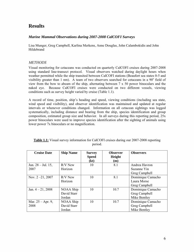
METHODS Visual monitoring for cetaceans was conducted on quarterly CalCOFI cruises during 2007-2008 using standard line-transect protocol. Visual observers watched during daylight hours when weather permitted while the ship transited between CalCOFI stations (Beaufort sea states 0-5 and visibility greater than 1 nm). A team of two observers searched for cetaceans in a 90o field of view from the bow to abeam of the ship, alternating between 7 x 50 power binoculars and the naked eye. Because CalCOFI cruises were conducted on two different vessels, viewing conditions such as survey height varied by cruise (Table 1.1). A record of time, position, ship’s heading and speed, viewing conditions (including sea state, wind speed and visibility), and observer identification was maintained and updated at regular intervals or whenever conditions changed. Information on all cetacean sightings was logged systematically, including distance and bearing from the ship, species identification and group composition, estimated group size and behavior. In all surveys during this reporting period, 25x power binoculars were used to improve species identification after the sighting of animals using lower power 7x binoculars or no magnification.

Table 1.1: Visual survey information for CalCOFI cruises during our 2007-2008 reporting period.

Cruise Date Ship Name Survey

Speed (kt)

Observer Height

(m)

Observers

Jun. 28 – Jul. 15, 2007

R/V New Horizon

10 8.1 Andrea Havron Suzanne Yin Greg Campbell

Nov. 2 –21, 2007 R/V New Horizon

10 8.1 Dominique Camacho Laura Morse Greg Campbell

Jan. 4 – 21, 2008 NOAA Ship David Starr Jordan

10 10.7 Dominique Camacho Greg Campbell Mike Bentley

Mar. 25 – Apr. 9, 2008

NOAA Ship David Starr Jordan

10 10.7 Dominique Camacho Greg Campbell Mike Bentley

7

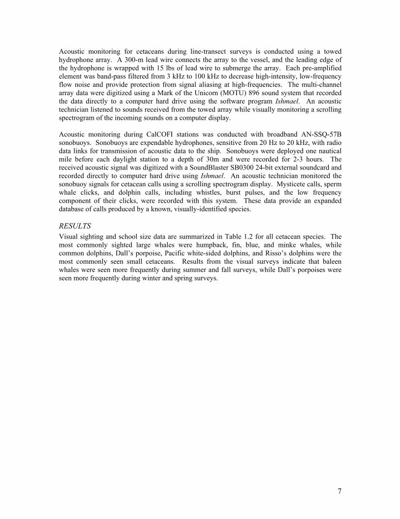
Acoustic monitoring for cetaceans during line-transect surveys is conducted using a towed hydrophone array. A 300-m lead wire connects the array to the vessel, and the leading edge of the hydrophone is wrapped with 15 lbs of lead wire to submerge the array. Each pre-amplified element was band-pass filtered from 3 kHz to 100 kHz to decrease high-intensity, low-frequency flow noise and provide protection from signal aliasing at high-frequencies. The multi-channel array data were digitized using a Mark of the Unicorn (MOTU) 896 sound system that recorded the data directly to a computer hard drive using the software program Ishmael. An acoustic technician listened to sounds received from the towed array while visually monitoring a scrolling spectrogram of the incoming sounds on a computer display. Acoustic monitoring during CalCOFI stations was conducted with broadband AN-SSQ-57B sonobuoys. Sonobuoys are expendable hydrophones, sensitive from 20 Hz to 20 kHz, with radio data links for transmission of acoustic data to the ship. Sonobuoys were deployed one nautical mile before each daylight station to a depth of 30m and were recorded for 2-3 hours. The received acoustic signal was digitized with a SoundBlaster SB0300 24-bit external soundcard and recorded directly to computer hard drive using Ishmael. An acoustic technician monitored the sonobuoy signals for cetacean calls using a scrolling spectrogram display. Mysticete calls, sperm whale clicks, and dolphin calls, including whistles, burst pulses, and the low frequency component of their clicks, were recorded with this system. These data provide an expanded database of calls produced by a known, visually-identified species. RESULTS Visual sighting and school size data are summarized in Table 1.2 for all cetacean species. The most commonly sighted large whales were humpback, fin, blue, and minke whales, while common dolphins, Dall’s porpoise, Pacific white-sided dolphins, and Risso’s dolphins were the most commonly seen small cetaceans. Results from the visual surveys indicate that baleen whales were seen more frequently during summer and fall surveys, while Dall’s porpoises were seen more frequently during winter and spring surveys.

8

Table 1.2: Visual detections of cetaceans over CalCOFI cruises from July 2007 – April 2008. Total number of schools sighted and total number of animals sighted per species for each trip.

July 2007

November 2007

January 2008

April 2008

July 2007 –April 2008

Species #

sight#

animals#

sight#

animals#

sight#

animals#

sight#

animals #

sight #

animals

Blue whale 7 7 1 2 8 9

Fin whale 7 12 1 2 2 6 2 2 12 22

Humpback whale 35 61 1 2 2 4 38 67

Sei whale

Minke whale 3 4 2 2 5 6

Gray whale

Sperm whale 1 2 1 1 2 3

Short-beaked common dolphin 11 529 9 992 4 921 7 514 31 2956

Long-beaked common dolphin 6 794 6 794

Common dolphin species 17 646 8 2293 5 2457 3 857 33 6253

Pacific white-sided dolphin 1 10 2 11 5 59 5 22 13 102

Risso's dolphin 6 87 3 24 2 56 11 167

Northern right-whale dolphin 2 10 2 26 4 36

Bottlenose dolphin 1 25 2 30 3 55

Dall's porpoise 1 4 4 21 14 65 19 90

Short-finned pilot whale 1 33 1 33

Killer whale

Cuvier's beaked whale

Unidentified whale 31 40 21 26 9 10 6 9 67 85

Unidentified dolphin 16 806 5 1720 3 174 24 2700

Unidentified beaked whale

Total 138 3025 56 5093 36 3673 47 1587 277 13378

9

Baleen whale distribution relative to surface temperature and zooplankton abundance off southern California, 2004-2008

Lisa M. Munger, Dominique Camacho, Andrea Havron, Greg Campbell, John Calambokidis, Annie Douglas, and John Hildebrand

Abstract We investigated the spatial and temporal variation in distributions of three large baleen whale species off southern California in relation to sea surface temperature (SST) and zooplankton displacement volume using Geographic Information System (GIS) software. Data were collected on sixteen California Cooperative Oceanic Fisheries Investigations (CalCOFI) quarterly cruises (lines 77-93) from July 2004 - March 2008. The most frequently sighted large whales were humpback whales (67 sightings), fin whales (52 sightings), and blue whales (36 sightings). Blue and humpback whale sightings peaked in summer (July/August) and fin whales were most frequently seen in summer and fall, consistent with known migratory patterns. In spring through fall, sightings were associated with colder SST and greater zooplankton abundance levels compared to averages from random locations on the trackline. These results support the hypothesis that foraging distributions of large whales are linked to cold surface temperatures, which may indicate processes that enhance prey production and accumulation, such as upwelling or advection of productive water within the California Current. However, winter distributions of whales assumed to be migrating do not appear to be related to the habitat variables we analyzed, and may be harder to predict based on oceanographic data. The frequency of CalCOFI cruises provides us with high temporal resolution and long time series compared to other survey efforts, allowing comparison between seasons and years that will increase our understanding of these top predators and their response to habitat variability within an important subregion of the California Current Ecosystem. Introduction Baleen whales are highly mobile apex predators that feed on spatially patchy, ephemeral aggregations of zooplankton. Several baleen whale species seasonally forage and migrate within the productive and dynamic California Current Ecosystem (CCE), which varies markedly on seasonal, interannual and multi-year timescales (Hickey 1979; Hayward and Venrick 1998; Mullin et al. 2000; Brinton and Townsend 2003; Chhak and Di Lorenzo 2007; Keister and Strub 2008). CalCOFI cruises, conducted offshore of southern California every 3 months, provide an excellent platform to observe temporal variation in whale distribution in relation to zooplankton abundance and other habitat variables. The data provided by these frequent surveys and extensive oceanographic measurements may aid in developing predictive models of whale occurrence as a useful management and conservation tool in southern California, a region heavily used by humans for military, industrial, and other activities. Cetacean surveys have been conducted on each CalCOFI cruise since July 2004 using both visual and acoustic detection methods (Soldevilla et al. 2006; Douglas et al. in preparation). The most frequently sighted baleen whales during these and other surveys off southern California are blue (Balaenoptera musculus), fin (Balaenoptera physalus), and humpback (Megaptera novaeangliae) whales, all within the family Balaenopteridae (rorquals) (Smith et al. 1986; Soldevilla et al. 2006; Barlow and Forney 2007). Blue whales off California feed exclusively on euphausiids (‘krill’) (Fiedler et al. 1998), whereas the diets of fin whales and humpback whales include krill as well as copepods, cephalopods, and small schooling fish such as sardines, herring, and anchovies (Fiedler et al. 1998; Flinn et al. 2002; Clapham et al. 1997).

10

Baleen whales forage primarily in summer and typically migrate to lower-latitude breeding and calving grounds in winter, although wintering grounds and movement patterns of fin whales are not well known (Mate et al. 1999, Forney and Barlow 1998, Etnoyer et al. 2006). Whaling records from the early 20th century and recent surveys over the past twenty years indicate that blue and fin whales are most abundant off the coast of California in summer and fall (but also seen occasionally in winter), whereas humpbacks were seen near the coast in summer but further offshore in winter (Clapham et al. 1997; Forney and Barlow 1998). Recent cetacean survey effort off California has been seasonally biased, conducted primarily from ships in summer-fall (Barlow and Forney 2007), except for two winter aerial surveys conducted in 1991 and 1992 (Forney and Barlow 1998). Continuous year-round acoustic monitoring off southern California corroborates that blue whales are present in summer and fall and are rare or absent at other times of year (Burtenshaw et al. 2004; Oleson et al. 2007); fin whale calls, although most abundant in summer through fall, are detected year-round (Oleson 2005). The foraging distributions of baleen whales off California vary depending on where and when their prey, especially euphausiids (for blue and fin whales), are concentrated, which is determined by marine ecosystem features and dynamic climactic and oceanic processes. Circulation within the southern California Bight is characterized by the cold, equatorward-flowing California Current (CC) centered about 200-300 km offshore, and the strengthening in summer to fall of the southern California Eddy and southern California countercurrent, which brings warm water northward along the coast (Hickey 1992). In the CCE, wind-driven coastal upwelling in spring promotes high primary productivity (as indicated by chlorophyll concentration), with a subsequent increase in zooplankton production that reaches a peak in adult biomass after a time lag of 1-4 months (Hayward and Venrick 1998). This time lag corresponds to the interval between peak surface chlorophyll concentration and peak whale abundance off California (Burtenshaw et al. 2004; Croll et al. 2005). As upwelled, productive waters are advected southward by the CC, dense euphausiid patches may develop in areas where bottom topography and/or other features (such as eddies and fronts) contribute to retention, such as in Monterey Bay (Croll et al. 2005) and around the Channel Islands (Fiedler et al. 1998). Keiper et al. (2005) recorded greater marine mammal sighting rates during periods of upwelling relaxation/stronger stratification in early to late spring surveys, and hypothesized that these conditions contribute to stabilization and aggregation of prey. Climatic oscillations on annual and multiyear timescales contribute to variability in production within the CCE and hence distribution of whales. For example, cetacean surveys in Monterey Bay during the late 1990s documented decreased balaenopterid whale abundance during the 1997 onset of El Nino, when krill acoustic backscatter was low, and then a sharp increase in whales as krill abundance slowly increased in 1998 (Benson et al. 2002). The authors hypothesized that the sharp increase in whale numbers within the bay was due to whales concentrating in inshore productive areas while offshore krill abundance remained low through the El Nino event. Over the past couple of decades, large-scale population assessment surveys conducted by the U.S. National Marine Fisheries Service (NMFS) provide evidence for blue whales shifting foraging grounds outside of the California-Oregon-Washington study area (Barlow and Forney 2007; Barlow et al. 2008a). This shift in blue whale distribution may be associated with the overall declining trend in zooplankton displacement volumes off California since the 1990s (Goericke et al. 2007; McClatchie et al. 2008). However, NMFS surveys are conducted every 3-5 years primarily in summer and fall, and as such do not capture seasonal variability between years. The CalCOFI program has conducted four cruises per year since 1949 that presently measure over 20 meteorological, oceanographic and biological variables. Since 2004, CalCOFI cruises have included systematic marine mammal visual and acoustic surveys, providing an opportunity

11

to investigate the relationship of top marine predators to these numerous habitat variables. Previous studies in the CCE have found that baleen whale distributions are related to season and environmental variables, including bathymetry, sea surface temperature, salinity, location of fronts, chlorophyll concentration, and acoustic backscatter (Smith et al. 1986; Burtenshaw et al. 2004; Keiper et al. 2005; Tynan et al. 2005; Etnoyer et al. 2006). However, habitat models are often limited by small sample sizes due to infrequent surveys/low numbers of sightings, lack of data during winter months when surveys are not typically conducted, and/or by availability of oceanographic data. For example, many studies incorporate bathymetry and remotely-sensed ocean surface data from satellites because these data are widely available, but assumptions are required to explain physical and biological mechanisms by which surface production is transferred to macrozooplankton in dense aggregations needed to support apex predators. This paper provides a preliminary descriptive overview of spatiotemporal patterns in selected habitat variables and cetacean distributions within the southern California Bight. We examined two habitat variables measured in situ during CalCOFI cruises, sea surface temperature (SST) and zooplankton displacement volume, in relation to concurrent whale sightings data. We selected sea surface temperature due to its potential to indicate physical mechanisms that lead to either production (e.g., upwelling or advection of cold, nutrient-rich water) or concentration (e.g., along temperature fronts or eddies) of prey. Zooplankton displacement volume, a proxy for abundance, does not directly measure krill abundance. However, where there are small zooplankton, there will also be larger zooplankton as well as other prey, such as fish. This suggests that zooplankton displacement volume may indirectly represent whale forage conditions. Identifying potential patterns and linkages between whale distributions, prey, and oceanographic variables will allow the formulation of hypotheses that can be tested using more rigorous statistical methods. Materials and Methods

Data collection

Data were collected during CalCOFI cruises off southern California (Figure 2.1) from July 2004 through March 2008 using Scripps Institution of Oceanography (SIO) research vessels New Horizon (NH), Roger Revelle (RR) and the National Oceanic and Atmospheric Administration (NOAA) research vessel David Starr Jordan (JD). Two trained marine mammal observers were posted on the bridge wings (NH, 8.1m above water), flying bridge (JD, 11m), or 03 level (RR, 13.2m), and equipped with 7 x 50 power binoculars to locate and identify cetaceans as the ship transited between stations at 10 knots. Ship time constraints did not allow deviation from the trackline to approach unidentified cetaceans; however, “big eye” binoculars (25 x 50 power) were available in November 2004 and during all cruises since July 2005 (JD and RR = constant access, NH = restricted access) to aid in species identification at long distances (Soldevilla et al. 2006). Mammal observers recorded sighting information including species, group size (estimated by consensus), behavior, weather and sea state. The latter two variables were also recorded periodically independent of sightings. Survey effort was curtailed in sea states of Beaufort 6 or greater, or when visibility was reduced to less than 1 km. Mammal observers recorded opportunistic sightings during non-standard transits, poor visibility, and/or while on station; but these were not used in this analysis.

12

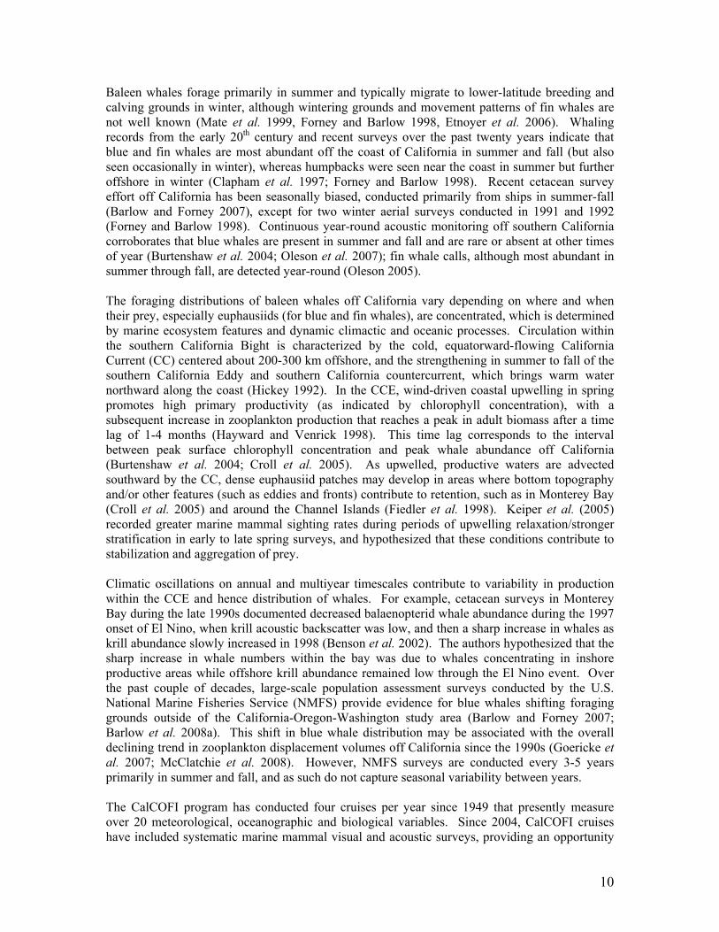
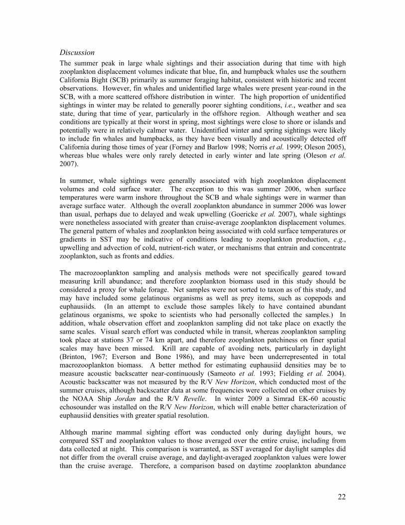
Figure 2.1: CalCOFI study area showing numbered ship tracklines, hydrographic and net tow stations, and northern and southern Channel Islands. 2000 m depth contour is shown in grey.

Sea surface temperature (SST) and other ocean surface data were collected at approximately 2 m depth using the ship hull-mounted system and Seabird Electronics SBE-21 thermosalinograph or similar. Underway data were collected at 30-second intervals and processed with 10-minute time resolution. Underway data from the NOAA Ship David Starr Jordan were not available during 2007 and 2008 winter cruises (CC0701 and CC0801). For these cruises we analyzed on-station temperature data from CTD sensors and bottles. Zooplankton were sampled at CalCOFI stations with a standard oblique plankton tow to 210 meters (bottom depth permitting) using Bongo paired 505 m mesh nets with 71 cm diameter openings. Total zooplankton volumes (ml) were standardized to water volume (per 1000 cubic meter strained volume). For this analysis, we removed high outlier zooplankton displacement volumes (likely due to overabundance of gelatinous species) (A. Hays, personal communication).

Data analysis

We used Geographic Information Systems (GIS) software to analyze whale sightings in relation to oceanographic data. Zooplankton displacement volumes, SST, and sightings of

13

blue, fin, humpback, and unidentified balaenopterid whales were uploaded into ArcGIS 9.2 and analyzed using Geostatistical Analyst. Zooplankton volume and SST coverages were created using two interpolation methodologies. A universal Kriging analysis was applied to the 10-minute averaged underway SST data, accounting for a northwest directional second-degree polynomial trend in temperature (Royle et al. 1981; Oliver and Webster 1990; ESRI 2008). Because of smaller sample size and greater spacing between data points, an Inverse Distance Weighted (IDW) analysis (Watson and Philip 1985; ESRI 2008) was applied to data collected at CalCOFI stations. Station data analyzed using IDW included zooplankton displacement volumes and CTD bottle temperature data for cruises 0701, 0801, and 0804 (January 2007, January 2008, and April 2008, respectively). To ensure that the different interpolations produced similar contour maps for underway data and station data, we resampled underway data for four cruises (one each season) at intervals mimicking station spacing, and compared the IDW product to the Kriging product for full-resolution data. Whale sighting locations recorded during on-effort observer transits were overlaid onto zooplankton displacement volume and SST coverages to produce contour maps for each cruise. Line segments representing visual search effort were constructed and depicted on contour maps. Zooplankton displacement volume and SST were extracted at each sighting location. We compared the average seasonal zooplankton and SST values extrapolated at whale sightings to averages for the same number of random locations along on-effort tracklines.

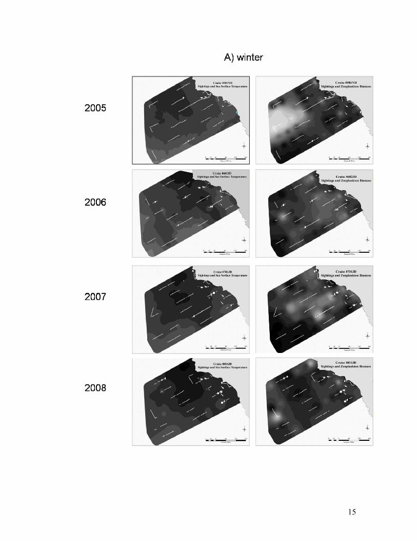
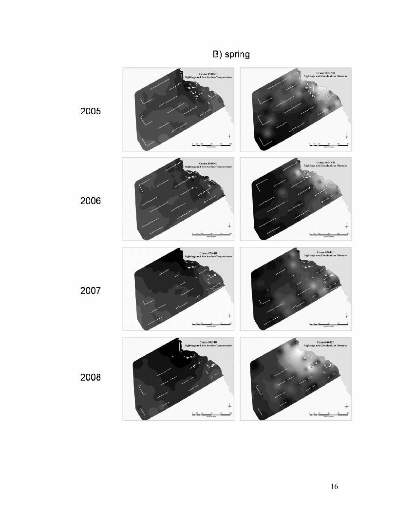
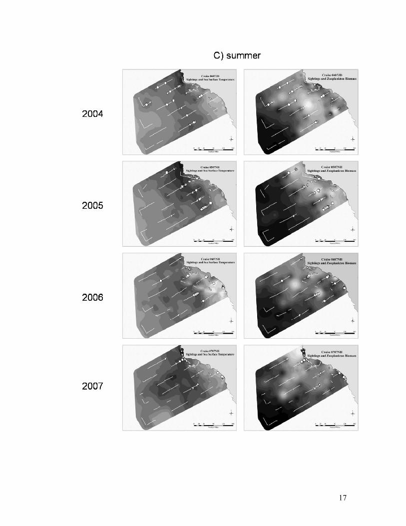
Results The sighting rates of blue, fin, and humpback whales varied seasonally and spatially. Total large baleen whale sightings, including unidentified sightings, were greatest in summer and fall (Table 2.1). Blue and humpback whale sightings were most abundant during summer cruises (July-August); fin whales were seen with almost equal frequency in summer and fall (October-November). Blue whales were not seen in winter (January-February) or spring (March-April), whereas fin whales were observed year-round and humpback whales were frequently seen in spring and fall. Unidentified large whale sightings accounted for about 40% of the total sightings in spring and summer, 54% in fall, and over 90% in winter. Humpback whale sightings were predominantly on the shelf (< 2000 m depth; see Figure 2.1), concentrated near Point Conception and the Channel Islands, whereas blue and fin whale distributions extended further offshore (Figure 2.2). Douglas et al. (in preparation) provide a more detailed analysis of cetacean seasonality and inshore/offshore patterns observed during CalCOFI cruises.

Table 2.1: Large baleen whale sightings, combined by season, in CalCOFI southern California region (lines 93 through 77), July 2004 – March 2008

Winter Spring Summer Fall TOTAL

Blue Whale 0 0 31 5 36 Fin Whale 3 4 23 22 52 Humpback Whale 0 13 36 18 67 Unidentified Baleen Whale 22 10 54 51 137

TOTAL 25 27 144 96 292

14

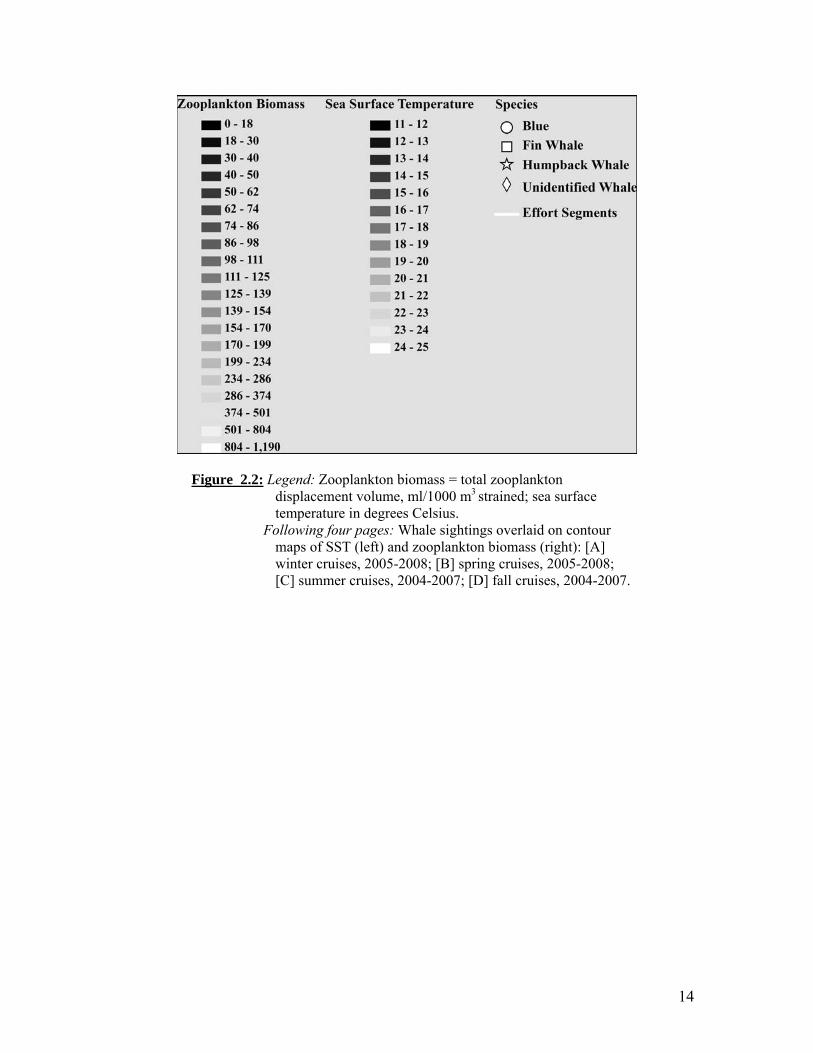
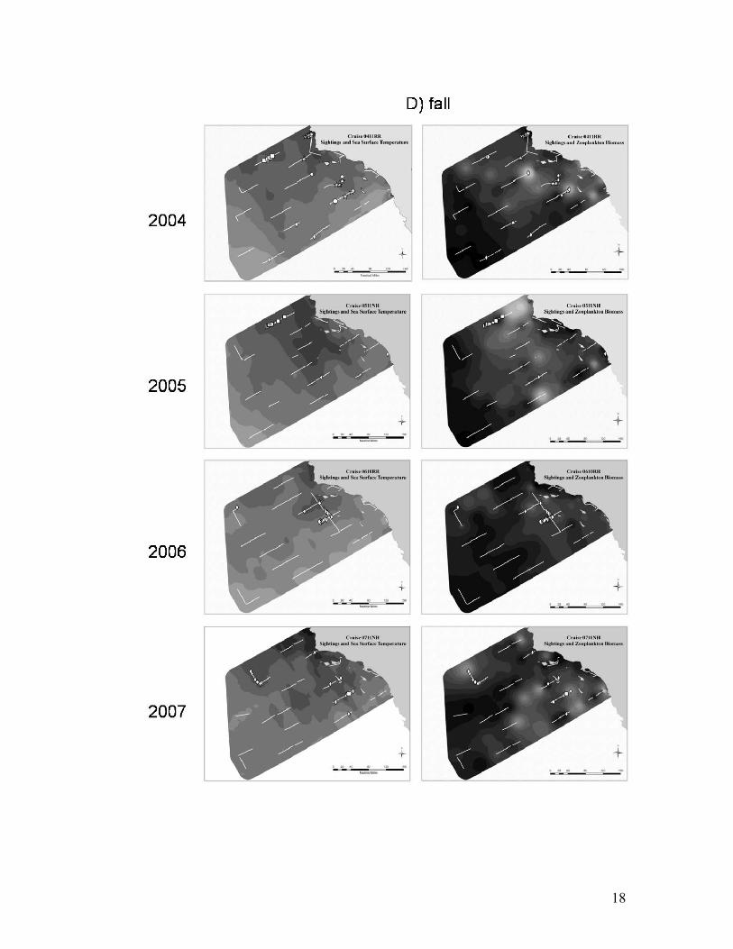
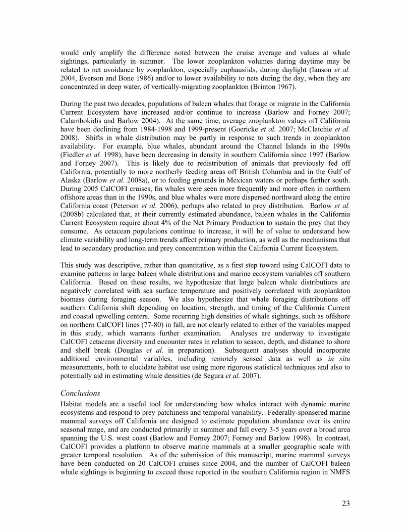
Figure 2.2: Legend: Zooplankton biomass = total zooplankton displacement volume, ml/1000 m3 strained; sea surface temperature in degrees Celsius.

Following four pages: Whale sightings overlaid on contour maps of SST (left) and zooplankton biomass (right): [A] winter cruises, 2005-2008; [B] spring cruises, 2005-2008; [C] summer cruises, 2004-2007; [D] fall cruises, 2004-2007.

15

16

17

18

19

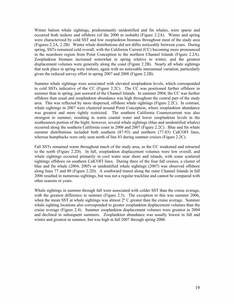
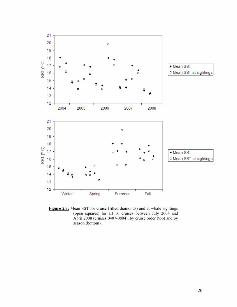
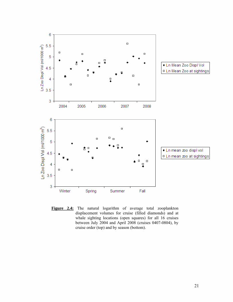
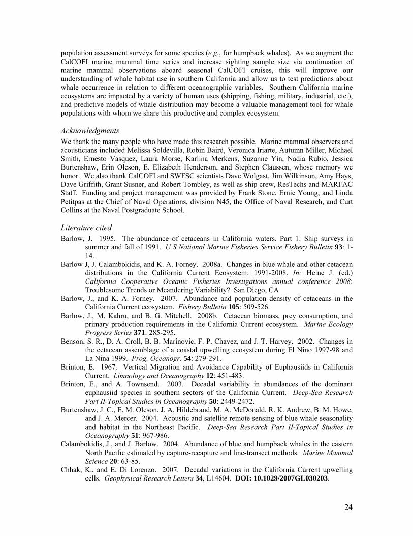
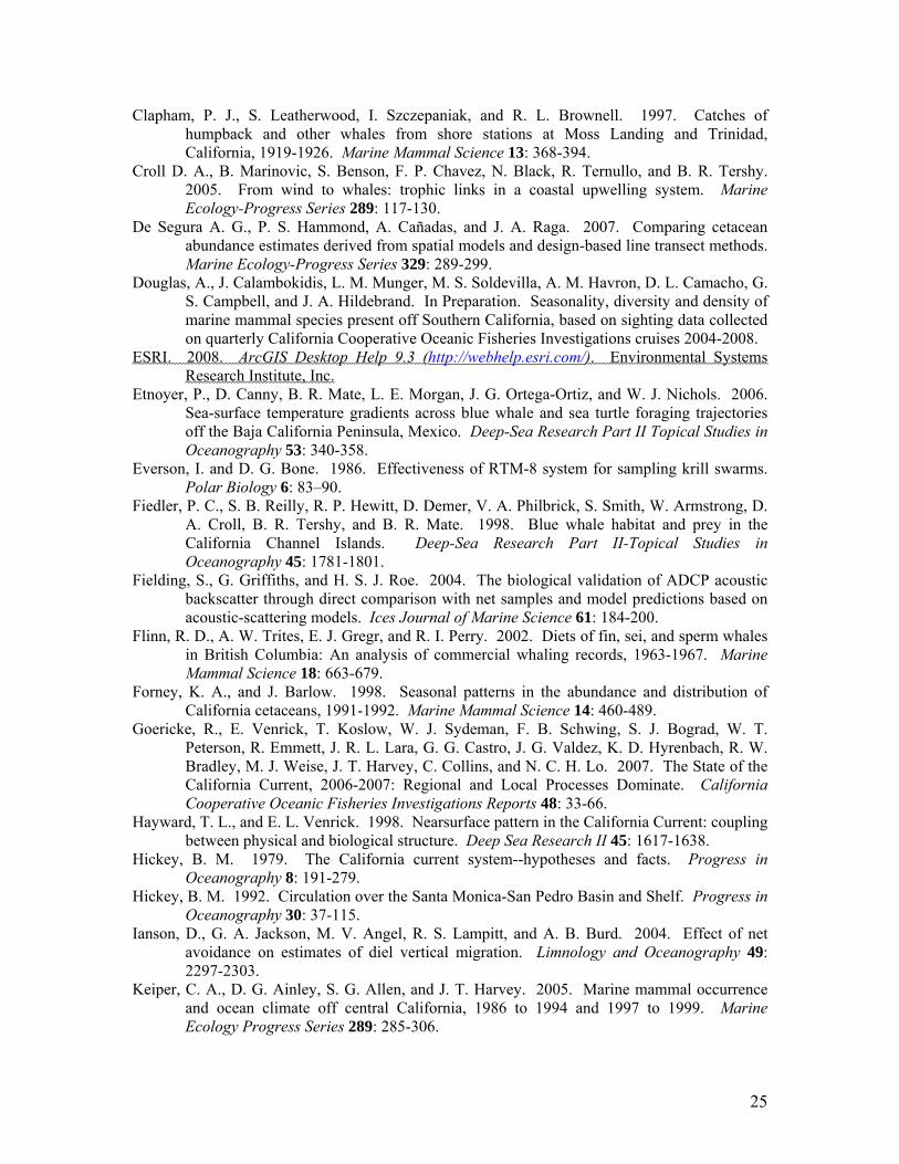
Winter baleen whale sightings, predominantly unidentified and fin whales, were sparse and occurred both inshore and offshore (of the 2000 m isobath) (Figure 2.2A). Winter and spring were characterized by cold SST and low zooplankton biomass throughout most of the study area (Figures 2.2A, 2.2B). Winter whale distributions did not differ noticeably between years. During spring, SSTs remained cold overall, with the California Current (CC) becoming more pronounced in the nearshore region from Point Conception to the northern Channel Islands (Figure 2.2A). Zooplankton biomass increased somewhat in spring relative to winter, and the greatest displacement volumes were generally along the coast (Figure 2.2B). Nearly all whale sightings that took place in spring were inshore, again with no noticeable interannual variation, particularly given the reduced survey effort in spring 2007 and 2008 (Figure 2.2B). Summer whale sightings were associated with elevated zooplankton levels, which corresponded to cold SSTs indicative of the CC (Figure 2.2C). The CC was positioned further offshore in summer than in spring, just seaward of the Channel Islands. In summer 2004, the CC was further offshore than usual and zooplankton abundance was high throughout the central part of the study area. This was reflected by more dispersed, offshore whale sightings (Figure 2.2C). In contrast, whale sightings in 2007 were clustered around Point Conception, where zooplankton abundance was greatest and more tightly restricted. The southern California Countercurrent was also strongest in summer, resulting in warm coastal water and lower zooplankton levels in the southeastern portion of the bight; however, several whale sightings (blue and unidentified whales) occurred along the southern California coast in 2006 and 2007 (Figure 2.2C). Blue and fin whale summer distributions included both southern (87-93) and northern (77-83) CalCOFI lines, whereas humpbacks were only seen north of line 83 during summer cruises (Figure 2.2C). Fall SSTs remained warm throughout much of the study area, as the CC weakened and retracted to the north (Figure 2.2D). In fall, zooplankton displacement volumes were low overall, and whale sightings occurred primarily in cool water near shore and islands, with some scattered sightings offshore on southern CalCOFI lines. During three of the four fall cruises, a cluster of blue and fin whale (2004, 2005) or unidentified whale sightings (2007) was observed offshore along lines 77 and 80 (Figure 2.2D). A southward transit along the outer Channel Islands in fall 2006 resulted in numerous sightings, but was not a regular trackline and cannot be compared with other seasons or years. Whale sightings in summer through fall were associated with colder SST than the cruise average, with the greatest difference in summer (Figure 2.3). The exception to this was summer 2006, when the mean SST at whale sightings was almost 2º C greater than the cruise average. Summer whale sighting locations also corresponded to greater zooplankton displacement volumes than the cruise average (Figure 2.4). Summer zooplankton displacement volumes were greatest in 2004 and declined in subsequent summers. Zooplankton abundance was usually lowest in fall and winter and greatest in summer, but was high in fall 2007 through spring 2008.

20

Figure 2.3: Mean SST for cruise (filled diamonds) and at whale sightings (open squares) for all 16 cruises between July 2004 and April 2008 (cruises 0407-0804), by cruise order (top) and by season (bottom).

21

Figure 2.4: The natural logarithm of average total zooplankton

displacement volumes for cruise (filled diamonds) and at whale sighting locations (open squares) for all 16 cruises between July 2004 and April 2008 (cruises 0407-0804), by cruise order (top) and by season (bottom).

22

Discussion The summer peak in large whale sightings and their association during that time with high zooplankton displacement volumes indicate that blue, fin, and humpback whales use the southern California Bight (SCB) primarily as summer foraging habitat, consistent with historic and recent observations. However, fin whales and unidentified large whales were present year-round in the SCB, with a more scattered offshore distribution in winter. The high proportion of unidentified sightings in winter may be related to generally poorer sighting conditions, i.e., weather and sea state, during that time of year, particularly in the offshore region. Although weather and sea conditions are typically at their worst in spring, most sightings were close to shore or islands and potentially were in relatively calmer water. Unidentified winter and spring sightings were likely to include fin whales and humpbacks, as they have been visually and acoustically detected off California during those times of year (Forney and Barlow 1998; Norris et al. 1999; Oleson 2005), whereas blue whales were only rarely detected in early winter and late spring (Oleson et al. 2007). In summer, whale sightings were generally associated with high zooplankton displacement volumes and cold surface water. The exception to this was summer 2006, when surface temperatures were warm inshore throughout the SCB and whale sightings were in warmer than average surface water. Although the overall zooplankton abundance in summer 2006 was lower than usual, perhaps due to delayed and weak upwelling (Goericke et al. 2007), whale sightings were nonetheless associated with greater than cruise-average zooplankton displacement volumes. The general pattern of whales and zooplankton being associated with cold surface temperatures or gradients in SST may be indicative of conditions leading to zooplankton production, e.g., upwelling and advection of cold, nutrient-rich water, or mechanisms that entrain and concentrate zooplankton, such as fronts and eddies. The macrozooplankton sampling and analysis methods were not specifically geared toward measuring krill abundance; and therefore zooplankton biomass used in this study should be considered a proxy for whale forage. Net samples were not sorted to taxon as of this study, and may have included some gelatinous organisms as well as prey items, such as copepods and euphausiids. (In an attempt to exclude those samples likely to have contained abundant gelatinous organisms, we spoke to scientists who had personally collected the samples.) In addition, whale observation effort and zooplankton sampling did not take place on exactly the same scales. Visual search effort was conducted while in transit, whereas zooplankton sampling took place at stations 37 or 74 km apart, and therefore zooplankton patchiness on finer spatial scales may have been missed. Krill are capable of avoiding nets, particularly in daylight (Brinton, 1967; Everson and Bone 1986), and may have been underrepresented in total macrozooplankton biomass. A better method for estimating euphausiid densities may be to measure acoustic backscatter near-continuously (Sameoto et al. 1993; Fielding et al. 2004). Acoustic backscatter was not measured by the R/V New Horizon, which conducted most of the summer cruises, although backscatter data at some frequencies were collected on other cruises by the NOAA Ship Jordan and the R/V Revelle. In winter 2009 a Simrad EK-60 acoustic echosounder was installed on the R/V New Horizon, which will enable better characterization of euphausiid densities with greater spatial resolution. Although marine mammal sighting effort was conducted only during daylight hours, we compared SST and zooplankton values to those averaged over the entire cruise, including from data collected at night. This comparison is warranted, as SST averaged for daylight samples did not differ from the overall cruise average, and daylight-averaged zooplankton values were lower than the cruise average. Therefore, a comparison based on daytime zooplankton abundance

23

would only amplify the difference noted between the cruise average and values at whale sightings, particularly in summer. The lower zooplankton volumes during daytime may be related to net avoidance by zooplankton, especially euphausiids, during daylight (Ianson et al. 2004, Everson and Bone 1986) and/or to lower availability to nets during the day, when they are concentrated in deep water, of vertically-migrating zooplankton (Brinton 1967). During the past two decades, populations of baleen whales that forage or migrate in the California Current Ecosystem have increased and/or continue to increase (Barlow and Forney 2007; Calambokidis and Barlow 2004). At the same time, average zooplankton values off California have been declining from 1984-1998 and 1999-present (Goericke et al. 2007; McClatchie et al. 2008). Shifts in whale distribution may be partly in response to such trends in zooplankton availability. For example, blue whales, abundant around the Channel Islands in the 1990s (Fiedler et al. 1998), have been decreasing in density in southern California since 1997 (Barlow and Forney 2007). This is likely due to redistribution of animals that previously fed off California, potentially to more northerly feeding areas off British Columbia and in the Gulf of Alaska (Barlow et al. 2008a), or to feeding grounds in Mexican waters or perhaps further south. During 2005 CalCOFI cruises, fin whales were seen more frequently and more often in northern offshore areas than in the 1990s, and blue whales were more dispersed northward along the entire California coast (Peterson et al. 2006), perhaps also related to prey distribution. Barlow et al. (2008b) calculated that, at their currently estimated abundance, baleen whales in the California Current Ecosystem require about 4% of the Net Primary Production to sustain the prey that they consume. As cetacean populations continue to increase, it will be of value to understand how climate variability and long-term trends affect primary production, as well as the mechanisms that lead to secondary production and prey concentration within the California Current Ecosystem. This study was descriptive, rather than quantitative, as a first step toward using CalCOFI data to examine patterns in large baleen whale distributions and marine ecosystem variables off southern California. Based on these results, we hypothesize that large baleen whale distributions are negatively correlated with sea surface temperature and positively correlated with zooplankton biomass during foraging season. We also hypothesize that whale foraging distributions off southern California shift depending on location, strength, and timing of the California Current and coastal upwelling centers. Some recurring high densities of whale sightings, such as offshore on northern CalCOFI lines (77-80) in fall, are not clearly related to either of the variables mapped in this study, which warrants further examination. Analyses are underway to investigate CalCOFI cetacean diversity and encounter rates in relation to season, depth, and distance to shore and shelf break (Douglas et al. in preparation). Subsequent analyses should incorporate additional environmental variables, including remotely sensed data as well as in situ measurements, both to elucidate habitat use using more rigorous statistical techniques and also to potentially aid in estimating whale densities (de Segura et al. 2007). Conclusions Habitat models are a useful tool for understanding how whales interact with dynamic marine ecosystems and respond to prey patchiness and temporal variability. Federally-sponsered marine mammal surveys off California are designed to estimate population abundance over its entire seasonal range, and are conducted primarily in summer and fall every 3-5 years over a broad area spanning the U.S. west coast (Barlow and Forney 2007; Forney and Barlow 1998). In contrast, CalCOFI provides a platform to observe marine mammals at a smaller geographic scale with greater temporal resolution. As of the submission of this manuscript, marine mammal surveys have been conducted on 20 CalCOFI cruises since 2004, and the number of CalCOFI baleen whale sightings is beginning to exceed those reported in the southern California region in NMFS

24

population assessment surveys for some species (e.g., for humpback whales). As we augment the CalCOFI marine mammal time series and increase sighting sample size via continuation of marine mammal observations aboard seasonal CalCOFI cruises, this will improve our understanding of whale habitat use in southern California and allow us to test predictions about whale occurrence in relation to different oceanographic variables. Southern California marine ecosystems are impacted by a variety of human uses (shipping, fishing, military, industrial, etc.), and predictive models of whale distribution may become a valuable management tool for whale populations with whom we share this productive and complex ecosystem. Acknowledgments We thank the many people who have made this research possible. Marine mammal observers and acousticians included Melissa Soldevilla, Robin Baird, Veronica Iriarte, Autumn Miller, Michael Smith, Ernesto Vasquez, Laura Morse, Karlina Merkens, Suzanne Yin, Nadia Rubio, Jessica Burtenshaw, Erin Oleson, E. Elizabeth Henderson, and Stephen Claussen, whose memory we honor. We also thank CalCOFI and SWFSC scientists Dave Wolgast, Jim Wilkinson, Amy Hays, Dave Griffith, Grant Susner, and Robert Tombley, as well as ship crew, ResTechs and MARFAC Staff. Funding and project management was provided by Frank Stone, Ernie Young, and Linda Petitpas at the Chief of Naval Operations, division N45, the Office of Naval Research, and Curt Collins at the Naval Postgraduate School. Literature cited Barlow, J. 1995. The abundance of cetaceans in California waters. Part 1: Ship surveys in

summer and fall of 1991. U S National Marine Fisheries Service Fishery Bulletin 93: 1-14.

Barlow J, J. Calambokidis, and K. A. Forney. 2008a. Changes in blue whale and other cetacean distributions in the California Current Ecosystem: 1991-2008. In: Heine J. (ed.) California Cooperative Oceanic Fisheries Investigations annual conference 2008: Troublesome Trends or Meandering Variability? San Diego, CA

Barlow, J., and K. A. Forney. 2007. Abundance and population density of cetaceans in the California Current ecosystem. Fishery Bulletin 105: 509-526.

Barlow, J., M. Kahru, and B. G. Mitchell. 2008b. Cetacean biomass, prey consumption, and primary production requirements in the California Current ecosystem. Marine Ecology Progress Series 371: 285-295.

Benson, S. R., D. A. Croll, B. B. Marinovic, F. P. Chavez, and J. T. Harvey. 2002. Changes in the cetacean assemblage of a coastal upwelling ecosystem during El Nino 1997-98 and La Nina 1999. Prog. Oceanogr. 54: 279-291.

Brinton, E. 1967. Vertical Migration and Avoidance Capability of Euphausiids in California Current. Limnology and Oceanography 12: 451-483.

Brinton, E., and A. Townsend. 2003. Decadal variability in abundances of the dominant euphausiid species in southern sectors of the California Current. Deep-Sea Research Part II-Topical Studies in Oceanography 50: 2449-2472.

Burtenshaw, J. C., E. M. Oleson, J. A. Hildebrand, M. A. McDonald, R. K. Andrew, B. M. Howe, and J. A. Mercer. 2004. Acoustic and satellite remote sensing of blue whale seasonality and habitat in the Northeast Pacific. Deep-Sea Research Part II-Topical Studies in Oceanography 51: 967-986.

Calambokidis, J., and J. Barlow. 2004. Abundance of blue and humpback whales in the eastern North Pacific estimated by capture-recapture and line-transect methods. Marine Mammal Science 20: 63-85.

Chhak, K., and E. Di Lorenzo. 2007. Decadal variations in the California Current upwelling cells. Geophysical Research Letters 34, L14604. DOI: 10.1029/2007GL030203.

25

Clapham, P. J., S. Leatherwood, I. Szczepaniak, and R. L. Brownell. 1997. Catches of humpback and other whales from shore stations at Moss Landing and Trinidad, California, 1919-1926. Marine Mammal Science 13: 368-394.

Croll D. A., B. Marinovic, S. Benson, F. P. Chavez, N. Black, R. Ternullo, and B. R. Tershy. 2005. From wind to whales: trophic links in a coastal upwelling system. Marine Ecology-Progress Series 289: 117-130.

De Segura A. G., P. S. Hammond, A. Cañadas, and J. A. Raga. 2007. Comparing cetacean abundance estimates derived from spatial models and design-based line transect methods. Marine Ecology-Progress Series 329: 289-299.

Douglas, A., J. Calambokidis, L. M. Munger, M. S. Soldevilla, A. M. Havron, D. L. Camacho, G. S. Campbell, and J. A. Hildebrand. In Preparation. Seasonality, diversity and density of marine mammal species present off Southern California, based on sighting data collected on quarterly California Cooperative Oceanic Fisheries Investigations cruises 2004-2008.

ESRI. 2008. ArcGIS Desktop Help 9.3 (http://webhelp.esri.com/). Environmental Systems Research Institute, Inc.

Etnoyer, P., D. Canny, B. R. Mate, L. E. Morgan, J. G. Ortega-Ortiz, and W. J. Nichols. 2006. Sea-surface temperature gradients across blue whale and sea turtle foraging trajectories off the Baja California Peninsula, Mexico. Deep-Sea Research Part II Topical Studies in Oceanography 53: 340-358.

Everson, I. and D. G. Bone. 1986. Effectiveness of RTM-8 system for sampling krill swarms. Polar Biology 6: 83–90.

Fiedler, P. C., S. B. Reilly, R. P. Hewitt, D. Demer, V. A. Philbrick, S. Smith, W. Armstrong, D. A. Croll, B. R. Tershy, and B. R. Mate. 1998. Blue whale habitat and prey in the California Channel Islands. Deep-Sea Research Part II-Topical Studies in Oceanography 45: 1781-1801.

Fielding, S., G. Griffiths, and H. S. J. Roe. 2004. The biological validation of ADCP acoustic backscatter through direct comparison with net samples and model predictions based on acoustic-scattering models. Ices Journal of Marine Science 61: 184-200.

Flinn, R. D., A. W. Trites, E. J. Gregr, and R. I. Perry. 2002. Diets of fin, sei, and sperm whales in British Columbia: An analysis of commercial whaling records, 1963-1967. Marine Mammal Science 18: 663-679.

Forney, K. A., and J. Barlow. 1998. Seasonal patterns in the abundance and distribution of California cetaceans, 1991-1992. Marine Mammal Science 14: 460-489.

Goericke, R., E. Venrick, T. Koslow, W. J. Sydeman, F. B. Schwing, S. J. Bograd, W. T. Peterson, R. Emmett, J. R. L. Lara, G. G. Castro, J. G. Valdez, K. D. Hyrenbach, R. W. Bradley, M. J. Weise, J. T. Harvey, C. Collins, and N. C. H. Lo. 2007. The State of the California Current, 2006-2007: Regional and Local Processes Dominate. California Cooperative Oceanic Fisheries Investigations Reports 48: 33-66.

Hayward, T. L., and E. L. Venrick. 1998. Nearsurface pattern in the California Current: coupling between physical and biological structure. Deep Sea Research II 45: 1617-1638.

Hickey, B. M. 1979. The California current system--hypotheses and facts. Progress in Oceanography 8: 191-279.

Hickey, B. M. 1992. Circulation over the Santa Monica-San Pedro Basin and Shelf. Progress in Oceanography 30: 37-115.

Ianson, D., G. A. Jackson, M. V. Angel, R. S. Lampitt, and A. B. Burd. 2004. Effect of net avoidance on estimates of diel vertical migration. Limnology and Oceanography 49: 2297-2303.

Keiper, C. A., D. G. Ainley, S. G. Allen, and J. T. Harvey. 2005. Marine mammal occurrence and ocean climate off central California, 1986 to 1994 and 1997 to 1999. Marine Ecology Progress Series 289: 285-306.

26

Keister, J. E., and P. T. Strub. 2008. Spatial and interannual variability in mesoscale circulation in the northern California Current System. Journal of Geophysical Research-Oceans 113, C04015. DOI: 10.1029/2007JC004256.

Mate, B. R., B. A. Lagerquist, and J. Calambokidis. 1999, Movements of North Pacific blue whales during the feeding season off Southern California and their southern fall migration. Marine Mammal Science 15: 1246-1257.

McClatchie, S., R. Goericke, J. A. Koslow, F. B. Schwing, S. J. Bograd, R. Charter, W. Watson, N. Lo, K. Hill, J. Gottschalk, M. L’Heureux, Y. Xue, W. T. Peterson, R. Emmett, C. Collins, G. Gaxiola-Castro, R. Durazo, M. Kahru, B. G. Mitchell, K. D. Hyrenbach, W. J. Sydeman, R. W. Bradley, P. Warzybok, and E. Bjorkstedt. 2008. The State of the California Current, 2007–2008: La Niña Conditions and Their Effects on the Ecosystem. California Cooperative Oceanic Fisheries Investigations Reports 49: 39-76.

Mullin, M. M., E. Goetze, S. E. Beaulieu, and J. M. Lasker. 2000. Comparisons within and between years resulting in contrasting recruitment of Pacific hake (Merluccius productus) in the California Current System. Canadian Journal of Fisheries and Aquatic Sciences 57: 1434-1447.

Norris, T. F., M. McDonald, and J. Barlow. 1999. Acoustic detections of singing humpback whales (Megaptera novaeangliae) in the eastern North Pacific during their northbound migration. Journal of the Acoustical Society of America 106: 506-514.

Oleson, E. M. 2005. Calling behavior of blue and fin whales off California. Ph.D., University of California, San Diego.

Oleson, E. M., S. M. Wiggins, and J. A. Hildebrand. 2007. Temporal separation of blue whale call types on a southern California feeding ground. Animal Behaviour 74: 881-894.

Oliver, M. A., and R. Webster. 1990. Kriging: a method of interpolation for geographical information systems. International Journal of Geographical Information Science 4: 313–332.

Peterson, W. T., R. Emmett, R. Goericke, E. Venrick, A. Mantyla, S. J. Bograd, F. B. Schwing, R. Hewitt, N. Lo, W. Watson, J. Barlow, M. Lowry, S. Ralston, K. A. Forney, B. E. Lavaniegos, W. J. Sydeman, D. Hyrenbach, R. W. Bradley, P. Warzybok, F. Chavez, K. Hunter, S. Benson, M. Weise, and J. Harvey. 2006. The State of the California Current, 2005-2006: Warm in the North, Cool in the South. California Cooperative Oceanic Fisheries Investigations Reports 47: 30-74.

Royle, A. G., F. L. Clausen, and P. Frederiksen. 1981. Practical Universal Kriging and automatic contouring. Geo-Processing 1: 377-394.

Sameoto, D., N. Cochrane, and A. Herman. 1993. Convergence of Acoustic, Optical, and Net-Catch Estimates of Euphausiid Abundance - Use of Artificial-Light to Reduce Net Avoidance. Canadian Journal of Fisheries and Aquatic Sciences 50: 334-346.

Smith, R. C., P. Dustan, D. Au, K. S. Baker, and E. A. Dunlap. 1986. Distribution of Cetaceans and Sea-Surface Chlorophyll Concentrations in the California Current. Marine Biology 91: 385-402.

Soldevilla, M. S., S. M. Wiggins, J. Calambokidis, A. Douglas, E. M. Oleson, and J. A. Hildebrand. 2006. Marine mammal monitoring and habitat investigations during CalCOFI surveys. California Cooperative Oceanic Fisheries Investigations Reports 47: 79-91.

Tynan, C. T., D. G. Ainley, J. A. Barth, T. J. Cowles, S. D. Pierce, and L. B. Spear. 2005. Cetacean distributions relative to ocean processes in the northern California Current System. Deep-Sea Research, Part II 52: 145-167.

Watson, D. F., and G. M. Philip. 1985. A refinement of inverse distance weighted interpolation. Geo-Processing 2: 315-327.

27

Comparison of machine learning techniques for the classification of echolocation clicks from three species of odontocetes

Marie Roch, Melissa Soldevilla, Rhonda Hoenigman, Sean Wiggins, and John Hildebrand Abstract A species classifier is presented which decides whether or not short groups of clicks are produced by one or more individuals from the following species: Blainville’s beaked whales, short-finned pilot whales, and Risso’s dolphins. The system locates individual clicks using the Teager energy operator and then constructs feature vectors for these clicks using cepstral analysis. Two different types of detectors confirm or reject the presence of each species. Gaussian mixture models (GMMs) are used to model time series independent characteristics of the species feature vector distributions. Support vector machines (SVMs) are used to model the boundaries between each species’ feature distribution and that of other species. Detection error tradeoff curves for all three species are shown with the following equal error rates: Blainville’s beaked whales (GMM 3.32%/SVM 5.54%), pilot whales (GMM 16.18%/SVM 15.00%), and Risso’s dolphins (GMM 0.03%/SVM 0.70%).

Introduction The use of acoustic information for study of marine mammals is a promising method that is complimentary to visual observations. One use of acoustics is to determine the presence of species of interest, the so-called detection problem. In this work, we describe a detection system implemented for the 3rd International Workshop on the Detection and Classification of Marine Mammals Using Passive Acoustics, a conference which brought together multiple groups to work on a common data set containing calls from Blainville’s beaked whales (Mesoplodon densirostris), short-finned pilot whales (Globicephala macrorhynchus) and Risso’s dolphins (Grampus griseus). Low error-rate detections were achieved for all three species using both Gaussian mixture models (GMMs) and support vector machine algorithms. Background Building an effective machine learning solution is a combination of determining the right set of features to use and an appropriate classifier. Features should be chosen such that they capture the essence of the problem, a statement that is easy to make and frequently difficult to achieve. Once the feature set is determined, a method of detection or classification must be selected that enables the system to effectively exploit characteristics of the feature set.

3.2.1: Features Bioacousticians working on detection and identification problems for odontocetes have traditionally concentrated on extracting features from whistles. Typically, systems identify either manually or automatically a variety of measurements of the whistle, such as slope, inflection points, frequency, etc. (e.g., Rendell et al. 1999, Oswald et al. 2007). There has been little effort in the examination of echolocation clicks or burst pulses as providing information that can be used to determine species, and until recently band limitations of most field recording systems prevented serious consideration of clicks as features for species recognition tasks. We have noted unique spectral patterns in echolocation clicks of some species of delphinids, notably Pacific white-sided dolphins (Lagenorhynchus obliquidens) and Risso’s dolphins

28

(Soldevilla et al. submitted). Earlier work (Roch et al. 2007) on an automatic species identification system showed good results on a species identification problem where whistles, burst-pulses, and clicks were processed in an identical manner. These results have led us to investigate the suitability of clicks as indicators of species. We see this as being a complementary task to whistle-based systems rather than a competing one. Both methods have advantages: whistles propagate farther than clicks (Oswald et al. 2007), but the short duration of clicks makes call separation easier in large population groups, and some species are not known to whistle (Morisaka and Connor 2007). In addition, whistle production may be linked to behavioral state, and we have observed species which are known to whistle producing only clicks. A range of techniques has been used to characterize odontocete clicks (Elsberry 2003). In general, signal samples are squared and heuristics or distributional metrics are used to determine the beginning and ending energy. As described later, we use a technique based upon the Teager energy operator which is similar to that proposed by Kandia and Stylianou (2006). Once the click is identified, typical features include the peak frequency, 3 dB bandwidth, inter-click intervals, etc. (Au 1993). These metrics are a very rough approximation of the spectral shape. Most of the work on echolocation has focused on on-axis clicks. However, it is well known that off-axis clicks lack the coherence of on-axis ones and have significantly different spectra (Madsen et al. 2004, Johnson et al. 2006, Zimmer et al. 2005). Also, in addition to inter-species differences, click production is known to vary even in the same individual in source level, peak frequency, and bandwidth, depending upon factors such as activity and environment (Johnson et al. 2006, Au 1993). The variation in click attributes suggests that an effective species detector needs to be able to learn a variety of click types associated with each given target species.

3.2.2: Classifiers and detectors

A recent discussion on applications of machine learning techniques to bioacoustics can be found in Roch et al. (2007), and includes linear discriminant analysis, neural networks, dynamic time warping, adaptive resonance theory networks, classification and regression trees, hidden Markov models, self-organizing maps, and Gaussian mixture models (GMMs). In this study, we compare the performance of GMMs with that of support vector machines (SVMs). GMMs are well known for their ability to model arbitrary distributions, whereas SVMs attempt to model the boundaries between distributions. SVMs have gained in popularity throughout the 1990s in the machine learning community, and to our knowledge have only recently been considered in the bioacoustics community (Fagerlund 2007, Jarvis et al. submitted).

Methods

3.3.1: Click production of target species The click characteristics of the three species vary greatly. Digital acoustic recording tag (DTAG) recordings of free-ranging Blainville’s beaked whales have shown that they produce two types of click trains (Johnson et al. 2006). One type, characterized by a frequency modulated (FM) sweep with inter-click intervals (ICIs) of 100 ms and a median centroid frequency of 38.3 kHz, RMS bandwidth and duration of 6.9 kHz and 271 μs, respectively, has been observed in prey approach. These swept clicks are presumed to be related to foraging activities. As the whales close in on their prey, they have been observed to switch to buzz clicks, which have different spectral characteristics from the FM sweep clicks. The buzz clicks have greatly diminished ICIs, a higher median frequency of 51.3 kHz with wider

29

RMS bandwidth (14.6 kHz) and an RMS duration which is about half of the FM sweep clicks (29 s). Analysis of clicks recorded on a ship-deployed hydrophone array (Madsen et al. 2004) show that free-ranging Risso’s dolphins produce clicks with ICIs generally between 40-200 ms with short click trains having ICIs of 20 ms. Centroid frequency of on-axis clicks is 75 kHz (out of band for the conference data set) with an RMS bandwidth of 25 kHz and duration of 30-50 s. Presumed off-axis clicks from a different population of Risso’s dolphins have been shown to have a spectral peak and notch structure (Soldevilla et al. submitted). Echolocation clicks of short-finned pilot whales recorded in the Gomera and Canary Islands have been reported (Götz et al. 2005) to produce clicks with RMS bandwidths of 27 kHz and durations of 8.4 μs. The mean centroid frequency was 68 kHz (also out of band for the conference data).

3.3.2: Click detection and feature extraction

Clicks are detected using a two-stage search. In the first stage, spectra are created for 20 ms frames (with a 10 ms frame advance) that have been windowed using a Hann window. Noise is estimated on a per frequency bin basis over a 5 s average. A frame is said to be a click candidate when frequency bins covering at least 5 kHz exceed the noise floor by 12 dB. After obtaining a set of click candidates, a second pass locates clicks with greater precision in a high pass filtered (10 kHz) signal. The Teager energy operator (Quatieri 2002) is an estimate of the instantaneous energy of a signal, and has been shown to be an effective method for detecting echolocation clicks (Kandia and Stylianou 2006). It is based upon a model of the energy needed to drive a spring-mass oscillator, and measures energy with high resolution:

d (x[n]) x2[n] x[n 1]x[n 1] . (1)

A noise floor is set at the 40th percentile of the Teager energy measurements across the interval detected in the previous step. Locations where the Teager energy exceeds the noise floor by a factor of 50 are assumed to be interior to the click, and the click onset is found by searching for the point at which the energy dips below 1.5 times the noise floor. Once the click has been located, cepstral features (Picone 1993) are computed for a 1200 μs segment of the signal, starting with the click onset. The log magnitude of the discrete Fourier transform of the segment is computed after windowing with a Hann window. The discrete cosine transform of this result is the cepstrum. We also form an estimate of the cepstral representation of noise in the vicinity of the click, and subtract the average noise. This is known as cepstral means subtraction (Hermansky 1995), and is a method which normalizes for convolutional noise (e.g., mismatched hydrophones or filtering). Once cepstral features have been generated, they are grouped such that the first click and the last click are separated by no more than 2 s and no click is more than 1 s apart from the previous click.

3.3.3: Detection

Gaussian mixture models (GMMs) and support vector machines (SVMs) were both used in this study. Due to space constraints, only an outline of each technique is presented, but references to the literature where complete details can be found are provided. For both

30

methods, our experiments are designed to answer the question: Given that we are looking for target species X, was a specific set of clicks produced by this species? This contrasts with an identification task, where one attempts to determine which species produced the set of clicks.

Gaussian mixture models

For GMM classifiers, one GMM was trained for each of the three species. GMMs are frequently used to approximate arbitrary distributions as a linear combination of parametric distributions. A set of N normal distributions with separate means μi and diagonal covariance matrices Σi are scaled by a weight factor ci such that the sum of their integral across the entire feature space is 1. The likelihood of the cepstral feature vector

rx which represents a click

can be computed for model M ci , i , i where 1 i N

by:

Pr(rx | M )

ci

(2 )d2 | i |

12

e

(rx

ri ) i

1 (rx

ri )

2

i1

N

. (2)

The number of mixtures is typically chosen empirically. Model estimation (training) cannot be accomplished by a straightforward application of the maximum likelihood (ML) principle, as the relative contribution ci of each mixture to the total likelihood is unknown. To address this, the GMM is trained incrementally. A single mixture GMM is estimated from the sample mean and variance. This mixture is then split into two mixtures by dividing the weight in two and forming new mixtures where the means have been slightly perturbed by a small vector

r . The resulting model is then refined by an application of the EM algorithm (Huang et al.

2001) where the current estimate is used to determine the expected values of the mixture weights. With the missing weights estimated, the ML estimator can be found. This process is executed several times and the model is split again. Once the desired number of mixtures is reached, iteration is performed until a convergence threshold is reached. Convergence is guaranteed and is typically fast (5-15 iterations). After the models have been trained, the likelihood of click groups is computed and a log likelihood ratio test is used to decide whether each group belongs to each species (Bimbot et al. 2004). We make the simplifying assumption that clicks in a group are independent, and compute the group likelihood as the product of the individual click likelihoods normalized for group duration by using the geometric mean. These operations are done in the log domain to prevent machine underflow. Decisions to accept or reject the hypothesis that a click group was produced by the species in question are based upon a log likelihood ratio test. Due to the small number of competing classes, we set the alternative class likelihood to be the likelihood of the highest competitor model, as opposed to a background model. The system is implemented using Cambridge University’s hidden Markov toolkit (HTK) (Young et al. 2006) along with a custom set of programs written in Python and Matlab™.

Support Vector Machines

Support vector machines do not model the distribution of classes, but rather their separation (Burgess 1998). SVMs find the separating hyperplane that minimizes the risk of a classifier under a 0-1 loss rule. Let f r

(į ) be a function parameterized by that maps examples to

negative and positive class labels y 1,1 . As we almost never have access to the actual

risk, we can attempt to minimize the empirical risk:

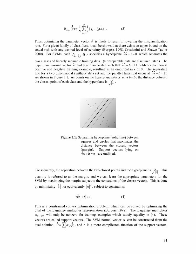
31

Remp (

r )

1

N

1

2i1

N

| yi f r (

rxi ) | . (3)

Thus, optimizing the parameter vector

is likely to result in lowering the misclassification

rate. For a given family of classifiers, it can be shown that there exists an upper bound on the actual risk with any desired level of certainty (Burgess 1998, Cristianini and Shawe-Taylor 2000). For SVMs, each

f r r

w,b ' (į ) specifies a hyperplane

rw

rx b 0 which separates the

two classes of linearly separable training data. (Nonseparable data are discussed later.) The hyperplane normal vector

rw and bias b are scaled such that

rw

rx b 1 holds for the closest

positive and negative training example, resulting in an empirical risk of 0. The separating line for a two dimensional synthetic data set and the parallel lines that occur at

rw

rx b 1

are shown in Figure 3.1. As points on the hyperplane satisfy rw

rx b 0 , the distance between

the closest point of each class and the hyperplane is 1 rw

.

Figure 3.1: Separating hyperplane (solid line) between squares and circles that maximizes the distance between the closest vectors (margin). Support vectors lying on rw

rx b 1 are outlined.

Consequently, the separation between the two closest points and the hyperplane is

2 rw

. This

quantity is referred to as the margin, and we can learn the appropriate parameters for the SVM by maximizing the margin subject to the constraints of the closest vectors. This is done

by minimizing

rw , or equivalently

rw

2, subject to constraints:

rw

rxi b 1. (4)

This is a constrained convex optimization problem, which can be solved by optimizing the dual of the Lagrange multiplier representation (Burgess 1998). The Lagrange multipliers

1 iN will only be nonzero for training examples which satisfy equality in (4). These

vectors are called support vectors. The SVM normal vector rw can be constructed from the

dual solution,

rw i

i yi

rxi , and b is a more complicated function of the support vectors,

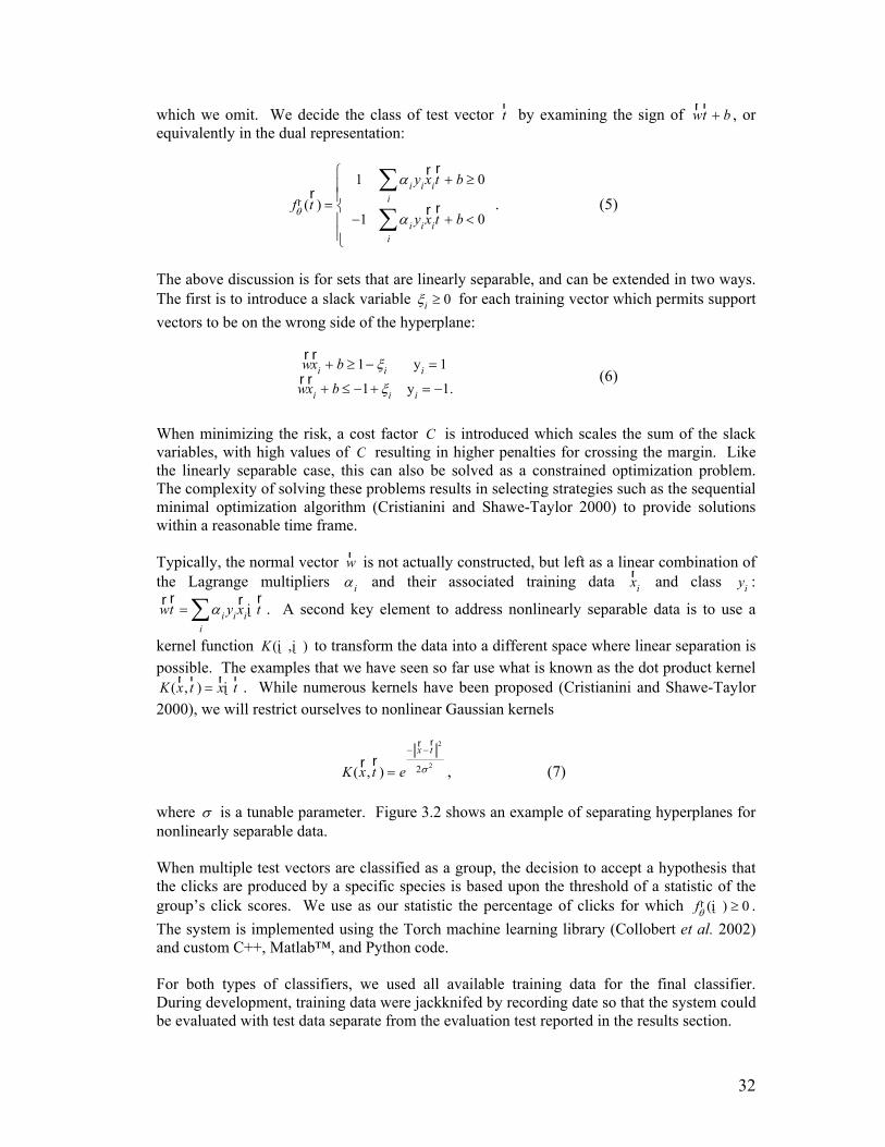
32

which we omit. We decide the class of test vector rt by examining the sign of

rw

rt b , or

equivalently in the dual representation:

f r (

rt )

1 ii yi

rxi

rt b 0

1 ii yi

rxi

rt b 0

. (5)

The above discussion is for sets that are linearly separable, and can be extended in two ways. The first is to introduce a slack variable i 0 for each training vector which permits support

vectors to be on the wrong side of the hyperplane:

rw

rxi b 1 i yi 1

rw

rxi b 1 i yi 1.

(6)

When minimizing the risk, a cost factor C is introduced which scales the sum of the slack variables, with high values of C resulting in higher penalties for crossing the margin. Like the linearly separable case, this can also be solved as a constrained optimization problem. The complexity of solving these problems results in selecting strategies such as the sequential minimal optimization algorithm (Cristianini and Shawe-Taylor 2000) to provide solutions within a reasonable time frame. Typically, the normal vector

rw is not actually constructed, but left as a linear combination of

the Lagrange multipliers i and their associated training data

rxi and class yi :

rw

rt i

i yi

rxiį

rt . A second key element to address nonlinearly separable data is to use a

kernel function K (į ,į ) to transform the data into a different space where linear separation is possible. The examples that we have seen so far use what is known as the dot product kernel

K (rx,

rt )

rxį

rt . While numerous kernels have been proposed (Cristianini and Shawe-Taylor

2000), we will restrict ourselves to nonlinear Gaussian kernels

K (rx,

rt ) e

rx

rt

2

2 2 , (7) where is a tunable parameter. Figure 3.2 shows an example of separating hyperplanes for nonlinearly separable data.

When multiple test vectors are classified as a group, the decision to accept a hypothesis that the clicks are produced by a specific species is based upon the threshold of a statistic of the group’s click scores. We use as our statistic the percentage of clicks for which f r

(į ) 0 .

The system is implemented using the Torch machine learning library (Collobert et al. 2002) and custom C++, Matlab™, and Python code. For both types of classifiers, we used all available training data for the final classifier. During development, training data were jackknifed by recording date so that the system could be evaluated with test data separate from the evaluation test reported in the results section.

33

Figure 3.2: Squares and circles that are not linearly separable. Hyperplane with dot product kernel (left) versus Gaussian kernel (right).

3.3.4: Evaluating results Results are plotted (Figures 3.3, 3.4) using the detection error tradeoff (DET) curve (Martin et al. 1997). DET curves are similar to receiver operator curves (ROC), except that in the former error rate normal deviates are plotted on both axes, whereas in the latter the correct detection and false alarm probabilities are plotted. When the false alarm and missed detection probabilities are normally distributed, the result is a straight line in DET space. DET plots are more effective at highlighting differences between similar systems than are ROC curves.

Results Mean normalized cepstral features were extracted for all files of the dataset. Tests on the jackknifed training data were used to tune the parameters of each classifier. For the GMMs, 2, 4, 8, 16, 32, and 64 mixture models were created, with 16 mixture models outperforming other parameters. For SVMs, a grid search on the penalty and standard deviation was performed (C{100, 200, …, 600}, {100, 200, …, 1000}). Equal error rates (EERs), the point at which a decision threshold results in the same percentage of false alarms (false positives) and missed detections, are summarized in Table 3.1. Tests on the last day’s training data performed poorly for SVMs, leading to the high overall EERs.

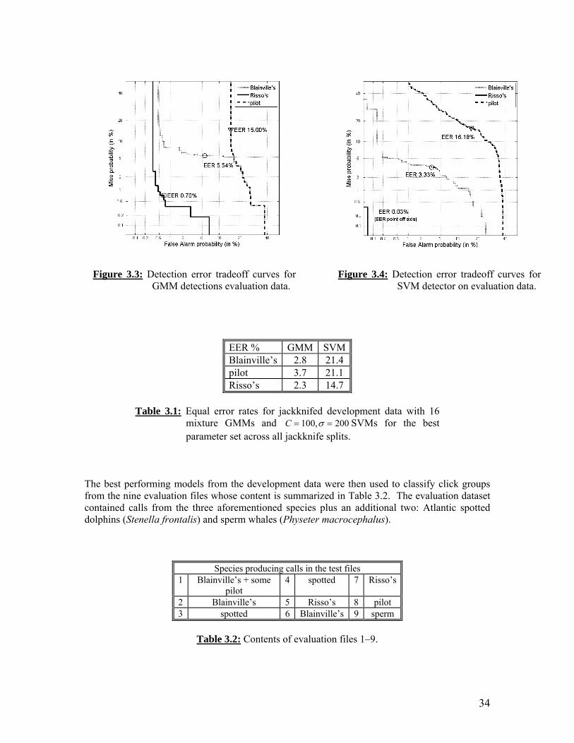
34

Figure 3.3: Detection error tradeoff curves for

GMM detections evaluation data.

Figure 3.4: Detection error tradeoff curves for

SVM detector on evaluation data.

EER % GMM SVMBlainville’s 2.8 21.4 pilot 3.7 21.1 Risso’s 2.3 14.7

Table 3.1: Equal error rates for jackknifed development data with 16

mixture GMMs and C 100, 200 SVMs for the best parameter set across all jackknife splits.

The best performing models from the development data were then used to classify click groups from the nine evaluation files whose content is summarized in Table 3.2. The evaluation dataset contained calls from the three aforementioned species plus an additional two: Atlantic spotted dolphins (Stenella frontalis) and sperm whales (Physeter macrocephalus).

Species producing calls in the test files 1 Blainville’s + some

pilot 4 spotted 7 Risso’s

2 Blainville’s 5 Risso’s 8 pilot 3 spotted 6 Blainville’s 9 sperm

Table 3.2: Contents of evaluation files 1–9.

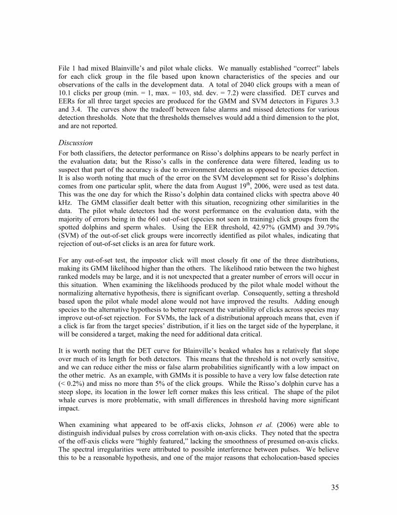
35

File 1 had mixed Blainville’s and pilot whale clicks. We manually established “correct” labels for each click group in the file based upon known characteristics of the species and our observations of the calls in the development data. A total of 2040 click groups with a mean of 10.1 clicks per group (min. = 1, max. = 103, std. dev. = 7.2) were classified. DET curves and EERs for all three target species are produced for the GMM and SVM detectors in Figures 3.3 and 3.4. The curves show the tradeoff between false alarms and missed detections for various detection thresholds. Note that the thresholds themselves would add a third dimension to the plot, and are not reported. Discussion For both classifiers, the detector performance on Risso’s dolphins appears to be nearly perfect in the evaluation data; but the Risso’s calls in the conference data were filtered, leading us to suspect that part of the accuracy is due to environment detection as opposed to species detection. It is also worth noting that much of the error on the SVM development set for Risso’s dolphins comes from one particular split, where the data from August 19th, 2006, were used as test data. This was the one day for which the Risso’s dolphin data contained clicks with spectra above 40 kHz. The GMM classifier dealt better with this situation, recognizing other similarities in the data. The pilot whale detectors had the worst performance on the evaluation data, with the majority of errors being in the 661 out-of-set (species not seen in training) click groups from the spotted dolphins and sperm whales. Using the EER threshold, 42.97% (GMM) and 39.79% (SVM) of the out-of-set click groups were incorrectly identified as pilot whales, indicating that rejection of out-of-set clicks is an area for future work. For any out-of-set test, the impostor click will most closely fit one of the three distributions, making its GMM likelihood higher than the others. The likelihood ratio between the two highest ranked models may be large, and it is not unexpected that a greater number of errors will occur in this situation. When examining the likelihoods produced by the pilot whale model without the normalizing alternative hypothesis, there is significant overlap. Consequently, setting a threshold based upon the pilot whale model alone would not have improved the results. Adding enough species to the alternative hypothesis to better represent the variability of clicks across species may improve out-of-set rejection. For SVMs, the lack of a distributional approach means that, even if a click is far from the target species’ distribution, if it lies on the target side of the hyperplane, it will be considered a target, making the need for additional data critical. It is worth noting that the DET curve for Blainville’s beaked whales has a relatively flat slope over much of its length for both detectors. This means that the threshold is not overly sensitive, and we can reduce either the miss or false alarm probabilities significantly with a low impact on the other metric. As an example, with GMMs it is possible to have a very low false detection rate (< 0.2%) and miss no more than 5% of the click groups. While the Risso’s dolphin curve has a steep slope, its location in the lower left corner makes this less critical. The shape of the pilot whale curves is more problematic, with small differences in threshold having more significant impact. When examining what appeared to be off-axis clicks, Johnson et al. (2006) were able to distinguish individual pulses by cross correlation with on-axis clicks. They noted that the spectra of the off-axis clicks were “highly featured,” lacking the smoothness of presumed on-axis clicks. The spectral irregularities were attributed to possible interference between pulses. We believe this to be a reasonable hypothesis, and one of the major reasons that echolocation-based species

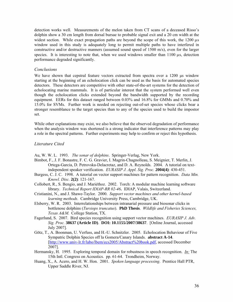
36

detection works well. Measurements of the melon taken from CT scans of a deceased Risso’s dolphin show a 30 cm length from dorsal bursae to probable signal exit and a 20 cm width at the widest section. While exact propagation paths are beyond the scope of this work, the 1200 s window used in this study is adequately long to permit multiple paths to have interfered in constructive and/or destructive manners (assumed sound speed of 1500 m/s), even for the larger species. It is interesting to note that, when we used windows smaller than 1100 s, detection performance degraded significantly. Conclusions We have shown that cepstral feature vectors extracted from spectra over a 1200 μs window starting at the beginning of an echolocation click can be used as the basis for automated species detectors. These detectors are competitive with other state-of-the-art systems for the detection of echolocating marine mammals. It is of particular interest that the system performed well even though the echolocation clicks extended beyond the bandwidth supported by the recording equipment. EERs for this dataset ranged between 0.03% and 16.8% for GMMs and 0.70% and 15.0% for SVMs. Further work is needed on rejecting out-of-set species whose clicks bear a stronger resemblance to the target species than to any of the species used to build the impostor set. While other explanations may exist, we also believe that the observed degradation of performance when the analysis window was shortened is a strong indicator that interference patterns may play a role in the spectral patterns. Further experiments may help to confirm or reject this hypothesis. Literature Cited

Au, W. W. L. 1993. The sonar of dolphins. Springer-Verlag, New York. Bimbot, F., J. F. Bonastre, F. C. G. Gravier, I. Magrin-Chagnolleau, S. Meignier, T. Merlin, J.

Ortega-Garcia, D. Petrovska-Delacretaz, and D. A. Reynolds. 2004. A tutorial on text-independent speaker verification. EURASIP J. Appl. Sig. Proc. 2004(4): 430-451.

Burgess, C. J. C. 1998. A tutorial on vector support machines for pattern recognition. Data Min. Knowl. Disc. 2(2): 121-167.

Collobert, R., S. Bengio, and J. Mariéthoz. 2002. Torch: A modular machine learning software library. Technical Report IDIAP-RR 02-46. IDIAP, Valais, Switzerland.

Cristianini, N., and J. Shawe-Taylor. 2000. Support vector machines and other kernel-based learning methods. Cambridge University Press, Cambridge, UK.

Elsberry, W. R. 2003. Interrelationships between intranarial pressure and biosonar clicks in bottlenose dolphins (Tursiops truncatus). PhD Thesis. Wildlife and Fisheries Sciences, Texas A&M. College Station, TX.

Fagerlund, S. 2007. Bird species recognition using support vector machines. EURASIP J. Adv. Sig. Proc. 38637 (Article ID). DOI: 10.1155/2007/38637. [Online Journal, accessed July 2007].

Götz, T., A. Boonman, U. Verfuss, and H.-U. Schnitzler. 2005. Echolocation Behaviour of Five Sympatric Dolphin Species off la Gomera/Canary Islands. abstract A-14. [http://www.univ-lr.fr/labo/lbem/ecs2005/Abstract%20book.pdf, accessed December 2007].

Hermansky, H. 1995. Exploring temporal domain for robustness in speech recognition. In: The 15th Intl. Congress on Acoustics. pp. 61-64. Trondheim, Norway.

Huang, X., A. Acero, and H. W. Hon. 2001. Spoken language processing. Prentice Hall PTR, Upper Saddle River, NJ.

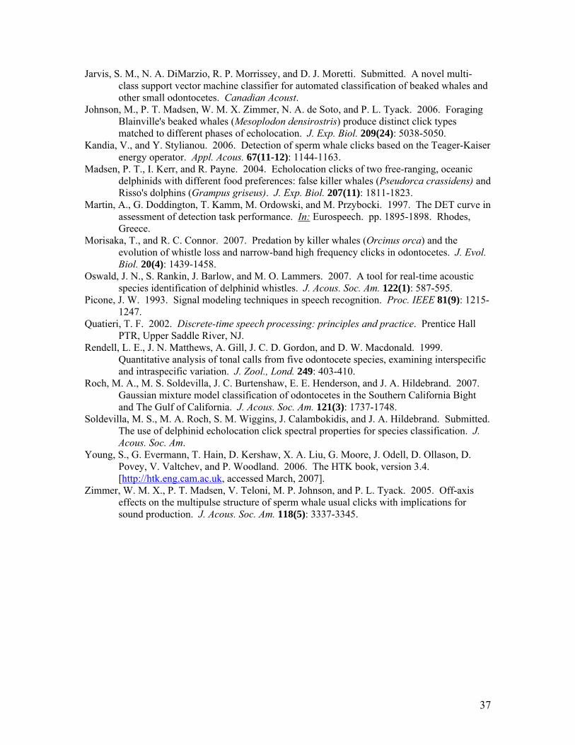
37

Jarvis, S. M., N. A. DiMarzio, R. P. Morrissey, and D. J. Moretti. Submitted. A novel multi-class support vector machine classifier for automated classification of beaked whales and other small odontocetes. Canadian Acoust.

Johnson, M., P. T. Madsen, W. M. X. Zimmer, N. A. de Soto, and P. L. Tyack. 2006. Foraging Blainville's beaked whales (Mesoplodon densirostris) produce distinct click types matched to different phases of echolocation. J. Exp. Biol. 209(24): 5038-5050.

Kandia, V., and Y. Stylianou. 2006. Detection of sperm whale clicks based on the Teager-Kaiser energy operator. Appl. Acous. 67(11-12): 1144-1163.

Madsen, P. T., I. Kerr, and R. Payne. 2004. Echolocation clicks of two free-ranging, oceanic delphinids with different food preferences: false killer whales (Pseudorca crassidens) and Risso's dolphins (Grampus griseus). J. Exp. Biol. 207(11): 1811-1823.

Martin, A., G. Doddington, T. Kamm, M. Ordowski, and M. Przybocki. 1997. The DET curve in assessment of detection task performance. In: Eurospeech. pp. 1895-1898. Rhodes, Greece.

Morisaka, T., and R. C. Connor. 2007. Predation by killer whales (Orcinus orca) and the evolution of whistle loss and narrow-band high frequency clicks in odontocetes. J. Evol. Biol. 20(4): 1439-1458.

Oswald, J. N., S. Rankin, J. Barlow, and M. O. Lammers. 2007. A tool for real-time acoustic species identification of delphinid whistles. J. Acous. Soc. Am. 122(1): 587-595.

Picone, J. W. 1993. Signal modeling techniques in speech recognition. Proc. IEEE 81(9): 1215-1247.

Quatieri, T. F. 2002. Discrete-time speech processing: principles and practice. Prentice Hall PTR, Upper Saddle River, NJ.

Rendell, L. E., J. N. Matthews, A. Gill, J. C. D. Gordon, and D. W. Macdonald. 1999. Quantitative analysis of tonal calls from five odontocete species, examining interspecific and intraspecific variation. J. Zool., Lond. 249: 403-410.

Roch, M. A., M. S. Soldevilla, J. C. Burtenshaw, E. E. Henderson, and J. A. Hildebrand. 2007. Gaussian mixture model classification of odontocetes in the Southern California Bight and The Gulf of California. J. Acous. Soc. Am. 121(3): 1737-1748.

Soldevilla, M. S., M. A. Roch, S. M. Wiggins, J. Calambokidis, and J. A. Hildebrand. Submitted. The use of delphinid echolocation click spectral properties for species classification. J. Acous. Soc. Am.

Young, S., G. Evermann, T. Hain, D. Kershaw, X. A. Liu, G. Moore, J. Odell, D. Ollason, D. Povey, V. Valtchev, and P. Woodland. 2006. The HTK book, version 3.4. [http://htk.eng.cam.ac.uk, accessed March, 2007].

Zimmer, W. M. X., P. T. Madsen, V. Teloni, M. P. Johnson, and P. L. Tyack. 2005. Off-axis effects on the multipulse structure of sperm whale usual clicks with implications for sound production. J. Acous. Soc. Am. 118(5): 3337-3345.

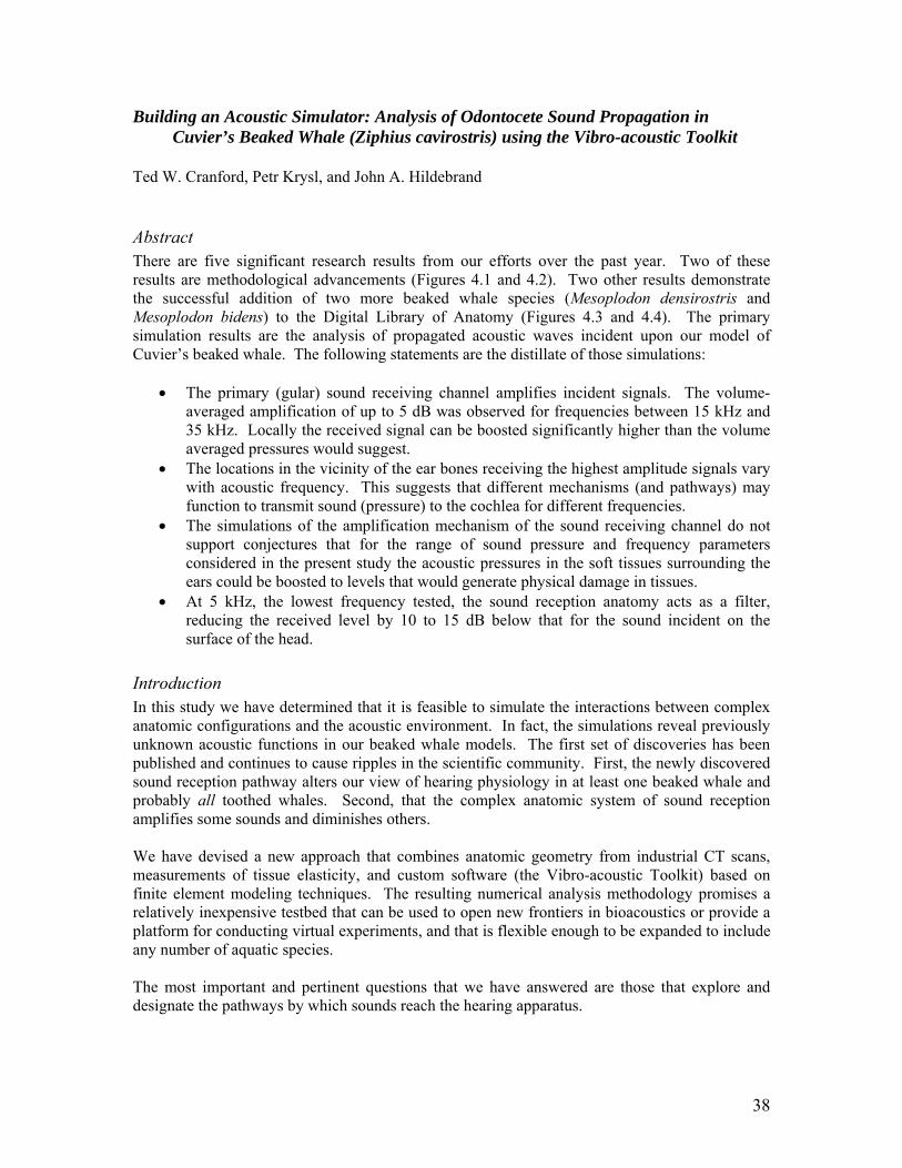
38

Building an Acoustic Simulator: Analysis of Odontocete Sound Propagation in Cuvier’s Beaked Whale (Ziphius cavirostris) using the Vibro-acoustic Toolkit

Ted W. Cranford, Petr Krysl, and John A. Hildebrand Abstract There are five significant research results from our efforts over the past year. Two of these results are methodological advancements (Figures 4.1 and 4.2). Two other results demonstrate the successful addition of two more beaked whale species (Mesoplodon densirostris and Mesoplodon bidens) to the Digital Library of Anatomy (Figures 4.3 and 4.4). The primary simulation results are the analysis of propagated acoustic waves incident upon our model of Cuvier’s beaked whale. The following statements are the distillate of those simulations:

The primary (gular) sound receiving channel amplifies incident signals. The volume-averaged amplification of up to 5 dB was observed for frequencies between 15 kHz and 35 kHz. Locally the received signal can be boosted significantly higher than the volume averaged pressures would suggest.

The locations in the vicinity of the ear bones receiving the highest amplitude signals vary with acoustic frequency. This suggests that different mechanisms (and pathways) may function to transmit sound (pressure) to the cochlea for different frequencies.

The simulations of the amplification mechanism of the sound receiving channel do not support conjectures that for the range of sound pressure and frequency parameters considered in the present study the acoustic pressures in the soft tissues surrounding the ears could be boosted to levels that would generate physical damage in tissues.

At 5 kHz, the lowest frequency tested, the sound reception anatomy acts as a filter, reducing the received level by 10 to 15 dB below that for the sound incident on the surface of the head.

Introduction In this study we have determined that it is feasible to simulate the interactions between complex anatomic configurations and the acoustic environment. In fact, the simulations reveal previously unknown acoustic functions in our beaked whale models. The first set of discoveries has been published and continues to cause ripples in the scientific community. First, the newly discovered sound reception pathway alters our view of hearing physiology in at least one beaked whale and probably all toothed whales. Second, that the complex anatomic system of sound reception amplifies some sounds and diminishes others. We have devised a new approach that combines anatomic geometry from industrial CT scans, measurements of tissue elasticity, and custom software (the Vibro-acoustic Toolkit) based on finite element modeling techniques. The resulting numerical analysis methodology promises a relatively inexpensive testbed that can be used to open new frontiers in bioacoustics or provide a platform for conducting virtual experiments, and that is flexible enough to be expanded to include any number of aquatic species. The most important and pertinent questions that we have answered are those that explore and designate the pathways by which sounds reach the hearing apparatus.

39

The simulations that address these questions have produced the most intriguing results and suggest a new pathway for sound reaching the ears. Our simulations suggest that for several frequencies tested in the vicinity of the frequency which the animals produce in the wild, a planar wave incident on the front of the animal propagates sound pressure waves along a novel pathway, entering the head from below and between the lower jaws. Sound then continues toward the bony ear complexes through the internal mandibular fat bodies. These and more recent results show that we have developed a powerful combination of techniques that provides a reliable, low-cost tool that can be used to investigate questions that probe the interaction between the complex anatomic structure of animals and a broad spectrum of sound sources. The value of this technological triumph increases with the expanding taxonomic breadth of the digital library of cetacean anatomy. Finite element modeling also facilitates acoustic investigations on a broad spectrum of non-mammalian vertebrates. Methodology In order to accomplish discretization of anatomic geometry (Cranford et al. 2008b), we developed a voxel-based mesh from x-ray CT data, combined it with measurements of tissue elasticity, and added a comprehensive formulation for vibro-acoustic problems (Cranford et al. 2008a, Krysl et al. 2007). The Vibro-acoustic Toolkit contains a fully Lagrangian finite element formulation based on the decomposition of incident and scattered fields that has been developed to incorporate seamless coupling of fluids and viscoelastic solids, and to allow for accurate representation of incident acoustic excitation (Krysl et al. 2007). This highly efficient parallel finite element code runs on an eight processor Linux machine that allows numerical simulations with ~1/2 billion unknowns to be calculated within a matter of days. Summary of Results

Methodological Advancements

This project has pushed out the frontiers of our research on many fronts. One of the primary developments has been the demonstration of the ability to CT scan large whales. We have scanned large specimens half a dozen times over the course of this project and continue to refine and improve the associated methodological processes. In the past year we have accomplished two methodological advancements. The first allows us to take advantage of economies of scale. We added a twist on the method of CT scanning large specimens to allow for scanning multiple specimens simultaneously. Figure 4.1 shows two views of a reconstruction from CT scans of five beaked whale specimens, all having been scanned at the same time. The long slender rods are composed of known density material for facilitating 3-D reconstructions and density comparisons (Cranford et al. 2008b).

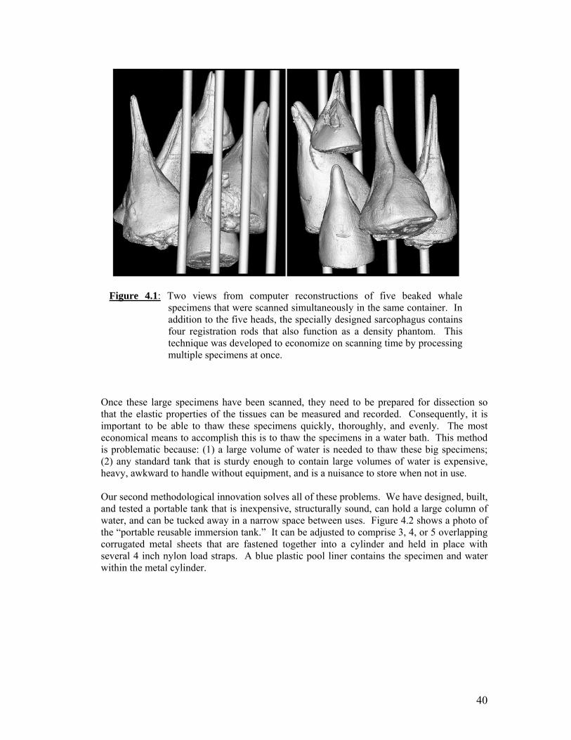
40

Figure 4.1: Two views from computer reconstructions of five beaked whale

specimens that were scanned simultaneously in the same container. In addition to the five heads, the specially designed sarcophagus contains four registration rods that also function as a density phantom. This technique was developed to economize on scanning time by processing multiple specimens at once.

Once these large specimens have been scanned, they need to be prepared for dissection so that the elastic properties of the tissues can be measured and recorded. Consequently, it is important to be able to thaw these specimens quickly, thoroughly, and evenly. The most economical means to accomplish this is to thaw the specimens in a water bath. This method is problematic because: (1) a large volume of water is needed to thaw these big specimens; (2) any standard tank that is sturdy enough to contain large volumes of water is expensive, heavy, awkward to handle without equipment, and is a nuisance to store when not in use. Our second methodological innovation solves all of these problems. We have designed, built, and tested a portable tank that is inexpensive, structurally sound, can hold a large column of water, and can be tucked away in a narrow space between uses. Figure 4.2 shows a photo of the “portable reusable immersion tank.” It can be adjusted to comprise 3, 4, or 5 overlapping corrugated metal sheets that are fastened together into a cylinder and held in place with several 4 inch nylon load straps. A blue plastic pool liner contains the specimen and water within the metal cylinder.

41

Figure 4.2: Portable reusable immersion tank. This chamber is used to thaw large frozen whale heads evenly and thoroughly so that they can be dissected. The cylindrical chamber is constructed of overlapping corrugated metal panels that hold a swimming pool liner and is retained with a series of nylon load straps. Between usages the chamber can be disassembled and stored in a relatively compact space.

Additions to the Digital Library of Anatomy

We have added new sets of scans from the Blainville’s beaked whale (Mesoplodon densirostris) and Sowerby’s beaked whale (Mesoplodon bidens) to the Digital Library of Anatomy (Figures 4.3 and 4.4). These scans have been segmented and the specimens dissected at the National Museum of Natural History. This accomplishment will allow us to use finite element modeling studies to compare the functional anatomy of three species in the Digital Library of Anatomy (Blainville’s beaked whale, Sowerby’s beaked whale, and Cuvier’s beaked whale) to test whether there are significant differences that might account for the greater number of strandings that occur by Cuvier’s beaked whale in the presence of high intensity sound. Preparations for these tests are underway.

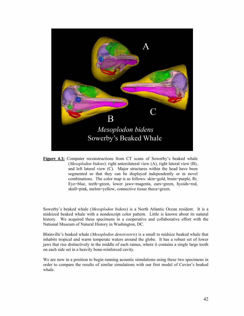
42

Figure 4.3: Computer reconstructions from CT scans of Sowerby’s beaked whale (Mesoplodon bidens): right anterolateral view (A), right lateral view (B), and left lateral view (C). Major structures within the head have been segmented so that they can be displayed independently or in novel combinations. The color map is as follows: skin=gold, brain=purple, Rt. Eye=blue, teeth=green, lower jaws=magenta, ears=green, hyoids=red, skull=pink, melon=yellow, connective tissue theca=green.

Sowerby’s beaked whale (Mesoplodon bidens) is a North Atlantic Ocean resident. It is a midsized beaked whale with a nondescript color pattern. Little is known about its natural history. We acquired these specimens in a cooperative and collaborative effort with the National Museum of Natural History in Washington, DC. Blainville’s beaked whale (Mesoplodon densirostris) is a small to midsize beaked whale that inhabits tropical and warm temperate waters around the globe. It has a robust set of lower jaws that rise distinctively in the middle of each ramus, where it contains a single large tooth on each side set in a heavily bone-reinforced cavity. We are now in a position to begin running acoustic simulations using these two specimens in order to compare the results of similar simulations with our first model of Cuvier’s beaked whale.

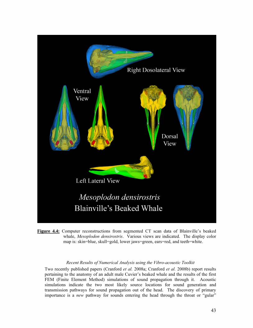
43

Figure 4.4: Computer reconstructions from segmented CT scan data of Blainville’s beaked

whale, Mesoplodon densirostris. Various views are indicated. The display color map is: skin=blue, skull=gold, lower jaws=green, ears=red, and teeth=white.

Recent Results of Numerical Analysis using the Vibro-acoustic Toolkit

Two recently published papers (Cranford et al. 2008a; Cranford et al. 2008b) report results pertaining to the anatomy of an adult male Cuvier’s beaked whale and the results of the first FEM (Finite Element Method) simulations of sound propagation through it. Acoustic simulations indicate the two most likely source locations for sound generation and transmission pathways for sound propagation out of the head. The discovery of primary importance is a new pathway for sounds entering the head through the throat or “gular”

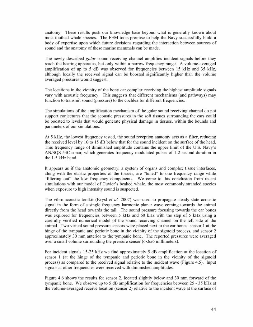
44

anatomy. These results push our knowledge base beyond what is generally known about most toothed whale species. The FEM tools promise to help the Navy successfully build a body of expertise upon which future decisions regarding the interaction between sources of sound and the anatomy of these marine mammals can be made. The newly described gular sound receiving channel amplifies incident signals before they reach the hearing apparatus, but only within a narrow frequency range. A volume-averaged amplification of up to 5 dB was observed for frequencies between 15 kHz and 35 kHz, although locally the received signal can be boosted significantly higher than the volume averaged pressures would suggest. The locations in the vicinity of the bony ear complex receiving the highest amplitude signals vary with acoustic frequency. This suggests that different mechanisms (and pathways) may function to transmit sound (pressure) to the cochlea for different frequencies. The simulations of the amplification mechanism of the gular sound receiving channel do not support conjectures that the acoustic pressures in the soft tissues surrounding the ears could be boosted to levels that would generate physical damage in tissues, within the bounds and parameters of our simulations. At 5 kHz, the lowest frequency tested, the sound reception anatomy acts as a filter, reducing the received level by 10 to 15 dB below that for the sound incident on the surface of the head. This frequency range of diminished amplitude contains the upper limit of the U.S. Navy’s AN/SQS-53C sonar, which generates frequency-modulated pulses of 1-2 second duration in the 1-5 kHz band. It appears as if the anatomic geometry, a system of organs and complex tissue interfaces, along with the elastic properties of the tissues, are “tuned” to one frequency range while “filtering out” the low frequency components. We come to this conclusion from recent simulations with our model of Cuvier’s beaked whale, the most commonly stranded species when exposure to high intensity sound is suspected. The vibro-acoustic toolkit (Krysl et al. 2007) was used to propagate steady-state acoustic signal in the form of a single frequency harmonic planar wave coming towards the animal directly from the head towards the tail. The sound pressure focusing towards the ear bones was explored for frequencies between 5 kHz and 60 kHz with the step of 5 kHz using a carefully verified numerical model of the sound receiving channel on the left side of the animal. Two virtual sound pressure sensors were placed next to the ear bones: sensor 1 at the hinge of the tympanic and periotic bone in the vicinity of the sigmoid process, and sensor 2 approximately 30 mm anterior to the tympanic bone. The reported pressures were averaged over a small volume surrounding the pressure sensor (6x6x6 millimeters). For incident signals 15-25 kHz we find approximately 5 dB amplification at the location of sensor 1 (at the hinge of the tympanic and periotic bone in the vicinity of the sigmoid process) as compared to the received signal relative to the incident wave (Figure 4.5). Input signals at other frequencies were received with diminished amplitudes. Figure 4.6 shows the results for sensor 2, located slightly below and 30 mm forward of the tympanic bone. We observe up to 5 dB amplification for frequencies between 25 - 35 kHz at the volume-averaged receive location (sensor 2) relative to the incident wave at the surface of

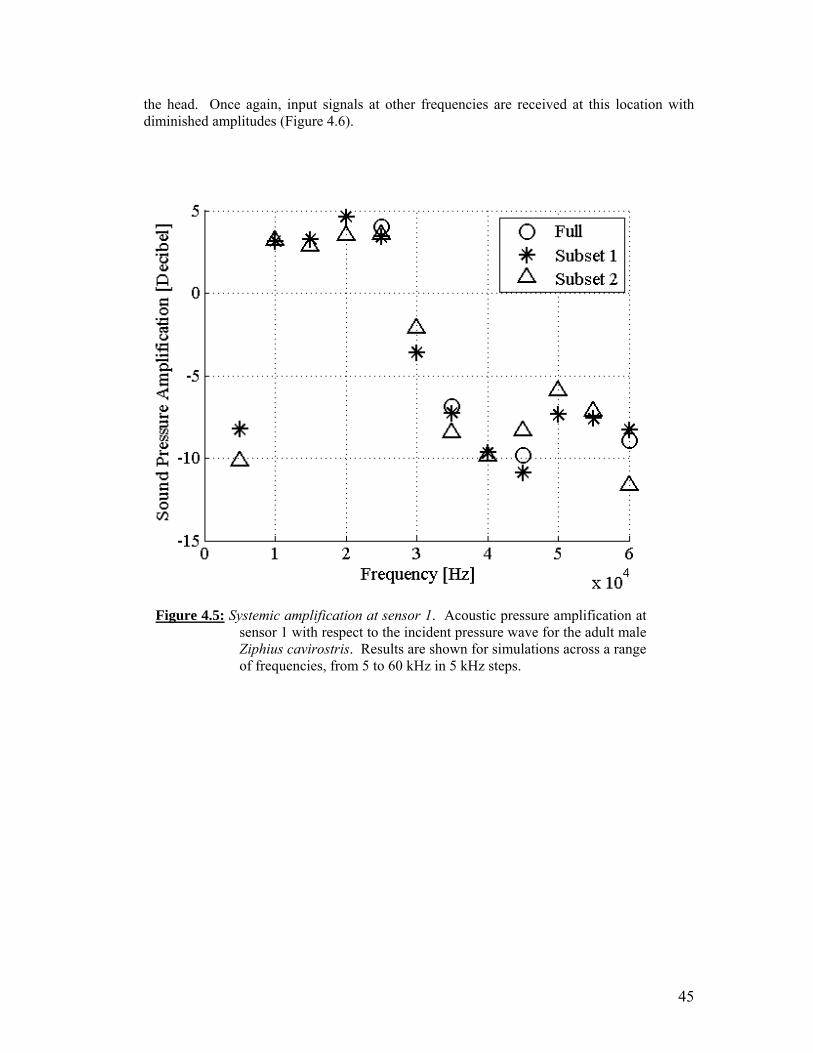
45

the head. Once again, input signals at other frequencies are received at this location with diminished amplitudes (Figure 4.6).

Figure 4.5: Systemic amplification at sensor 1. Acoustic pressure amplification at sensor 1 with respect to the incident pressure wave for the adult male Ziphius cavirostris. Results are shown for simulations across a range of frequencies, from 5 to 60 kHz in 5 kHz steps.

46

Figure 4.6: Systemic amplification at sensor 2. Acoustic pressure amplification at sensor 2 with respect to the incident pressure wave for the adult male Ziphius cavirostris. Results are shown for simulations across a range of frequencies, from 5 to 60 kHz in 5 kHz steps.

Future Plans

Anatomic Studies

Launch a parallel FEM simulation effort using the bottlenose dolphin (Tursiops truncatus) in order to evaluate and validate current methodological practices and results.

Develop a FEM simulation of sound propagation from the environment through the head

to the bony tympanoperiotic (hearing) complex in our model of Cuvier’s beaked whale. Develop vibrational analysis tools to simulate the vibrational characteristics of the bony

tympanoperiotic (hearing) complex in a bottlenose dolphin based on existing CT scans. Develop instrumentation to measure shear-wave velocity in tissue samples, then set up a

test tank in which to immerse the mandible from the same Cuvier’s beaked whale we used to build our numerical analysis model (Cranford et al. 2008b). This apparatus will allow us to evaluate our latest “flexural wave” hypothesis for sound propagation along the conventional pathway to the odontocete ear complex (Norris 1968).

47

Future Directions in Vibro-acoustic Research

The results obtained with the current selection of finite elements do not display any pathologies associated with zero-frequency rotation modes, spurious acoustic modes, or locking in the incompressible limit; yet these weaknesses are commonly encountered in Lagrangian finite element codes. No theoretical proofs that these elements will perform satisfactorily are available at this point. This deficiency should be corrected to ensure that the implementation is a robust and reliable tool. Along these lines, we have published a paper on finite elements that addresses behavior in the incompressible limit. We haven't solved the question of whether our current elements are subject to spurious acoustic modes. The approximation of surfaces of general shape does contain some error in the present implementation: surfaces are approximated by the faces of the voxels, hence are jagged even when the actual surfaces are perfectly smooth. Some artifacts of the special orientation of the voxel computational grid may be visible in the results, especially the pressure. This could become a critical issue when dealing with the hearing of beaked whales, since the ear bones and other structures around the ears are very delicate, and a good representation of the surfaces (or, put another way, of the acoustic impedances at the interfaces that these surfaces represent) may be required. We have made some headway on a technique for improving jagged geometry approximations. A paper was submitted to demonstrate technology for modeling shear-locking-free plates, which are a crucial ingredient for the next step, which is models for locking-free shells. With the shell model we want to address the representation of thin bones by embedding the shells in the tissue voxels as a replacement of the 3-D hard bone. Initial investigations will be undertaken to achieve a multi-scale resolution of the acoustic/mechanical waves, so that the entire animal can eventually be exposed to sound while at the same time detailed results may be obtained around a very small feature, such as the ear bones. We have formulated the basic strategy for addressing the problem by decomposing the response of the local model in terms of the incident waves (computed with the global model) and a perturbation due to the difference in resolution between the global and local model. We are currently working on the formulation details and the implementation.

Literature Cited

CALAMBOKIDIS, J. and J. BARLOW. 2004. Abundance of blue and humpback whales in the

eastern north Pacific estimated by capture-recapture and line-transect methods. Marine Mammal Science 20: 63-85.

CRANFORD, T. W., P. KRYSL, and J. A. HILDEBRAND. 2008a. Sound pathways revealed: Simulated sound transmission and reception in Cuvier’s beaked whale (Ziphius cavirostris). Bioinsp. Biomim. 3: 1-10.

CRANFORD, T. W., M. F. MCKENNA, M. S. SOLDEVILLA, S. M. WIGGINS, R. E. SHADWICK, J. GOLDBOGEN, P. KRYSL, J. A. ST. LEGER, and J. A. HILDEBRAND. 2008b. Anatomic geometry of sound transmission and reception in Cuvier's beaked whale (Ziphius cavirostris). Anatomical Record 291: 353-378.

FORNEY, K. A. and J. BARLOW. 1998. Seasonal patterns in the abundance and distribution of California cetaceans, 1991-1992. Marine Mammal Science 14: 460-489.

FORNEY, K. A., J. BARLOW, and J. V. CARRETTA. 1995. The Abundance of Cetaceans in California Waters .2. Aerial Surveys in Winter and Spring of 1991 and 1992. Fishery Bulletin 93: 15-26.

48

GREEN, G., J. J. BRUEGGEMAN, R. A. GROTEFENDT, C. E. BOWLBY, M. L. BONNELL, and I. K. C. BALCOMB. 1992. Cetacean distribution and abundance off Oregon and Washington. Ch. 1. Oregon and Washington Marine Mammal and Seabird Surveys.OCS Study 91-0093. Final Report prepared for: Pacific OCS Region, Minerals 120 Management Service,. U.S. Department of the Interior, Los Angeles, California.

HEYNING, J. E. and W. F. PERRIN. 1994. Evidence for two species of common dolphins (Genus Delphinus) from the eastern North Pacific. Pages 1-35. Contributions in Science. Natural History Museum, L.A. County.

KRYSL, P., T. W. CRANFORD, and J. A. HILDEBRAND. 2007. Lagrangian finite element treatment of transient vibration/acoustics of biosolids immersed in fluids. Int. J. Numer. Meth. Engng. DOI: 10.1002/nme.2192.

LARKMAN, V. E. and R. R. VEIT. 1998. Seasonality and Abundance of Blue Whales off Southern California. CalCOFI Reports 39: 236-239.

NORRIS, K. S. 1968. The evolution of acoustic mechanisms in odontocete cetaceans. Pages 297-324. In: E. T. DRAKE (ed.) Evolution and Environment. Yale University Press, New Haven.

POOLE, M. M. 1984. Migration corridors of gray whales (Eschrichtius robustus) along the central California coast, 1980-1982. Pages 389-407. In: JONES M. L., S. L. SWARTZ and S. LEATHERWOOD (eds.). The Gray Whale. Academic Press, New York.

49

Project Publications

Peer Reviewed Publications CRANFORD, T. W., P. KRYSL, and J. A. HILDEBRAND. 2008. Acoustic pathways revealed:

simulated sound transmission and reception in Cuvier’s beaked whale (Ziphius cavirostris) using the vibro-acoustic toolkit. Bioinspiration and Biomimetics 3 (10pp). DOI: 10.1088/1748-3182/3/1/016001 (Published online).

CRANFORD, T. W., P. KRYSL, and J. A. HILDEBRAND. 2008. Anatomic geometry of sound

transmission and reception in Cuvier's beaked whale (Ziphius cavirostris). Anatomical Record 291:353-378.

JOHNSTON, D. W., M. MCDONALD, J. POLOVINA, R. DOMOKOS, S. WIGGINS, AND J.

HILDEBRAND. 2008. Temporal patterns in the acoustic signals of beaked whales at Cross Seamount. Biology Letters 4(2): 208-211.

KRYSL, P., T. W. CRANFORD, and J. A. HILDEBRAND. 2008. Lagrangian finite element treatment

of transient vibration/acoustics of biosolids immersed in fluids. International Journal for Numerical Methods in Engineering 74(5): 754-775.

MADHUSUDHANA, S. K., E. M. OLESON, M. S. SOLDEVILLA, M. A. ROCH, AND J. A.

HILDEBRAND. 2008. Frequency based algorithm for robust contour extraction of blue whale B and D calls. OCEANS 2008-MTS/IEEE Kobe Techno-Ocean: 1-8.

MCDONALD, M. A., J. A. HILDEBRAND, S. M. WIGGINS, AND D. ROSS. 2008. A fifty year

comparison of ambient ocean noise near San Clemente Island: a bathymetrically complex coastal region off southern California. J. Acoust. Soc. Am. 124(4): 1985-1992.

MCKENNA M. F., J. A. GOLDBOGEN, J. S. LEGER, J. A. HILDEBRAND, T. W. CRANFORD. 2007.

Evaluation of postmortem changes in tissue structure in the bottlenose dolphin (Tursiops truncatus). Anatomical Record 290(8):1023-1032.

OLESON, E. M., S. M. WIGGINS, AND J. A. HILDEBRAND. 2007. Temporal separation of blue

whale call types on a southern California feeding ground. Animal Behaviour 74: 881-894.

ROCH, M. A., M. S. SOLDEVILLA, R. HOENIGMAN, S. M. WIGGINS, AND J. A. HILDEBRAND.

2008. Comparison of machine learning techniques for the classification of echolocation clicks from three species of odontocetes. Canadian Acoustics 36(1):41-47.

SOLDEVILLA, M. S., E. E. HENDERSON, G. S. CAMPBELL, S. M. WIGGINS, J. A. HILDEBRAND, AND

M. A. ROCH. 2008. Classification of Risso's and Pacific white-sided dolphins using spectral properties of echolocation clicks. J. Acoust. Soc. Am. 124(1): 609-624.

50

WIGGINS, S. M. AND J. A. HILDEBRAND. 2007. High-frequency Acoustic Recording Package (HARP) for broad-band, long-term marine mammal monitoring. Pages 551-557. International Symposium on Underwater Technology 2007 and International Workshop on Scientific Use of Submarine Cables & Related Technologies 2007. Institute of Electrical and Electronics Engineers, Tokyo, Japan.

Abstracts BAUMANN, S., J. A. HILDEBRAND, S. M. WIGGINS, AND .U. H. SCHNITZLER. 2008. Species

identification and measurement of activity in odontocete species of Palmyra Atoll by acoustic monitoring. J Acoust Soc Am 123(5): 3099.

BERCHOK, C. L., G. L. D’SPAIN, AND J. A. HILDEBRAND. 2007. Tracking baleen whales using

the relative relocation method. J. Acoust. Soc. Am. 122: 3003. CRANFORD, T.W., P. KRYSL, AND J.A. HILDEBRAND. 2007. Sound propagation in Cuvier’s

beaked whale (Ziphius cavirostris): A test case for simulating sound propagation in aquatic organisms using FEM. Conference on the Effects of Noise on Aquatic Life. Nyborg, Denmark.

CRANFORD, T.W., P. KRYSL, AND J.A. HILDEBRAND. 2007. Sound pathways revealed: simulated

sound transmission and reception in Ziphius cavirostris. 17th Biennial Conference on the Biology of Marine Mammals. Cape Town, South Africa.

HENDERSON, E. E., J. A. HILDEBRAND, J. BARLOW, K. A. FORNEY, J. CALAMBOKIDIS, AND A. B.

DOUGLAS. 2008. Do climate regime shifts alter occurrence patterns of marine mammals in the Southern California Bight? ASLO CalCOFI Conference. (March 2008)

KIM, K., P. HURSKY, M. B. PORTER, J. A. HILDEBRAND, E. HENDERSON, J. CALAMBOKIDIS, AND

E. FALCONE. 2008. Acoustic studies of dolphins in their natural habitat: Challenges and successes. J Acoust Soc Am 123(5): 3363.

MADHUSUDHANA, S. K., E. M. OLESON, M. S. SOLDEVILLA, M. A. ROCH, J. A HILDEBRAND.

2008. Blue whale B and D call extraction and classification using a frequency domain based robust contour extractor. Passive '08. (14-17 October 2008).

OLESON, E. M., M. S. SOLDEVILLA, J. CALAMBOKIDIS, C. COLLINS, S. M. WIGGINS, AND J. A.

HILDEBRAND. 2008. Distribution patterns of delphinids in the California Current Ecosystem observed through acoustic monitoring of species-specific echolocation clicks. J Acoust Soc Am 123(5): 3099.

OLESON, E. M., S. M. WIGGINS, AND J. A. HILDEBRAND. 2007. The impact of non-continuous

sampling on cetacean acoustic detection probability, presented at the 3rd International Workshop on the Detection and Classification of Marine Mammals Using Passive Acoustics. Boston, MA. (24-26 July, 2007).

ROCH, M. A., H. KLINCK, D. K. MELLINGER, M. S. SOLDEVILLA, AND J. A. HILDEBRAND. 2008.

Comparison of feature extraction methods for the identification of odontocete species based upon echolocation clicks. J Acoust Soc Am 123(5): 3100.

51

ROCH, M. A., M. S. SOLDEVILLA, J. C. BURTENSHAW, R. HOENIGMAN, S. M. WIGGINS, J. A.

HILDEBRAND. 2007. Comparison of machine learning techniques for the classification of echolocation clicks from three species of odontocetes, presented at the 3rd International Workshop on the Detection and Classification of Marine Mammals Using Passive Acoustics. Boston, MA. (24-26 July, 2007).

SOLDEVILLA, M. S., J. A. HILDEBRAND, S. M. WIGGINS, AND M. A. ROCH. 2008. Long-term

passive acoustic monitoring of delphinids in the Southern California Bight. J Acoust Soc Am 123(5): 3101.

SOLDEVILLA, M. S., M. A. ROCH, S. M. WIGGINS, J. A. HILDEBRAND. 2007. Spatial and

Temporal patterns in delphinid calling bouts offshore of southern California, presented at the 3rd International Workshop on the Detection and Classification of Marine Mammals using Passive Acoustics, Boston, MA. (July 24-26, 2007).

SOLDEVILLA, M., S. WIGGINS, E. OLESON, N. RUBIO, M. OHMAN, R. DAVIS, M. KAHRU, AND J.

HILDEBRAND. 2008. Cetacean habitat modeling in the California Current System. ASLO CalCOFI Conference. (March 2008)

52

Initial Distribution List

1. 2. 3. 4. 5. 6. 7. 8. 9. 10.

Defense Technical Information Center 8725 John J. Kingman Rd., STE 0944 Ft. Belvoir, VA 22060-6218 Dudley Knox Library, Code 013 Naval Postgraduate School Monterey, CA 93943-5100 Erin Oleson National Marine Fisheries Service Pacific Islands Fisheries Science Center Honolulu, HI John Hildebrand Scripps Institution of Oceanography University of California La Jolla, CA John Calambokidis Cascadia Research Collective Olympia, WA Greg Schorr Cascadia Research Collective Olympia, WA Erin Falcone Cascadia Research Collective Olympia, WA Ching-Sang Chiu Naval Postgraduate School Monterey, CA Curtis A. Collins Naval Postgraduate School Monterey, CA Thomas A. Rago Naval Postgraduate School Monterey, CA

2 2 1 1 1 1 1 1 1 1

53

11. 12. 13. 14. 15. 16. 17. 18. 19. 20. 21.

Tetyana Margolina Naval Postgraduate School Monterey, CA Chris Miller Naval Postgraduate School Monterey, CA John Joseph Naval Postgraduate School Monterey, CA Katherine Whitaker Pacific Grove, CA Frank Stone CNO(N45) Washington, D.C. Jay Barlow Southwest Fisheries Science Center, NOAA La Jolla, CA CAPT Ernie Young, USN (Ret.) CNO(N45) Washington, D.C. Dale Liechty CNO(N45) Washington, D.C. Dave Mellinger Oregon State University Newport, OR Kate Stafford Applied Physics Laboratory University of Washington Seattle, CA Sue Moore NOAA at Applied Physics Laboratory University of Washington Seattle, WA

1 1 1 1 1 1 1 1 1 1 1

54

22. 23. 24. 25. 26. 27. 28. 29. 30. 31.

Petr Krysl University of California La Jolla, CA Mark McDonald Whale Acoustics Bellvue, CO Ted Cranford Quantitative Morphology Consulting, Inc. AND San Diego State University San Diego, CA Monique Fargues Naval Postgraduate School Monterey, CA Mary Ann Daher Woods Hole Oceanographic Institution Woods Hole, MA Heidi Nevitt NAS North Island San Diego, CA Rebecca Stone Naval Postgraduate School Monterey, CA Melissa Hock Scripps Institution of Oceanography University of California La Jolla, CA Sean M. Wiggins Scripps Institution of Oceanography University of California La Jolla, CA E. Elizabeth Henderson Scripps Institution of Oceanography University of California La Jolla, CA

1 1 1 1 1 1 1 1 1 1

55

32. 33. 34. 35. 36. 37. 38. 39. 40. 41. 42.

Gregory S. Campbell Scripps Institution of Oceanography University of California La Jolla, CA Marie A. Roch San Diego State University San Diego, CA Anne Douglas Cascadia Research Collective Olympia, WA Julie Rivers Naval Facilities Engineering Command, Pacific Pearl Harbor, HI Jenny Marshall Naval Facilities Engineering Command San Diego, CA Chip Johnson COMPACFLT Pearl Harbor, HI CDR Len Remias U.S. Pacific Fleet Pearl Harbor, HI LCDR Robert S. Thompson U.S. Pacific Fleet Pearl Harbor, HI Jene J. Nissen U. S. Fleet Forces Command Norfolk, VA W. David Noble U. S. Fleet Forces Command Norfolk, VA David T. MacDuffee U. S. Fleet Forces Command Norfolk, VA

1 1 1 1 1 1 1 1 1 1 1

56

43. 44. 45. 46. 47. 48. 49. 50. 51. 52. 53.

Keith A. Jenkins Naval Facilities Engineering Command, Atlantic Norfolk, VA Joel T. Bell Naval Facilities Engineering Command, Atlantic Norfolk, VA Mandy L. Shoemaker Naval Facilities Engineering Command, Atlantic Norfolk, VA Anurag Kumar Naval Facilities Engineering Command, Atlantic Norfolk, VA Merel Dalebout University of New South Wales Sydney, Australia Robin W. Baird Cascadia Research Collective Olympia, WA Brenda K. Rone National Marine Mammal Laboratory Seattle, WA Phil Clapham National Marine Mammal Laboratory Seattle, WA Laura J. Morse National Marine Mammal Laboratory Seattle, WA Anthony Martinez NOAA Southeast Fisheries Science Center Miami, FL Darlene R. Ketten Woods Hole Oceanographic Institution Woods Hole, MA

1 1 1 1 1 1 1 1 1 1 1

57

54. 55. 56. 57. 58. 59. 60.

David C. Mountain Boston University Boston, MA Melissa Soldevilla Duke University Durham, NC Lisa Munger Scripps Institution of Oceanography University of California La Jolla, CA Karlina Merkens Scripps Institution of Oceanography University of California La Jolla, CA Andrea Havron Spatial Ecosystems Olympia, WA Dominique Camacho Spatial Ecosystems Olympia, WA Rhonda Hoenigman University of Colorado Boulder, CO

1 1 1 1 1. 1. 1.