Embed Size (px)
Citation preview

AD-A263 512
NAVAL POSTGRADUATE SCHOOLMonterey, California
DTIC~EL 1993THESIS S MAY o 3 1993
SWAY, YAW, AND ROLL COUPLING EFFECTS ON
STRAIGHT LINE STABILITY OF SUBMERSIBLES
by
Daniel J. Cunningham, II
March, 1993
Thesis Advisor: Fotis A. Papoulias
Approved for public release; distribution is unlimited
93-09293
93 4 61 0`6

REPORT DOCUMENTATION PAGE Form ApprovedOMB No 0704-0188
Public reOtring .uromnf •Or thi roi'ectiOn of ,nformat.O' s% • ,nal. o i c af a ge'3qn u Oe' .e•DCrfe ,'C ud,'O te ,,e rc, repi Pse" S'c. ? 3a ':,. -. - -e• i P ,ggathering and mnaintaining Ite data needed. and co'psetinQ and ree..ng 1fr 3lierjiori of r,nl(Crmatio. Sena Cynn'eris 'ela'a.-g t .'n rnuEC3collemEon of into(Mtnion, ncluding suggestions for reducing this ourder, ic Washinglon Heaod ,arIer,% Servces Direcorate 0o, nitcr•a-on OiDeai.-, ,no Rp0 ,r ¾ 5 e• ,,es,Danrs Hrgtr.ay. Swte 12D4, Arlington,. vd 222024302 afld c Inn Off-? ot kManageer'in aria uadge! Paoe,.c'n Reo,,-in-n 'CleAm Q'C'4 0'880 ', $ I ýZ' --:- ,2ý
1. AGENCY USE ONLY (Leave blank) 2. REPORT DATE 3. REPORT TYPE AND DATES COVERED
Imarch 1993 ,Master's Thesis4. TITLE AND SUBTITLE 5. FUNDING NUMBERS
Sway, Yaw, and Roll Coupling Effects onStraight Line Stability of Submersibles
6. AUTHOR(S)
Cunringham, DIniel J. II
7. PERFORMING ORGANIZATION NAME(S) AND AODRESS(ES) 8. PERFORMING ORGANIZATION
Naval [ostgraduate School REPORT NUMBER
Monterey, California 93943-5000
9. SPONSORING/MONITORING AGENCY NAME(S) AND ADDRESS(ES) 10. SPONSORING/MONITORINGAGENCY REPORT NUMBER
11. SUPPLEMENTARY NOTES
The views expressed in this thesis are those of the author and do not reflect theofficial policy or position of the Department of Defense or the U.S. government.
12a. DISTRIBUTION /AVAILABILITY STATEMENT 12b. DISTRIBUTION CODE
Apprved for public release; distribution is unlimited.
13. ABSTRACT (Maximum 200 words)
This thesis analyzes the sway, yaw, and roll dynamic stability of neutrallybuoyant submersibles. Utilizing the hydrodynamic coefficients for a Mark IXSwimmer Delivery Vehicle (SDV) as a base-line model, the linearized equations ofmotion for the decoupled steering and roll system are compared to the coupledsystem. To different configurations of hydrodynamic coefficients are consideredalong with the effects of varying the vertical (Z}) and longitudinal (X ) centersof gravity of the vehicle hdile the longitudinal denter of buoyancy (Xby is heldconstant. Results demonstrate the significant effects on stability of couplingthe steering and roll equations of motion, and the upiortance of Zg and Xg selectionin minimizing those effects while retaining stability. Perturbati6n analysisresults confirm the essential dependence of the linearized coupled equations on the
* separation of xg. and x1b.
14. SUBJECT TERMS 15. NUMBER OF PAGES
Straight Line Stability of Neutrally Buoyant Submersibles; 84Dynmuic Wbupling; Submersibles; Steering and Roll Equations 16. PRICE CODE
17. SECURITY CLASSIFICATION 18. SECURITY CLASSIFICATION 19. SECURITY CLASSIFICATION 20. LIMITATION OF ABSTRACTOF REPORT OF THIS PAGE OF ABSTRACT
Uclassified Unclassified Unl]assified ULNSN 7540-01-280-SS00 Standard Form 298 (Rev 2-89)
Prescribed by ANS Sld 139-18

Approved for public release; distribution is unlimited.
Sway, Yaw, and Roll Coupling Effects on
Straight Line Stability of Submersibles
by
Daniel J. Cunningham, IILieutenant, United States Navy
B.A., The University of Vermont, 1983
Submitted in partial fulfillment of therequirements for the degree of
MASTER OF SCIENCE IN MECHANICAL ENGINEERING
from the
NAVAL POSTGRADUATE SCHOOL
March, 1993
Author: '9--'..\ -•Daniel #L\Cunninghain, II
Approved by: 1s2"6sdvisoFoji- apouliais, Thesis Advisor
l~tthew D. Kelleher, ChairmanDepartment of Mechanical Engineering
ii
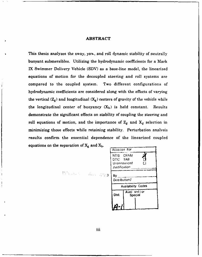
ABSTRACT
This thesis analyzes the sway, yaw, and roll dynamic stability of neutrally
buoyant submersibles. Utilizing the hydrodynamic coefficients for a Mark
IX Swimmer Delivery Vehicle (SDV) as a base-line model, the linearized
equations of motion for the decoupled steering and roll systems are
compared to the coupled system. Two different configurations of
hydrodynamic coefficients are considered along with the effects of varying
the vertical (Zg) and longitudinal (Xg) centers of gravity of the vehicle while
the longitudinal center of buoyancy (Xb) is held constant. Results
demonstrate the significant effects on stability of coupling the steering and
roll equations of motion, and the importance of Zg and Xg selection in
minimizing those effects while retaining stability. Perturbation analysis
results confirm the essential dependence of the linearized coupled
equations on the separation of Xg and Xb.Accesion For
NTIS CRA•&IrTTIC TAB
IUnannounced CJustifica tion . ............. ......... .
S. . . .. .:t : . . 7.:j 3 B y .. . . . . .......... . . . . . .
Distribution/I
Availability 'Codes'
' Avail and I or
Dist Special
TABLE OF CONTENTS
I. INTRODUCTION ..................................................................... 1
A. GENERAL ................................................................................................... 1
B. PARAMETER DEFINITION .............................................................. 2
1. Variables .......................................................................................... 3
II. STABILITY OF MOTION .......................................................... 6
A. EQUATIONS OF MOTION ................................................................. 6
B. SIMPLIFICATIONS ............................................................................ 7
C. COUPLED STABILITY EQUATIONS ............................................ 8
D. UNCOUPLED STABILITY EQUATIONS ..................................... 10
IIL RESULTS AND DISCUSSION .............................................. . 12
A. DEGREE OF STABILITY ................................................................... 12
B. REGIONS OF STABILITY ................................................................ 12
C., INTERPRETATION OF RESULTS .................................................. 18
D. 7 LINEAR SIMULATIONS ................................................................... 24
E. NON-LINEAR SIMULATIONS ...................................................... 35
IV. PitiTURBATION ANALYSIS .......................... .................. . 48
A.' BACKGROUND ................................................................................... 48
B..... PERTURBATION FORMULATION ............................................... 48
V. CONCLUSIONS AND RECOMMENDATIONS .......................... 61
iv
APPENDIX A. NON-LINEAR SIMULATION PROGRAM .......... 62
LINEAR SIMULATION PROGRAM ................ 67
CROSSFLOW INTEGRAL PROGRAM ............ 69
EIGENVALUE CALCULATION PROGRAM ...... 69
FIRST AND SECOND ORDER PERTURBATIONAPPROXIMATION COMPUTER PROGRAM ..... 71
LIST OF REFERENCES ................................................................. 74
BIBLIOGRAPHY ........................................................................ 74
INITIAL DISTRIBUTION LIST ...................................................... 75
v
LIST OF FIGURES
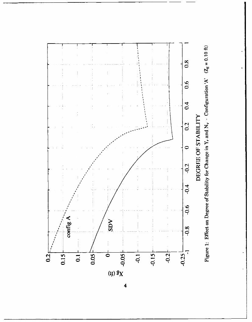
Figure 1: Effect on Degree of Stability for Change in Yr and N,for Configuration 'A' ...................................................................... 4
Figure 2: Effect on Degree of Stability for Change in Yr and N,for Configuration 'B' ....................................................................... 5
Figure 3: Effects of Xg and Zg on Degree of Stability forConfiguration 'A' ............................................................................... 13
Figure 4: Effects of Xg and Zg on Imaginary Part of Root forConfiguration 'A' ............................................................................ 14
Figure 5: Effects of Xg and Zg on Degree of Stability forConfiguration 'B' ............................................................................ 15
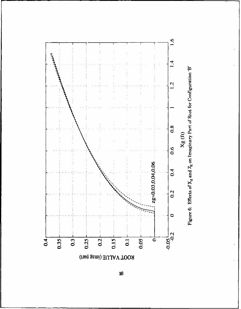
Figure 6: Effects of Xg and Zg on Imaginary Part of Root for
Configuration 'S ' ............................................................................. 16
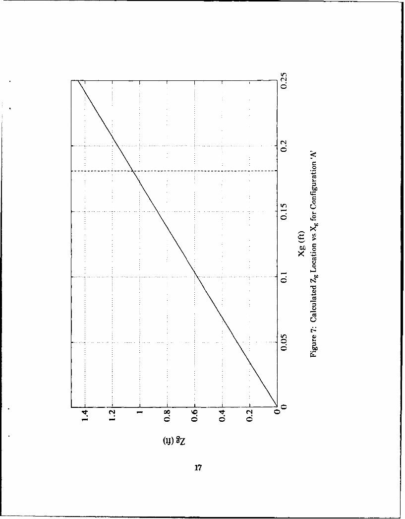
Figure 7: Calculated Zg Location vs Xg for Configuration 'A' ............... 17
Figure 8: Calculated Zg Location vs Xg for Configuration 'B' ......... 19
Figure 9a: Effects of Xg and Zg on Degree of Stability when XbEquals Xg for Configuration ' ............................................... 2D
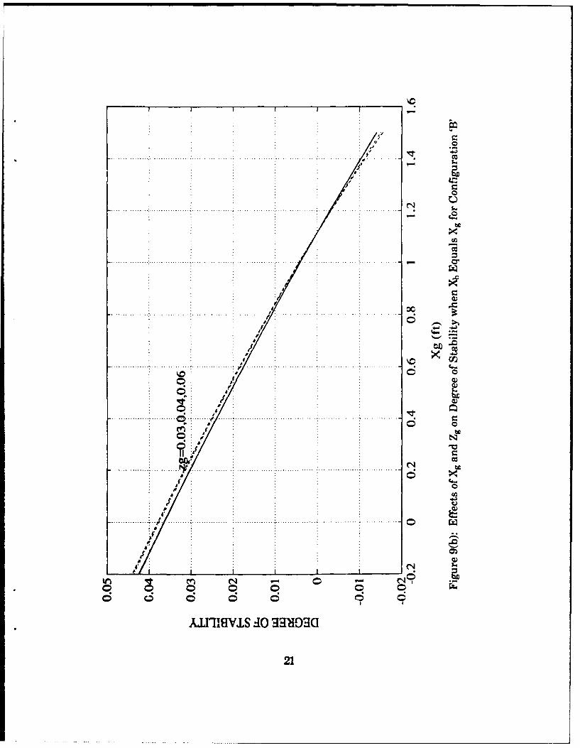
Figure 9b: Effects of Xg and Zg on Degree of Stability when XbEquals Xg for Configuration 'B' .................................................... 21
Figure 10: Normalized Routh Criterion Values vs Xg forVarying Zg Values - Configuration 'B' .................. 23
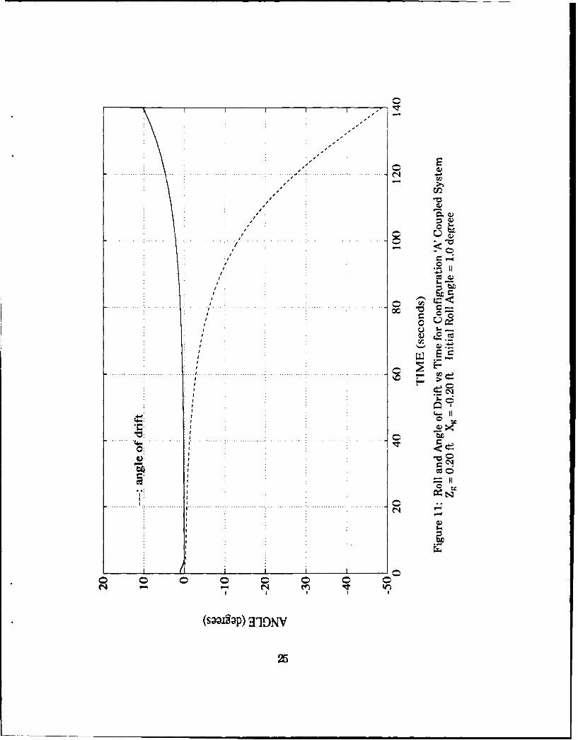
Figure 11: Roll and Angle of Drift vs Time for Configuration 'A'Coupled System - Unstable ......................................................... 25
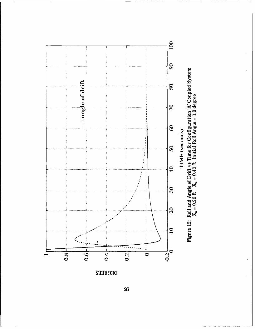
Figure 12: Roll and Angle of Drift vs Time for Configuration 'A'Coupled System - Stable ............................................................... 26
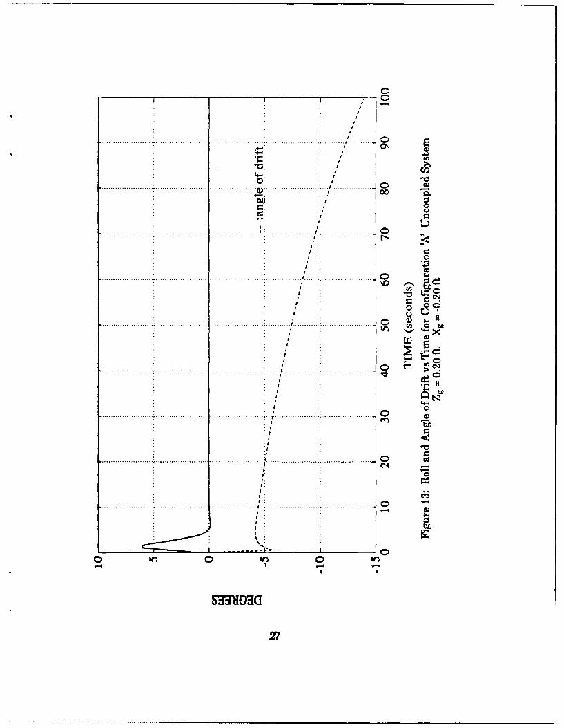
Figure 13: Roll and Angle of Drift vs Time for Configuration 'A'Uncoupled System - Unstable ........................................................ 27
vi
Figure 14: Roll and Angle of Drift vs Time for Configuration 'A'Uncoupled System - Stable .............................................................. 28
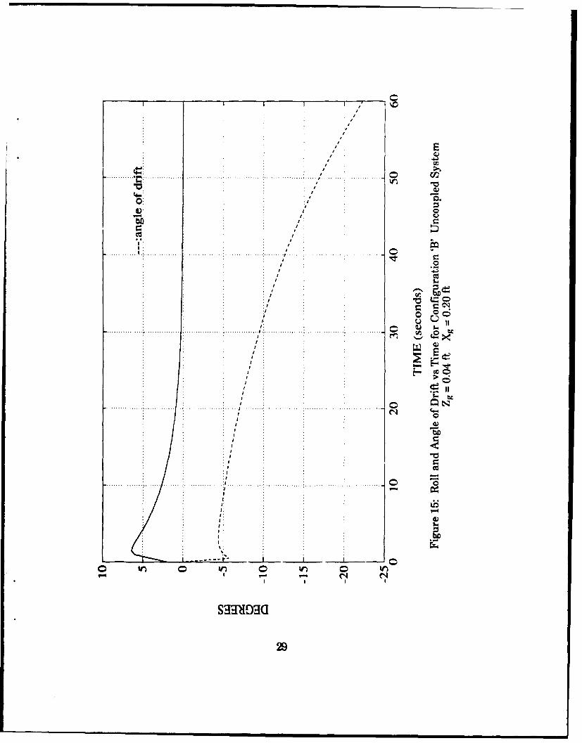
Figure 15: Roll and Angle of Drift vs Time for Configuration 'B'Uncoupled System - Xg = 0.20 ft .................................................. 29
Figure 16: Roll and Angle of Drift vs Time for Configuration 'B'Uncoupled System - Xg = 1.00 ft .................................................. 30
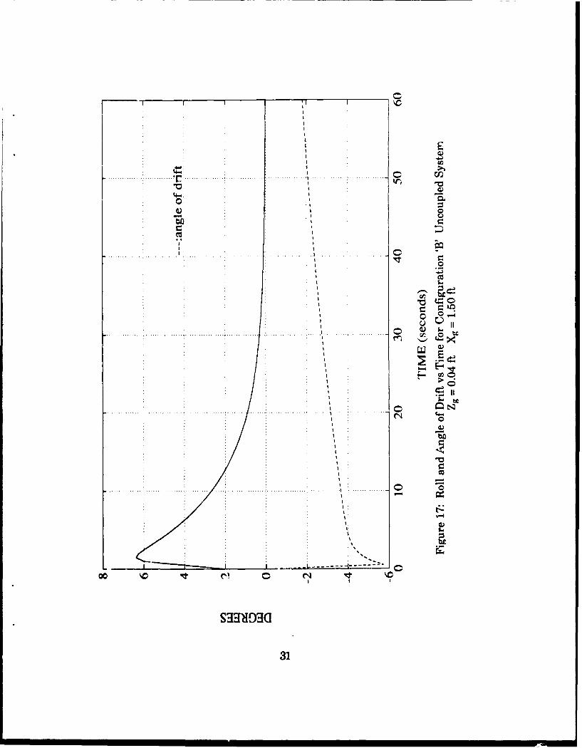
Figure 17: Roll and Angle of Drift vs Time for Configuration 'B'Uncoupled System - Xg = 1.50 ft .................................................. 31
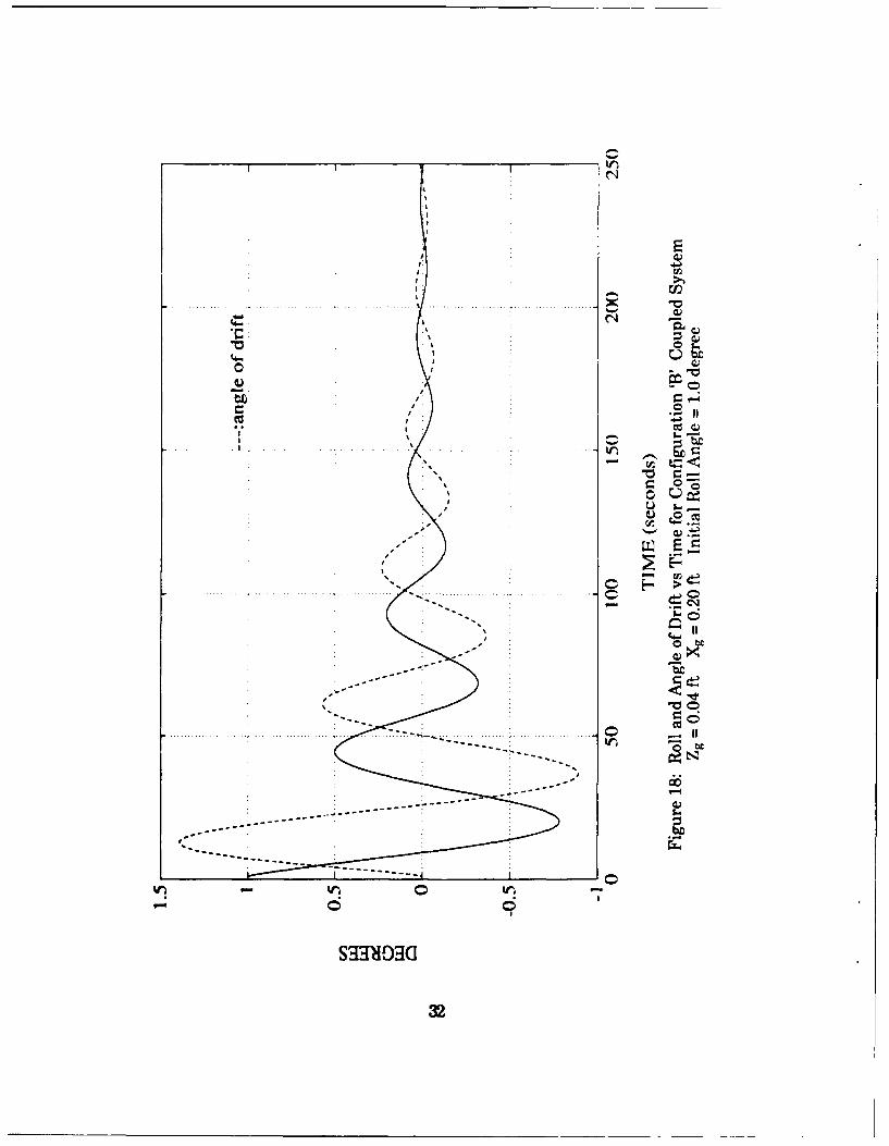
Figure 18: Roll and Angle of Drift vs Time for Configuration 'B'Coupled System - Xg = 0.20 ft ........................................................... 32
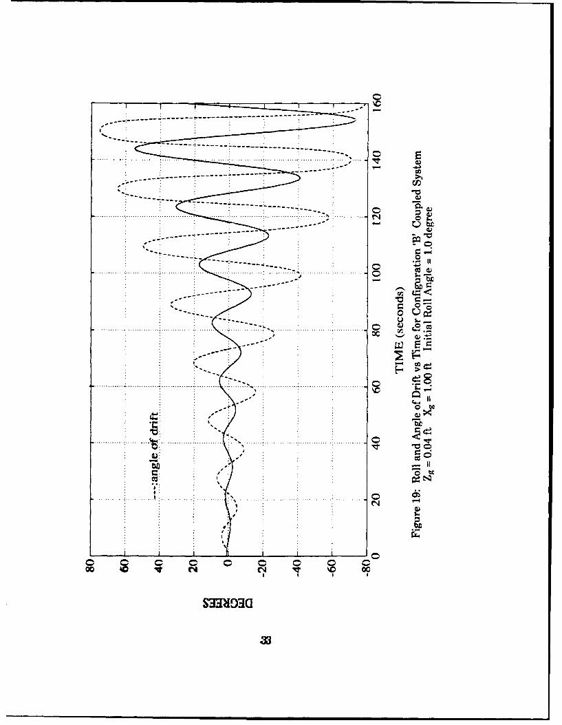
Figure 19: Roll and Angle of Drift vs Time for Configuration 'B'Coupled System - Xg = 1.00 ft ....................................................... 33
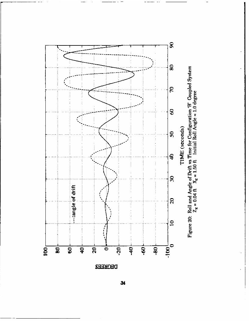
Figure 20: Roll and Angle of Drift vs Time for Configuration 'B'Coupled System - Xg = 1.50 ft ....................................................... 34
Figure 21: Mesh Plot of Roll Angle vs Time for Configuration 'B'as Xg varies from 0.15 to 1.50 ft ................................................... 36
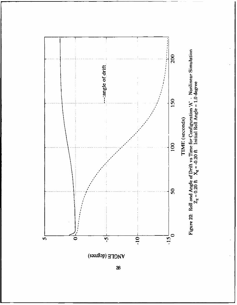
Figure 22: Roll and Angle of Drift vs Time for Configuration 'A'Nonlinear Simulation - Xg = -0.20 ft .......................................... 38
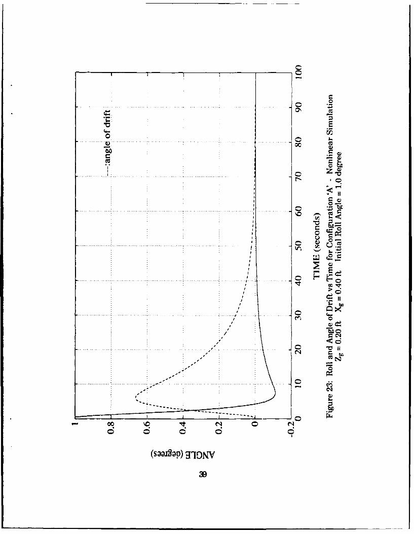
Figure 23: Roll and Angle of Drift vs Time for Configuration 'A'Nonlinear Simulation - Xg = 0.40 ft ............................................ 39
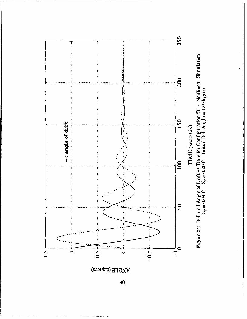
Figure 24: Roll and Angle of Drift vs Time for Configuration 'B'Nonlinear Simulation - Xg = 0.20 ft ............................................ 40
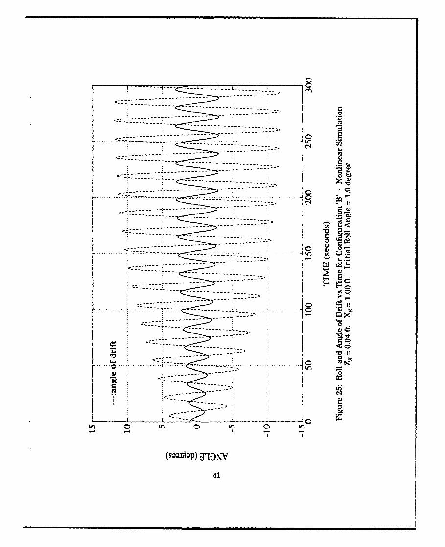
Figure 25: Roll and Angle of Drift vs Time for Configuration 'B'Nonlinear Simulation - Xg = 1.00 ft ............................................ 41
Figure 26: Roll Angle vs Time Comparison Between Linear andNonlinear Simulations for Configuration 'B' ; Xg = 1.00 ft ..... 42
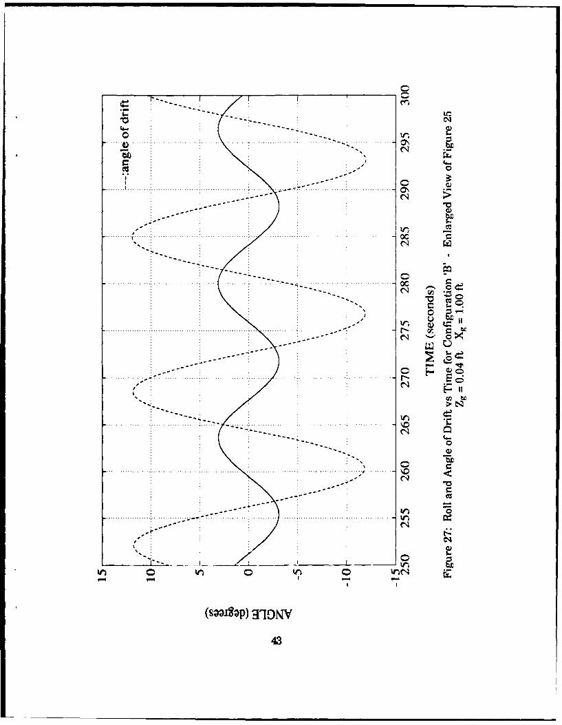
Figure 27: Roll and Angle of Drift vs Time for Configuration 'B'Enlarged View of Figure 25; Xg = 1.00 ft .................................. 43
vii
Figure 28: LilmL Cycle Phase Plane Trajectory for Roll Angle vsAngle of Drift - Configuration 'B'; Xg = 1.00 ft ......................... 44
Figure 29: Roll and Angle of Drift vs Time for Configuration 'B' withConstant Zero-Mean Sway and Yaw Disturbances ............... 47
Figure 30: Comparison of Degree of Stability vs Xg with Six CrossCoupling Coefficients Neglected - Configuration 'A' ............ 51
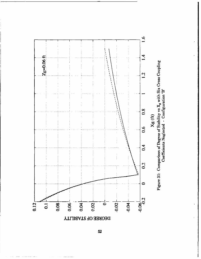
Figure 31: Comparison of Degree of Stability vs Xg with Six CrossCoupling Coefficients Neglected - Configuration 'B'......... 52
Figure 32: Comparison of Degree of Stability vs Xg Neglecting HigherOrder Terms of Xg and Zg - Configuration 'A' ............ 54
Figure 33: Comparison of Degree of Stability vs Xg Neglecting HigherOrder Terms of Xg and Zg - Configuration 'B' ......................... 55
Figure 34: First Order Perturbation Approximation forConfiguration 'A' ............................................................................ 57
Figure 35: First Order Perturbation Approximation forConfiguration B' ............................................................................... 58
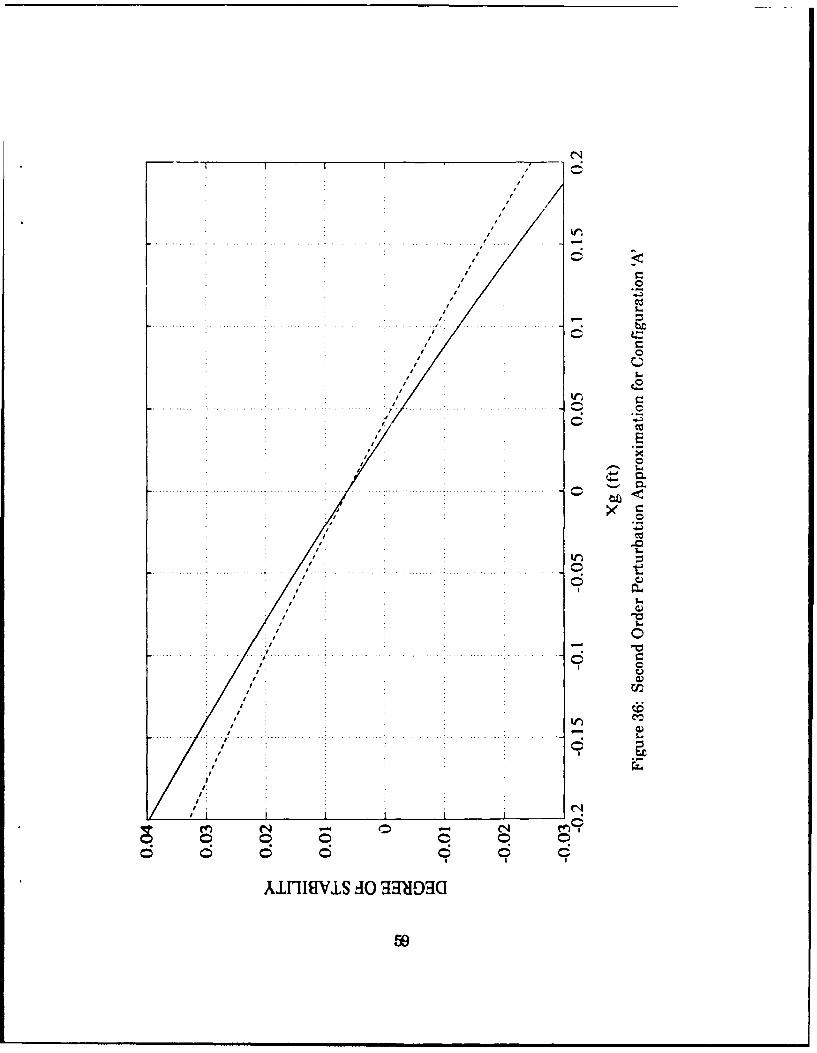
Figure 36: Second Order Perturbation Approlimation forConfiguration 'A' ........................................................................ 59
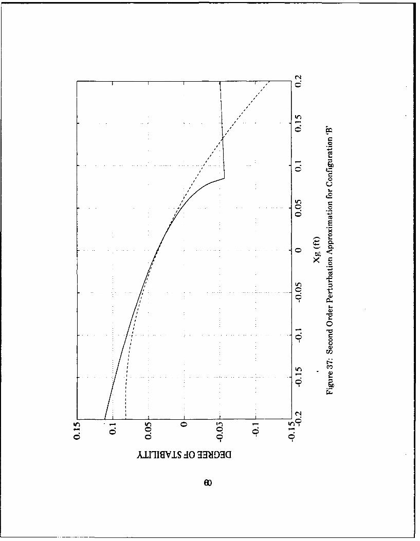
Figure 37: Second Order Perturbation Approximation forConfiguration B' ......................................................................... 60
viii
I. INTRODUCTION
A. GENERAL
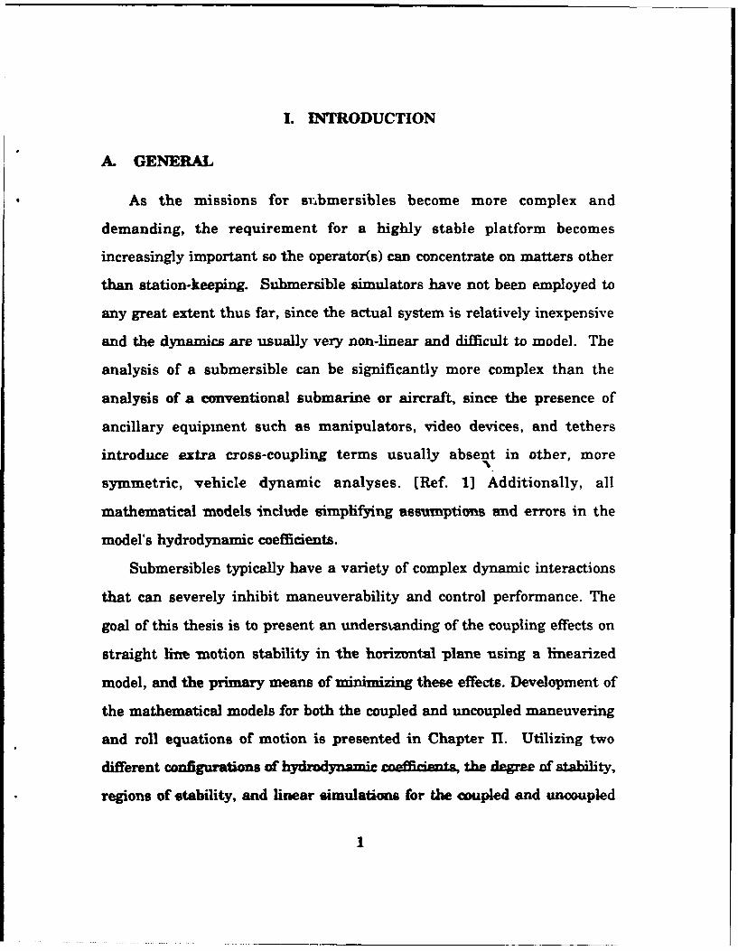
As the missions for si:,bmersibles become more complex and
demanding, the requirement for a highly stable platform becomes
increasingly important so the operator(s) can concentrate on matters other
than station-keeping. Submersible simulators have not been employed to
any great extent thus far, since the actual system is relatively inexpensive
and the dynamics are usually very non-linear and difficult to model. The
analysis of a submersible can be significantly more complex than the
analysis of a conventional submarine or aircraft, since the presence of
ancillary equipment such as manipulators, video devices, and tethers
introduce extra cross-coupling terms usually absent in other, more
symmetric, vehicle dynamic analyses. [Ref. 1] Additionally, all
mathematical models include simplifying assumptions and errors in the
model's hydrodynamic coefficients.
Submersibles typically have a variety of complex dynamic interactions
that can severely inhibit maneuverability and control performance. The
goal of this thesis is to present an understanding of the coupling effects on
straight line -motion stability in the horizontal plane using a linearized
model, and the primary means of minimizing these effects. Development of
the mathematical models for both the coupled and uncoupled maneuvering
and roll equations of motion is presented in Chapter fl. Utilizing two
different configurations of hy ami coeffiaents, the degree of stability,
regions of stability, and linear oimulations for the coupled and uncoupled
1

systems are presented in Chapter III. A Hamming method nonlinear
simulation [Ref. 2], which is similar to a fourth order Runge-Kutta
integration technique, is conducted on both configurations to compare with
the results obtained for the linearized models. Chapter IV develops a
perturbation analysis to demonstrate the strong degree of dependence on
the separation between the longitudinal centers of buoyancy and gravity to
the solution of the linearize%-- coupled equations of motion. Chapter V
summarizes the results and provides recommendations for future
submersible modelling research. Appendix A contains the computer
programs utilized for the lip iar and nonlinear simulations.
B. PARAMETER DEFINITION
The values for the hydrodynamic derivatives and vehicle dimensions
are from Smith, Crane, and Summey [Ref. 3], with the following exceptions:
"* Yr - the force in sway due to a change in yaw rate
" N, - the moment due to a change in sway velocity.
These two coefficients were modified to produce two different models that
would have one eigenvalue change sign for a reasonable range of
longitudinal and vertical centers of gravity. A comparison between the
actual non-dimensional values and those used in this thesis is as follows:
oi a ' -0 24EConfiguration 'A' -3.500F,02 -1.484F-03
Configuration 'B' -5.940E-02 -1.484E-03
Actual SDV 2.970E-02 -7.420E-03
2
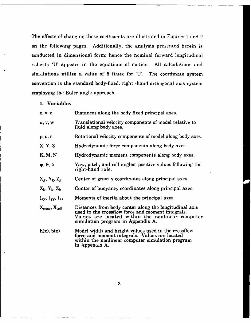
The effects of changing these coefficients are illustrated in Figures 1 and 2
on the following pages. Additionally, the analysis prebented herein is
conducted in dimensional form; hence the nominal forward longitudinal
vNeI)zity 'U' appears in the equations of motion. All calculations and
simulations utilize a value of 5 ft/sec for 'U'. The coordinate system
convention is the standard body-fixed, right -hand orthogonal axis system
employing the Euler angle approach.
1. Variables
x, y, z Distances along the body fixed principal axes.
u, v, w Translational velocity components of model relative tofluid along body axes.
p, q, r Rotational velocity components of model along body axes.
X, Y, Z Hydrodynamic force components along body axes.
K, M, N Hydrodynamic moment components along body axes.
Y e, ' Yaw, pitch, and roll angles; positive values following theright-hand rule.
Xg, Yg, Zg Center of gravi' y coordinates along principal axes.
Xb, Yb, Zb Center of buoyancy coordinates along principal axes.
IXX, Iyy, IZZ Moments of inertia about the principal axes.
Xno", Xtail Distances from body center along the longitudinal axisused in the crossflow force and moment integrals.Values are located within the nonlinear computersimulation program in Appendix A.
h(x), b(x) Model width and height values used in the crossflowforce and moment integrals. Values are locatedwithin the nonlinear computer simulation programin Appenix A.
3
I c
* :I
* I
CC
000........ ... r zy
'/ . /
II)
0) 0
4

II
.. .. .... ... .. .......... ..... .. .. . .
S.. ... . . .. ... . .• . . . ... .. . . ' . ... . . . .. " " . . . . . . .. ... . .. . .. . . .. .. . . . . . . . .. ..
¶ .
40
• I -
S.. . . . . . . . . . . . . . . . . . .... .. .. .. .. . t '". ....... . ... . .. .. . .. .. .. ... .. .. . .. .. . . ... ... . .. .. .. . . ... .....
~ a
ocz
. . . . .. .......
S.. . . . . . . . . . . . . . ....... ............... . . . . . . ...................... .. . . ... . . . . . o
5 0 5
6 16
to)
(U 2

II. STABILITY OF MOTION
A. EQUATIONS OF MOTION
The horizontal plane, nonlinear equations of motion for a submersible
as developed by Smith, Crane, and Summey [Ref. 1] are shown below in
Equations (2.1).
Sway: m[V+ ur-wp±Xg(pq + j) yg(p2 + r2) +Zg(qr-p)](2.1a)[YpP+Yrr+ypqPq+ Yqrqr] +[Yvuv+ yvwvw+y8ru 28r +
[Y~v+Ypup+Yrur+yvqVq+ywpwp+Ywrwr] + (W-B)cos 8 sino -
fT[CDyh(x)(v+ Xr)2 + CDz b(x)(w -xq)2] (v +xr) dxx~ailUcf(x)
Yaw: IZ~k + (IYY-Ixx)pq - I,(3,(p 2 _-q2) _ I',(pr+4) +(2.1b) ixz(qr-p) + m[Xg( + ur- wp) - Yg(x!- vr +wq)]
[N~p + Nit + Npqpq + Nqrqr] +
[-t+ Npup + N~ur + Nvqvq + Nwpwp + Nwrwx +
[N~uv + N~wvw + Nbru 2 8r1 + (XgW-XbB)cos 0 sind6 + (YgW-YbB)sin 0 -
xf[CDyh(x)(v+Xr)2 + CDz b(xXw-xq)21 (v + xr) (x) dx + UNpoUcf(x)
6

Roll: Ixxp+ qr(Izz - Iyy) + Ixy(pr- q) -Iyz(q 2 - r2)_(2.1c)
Ixz(pq+r)+m[Yg(v-uq+vp)-Zg(V+ur-wp)] =
[Kpp+Kt +Kppqq +Kqrqr] +
[Kýv- +Kpup+Krur+ Kvqvq + Kwpwp+KwrwrI +
[Kvuv+ Kv vww + (YgW - YbB)cos 0 cos 0 -
(ZgW-ZbB)cos 9 sin f0 + u 2 Kprop
B. SIMPLIFICATIONS
In order to obtain the linearized equations of motion about a level flight
path, the following simplifications were utilized:
"* The translational velocity (w) and acceleration (w) in the z-direction
are zero.
"* The rotational velocity (q) and acceleration (q) in the y-direction are
zero.
"• The acceleration in the longitudinal direction (d ) is zero.
"* The cross-products of inertia are zero by virtue of a body-centeredcoordinate system.
"* The submersible is neutrally buoyant so B = W.
"• The longitudinal center of buoyancy (Xb) and the vertical center ofbuoyancy (Zb) are located at the origin of the body-fixed coordinatesystem.
"* The lateral center of buoyancy (Yb) and the lateral center of gravity(Yg) are located at the origin of the body-fixed coordinate system.
"* Dynamic stability analysis is performed with all controls fixed;hence, all forzeg and moments due to control surfaces are zero.
"* The angle of pitch (0) is sufficiently small for sin(0) to equal zero.
7
* From Smith, Crane, and Summey [Ref. 1] the propeller coefficientsKprop and Nprop are zero.
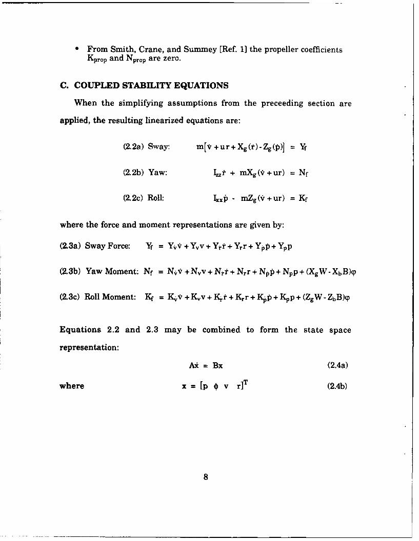
C. COUPLED STABILITY EQUATIONS
When the simplifying assumptions from the preceeding section are
applied, the resulting linearized equations are:
(2.2a) Sway: m[,+ur+Xg(r)-Zg(p)] = Yf
(2.2b) Yaw: Izr + mXg(v+ur) = Nf
(2.2c) Roll: Ixxp - mZg(,v +ur) = Kf
where the force and moment representations are given by:
(23a) Sway Force: Yf = YvV + Yvv + Yrt + Yrr + YpP + Ypp
(2.3b) Yaw Moment: Nf = N.v +Nvv+Nrt+ Nrr+Npp+Npp+ (XgW-XbB)(P
(2.3c) Roll Moment: Kf = K-v + Kvv + Ktr + Krr + Kpp + Kpp + (ZgW -ZbB)4p
Equations 2.2 and 2.3 may be combined to form the state space
representation:
Al = Bx (2.4a)
where x = [p 0 v r]T (2.4b)
8
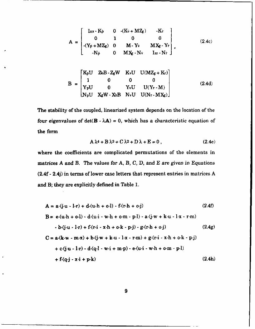
[ Ixx-KP 0 - Kv+MZg) -Kr
A= -(Y +M Zg) 0 M- Yv MXg-Yr
-Np 0 Mg -Nv Iz,-Nt
[KPU ZbB -ZgW KvU U(MZg + Kr)
B= 1 0 0 0 (.d
KYPU 0 YvU U(Yr -M)] 2dNpU XgW0- XbB NVU
The stability of the coupled, linearized system depends on the location of the
four eigenvalues of det(B - UA) = 0, which has a characteristic equation of
the form
A X4 + B;L3 + CX2 + D X + E = 0, (2.4e)
where the coefficients are complicated permutations of the elements in
matrices A and B. The values for A, B, C, D, and E are given in Equations
(2.4f - 2.4j) in terms of lower case letters that represent entries in matrices A
and B; they are explicitly defined in Table 1.
A - a.(j.u - Ir) + d.(u.h + o.1) - f.(rrh + o-j) (2.4f)
B-- e.(u.h + o-l) - d.(u.i - w-h + o-m - p.1) - a.(j.w + k-u - 1.x - r-m)
- b.(j.u - I1r) + f.(r.i - x.h + o.k - p-j) - g.(r.h + o.j) (2.4g)
C = a.(k.w - m.x) + b.(j.w + k.u - l.x - r.m) + g.(r.i - x-h + o.k - p-j)
+ c.(j.u - l-r) - d.(q.l - w-i + mrp) - e.(u.i - w.h + o-m - p.1)
+ f.(q.j - x.i + p.k) (2.4h)
9

D = g.(q.j - x-i + p-k) - f.q.k + d.q.m - e.(q.1 - w.i + m.p) - b.(k.w - m.x)
- c.j.w + k.u - l.x - r-m) (2.4i)
E = c.(k.w - m.x) + e.q.m - g.q.k (2.4j)
TABLE 1. COEFFICIENT DESCRIPTOR VALUES
a = Ixx-Kp b = KpU c = ZgW-ZbB d = MZg+ Kv
e = KvU f= Kr g = MZgU h = MZg + Yp
i = YpU j =M-Yv k = YvU I = MXg-Yr
m = U(Yr-M) o Np p = NpU q =XbB-XgW
r = MXg-Nv u =Izz-Nr w = U(Nr-MXg) x NvU
D. UNCOUPLED STABILITY EQUATIONS
Using matrices A and B from the preceeding section (Equations 2.4c and
2.4d), uncoupling the steering and roll equations is straightforward:
STEERING EQUATIONSM-Y, MXg-Y YvU U(Yr-M) I[v(
MMXg-N- Iz-N "I [I= LNvU U(Nr-MXg)J (2.5a)
ROLL EQUATIONS
0 1] 1 []J M(2.5b)
10
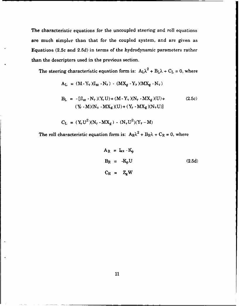
The characteristic equations for the uncoupled steering and roll equations
are much simpler than that for the coupled system, and are given as
Equations (2.5c and 2.5d) in terms of the hydrodynamic parameters rather
than the descriptors used in the previous section.
The steering characteristic equation form is: ALX.2 + BLX + CL = 0, where
AL = (M- Yv )(Izz - Nr ) - (MXg - Yr )(MXg -Nv )
BL = [Izz -Nr )(Yv U) + (M -Yv )(Nr - MXg )(U) + (2. 5c)
(Yr -M)(N, - MXg )(U) + (Yr -MXg )(NvU)]
CL = (YVU 2)(Nr -MXg) - (NvU 2)(Yr-M)
The roll characteristic equation form is: ARX2 + BRX + CR = 0, where
AR = Ixx-KP
BR = -KpU (2.5d)
CR= zgw
11
III. RESULTS AND DISCUSSION
A. DEGREE OF STABILITY
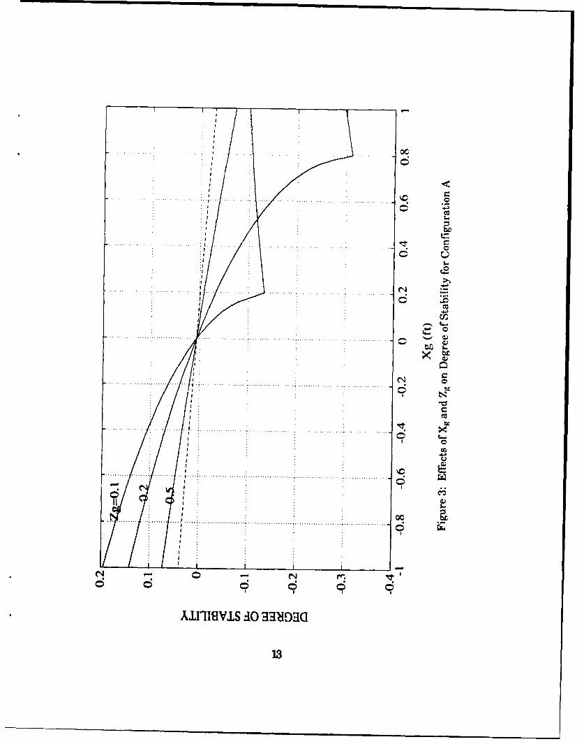
The effects of changing the longitudinal and vertical centers of gravity
(while keeping the center of buoyancy fixed at the vehicle center) on the
degree of stability for configuration 'A' is illustrated in Figure 3. Degree of
stability as utilized in this thesis is defined as the maximum real value of all
characteristic roots, with negative values indicating a stable situation. The
degree of stability for the uncoupled system is represented by the dashed line.
It can be seen that the critical value of Xg for which motions become unstable
is clearly a function of the metacentric height Zg, whereas the uncoupled
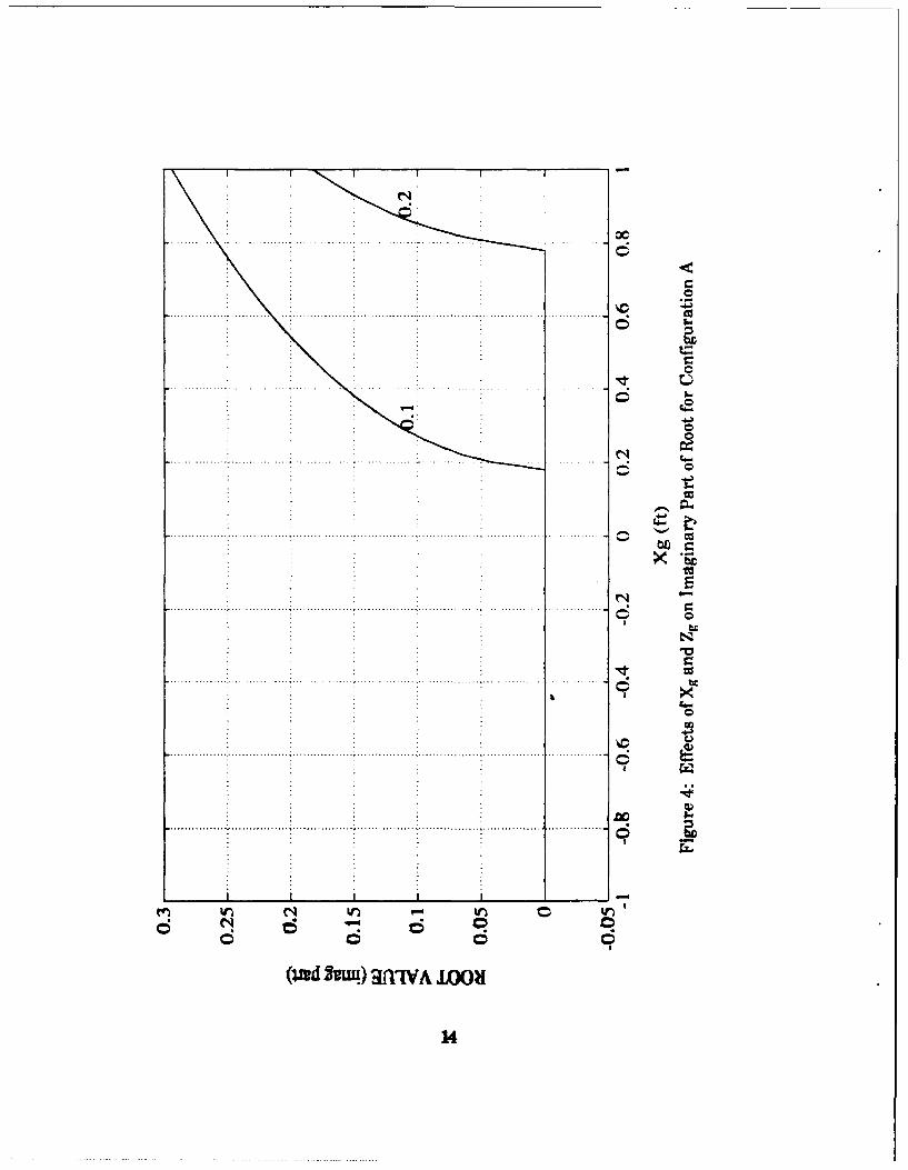
system predicts a constant value of Xg. Figure 4 displays the variation of the
imaginary part of the root value for configuration 'A'.
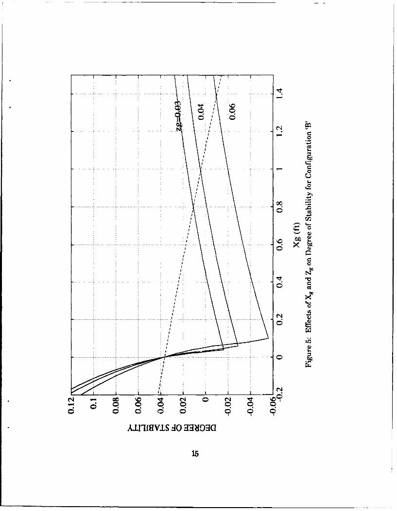
Figures 5 and 6 are analogous to Figures 3 and 4 for configuration 'B';
they show the degree of stability for varying Xg and Zg values. For this
configuration, the degree of stability has a stronger dependence on the
location of Xg and the value of Zg. For almost all positive values of Xg, the
complex conjugate roots are increasing in value and eventually becoming
positive; this indicates an oscillatory response that diverges when the degree
of stability is positive.
B. REGIONS OF STABILITY
Figure 7 shows the region of stability for configuration 'A', with the
uncoupled system represented by a dashed line. The uncoupled system
predicts stability for all values of Xg greater than 0.18 ft, while the coupled
system predicts an additional region enclosed by the triangular area to the
12
o-
C Q
000........... .............. ....
eq6C5 C5 C
AJLIIGVIS doMOU
130
Dc
............................................. ... .. ...... 6105
.. ...........
. . .. . . . . . ....... .... ...
............... ~ 0.. ..... ... .. ...... ....... .. ...... ..... .. .. . ..
C5 g
en W6N t n c W
(Wd 2uu) 3WA IM
14b
.~~~. .. . . .
C5
.... .... .... .... . -I.w
0 fu
0 0
IIISI I. MO
15*
I I
a 0
.* ........... (N
C)
(urdWrwi 3flIVA 001
166
0r
00 C4
0j) 20
17N

left of the dashed line. Figure 8 is analogous to Figure 7 for configuration 'B'.
The large discrepancies between the predicted regions of stability in this case
occur for Zg values less than 0.045 ft. For small values of Zg, there are
corresponding small regions of Xg where stability is predicted by the coupled
equations but not by the uncoupled equations. The root values in this region
are complex conjugates with very small real parts. Figures 9(a) and 9(b)
illustrate the effect of co-locating Xb and Xg. This results in a degree of
stability for the coupled system that is nearly identical to the uncoupled
system.
C. INTERPRETATION OF RESULTS
It may be shown by applying Routh's criterion [Ref. 4: pp. 211-218] that
for a fourth order equation of the form AX4 + BX3 + CX2 + DX + E to have
roots with all negative real parts the following must apply:
i.) BCD- AD2- EB2 > 0
ii.) E > 0.
If the quantity TE' is less than zero, the system will become unstable and the
resulting motion will be a simple divergence. If, however, the value of the
quantity BCD - AD2 - EB2 is negative, the resulting instability will result in
an oscillatory motion due to the presence of complex conjugate roots with
positive real parts.
For the coupled system of equations, the condition E = 0 yields:
Zg = Xg "[Ky(YrM)/(YvNr - Nv(YrM))].
while the uncoupled system of equations reduces to a constant term
expression for Xg:
Xg = [(MYv)/(YvNr - Nv(YrM))].
18

0
m m
000
..... .... ..... .. .... ....
006o
ci•
(U) wz
19

/ +
oco
.~ ~ ~~~, ... .....
X£IqIl~mS O 3g•CIDC
m/
/5
C;C
ot
00.... .... .. .............. ......................... ..... ......
* C 9 C5
el -~vs.0 -3O
* 0 0 0 2D
............. ....ti
. . .. .. . . . ... ..... . ...... .. .....
... .. .. . ... . .. ... .. ... ..... . 0
. ~~ . . . . . .. . .. . .. . . . . . . . . . .........
0L a
00
4.5 66 66
AJITIVIS O MO
I2
This explains the differences in the regions of stability illustrated in Figure 7,
since the above equations show a linear relationship between Zg and Xg for
the coupled equations and a constant value for Xg for the uncoupled
equations. When the value for Xg coincides with the value for Xb, the
constant term 'E' in the coupled equations is reduced to that of the constant
associated with the uncoupled equations, and the resulting predicted degree
of stability no longer depends on the value of Zg. Substituting the coefficient
values for 'E' serves to clearly illustrate the reduction:
E = (ZgW)[(YvU2XNr-MXg) - (NYU2)(YrM)] +
(KvU )(Yr-MXXbB-XgW) - (MZgU)(YvUXXbB-XgW).
When Xb = Xg and B = W for the neutrally buoyant case, the second and third
terms are reduced to zero. When 'E' is then set equal to zero (the condition
for determining where the real roots change from negative to positive), the
dependence on the value Zg is removed and the expression for Xg is the
constant given for the uncoupled equations. This reduction is the explanation
for the appearance of Figures 9(a) and 9(b). When the longitudinal centers of
buoyancy and gravity coincide for a neutrally buoyant vehicle, the degree of
stability for the coupled system of equations covering all metacentric height
values is equivalent to the uncoupled system of equations.
A simple reduction of the equation resulting from Routh's criterion to
determine when a pair of complex conjugate roots crosses the zero axis is not
easily accomplished. Figure 10 is presented as confirmation that the
locations of Xg for which BCD - AD2 - EB2 = 0 matches the locations given
graphically in Figure 5.
22

.. . .. .. . . . . . . . .. .I
I-
. . .. ... ... .
Nc
C 561C.
6 O0
. . ... ... . ... . ... .. . .... ..
00 e0
Io
fzv~v)-3zv)-(C-M)uazvmN
236
D. LINEAR SIMULATIONS
Figures 11 through 14 present comparisons of the coupled and uncoupled
system responses for configuration 'A'. For the stable cases Xg = 0.40 ft and
for the unstable cases Xg = -0.20 ft, while Zg is 0.20 ft for both. The unstable
coupled case (Figure 11) illustrates a simple divergence for both angle of drift
and roll angle. This is expected since the roots are not complex conjugates.
The unstable, uncoupled case accurately predicts the divergence in angle of
drift, but the roll response is predicted to be stable. This may be explained by
examining the uncoupled equation of motion in roll:
04" - 0' (KpU)/(Ixx -Kp ) + 0 (ZgW)/(Ixx - Kp )=0.
Substituting values for configuration 'A' yields:
4" + 0' (1.475) + 4 (0.720) = 0.
The solution of this equation results in a natural frequency of 0.85 rad/sec
and a damping factor of 0.869. This is an underdamped case, since both roots
have negative real parts and are complex conjugates. Substituting values for
configuration 'B' yields:
4" + 0' (1.475) + 4 (0.144) = 0.
The solution for this case results in a natural frequency of 0.380 rad/sec and a
damping factor of 1.941, which represents an overdamped situation. This
also demonstrates that a vehicle's natural frequency in roll may be increased
by increasing the metacentric height. The effects of the underdamping may
be seen in Figures 12 through 14.
Figures 15 through 20 provide a comparison between the coupled and
uncoupled equations for configuration 'B'. The effects of the overdamping are
evident in figures 15 through 17. This set of figures demonstrate the
24
C
....... ~ ..-...... . .... .. ......... N....II
/ . r
... .... . ..... . . . . .. .
: .I-.I
I .1
.... . . . . .. ....... .... . .. . .. . .. . . ..- .
jeen
I0
S.. .. . . .. . .....
'2-o ,•U ¢al
N .-
a a a I I
CN
oc W
.. ... .... .. , "
..............
c
. . . . ..... . ... ... .. .. . . .. . .. . . .. . . . .. .. . . . . . .. . . . .. .. . . . . o . .. . . .. .. . . . . . . .. . .... .. .. . . . ....0 . .
. iI N
I -
- I
.. ................. .................... ;...... .. ................ .. ... .. .. . 0
-- -- ----
i i ... •... .. .. -• -
6 C5
26
a CA
....... .....
St 0"
II U
• •,,
.. ............................. ............ ........... ....... . ..... ..... .............. • ...: ..... ....... ....
0 0
................................................ .................. ............ 4 ..... ... ............... -........c,,"1
).
27
I 0
I. C

I w
.. .. .. .. .. . . . . . . . . . . .. .. . . . . . . .. . . . .
* . I
... ... ... ... .. ... ... ... ... t.. . . . . . . .. . . . . . . .
I4- w t
*1w*1m
0. .. ................. . ....
.-.. ..... .0... ... .. ... .. ... .. .. ..... .. .. .. .... .. .. ... .. ..
........ ...... * .. .............. .. .. .. ................
280
I II "'
* /
S: i /
......................
S.. ......... : ,............ .... ........... ....... .............. . ............. .. ..... ...... ... ... . . . . .-. 8 .
m tx
-II
........................... ...... • .. ........ .. : ........ ..... , xkN
.... .. .. . .. ... .... ... .. ... ... .. . . . .. ... .. ... .. . . . .. .. .. ........ .... .. ... ... - . . . . . .. . ... . . .... . .. ... ....
: : 0
In.i; -~
= •m. • Hi II II i II II I
I- bLg
290

....... . . :. ...........' : . . . . . . . .... ............... ................. ......... ....... : . . . ., .....
. . . . .. I
I> 0.... ... ... .. ... ... .. ........ .. . .. .. .. ... .! . .... . ..... .. I ....... .. .. • .... ... .. . ...: , " f
o,
... ............. ....... ........ ].... ........... ... :.. ............ .... .... ......... .......... ... .- . ...... .. .. 0¢
300
I•• / 0
: : : : : r '
S ........ ...,.9
SI I
S33?1O03
30
. ............. . .-. . ... ......... .. . ... .... . .... ...... .' . . . . . . ... . . .........
co
I$.
trIt
* I p
S.. ........• .................. • .......... . . { . . . . .... ............. ........... ., . ............ .
smogu
3 I1
31I
cz.
............. cr2
0 4t
t/ .- uI.. .. . . . . . . . .. .
* 66
--------------------
I
-noa
I-*2~
- -
---------- ------ -- - - -
- -- --- -- --- - - -
-------- ----- ----
00
-j-
00. N 0
.. . . . . .. .. ... .. .. .... ...
----- ----- -----
bi)
.. . .. .. . . . . . . . .. . . . . .. . . . .. . .. . .
bC
- a)
.. ... ... ............. ..... ...... .. ....... ... ... ...
III I
S.. .. . ............. .... ... ... ............. i .......... . .......... ....................... : ........ . . . . . . ¢
ao IV q0 3
34
magnitude of the discrepancies when the coupling effects are not considered.
The comparison below summarizes the results of the figures representing
simulations for configuration 'B', where 'C' stands for coupled and 'UC' for
uncoupled.
uc C UC C UC
Xg 0.20 0.20 1.00 1.00 1.50 1.50
Roll Stable Y Y N Y N Y
Drift Stable Y N N N N Y
As was seen before, the effects of the coupling on the system results in
complex conjugate eigenvalues with positive real parts. Therefore, the larger
values of Xg result in increasingly divergent oscillations instead of the
stability predicted by the uncoupled system.
Figure 21 is a three-dimensional presentation of the roll amplitude vs
time for configuration 'B' as Xg varies from 0.15 ft to 1.50 ft. This mesh
capability of MATLAB allows a comparative view of several solutions, and
the behavior of the roll response for the coupled system is easier to discern.
E. NON-LINEAR SIMULATIONS
In order to provide a measure of the accuracy of the results obtained
utilizing the linearized equations of motion, a simulation program for the
non-linear equations of motion was developed using Hamming's method
[Ref. 2]. Hamming's method utilizes a Milne predictor and incorporates a
modifier step prior to the correction step. The primary advantage of using
Hamming's method is that only two derivative function evaluations are
35

0
0)
required per step rather than the four or more normally required by other
popular methods. The local error is of the same order of magnitude (h4) as a
more time consuming process such as a fourth order Runge-Kutta, but the
reduction in function evaluations results in a faster simulation. The formula
is presented below, and may also be found in the nonlinear computer
program simulation in Appendix A.
HAMMING'S METHOD
Y(i+l)predicted = y(i-3) + (4h/3)[2f(i) - fMi-1) + 2f(i-2)]
Y(i+l)modified = Y(i+l)predicted - (112/121)[Y(i)predicted - Y(i)core"ctd]
Y(i+l)corrected = (1/8)[9y(i) - y(i-2) + 3h(f(i+l)modijfied + 2f(i) - f(i-1))]
y(i+1) = Y(i+l)corrected + (9/121)[y(i+1)predicted - Y(i+l)corrected]
The first four values must be determined by another method; the Euler
linear solution with a small step size 'h' proved sufficient.
Figure 22 represents the simulation for the unstable representation of
configuration 'A'. Rather than the exponentially increasing roll angle and the
-90 angle of drift computed with the linear simulation, the nonlinear solution
predicts an angle of drift that reaches -15 degrees, and then slowly diverges.
The roll angle reaches a steady state value of approximately three degrees.
Figures 23 and 24 are the nonlinear simulation results for stable
configurations of 'A' and 'B', respectively. They are nearly identical to the
results obtained using the linear simulation and displayed as Figures 12 and
18.
Figure 25 is the simulation for an unstable configuration 'B'. Quite
notable are the steady state roll angle and angle of drift after approximately
250 seconds rather than the exponentially increasing divergence apparent in
37
. 9cz
> C
S.. . . . . .... . .. .. . .. .. . .. .. .. . .. .. . .. .. . . . . . . . . . . . . . . .. . . . . . . . . . .
C4"9
4i - g .u
3I
-, 0- i
* ., rT II
- 0
iI
II
S.............. ....... .... ...... ............... ...,. . . . . . . . . . . ....... •
9 5.
(sooiop) 31DNV
318
0 -+
0 ,"-
CN
0-sS......... ......... ........ .......................... .... ."....,.,S.. . . .. .. . .. .. . .... .. . .. .. . .. .. . .. . . . . .. .. . .. . . . .. ... . .. . .. .. . .. .. . .. .. . .• . .. . . . . . . . . . . . . . . "
i~~c i •,
S.. ..........: .... ........ ............ .. ... .. .............. ! ........, ... .. . • ............ .. •
.. . ...... . .... ... ....... .. .. ...I ......
. . .... . ..... :.. ............ ...... ".. ......... .. ..... . . . / ... ... ........ .......-" •. .. ..... . . "
I..
I.
00 N
(SoajB;0) gCi..V
39<
0
........................ ....................... i . . . .. ........ ..... r " z 2........... • .....................
400II
(s•B~p) -DI
-- --- - --- -0
---------------- -----------------
- - - -- - - -- - -- -- -- ------- - - - - - - - - - - - -
- ---- - - -- - - - - - -- - - - - - - - - - - -
------ -----------
-----------------------
-- -- --- - ----- --------- ----
----------
---- ----
- - - - - - -- - --a- - - -
---------------- U
----- I--------------
*------ ----- --
- -- - - -
---------- -------
............ ...
- -- - - --- j-- -
-- ---- ---
------- if
-------------
Iz C
41-- --- C

00- II
-o
.. . . . ...................... ................. ... ...... ............. -............ ....... . .. . .. . • '
.. . .. ... .....
-EN
... ...... .. ............... ... .............. -. / ........... ... ;...... ......... .... .... .. ....... .. <
. . . . . .
4.2
C1
.4 . .. . . . .. . . .. .O
...... ... ........... ..... ...
.- sM
........... ~~~ ~ ~ ~ ............... ..... ...... 0...... cr
aI.. . .... ... ..
........ .... . ...... .....
......... .. . . . . . . . . . . . ... . . . . . . . . . . . ... .. .. .. .
* . . I
*Soip . . -
* . .43

0x
. . . .. . . . . . .. ... . . .. . .. . . .. . .. . . . . . .
.............. .............. .......... .. ...........- ....Qt
r.
.... .. .............. ..... .... .... ......... . ... ......... ..........
2<
E--
oc
0
............................. .............
4jI
(scow2ap) jimwj aa 3-1NV c
44

the corresponding linear simulation. Figure 26 provides a comparison
between the linear and nonlinear solution for angle of roll. The enlarged
view of the steady state region provided in Figure 27 better illustrates the
constant limits of oscillation. By plotting the roll angle versus the angle of
drift, an elliptical trajectory is apparent in Figure 28. This result is similar
to the results obtained by Schmidt and Wright in their analysis of high
performance aircraft wing-rock [Ref. 5]. They postulate that a possible
explanation for the limit cycle is the inertial coupling between a stable
longitudinal and an unstable lateral mode. Similar results in tho work are
attributed to dynamic as well as hydrodynamic coupling. Figures 25 and 28
indicate that the nonlinear interactions for the unstable conditions of
configuration 'B' provide a significant amount of damping to the rolling
motion. The limiting of the rolling motion accomplished by including the
nonlinear terms then serves to limit the buildup of the angle of drift and the
result is an eventual stable limit cycle.
The ocean environment can be expected to introduce many combinations
of disturbance forces, which may or may not be periodic A preferred method
for simulating many disturbances such as sensor noise, ocean current
fluctuation, and vehicle acceleration fluctuations is to model thcm as 'white
noise'. Figure 29 is presented to demonstrate the effects of including
constant, zero-mean disturbances in sway and yaw on the marginally stable
system of configuration 'B'. The disturbances are developed using MATLAB's
random number generJtor with a uniform di.tribution. ('he rnndom numbers
are then scaled to simulate values that may be _ Lpected. The variance of the
sway and yaw acceleration disturbances, resoectively, for Figure 29 are 0.003
(ft/s 2)2 and 0.002 (rad/s2 )2 . The resulting simulation bears little resemblance
45

to Figure 24, although the initial conditions and values for Xg and Zg are the
same. With even these relatively minor disturbances acting on the system of
configuration 'B', a rather large, non-symmetric oscillation in both roll and
angle of drift is evident. Although the system is still stable, with the mean of
both the roll angle and angle of drift equalling zero, a limit cycle similar to
that of the unstable configuration (Figure 25) has developed. As the angle of
drift fluctuates between positive three degrees and negative four degrees, the
angle of roll varies between positive and negative two degrees. Increasing
the scaling (which increases the variance) for the disturbances would be
expected to increase the fluctuations until stability is lost. Similarly, it is
true that the small disturbances acting in Figure 29 have a greatly reduced
effect on the system of configuration 'A', which has greater stability.
46

.- 3
1-4t
U0,
E-4
ql N 0 m I'* te
(s22ig;p) WaioNV
47

IV. PERTURBATION ANALYSIS
A. BACKGROUND
The previous section demonstrates that knowledge of the separation
between longitudinal centers of buoyancy and gravity is critical in
determining system stability. If this quantity is the dominant factor in a
stability analysis, then an approximation for the degree of stability may be
developed by applying perturbation theory. Although perturbation results
are only approximations, their advantage over numerical methods is in
illustrating the degree to which a solution depends on the variable(s)
involved. From the fundamental theorem of perturbation theory [Ref. 61, we
seek a solution to the characteristic equation AX4 + BX3 + CX2 + DX + E = 0 of
the form:
n =-
X(E) I an.iE n(4.1)n=O
where E is the variable of interest and the solution approximates the
numerical solution in the region where E is small. The constant coefficients
(ao, al, ..., an) are all independent of E, and are afllequal to zero for small c.
B. PERTURRATION FORMULATION
Recalling Equations 2.4f - 2.4j, which daehied the coefficients of the
quartic characteristic equation, it would obviousb, be desirable to simplify the
equations as much as possible prior to formulating the perturbation
48
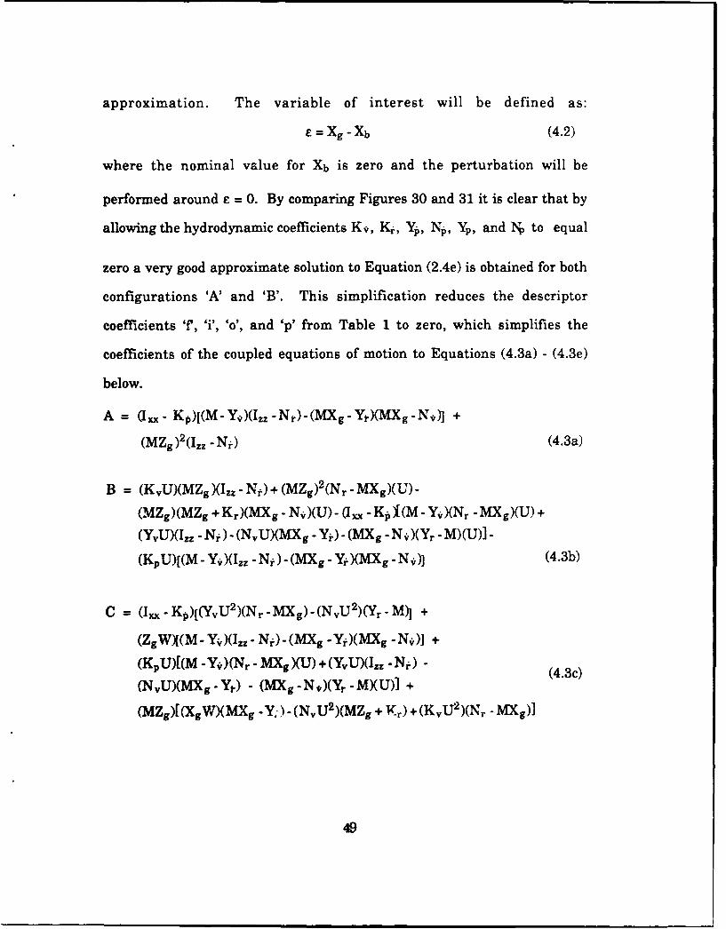
approximation. The variable of interest will be defined as:
£ = Xg - Xb (4.2)
where the nominal value for Xb is zero and the perturbation will be
performed around £ = 0. By comparing Figures 30 and 31 it is clear that by
allowing the hydrodynamic coefficients K*, Kr, Yp, Np, Yp, and IS to equal
zero a very good approximate solution to Equation (2.4e) is obtained for both
configurations 'A' and 'B'. This simplification reduces the descriptor
coefficients 'f', 'i', 'o', and 'p' from Table 1 to zero, which simplifies the
coefficients of the coupled equations of motion to Equations (4.3a) - (4.3e)
below.
A f (Ixx- Kp)[(M-Y4 )(Izz-N )-(MXg-Yt)(MXg-N4)I +
(MZg) 2 (Izz -Nj) (4.3a)
B = (KvU)(MZg)(Izz - Nt) + (MZg) 2(Nr - MXg)(U)-
(MZg)(MZg + Kr)(MXg - Nv)(U) - (I xx - Kp )I(M - Yv)(Nr -MXg)(U) +
(YU)(Izz -Nj) - (NvU)(MXg - Yj) -(MXg -N v)(Yr - M)(U)] -
(KpU)[(M - Y-)(Izz -Nr) - (MXg - Yi)(MXg -N -)] (4.3b)
C = (Ixx- Kp)[(yvU 2 )(Nr-MXg)-(NvU 2)(Yr" M +
(ZgWX(M- Y)(Izz -N) -(MXg- Y)(MXg- N•)I +
(KpU)[(M -Yj)(Nr - MXg)(U) + (YvU)(Izz - Nj) - (4.3c)
(NvUXMXg-Yt.) - (MXg-Nv)(Yr-MXU)l +
(MZg)[ (XgW)(MXg - Y,') - (NvU 2 )(MZg + Y-r) + (KvU 2 )(Nr" MXg)1
49
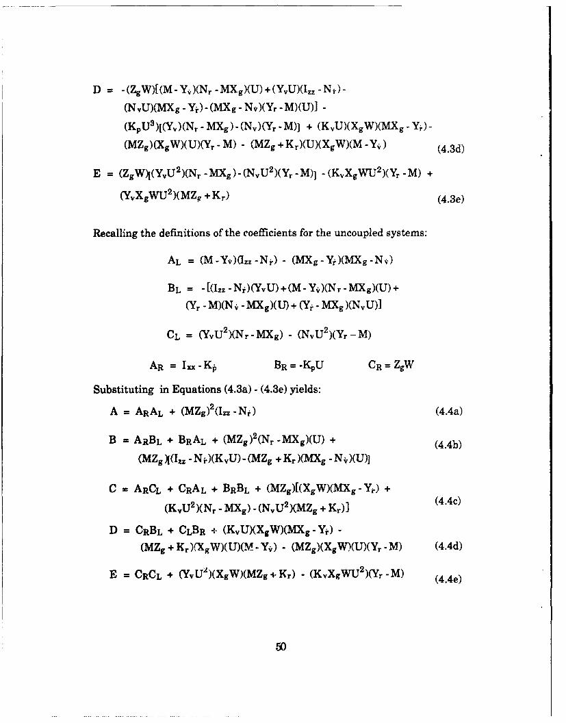
D =- (ZgW)[(M - Yv)(N - MXg)(U) +(Y-,U)(I 2 - Nr) -
(NvU)(MXg- Yr) -(MXg -Nv)(Yr -M)(U)] -
(KPU 3 )[(Yv)(Nr -MXg) -(Nv)(Yr -M)] + (KvU)(XgW)(MXg - Y0-
(MZg)(XgW)(U)(Yr - M) - (MZg +Kr)(U)(XgW)(M -YO) (4.3d)
E=(Z9W (vU)(Nr -MXg) -(NvU 2 (r~ - (K, WU)(r -M) +
(YyXgWU 2 )(MZL- +Kr) (4 .3e)
Recalling the definitions of the coefficients for the uncoupled systems:
AL = (M-Yv)(Izz-Nk) - (MXg-Yi)(MXg-Nv)
BL = - [(Izz-Nr)(YvU) +(M -Yvý)(Nr -Mag)(U) +
(Yr -M)(N ý MXg)(T) + (Yj MXg)(N, U)]
CL = (yvU2 )(Nr-MXg) -(NvU 2 )(Yr -M)
AR =Ix, KP BR -KpU CR =ZgW
Substituting in Equations (4.3a) - (4.3e) yields:
A = ARAL + (MZg)2z (~- Ni) (4.4a)
B = ARBL + BRAL + (MZg) 2 (Nr -MXg)(U) + (4.4b)
(MZg )I(Izz - N j)(K vU) - (MZg + Kr )(MXg - N -)(U)I
C = ARCL + CRAL + BRBL + (MZg)[(XgW)(MXg - Yr) +
(K vU2 )(Nr - MIXg) -(Nv U 2)(MZg + Kr)] (4.4c)
D = CRBL + CLBR + (KvU)(XgW)(Ixg -Yi) -
(MZg +Kr )(XgW)(U)(M - Y- - (MZg)(XgW)(U)(Yr -M) (4.4d)
E = CRCL + (YvU 2)(XgW)(MZg +Kr) - (KvXgWU-T2 )(Yr -M) (.e
50

a-N. I . .
000
S.. ..• ' " ... .. • ... .. ..• . ..- ....... •.... . : .. . ............ i " . '
bk... .. . ..... ...
~~~- .... ..... .......... ..! ... . .. ....a .. ......... .. . . .
......i...... ... •.. ....... i ... .• . ...... .... ..i .... ... ............. : . . . .
S.. .... ..i .. .. ... .I . . .. ....: . ....... i. .... .... ..... ... .. . . . ....... i . . . . . . .. . .. i. . . . . ".
S.. . . .".......... I ........... i.. ........... :............ " .......... '.... ........ ............ :. .. ......... ; .......... • " .
rr
0n 0- 0r ) 0 9 0l 0n V
I I I I
AlIH r•f.V.S .,O .33ITOEIG
. . . .. . ... . . . . . . . . . . . . . . .. .
.. . . . . . . .. .. . . . .. .. . . . . .I
.. .. .. .
0c
N tic
Eg. . . . . .... . . . . . ...... .....
* 'o
....... ....~~ .. . . . . . . . . . . . . .
OCz
Iin
....... ......... ........
00 ND0
52
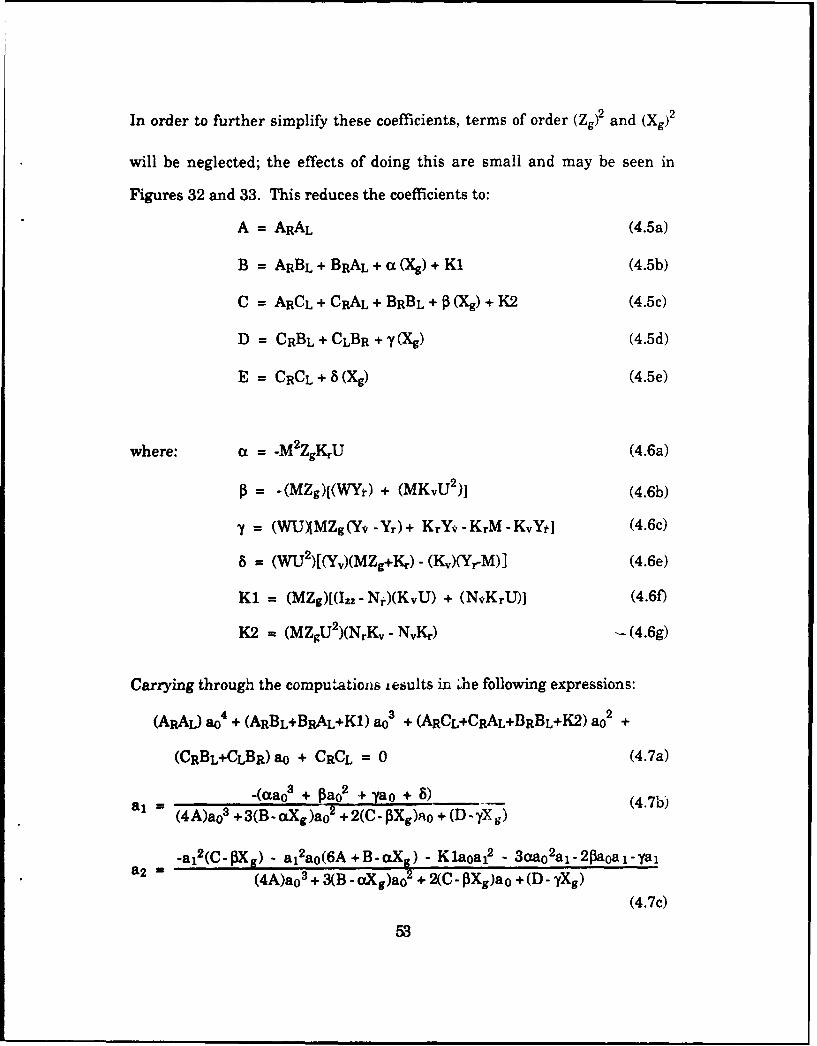
In order to further simplify these coefficients, terms of order (Zg) and (Xg)2
will be neglected; the effects of doing this are small and may be seen in
Figures 32 and 33. This reduces the coefficients to:
A = ARAL (4.5a)
B = ARBL + BRAL + a (Xg) + K1 (4.5b)
C = ARCL + CRAL + BRBL + P (Xg) + K2 (4.5c)
D = CRBL + CLBR + If(Xg) (4.5d)
E = CRCL + 8 (Xg) (4.5e)
where: a = -M2ZgKrU (4.6a)
P = - (MZg)[(WYt) + (MKvU2)] (4.6b)
,y = (WUXMZg (Yv -Yr) + KrYv -KrM -KvYrI (4.6c)
8 = (WU2)[(Yv)(MZg+Kr) - (Kv)(YrM)] (4.6e)
K1 = (MZg)[(Izz - Nj)(KvU) + (N*KrU)] (4.6f)
K2 = (MZgU 2)(NrKv - NvKr) -- (4.6g)
Carrying through the computations iesults in ýhe following expressions:
(ARAL) ao4 + (ARBL+BRAL+K1) a03 + (ARCL+CRAL+BRBL+K2) ao2 +
(CRBL+CLBR) ao + CRCL = 0 (4.7a)
-(aaoe + Pao2 + yao + )(4.7b)a1 = (4A)ao3 +3(B-aXg)ao2 +2(C-j3Xg)ao +(DI- 7X g)
-al 2 (C-Ag) - a12ao(6A+B-ozXI) - Klaoal2 - 3aao2aj-2lPaoal-yaja2 (4A)ao3 + 3(B - aXg)ao2 + 2(C- OXg)ao + (D - yXg)
(4.7c)
53
a oc
....... ..... ..... ........ .............
66
54.
!I I I I
.. . .. .. .. ... ;. .. ... .. .. ... :. . . . . .;.. . .. .. .. .. i.. .. .. . .:.. . .. ....... . .. ... .. . .. .. ... .. . .. ... . .. .. I
i.i
* (N
>
-
I.N
I I
0 0
JUITVIS o MO
55N

The characteristic equation AX4 + BX3 + CX2 + DM + E = 0 may now be
expressed in terms of a second order perturbation which depends on a single
variable e as:
X(c) = ao + al, + a2 E2 (4.8)
Figures 34 through 37 depict the results for both first and second order
perturbation analysis about Xg close to zero. Results for both configurations
'A' and 'B' demonstrate that this method for representing the degree of
stability in the vicinity of a nominal (Xg - Xb) is quite satisfactory, provided
the roots have no complex conjugates. In the region where the roots become
complex, the problem is no longer a regular perturbation, and methods to
solve the singular perturbation must be developed.
56
I I I 6
* . // 0I
I,5
.. ....... .... ..... . . .. .. ....... : .. ..... ... ... .. .. i . . ... . ..... . ' ... ... ... .. ..... .. ..... .......
... ........... ....- .............. . ........ ............. ..... ... . -.. .......... ........
.......... .. .. .. .. .. .. .. .. .... . .. . . . . . . . . . . . . ... . . . . . . . . . . . . . . . .. . . . . . . . .. . . . . . .. . . . .
/ 0
6 •...~~ ~ ~ ~ ... . .. . . . . . . .
/ IIt
* C 0
1 1
lnqI: aoMO
570
.. . . . . .. . . .. . . .. . . .
I..
SI.
-/ -
co
S. .. .......... ........ !..... .... ............. ....... .. ......... / .... ...... ....... ...... ...... .. .. ...... •=
a C
r-
...............~~........ i . ......... .... ........ ... ... ... ..... .... ......, .. ......... .......... =
6g
/ Q
C-
. .. ... .. ... ...... ..... ......... ... . . . ..... .... ¢ "
Si.0
C56.uri i , MOM 0
580
II. 6
£•L~I•€$ =IO.q3•OI-
* 68
III I * "
- 6/
. ... .
.. .. .. ..
6 ,.
I,.* I$ 0
* . * I
S. IIIL Jo MOM
II. I . I-
* ,I 0* * III& O•"D
NI-
/
6- 0
S * -
S .-I *
0
Q
- . 0
*1 - 0 0'S 6
0I-
�,-S
0
I-
0*0
* I * -�
0-
6* I I 0
6
0 6- 6 0 0 66 6 6 I 6
AIflIfiVIS dO H�193G

V. CONCLUSIONS AND RECOMMENDATIONS
"* When considering an inherently stable situation for an analysis of sway,
yaw, and roll response, the linear simulations compare favorably w i t h
the nonlinear simulations. For a marginally stable or unstable system,
only the nonlinear simulation can predict the existence and extent of any
non-zero steady states or limit cycles that may occur.
"* Obviously, in the design of a submersible, careful attention must be paid
to selection of both the metacentric height and the separation between the
longitudinal centers of gravity and buoyancy. Instability associated with
the dynamic coupling effects can be minimized by increasing the
metacentric height. The uncoupled system stability predictions are not
reliable when there is separation between Xg and Xb.
"* It can be concluded from the analysis that the coupling of roll into s w a y
and yaw for the linearized equations of motion is not very significant
when Xg equals Xb.
"* Recommendations for future modelling research include an expansion
to incorporate coupling effects between the vertical and horizontal planes.
It is well known that the coupling between translation and attitude is a
severe limitation in the design of submersibles.
"* The effects of varying hydrodynamic derivatives and initial conditions, as
well as incorporating disturbances in the nonlinear simulations deserve
more attention. Additionally, the complexity of the nonlinear system
resulting from including the vertical plane is greatly increased. More
studies of the nonlinear system resulting from this union are also
required.
61

APPENDIX A
NON-LINEAR SIMULATION PRO2GRAM:
"% THIS PROGRAM USES HAMM~ING'S METHOD TO SOLVE A SYSTEM"% OF NONLINEAR EQUATIONS. SIMILAR TO A FOURTH ORDER"% RUNGE-KUTTA IN TERMS OF LOCAL ERROR, IT REQUIRES ONLY"% TWO FUNCTION CALCULATIONS PER STEP VICE FOUR.
function[v,phi] = nonlinsim-hamniing(UO ,Xg,Zg)
"% VEHICLE PARAMETERS FOLLOW
W = 12000.0; hxx = 1760.0; Iyy = 9450.0; Izz=10700.0; L =17.425;
RHO=1.94; G=32.2; M = WIG; BUOY = W; Zb=0.0; Xb =0.0;
ZZ = O.5*RHO*L A2;
"% SWAY HYDRODYNAMIC COEFFICIENTSYpdot = 1.270E-04*ZZ*L A2; Yrdot = 1.240E-03*ZZ*LA 2;Ypq = 4.125E-03*ZZ*L A2; Yqr = -6.510E-03*ZZ*L A2;Yvdot = -5.550E-02*ZZ*L; Yp = 3.055E-03*ZZ*L;Yvq = 2.360E-02*ZZ*L; Ywp = 2.350E-01*ZZ*L;Ywr = -1.880E-02*ZZ*L; Yv = -9.310E-02*ZZ;Yvw = 6.840E-02*ZZ;
"% NOMINAL VALUE FOR Yr = 2.970E-02*ZZ*L"% CONFIGURATION 'A': Yr = 3.500E-02*ZZ*L"% CONFIGURATION 'B': Yr = 5.940E-02*ZZ*L
CC = input('enter model configuration choice; either 1 for A or 2 for B')
if CC<2Yr = -3.500e-02*ZZ*L;
elseYr = -5.940e-02*ZZ*L;
end
"% ROLL HYDRODYNAMIC COEFFICIENTSKpdot = -1.01E-03*ZZ*L A3; Krdot = -3.37E-05*ZZ*L A3;K~pq = -6.93EM5*ZZ*L A3; Kqr = 1.68EM2*ZZ*L A3;
Kvdot = 1.27E-O4*ZZ*LA2; Kp = -1.10E-02*ZZ*L A2;
Kr = -8.41E-04*ZZ*L A2; Kvq = -5.115E-03*ZZ*L A2;Kwp = -1.27E-04*ZZ*L A2; Kwr = 1.39E-02*ZZ*L A2;Ky = 3.055E-03*ZZ*L; Kvw = -1.87E-01*ZZ*L;
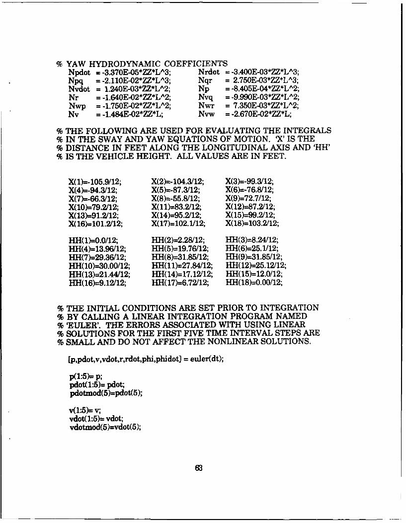
% YAW HYDRODYNAMIC COEFFICIENTSNpdot = -3.370E-05*ZZ*LA3; Nrdot = -3.400E-03*ZZ*LA3;Npq = -2.11OE-02*ZZ*LA3; Nqr = 2.750E-03*ZZ*LA3;Nvdot = 1.240E-03*ZZ*LA2; Np = -8.405E-04*ZZ*LA2;Nr = -1.640E-02*ZZ*LA2; Nvq = -9.990E-03*ZZ*LA2;Nwp = -1.750E-02*ZZ*LA2; Nwr = 7.350E-03*ZZ*LA2;Nv = -1.484E-02*ZZ*L; Nvw = -2.670E-02*ZZ*L;
% THE FOLLOWING ARE USED FOR EVALUATING THE INTEGRALS% IN THE SWAY AND YAW EQUATIONS OF MOTION. 'X' IS THE% DISTANCE IN FEET ALONG THE LONGITUDINAL AXIS AND 'HH'% IS THE VEHICLE HEIGHT. ALL VALUES ARE IN FEET.
X(1)=-105.9/12; X(2)=-104.3/12; X(3)=-99.3/12;X(4)=-94.3/12; X(5)=-87.3/12; X(6)=-76.8/12;X(7)=-66.3/12; X(8)=-55.8/12; X(9)=72.7/12;X(10)=79.2/12; X(11)=83.2/12; X(12)=-87.2(12;X(13)=91.2/12; X(14)=-95.2/12; X(15)=-99.2/12;X(16)=-101.2/12; X(17)=102.1/12; X(18)=103.2/12;
HH(1)=0.0/12; HH(2)=2.28/12; HH(3)=8.24112;HH(4)=-13.96/12; HH(5)=19.76/12; HH(6)=25.1/12;HH(7)=29.36/12; HH(8)=-31.85/12; HH(9)=-31.85/12;HH(10)=30.00/12; HH(11)=27.84112; HH(12)=-25.12/12;HH(13)=21.44/12; HH(14)=17.12/12; HH(15)=-12.0/12;HH(16)=9.12/12; HH(17)=-6.72/12; HH(18)=0.00/12;
% THE INITIAL CONDITIONS ARE SET PRIOR TO INTEGRATION% BY CALLING A LINEAR INTEGRATION PROGRAM NAMED% EULER'. THE ERRORS ASSOCIATED WITH USING LINEAR"% SOLUTIONS FOR THE FIRST FIVE TIME INTERVAL STEPS ARE"% SMALL AND DO NOT AFFECT THE NONLINEAR SOLUTIONS.
[p,pdot,v,vdot,r,rdot,phi,phidot] = euler(dt);
p(l:5 )= p;pdot(1:5)= pdot;pdotmod(5)=pdot(5);
v(1:5)= v;vdot(1:5)= vdot;vdotmod(5)=vdot(5);
63
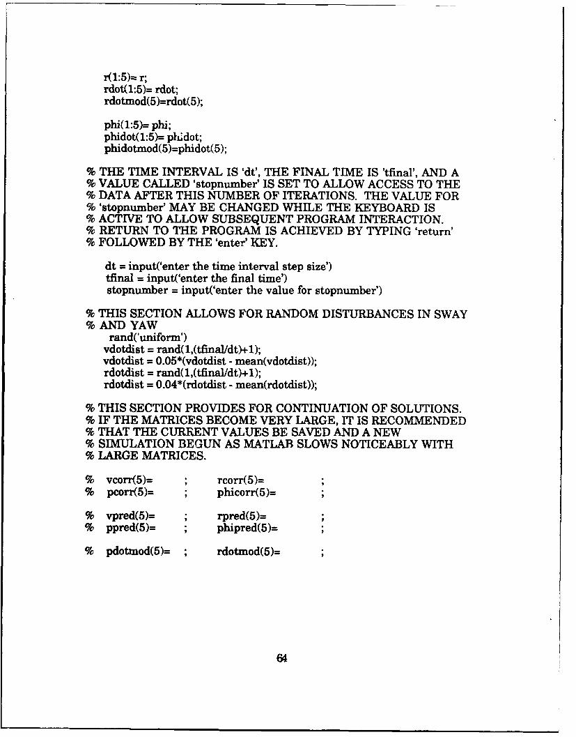
r(1:5)= r;rdot(l:5)= rdot;rdotmod(5)=rdot(5);
phi(1:5)= phi;phidot(1:5)= pbddot;phidotmod(5)=phidot(5);
"% THE TIME INTERVAL IS 'dt', THE FINAL TIME IS 'tfinal', AND A"% VALUE CALLED 'stopnumber' IS SET TO ALLOW ACCESS TO THE"% DATA AFTER THIS NUMBER OF ITERATIONS. THE VALUE FOR% 'stopnumber' MAY BE CHANGED WHILE THE KEYBOARD IS"% ACTIVE TO ALLOW SUBSEQUENT PROGRAM INTERACTION."% RETURN TO THE PROGRAM IS ACHIEVED BY TYPING 'return'"% FOLLOWED BY THE 'enter' KEY.
dt = input('enter the time interval step size')tfinal = input('enter the final time')stopnumber = input('enter the value for stopnumber')
"% THIS SECTION ALLOWS FOR RANDOM DISTURBANCES IN SWAY"% AND YAW
rand('uniform')vdotdist = rand(1,(tfinaI/dt)+1);vdotdist = 0.05*(vdotdist - mean(vdotdist));rdotdist = rand(1,(tfinal/dt)+1);rdotdist = 0.04*(rdotdist - mean(rdotdist));
"% THIS SECTION PROVIDES FOR CONTINUATION OF SOLUTIONS."% IF THE MATRICES BECOME VERY LARGE, IT IS RECOMMENDED"% THAT THE CURRENT VALUES BE SAVED AND A NEW"% SIMULATION BEGUN AS MATLAB SLOWS NOTICEABLY WITH"% LARGE MATRICES.
"% vcorr(5)= rcorr(5)="% pcorr(5)= ; phicorr(5)=
"% vpred(5)= ; rpred(5)="% ppred(5)= phipred(5)=
"% pdotmod(5)= ; rdotmod(5)=
64

% COMMENCE INTEGRATION
for i = 6:(tfinalIdt) + 1;
% THIS SECTION USES A HAMMING PREDICTOR-CORRECTOR TOOBTAIN VALUES
vpredQj)=voj-4)+(4*dt/3)*(2*vdotýj-1)-vdotQj*2)+2*-vdotoj-3));rpredQj)=r(j-4)+(4*dtI3)*(2*rdotoj-l)-rdotQj.2)+2*rdotoj-3));ppeo=ý4+4d/)(*dool-dt-)2poQ3)phipredj)=phiQj-4)+(4*dt/3)*(2*poj.1)-poj2)+2*pQj-3));
if j < 7vmodj) = vpredoj);rmodj) = rpred(.j);pmodQj)= ppred(j);pbimodQj)= phipredfj;
elsevmodO?)= vpred(I)-( 112/121 )*(vpredojj. 1)-vcorr(j- 1));rmodOj)= rpredoj)-(1 12/121)*(rpredoj-1)-rcorr(j- 1));pmodOj)= ppredoj)-( 112/121)*(ppredoj-l)-pcorrj- 1));pbimodoj)= phipredQj)-( 112/121 )*(pbjpredýj.1 )-phicorr~j- 1));
end
tmplmod=vmodQj); tmp2mod=rmodQj);[SWAYMOD,YAWMOD]=crossflowintmod(tmplmod,tmp2mod,X,HH);
vdotmodQj)= (1/(M-Yvdot))*((Ypdot+M*Zg)*pdotmodoj-l)+...Yp*UO*pmodQj)+(Yrdot-M*Xg)*rdotmodQj-1 )+...Yv*UO*vmod(j).I(Yr-M)*UO*rmodQj)+SWAYMOD);
vcorr(j)= 0. 125*(9*vQj- )-vQj-3)+3*dt*(vdotmodQj)+2*vdotQj-1)-...vdotQj-2)));
rdotmodOj)= (1/(Izz-Nrdot))*(Npdot*pdotmodýj-1)+...(Nvdot-M*Xg)*vdotmodQj)+Np*UO*pmodoj)+...(Nr-M*Xg)*UO*rmodQj)+Nv*UO*vmodQj)+...Xg*W*sin(phimod(j ))+YAWMOD);
rcorrVj= 0. 125*(9*r~j- 1)-r(j-3)+3*dt*(rdotmodoj)+2*rdotQj-1)-...rdotQj-2)));
pdotmodoj)= (JI(Ixx-Kpdot))*((Kvdot+M*Zg)*vdotmodoj)+...Krdot*rdotmodQj)+Kp*UO*pmodQj)+...(Kr+M*Zg)*UO*rmodýj)+Kv*UO*vmodOj)-...Zg*W*sin(phimodQj)));
65

pcorr~j)= 0. 125*(9*pQj. 1)-poj3)+3*dt*(pdotmodoj)+2*pdotoj-1)-...pdotQj-2)));
phicorr~j)= 0. 125*(9*phioj- l)-pbioj3)+3*dt*(pmodoj)+2*poj-1)-...
Vý)=vcorrQj)+(9/121 )*(vpredýj)-vcorr~j));ll~)=rcorrQj)+(9/121)*(rpredoj)-rcorrQj));0=pcorroj)+(9/12 1)*(ppredQj)-pcorrQj));
phioj)= phicorroj)+(9/121)*(phipred(j)-phicorr(j));
betaQj) = -atan(výj)/5)*180/pi;
"% THIS SECTION HAS THE NON-LINEAR EQUATIONS OF MOTION."% REMEMBER TO REMOVE THE DISTURBANCES FROM THE SWAY"% AND YAW DERIVATIVES IF THEY ARE NOT DESIRED.
tmpl=vQj); tmp2=x~j);[SWAY,YAW] = crossflowint(tmp 1,tmp2,X,HH);
vdot(j)= ((1I(M-Yvdot))*((Ypdot+M*Zg)*pdotQj-1 )+Yp*UO*poj) +.~..(Yrdot-M*X~g)*rdotQj-1)+Yv*UO*vQj)+(Yr-M)*U0*rOj)+...SWAY))+vdotdistQj);
rdotkj)= ((1/(Izz-Nrdot))*(Npdot*pdotQj.1)+(Nvdot-M*Xg)*vdotQj)+...Np*UO*pQj)+(Nr-M*Xg)*UO*rQj)+Nv*UO*v(.j)+...Xg*W* sin(phiQj))+YAW))+rdotdistoj);
pdotkj)-- (1I(Ixx-Kpdot))*((Kvdot+M*Zg)*vdotQj)+Krdot*rdotoj)+...Kp*U0*pQj)+(Kr+M*Zg)*UO*rQj)+Kv*U0*vQj)-...Zg*W*sin(phiQj)));
if j == stopnumberkeyboard
end
endreturn
06
LINEAR SIMULATION PROGRAM
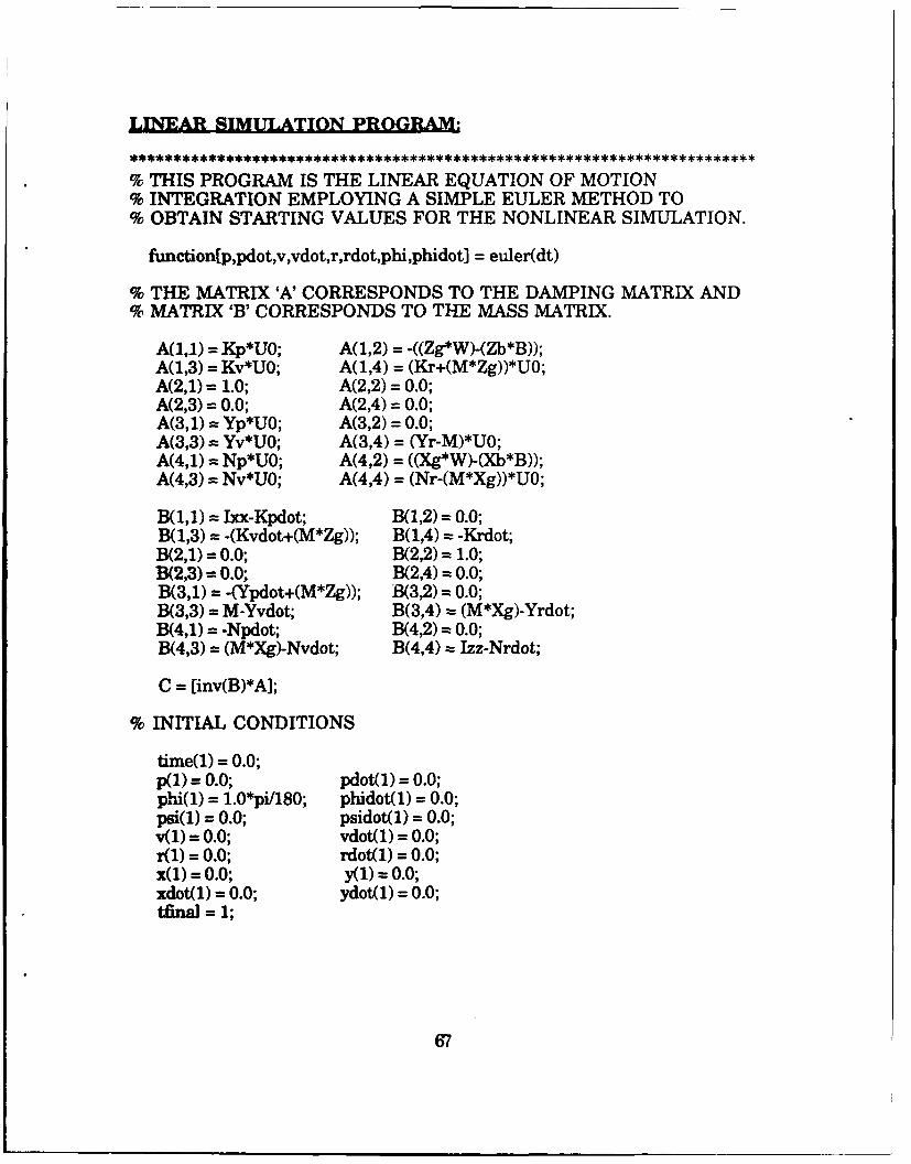
% THIS PROGRAM IS THE LINEAR EQUATION OF MOTION% INTEGRATION EMPLOYING A SIMPLE EULER METHOD TO% OBTAIN STARTING VALUES FOR THE NONLINEAR SIMULATION.
function[p,pdot,v,vdot,r,rdot,phi,phidot] = euler(dt)
% THE MATRIX 'A' CORRESPONDS TO THE DAMPING MATRIX AND% MATRIX 'B' CORRESPONDS TO THE MASS MATRIX.
A(1,U) = Kp*U0; A(1,2) = -((Zg*W)-(Zb*B));A(1,3) = Kv*UO; A(1,4) = (Kr+(M*Zg))*UO;A(2,1) = 1.0; A(2,2) = 0.0;A(2,3) = 0.0; A(2,4) = 0.0;A(3,1) = Yp*UO; A(3,2) = 0.0;A(3,3) = Yv*UO; A(3,4) = (Yr-M)*U0;A(4,1) = Np*U0; A(4,2) = ((Xg*W)-(Xb*B));A(4,3) = Nv*U0; A(4,4) = (Nr-(M*Xg))*U0;
B(1,1) = Ixx-Kpdot; B(1,2) = 0.0;B(1,3) = -(Kvdot+(M*Zg)); B(1,4) = -Krdot;B(2,1) = 0.0; B(2,2) = 1.0;B(2,3) = 0.0; B(2,4) = 0.0;B(3,1) = -(Ypdot+(M*Zg)); B(3,2) = 0.0;B(3,3) = M-Yvdot; B(3,4) (M*Xg)-Yrdot;B(4,1) = -Npdot; B(4,2) 0.0;B(4,3) = (M*Xg)-Nvdot; B(4,4) Izz-Nrdot;
C = [inv(B)*A];
% INITIAL CONDITIONS
time(l) = 0.0;p(l) = 0.0; pdot(1) = 0.0;phi(l) = 1.0*pi/180; phidot(1) = 0.0;psi(l) = 0.0; psidot(1) = 0.0;v(1) = 0.0; vdot(1) = 0.0;r(1) = 0.0; rdot(1) = 0.0;x(1) = 0.0; y(1) = 0.0;xdot(1) = 0.0; ydot(1) = 0.0;tfinal = 1;
67
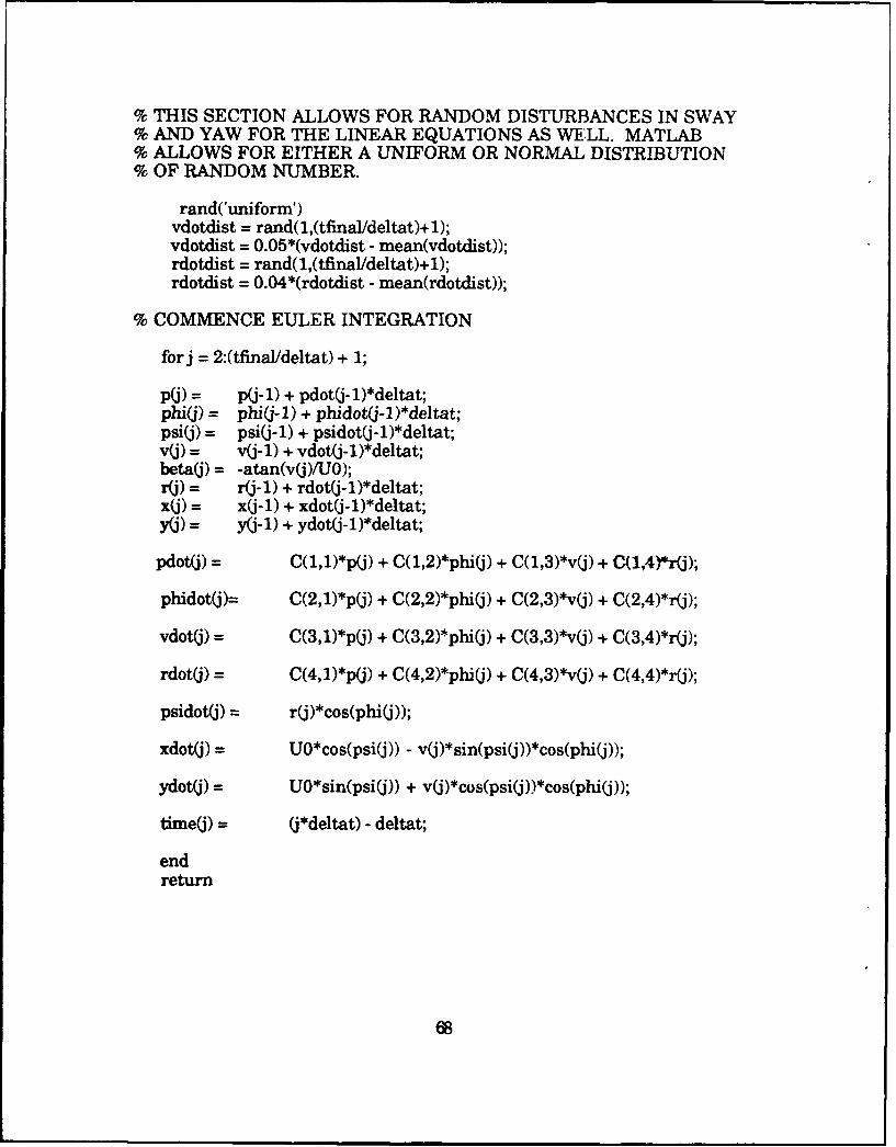
% THIS SECTION ALLOWS FOR RANDOM DISTURBANCES IN SWAY% AND YAW FOR THE LINEAR EQUATIONS AS WELL. MATLAB,% ALLOWS FOR EITHER A UNIFORM OR NORMAL DISTRIBUTION% OF RANDOM NUJMBER.
rand('uniform')vdotdist = rand(l,(tfinalldeltat)+l);vdotdist = O.05*(vdotdist - mean(vdotdist));rdotdist = rand(l,(tfinalldeltat)+l);rdotdist = O.04*(rdotdist - mean(rdotdist));
% COMMENCE EULER INTEGRATION
forj = 2:(tfinal/deltat) + 1;
pQj) = p0j-1) + pdotOj-1)*deltat;phi(j) =phiQj-l) + phidot~j-l)*deltat;psioj) = psioj-1) + psidotQj-1)*deltat;Výj) = voj-1) + vdotoj-1)*deltat;betaOj) =-atan(v(j)/Uo);
r(j) = r(j-1) + rdotQj-1)*deltat;xoj) = xoj-1) + xdotoj-1)*deltat;y(j) = yrj-1) +I ydatQj-1)*deltat;
pdot(j) =C(1,1)*poj) + C(1,2)*phioj) + C(l,3)*vQj) + C(1,4)'*r(j);
phidotoj)= C(2,1)*poj) + C(2,2)*pjh 1jo) + C(2,3)*vQj) + C(2,4)*r(j);
vdotQj) = C(3,1)*pQj) + C(3,2)*phij) + C(3,3)*vQj) + C(3,4)*r~j);
rdotQj) = C(4,1)*pQj) + C(4,2)*phiQj) + C(4,3)*vQj) + C(4,4)*r(j);
psidotoj) =rQj)*cos(phioj));
xdotW) = UO*cos(psioj)) - voj)*sin(psiQj))*cos(phiQj));
ydotkj) = UO*sin(psiQj)) + voj)*cos(psicj))*cos(phioj));
tixneQ) = (*deltat) - deltat;
end
return
68
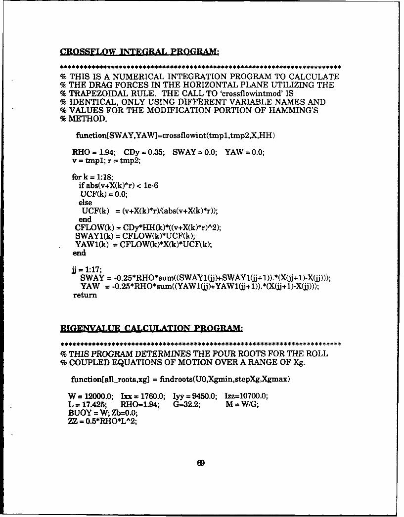
CROSSFLOW INTEGRAL PROGRAM:
% THIS IS A NUMERICAL INTEGRATION PROGRAM TO CALCULATE% THE DRAG FORCES IN THE HORIZONTAL PLANE UTILIZING THE% TRAPEZOIDAL RULE. THE CALL TO 'crossflowintmod' IS% IDENTICAL, ONLY USING DIFFERENT VARIABLE NAMES AND% VALUES FOR THE MODIFICATION PORTION OF HAMMING'S% METHOD.
finction[SWAY,YAW]=crossflowint(tmpl ,tmp2,X,HH)
RHO = 1.94; CDy = 0.35; SWAY = 0.0; YAW = 0.0;v = tznpl; r = tmp2;
for k = 1:18;if abs(v+X(k)*r) < le-6UCF(k) = 0.0;elseUCF(k) = (v+X(k)*r)/(abs(v+X(k)*r));
endCFLOW(k) = CDy*HH(k)*((v+X(k)*r)A2);SWAY1(k) = CFLOW(k)*UCF(k);YAW1(k) = CFLOW(k)*X(k)*UCF(k);end
ii = 1:17;SWAY = -0.25*RHO*sum((SWAY1(jj)+SWAYI(j+1)).*(X(jj+1)-X(jj)));YAW =-0.25*RHO*sum((YAWl(jj)+YAW1(jj+l)).*(X(jj+l)-X(jj)));
return
EIGENVALUE CACULATION PROGRAM:
"% THIS PROGRAM DETERMINES THE FOUR ROOTS FOR THE ROLL
"% COUPLED EQUATIONS OF MOTION OVER A RANGE OF Xg.
function[all-roots,xg] = findroots(UO,Xgmin,stepXg,Xgmax)
W = 12000.0; Ixx = 1760.0; Iyy = 9450.0; Izz=10700.0;L = 17.425; RHO=1.94; G-=32.2; M = W/G;BUOY = W; Zb=0.0;ZZ = 0.5*RHO*LA2;
69
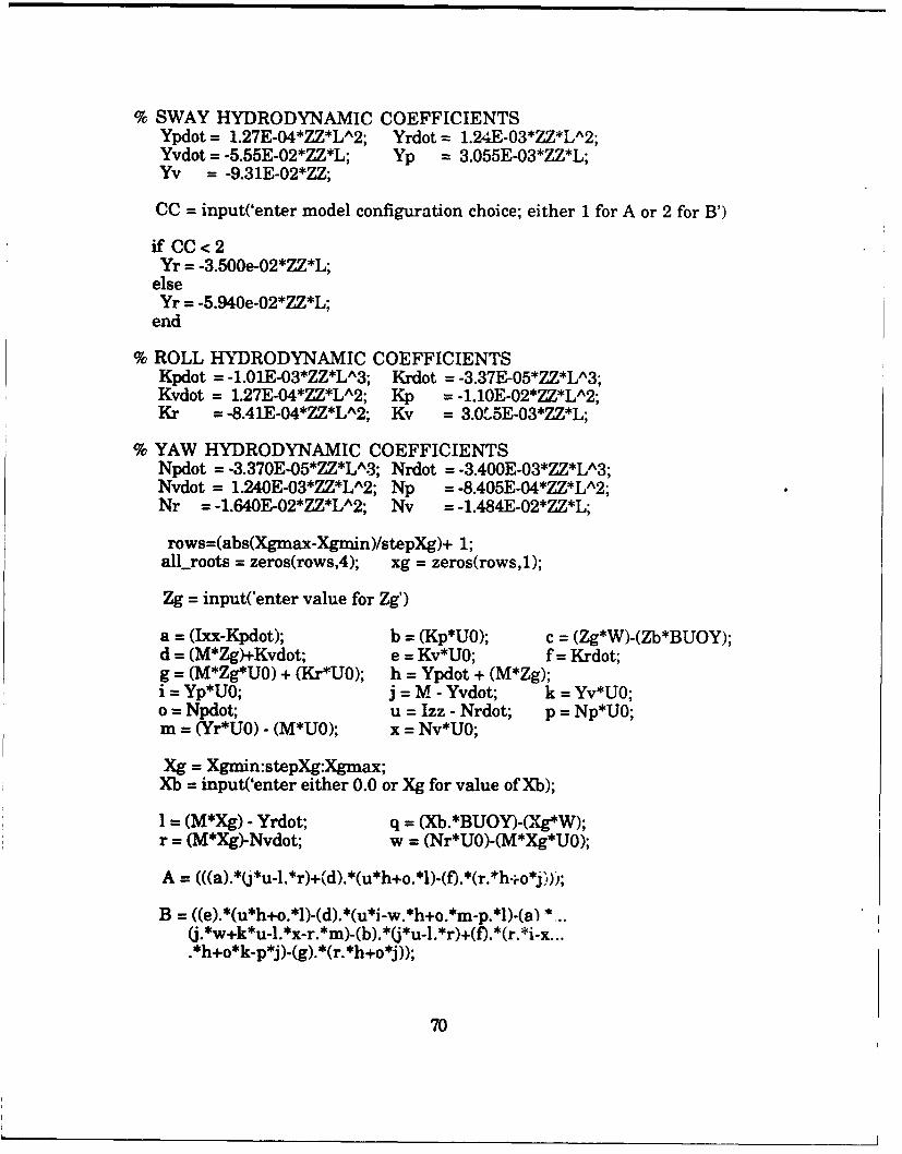
"% SWAY HYDRODYNAMIC COEFFICIENTSYpdot = 1.27E-04*ZZ*L A2; Yrdot = .24E-03*ZZ*LA 2;Yvdot = -5.55E-O2*ZZ*L; Yp =3.O55E-03*ZZ*L;YV -9.31E-O2*ZZ;
CC = input('enter model configuration choice; either 1 for A or 2 for B')
if 00<2Yr = -3.500e.02*ZZ*L;
elseYr = -5.940e.02*ZZ*L;
end
"% ROLL HYDRODYNAMIC COEFFICIENTSKpdot = -1.01E-03*ZZ*LA 3; Krdot = -3.37E-O5*ZZ*L A3;Kvdot = 1.27E-04*ZZ*LA 2; Kp = -1.10E-02*ZZ*L A2;Kr = -8.41E-04*ZZ*LA 2; Ky = 3.O.F5E-03*ZZ*L;
"% YAW HYDRODYNAMIC COEFFICIENTSNpdot = -.3370E405*ZZ*LA 3; Nrdot = -3.400E-03*ZZ*L A3;Nvdot = 1.240E-O3*ZZ*LA 2; Np = -8.4O5E-04*ZZ*L A2;Nr = -1.64OE-O2*ZZ*LA 2; Nv = -1.484E-02*ZZ*L;
rows=(abs(Xgmax-Xgmin)/stepXg)+ 1;all-roots = zeros(rows,4); xg = zeros(rows,1);
Zg = inputCenter value for Zg')
a = (Ixx-Kpdot); b = (Kp*UO); C (Zg*W)-(Zb*BUOY);d = (M*Zg)+Kvdot; e = Kv*UO; f =Krdot;
g = (M*Zg*UO) + (Kr*UO); h = Ypdot + (M*Zg);i = Yp*UO; j =M - Yvdot; k -Yv*UO;
o = Npdot; u Izz - Nrdot; p -Np*UO;
M = (Yr*UO) - (M*UO); x =Nv*UO;
Xg =Xgmin:stepXg:Xgmax;
Xb =input('enter either 0.0 or Xg for value of Xb);
I = (M*Xg) - Yrdot; q =X.BO)('e )r = (M*Xg)-Nvdot; w= (Nr*UO).(M*Xg*UO);
A =(((a).*(J*u-l.*r)+('d).*(u*h+o.*l).(f).*(r. *h..o*j'i)');
B =((e).*(u*h+o.*l)-(d).*(u*i-w.*h+o.*m-p.*l)-(a)(j*w+k*ul.i*x-..*m)-(b).*(*u-l*r)+(f).*(r.*i-...*h+o*k.-p*j)..(g). *(r. *h+o*j));
70
C = ((a).*(k.*w-xn.*x)+(b).*(j.*w+k*u-I. *x-..*m)+(c).*..
o. *m..p.*1)+(f).*(q. *j..x*i+p*k)+(g). *(r. *i-..*h+o*k..
-w. *i+m *p)..(c).*(j.*w+k*u4.*x-..r*m)..(b).*(kL*w-..m*x));
Z= [A' B' CD' E'J;
j = 1:rows; polyfj,:)=zuj,:); Ats = 'roats(poly(jj,:))';
for jj = 1-rows;a]llroots(jj, 1:4) = eval(yts)';end
xg=Xg';end,return
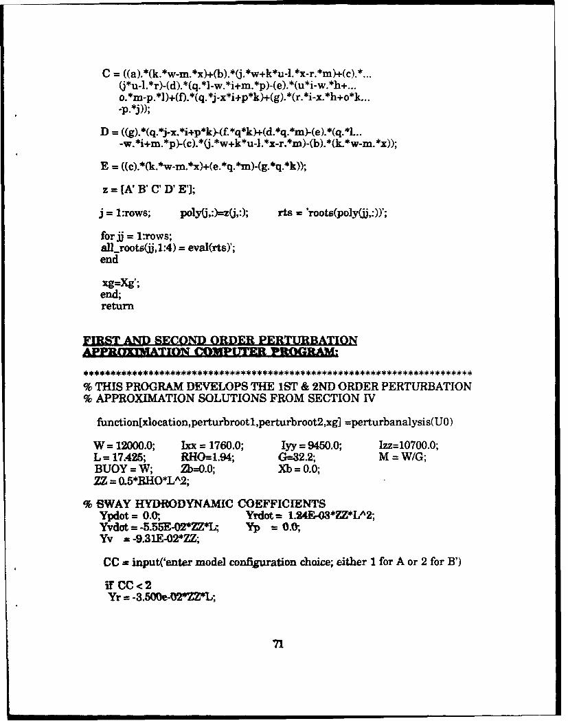
% THIS PROGRAM DEVELOPS THE 1ST & 2ND ORDER PERTURBATION
% APPROXIMATION SOLUTIONS FROM SECTION IV
finction[xlocation,perturbrootl,perturbroot2,xgI =perturbanalysis(UO)
W = 12000.0; lxx = 1760.0; Iyy = 9450.0; Izz= 10700.0;L = 17A426; RHO--1.94; G=32.2; M = WIG;BUOY = W; Zb=0.0; Xb = 0.0;
ZZ= 0.5*REjO*LA2;
% SWAY HYDRODYNAMIC COEFFICIENTSYpdot = 0.0-, Yrdot = 1.24E,03*ZZ*LA2;Yvdcyt = -5.55E-O2*ZZ*L, Y-p = 0.0;,Yv = -9.31E-02*ZZ;
CC = input('enter model configuration choice; either 1 for A or 2 for B')
if CC< 2
Yr = -3.500e-0202Z*L-,
71
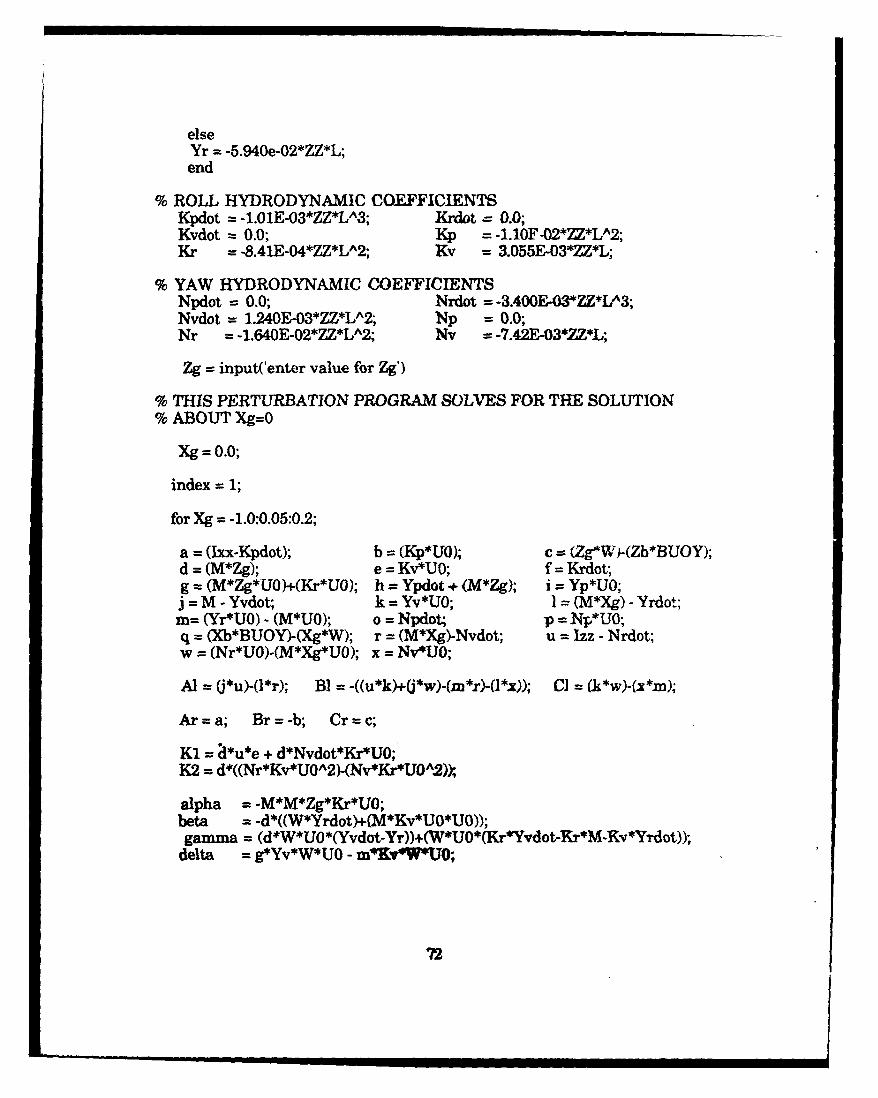
elseYr = -5.940e-02*ZZ*L;end
"% ROLL HYDRODYNAMIC COEFFICIENTSKpdot = l.OlE-03*ZZ*L A3; J•rdot =0.0;Kvdot =0.0; Kp = -1.10F-02*ZZ*LP2;Kr = 841E-4*ZZ*LA2; Ky = 3.055E,03*ZZ*L;
"% YAW HYDRODYNAMIC COEFFICIENTSNpdot =0.0; Nrdot = 3.400E-03*ZZ*LA3;Nvdot = 1.240E,03*ZZ*LA2; Np =0.0;Nr = 1.640E-02*ZZ*LA2; NV = -7.42E-03*ZZ*L;
Zg =input('enter value for Zg')
"% THIS PERTURBATION PROGRAM SOLVES FOR THLE SOLUTION"% ABOUT Xg=0
Xg = 0.0;
index = 1;
for Xg = -1.0:0.05:0.2;
a = (Ixx-Kpdot); b =(Kp*UO); c =(ZgeWF(Zb*BUOY);d = (M*Zg). e = Kv*UO; f = Krdot;g =(M*Zg*'UO)+(Kr*UO); h = Ypdot + (M*zg); i = Yp*U0;j = M - Yvd~ot; k = Yv*U0; I =(M*Xg) - Yrdot;M= (Yr*Uo) - (M*Uo); 0 = Npdot; p =Np*UO;
q (Xfl*BUOY)-(Xg*W); r = (M*Xg)-Nvdot; u Izz - Nrdot;w =(Nr*U0)-(M*Xg*UO); x = Nv41UO;
A] =(U*u)..(l*r); BI = -((u*k)+(j*w)-(m*.r)-(]*x)); C] = (Jk*w)-{x*m);
Ar =a; Br =-b; Cr =c;
K1 = aue+ d*Nvdot*Kr*UO;'K2 = d*((Nr*Kv *UoA 2)-(Nv*Kr*UOA2)Y,
alpha = -M*M*Zg*Kr*UO;beta = -d*((W*Yrdot)+(M*Kv*U0*UO));gamma = (d*W*UO*(Yvdot-Yr))+(W*U0*(Kr*Yvdot'Xr*M-Rv*Yrdot));
delta = g*Yv*W*TJ0 - m*Kv*WUO;
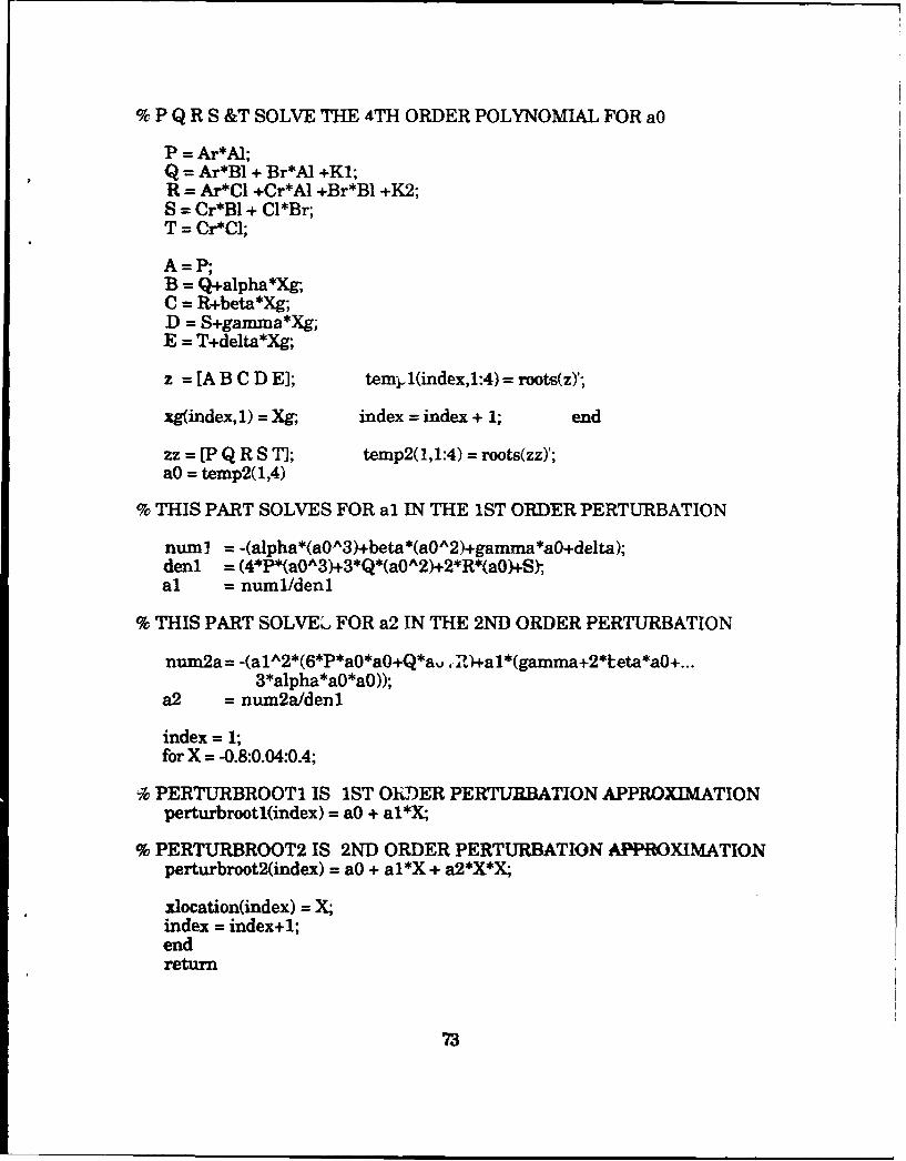
% P Q R S &T SOLVE THE 4TH ORDER POLYNOMIAL FOR aO
Q = Ar*Bl + Br*AI +1(1;R = Ar*CI +Cr*AI +Br*Bl +K(2;S = Cr*Bl + C1*Br;T = Cr*Cl;
A=P;B = Q+alpha*Xg-C = R+beta*Xg;D =S+gamma*Xg;
E =T+delta*Xg;
z =LA B C DEl; temi, (index,1:4)= roots(z)';
xg(index, 1) = Xg; index = index + 1; end
zz = [P Q R S T]; temp2(1,1:4) = roots(zz)';aO = temp2(1,4)
% THIS PART SOLVES FOR al IN THE 1ST ORDER PERTURBATION
num I = -(alpha*(aoA 3)+beta*(aoA 2)+gamlna*aO+delta);deni = (4*P*(aOA3)+3*Q*(aOA2)+2*R*(aO)+S),al = numi/deni
% THIS PART SOLVEL'i FOR a2 IN THE 2ND ORDER PERTURBATION
num2a = -(al A2*(6*P*a0*a0+Q*a.,', Z-+a 1*(gamma+2*keta*aO+...3*alpha*aO*aO));
a2 =nu~m2a/denl
index = 1;for X = -0.8:0.0-4:0.4;
-7 PERTURBROOT1 IS 1ST OII-JER PERTURBATION APPROXIMATIONperturbrootl(index) = aO + al*X;,
% PERTURBROOT2 IS 2ND ORDER PERTURBATION APPROXIMATIONperturbroot2(index) = aO + al*X + a2*X*X,
zlocation(index) = Xindex = index+l;,endreturn
73
LIST OF REFERENCES
1. Yoerger, D.R. and Newman, J.B., "High Performance SupervisoryControl of Vehicles and Manipulators", Intervention '87Conference and Exposition, pages 189-192.
2. Gerald, C.F. and Wheatley, P.O., "Applied Numerical Analysis",Addison-Wesley Publishing Company, Fourth Edition, 1989, p. 384.
3. Smith, N.S., Crane, J.W., and Summey, D.C., "SDV SimulatorHydrodynamic Coefficients", NCSC Technical Memorandum 231-78,June 1978, pages 11-16, 20, 24-31.
4. Dorf, R.C., "Modern Control Systems", Addison-Wesley PublishingCompany, Sixth Edition, 1992.
5. Schmidt, L.V. and Wright, S.R., "Aircraft Wing Rock By InertialCoupling", AIAA-91-2885-CP, August 1991, p. 371.
6. Simmonds, J.G. and Mann, J.E., "A First Look at PerturbationTheory", Robert E. Krieger Publishing Company, 1986, pages 12-38.
BIBLIOGRAPHY
Booth, T.B., "Stability of Buoyant Underwater Vehicles,Predominantly Forward Motion", International ShipbuildingProgress, Volume 24, November 1977, Nr. 279, pages 297-305.
McKinley, B.D., "Dynamic Stability of Positively BuoyantSubmersibles: Vertical Plane Solutions", Master's Thesis, NavalPostgraduate School, Monterey, California, December 1991.
Papoulias, F.A., "Stability and Bifurcations of Towed UnderwaterVehicles in the Dive Plane", Journal of Ship Research, Volume 36,.No. 3, September 1992, pages 255-267.
74

INITIAL DISTRIBUTION LIST
No. CopiesI Defense Technical Information Center 2
Cameron StationAlexandria, Virginia 22304-6145
2a Library, Code 52 2Naval Postgraduate SchoolMonterey, California 93943-5002
3. Department Chairman, Code ME 1Department of Mechanical EngineeringNaval Postgraduate SchoolMonterey, California 93943-5000
4. Professor Fotis A. Papoulias 4Code ME/PaDepartment of Mechanical EngineeringNaval Postgraduate SchoolMonterey, California 93943-5000
5. LT Daniel J. Cunningham, II 258 Case ParkwayBurlington, Vermont 05401
6. Naval Engineering Curricular Officer, Code 34 1Department of Mechanical EngineeringNaval Postgraduate SchoolMonterey, California 93943-5004
75