Embed Size (px)
Citation preview
Journal of Machine Learning Research 12 (2011) 2493-2537 Submitted 1/10; Revised 11/10; Published 8/11
Natural Language Processing (Almost) from Scratch
Ronan Collobert∗ [email protected]
Jason Weston† [email protected]
Leon Bottou‡ [email protected]
Michael Karlen MICHAEL .KARLEN@GMAIL .COM
Koray Kavukcuoglu§ [email protected] .EDU
Pavel Kuksa¶ [email protected]
NEC Laboratories America4 Independence WayPrinceton, NJ 08540
Editor: Michael Collins
AbstractWe propose a unified neural network architecture and learning algorithm that can be applied to var-ious natural language processing tasks including part-of-speech tagging, chunking, named entityrecognition, and semantic role labeling. This versatilityis achieved by trying to avoid task-specificengineering and therefore disregarding a lot of prior knowledge. Instead of exploiting man-madeinput features carefully optimized for each task, our system learns internal representations on thebasis of vast amounts of mostly unlabeled training data. This work is then used as a basis forbuilding a freely available tagging system with good performance and minimal computational re-quirements.Keywords: natural language processing, neural networks
1. Introduction
Will a computer program ever be able to convert a piece of English text into aprogrammer friendlydata structure that describes the meaning of the natural language text? Unfortunately, no consensushas emerged about the form or the existence of such a data structure. Until such fundamentalArticial Intelligence problems are resolved, computer scientists must settle forthe reduced objectiveof extracting simpler representations that describe limited aspects of the textual information.
These simpler representations are often motivated by specific applications (for instance, bag-of-words variants for information retrieval), or by our belief that they capture something more gen-eral about natural language. They can describe syntactic information (e.g., part-of-speech tagging,chunking, and parsing) or semantic information (e.g., word-sense disambiguation, semantic rolelabeling, named entity extraction, and anaphora resolution). Text corpora have been manually an-notated with such data structures in order to compare the performance of various systems. Theavailability of standard benchmarks has stimulated research in Natural Language Processing (NLP)
∗. Ronan Collobert is now with the Idiap Research Institute, Switzerland.†. Jason Weston is now with Google, New York, NY.‡. Leon Bottou is now with Microsoft, Redmond, WA.§. Koray Kavukcuoglu is also with New York University, New York, NY.¶. Pavel Kuksa is also with Rutgers University, New Brunswick, NJ.
c©2011 Ronan Collobert, Jason Weston, Leon Bottou, Michael Karlen, Koray Kavukcuoglu and Pavel Kuksa.
COLLOBERT, WESTON, BOTTOU, KARLEN, KAVUKCUOGLU AND KUKSA
and effective systems have been designed for all these tasks. Such systems are often viewed assoftware components for constructing real-world NLP solutions.
The overwhelming majority of these state-of-the-art systems address their single benchmarktask by applying linear statistical models to ad-hoc features. In other words, the researchers them-selves discover intermediate representations by engineering task-specific features. These featuresare often derived from the output of preexisting systems, leading to complex runtime dependencies.This approach is effective because researchers leverage a large body of linguistic knowledge. Onthe other hand, there is a great temptation to optimize the performance of a system for a specificbenchmark. Although such performance improvements can be very useful in practice, they teach uslittle about the means to progress toward the broader goals of natural language understanding andthe elusive goals of Artificial Intelligence.
In this contribution, we try to excel onmultiple benchmarkswhile avoiding task-specific engi-neering. Instead we use asingle learning systemable to discover adequate internal representations.In fact we view the benchmarks as indirect measurements of the relevanceof the internal represen-tations discovered by the learning procedure, and we posit that these intermediate representationsare more general than any of the benchmarks. Our desire to avoid task-specific engineered featuresprevented us from using a large body of linguistic knowledge. Instead wereach good performancelevels in most of the tasks by transferring intermediate representations discovered on large unlabeleddata sets. We call this approach “almost from scratch” to emphasize the reduced (but still important)reliance on a priori NLP knowledge.
The paper is organized as follows. Section 2 describes the benchmark tasks of interest. Sec-tion 3 describes the unified model and reports benchmark results obtained with supervised training.Section 4 leverages large unlabeled data sets (∼ 852 million words) to train the model on a languagemodeling task. Performance improvements are then demonstrated by transferring the unsupervisedinternal representations into the supervised benchmark models. Section 5 investigates multitasksupervised training. Section 6 then evaluates how much further improvementcan be achieved byincorporating standard NLP task-specific engineering into our systems. Drifting away from our ini-tial goals gives us the opportunity to construct an all-purpose tagger thatis simultaneously accurate,practical, and fast. We then conclude with a short discussion section.
2. The Benchmark Tasks
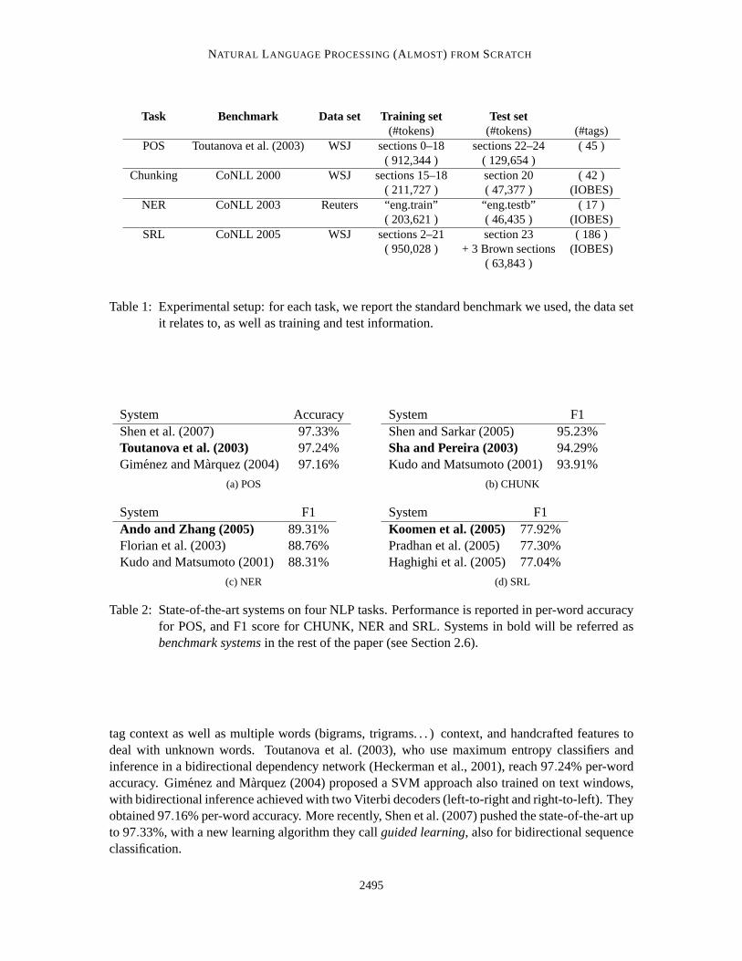
In this section, we briefly introduce four standard NLP tasks on which we will benchmark ourarchitectures within this paper: Part-Of-Speech tagging (POS), chunking (CHUNK), Named EntityRecognition (NER) and Semantic Role Labeling (SRL). For each of them, we consider a standardexperimental setup and give an overview of state-of-the-art systems onthis setup. The experimentalsetups are summarized in Table 1, while state-of-the-art systems are reported in Table 2.
2.1 Part-Of-Speech Tagging
POS aims at labeling each word with a unique tag that indicates itssyntactic role, for example, pluralnoun, adverb, . . . A standard benchmark setup is described in detail byToutanova et al. (2003).Sections 0–18 of Wall Street Journal (WSJ) data are used for training,while sections 19–21 are forvalidation and sections 22–24 for testing.
The best POS classifiers are based on classifiers trained on windows oftext, which are then fedto a bidirectional decoding algorithm during inference. Features include preceding and following
2494
NATURAL LANGUAGE PROCESSING(ALMOST) FROM SCRATCH
Task Benchmark Data set Training set Test set(#tokens) (#tokens) (#tags)
POS Toutanova et al. (2003) WSJ sections 0–18 sections 22–24 (45 )( 912,344 ) ( 129,654 )
Chunking CoNLL 2000 WSJ sections 15–18 section 20 ( 42 )( 211,727 ) ( 47,377 ) (IOBES)
NER CoNLL 2003 Reuters “eng.train” “eng.testb” ( 17 )( 203,621 ) ( 46,435 ) (IOBES)
SRL CoNLL 2005 WSJ sections 2–21 section 23 ( 186 )( 950,028 ) + 3 Brown sections (IOBES)
( 63,843 )
Table 1: Experimental setup: for each task, we report the standard benchmark we used, the data setit relates to, as well as training and test information.
System AccuracyShen et al. (2007) 97.33%Toutanova et al. (2003) 97.24%Gimenez and Marquez (2004) 97.16%
(a) POS
System F1Shen and Sarkar (2005) 95.23%Sha and Pereira (2003) 94.29%Kudo and Matsumoto (2001) 93.91%
(b) CHUNK
System F1Ando and Zhang (2005) 89.31%Florian et al. (2003) 88.76%Kudo and Matsumoto (2001) 88.31%
(c) NER
System F1Koomen et al. (2005) 77.92%Pradhan et al. (2005) 77.30%Haghighi et al. (2005) 77.04%
(d) SRL
Table 2: State-of-the-art systems on four NLP tasks. Performance is reported in per-word accuracyfor POS, and F1 score for CHUNK, NER and SRL. Systems in bold will be referred asbenchmark systemsin the rest of the paper (see Section 2.6).
tag context as well as multiple words (bigrams, trigrams. . . ) context, and handcrafted features todeal with unknown words. Toutanova et al. (2003), who use maximum entropy classifiers andinference in a bidirectional dependency network (Heckerman et al., 2001), reach 97.24% per-wordaccuracy. Gimenez and Marquez (2004) proposed a SVM approach also trained on text windows,with bidirectional inference achieved with two Viterbi decoders (left-to-right and right-to-left). Theyobtained 97.16% per-word accuracy. More recently, Shen et al. (2007) pushedthe state-of-the-art upto 97.33%, with a new learning algorithm they callguided learning, also for bidirectional sequenceclassification.
2495
COLLOBERT, WESTON, BOTTOU, KARLEN, KAVUKCUOGLU AND KUKSA
2.2 Chunking
Also called shallow parsing, chunking aims at labeling segments of a sentencewith syntactic con-stituents such as noun or verb phrases (NP or VP). Each word is assigned only one unique tag, oftenencoded as a begin-chunk (e.g., B-NP) or inside-chunk tag (e.g., I-NP). Chunking is often evaluatedusing the CoNLL 2000 shared task.1 Sections 15–18 of WSJ data are used for training and section20 for testing. Validation is achieved by splitting the training set.
Kudoh and Matsumoto (2000) won the CoNLL 2000 challenge on chunking with a F1-scoreof 93.48%. Their system was based on Support Vector Machines (SVMs). Each SVM was trainedin a pairwise classification manner, and fed with a window around the word ofinterest containingPOS and words as features, as well as surrounding tags. They perform dynamic programming attest time. Later, they improved their results up to 93.91% (Kudo and Matsumoto, 2001) using anensemble of classifiers trained with different tagging conventions (see Section 3.3.3).
Since then, a certain number of systems based on second-order randomfields were reported(Sha and Pereira, 2003; McDonald et al., 2005; Sun et al., 2008), all reporting around 94.3% F1score. These systems use features composed of words, POS tags, andtags.
More recently, Shen and Sarkar (2005) obtained 95.23% using a voting classifier scheme, whereeach classifier is trained on different tag representations2 (IOB, IOE, . . . ). They use POS featurescoming from an external tagger, as well carefully hand-craftedspecializationfeatures which againchange the data representation by concatenating some (carefully chosen) chunk tags or some wordswith their POS representation. They then build trigrams over these features,which are finally passedthrough a Viterbi decoder a test time.
2.3 Named Entity Recognition
NER labels atomic elements in the sentence into categories such as “PERSON” or“LOCATION”.As in the chunking task, each word is assigned a tag prefixed by an indicator of the beginning or theinside of an entity. The CoNLL 2003 setup3 is a NER benchmark data set based on Reuters data.The contest provides training, validation and testing sets.
Florian et al. (2003) presented the best system at the NER CoNLL 2003 challenge, with 88.76%F1 score. They used a combination of various machine-learning classifiers. Features they pickedincluded words, POS tags, CHUNK tags, prefixes and suffixes, a largegazetteer (not provided bythe challenge), as well as the output of two other NER classifiers trained onricher data sets. Chieu(2003), the second best performer of CoNLL 2003 (88.31% F1), also used an external gazetteer(their performance goes down to 86.84% with no gazetteer) and several hand-chosen features.
Later, Ando and Zhang (2005) reached 89.31% F1 with a semi-supervised approach. Theytrained jointly a linear model on NER with a linear model on two auxiliary unsupervised tasks.They also performed Viterbi decoding at test time. The unlabeled corpus was 27M words takenfrom Reuters. Features included words, POS tags, suffixes and prefixes or CHUNK tags, but overallwere less specialized than CoNLL 2003 challengers.
1. Seehttp://www.cnts.ua.ac.be/conll2000/chunking .2. See Table 3 for tagging scheme details.3. Seehttp://www.cnts.ua.ac.be/conll2003/ner .
2496
NATURAL LANGUAGE PROCESSING(ALMOST) FROM SCRATCH
2.4 Semantic Role Labeling
SRL aims at giving a semantic role to a syntactic constituent of a sentence. In the PropBank(Palmer et al., 2005) formalism one assigns roles ARG0-5 to words that arearguments of a verb(or more technically, apredicate) in the sentence, for example, the following sentence might betagged “[John]ARG0 [ate]REL [the apple]ARG1 ”, where “ate” is the predicate. The precise argumentsdepend on a verb’sframeand if there are multiple verbs in a sentence some words might have multi-ple tags. In addition to the ARG0-5 tags, there there are several modifier tags such as ARGM-LOC(locational) and ARGM-TMP (temporal) that operate in a similar way for all verbs. We pickedCoNLL 20054 as our SRL benchmark. It takes sections 2–21 of WSJ data as training set,and sec-tion 24 as validation set. A test set composed of section 23 of WSJ concatenated with 3 sectionsfrom the Brown corpus is also provided by the challenge.
State-of-the-art SRL systems consist of several stages: producing aparse tree, identifying whichparse tree nodes represent the arguments of a given verb, and finallyclassifying these nodes tocompute the corresponding SRL tags. This entails extracting numerous basefeatures from the parsetree and feeding them into statistical models. Feature categories commonly usedby these systeminclude (Gildea and Jurafsky, 2002; Pradhan et al., 2004):
• the parts of speech and syntactic labels of words and nodes in the tree;
• the node’s position (left or right) in relation to the verb;
• the syntactic path to the verb in the parse tree;
• whether a node in the parse tree is part of a noun or verb phrase;
• the voice of the sentence: active or passive;
• the node’s head word; and
• the verb sub-categorization.
Pradhan et al. (2004) take these base features and define additional features, notably the part-of-speech tag of the head word, the predicted named entity class of the argument, features providingword sense disambiguation for the verb (they add 25 variants of 12 new feature types overall). Thissystem is close to the state-of-the-art in performance. Pradhan et al. (2005) obtain 77.30% F1 with asystem based on SVM classifiers and simultaneously using the two parse trees provided for the SRLtask. In the same spirit, Haghighi et al. (2005) use log-linear models on each tree node, re-rankedglobally with a dynamic algorithm. Their system reaches 77.04% using the five top Charniak parsetrees.
Koomen et al. (2005) hold the state-of-the-art with Winnow-like (Littlestone,1988) classifiers,followed by a decoding stage based on an integer program that enforces specific constraints on SRLtags. They reach 77.92% F1 on CoNLL 2005, thanks to the five top parse trees produced by theCharniak (2000) parser (only the first one was provided by the contest) as well as the Collins (1999)parse tree.
4. Seehttp://www.lsi.upc.edu/ ˜ srlconll .
2497
COLLOBERT, WESTON, BOTTOU, KARLEN, KAVUKCUOGLU AND KUKSA
2.5 Evaluation
In our experiments, we strictly followed the standard evaluation procedureof each CoNLL chal-lenges for NER, CHUNK and SRL. In particular, we chose the hyper-parameters of our modelaccording to a simple validation procedure (see Remark 8 later in Section 3.5),performed over thevalidation set available for each task (see Section 2). All these three tasksare evaluated by comput-ing the F1 scores overchunksproduced by our models. The POS task is evaluated by computingthe per-wordaccuracy, as it is the case for the standard benchmark we refer to (Toutanova et al.,2003). We used theconlleval script5 for evaluating POS,6 NER and CHUNK. For SRL, we usedthesrl-eval.pl script included in thesrlconll package.7
2.6 Discussion
When participating in an (open) challenge, it is legitimate to increase generalization by all means.It is thus not surprising to see many top CoNLL systems usingexternal labeled data, like additionalNER classifiers for the NER architecture of Florian et al. (2003) or additional parse trees for SRLsystems (Koomen et al., 2005). Combining multiple systems or tweaking carefully features is alsoa common approach, like in the chunking top system (Shen and Sarkar, 2005).
However, whencomparingsystems, we do not learn anything of the quality of each system ifthey were trained withdifferent labeled data. For that reason, we will refer tobenchmark systems,that is, top existing systems which avoid usage of external data and have been well-established inthe NLP field: Toutanova et al. (2003) for POS and Sha and Pereira (2003) for chunking. For NERwe consider Ando and Zhang (2005) as they were using additionalunlabeleddata only. We pickedKoomen et al. (2005) for SRL, keeping in mind they use 4 additional parse trees not provided bythe challenge. These benchmark systems will serve as baseline references in our experiments. Wemarked them in bold in Table 2.
We note that for the four tasks we are considering in this work, it can be seen that for themore complex tasks (with corresponding lower accuracies), the best systems proposed have moreengineered features relative to the best systems on the simpler tasks. Thatis, the POS task is one ofthe simplest of our four tasks, and only has relatively few engineered features, whereas SRL is themost complex, and many kinds of features have been designed for it. This clearly has implicationsfor as yet unsolved NLP tasks requiring more sophisticated semantic understanding than the onesconsidered here.
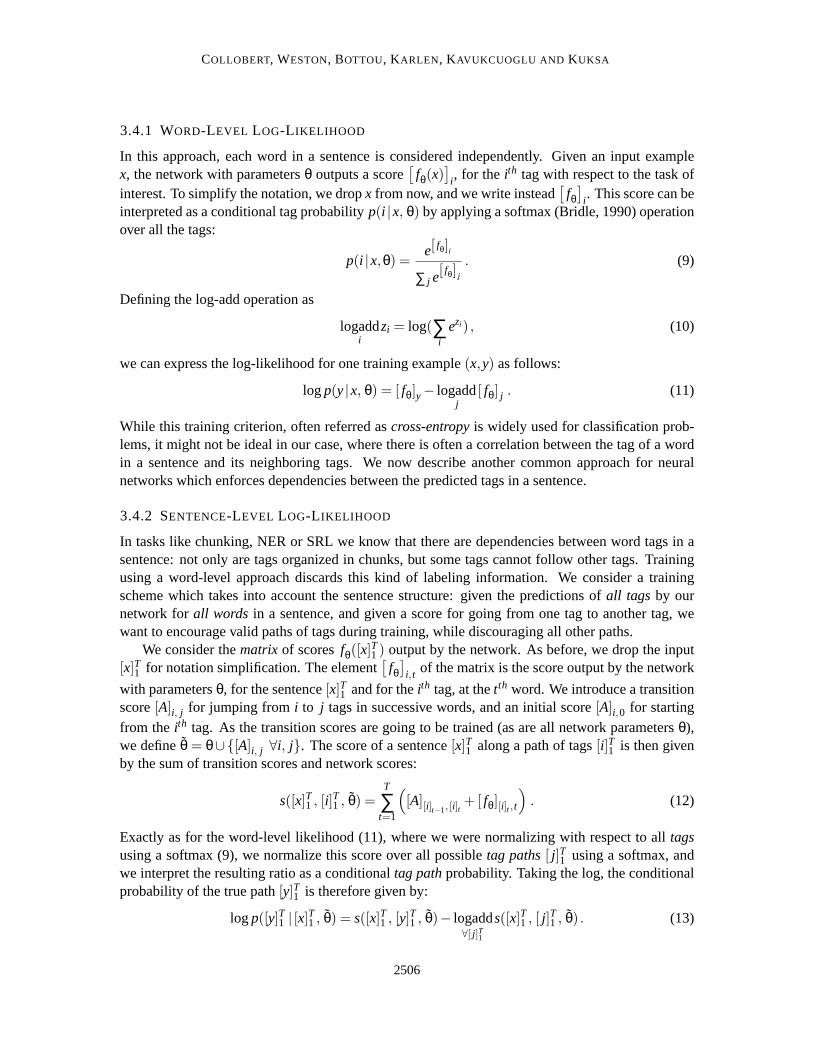
3. The Networks
All the NLP tasks above can be seen as tasks assigning labels to words. The traditional NLP ap-proach is: extract from the sentence a rich set of hand-designed features which are then fed to astandard classification algorithm, for example, a Support Vector Machine (SVM), often with a lin-ear kernel. The choice of features is a completely empirical process, mainly based first on linguisticintuition, and then trial and error, and the feature selection is task dependent, implying additionalresearch for each new NLP task. Complex tasks like SRL then require a large number of possibly
5. Available athttp://www.cnts.ua.ac.be/conll2000/chunking/conllev al.txt .6. We used the “-r ” option of theconlleval script to get the per-word accuracy, for POS only.7. Available athttp://www.lsi.upc.es/ ˜ srlconll/srlconll-1.1.tgz .
2498
NATURAL LANGUAGE PROCESSING(ALMOST) FROM SCRATCH
Input Window
Lookup Table
Linear
HardTanh
Linear
Text cat sat on the mat
Feature 1 w1
1w
1
2 . . . w1
N...
Feature K wK1
wK2 . . . w
K
N
LTW 1xxxxxxxxxxxxxxxxxxxxxxxxxxxxxxxxxxxxxxxxxxxxxxxxxx...
LTW KxxxxxxxxxxxxxxxxxxxxM
1× ·
M2× ·
word of interest
d
concatxxxxxxxxxxxxxxxxxxxxxxxxxxxxxxn1huxxxxxxxxxxxxxxxxxxxxxxxxxxxxxxxxxxxxxxxxxxxxxxxn
2hu
= #tags
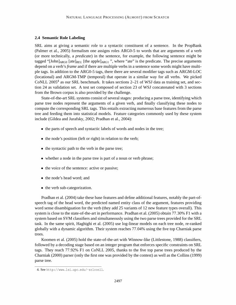
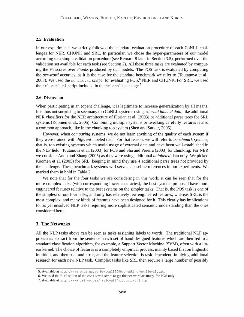
Figure 1: Window approach network.
complex features (e.g., extracted from a parse tree) which can impact the computational cost whichmight be important for large-scale applications or applications requiring real-time response.
Instead, we advocate a radically different approach: as input we will try to pre-process ourfeatures as little as possible and then use a multilayer neural network (NN) architecture, trained inan end-to-end fashion. The architecture takes the input sentence and learns several layers of featureextraction that process the inputs. The features computed by the deep layers of the network areautomatically trained by backpropagation to be relevant to the task. We describe in this section ageneral multilayer architecture suitable for all our NLP tasks, which is generalizable to other NLPtasks as well.
Our architecture is summarized in Figure 1 and Figure 2. The first layer extracts features foreach word. The second layer extracts features from a window of words or from the whole sentence,treating it as asequencewith local and global structure (i.e., it is not treated like a bag of words).The following layers are standard NN layers.
3.1 Notations
We consider a neural networkfθ(·), with parametersθ. Any feed-forward neural network withLlayers, can be seen as a composition of functionsf l
θ(·), corresponding to each layerl :
fθ(·) = f Lθ ( f L−1
θ (. . . f 1θ (·) . . .)) .
2499
COLLOBERT, WESTON, BOTTOU, KARLEN, KAVUKCUOGLU AND KUKSA
Input Sentence
Lookup Table
Convolution
Max Over Time
Linear
HardTanh
Linear
Text The cat sat on the mat
Feature 1 w1
1w
1
2 . . . w1
N...
Feature K wK1
wK2 . . . w
K
N
LTW 1xxxxxxxxxxxxxxxxxxxxxxxxxxxxxxxxxxxxxxxxxxxxxxxxxxxxxxxxxxxxxxxxxxxxxxxxxxxxxxxxxxxxxxxxxx...
LTW Kxxxxxxxxxxxxxxxxxxxxxxxxxxxxxxxxxxxxxxxxxxxxxxxxxxxxxxxxxxxxxxxxxxxxxxxxxxxxxxxxxxxxxxxxxxxxxxxxxxxxxxxxxxxxxxxxxxxxxxxxxxxxxxxxxxxxxxxxxxxxxxxxxxxxxxxxxxxxxxxmax(·)
M2× ·
M3× ·
d
Paddin
g
Paddin
g
n1hu
M1× ·xxxxxxxxxxxxxxxxxxxxn1huxxxxxxxxxxxxxxxxxxxxxxxxxxxxxxxxxx
n2huxxxxxxxxxxxxxxxxxxxxxxxxxxxxxxxxxxxxxxxxxxxxxxxxxxxxxxxxxxxxxn
3hu
= #tags
Figure 2: Sentence approach network.
In the following, we will describe each layer we use in our networks shownin Figure 1 and Figure 2.We adopt few notations. Given a matrixA we denote[A]i, j the coefficient at rowi and columnj
in the matrix. We also denote〈A〉dwini the vector obtained by concatenating thedwin column vectors
around theith column vector of matrixA∈ Rd1×d2:
[
〈A〉dwini
]T
=(
[A]1, i−dwin/2 . . . [A]d1, i−dwin/2 , . . . , [A]1, i+dwin/2 . . . [A]d1, i+dwin/2
)
.
2500
NATURAL LANGUAGE PROCESSING(ALMOST) FROM SCRATCH
As a special case,〈A〉1i represents theith column of matrixA. For a vectorv, we denote[v]i thescalar at indexi in the vector. Finally, a sequence of element{x1, x2, . . . , xT} is written[x]T1 . Theith
element of the sequence is[x]i .
3.2 Transforming Words into Feature Vectors
One of the key points of our architecture is its ability to perform well with the useof (almost8)raw words. The ability for our method to learn good word representations is thus crucial to ourapproach. For efficiency, words are fed to our architecture as indices taken from a finite dictionaryD. Obviously, a simple index does not carry much useful information about the word. However,the first layer of our network maps each of these word indices into a feature vector, by a lookuptable operation. Given a task of interest, a relevant representation of each word is then given bythe corresponding lookup table feature vector, which istrained by backpropagation, starting froma random initialization.9 We will see in Section 4 that we can learn very good word representa-tions from unlabeled corpora. Our architecture allow us to take advantageof better trained wordrepresentations, by simply initializing the word lookup table with these representations (instead ofrandomly).
More formally, for each wordw∈D, an internaldwrd-dimensional feature vector representationis given by thelookup tablelayerLTW(·):
LTW(w) = 〈W〉1w ,
whereW ∈ Rdwrd×|D| is a matrix of parameters to be learned,〈W〉1w ∈ R
dwrd is thewth column ofWanddwrd is the word vector size (a hyper-parameter to be chosen by the user). Given a sentence orany sequence ofT words[w]T1 in D, the lookup table layer applies the same operation for each wordin the sequence, producing the following output matrix:
LTW([w]T1 ) =(
〈W〉1[w]1〈W〉1[w]2
. . . 〈W〉1[w]T
)
. (1)
This matrix can then be fed to further neural network layers, as we will seebelow.
3.2.1 EXTENDING TO ANY DISCRETEFEATURES
One might want to provide features other than words if one suspects that these features are helpfulfor the task of interest. For example, for the NER task, one could provide afeature which says if aword is in a gazetteer or not. Another common practice is to introduce some basicpre-processing,such as word-stemming or dealing with upper and lower case. In this latter option, the word wouldbe then represented by three discrete features: its lower case stemmed root, its lower case ending,and a capitalization feature.
Generally speaking, we can consider a word as represented byK discrete featuresw ∈ D1×·· ·×DK , whereDk is the dictionary for thekth feature. We associate to each feature a lookup tableLTWk(·), with parametersWk ∈ R
dkwrd×|D
k| wheredkwrd ∈ N is a user-specified vector size. Given a
8. We did some pre-processing, namely lowercasing and encoding capitalization as another feature. With enough (un-labeled) training data, presumably we could learn a model without this processing. Ideally, an even more raw inputwould be to learn from letter sequences rather than words, however we felt that this was beyond the scope of thiswork.
9. As any other neural network layer.
2501
COLLOBERT, WESTON, BOTTOU, KARLEN, KAVUKCUOGLU AND KUKSA
word w, a feature vector of dimensiondwrd = ∑k dkwrd is then obtained by concatenating all lookup
table outputs:
LTW1,...,WK (w) =
LTW1(w1)...
LTWK (wK)
=
〈W1〉1w1...
〈WK〉1wK
.
The matrix output of the lookup table layer for a sequence of words[w]T1 is then similar to (1), butwhere extra rows have been added for each discrete feature:
LTW1,...,WK ([w]T1 ) =
〈W1〉1[w1]1. . . 〈W1〉1[w1]T
......
〈WK〉1[wK ]1. . . 〈WK〉1[wK ]T
. (2)
These vector features in the lookup table effectively learn features forwords in the dictionary. Now,we want to use these trainable features as input to further layers of trainable feature extractors, thatcan represent groups of words and then finally sentences.
3.3 Extracting Higher Level Features from Word Feature Vectors
Feature vectors produced by the lookup table layer need to be combined in subsequent layers ofthe neural network to produce a tag decision for each word in the sentence. Producing tags foreach element in variable length sequences (here, a sentence is a sequence of words) is a standardproblem in machine-learning. We consider two common approaches which tagone word at thetime: a window approach, and a (convolutional) sentence approach.
3.3.1 WINDOW APPROACH
A window approach assumes the tag of a word depends mainly on its neighboring words. Given aword to tag, we consider a fixed sizeksz (a hyper-parameter) window of words around this word.Each word in the window is first passed through the lookup table layer (1) or (2), producing a matrixof word features of fixed sizedwrd×ksz. This matrix can be viewed as adwrd ksz-dimensional vectorby concatenating each column vector, which can be fed to further neuralnetwork layers. Moreformally, the word feature window given by the first network layer can bewritten as:
f 1θ = 〈LTW([w]T1 )〉
dwint =
〈W〉1[w]t−dwin/2
...〈W〉1[w]t
...〈W〉1[w]t+dwin/2
. (3)
Linear Layer.The fixed size vectorf 1θ can be fed to one or several standard neural network layers
which perform affine transformations over their inputs:
f lθ =Wl f l−1
θ + bl , (4)
whereWl ∈ Rnl
hu×nl−1hu andbl ∈ R
nlhu are the parameters to betrained. The hyper-parameternl
hu isusually called thenumber of hidden unitsof the l th layer.
2502
NATURAL LANGUAGE PROCESSING(ALMOST) FROM SCRATCH
HardTanh Layer.Several linear layers are often stacked, interleaved with a non-linearity func-tion, to extract highly non-linear features. If no non-linearity is introduced, our network would be asimple linear model. We chose a “hard” version of the hyperbolic tangent asnon-linearity. It has theadvantage of being slightly cheaper to compute (compared to the exact hyperbolic tangent), whileleaving the generalization performance unchanged (Collobert, 2004). The corresponding layerlapplies a HardTanh over its input vector:
[
f lθ
]
i= HardTanh(
[
f l−1θ
]
i) ,
where
HardTanh(x) =
−1 if x<−1x if −1<= x<= 11 if x> 1
. (5)
Scoring. Finally, the output size of the last layerL of our network is equal to the numberof possible tags for the task of interest. Each output can be then interpreted as ascoreof thecorresponding tag (given the input of the network), thanks to a carefully chosen cost function thatwe will describe later in this section.
Remark 1 (Border Effects) The feature window (3) is not well defined for words near the begin-ning or the end of a sentence. To circumvent this problem, we augment the sentence with a special“PADDING” word replicated dwin/2 times at the beginning and the end. This is akin to the use of“start” and “stop” symbols in sequence models.
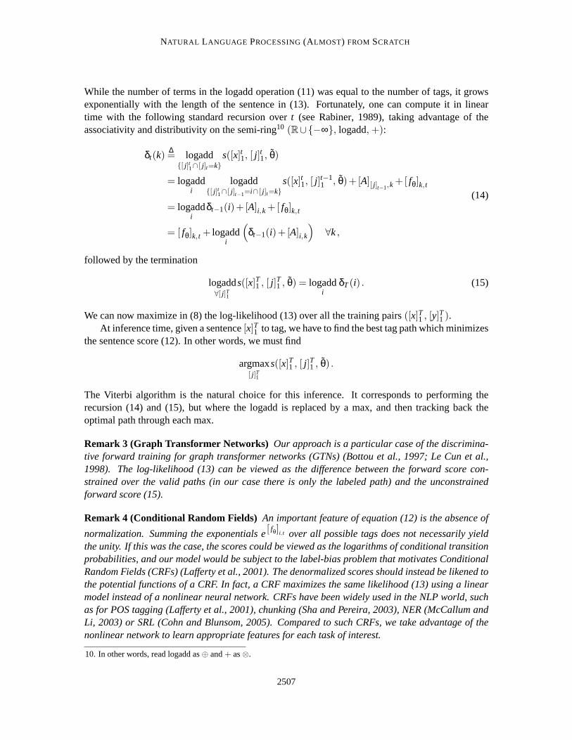
3.3.2 SENTENCEAPPROACH
We will see in the experimental section that a window approach performs wellfor most naturallanguage processing tasks we are interested in. However this approachfails with SRL, where the tagof a word depends on a verb (or, more correctly, predicate) chosen beforehand in the sentence. If theverb falls outside the window, one cannot expect this word to be tagged correctly. In this particularcase, tagging a word requires the consideration of thewholesentence. When using neural networks,the natural choice to tackle this problem becomes a convolutional approach, first introduced byWaibel et al. (1989) and also called Time Delay Neural Networks (TDNNs)in the literature.
We describe in detail our convolutional network below. It successivelytakes the complete sen-tence, passes it through the lookup table layer (1), produces local features around each word of thesentence thanks to convolutional layers, combines these feature into a global feature vector whichcan then be fed to standard affine layers (4). In the semantic role labeling case, this operation isperformed for each word in the sentence, and for each verb in the sentence. It is thus necessary toencode in the network architecture which verb we are considering in the sentence, and which wordwe want to tag. For that purpose, each word at positioni in the sentence is augmented with twofeatures in the way described in Section 3.2.1. These features encode therelative distancesi− posvandi− posw with respect to the chosen verb at positionposv, and the word to tag at positionposwrespectively.
Convolutional Layer.A convolutional layer can be seen as a generalization of a window ap-proach: given a sequence represented by columns in a matrixf l−1
θ (in our lookup table matrix (1)),a matrix-vector operation as in (4) is applied to each window of successivewindows in the sequence.
2503
COLLOBERT, WESTON, BOTTOU, KARLEN, KAVUKCUOGLU AND KUKSA
0
10
20
30
40
50
60
70
Theproposed
changes
alsowould
allowexecutives
to report
exercises
of options
laterand
lessoften
.xxxxxxxxxx
xxxxxxxxxxxxxxxxxx
xxxxxxxxxxx
xxxxxx
xxxxxx
xxxxxx
xxxxxxxxxxxxxx
xxxx
xxxx
xxxxxxxxxxxxxxxxx
xx 0
10
20
30
40
50
60
70
Theproposed
changes
alsowould
allowexecutives
to report
exercises
of options
laterand
lessoften
.xxxxxxxxxx
xxxxxxxxxxxxxxxxxxxxxxxxxx
xxxxx
xxxxxx
xxxxxx
xxxxxxxxxxxxxxxx
xxxxxxxxxxxxxxxxxxxx
xxxxxxxxxxxxxxxxxxxx
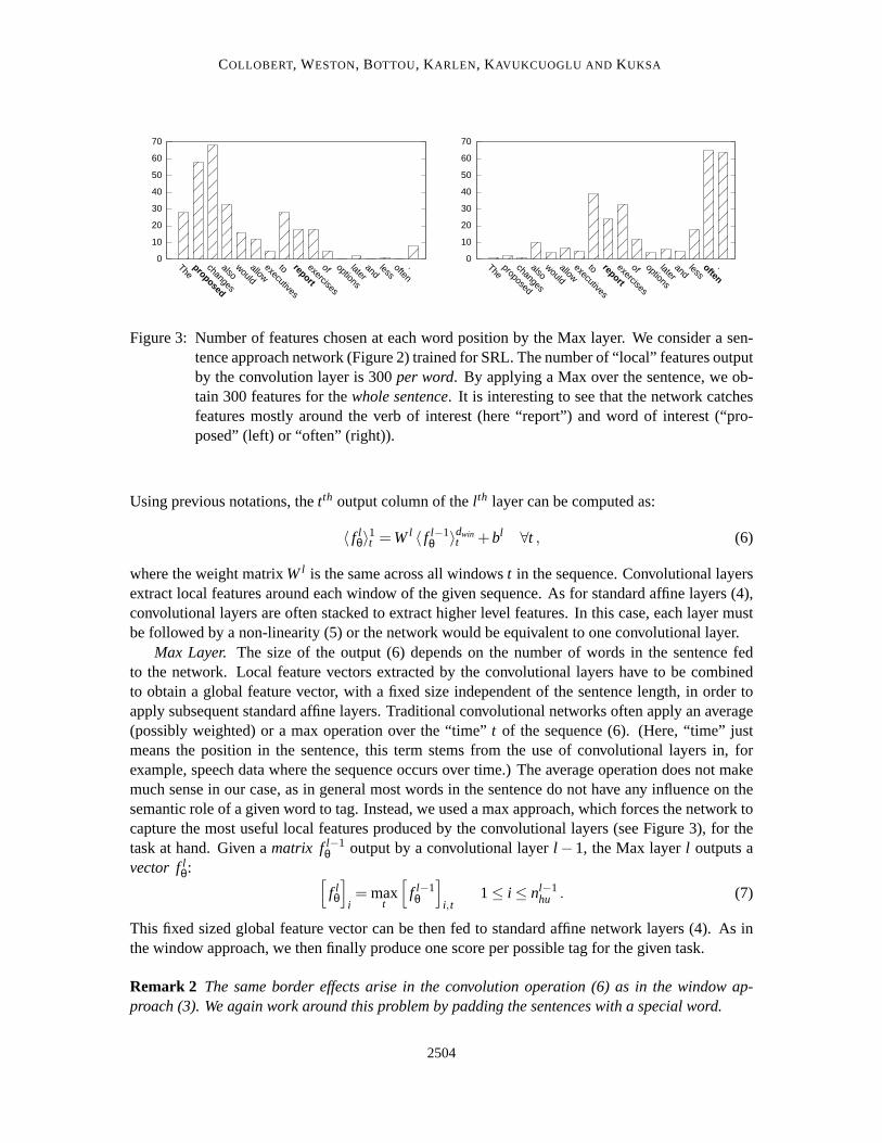
Figure 3: Number of features chosen at each word position by the Max layer. We consider a sen-tence approach network (Figure 2) trained for SRL. The number of “local” features outputby the convolution layer is 300per word. By applying a Max over the sentence, we ob-tain 300 features for thewhole sentence. It is interesting to see that the network catchesfeatures mostly around the verb of interest (here “report”) and word of interest (“pro-posed” (left) or “often” (right)).
Using previous notations, thetth output column of thel th layer can be computed as:
〈 f lθ〉
1t =Wl 〈 f l−1
θ 〉dwint +bl ∀t , (6)
where the weight matrixWl is the same across all windowst in the sequence. Convolutional layersextract local features around each window of the given sequence. As for standard affine layers (4),convolutional layers are often stacked to extract higher level features. In this case, each layer mustbe followed by a non-linearity (5) or the network would be equivalent to one convolutional layer.
Max Layer. The size of the output (6) depends on the number of words in the sentencefedto the network. Local feature vectors extracted by the convolutional layers have to be combinedto obtain a global feature vector, with a fixed size independent of the sentence length, in order toapply subsequent standard affine layers. Traditional convolutional networks often apply an average(possibly weighted) or a max operation over the “time”t of the sequence (6). (Here, “time” justmeans the position in the sentence, this term stems from the use of convolutionallayers in, forexample, speech data where the sequence occurs over time.) The average operation does not makemuch sense in our case, as in general most words in the sentence do not have any influence on thesemantic role of a given word to tag. Instead, we used a max approach, which forces the network tocapture the most useful local features produced by the convolutional layers (see Figure 3), for thetask at hand. Given amatrix fl−1
θ output by a convolutional layerl −1, the Max layerl outputs avector flθ:
[
f lθ
]
i= max
t
[
f l−1θ
]
i, t1≤ i ≤ nl−1
hu . (7)
This fixed sized global feature vector can be then fed to standard affinenetwork layers (4). As inthe window approach, we then finally produce one score per possible tagfor the given task.
Remark 2 The same border effects arise in the convolution operation (6) as in the window ap-proach (3). We again work around this problem by padding the sentences with a special word.
2504
NATURAL LANGUAGE PROCESSING(ALMOST) FROM SCRATCH
Scheme Begin Inside End Single OtherIOB B-X I-X I-X B-X OIOE I-X I-X E-X E-X OIOBES B-X I-X E-X S-X O
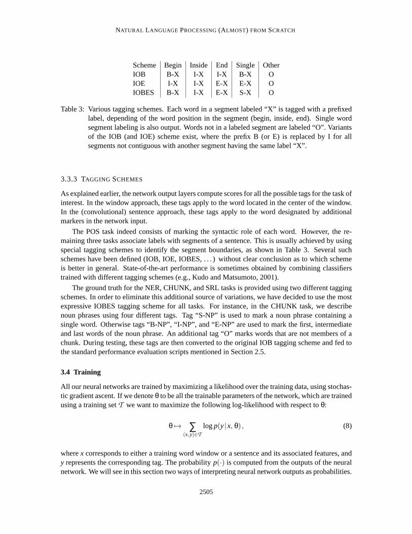
Table 3: Various tagging schemes. Each word in a segment labeled “X” is tagged with a prefixedlabel, depending of the word position in the segment (begin, inside, end). Single wordsegment labeling is also output. Words not in a labeled segment are labeled “O”. Variantsof the IOB (and IOE) scheme exist, where the prefix B (or E) is replaced by I for allsegments not contiguous with another segment having the same label “X”.
3.3.3 TAGGING SCHEMES
As explained earlier, the network output layers compute scores for all thepossible tags for the task ofinterest. In the window approach, these tags apply to the word located in the center of the window.In the (convolutional) sentence approach, these tags apply to the word designated by additionalmarkers in the network input.
The POS task indeed consists of marking the syntactic role of each word. However, the re-maining three tasks associate labels with segments of a sentence. This is usuallyachieved by usingspecial tagging schemes to identify the segment boundaries, as shown in Table 3. Several suchschemes have been defined (IOB, IOE, IOBES, . . . ) without clear conclusion as to which schemeis better in general. State-of-the-art performance is sometimes obtained by combining classifierstrained with different tagging schemes (e.g., Kudo and Matsumoto, 2001).
The ground truth for the NER, CHUNK, and SRL tasks is provided using twodifferent taggingschemes. In order to eliminate this additional source of variations, we have decided to use the mostexpressive IOBES tagging scheme for all tasks. For instance, in the CHUNK task, we describenoun phrases using four different tags. Tag “S-NP” is used to mark a noun phrase containing asingle word. Otherwise tags “B-NP”, “I-NP”, and “E-NP” are used to mark the first, intermediateand last words of the noun phrase. An additional tag “O” marks words that are not members of achunk. During testing, these tags are then converted to the original IOB tagging scheme and fed tothe standard performance evaluation scripts mentioned in Section 2.5.
3.4 Training
All our neural networks are trained by maximizing a likelihood over the trainingdata, using stochas-tic gradient ascent. If we denoteθ to be all the trainable parameters of the network, which are trainedusing a training setT we want to maximize the following log-likelihood with respect toθ:
θ 7→ ∑(x,y)∈T
logp(y|x, θ) , (8)
wherex corresponds to either a training word window or a sentence and its associated features, andy represents the corresponding tag. The probabilityp(·) is computed from the outputs of the neuralnetwork. We will see in this section two ways of interpreting neural network outputs as probabilities.
2505
COLLOBERT, WESTON, BOTTOU, KARLEN, KAVUKCUOGLU AND KUKSA
3.4.1 WORD-LEVEL LOG-L IKELIHOOD
In this approach, each word in a sentence is considered independently.Given an input examplex, the network with parametersθ outputs a score
[fθ(x)
]
i , for the ith tag with respect to the task ofinterest. To simplify the notation, we dropx from now, and we write instead
[fθ]
i . This score can beinterpreted as a conditional tag probabilityp(i |x, θ) by applying a softmax (Bridle, 1990) operationover all the tags:
p(i |x,θ) =e[ fθ]i
∑ j e[ fθ] j
. (9)
Defining the log-add operation as
logaddi
zi = log(∑i
ezi ) , (10)
we can express the log-likelihood for one training example(x,y) as follows:
logp(y|x, θ) = [ fθ]y− logaddj
[ fθ] j . (11)
While this training criterion, often referred ascross-entropyis widely used for classification prob-lems, it might not be ideal in our case, where there is often a correlation between the tag of a wordin a sentence and its neighboring tags. We now describe another common approach for neuralnetworks which enforces dependencies between the predicted tags in a sentence.
3.4.2 SENTENCE-LEVEL LOG-L IKELIHOOD
In tasks like chunking, NER or SRL we know that there are dependenciesbetween word tags in asentence: not only are tags organized in chunks, but some tags cannotfollow other tags. Trainingusing a word-level approach discards this kind of labeling information. Weconsider a trainingscheme which takes into account the sentence structure: given the predictions of all tags by ournetwork forall words in a sentence, and given a score for going from one tag to another tag, wewant to encourage valid paths of tags during training, while discouraging all other paths.
We consider thematrix of scoresfθ([x]T1 ) output by the network. As before, we drop the input
[x]T1 for notation simplification. The element[
fθ]
i, t of the matrix is the score output by the network
with parametersθ, for the sentence[x]T1 and for theith tag, at thetth word. We introduce a transitionscore[A]i, j for jumping fromi to j tags in successive words, and an initial score[A]i,0 for starting
from theith tag. As the transition scores are going to be trained (as are all network parametersθ),we defineθ = θ∪{[A]i, j ∀i, j}. The score of a sentence[x]T1 along a path of tags[i]T1 is then givenby the sum of transition scores and network scores:
s([x]T1 , [i]T1 , θ) =
T
∑t=1
(
[A][i]t−1, [i]t+[ fθ][i]t , t
)
. (12)
Exactly as for the word-level likelihood (11), where we were normalizing withrespect to alltagsusing a softmax (9), we normalize this score over all possibletag paths[ j]T1 using a softmax, andwe interpret the resulting ratio as a conditionaltag pathprobability. Taking the log, the conditionalprobability of the true path[y]T1 is therefore given by:
logp([y]T1 | [x]T1 , θ) = s([x]T1 , [y]
T1 , θ)− logadd
∀[ j]T1
s([x]T1 , [ j]T1 , θ) . (13)
2506
NATURAL LANGUAGE PROCESSING(ALMOST) FROM SCRATCH
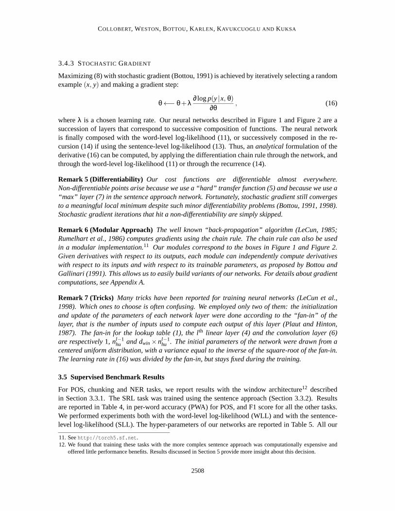
While the number of terms in the logadd operation (11) was equal to the number of tags, it growsexponentially with the length of the sentence in (13). Fortunately, one can compute it in lineartime with the following standard recursion overt (see Rabiner, 1989), taking advantage of theassociativity and distributivity on the semi-ring10 (R∪{−∞}, logadd,+):
δt(k)∆= logadd{[ j]t1∩ [ j]t=k}
s([x]t1, [ j]t1, θ)
= logaddi
logadd{[ j]t1∩ [ j]t−1=i∩ [ j]t=k}
s([x]t1, [ j]t−11 , θ)+ [A][ j]t−1,k
+[ fθ]k, t
= logaddi
δt−1(i)+ [A]i,k+[ fθ]k, t
= [ fθ]k, t + logaddi
(
δt−1(i)+ [A]i,k
)
∀k,
(14)
followed by the termination
logadd∀[ j]T1
s([x]T1 , [ j]T1 , θ) = logadd
iδT(i) . (15)
We can now maximize in (8) the log-likelihood (13) over all the training pairs([x]T1 , [y]T1 ).
At inference time, given a sentence[x]T1 to tag, we have to find the best tag path which minimizesthe sentence score (12). In other words, we must find
argmax[ j]T1
s([x]T1 , [ j]T1 , θ) .
The Viterbi algorithm is the natural choice for this inference. It corresponds to performing therecursion (14) and (15), but where the logadd is replaced by a max, and then tracking back theoptimal path through each max.
Remark 3 (Graph Transformer Networks) Our approach is a particular case of the discrimina-tive forward training for graph transformer networks (GTNs) (Bottou et al.,1997; Le Cun et al.,1998). The log-likelihood (13) can be viewed as the difference between the forward score con-strained over the valid paths (in our case there is only the labeled path) and theunconstrainedforward score (15).
Remark 4 (Conditional Random Fields) An important feature of equation (12) is the absence of
normalization. Summing the exponentials e[ fθ]i, t over all possible tags does not necessarily yieldthe unity. If this was the case, the scores could be viewed as the logarithms of conditional transitionprobabilities, and our model would be subject to the label-bias problem thatmotivates ConditionalRandom Fields (CRFs) (Lafferty et al., 2001). The denormalized scores should instead be likened tothe potential functions of a CRF. In fact, a CRF maximizes the same likelihood (13) using a linearmodel instead of a nonlinear neural network. CRFs have been widely used in the NLP world, suchas for POS tagging (Lafferty et al., 2001), chunking (Sha and Pereira, 2003), NER (McCallum andLi, 2003) or SRL (Cohn and Blunsom, 2005). Compared to such CRFs,we take advantage of thenonlinear network to learn appropriate features for each task of interest.
10. In other words, read logadd as⊕ and+ as⊗.
2507
COLLOBERT, WESTON, BOTTOU, KARLEN, KAVUKCUOGLU AND KUKSA
3.4.3 STOCHASTIC GRADIENT
Maximizing (8) with stochastic gradient (Bottou, 1991) is achieved by iteratively selecting a randomexample(x, y) and making a gradient step:
θ←− θ+λ∂ logp(y|x, θ)
∂θ, (16)
whereλ is a chosen learning rate. Our neural networks described in Figure 1 and Figure 2 are asuccession of layers that correspond to successive composition of functions. The neural networkis finally composed with the word-level log-likelihood (11), or successively composed in the re-cursion (14) if using the sentence-level log-likelihood (13). Thus, ananalytical formulation of thederivative (16) can be computed, by applying the differentiation chain rule through the network, andthrough the word-level log-likelihood (11) or through the recurrence (14).
Remark 5 (Differentiability) Our cost functions are differentiable almost everywhere.Non-differentiable points arise because we use a “hard” transfer function(5) and because we use a“max” layer (7) in the sentence approach network. Fortunately, stochastic gradient still convergesto a meaningful local minimum despite such minor differentiability problems (Bottou, 1991, 1998).Stochastic gradient iterations that hit a non-differentiability are simply skipped.
Remark 6 (Modular Approach) The well known “back-propagation” algorithm (LeCun, 1985;Rumelhart et al., 1986) computes gradients using the chain rule. The chain rule can also be usedin a modular implementation.11 Our modules correspond to the boxes in Figure 1 and Figure 2.Given derivatives with respect to its outputs, each module can independentlycompute derivativeswith respect to its inputs and with respect to its trainable parameters, as proposed by Bottou andGallinari (1991). This allows us to easily build variants of our networks. For details about gradientcomputations, see Appendix A.
Remark 7 (Tricks) Many tricks have been reported for training neural networks (LeCun etal.,1998). Which ones to choose is often confusing. We employed only two of them: the initializationand update of the parameters of each network layer were done according to the “fan-in” of thelayer, that is the number of inputs used to compute each output of this layer(Plaut and Hinton,1987). The fan-in for the lookup table (1), the lth linear layer (4) and the convolution layer (6)are respectively1, nl−1
hu and dwin×nl−1hu . The initial parameters of the network were drawn from a
centered uniform distribution, with a variance equal to the inverse of the square-root of the fan-in.The learning rate in (16) was divided by the fan-in, but stays fixed during the training.
3.5 Supervised Benchmark Results
For POS, chunking and NER tasks, we report results with the window architecture12 describedin Section 3.3.1. The SRL task was trained using the sentence approach (Section 3.3.2). Resultsare reported in Table 4, in per-word accuracy (PWA) for POS, and F1score for all the other tasks.We performed experiments both with the word-level log-likelihood (WLL) andwith the sentence-level log-likelihood (SLL). The hyper-parameters of our networks arereported in Table 5. All our
11. Seehttp://torch5.sf.net .12. We found that training these tasks with the more complex sentence approach was computationally expensive and
offered little performance benefits. Results discussed in Section 5 provide more insight about this decision.
2508
NATURAL LANGUAGE PROCESSING(ALMOST) FROM SCRATCH
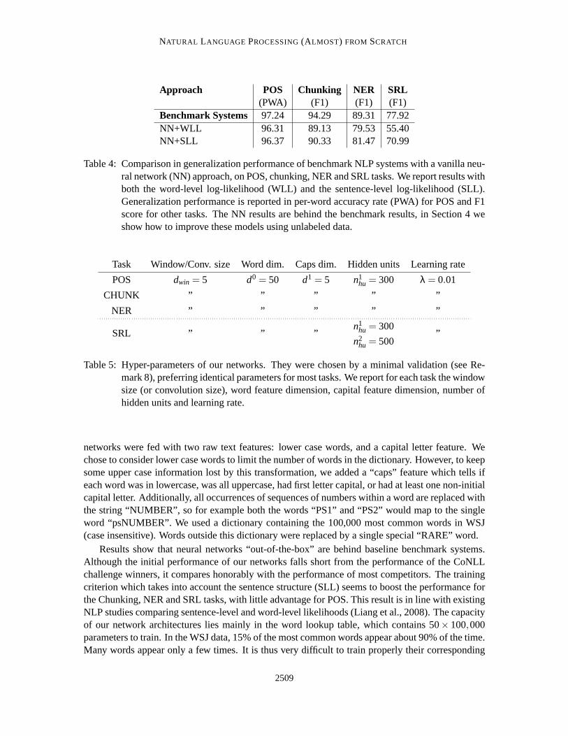
Approach POS Chunking NER SRL(PWA) (F1) (F1) (F1)
Benchmark Systems 97.24 94.29 89.31 77.92NN+WLL 96.31 89.13 79.53 55.40NN+SLL 96.37 90.33 81.47 70.99
Table 4: Comparison in generalization performance of benchmark NLP systems with a vanilla neu-ral network (NN) approach, on POS, chunking, NER and SRL tasks. We report results withboth the word-level log-likelihood (WLL) and the sentence-level log-likelihood (SLL).Generalization performance is reported in per-word accuracy rate (PWA) for POS and F1score for other tasks. The NN results are behind the benchmark results,in Section 4 weshow how to improve these models using unlabeled data.
Task Window/Conv. size Word dim. Caps dim. Hidden units Learning rate
POS dwin = 5 d0 = 50 d1 = 5 n1hu = 300 λ = 0.01
CHUNK ” ” ” ” ”
NER ” ” ” ” ”
SRL ” ” ”n1
hu = 300
n2hu = 500
”
Table 5: Hyper-parameters of our networks. They were chosen by a minimal validation (see Re-mark 8), preferring identical parameters for most tasks. We report foreach task the windowsize (or convolution size), word feature dimension, capital feature dimension, number ofhidden units and learning rate.
networks were fed with two raw text features: lower case words, and a capital letter feature. Wechose to consider lower case words to limit the number of words in the dictionary. However, to keepsome upper case information lost by this transformation, we added a “caps”feature which tells ifeach word was in lowercase, was all uppercase, had first letter capital,or had at least one non-initialcapital letter. Additionally, all occurrences of sequences of numbers within a word are replaced withthe string “NUMBER”, so for example both the words “PS1” and “PS2” would map to the singleword “psNUMBER”. We used a dictionary containing the 100,000 most commonwords in WSJ(case insensitive). Words outside this dictionary were replaced by a single special “RARE” word.
Results show that neural networks “out-of-the-box” are behind baseline benchmark systems.Although the initial performance of our networks falls short from the performance of the CoNLLchallenge winners, it compares honorably with the performance of most competitors. The trainingcriterion which takes into account the sentence structure (SLL) seems to boost the performance forthe Chunking, NER and SRL tasks, with little advantage for POS. This result isin line with existingNLP studies comparing sentence-level and word-level likelihoods (Lianget al., 2008). The capacityof our network architectures lies mainly in the word lookup table, which contains 50× 100,000parameters to train. In the WSJ data, 15% of the most common words appear about 90% of the time.Many words appear only a few times. It is thus very difficult to train properly their corresponding
2509
COLLOBERT, WESTON, BOTTOU, KARLEN, KAVUKCUOGLU AND KUKSA
FRANCE JESUS XBOX REDDISH SCRATCHED MEGABITS
454 1973 6909 11724 29869 87025PERSUADE THICKETS DECADENT WIDESCREEN ODD PPA
FAW SAVARY DIVO ANTICA ANCHIETA UDDIN
BLACKSTOCK SYMPATHETIC VERUS SHABBY EMIGRATION BIOLOGICALLY
GIORGI JFK OXIDE AWE MARKING KAYAK
SHAHEED KHWARAZM URBINA THUD HEUER MCLARENS
RUMELIA STATIONERY EPOS OCCUPANT SAMBHAJI GLADWIN
PLANUM ILIAS EGLINTON REVISED WORSHIPPERS CENTRALLY
GOA’ ULD GSNUMBER EDGING LEAVENED RITSUKO INDONESIA
COLLATION OPERATOR FRG PANDIONIDAE LIFELESS MONEO
BACHA W.J. NAMSOS SHIRT MAHAN NILGIRIS
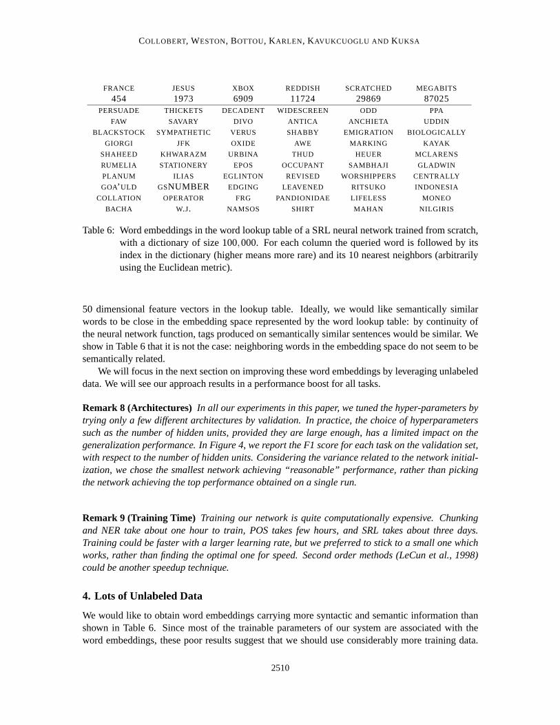
Table 6: Word embeddings in the word lookup table of a SRL neural networktrained from scratch,with a dictionary of size 100,000. For each column the queried word is followed by itsindex in the dictionary (higher means more rare) and its 10 nearest neighbors (arbitrarilyusing the Euclidean metric).
50 dimensional feature vectors in the lookup table. Ideally, we would like semantically similarwords to be close in the embedding space represented by the word lookup table: by continuity ofthe neural network function, tags produced on semantically similar sentences would be similar. Weshow in Table 6 that it is not the case: neighboring words in the embedding space do not seem to besemantically related.
We will focus in the next section on improving these word embeddings by leveraging unlabeleddata. We will see our approach results in a performance boost for all tasks.
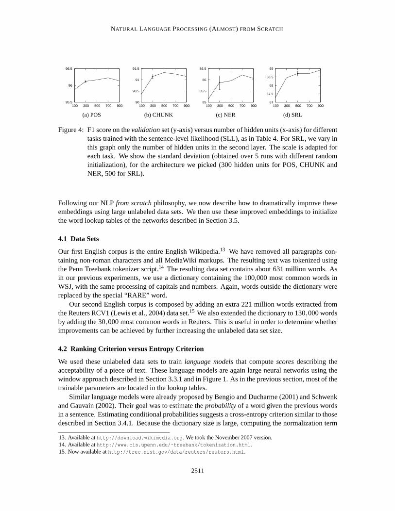
Remark 8 (Architectures) In all our experiments in this paper, we tuned the hyper-parameters bytrying only a few different architectures by validation. In practice, the choice of hyperparameterssuch as the number of hidden units, provided they are large enough, has a limited impact on thegeneralization performance. In Figure 4, we report the F1 score for each task on the validation set,with respect to the number of hidden units. Considering the variance related to the network initial-ization, we chose the smallest network achieving “reasonable” performance, rather than pickingthe network achieving the top performance obtained on a single run.
Remark 9 (Training Time) Training our network is quite computationally expensive. Chunkingand NER take about one hour to train, POS takes few hours, and SRL takesabout three days.Training could be faster with a larger learning rate, but we preferred to stickto a small one whichworks, rather than finding the optimal one for speed. Second order methods (LeCun et al., 1998)could be another speedup technique.
4. Lots of Unlabeled Data
We would like to obtain word embeddings carrying more syntactic and semantic information thanshown in Table 6. Since most of the trainable parameters of our system are associated with theword embeddings, these poor results suggest that we should use considerably more training data.
2510
NATURAL LANGUAGE PROCESSING(ALMOST) FROM SCRATCH
95.5
96
96.5
100 300 500 700 900
(a) POS
90
90.5
91
91.5
100 300 500 700 900
(b) CHUNK
85
85.5
86
86.5
100 300 500 700 900
(c) NER
67
67.5
68
68.5
69
100 300 500 700 900
(d) SRL
Figure 4: F1 score on thevalidationset (y-axis) versus number of hidden units (x-axis) for differenttasks trained with the sentence-level likelihood (SLL), as in Table 4. For SRL, we vary inthis graph only the number of hidden units in the second layer. The scale is adapted foreach task. We show the standard deviation (obtained over 5 runs with different randominitialization), for the architecture we picked (300 hidden units for POS, CHUNK andNER, 500 for SRL).
Following our NLPfrom scratchphilosophy, we now describe how to dramatically improve theseembeddings using large unlabeled data sets. We then use these improved embeddings to initializethe word lookup tables of the networks described in Section 3.5.
4.1 Data Sets
Our first English corpus is the entire English Wikipedia.13 We have removed all paragraphs con-taining non-roman characters and all MediaWiki markups. The resulting text was tokenized usingthe Penn Treebank tokenizer script.14 The resulting data set contains about 631 million words. Asin our previous experiments, we use a dictionary containing the 100,000 mostcommon words inWSJ, with the same processing of capitals and numbers. Again, words outside the dictionary werereplaced by the special “RARE” word.
Our second English corpus is composed by adding an extra 221 million wordsextracted fromthe Reuters RCV1 (Lewis et al., 2004) data set.15 We also extended the dictionary to 130,000 wordsby adding the 30,000 most common words in Reuters. This is useful in order to determine whetherimprovements can be achieved by further increasing the unlabeled data setsize.
4.2 Ranking Criterion versus Entropy Criterion
We used these unlabeled data sets to trainlanguage modelsthat computescoresdescribing theacceptability of a piece of text. These language models are again large neural networks using thewindow approach described in Section 3.3.1 and in Figure 1. As in the previous section, most of thetrainable parameters are located in the lookup tables.
Similar language models were already proposed by Bengio and Ducharme (2001) and Schwenkand Gauvain (2002). Their goal was to estimate theprobability of a word given the previous wordsin a sentence. Estimating conditional probabilities suggests a cross-entropycriterion similar to thosedescribed in Section 3.4.1. Because the dictionary size is large, computing thenormalization term
13. Available athttp://download.wikimedia.org . We took the November 2007 version.14. Available athttp://www.cis.upenn.edu/ ˜ treebank/tokenization.html .15. Now available athttp://trec.nist.gov/data/reuters/reuters.html .
2511
COLLOBERT, WESTON, BOTTOU, KARLEN, KAVUKCUOGLU AND KUKSA
can be extremely demanding, and sophisticated approximations are required. More importantly forus, neither work leads to significant word embeddings being reported.
Shannon (1951) has estimated the entropy of the English language between0.6 and 1.3 bits percharacter by asking human subjects to guess upcoming characters. Cover and King (1978) givea lower bound of 1.25 bits per character using a subtle gambling approach.Meanwhile, using asimple word trigram model, Brown et al. (1992b) reach 1.75 bits per character. Teahan and Cleary(1996) obtain entropies as low as 1.46 bits per character using variable length charactern-grams.The human subjects rely of course on all their knowledge of the language and of the world. Can welearn the grammatical structure of the English language and the nature of the world by leveragingthe 0.2 bits per character that separate human subjects from simple n-gram models? Since such taskscertainly require high capacity models, obtaining sufficiently small confidenceintervals on the testset entropy may require prohibitively large training sets.16 The entropy criterion lacks dynamicalrange because its numerical value is largely determined by the most frequentphrases. In order tolearn syntax, rare but legal phrases are no less significant than commonphrases.
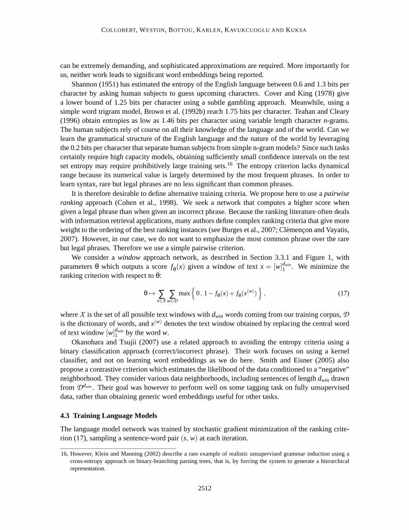
It is therefore desirable to define alternative training criteria. We propose here to use apairwiseranking approach (Cohen et al., 1998). We seek a network that computes a higherscore whengiven a legal phrase than when given an incorrect phrase. Because the ranking literature often dealswith information retrieval applications, many authors define complex ranking criteria that give moreweight to the ordering of the best ranking instances (see Burges et al., 2007; Clemencon and Vayatis,2007). However, in our case, we do not want to emphasize the most commonphrase over the rarebut legal phrases. Therefore we use a simple pairwise criterion.
We consider awindow approach network, as described in Section 3.3.1 and Figure 1, withparametersθ which outputs a scorefθ(x) given a window of textx = [w]dwin
1 . We minimize theranking criterion with respect toθ:
θ 7→ ∑x∈X
∑w∈D
max{
0, 1− fθ(x)+ fθ(x(w))
}
, (17)
whereX is the set of all possible text windows withdwin words coming from our training corpus,Dis the dictionary of words, andx(w) denotes the text window obtained by replacing the central wordof text window[w]dwin
1 by the wordw.Okanohara and Tsujii (2007) use a related approach to avoiding the entropy criteria using a
binary classification approach (correct/incorrect phrase). Their work focuses on using a kernelclassifier, and not on learning word embeddings as we do here. Smith and Eisner (2005) alsopropose a contrastive criterion which estimates the likelihood of the data conditioned to a “negative”neighborhood. They consider various data neighborhoods, includingsentences of lengthdwin drawnfrom Ddwin. Their goal was however to perform well on some tagging task on fully unsuperviseddata, rather than obtaining generic word embeddings useful for other tasks.
4.3 Training Language Models
The language model network was trained by stochastic gradient minimization ofthe ranking crite-rion (17), sampling a sentence-word pair(s, w) at each iteration.
16. However, Klein and Manning (2002) describe a rare example of realistic unsupervised grammar induction using across-entropy approach on binary-branching parsing trees, that is, by forcing the system to generate a hierarchicalrepresentation.
2512
NATURAL LANGUAGE PROCESSING(ALMOST) FROM SCRATCH
Since training times for such large scale systems are counted in weeks, it is not feasible totry many combinations of hyperparameters. It also makes sense to speed upthe training time byinitializing new networks with the embeddings computed by earlier networks. In particular, wefound it expedient to train a succession of networks using increasingly large dictionaries, eachnetwork being initialized with the embeddings of the previous network. Successive dictionary sizesand switching times are chosen arbitrarily. Bengio et al. (2009) provides amore detailed discussionof this, the (as yet, poorly understood) “curriculum” process.
For the purposes of model selection we use the process of “breeding”.The idea of breedingis instead of trying a full grid search of possible values (which we did not have enough computingpower for) to search for the parameters in analogy to breeding biologicalcell lines. Within each line,child networks are initialized with the embeddings of their parents and trained onincreasingly richdata sets with sometimes different parameters. That is, suppose we havek processors, which is muchless than the possible set of parameters one would like to try. One choosesk initial parameter choicesfrom the large set, and trains these on thek processors. In our case, possible parameters to adjustare: the learning rateλ, the word embedding dimensionsd, number of hidden unitsn1
hu and inputwindow sizedwin. One then trains each of these models in an online fashion for a certain amountof time (i.e., a few days), and then selects the best ones using the validation set error rate. That is,breeding decisions were made on the basis of the value of the ranking criterion (17) estimated ona validation set composed of one million words held out from the Wikipedia corpus. In the nextbreeding iteration, one then chooses another set ofk parameters from the possible grid of valuesthat permute slightly the most successful candidates from the previous round. As many of theseparameter choices can share weights, we can effectively continue onlinetraining retaining some ofthe learning from the previous iterations.
Very long training times make such strategies necessary for the foreseeable future: if we hadbeen given computers ten times faster, we probably would have found uses for data sets ten timesbigger. However, we should say we believe that although we ended up witha particular choice ofparameters, many other choices are almost equally as good, although perhaps there are others thatare better as we could not do a full grid search.
In the following subsections, we report results obtained with two trained language models. Theresults achieved by these two models are representative of those achieved by networks trained onthe full corpora.
• Language model LM1 has a window sizedwin = 11 and a hidden layer withn1hu = 100 units.
The embedding layers were dimensioned like those of the supervised networks (Table 5).Model LM1 was trained on our first English corpus (Wikipedia) using successive dictionariescomposed of the 5000, 10,000, 30,000, 50,000 and finally 100,000 most common WSJwords. The total training time was about four weeks.
• Language model LM2 has the same dimensions. It was initialized with the embeddings ofLM1, and trained for an additional three weeks on our second English corpus(Wikipedia+Reuters) using a dictionary size of 130,000 words.
4.4 Embeddings
Both networks produce much more appealing word embeddings than in Section3.5. Table 7 showsthe ten nearest neighbors of a few randomly chosen query words for the LM1 model. The syntactic
2513
COLLOBERT, WESTON, BOTTOU, KARLEN, KAVUKCUOGLU AND KUKSA
FRANCE JESUS XBOX REDDISH SCRATCHED MEGABITS
454 1973 6909 11724 29869 87025AUSTRIA GOD AMIGA GREENISH NAILED OCTETS
BELGIUM SATI PLAYSTATION BLUISH SMASHED MB/SGERMANY CHRIST MSX PINKISH PUNCHED BIT/S
ITALY SATAN IPOD PURPLISH POPPED BAUD
GREECE KALI SEGA BROWNISH CRIMPED CARATS
SWEDEN INDRA PSNUMBER GREYISH SCRAPED KBIT/SNORWAY VISHNU HD GRAYISH SCREWED MEGAHERTZ
EUROPE ANANDA DREAMCAST WHITISH SECTIONED MEGAPIXELS
HUNGARY PARVATI GEFORCE SILVERY SLASHED GBIT/SSWITZERLAND GRACE CAPCOM YELLOWISH RIPPED AMPERES
Table 7: Word embeddings in the word lookup table of the language model neural network LM1trained with a dictionary of size 100,000. For each column the queried word is followedby its index in the dictionary (higher means more rare) and its 10 nearest neighbors (usingthe Euclidean metric, which was chosen arbitrarily).
and semantic properties of the neighbors are clearly related to those of the query word. Theseresults are far more satisfactory than those reported in Table 7 for embeddings obtained using purelysupervised training of the benchmark NLP tasks.
4.5 Semi-supervised Benchmark Results
Semi-supervised learning has been the object of much attention during the last few years (seeChapelle et al., 2006). Previous semi-supervised approaches for NLPcan be roughly categorized asfollows:
• Ad-hoc approaches such as Rosenfeld and Feldman (2007) for relation extraction.
• Self-training approaches, such as Ueffing et al. (2007) for machine translation, and McCloskyet al. (2006) for parsing. These methods augment the labeled training setwith examples fromthe unlabeled data set using the labels predicted by the model itself. Transductive approaches,such as Joachims (1999) for text classification can be viewed as a refined form of self-training.
• Parameter sharing approaches such as Ando and Zhang (2005); Suzuki and Isozaki (2008).Ando and Zhang propose a multi-task approach where they jointly train modelssharing cer-tain parameters. They train POS and NER models together with a language model(trained on15 million words) consisting of predicting words given the surrounding tokens. Suzuki andIsozaki embed a generative model (Hidden Markov Model) inside a CRF for POS, Chunkingand NER. The generative model is trained on one billion words. These approaches shouldbe seen as a linear counterpart of our work. Using multilayer models vastly expands theparameter sharing opportunities (see Section 5).
Our approach simply consists of initializing the word lookup tables of the supervised networkswith the embeddings computed by the language models. Supervised training is then performed asin Section 3.5. In particular the supervised training stage is free to modify the lookup tables. Thissequential approach is computationally convenient because it separatesthe lengthy training of the
2514
NATURAL LANGUAGE PROCESSING(ALMOST) FROM SCRATCH
Approach POS CHUNK NER SRL(PWA) (F1) (F1) (F1)
Benchmark Systems 97.24 94.29 89.31 77.92NN+WLL 96.31 89.13 79.53 55.40NN+SLL 96.37 90.33 81.47 70.99NN+WLL+LM1 97.05 91.91 85.68 58.18NN+SLL+LM1 97.10 93.65 87.58 73.84NN+WLL+LM2 97.14 92.04 86.96 58.34NN+SLL+LM2 97.20 93.63 88.67 74.15
Table 8: Comparison in generalization performance of benchmark NLP systems with our (NN) ap-proach on POS, chunking, NER and SRL tasks. We report results with both the word-levellog-likelihood (WLL) and the sentence-level log-likelihood (SLL). We report with (LMn)performance of the networks trained from the language model embeddings(Table 7). Gen-eralization performance is reported in per-word accuracy (PWA) for POS and F1 score forother tasks.
language models from the relatively fast training of the supervised networks. Once the languagemodels are trained, we can perform multiple experiments on the supervised networks in a rela-tively short time. Note that our procedure is clearly linked to the (semi-supervised) deep learningprocedures of Hinton et al. (2006), Bengio et al. (2007) and Weston et al. (2008).
Table 8 clearly shows that this simple initialization significantly boosts the generalization per-formance of the supervised networks for each task. It is worth mentioningthe larger languagemodel led to even better performance. This suggests that we could still take advantage of evenbigger unlabeled data sets.
4.6 Ranking and Language
There is a large agreement in the NLP community that syntax is a necessary prerequisite for se-mantic role labeling (Gildea and Palmer, 2002). This is why state-of-the-art semantic role labelingsystems thoroughly exploit multiple parse trees. The parsers themselves (Charniak, 2000; Collins,1999) contain considerable prior information about syntax (one can think of this as a kind of in-formed pre-processing).
Our system does not use such parse trees because we attempt to learn thisinformation from theunlabeled data set. It is therefore legitimate to question whether our ranking criterion (17) has theconceptual capability to capture such a rich hierarchical information. At first glance, the rankingtask appears unrelated to the induction of probabilistic grammars that underlystandard parsingalgorithms. The lack of hierarchical representation seems a fatal flaw (Chomsky, 1956).
However, ranking is closely related to an alternative description of the language structure:op-erator grammars(Harris, 1968). Instead of directly studying the structure of a sentence, Harrisdefines an algebraic structure on the space of all sentences. Starting from a couple of elementarysentence forms, sentences are described by the successive application of sentence transformationoperators. The sentence structure is revealed as a side effect of the successive transformations.Sentence transformations can also have a semantic interpretation.
2515
COLLOBERT, WESTON, BOTTOU, KARLEN, KAVUKCUOGLU AND KUKSA
In the spirit of structural linguistics, Harris describes procedures to discover sentence trans-formation operators by leveraging the statistical regularities of the language. Such procedures areobviously useful for machine learning approaches. In particular, he proposes a test to decide whethertwo sentences forms are semantically related by a transformation operator. He first defines a rankingcriterion (Harris, 1968, Section 4.1):
“Starting for convenience with very short sentence forms, sayABC, we choose aparticular word choice for all the classes, sayBqCq, except one, in this caseA; for everypair of membersAi , A j of that word class we ask how the sentence formed with oneof the members, that is,AiBqCq compares as to acceptability with the sentence formedwith the other member, that is,A jBqCq.”
Thesegradingsare then used to compare sentence forms:
“It now turns out that, given the gradedn-tuples of words for a particular sentenceform, we can find other sentences forms of the same word classes in which the samen-tuples of words produce the same grading of sentences.”
This is an indication that these two sentence forms exploit common words with the same syntac-tic function and possibly the same meaning. This observation forms the empiricalbasis for theconstruction of operator grammars that describe real-world natural languages such as English.
Therefore there are solid reasons to believe that the ranking criterion (17) has the conceptualpotential to capture strong syntactic and semantic information. On the other hand, the structureof our language models is probably too restrictive for such goals, and our current approach onlyexploits the word embeddings discovered during training.
5. Multi-Task Learning
It is generally accepted that featurestrained for one task can be useful forrelated tasks. This ideawas already exploited in the previous section when certain language model features, namely theword embeddings, were used to initialize the supervised networks.
Multi-task learning (MTL) leverages this idea in a more systematic way. Models for all tasksof interests arejointly trained with an additional linkage between their trainable parameters in thehope of improving the generalization error. This linkage can take the form of a regularizationterm in the joint cost function that biases the models towards common representations. A muchsimpler approach consists in having the modelsshare certain parametersdefined a priori. Multi-task learning has a long history in machine learning and neural networks. Caruana (1997) gives agood overview of these past efforts.
5.1 Joint Decoding versus Joint Training
Multitask approaches do not necessarily involve joint training. For instance, modern speech recog-nition systems use Bayes rule to combine the outputs of an acoustic model trained on speech dataand a language model trained on phonetic or textual corpora (Jelinek, 1976). This joint decodingapproach has been successfully applied to structurally more complex NLP tasks. Sutton and McCal-lum (2005b) obtain improved results by combining the predictions of independently trained CRFmodels using a joint decoding process at test time that requires more sophisticated probabilistic
2516
NATURAL LANGUAGE PROCESSING(ALMOST) FROM SCRATCH
inference techniques. On the other hand, Sutton and McCallum (2005a) obtain results somewhatbelow the state-of-the-art using joint decoding for SRL and syntactic parsing. Musillo and Merlo(2006) also describe a negative result at the same joint task.
Joint decoding invariably works by considering additional probabilistic dependency paths be-tween the models. Therefore it defines an implicit supermodel that describes all the tasks in thesame probabilistic framework. Separately training a submodel only makes sense when the train-ing data blocks these additional dependency paths (in the sense of d-separation, Pearl, 1988). Thisimplies that, without joint training, the additional dependency paths cannot directly involve unob-served variables. Therefore, the natural idea of discovering common internal representations acrosstasks requires joint training.
Joint training is relatively straightforward when the training sets for the individual tasks con-tain the same patterns with different labels. It is then sufficient to train a modelthat computesmultiple outputs for each pattern (Suddarth and Holden, 1991). Using this scheme, Sutton et al.(2007) demonstrate improvements on POS tagging and noun-phrase chunking using jointly trainedCRFs. However the joint labeling requirement is a limitation because such data isnot often avail-able. Miller et al. (2000) achieves performance improvements by jointly training NER, parsing,and relation extraction in a statistical parsing model. The joint labeling requirement problem wasweakened using a predictor to fill in the missing annotations.
Ando and Zhang (2005) propose a setup that works around the joint labeling requirements. Theydefine linear models of the formfi(x) = w⊤i Φ(x)+v⊤i ΘΨ(x) where fi is the classifier for thei-thtask with parameterswi andvi . NotationsΦ(x) andΨ(x) represent engineered features for the pat-ternx. Matrix Θ maps theΨ(x) features into a low dimensional subspace common across all tasks.Each task is trained using its own examples without a joint labeling requirement. The learning pro-cedure alternates the optimization ofwi andvi for each task, and the optimization ofΘ to minimizethe average loss for all examples in all tasks. The authors also consider auxiliary unsupervised tasksfor predicting substructures. They report excellent results on several tasks, including POS and NER.
5.2 Multi-Task Benchmark Results
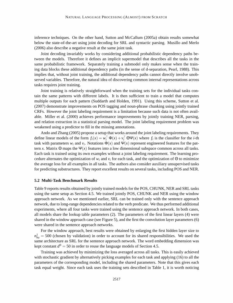
Table 9 reports results obtained by jointly trained models for the POS, CHUNK,NER and SRL tasksusing the same setup as Section 4.5. We trained jointly POS, CHUNK and NER using the windowapproach network. As we mentioned earlier, SRL can be trained only with thesentence approachnetwork, due to long-range dependencies related to the verb predicate.We thus performed additionalexperiments, where all four tasks were trained using the sentence approach network. In both cases,all models share the lookup table parameters (2). The parameters of the first linear layers (4) wereshared in the window approach case (see Figure 5), and the first the convolution layer parameters (6)were shared in the sentence approach networks.
For the window approach, best results were obtained by enlarging the first hidden layer size ton1
hu = 500 (chosen by validation) in order to account for its shared responsibilities. We used thesame architecture as SRL for the sentence approach network. The wordembedding dimension waskept constantd0 = 50 in order to reuse the language models of Section 4.5.
Training was achieved by minimizing the loss averaged across all tasks. Thisis easily achievedwith stochastic gradient by alternatively picking examples for each task andapplying (16) to all theparameters of the corresponding model, including the shared parameters.Note that this gives eachtask equal weight. Since each task uses the training sets described in Table1, it is worth noticing
2517
COLLOBERT, WESTON, BOTTOU, KARLEN, KAVUKCUOGLU AND KUKSA
Lookup Table
Linear
Lookup Table
Linear
HardTanh HardTanh
Linear
Task 1
Linear
Task 2
M2(t1) × · M
2(t2) × ·
xxxxxxxxxxxxxxxxxxxxxxxxxxxxxxxxxxxxxxxxxxxxxxxxxxxxxxxxxxxxxxxxxxxxxxxxxxxxxxxxxxxxxxxxxxxxxxxxxxxxxxxxxxxxxxxxxxxxxxxxxxxxxxxxxxxxxxxxxxxxxxxxxxxxxxxxxxxxxxxxxxxxxxxxxxxxxxxxxxxxLTW 1
.
.
.
LTW K
M1× ·xxxxxxxxxxxxxxxxxxxxxxxxxxxxxxxn1
hu xxxxxxxxxxxxxxxxxxxxxxxxxxxxxxxn1huxxxxxxxxxxxxxxxxxxxxxxxxxxxxxx xxxxxxxxxxxxxxxxxxxxxxxxxxxxxxxxxxxxxxxxxxxxxxxxn2
hu,(t1)= #tags xxxxxxxxxxxxxxxxxxxxxxxn2
hu,(t2)= #tags
Figure 5: Example of multitasking with NN. Task 1 and Task 2 are two tasks trained with thewindow approach architecture presented in Figure 1. Lookup tables as well as the firsthidden layer are shared. The last layer is task specific. The principle is the same withmore than two tasks.
that examples can come from quite different data sets. The generalization performance for eachtask was measured using the traditional testing data specified in Table 1. Fortunately, none of thetraining and test sets overlap across tasks.
It is worth mentioning that MTL can produce a singleunified networkthat performs well forall these tasks using the sentence approach. However this unified network only leads to marginalimprovements over using a separate network for each task: the most important MTL task appears tobe the unsupervised learning of the word embeddings. As explained before, simple computationalconsiderations led us to train the POS, Chunking, and NER tasks using the window approach. Thebaseline results in Table 9 also show that using the sentence approach forthe POS, Chunking, andNER tasks yields no performance improvement (or degradation) over the window approach. Thenext section shows we can leverage known correlations between tasks inmore direct manner.
6. The Temptation
Results so far have been obtained by staying (almost17) true to ourfrom scratchphilosophy. Wehave so far avoided specializing our architecture for any task, disregarding a lot of usefula priori
17. We did some basic preprocessing of the raw input words as described in Section 3.5, hence the “almost” in the title ofthis article. A completely from scratch approach would presumably not know anything about words at all and wouldwork from letters only (or, taken to a further extreme, from speech or optical character recognition, as humans do).
2518
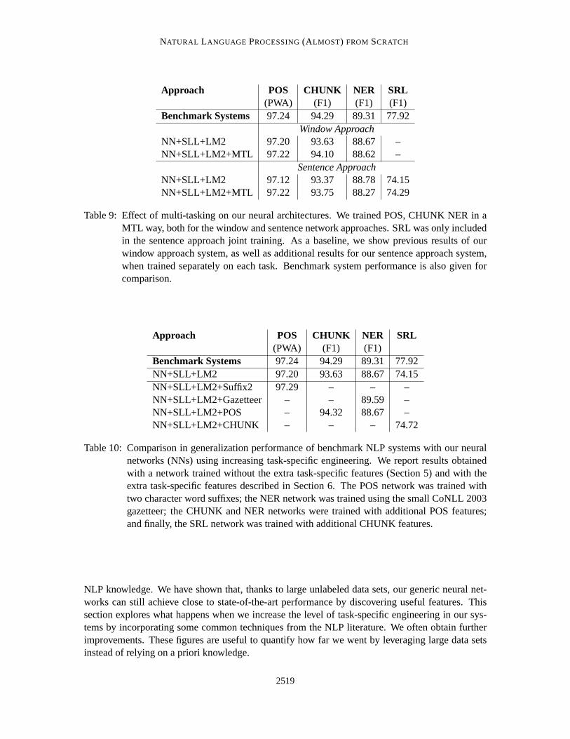
NATURAL LANGUAGE PROCESSING(ALMOST) FROM SCRATCH
Approach POS CHUNK NER SRL(PWA) (F1) (F1) (F1)
Benchmark Systems 97.24 94.29 89.31 77.92Window Approach
NN+SLL+LM2 97.20 93.63 88.67 –NN+SLL+LM2+MTL 97.22 94.10 88.62 –
Sentence ApproachNN+SLL+LM2 97.12 93.37 88.78 74.15NN+SLL+LM2+MTL 97.22 93.75 88.27 74.29
Table 9: Effect of multi-tasking on our neural architectures. We trained POS, CHUNK NER in aMTL way, both for the window and sentence network approaches. SRL was only includedin the sentence approach joint training. As a baseline, we show previous results of ourwindow approach system, as well as additional results for our sentence approach system,when trained separately on each task. Benchmark system performance is also given forcomparison.
Approach POS CHUNK NER SRL(PWA) (F1) (F1)
Benchmark Systems 97.24 94.29 89.31 77.92NN+SLL+LM2 97.20 93.63 88.67 74.15NN+SLL+LM2+Suffix2 97.29 – – –NN+SLL+LM2+Gazetteer – – 89.59 –NN+SLL+LM2+POS – 94.32 88.67 –NN+SLL+LM2+CHUNK – – – 74.72
Table 10: Comparison in generalization performance of benchmark NLP systems with our neuralnetworks (NNs) using increasing task-specific engineering. We report results obtainedwith a network trained without the extra task-specific features (Section 5) and with theextra task-specific features described in Section 6. The POS network was trained withtwo character word suffixes; the NER network was trained using the small CoNLL 2003gazetteer; the CHUNK and NER networks were trained with additional POS features;and finally, the SRL network was trained with additional CHUNK features.
NLP knowledge. We have shown that, thanks to large unlabeled data sets, our generic neural net-works can still achieve close to state-of-the-art performance by discovering useful features. Thissection explores what happens when we increase the level of task-specific engineering in our sys-tems by incorporating some common techniques from the NLP literature. We oftenobtain furtherimprovements. These figures are useful to quantify how far we went by leveraging large data setsinstead of relying on a priori knowledge.
2519
COLLOBERT, WESTON, BOTTOU, KARLEN, KAVUKCUOGLU AND KUKSA
6.1 Suffix Features
Word suffixes in many western languages are strong predictors of the syntactic function of the wordand therefore can benefit the POS system. For instance, Ratnaparkhi (1996) uses inputs representingword suffixes and prefixes up to four characters. We achieve this in thePOS task by adding discreteword features (Section 3.2.1) representing the last two characters of every word. The size of thesuffix dictionary was 455. This led to a small improvement of the POS performance (Table 10,row NN+SLL+LM2+Suffix2). We also tried suffixes obtained with the Porter (1980) stemmer andobtained the same performance as when using two character suffixes.
6.2 Gazetteers
State-of-the-art NER systems often use a large dictionary containing well known named entities(e.g., Florian et al., 2003). We restricted ourselves to the gazetteer provided by the CoNLL chal-lenge, containing 8,000 locations, person names, organizations, and miscellaneous entities. Wetrained a NER network with 4 additional word features indicating (feature “on” or “off”) whetherthe word is found in the gazetteer under one of these four categories. The gazetteer includes notonly words, but also chunks of words. If a sentence chunk is found inthe gazetteer, then all words inthe chunk have their corresponding gazetteer feature turned to “on”. The resulting system displaysa clear performance improvement (Table 10, rowNN+SLL+LM2+Gazetteer), slightly outperformingthe baseline. A plausible explanation of this large boost over the network using only the languagemodel is that gazetteers include word chunks, while we use only the word representation of ourlanguage model. For example, “united” and “bicycle” seen separately arelikely to be non-entities,while “united bicycle” might be an entity, but catching it would require higher level representationsof our language model.
6.3 Cascading
When one considers related tasks, it is reasonable to assume that tags obtained for one task can beuseful for taking decisions in the other tasks. Conventional NLP systems often use features obtainedfrom the output of other preexisting NLP systems. For instance, Shen andSarkar (2005) describe achunking system that uses POS tags as input; Florian et al. (2003) describes a NER system whoseinputs include POS and CHUNK tags, as well as the output of two other NER classifiers. State-of-the-art SRL systems exploit parse trees (Gildea and Palmer, 2002; Punyakanok et al., 2005), relatedto CHUNK tags, and built using POS tags (Charniak, 2000; Collins, 1999).
Table 10 reports results obtained for the CHUNK and NER tasks by adding discrete word fea-tures (Section 3.2.1) representing the POS tags. In order to facilitate comparisons, instead of usingthe more accurate tags from our POS network, we use for each task the POS tags provided by thecorresponding CoNLL challenge. We also report results obtained for the SRL task by adding wordfeatures representing the CHUNK tags (also provided by the CoNLL challenge). We consistentlyobtain moderate improvements.
6.4 Ensembles
Constructing ensembles of classifiers is a proven way to trade computationalefficiency for general-ization performance (Bell et al., 2007). Therefore it is not surprising that many NLP systems achievestate-of-the-art performance by combining the outputs of multiple classifiers. For instance, Kudo
2520
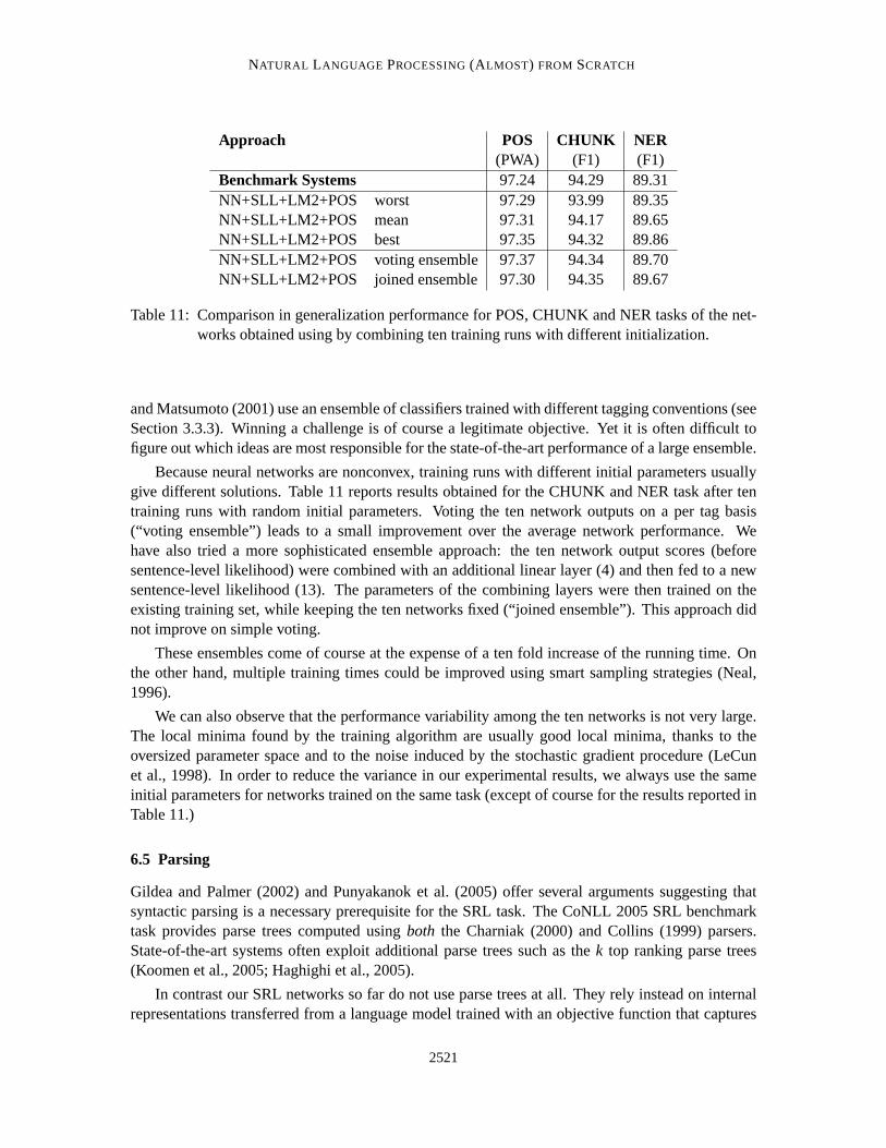
NATURAL LANGUAGE PROCESSING(ALMOST) FROM SCRATCH
Approach POS CHUNK NER(PWA) (F1) (F1)
Benchmark Systems 97.24 94.29 89.31NN+SLL+LM2+POS worst 97.29 93.99 89.35NN+SLL+LM2+POS mean 97.31 94.17 89.65NN+SLL+LM2+POS best 97.35 94.32 89.86NN+SLL+LM2+POS voting ensemble 97.37 94.34 89.70NN+SLL+LM2+POS joined ensemble 97.30 94.35 89.67
Table 11: Comparison in generalization performance for POS, CHUNK andNER tasks of the net-works obtained using by combining ten training runs with different initialization.
and Matsumoto (2001) use an ensemble of classifiers trained with differenttagging conventions (seeSection 3.3.3). Winning a challenge is of course a legitimate objective. Yet it is often difficult tofigure out which ideas are most responsible for the state-of-the-art performance of a large ensemble.
Because neural networks are nonconvex, training runs with different initial parameters usuallygive different solutions. Table 11 reports results obtained for the CHUNK and NER task after tentraining runs with random initial parameters. Voting the ten network outputs on aper tag basis(“voting ensemble”) leads to a small improvement over the average network performance. Wehave also tried a more sophisticated ensemble approach: the ten network output scores (beforesentence-level likelihood) were combined with an additional linear layer (4)and then fed to a newsentence-level likelihood (13). The parameters of the combining layers were then trained on theexisting training set, while keeping the ten networks fixed (“joined ensemble”). This approach didnot improve on simple voting.
These ensembles come of course at the expense of a ten fold increase ofthe running time. Onthe other hand, multiple training times could be improved using smart sampling strategies (Neal,1996).
We can also observe that the performance variability among the ten networksis not very large.The local minima found by the training algorithm are usually good local minima, thanks to theoversized parameter space and to the noise induced by the stochastic gradient procedure (LeCunet al., 1998). In order to reduce the variance in our experimental results, we always use the sameinitial parameters for networks trained on the same task (except of coursefor the results reported inTable 11.)
6.5 Parsing
Gildea and Palmer (2002) and Punyakanok et al. (2005) offer several arguments suggesting thatsyntactic parsing is a necessary prerequisite for the SRL task. The CoNLL 2005 SRL benchmarktask provides parse trees computed usingboth the Charniak (2000) and Collins (1999) parsers.State-of-the-art systems often exploit additional parse trees such as thek top ranking parse trees(Koomen et al., 2005; Haghighi et al., 2005).
In contrast our SRL networks so far do not use parse trees at all. They rely instead on internalrepresentations transferred from a language model trained with an objective function that captures
2521
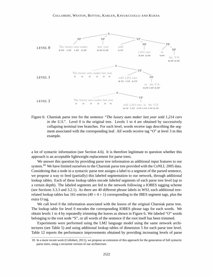
COLLOBERT, WESTON, BOTTOU, KARLEN, KAVUKCUOGLU AND KUKSA
LEVEL 0
S
NP
The luxury auto maker
b-np i-np i-np e-np
NP
last year
b-np e-np
VP
sold
s-vp
NP
1,214 cars
b-np e-np
PP
in
s-pp
NP
the U.S.
b-np e-np
LEVEL 1
S
The luxury auto maker last year
o o o o o o
VP
sold 1,214 cars
b-vp i-vp e-vp
PP
in the U.S.
b-pp i-pp e-pp
LEVEL 2
S
The luxury auto maker last year
o o o o o o
VP
sold 1,214 cars in the U.S.
b-vp i-vp i-vp i-vp i-vp e-vp
Figure 6: Charniak parse tree for the sentence“The luxury auto maker last year sold 1,214 carsin the U.S.”. Level 0 is the original tree. Levels 1 to 4 are obtained by successivelycollapsing terminal tree branches. For each level, words receive tags describing the seg-ment associated with the corresponding leaf. All words receive tag “O” at level 3 in thisexample.
a lot of syntactic information (see Section 4.6). It is therefore legitimate to question whether thisapproach is an acceptable lightweight replacement for parse trees.
We answer this question by providing parse tree information as additional input features to oursystem.18 We have limited ourselves to the Charniak parse tree provided with the CoNLL 2005 data.Considering that a node in a syntactic parse tree assigns a label to a segment of the parsed sentence,we propose a way to feed (partially) this labeled segmentation to our network,through additionallookup tables. Each of these lookup tables encodelabeledsegments of each parse tree level (up toa certain depth). The labeled segments are fed to the network following a IOBES tagging scheme(see Sections 3.3.3 and 3.2.1). As there are 40 different phrase labels inWSJ, each additional tree-related lookup tables has 161 entries (40×4+1) corresponding to the IBES segment tags, plus theextra O tag.
We call level 0 the information associated with the leaves of the original Charniak parse tree.The lookup table for level 0 encodes the corresponding IOBES phrasetags for each words. Weobtain levels 1 to 4 by repeatedly trimming the leaves as shown in Figure 6. We labeled “O” wordsbelonging to the root node “S”, or all words of the sentence if the root itself has been trimmed.
Experiments were performed using the LM2 language model using the same network archi-tectures (see Table 5) and using additional lookup tables of dimension 5 foreach parse tree level.Table 12 reports the performance improvements obtained by providing increasing levels of parse
18. In a more recent work (Collobert, 2011), we propose an extension of this approach for the generation of full syntacticparse trees, using a recurrent version of our architecture.
2522
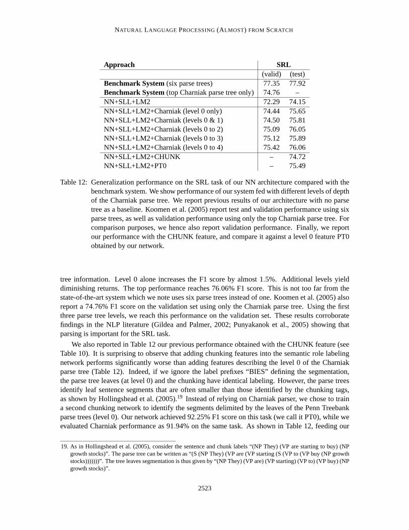
NATURAL LANGUAGE PROCESSING(ALMOST) FROM SCRATCH
Approach SRL(valid) (test)
Benchmark System(six parse trees) 77.35 77.92Benchmark System(top Charniak parse tree only) 74.76 –NN+SLL+LM2 72.29 74.15NN+SLL+LM2+Charniak (level 0 only) 74.44 75.65NN+SLL+LM2+Charniak (levels 0 & 1) 74.50 75.81NN+SLL+LM2+Charniak (levels 0 to 2) 75.09 76.05NN+SLL+LM2+Charniak (levels 0 to 3) 75.12 75.89NN+SLL+LM2+Charniak (levels 0 to 4) 75.42 76.06NN+SLL+LM2+CHUNK – 74.72NN+SLL+LM2+PT0 – 75.49
Table 12: Generalization performance on the SRL task of our NN architecture compared with thebenchmark system. We show performance of our system fed with different levels of depthof the Charniak parse tree. We report previous results of our architecture with no parsetree as a baseline. Koomen et al. (2005) report test and validation performance using sixparse trees, as well as validation performance using only the top Charniakparse tree. Forcomparison purposes, we hence also report validation performance. Finally, we reportour performance with the CHUNK feature, and compare it against a level 0feature PT0obtained by our network.
tree information. Level 0 alone increases the F1 score by almost 1.5%. Additional levels yielddiminishing returns. The top performance reaches 76.06% F1 score. This is not too far from thestate-of-the-art system which we note uses six parse trees instead of one. Koomen et al. (2005) alsoreport a 74.76% F1 score on the validation set using only the Charniak parse tree. Using the firstthree parse tree levels, we reach this performance on the validation set. These results corroboratefindings in the NLP literature (Gildea and Palmer, 2002; Punyakanok et al., 2005) showing thatparsing is important for the SRL task.
We also reported in Table 12 our previous performance obtained with the CHUNK feature (seeTable 10). It is surprising to observe that adding chunking features intothe semantic role labelingnetwork performs significantly worse than adding features describing thelevel 0 of the Charniakparse tree (Table 12). Indeed, if we ignore the label prefixes “BIES”defining the segmentation,the parse tree leaves (at level 0) and the chunking have identical labeling. However, the parse treesidentify leaf sentence segments that are often smaller than those identified by the chunking tags,as shown by Hollingshead et al. (2005).19 Instead of relying on Charniak parser, we chose to traina second chunking network to identify the segments delimited by the leaves of thePenn Treebankparse trees (level 0). Our network achieved 92.25% F1 score on this task (we call it PT0), while weevaluated Charniak performance as 91.94% on the same task. As shown in Table 12, feeding our
19. As in Hollingshead et al. (2005), consider the sentence and chunk labels “(NP They) (VP are starting to buy) (NPgrowth stocks)”. The parse tree can be written as “(S (NP They) (VP are (VP starting (S (VP to (VP buy (NP growthstocks)))))))”. The tree leaves segmentation is thus given by “(NP They) (VP are) (VP starting) (VP to) (VP buy) (NPgrowth stocks)”.
2523
COLLOBERT, WESTON, BOTTOU, KARLEN, KAVUKCUOGLU AND KUKSA
own PT0 prediction into the SRL system gives similar performance to using Charniak predictions,and is consistently better than the CHUNK feature.
6.6 Word Representations
We have described how we induced useful word embeddings by applyingour architecture to alanguage modeling task trained using a large amount of unlabeled text data. These embeddingsimprove the generalization performance on all tasks (Section 4.) The literature describes other waysto induce word representations. Mnih and Hinton (2007) proposed a related language model ap-proach inspired from Restricted Boltzmann Machines. However, word representations are perhapsmore commonly inferred fromn-gram language modeling rather than purely continuous languagemodels. One popular approach is the Brown clustering algorithm (Brown etal., 1992a), whichbuilds hierarchical word clusters by maximizing the bigram’s mutual information.The inducedword representation has been used with success in a wide variety of NLP tasks, including POS(Schutze, 1995), NER (Miller et al., 2004; Ratinov and Roth, 2009), or parsing (Koo et al., 2008).Other related approaches exist, like phrase clustering (Lin and Wu, 2009) which has been shown towork well for NER. Finally, Huang and Yates (2009) have recently proposed a smoothed languagemodeling approach based on a Hidden Markov Model, with success on POSand Chunking tasks.
While a comparison of all these word representations is beyond the scope of this paper, it israther fair to question the quality of our word embeddings compared to a popular NLP approach.In this section, we report a comparison of our word embeddings against Brown clusters, when usedas features into our neural network architecture. We report as baseline previous results where ourword embeddings arefine-tunedfor each task. We also report performance when our embeddingsare kept fixed during task-specific training. Sinceconvexmachine learning algorithms are commonpractice in NLP, we finally report performances for the convex versionof our architecture.
For the convex experiments, we considered the linear version of our neural networks (instead ofhaving several linear layers interleaved with a non-linearity). While we always picked the sentenceapproach for SRL, we had to consider the window approach in this particular convex setup, as thesentence approach network (see Figure 2) includes a Max layer. Having only one linear layer in ourneural network is not enough to make our architecture convex: all lookup-tables (for each discretefeature) must also befixed. The word-lookup table is simply fixed to the embeddings obtained fromour language model LM2. All other discrete feature lookup-tables (caps, POS, Brown Clusters...)are fixed to a standardsparserepresentation. Using the notation introduced in Section 3.2.1, ifLTWk
is the lookup-table of thekth discrete feature, we haveWk ∈R|Dk|×|Dk| and the representation of the
discrete inputw is obtained with:
LTWk(w) = 〈Wk〉1w =
(
0, · · ·0, 1at indexw
, 0, · · · 0
)T
. (18)
Training our architecture in this convex setup with the sentence-level likelihood (13) correspondsto training a CRF. In that respect, these convex experiments show the performance of our wordembeddings in a classical NLP framework.
Following the Ratinov and Roth (2009) and Koo et al. (2008) setups, we generated 1,000 Brownclusters using the implementation20 from Liang (2005). To make the comparison fair, the clusterswere first induced on the concatenation of Wikipedia and Reuters data sets, as we did in Section 4
20. Available athttp://www.eecs.berkeley.edu/ ˜ pliang/software .
2524
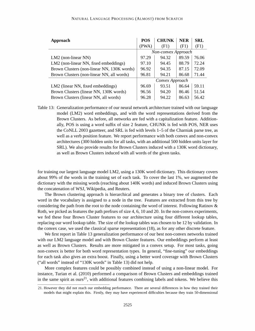
NATURAL LANGUAGE PROCESSING(ALMOST) FROM SCRATCH
Approach POS CHUNK NER SRL(PWA) (F1) (F1) (F1)
Non-convex ApproachLM2 (non-linear NN) 97.29 94.32 89.59 76.06LM2 (non-linear NN, fixed embeddings) 97.10 94.45 88.79 72.24Brown Clusters (non-linear NN, 130K words) 96.92 94.35 87.15 72.09Brown Clusters (non-linear NN, all words) 96.81 94.21 86.68 71.44
Convex ApproachLM2 (linear NN, fixed embeddings) 96.69 93.51 86.64 59.11Brown Clusters (linear NN, 130K words) 96.56 94.20 86.46 51.54Brown Clusters (linear NN, all words) 96.28 94.22 86.63 56.42
Table 13: Generalization performance of our neural network architecture trained with our languagemodel (LM2) word embeddings, and with the word representations derived from theBrown Clusters. As before, all networks are fed with a capitalization feature. Addition-ally, POS is using a word suffix of size 2 feature, CHUNK is fed with POS, NER usesthe CoNLL 2003 gazetteer, and SRL is fed with levels 1–5 of the Charniak parse tree, aswell as a verb position feature. We report performance with both convexand non-convexarchitectures (300 hidden units for all tasks, with an additional 500 hiddenunits layer forSRL). We also provide results for Brown Clusters induced with a 130K word dictionary,as well as Brown Clusters induced with all words of the given tasks.
for training our largest language model LM2, using a 130K word dictionary. This dictionary coversabout 99% of the words in the training set of each task. To cover the last 1%, we augmented thedictionary with the missing words (reaching about 140K words) and inducedBrown Clusters usingthe concatenation of WSJ, Wikipedia, and Reuters.
The Brown clustering approach is hierarchical and generates a binarytree of clusters. Eachword in the vocabulary is assigned to a node in the tree. Features are extracted from this tree byconsidering the path from the root to the node containing the word of interest. Following Ratinov &Roth, we picked as features the path prefixes of size 4, 6, 10 and 20. Inthe non-convex experiments,we fed these four Brown Cluster features to our architecture using fourdifferent lookup tables,replacing our word lookup table. The size of the lookup tables was chosento be 12 by validation. Inthe convex case, we used the classical sparse representation (18), as for any other discrete feature.
We first report in Table 13 generalization performance of our best non-convex networks trainedwith our LM2 language model and with Brown Cluster features. Our embeddings perform at leastas well as Brown Clusters. Results are more mitigated in a convex setup. For most tasks, goingnon-convex is better for both word representation types. In general, “fine-tuning” our embeddingsfor each task also gives an extra boost. Finally, using a better word coverage with Brown Clusters(“all words” instead of “130K words” in Table 13) did not help.
More complex features could be possibly combined instead of using a non-linear model. Forinstance, Turian et al. (2010) performed a comparison of Brown Clusters and embeddings trainedin the same spirit as ours21, with additional features combining labels and tokens. We believe this
21. However they did not reach our embedding performance. Thereare several differences in how they trained theirmodels that might explain this. Firstly, they may have experienced difficulties because they train 50-dimensional
2525
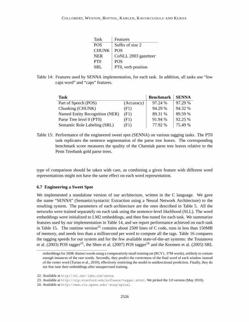
COLLOBERT, WESTON, BOTTOU, KARLEN, KAVUKCUOGLU AND KUKSA
Task FeaturesPOS Suffix of size 2CHUNK POSNER CoNLL 2003 gazetteerPT0 POSSRL PT0, verb position
Table 14: Features used by SENNA implementation, for each task. In addition, all tasks use “lowcaps word” and “caps” features.
Task Benchmark SENNAPart of Speech (POS) (Accuracy) 97.24 % 97.29 %Chunking (CHUNK) (F1) 94.29 % 94.32 %Named Entity Recognition (NER) (F1) 89.31 % 89.59 %Parse Tree level 0 (PT0) (F1) 91.94 % 92.25 %Semantic Role Labeling (SRL) (F1) 77.92 % 75.49 %
Table 15: Performance of the engineered sweet spot (SENNA) on various tagging tasks. The PT0task replicates the sentence segmentation of the parse tree leaves. The correspondingbenchmark score measures the quality of the Charniak parse tree leaves relative to thePenn Treebank gold parse trees.
type of comparison should be taken with care, as combining a given featurewith different wordrepresentations might not have the same effect on each word representation.
6.7 Engineering a Sweet Spot
We implemented a standalone version of our architecture, written in the C language. We gavethe name “SENNA” (Semantic/syntactic Extraction using a Neural Network Architecture) to theresulting system. The parameters of each architecture are the ones described in Table 5. All thenetworks were trained separately on each task using the sentence-levellikelihood (SLL). The wordembeddings were initialized to LM2 embeddings, and then fine-tuned for eachtask. We summarizefeatures used by our implementation in Table 14, and we report performanceachieved on each taskin Table 15. The runtime version22 contains about 2500 lines of C code, runs in less than 150MBof memory, and needs less than a millisecond per word to compute all the tags. Table 16 comparesthe tagging speeds for our system and for the few available state-of-the-art systems: the Toutanovaet al. (2003) POS tagger23, the Shen et al. (2007) POS tagger24 and the Koomen et al. (2005) SRL
embeddings for 269K distinct words using a comparatively small trainingset (RCV1, 37M words), unlikely to containenough instances of the rare words. Secondly, they predict the correctness of the final word of each window insteadof the center word (Turian et al., 2010), effectively restricting the model to unidirectional prediction. Finally, they donot fine tune their embeddings after unsupervised training.
22. Available athttp://ml.nec-labs.com/senna .23. Available athttp://nlp.stanford.edu/software/tagger.shtml . We picked the 3.0 version (May 2010).24. Available athttp://www.cis.upenn.edu/ ˜ xtag/spinal .
2526
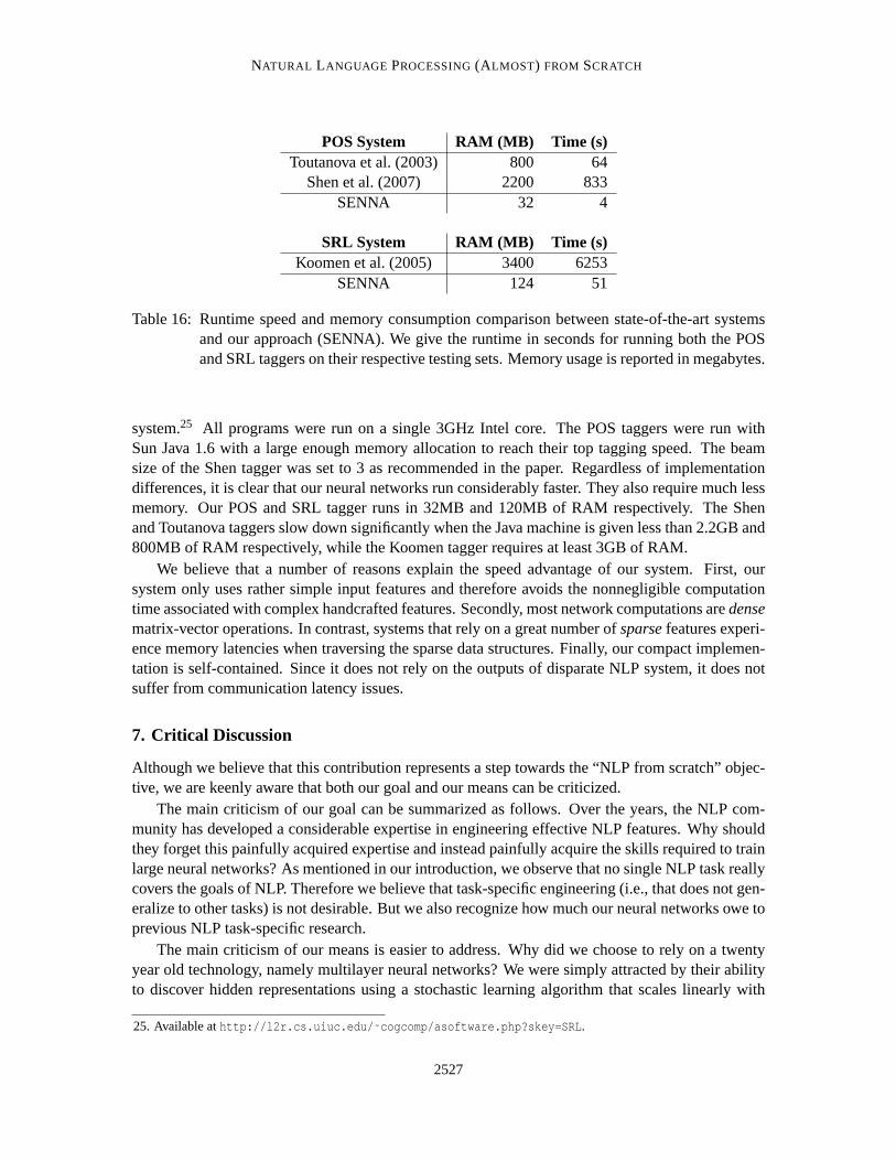
NATURAL LANGUAGE PROCESSING(ALMOST) FROM SCRATCH
POS System RAM (MB) Time (s)Toutanova et al. (2003) 800 64
Shen et al. (2007) 2200 833SENNA 32 4
SRL System RAM (MB) Time (s)Koomen et al. (2005) 3400 6253
SENNA 124 51
Table 16: Runtime speed and memory consumption comparison between state-of-the-art systemsand our approach (SENNA). We give the runtime in seconds for runningboth the POSand SRL taggers on their respective testing sets. Memory usage is reported in megabytes.
system.25 All programs were run on a single 3GHz Intel core. The POS taggers were run withSun Java 1.6 with a large enough memory allocation to reach their top tagging speed. The beamsize of the Shen tagger was set to 3 as recommended in the paper. Regardless of implementationdifferences, it is clear that our neural networks run considerably faster. They also require much lessmemory. Our POS and SRL tagger runs in 32MB and 120MB of RAM respectively. The Shenand Toutanova taggers slow down significantly when the Java machine is given less than 2.2GB and800MB of RAM respectively, while the Koomen tagger requires at least 3GB of RAM.
We believe that a number of reasons explain the speed advantage of our system. First, oursystem only uses rather simple input features and therefore avoids the nonnegligible computationtime associated with complex handcrafted features. Secondly, most networkcomputations aredensematrix-vector operations. In contrast, systems that rely on a great numberof sparsefeatures experi-ence memory latencies when traversing the sparse data structures. Finally,our compact implemen-tation is self-contained. Since it does not rely on the outputs of disparate NLP system, it does notsuffer from communication latency issues.
7. Critical Discussion
Although we believe that this contribution represents a step towards the “NLPfrom scratch” objec-tive, we are keenly aware that both our goal and our means can be criticized.
The main criticism of our goal can be summarized as follows. Over the years,the NLP com-munity has developed a considerable expertise in engineering effective NLP features. Why shouldthey forget this painfully acquired expertise and instead painfully acquirethe skills required to trainlarge neural networks? As mentioned in our introduction, we observe thatno single NLP task reallycovers the goals of NLP. Therefore we believe that task-specific engineering (i.e., that does not gen-eralize to other tasks) is not desirable. But we also recognize how much our neural networks owe toprevious NLP task-specific research.
The main criticism of our means is easier to address. Why did we choose to relyon a twentyyear old technology, namely multilayer neural networks? We were simply attracted by their abilityto discover hidden representations using a stochastic learning algorithm that scales linearly with
25. Available athttp://l2r.cs.uiuc.edu/ ˜ cogcomp/asoftware.php?skey=SRL .
2527
COLLOBERT, WESTON, BOTTOU, KARLEN, KAVUKCUOGLU AND KUKSA
the number of examples. Most of the neural network technology necessary for our work has beendescribed ten years ago (e.g., Le Cun et al., 1998). However, if we haddecided ten years ago to trainthe language model network LM2 using a vintage computer, training would onlybe nearing com-pletion today. Training algorithms that scale linearly are most able to benefit from such tremendousprogress in computer hardware.
8. Conclusion
We have presented a multilayer neural network architecture that can handle a number of NLP taskswith both speed and accuracy. The design of this system was determined byour desire to avoidtask-specific engineering as much as possible. Instead we rely on large unlabeled data sets and letthe training algorithm discover internal representations that prove useful for all the tasks of interest.Using this strong basis, we have engineered a fast and efficient “all purpose” NLP tagger that wehope will prove useful to the community.
Acknowledgments
We acknowledge the persistent support of NEC for this research effort. We thank Yoshua Bengio,Samy Bengio, Eric Cosatto, Vincent Etter, Hans-Peter Graf, Ralph Grishman, and Vladimir Vapnikfor their useful feedback and comments.
Appendix A. Neural Network Gradients
We consider a neural networkfθ(·), with parametersθ. We maximize the likelihood (8), or minimizeranking criterion (17), with respect to the parametersθ, using stochastic gradient. By negating thelikelihood, we now assume it all corresponds to minimize a costC( fθ(·)), with respect toθ.
Following the classical “back-propagation” derivations (LeCun, 1985;Rumelhart et al., 1986)and the modular approach shown in Bottou (1991), any feed-forward neural network withL layers,like the ones shown in Figure 1 and Figure 2, can be seen as a composition of functions f l
θ(·),corresponding to each layerl :
fθ(·) = f Lθ ( f L−1
θ (. . . f 1θ (·) . . .))
Partitioning the parameters of the network with respect to each layers 1≤ l ≤ L, we write:
θ = (θ1, . . . , θl , . . . , θL) .
We are now interested in computing the gradients of the cost with respect to each θl . Applying thechain rule (generalized to vectors) we obtain the classical backpropagation recursion:
∂C∂θl =
∂ f lθ
∂θl
∂C
∂ f lθ
(19)
∂C
∂ f l−1θ
=∂ f l
θ
∂ f l−1θ
∂C
∂ f lθ. (20)
In other words, we first initialize the recursion by computing the gradient ofthe cost with respect tothe last layer output∂C/∂ f L
θ . Then each layerl computes the gradient respect to its own parameters
2528
NATURAL LANGUAGE PROCESSING(ALMOST) FROM SCRATCH
with (19), given the gradient coming from its output∂C/∂ f lθ. To perform the backpropagation, it
also computes the gradient with respect to its own inputs, as shown in (20). We now derive thegradients for each layer we used in this paper.
A.1 Lookup Table Layer
Given a matrix of parametersθ1 =W1 and word (or discrete feature) indices[w]T1 , the layer outputsthe matrix:
f lθ([w]
Tl ) =
(
〈W〉1[w]1〈W〉1[w]2
. . . 〈W〉1[w]T
)
.
The gradients of the weights〈W〉1i are given by:
∂C
∂〈W〉1i= ∑{1≤t≤T / [w]t=i}
〈∂C
∂ f lθ〉1i
This sum equals zero if the indexi in the lookup table does not corresponds to a word in the se-quence. In this case, theith column ofW does not need to be updated. As a Lookup Table Layer isalways the first layer, we do not need to compute its gradients with respectto the inputs.
A.2 Linear Layer
Given parametersθl = (Wl ,bl ), and an inputvector fl−1θ the output is given by:
f lθ =Wl f l−1
θ +bl . (21)
The gradients with respect to the parameters are then obtained with:
∂C∂Wl =
[∂C
∂ f lθ
][
f l−1θ
]T
and∂C∂bl =
∂C
∂ f lθ, (22)
and the gradients with respect to the inputs are computed with:
∂C
∂ f l−1θ
=[
Wl]T ∂C
∂ f lθ. (23)
A.3 Convolution Layer
Given a inputmatrix fl−1θ , a Convolution Layerf l
θ(·) applies a Linear Layer operation (21) suc-cessively on each window〈 f l−1
θ 〉dwint (1 ≤ t ≤ T) of size dwin. Using (22), the gradients of the
parameters are thus given by summing over all windows:
∂C∂Wl =
T
∑t=1
[
〈∂C
∂ f lθ〉1t
][
〈 f l−1θ 〉dwin
t
]T
and∂C∂bl =
T
∑t=1
〈∂C
∂ f lθ〉1t .
After initializing the input gradients∂C/∂ f l−1θ to zero, we iterate (23) over all windows for 1≤ t ≤
T, leading theaccumulation26:
〈∂C
∂ f l−1θ〉dwint +=
[
Wl]T
〈∂C
∂ f lθ〉1t .
26. We denote “+=” any accumulation operation.
2529
COLLOBERT, WESTON, BOTTOU, KARLEN, KAVUKCUOGLU AND KUKSA
A.4 Max Layer
Given amatrix fl−1θ , the Max Layer computes
[
f lθ
]
i= max
t
[
〈 f l−1θ 〉1t
]
iandai = argmax
t
[
〈 f l−1θ 〉1t
]
i∀i ,
whereai stores the index of the largest value. We only need to compute the gradient with respect tothe inputs, as this layer has no parameters. The gradient is given by
[
〈∂C
∂ f l−1θ〉1t
]
i
=
{ [
〈 ∂C∂ f l
θ〉1t
]
iif t = ai
0 otherwise.
A.5 HardTanh Layer
Given avector fl−1θ , and the definition of the HardTanh (5) we get
[
∂C
∂ f l−1θ
]
i
=
0 if[
f l−1θ
]
i<−1
[∂C∂ f l
θ
]
iif −1<=
[
f l−1θ
]
i<= 1
0 if[
f l−1θ
]
i> 1
,
if we ignore non-differentiability points.
A.6 Word-Level Log-Likelihood
The network outputs a score[ fθ]i for each tag indexed byi. Following (11), ify is the true tag for agiven example, the stochastic score to minimize can be written as
C( fθ) = logaddj
[ fθ] j − [ fθ]y
Considering the definition of the logadd (10), the gradient with respect tofθ is given by
∂C∂ [ fθ]i
=e[ fθ]i
∑k e[ fθ]k−1i=y ∀i.
A.7 Sentence-Level Log-Likelihood
The network outputs a matrix where each element[
fθ]
i, t gives a score for tagi at wordt. Given a
tag sequence[y]T1 and a input sequence[x]T1 , we maximize the likelihood (13), which correspondsto minimizing the score
C( fθ,A) = logadd∀[ j]T1
s([x]T1 , [ j]T1 , θ)
︸ ︷︷ ︸
Clogadd
−s([x]T1 , [y]T1 , θ) ,
with
s([x]T1 , [y]T1 , θ) =
T
∑t=1
(
[A][y]t−1, [y]t+[ fθ][y]t , t
)
.
2530
NATURAL LANGUAGE PROCESSING(ALMOST) FROM SCRATCH
We first initialize all gradients to zero
∂C
∂[
fθ]
i, t
= 0 ∀i, t and∂C
∂ [A]i, j= 0 ∀i, j .
We thenaccumulategradients over the second part of the cost−s([x]T1 , [y]T1 , θ), which gives:
∂C
∂[
fθ]
[y]t , t
+=1
∂C∂ [A][y]t−1, [y]t
+=1∀t .
We now need to accumulate the gradients over the first part of the cost, thatis Clogadd. We differen-tiateClogadd by applying the chain rule through the recursion (14). First we initialize ourrecursionwith
∂Clogadd
∂δT(i)=
eδT (i)
∑k eδT (k)∀i .
We then compute iteratively:
∂Clogadd
∂δt−1(i)= ∑
j
∂Clogadd
∂δt( j)eδt−1(i)+[A]i, j
∑k eδt−1(k)+[A]k, j,
where at each stept of the recursion we accumulate of the gradients with respect to the inputsfθ,and the transition scores[A]i, j :
∂C
∂[
fθ]
i, t
+=∂Clogadd
∂δt(i)∂δt(i)
∂[
fθ]
i, t
=∂Clogadd
∂δt(i)
∂C∂ [A]i, j
+=∂Clogadd
∂δt( j)∂δt( j)∂ [A]i, j
=∂Clogadd
∂δt( j)eδt−1(i)+[A]i, j
∑k eδt−1(k)+[A]k, j.
A.8 Ranking Criterion
We use the ranking criterion (17) for training our language model. In this case, given a “positive”examplex and a “negative” examplex(w), we want to minimize:
C( fθ(x), fθ(xw)) = max
{
0, 1− fθ(x)+ fθ(x(w))
}
.
Ignoring the non-differentiability ofmax(0, ·) in zero, the gradient is simply given by:
( ∂C∂ fθ(x)
∂C∂ fθ(xw)
)
=
(−1
1
)
if 1− fθ(x)+ fθ(x(w))> 0(
0
0
)
otherwise.
2531
COLLOBERT, WESTON, BOTTOU, KARLEN, KAVUKCUOGLU AND KUKSA
References
R. K. Ando and T. Zhang. A framework for learning predictive structures from multiple tasks andunlabeled data.Journal of Machine Learning Research (JMLR), 6:1817–1953, 2005.
R. M. Bell, Y. Koren, and C. Volinsky. The BellKor solution to the Netflix Prize. Technical report,AT&T Labs, 2007.http://www.research.att.com/ ˜ volinsky/netflix .
Y. Bengio and R. Ducharme. A neural probabilistic language model. InAdvances in Neural Infor-mation Processing Systems (NIPS 13), 2001.
Y. Bengio, P. Lamblin, D. Popovici, and H. Larochelle. Greedy layer-wise training of deep networks.In Advances in Neural Information Processing Systems (NIPS 19), 2007.
Y. Bengio, J. Louradour, R. Collobert, and J. Weston. Curriculum learning. In International Con-ference on Machine Learning (ICML), 2009.
L. Bottou. Stochastic gradient learning in neural networks. InProceedings of Neuro-Nımes. EC2,1991.
L. Bottou. Online algorithms and stochastic approximations. In David Saad, editor, Online Learningand Neural Networks. Cambridge University Press, Cambridge, UK, 1998.
L. Bottou and P. Gallinari. A framework for the cooperation of learning algorithms. InAdvances inNeural Information Processing Systems (NIPS 3). 1991.
L. Bottou, Y. LeCun, and Yoshua Bengio. Global training of document processing systems usinggraph transformer networks. InConference on Computer Vision and Pattern Recognition (CVPR),pages 489–493, 1997.
J. S. Bridle. Probabilistic interpretation of feedforward classification network outputs, with rela-tionships to statistical pattern recognition. In F. Fogelman Soulie and J. Herault, editors,Neu-rocomputing: Algorithms, Architectures and Applications, pages 227–236. NATO ASI Series,1990.
P. F. Brown, P. V. deSouza, R. L. Mercer, V. J. D. Pietra, and J C. Lai. Class-based n-gram modelsof natural language.Computational Linguistics, 18(4):467–479, 1992a.
P. F. Brown, V. J. Della Pietra, R. L. Mercer, S. A. Della Pietra, and J. C. Lai. An estimate of anupper bound for the entropy of english.Computational Linguistics, 18(1):31–41, 1992b.
C. J. C. Burges, R. Ragno, and Quoc Viet Le. Learning to rank with nonsmooth cost functions. InAdvances in Neural Information Processing Systems (NIPS 19), pages 193–200. 2007.
R. Caruana. Multitask Learning.Machine Learning, 28(1):41–75, 1997.
O. Chapelle, B. Schlkopf, and A. Zien.Semi-Supervised Learning. Adaptive computation andmachine learning. MIT Press, Cambridge, Mass., USA, September 2006.
E. Charniak. A maximum-entropy-inspired parser. InConference of the North American Chapter ofthe Association for Computational Linguistics & Human Language Technologies (NAACL-HLT),pages 132–139, 2000.
2532
NATURAL LANGUAGE PROCESSING(ALMOST) FROM SCRATCH
H. L. Chieu. Named entity recognition with a maximum entropy approach. InConference onNatural Language Learning (CoNLL), pages 160–163, 2003.
N. Chomsky. Three models for the description of language.IRE Transactions on InformationTheory, 2(3):113–124, September 1956.
S. Clemencon and N. Vayatis. Ranking the best instances.Journal of Machine Learning Research(JMLR), 8:2671–2699, 2007.
W. W. Cohen, R. E. Schapire, and Y. Singer. Learning to order things.Journal of Artificial Intelli-gence Research (JAIR), 10:243–270, 1998.
T. Cohn and P. Blunsom. Semantic role labelling with tree conditional random fields. InConferenceon Computational Natural Language (CoNLL), 2005.
M. Collins. Head-Driven Statistical Models for Natural Language Parsing. PhD thesis, Universityof Pennsylvania, 1999.
R. Collobert.Large Scale Machine Learning. PhD thesis, Universite Paris VI, 2004.
R. Collobert. Deep learning for efficient discriminative parsing. InInternational Conference onArtificial Intelligence and Statistics (AISTATS), 2011.
T. Cover and R. King. A convergent gambling estimate of the entropy of english. IEEE Transactionson Information Theory, 24(4):413–421, July 1978.
R. Florian, A. Ittycheriah, H. Jing, and T. Zhang. Named entity recognitionthrough classifiercombination. InConference of the North American Chapter of the Association for ComputationalLinguistics & Human Language Technologies (NAACL-HLT), pages 168–171, 2003.
D. Gildea and D. Jurafsky. Automatic labeling of semantic roles.Computational Linguistics, 28(3):245–288, 2002.
D. Gildea and M. Palmer. The necessity of parsing for predicate argument recognition.Meeting ofthe Association for Computational Linguistics (ACL), pages 239–246, 2002.
J. Gimenez and L. Marquez. SVMTool: A general POS tagger generator based on support vectormachines. InConference on Language Resources and Evaluation (LREC), 2004.
A. Haghighi, K. Toutanova, and C. D. Manning. A joint model for semantic role labeling. InConference on Computational Natural Language Learning (CoNLL), June 2005.
Z. S. Harris.Mathematical Structures of Language. John Wiley & Sons Inc., 1968.
D. Heckerman, D. M. Chickering, C. Meek, R. Rounthwaite, and C. Kadie. Dependency networksfor inference, collaborative filtering, and data visualization.Journal of Machine Learning Re-search (JMLR), 1:49–75, 2001.
G. E. Hinton, S. Osindero, and Y.-W. Teh. A fast learning algorithm for deep belief nets.NeuralComputation, 18(7):1527–1554, July 2006.
2533
COLLOBERT, WESTON, BOTTOU, KARLEN, KAVUKCUOGLU AND KUKSA
K. Hollingshead, S. Fisher, and B. Roark. Comparing and combining finite-state and context-freeparsers. InConference on Human Language Technology and Empirical Methods in NaturalLanguage Processing (HLT-EMNLP), pages 787–794, 2005.
F. Huang and A. Yates. Distributional representations for handling sparsity in supervised sequence-labeling. InMeeting of the Association for Computational Linguistics (ACL), pages 495–503,2009.
F. Jelinek. Continuous speech recognition by statistical methods.Proceedings of the IEEE, 64(4):532–556, 1976.
T. Joachims. Transductive inference for text classification using support vector machines. InInter-national Conference on Machine learning (ICML), 1999.
D. Klein and C. D. Manning. Natural language grammar induction using a constituent-contextmodel. InAdvances in Neural Information Processing Systems (NIPS 14), pages 35–42. 2002.
T. Koo, X. Carreras, and M. Collins. Simple semi-supervised dependency parsing. InMeeting ofthe Association for Computational Linguistics (ACL), pages 595–603, 2008.
P. Koomen, V. Punyakanok, D. Roth, and W. Yih. Generalized inference with multiple semanticrole labeling systems (shared task paper). InConference on Computational Natural LanguageLearning (CoNLL), pages 181–184, 2005.
T. Kudo and Y. Matsumoto. Chunking with support vector machines. InConference of the NorthAmerican Chapter of the Association for Computational Linguistics & Human Language Tech-nologies (NAACL-HLT), pages 1–8, 2001.
T. Kudoh and Y. Matsumoto. Use of support vector learning for chunk identification. InConferenceon Natural Language Learning (CoNLL) and Second Learning Language in Logic Workshop(LLL), pages 142–144, 2000.
J. Lafferty, A. McCallum, and F. Pereira. Conditional random fields: Probabilistic models for seg-menting and labeling sequence data. InInternational Conference on Machine Learning (ICML),2001.
Y. Le Cun, L. Bottou, Y. Bengio, and P. Haffner. Gradient based learning applied to documentrecognition.Proceedings of IEEE, 86(11):2278–2324, 1998.
Y. LeCun. A learning scheme for asymmetric threshold networks. InProceedings of Cognitiva,pages 599–604, Paris, France, 1985.
Y. LeCun, L. Bottou, G. B. Orr, and K.-R. Muller. Efficient backprop. In G.B. Orr and K.-R. Muller,editors,Neural Networks: Tricks of the Trade, pages 9–50. Springer, 1998.
D. D. Lewis, Y. Yang, T. G. Rose, and F. Li. Rcv1: A new benchmark collection for text categoriza-tion research.Journal of Machine Learning Research (JMLR), 5:361–397, 2004.
P. Liang. Semi-supervised learning for natural language. Master’s thesis, Massachusetts Institute ofTechnology, 2005.
2534
NATURAL LANGUAGE PROCESSING(ALMOST) FROM SCRATCH
P. Liang, H. Daume, III, and D. Klein. Structure compilation: trading structure for features. InInternational Conference on Machine learning (ICML), pages 592–599, 2008.
D. Lin and X. Wu. Phrase clustering for discriminative learning. InMeeting of the Association forComputational Linguistics (ACL), pages 1030–1038, 2009.
N. Littlestone. Learning quickly when irrelevant attributes abound: A new linear-threshold algo-rithm. In Machine Learning, pages 285–318, 1988.
A. McCallum and Wei Li. Early results for named entity recognition with conditional random fields,feature induction and web-enhanced lexicons. InConference of the North American Chapter ofthe Association for Computational Linguistics & Human Language Technologies (NAACL-HLT),pages 188–191, 2003.
D. McClosky, E. Charniak, and M. Johnson. Effective self-training for parsing.Conference of theNorth American Chapter of the Association for Computational Linguistics & Human LanguageTechnologies (NAACL-HLT), 2006.
R. McDonald, K. Crammer, and F. Pereira. Flexible text segmentation with structured multilabelclassification. InConference on Human Language Technology and Empirical Methods in NaturalLanguage Processing (HLT-EMNLP), pages 987–994, 2005.
S. Miller, H. Fox, L. Ramshaw, and R. Weischedel. A novel use of statistical parsing to extractinformation from text.Applied Natural Language Processing Conference (ANLP), 2000.
S. Miller, J. Guinness, and A. Zamanian. Name tagging with word clusters anddiscriminativetraining. In Conference of the North American Chapter of the Association for ComputationalLinguistics & Human Language Technologies (NAACL-HLT), pages 337–342, 2004.
A Mnih and G. E. Hinton. Three new graphical models for statistical language modelling. InInternational Conference on Machine Learning (ICML), pages 641–648, 2007.
G. Musillo and P. Merlo. Robust Parsing of the Proposition Bank.ROMAND 2006: Robust Methodsin Analysis of Natural language Data, 2006.
R. M. Neal. Bayesian Learning for Neural Networks. Number 118 in Lecture Notes in Statistics.Springer-Verlag, New York, 1996.
D. Okanohara and J. Tsujii. A discriminative language model with pseudo-negative samples.Meet-ing of the Association for Computational Linguistics (ACL), pages 73–80, 2007.
M. Palmer, D. Gildea, and P. Kingsbury. The proposition bank: An annotated corpus of semanticroles.Computational Linguistics, 31(1):71–106, 2005.
J. Pearl.Probabilistic Reasoning in Intelligent Systems. Morgan Kaufman, San Mateo, 1988.
D. C. Plaut and G. E. Hinton. Learning sets of filters using back-propagation. Computer Speechand Language, 2:35–61, 1987.
M. F. Porter. An algorithm for suffix stripping.Program, 14(3):130–137, 1980.
2535
COLLOBERT, WESTON, BOTTOU, KARLEN, KAVUKCUOGLU AND KUKSA
S. Pradhan, W. Ward, K. Hacioglu, J. Martin, and D. Jurafsky. Shallow semantic parsing usingsupport vector machines.Conference of the North American Chapter of the Association forComputational Linguistics & Human Language Technologies (NAACL-HLT), 2004.
S. Pradhan, K. Hacioglu, W. Ward, J. H. Martin, and D. Jurafsky. Semantic role chunking combiningcomplementary syntactic views. InConference on Computational Natural Language Learning(CoNLL), pages 217–220, 2005.
V. Punyakanok, D. Roth, and W. Yih. The necessity of syntactic parsingfor semantic role labeling.In International Joint Conference on Artificial Intelligence (IJCAI), pages 1117–1123, 2005.
L. R. Rabiner. A tutorial on hidden Markov models and selected applications inspeech recognition.Proceedings of the IEEE, 77(2):257–286, 1989.
L. Ratinov and D. Roth. Design challenges and misconceptions in named entity recognition. InCon-ference on Computational Natural Language Learning (CoNLL), pages 147–155. Association forComputational Linguistics, 2009.
A. Ratnaparkhi. A maximum entropy model for part-of-speech tagging. InConference on EmpiricalMethods in Natural Language Processing (EMNLP), pages 133–142, 1996.
B. Rosenfeld and R. Feldman. Using Corpus Statistics on Entities to Improve Semi-supervisedRelation Extraction from the Web.Meeting of the Association for Computational Linguistics(ACL), pages 600–607, 2007.
D. E. Rumelhart, G. E. Hinton, and R. J. Williams. Learning internal representations by back-propagating errors. In D.E. Rumelhart and J. L. McClelland, editors,Parallel Distributed Pro-cessing: Explorations in the Microstructure of Cognition, volume 1, pages 318–362. MIT Press,1986.
H. Schutze. Distributional part-of-speech tagging. InMeeting of the Association for ComputationalLinguistics (ACL), pages 141–148, 1995.
H. Schwenk and J. L. Gauvain. Connectionist language modeling for large vocabulary continuousspeech recognition. InInternational Conference on Acoustics, Speech, and Signal Processing(ICASSP), pages 765–768, 2002.
F. Sha and F. Pereira. Shallow parsing with conditional random fields. InConference of the NorthAmerican Chapter of the Association for Computational Linguistics & Human Language Tech-nologies (NAACL-HLT), pages 134–141, 2003.
C. E. Shannon. Prediction and entropy of printed english.Bell Systems Technical Journal, 30:50–64, 1951.
H. Shen and A. Sarkar. Voting between multiple data representations for text chunking.Advancesin Artificial Intelligence, pages 389–400, 2005.
L. Shen, G. Satta, and A. K. Joshi. Guided learning for bidirectional sequence classification. InMeeting of the Association for Computational Linguistics (ACL), 2007.
2536
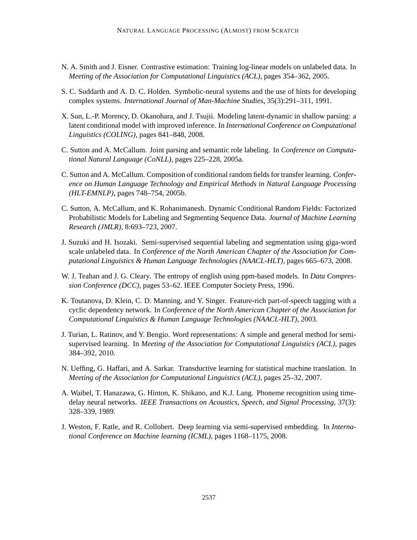
NATURAL LANGUAGE PROCESSING(ALMOST) FROM SCRATCH
N. A. Smith and J. Eisner. Contrastive estimation: Training log-linear models on unlabeled data. InMeeting of the Association for Computational Linguistics (ACL), pages 354–362, 2005.
S. C. Suddarth and A. D. C. Holden. Symbolic-neural systems and the useof hints for developingcomplex systems.International Journal of Man-Machine Studies, 35(3):291–311, 1991.
X. Sun, L.-P. Morency, D. Okanohara, and J. Tsujii. Modeling latent-dynamic in shallow parsing: alatent conditional model with improved inference. InInternational Conference on ComputationalLinguistics (COLING), pages 841–848, 2008.
C. Sutton and A. McCallum. Joint parsing and semantic role labeling. InConference on Computa-tional Natural Language (CoNLL), pages 225–228, 2005a.
C. Sutton and A. McCallum. Composition of conditional random fields for transfer learning.Confer-ence on Human Language Technology and Empirical Methods in NaturalLanguage Processing(HLT-EMNLP), pages 748–754, 2005b.
C. Sutton, A. McCallum, and K. Rohanimanesh. Dynamic Conditional Random Fields: FactorizedProbabilistic Models for Labeling and Segmenting Sequence Data.Journal of Machine LearningResearch (JMLR), 8:693–723, 2007.
J. Suzuki and H. Isozaki. Semi-supervised sequential labeling and segmentation using giga-wordscale unlabeled data. InConference of the North American Chapter of the Association for Com-putational Linguistics & Human Language Technologies (NAACL-HLT), pages 665–673, 2008.
W. J. Teahan and J. G. Cleary. The entropy of english using ppm-basedmodels. InData Compres-sion Conference (DCC), pages 53–62. IEEE Computer Society Press, 1996.
K. Toutanova, D. Klein, C. D. Manning, and Y. Singer. Feature-rich part-of-speech tagging with acyclic dependency network. InConference of the North American Chapter of the Association forComputational Linguistics & Human Language Technologies (NAACL-HLT), 2003.
J. Turian, L. Ratinov, and Y. Bengio. Word representations: A simple andgeneral method for semi-supervised learning. InMeeting of the Association for Computational Linguistics (ACL), pages384–392, 2010.
N. Ueffing, G. Haffari, and A. Sarkar. Transductive learning for statistical machine translation. InMeeting of the Association for Computational Linguistics (ACL), pages 25–32, 2007.
A. Waibel, T. Hanazawa, G. Hinton, K. Shikano, and K.J. Lang. Phonemerecognition using time-delay neural networks.IEEE Transactions on Acoustics, Speech, and Signal Processing, 37(3):328–339, 1989.
J. Weston, F. Ratle, and R. Collobert. Deep learning via semi-supervised embedding. InInterna-tional Conference on Machine learning (ICML), pages 1168–1175, 2008.
2537