NASA CONTRACTOR REPORT 187624 INDENTATION … · f / / =i • / nasa contractor report 187624 d indentation-flexure and low-velocity impact damage in graphite/epoxy laminates young

/ :

f / / =i• /

NASA CONTRACTOR REPORT 187624d

INDENTATION-FLEXURE AND LOW-

VELOCITY IMPACT DAMAGE IN

GRAPHITE/EPOXY LAMINATES

Young S. Kwon and Bhavani V. Sankar

UNIVERSITY OF FLORIDA

Gainesville, Florida

Grant NAG1-826

March 1992

National Aeronautics and

Space Administration

LANGLEY RESEARCH CENTERHampton, Virginia 23665-5225

(NASA-CR-ldTbZ_) INOENTATION-FLEXURE AND

L_W-VCL_CI[Y IMPACT OAMAG_ TN GnAPH!TE/_P_XY

LAMI_ATFS (Floridd Univ.) 171 p CSCL lID

_, 3124

N92-22967

https://ntrs.nasa.gov/search.jsp?R=19920013724 2018-12-01T03:07:33+00:00Z

TABLE OF CONTENTS

LIST OF TABLES .........................................

LIST OF FIGURES ........................................

CHAPTERS

1 INTRODUCTION .....................................

2 SPECMEN PREPARATION ..............................

Fabrication ......................................

Material Properties ..............................

3 STATIC INDENTATION TESTS .........................

Overview .........................................

Results and Discussion ...........................

Some General Observations on the

Load-Deflection Diagrams .....................

Loading up to Initial Observable

Failure ......................................

Ultrasonic C-Scan Results ......................

Loading, Unloading, and Reloading

Curves .......................................

Fractographic Studies ..........................stiffness Loss Due to Indentation

Damage .......................................

Analytical Models ................................

Delamination Pattern in Static Tests ...........

Strain Energy Release Rate .....................

4 LOW-VELOCITY IMPACT TESTS ........................

Background .....................................

Pendulum Impact Test Equipment ...............

Calibration of the Load Cell .................

Force-Displacement Relation ..................Results and Discussion .........................

Prediction of Impact Response

and Damage ...................................

5 SUMMARY AND DISCUSSION ...........................

page

iii

v

1

3

3

6

8

8

9

i0

17

22

26

26

29

31

31

33

35

35

35

37

40

42

43

52

i

Summary and Discussion ........................... 52

Conclusions ...................................... 55

APPENDICES

A SPECIMEN SUPPORT FIXTURE ......................... 57

B LOAD-DISPLACEMENT DIAGRAMS FOR

STATIC INDENTATION TESTS ....................... 59

C DATA FOR LOAD-DISPLACEMENT DIAGRAMS .............. 127

D DELAMINATION AREA ................................ 133

Static Indentation Test .......................... 133

Low-Velocity Impact Test ......................... 136

E FORCE HISTORY OF LOW-VELOCITY

IMPACT TESTS ................................... 137

REFERENCES ............................................. 159

ii

Table

2.1

4.1

B.I

B.2

B.3

C.I

D.I

D.2

D.3

D.4

D.5

D.6

E.I

E.2

E.3

LIST OF TABLES

page

39

Elastic constants from tensile tests .........

Dynamic calibration of load cell .............

Combination of indenter and support for

the static test on laminate type A ......... 59


the static test on laminate type B ......... 60


the static test on laminate type C ......... 61

Data for load-displacement diagrams of

static indentation tests ................... 128

Delamination area vs. static load

for laminate type A ........................ 133


for laminate type B ........................ 134


for laminate type C ........................ 135

Delamination area vs. impact load

for laminate type A ........................ 136


for laminate type B ........................ 136


for laminate type C ........................ 136

Results of impact test for laminate

type A ..................................... 137


type B ..................................... 137


type C ..................................... 138

iii

Figure

2.1

2.2

2.3

3.2

3.3

3.4

3.5

3.6

3.7

3.8

3.9

3.10

LIST OF FIGURES

Re-usable vacuum bag .........................

Vacuum bag layup for curing ..................

Curing cycle for Hercules carbonprepreg tape AS4/3501-6 ....................

Geometry of tensile test specimen ............

Typical load-deflection curve forgraphite/epoxy laminates ...................

Initial part of multiplereloading test .............................

The second part of multiplereloading test .............................

The third part of multiplereloading test .............................

The fourth part of multiplereloading test .............................

Static indentation test for laminatetype A:indenter-25.4mm dia.; support-50.8mm dia .................................

Static indentation test for laminatetype B:indenter-25.4mm dia.; support-50.8mm dia .................................

Static indentation test for laminatetype C:indenter-25.4mm dia.; support-

50.8mm dia .................................

Static indentation test for laminate

type A, B and C:indenter-25.4mm dia.;

support-50.8mm dia .........................

Sketch of load-displacement(P-q)

relation ...................................

v

page

4

4

5

7

i0

12

13

13

14

14

15

15

16

16

PRECEDING PAGE BLANK NOT FILMED .j

3.11

3.12

3.13

3.14

3.15

3.16

3.17

3.18

3.19

3.20

3.21

3.22

3.23

3.24

3.25

3.26

Failure load(P1) for laminate types

A, B and C .................................

Mohr's circle with the effect of

flexure ....................................

Center deflection(ql) at failure .............

Load drop(AP) at failure ....................

Secant modulus(K1) before failure ............

Delamination radius vs. maximum static

load for laminate type A ...................


load for lamiante type B ...................


load for laminate type C ...................

Samples of ultrasonic C-scan results:

(a)STAII (b)STA24 (c)STBI8 (d)STB20

(e)STC20 (f)STC22 ..........................

Schematics of delaminations and matrix

cracks:(a)laminate A; (b)laminate B;

(c)laminate C; and (d)laminate C.

Cases(a-c):after initial load drop;

Case(d):before load drop ...................

Typical view of matrix crack

initiation from a void during

loading(400x) ..............................

Matrix cracks and delamination formed

immediately after failure(100x) ............

Flexural test on damaged specimen

(STBI0) ....................................

Load-displacement curves from the

three-point bending tests for the

portions of damaged plate

(STBI0) ....................................

Contour of constant tensile principal

stresses for a unit load ...................

Slope of yield curve(K_) .....................

19

19

20

21

22

23

24

24

25

27

28

28

3O

3O

32

34

vi

4.1

4.2

4.3

4.4

4.5

4.6

4.7

4.8

4.9

4.10

4.11

4.12

4.13

4.14

A.I

Pendulum impact facility: (a)photo of

full setup and (b)schematic diagram

of setup ...................................

Definition of coordinate system ..............

Finite difference scheme .....................

Dynamic responses of laminate type A:

force-displacement curve ...................

Dynamic responses of laminate type B:


Dynamic responses of laminate type C:


Responses of laminate type A:

static and dynamic .........................

Responses of laminate type B:


Responses of laminate type C:


Delamination radius vs. maximum load

for laminate type A: static and dynamiccases ......................................

Delamination radius vs. maximum load

for laminate type B: static and dynamic

cases ......................................

Delamination radiuse vs. maximum load

for laminate type C: static and dynamiccases ......................................

Free body diagram of circular plate

under a concentrated impact load ...........

Impact force history for laminate

type C: impactor mass-13.98 Kg;

impact velocity-l.27 m/s ...................

Specimen support fixture:(a)photo of

fixture and (b)schematic diagram of

fixture ....................................

Load-displacement diagram of STAll ...........

Load-displacement diagram of STAI2 ...........

vii

36

38

41

46

46

47

47

48

48

49

49

5O

5O

51

58

63

64

B.3

B.4

B.5

B.6

B.7

B.8

B.9

B.10

B.II

B.12

B.13

B.14

B.15

B.16

B.17

B.18

B.19

B.20

B.21

B.22

B.23

B.24

B.25

B.26

B.27

B.28

Load-displacement dlagram of STAI3 ...........






Load-displacement,diagram of STAI9 ...........

Load-displacement diagram of STA20...........








Load-displacement dlagram of STA28...........





Load-displacement diagram of STB5............





Load-displacement dlagram of STBI0 ...........

viii

65

66

67

68

69

70

71

72

73

74

75

76

77

78

79

8O

81

82

83

84

85

86

87

88

89

90

B.29

B.30

B.31

B.32

B.33

B.34

B.35

B.36

B.37

B.38

B.39

B.40

B.41

B.42

B.43

B.44

B.45

B.46

B.47

B.48

B.49

B.50

B.51

B.52

B.53

B.54

Load-displacement diagram of STBII ...........

Load-displacement diagram of STBI2 ...........








Load-displacement diagram of STB20...........






Load-displacement diagram of STC5............





Load-displacement diagram of STCI0 ...........

Load-displacement diagram of STCII ...........




Load-displacement dlagram of STCI5 ...........

91

92

93

94

95

96

97

98

99

I00

I01

102

103

104

105

106

107

108

109

ii0

iii

112

113

114

115

116

ix

B.55

B.56

B.57

B.58

B.59

B.60

B.61

B.62

B.63

B.64

C.I

E.I

E.2

E.3

E.4

E.5

E.6

E.7

E.8





Load-displacement diagram of STC20...........






Sketch of typical load-displacementdiagram ....................................

Impact force history of IMPA5:(a)force vs. time and (b)force vs.displacement ...............................

Impact force history of IMPA7:(a)force vs. time and (b) force vs.displacement ...............................

Impact force history of IMPA9:(a)force vs. time and (b) force vs.displacement ...............................

Impact force history of IMPAI0:(a)force vs. time and (b)force vs.displacement ...............................

Impact force history of IMPAII:(a) force vs. time and (b)force vs.displacement ...............................

Impact force history of IMPAI2:(a)force vs. tlme and (b) force vs.displacement ...............................

Impact force history of IMPBI:(a)force vs. time and (b)force vs.displacement ...............................

Impact force history of IMPB2:

x

117

118

119

120

121

122

123

124

125

126

127

139

140

141

142

143

144

145

E.9

E.10

E.II

E.12

E.13

E.14

E.15

E.16

E.17

E.18

E.19

E.20

(a) force vs. time and (b)force vs.displacement ...............................

Impact force history of IMPB3:(a)force vs. time and (b)force vs.displacement ...............................

Impact force history of IMPBS:(a)force vs. time and (b) force vs.displacement ...............................


Impact force history of IMPB8:(a)force vs. time and (b) force vs.displacement ...............................


Impact force history of IMPCI:(a)force vs. tlme and (b)force vs.displacement ...............................

Impact force history of IMPC2:(a)force vs. time and (b)force vs.displacement ...............................

Impact force history of IMPC3:(a)force vs. time and (b) force vs.displacement ...............................

Impact force history of IMPC4:(a)force vs. time and (b)force vs.displacement ...............................


Impact force history of IMPC6:(a) force vs. time and (b) force vs.displacement ...............................


146

147

148

149

150

151

152

153

154

155

156

157

158

xi

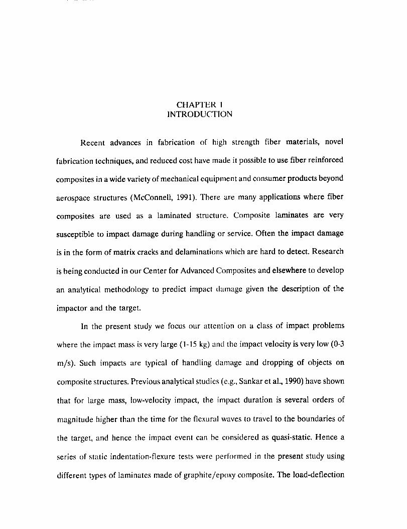
CHAPTER 1

INTRODUCTION

Recent advances in fabrication of high strength fiber materials, novel

fabrication techniques, and reduced cost have made it possible to use fiber reinforced

composites in a wide variety of mechanical equipment and consumer products beyond

aerospace structures (McConnell, 1991). There are many applications where fiber

composites are used as a laminated structure. Composite laminates are very

susceptible to impact damage during handling or service. Often the impact damage

is in the form of matrix cracks and delaminations which are hard to detect. Research

is being conducted in our Center for Advanced Composites and elsewhere to develop

an analytical methodology to predict impact damage given the description of the

impactor and the target.

In the present study we focus our attention on a class of impact problems

where the impact mass is very large (1-15 kg) and the impact velocity is very low (0-3

m/s). Such impacts are typical of handling damage and dropping of objects on

composite structures. Previous analytical studies (e.g., Sankar et al., 1990) have shown

that for large mass, low-velocity impact, the impact duration is several orders of

magnitude higher than the time for the flexural waves to travel to the boundaries of

the target, and hence the impact event can be considered as quasi-static. Hence a

series of static indentation-flexure tests were performed in the present study using

different types of laminates made of graphite/epoxy composite. The load-deflection

relationswere recorded.The damage was assessed by ultrasonic C-scanning and also

using photo-micrography. The static flexural response and damage were explained by

a simple semi-empirical model. Impact tests were performed, and the damage was

quantified using similar techniques. The relation between static and dynamic

responses was examined.

The descriptions of the material and fabrication procedures are given in

Chapter 2. The static test procedure and discussion of results form Chapter 3. Impact

tests and results are described in Chapter 4. A comprehensive summary and

conclusions are provided in Chapter 5. Complete experimental data and some

derivations of formulas used in the semi-empirical models are given in a series of

appendices.

2

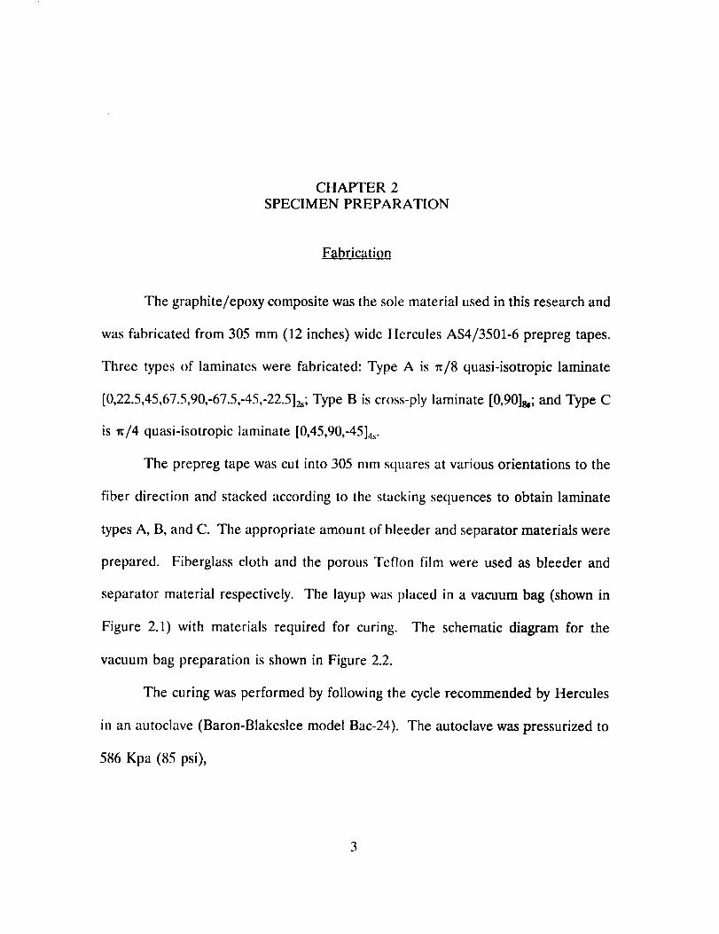
CHAPTER 2SPECIMEN PREPARATION

Fabrication

The graphite/epoxy composite was the sole material used in this research and

was fabricated from 305 mm (12 inches) wide ltercules AS4/3501-6 prepreg tapes.

Three types of laminates were fabricated: Type A is _x/8 quasi-isotropic laminate

[0,22.5,45,67.5,90,-67.5,-45,-22.5]z_; Type B is cross-ply laminate [0,90]_; and Type C

is re/4 quasi-isotropic laminate [0,45,90,-4514._.

The prepreg tape was cut into 305 mm squares at various orientations to the

fiber direction and stacked according to the stacking sequences to obtain laminate

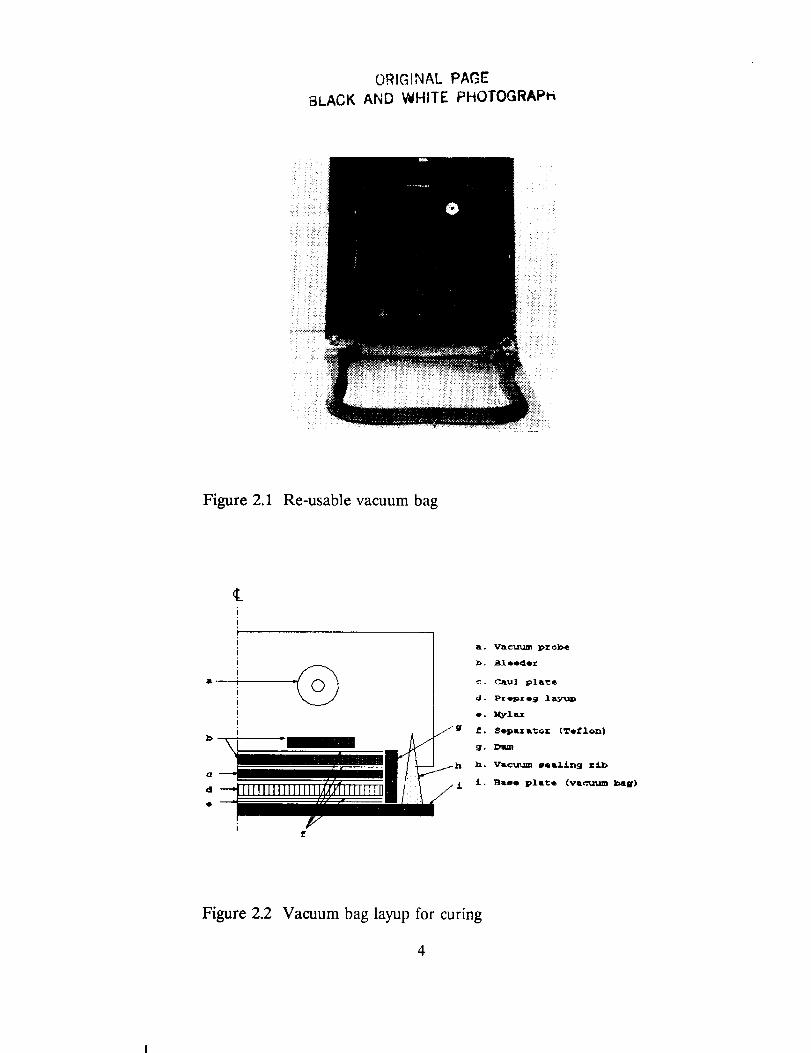
types A, B, and C. Tile appropriate amount of bleeder and separator materials were

prepared. Fiberglass cloth and the porous Teflon film were used as bleeder and

separator material respectively. The layup was placed in a vacuum bag (shown in

Figure 2.1) with materials required for curing. The schematic diagram for the

vacuum bag preparation is shown in Figure 2.2.

The curing was performed by following the cycle recommended by Hercules

in an autoclave (Baron-Blakeslee model Bac-24). The autoclave was pressurized to

586 Kpa (85 psi),

ORIGINAL PAGE

BLACK AND WHITE PHOTOGRAPh

Figure 2.1 Re-usable vacuum bag

b

d

@a. Vac%_d_ pzob•

. B1 oed•*"

o. My1 _.x

£. Sol_.z_Qz Creflon)

.qr,

Ix. VLeu_m e•Llln_ zlb

i. _aee pla_• (va_._En _g)

Figure 2.2 Vacuum bag layup for curing

4

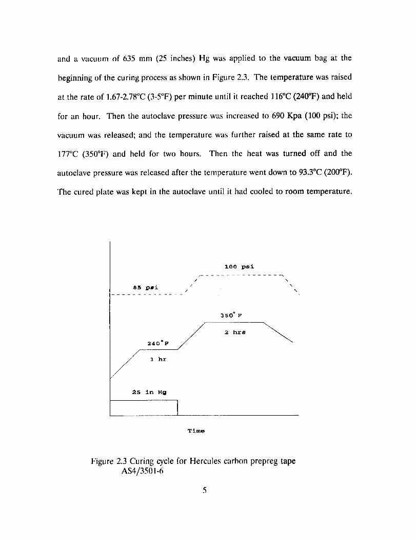
and a vacuum of 635 mm (25 inches) Hg was applied to the vacuum bag at the

beginning of the curing process as shown in Figure 2.3. The temperature was raised

at the rate of 1.67-2.78°C (3-5°F) per minute until it reached 116°C (240°F) and held

for an hour. Then the autoclave pressure was increased to 690 Kpa (100 psi); the

vacuum was released; and the temperature was further raised at the same rate to

177°C (350°F) and held for two hours. Then the heat was turned off and the

autoclave pressure was released after the temperature went down to 93.3°C (200°F).

The cured phtte was kept in the autoclave t, ntil it had cooled to room temperature.

I00 psi

/ \

/ \85 Dei /

o240 F

I hz

350 ° F

2 hrs

25 in Hg

Time

Figt, re 2.3 Curing cycle for Hercules carbon prepreg tape

AS4/3501-6

Material Properties

The properties of the composite material were provided by the prepreg

mantffacturer. Tensile tests were performed to verify the quality of fabrication.

The specimen preparation and tensile tests were performed according to

AS'I'M standard D3039-76 (ASTM, 1987). The specimen is straight-sided, of constant

cross-section, and has adhesively bonded, beveled tabs for gripping. The lamina 0 °

test specimen is 12.7 mm (0.5 inches) in width and six plies in thickness, while the

lamina 90 ° test specimen is 25.4 mm (1 inches) in width and eight plies in thickness.

The overall length of the specimen is 228.7 mm (9 inches), and the test section is

152.4 mm (6 inches). The test specimen geometry is shown in Figure 2.4.

The wedge-section friction grips were utilized for the tensile loading on MTS

material tester. The specimen was loaded monotonically to failure at a rate of 2

mm/min. Electrical resistance strain gages were mounted on the specimen to

determine the specimen strains in fiber and transverse directions. The strain gages

were monitored by digital oscilloscope, Nicolet 4094. Stress-strain curves were

plotted to obtain the Young's moduli and Poisson's ratios.

Five tensile tests were conducted for 0 ° and 90 ° test specimens. The results

are presented in Table 2.1.

The 0 ° tensile modulus at room temperature provided by the manufacturer is

148 Gpa. Thus the quality of the composite fabricated for this research is proven to

be fairly adequate.

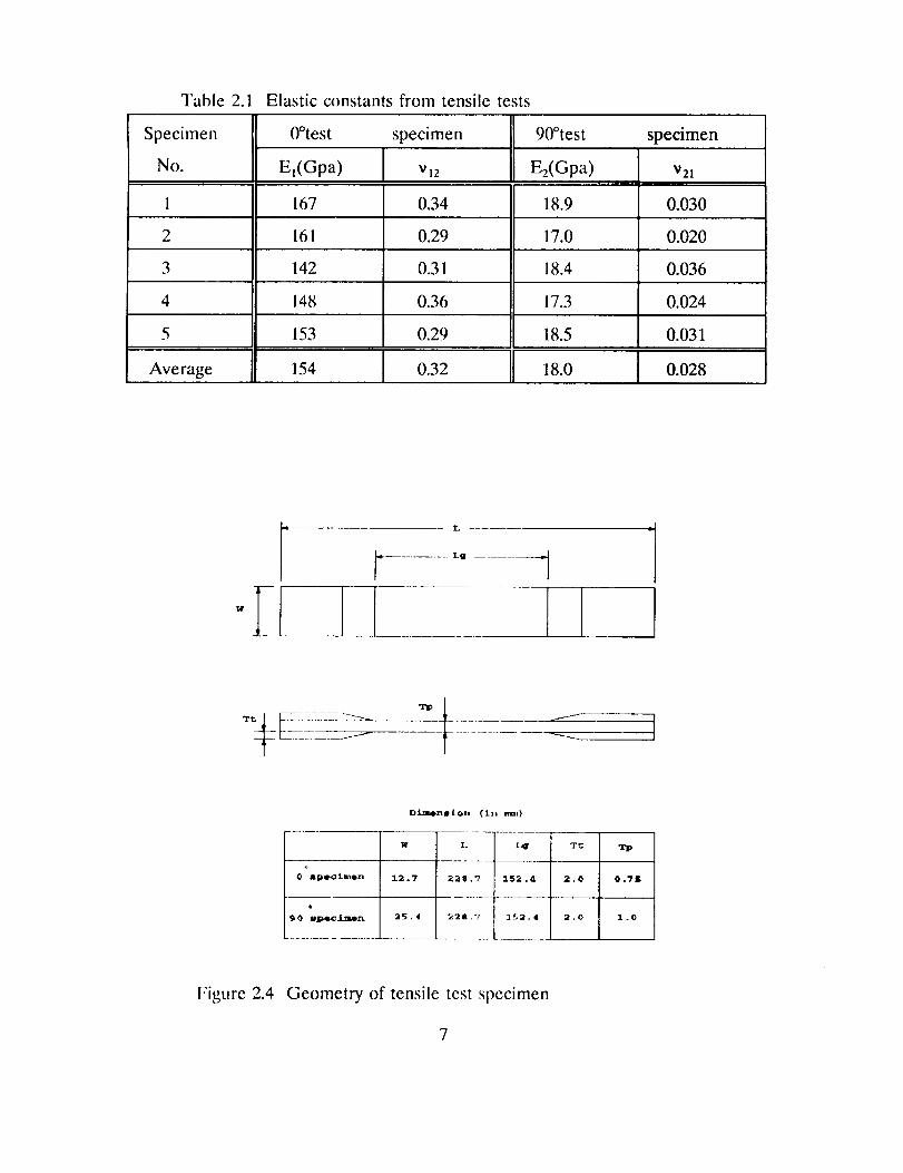
Table 2.1 Elastic constantsfrom tensile tests

Specimen

No.Jl

1

0°test specimen 90°test

El(Gpa) v]z Ez(Gpa)

167 0.34 18.9

2 161 0.29 17.0

3 142 0.31 18.4

4 148 0.36 17.3

Average

153 0.29 18.5

154 0.32 ]]18.0

specimen

V21

0.030

0.020

0.036

0.024

0.031

0.028

+

0 IIDOO:I.II_On

9 O epec.t.mezx

Dimo=mto. (in ram}

W L I 14J T_ T_

3.2.7 22S .'7 I 152.4. 2,0 O.?S

25.4 228.7 I 152.4 2.0 1.0

Figure 2.4 Geometry of tensile test specimen

7

CHAPTER 3STATIC INDENTATION TESTS

Overview

This chapter describes static indentation tests performed on graphite/epoxy

laminates in order to gain a better understanding of damage initiation and

progression in plates of different sizes and laminate configurations due to indentation

by different diameter indenters. It is expected that a thorough understanding of the

damage due to static indentation will shed light on damage mechanisms during

impacts due to large masses at low velocities.

As mentioned in Chapter 2, three types of laminate configurations were used:

Type A is _r/8 quasi-isotropic laminate [0,22.5,45,67.5,90,-67.5,-45,-22.5]zs; Type B is

cross-ply laminate [0,90]8,; and Type C is _r/4 quasi-isotropic laminate [0,45,90,-45]4 _.

Square specimens were cut from cured laminates. The sides of the specimens were

about an inch longer than the diameter of the support rings used in the indentation

tests. Thus the specimens can be considered as simply supported circular plates. The

support ring diameters were 50.8 mm, 76.2 mm, and 101.6 mm. The two steel

indenters had hemispherical nose of diameters 6.35 mm and 25.4 mm respectively.

The indentation test setup consisted of a loading apparatus, recording devices

and data processing devices as given below:

- MTS Material Tester

- Digital Oscilloscope(Nicolet 4094& XF-44 Recorder)

- LVDT (Schaevitzmodel 500 MHR)

- Analog Transducer Amplifier (Schaevitzmodel ATA-101)

- SpecimenSupport Fixture (seeAppendix A)

- Computing Facilities (VAX mainframe and microcomputers)

The testswere conductedunder stroke control at the rate of 0.02mm/s. The

load and plate center deflection datawere acquired at the rate of 5 samples/second

and were recorded by the Nicolet XF-44 recorder. The data were transferred to a

microcomputer from the oscilloscopeandwere processedbysoftwareavailable in the

mainframe and in the microcomputer.

After indentation tests the specimenswere C-scannedat a facility at NASA

Langley ResearchCenter. Someof the specimenswere sectionedand polished for

the purposeof photo-micrographicstudies.The damagewasalso assessedby cutting

small beam specimensout of the damagedarea and testing them under three-point

flexure.

Resvlts and Discussions

The load-deflection diagrams of all the tests are presented in Appendix B.

Some plots are presented in Figures 3.1 through 3.9 for the purpose of discussion.

The general observations about the indentation damage and effects of layup, plate

diameter, and indenter diameter are discussed in the following section.

9

Some General Observations on the Load-Deflection Diagrams

There are some common features in the load-deflection diagrams for the three

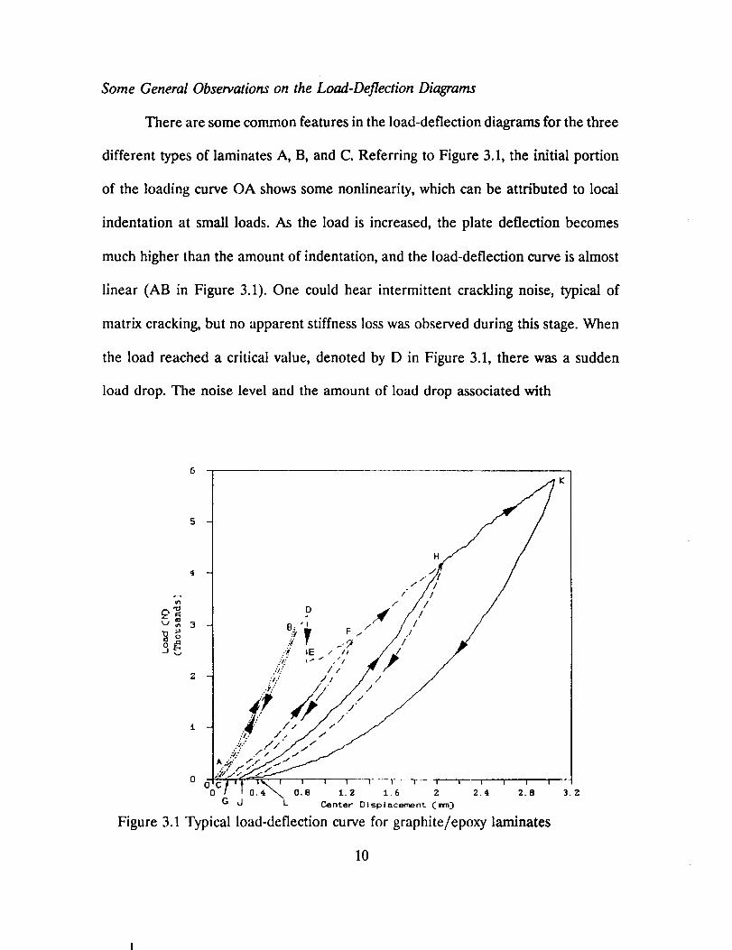
different types of laminates A, B, and C. Referring to Figure 3.1, the initial portion

of the loading curve OA shows some nonlinearity, which can be attributed to local

indentation at small loads. As the load is increased, the plate deflection becomes

much higher than the amount of indentation, and the load-deflection curve is almost

linear (AB in Figure 3.1). One could hear intermittent crackling noise, typical of

matrix cracking, but no apparent stiffness loss was observed during this stage. When

the load reached a critical value, denoted by D in Figure 3.1, there was a sudden

load drop. The noise level and the amount of load drop associated with

0 I I I I I I I I

0 0.6 1.2 1,6 2 2,4 2.8

G d L Center Displacement (era:)

Figure 3.1 Typical load-deflection curve for graphite/epoxy laminates

10

failure (see Figures 3.6-3.9 for comparison) were highest for the cross-ply laminates

(Type B), lowest in the _/8 quasi-isotropic laminates (Type A), and in-between in

the _/4 quasi-isotropic laminates (Type C). It is suspected that the load drop is

caused by initiation and unstable propagation of delaminations.

After the first observable failure, there is a significant loss of plate stiffness

denoted by the reduced slope of the subsequent unloading and reloading curves, e.g.,

FG and GF, HJ and JH, etc in Figure 3.1. As will be seen later, the delaminations

grow in a stable manner as the load is increased. The loading curve EFHK

represents yielding of the plate and hence will be called the yield curve. The yield

curve is almost a straight line until the central deflection is about 3 mm (note that

the average plate thickness is 3.8 ram). Thereafter there is a sudden increase in the

slope of the yield curve (e.g., Figures 3.6-3.9). The slopes of the unloading curves

at this stage are sometimes greater than the stiffness of the undamaged plate and

were highly nonlinear also. The nonlinearities can be attributed to (a) large

deflection of the plate; (b) membrane action in the delaminated plies; and (e)

friction between various contacting surfaces, e.g., between the indenter and the plate,

between delaminations, and between the plate and the support.

Some specimens were unloaded evet_ heft)re the first observable failure (BC

in Figure 3.1), and there were some energy losses indicated by the hysteresis loop

(area OBC). This energy loss can be attributed mainly to material damage, and to

some extent to friction at contact areas. When unloaded at higher loads, the

unloading anct reloading curves were highly nonlinear (e.g., FG and GF, HJ and JH).

11

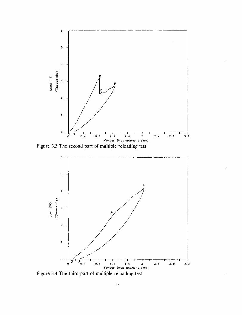
The area between the corresponding unloading and reloading curves, e.g., FG and

GF, is the measure of frictional energy dissipation. The area between an unloading

curve and the next reloading curve, e.g., FG and JH, is an example of energy

dissipation due to material damage, mostly delaminations.

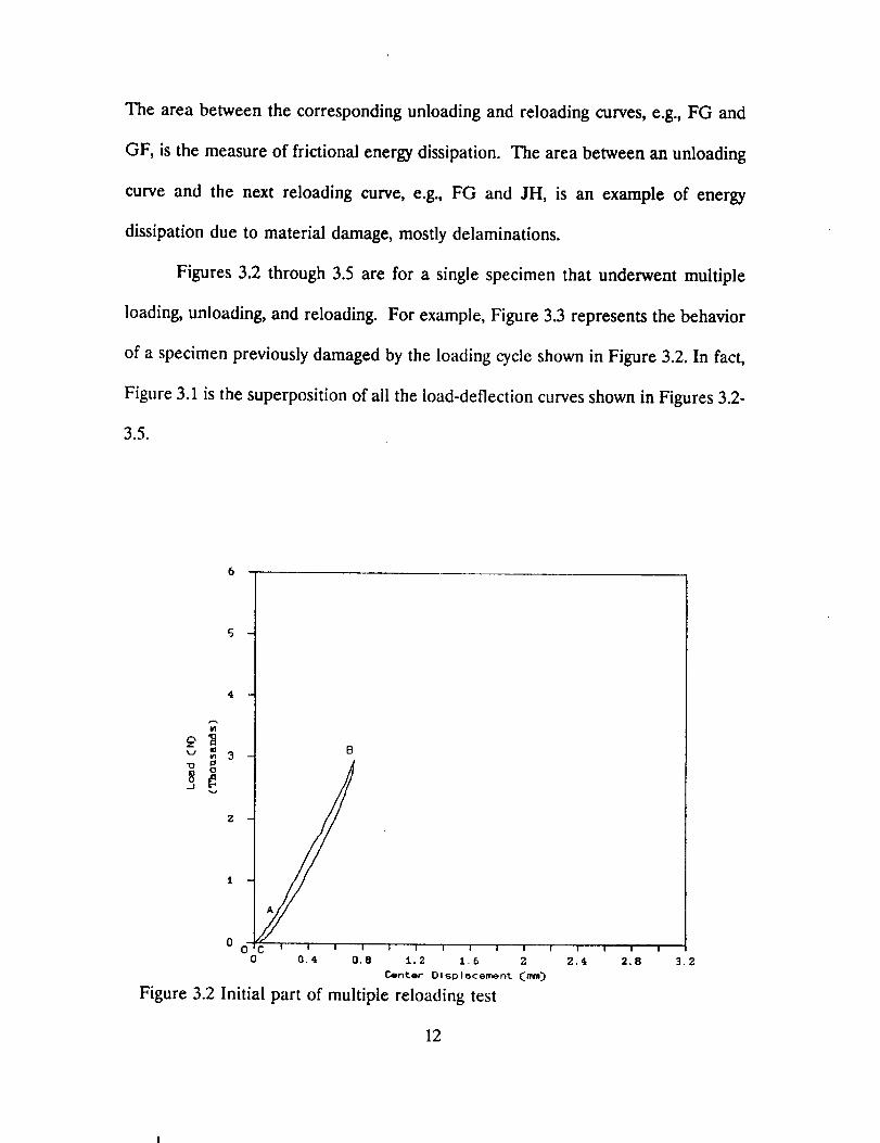
Figures 3.2 through 3.5 are for a single specimen that underwent multiple

loading, unloading, and reloading. For example, Figure 3.3 represents the behavior

of a specimen previously damaged by the loading cycle shown in Figure 3.2. In fact,

Figure 3.1 is the superposition of all the load-deflection curves shown in Figures 3.2-

3.5.

u _ 3

S__.1

B

C i i i I

o 0.4 o,8I I I I I I

1.2 1.6 2

Oenter Olsplacemen% (_rnm_)

Figure 3.2 Initial part of multiple reloading test

12

I I I I

2.4 3,8 3.

_3°v

| I I I I ! I I I I I

0 0.4 0.8 1.2 1.6 2 2.4

Center Olsplncement Cram)

Figure 3.3 The second part of multiple reloading test

I !

2.8 3.2

H

4

o

2

l

0 G ij = I = 1 I = _ = =0 0.4 0.8 1.2 1,6 2

Center Dlsplecement Cmm_)

Figure 3.4 The third part of multiple reloading test

I I I I I

2.4 2. B 3.2

13

v

0

0 0.4 0.8 1.2 1.6 2

Center Dlsplscement Clnm:)

Figure 3.5 The fourth part of multiple reloading test14

13

12

1t

10

9

_ _ 7•u m

J_" 5

4

3

2

1

0

2.4 2.8 3,2

STAll

STA13

STA14 ......................

STA15 .....

! I

2

Center Displacement Cmm)

Figure 3.6 Static indentation test for laminate type A:indenter-25.4 mm dia.;

support-50.8 mm dia.

14

12

11

10

9

@

_5

4

3

2

t

Q

STB5

S'TB6 .......................

5"TB7 ......

5TB8

0 6

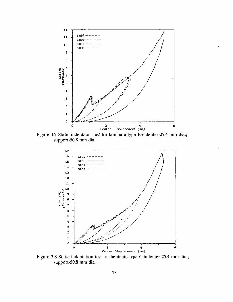
Figure 3.7 Static indentaion test for laminate type B:indenter-25.4 mm dia.;


t7

16

15

14

13

12

11

_10ta

D _ 8

dE-, 7

6

S

t

3

2

1

0

STC5

STC6 ..................

SIC? .......

STC8

I I ! I

0 2 4 6

Center Ol6placement Cmm)

Figure 3.8 Static indentation test for laminate type C:indenter-25.4 mm dia.;


15

17

t65"TA .....................

iS5"IB

t4 STC --

13

12

Ii

,.-,10

_ 8O

?

6

5

4

3

Z

1

0

I

,,/)/f

//

I

I

//

I I I I

0 Z _ 6

Canter Displacement (mm)

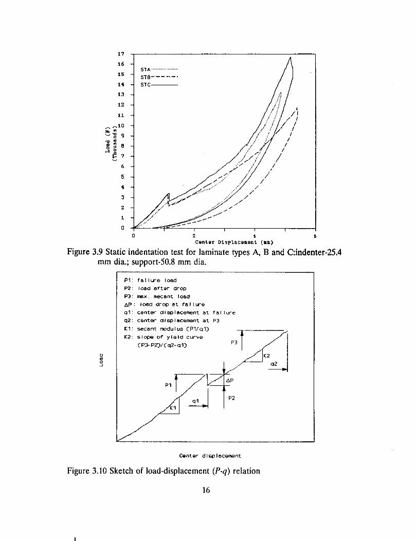
Figure 3.9 Static indentation test for laminatc types A, B and C:indentcr-25.4

mm dia.; support-50.8 mm dia.

o

o_i

PI: fnllure Iond

P2: IoaO _fter drop

P3: max. secant Iond

_p: load drop 8t failure

ql: center dlspl_cemen*_ a_ fal lure

q2: cen_er CIIsplacement at P3

KI: secant rrK)dulu5 (Pl/cll)

K2: slo_ of yleld curvo _

(P3- P2rJ/(q2-q 1) P3/ /1// I

Center d I Gp I acement

Figure 3.10 Sketch of load-displacement (P-q) relation

16

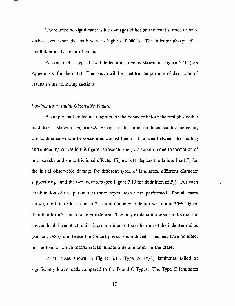
There were no significant visible damageseither on the front surfaceor back

surfaceeven when the loadswere as high as 10,000N. The indenter alwaysleft a

small dent at the point of contact.

A sketch of a typical load-deflection curve is shown in Figure 3.10 (see

Appendix C for the data). The sketch will be used for the purpose of discussion of

results in the following sections.

Loading up to hz#ial Observable Failure

A sample load-deflection diagram for the behavior before the first observable

load drop is shown in Figure 3.2. Except for the initial nonlinear contact behavior,

the loading curve can be considered almost linear. The area between the loading

and unloading curves in this figure represents energy dissipation due to formation of

microcracks and some frictional effects. Figure 3.11 depicts the failure load P1 for

the initial observable damage for different types of laminates, different diameter

support rings, and the two indenters (see Figure 3.10 for definition of P1). For each

combination of test parameters three repeat tests were performed. For all cases

shown, the failure load due to 25.4 mm diameter indenter was about 30% higher

than that for 6.35 mm diameter indenter. The only explanation seems to be that for

a given load the contact radius is proportional to the cube root of the indenter radius

(Sankar, 1985), and hence the contact pressure is reduced. This may have an effect

on the load at which matrix cracks initiate a delamination in the plate.

In all cases shown in Figure 3.11, Type A 0r/8) laminates failed at

significantly lower loads compared to the B and C Types. The Type C laminates

17

(7r/4) performed better than the cross-ply laminates (Type B) under the 50.8 rnm ring

support, but failed at slightly lower loads under 76.2 and 101.6 mm supports.

It seems that the interlaminar shear stresses in conjunction with the flexural

stresses are responsible for initiation of delaminations. The interlaminar shear stress

distribution (r=) is parabolic away from the contact region but skewed very near the

contact region (Sankar, 1989). If there were only shear stresses, the matrix material

will be subjected to tensile stresses (principal stresses) in the 45 ° planes, which are

responsible for the matrix cracks (see Mohr's circle in Figure 3.12). The effect of

flexure is to add a compressive normal stress (a=) above the mid-plane and tensile

normal stress below the mid-plane of the laminate. The compressive stresses will

reduce the magnitude of the principal stresses and hence delay the onset of

transverse cracks. The larger the support ring diameter, the larger are the flexural

stresses. This could explain the increase in failure loads for Type A and Type B

laminates with increase in the support ring diameter. The failure loads for 7r/4

laminates were slightly reduced with the increase in the support ring diameter. This

suggests that there is a need for a detailed stress analysis of laminates under

indentation-flexure in order to understand the initiation of mierocracks and

delaminations.

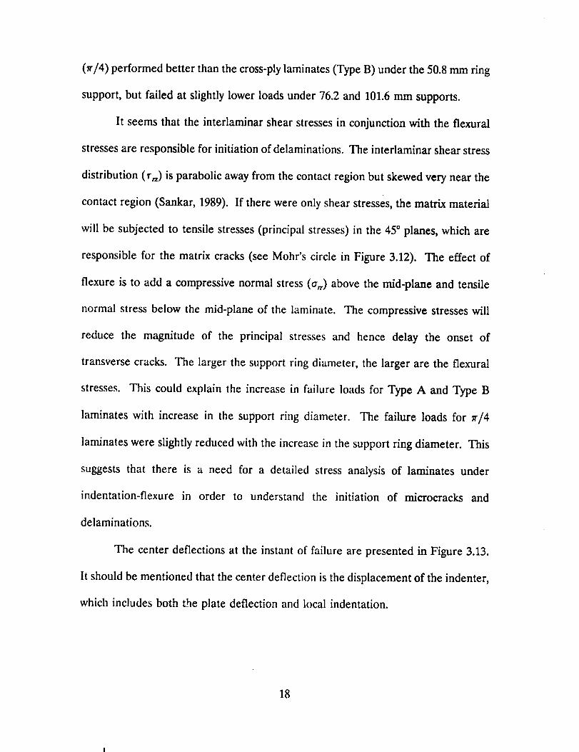
The center deflections at the instant of failure are presented in Figure 3.13.

It should be mentioned that the center deflection is the displacement of the indenter,

which includes both the plate deflection and local indentation.

18

4,5

3.5

o_,_J

1.5

0,5

Indenter:l 6.35 tr_ dla. + 25,4 mm dla.

A B C +I I

* *---4 * _ " +.-............... . _+_-- --. ..... ,..4, +I _#_ ................. I

"[ • ....I......................................._:_ + I I

I I + •

l .........L. _ _ ...... i.-.... -_=__ ......_ ..............•.... + •

_ __._ ! + • _ ................liil..........•i • i "

i •

A B Ci i

A B C

050.8 mm 75.2 mm

Sup_oort O Io_neter

Figure 3.11 Failure load(Pz) for laminate types A, B and C

101,6 mm

Figure 3.12 Mohr's circle with the effect of flexure

19

2,6

Indenter:l 6,35 mm dla, 4- 25.4 mm dla,

2.4

2,2

2

_ "1, 8u

cl.6o

iJul,4@

1,2

l

0.8

0.6

0.4

O.Z

0

A B c

÷ ;"-. I+ ,

+

• +

¢+

I i

_ _ L__.J

A B C

I

Ii

ii |+I

I

i ++ •

i •I

i • +

I

i L___J L__-J

A BI

I

iI

iI

iI

I

I

I

I

+

I

c

50.8 mm ?6.2 rnm

SUpport OI ameCer

Figure 3.13 Center deflection (qt) at failure

101.6 mm

1.5

t.4

1.3

1.g

1.1

1

..-, O, 9

_ _o,7_0.6

0.5

0.4

0.3

0.2

0.1

0

Indenter:l 6.35 mm dla, + 25.4 mm dla.

A B C A B C A B C

+ + I I

...... .i 2"'_-,_ -+- - i ++ ...... i .......... + .... i_ _ - _

• ,-..

I ..... ,..,. +i + ..... -t.. +

i + i ................

+ I II i ....................t I +

• I • ij ............. i..... I +

+

50,8 mm 76.2 n_n

Support Diameter

Figure 3.14 Load drop (alP) at failure

• i • t •i ...... _ ......

mr.......... 1................ • ........... _ ....... •

+ , i ...............• I i ............

i II !, i, ii i

I

I

i +

!l q

I ,101,6 mm

20

It is interesting to see that for a given support ring size, the center deflection

at failure does not depend on the indenter diameter very much.

After the unstable failure, there is a significant load drop in the displacement

controlled tests. The load drop for different sets of test parameters are shown in

Figure 3.14. In general the load drop is higher, if the failure load is higher. The rr/8

laminates do not show much load drop, which indicates that the failure is not sudden,

but similar to yielding of ductile materials. The load drop in the case of cross-ply

laminates is in general higher than for the 7r/4 quasi-isotropic laminates.

The flexural stiffness of the undamaged laminates (kl) under different test

conditions is shown in Figure 3.15. It is interesting to note that the stiffness is

apparently greater under the 25.4 mm indenter than the 6.35 mm indenter. The

bigger indenter causes larger contact area and lesser indentation. Since indentation

is also included in the deflection, the apparent stiffness of the plate is higher for

larger diameter indenter. In fact the effect of indenter size diminishes for larger plate

diameters. Type C laminates have the highest flexural stiffness, and Type A have the

lowest.

As the loading continues, the delaminations caused by the initial failure

continue to grow in a stable manner. Before we discuss the unloading and reloading

tests, it will be instructive to look at the ultrasonic C-scan results.

21

Indenter:l 6.35 mm dla. + 25,4 mm dla.

4.S

3.5

3z.5ffl

o 2

r,¢

1.5

0.S

+

+

+

+

| •+

I

A B C

A B C

+

J/ *

I I

A B

"_; I

50.8 mm 76,2 mm

Suppor _ Ol mmeter

Figure 3.15 Secant modulus (/{'1) before failure

101.6 mm

C

+

¢

I

Ultrasonic C-Scan Results

The damaged specimens were C-scanned to map the area of delamination.

The damage pattern was almost circular in all cases. This may be due to the quasi-

isotropic nature of the laminates and the circular support used in the tests. In Figure

3.18 the delamination radii are plotted against the maximum contact force applied

during the test for _r/4 laminates (Type C). In the case of Type C laminates the

delamination radius was directly proportional to the maximum load irrespective of

the indenter size or the plate size. A linear relation between the delamination radius

and the maximum load was obtained using least square curve fitting. There were

some scatter in the data for the Type A and Type B laminates as seen in Figures 3.16

22

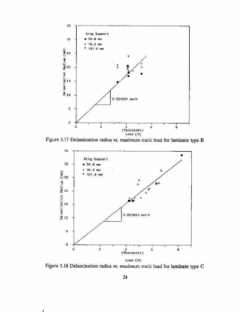
and 3.17. However it was decided to use a linear fit for all the results. The

delamination radius b can be expressed as b=BP,,,=, where B is the .constant of

proportionality. The constant B in mm/N units for the _r/8, cross-ply and 7r/4

laminates respectively were found as 0.005295, 0.004334, and 0.003863. Thus one can

see that 7r/4 laminates have better delamination resistance than cross-ply laminates,

and cross-ply laminates are better than 7r/8 laminates.

The data for delamination areas are presented in Appendix D. Sample C-scan

outputs are shown in Figure 3.19.

35

3O

z5k.J

tO

_ 20

C0

t.J

C

Ring Support

a 50.8 mm

+ 76.2 mm

o 101.6 mm+

° i/+

+ 0

0.005295 mnVN

() -- I f T ...... T i 1 i

0 2 4 6 8

(Thousands)

Load (I_)

Figure 3.16 Delamination radius vs. maximum static load for laminate type A

23

35

30

z5kJ

_zot-O

,o

c

E

RI nu SUDPort

• 50.8 mm

+ 76.2 mm

o 101.6 mm

+o

0.004334 n_N

I I i I I I I

0 2 4 6 8

(Thousands)

toad < NJ

Figure 3.17 Delamination radius vs. maximum static load for laminate type B

3O

r"N

L,,25

IBD

2oc

0

_a

C

N to

+

°

0,003863 n_n/N

I I I I I I I I

0 2 4 6 8

(Thousands)

Load CN)

Figure 3.18 Delamination radius vs. maximum static load for laminate type C

24

ORIGINAL PAGE

BLACK AND WHITE PHOTOGRAPH

(a)

"fl'l'ifi Ni .... ., ...i,.;.2 i::

......._ " .... :?._:: :_:._ .... :_:: _._:_!.,.'.!_._' ._ i-'i:'_ _':..-..E_,._

(c)

g'tr ........ ri'/'l'nlr ............................. - ..........

(e)

_.. -._ _-_ v:._:;_:_:.:s_:::_

•.x.. "_" :: "_:i_:!:::-'__!_:!_i!"._:i_.'.'_i_i:i:i:i:i:i_::: :: :i:i_'_i: :_

_'.. _ ,:" •.,::_.:_ -:v:.• ,.:,: .... :.- .:., .:,. :+:+:.:.:,_,

(b)

(d)

]: _:::.':..:._:" . .._ .. . . ..:

(0

Figure 3.19 Samples of ultrasonic C-scan results: (a)STA11 (b)STA24 (c)STB18

(d)STB20 (e)STC20 (f)STC22

25

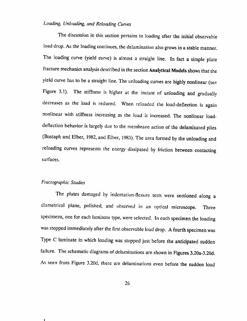
Loading, Unloading, and Reloading Curves

The discussion in this section pertains to loading after the initial observable

load drop. As the loading continues, the delamination also grows in a stable manner.

The loading curve (yield curve) is almost a straight line. In fact a simple plate

fracture mechanics analysis described in the section Analytical Models shows that the

yield curve has to be a straight line. The unloading curves are highly nonlinear (see

Figure 3.1). The stiffness is higher at the instant of unloading and gradually

decreases as the load is reduced. When reloaded the load-deflection is again

nonlinear with stiffness increasing as the load is increased. The nonlinear load-

deflection behavior is largely due to the membrane action of the delaminated plies

(Bostaph and Elber, 1982, and Elber, 1983). The area formed by the unloading and

reloading curves represents the energy dissipated by friction between contacting

surfaces.

Fractographic Studies

The plates damaged by indentation-flexure tests were sectioned along a

diametrical plane, polished, and observed in an

specimens, one for each laminate type, were selected.

optical microscope. Three

In each specimen the loading

was stopped immediately after the first observable load drop. A fourth specimen was

Type C laminate in which loading was stopped just before the anticipated sudden

failure. The schematic diagrams of delaminations are shown in Figures 3.20a-3.20d.

As seen from Figure 3.20d, there are delaminations even before the sudden load

26

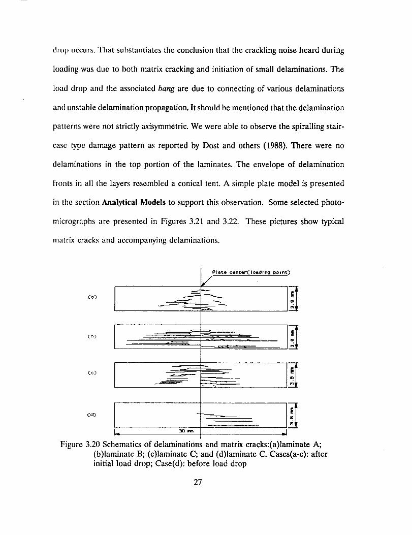
drop occurs. That substantiates the conclusion that the crackling noise heard during

loading was due to both matrix cracking and initiation of small delaminations. The

load drop and the associated bang are due to connecting of various delaminations

and unstable delamination propagation. It should be mentioned that the delamination

patterns were not strictly axisymmetric. We were able to observe the spiralling stair-

case type damage pattern as reported by Dost and others (1988). There were no

delaminations in the top portion of the laminates. The envelope of delamination

fronts in all the layers resembled a conical tent. A simple plate model is presented

in the section Analytical Models to support this observation. Some selected photo-

micrographs are presented in Figures 3.2l and 3.22. These pictures show typical

matrix cracks and accompanying delaminations.

Plete center(_ Ioedl ng 1oolrrt_)

/

Figure 3.20 Schematics of delaminations and matrix cracks:(a)laminate A;

(b)laminate B; (c)laminate C; and (d)laminate C. Cases(a-c): after

initial load drop; Case(d): before load drop

27

ORIG!N,_L PAGE

i3LACK AND WHllE PHOTOGR_H

Figure 3.21 Typical view of matrix crack initiation from a void during

loading(400x)

Figure 3.22 Matrix cracks and delamination formed immediately afterfailure(100x)

28

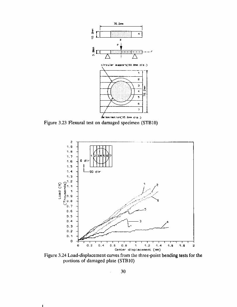
Stiffness Loss Due to Indentation Damage

One of the plates subjected to indentation was sectioned into several beams,

and the flexural rigidities of the damaged beams were measured using three-point

bending tests. The specimen considered was a cross-ply laminate (Specimen Number

STB10). The support ring diameter was 50.8 mm, and the indenter diameter was

25.4 mm. The loading-unloading diagram for this laminate is given in Appendix B.

The damaged plate was sectioned into seven beams. The width of each beam was

about 10.2 mm, and the span for the three-point bending tests was 50.8 mm as shown

in Figure 3.23. The load-deflection diagrams obtained from the three-point bend

tests are shown in Figure 3.24. Beam 1 is undamaged and represents the stiffness of

the intact plate. Beams 2 and 6 are symmetrical about the center and have the same

amount of damage. Beam 4, which was at the center of the laminate, had suffered

severe damage in the indentation test as indicated by the reduced stiffness in flexure.

The residual stiffness information from such tests will be useful in verifying damage

models that may be developed in the future.

29

76.2ram

r 1_ [I Ii!::i::!!iii::!iii_:.!!_i!i::!::_l4T"

Z

/X i A

circular eUl04oor_50.Smm clla.)

2

r-

!i

..._]

die I_ f nmt r on( 35.6m,._ dD-,.)

Figure 3.23 Flexural test on damaged specimen (STB10)

2

1.9

1.8

1.?

1.6

1.5

1.4

1.3

r,1.2

0 _0.9_J_---o.8

0,7

0.6

0.5

0.4

0.3

0.2

0.1

0

1 2

.,11..-' ..,.-:"."-'" f

....;.;" .--" 5

<.:" ,"i, ,./

_;'::;" ,.'"'" -- 3

• j,,

, , , , , , , , ; , , , , , , , , ,

O 0,2 0.4 0.6 0,8 1 1.2 1.4 1.6 1.8 2

Center d 15p I acement _mm)

Figure 3.24 Load-displacement curves from the three-point bending tests for the

portions of damaged plate (STB10)

30

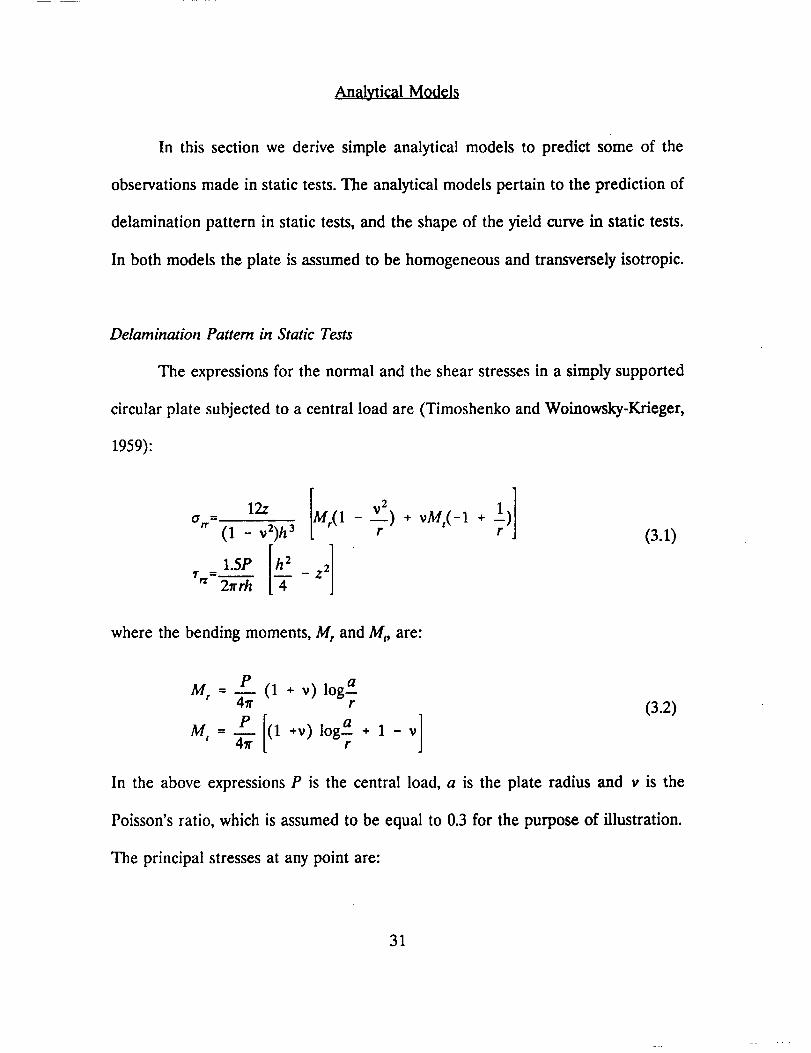
Analytical Models

In this section we derive simple analytical models to predict some of the

observations made in static tests. The analytical models pertain to the prediction of

delamination pattern in static tests, and the shape of the yield curve in static tests.

In both models the plate is assumed to be homogeneous and transversely isotropic.

Delamination Pattern in Static Tests

The expressions for the normal and the shear stresses in a simply supported

circular plate subjected to a central load are (Timoshenko and Woinowsky-Krieger,

1959):

12z IMp(1a,_-- (1 - v2)h 3 (3.1)

where the bending moments, M, and Mr, are:

Mr = t9 (1 + v)log a4rt r

M' = P--4_r[(1 +v)loga +lr -v]

(3.2)

In the above expressions P is the central load, a is the plate radius and v is the

Poisson's ratio, which is assumed to be equal to 0.3 for the purpose of illustration.

The principal stresses at any point are:

31

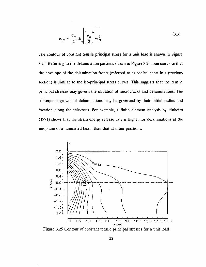
O'rr 2

O"1,2 2 + frz

(3.3)

The contour of constant tensile principal stress for a unit load is shown in Figure

3.25. Referring to the delamination patterns shown in Figure 3.20, one can note that

the envelope of the delamination fronts (referred to as conical tents in a previous

section) is similar to the iso-principal stress curves. This suggests that the tensile

principal stresses may govern the initiation of microcracks and delaminations. The

subsequent growth of delaminations may be governed by their initial radius and

location along the thickness. For example, a finite element analysis by Pinheiro

(1991) shows that the strain energy release rate is higher for delaminations at the

midplane of a laminated beam than that at other positions.

1,6 "

1.2 _.

0.8

0.4

_' 0.0 ....

-0.4

-0.8

-1.2

-1.6

-2.0

I I I I I I I I I i I i I l I I I I I I I

0.0 1.5 3.0 4.5 6.0 7.5 9.0 10.5 12.0 13.5 15.0r Cm3

Figure 3.25 Contour of constant tensile principal stresses for a unit load

32

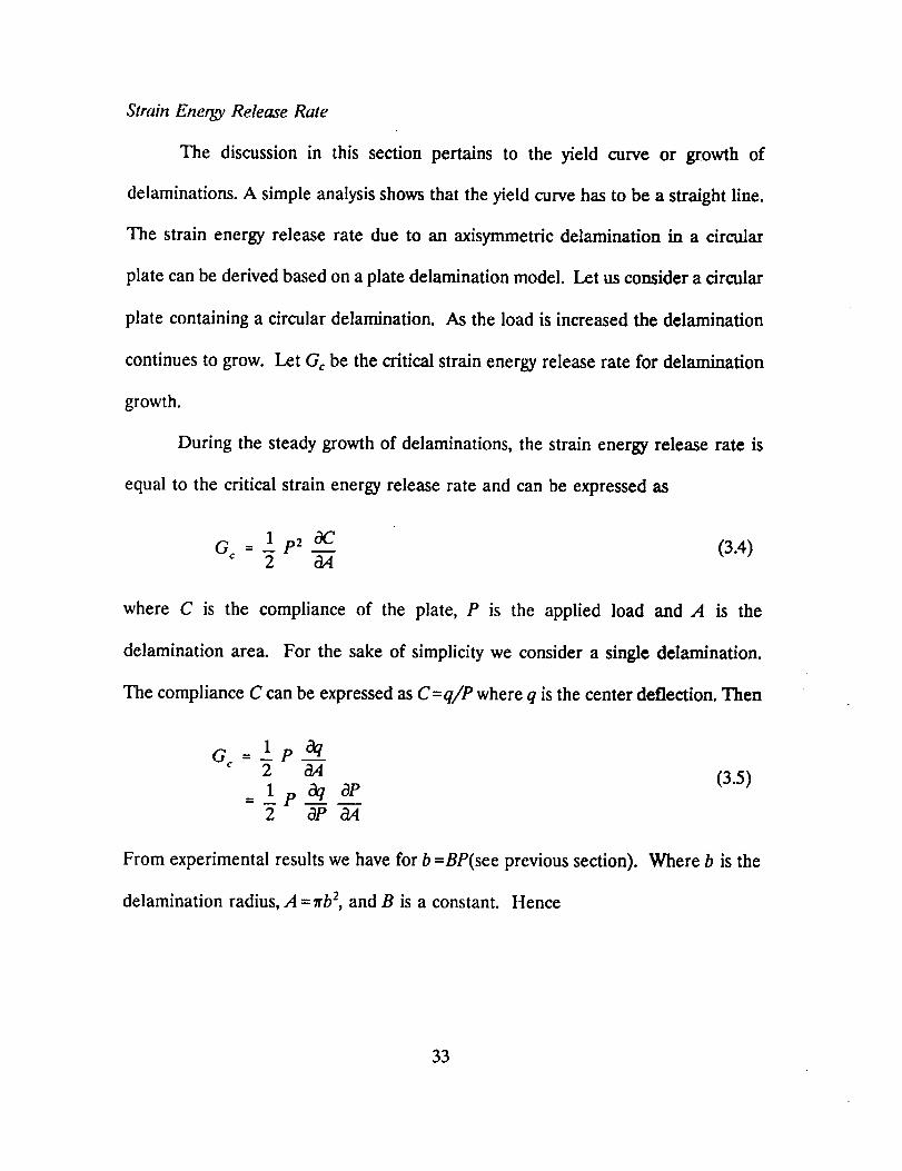
Strain Energy Release Rate

The discussion in this section pertains to the yield curve or growth of

delaminations. A simple analysis shows that the yield curve has to be a straight line.

The strain energy release rate due to an axisymmetric delamination in a circular

plate can be derived based on a plate delamination model. Let us consider a circular

plate containing a circular delamination. As the load is increased the delamination

continues to grow. Let Gc be the critical strain energy release rate for delamination

growth.

During the steady growth of delaminations, the strain energy release rate is

equal to the critical strain energy release rate and can be expressed as

Gc = 1p2 8C (3.4)2 8,4

where C is the compliance of the plate, P is the applied load and A is the

delamination area. For the sake of simplicity we consider a single delamination.

The compliance C can be expressed as C =q/P where q is the center deflection. Then

G : _1e__+2 8,4 (3.5)1 8q dP_- _e2 OP &4

From experimental results we have for b =BP(see previous section). Where b is the

delamination radius, A = 7rb2, and B is a constant. Hence

33

d,,t 2_rB2p (3.6)0P

Substituting in (5) we obtain

If G¢ is assumed to be a constant for the particular material and lay-up, then we find

that ,3P/Ct/ must also be a constant. The term &t,/_ is actually the slope of the

yield curve, e.g., FHK in Figure 3.1. Test results from various plates have shown that

the yield curve is indeed a straight line. The values of the slope, K2, for various

combinations of test parameters are shown in Figure 3.26.

2.6

Indonter:• 6.35 mm dla, 4. 25,4 mm dla.

2.4

2.2

2

1.8

1.6/-%

N

0.8

0.6

0.4

0.2

0

+

+

+ •

- I •

+• +

-- +

• +

- •

A 8 C

50.8 mm

Figure 3.26 Slope of yield curve (/(2)

i

I

I

I

I+

I

I

' II

I

I •

I +

iis

il+i +t

I

I

i A 8iiI

I

i

I

+ I

i+ I ÷

+ I +

I

I

t +I ij • •I + • •

I + •

I

i•i •I

!•I

C i A B CI

I

iI

76.2 mm

Support Diameter

101.6 mm

34

CHAP'IER 4

LOW-VELOCITY IMPACT TESTS

B_at maad

Low-velocity impact tests were conducted on composite laminates in order to

compare the response and damage with corresponding behavior under static loading.

The laminate types, indenter, and support ring diameters were the same as used in

static tests. The equipment used in impact studies consisted of the following:

- Pendulum Impact Facility

- Digital Oscilloscope (Nicolet 4094 & Nicolet XF-44 Recorder)

- Computing Facilities; VAX mainframe and microcomputers

Pendulum Impact Test Equipment

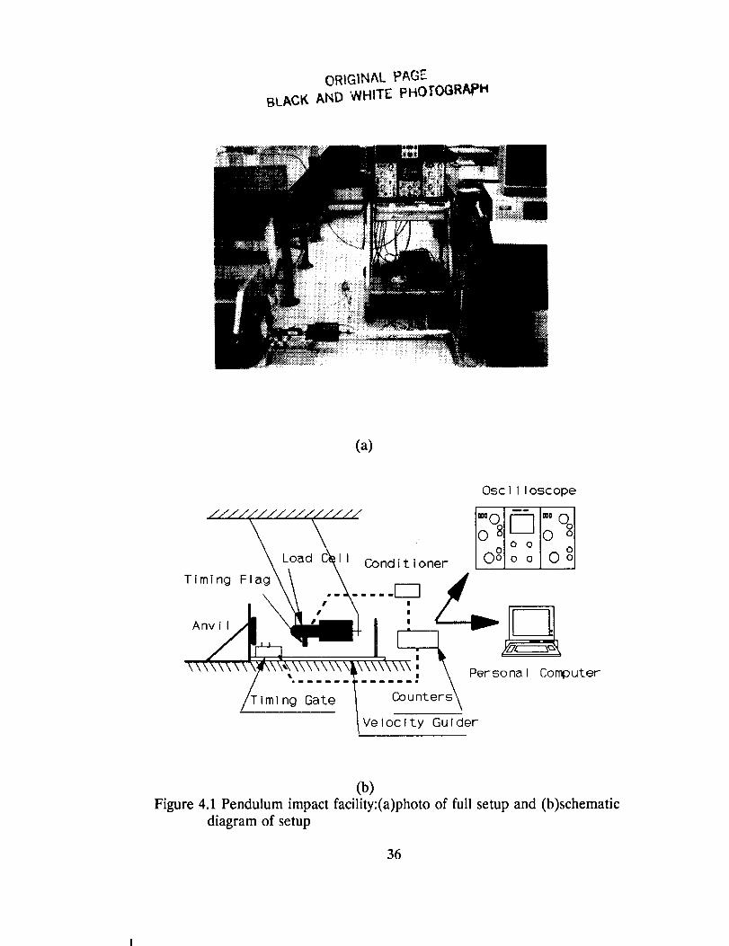
The impact pendulum is depicted in Figure 4.1. It is a modified version of the

one described by Sj6blom, Hartness, and Cordell (1988). It is easier to measure the

rebound velocity of the impactor in a pendulum impact facility than in a drop tower

impact facility. The impact and rebound velocities were measured by using two pairs

of phototransistors and light emitting diodes with two 10 MHz counters. The impact

force was measured by using an instrumented tup, Dynatup 8496-1, and a Vishay

2310 strain gage conditioner. The digital oscilloscope, Nicolet 4094, was used for

35

ORIGINAL PAGE

BLACK AND WHITE pHOTOGRAPH

(a)

Osci I oscope

//////////////// I,-,,,01 _ I®. O I

\ \ . o 81_1ooO\ \ I olO O l o I

\Load C_ll Conditioner O°I°° Io o

Timing Flag . ._111i{__/_

//T,m, no Gate _ _cou nt_ers__

(b)Figure 4.1 Pendulum impact faci]ity:(a)photo of full setup and (b)schematic

diagram of setup

36

recording the impact force history during the event. The personal computer was also

utilized to record the impact and rebound velocities and to compute the impact

energy and energy imparted to the target. A gauge was used to measure the drop

height of the impactor to ensure repeatable impacts. The maximum velocity

obtainable was about 2 m/s. The maximum mass the tup can carry was about 15 kg.

The support for the specimen was fixed on the anvil mechanically. The support used

for the pendulum impact facility was the same ring support used for the static

indentation tests described in the previous chapter. Only the 50.8 mm diameter ring

support was used in impact studies.

Calibration of the Load Cell

According to Ireland (1974), it is necessary to calibrate the load cell

dynamically for the instrumented impact testing. The different components in the

load cell might react differently due to the differences in load introduction rates

between static and impact loading. Having the impact and the rebound velocities

measured, we can calibrate the load cell dynamically so that the average force is

correct. Consider the impact event depicted in Figure 4.2. Assume that the load is

proportional to output signal.

F,, = C/7= (4.1)

I_ : _-F a dt = m(Vr-Vi)(4.2)

37

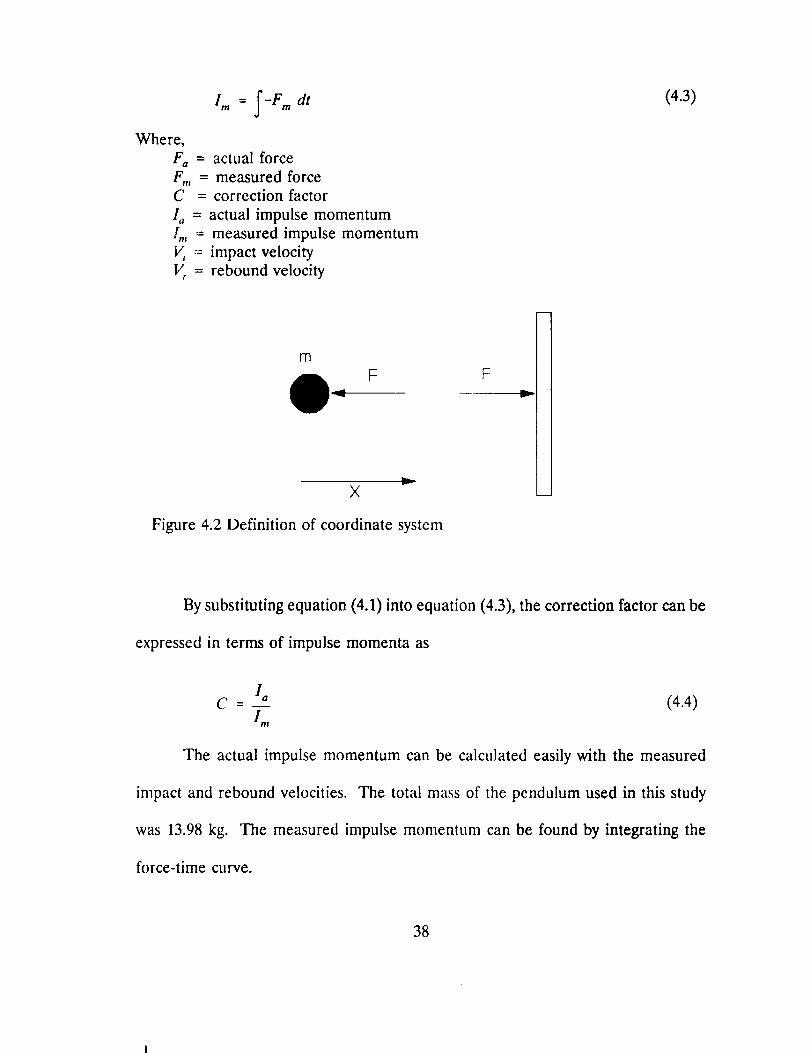
Im = _-F,,, dt

Where,

Fa = actual force

F,, = measured forceC = correction factor

16 = actual impulse momentum

I,, = measured impulse momentum

V_ = impact velocity

Vr = rebound velocity

(4.3)

m

F F

v

v

×

Figure 4.2 Definition of coordinate system

By substituting equation (4.1) into equation (4.3), the correction factor can be

expressed in terms of impulse momenta as

a

C = n (4.4)Im

The actual impulse momentum can be calculated easily with the measured

impact and rebound velocities. The total mass of the pendulum used in this study

was 13.98 kg. The measured impulse momentum can be found by integrating the

force-time curve.

38

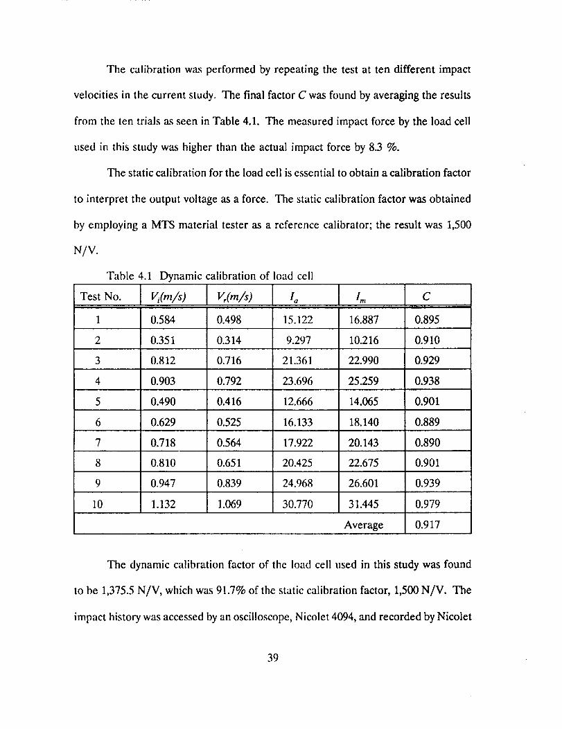
The calibration w,_s performed by repeating the test at ten different impact

velocities in the current study. The final factor C was found by averaging the results

from the ten trials as seen in Table 4.1. The measured impact force by the load cell

used in this study was higher than the actual impact force by 8.3 %.

The static calibration for the load cell is essential to obtain a calibration factor

to interpret the output voltage as a force. The static calibration factor was obtained

by employing a MTS material tester as a reference calibrator; the result was 1,500

N/V.

Table 4.1 Dynamic calibration of load cell

Test No. Vi(m/s ) V,(rn/s) Io I,,, Ci

0.5841 0.498 15.122 16.887 0.895

2 0.351 0.314 9.297 10.216 0.910

3 0.812 0.716 21.361 22.990 0.929

4 0.903 0.792 23.696 25.259 0.938

5 0.490 0.416 12.666 14.065 0.901

6 0.629 0.525 16.133 18.140 0.889

7 0.718 0.564 17.922 20.143 0.890

8 0.810 0.651 20.425 22.675 0.901

9 0.947 0.839 24.968 26.601 0.939

10 1.132 1.069 30.770 31.445 0.979

Average 0.917

The dynamic calibration factor of the load cell used in this study was found

to be 1,375.5 N/V, which was 91.7% of the static calibration factor, 1,500 N/V. The

impact history was accessed by an oscilloscope, Nicolet 4094, and recorded by Nicolet

39

XF-44 Recorder. The impact history was simply the force-time curve, and the force

was measured in voltage difference by the load cell and multiplied by dynamic

calibration factor to obtain the true impact force.

Force-Displacement Relation

From the experimentally measured impact force history, and the impact

velocity, a relation between the contact force and impactor displacement can be

derived. The governing equation for the impact problem is defined as:

rrff,= -F(t)x(O) = 0

-- V0

(4.5)

where m is the impactor mass, x is the impactor displacement, V o is the initial

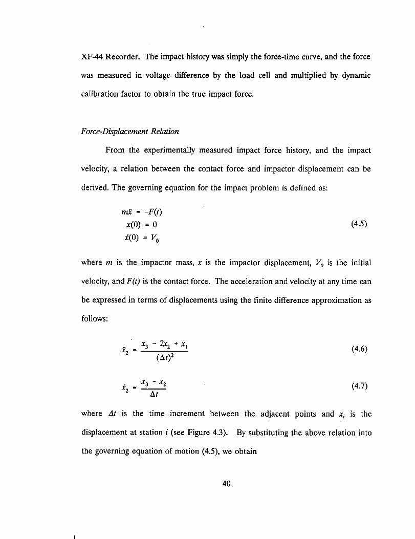
velocity, and F(t) is the contact force. The acceleration and velocity at any time can

be expressed in terms of displacements using the finite difference approximation as

follows:

x 3 - 2x 2 + x 1x2 " (4.6)

(At) 2

"_2 " X3 - X2 (4.7)At

where At is the time increment between the adjacent points and x_ is the

displacement at station i (see Figure 4.3). By substituting the above relation into

the governing equation of motion (4.5), we obtain

40

m(x 3 - 2x 2 + xI)= _Fz (4.8)

(At) 2

Solving for x3,

-F2(At) 2 (4.9)x 3 - + 2x 2 - x 1

m

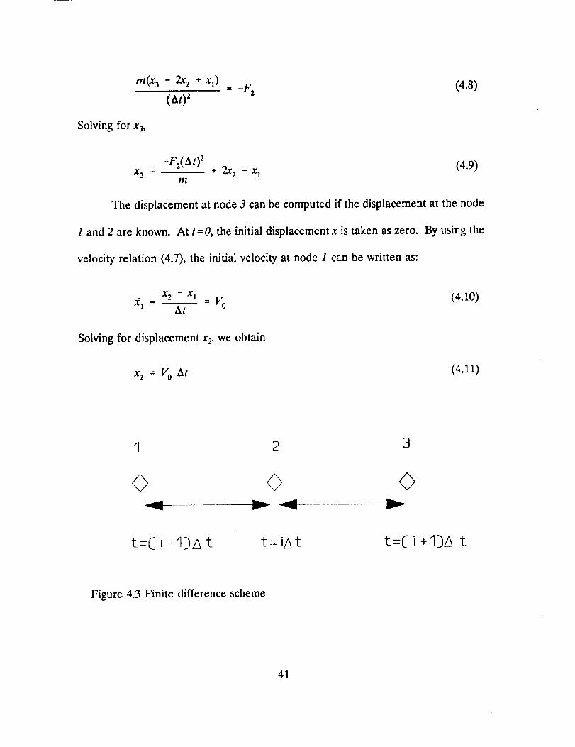
The displacement at node 3 can be computed if the displacement at the node

1 and 2 are known. At t=O, the initial displacement x is taken as zero. By using the

velocity relation (4.7), the initial velocity at node 1 can be written as:

x2 - xl (4.10)iI " At = V°

Solving for displacement x2, we obtain

x 2 = V0 At (4.11)

1 2 3

t=( -qbAt t= iAt t=( i+l)A t

Figure 4.3 Finite difference scheme

41

Results and Discussion

The impact force history (F-t) and corresponding force-deflection (F-q)

relations for all the tests conducted are presented in Appendix E. The results also

include the impact energy and the energy imparted to the specimen. The energy

imparted is actually equal to the difference between the initial and final kinetic

energies of the impactor computed from the impact and rebound velocities.

The contact force-deflection relations from some of the impact tests for the

three types of laminates are presented in Figures 4.4-4.6. The dynamic load-

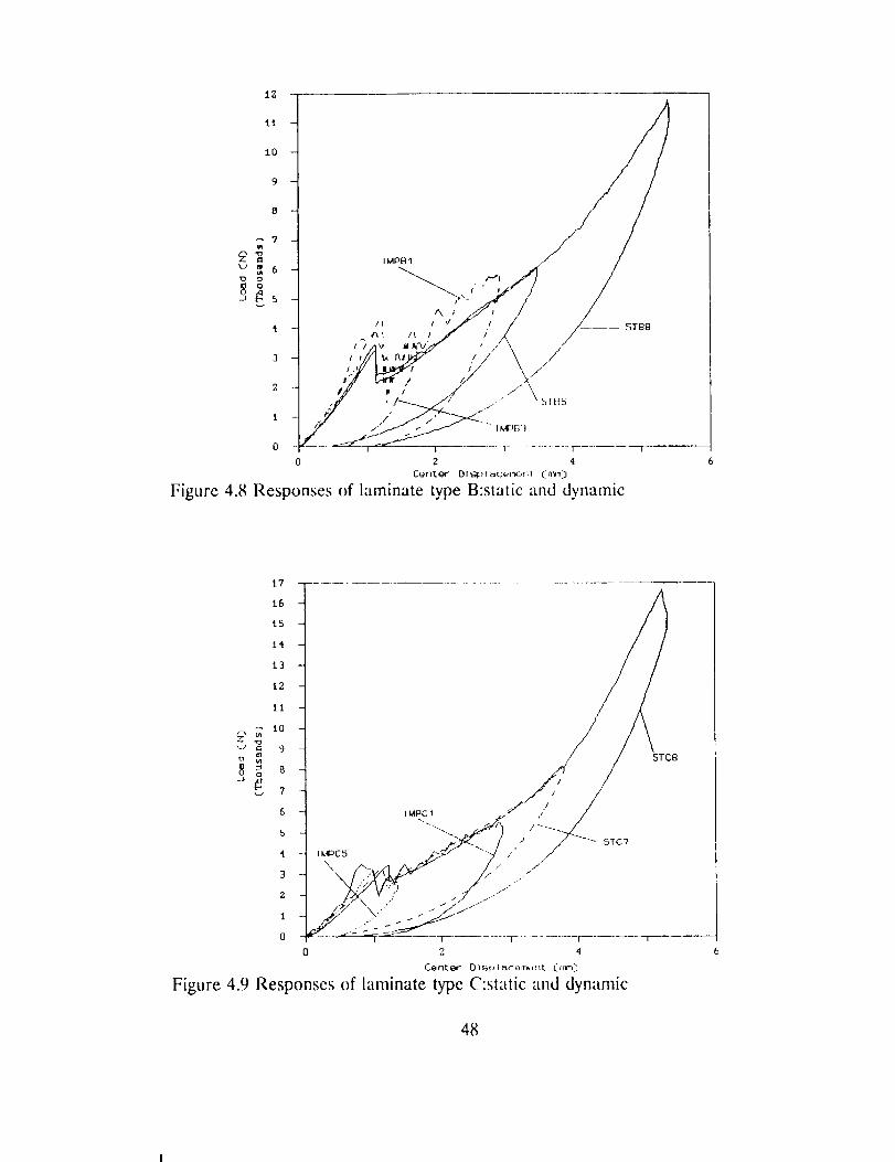
deflection behavior is compared with corresponding static behavior in Figures 4.7-4.9.

Until the initial failure indicated by the sudden load drop, the dynamic stiffness was

slightly higher than the static stiffness k 1. After the initial failure the load-deflection

relations followed the static curves. Types B and C' showed some high frequency

oscillations superposed over the static curves. Type A laminates displayed a yielding

point as they did in static tests. In Type A laminates, yielding occurred at the same

load as in the static tests for low impact velocities (%<0.77 m/s). However, for

higher velocities (Vo> O.77 m/_) yielding occurred at a lower load (see Figure 4.4 for

comparison), and the load-deflection relatio_s deviated from the static curves

considerably. It is not clear if this was due to variations in the specimens.

The _treas of delamination in impacted specimens were measured using

ultrasonic C-scanning. The results are prcscntcd in Appcmlix D along with results

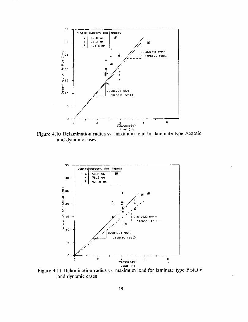
from static tests. In Figures 4.10-4.12 the dclamination radii are plotted against the

maximum contact force experienced by the specimen during impact. These figures

42

display corresponding static resultsalso. The delamination radii are found to be

proportional to the maximum force. A least square curve fitting of impact data

shows that in all three types of laminates, the delamination radius for a given

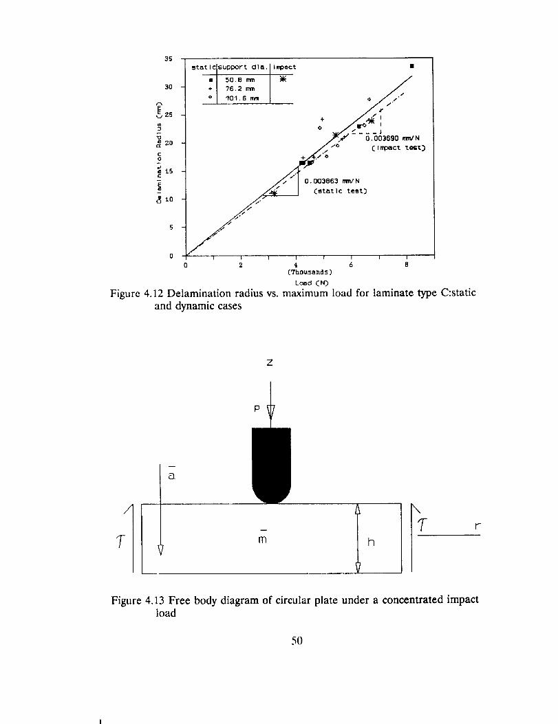
maximum contact force is slightly lower in impact tests than in static tests.The

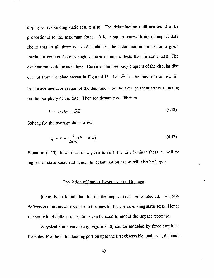
explanationcould be asfollows. Considerthe free body diagramof the circular disc

cut out from the plate shownin Figure 4.13. Let m be the mass of the disc,

be the average acceleration of the disc, and r be the average shear stress r,_ acting

on the periphery of the disc. Then for dynamic equilibrium

P - 27rrhr = ma (4.12)

Solving for the average shear stress,

1 - - (4.13)= r- (e - ma)" 27rrh

Equation (4.13) shows that for a given force P the interlaminar shear r,_ will be

higher for static case, and hence the delamination radius will also be larger.

Prediction of Impact Res.'ponse and Damage

It has been found that for all the impact tests we conducted, the load-

deflection relations were similar to the ones for the corresponding static tests. Hence

the static load-deflection relations can be used to model the impact response.

A typical static curve (e.g., Figure 3.10) can be modeled by three empirical

formulas. For the initial loading portion upto the first observable load drop, the load-

43

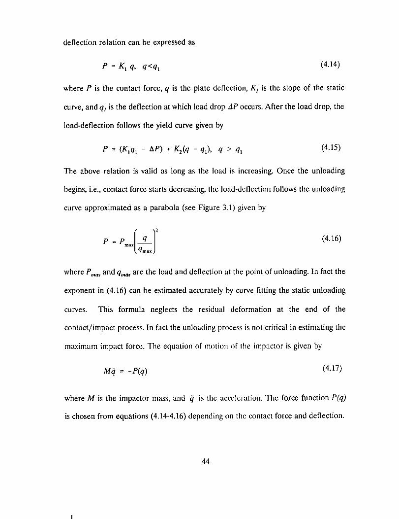
deflection relation can be expressedas

P = Kl q, q<ql (4.14)

where P is the contact force, q is the plate deflection, K 1 is the slope of the static

curve, and ql is the deflection at which load drop AP occurs. After the load drop, the

load-deflection follows the yield curve given by

P = (Klq 1 - AP) + K2( q -q,), q > ql (4.15)

The above relation is valid as long as the load is increasing. Once the unloading

begins, i.e., contact force starts decreasing, the load-deflection follows the unloading

curve approximated as a parabola (see Figure 3.1) given by

P = P.,.x ----q--q (4.16)all'laX

where P,,,_ and q,,_ are the load and deflection at the point of unloading. In fact the

exponent in (4.16) can be estimated accurately by curve fitting the static unloading

curves. This formula neglects the residual deformation at the end of the

contact/impact process. In fact the unloading process is not critical in estimating the

maximum impact force. The equation of motion of the impactor is given by

MO = -P(q) (4.17)

where M is the impactor mass, and /_ is the acceleration. The force function P(q)

is chosen from equations (4.14-4.16) depending on the contact force and deflection.

44

The equation of motion can be numerically integrated to obtain force-time

history. The constants K 1, qp ziP and K 2 are obtained from one simple static test.

The above procedure was tried for several impact tests and the agreement between

the measured and predicted impact response, in particular the maximum contact

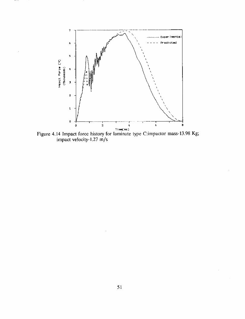
force, was excellent. A sample comparison is shown in Figure 4.14. Now from the

maximum predicted contact force, one can predict the delamination radius using the

C-scan results for the static tests. The delamination radius obtained using C-scan for

impact tests on Type C laminates is plotted in Figure 4.12 along with corresponding

static results. For a given maximum contact force, the delamination radius in impact

tests is slightly smaller than in static tests. Thus static tests provide a conservative

estimate of the delamination radius.

45

o_o

_ 3

m_

I_PA5

IMPA7 ......

I_PA9 .......................

IMPAIi .................

I ..,/"

//

/./

/

,// /

J

T [ I

0 i 2 3

Center Displacement (mm)

Figure 4.4 Dynamic responses of laminate type A:force-displacement curve

IIfPBI /_

: /v /(D 01 II"0u _

0 I I I '¢ I t - ----]----7- t i 1 1

0 O.'t 0. B 1.2 _.6 Z 2.q 2.8

Center Dlsplacement (mm)

Figure 4.5 Dynamic responses of laminate type B:force-displacement curve

46

,.-, 4

14'1

U I:i

O

tOla-,

Im

H 2

IIITC1

I_PC3 ...............

I_[PC5 ...................

I_PC6 .....

I I I I I

O 0.4 0.8 1.2 1.6 Z Z.4 2.8

Center Dlsplacement (mm)

Figure 4.6 Dynamic responses of laminate type C:force-displacement curve

14

u

10

O_1

13

_z

10

9

_ 7

5

4

2

1

0

IMPA11

IPA9

Figure 4.7 Responses of laminate type A:static and dynamic

47

lZ

it

lO

9

, x: ,,:'>/'// / _,o_3 I If/It, nly'// / / \ /

;.f_ _< \/_p" L-_r / //" ,_

0 l T l

2 'i

C_,n'r._"Dl_plac,em_-nc Crn_

Figure 4.8 Responses of laminate type B:static and dynamic

].7 .................

t6

i5

i4

1.3

1.2

tl

©_, to

_ STC8

8g a-J _ 7

6

5

4

3

2

1

0 .... T V I

o 2 4

C_intl_r" Dl_lJl_icorrltnt _rll'Tl_

Figure 4.9 Responses of laminate type C:static {tlld dynamic

48

35

t0 2 4 6 8

(Thousands)

Load (N)

Figure 4.10 Delamination radius vs. maximum load for laminate type A:staticand dynamic cases

25

30

/7

_s

2o

"/ so.o-- I'/ 76.2..,° I

/ / £___ I r impact test)

/ ,,." I o.oo4a34 _m,' N

---. I0 T.... ] r T..... ] ........ r----i ..... , ,

2 4 6 8

('r'o.ousa nd s )

Load (N)

Figure 4.11 Delamination radius vs. maximum load for laminate type B:staticand dynamic cases

49

35

statlcsupport Ella, Impect •

• 50,8 mm _K /

+1 76.2 mm I /J30 °l Iol.6_ I /

_/___J

20 _ io C Ir_:_c'L x.el_t:)

_ .4".- I °'°°_ _"- /.4_'" I Cstat Ic te_t?

0 I I I I I t I I

0 2 4 6 9(Thousands)

Load CN')

Figure 4.]2 De]amination radius vs. maximum load for laminate type C:static

and dynamic cases

:7

/

a

m Ih\

'7 r-

Figure 4.13 Free body diagram of circular plate under a concentrated impactload

5O

5

Figure 4.14 Impact force history for lamin_te type C:impactor mass-13.98 Kg;

impact ve!ocity-1.27 m/s

51

CHAPTER 5SUMMARY AND CONCLUSIONS

Summary and Discussion

Ouasi-isotropic and cross-ply graphite/epoxy laminated circular plates were

statically indented using steel indenters with hemispherical nose. The specimens

were loaded, unloaded, and reloaded several times. The damage in the laminates

was assessed by ultrasonic C-scanning and photo-micrographic techniques. Low-

velocity impact tests were performed on similar specimens with steel impactors in a

pendulum impact facility. The impact force history was recorded. The displacement

of the indenter as a function of time was computed numerically by integrating the

acceleration, which was obtained from the impact force history and the impactor

mass. The impact damage was quantified using the same techniques as with statically

damaged specimens. The similarities between static and impact responses were

discussed.

Three types of laminates were used in the study: Type A - _/8 quasi-isotropic,

Type B - cross-ply, and Type C - n/4 quasi-isotropic. All laminates were symmetric,

consisted of 32 plies, and were about 3.8 mm thick. Three circular rings - diameters

50.8 ram, 76.2 ram, and 101.6 mm - were used as supports for the plates in the

indentation tests. Two steel indenters - hemispherical nose diameters 6.35 mm and

52

25.4mm- were used in the tents. The static tests were stroke controlled at a rate of

0.02 mm/s.

There were some common features in thc load-deflection diagrams obtained

from the static tests on various specimens. As the load is increased, some crackling

sound could be heard which may be an indication of matrix cracking and onset ot _

small delaminations. The stiffness of the plate was not much affected by these

damages as seen from the load deflection diagrams. When unloaded at small loads

(below 2,000 N) there was a very small area enclosed by the loading and unloading

curves. Thin area represents the energy dissipated mostly by the damages

corresponding to the crackling noise.

The load-deflection curves were nonlinear at very small loads because of local

indentation effects. As the plate deflection increased, the load-deflection relations

became almost linear, l lowever, the apparent plate stiffness was higher for the

larger indenter, and this effect was mt, ch more pronounced in the case of smaller

diameter ring support. This was because of the larger area of contact under the

bigger indenter.

As the load is further increased, a sudden failure occurs with significant load

drop in the stroke controlled tests. The t'ailtlre is accompanied by a breaking noise

similar to the bang typical of impact tests. The load drop and the associated noise

level were the largest in the cross-ply laminates and the smallest in the n/8

laminates. In all tests the failure load due to the 25.4 rnm diameter indenter was

about 30% higher than that for the 6.35 mm indenter. However, the center

53

deflection at failure fi)r agiven laminate typeand support ring did not dependon the

indenter size. In general _/4 quasi-isotropic laminates performed better than the

cross-plylaminates. The failure loadsfor the _/8 laminateswere the lowest. Unlike

the other two types, failure of _/8 laminates was similar to yielding of ductile

materials. In _/8 laminates the load drop at failure wasalmost negligible.

The initial unstable failure was due to the sudden appearance of

delaminations. This was confirmed by the ultrasonic C-scanning and photo-

micrographs of failed specimens. It was fl_und that the delaminations cause increase

in thickness of the plates, hul no detailed quamitative studies were conducted to

relate the thickness change and damage.

As the specimen was loaded further, the delaminations grew steadily in a

stable manner. The loading curve (or the yield curve) was a straight line until the

delaminations ceased to grow, and other nonlinear effects such as the large deflection

and friction came into the picture. The delaminalions were almost circular in all

cases. A linear relationship existed between the delamination radius and the

maximum force applied during the indentation tests. For a given maximum force the

_/8 laminates had the largest delaminations and the _/4 laminates had the smallest.

A simple plate delamination model confirmed II1;.1Ithe yield curve must be a straight

line, if the delamination radius is directly proportional to the maximum force applied.

A high degree of nonlinearity was exhibited during unloading and reloading

of the plates. The small area between corresponding unloading and reloading curves

represents the energy loss due to friction, mostly between delamination surfaces.

54

The impact force historiesrecordedduring low-velocity impact tests were used

to generate the relationship between the contact force and the plate deflection in the

dynamic tests. The force-deflection diagrams were similar to that obtained in static

tests. Thus, the initiation and propagation of dclaminations during impact can be

explained from the corresponding behavior in static tests. For a given maximum

force, the delamination radius in impact tests was slightly smaller than that in static

tests. This was explained by the inertial effects in the vibrating plate in impact tests.

Conclusions

The combination of interlaminar shear stresses and flexural stresses initiates

matrix cracking and delaminations in laminated plates subjected to indentation type

loads. It is not yet clear if one type of damage leads to the other or both initiate

independent of each other. Further photo-micrographic studies are warranted to pin-

point the sequence of events. The damages accumulate and cause sudden failure due

to creation of several large size delaminations in the plate. The traditional _x/4

quasi-isotropic laminates performed better than the _/8 and cross-ply laminates of

same thickness in the sense that they withstood large forces before the unstable

failure. The r_/8 laminates, though, failed at lower loads, exhibiting a ductile type

of yielding, which may be desirable in some applications. The experimental data thus

far collected will be very useful in detailed finite element modeling of the static tests

and in identifying the mechanisms responsible for matrix cracking and delamination

initiation.

55

The load-deflection behavior in impact tests is very similar to the

corresponding static behavior before and after damage. Hence the static response

curves can now be used to predict damage due to large impact masses at very low

velocities. From the load-deflection diagrams and the extent of damage obtained

from very few static indentation-flexure tests, and with the impact analysis program

(Sankar et al., 1990), now it will be possible to predict impact damage in similar

specimens for several combinations of impact masses and velocities.

56

APPENDIX ASPECIMEN SUPPORT FIXTURE

This specimen support fixture was designed and fabricated to meet the

requirements of the current research by the author. The fixture was made to be

utilized for the static indentation test on a material tester such as the MTS machine.

The major frame of the fixture consists of a base plate, two I-shaped beams,

and a support mount as shown in Figure A.I. All components are made of

aluminum except the support mount which is made of steel. The stiffness of the

fixture is very high and suitable for the present plate flexure tests.

The fixture frame is equipped with an LVDT holding bar, which is adjustable

in position by translation and rotation. The support mount is also made to be

utilized in the low velocity impact pendulum setup for the current research.

The various types and sizes of specimen support can be made to fit onto the

support mount.

57

ORIGINAL PAGE

BLACK AND WHITE _HOFOG_

(a)

(b)

Figure A.I Specimen support fixture: (a)pboto of fixture and (b)schematicdiagram of fixture

58

APPENDIX B

LOAD-DISPLACEMENT DIAGRAMS FOR

STATIC INDENTATION TESTS

in this appendix the load-center deflection diagrams for all static indentation

tests are presented. The specimen l.D., indenter diameter, and plate diameter (or

support diameter) for laminate Types A, B, and C are presented in Tables B.1, B.2,

and B.3, respectively. It should be noted that the center deflection is actually the

indenter displacement, which includes plate deflection and local indentation.

Table B.1 Combination of indenter and support for the static test on laminate

type A

Specimen

I.D.

STA 11

Indenter

Diameter(ram)

25.4

Support

Diameter(mm)

50.8

STA12 25.4 50.8

STA13 25.4 50.8

STAI4 25.4 50.8

STA15 25.4 50.8

STAI6 25.4 50.8

STA17 25.4

STA18 25.4

STA19 25.4

STA20 6.35

STA21 6.35

50.8

101.6

76.2

50.8

50.8

59

Table B.1--continued.

Specimen Indenter Support

I.D. Diameter(mm) Diameter(mm)i

STA22 6.35 101.6

STA23 6.35 50.8

STA24 6.35 76.2

STA25 6.35 76.2

STA26 6.35 76.2

STA27 25.4 76.2

STA28 25.4 76.2

STA29 25.4 101.6

STA30 25.4 101.6

STA31 6.35 101.6

STA32 6.35 101.6

Table B.2 Combination of indenter and support for the static test on laminate

type B

Specimen

I.D.

Indenter

Diameter(mm)

Support

Diameter(mm)

STB5 25.4 50.8

STB6 25.4 50.8

STB7 25.4 50.8

STB8 25.4 50.8

STB9 25.4 50.8

STB10 25.4 50.8

STB11 25.4 101.6

STB12 25.4 76.2

STB13 6.35 50.8

60

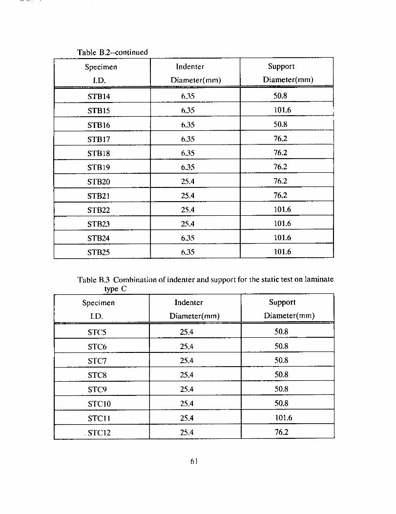
Table B.2--continued

Specimen

I.D.i

STB14

Indenter

Diameter(ram)

Support

Diameter(mm)

6.35 50.8

STB15 6.35 101.6

STB16 6.35 50.8

STB 17 6.35 76.2

STB 18 6.35 76.2

STB19 6.35 76.2

STB20 25.4 76.2

STB21 25.4 76.2

STB22 25.4 101.6

S'FB23 25.4 101.6

STB24 6.35 101.6

STB25 6.35 101.6

Table B.3

type C

Specimen

I.D.

STC5

STC6

STC7

STC8

STC9

Combination of indenter and support for the static test on laminate

STC 10

STC11 25.4 101.6

• STC12 25.4 76.2

Indenter Support

Diameter(ram) Diameter(mm)

25.4 50.8

25.4 50.8

25.4 50.8

25.4 50.8

25.4 50.8

25.4 50.8

61

"FableB.3--continued

Specimen Indenter Support

I.D. Diameter(ram) Diameter(ram)

STC13 6.35 50.8

STC14 6.35 50.8

STCI5 6.35 101.6

STC16 6.35 50.8

STC17 6.35 76.2

STC18 6.35 76.2

STC19 6.35 76.2

STC20 25.4 76.2

STC21 25.4 76.2

STC22 25.4 101.6

STC23 25.4 101.6

STC24 6.35 101.6

STC25 6.35 101.6

62

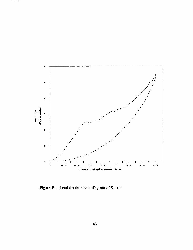
I

I

3.2

Figure B.1 Load-displacement diagram of STA11

t_3

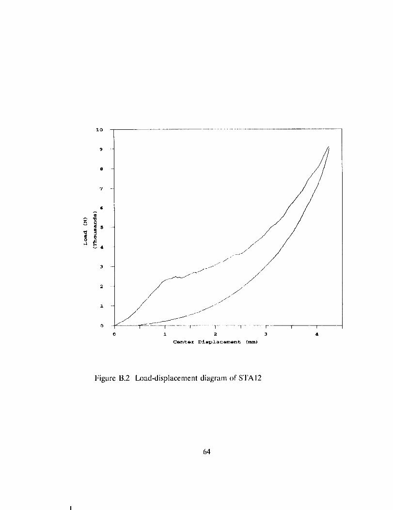
10

7

o

J

-- / j/J'_

_-------"l_-=------r- ------_ .... -r- .... 1

0 1 2

r i i

3 ll

Ceziter Displacement (mm)


64

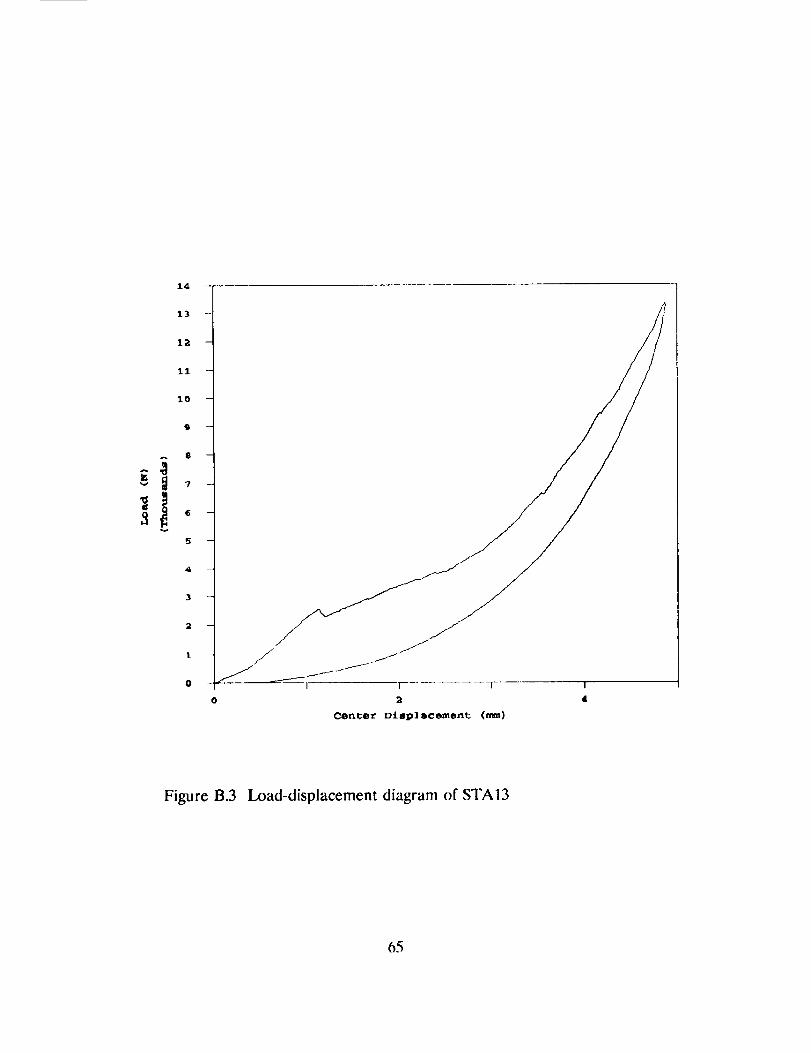
14

Figure B.3 I.x)ad-displacement diagram of STAI3

65

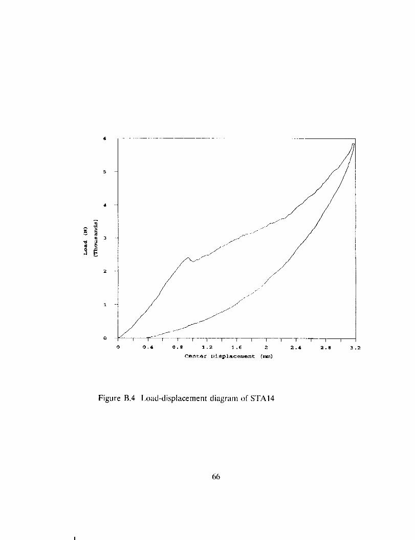
Center Displacement (nm_)

Figure B.4 h)ad-displacement diagram of STA14

66

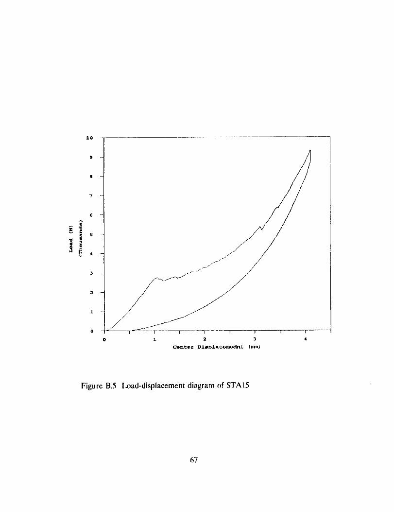
lo

7 -

6 -

•rJ m

v

2

.f /

/., ,J*

I 1 I

0 1 2 3 4

Cente_ Diaplacomoch_t (turn)

Figure B.5 l_x)ad-displacement diagram of STA15

67

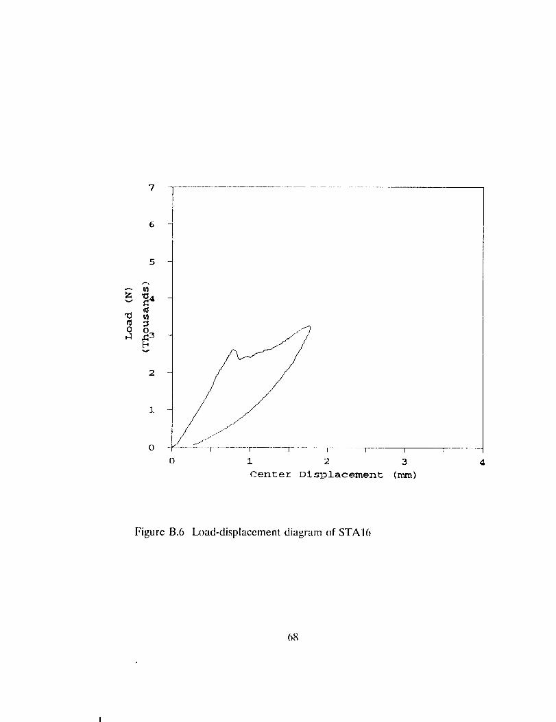
7

6

5

v

0

v

2

1

........... I T I i I I

1 2 3

Center Displacement (nun)

4

Figure B.6 _)ad-displacement diagram of STAI6

_8

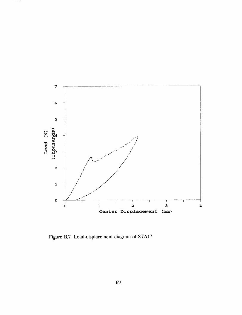
7 -

5 -

Z _4 -v

0

v

2

1

0

///

/_//

| I I

1 2 3


4

Figure B.7 I_xmd-displacement diagram of STA17

69

7 ........................

6 --

5 -

Z _4 -v

m0,-.]._3 --

2 _

l 2 3

Cente_ Displacement (mm)

4


70

7

6

5

•.-- ta

z _4

0

2

1

I I i I I !

O 1 2 3

Center Displacement (m)

4

Figure B.9 Load-displacement diagram of STAI9

71

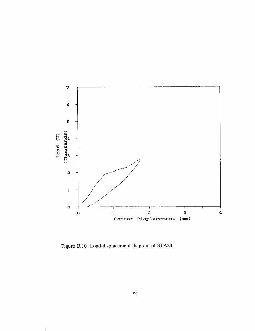
7

6 -

5

z _4v

o _3

1

o I T [ F- I I

1 2 3


4


72

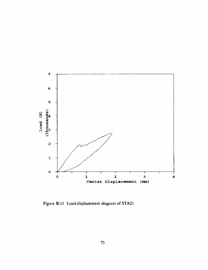
7

6

5 -

•"-- t/l

Z _4 -v

'_ ca

o ._3

2

1

0

0

I I ! ! !

1 2 3


4


73

7

6

--- m

v

mm

023

v

2

0i I I I f I 1

0 1 2 3


4

Figure B.12 Lx)ad-displacement diagram of STA22

74

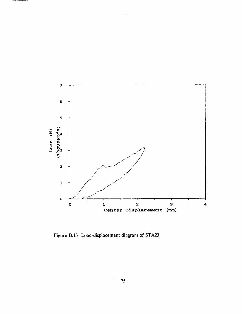
7

6

5

zv

"0 ta

0

v

2

O

O

I I I I I

1 2 3

Center Displacement (nan)

4


75

7

6 -

5 -

-"- m

Z _4 -v

ra

0

v

2

1

I 1 I T I I

0 1 2 3


4


76

7

6

5

A

zval

•_1 ta

o

v

2

0

! ! I | I

1 2 3


4


77

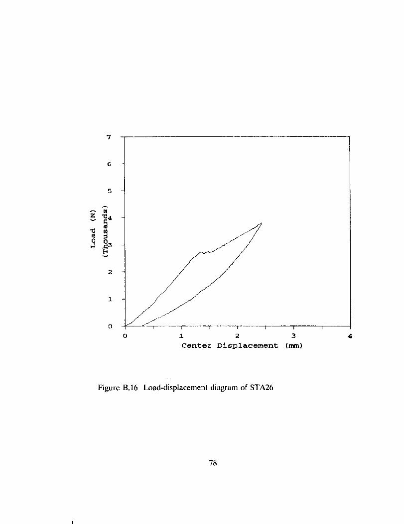
7

6

5

zv

mo

v

2

1

0 I | 1 I I I

0 1 2 3

Center Displacement (n_n)

4


78

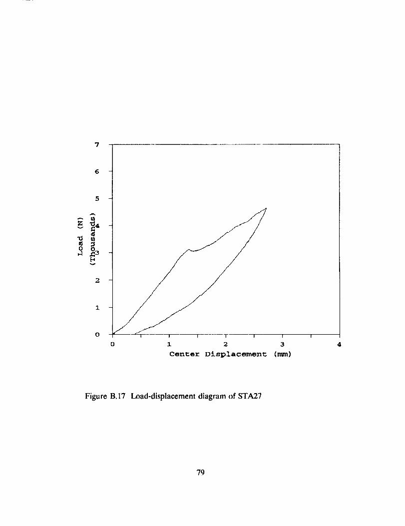
7

6

5

]!.2

1

! ! ! ( !

0 1 2

Center Displacement

I

3

(m)


79

7

6

z _4v

ta

o _3

1

0 ! I I I | I

0 1 2 3


Figure B.18 l_x)ad-displacement diagram of STA28

80

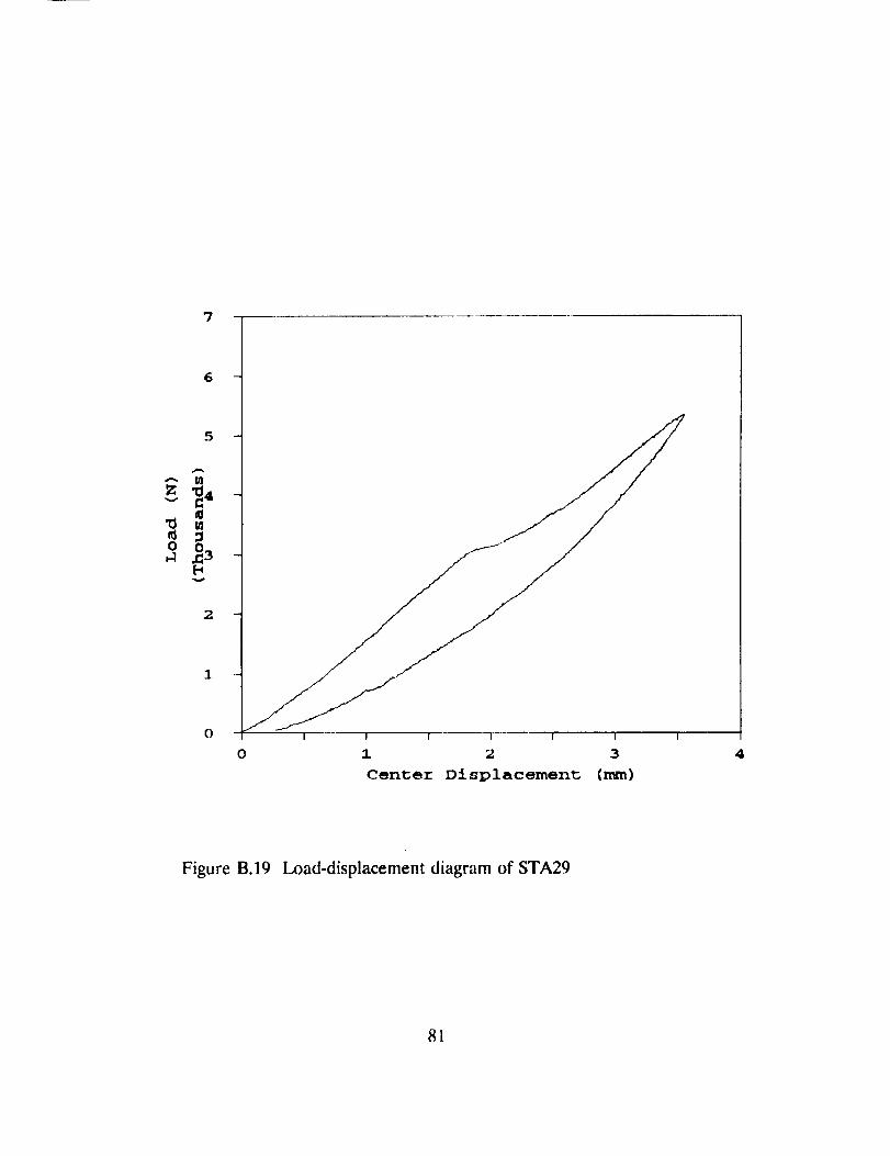
7

Ill

_3

v

2

1

0

0

I I I I I

I 2 3


4


81

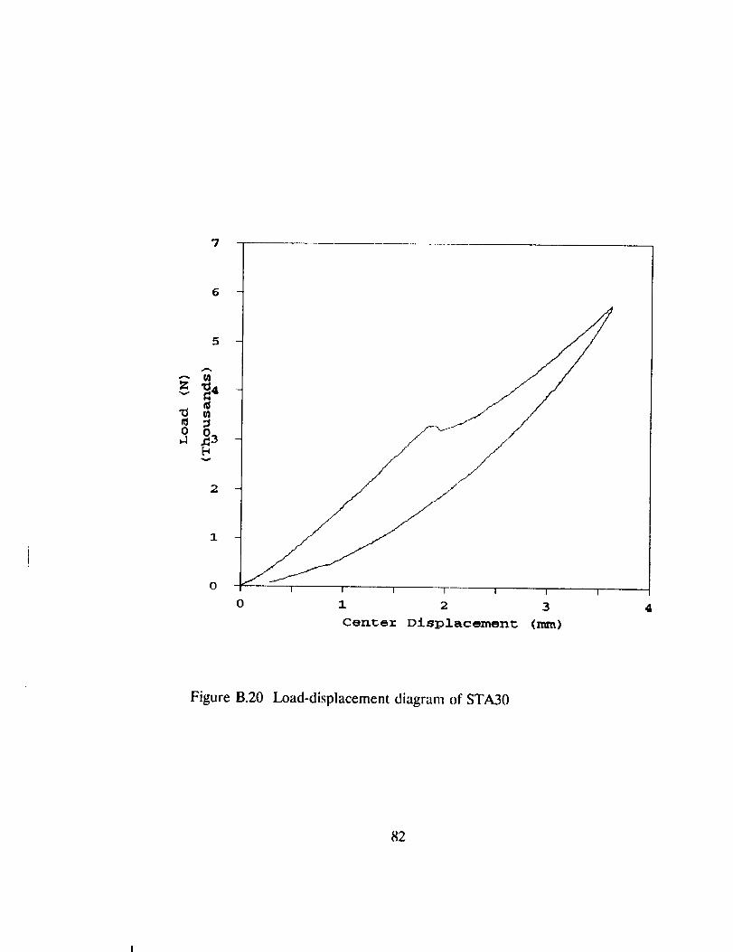
7

A

v

0

v

2

1

0I I I I I

1 2 3


4


82

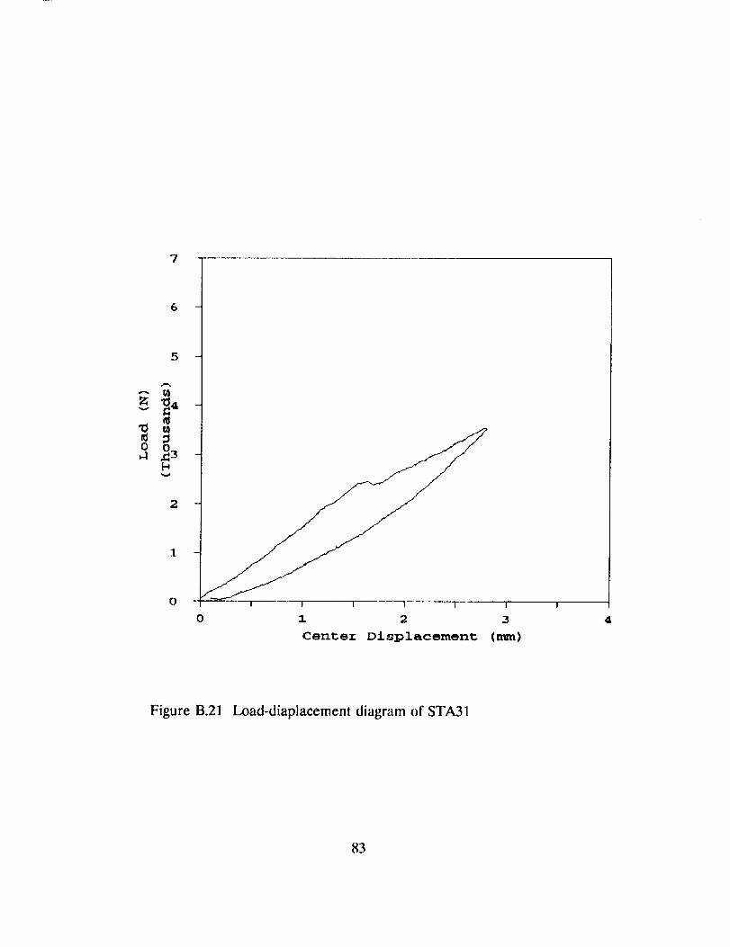
7

6

5

--- t_

z

0

v

2

1

0 i l l l I i i

0 i 2 3

Center Displacement (r_n)

4

Figure B.21 Load-diaplacement diagram of STA31

83

7

6 -

,.,5

2

1

o iI I I I I

0 1 2

Centor Displacement

I

4


84

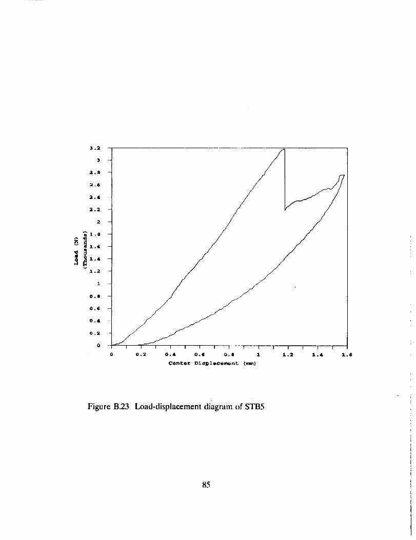
3.2

3

_3.8

2.6

;t.4

2.2

2

ml.8

1.2

1

0.8

Oo&

0!

1.4

Figure B.23 Load-displacement diagram of STB5

85

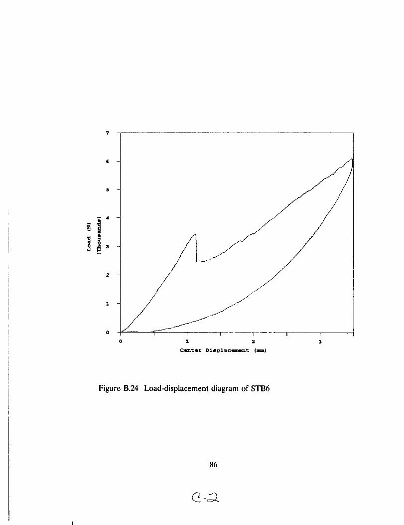
4

Q


86

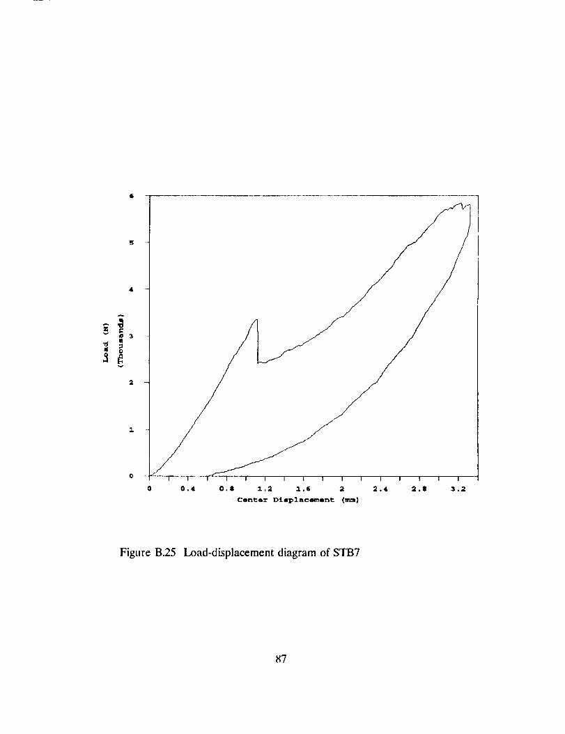
6

w.v 3

II

It 0

v

0 O.4 0.8

I

2.8


87

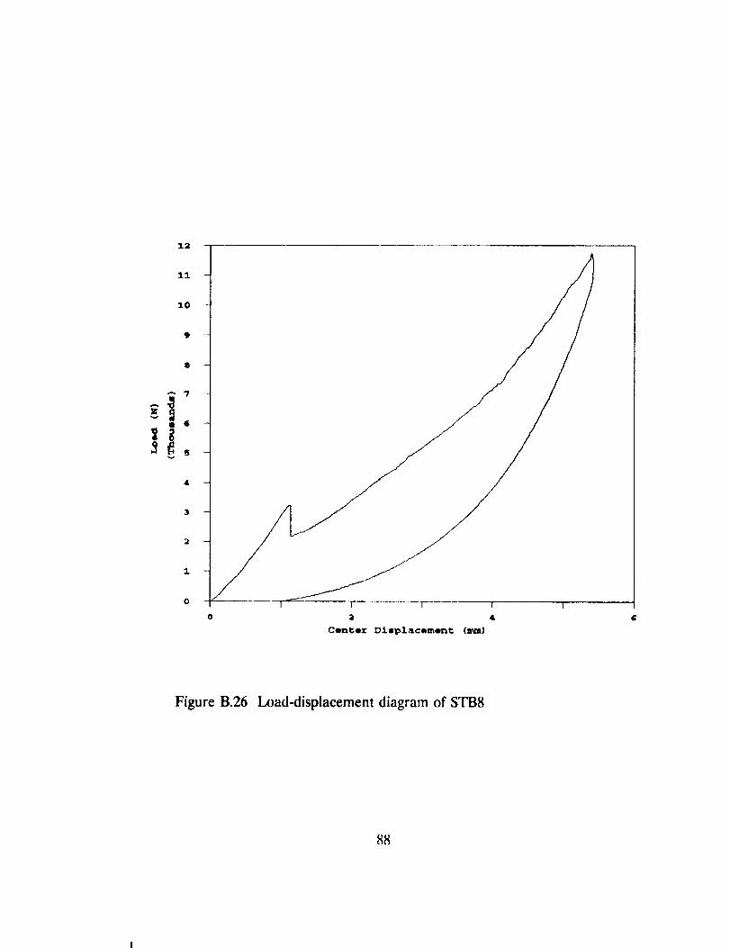
12

13.

10

9

8

v

3

2

1

0


88

7

6

5

ttl

zvm

o

2

1

0 [ I I 1 I !

0 1 2 3

Center Displacement (rc_)

4


89

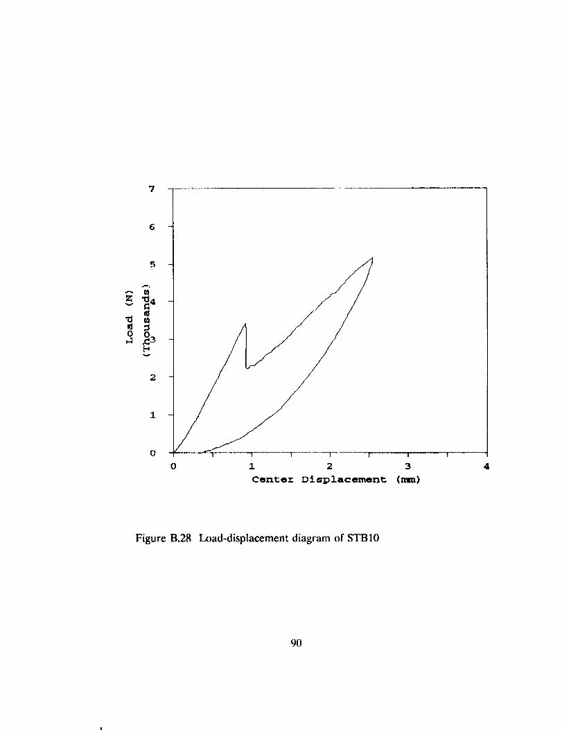
7

6

o _3

2

0

I I I I ]

1 2 3


4


90

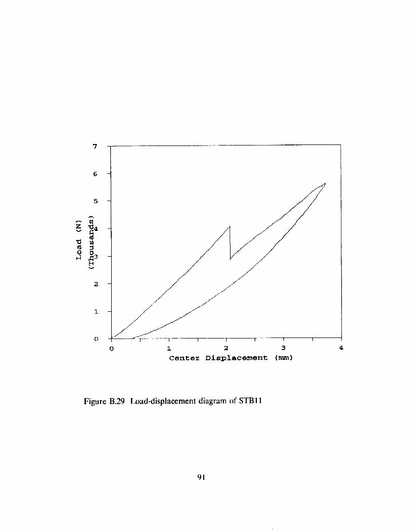
7

6

5

v

o _3

2

1

0 I I I I 1

1 2 3

Center Displacement (ram)

4

Figure B.29 Load-displacement diagram of STBll

91

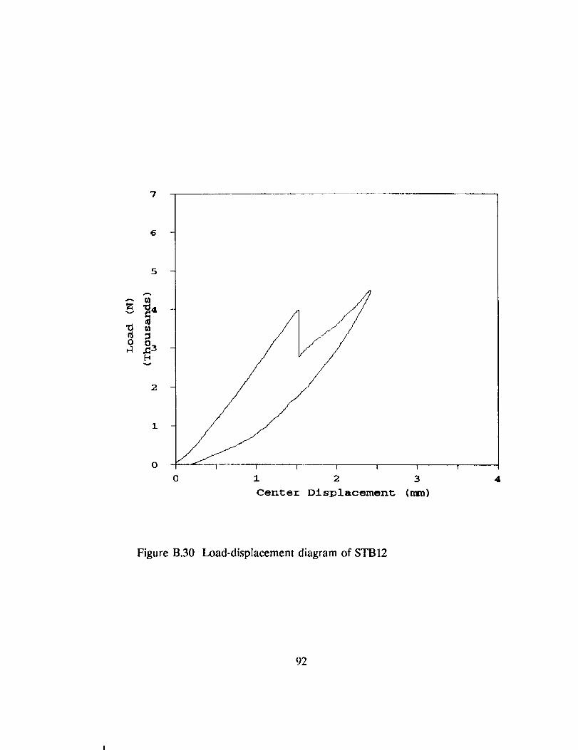
7

6 -

s

2

1

0

0

1 I I 1 I

1 2

Cen_er Displacement

I

3

(mr.)

4


92

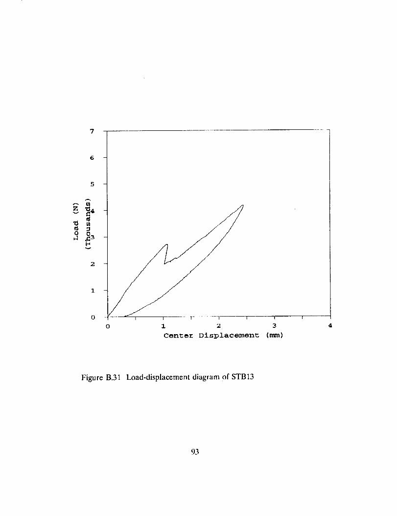
7

6 -

5 -

z _4m

0

2

0

I I I ! !

1 2 3

Cen_er Displacement (mm)

I

4


93

7

6 -

5 -

v

t_

3H

2

1

0 i ! I I ! I i

1 2 3


4

Figure B.32 Load-displacement diagram of STBI4

94

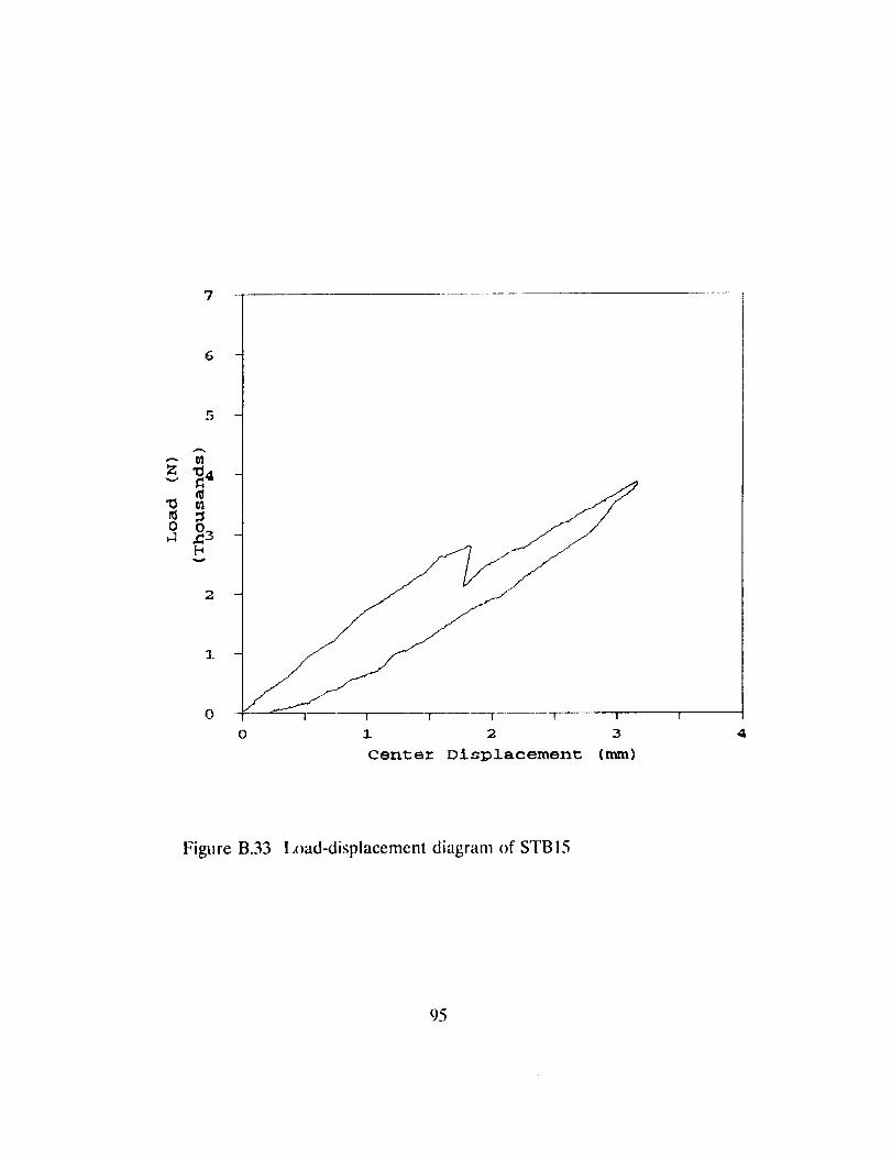
7

G --

5 --

V

aJa3

o

9.

1_

o I I [ I I

1 2 3


4

Figure B.33 l_x_ad-displacement diagram of STB15

95

7

6

xl mr4

o _3

2

I

0

0

I 1 I t I

1 2 3

Center Displacement (_)

4


96

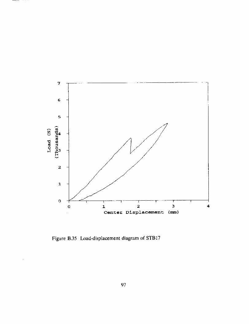
7 - ~ -.!

6 -

5 -

zv

0

2

1

0 1 I I i "1"

0 1 2 3


I

4


97

7

6 -

,_,5

2

1

0

0

[ | I t I

1 2

Center Displacement

I

3

(mm)


98

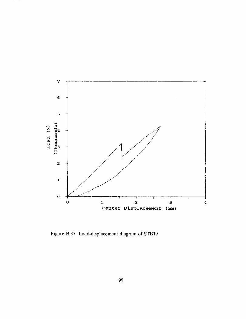
7

5

--- ta

z _4v

"0 ta

o

v

l I I T i

o 1 2 3


4


99

7

6

5

,-. ta

"0 ta

o _

v

2

0

0

I I I I I

I 2 3


4

Figure B.38 .Load-displacement diagram of STB20

100

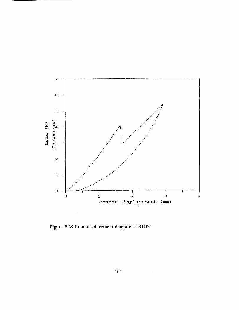
'7

6

5

v

0

v

2

O

t

o 4

Figure B.39 l_x)ad-displacement diagram of STB21

101

7

6

z _av

"0 ta

o _3

2

1

0I ! I I I ! I I

0 1 2 3


4

Figure B.40 l.xmd-displacement diagram of STB22

102

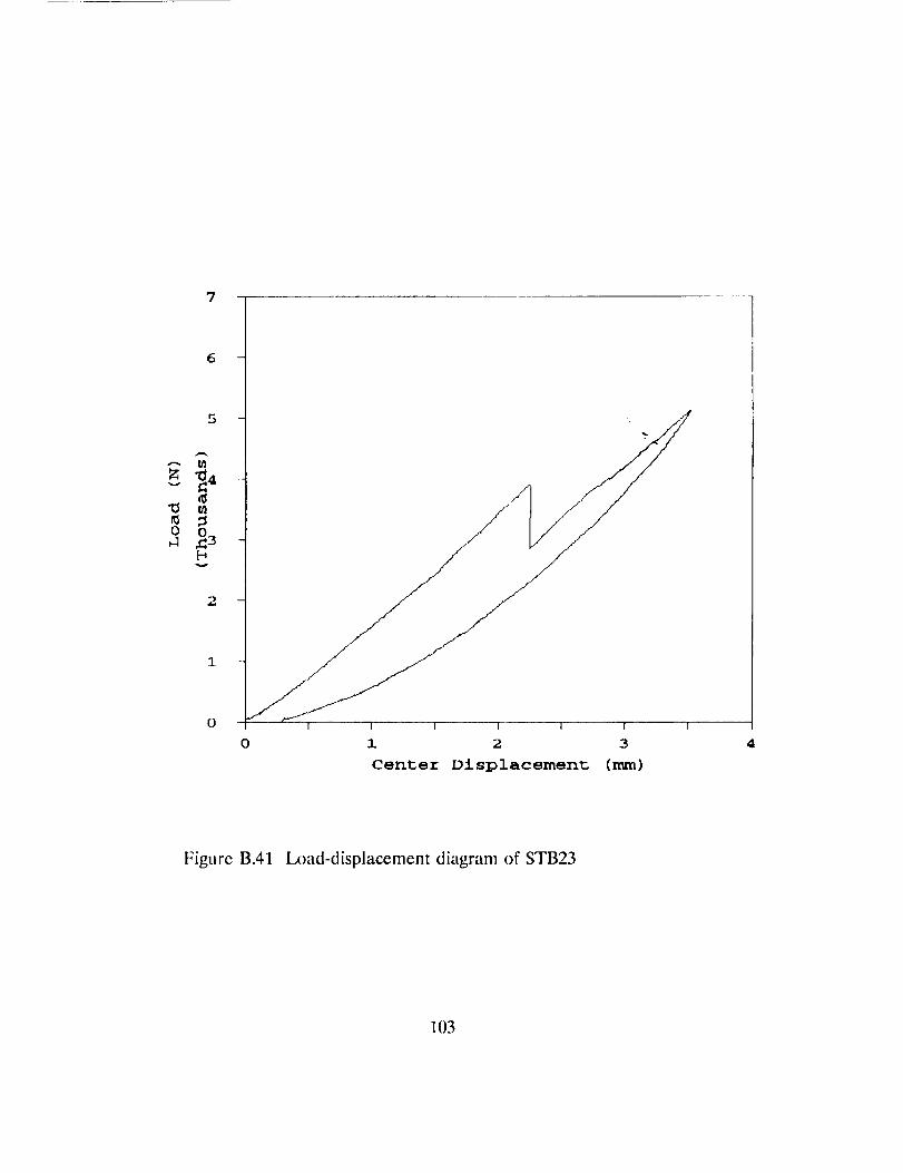
7

6 -

5 -

zv

0 _

v

2

1

I I 1 I i ( I

o 1 2 3


4


103

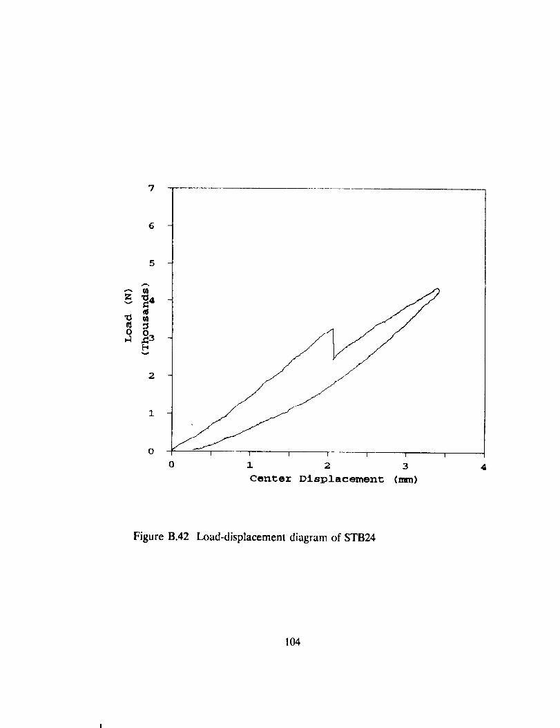
7

6

5

-_ tA

,1::3

v

9.

1

0I I ! I I f

0 i 2 3


4


104

6 -

5

zv

O

v

2 --

1 -

o

o

I I I I I I 1

1 2 3

Center Displacement (_)

Figure B.43 l_xmd-displacement diagram of STB25

105

3.S

2.5

i 2

1,5

/

0.5

Figure B.44 Load-displacement diagram of STC5

1()6

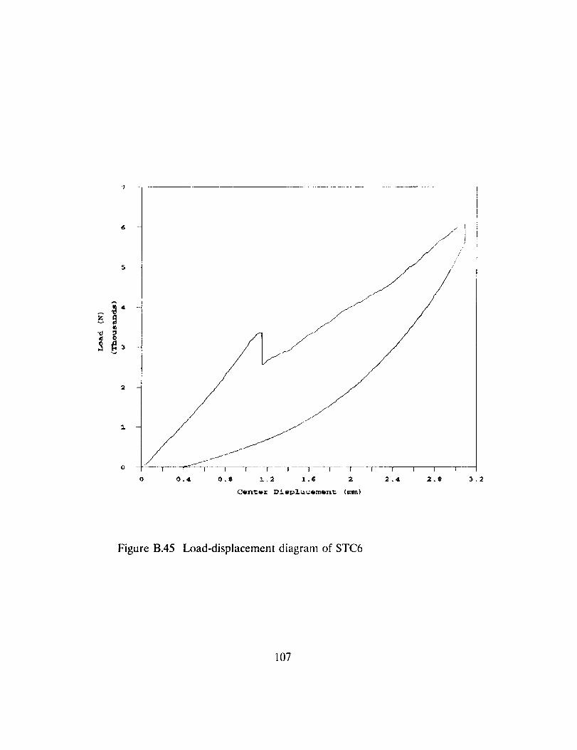
la

v

0.4 O.S

/

//

/

I ---T--V----_---T-- ]-- ! . I I I 3

1.2 1._ 2 2.4 2._

C@n_uz Displac@_nt (mm)

3.2


107

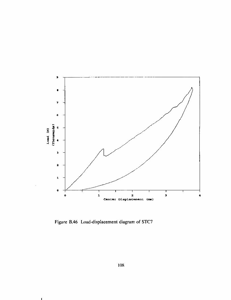
9 -

8 -

7 -

.._5 -

v

2 --

i 2

csn_sr Dieplacemenh (_e_)

Figure B.46 l_x_ad-displacement diagram of STC7

108

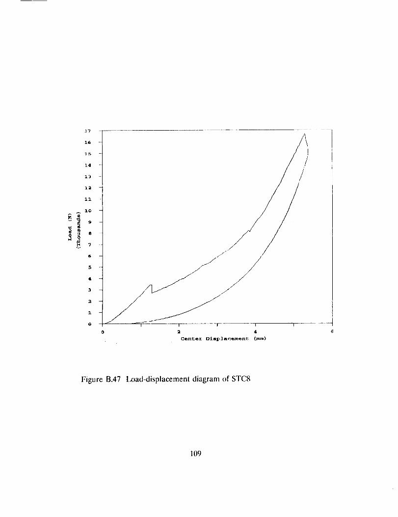
17

16

15

14

13

12

II

i0

_ 9

_ 7

6

5

4

2

0


109

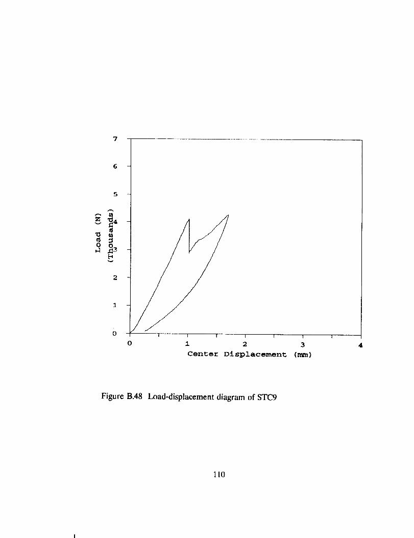
7 -

5

2

3_

Oi I I I I T

O 1 2 3

Center Displacement (n_m)

!

4


110

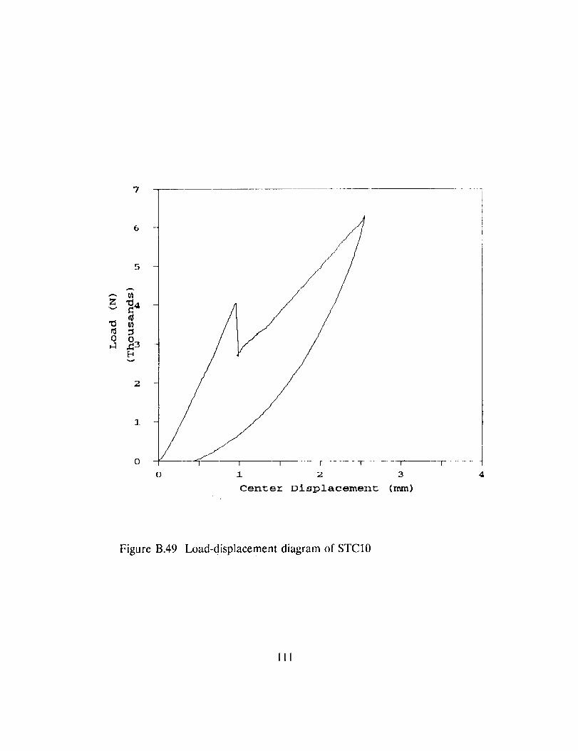
7

6

z _4

0

2

0

1 I ........ f T i

1 2 3


4

Figure B.49 Load-displacement diagram of STCIO

111

7

6

5

A

m

zv

0

v

2

/.

o

0

I I I l I

1 2 3


Figure B.50 l_xmd-displacement diagram of STCI 1

112

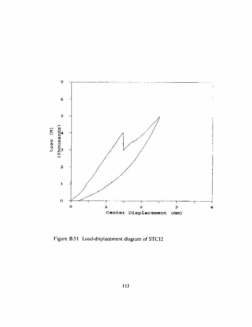
7 --

6 -

5

zv

mm0

v

2

1

T T i [ l

l 2 3

Centez Displacement (mm)

I

4

Figure B.51 l_xmd-displacement diagram of STC12

113

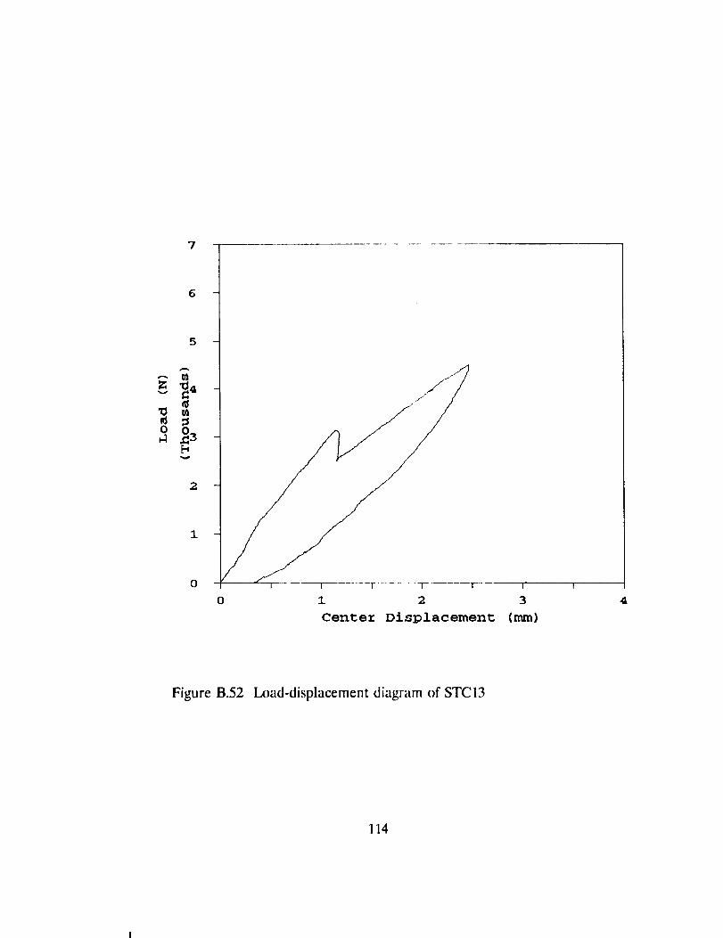
7

6 -

5 -

-"- 51

v

m

o

2

1

0 I I T 1 !

0 1 2 3


4

Figure B.52 Load-displacement diagram of STCl3

114

7

6

5

v

al

o

v

2

1

1 I I F- I

o 1 2 3


4

Figure B.53 Load-displacement diagram of STCI4

115

7

6

--- ta

v

o

2

1

0I I I [ I 1 I

0 1 2 3


4

Figure B.54 Load-displacement diagram of STC)5

116

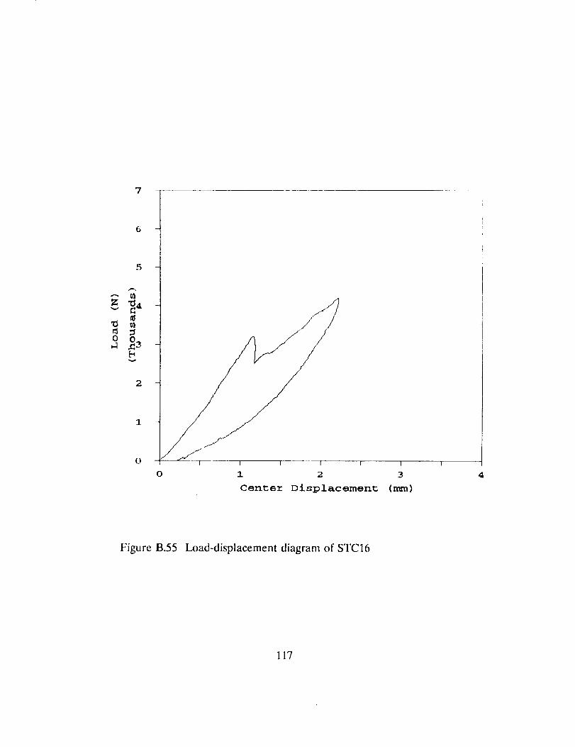
7

6 -

5 -

Z _4 -v

° 23v

2

I

0

0

! [ l

1 2 3


4

Figure B.55 I.x)ad-displacement diagram of STC16

117

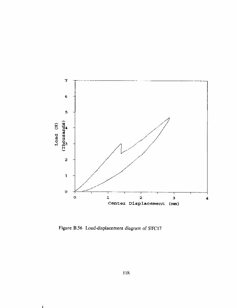
7

6

5

•-- t_

z _4v

ta

0

v

9

1

O

_ //

/

1 I I I I

0 1 2 3


4

Figure B.56 l_x)ad-displacement diagram of STC17

118

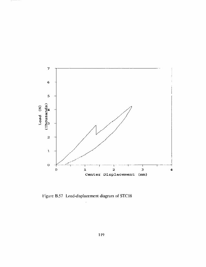
7

6

5

z _4

0

2

1

0

/

T 1 I 1 I

o l 2 3

Centez Displacement (mm)

Figure B.57 Load-displacement diagram of STCI8

119

7

6

5

•--- th

z _4V

mo,a _3

v

2

1

I I 1- I i

0 l 2 3

Cente_ Displacement (ram)

4

Figure B.58 l_xmd-displacement diagram of STC19

120

7

6

5

z _4v

0

v

2

1

0 I I T I

l 2 3



12!

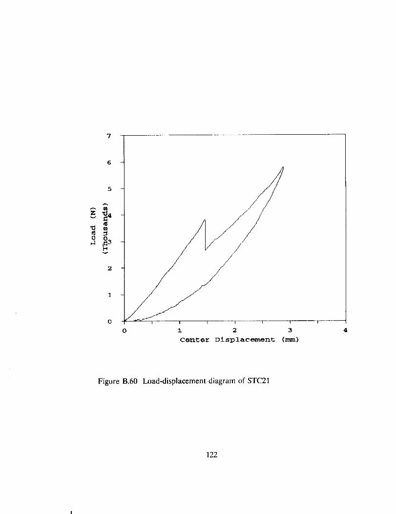
5

z _4

0

2

1

0

0

I I I t

1 2 3

Cen_er Displacement (nun)

4

Figure B.60 l_x)ad-displacement diagram of STC21

122

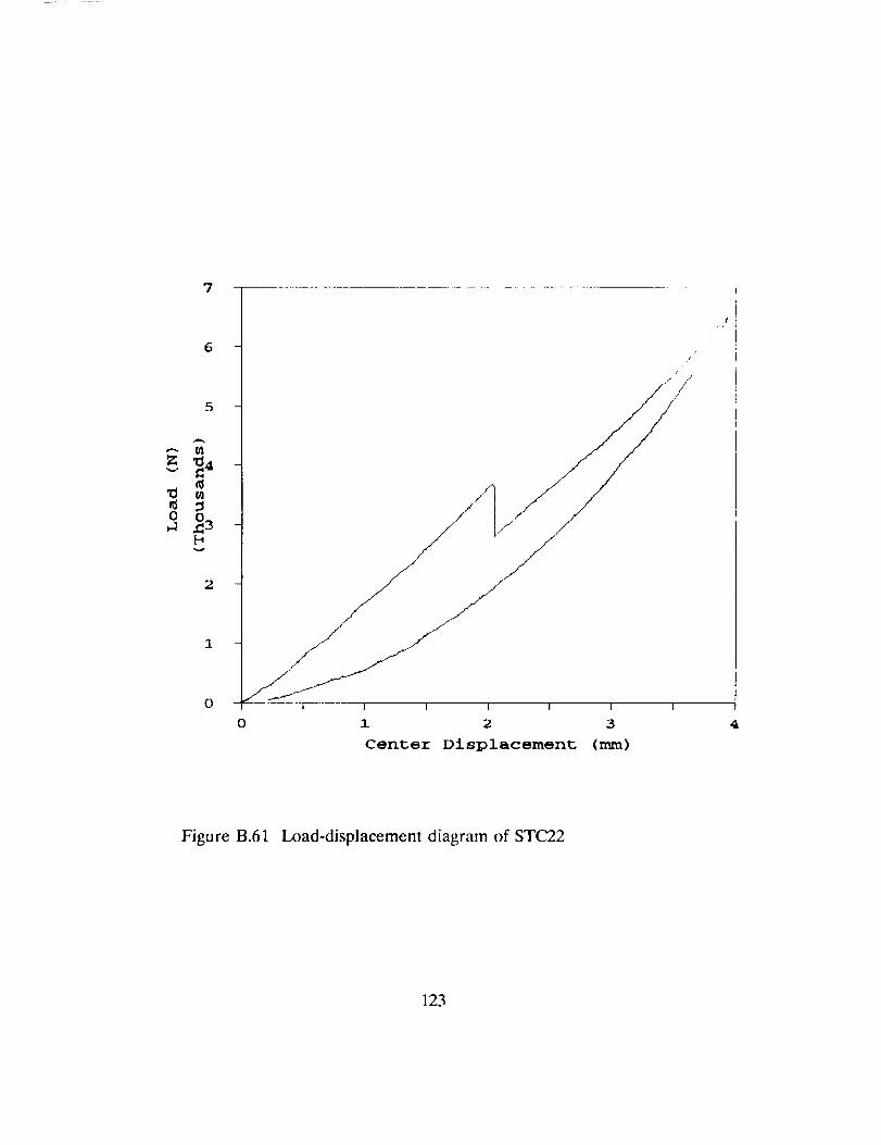
7

6 -

5

Z _4 -v

0._3 -

v

2 --

1 --

0

o

/

/

/

I I I I ! l I

1 2 3


. /

4


123

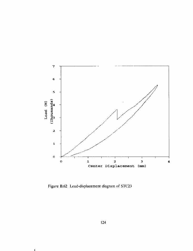
7

6 -

5 -

rh

Z _4 -v

a_-o t_mo

" /

0 T I I T

//

I I 1

o 1 2 3


4


124

7

5

A t_

z _4v

0

2

1

1 I I [ I I I

1 2 3


4


125

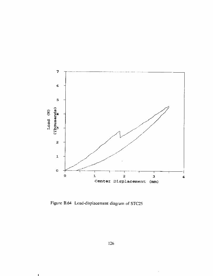
7

6

5

z _4

0

o

/-

I 1 1 1 1 t I

0 l 2 3

Cente_ Displacement (mm)

4

Figure B.64 I_x)ad-displacement diagram of STC25

126

APPENDIX CDATA FOR LOAD-DISPLACEMENT DIAGRAMS

The plate stiffness (KI), the load and the center displacement at the first

obgervable failure (PI and q_ respectively), the load drop at the first observable

f_Jl_He (ziP), and the slope of the yield curve (/(2) for various specimens _tc

pre_ented in this appendix. Figure C.1 is the key for various data presented in Tab!e

C.1.

m

q2: Centel: d..tmlpla.¢omont: at: P3

Klt gecant: moCtxtluls (P1/q!)

X2t Jlopo of y£eld ©_ve

(pa - t,2) / {q.2 - q:3.)

_it/%p

P_t

Cent;or dt mplacqenont

Figure C.I Sketch of typical load-displacement diagram

127

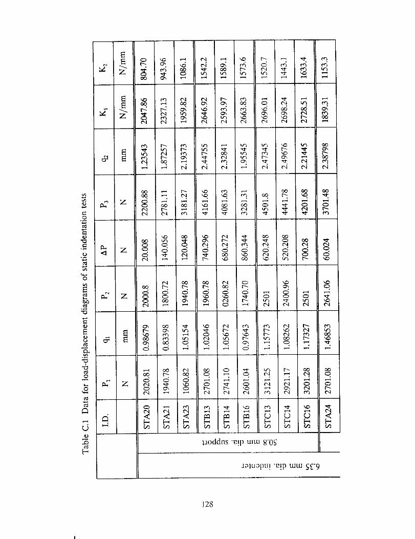
_ I"_ _ _ ',::t" _ _ _

_ e,,i e,i t"-_ ,.--, t'-,i c',,i _ c,,a

<D

0. ,...+

4,.i

00

o.,._.i,-1

0

B

t:m

E0

B

.6©

e"d

,i-.,4

0ca

[....<

<:1

m-

Z

Z

Z

Z

e,I ('4 pea _ _ _ _ ',zl- _

o o _. _ t.<-+ _ cq e,t. t',,ao o <:5 o <::5 o <_ o o o<:5 _ t"q .m'- _ ,,_ e,_ ¢q o

_; ,::5 o o _ _ <::5 _

C'q _ _ ,---+ _ _ t",l t",l _ t',l

oo _ _ 0 '_ t_ t_ oO_0 I_ _ _ ,_ 0 _ _ _.

0 _ _ I'_ P'_ ',0 _ <2", ¢'4 I'_

i

1J0ddns "e.!p mtu g'Og

.Ialuapu! "e.!p tuu.t _;_'9

128

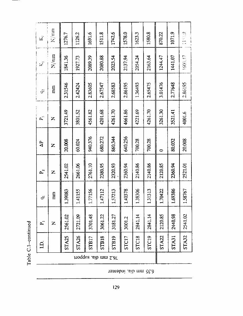
E

Z

'r .... "-'T-- ---"*

Z

t'-.- t",,I O', ,-.-* "_- t"_ ¢',1 oO _:D t _¢,q _ _,_ _ I"_ _ ,,_ _ t"..

E_

I_ _' Z

u")x,-,,l

¢,q

¢.q

oo

2:0

¢,q0

,=5

Z

oo oo

i,-,-I

¢,q

ooI,-,,I

,r,-,l

¢,,q

Cq

EE

¢)

-f.,4

0?I

d¢)

,.£::)

Z

°

1Joddns "e!p mm E'9L

aOlu_ptl.1. "e!p tutu _£'9

129

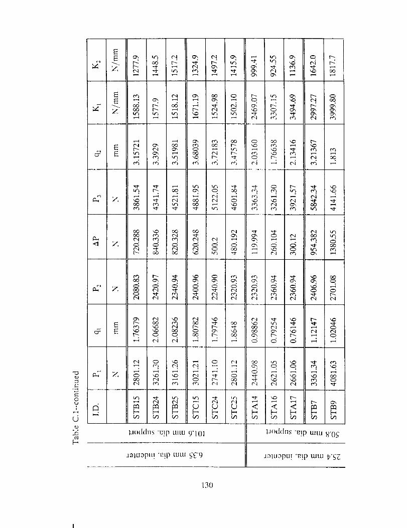
E_-_ cm _ I_-

un _ e,i

¢"4 _ '_ 00

cg ¢',I Cm _0 O I_-

_- CO I_- _ I_- C-I O

EE

_ O,l O0.,._.;

_ c'q oo 1"4 0cq _ oo

Z

O0 ",,0 O0 O0 t"q

0,1 "Lt" t"q _ 0 oO{"-I _ 0",

Z

I_- _ ',o _ _ c_0o o _, o', _ o', o', _,

C-I ¢"1 ¢N ¢N C',I ¢q e-I c,I e,,I 04 o,I

E

t'- 0 0 O0 17-- CO 0",

O

ii

d

,.D

d

Z

C,,i 0 _ _ 0 r-,l oo

61 _ rq o'_ nl cq _q

['-, ['-', F-.,

',,.0 ',_ _ 0¢"-1 o,I ¢_

'¢D !'--

•< <

lJoddns "_:]p mtu 9"101

._luoptt! "v.!p tuu_ _£9

1.mddns "_!p tutu R.()_-

Jmuopu! "p.!p tutu _'_;E

130

0'_ _ I"_ _

z _ _ _ _ _

_,_ 0 I"_ _

t"_ _ 0"_

ZoO _ _ 0

C_l 0 _, oO _ _,

Z

oO _ _'_ ',_

Zoo .,_ ,._ o o. _ ,..4 _ ,4

0 c_ _ 0 oO _'_

o_._

0

?!

d

I'_ "_" "_" _1

0 0",

1Joddns "e!p tutu 8"Og

e,4 eq _ r--. ,_. ,_

0

l_oddns "_!p tmu T9L

.laluapu.l "e!p tuw _'S;?;

131

Z

E

Z

<1 Z

Z

_ !"_ _ _ _I_

_:_ _ I_" ¢N _,I'_ _ _ _ ,--_ .,_

c-.i c-i c.i _ c.,i c-i

°_

0

Y.¢....I

0

F_

¢'-,I _ c'-I Pq M::) _ I"_ _

•_ _ _ ,--; ,-1 ,--;

lloddns "P!p tutu 9"IOI

Jaluaput. "e!p mm l_'gg

132

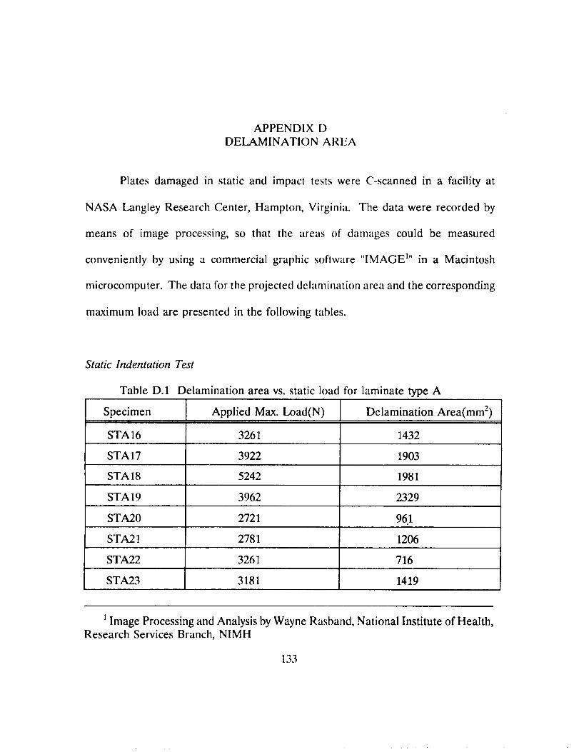
APPENDIX D

DELAMINATION AREA

Plates damaged in static and impact tests were C-scanned in a facility at

NASA Langley Research Center, Hampton, Virginia. The data were recorded by

means of image processing, so that the areas of damages could be measured

conveniently by using a commercial graphic software "IMAGE TM in a Macintosh

microcomputer. The data for the projected delamination area and the corresponding

maximum load are presented in the following tables.

Static Indentation Test

Table D.1 Delamination area vs. static load for laminate type A

Specimen Applied Max. Load(N) Delamination Area(mm 2)m

STA 16 3261 1432

STA 17 3922 1903

STA 18 5242 1981

STA 19 3962 2329

STA20 2721 961

STA21 2781 1206

STA22 326I 716

STA23 3181 1419

n Image Processing and Analysis by Wayne Rasband, National Institute of Health,

Research Services Branch, NIMH

133

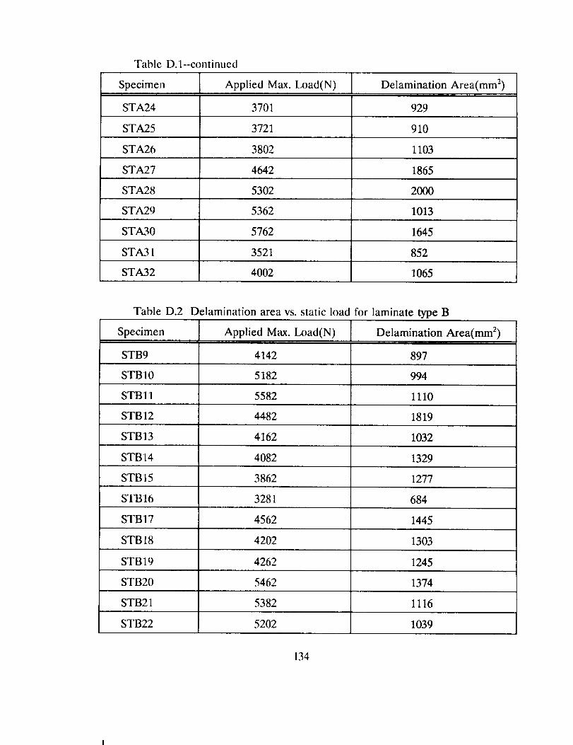
Table D.1--continued

Specimen Applied Max. l_x)ad(N) Delamination Area(mm2)

STA24 3701 929

STA25 3721 910

STA26 3802 1103

STA27 4642 1865

STA28 5302 2000

STA29 5362 1013

STA30 5762 1645

STA31 3521 852

STA32 4002 1065

Table D.2 Delamination area vs. static load for laminate type B

Specimen Applied Max. l_x)ad(N) Delamination Area(mm2)i

STB9 4142 897

STB 10 5182 994

STB 11 5582 1110

STB12 4482 1819

STB13 4162 1032

STB14 4082 1329

STB15 3862 1277

STB16 3281 684

STBI 7 4562 1445

STB 18 4202 1303

STB 19 4262 1245

STB20 5462 1374

STB21 5382 1116

STB22 5202 1039

134

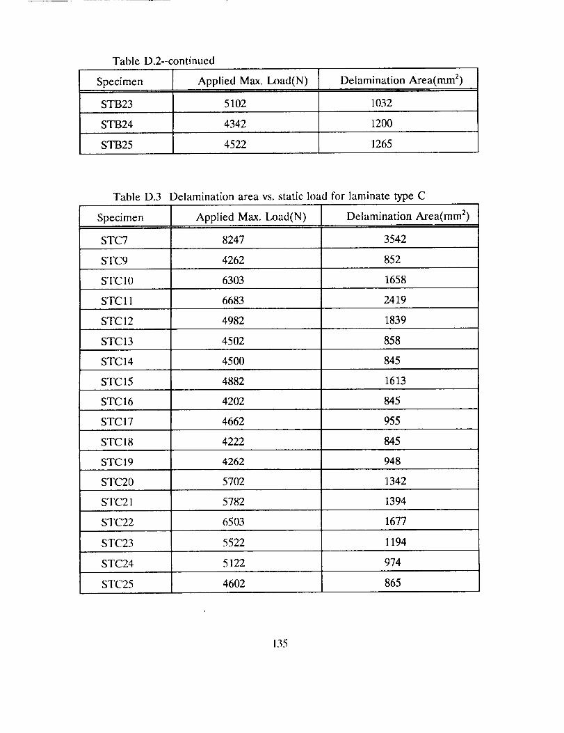
Table D.2--continued

Specimen Applied Max. l_x)ad(N) Delamination Area(mmz)i

STB23 5102 1032

STB24 4342 1200

STB25 4522 1265

Table D.3 Delamination area vs. static load for laminate type C

Specimen

STC7

STC9

STC10

STC 11

STC12

STC13

STC14

Applied Max. Load(N)

8247

4262

6303

6683

4982

4502

4500

Delamination Area(mm 2)

3542

852

1658

2419

1839

858

845

STC15 4882 1613

STC16 4202 845

STC 17 4662 955

STC18 4222 845

STC19 4262 948

STC20 5702 1342

STC21 5782 1394

STC22 6503 1677

STC23 5522 1194

STC24 5122 974

STC25 4602 865

135

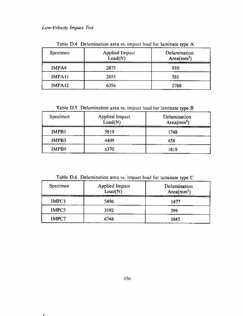
Low-Velocity Impact Test

Table D.4 Delamination area vs. impact load for laminate type A

Specimen Applied Impact Delamination

l_x)ad(N) Area(mm z)

IMPA9 2875 910

IMPAI 1 2855 581

IM PA 12 6356 2768

Table D.5 Delamination area vs. impact load for laminate type B

Specimen Applied Impact Delamination

Load(N) Area(mm 2)i

IMPB1 5819 1748

IMPB3 4409 458

IMPB9 6370 1819

Table D.6 Delamination area vs. impact load for laminate type C

Specimen

i i

IMPCI

Applied Impact

Load(N)'1 i

Delamination

Area(mm 2)

5496 1477

IMPC5 3192 394

IMPC7 6748 1845

136

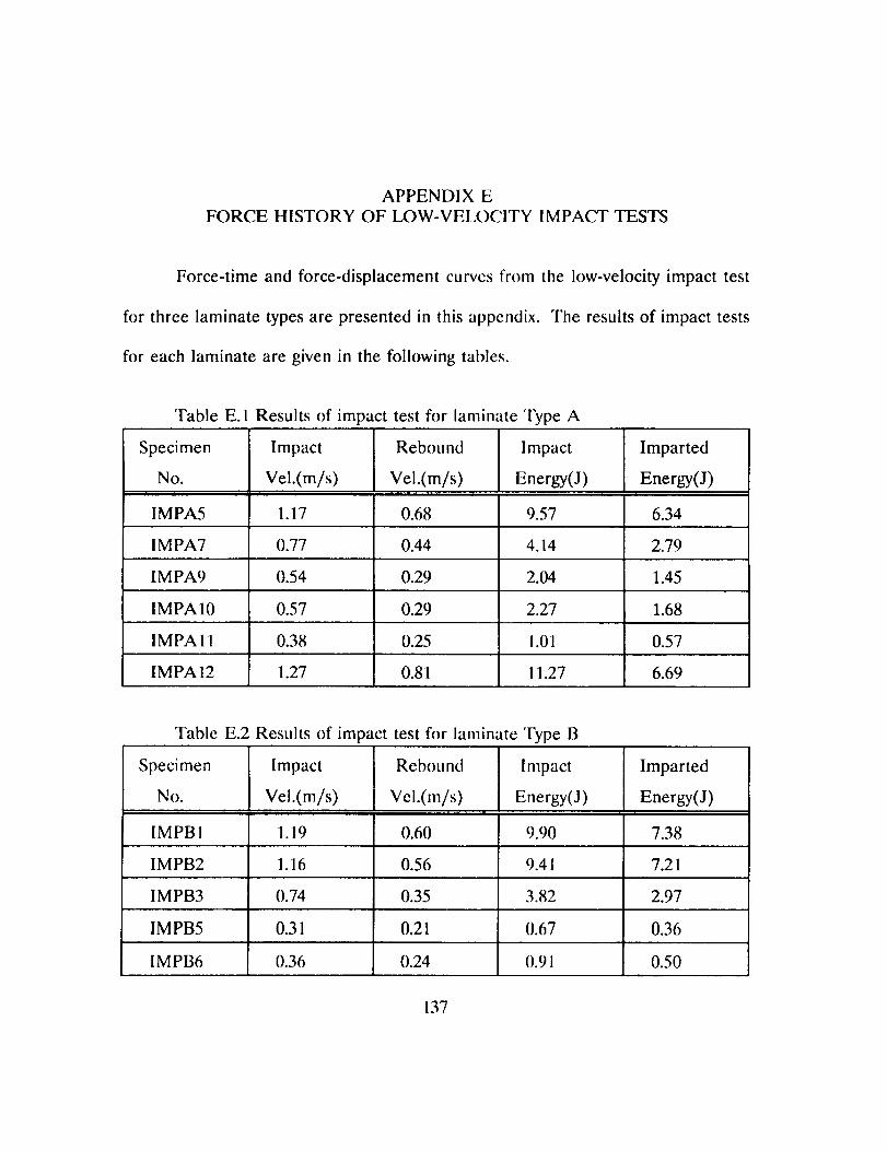
APPENDIX EFORCE HISTORY OF LOW-VELOCITY IMPACT TESTS

Force-time and force-displacementcurvesfrom the low-velocity impact test

for three laminate typesare presentedin this appendix. The resultsof impact tests

for each laminate are given in the following tables.

Table E. Results of impact test fi)r laminate Type A

Specimen Impact Rebound Impact Imparted

No. Vel.(m/s) Vel.(m/s) Energy(J) Energy(J)

IMPA5 1.17 0.68 9.57 6.34

1MPA7 0.77 0.44 4.14 2.79

IM PA9 0.54 0.29 2.04 1.45

IMPA10 0.57 0.29 2.27 1.68

IMPA 11 0.38 0.25 1.01 0.57

IMPA12 1.27 0.81 11.27 6.69

Table E.2 Results of impact test for laminate Type B

Specimen Impact

No. Vel.(m/s)I I i

IMPBI

Rebound

Vel.(m/s)

Impact

Energy(J)

Imparted

Energy(J)

1.19 0.60 9.90 7.38

IMPB2 1.16 0.56 9.41 7.21

I M PB3 0.74 0.35 3.82 2.97

IMPB5 0.31 0.21 0.67 0.36

I M PB6 0.36 0.24 (I.91 0.50

137

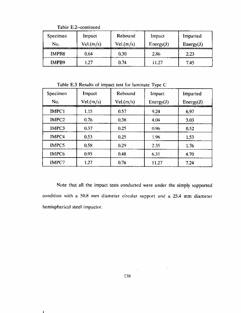
Table E.2--continued



IMPB8 0.64 0.30 2.86 2.23

IMPB9 1.27 0.74 11.27 7.45

Table E.3 Results of impact test for laminate Type C



IMPC1 1.15 0.57 9.24 6.97

IMPC2 0.76 0.38 4.04 3.03

IMPC3 0.37 0.25 0.96 0.52

IMPC4 0.53 0.25 1.96 1.53

IMPC5 0.58 0.29 2.35 1.76

IMPC6 0.95 0.48 6.31 4.70

IMPC7 1.27 0.76 11.27 7.24

Note that all the impact tests conducted were under the simply supported

condition with a 50.8 mm diameter circular support and a 25.4 mm diameter

hemispherical steel impactor.

138

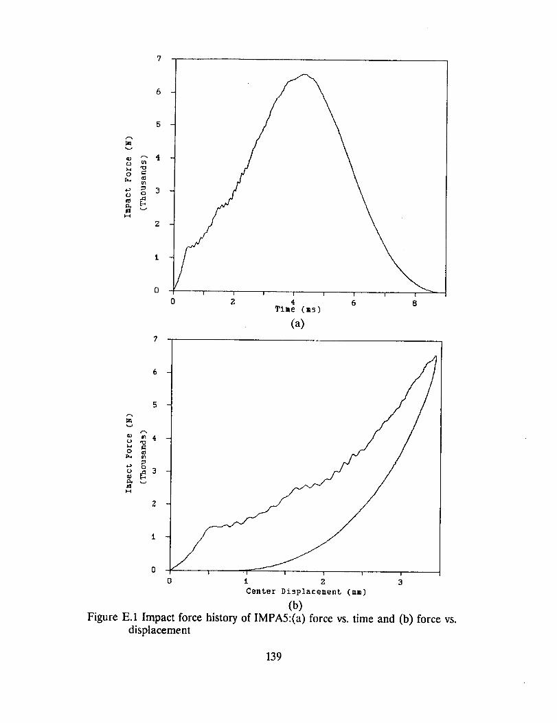
7

I I

5

tJ

0

o _ 30

2

! I i !

4 6Time (ms)

(a)

5

0

Et

1,,,4

! i

I Z


(b)Figure E.1 Impact force history of IMPA5:(a) force vs. time and (b) force vs.

displacement

139

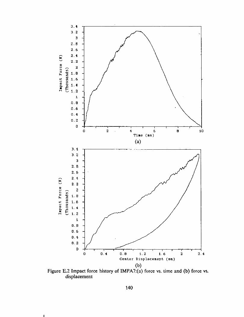
140

O

Or..

O

lak--I

7..8

Z.6

2.4

7..2

,..,1.8

"_1.6¢1(¢1_1.40

_ :1.. 2

0.8

0.6

0.4

0.2

I I

4Time (as)

(a)

g.N¢0

O

m O

H "._

2.8

2.6

2.4

2.2

2

1.8

1.6

1.4

1.2

I

0.8

0.6

0.4

0.2

0 I I I I I I

0.4 0.6 0.8

Center Displacement [mm)

(b)

I

1.2

Figure E.3 Impact force history of IMPA9:(a) force vs. time and (b) force vs.

displacement

141

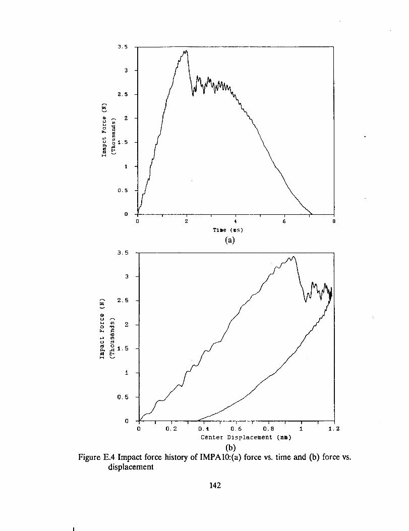
3.5

2.5

1.9

°9

0.5

3.5

! !

Tlme Cms)

(a)

'-" 2.5

+a t_

E-_H

0.5

0.2I I I I

0.4 0.6 0.8

Center Displacement Cmm)

(b)

I

:t

!

1.2

Figure E.4 Impact force history of IMPA10:(a) force vs. time and (b) force vs.

displacement

142

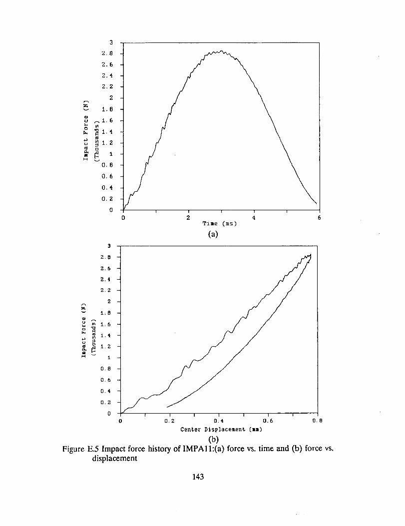
z

U

O

u

elM

2.8

2,6

2,4

2.2

2

1,8

,-, 1. 6

_1.4

0

0.8

0.6

0,4

0,2

0 I I I

2 4Ti_e [ms)

(a)

2.8

Z.6

2.4

2.2

2

"_ 1.8

u m 1 6

2 _ 1.4

I

0.8

0.6

0.4

O.Z

o

0.2! !

O.4 0.6

Center Displacement. (mm)

(b)

0.8

Figure E.5 Impact force history of IMPAlh(a) force vs. time and (b) force vs.

displacement

143

k.d

U

O C0U. ta

U

I I

4 6

(a)

m

o ou

I I I

2

Center Displacement Cram)

(b)Figure E.6 Impact force history of IMPA12:(a) force vs. time and (b) force vs.

displacement

144

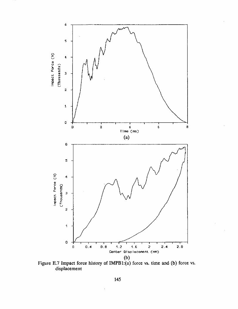
4

U ,",

Is =tt.

3

uI_ 0

2

I I

4

Time Cm6)

(a)

L0U.. C

3

_ 0r'-

2

I ! 1

1.2 I .6 2

Center Dlsp lacement Cram)

(b)Figure E.7 Impact force history of IMPBI:(a) force vs. time and (b) force vs.

displacement

145

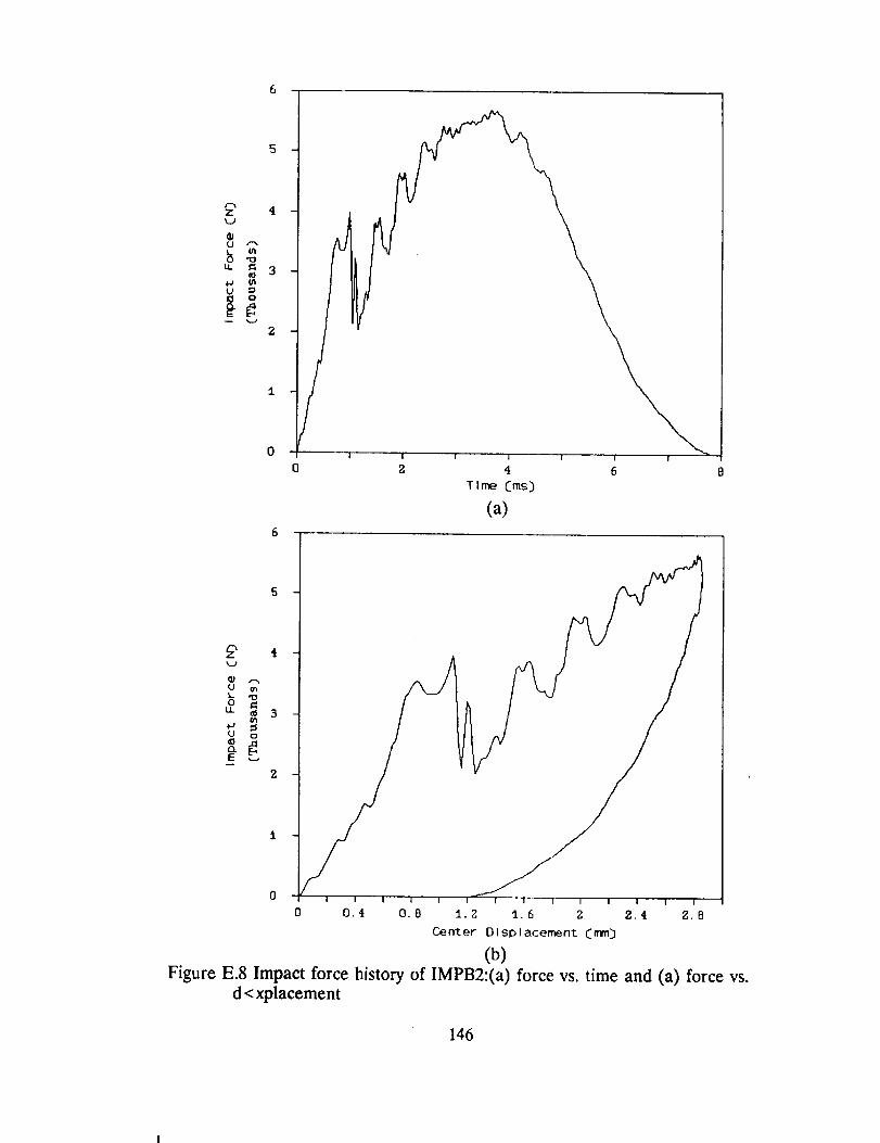
z 4k..,/

U r.x

"33th

U

2

AJ

I

tI

!

!

2 4 6

Time Cms)

(a)

_ 4

0 cn

oLL _ 3

U o

E _

2

Figure E.8 Impact force history of IMPB2:(a) force vs. time and (a) force vs.

d < xplacement

146

4.5

3.S

k.J

U r-.

o _2,5U.

E

I.S

0.5

't.5

i

4

Time Crr6;)

(a)

3,5

z 3

u g'z._L

nII0

0

1.5

0,5

0

0.2 0.4 0.6 0.8 1 1.Z

Center OIsp I_cement Cmm_)

(h)

1.4 1.6 1.8

Figure E.9 Impact force history of IMPB3:(a) force vs. time and (b) force vs.

displacement

147

2

2 2

1 8

z1 6

L _I 40LL

+J _12U

0 8

0 6

0,4

0.2

Z,4

! ! I ! I I

2 4 6TIfT_ _ Cn'_J

(a)

2.2

Z

1,8

z 1.6

u "-'1.4LO

o

0.8

0.6

0.4

O.Z

I I I

0.2 0.4

Center Dlsplacement (ram]

(b)Figure E.10 Impact force history of IMPB5:(a) force vs. time and (b) force vs.

displacement

148

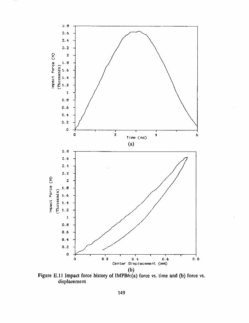
2.8

2.6

2.4

2.2

2

_.8

m

v _1.40

0.8

0.6

0.4

0.2

0

2.B

I I I I

0 2 4Time Crns3

(a)

2.6

2.4

2.2

_' 2

w 1.8

I..o

u_ "_ 1.6

o _1.4

0.8

0.6

0.4

0.2

0 0.2I ! I |

0.4 0.6

Center Olspl acement CmmJ

(b)

0.8

Figure E.11 Impact force history, of IMPB6:(a) force vs. time and (b) force vs.

displacement

149

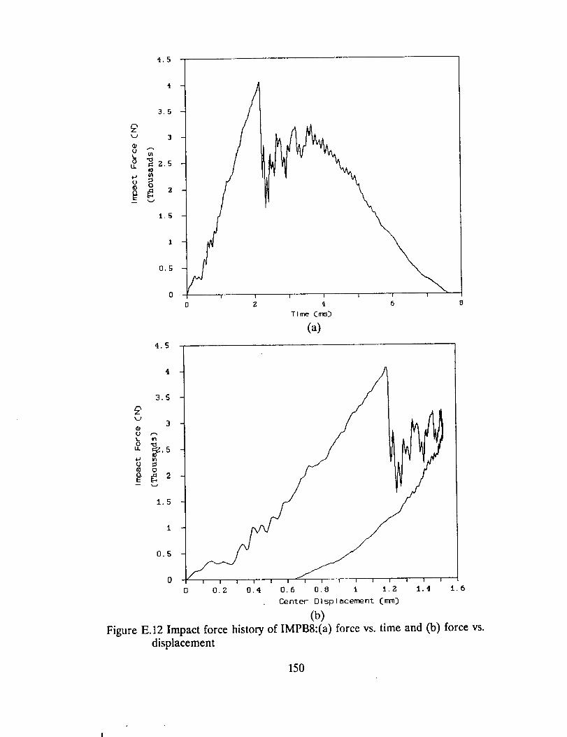
4.5

3.5

3

@

o _25u_

+_o

1.5

0.5

4.5

I I

6

3.5

3

U _

u. .5

o

1.5

0.5

0

0 0.2 0.4 0.6 0.8 1 1.P. 1.4 1.6

Center D I sp I aceme nt C ram)


displacement

150

£

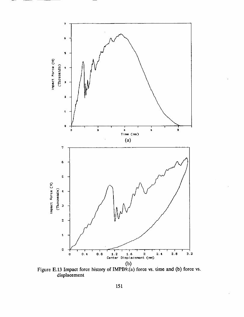
U

4-J 0

I/

/f

I !

0 2

I I I

4 6

Time Cms)

(a)

• _'4

L

O

0

o 0.4 0.8 1.2 1.6 2 2.4 2.8 3.2Center Dlsplncement (ram)


displacement

151

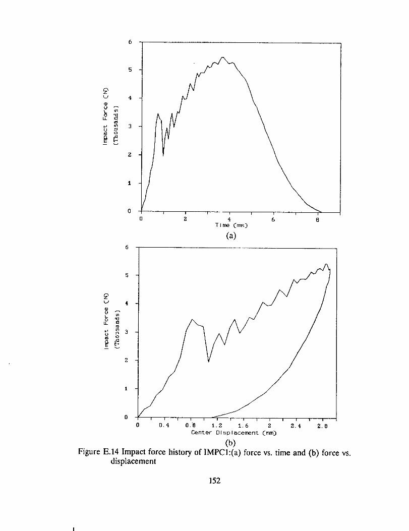
U

t.L¢0

U

/D

| I I I I

2. 4 6Time (ms)

(a)

£_ 4

L _0 '10

0

Figure E.14 Impact force history of IMPCI:(a) force vs. time and (b) force vs.displacement

152

3.5

2.5

_'2$_0 -El

m

.g.s

0,5

3.5

4

Tln_ (ms)

(a)

2.5

Z

L e_0LL

(A

U O

O.F: ""

0.5

0

0 O,?, 0.4 0.6 0.8 I 1.2 1.4 i,6 1.8

Center Olsplacemednt (mm)

(b)Figure E.15 Impact force history of IMPC2:(a) force vs. time and (b) force vs.

displacement

153

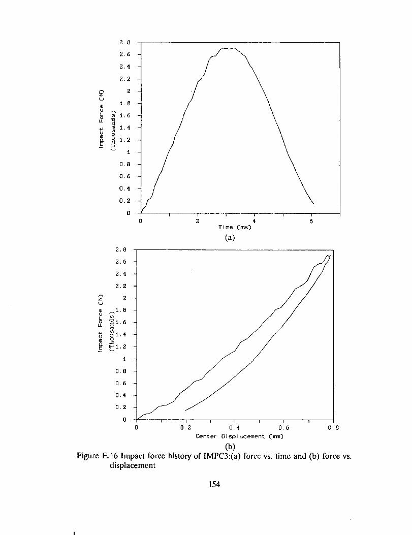
k._t

0L0

LL

2.8

2.6

2.4

2.2

2

m 1.6

_ 1.4

0.8

0.6

0.4

0.2

0

2,6

I i l I i I

Z 1 6Ti me Cn_]

(a)

z

¢J0L0im

2.6

2.4

2.2

2

._1.8

"_1.6

0

_1.2

1

0.8

0.6

0.4

0.2

0

0.2I I ] I

0.4 0.6

Center Dlsplacement (mmJ

(b)

0.8

Figure E.16 Impact force history of IMPC3:(a) force vs. time and (b) force vs.

displacement

154

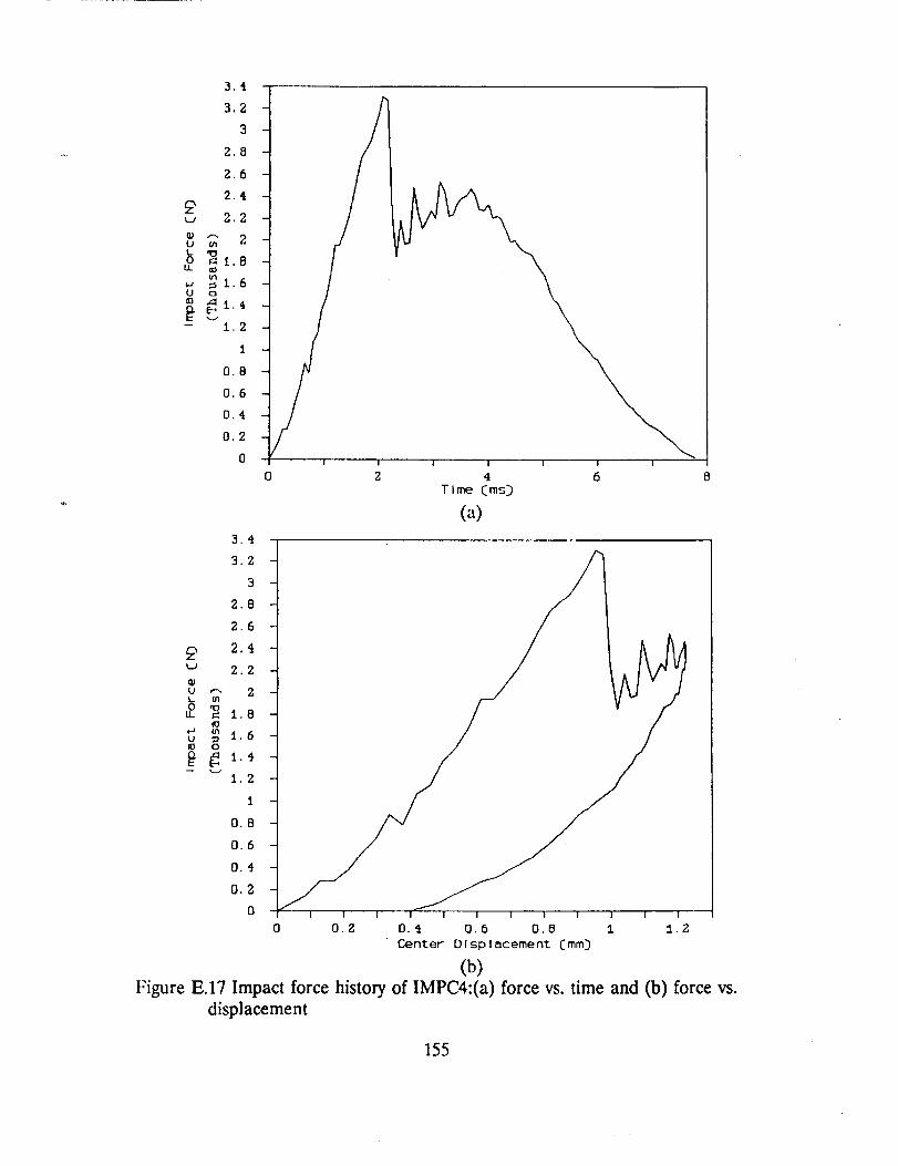
3.'L

3.2

3

2,8

2.6

2.4

_ 2.2

_ mt_

o _1,8U_ ¢0

U o

- 1.2

0.8

0.6

0.4

0.2

3.4

3.2

3

2..8

2.6

2.4_-_ 2.2

"-" 2

u _ 1.6e0 o

1.2

1

0.8

0.6

0.4

0.2

0

0.4 0.6 0.8

Center Olsplacement Cmrn:)

(b)Figure E.17 Impact force history of IMPC4:(a) force vs. time and (b) force vs.

displacement

155

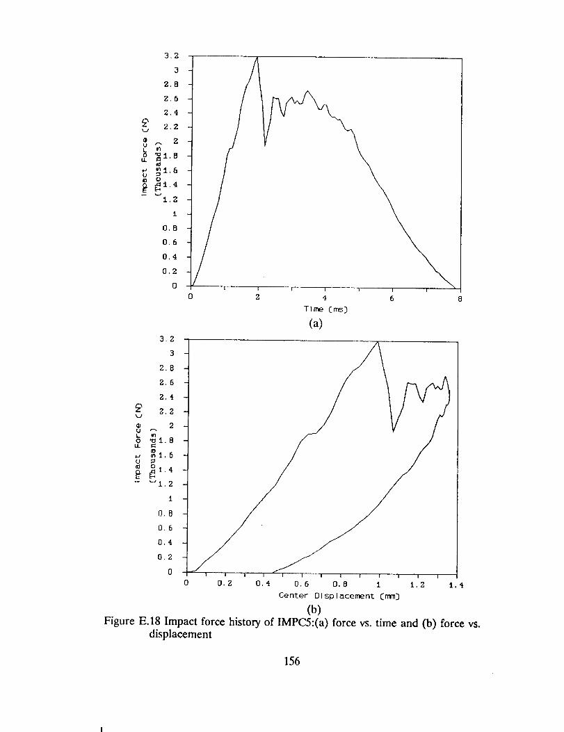
3.2

3

2.8

2.6

2.4

2.2

• 2U '--"

In

b _i.8U.

1,2

O.B

0.6

0.4

0.2

3.2

3

2.8

2.6

z.zkJ

2Uk

o _I.8

© _I.4

- ui. 2

0,8

0.6

0,4

0.2

I I

Time Cms3

(a)

0I

1,2

Figure E.18 Impact force history of IMPC5:(a) force vs. time and (b) force vs.displacement

156

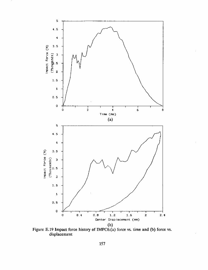
5

4.5

r_ 3.5Zk_J

u 2 3L

U 0

1..5

0.5

0

0I !

4

Time Cms)

(a)


157

£x.d

t o 0U

I !

2

I I

6

£

U_ 4U

U

0.4 0,8! I I I i

1.2 1.6 2

Center Displacement C_)

(b)

I I I I

2.4 2,8


158

REFERENCES

ASTM Designation: D 3039-76, "Standard Test Method for Tensile Properties

of Fiber-Resin Composites," ASTM Stondards and Literature References for

Composite M_terials, American Society for Testing and Materials,

Philadelphia, 1987, pp. 35-40.

Bostaph G. M., and Elber, W., "Static Indentation Tests on Composite Plates for

Impact Susceptibility Evaluation," Proceedings of the Army Symposium on

Solid Mechanics, AMMRC MS 82-4, U.S. Army, Sept. 1982, pp. 288-317.

Dost, E. F., licewicz, L. B., and Gosse, J. H., "Sublaminate Stability Based Modeling

of Impact-Damaged Composite Laminates," Proceedings of the American Society

for Composites 3rd Technical Conference, Seattle, Washington, September 1988,

pp. 354-363.

Ireland, D. R., "Procedures and Problems Associated with Reliable Control of the

Instrumented Impact Test," ASTM STP 563, 1974, pp. 3-29.

McConnell, V. P., "Composites after Defense: Where are the Opportunities?,"

Advanced Composites, Vol. 6, No.l, 1991, pp. 24-30.

Pinheiro, M. A. S., "Finite Elements for Free Edge Delaminations and Delaminated

Anisotropic Beams," Ph.D Dissertation, University of Florida, Gainesville,Florida, 1991

Sankar, B. V., "Contact Law for Transversely Isotropic Materials," Proceedings of

AIAA/ASME/ASCE/AHS 26th SDM conference, Orlando, Florida, 1985, pp.516-521.

Sankar, B. V., "Interlaminar Shear Stresses in Composite Laminates Due to Static

Indentation," J. Reinforced Plastics and Composites, Vol. 8, 1989, pp. 458-471.

Sankar, B. V., Ku, C., and Nguyen, P. T., "Nondimensional Impact Models for

Composite Laminates," Proceedings of the American Society for Composites 5th

Technical Conference, E. Lansing, Michigan, June 1990, pp. 600-610.

Sj6blom, P. O., Hartness, J. T., and Cordell, T. M., "On Low-Velocity Impact Testing

of Composite Materials," J. Composite Materials, Vol. 22, 1988, pp. 30-52.

Timoshenko, S., and Woinowsky-Krieger, S., Theory of Plates and Shells, McGraw-Hill, New York, 1959.

159

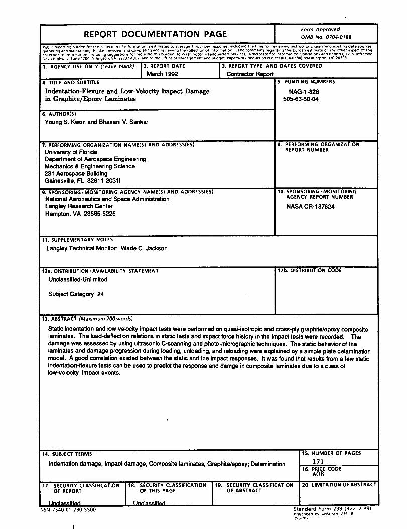
Form Approved

REPORT DOCUMENTATION PAGE OMBNo oTo4orea

Public reDortlng Dufden for this collecl:lon of informat*on bs estlrnatect to average I hour Der rescx3nse, includh"_g the time for reviewing Instructions, searching existing data sOurces,

gathering anti malnta#nlng the data neecled, ancl comoletlng ana rewewtncj the collectBon of _nformatlon Send commen_s rec_arding this burden estimate or any other asDect of th_scollection of information, JncIc_dlr_g suggestions for reducing thl_ Dur(_en tO Washtngton Headquarters Services. Directorate 1or Irlformatlon ODera_lons and ReDorts, 1215 Jefferson

Davis Highway, Suite 1204, ArimcJton, VA 22202-4302_ and to the Ofh_e of evlanagement and Budget, Paperwork Recluction Pro ect (0704-018R). Washington, OC 20S03

1. AGENCY USE ONLY (Leave blank) 2. REPORT DATE

March 1992

4. TITLE AND SUBTITLE

Indentstion-Flexure and Low-Velocity Impact Damagein Graphite/Epoxy Laminates

6. AUTHOR(S)

Young S. Kwon and Bhavani V. Sankar

7. PERFORMINGORGANIZATIONNAME(S) AND ADDRESS(ES)

University of FloridaDepartment of Aerospace EngineeringMechanics & Engineering Science231 Aerospace BuildingGainasville. FL 32611-20311

9. SPONSORING/MONITORINGAGENCYNAME(S) AND ADDRESS(ES)

National Aeronautics and Space AdministrationLangley Research CenterHampton, VA 23665-5225

3. REPORT TYPE AND DATES COVERED

Contractor Report!5, FUNDING NUMBERS

NAG-I-826505-63-50-O4

8. PERFORMING ORGANIZATIONREPORT NUMBER

10. SPONSORING / MONITORINGAGENCY REPORT NUMBER

NASA GR-187624

11. SUPPLEMENTARY NOTES

Langley Technical Monitor: Wade C. Jackson

12a. DISTRIBUTION/ AVAILABILITYSTATEMENT

Unclassified-Unlimited

Subject Category 24

12b. DISTRIBUTION CODE

13. ABSTRACT (Maximum 200words)

Static indentation and iow-velodty impact tests were performed on quasi-isotropic and cross-ply graphite/epoxy compositelaminates. The load-deflection relations in static tests and impact force history in the impact tests were recorded. Thedamage was assessed by using ultrasonic C-scanning and photo-micrographic techniques. The static behavior of thelaminates and damage progression during loading, unloading, and reloading were explained by a simple plate delaminationmodel. A good correlation existed between the static and the impact responses. It was found that results from a few staticindentation-flexure tests can be used to predict the response and damge in composite laminates due to a class ofIow-veiocity impact events.

14. SUBJECT TERMS

Indentation damage, Impact damage, Composite laminates, Graphite/epoxy; Delarnination

17. SECURITY CLASSIFICATION 18. SECURITY CLASSIFICATION 19.OF REPORT OF THIS PAGE

Unnlasmifiecl [JnPIn_=_=ifi=_l

NSN 7540-01-280-5S00

SECURITY CLASSIFICATION

OF ABSTRACT

15. NUMBER OF PAGES

17116. PRICE CODE

A08

20. LIMITATION OF ABSTRACT

Standard Form 298 (Rev 2-89)PrescrlD_N:l by ANSI StO Z39-18

298-102

Documents

NASA CONTRACTOR REPORT 187624 INDENTATION … · f / / =i • / nasa contractor report 187624 d indentation-flexure and low-velocity impact damage in graphite/epoxy laminates young