N-intertwined SIS epidemic network model · The N-intertwined SIS epidemic network model 149 two series for y∞ are given, whose coefﬁcients obey recursion relations, speciﬁed

Computing (2011) 93:147–169DOI 10.1007/s00607-011-0155-y

The N-intertwined SIS epidemic network model

Piet Van Mieghem

Received: 21 September 2011 / Accepted: 27 September 2011 / Published online: 13 October 2011© The Author(s) 2011. This article is published with open access at Springerlink.com

Abstract Serious epidemics, both in cyber space as well as in our real world, areexpected to occur with high probability, which justifies investigations in virus spreadmodels in (contact) networks. The N -intertwined virus spread model of the SIS-typeis introduced as a promising and analytically tractable model of which the steady-statebehavior is fairly completely determined. Compared to the exact SIS Markov model,the N -intertwined model makes only one approximation of a mean-field kind thatresults in upper bounding the exact model for finite network size N and improves inaccuracy with N . We review many properties theoretically, thereby showing, besidesthe flexibility to extend the model into an entire heterogeneous setting, that muchinsight can be gained that is hidden in the exact Markov model.

Keywords Epidemics · Networks · Robustness · Mean-field approximation

Mathematics Subject Classification (2000) 05C50 · 05C82 · 37H20 · 46N10 ·46N30 · 60J28

1 Introduction

We investigate the influence of the network topology on the spread of viruses, whosedynamics is modeled by a susceptible-infected-susceptible (SIS) type of process. TheSIS disease model [1,3,10] can be regarded as one of the simplest virus infectionmodels, in which persons or nodes in a network are either in two states: “healthy, butsusceptible to infection” or “infected by the disease or virus and, thus, infectious toneighbors”. In this article, the word “virus” is understood in the most general wordingpossible as an “item” transferred from the surroundings towards a node in the network.

P. Van Mieghem (B)Faculty of Electrical Engineering, Mathematics and Computer Science,Delft University of Technology, P.O. Box 5031, 2600 GA, Delft, The Netherlandse-mail: [email protected]

123

148 P. Van Mieghem

At a node, the “item” can be destroyed, but can also be propagated to neighbors ofthat node. For example, digital viruses (of all kind, and generally called malware)are living in cyberspace and use mainly the Internet as the transport media, whilebiological viruses contaminate other living beings and use “contacts” among theirvictims as their propagation network. A digital “virus” here can also mean a rumor,news or any kind of information that spreads over a data communications or socialnetwork. Recently, Hill et al. [17] have considered happiness of persons as a formof social infection and have modeled the spread of emotions over the social contactnetwork as a SIS-type of epidemic.

Our SIS, continuous-time model for the spreading of a virus in a network, called theN -intertwined virus spread model [36], is reviewed in Sect. 2. It was earlier consid-ered by Ganesh et al. [13] and by Wang et al. [40] in discrete-time, whose paper waslater improved in [7] after which their discrete-time model also appeared in the physicscommunity [15]. An infected node can infect its neighbors with an infection rate β (perlink), but it is cured with curing rate δ (per node). However, once cured and healthy, thenode is again prone to the virus. Both infection and curing processes are independent.There exists a wealth of variants or refinements of the SIS model (see e.g. [2,10,14,21,41]): there can be an incubation period, an infection rate that depends on the num-ber of neighbors or that has a constant component (as in [17]), a curing process thattakes a certain amount of time, and many other sophistications that we do not considerhere. Whereas most of the recent contributions to epidemics in networks were made byphysicists, Durrett [12] doubts about the mathematical rigor of many of their analyses.

A remarkable property of the SIS model is the appearance of a phase-transition[4,6] when the effective infection rate τ = β

δapproaches the epidemic threshold

τc = 1λ1

, where λ1 is the largest eigenvalue of the adjacency matrix A, also called thespectral radius. Below the epidemic threshold, τ < τc, the network is virus-free in thesteady-state, while for τ > τc, there is always a fraction of nodes that remains infected.For the companion infection model, SIR, where R stands for recovered or removed,Kermack and McKendrick [19] have shown that no epidemic can occur if the popu-lation density is below a critical threshold. Recently, Youssef and Scoglio [43] haveextended the N -intertwined SIS model to SIR epidemics and they have shown that theSIR-epidemic threshold also equals τc;SIR = 1

λ1. We point here to another dynamic

process on a network, that bears resemblance to virus spread. The synchronization ofcoupled oscillators in a network features a surprisingly similar phase transition: theonset of oscillator coupling occurs [28] at a critical coupling strength gc = g0

λ1and the

behavior of the phase transition around gc is mathematically similar [31]. Synchroni-zation [29] plays a role in sensor networks, human body (heart beat, brain, epilepsy),light emission of fire-flies, etc.

The major goal of this article is to provide a consistent, theoretical overview ofthe steady-state in the N -intertwined virus spread model, that we consider as almostcompletely solved since the recent solution [31] of the behavior around the epidemicthreshold. Section 2 explains the N -intertwined SIS virus spread model and the mean-field approximation. From Sect. 3 on, we confine to the steady-state of the N -inter-twined SIS model and present general equations for the fraction y∞ of steady-stateinfected nodes, from which the continued fraction expansion is derived. In addition,

123

The N -intertwined SIS epidemic network model 149

two series for y∞ are given, whose coefficients obey recursion relations, specifiedin Lemmas 1 and 3. Section 3.2 specifies the condition for the epidemic thresholdτc = 1

λ1and the behavior of y∞ (τ ) around τc, with references to many approaches

in networks to enlarge the epidemic threshold. After arguing that the transform s = 1τ

is more natural, bounds on y∞ (s) around s = 2E[D] are presented in Sect. 4 inspired

by simulations in [42] indicating that y∞ (s) is close to 12 for s = 2

E[D] . Section 5discusses the viral conductance ψ of a virus spreading process in a graph, that wasfirst proposed in [20]. We end our review by extending the N -intertwined model to aheterogeneous setting in Sect. 6: the governing equation and the continued fraction arereadily found, while the convexity Theorem 5 has interesting applications in networkprotection strategies [16,26]. Section 7 concludes with an outlook on open problems.

2 The N-intertwined SIS model

A network is represented by an undirected graph G (N , L) with N nodes and L links.The network topology is described by a symmetric adjacency matrix A, in which theelement ai j = a ji = 1 if there is a link between nodes i and j , otherwise ai j = 0. Inthe sequel, we confine ourselves and make the following simplifying assumptions. Thestate of a node i is specified by a Bernoulli random variable Xi ∈ {0, 1}: Xi = 0 for ahealthy node and Xi = 1 for an infected node. A node i at time t can be in one of the twostates: infected, with probability vi (t) = Pr[Xi (t) = 1] or healthy, with probability1−vi (t). We assume that the curing process per node i is a Poisson process with rate δ,and that the infection rate per link is a Poisson process with rateβ. All involved Poissonprocesses are independent. The effective infection rate is defined as τ = β

δ. We assume

that the initial infection state vi (0) in each node i is known. This is the general descrip-tion of the simplest type of a SIS virus spread model in a network and the challenge is todetermine the virus infection probability vi (t) for each node i in the graph G at time t .

This SIS model can be expressed exactly in terms of a continuous-time Markovmodel with 2N states as shown in [36]. Unfortunately, the exponentially increasingstate space with N prevents the determination of the set of {vi (t)}1≤i≤N in realisticnetworks, which has triggered a spur of research to find good approximate solutions.For an overview of SIS heuristics and numerous extensions, we refer to [4,21,42].

In contrast to all published SIS-type of models, the N -intertwined model, proposedand investigated in depth in [36], only makes one (mean-field) approximation in theexact SIS model and is applicable to all graphs.

2.1 The mean-field approximation

By separately observing each node, every node i at time t in the network has twostates: infected with probability vi (t) = Pr[Xi (t) = 1] and healthy with probabilityPr[Xi (t) = 0] = 1−vi (t). If we apply Markov theory straight away, the infinitesimalgenerator Qi (t) of this two-state continuous Markov chain is,

Qi (t) =[−q1;i q1;i

q2;i −q2;i

]

123

150 P. Van Mieghem

Fig. 1 The mean-field approximation (arrow) transforms the random variable q1; j into the averageE[q1; j

]. Instead of being infected at time t by the precise number of infected neighbors, the node i is

now infected by the average number of infected neighbors

with q2;i = δ is the curing rate and

q1;i = β

N∑j=1

ai j 1{X j (t)=1}

where the indicator function 1x = 1 if the event x is true else it is zero. The rate q1;iequals the sum over all infection rates of infected neighbors of node i and this rate q1;icouples or “intertwines” node i to the rest of the network through the appearance ofthe events

{X j (t) = 1

}. As mentioned in [36], the total infection rate q1;i is a random

variable, whereas ordinary Markov theory requires that q1; j is a real number. Therandom nature of q1;i is removed by an additional conditioning to all possible com-binations of rates, which is equivalent to conditioning to all possible combinations ofthe states X j (t) = 1 (and their complements X j (t) = 0) of the neighbors of node i .Hence, the number of basic states in the Markov process dramatically increases fromtwo states per node to all possible combinations of states for N nodes. Eventually,after conditioning each node in such a way, we end up with the exact 2N -state Markovchain, specified in [36].

Instead of conditioning, the mean-field approximation consists of replacing q1;i byits average E

[q1;i

], which is a real number and allows immediate application of con-

tinuous-time Markov theory [30]. Figure 1 illustrates the mean-field approximation.Using E [1x ] = Pr [x], we replace q1;i by

E[q1;i

] = β

N∑j=1

ai j Pr[X j (t) = 1] = β

N∑j=1

ai jv j (t)

which results in an effective infinitesimal generator,

Qi (t) =[−E

[q1;i

]E[q1;i

]δ −δ

]

Due to the dependence of E[q1;i

]on v j (t), the Markov differential equation [30,

(10.11) on p. 182] for state Xi (t) = 1 turns out to be non-linear,

123


dvi (t)

dt= β(1 − vi (t))

N∑j=1

ai jv j (t)− δvi (t) (1)

The governing differential equation (1) in the N -intertwined model for a node i hasthe following physical interpretation: the time-derivative of the infection probabilityof a node i consists of two competing processes: (1) while healthy with probability

(1 − vi (t)), all infected neighbors, an event with probabilityN∑

j=1ai jv j (t), try to infect

the node i with rate β and (2) while infected with probability vi (t), the node i is curedat rate δ. This rather intuitive explanation has been directly used in former modelssuch as the Kephart and White model [18] to derive the differential equation, therebyimplicitly making a mean-field approximation.

Defining the vector V (t) = [v1 (t) v2 (t) · · · vN (t)

]T , the matrix representationbased on (1) becomes

dV (t)

dt= (βA − δ I ) V (t)− βdiag (vi (t)) AV (t) (2)

where diag (vi (t)) is the diagonal matrix with elements v1 (t) , v2 (t) , . . . , vN (t). Wedefine the (average) fraction of infected nodes in the network at time t as

y (t) = 1

NE

⎡⎣ N∑

j=1

1{X j (t)=1}⎤⎦ = 1

N

N∑j=1

v j (t) (3)

In [25,36], we show that the mean-field approximation implies that (a) the N -inter-twined model upperbounds the exact probability vi (t) of infection, (b) the deviationsbetween the N -intertwined and the exact model are largest for intermediate valuesof τ around τc and (c) the random variables X j and Xi are implicitly assumed tobe independent. Since the latter basic assumption is increasingly good for large N ,we expect that the deductions from the N -intertwined model are asymptotically (forN → ∞) almost exact for real-world networks.

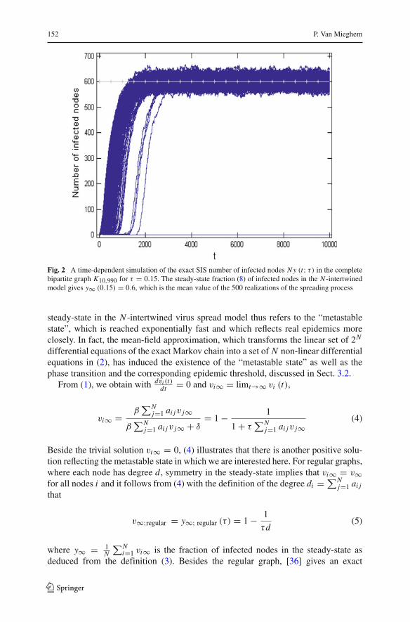
Figure 2 shows 500 sample paths of the exact SIS process, together with the steady-state fraction y∞ (τ ) of infected nodes. Although the steady-state fraction is constant,the SIS infection process continues for ever, which means that an arbitrary node imoves between the healthy and infected state for 1−vi∞ and vi∞ percent of the time,respectively.

3 The steady-state fraction y∞ of infected nodes

In this section, we focus on the steady-state of the N -intertwined model, wherevi∞ = limt→∞ vi (t) and limt→∞ dvi (t)

dt = 0. The corresponding steady-state vectoris denoted by V∞. In the exact SIS model, the steady-state is the healthy state, whichis the only absorbing state in the Markov process. However, in networks of realisticsize N , this steady-state is only reached after an unrealistically long time [13]. The

123

152 P. Van Mieghem

Fig. 2 A time-dependent simulation of the exact SIS number of infected nodes N y (t; τ) in the completebipartite graph K10,990 for τ = 0.15. The steady-state fraction (8) of infected nodes in the N -intertwinedmodel gives y∞ (0.15) = 0.6, which is the mean value of the 500 realizations of the spreading process

steady-state in the N -intertwined virus spread model thus refers to the “metastablestate”, which is reached exponentially fast and which reflects real epidemics moreclosely. In fact, the mean-field approximation, which transforms the linear set of 2N

differential equations of the exact Markov chain into a set of N non-linear differentialequations in (2), has induced the existence of the “metastable state” as well as thephase transition and the corresponding epidemic threshold, discussed in Sect. 3.2.

From (1), we obtain with dvi (t)dt = 0 and vi∞ = limt→∞ vi (t),

vi∞ = β∑N

j=1 ai jv j∞β∑N

j=1 ai jv j∞ + δ= 1 − 1

1 + τ∑N

j=1 ai jv j∞(4)

Beside the trivial solution vi∞ = 0, (4) illustrates that there is another positive solu-tion reflecting the metastable state in which we are interested here. For regular graphs,where each node has degree d, symmetry in the steady-state implies that vi∞ = v∞for all nodes i and it follows from (4) with the definition of the degree di = ∑N

j=1 ai j

that

v∞;regular = y∞; regular (τ ) = 1 − 1

τd(5)

where y∞ = 1N

∑Ni=1 vi∞ is the fraction of infected nodes in the steady-state as

deduced from the definition (3). Besides the regular graph, [36] gives an exact

123


solution of the steady-state infection behavior in the complete bipartite graph Km,n ,where there are two partitions Nm with m nodes and Nn with n nodes [32] so thatN = m + n and L = mn,

vi∞ = mn − 1τ 2( 1

τ+ m

)n

i ∈ Nn (6)

and

v j∞ = mn − 1τ 2( 1

τ+ n

)m

j ∈ Nm (7)

Thus, since y∞ = nvi∞+mv j∞n+m , we obtain

y∞ (τ ) =(mn − τ−2

)N

{1

τ−1 + m+ 1

τ−1 + n

}(8)

The complete bipartite graph, of which the star K1,n is a special case, often appearsas our benchmark model (see e.g. [22,23,33]).

The nodal infection steady-state equation (4) can be solved, as proved in [36] andalternatively in [33]:

Theorem 1 For any effective spreading rate τ = βδ

≥ 0, the non-zero steady-stateinfection probability of any node i in the N-intertwined model can be expressed as acontinued fraction

vi∞ = 1 − 1

1 + τdi − τ∑N

j=1ai j

1+τd j −τ∑Nk=1

a jk

1+τdk−τ∑Nq=1

akq

1+τdq −...

(9)

where di = ∑Nj=1 ai j is the degree of node i . Consequently, the exact steady-state

infection probability of any node i is bounded by

0 ≤ vi∞ ≤ 1 − 1

1 + τdi(10)

The interesting feature of the continued fraction (9) is that each convergent is anupper bound for vi∞. Another, equally useful, representation for vi∞ is the Laurentseries, proved in [33]:

Lemma 1 The Laurent series of the steady-state infection probability

vi∞ (τ ) = 1 +∞∑

m=1

ηm (i) τ−m (11)

123

154 P. Van Mieghem

possesses the coefficients

η1 (i) = − 1

di(12)

and

η2 (i) = 1

di

⎛⎝ 1

di+

N∑j=1

ai j

d j

⎞⎠ (13)

and for m ≥ 2, the coefficients obey the recursion

ηm+1 (i) = − 1

di

⎧⎨⎩ηm (i)

⎧⎨⎩1 −

N∑j=1

ai j

d j

⎫⎬⎭+

m∑k=2

ηm+1−k (i)N∑

j=1

ai jηk ( j)

⎫⎬⎭ (14)

Consequently, the Laurent series for the steady-state fraction of infected nodesequals

y∞ (τ ) = 1 + 1

N

∞∑m=1

{N∑

i=1

ηm (i)

}τ−m (15)

3.1 General relations for y∞

Summing (1) over all i is equivalent to right multiplication of V (t) by the all onevector uT because

∑Ni=1 vi (t) = uT V (t). Then, we find from (2) that

duT V (t)

dt= uT (diag (1 − vi (t)) βA − δ I ) V (t)

= β (u − V (t))T AV (t)− δuT V (t)

Hence, we obtain a relation for y∞ ∈ [0, 1] in terms of the vector V∞:

N y∞ = uT V∞ = τ (u − V∞)T AV∞ (16)

Since uT A = DT because A = AT , we can write (16) as

y∞ (τ ) = τ

N

(DT V∞ − V T∞ AV∞

)(17)

We write the degree vector D as D = �u, where � = diag(d1, d2, . . . , dN ), so that

N y∞ = τ(

uT�V∞ + V T∞�V∞ − V T∞�V∞ − V T∞ AV∞)

= τ((u − V∞)T �V∞ + V T∞ (�− A) V∞

)

123


Introducing the Laplacian Q = � − A of the graph G, the steady-state fraction ofinfected nodes y∞ is expressed as a quadratic form in terms of the Laplacian,

y∞ = τ

N

((u − V∞)T �V∞ + V T∞QV∞

)(18)

After left-multiplication of the steady state version of (2) by the vector

V T∞diag(vk−1

i∞)

= [vk

1∞ vk2∞ · · · vk

N∞]T

which we denote by(V k∞

)T, we obtain the scalar

(V k∞

)TV∞ =

N∑j=1

vk+1j∞ = τ

((V k∞

)TAV∞ −

(V k+1∞

)TAV∞

)(19)

For k = 0 in (19), and introducing the all one vector u = limk→0 V k∞, we obtain (16)again. For k = 1 in (19), the norm ‖V∞‖2

2 = V T∞V∞ = ∑Nj=1 v

2j∞ obeys

V T∞V∞ = τ(

V T∞ AV∞ − V T∞diag (vi∞) AV∞)

(20)

When summing (19) over all k from m ≥ 0 to infinity and taking∣∣v j∞

∣∣ < 1 intoaccount, the telescoping nature of the right-hand side leads to

∞∑k=m

(V k∞

)TV∞ =

N∑j=1

vm+1j∞

1 − v j∞= τ

(V m∞

)TAV∞ (21)

When m = 0, we have that V m∞ = u and we obtain, with the degree vector uT A = DT ,

1

τ

N∑j=1

v j∞1 − v j∞

= DT V∞ =N∑

j=1

d jv j∞ (22)

As shown earlier in [36], the characteristic structure (21) of the N -intertwined modelfollows more elegantly from the governing equation (2) in the steady-state

V∞ = τdiag (1 − vi∞) AV∞ (23)

for finite τ such that vi∞ < 1. Indeed, after left-multiplying both sides by(diag

(1 − vi∞

))−1 = diag( 1

1−vi∞), we have

1

τdiag

(1

1 − vi∞

)V∞ = AV∞

123

156 P. Van Mieghem

or

1

τ

V∞1 − V∞

= AV∞ (24)

where the vector(

V∞1−V∞

)T = [ v1∞1−v1∞

v2∞1−v2∞ · · · vN∞

1−vN∞]T

. By left-multiplication of

(24) by(V m∞

)T , we obtain (21) again.

3.2 Phase transition and epidemic threshold

Many authors (see e.g. [3,10,18,27]) mention the existence of an epidemic thresholdτc. If the effective spreading rate τ = β

δ> τc, the virus persists and a non-zero fraction

of the nodes are infected, whereas for τ ≤ τc, the epidemic dies out. The fact thatthe epidemic threshold occurs at τ = τc = 1

λ1has been proved in several papers, see

e.g. [7,36]. Here, we recall the fundamental lemma for the N -intertwined SIS model,proved in [36].

Lemma 2 There exists a value τc = 1λ1> 0 and for τ < τc, there is only the trivial

steady-state solution V∞ = 0. Beside the V∞ = 0 solution, there is a second, non-zerosolution for all τ > τc. For τ = τc + ε, it holds that V∞ = αx1, where ε, α > 0 arearbitrarily small constants and where x1 is the eigenvector belonging to the largesteigenvalue λ1 of the adjacency matrix A.

Lemma 2 has important practical consequences. Given a network with adjacencymatrix A and an imminent infection rate β, a nodal curing rate δ > βλ1 can be appliedin nodes (in the form of anti-virus software or any other protection scheme) to maintainthe network virus-free. A key-point is that the security of each host depends not onlyon the protection strategies it chooses to adopt but also on those chosen by other hostsin the network. In a heterogeneous setting, explained in Sect. 6, the resulting game-theoretic optimum has been studied in [26], while a different optimization techniquein [16] minimizes the overall infection in the network by determining the individualcuring rates of nodes. When the network can be modified, we possess a much largernumber of ways to ban epidemics such as immunization strategies [8] and severalways to decrease the spectral radius λ1 of the network: quarantining using the mod-ular form of the network [24], degree-preserving rewiring [34,38,39] that changesthe assortativity and modularity, and hence, the spectral radius. The optimal strategyto remove m links from the network in order to minimize λ1 is proved in [37] to beNP-hard. Consequently, several heuristics are proposed and evaluated in [37].

Lemma 2 shows that, for all graphs, V∞ = αx1 +ξ y, where y is a vector orthogonalto x1, α tends to zero as τ ↓ τc, while ξ tends faster to zero in that limit than α. Thefollowing theorem is proved in [31]:

Theorem 2 For any graph with spectral radius λ1 and corresponding eigenvector x1normalized such that xT

1 x1 = ∑Nj=1 (x1)

2j = 1, the steady-state fraction of infected

123


nodes y∞ obeys

y∞ (τ ) = 1

λ1 N

∑Nj=1 (x1) j∑Nj=1 (x1)

3j

(τ−1

c − τ−1)

+ O(τ−1

c − τ−1)2

(25)

when τ approaches the epidemic threshold τc from above.

Since the eigenvectors x1, x2, . . . , xN belonging to the eigenvalues λ1 ≥ λ2 ≥· · · ≥ λN of the adjacency matrix A span the N -dimensional vector space, we canwrite the steady-state infection probability vector V∞ (τ ) as a linear combination ofthe eigenvectors of A,

V∞ (τ ) =N∑

k=1

γk (τ ) xk (26)

where the coefficient γk (τ ) = xTk V∞ (τ ) is the scalar product of V∞ (τ ) and the eigen-

vector xk and where the eigenvector xk obeys the normalization xTk xk = 1. Physically,

(26) maps the dynamics V∞ (τ ) of the process onto the eigenstructure of the network,where γk (τ ) determines the importance of the process in a certain eigendirection ofthe graph. The definition y∞ (τ ) = 1

N uT V∞ (τ ) shows that

y∞ (τ ) = 1

N

N∑k=1

γk (τ ) uT xk (27)

Substitution of (26) into (16) yields

y∞ (τ ) = τ

N

N∑k=1

λkγk (τ )(

uT xk − γk (τ ))

(28)

For irregular graphs, generally, γm (τ ) = xTm V∞ (τ ) = 0 for m > 1 and all eigen-

values and eigenvectors in (28) play a role. Moreover, γm (τ ) can be negative, as wellas λm , while

∑Nk=1 λk = 0 (see [32, p. 30]). The larger the spectral gap λ1 − λ2 and

the smaller |λN |, the more y∞ is determined by the dominant k = 1 term in (28),and the more its viral behavior approaches that of a regular graph. Graphs with largespectral gap possess strong topological robustness [32], in the sense that it is difficultto tear that network apart.

Theorem 2 suggests, for all 1 ≤ k ≤ N , the existence of the power series

γk (τ ) =∞∑j=1

c j (k)(τ−1

c − τ−1) j

(29)

123

158 P. Van Mieghem

where c1 (k) = 0 for 2 ≤ k ≤ N , c1 (1) =(λ1∑N

j=1 (x1)3j

)−1and all other coeffi-

cients c j (k) can be determined in a recursive way as specified in the following lemma,which is proved in [33]:

Lemma 3 Defining

X (m, l, k) =N∑

q=1

(xm)q (xl)q (xk)q

the coefficients c j (m) in (29) obey, for m > 1 and j > 2, the recursion

c j (m) = c j−1 (m)

λ1 − λm{1 − c1 (1) (λ1 + λm) X (m,m, 1)}

− c1 (1)

λ1 − λm

N∑k=1;k =m

(λ1 + λk) c j−1 (k) X (m, k, 1)

− 1

λ1 − λm

j−2∑n=2

N∑l=1

N∑k=1

c j−n (l) cn (k) λk X (m, l, k)

while, for j = 2 and m > 1,

c2 (m) = − 1

λ1 − λm

X (m, 1, 1)

λ1 X2 (1, 1, 1)

and c1 (m) = 0. For m = 1, there holds that c1 (1) =(λ1∑N

j=1 (x1)3j

)−1and for

j > 1, the coefficients c j (1) satisfy the recursion

c j (1) = − 1

λ1 X (1, 1, 1)

N∑k=2

(λ1 + λk) c j (k) X (1, 1, k)

−j−1∑n=2

N∑l=1

N∑k=1

c j+1−n (l) cn (k) λk X (1, l, k)

The radius of convergence of the Laurent series (11) and of the series (29) is, ingeneral, unknown and still an open problem. From the definition (27), we obtain theseries expansion of y∞ (τ ) around τ−1

c − τ−1 as

y∞ (τ ) =∞∑j=1

{1

N

N∑k=1

c j (k) uT xk

}(τ−1

c − τ−1) j

(30)

123


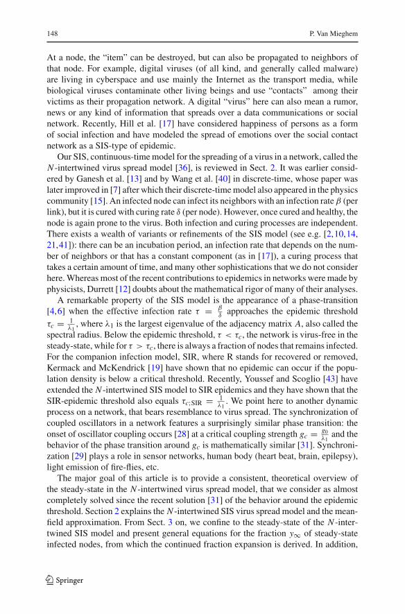
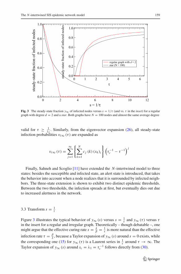
Fig. 3 The steady-state fraction y∞ of infected nodes versus s = 1/τ (and vs. τ in the inset) for a regulargraph with degree d = 2 and a star. Both graphs have N = 100 nodes and almost the same average degree

valid for τ ≥ 1λ1

. Similarly, from the eigenvector expansion (26), all steady-stateinfection probabilities vi∞ (τ ) are expanded as

vi∞ (τ ) =∞∑j=1

{N∑

k=1

c j (k) (xk)i

}(τ−1

c − τ−1) j

Finally, Sahneh and Scoglio [11] have extended the N -intertwined model to threestates: besides the susceptible and infected state, an alert state is introduced, that takesthe behavior into account when a node realizes that it is surrounded by infected neigh-bors. The three-state extension is shown to exhibit two distinct epidemic thresholds.Between the two thresholds, the infection spreads at first, but eventually dies out dueto increased alertness in the network.

3.3 Transform s = 1τ

Figure 3 illustrates the typical behavior of y∞ (s) versus s = 1τ

and y∞ (τ ) versus τin the insert for a regular and irregular graph. Theoretically – though debatable –, onemight argue that the effective curing rate s = δ

β= 1

τis more natural than the effective

infection rate τ = βδ

, because a Taylor expansion of y∞ (s) around s = 0 exists, whilethe corresponding one (15) for y∞ (τ ) is a Laurent series in 1

τaround τ → ∞. The

Taylor expansion of y∞ (s) around sc = λ1 = τ−1c follows directly from (30).

123

160 P. Van Mieghem

4 Behavior of y∞ (s) around s = E[D]2

In [25], we have shown, for any graph, that y∞ ≤ 12 for τ ≤ 1

E[D] . Moreover, sim-ulations in [25] indicate that the maximum variance for the N -intertwined model isreached for τ ≈ 2

E[D] .

Via extensive simulations, Youssef et al. [42] have observed that y∞ � 12 around

s = E[D]2 . In this section, several lemmas, proved in [33], explain and support these

simulations.

Lemma 4 For any graph, it holds that

y∞ (s) ≤ 1

2+ 1

2

(1 − E [D]

λ1

)for s = E [D]

2(31)

and equality is only possible for the regular graph.


y∞ (τ ) ≤ τ

(E [D]

4+ V T∞QV∞

N

)(32)

and equality is only possible for the regular graph for which V T∞QV∞ = 0.

Lemma 5 shows for the regular graph that the “tangent” line through the origin(τ = 0) lies above y∞; regular and only touches y∞; regular at the point τ = 2

E[D] = 2d .

For any other graph, the slope is not larger than E[D]4 + V T∞ QV∞

N and, after transformings = 1

τin (32), we find

y∞ (s) ≤ 1

2+ 2V T∞QV∞

N E [D]for s = E [D]

2(33)

that complements (31). The correction 12

(1− E[D]

λ1

)in (31) and the correction 2V T∞ QV∞

N E[D]

in (33) are positive and small, but nevertheless show that y∞ (s) can be larger than 12

at s = E[D]2 , as numerically found in [42].


y∞ (τ )

τ≥ r (τ ) = 1

N

N∑j=1

v j∞(d j − λ1v j∞

)(34)

where the lower bound obeys, for any τ ,

r (τ ) ≤ N2

4Nλ1

and where Nk = uT Aku denotes the number of walks of length k.

123


We will now estimate the value ξ for which r (ξ) = N24Nλ1

in irregular graphs where

Var[D] > 0. Provided that there exists a value of τ = ξ for which v j∞ (ξ) = d j2λ1

foreach 1 ≤ j ≤ N , that maximizes r (τ ), we have that

y∞ (ξ) = 1

N

N∑j=1

d j

2λ1= 1

2λ1

2L

N= 1

2

E [D]

λ1<

1

2

Lemma 6 then states that y∞ (ξ) ≥ ξN24Nλ1

or

1

λ1

L

N≥ ξN2

4Nλ1

from which

ξ ≤ 4L

N2= 2

E [D]

(E [D])2 + Var [D]<

2

E [D]

In conclusion, there may exist a value ξ such that τc < ξ < 2E[D] for which y∞ (ξ) =

12

E[D]λ1

< 12 .

We end by deducing, approximately though, another type of lower bound. Con-cavity of y∞ (τ ) for τ ≥ τc = 1

λ1similarly leads to y∞ (qτc + (1 − q)mτc) ≥

(1 − q) y∞ (mτc). For sufficiently large m, the Laurent series (11) up to first orderleads to

y∞ (mτc) ≥ 1 − 1

mτc N

N∑j=1

1

d j

because the second order term of O(

1(mτc)

2

)is positive due to η2 (i) > 0 in (13).

Choosing qτc + (1 − q)mτc = 2E[D] provides us with

y∞(

2

E [D]

)≥

2E[D] − τc

(m − 1) τc

⎛⎝1 − 1

mτc N

N∑j=1

1

d j

⎞⎠

>

(2λ1

E [D]− 1

)1

m

(1 − λ1 E

[ 1D

]m

)

Ignoring the integer nature of m, the maximizer of the right-hand side occurs atm = 2λ1 E

[ 1D

], resulting in

123

162 P. Van Mieghem

y∞(

2

E [D]

)�

2λ1E[D] − 1

4λ1 E[ 1

D

]

Notice that2λ1E[D] −1

4λ1 E[

1D

] ≤2λ1

E[D] −1

4 λ1E[D]

< 12 .

In summary, both last lower bound arguments illustrate, together with the upperbounds in Lemmas 4 and 5 that, for values of τ approaching 2

E[D] , the steady-state frac-

tion of infected nodes y∞ (τ ) is close to 12 in any graph, in agreement with simulations

[42].

5 The viral conductance

The viral conductance ψ of a virus spreading process in a graph was first proposedin [20] as a new graph metric and then elaborated in more detail in [42]. The viralconductance ψ is defined as

ψ =λ1∫

0

y∞ (s) ds (35)

where s = 1τ

and λ1 is the spectral radius (i.e. the largest eigenvalue of the adja-cency matrix A of the graph) and equal to sc = 1

τc. Below the epidemic threshold

τc, the network is virus-free in the steady-state. Hence, vi∞ (τ ) = 0 for τ < τc, andequivalently, vi∞ (s) = 0 for s > 1

τc= λ1. Since the function y∞ (τ ) versus τ is not

integrable over all τ , Kooij et al. [20] have proposed to consider y∞( 1τ

)versus s = 1

τ(see Fig. 3).

In most published work so far, network G1 was considered to be more robustagainst virus spread than network G2 if the epidemic threshold τc (G1) > τc (G2).For example, in Fig. 3, the regular graph with the same number N of nodes and nearlythe same number L of links possesses a higher epidemic threshold than the star, and,thus, according to the above robustness criterion, the regular graph is more robustagainst virus propagation than the star. However, when the effective infection rateτ > 1 = 2τc

(Gregular

), we observe from Fig. 3 that the percentage of infected nodes

in the star is smaller than in the regular graph. The extent of the virus-free region is oneaspect of the network’s resilience against viruses, but once that barrier, the epidemicthreshold, is crossed, the virus may conduct differently in networks with high andlow epidemic threshold. This observation has led Kooij et al. [20] to propose the viralconductance as an additional metric.

The viral conductance ψ is a graph metric that represents the overall conductanceof the virus for all possible effective infection rates τ : when ψ is high for the graphG, the virus can spread easily in G. Thus, instead of grading graphs only based ontheir epidemic threshold τc from virus vulnerable, where τc is small (high spectralradius λ1) to virus robust (where τc is large), the viral conductance complements thisclassification with an average infection notion because

123


y∞ = 1

λ1

λ1∫0

y∞ (s) ds < 1

so that ψ = y∞τc< 1

τc= λ1. Graphs with small epidemic threshold may possess a

small average fraction of infected nodes y∞ so that the viral conductance can be equalto graphs with large epidemic threshold and large y∞.

Using both expansions (15) and (30) into the definition (35) of ψ yields, subject tothe condition that the radius of convergence of both series is at least λ1

2 ,

ψ = λ1

2− 1

N

{N∑

k=1

1

dk− uT x1

λ1∑N

j=1 (x1)3j

}λ2

1

8+ R

where the remainder is

R = 1

N

∞∑m= j

{N∑

k=1

ηm (k)+ cm (k) uT xk

}(λ1)

m+1

2m+1 (m + 1)

Subject to the above convergence condition, the expansion R j can be numerically com-puted up to any desired accuracy when the adjacency matrix A is given, from whichthe eigenvectors x1, x2, . . . , xN belonging to the eigenvalues λ1 ≥ λ2 ≥ · · · ≥ λN

can be computed.Several bounds for the viral conductance are derived in [33] of which we only

recall here a few. A simple upper bound, deduced from the convexity of y∞ (s) ins ∈ [0, λ1), is

ψ ≤ λ1

2

More accurate lower and upper bounds are

ψ ≥ λ1

2

{Z + ζ (1 − Z)+ mins∈[0,λ1] y′′∞ (s)

3

{λ2

1 − 3λ1ζ + 3ζ 2}}

(36)

and

ψ ≤ λ1

2

{Z + ζ (1 − Z)+ maxs∈[0,λ1] y′′∞ (s)

3

{λ2

1 − 3λ1ζ + 3ζ 2}}

where Z = 1N

∑Nj=1(x1) j∑Nj=1(x1)

3j< 1 and ζ = 1−Z

λ1 E[

1D

]−Z

≤ 1. Other types of bounds are

dmin

2≤ ψ < ln

(1 + λ1

dmin − 1

){E [D] − 1}

123

164 P. Van Mieghem

The largest possible ratio λ1dmin

= O(√

N)

occurs in the star, which illustrates that the

viral conductance is bounded by 12 E [D] log N . Likely, the star possesses the largest

viral conductance among all graphs with N nodes and L links. It is further conjecturedin [42] that the regular graph attains the lowest viral conductance all graphs with Nnodes and L links. This conjecture has only partially been proved so far in [33] to betrue for the class of complete bipartite graphs, but not yet for all graphs.

6 Heterogeneous N-intertwined model

The homogenous N -intertwined model, where the infection and curing rate is the samefor each link and node in the network, has been extended to a heterogeneous settingin [35], where an infected node i can infect its neighbors with an infection rate βi , butit is cured with curing rate δi .

Heterogeneity rather than homogeneity abounds in real networks. For example, indata communications networks, the transmission capacity, age, performance, installedsoftware, security level and other properties of networked computers are generally dif-ferent. Social and biological networks are very diverse: a population often consistsof a mix of weak and strong, or old and young species or of completely differenttypes of species. The network topologies for transport by airplane, car, train, ship aredifferent. Many more examples can be added illustrating that homogeneous networksare the exception rather than the rule. This diversity in the “nodes” and “links” of realnetworks will thus likely affect the spreading pattern of viruses. In previous Sections,only a homogeneous virus spread was investigated, where all infection rates βi = β

and all curing rates δi = δ were the same for each node. We believe that the extensionto a full heterogeneous setting is, perhaps, the best SIS model that we can achieve.

The governing differential equation (1) is straightforwardly generalized to

dvi (t)

dt=

N∑j=1

β j ai jv j (t)− vi (t)

⎛⎝ N∑

j=1

β j ai jv j (t)+ δi

⎞⎠ (37)

while the corresponding matrix equation is

dV (t)

dt= Adiag

(β j)

V (t)− diag (vi (t))(

Adiag(β j)

V (t)+ C)

(38)

where diag(vi (t)) is the diagonal matrix with elements v1 (t) , v2 (t) , . . . , vN (t) andthe curing rate vector is C = (δ1, δ2, . . . , δN ). We note that A diag(βi ) is, in gen-eral and opposed to the homogeneous setting, not symmetric anymore, unless A anddiag(βi ) commute, in which case the eigenvalue λi (Adiag (βi )) = λi (A) βi and bothβi and λi (A) have a same eigenvector xi .

123


6.1 The steady-state

The metastable steady-state follows from (38) as

Adiag (βi ) V∞ − diag (vi∞) (Adiag (βi ) V∞ + C) = 0

where V∞ = limt→∞ V (t). We define the vector

w = Adiag (βi ) V∞ + C (39)

and write the stead-state equation as

w − C = diag (vi∞) w

or

(I − diag (vi∞)) w = C

Ignoring extreme virus spread conditions (the absence of curing (δi = 0) and an infi-nitely strong infection rate βi → ∞), then the infection probabilities vi∞ cannot beone such that the matrix (I − diag (vi∞)) = diag(1 − vi∞) is invertible. Hence,

w = diag

(1

1 − vi∞

)C

Invoking the definition (39) of w, we obtain

Adiag (βi ) V∞ = diag

(vi∞

1 − vi∞

)C

= diag

(δi

1 − vi∞

)V∞ (40)

that generalizes (24). The i-th row of (40) yields the nodal steady state equation,

N∑j=1

ai jβ jv j∞ = vi∞δi

1 − vi∞(41)

Let V∞ = diag(βi ) V∞ and the effective spreading rate for node i, τi = βiδi

, then wearrive at

Q(

1

τi (1 − vi∞)

)V∞ = 0 (42)

123

166 P. Van Mieghem

where the symmetric matrix

Q (qi ) = diag (qi )− A (43)

= diag (qi − di )+ Q

can be interpreted as a generalized Laplacian1, because Q (di ) = Q = �− A, where� = diag(di ). The observation that the non-linear set of steady-state equations can bewritten in terms of the generalized Laplacian Q (qi ) is fortunate, because the power-ful theory of the “normal” Laplacian Q applies. Many properties of the generalizedLaplacian Q (qi ) are given in [35] that enabled to prove three important theorems.The first theorem is

Theorem 3 The critical threshold is determined by vectors τc = (τ1c, τ2c, . . . , τNc)

that obey λmax (R) = 1, where λmax (R) is the largest eigenvalue of the symmetricmatrix

R = diag(√τi)

Adiag(√τi)

(44)

whose corresponding eigenvector has positive components if the graph G is connected.

Several bounds for λmax (R) are derived and λmax (R) for the complete graph KN

is solved exactly. The generalization of Theorem 1 is

Theorem 4 The non-zero steady-state infection probability of any node i in theN-intertwined model can be expressed as a continued fraction

vi∞ = 1 − 1

1 + γiδi

− δ−1i

∑Nj=1

β j ai j

1+ γ jδ j

−δ−1j

∑Nk=1

βk a jk

1+ γkδk

−δ−1k

∑Nq=1

aqkβq

...

(45)

where the total infection rate of node i , incurred by all neighbors towards node i , is

γi =N∑

j=1

ai jβ j =∑

j∈ neighbor(i)

β j (46)

Consequently, the exact steady-state infection probability of any node i is bounded by

0 ≤ vi∞ ≤ 1 − 1

1 + γiδi

Perhaps the most important theorem proved in [35] is

1 All eigenvalues of the Laplacian Q = � − A in a connected graph are positive, except for the smallestone that is zero. Hence, Q is positive semi-definite. Much more properties of the Laplacian Q are founde.g. in [5,9,32].

123


Theorem 5 Given that all curing rates δ j for 1 ≤ j = i ≤ N are constant andindependent from the infection rates β j , the non-zero steady-state infection proba-bility vi∞ (δ1, . . . , δi , . . . , δN ) > 0 is strict convex in δi , while all other non-zerosteady-state infection probabilities v j∞ (δ1, . . . , δi , . . . , δN ) > 0 are concave in δi .

A direct consequence of Theorem 5 to the homogeneous setting is that y∞ (s) isconvex for s ∈ [0, λ1) (or y∞ (τ ) is concave for τ > τc).

7 Conclusion

The N -intertwined SIS network model has been introduced and many derived resultsin the steady-state have been reviewed. While extensions of the model are certainlyexpected in the future, we believe that the steady-state theory of the homogeneousN -intertwined SIS network model is almost entirely established. The time-dependenttheory, on the other hand, needs much more efforts towards maturity. Although theN -intertwined model is not exact, the only—a mean-field—approximation has enabledanalytic computations as presented here that are, to the best of our knowledge, notpossible with any other SIS model that is more accurate than the N -intertwined model.An open problem is to determine of the overall accuracy of the N -intertwined model(with respect to the exact SIS Markov process) for any value of τ in a broad class ofinteresting networks. So far, numerical simulations [21] point to a promisingly goodaccuracy that improves with N .

A newly envisioned direction is the coupling of the virus spread process with theunderlying topology. In other words, the presented model has assumed that the adja-cency matrix A is fixed and is not changed by the virus spread process. Hence, nodescan only protect themselves against the virus by increasing their curing rate δ. Whiletaking medicine or vaccination is one measure in the fight against the virus, a morenatural one is to avoid contact with infected people. The latter assumes that the adja-cency matrix A is changed by the process and the knowledge that a node’s neighbor(s)is (are) infected. The precise description of the coupling between virus spread pro-cess and topology as well as the solution of the far more complex set of differentialequations stand on the agenda of future research.

Acknowledgements We are very grateful to Caterina Scoglio, Mina Youssef, Faryad Darabi Sahneh,Cong Li and Rob Kooij for many comments on an early version of the manuscript. This research wassupported by Next Generation Infrastructures (Bsik) and the EU FP7 project ResumeNet (project No.224619).

Open Access This article is distributed under the terms of the Creative Commons Attribution Noncom-mercial License which permits any noncommercial use, distribution, and reproduction in any medium,provided the original author(s) and source are credited.

References

1. Anderson RM, May RM (1991) Infectious diseases of humans: dynamics and control. Oxford Univer-sity Press, Oxford

2. Asavathiratham C (2000) The influence model: a tractable representation for the dynamics of networkedmarkov chains. Ph.D thesis, Massachusetts Institute of Technology, Cambridge

123

168 P. Van Mieghem

3. Bailey NTJ (1975) The mathematical theory of infectious diseases and its applications, 2nd edn. Char-lin Griffin & Company, London

4. Barrat A, Bartelemy M, Vespignani A (2008) Dynamical processes on complex networks. CambridgeUniversity Press, Cambridge

5. Biggs N (1996) Algebraic graph theory, 2nd edn. Cambridge University Press, Cambridge6. Castellano C, Pastor-Satorras R (2010) Thresholds for epidemic spreading in networks. Phys Rev Lett

105:2187017. Chakrabarti D, Wang Y, Wang C, Leskovec J, Faloutsos C (2008) Epidemic thresholds in real networks.

ACM Trans Inf Syst Secur (TISSEC) 10(4):1–268. Chen Y, Paul G, Havlin S, Liljeros F, Stanley HE (2008) Finding a better immunization strategy. Phys

Rev Lett 101:0587019. Cvetkovic DM, Doob M, Sachs H (1995) Spectra of fraphs, theory and applications, 3rd edn. Johann

Ambrosius Barth Verlag, Heidelberg10. Daley DJ, Gani J (1999) Epidemic modelling: an introduction. Cambridge University Press, Cambridge11. Darabi Sahneh F, Scoglio C (2011) Epidemic spread in human networks. In: 50th IEEE conference on

decision and control, Orlando, December 2011. arXiv:1107.2464v112. Durrett R (2010) Some features of the spread of epidemics and information on a random graph. Proc

Natl Acad Sci USA (PNAS) 107(10):4491–449813. Ganesh A, Massoulié L, Towsley D (2005) The effect of network topology on the spread of epidemics.

In: IEEE INFOCOM05, San Francisco14. Garetto M, Gong W, Towsley D (2003) Modeling malware spreading dynamics. In: IEEE INFO-

COM’03, San Francisco, April 200315. Gómez S, Arenas A, Borge-Holthoefer J, Meloni S, Moreno Y (2010) Discrete-time Markov chain

approach to contact-based disease spreading in complex networks. Europhys Lett (EPL) 89:3800916. Gourdin E, Omic J, Van Mieghem P (2011) Optimization of network protection against virus spread.

In: 8th international workshop on design of reliable communication networks (DRCN 2011), Krakow,10–12 October 2011

17. Hill AL, Rand DG, Nowak MA, Christakis NA (2010) Emotions as infectious diseases in a large socialnetwork: the SISa model. Proc Royal Soc B 277:3827–3835

18. Kephart JO, White SR (1991) Direct-graph epidemiological models of computer viruses. In: Proceed-ings of the 1991 IEEE computer society symposium on research in security and privacy, pp 343–359,May 1991

19. Kermack WO, McKendrick AG (1927) A contribution to the mathematical theory of epidemics. ProcRoyal Soc A 115:700–721

20. Kooij RE, Schumm P, Scoglio C, Youssef M (2009) A new metric for robustness with respect to virusspread. In: Networking 2009, LNCS 5550, pp 562–572

21. Omic J (2010) Epidemics in networks: modeling, optimization and security games. Ph.D thesis, Sep-tember 2010. http://repository.tudelft.nl/. Accessed Sept 2010

22. Omic J, Kooij RE, Van Mieghem P (2007) Virus spread in complete bi-partite graphs. In: Bionetics2007, Budapest, 10–13 December 2007

23. Omic J, Kooij RE, Van Mieghem P (2009) Heterogeneous protection in regular and complete bi-partitenetworks. In: IFIP networking 2009, Aachen, 11–15 May 2009

24. Omic J, Martin Hernandez J, Van Mieghem P (2010) Network protection against worms and cascadingfailures using modularity partitioning. In: 22nd international teletraffic congress (ITC 22), Amsterdam,7–9 September 2010

25. Omic J, Van Mieghem P (2009) Epidemic spreading in networks—variance of the number of infectednodes. Delft University of Technology, report20090707. http://www.nas.ewi.tudelft.nl/people/Piet/TUDelftReports

26. Omic J, Van Mieghem P, Orda A (2009) Game theory and computer viruses. In: IEEE Infocom0927. Pastor-Satorras R, Vespignani A (2001) Epidemic spreading in scale-free networks. Phys Rev Lett

86(14):3200–320328. Restrepo JG, Ott E, Hunt Brian R (2005) Onset of synchronization in large networks of coupled oscil-

lators. Phys Rev E 71(036151):1–1229. Strogatz SH (2000) From Kuramoto to Crawford: exploring the onset of synchronization in populations

of coupled oscillators. Physica D 143:1–2030. Van Mieghem P (2006) Performance analysis of communications systems and networks. Cambridge

University Press, Cambridge

123

http://repository.tudelft.nl/

http://www.nas.ewi.tudelft.nl/people/Piet/TUDelftReports



31. Van Mieghem P (2011) Epidemic phase transition of the SIS-type in networks (submitted)32. Van Mieghem P (2011) Graph spectra for complex networks. Cambridge University Press, Cambridge33. Van Mieghem P (2011) Viral conductance of a network (submitted)34. Van Mieghem P, Ge G, Schumm P, Trajanovski S, Wang H (2010) Spectral graph analysis of modu-

larity and assortativity. Phys Rev E 82:05611335. Van Mieghem P, Omic J (2008) In-homogeneous virus spread in networks. Delft University of Tech-

nology, Report2008081. http://www.nas.ewi.tudelft.nl/people/Piet/TUDelftReports36. Van Mieghem P, Omic J, Kooij RE (2009) Virus spread in networks. IEEE/ACM Trans Netw 17(1):

1–1437. Van Mieghem P, Stevanovic D, Kuipers FA, Li C, van de Bovenkamp R, Liu D, Wang H (2011) Decreas-

ing the spectral radius of a graph by link removals. Phys Rev E 84(1):01610138. Van Mieghem P, Wang H, Ge X, Tang S, Kuipers FA (2010) Influence of assortativity and degree-pre-

serving rewiring on the spectra of networks. E Phys J B 76(4):643–65239. Wang H, Winterbach W, Van Mieghem P (2011) Assortativity of complementary graphs. Eur Phys

J B (to appear)40. Wang Y, Chakrabarti D, Wang C, Faloutsos C (2003) Epidemic spreading in real networks: an eigen-

value viewpoint. In: 22nd international symposium on reliable distributed systems (SRDS’03), IEEEcomputer, pp 25–34, October 2003

41. Wang Y, Wang C (2003) Modeling the effects of timing parameters on virus propagation. In: ACMworkshop on rapid malcode (WORM’03), Washington DC, pp 61–66, 27 Oct 2003

42. Youssef M, Kooij RE, Scoglio C (2011) Viral conductance: quantifying the robustness of networkswith respect to spread of epidemics. J Comput Science. doi:10.1016/j.jocs.2011.03.001

43. Youssef M, Scoglio C (2011) An individual-based approach to SIR epidemics in contact networks.J Theor Biol 283:136–144

123


http://dx.doi.org/10.1016/j.jocs.2011.03.001

Documents

N-intertwined SIS epidemic network model · The N-intertwined SIS epidemic network model 149 two series for y∞ are given, whose coefﬁcients obey recursion relations, speciﬁed