Embed Size (px)
Citation preview
Chapter 14
Mysterious, Inconvenient, or WrongResults from Real Datasets
This chapter describes five examples in which my colleagues and I got mysterious,inconvenient, or plainly wrong results using mixed linear models to analyze realdatasets. All these examples involve the data’s information about f , the unknownsin the mixed linear model’s R or G, and thus lead to examination of the restrictedlikelihood and its close relative, the marginal posterior of f .
14.1 Periodontal Data and the ICAR Model
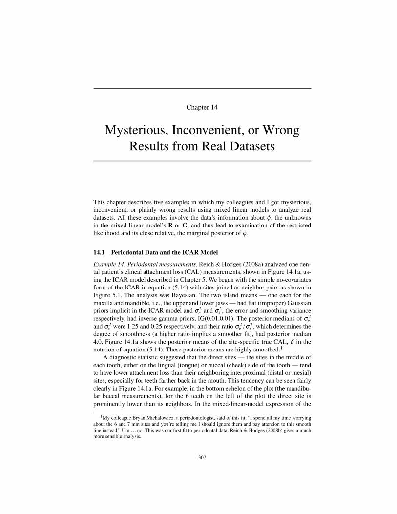
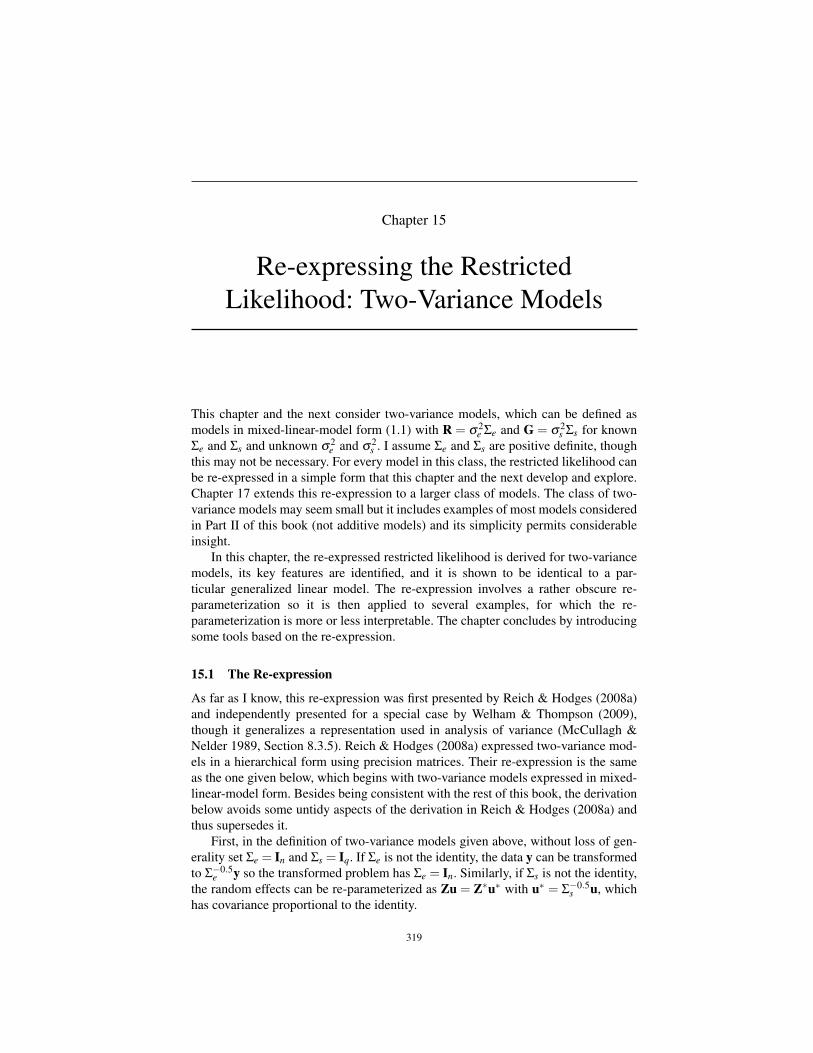
Example 14: Periodontal measurements. Reich & Hodges (2008a) analyzed one den-tal patient’s clincal attachment loss (CAL) measurements, shown in Figure 14.1a, us-ing the ICAR model described in Chapter 5. We began with the simple no-covariatesform of the ICAR in equation (5.14) with sites joined as neighbor pairs as shown inFigure 5.1. The analysis was Bayesian. The two island means — one each for themaxilla and mandible, i.e., the upper and lower jaws — had flat (improper) Gaussianpriors implicit in the ICAR model and s
2e and s
2s , the error and smoothing variance
respectively, had inverse gamma priors, IG(0.01,0.01). The posterior medians of s
2e
and s
2s were 1.25 and 0.25 respectively, and their ratio s
2e /s
2s , which determines the
degree of smoothness (a higher ratio implies a smoother fit), had posterior median4.0. Figure 14.1a shows the posterior means of the site-specific true CAL, d in thenotation of equation (5.14). These posterior means are highly smoothed.1
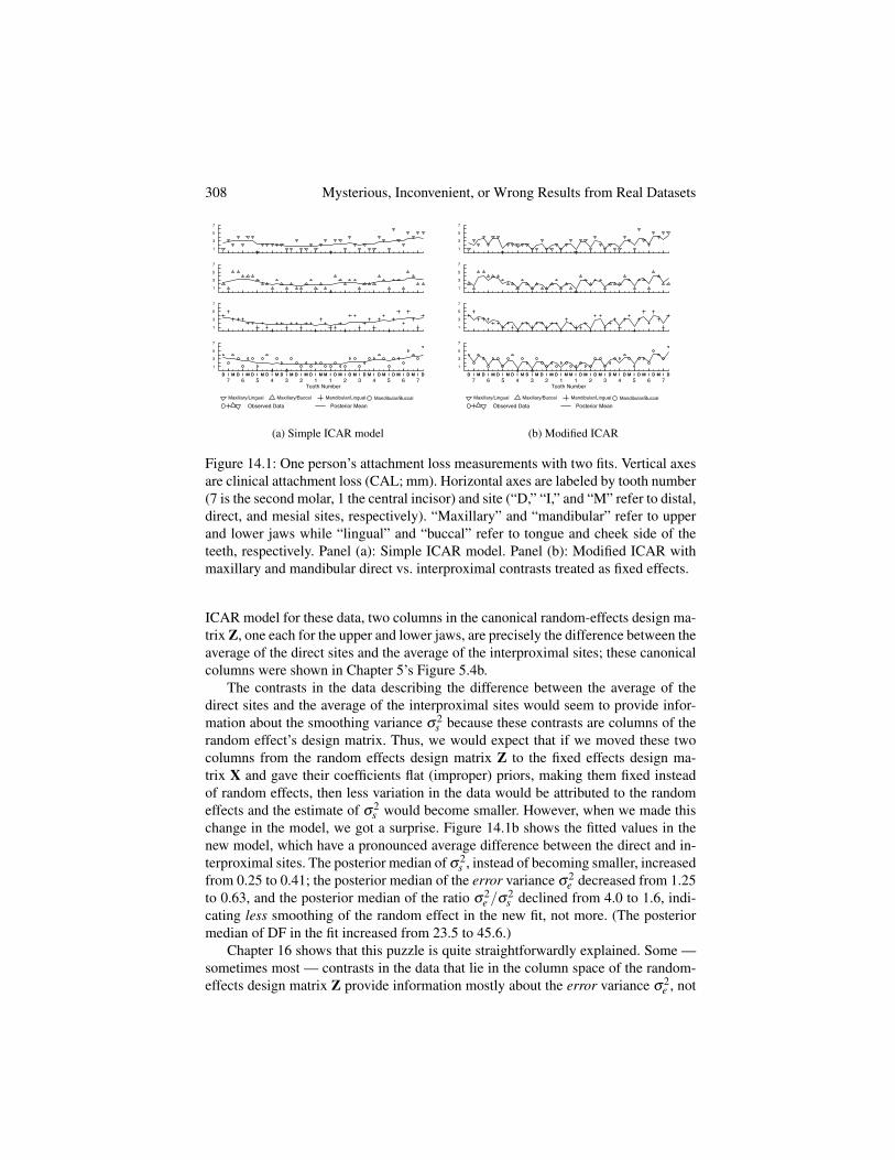
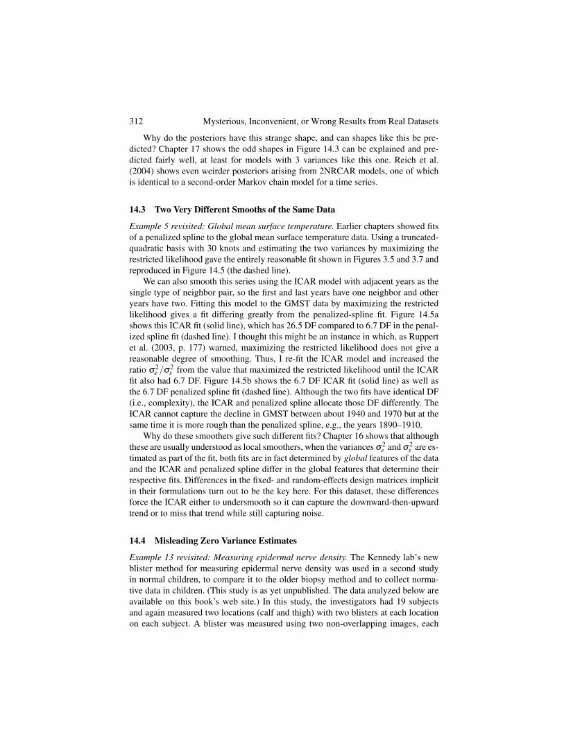
A diagnostic statistic suggested that the direct sites — the sites in the middle ofeach tooth, either on the lingual (tongue) or buccal (cheek) side of the tooth — tendto have lower attachment loss than their neighboring interproximal (distal or mesial)sites, especially for teeth farther back in the mouth. This tendency can be seen fairlyclearly in Figure 14.1a. For example, in the bottom echelon of the plot (the mandibu-lar buccal measurements), for the 6 teeth on the left of the plot the direct site isprominently lower than its neighbors. In the mixed-linear-model expression of the
1My colleague Bryan Michalowicz, a periodontologist, said of this fit, “I spend all my time worryingabout the 6 and 7 mm sites and you’re telling me I should ignore them and pay attention to this smoothline instead.” Um . . . no. This was our first fit to periodontal data; Reich & Hodges (2008b) gives a muchmore sensible analysis.
307
308 Mysterious, Inconvenient, or Wrong Results from Real DatasetsAt
tach
men
t Los
s (m
m)
Observed Data Posterior MeanMaxillary/Lingual Maxillary/Buccal Mandibular/Lingual Mandibular/Buccal
Tooth Number7 6 5 4 3 2 1 1 2 3 4 5 6 7
D | M D | M D | M D | M D | M D | M D | MD | M D | M D | M D | M D | M D | M D | M M | D M | D M | D M | D M | D M | D M | DM | D M | D M | D M | D M | D M | D M | D
1
3
5
7
1
3
5
7
1
3
5
7
1
3
5
7
(a) Simple ICAR modelAt
tach
men
t Los
s (m
m)
Observed Data Posterior MeanMaxillary/Lingual Maxillary/Buccal Mandibular/Lingual Mandibular/Buccal
Tooth Number7 6 5 4 3 2 1 1 2 3 4 5 6 7
D | M D | M D | M D | M D | M D | M D | MD | M D | M D | M D | M D | M D | M D | M M | D M | D M | D M | D M | D M | D M | DM | D M | D M | D M | D M | D M | D M | D
1
3
5
7
1
3
5
7
1
3
5
7
1
3
5
7
(b) Modified ICAR
Figure 14.1: One person’s attachment loss measurements with two fits. Vertical axesare clinical attachment loss (CAL; mm). Horizontal axes are labeled by tooth number(7 is the second molar, 1 the central incisor) and site (“D,” “I,” and “M” refer to distal,direct, and mesial sites, respectively). “Maxillary” and “mandibular” refer to upperand lower jaws while “lingual” and “buccal” refer to tongue and cheek side of theteeth, respectively. Panel (a): Simple ICAR model. Panel (b): Modified ICAR withmaxillary and mandibular direct vs. interproximal contrasts treated as fixed effects.
ICAR model for these data, two columns in the canonical random-effects design ma-trix Z, one each for the upper and lower jaws, are precisely the difference between theaverage of the direct sites and the average of the interproximal sites; these canonicalcolumns were shown in Chapter 5’s Figure 5.4b.
The contrasts in the data describing the difference between the average of thedirect sites and the average of the interproximal sites would seem to provide infor-mation about the smoothing variance s
2s because these contrasts are columns of the
random effect’s design matrix. Thus, we would expect that if we moved these twocolumns from the random effects design matrix Z to the fixed effects design ma-trix X and gave their coefficients flat (improper) priors, making them fixed insteadof random effects, then less variation in the data would be attributed to the randomeffects and the estimate of s
2s would become smaller. However, when we made this
change in the model, we got a surprise. Figure 14.1b shows the fitted values in thenew model, which have a pronounced average difference between the direct and in-terproximal sites. The posterior median of s
2s , instead of becoming smaller, increased
from 0.25 to 0.41; the posterior median of the error variance s
2e decreased from 1.25
to 0.63, and the posterior median of the ratio s
2e /s
2s declined from 4.0 to 1.6, indi-
cating less smoothing of the random effect in the new fit, not more. (The posteriormedian of DF in the fit increased from 23.5 to 45.6.)
Chapter 16 shows that this puzzle is quite straightforwardly explained. Some —sometimes most — contrasts in the data that lie in the column space of the random-effects design matrix Z provide information mostly about the error variance s
2e , not
Periodontal Data and the ICAR with Two Classes of Neighbor Pairs 309
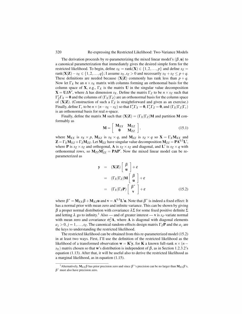
Type I
Type II
Type III
Type IV
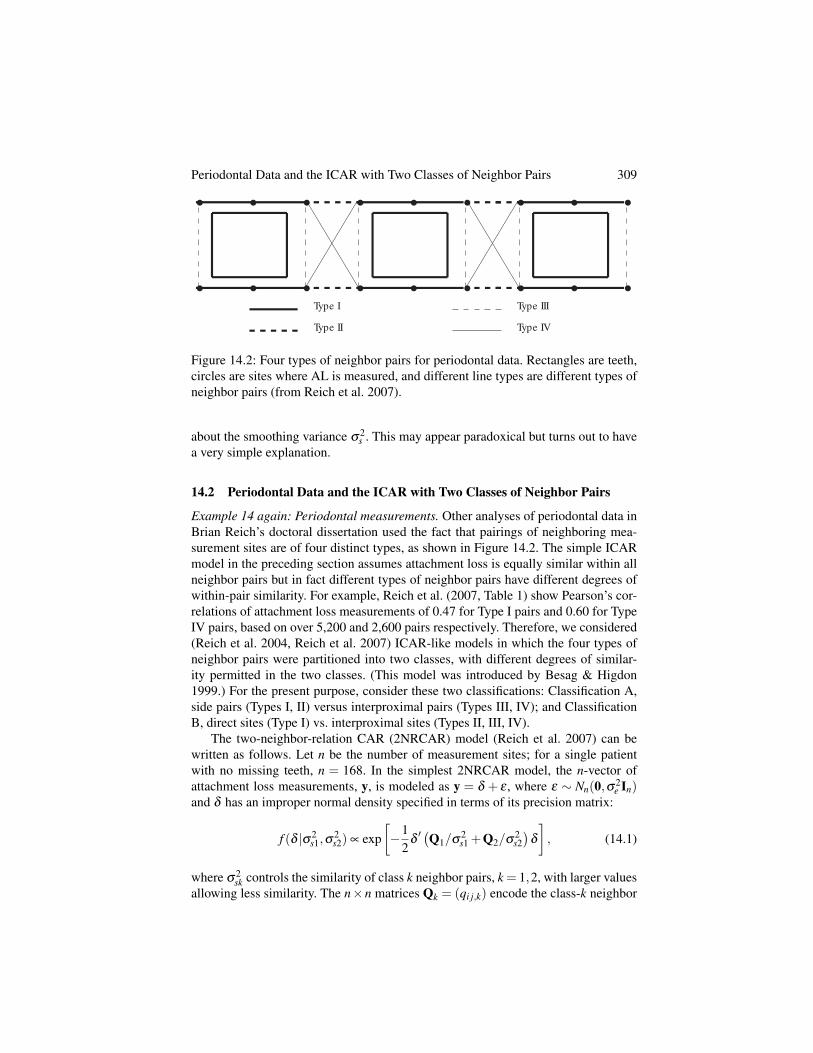
Figure 14.2: Four types of neighbor pairs for periodontal data. Rectangles are teeth,circles are sites where AL is measured, and different line types are different types ofneighbor pairs (from Reich et al. 2007).
about the smoothing variance s
2s . This may appear paradoxical but turns out to have
a very simple explanation.
14.2 Periodontal Data and the ICAR with Two Classes of Neighbor Pairs
Example 14 again: Periodontal measurements. Other analyses of periodontal data inBrian Reich’s doctoral dissertation used the fact that pairings of neighboring mea-surement sites are of four distinct types, as shown in Figure 14.2. The simple ICARmodel in the preceding section assumes attachment loss is equally similar within allneighbor pairs but in fact different types of neighbor pairs have different degrees ofwithin-pair similarity. For example, Reich et al. (2007, Table 1) show Pearson’s cor-relations of attachment loss measurements of 0.47 for Type I pairs and 0.60 for TypeIV pairs, based on over 5,200 and 2,600 pairs respectively. Therefore, we considered(Reich et al. 2004, Reich et al. 2007) ICAR-like models in which the four types ofneighbor pairs were partitioned into two classes, with different degrees of similar-ity permitted in the two classes. (This model was introduced by Besag & Higdon1999.) For the present purpose, consider these two classifications: Classification A,side pairs (Types I, II) versus interproximal pairs (Types III, IV); and ClassificationB, direct sites (Type I) vs. interproximal sites (Types II, III, IV).
The two-neighbor-relation CAR (2NRCAR) model (Reich et al. 2007) can bewritten as follows. Let n be the number of measurement sites; for a single patientwith no missing teeth, n = 168. In the simplest 2NRCAR model, the n-vector ofattachment loss measurements, y, is modeled as y = d + e , where e ⇠ Nn(0,s2
e In)and d has an improper normal density specified in terms of its precision matrix:
f (d |s2s1,s
2s2) µ exp
�1
2d
0 �Q1/s
2s1 +Q2/s
2s2�
d
�, (14.1)
where s
2sk controls the similarity of class k neighbor pairs, k = 1,2, with larger values
allowing less similarity. The n⇥n matrices Qk = (qi j,k) encode the class-k neighbor
310 Mysterious, Inconvenient, or Wrong Results from Real Datasets
pairs of measurement sites with qii,k being the number of site i’s class-k neighborsand qi j,k =�1 if sites i and j are class-k neighbors and 0 otherwise.
This model can be rewritten as a mixed linear model using the lemma (Newcomb1961) that there is a non-singular matrix B such that Qk = B0DkB, where Dk is diag-onal with non-negative diagonal elements. Dk has Ik zero diagonal elements, whereIk is the number of Qk’s zero eigenvalues and the number of islands in the spatialmap specified by Qk. Ik � I, where I is the number of zero eigenvalues of Q1 +Q2and also the number of zero diagonal entries in D1 +D2. B is non-singular but isorthogonal if and only if Q1Q2 is symmetric (Graybill 1983, Theorem 12.2.12).
Define v = Bd = (u0,b 0)0, where u and b have dimensions (n� I)⇥1 and I ⇥1respectively, and write B�1 = (Z|X), where Z is n⇥ (n� I) and X is n⇥ I. Becaused = B�1v, the model for y becomes y = d +e = Xb +Zu+e and the quadratic formin the exponent of equation (14.1) becomes
d
0 �Q1/s
2s1 +Q2/s
2s2�
d = v0�D1/s
2s1 +D2/s
2s2�
v= u0 �D1+/s
2s1 +D2+/s
2s2�
u (14.2)
where Dk+ is the upper-left (n� I)⇥(n� I) submatrix of Dk. The 2NRCAR model isnow a mixed linear model with random-effects covariance matrix G = (D1+/s
2s1 +
D2+/s
2s2)
�1. I have assumed and will continue to assume that the proportionalityconstant that’s missing in equation (14.1) is chosen by the same convention I haveused for the usual ICAR model since Section 5.2.2. As noted in that section, otherchoices also give legal probability distributions for u.
This model seemed straightforward enough. Because we thought it would sim-plify the MCMC, Prof. Reich put a Gamma(0.01,0.01) prior (mean 1, variance100) on 1/s
2e , derived the joint marginal posterior of the log variance ratios zk =
log(s2e /s
2sk), which control the shrinkage of class k neighbor pairs, and ran a
Metropolis-Hastings chain for (z1,z2). (Deriving this density is a special case ofChapter 1’s Regular Exercise 6 and is an exercise to the present chapter.) How-ever, despite extensive tinkering with the Metropolis-Hastings candidates, Prof. Re-ich found extremely high lagged autocorrelations in the MCMC series. I told himthere must be an error in his MCMC code, but he proved me wrong with contourplots of (z1,z2)’s log marginal posterior.
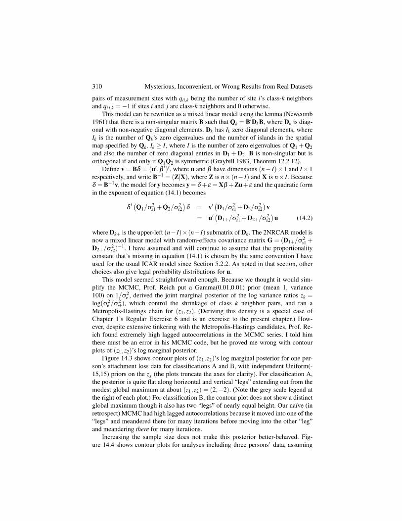
Figure 14.3 shows contour plots of (z1,z2)’s log marginal posterior for one per-son’s attachment loss data for classifications A and B, with independent Uniform(-15,15) priors on the z j (the plots truncate the axes for clarity). For classification A,the posterior is quite flat along horizontal and vertical “legs” extending out from themodest global maximum at about (z1,z2) = (2,�2). (Note the grey scale legend atthe right of each plot.) For classification B, the contour plot does not show a distinctglobal maximum though it also has two “legs” of nearly equal height. Our naıve (inretrospect) MCMC had high lagged autocorrelations because it moved into one of the“legs” and meandered there for many iterations before moving into the other “leg”and meandering there for many iterations.
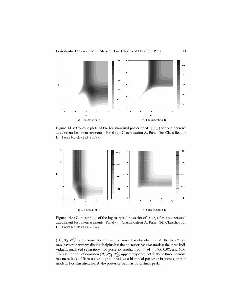
Increasing the sample size does not make this posterior better-behaved. Fig-ure 14.4 shows contour plots for analyses including three persons’ data, assuming
Periodontal Data and the ICAR with Two Classes of Neighbor Pairs 311
(a) Classification A (b) Classification B
Figure 14.3: Contour plots of the log marginal posterior of (z1,z2) for one person’sattachment loss measurements. Panel (a): Classification A. Panel (b): ClassificationB. (From Reich et al. 2007).
(a) Classification A (b) Classification B
Figure 14.4: Contour plots of the log marginal posterior of (z1,z2) for three persons’attachment loss measurements. Panel (a): Classification A. Panel (b): ClassificationB. (From Reich et al. 2004).
(s2e ,s
2s1,s
2s2) is the same for all three persons. For classification A, the two “legs”
now have rather more distinct heights but the posterior has two modes; the three indi-viduals, analyzed separately, had posterior medians for z2 of �1.75, 0.08, and 6.09.The assumption of common (s2
e ,s2s1,s
2s2) apparently does not fit these three persons,
but mere lack of fit is not enough to produce a bi-modal posterior in most commonmodels. For classification B, the posterior still has no distinct peak.
312 Mysterious, Inconvenient, or Wrong Results from Real Datasets
Why do the posteriors have this strange shape, and can shapes like this be pre-dicted? Chapter 17 shows the odd shapes in Figure 14.3 can be explained and pre-dicted fairly well, at least for models with 3 variances like this one. Reich et al.(2004) shows even weirder posteriors arising from 2NRCAR models, one of whichis identical to a second-order Markov chain model for a time series.
14.3 Two Very Different Smooths of the Same Data
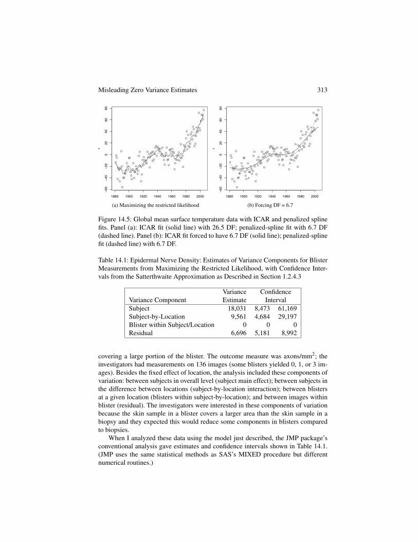
Example 5 revisited: Global mean surface temperature. Earlier chapters showed fitsof a penalized spline to the global mean surface temperature data. Using a truncated-quadratic basis with 30 knots and estimating the two variances by maximizing therestricted likelihood gave the entirely reasonable fit shown in Figures 3.5 and 3.7 andreproduced in Figure 14.5 (the dashed line).
We can also smooth this series using the ICAR model with adjacent years as thesingle type of neighbor pair, so the first and last years have one neighbor and otheryears have two. Fitting this model to the GMST data by maximizing the restrictedlikelihood gives a fit differing greatly from the penalized-spline fit. Figure 14.5ashows this ICAR fit (solid line), which has 26.5 DF compared to 6.7 DF in the penal-ized spline fit (dashed line). I thought this might be an instance in which, as Ruppertet al. (2003, p. 177) warned, maximizing the restricted likelihood does not give areasonable degree of smoothing. Thus, I re-fit the ICAR model and increased theratio s
2e /s
2s from the value that maximized the restricted likelihood until the ICAR
fit also had 6.7 DF. Figure 14.5b shows the 6.7 DF ICAR fit (solid line) as well asthe 6.7 DF penalized spline fit (dashed line). Although the two fits have identical DF(i.e., complexity), the ICAR and penalized spline allocate those DF differently. TheICAR cannot capture the decline in GMST between about 1940 and 1970 but at thesame time it is more rough than the penalized spline, e.g., the years 1890–1910.
Why do these smoothers give such different fits? Chapter 16 shows that althoughthese are usually understood as local smoothers, when the variances s
2e and s
2s are es-
timated as part of the fit, both fits are in fact determined by global features of the dataand the ICAR and penalized spline differ in the global features that determine theirrespective fits. Differences in the fixed- and random-effects design matrices implicitin their formulations turn out to be the key here. For this dataset, these differencesforce the ICAR either to undersmooth so it can capture the downward-then-upwardtrend or to miss that trend while still capturing noise.
14.4 Misleading Zero Variance Estimates
Example 13 revisited: Measuring epidermal nerve density. The Kennedy lab’s newblister method for measuring epidermal nerve density was used in a second studyin normal children, to compare it to the older biopsy method and to collect norma-tive data in children. (This study is as yet unpublished. The data analyzed below areavailable on this book’s web site.) In this study, the investigators had 19 subjectsand again measured two locations (calf and thigh) with two blisters at each locationon each subject. A blister was measured using two non-overlapping images, each
Misleading Zero Variance Estimates 313
1880 1900 1920 1940 1960 1980 2000
−60
−40
−20
020
4060
80
Year
y
(a) Maximizing the restricted likelihood
1880 1900 1920 1940 1960 1980 2000
−60
−40
−20
020
4060
80
Year
y
(b) Forcing DF = 6.7
Figure 14.5: Global mean surface temperature data with ICAR and penalized splinefits. Panel (a): ICAR fit (solid line) with 26.5 DF; penalized-spline fit with 6.7 DF(dashed line). Panel (b): ICAR fit forced to have 6.7 DF (solid line); penalized-splinefit (dashed line) with 6.7 DF.
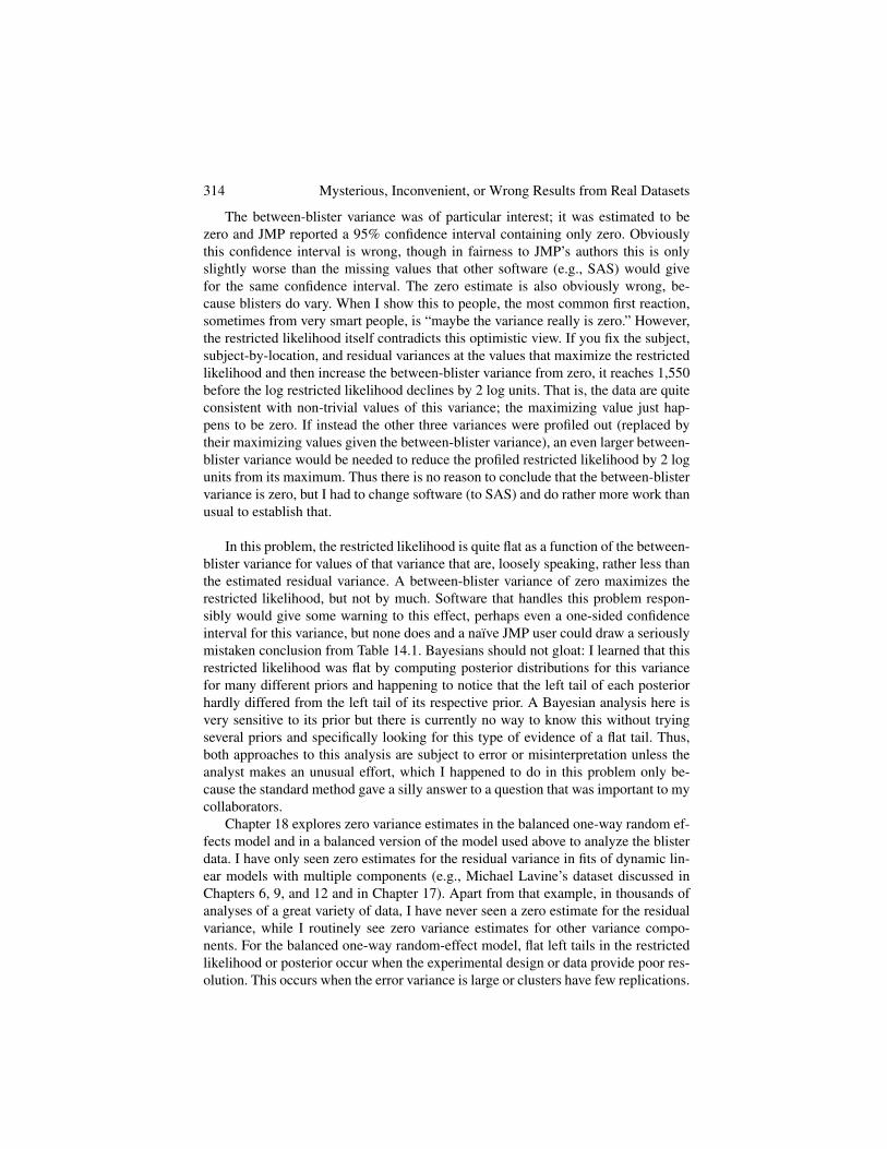
Table 14.1: Epidermal Nerve Density: Estimates of Variance Components for BlisterMeasurements from Maximizing the Restricted Likelihood, with Confidence Inter-vals from the Satterthwaite Approximation as Described in Section 1.2.4.3
Variance ConfidenceVariance Component Estimate IntervalSubject 18,031 8,473 61,169Subject-by-Location 9,561 4,684 29,197Blister within Subject/Location 0 0 0Residual 6,696 5,181 8,992
covering a large portion of the blister. The outcome measure was axons/mm2; theinvestigators had measurements on 136 images (some blisters yielded 0, 1, or 3 im-ages). Besides the fixed effect of location, the analysis included these components ofvariation: between subjects in overall level (subject main effect); between subjects inthe difference between locations (subject-by-location interaction); between blistersat a given location (blisters within subject-by-location); and between images withinblister (residual). The investigators were interested in these components of variationbecause the skin sample in a blister covers a larger area than the skin sample in abiopsy and they expected this would reduce some components in blisters comparedto biopsies.
When I analyzed these data using the model just described, the JMP package’sconventional analysis gave estimates and confidence intervals shown in Table 14.1.(JMP uses the same statistical methods as SAS’s MIXED procedure but differentnumerical routines.)
314 Mysterious, Inconvenient, or Wrong Results from Real Datasets
The between-blister variance was of particular interest; it was estimated to bezero and JMP reported a 95% confidence interval containing only zero. Obviouslythis confidence interval is wrong, though in fairness to JMP’s authors this is onlyslightly worse than the missing values that other software (e.g., SAS) would givefor the same confidence interval. The zero estimate is also obviously wrong, be-cause blisters do vary. When I show this to people, the most common first reaction,sometimes from very smart people, is “maybe the variance really is zero.” However,the restricted likelihood itself contradicts this optimistic view. If you fix the subject,subject-by-location, and residual variances at the values that maximize the restrictedlikelihood and then increase the between-blister variance from zero, it reaches 1,550before the log restricted likelihood declines by 2 log units. That is, the data are quiteconsistent with non-trivial values of this variance; the maximizing value just hap-pens to be zero. If instead the other three variances were profiled out (replaced bytheir maximizing values given the between-blister variance), an even larger between-blister variance would be needed to reduce the profiled restricted likelihood by 2 logunits from its maximum. Thus there is no reason to conclude that the between-blistervariance is zero, but I had to change software (to SAS) and do rather more work thanusual to establish that.
In this problem, the restricted likelihood is quite flat as a function of the between-blister variance for values of that variance that are, loosely speaking, rather less thanthe estimated residual variance. A between-blister variance of zero maximizes therestricted likelihood, but not by much. Software that handles this problem respon-sibly would give some warning to this effect, perhaps even a one-sided confidenceinterval for this variance, but none does and a naıve JMP user could draw a seriouslymistaken conclusion from Table 14.1. Bayesians should not gloat: I learned that thisrestricted likelihood was flat by computing posterior distributions for this variancefor many different priors and happening to notice that the left tail of each posteriorhardly differed from the left tail of its respective prior. A Bayesian analysis here isvery sensitive to its prior but there is currently no way to know this without tryingseveral priors and specifically looking for this type of evidence of a flat tail. Thus,both approaches to this analysis are subject to error or misinterpretation unless theanalyst makes an unusual effort, which I happened to do in this problem only be-cause the standard method gave a silly answer to a question that was important to mycollaborators.
Chapter 18 explores zero variance estimates in the balanced one-way random ef-fects model and in a balanced version of the model used above to analyze the blisterdata. I have only seen zero estimates for the residual variance in fits of dynamic lin-ear models with multiple components (e.g., Michael Lavine’s dataset discussed inChapters 6, 9, and 12 and in Chapter 17). Apart from that example, in thousands ofanalyses of a great variety of data, I have never seen a zero estimate for the residualvariance, while I routinely see zero variance estimates for other variance compo-nents. For the balanced one-way random-effect model, flat left tails in the restrictedlikelihood or posterior occur when the experimental design or data provide poor res-olution. This occurs when the error variance is large or clusters have few replications.

Multiple Maxima in Posteriors and Restricted Likelihoods 315
The situation is more complicated for designs with more components of variance al-though broadly speaking it seems that the problem is still poor resolution. Chapter 18briefly considers some approaches to diagnostics for a flat left tail.
14.5 Multiple Maxima in Posteriors and Restricted Likelihoods
Example 9 revisited: HMO premium data. Section 5.2 of Hodges (1998) reportedan analysis of the HMO premium data using two state-level predictors suggested bythat paper’s diagnostics, state average expenses per hospital admission (centered andscaled) and an indicator for the New England states. As in the analyses described inChapter 8, I used a flat prior on the fixed effects, a flat prior on 1/s
2e (which I would
not do now), and “a low information gamma prior for [1/s
2s ], with mean 11 and
variance 110.” I described my 1000-iteration Gibbs sampler output2 by saying, “TheGibbs sampler was unstable through about 250 iterations; from iteration 251 to 1000the sampler provided satisfactory convergence diagnostics, and these [750] iterationswere used for the computations that follow.” “Unstable” refers to the trace plot fors
2s , which was stable for the first 250 iterations then dropped to a distinctly lower
level, where it was stable for the remaining 750 iterations. Such behavior meansthe posterior is bimodal but when I did this analysis I had never entertained thepossibility that this posterior might have two modes.
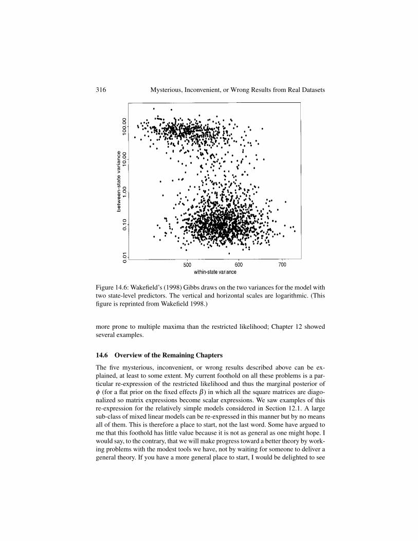
Wakefield’s discussion of this paper (Wakefield 1998) touched on several top-ics before re-running the above analysis with 10,000 Gibbs iterations. Figure 14.6,Wakefield’s scatter plot of the Gibbs draws on the two variances, clearly shows theposterior’s two modes, one with tiny s
2s (between-state variance) and one with rather
large s
2s ; the former has more mass than the latter. Wakefield commented that the
bimodal posterior showed “there are two competing explanations for the observedvariability in the data” (p. 525).
This was embarrassing, as you can imagine, but I was naıve and deserved it,and Wakefield exposed my error as gently as possible. My next PhD student, Jian-nong Liu, studied bimodality in mixed linear models; Chapter 19 summarizes hisresults (Liu & Hodges 2003), among others. I hope it does not seem churlish whenChapter 19 shows that the mode with more mass in Figure 14.6 is not present in therestricted likelihood but arises entirely from the prior on 1/s
2s . Thus, it is not quite
true that “there are two competing explanations for the observed variability in thedata”; rather, the data’s information about s
2s is weak enough to be punctured easily
by a thoughtlessly chosen prior.Bimodal posteriors arising from a strong prior are not mysterious but they can be
inconvenient and given that many priors are chosen by convention without carefulsubstantive consideration, in a given problem one might decide that a bimodal pos-terior is wrong. Anti-Bayesians should not gloat: The restricted likelihood itself canhave more than one maximum and as we have seen, even when it has a single max-imum that is not necessarily a sensible estimate. The likelihood appears to be even
2I now know that such a short run is malpractice, but I didn’t know it then and oddly, none of thereferees pointed it out although one of the discussants did.
316 Mysterious, Inconvenient, or Wrong Results from Real Datasets
Figure 14.6: Wakefield’s (1998) Gibbs draws on the two variances for the model withtwo state-level predictors. The vertical and horizontal scales are logarithmic. (Thisfigure is reprinted from Wakefield 1998.)
more prone to multiple maxima than the restricted likelihood; Chapter 12 showedseveral examples.
14.6 Overview of the Remaining Chapters
The five mysterious, inconvenient, or wrong results described above can be ex-plained, at least to some extent. My current foothold on all these problems is a par-ticular re-expression of the restricted likelihood and thus the marginal posterior off (for a flat prior on the fixed effects b ) in which all the square matrices are diago-nalized so matrix expressions become scalar expressions. We saw examples of thisre-expression for the relatively simple models considered in Section 12.1. A largesub-class of mixed linear models can be re-expressed in this manner but by no meansall of them. This is therefore a place to start, not the last word. Some have argued tome that this foothold has little value because it is not as general as one might hope. Iwould say, to the contrary, that we will make progress toward a better theory by work-ing problems with the modest tools we have, not by waiting for someone to deliver ageneral theory. If you have a more general place to start, I would be delighted to see

Overview of the Remaining Chapters 317
it. As far as I can tell, however, nobody has yet developed such a general theory, so Ipresent this modest beginning for what it may be worth.
This book’s remaining chapters develop and use the re-expressed restricted likeli-hood, proceeding as follows. Chapter 15 introduces the re-expression for a small butinteresting sub-class of mixed linear models called two-variance models and appliesit to penalized splines, ICAR models, and a dynamic linear model with one quasi-cyclic component. Chapter 15 also introduces some analytic tools derived using there-expression. Chapter 16 uses this re-expression to examine which functions of thedata provide information about the smoothing and error variances in a two-variancemodel and applies the results to penalized splines and ICAR models to explain thefirst two mysteries discussed above. Chapter 17 extends the re-expression to modelsthat are more general than two-variance models. I cannot explicitly characterize theclass of models for which the re-expression can be done, but this chapter proves thatit cannot be done for all mixed linear models though useful extensions might be pos-sible, as suggested at the end of Chapter 12. Chapter 17 chapter gives two expedientsthat can be used for some models that cannot be re-expressed in the diagonalizedform, one of which allows us to explain the third mystery, for 2NRCAR models.Chapter 18 uses the re-expressed restricted likelihood for an as-yet too brief consid-eration of zero variance estimates, while Chapter 19 uses it to examine multiple localmaxima in the restricted likelihood and marginal posterior.
Two other problems would fit here in Part IV but so far I do not even have afoothold on explanations for them. These problems were mentioned in connectionwith Chapter 1’s Example 2 (vocal folds) and Example 3 (glomerular filtration rate).Example 2 exhibited unpredictable convergence of numerical algorithms, which isinconvenient and currently mysterious. Example 3 exhibited unpredictable conver-gence and also correlation estimates of ±1, which are inconvenient and wrong. Es-timates of ±1 are somewhat like zero variance estimates but as yet I have no insightinto why they occur. I guess they are more complicated than zero variance estimates,which (Chapter 18 argues) generally arise from poor resolution in the data or design,but that is only a guess.
Regarding unpredictable convergence, one reader noted that the solution maysimply be a smarter optimization algorithm or running the same optimization routinemany times with different starting values. The latter is certainly the sensible thing todo when you encounter this problem. However, if we really understood our mixed-linear-model tools, it would be possible to determine which aspects of the data anddesign cause the restricted likelihood or posterior to be ill-behaved and perhaps toavoid the difficulty by using a different design or by selecting a numerical algorithmmore suited to the problem.
Bad behavior of this sort is fairly well understood for generalized linear mod-els. For example, we know we’ll have convergence problems with a logistic regres-sion if a categorical predictor has a category in which all the outcomes are either“No” or “Yes.” Wedderburn (1976, p. 31)3 gave a catalog of generalized linear mod-els organized by error distribution and link function, identifying which models give
3Thanks to Lisa Henn for pointing out this under-appreciated gem.

318 Mysterious, Inconvenient, or Wrong Results from Real Datasets
maximum-likelihood estimates that are finite or unique or in the parameter space’sinterior. Ideally, a similar catalog could be constructed for mixed linear models orat least a large subset of them. This is too much to hope for now, of course, but thefollowing chapters may suggest a place to start.
Exercises
Regular Exercises
1. (Section 14.2). Derive the joint marginal posterior of (z1,z2) in the 2NRCARmodel, for the assumptions used in Section 14.2. Use a gamma prior for s
2e and
an independent and non-specific prior p(z1,z2) for (z1,z2).
Open Questions
1. (Introduction to Part IV) Prove that for the balanced one-way random-effectsmodel, no function of the data y has a distribution that depends on the between-group variance s
2s but not the within-group variance s
2s . This is easy to show for
linear functions of y and for a second-order approximation to an arbitrary con-tinuous function, but I haven’t been able to show it for more general functions.Are there functions of the data that depend on s
2e /s
2s but not on either variance
individually?2. Re-analyze the available datasets from this chapter to see whether you can figure
out why the mysterious, inconvenient, or wrong results happened, before you readthe following chapters and see what my colleagues and I did.
Chapter 15
Re-expressing the RestrictedLikelihood: Two-Variance Models
This chapter and the next consider two-variance models, which can be defined asmodels in mixed-linear-model form (1.1) with R = s
2e Se and G = s
2s Ss for known
Se and Ss and unknown s
2e and s
2s . I assume Se and Ss are positive definite, though
this may not be necessary. For every model in this class, the restricted likelihood canbe re-expressed in a simple form that this chapter and the next develop and explore.Chapter 17 extends this re-expression to a larger class of models. The class of two-variance models may seem small but it includes examples of most models consideredin Part II of this book (not additive models) and its simplicity permits considerableinsight.
In this chapter, the re-expressed restricted likelihood is derived for two-variancemodels, its key features are identified, and it is shown to be identical to a par-ticular generalized linear model. The re-expression involves a rather obscure re-parameterization so it is then applied to several examples, for which the re-parameterization is more or less interpretable. The chapter concludes by introducingsome tools based on the re-expression.
15.1 The Re-expression
As far as I know, this re-expression was first presented by Reich & Hodges (2008a)and independently presented for a special case by Welham & Thompson (2009),though it generalizes a representation used in analysis of variance (McCullagh &Nelder 1989, Section 8.3.5). Reich & Hodges (2008a) expressed two-variance mod-els in a hierarchical form using precision matrices. Their re-expression is the sameas the one given below, which begins with two-variance models expressed in mixed-linear-model form. Besides being consistent with the rest of this book, the derivationbelow avoids some untidy aspects of the derivation in Reich & Hodges (2008a) andthus supersedes it.
First, in the definition of two-variance models given above, without loss of gen-erality set Se = In and Ss = Iq. If Se is not the identity, the data y can be transformedto S�0.5
e y so the transformed problem has Se = In. Similarly, if Ss is not the identity,the random effects can be re-parameterized as Zu = Z⇤u⇤ with u⇤ = S�0.5
s u, whichhas covariance proportional to the identity.
319
320 Re-expressing the Restricted Likelihood: Two-Variance Models
The derivation proceeds by re-parameterizing the mixed linear model’s (b ,u) toa canonical parameterization that immediately gives the desired simple form for therestricted likelihood. To begin, define sX = rank(X) 2 {1,2, . . . , p} and define sZ =rank(X|Z)� sX 2 {1,2, . . . ,q}; I assume sX ,sZ > 0 and necessarily sX + sZ p+q.These definitions are needed because (X|Z) commonly has rank less than p + q.Now let GX be an n⇥ sX matrix with columns forming an orthonomal basis for thecolumn space of X, e.g., GX is the matrix U in the singular value decompositionX = UDV0, where D has dimension sX . Define the matrix GZ to be n⇥ sZ such thatG0
ZGX = 0 and the columns of (GX |GZ) are an orthonormal basis for the column spaceof (X|Z). (Construction of such a GZ is straightforward and given as an exercise.)Finally, define Gc to be n⇥(n�sX �sZ) so that G0
cGX = 0, G0cGZ = 0, and (GX |GZ |Gc)
is an orthonormal basis for real n-space.Finally, define the matrix M such that (X|Z) = (GX |GZ)M and partition M con-
formably as
M =
MXX MXZ
0 MZZ
�, (15.1)
where MXX is sX ⇥ p, MXZ is sX ⇥ q, and MZZ is sZ ⇥ q so X = GX MXX andZ = GX MXZ +GZMZZ . Let MZZ have singular value decomposition MZZ = PA0.5L0,where P is sZ ⇥ sZ and orthogonal, A is sZ ⇥ sZ and diagonal, and L0 is sZ ⇥ q withorthonormal rows, so MZZM0
ZZ = PAP0. Now the mixed linear model can be re-parameterized as
y = (X|Z)
b
u
�+ e
= (GX |GZ)M
b
u
�+ e
= (GX |GZP)
b
⇤
v
�+ e (15.2)
where b
⇤ = MXX b +MXZu and v = A0.5L0u. Note that b
⇤ is indeed a fixed effect: Ithas a normal prior with mean zero and infinite variance. This can be shown by givingb a proper normal distribution with covariance lS for some fixed positive definite Sand letting l go to infinity.1 Also — and of greater interest — v is sZ-variate normalwith mean zero and covariance s
2s A, where A is diagonal with diagonal elements
a j > 0, j = 1, . . . ,sZ . The canonical random-effects design matrix GZP and the a j arethe keys to understanding the restricted likelihood.
The restricted likelihood can be obtained from this re-parameterized model (15.2)in at least two ways. First, I’ll use the definition of the restricted likelihood as thelikelihood of a transformed observation w = K0y, for K a known full-rank n⇥ (n�sX ) matrix chosen so that w’s distribution is independent of b , as in Section 1.2.3.2’sequation (1.13). After that, it will be useful also to derive the restricted likelihood asa marginal likelihood, as in equation (1.15).
1Alternatively, MXX b has prior precision zero and since b
⇤’s precision can be no larger than MXX b ’s,b
⇤ must also have precision zero.
The Re-expression 321
In the first definition of the restricted likelihood, define K = (GZP|Gc). Pre-multiply equation (15.2) by K0 to give
w = K0y =
v
0(n�sX�sZ)⇥1
�+x , (15.3)
where x ⇠ N(0,s2e In�sX ) and, as before, v ⇠ NsZ (0,s2
s A). The log restricted likeli-hood for (s2
s ,s2e ) is the log likelihood arising from (15.3):
logRL(s2s ,s
2e |y) = B� n� sX � sZ
2log(s2
e )�1
2s
2e
y0GcG0cy
�12
sZ
Âj=1
"log(s2
s a j +s
2e )+
v2j
s
2s a j +s
2e
#, (15.4)
for B an unimportant constant and v = (v1, . . . , vsZ )0 = P0G0
Zy. Note that y0GcG0cy is
the residual sum of squares from the simple linear model with outcome y and designmatrix (X|Z), or equivalently from a fit of the mixed linear model with s
2s = •. I call
this the unshrunk fit of y on (X|Z) because the u are not shrunk toward zero. Also, vis a known linear function of y, the estimate of v in a fit of model (15.2) with s
2s = •,
which I’ll call the unshrunk estimate of v. The v j capture the information in the datathat is specific to the model’s random effects, that is, not confounded with the fixedeffects.
The choice of GZ would appear to affect the v j, but in fact (15.4) is invariant tothe choice of GZ . (The proof is straightforward and given as an exercise.) If some a jhas multiplicity greater than 1, the terms in ÂsZ
j=1 v2j(s
2s a j +s
2e )
�1 having the samea j become (s2
s a j +s
2e )
�1 Âk v2k , and Âk v2
k is invariant to the choice of GZ .Two comments: Note that y0GcGcy = y0(In � X(X0X)�1X0)y + ÂsZ
j=1 v2j , where
y0(In�X(X0X)�1X0)y is the residual sum of squares for a fit of y on X only, i.e., a fitof the mixed linear model in which the random effects u are shrunk to 0. This allows(15.4) to be rewritten in terms of the precisions 1/s
2e and 1/s
2s , possibly to some
advantage. Also, note the importance of the flat prior on b . If b is instead given aproper normal prior, this becomes a three-variance model even if that proper prior hasno unknowns, and the marginal posterior of (s2
s ,s2e ) has a simple form like (15.4)
only under certain conditions on X and Z.It is useful also to derive the restricted likelihood as a marginal likelihood. Begin
with (15.2) and pre-multiply both sides of the equation by (GX |GZP|Gc)0 to give2
4G0
XP0G0
ZG0
c
3
5y =
2
4IsX 00 IsZ0 0
3
5
b
⇤
v
�+ e, (15.5)
where as before v ⇠ NsZ (0,s2s A) and the distribution of e is unchanged because
the equation was pre-multiplied by an orthogonal matrix. If p(s2e ,s
2s ) is the prior
distribution for (s2e ,s
2s ), the joint posterior distribution of all the unknowns is easily
322 Re-expressing the Restricted Likelihood: Two-Variance Models
shown to be
p(b ⇤,v,s2e ,s
2s |y) µ p(s2
e ,s2s )
(s2e )
�sX/2 exp��(b ⇤ �G0
X y)0(b ⇤ �G0X y)/2s
2e�
(15.6)sZ
’j=1
✓s
2e
a j
a j + r
◆�0.5exp
�
sZ
Âj=1
✓2s
2e
a j
a j + r
◆�1(v j � v j)
2
!
(15.7)(s2
e )�(n�sX�sZ)/2 exp
��y0GcG0
cy/2s
2e�
(15.8)sZ
’j=1
�s
2s a j +s
2e��0.5 exp
�
sZ
Âj=1
v2j/2(s2
s a j +s
2e )
!, (15.9)
where v j =a j
a j+r v j and r = s
2e /s
2s , as usual. (The proof is an exercise.) Equation
(15.6) is the conditional posterior of the re-parameterized fixed effects, b
⇤, given(s2
e ,s2s ). Equation (15.7) is the conditional posterior of the re-parameterized ran-
dom effects, v, given (s2e ,s
2s ). Conditionally, the v j are independent with mean v j,
variance s
2e a j/(a j + r), and DF a j/(a j + r). Thus given r = s
2e /s
2s , v j is shrunk
more for j with smaller a j. Integrating (15.6) and (15.7) out of this joint posteriorleaves (15.8) and (15.9); they are the re-expressed restricted likelihood as in (15.4).
It is convenient to break the log restricted likelihood (15.4) into two pieces. Thefirst piece, �(n� sX � sZ) log(s2
e )/2� y0GcG0cy/2s
2e , is a function only of s
2e and
will be called the free terms for s
2e because it is free of s
2s . The second piece is
�12
sZ
Âj=1
"log(s2
s a j +s
2e )+
v2j
s
2s a j +s
2e
#, (15.10)
which will be called mixed terms because each summand (mixed term) involves bothvariances. As we will see, the free terms are absent for some models, e.g., a modelincluding an ICAR random effect. When present, they provide strong informationabout s
2e , information that is in a sense uncontaminated by information about s
2s .
The data’s information about s
2s enters the restricted likelihood entirely through the
mixed terms and is thus always mixed with information about s
2e .
Several features make this re-expression interpretable and useful. First, the v j areknown functions of the data; whenever the fixed effects include an intercept, they arecontrasts in the data. Second, the form of (15.4) implies that the v j are independentconditional on (s2
e ,s2s ); that’s why the restricted likelihood decomposes in this sim-
ple way. (The following paragraph gives another way to see this.) In particular, theconditional distribution of v j given (s2
e ,s2s ) is normal with mean zero and variance
s
2s a j +s
2e , a simple linear function of the unknown variances. This means the a j —
which are functions of the design matrices X and Z, albeit obscure ones at this point— determine how the canonical “observations” v j and y0GcG0
cy provide informationabout s
2e and s
2s and do so in a fairly simple way that is explored in this and the next
chapter. Third, the v j are independent a posteriori conditional on (s2e ,s
2s ) and have
simple conditional posterior mean, variance, and DF. Finally, by assumption sZ > 0
Examples 323
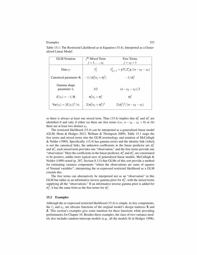
Table 15.1: The Restricted Likelihood as in Equation (15.4), Interpreted as a Gener-alized Linear Model
GLM Notation jth Mixed Term Free Termsj = 1, . . . ,sZ j = sZ +1
Data yi v2j v2
sZ+1 = y0GcG0cy/(n� sX � sZ)
Canonical parameter qi �1/(s2s a j +s
2e ) �1/s
2e
Gamma shapeparameter ni 1/2 (n� sX � sZ)/2
E(yi) =�1/qi s
2s a j +s
2e s
2e
Var(yi) = [E(yi)]2/ni 2(s2s a j +s
2e )
2 2(s2e )
2/(n� sX � sZ)
so there is always at least one mixed term. Thus (15.4) implies that s
2e and s
2s are
identified if and only if either (a) there are free terms (i.e., n� sX � sZ > 0) or (b)there are at least two distinct a j.
The restricted likelihood (15.4) can be interpreted as a generalized linear model(GLM; Henn & Hodges 2013, Welham & Thompson 2009). Table 15.1 maps thefree terms and mixed terms into the GLM terminology and notation of McCullagh& Nelder (1989). Specifically, (15.4) has gamma errors and the identity link (whichis not the canonical link), the unknown coefficients in the linear predictor are s
2e
and s
2s , each mixed term provides one “observation,” and the free terms provide one
“observation.” Here the coefficients in the linear predictor, s
2e and s
2s , are constrained
to be positive, unlike more typical uses of generalized linear models. McCullagh &Nelder (1989) noted (p. 287, Section 8.3.5) that GLMs of this sort provide a methodfor estimating variance components “where the observations are sums of squaresof Normal variables”; interpreting the re-expressed restricted likelihood as a GLMextends this.
The free terms can alternatively be interpreted not as an “observation” in thisGLM but rather as an informative inverse gamma prior for s
2e , with the mixed terms
supplying all the “observations.” If an informative inverse gamma prior is added fors
2s , it has the same form as the free terms for s
2e .
15.2 Examples
Although the re-expressed restricted likelihood (15.4) is simple, its key components,the v j and a j, are obscure functions of the original model’s design matrices X andZ. This section’s examples give some intuition for these functions while providingpreliminaries for Chapter 16. Besides these examples, the class of two-variance mod-els also includes random-intercept models (e.g., all the models fit in Hodges 1998),
324 Re-expressing the Restricted Likelihood: Two-Variance Models
multiple-membership models (e.g., Browne et al. 2001, McCaffrey et al. 2004), andno doubt others.
15.2.1 Balanced One-Way Random Effect Model
The balanced one-way random effect model can be written as yi j = b0 +ui + ei j fori = 1, . . . ,N and j = 1, . . . ,m, ui ⇠ N(0,s2
s ) and ei j ⇠ N(0,s2e ). Order the obser-
vations in y with j varying fastest, as y = (y11, . . . ,y1m,y21, . . . ,yNm)0. Then in themixed-linear-model form, n = Nm, X = 1n, Z = IN ⌦1m, where the Kronecker prod-uct ⌦ is defined for matrices A = (ai j) and B as A⌦B = (ai jB), G = s
2s IN , and
R = s
2e INm. X = Z1N , so sZ = N �1 while sX = 1.
The matrix GX in the re-expression is 1pn 1n. GZ can be any matrix of the form
F⌦ 1pm 1m where F is N ⇥ (N � 1) satisfying F0F = IN�1, i.e., F’s columns are an
orthonormal basis for the orthogonal complement of 1N . Then MZZ = G0ZZ =
pmF0,
so MZZM0ZZ = mIN�1, a j = m, j = 1, . . . ,N � 1, and P is IN�1. Finally, v = G0
Zy sov0 =
pm(y1., . . . , yN.)F, where yi. = Â j yi j/m is the average of group i’s observations.
Plugging all this into the re-expressed log restricted likelihood (15.4) gives thefamiliar form
�n�N2
log(s2e )�
12s
2e
Âi, j(yi j � yi.)
2 � N �12
log(s2s m+s
2e )
�m2 Â
i(yi.� y..)2/(s2
s m+s
2e ), (15.11)
where y.. = Âi j yi j/n is the average of all n = Nm observations. Because there is onlyone distinct a j, the two variances are identified if and only if n > N, i.e., m > 1,not exactly a novel finding. Interpreted as a GLM with unknown coefficients s
2s and
s
2e , this GLM has two “observations,” with one each arising from the residual and
between-group mean squares.
15.2.2 Penalized Spline
Example 5 again, global mean surface temperature. Consider yet again the pe-nalized spline fit to this dataset in several previous chapters. The dataset has n =125 observation. The spline has a truncated quadratic basis and 30 knots at years1880+ {4, . . . ,120}. The predictor (year) and knots are centered and scaled as be-fore. The fixed-effects design matrix X has sX = p = 3 columns for the intercept, lin-ear, and quadratic terms, while the random-effects design matrix Z has sZ = q = 30columns, one for each knot. The combined design matrix (X|Z) has rank 33 thoughit is very close to rank-deficient: The first canonical correlation of X and Z is greaterthan 0.99999995.
Table 15.2 lists the eigenvalues a j in the restricted likelihood’s re-expression.The a j decline quickly: a1/a6 = 1841, and the last 18 a j are all smaller than a1 bya factor of at least 100,000. In Chapter 16 we will see that this rapid decline in thea j implies that the first few v j provide almost all of the information in the data abouts
2s , with the remaining v j providing information almost exclusively about s
2e .
Examples 325
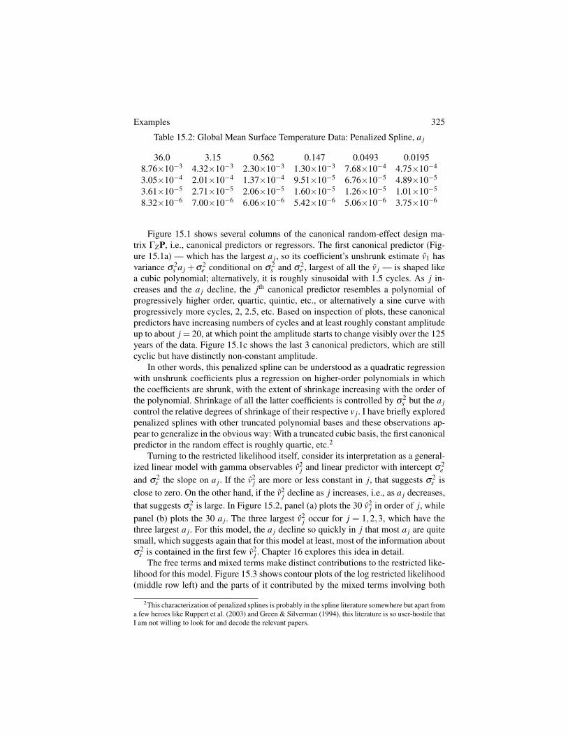
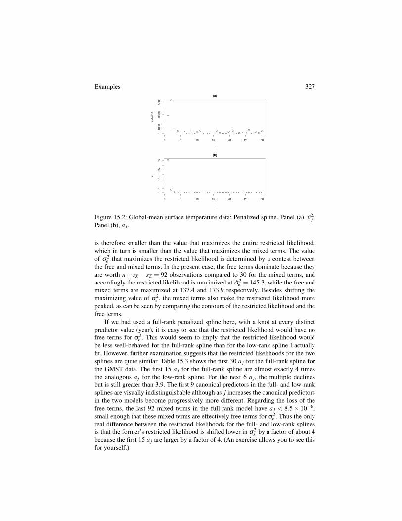
Table 15.2: Global Mean Surface Temperature Data: Penalized Spline, a j
36.0 3.15 0.562 0.147 0.0493 0.01958.76⇥10�3 4.32⇥10�3 2.30⇥10�3 1.30⇥10�3 7.68⇥10�4 4.75⇥10�4
3.05⇥10�4 2.01⇥10�4 1.37⇥10�4 9.51⇥10�5 6.76⇥10�5 4.89⇥10�5
3.61⇥10�5 2.71⇥10�5 2.06⇥10�5 1.60⇥10�5 1.26⇥10�5 1.01⇥10�5
8.32⇥10�6 7.00⇥10�6 6.06⇥10�6 5.42⇥10�6 5.06⇥10�6 3.75⇥10�6
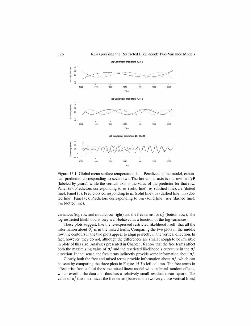
Figure 15.1 shows several columns of the canonical random-effect design ma-trix GZP, i.e., canonical predictors or regressors. The first canonical predictor (Fig-ure 15.1a) — which has the largest a j, so its coefficient’s unshrunk estimate v1 hasvariance s
2s a j +s
2e conditional on s
2s and s
2e , largest of all the v j — is shaped like
a cubic polynomial; alternatively, it is roughly sinusoidal with 1.5 cycles. As j in-creases and the a j decline, the jth canonical predictor resembles a polynomial ofprogressively higher order, quartic, quintic, etc., or alternatively a sine curve withprogressively more cycles, 2, 2.5, etc. Based on inspection of plots, these canonicalpredictors have increasing numbers of cycles and at least roughly constant amplitudeup to about j = 20, at which point the amplitude starts to change visibly over the 125years of the data. Figure 15.1c shows the last 3 canonical predictors, which are stillcyclic but have distinctly non-constant amplitude.
In other words, this penalized spline can be understood as a quadratic regressionwith unshrunk coefficients plus a regression on higher-order polynomials in whichthe coefficients are shrunk, with the extent of shrinkage increasing with the order ofthe polynomial. Shrinkage of all the latter coefficients is controlled by s
2s but the a j
control the relative degrees of shrinkage of their respective v j. I have briefly exploredpenalized splines with other truncated polynomial bases and these observations ap-pear to generalize in the obvious way: With a truncated cubic basis, the first canonicalpredictor in the random effect is roughly quartic, etc.2
Turning to the restricted likelihood itself, consider its interpretation as a general-ized linear model with gamma observables v2
j and linear predictor with intercept s
2e
and s
2s the slope on a j. If the v2
j are more or less constant in j, that suggests s
2s is
close to zero. On the other hand, if the v2j decline as j increases, i.e., as a j decreases,
that suggests s
2s is large. In Figure 15.2, panel (a) plots the 30 v2
j in order of j, whilepanel (b) plots the 30 a j. The three largest v2
j occur for j = 1,2,3, which have thethree largest a j. For this model, the a j decline so quickly in j that most a j are quitesmall, which suggests again that for this model at least, most of the information abouts
2s is contained in the first few v2
j . Chapter 16 explores this idea in detail.The free terms and mixed terms make distinct contributions to the restricted like-
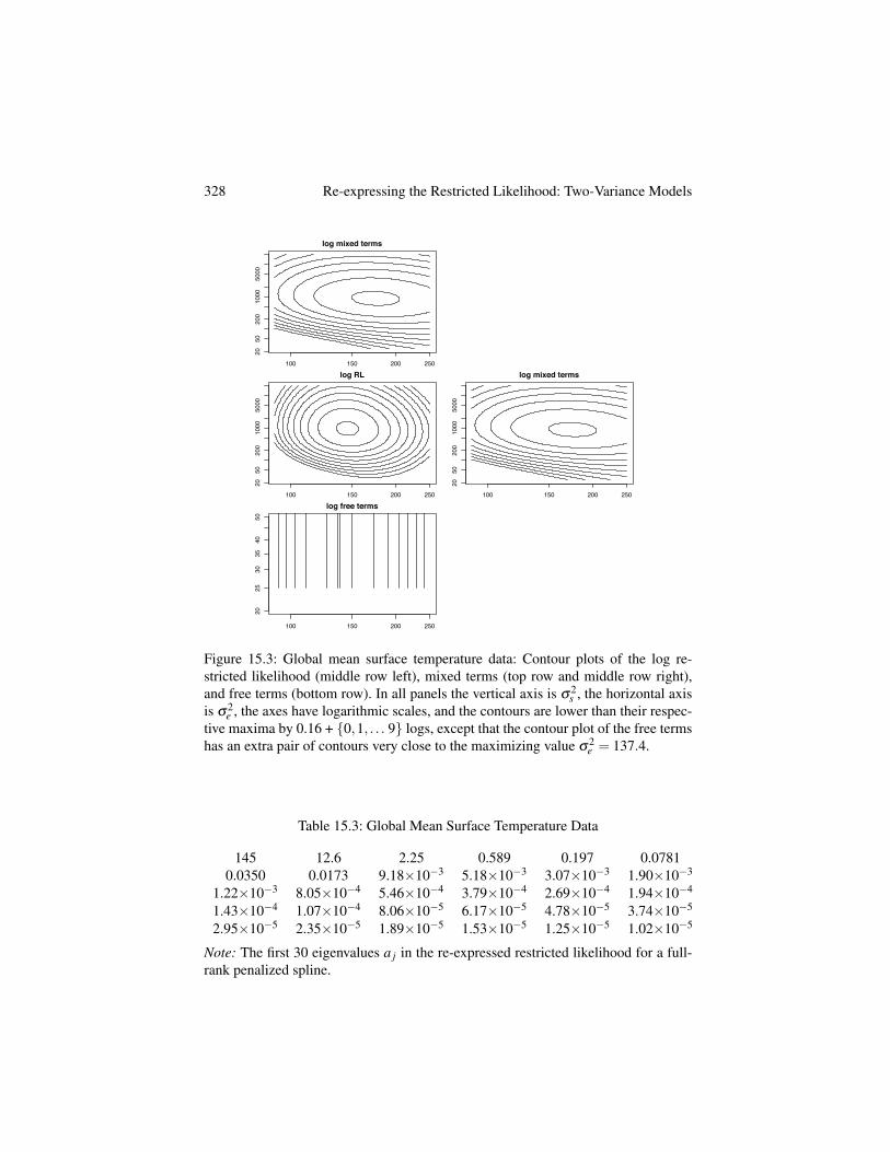
lihood for this model. Figure 15.3 shows contour plots of the log restricted likelihood(middle row left) and the parts of it contributed by the mixed terms involving both
2This characterization of penalized splines is probably in the spline literature somewhere but apart froma few heroes like Ruppert et al. (2003) and Green & Silverman (1994), this literature is so user-hostile thatI am not willing to look for and decode the relevant papers.
326 Re-expressing the Restricted Likelihood: Two-Variance Models
1880 1900 1920 1940 1960 1980 2000
−0.4
0.0
0.2
0.4
(a) Canonical predictors 1, 2, 3
Year
cano
nica
l pre
dict
or
1880 1900 1920 1940 1960 1980 2000
−0.4
0.0
0.2
0.4
(b) Canonical predictors 4, 5, 6
Year
cano
nica
l pre
dict
or
1880 1900 1920 1940 1960 1980 2000
−0.4
0.0
0.2
0.4
(c) Canonical predictors 28, 29, 30
Year
cano
nica
l pre
dict
or
Figure 15.1: Global mean surface temperature data: Penalized spline model, canon-ical predictors corresponding to several a j. The horizontal axis is the row in GZP(labeled by years), while the vertical axis is the value of the predictor for that row.Panel (a): Predictors corresponding to a1 (solid line), a2 (dashed line), a3 (dottedline). Panel (b): Predictors corresponding to a4 (solid line), a5 (dashed line), a6 (dot-ted line). Panel (c): Predictors corresponding to a28 (solid line), a29 (dashed line),a30 (dotted line).
variances (top row and middle row right) and the free terms for s
2e (bottom row). The
log restricted likelihood is very well-behaved as a function of the log variances.These plots suggest, like the re-expressed restricted likelihood itself, that all the
information about s
2s is in the mixed terms. Comparing the two plots in the middle
row, the contours in the two plots appear to align perfectly in the vertical direction. Infact, however, they do not, although the differences are small enough to be invisiblein plots of this size. Analyses presented in Chapter 16 show that the free terms affectboth the maximizing value of s
2s and the restricted likelihood’s curvature in the s
2s
direction. In that sense, the free terms indirectly provide some information about s
2s .
Clearly both the free and mixed terms provide information about s
2e , which can
be seen by comparing the three plots in Figure 15.3’s left column. The free terms ineffect arise from a fit of the same mixed linear model with unshrunk random effects,which overfits the data and thus has a relatively small residual mean square. Thevalue of s
2e that maximizes the free terms (between the two very close vertical lines)
Examples 327
0 5 10 15 20 25 30
01000
3000
5000
(a)
j
v−ha
t^2
0 5 10 15 20 25 30
05
1525
35(b)
j
a
Figure 15.2: Global-mean surface temperature data: Penalized spline. Panel (a), v2j ;
Panel (b), a j.
is therefore smaller than the value that maximizes the entire restricted likelihood,which in turn is smaller than the value that maximizes the mixed terms. The valueof s
2e that maximizes the restricted likelihood is determined by a contest between
the free and mixed terms. In the present case, the free terms dominate because theyare worth n� sX � sZ = 92 observations compared to 30 for the mixed terms, andaccordingly the restricted likelihood is maximized at s
2e = 145.3, while the free and
mixed terms are maximized at 137.4 and 173.9 respectively. Besides shifting themaximizing value of s
2e , the mixed terms also make the restricted likelihood more
peaked, as can be seen by comparing the contours of the restricted likelihood and thefree terms.
If we had used a full-rank penalized spline here, with a knot at every distinctpredictor value (year), it is easy to see that the restricted likelihood would have nofree terms for s
2e . This would seem to imply that the restricted likelihood would
be less well-behaved for the full-rank spline than for the low-rank spline I actuallyfit. However, further examination suggests that the restricted likelihoods for the twosplines are quite similar. Table 15.3 shows the first 30 a j for the full-rank spline forthe GMST data. The first 15 a j for the full-rank spline are almost exactly 4 timesthe analogous a j for the low-rank spline. For the next 6 a j, the multiple declinesbut is still greater than 3.9. The first 9 canonical predictors in the full- and low-ranksplines are visually indistinguishable although as j increases the canonical predictorsin the two models become progressively more different. Regarding the loss of thefree terms, the last 92 mixed terms in the full-rank model have a j < 8.5⇥ 10�6,small enough that these mixed terms are effectively free terms for s
2e . Thus the only
real difference between the restricted likelihoods for the full- and low-rank splinesis that the former’s restricted likelihood is shifted lower in s
2s by a factor of about 4
because the first 15 a j are larger by a factor of 4. (An exercise allows you to see thisfor yourself.)
328 Re-expressing the Restricted Likelihood: Two-Variance Models
log mixed terms
100 150 200 250
2050
200
1000
5000
log RL
100 150 200 250
2050
200
1000
5000
log mixed terms
100 150 200 250
2050
200
1000
5000
log free terms
100 150 200 250
2025
3035
4050
Figure 15.3: Global mean surface temperature data: Contour plots of the log re-stricted likelihood (middle row left), mixed terms (top row and middle row right),and free terms (bottom row). In all panels the vertical axis is s
2s , the horizontal axis
is s
2e , the axes have logarithmic scales, and the contours are lower than their respec-
tive maxima by 0.16 + {0,1, . . . 9} logs, except that the contour plot of the free termshas an extra pair of contours very close to the maximizing value s
2e = 137.4.
Table 15.3: Global Mean Surface Temperature Data
145 12.6 2.25 0.589 0.197 0.07810.0350 0.0173 9.18⇥10�3 5.18⇥10�3 3.07⇥10�3 1.90⇥10�3
1.22⇥10�3 8.05⇥10�4 5.46⇥10�4 3.79⇥10�4 2.69⇥10�4 1.94⇥10�4
1.43⇥10�4 1.07⇥10�4 8.06⇥10�5 6.17⇥10�5 4.78⇥10�5 3.74⇥10�5
2.95⇥10�5 2.35⇥10�5 1.89⇥10�5 1.53⇥10�5 1.25⇥10�5 1.02⇥10�5
Note: The first 30 eigenvalues a j in the re-expressed restricted likelihood for a full-rank penalized spline.

Examples 329
15.2.3 ICAR Model; Spatial Confounding Revisited
First we consider Section 14.1’s simple ICAR model for the attachment-loss data,contrasting it with the penalized spline model just discussed. Then we consider theICAR model with one fixed-effect predictor that was used to explore spatial con-founding in Sections 9.1.1 and 10.1. This allows us to say more about some questionsthat were left open at the end of Section 10.1.
15.2.3.1 Attachment-Loss Data: Simple ICAR Model
Section 14.1 fit a simple ICAR model, with no explicit fixed-effect predictors, tothe attachment-loss data shown in Figure 14.1. For this dataset, the spatial map hasI = 2 islands, one each for the maxillary (upper) and mandibular (lower) arches,so the ICAR model has p = sX = 2 implicit fixed effects, intercepts or means forthe two islands. This person had n = 168 measurement sites, so the ICAR model’srandom effects have q = sZ = 166. The neighbor pairings of measurement sites areas shown in Figure 14.2, although the present analysis does not distinguish types ofneighbor pairs. The data are sorted as in Figure 14.1: Maxilla then mandible; withinarch, lingual (tongue side) then buccal (cheek side); and within arch and side, fromleft to right as in Figure 14.1. Before reading further, it may be helpful to reviewSection 5.2.2.
In the mixed-linear-model formulation of the ICAR model given in Section 5.2.2,the random effects q 1 have covariance matrix s
2s D�1
1 , where D1 is a diagonal matrixcontaining the positive eigenvalues of Q, the matrix that encodes the ICAR’s neigh-bor pairings (and which is proportional to the prior precision of the ICAR randomeffect). This covariance matrix, s
2s D�1
1 , is not proportional to the identity so beforewe begin, the ICAR model’s random effects V1q 1, as written in equation (5.14), mustbe re-parameterized. Using the notation of Section 5.2.2, for the present purpose thefixed effect design matrix is X = V2, of which the two columns are indicators for themaxillary and mandibular islands; the random effect design matrix is Z = V1D�0.5
1 ,where V1’s columns are the eigenvectors of Q that have positive eigenvalues; and therandom effects are u = D0.5
1 q1 with covariance matrix G = s
2s In�2.
Define Wm as an m⇥m matrix with 1’s down the diagonal from upper right tolower left and 0’s elsewhere; post-multiplying a matrix by Wm reverses the order ofits columns, pre-multiplying by Wm reverses the order of its rows. If we follow thesteps in re-expressing the restricted likelihood, GZ = V1, A = WsZ D�1
1 WsZ , and P =WsZ so the canonical observations are v= (V1WsZ )
0y. These v are the same contrastsin the data that were examined in Section 5.2.2, but their order has been reversed:V1’s columns were sorted in decreasing order of the precisions of the random effectsq 1, while the canonical predictors are sorted in decreasing order of the variances ofthe canonical random effects v.3
Consider the a j in the re-expressed restricted likelihood, summarized in Ta-ble 15.4. Because this subject has no missing teeth, the maxillary and mandibular
3I apologize for this notational kluge. ICARs were largely developed by Bayesians, who like preci-sions, while mixed-linear-model theory was largely developed by non-Bayesians, who prefer variances.Sometimes the translation is awkward.

330 Re-expressing the Restricted Likelihood: Two-Variance Models
Table 15.4: Simple ICAR Model for the Attachment-Loss Data: Summary of the166 a j
Number ofa j Multiplicity Distinct a j
149.0 2 137.33 2 116.64 2 1
9.40 to 1 2 110.843 4 10.695 24 1
0.672 to 0.333 2 140.288 4 10.200 24 1
0.1996 to 0.1872 2 70.1872 4 1
0.1858 to 0.1800 2 60.1798 24 1
arches have identical spatial structures so the multiplicity of each a j is an even num-ber split equally between the two arches. Some a j have multiplicity 24, 12 per arch,referring to the 12 interior teeth in an arch; others have multiplicity 4, 2 per arch,referring to the 2 “edge” teeth in each arch, labeled as tooth number 7 in Figure 14.1.
Compared to the a j for the penalized spline, the ICAR’s a j decrease much moreslowly in j. For the penalized spline, a1/a6 = 1,841; for the ICAR, a1/a6 = 9.0. (Ar-guably a1/a12 = 35.2 is a more fair comparison because the ICAR’s spatial structureis identical in the two arches, but my point stands.) For the spline, a1/a15 = 263,083;for the ICAR, a1/a15 = 61.4 (a1/a30 = 177). The ratio of largest to smallest a j is9,593,165 for the spline and 829 for the ICAR, and the ICAR has 166 a j comparedto the spline’s 30. This means that shrinkage of the canonical random effects v j ismuch less differentiated for the ICAR than for the spline. This appears to be true ofICAR models generally and as we will see in Chapter 16, this fact helps explain whythe penalized spline and ICAR models smooth the global mean surface temperaturedata so differently (Section 14.3).
The ICAR’s canonical predictors, on the other hand, are fairly similar to thespline’s canonical predictors. Figure 15.4 shows several canonical predictors. Thetwo arches have identical sets of 83 canonical predictors and for each arch, the firstfew canonical predictors are identical on the buccal and lingual sides of the arch.Thus, Figure 15.4 shows the values of the first few canonical predictors for one sideof one arch. The ICAR’s first 8 canonical predictors, i.e., the first 4 in each arch,strongly resemble sine curves. The first canonical predictor in each arch (Panel (a))is close to a half-cycle of a sine curve. The second canonical predictor in each arch(Panel (b)) resembles a full cycle of a sine curve; each of the next two canonical pre-dictors (Panels (c) and (d)) adds a half-cycle. Each canonical predictor deviates from
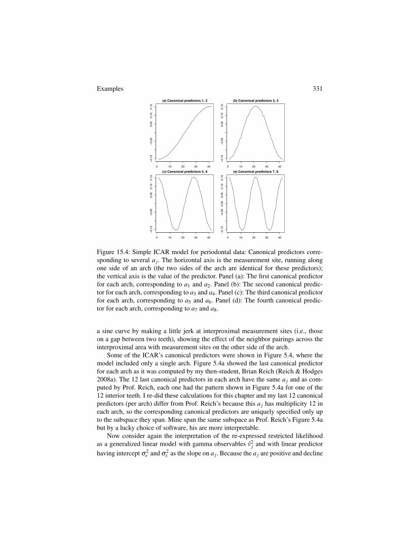
Examples 331
0 10 20 30 40
−0.1
5−0
.05
0.05
0.10
0.15
(a) Canonical predictors 1, 2
site
0 10 20 30 40
−0.1
5−0
.05
0.05
0.10
0.15
(b) Canonical predictors 3, 4
site
0 10 20 30 40
−0.1
5−0
.05
0.05
0.10
0.15
(c) Canonical predictors 5, 6
0 10 20 30 40
−0.1
5−0
.05
0.00
0.05
0.10
0.15
(e) Canonical predictors 7, 8
Figure 15.4: Simple ICAR model for periodontal data: Canonical predictors corre-sponding to several a j. The horizontal axis is the measurement site, running alongone side of an arch (the two sides of the arch are identical for these predictors);the vertical axis is the value of the predictor. Panel (a): The first canonical predictorfor each arch, corresponding to a1 and a2. Panel (b): The second canonical predic-tor for each arch, corresponding to a3 and a4. Panel (c): The third canonical predictorfor each arch, corresponding to a5 and a6. Panel (d): The fourth canonical predic-tor for each arch, corresponding to a7 and a8.
a sine curve by making a little jerk at interproximal measurement sites (i.e., thoseon a gap between two teeth), showing the effect of the neighbor pairings across theinterproximal area with measurement sites on the other side of the arch.
Some of the ICAR’s canonical predictors were shown in Figure 5.4, where themodel included only a single arch. Figure 5.4a showed the last canonical predictorfor each arch as it was computed by my then-student, Brian Reich (Reich & Hodges2008a). The 12 last canonical predictors in each arch have the same a j and as com-puted by Prof. Reich, each one had the pattern shown in Figure 5.4a for one of the12 interior teeth. I re-did these calculations for this chapter and my last 12 canonicalpredictors (per arch) differ from Prof. Reich’s because this a j has multiplicity 12 ineach arch, so the corresponding canonical predictors are uniquely specified only upto the subspace they span. Mine span the same subspace as Prof. Reich’s Figure 5.4abut by a lucky choice of software, his are more interpretable.
Now consider again the interpretation of the re-expressed restricted likelihoodas a generalized linear model with gamma observables v2
j and with linear predictorhaving intercept s
2e and s
2s as the slope on a j. Because the a j are positive and decline
332 Re-expressing the Restricted Likelihood: Two-Variance Models
0 50 100 150
010
2030
40
(a)
j
v−ha
t^2
0 50 100 150
02
46
810
(b)
j
v−ha
t^2
0 50 100 150
050
100
150
(c)
j
a
Figure 15.5: ICAR fit to the attachment loss data: Panel (a), v2j with full vertical scale;
Panel (b), v2j with vertical scale restricted to 0 to 10; Panel (c), a j.
as j increases, if this model fits the v2j should generally decline as j increases. For the
attachment-loss data, Figure 15.5 shows the v2j (Panels (a) and (b), identical except
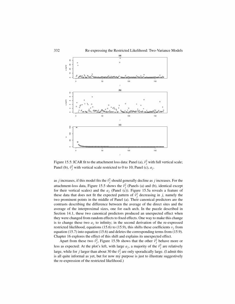
for their vertical scales) and the a j (Panel (c)). Figure 15.5a reveals a feature ofthese data that does not fit the expected pattern of v2
j decreasing in j, namely thetwo prominent points in the middle of Panel (a). Their canonical predictors are thecontrasts describing the difference between the average of the direct sites and theaverage of the interproximal sizes, one for each arch. In the puzzle described inSection 14.1, these two canonical predictors produced an unexpected effect whenthey were changed from random effects to fixed effects. One way to make this changeis to change these two a j to infinity; in the second derivation of the re-expressedrestricted likelihood, equations (15.6) to (15.9), this shifts these coefficients v j fromequation (15.7) into equation (15.6) and deletes the corresponding terms from (15.9).Chapter 16 explores the effect of this shift and explains its unexpected effect.
Apart from these two v2j , Figure 15.5b shows that the other v2
j behave more orless as expected: At the plot’s left, with large a j, a majority of the v2
j are relativelylarge, while for j larger than about 30 the v2
j are only sporadically large. (I admit thisis all quite informal as yet, but for now my purpose is just to illustrate suggestivelythe re-expression of the restricted likelihood.)
Examples 333
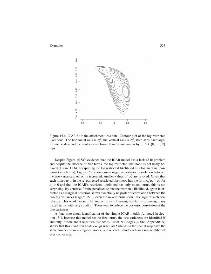
0.2 0.5 1.0 2.0 5.0
0.01
0.02
0.05
0.10
0.20
0.50
1.00
2.00
5.00
Figure 15.6: ICAR fit to the attachment loss data: Contour plot of the log restrictedlikelihood. The horizontal axis is s
2e , the vertical axis is s
2s , both axes have loga-
rithmic scales, and the contours are lower than the maximum by 0.16 + {0, . . . , 9}logs.
Despite Figure 15.5a’s evidence that the ICAR model has a lack-of-fit problemand despite the absence of free terms, the log restricted likelihood is not badly be-haved (Figure 15.6). Interpreting the log restricted likelihood as a log marginal pos-terior (which it is), Figure 15.6 shows some negative posterior correlation betweenthe two variances: As s
2s is increased, smaller values of s
2e are favored. Given that
each mixed term in the re-expressed restricted likelihood has the form s
2s a j +s
2e for
a j > 0 and that the ICAR’s restricted likelihood has only mixed terms, this is notsurprising. By contrast, for the penalized spline the restricted likelihood, again inter-preted as a marginal posterior, shows essentially no posterior correlation between thetwo log variances (Figure 15.3); even the mixed terms show little sign of such cor-relation. This would seem to be another effect of having free terms or having manymixed terms with very small a j: These tend to reduce the posterior correlation of thetwo variances.
A final note about identification of the simple ICAR model: As noted in Sec-tion 15.1, because this model has no free terms, the two variances are identified ifand only if there are at least two distinct a j. Reich & Hodges (2008a, Appendix A)shows that this condition holds except when all I islands in the spatial map have thesame number of areas (regions, nodes) and on each island, each area is a neighbor ofevery other area.
334 Re-expressing the Restricted Likelihood: Two-Variance Models
15.2.3.2 Spatial Confounding: ICAR with Predictors
The re-expressed restricted likelihood allows us to examine some aspects of the spa-tial confounding problem that Section 10.1.5 described as underdeveloped. I presentresults for a one-dimensional fixed-effect predictor F as in Section 10.1, but exten-sion to higher-dimensional F is straightforward. As before, F is centered and scaledso F0F = n�1.
Following the notation in Chapters 5 and 10, the model (before re-expression) isy = Fb + InS+e , where S is an n-dimensional ICAR random effect with smoothingvariance s
2s and adjacency matrix Q, i.e., with precision matrix Q/s
2s . For simplic-
ity, assume the spatial map is connected, with I = 1 island, so Q’s zero eigenvaluehas multiplicity 1. (This also generalizes in the obvious way.) As before, Q has spec-tral decomposition Q = VDV0, where V is an orthogonal matrix that partitions as(V1| 1p
n 1n), where V1 is n⇥ (n�1), and D is diagonal with nth diagonal entry zero;its upper left (n�1)⇥ (n�1) partition D1 is a diagonal matrix with positive entriesd1 � . . .� dn�1 > 0.
Then as in equation (5.15), the model can be rewritten as
y = 1nb0 +Fb +V1q 1 + e (15.12)
where the now-explicit intercept b0 has absorbed the factor 1/p
n and q 1 ⇠N(0,s2
s D�11 ), where s
2s D�1
1 is a covariance matrix. To follow the derivation of there-expressed restricted likelihood, the random effect must be re-parameterized so itscovariance is proportional to the identity, so for the present purpose, X = (1n|F) andZ = V1D�0.5
1 .Following the derivation of the re-expressed restricted likelihood, GX =
( 1pn 1n| 1p
n�1 F). As noted, GZ is not unique but the restricted likelihood is invari-ant to the choice of GZ . Recall, however, that GZ is defined so that (GX |GZ) is abasis for the column space of (X|Z) and G0
X GZ = 0. MZZ = G0ZZ = G0
ZV1D�0.51 , so
MZZM0ZZ = G0
ZV1D�11 V0
1GZ . In the re-expression, the final key items are obtainedfrom the spectral decomposition MZZM0
ZZ =PAP0. The canonical predictors are GZPand the canonical observations are v = P0G0
Zy. Unfortunately, A, GZP, and v do nothave simple forms in general. I consider special cases below, some of which do yieldsimple forms.
The rest of this subsection considers two questions about the restricted likeli-hood. First, given the spatial map, which implies V1 and D1, how does the fixedeffect F affect the restricted likelihood and thus, through s
2s and s
2e , the amount
of spatial smoothing and the potential severity of spatial confounding? Second, it iswidely believed that adding the spatial random effect S will adjust the estimate ofb for an omitted fixed-effect predictor H. Section 10.1.4.1 debunked this belief us-ing derivations that assumed the data were in fact generated by Model H in whichy= 1nb0+Fb +Hg+e . Those derivations treated the variances s
2s and s
2e as known
but now we can, to some extent, examine the information about them in the restrictedlikelihood (and thus in the posterior distribution arising from a flat prior on (b0,b ).Thus the second question about the restricted likelihood is: If the data were in fact
Examples 335
generated by Model H, how does the specific H affect the restricted likelihood andthus the amount of spatial smoothing and the potential for spatial confounding?
So: How does the fixed effect F affect the restricted likelihood? I can’t answerthis in general, but I present three illuminating special cases. In the first, F is exactlyproportional to the kth column of V1. In this case, GZ = V(�k)
1 , where this notationindicates V1 with its kth column deleted. Then MZZM0
ZZ = (D(�k)1 )�1, where D(�k)
1 isD1 with its kth row and column deleted, which implies P = Wn�2 (Wm was definedabove as the m⇥m matrix with 1’s down the diagonal from upper right to lower leftand 0’s elsewhere) and A = Wn�2(D(�k)
1 )�1Wn�2. The canonical predictors are thecolumns of V(�k)
1 Wn�2 and the canonical observations are v = (V(�k)1 Wn�2)0y. The
information about s
2s comes from contrasts in the data corresponding to the columns
of V1, the eigenvectors of the adjacency matrix Q, excluding the contrast proportionalto F, which does not contribute to the restricted likelihood but rather informs onlyabout the fixed effects.
This special case presents two distinct possibilities. If in fact the data were gen-erated from the true model y = 1nb0 +Fb + e , so all variation in y apart from F isiid, then in truth var(v j|s2
s ,s2e ) = s
2e . Considering the re-expressed restricted like-
lihood as a gamma regression with “data” v2j and linear predictor s
2s a j + s
2e , s
2s
will generally be estimated as being close to zero, so S will be shrunk close to zero,and spatial confounding cannot occur. This partially contradicts one of the hypothe-ses stated in Section 10.1.5. On the other hand, if the true data-generating model isy = 1nb0 +Fb +V(�k)
1 g + e for some non-trivial g , then s
2s may have a large es-
timate. I am not sure whether spatial confounding can occur in this case. The keyequations here are (10.3) and (10.4), which show the change in the estimate of b
from adding the spatial random effect; the complication arises from the effect of rDin equation (10.4). Exploring this question is an exercise; I don’t think it will be toohard but my deadline looms.
In transforming from the original model, equation (15.12), to the re-parameterized model that gives the re-expressed restricted likelihood, the randomeffects lose one dimension corresponding to the column space of the fixed effect F.In the very simple special case just discussed, where F is exactly proportional to thekth column of V1, this transition is simple: GZ is simply V1 without its kth column.But what happens when F is not proportional to any column in V1?
To explore this, our second special case is the Slovenian stomach-cancer dataconsidered in Chapters 5, 9, and 10. Here, n = 194 and F is the centered and scaledindicator of socioeconomic status. It has correlation 0.72 with V1,193, the randomeffect design-matrix column for which the random effect, q1,193, has the largest vari-ance d�1
193s
2s among all the random effects. Because the squared correlations between
F and the columns of V1 must add to 1 (see Section 10.1), F cannot have a very largecorrelation with any other column of V1; the 2nd and 3rd largest correlations are 0.23with V1,34 and -0.13 with V1,173. In deriving GZ and the canonical predictors GZP,we remove from V1’s columns the parts that lie in the column space of F and omita column to obtain the 192 canonical predictors. Given the high correlation between
336 Re-expressing the Restricted Likelihood: Two-Variance Models
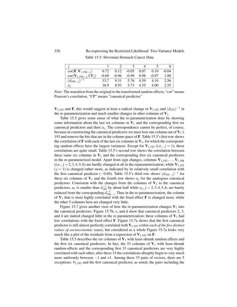
Table 15.5: Slovenian Stomach-Cancer Data
j 1 2 3 4 5 6cor(F,V1,194� j) 0.72 0.12 -0.05 0.07 0.10 -0.04cor(V1,194� j,CP j) -0.69 -0.96 -0.99 0.98 -0.97 1.00(d194� j)�1 33.7 9.31 5.76 4.59 4.10 2.56a j 16.9 8.93 5.73 4.55 4.00 2.55
Note: The transition from the original to the transformed random effects; “cor” meansPearson’s correlation, “CP” means ”canonical predictor.”
V1,193 and F, this would suggest at least a radical change in V1,193 and (d193)�1 inthe re-parameterization and much smaller changes in other columns of V1.
Table 15.5 gives some sense of what the re-parameterization does by showingsome information about the last six columns in V1 and the corresponding first sixcanonical predictors and their a j. The correspondence cannot be perfect, of course,because in constructing the canonical predictors we must lose one column out of V1’s193 and remove the bits that are in the column space of F. Table 15.5’s first row showsthe correlation of F with each of the last six columns in V1, for which the correspond-ing random effects have the largest variances. Except for V1,193 (i.e., j = 1), thesecorrelations are quite small. Table 15.5’s second row shows the correlation betweenthese same six columns in V1 and the corresponding first six canonical predictorsin the re-parameterized model. Apart from sign changes, columns V1,192, . . . ,V1,188(i.e., j = 2,3,4,5,6) are hardly changed at all in the reparameterization, while V1,193( j = 1) is changed rather more, as indicated by its relatively small correlation withthe first canonical predictor (�0.69). Table 15.5’s third row shows (d194� j)�1 forthese six columns of V1 and the fourth row shows a j for the analogous canonicalpredictors. Consistent with the changes from the columns of V1 to the canonicalpredictors, a1 is smaller than d�1
193 by about half while a j, j = 2,3,4,5,6, are barelyreduced from the corresponding d�1
194� j. Thus in the re-parameterization, the columnof V1 that is most highly correlated with the fixed effect F is changed most, whilethe other 5 columns here are changed very little.
Figure 15.7 gives another view of how the re-parameterization changes V1 intothe canonical predictors. Figure 15.7b, c, and d show that canonical predictors 2, 3,and 4 are indeed changed little in the re-parameterization; these columns of V1 hadlow correlations with the fixed effect F. Figure 15.7a shows that the first canonicalpredictor is still almost perfectly correlated with V1,193 within each of the five distinctvalues of socioeconomic status, but considered as a whole Figure 15.7a looks verymuch like a plot of the residuals from a regression of V1,193 on F.
Table 15.5 describes the six columns of V1 with least-shrunk random effects andthe first six canonical predictors. In fact, the 33 columns of V1 with least-shrunkrandom-effects and the corresponding first 33 canonical predictors are very highlycorrelated with each other; after these 33 the correlations abruptly begin to vary muchmore uniformly between �1 and +1. Among these 33 pairs of vectors, there are 5exceptions: V1,193 and the first canonical predictor, as noted; the pairs including the
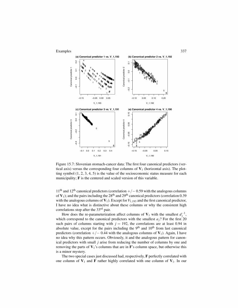
Examples 337
−0.15 −0.05 0.00 0.05
−0.1
0.0
0.1
0.2
(a) Canonical predictor 1 vs. V_1,193
V_1,193
Can
onic
al p
redi
ctor
111
22
111
2
1
1
2
2
3
4
21
2
1
33
32
2
1
2
53
1
3
3
3
1
3
4
3
23
22
2
2
2
1
53
121
4
1
5
244
2
3
24
3
4
4
3
3 4
4
4
5
5
1
3555
2 3 5
2
53
25
3
241
35
5
2
25 5
5
1
55
3
4
3
452 4
244
5
4
55
32
3
3
555
22
4
55 55
5
3
554
34
5
2
555
2
455
55
5
2
4 5
3
4
44 55554
55
4555
3
55
5
3
45
43 4
5
3
5
4
5 5
3
45
344
2
4
34
54
5
2
55
2
−0.10 0.00 0.10 0.20
−0.2
−0.1
0.0
0.1
(b) Canonical predictor 2 vs. V_1,192
V_1,192
Can
onic
al p
redi
ctor
2
11 22111
21
1
2
2
34
2
1
21
33
32 21
2
5
3
1
3
33
1 3
43
2
322
2
2
2
1
53
1
2
1
4
15
2
44
2
3
2
43 4
4
3
3
44 45
51
3
555
2
35
2 5
3
2
5
324
1
3
5
522 5
5
5
1
5
5
3
4
34
5
242
4
4 5
4
55
323
3
5
5
522
455
5
5
5
35
5
4
34
5255
524
5
5
5
5
52 4
5
3 4
44
55
55
4554
5
55
3
5
5
5
3
4
54
3
45
3
5
45
5
3
4
5
3
442
43
45
4
5
2
55
2
−0.1 0.0 0.1 0.2 0.3 0.4
−0.4
−0.2
0.0
0.1
(c) Canonical predictor 3 vs. V_1,191
V_1,191
Can
onic
al p
redi
ctor
3
112211121
1
2
2
34
2
1
21
33 32
21
2
531
3
331343
23
22
222 15
3121
415
244
2
3
24
344
3
344
4
5
5 1
3
555
23
525
32
53
2
4
1
3
55
22
55
51
55
34
345
2
42
445
4
553
23
3555
22
45555
53554
3452
5552
455555 24534
4455554554 555355534543
453
545
5
34
5
3
44243
4
5
4
5
2
55
2
−0.15 −0.05 0.05 0.15
−0.1
5−0
.05
0.05
0.15
(e) Canonical predictor 4 vs. V_1,190
V_1,190
Can
onic
al p
redi
ctor
4
11
2
211121
1
2
2
34
2
1
21
3
332
21
25
31
3
3
3
1
343
23
22
2
221
5
3
121
41
5
2442
3
2
4
34
4
3
34
4
4
5
5
1
3
5
55
23
5
2
53
25
3
2
4
1
3
5
5
2
2
5
5
5
15
53
43
4
52
42
4
4 54
55
32
3
35
5
52
2455
5
5
5
35
5
4
3
4
5255
52 4
5
5
5
5
52
4
53
4
44
55
55
4
554
5
55
3
5
5
5
3
4
5
43
45
3
5
4
5
5
3
4
5
3
44
2
43
45
4 5
2
55
2
Figure 15.7: Slovenian stomach-cancer data: The first four canonical predictors (ver-tical axis) versus the corresponding four columns of V1 (horizontal axis). The plot-ting symbol (1, 2, 3, 4, 5) is the value of the socioeconomic status measure for eachmunicipality; F is the centered and scaled version of this variable.
11th and 12th canonical predictors (correlation +/� 0.59 with the analogous columnsof V1); and the pairs including the 28th and 29th canonical predictors (correlation 0.39with the analogous columns of V1). Except for V1,193 and the first canonical predictor,I have no idea what is distinctive about these columns or why the consistent highcorrelations stop after the 33rd pair.
How does the re-parameterization affect columns of V1 with the smallest d�1j ,
which correspond to the canonical predictors with the smallest a j? For the first 20such pairs of columns starting with j = 192, the correlations are at least 0.94 inabsolute value, except for the pairs including the 9th and 10th from last canonicalpredictors (correlation +/� 0.44 with the analogous columns of V1). Again, I haveno idea why this pattern occurs. Obviously, it and the analogous pattern for canon-ical predictors with small j arise from reducing the number of columns by one andremoving the parts of V1’s columns that are in F’s column space, but otherwise thisis a minor mystery.
The two special cases just discussed had, respectively, F perfectly correlated withone column of V1 and F rather highly correlated with one column of V1. In our
338 Re-expressing the Restricted Likelihood: Two-Variance Models
third special case, F = V11193, which has the same correlation (0.023) with all 193columns of V1. We might expect all the columns of V1 to be affected about equallyin the re-parameterization and they are. Reflecting this equal treatment and the needto lose one column in the re-parameterization, V1,194� j and canonical predictor jhave correlations with absolute value at least 0.94 for j = 1, . . . ,27; as j increasesfurther, these correlations vary in a progressively wider band, though up to j = 100the smallest absolute correlation is 0.52. Similarly, the a j are reduced very little com-pared to d�1
194� j: The ratio lies in the interval 0.982 to 1 for j = 1, . . . ,183 and overallthe smallest ratio is 0.938.
Now for the second question about the restricted likelihood in the spatial-confounding case: If the data were in fact generated by Model H, in which y =1nb0 +Fb +Hg + e , how does the specific true H affect the restricted likelihood?Under Model H,
v = P0G0Zy
= P0G0Z(1nb0 +Fb +Hg + e)
= P0G0ZHg +P0G0
Ze. (15.13)
Because P0G0Z has orthonormal rows, P0G0
Ze ⇠ N(0,s2e IsZ ), so conditional on s
2e , v
is normal with covariance s
2e IsZ and mean P0G0
ZHg . P0G0ZHg is the vector of coeffi-
cient estimates in a regression of Hg on the canonical predictors GZP. Thus, v j willtend to be large if H is highly correlated with canonical predictor j. Recalling thatthe re-expressed restricted likelihood is a gamma regression with “data” v2
j and lin-ear predictor s
2s a j +s
2e , it is clear that for Hg of a given magnitude, the restricted
likelihood will depend strongly on which canonical predictors j happen to be highlycorrelated with H.
Because the a j decline as j increases, if s
2s is large, the s
2s a j +s
2e decline as j
increases, while if s
2s is small or zero, the s
2s a j +s
2e are more or less constant in
j. Thus, if H is highly correlated with canonical predictor 1, v21 will be large, the
restricted likelihood will tend to indicate a large s
2s , and the random effect will not
be shrunk much. This creates the possibility of spatial confounding as well as thepossibility that the spatial random effect will adjust F’s coefficient b for the omittedpredictor H. On the other hand, if H is highly correlated with canonical predictor jfor large j, then that v2
j will be large and other v2j will be small and the restricted
likelihood will tend to indicate a small s
2s . In this case, the random effect will be
shrunk close to zero so spatial confounding cannot occur but the spatial randomeffect also cannot adjust F’s coefficient b for the omitted predictor H.
The actual results for a given H will depend not just on how H projects on thevarious canonical predictors but also on g and s
2e . An exercise explores the effect of
H in detail for the Slovenian stomach-cancer dataset.
15.2.4 Dynamic Linear Model with One Quasi-Cyclic Component
For the present purpose I consider a simplified version of the dynamic linear model(DLM) used for Michael Lavine’s dataset on localizing epileptic activity in the brain,discussed in Chapters 6, 9, and 12. Specifically, consider a data series with 650 time
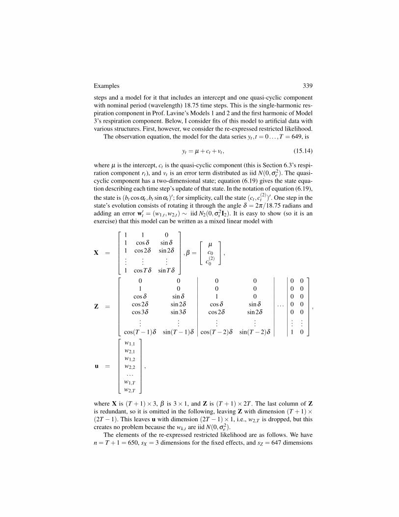
Examples 339
steps and a model for it that includes an intercept and one quasi-cyclic componentwith nominal period (wavelength) 18.75 time steps. This is the single-harmonic res-piration component in Prof. Lavine’s Models 1 and 2 and the first harmonic of Model3’s respiration component. Below, I consider fits of this model to artificial data withvarious structures. First, however, we consider the re-expressed restricted likelihood.
The observation equation, the model for the data series yt , t = 0 . . . ,T = 649, is
yt = µ + ct + vt , (15.14)
where µ is the intercept, ct is the quasi-cyclic component (this is Section 6.3’s respi-ration component rt ), and vt is an error term distributed as iid N(0,s2
e ). The quasi-cyclic component has a two-dimensional state; equation (6.19) gives the state equa-tion describing each time step’s update of that state. In the notation of equation (6.19),the state is (bt cosat ,bt sinat)0; for simplicity, call the state (ct ,c
(2)t )0. One step in the
state’s evolution consists of rotating it through the angle d = 2p/18.75 radians andadding an error w0
t = (w1,t ,w2,t) ⇠ iid N2(0,s2s I2). It is easy to show (so it is an
exercise) that this model can be written as a mixed linear model with
X =
2
666664
1 1 01 cosd sind
1 cos2d sin2d
......
...1 cosT d sinT d
3
777775,b =
2
4µ
c0
c(2)0
3
5 ,
Z =
2
6666666664
0 0 0 0 0 01 0 0 0 0 0
cosd sind 1 0 0 0cos2d sin2d cosd sind . . . 0 0cos3d sin3d cos2d sin2d 0 0
......
......
......
cos(T �1)d sin(T �1)d cos(T �2)d sin(T �2)d 1 0
3
7777777775
,
u =
2
666666664
w1,1w2,1w1,2w2,2. . .
w1,Tw2,T
3
777777775
,
where X is (T + 1)⇥ 3, b is 3⇥ 1, and Z is (T + 1)⇥ 2T . The last column of Zis redundant, so it is omitted in the following, leaving Z with dimension (T + 1)⇥(2T � 1). This leaves u with dimension (2T � 1)⇥ 1, i.e., w2,T is dropped, but thiscreates no problem because the wk,t are iid N(0,s2
e ).The elements of the re-expressed restricted likelihood are as follows. We have
n = T +1 = 650, sX = 3 dimensions for the fixed effects, and sZ = 647 dimensions
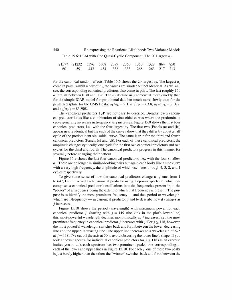
340 Re-expressing the Restricted Likelihood: Two-Variance Models
Table 15.6: DLM with One Quasi-Cyclic Component: The 20 Largest a j
21577 21232 5396 5308 2399 2360 1350 1328 864 850601 591 442 434 338 333 268 263 217 213
for the canonical random effects. Table 15.6 shows the 20 largest a j. The largest a jcome in pairs; within a pair of a j, the values are similar but not identical. As we willsee, the corresponding canonical predictors also come in pairs. The last roughly 150a j are all between 0.30 and 0.26. The a j decline in j somewhat more quickly thanfor the simple ICAR model for periodontal data but much more slowly than for thepenalized spline for the GMST data: a1/a6 = 9.1, a1/a15 = 63.8, a1/a166 = 8,072,and a1/a647 = 83,908.
The canonical predictors GZP are not easy to describe. Broadly, each canoni-cal predictor looks like a combination of sinusoidal curves where the predominantcurve generally increases in frequency as j increases. Figure 15.8 shows the first fourcanonical predictors, i.e., with the four largest a j. The first two (Panels (a) and (b))appear nearly identical but the ends of the curves show that they differ by about a halfcycle of the predominant sinusoidal curve. The same is true for the third and fourthcanonical predictors (Panels (c) and (d)). For each of these canonical predictors, theamplitude changes cyclically, one cycle for the first two canonical predictors and twocycles for the third and fourth. The canonical predictors progress in this manner forseveral j before changing their pattern.
Figure 15.9 shows the last four canonical predictors, i.e., with the four smallesta j. These are no longer in similar-looking pairs but again each looks like a sine curvewith a very high frequency, the amplitude of which oscillates through 4, 3, 2, and 1cycles respectively.
To give some sense of how the canonical predictors change as j runs from 1to 647, I summarized each canonical predictor using its power spectrum, which de-composes a canonical predictor’s oscillations into the frequencies present in it, the“power” of a frequency being the extent to which that frequency is present. The pur-pose is to identify the most prominent frequency — and thus period or wavelength,which are 1/frequency — in canonical predictor j and to describe how it changes asj increases.
Figure 15.10 shows the period (wavelength) with maximum power for eachcanonical predictor j. Starting with j = 119 (the kink in the plot’s lower line)this most-powerful wavelength declines monotonically as j increases, i.e., the mostprominent frequency in canonical predictor j increases with j. For j 118, however,the most powerful wavelength switches back and forth between the lower, decreasingline and the upper, increasing line. The upper line increases to a wavelength of 675at j = 118; I’ve cut off the axis at 50 to avoid obscuring the lower line’s shape. If youlook at power spectra for individual canonical predictors for j 118 (as an exerciseincites you to do), each spectrum has two prominent peaks, one corresponding toeach of the lower and upper lines in Figure 15.10. For each j, one of these two peaksis just barely higher than the other; the “winner” switches back and forth between the
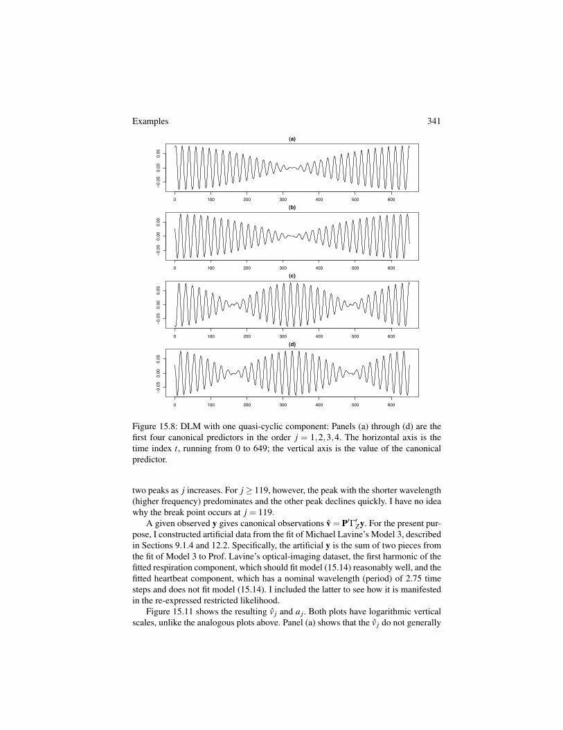
Examples 341
0 100 200 300 400 500 600
−0.0
50.
000.
05
(a)
Index
0 100 200 300 400 500 600
−0.0
50.
000.
05
(b)
Index
0 100 200 300 400 500 600
−0.0
50.
000.
05
(c)
Index
0 100 200 300 400 500 600
−0.0
50.
000.
05
(d)
Figure 15.8: DLM with one quasi-cyclic component: Panels (a) through (d) are thefirst four canonical predictors in the order j = 1,2,3,4. The horizontal axis is thetime index t, running from 0 to 649; the vertical axis is the value of the canonicalpredictor.
two peaks as j increases. For j � 119, however, the peak with the shorter wavelength(higher frequency) predominates and the other peak declines quickly. I have no ideawhy the break point occurs at j = 119.
A given observed y gives canonical observations v = P0G0Zy. For the present pur-
pose, I constructed artificial data from the fit of Michael Lavine’s Model 3, describedin Sections 9.1.4 and 12.2. Specifically, the artificial y is the sum of two pieces fromthe fit of Model 3 to Prof. Lavine’s optical-imaging dataset, the first harmonic of thefitted respiration component, which should fit model (15.14) reasonably well, and thefitted heartbeat component, which has a nominal wavelength (period) of 2.75 timesteps and does not fit model (15.14). I included the latter to see how it is manifestedin the re-expressed restricted likelihood.
Figure 15.11 shows the resulting v j and a j. Both plots have logarithmic verticalscales, unlike the analogous plots above. Panel (a) shows that the v j do not generally
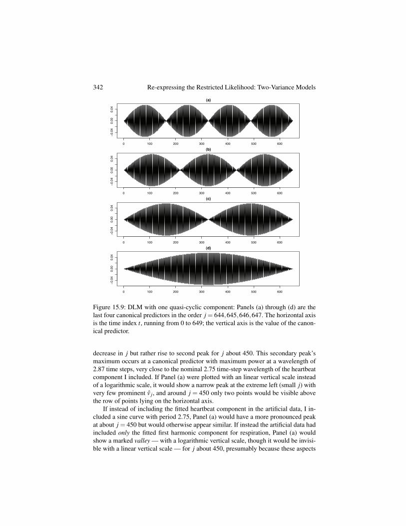
342 Re-expressing the Restricted Likelihood: Two-Variance Models
0 100 200 300 400 500 600
−0.0
40.
000.
04
(a)
Index
0 100 200 300 400 500 600
−0.0
40.
000.
04
(b)
Index
0 100 200 300 400 500 600
−0.0
40.
000.
04
(c)
Index
0 100 200 300 400 500 600
−0.0
40.
000.
04
(d)
Figure 15.9: DLM with one quasi-cyclic component: Panels (a) through (d) are thelast four canonical predictors in the order j = 644,645,646,647. The horizontal axisis the time index t, running from 0 to 649; the vertical axis is the value of the canon-ical predictor.
decrease in j but rather rise to second peak for j about 450. This secondary peak’smaximum occurs at a canonical predictor with maximum power at a wavelength of2.87 time steps, very close to the nominal 2.75 time-step wavelength of the heartbeatcomponent I included. If Panel (a) were plotted with an linear vertical scale insteadof a logarithmic scale, it would show a narrow peak at the extreme left (small j) withvery few prominent v j, and around j = 450 only two points would be visible abovethe row of points lying on the horizontal axis.
If instead of including the fitted heartbeat component in the artificial data, I in-cluded a sine curve with period 2.75, Panel (a) would have a more pronounced peakat about j = 450 but would otherwise appear similar. If instead the artificial data hadincluded only the fitted first harmonic component for respiration, Panel (a) wouldshow a marked valley — with a logarithmic vertical scale, though it would be invisi-ble with a linear vertical scale — for j about 450, presumably because these aspects
A Tentative Collection of Tools 343
0 100 200 300 400 500 600
010
2030
4050
j
Period
Figure 15.10: DLM with one quasi-cyclic component: The vertical axis is the period(wavelength) with the largest power in the jth canonical predictor’s power spectrum.
of Prof. Lavine’s data series had been captured in the fitted heartbeat componentand were thus deficient in the respiration component’s fit. (An exercise asks you toconstruct these two artificial datasets and draw the plots.)
These plots suggest how the restricted likelihood might be affected if the modeldoes not fit because of an omitted quasi-cyclic component. Recalling that the re-expressed restricted likelihood is a generalized linear model with gamma errors,“observations” v2
j , and linear predictor s
2s a j +s
2e , Figure 15.11 suggests that if the
omitted quasi-cyclic component has a higher nominal frequency than the includedcomponent, the lack of fit might tend to reduce the included component’s estimateds
2s . But what if the omitted component has a lower nominal frequency than the in-
cluded component? For artificial data consisting of Model 3’s fitted first harmonic forrespiration plus the fitted first harmonic for mystery (with nominal period 117 timesteps), the analog to Figure 15.11’s Panel (a) again shows a peak at the far left ofthe plot but also, surprisingly, a second and somewhat higher peak centered at aboutj = 100. Obviously a good deal of exploration remains to be done here.
15.3 A Tentative Collection of Tools
I learned that the re-expressed restricted likelihood for two-variance models is a gen-eralized linear model just before I started writing this chapter, so I have had littletime to work with that idea. Chapter 17 shows two classes of models for which therestricted likelihood can be re-expressed in a diagonalized or scalar-ized form asabove but for which the re-expressed restricted likelihood is not a generalized linearmodel with linear predictor a linear function of the unknowns in f . Thus, while thegeneralized linear model interpretation has been fruitful, it is probably not the lastword here.
344 Re-expressing the Restricted Likelihood: Two-Variance Models
0 100 200 300 400 500 600
1e−0
81e
−02
(a)
j
v−ha
t^2
0 100 200 300 400 500 600
110
100
10000
(b)
j
a_j
Figure 15.11: Artificial data fit with two quasi-cyclic components, fit using a DLMwith one quasi-cyclic component: Panel (a), v2
j ; Panel (b), a j.
Tools from generalized linear models. Generalized linear models provide severaltools: The deviance (a measure of goodness of fit, Section 2.3 in McCullagh & Nelder1989), residuals defined in various ways (Section 2.4), and measures of leverage(Section 12.7.1) and case influence (Section 12.7.3) that generalize the analogousmeasures for ordinary linear models. In the following chapters, I use only residualsand case-influence measures, modifying the latter to explore which canonical ob-servations v j provide information primarily about s
2s and which provide information
primarily about s
2e . Regarding deviance, I generally don’t find omnibus goodness-of-
fit tests useful because the important question is not whether a model fits but whetherits deficiencies of fit affect the answers to the subject-matter questions under study(cf Wakefield 1998, Critchley 1998), and goodness-of-fit tests do not reliably indicatethis. However, deviance is used for other purposes and it could be that a goodness-of-fit test applied to the restricted likelihood can identify occasions when more detailedexploration is likely to be useful. An exercise considers this possibility.
The canonical observations v j and their conditional variances s
2s a j+s
2e . Discrepant
canonical observations v j can be identified by computing v j/p
s
2s a j +s
2e with the
two variances replaced by estimates. Also, because var(v j|s2s ,s
2e ) = s
2s a j +s
2e , it
A Tentative Collection of Tools 345
seems obvious that mixed terms with very small a j generally provide informationonly about s
2e because s
2s has a negligible effect on v j unless s
2s is very large or s
2e
is very small. By the same heuristic reasoning, mixed terms with large a j provideinformation mainly about s
2s . These considerations are developed in Section 16.1.
A modified restricted likelihood that omits all j > m. To identify which mixed termsprovide information about which variance, I have found it useful to consider, forvarious m, a modified restricted likelihood that omits canonical observations j = m+1, . . . ,sZ +1, the last of these being the free terms. This is closely related to the caseinfluence of the group of “cases” j = m+1, . . . ,sZ +1, though usually case influenceanalyses consider only the effects of one or two cases. Also, I have found it usefulto consider the usual approximate standard errors computed from these modifiedrestricted likelihoods, which is also not usually part of case influence analysis.
The degrees of freedom in the fit for v j. Equation (15.7) is the conditional posteriordistribution given (s2
e ,s2s ) of the re-parameterized random effects v. In this con-
ditional posterior, the v j are independent with mean v j = v ja j/(a j + r), variances
2e a j/(a j + r), and DF a j/(a j + r) for r = s
2e /s
2s . These DF tell us about the con-
tributions the canonical predictors (GZP) j make to the fitted model, with larger DFindicating a greater contribution. Again, the a j are key: v j with large a j contributemore to the fit than v j with small a j, with the absolute sizes of the contributions de-termined by s
2s . As we’ll see in Chapter 16, these DF, along with an understanding
of which v j provide information about s
2s , explain why Section 14.3’s two smoothers
gave such different fits.
Reich & Hodges (2008a) emphasized two tools that are not listed here. Thosetools were helpful in understanding the examples described in that paper but nothelpful when applied to later examples, which led me to focus more on the v j andtheir conditional variances and on the modified restricted likelihood. One of the twodiscarded tools, called ri in Reich & Hodges (2008a), now appears entirely super-seded. The other discarded tool is a plot with vertical axis s
2s and horizontal axis
s
2e showing the lines s
2s = v2
j/a j �s
2s /a j (in the present chapter’s notation). The
jth such line describes the maximum of the jth mixed term; a vertical line for thefree terms was also drawn. This plot may turn out to have uses other than the onesin Reich & Hodges (2008a), so I am not yet ready to consign it to the trash heap ofhistory.
Exercises
Regular Exercises
1. (Section 15.1) Prove that GZ exists and give an expression for it.2. (Section 15.1) Show that the re-expressed restricted likelihood is invariant to the
choice of GZ .

346 Re-expressing the Restricted Likelihood: Two-Variance Models
3. (Section 15.1) Derive the joint posterior p(b ⇤,v,s2e ,s
2s |y) in equations (15.6) to
(15.9).4. (Section 15.2.2) Derive the re-expressed restricted likelihood for the full-rank
spline for the global-mean surface data and draw a contour plot of the log re-stricted likelihood. Compare your contour plot to Figure 15.3’s middle row leftpanel; your plot should look nearly identical except that it is shifted down bylog(4).
5. (Section 15.2.4) Derive the mixed-linear-model form for the dynamic linear modelgiven after equation (15.14).
6. (Section 15.2.4) Examine the canonical predictors for the dynamic linear model(15.14). You may wish to examine their power spectra, e.g., using the R functionspectrum. I find it remarkable how much their shapes change within the generalpattern of a gradually increasing frequency overlaid with other cyclic patterns,e.g., cyclically changing amplitude.
7. (Section 15.2.4) Re-draw Figure 15.11 for other artificial datasets. The text dis-cusses artificial datasets with a sine curve added to the fitted first harmonic forrespiration; consisting only of the fitted first harmonic for respiration; and con-sisting of Model 3’s fitted first harmonics for respiration and mystery.
Open Questions
1. (Section 15.2.3.2) Consider spatial confounding in the special case in which Fis exactly proportional to the kth column of V1. Suppose the true data-generatingmodel is y = 1nb0 +Fb +V(�k)
1 g + e and that some entries in g are big enoughin absolute value that s
2s has a large estimate. Can addition of the spatial random
effect S to the model y = 1nb0 +Fb + e change the estimate of b much or in-deed at all? As noted in the text, the key equations are (10.3) and (10.4) and thecomplication arises from the effect of rD in equation (10.4).
2. (Section 15.2.3.2) In the spatial-confounding problem, if the data are truly gen-erated by Model H, in which y = 1nb0 +Fb +Hg + e , how does H affect therestricted likelihood? The text discussed this qualitatively; examine this in detailby considering various H, g , and s
2e .
3. (Section 15.3) Interpreting the re-expressed restricted likelihood as a gamma-errors GLM, compute deviance-based goodness-of-fit tests for the penalizedspline, simple ICAR, and DLM examples. If this goodness-of-fit test is worth-while as a “gatekeeper” for deeper exploration, it should detect problems in thesimple ICAR fit to the attachment-loss data and the simple DLM fit to the artificialdatasets with quasi-cyclic components that are not in the model.