Embed Size (px)
Citation preview

MPRAMunich Personal RePEc Archive
A Common Factor Approach to SpatialHeterogeneity in AgriculturalProductivity Analysis
Markus Eberhardt and Francis Teal
Centre for the Study of African Economies (CSAE), Department ofEconomics, Oxford University
13. May 2009
Online at http://mpra.ub.uni-muenchen.de/15810/MPRA Paper No. 15810, posted 19. June 2009 05:50 UTC
A Common Factor Approach toSpatial Heterogeneity in
Agricultural Productivity Analysis∗
Markus Eberhardta,b† Francis Tealb
a St. John’s College, Oxfordb Centre for the Study of African Economies,
Department of Economics, University of Oxford
Draft: 13th May 2009
Abstract:
In this paper we investigate a ‘global’ production function for agriculture, using FAO data for 128countries from 1961-2002. Our review of the empirical literature in this field highlights that existingcross-country studies largely neglect variable time-series properties, parameter heterogeneity and thepotential for heterogeneous Total Factor Productivity (TFP) processes across countries. We motivatethe case for technology heterogeneity in agricultural production and present statistical tests indicatingnonstationarity and cross-section dependence in the data. Our empirical approach deals with thesedifficulties by adopting the Pesaran (2006) Common Correlated Effects estimators, which we extendby using alternative weight-matrices to model the nature of the cross-section dependence. We fur-thermore investigate returns to scale of production and production dynamics. Our results support thespecification of a common factor model in intercountry production analysis, highlight the rejection ofconstant returns to scale in pooled models as an artefact of empirical misspecification and suggest thatagro-climatic environment, rather than neighbourhood or distance, drives similarity in TFP evolutionacross countries. The latter finding provides a possible explanation for the observed failure of technol-ogy transfer from advanced countries of the temperate ‘North’ to arid and/or equatorial developingcountries of the ‘South’.
∗We are grateful to Stephen Bond for helpful comments and suggestions. Previous versions of this paper werepresented at the Gorman Student Research Workshop (December 2008), the CSAE Workshop, Department ofEconomics, University of Oxford (January 2009) and the CSAE annual conference (March 2009). All remainingerrors are our own. The first author gratefully acknowledges financial support during his doctoral studies fromthe ESRC, Award PTA-031-2004-00345.†Correspondence: St. John’s College, Oxford OX1 3JP; [email protected]
1
“[A]ssumptions of a common production function, and perfect and competitive factormarkets . . . get in the way of understanding international differences in productiv-ity — particularly differences between advanced and underdeveloped economies.”Nelson (1968, p.1229)
“Techniques developed in advanced countries were not generally directly transferableto less developed countries with different climates and resource endowments.”Ruttan (2002, p.162)
Ever since Hayami and Ruttan (1970) introduced the use of panel data to estimate cross-country production functions for the agriculture sector, academic studies have emphasised theconceptual desirability of technology heterogeneity across the diverse range of agro-climaticenvironments across countries. The literature further highlighted the potential for barriers totechnology transfer between countries which are specific to the agricultural sector, in particularthe problems of transfers between the developed countries of the temperate ‘North’ and thedeveloping countries of the arid or equatorial ‘South’: innovations in the former did not seemto yield the desired productivity boost in the latter context. In practice, however, empiricalinvestigation was typically based on models which impose technology homogeneity across thediverse sample of countries under analysis, or only allowed for heterogeneity by splitting thesample into crude geographical groups of countries. Further to this choice of empirical speci-fication, many studies opted to impose constant returns to scale on their regressions, despiteconcerns that the supply of one factor input, land, is essentially fixed.
In this paper we extend the insights gained from the emerging literature on multi-factor modelsin nonstationary panels (Bai & Ng, 2004; Coakley, Fuertes, & Smith, 2006; Pesaran, 2006;Kapetanios, Pesaran, & Yamagata, 2008) to cross-country empirical productivity analysis inthe agricultural sector — to the best of our knowledge this is the first empirical study to do so.We adopt a common factor model approach and estimate production functions for a panel of128 developing and developed countries using annual data from 1961 to 2002 (FAO, 2007). Ourfocus is on the changes in the parameter estimates and diagnostic tests when we move betweenpooled and heterogeneous estimators, between methods which ignore cross-section dependenceand those which accommodate it, and between approaches that put different emphasis on thetime-series properties of long T panels. This aside, the nature of the data for agriculture allowsus to investigate the cross-section dependence properties in a formal manner.
1
These innovations aside we particularly focus on three issues: firstly, we do not restrict thereturns to scale of production, given that with a fixed input (land) part of the production func-tion we do not have any priors about whether returns can assumed to be constant, decreasingor increasing.
Secondly, in an extension to the Pesaran (2006) common correlated effects estimators, we setout to identify what these ‘common effects’ might actually represent in the case of agriculture.In the standard CCE approach the nature of the cross-sectional dependence across countriesis unspecified; in our extension to this approach, which we believe represents a further orig-inal contribution to the empirical literature, we apply a number of weighting schemes in theconstruction of the cross-section averages, based on neighbourhood, geographical distance andagro-climatic distance. The application of weight matrices in essence imposes more structureon the factor loadings across countries, which in the standard CCE estimators are left uncon-strained. The first two of our extensions investigated essentially mimic standard spatial econo-metric approaches using geographical distance measures, the third represents a more complexcross-section correlation. The economic interpretation of our extension would be that the setof unobserved factors influencing productivity in each country is the same for its neighbours,countries in close(r) proximity or countries with similar agro-climatic environment respectively.Thus, countries that are not neighbours, are geographically more distant or have a very dis-similar agro-climatic conditions are argued to to be driven by different sets of factors.
Thirdly, we check the robustness of our empirical results by comparing them with those derivedfrom a dynamic specification of the production function. Again, the majority of studies in theliterature concentrate on static models.
Our empirical analysis thus investigates the interplay and salience of time-series properties ofthe data, parameter heterogeneity, returns to scale assumptions and the presence as well aspotential structure of cross-section dependence in the estimation of cross-country productionfunctions in agriculture.
The remainder of the paper is organised as follows: Section 1 briefly reviews the existingliterature on cross-country production function estimation for agriculture. Section 2 presentsa number of graphs to highlight agro-climatic heterogeneity across our sample of 128 countriesand provides the motivation for the empirical approach. Section 3 introduces the empiricalmodel adopted, develops our extension to the Pesaran (2006) CCE estimators and introducesthe data. Section 4 presents and discusses the empirical results,1 before we conclude our findingsin Section 5.
1The analysis of data time-series and cross-section dependence properties is presented in Appendices B andC respectively.
2

1 Literature review
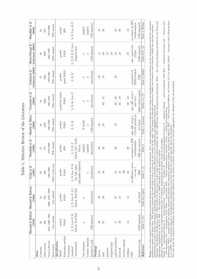
Following the seminal contribution by Hayami and Ruttan (1970) and a later update by thesame authors (Hayami & Ruttan, 1985), the literature on agricultural productivity analysisacross countries using panel data or ‘repeated cross-sections’ can be broadly distinguished bytwo aspects. The first of these does not relate to methodological approach, but to the datasetused, whereas the second major aspect relates to the empirical restrictions placed on pro-duction technology: whether countries are allowed to have differential technology parameters,TFP levels and evolvement, and whether constant returns to scale are imposed. While our shortoverview of the literature claims by no means to be exhaustive, we believe that the indicativeliterature presented in Table 1 and briefly discussed below does represent the breadth of theempirical field at the present time.
Most cross-country studies on agriculture use the data provided by the Food and AgricultureOrganisation (FAO) which provides output and input variables for a large number of countriesfrom 1961 onwards but relies on tractors and agricultural machinery as proxy for agriculturalcapital. Examples include Craig, Pardey, and Roseboom (1997); Cermeno, Maddala, and True-blood (2003); Bravo-Ortega and Lederman (2004) and Fulginiti, Perrin, and Yu (2004). Thealternative to this is a dataset developed by a World Bank team of researchers which providesagricultural fixed capital stock data for a maximum of 57 developing and developed countries(although in practice only 37 or 48 countries are used) from 1967-1992 (Larson, Butzer, Mund-lak, & Crego, 2000).2 An updated version of the dataset provides agricultural fixed capitalstock from 1972-2000 for 30 countries.3 The use of the two World Bank datasets is to ourknowledge limited to Mundlak, Larson, and Butzer (1997, 1999), as well as Martin and Mitra(2002), Gutierrez and Gutierrez (2003) and Mundlak, Larson, and Butzer (2008).
We highlight this difference since with the noteworthy exception of Martin and Mitra (2002)all empirical studies which use the World Bank dataset(s) obtain very high capital coefficients,typically between .35 and .6. The Martin and Mitra (2002) paper arrives at a much lowercoefficient of .12.4 In contrast, all studies using the FAO data with tractors proxying for fixedcapital stock obtain capital coefficients in the range .05 to .2.
The second major aspect relating to technology heterogeneity has commonly been limited tothe modelling of TFP. Technology parameter heterogeneity across countries has either been ig-nored (Hayami & Ruttan, 1970; Craig et al., 1997; Mundlak et al., 1999; Martin & Mitra, 2002;Mundlak et al., 2008) or approached by splitting the sample into ‘homogeneous groups’, e.g.by level of development (Hayami & Ruttan, 1985; Cermeno et al., 2003; Gutierrez & Gutier-rez, 2003). Although many of these studies stress the importance of allowing for technologydifferences across country groups, none of them investigates this in an approach which allowsfor full technology heterogeneity.
2Other variables, such as sectoral value added, arable land and agricultural are taken from World Bank,FAO and the ILO data (see Martin & Mitra, 2002).
3At present the updated data is not publicly available, although the it seems the World Bank team headedby Don Larson is happy to provide the data if approached.
4Given that the methods applied are very similar this discrepancy may be caused by the alternative deflationstrategy applied in Martin and Mitra (2002). Similar to the practice in the FAO data, the authors advocatethe use of a single LCU-US$ exchange rate (in their case for 1990) in favour of the practice of using annualexchange rates as implemented in the Larson et al. (2000) data.
3
Closely linked to the empirical specification of production technology is the returns to scaleassumption imposed on the regression model or tested. The underlying returns to scale of agri-cultural production affect the size-distribution of farms within an economy (Mundlak, Larson,& Crego, 1997). However, in addition we can think of a number of constraints, for instanceinsecure legal environment and variations in land tenure arrangements, that influence both ofthese processes in a similar fashion. For cross-country production analyses in agriculture find-ings of increasing, decreasing or constant returns to scale (all of which are present as can beseen in Table 1) are typically justified with reference to micro-economic studies of production orthe structural change within countries witnessed over the sample period. Hayami and Ruttan(1985), for instance, report increasing returns to scale for a subsample of developed countries(DC),5 while their developing country (LDC) sample cannot reject constant returns. Theyargue that increasing returns are linked to the indivisibility of fixed capital, which has playedan increasingly important role in the substitution of labour in developed countries (labour-saving technology). The result for their LDC sample is said to be the outcome of increasingpopulation pressure on land over the sample period, resulting in a decline in the land-labourratio. Efforts to increase productivity were therefore directed toward saving land by apply-ing more inputs that acted as land-substitutes, such as fertilizer, chemicals or improved seeds(land-saving technology). Since these inputs are highly divisible, the authors argue, it is notsurprising to encounter constant returns in this subsample. Although some LDCs also wit-nessed labour-saving technological change, it is argued that this must have been dominated bythe scale-neutral impact of land-saving technical change.
Mundlak, Larson, and Butzer (1997) in contrast argue that the “contribution of inputs togrowth should be judged by their contribution to output under a constant technology, attribut-ing the rest of the growth to technical change [TFP]” (paper summary). Their specification“succeeds in capturing the impact of cross-country differences in technology and thus eliminatesthe spurious result of increasing returns to scale.” (p.13)
With regard to our own analysis it is important to point out that once the empirical imple-mentation allows for heterogeneous technology across countries, the standard ceteris paribusproperty of regression parameters alluded to by Mundlak, Larson, and Butzer (1997) breaksdown. The implications are beyond the scope of this paper.
The study by Gutierrez and Gutierrez (2003) to the best of our knowledge represents the onlyanalysis which accounts for time-series properties of the data (nonstationarity, cointegration),using nonstationary panel econometric methods (Kao, Chiang, & Chen, 1999). Phillips andMoon (1999) have shown that even panel regressions can lead consistent ‘long-run average’estimates even if the error terms are nonstationary, such that the danger nonsense ‘spurious’regression is mitigated in the panel (Fuertes, 2008)— a result which depends on the units of thepanel being independent of each other. As in common with the vast majority of cross-countryempirical analysis, none of the studies reviewed considers the impact of cross-section dependencein the data on empirical estimates. The presence of such dependence can result in misleadinginference and even inconsistency in standard fixed effects panel estimators favoured in thisliterature (Phillips & Sul, 2003). Furthermore, if common factors drive both the regressors andthe error terms this will lead to inconsistent panel estimators due to the correlation betweenthe regressors and the error components (Pesaran, 2006).
5Only if data is deflated by the number of farms. They remark that their national aggregate data howeverdisplays constant returns for both subsamples — unfortunately results are not presented.
4
Tab
le1:
Sel
ecti
veR
evie
wof
the
Lit
erat
ure
Hayam
i&
Ru
ttan
Hayam
i&
Ru
ttan
Cra
iget
al
Mu
nd
lak
et
al
Mart
in&
Mit
raC
erm
en
oet
al
Gu
tierr
ez
&B
ravo-O
rtega
&M
un
dla
ket
al
(1970)
(1985)
(1997)
(1999)
(2002)
(2003)
Gu
tierr
ez
(2003)
Led
erm
an
(2004)
(2008)
Data
Cou
ntr
ies
3643
9837
4984
4786
30
Obse
rvat
ions
108
129
588
777
1248
2604
1081
2993
870
Yea
r(s)
/Per
iod
1955
,19
60,
1965
1960
,19
70,
1980
1961
-199
019
70-1
990
1967
-199
219
61-1
991
1970
-199
219
61-1
997
1972
-200
0
Dat
aso
urc
eow
n,
annual
own,
annual
FA
O,
5-ye
arav
g.W
B,
annual
WB
,an
nual
FA
O,
annual
WB
,an
nual
FA
O,
annual
WB
,an
nual
Spec
ifica
tion
Model
pool
edp
ool
edp
ool
edp
ool
edp
ool
edp
ool
edby
regi
onp
ool
edp
ool
edp
ool
ed
Est
imat
ion
met
hod
PO
LS
PO
LS
PO
LS
2FE
PO
LS
PO
LS
pan
elD
OL
SP
OL
S2F
E
Cov
aria
tes:
‘sta
ndar
d’
L,
N,
Liv
e,F
,K
L,
N,
Liv
e,F
,K†
L,
N,
Liv
e,F
,K
L,
N,
K,
FL
,N
,K
L,
N,
K,
Liv
e,F
L,
N,
KL
,N
,P
,K
,F
,L
ive,
L,
N,
Liv
e,K
,F
‘non
-sta
ndar
d’
Sch
ool
,T
ech
Edu
Sch
ool
,T
ech
Edu
Lit
,L
ife,
Infr
aSch
ool
,D
ev,
Yie
ld,
irri
gate
dla
nd
(all
qual
ity-a
dju
sted
)P
rice
s
Yea
rdum
mie
sX
Xim
plici
tN
tren
ds
XX
Xim
plici
t
Cou
ntr
ydum
mie
sX
implici
tX
XX
Xim
plici
t
Ret
urn
sto
scal
eC
RS
imp
osed
unre
stri
cted
unre
stri
cted
unre
stri
cted
CR
Sim
pos
edunre
stri
cted
unre
stri
cted
CR
Sim
pos
edC
RS
imp
osed
Fin
din
gs
lab
our
.40
.50
.25
.08
.64
.29
.11
.12
land
.07
.03
.40
.42
.24
.02
–.4
7.1
4.0
4.3
3
pas
ture
s.5
3
irri
gate
dla
nd
.03
capit
al/m
achin
ery
.11
.07
.05
.36
.12
.02
–.0
8.5
8.0
4.3
4
live
stock
.29
.31
.35
.03
–.4
0.2
5.0
8
trac
tion
anim
als
-.06
fert
iliz
er.1
4.1
5.0
4.0
8.0
0–
.10
.05
.13
TF
Pno
diff
eren
ceac
ross
acco
unte
dvia
2FE
sign
.diff
.ac
rossi,
sign
.diff
.ac
rossi
acco
unte
dvia
sign
.tr
end
term
acco
unte
dvia
2FE
ior
overt
tran
sfor
mat
ion
1.4-
3.5%
grow
thpa
and
overt
DO
LS
met
hod
(1%
pa)
tran
sfor
mat
ion
Ret
urn
sto
scal
e(C
RS
imp
osed
)not
test
edD
RS
CR
Snot
reje
cted
not
test
eddiff
ers
acro
ssre
gion
sC
RS
(CR
Sim
pos
ed)
(CR
Sim
pos
ed)
Refe
ren
ceT
able
2,(1
7)T
able
6-2,
(Q14
)T
able
1,(1
)T
able
4T
able
1,fo
otnot
eT
able
s1-
4,(7
)T
able
2,D
OL
ST
able
6(A
),(2
)T
able
2,W
ithin
Notes:
The
table
com
pare
sC
obb-D
ougla
spro
ducti
on
functi
on
est
imate
sfr
om
studie
sas
indic
ate
d.
Sin
ce
many
studie
sre
port
resu
lts
for
more
than
one
specifi
cati
on
we
concentr
ate
on
the
most
genera
lm
odel
for
‘sta
ndard
’pro
ducti
on
inputs
wit
hpanel
data
.T
he
specifi
cre
fere
nce
for
each
study’s
entr
yis
state
dat
the
bott
om
of
the
table
.T
he
studie
sby
Hayam
iand
Rutt
an
(1985)
and
Guti
err
ez
and
Guti
err
ez
(2003)
als
opro
vid
ese
para
teest
imati
ons
by
countr
ygro
ups
(develo
ped,
develo
pin
g),
findin
gpro
ducti
on
technolo
gy
diff
ere
nces
tob
econsi
dera
ble
and
negligib
lere
specti
vely
.D
ata
sets
:T
he
Hayam
iand
Rutt
an
(1970,
1985)
studie
suse
data
from
aw
ider
range
of
sourc
es
whic
hin
clu
des
the
FA
O,
OE
CD
and
oth
er
inte
rnati
onal
inst
ituti
ons.
FA
O—
the
vari
ous
data
base
spro
vid
ed
by
the
Food
and
Agri
cult
ure
Org
anis
ati
on
of
the
UN
,W
B—
the
Lars
on
et
al.
(2000)
data
set
and
its
up
date
dvers
ion.
Outp
ut
isagri
cult
ura
loutp
ut
(expre
ssed
inso
me
typ
eof
const
ant
‘inte
rnati
onal’
moneta
ryte
rms)
inall
studie
s.In
puts
:L
—agri
cult
ura
lla
bour,
N—
(cro
p)
land,
Liv
e—
livest
ock,
F—
fert
iliz
er,
K—
capit
al
stock/m
achin
ery
/tr
acto
rs,
P—
past
ure
s,School
—sc
hool
enro
lment,
Tech
Edu
—te
chnic
al
educati
on,
Lit
—lite
racy,
Lif
e—
life
exp
ecta
ncy,
Dev
—develo
pm
ent
level,
Yie
ld—
peak
yie
ld,
Infr
a—
vari
ous
infr
ast
ructu
revari
able
s,P
rices
—vari
ous
pri
ce
indic
ato
rs.
Est
imato
rs:
PO
LS
—p
oole
dO
LS
(we
indic
ate
separa
tely
wheth
er
the
regre
ssio
nequati
on
conta
ins
countr
yfi
xed
eff
ects
),2F
E—
Tw
o-w
ay
Fix
ed
Eff
ects
,se
eSecti
on
3.2
.1fo
rdeta
ils,
DO
LS
—D
ynam
icO
LS,
follow
ing
Kao
et
al.
(1999).
This
est
imato
rim
pose
sa
hom
ogeneous
coin
tegra
tion
vecto
rbut
allow
sfo
rcountr
y-s
pecifi
csh
ort
-run
dynam
ics.
†For
this
study
the
rep
ort
ed
coeffi
cie
nts
are
deri
ved
from
data
defl
ate
dby
the
num
ber
of
farm
s.R
egre
ssio
ns
for
nati
onal
aggre
gate
sare
alluded
tobut
not
pre
sente
d.
5
2 Technology Heterogeneity and the Analysis of
Agricultural Production
2.1 Heterogeneity in the Agro-Climatic Environment
In this section we attempt to create an impression of the differential agro-climatic environmentacross different countries. Our focus is here on the differences in the share of arable land6 inclimatic zones across regions of the globe. The data is taken from FAO (2007) and Gallup,Mellinger, and Sachs (1999). The sample is made up of 128 developing and developed coun-tries; the measures presented are essentially time-invariant. Detailed information about dataconstruction and sample coverage is presented in Appendix A.
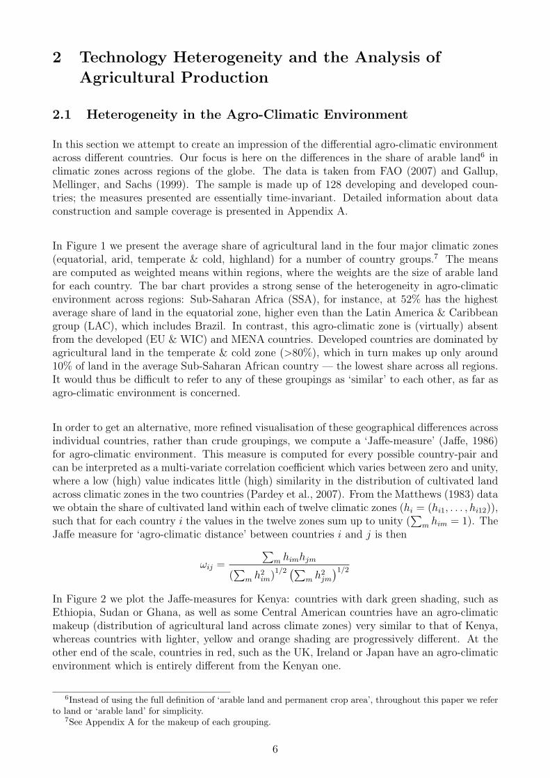
In Figure 1 we present the average share of agricultural land in the four major climatic zones(equatorial, arid, temperate & cold, highland) for a number of country groups.7 The meansare computed as weighted means within regions, where the weights are the size of arable landfor each country. The bar chart provides a strong sense of the heterogeneity in agro-climaticenvironment across regions: Sub-Saharan Africa (SSA), for instance, at 52% has the highestaverage share of land in the equatorial zone, higher even than the Latin America & Caribbeangroup (LAC), which includes Brazil. In contrast, this agro-climatic zone is (virtually) absentfrom the developed (EU & WIC) and MENA countries. Developed countries are dominated byagricultural land in the temperate & cold zone (>80%), which in turn makes up only around10% of land in the average Sub-Saharan African country — the lowest share across all regions.It would thus be difficult to refer to any of these groupings as ‘similar’ to each other, as far asagro-climatic environment is concerned.
In order to get an alternative, more refined visualisation of these geographical differences acrossindividual countries, rather than crude groupings, we compute a ‘Jaffe-measure’ (Jaffe, 1986)for agro-climatic environment. This measure is computed for every possible country-pair andcan be interpreted as a multi-variate correlation coefficient which varies between zero and unity,where a low (high) value indicates little (high) similarity in the distribution of cultivated landacross climatic zones in the two countries (Pardey et al., 2007). From the Matthews (1983) datawe obtain the share of cultivated land within each of twelve climatic zones (hi = (hi1, . . . , hi12)),such that for each country i the values in the twelve zones sum up to unity (
∑m him = 1). The
Jaffe measure for ‘agro-climatic distance’ between countries i and j is then
ωij =
∑m himhjm
(∑
m h2im)
1/2 (∑m h
2jm
)1/2In Figure 2 we plot the Jaffe-measures for Kenya: countries with dark green shading, such asEthiopia, Sudan or Ghana, as well as some Central American countries have an agro-climaticmakeup (distribution of agricultural land across climate zones) very similar to that of Kenya,whereas countries with lighter, yellow and orange shading are progressively different. At theother end of the scale, countries in red, such as the UK, Ireland or Japan have an agro-climaticenvironment which is entirely different from the Kenyan one.
6Instead of using the full definition of ‘arable land and permanent crop area’, throughout this paper we referto land or ‘arable land’ for simplicity.
7See Appendix A for the makeup of each grouping.
6
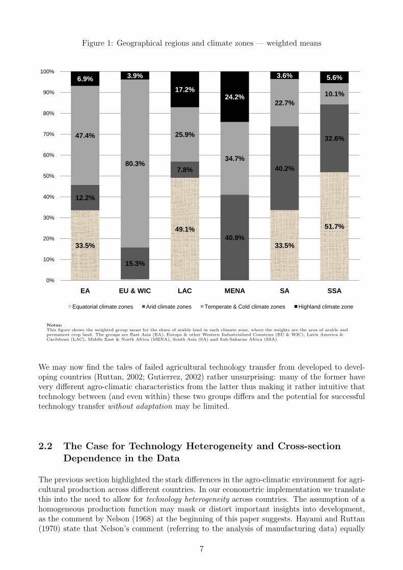
Figure 1: Geographical regions and climate zones — weighted means
50.5%
67.2%
37.8%
54.8%
4.4%
4.2%
2.4%
40.7%
27.7%
28.9%
38.0%
91.2%
14.3%
42.2%
20.0%
13.1%
7.1% 4.4%
16.2% 17.2% 14.6%
3.1%
0%
10%
20%
30%
40%
50%
60%
70%
80%
90%
100%
EA EU & WIC LAC MENA SA SSA
Equatorial climate zones Arid climate zones Temperate & Cold climate zones Highland climate zone
33.5%
49.1%
33.5%
51.7%
12.2%
15.3%
7.8%
40.9%
40.2%
32.6%47.4%
80.3%
25.9%
34.7%
22.7%
10.1%
6.9% 3.9%
17.2%24.2%
3.6% 5.6%
0%
10%
20%
30%
40%
50%
60%
70%
80%
90%
100%
EA EU & WIC LAC MENA SA SSA
Equatorial climate zones Arid climate zones Temperate & Cold climate zones Highland climate zone
Notes:This figure shows the weighted group mean for the share of arable land in each climate zone, where the weights are the area of arable andpermanent crop land. The groups are East Asia (EA), Europe & other Western Industrialised Countries (EU & WIC), Latin America &Caribbean (LAC), Middle East & North Africa (MENA), South Asia (SA) and Sub-Saharan Africa (SSA).
We may now find the tales of failed agricultural technology transfer from developed to devel-oping countries (Ruttan, 2002; Gutierrez, 2002) rather unsurprising: many of the former havevery different agro-climatic characteristics from the latter thus making it rather intuitive thattechnology between (and even within) these two groups differs and the potential for successfultechnology transfer without adaptation may be limited.
2.2 The Case for Technology Heterogeneity and Cross-sectionDependence in the Data
The previous section highlighted the stark differences in the agro-climatic environment for agri-cultural production across different countries. In our econometric implementation we translatethis into the need to allow for technology heterogeneity across countries. The assumption of ahomogeneous production function may mask or distort important insights into development,as the comment by Nelson (1968) at the beginning of this paper suggests. Hayami and Ruttan(1970) state that Nelson’s comment (referring to the analysis of manufacturing data) equally
7
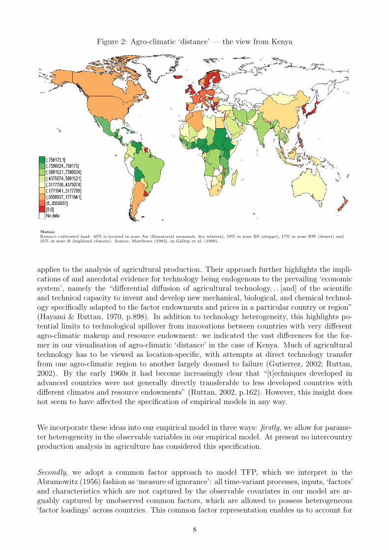
Figure 2: Agro-climatic ‘distance’ — the view from Kenya
Notes:Kenya’s cultivated land: 40% is located in zone Aw (Equatorial savannah, dry winters), 19% in zone BS (steppe), 17% in zone BW (desert) and25% in zone H (highland climate). Source: Matthews (1983), in Gallup et al. (1999).
applies to the analysis of agricultural production. Their approach further highlights the impli-cations of and anecdotal evidence for technology being endogenous to the prevailing ‘economicsystem’, namely the “differential diffusion of agricultural technology. . . [and] of the scientificand technical capacity to invent and develop new mechanical, biological, and chemical technol-ogy specifically adapted to the factor endowments and prices in a particular country or region”(Hayami & Ruttan, 1970, p.898). In addition to technology heterogeneity, this highlights po-tential limits to technological spillover from innovations between countries with very differentagro-climatic makeup and resource endowment: we indicated the vast differences for the for-mer in our visualisation of agro-climatic ‘distance’ in the case of Kenya. Much of agriculturaltechnology has to be viewed as location-specific, with attempts at direct technology transferfrom one agro-climatic region to another largely doomed to failure (Gutierrez, 2002; Ruttan,2002). By the early 1960s it had become increasingly clear that “[t]echniques developed inadvanced countries were not generally directly transferable to less developed countries withdifferent climates and resource endowments” (Ruttan, 2002, p.162). However, this insight doesnot seem to have affected the specification of empirical models in any way.
We incorporate these ideas into our empirical model in three ways: firstly, we allow for parame-ter heterogeneity in the observable variables in our empirical model. At present no intercountryproduction analysis in agriculture has considered this specification.
Secondly, we adopt a common factor approach to model TFP, which we interpret in theAbramowitz (1956) fashion as ‘measure of ignorance’: all time-variant processes, inputs, ‘factors’and characteristics which are not captured by the observable covariates in our model are ar-guably captured by unobserved common factors, which are allowed to possess heterogeneous‘factor loadings’ across countries. This common factor representation enables us to account for
8
cross-section dependence between countries — this dependence can be hypothesised to arisefrom common shocks and/or spillover effects, the latter determined for instance by trade, policyor technology (Costantinia & Destefanis, 2008). The importance of accounting for cross-sectiondependence in estimation and inference has become a major theme in the recent nonstation-ary panel econometric literature (Bai & Ng, 2004; Pesaran, 2004; Breitung & Pesaran, 2005;Coakley et al., 2006; Baltagi, Bresson, & Pirotte, 2007) and this paper represents our secondempirical example of these themes.
Thirdly, we use the above arguments of potential barriers to technology spillovers to motivatean extension to the Pesaran (2006) CCE estimators. In the standard setup these estimatorsaccount for the impact of unobserved factors by augmenting the regression equation with avector of cross-section averages at time t for each of the variables, whereby the averages areconstructed from equally weighted observations across all countries. The economic interpreta-tion of this approach would be that the set of unobserved factors which influences productivityis common to all countries — this is not to say that their impact is the same (in fact theirheterogeneity is the major contribution of the Pesaran (2006) approach), it is just required thatacross all countries the impact of each factor is on average non-zero. In our extension we choseto impose some more structure on this framework by investigating three alternative scenarios:
(i) The ‘Neighbourhood Effect’: many empirical studies have argued that the economicperformance of contiguous neighbours to country i has a significant effect on the latter’stotal factor productivity, and attempted to measure the impact of this spillover empiricallyby specifying spatially-lagged dependent variables in a production function model (e.g.Ertur & Koch, 2007). In our empirical models we will allow for a conceptually similarrelationship in the data using the alternative CCE estimation approach.
(ii) The ‘Gravity Model Effect’: gravity models are common in empirical trade analysiswhere they suggest geographical distance as a powerful determinant of the magnitude ofeconomic exchange between countries (e.g. Frankel & Romer, 1999; Redding & Venables,2004). We adopt this approach to hypothesise that distance between countries (a crudeproxy for factors such as climatic, soil, cultural, ethnic and socio-economic differences)can explain the effects of unobserved heterogeneity across countries. Existing examples inthe spatial econometric literature are reviewed in Magrini (2004), Abreu, de Groot, andFlorax (2005) and Bode and Rey (2006).
(iii) The ‘Agro-Climatic Distance Effect’: much of the existing literature on intercountryproduction functions in agriculture particularly highlights the differential agro-climaticcharacteristics across countries and even explicitly links the failure of technology trans-fer between diverse countries to heterogeneity in resource endowment and climate. Ourthird alternative to the standard CCE approach hypothesises that countries with similaragro-climatic makeup are influenced by similar unobserved factors.
In the following section we show somewhat more formally how these ideas are introduced intoour econometric model.
9
3 Empirical Model and Implementation
3.1 Common factor model representation
We adopt an unobserved common factor model as our empirical framework. For i = 1, . . . , Nand t = 1, . . . , T , let
yit = β′i xit + uit uit = αi + λ′i ft + εit (1)
xmit = πmi + δ′mi gmt + ρ1mi f1mt + . . .+ ρnmi fnmt + vmit (2)
where m = 1, . . . , k and f ·mt ⊂ ft
ft = %′ft−1 + et and gt = κ′gt−1 + εt (3)
We assume a production function with observed inputs xit (labour, agricultural capital stock,livestock, fertilizer, land under cultivation) and observed net output yit (all in logarithms).Technology parameters on the inputs can vary across countries (βi). Unobserved agriculturalTFP is represented by a combination of country-specific TFP levels αi and a set of commonfactors ft with factor loadings that can differ across countries (λ′i). We also introduce anempirical representation of the observed inputs in equation (2) in order to indicate the pos-sibility for endogeneity: the input variables xit are driven by a set of common factors gmt aswell as an additional set of factors fnmt, whereby the latter as indicated represent a subsetof the factors driving output in equation (1). The intuition is that some unobserved factorsdriving agricultural production are likely to similarly drive (at least in parts) the evolutionof the inputs. This overlap of common factors creates severe difficulties for the identificationof the technology parameters βi (see Remark 4 in Kapetanios et al., 2008) and our empiricalestimators set out to address this issue: previous simulation exercises (Coakley et al., 2006;Kapetanios et al., 2008) as well as our own investigations (available on request) indicate thatthe newly-developed CCE-type estimators are able to accommodate this type of endogeneity inthe estimation equation to arrive at consistent parameter estimates for common β coefficientsor the means of heterogeneous βi. Equation (3) indicates that the factors are persistent overtime, which allows for the setup to accommodate nonstationarity in the factors (% = 1, κ = 1)and thus the observables. It further allows for various combinations of cointegration: betweenoutput y and inputs x, and between output y, inputs x and (some of) the unobserved factorsft. The latter alternative is of particular interest, since it will allow us to specify a cointegratingrelationship without even knowing its individual elements.
The above empirical framework allows for the maximum level of flexibility, with regard toparameter heterogeneity, cross-section dependence induced by the common factors, and non-stationarity in the observables and unobserved factors.
3.2 Empirical estimators
3.2.1 Estimators imposing homogeneous parameters
We first use the full time-series of the data to estimate pooled OLS (POLS), two-way fixedeffects (2FE), and pooled OLS for data in first differences (FD-OLS). In order to capture theunobserved common processes the POLS and FD-OLS estimation equations contain a set ofT − 1 year dummies (in first differences in the FD-OLS equation); the 2FE estimator capturesthe common processes by transforming all variables into deviations from the cross-section mean.
10
Formally, the above estimators are defined as
POLS yit = a+ bxit +T∑s=2
csDs + eit (4)
FD-OLS ∆yit = b∆xit +T∑s=2
cs∆Ds + ∆eit (5)
2FE yit = bxit + eit (6)
where zit = zit− zi− zt + z with zi = T−1∑T
t=1 zit (country average), zt = N−1∑N
i=1 zit (cross-
section average) and z = (NT )−1∑T
t=1
∑Ni=1 zit (full sample average).
None of the above estimators explicitly addresses cross-section dependence in the data. Thisis addressed in the pooled version of the Pesaran (2006) Common Correlated Effects estimator(CCEP), where the pooled fixed effects equation is augmented by cross-section averages of thedependent and the independent variables, in a fashion such that the impact of the unobservedcommon factors is allowed to vary across countries. Formally,
CCEP yit = a+ bxit +N∑j=2
djDj +N∑j=1
c1i{ytDj}+N∑j=1
c2i{xtDj}+ eit (7)
where the first three terms represent a standard fixed effects estimator and the last two termsrepresent the augmentation with cross-section averages at time t (zt = N−1
∑Ni=1 zit) interacted
with a set of N country dummies Dj. This combination creates k + 1 matrices of dimensionsNT ×N where k is the number of observed variables in the model.
The intuition why this rather simple augmentation can do away with the impact of unobservedcommon factors (with heterogeneous factor loadings) is as follows: take the cross-section aver-ages of our hypothesised DGP in equation (1) for each point in time to yield
yt = α + β′xt + γ′ft (8)
⇔ ft = γ−1(yt − α− β′xt) since εt = 0
This indicates that provided the average impact of each factor across all countries is non-zero(γ 6= 0), the use of cross-section averages of the dependent (yt) and independent variables (xt)can act as a representation of the unobserved common factors ft since as the cross-sectiondimension (N) becomes large ft → ft in probability. To allow for heterogeneity in the factorloadings this representation must be implemented in the fashion outlined above.
Pesaran (2006) shows that the asymptotic consistency of the CCEP estimator is based on anyweighted cross-section aggregates (zt =
∑iwizit) provided the weights wi satisfy the condi-
tions
wi = O
(1
N
) N∑i=1
wiγi 6= 0N∑i=1
|wi| < K (9)
where K is a finite positive constant (Coakley et al., 2006). In the standard CCE estimatorthe weights are the same for all countries (1/N) as zt represents the arithmetic mean. In anextension to this standard practice we experiment with a number of weight-matrices to develop
11
alternative CCE estimators. We present three variants of the standard approach:
1. The Neighbourhood CCE approach — for country i the cross-section averages (means)for y and x are constructed from the values for i’s contiguous neighbours.
2. The Gravity CCE approach — for country i the observations for countries j = 1, . . . , N−1are weighted by the inverse of the population-weighted distance between i and j (theseweights were normalised so that they sum to unity) before computing the cross-sectionaggregate.
3. The Agro-Climatic CCE approach — for country i the observations for countries j =1, . . . , N−1 are weighted by Jaffe’s measure for agricultural distance (see below) betweeni and j (these weights were normalised so that they sum to unity) before computing thecross-section aggregate.8
Our conceptual justification for these variants of the CCEP (and also the CCEMG) estimatoris the situation where the average of factor loadings across countries is non-zero, but systematicpatterns drive the data. In the distance case we implicitly test the hypothesis that country iis driven by unobserved common factors which are the same in countries in close proximity,but is much less affected by other factors which drive countries further away from it. Theneighbourhood case represents an extreme extension of this argument whereby only countrieswhich share a common border are driven by the same factors. Finally, in the agro-climaticcase we test the hypothesis that countries with similar agro-climatic environment are affectedby a shared set of common factors, but that these countries are not (or only to a very limiteddegree) affected by a separate set of common factors, which in turn influences countries in verydifferent agro-climatic environments.
All of the above estimators impose parameter homogeneity on the production technology (ob-served variables) and TFP (unobserved common factors), with the exception of the CCEPestimator which allows for heterogeneity in TFP evolvement. If variables (y,x) and factors (f)are nonstationary the POLS, FE and 2FE estimators require that the cointegrating relationbetween y,x and f is homogeneous across countries. Similarly, if only y and x are nonsta-tionary their cointegrating relationship is required to be common across countries. As oursimulation study reveals9 the use of year dummies can greatly reduce the misspecification biasin a range of scenarios when these assumptions are violated, however the regression equationsfundamentally are misspecified and contain nonstationary errors.10 We now turn to a numberof estimators which allow for parameter heterogeneity in both the production technology andTFP evolvement.
3.2.2 Estimators allowing for parameter heterogeneity
All of the following estimators are based on individual country regressions. A starting pointis the Pesaran and Smith (1995) Mean Group estimator (MG) which assumes cross-sectionindependence (absence of unobserved common factors) and in the presence of nonstationaryvariable series requires heterogeneous cointegration, i.e. that the country regression model iscorrectly specified and encompasses the cointegrating relationship.
8For the Jaffe (1986) measure see Section 2.1 for details. For the distance and agro-climatic distance wenormalise the weights (across i) so that they sum to unity.
9Available on request.10The CCEP estimator seems to be the exception with regard to the latter.
12
We thus estimate N country regressions
MG yit = ai + bixit + cit+ eit (10)
bMG = N−1∑i
bi
where t is a linear trend term with parameter coefficient ci and ai is the intercept. By construc-tion all parameters can differ across countries, indicated by the subscript i. The linear trendterm is included to capture unobserved idiosyncratic processes which are time-invariant. TheMG estimates are then derived as averages of the individual country estimates.
3.2.3 Estimators allowing for parameter heterogeneity and common factors
We also present results for the Augmented Mean Group estimator (AMG), which we developedin Eberhardt and Teal (2008). This estimator accounts for potential cross-section dependence byinclusion of a ‘common dynamic effect’ in the country regression. This variable is extracted fromthe year dummy coefficients of the pooled regression in first differences and (following trans-formation) represents a levels-equivalent average evolvement of unobserved common factorsacross all countries. Provided that the unobserved common factors form part of the country-specific cointegrating relation, the augmented country regression model thus encompasses thecointegrating relationship, which is allowed to differ across countries.
AMG Stage (i) ∆yit = b∆xit +T∑s=2
cs∆Ds + ∆eit (11)
⇒ cs ≡ µ•tAMG Stage (ii) yit = ai + bixit + κiµ
•t + cit+ eit (12)
bAMG = N−1∑i
bi
The first stage represents a standard FD-OLS regression with T − 1 year dummies in firstdifferences, from which we collect the year dummy coefficients which are labelled as µ•t . Inthe second stage this variable is included in each of N standard country regression whichalso includes a linear trend term to capture unobserved idiosyncratic processes which are time-invariant. The AMG estimates are then derived as averages of the individual country estimates.
This approach is conceptually close to the Mean Group version of the Pesaran (2006) CommonCorrelated Effects (CCEMG) estimator, which is a variant on the pooled estimator CCEPintroduced above. For CCEMG we obtain N country regression equations, each of whichcontains the cross-section average terms for y and x
CCEMG yit = ai + bixit + c1iyt + c2ixt + eit (13)
bCCEMG = N−1∑i
bi
As was detailed above the cross-section averages can account for unobserved common factorswith heterogeneous factor loadings. The CCEMG estimates are then averaged across countries.We develop the three variants of the CCEMG estimator in analogy to the pooled estimatorcase.
13
3.3 Data
The principal data source for our empirical analysis is the Food and Agriculture Organisation’sFAOSTAT panel database (FAO, 2007), from which we obtain annual observations for agricul-tural net output, economically active labour force in agriculture, number of tractors used inagriculture, arable land and permanent crop land and fertilizer use in 128 countries from 1961to 2002 (average T = 40.3).
Additional time-invariant data on geographical distance between countries and contiguity (neigh-borhood) is taken from CEPII (2006), and data on the share of agricultural land by climaticzone from Matthews (1983) available in Gallup et al. (1999). Data construction is discussed inAppendix A which also contains the descriptive statistics.
4 Empirical Results
4.1 Time-Series Properties and Cross-Section Dependence
We carry out a set of stationarity and nonstationarity tests for individual country time-series aswell as the panel as a whole, results for which are presented in Appendix B. Ultimately, in caseof the present data dimensions and characteristics, and given all the problems and caveats ofindividual country and panel unit root tests, we can suggest most conservatively that nonsta-tionarity cannot be ruled out in this dataset. Investigation of the time-series properties of thedata was not intended to select a subset of countries which we can be reasonably certain displaynonstationary variable series like in Pedroni (2007); instead, our aim was to indicate that thesample (possibly due to the limited time-series dimension, as argued in Pedroni, 2007) is likelyto be made up of a mixture of some countries with stationary and others with nonstationaryvariable series.
The results for the cross-section dependence (CSD) analysis are presented in Appendix C. Ouranalysis provides strong evidence for the presence of cross-section dependence within the fullsample dataset, based on average variable cross-country correlation coefficients, principal com-ponent analysis and the Pesaran (2004) CD test. This result holds for both the individualvariables as well as residuals from regressions which do not address cross-section correlation:the pooled OLS (POLS), two-way fixed effects (2FE) and Mean Group (MG) estimators.11
The CD test for residuals from standard CCEMG regressions cannot reject cross-section in-dependence, indicating that this approach successfully deals with the presence of unobservedcommon factors. It is noteworthy that the average cross-section correlation for residuals fromthe pooled OLS regression with variables in first differences (FD-OLS) drops considerably andlike in the CCEMG case cross-section independence cannot be rejected. This result is surprising— Coakley et al. (2006) did not investigate the FD-OLS estimator in their study and we furthernoted its performance in our dedicated Monte Carlo analysis (available on request). We alsocarry out the same testing procedures for various subsamples of the data, based on geographicand climatic categories. The standard CCEMG estimator seems to achieve the elimination ofcross-section dependence even within and across narrower subsamples, while most other estima-tion approaches (now including FD-OLS) are subject to considerable residual correlation within
11POLS is augmented with T − 1 year dummies, MG country regressions with a linear trend term.
14
and across country groupings. CD tests and mean absolute residual correlation are reported inthe results section below for each of the empirical specifications considered.
4.2 Pooled estimation results
We present the estimation results for the pooled specifications in Table 2. The dependent vari-able and the independent variables are expressed in per worker term, such that the additionof the labour variable indicates deviation from constant returns to scale. In the lower panelsof the table we report the implied returns to scale and labour coefficients as well as variousdiagnostic test results. Recall for the following discussion that the 2FE estimator representsthe empirical implementation of choice in the present literature.
We first discuss parameter coefficients: most empirical models presented indicate large de-creasing returns to scale in agriculture. In common with many studies using the FAO data,the coefficients on capital (tractors) are relatively low across all models, ranging from .04 (FD-OLS) to .13 (POLS). The land coefficients are high and relatively stable across specifications(between .21 and .33), whereas the fertilizer coefficients range from .01 to .17. Livestock againhas a rather large coefficient across all specifications (.22 to .37).
Regarding the implied labour coefficients, we find very low magnitudes across all specifications,with the standard and distance-weighted CCEP even providing nonsensical negative parametervalues. Certainly the most striking pattern in these results is the general magnitude of theimplied decreasing returns to scale: based on this analysis we can conclude that in a pooledspecification the data in all but two of the weighted CCE estimators rejects constant returnsemphatically, with input elasticities in the commonly favoured 2FE estimator adding up toaround .80. This finding may reflect a global production function with substantial decreasingreturns to scale, possibly due to the presence of a fixed factor (median land per worker growthrate for the sample: 0.0%); alternatively, it may reflect empirical misspecification.
Turning to the diagnostics, we can see that with the exception of the models in first differences,all models seem to display serial correlation in the residuals. Unit root tests indicate that theCCEP-type and first difference estimators seem to yield stationary residuals, in contrast tothe standard panel estimators in levels (POLS, 2FE) for which nonstationary residuals cannotbe rejected. Recall that t-statistics are invalid in the presence of nonstationary errors (Kao,1999). Mean absolute residual correlations for POLS and 2FE are relatively high, at around.4, whereas this measure drops to around .16 in all other regression models. Nevertheless thePesaran (2004) CD-test for cross-section dependence yields very mixed results: only the residu-als for the agro-climate CCEP and the FD-OLS estimator suggest cross-section independence.Further specification tests emphatically reject residual normality and homoskedasticity in allmodels. These diagnostics indicate that the commonly preferred 2FE estimator has seriallycorrelated errors, which are nonstationary, nonnormal, heteroskedastic and correlated acrosscountries. Note that input parameter estimates for this estimator are reasonably close to thosein Craig et al. (1997), the closest match for this dataset and specification.
15
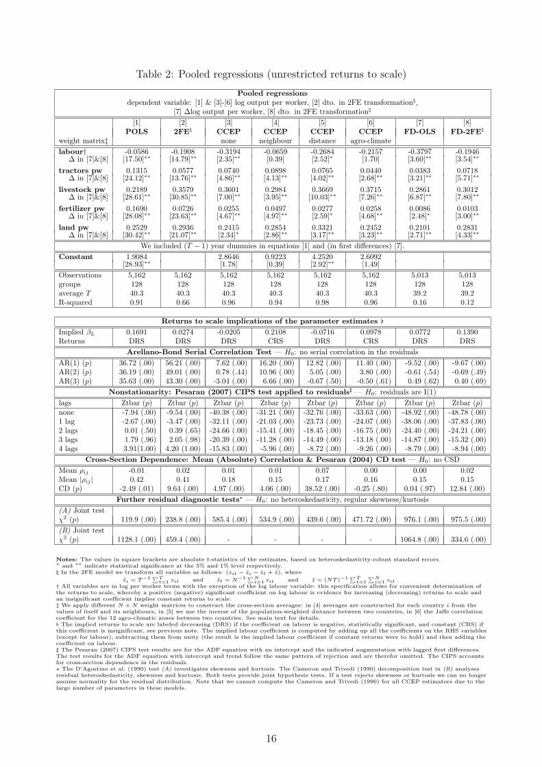
Table 2: Pooled regressions (unrestricted returns to scale)
Pooled regressionsdependent variable: [1] & [3]-[6] log output per worker, [2] dto. in 2FE transformation\,
[7] ∆log output per worker, [8] dto. in 2FE transformation\
[1] [2] [3] [4] [5] [6] [7] [8]POLS 2FE\ CCEP CCEP CCEP CCEP FD-OLS FD-2FE\
weight matrix‡ none neighbour distance agro-climatelabour† -0.0586 -0.1908 -0.3194 -0.0659 -0.2684 -0.2157 -0.3797 -0.1946
∆ in [7]&[8] [17.50]∗∗ [14.79]∗∗ [2.35]∗∗ [0.39] [2.52]∗ [1.70] [3.60]∗∗ [3.54]∗∗
tractors pw 0.1315 0.0577 0.0740 0.0898 0.0765 0.0440 0.0383 0.0718∆ in [7]&[8] [24.12]∗∗ [13.76]∗∗ [4.86]∗∗ [4.13]∗∗ [4.02]∗∗ [2.68]∗∗ [3.21]∗∗ [5.71]∗∗
livestock pw 0.2189 0.3579 0.3601 0.2984 0.3669 0.3715 0.2861 0.3012∆ in [7]&[8] [28.61]∗∗ [30.85]∗∗ [7.00]∗∗ [3.95]∗∗ [10.03]∗∗ [7.26]∗∗ [6.87]∗∗ [7.80]∗∗
fertilizer pw 0.1690 0.0726 0.0255 0.0497 0.0277 0.0258 0.0086 0.0103∆ in [7]&[8] [28.08]∗∗ [23.63]∗∗ [4.67]∗∗ [4.97]∗∗ [2.59]∗ [4.68]∗∗ [2.48]∗ [3.00]∗∗
land pw 0.2529 0.2936 0.2415 0.2854 0.3321 0.2452 0.2101 0.2831∆ in [7]&[8] [30.42]∗∗ [21.07]∗∗ [2.34]∗ [2.86]∗∗ [3.17]∗∗ [3.23]∗∗ [2.71]∗∗ [4.33]∗∗
We included (T − 1) year dummies in equations [1] and (in first differences) [7].Constant 1.9084 2.8646 0.9223 4.2520 2.6092
[28.93]∗∗ [1.78] [0.39] [2.92]∗∗ [1.49]Observations 5,162 5,162 5,162 5,162 5,162 5,162 5,013 5,013groups 128 128 128 128 128 128 128 128average T 40.3 40.3 40.3 40.3 40.3 40.3 39.2 39.2R-squared 0.91 0.66 0.96 0.94 0.98 0.96 0.16 0.12
Returns to scale implications of the parameter estimates [Implied βL 0.1691 0.0274 -0.0205 0.2108 -0.0716 0.0978 0.0772 0.1390Returns DRS DRS DRS CRS DRS CRS DRS DRS
Arellano-Bond Serial Correlation Test — H0: no serial correlation in the residualsAR(1) (p) 36.72 (.00) 56.21 (.00) 7.62 (.00) 16.20 (.00) 12.82 (.00) 11.40 (.00) -9.52 (.00) -9.67 (.00)AR(2) (p) 36.19 (.00) 49.01 (.00) 0.78 (.44) 10.96 (.00) 5.05 (.00) 3.80 (.00) -0.61 (.54) -0.69 (.49)AR(3) (p) 35.63 (.00) 43.30 (.00) -3.04 (.00) 6.66 (.00) -0.67 (.50) -0.50 (.61) 0.49 (.62) 0.40 (.69)
Nonstationarity: Pesaran (2007) CIPS test applied to residuals] — H0: residuals are I(1)lags Ztbar (p) Ztbar (p) Ztbar (p) Ztbar (p) Ztbar (p) Ztbar (p) Ztbar (p) Ztbar (p)none -7.94 (.00) -9.54 (.00) -40.38 (.00) -31.21 (.00) -32.76 (.00) -33.63 (.00) -48.92 (.00) -48.78 (.00)1 lag -2.67 (.00) -3.47 (.00) -32.11 (.00) -21.03 (.00) -23.73 (.00) -24.07 (.00) -38.06 (.00) -37.83 (.00)2 lags 0.01 (.50) 0.39 (.65) -24.66 (.00) -15.41 (.00) -18.45 (.00) -16.75 (.00) -24.40 (.00) -24.21 (.00)3 lags 1.79 (.96) 2.05 (.98) -20.39 (.00) -11.28 (.00) -14.49 (.00) -13.18 (.00) -14.87 (.00) -15.32 (.00)4 lags 3.91(1.00) 4.20 (1.00) -15.83 (.00) -5.96 (.00) -8.72 (.00) -9.26 (.00) -8.79 (.00) -8.94 (.00)
Cross-Section Dependence: Mean (Absolute) Correlation & Pesaran (2004) CD test — H0: no CSDMean ρij -0.01 0.02 0.01 0.01 0.07 0.00 0.00 0.02Mean |ρij | 0.42 0.41 0.18 0.15 0.17 0.16 0.15 0.15CD (p) -2.49 (.01) 9.64 (.00) 4.97 (.00) 4.06 (.00) 38.52 (.00) -0.25 (.80) 0.04 (.97) 12.84 (.00)
Further residual diagnostic tests? — H0: no heteroskedasticity, regular skewness/kurtosis(A) Joint testχ2 (p) 119.9 (.00) 238.8 (.00) 585.4 (.00) 534.9 (.00) 439.6 (.00) 471.72 (.00) 976.1 (.00) 975.5 (.00)(B) Joint testχ2 (p) 1128.1 (.00) 459.4 (.00) - - - - 1064.8 (.00) 334.6 (.00)
Notes: The values in square brackets are absolute t-statistics of the estimates, based on heteroskedasticity-robust standard errors.∗ and ∗∗ indicate statistical significance at the 5% and 1% level respectively.\ In the 2FE model we transform all variables as follows: (zit − zi − zt + z), where
zi = T−1∑Tt=1 zit and zt = N−1∑N
i=1 zit and z = (NT )−1∑Tt=1
∑Ni=1 zit
† All variables are in log per worker terms with the exception of the log labour variable: this specification allows for convenient determination ofthe returns to scale, whereby a positive (negative) significant coefficient on log labour is evidence for increasing (decreasing) returns to scale andan insignificant coefficient implies constant returns to scale.‡ We apply different N ×N weight matrices to construct the cross-section averages: in [4] averages are constructed for each country i from thevalues of itself and its neighbours, in [5] we use the inverse of the population-weighted distance between two countries, in [6] the Jaffe correlationcoefficient for the 12 agro-climatic zones between two countries. See main text for details.[ The implied returns to scale are labeled decreasing (DRS) if the coefficient on labour is negative, statistically significant, and constant (CRS) ifthis coefficient is insignificant, see previous note. The implied labour coefficient is computed by adding up all the coefficients on the RHS variables(except for labour), subtracting them from unity (the result is the implied labour coefficient if constant returns were to hold) and then adding thecoefficient on labour.] The Pesaran (2007) CIPS test results are for the ADF equation with an intercept and the indicated augmentation with lagged first differences.The test results for the ADF equation with intercept and trend follow the same pattern of rejection and are therefor omitted. The CIPS accountsfor cross-section dependence in the residuals.? The D’Agostino et al. (1990) test (A) investigates skewness and kurtosis. The Cameron and Trivedi (1990) decomposition test in (B) analysesresidual heteroskedasticity, skewness and kurtosis. Both tests provide joint hypothesis tests. If a test rejects skewness or kurtosis we can no longerassume normality for the residual distribution. Note that we cannot compute the Cameron and Trivedi (1990) for all CCEP estimators due to thelarge number of parameters in these models.
16
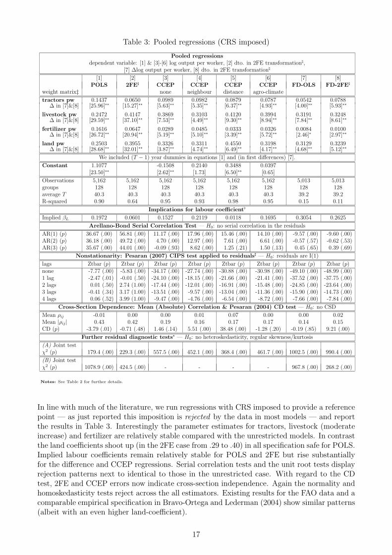
Table 3: Pooled regressions (CRS imposed)
Pooled regressionsdependent variable: [1] & [3]-[6] log output per worker, [2] dto. in 2FE transformation\,
[7] ∆log output per worker, [8] dto. in 2FE transformation\
[1] [2] [3] [4] [5] [6] [7] [8]POLS 2FE\ CCEP CCEP CCEP CCEP FD-OLS FD-2FE\
weight matrix‡ none neighbour distance agro-climate
tractors pw 0.1437 0.0650 0.0989 0.0982 0.0879 0.0787 0.0542 0.0788∆ in [7]&[8] [25.96]∗∗ [15.27]∗∗ [5.63]∗∗ [5.35]∗∗ [6.37]∗∗ [4.93]∗∗ [4.00]∗∗ [5.93]∗∗
livestock pw 0.2472 0.4147 0.3869 0.3103 0.4120 0.3994 0.3191 0.3248∆ in [7]&[8] [29.59]∗∗ [37.10]∗∗ [7.53]∗∗ [4.49]∗∗ [9.30]∗∗ [8.94]∗∗ [7.84]∗∗ [8.61]∗∗
fertilizer pw 0.1616 0.0647 0.0289 0.0485 0.0333 0.0326 0.0084 0.0100∆ in [7]&[8] [26.72]∗∗ [20.94]∗∗ [5.19]∗∗ [5.10]∗∗ [3.39]∗∗ [5.72]∗∗ [2.46]∗ [2.97]∗∗
land pw 0.2503 0.3955 0.3326 0.3311 0.4550 0.3198 0.3129 0.3239∆ in [7]&[8] [28.68]∗∗ [32.01]∗∗ [3.87]∗∗ [4.74]∗∗ [6.49]∗∗ [4.17]∗∗ [4.68]∗∗ [5.12]∗∗
We included (T − 1) year dummies in equations [1] and (in first differences) [7].
Constant 1.1077 -0.1508 0.2140 0.3488 0.0397[23.50]∗∗ [2.62]∗∗ [1.73] [6.50]∗∗ [0.65]
Observations 5,162 5,162 5,162 5,162 5,162 5,162 5,013 5,013groups 128 128 128 128 128 128 128 128average T 40.3 40.3 40.3 40.3 40.3 40.3 39.2 39.2R-squared 0.90 0.64 0.95 0.93 0.98 0.95 0.15 0.11
Implications for labour coefficient[
Implied βL 0.1972 0.0601 0.1527 0.2119 0.0118 0.1695 0.3054 0.2625
Arellano-Bond Serial Correlation Test — H0: no serial correlation in the residuals
AR(1) (p) 36.67 (.00) 56.81 (.00) 11.17 (.00) 17.96 (.00) 15.46 (.00) 14.10 (.00) -9.57 (.00) -9.60 (.00)AR(2) (p) 36.18 (.00) 49.72 (.00) 4.70 (.00) 12.97 (.00) 7.61 (.00) 6.61 (.00) -0.57 (.57) -0.62 (.53)AR(3) (p) 35.67 (.00) 44.01 (.00) -0.09 (.93) 8.62 (.00) 1.25 (.21) 1.50 (.13) 0.45 (.65) 0.39 (.69)
Nonstationarity: Pesaran (2007) CIPS test applied to residuals] — H0: residuals are I(1)
lags Ztbar (p) Ztbar (p) Ztbar (p) Ztbar (p) Ztbar (p) Ztbar (p) Ztbar (p) Ztbar (p)none -7.77 (.00) -5.83 (.00) -34.17 (.00) -27.74 (.00) -30.88 (.00) -30.98 (.00) -49.10 (.00) -48.99 (.00)1 lag -2.47 (.01) -0.01 (.50) -24.10 (.00) -18.15 (.00) -21.66 (.00) -21.41 (.00) -37.52 (.00) -37.75 (.00)2 lags 0.01 (.50) 2.74 (1.00) -17.44 (.00) -12.01 (.00) -16.91 (.00) -15.48 (.00) -24.85 (.00) -23.64 (.00)3 lags -0.41 (.34) 3.17 (1.00) -13.51 (.00) -9.57 (.00) -13.04 (.00) -11.36 (.00) -15.90 (.00) -14.73 (.00)4 lags 0.06 (.52) 3.99 (1.00) -9.47 (.00) -4.76 (.00) -6.54 (.00) -8.72 (.00) -7.66 (.00) -7.84 (.00)
Cross-Section Dependence: Mean (Absolute) Correlation & Pesaran (2004) CD test — H0: no CSD
Mean ρij -0.01 0.00 0.00 0.01 0.07 0.00 0.00 0.02Mean |ρij| 0.43 0.42 0.19 0.16 0.17 0.17 0.14 0.15CD (p) -3.79 (.01) -0.71 (.48) 1.46 (.14) 5.51 (.00) 38.48 (.00) -1.28 (.20) -0.19 (.85) 9.21 (.00)
Further residual diagnostic tests? — H0: no heteroskedasticity, regular skewness/kurtosis
(A) Joint testχ2 (p) 179.4 (.00) 229.3 (.00) 557.5 (.00) 452.1 (.00) 368.4 (.00) 461.7 (.00) 1002.5 (.00) 990.4 (.00)
(B) Joint testχ2 (p) 1078.9 (.00) 424.5 (.00) - - - - 967.8 (.00) 268.2 (.00)
Notes: See Table 2 for further details.
In line with much of the literature, we run regressions with CRS imposed to provide a referencepoint — as just reported this imposition is rejected by the data in most models — and reportthe results in Table 3. Interestingly the parameter estimates for tractors, livestock (moderateincrease) and fertilizer are relatively stable compared with the unrestricted models. In contrastthe land coefficients shoot up (in the 2FE case from .29 to .40) in all specification safe for POLS.Implied labour coefficients remain relatively stable for POLS and 2FE but rise substantiallyfor the difference and CCEP regressions. Serial correlation tests and the unit root tests displayrejection patterns next to identical to those in the unrestricted case. With regard to the CDtest, 2FE and CCEP errors now indicate cross-section independence. Again the normality andhomoskedasticity tests reject across the all estimators. Existing results for the FAO data and acomparable empirical specification in Bravo-Ortega and Lederman (2004) show similar patterns(albeit with an even higher land-coefficient).
17
We can see from these results that the the erroneous imposition of CRS (the unrestricted modelsreject CRS) has led to larger magnitudes for either the land or the implied labour coefficient —in the commonly preferred 2FE model the implied labour coefficient has merely risen from .03 to.06 — albeit with diagnostics that reject the most common regression assumptions for this esti-mator (residuals which are stationary, serially uncorrelated, normal and homoskedastic). Notethat our empirical setup implies that factor-input parameters are unidentified in the POLS and2FE if the same unobserved common factors drive output and inputs.
Regarding the Pesaran (2006) CCEP and our extensions, our results show that the former em-phatically rejects CRS and yields summed input elasticities of around .68, with negative impliedlabour coefficient; of the other CCE estimators the distance version behaves in a similar fash-ion, whereas the other two cannot reject CRS. Serial correlation remains a concern in all fourmodels. Surprisingly the agro-climate version is the only model that cannot reject cross-sectionindependence. Once CRS is (despite previous results) imposed, all models yield somewhatsimilar coefficients, with the land coefficient again rising considerably — most obviously so inthe distance model. Diagnostics remain similar, although residuals in the standard CCEP nowcannot reject cross-sectional independence.
In conclusion, our pooled models largely reject constant returns to scale, yield very low values forthe implied coefficient on labour and over a range of specification tests indicate a combination ofnon-normality and heteroskedasticity, cross-section dependence, nonstationarity and/or serialcorrelation in the residuals. Allowing for heterogeneity in the unobserved common factors(CCEP) although alleviating a potential identification problem does not seem to provide anoverall panacea; in fact for the most part the CCEP-type estimators are suggested to continuesuffering from cross-section dependence. Our next analytical step is therefore to investigate howthe parameter estimates and diagnostic tests change if we allow for technology heterogeneityacross countries.
4.3 Averaged country regression estimates
We present the results from Mean-Group type estimators in the unrestricted regression model(CRS not imposed) in Table 4. For all estimators we present the mean and robust mean acrossN country parameters — the latter uses weights to reduce the impact of outliers. In practicethe median estimates (not reported) are very close to the robust estimates. In our discussionbelow we focus on the robust means. The t-statistics reported for each average estimate testwhether the average parameter is statistically different from zero, following Pesaran, Smith,and Yamagata (2008).
The MG, as well as our two Augmented Mean Group estimators display large decreasing re-turns, although in the AMG version (i) only at the 10% level of significance. The standard,neighbour and agro-climate CCEMG in contrast have insignificant coefficients on labour, in-dicating constant returns in the average country regression. Around 30 to 40 countries rejectCRS at 5% level of significance in each of these models. The distance CCEMG indicates verylarge and highly significant decreasing returns to scale.
Regarding average parameter estimates on the factor inputs, the MG and AMG estimatorsyield next to identical results: capital around .07, livestock around .25, fertilizer around .03
18
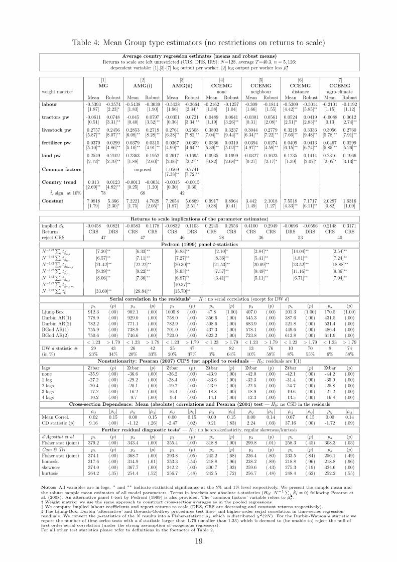
Table 4: Mean Group type estimators (no restrictions on returns to scale)
Average country regression estimates (means and robust means)Returns to scale are left unrestricted (CRS, DRS, IRS); N=128, average T=40.3, n = 5, 126;
dependent variable: [1],[3]-[7] log output per worker, [2] log output per worker less µ•t
[1] [2] [3] [4] [5] [6] [7]MG AMG(i) AMG(ii) CCEMG CCEMG CCEMG CCEMG
weight matrix† none neighbour distance agro-climateMean Robust Mean Robust Mean Robust Mean Robust Mean Robust Mean Robust Mean Robust
labour -0.5393 -0.3574 -0.5438 -0.3039 -0.5438 -0.3664 -0.2162 -0.1257 -0.309 -0.1814 -0.5309 -0.5014 -0.2101 -0.1192[1.87] [2.23]∗ [1.83] [1.90] [1.96] [2.34]∗ [1.38] [1.04] [1.66] [1.55] [4.42]∗∗ [5.85]∗∗ [1.15] [1.12]
tractors pw -0.0611 0.0748 -0.045 0.0797 -0.0351 0.0721 0.0489 0.0641 -0.0301 0.0561 0.0524 0.0419 -0.0088 0.0612[0.51] [3.31]∗∗ [0.40] [3.52]∗∗ [0.36] [3.34]∗∗ [1.19] [3.26]∗∗ [0.31] [2.08]∗ [2.51]* [2.83]∗∗ [0.13] [2.74]∗∗
livestock pw 0.2757 0.2456 0.2853 0.2719 0.2761 0.2508 0.3803 0.3237 0.3044 0.2779 0.3219 0.3336 0.3056 0.2760[5.87]∗∗ [8.07]∗∗ [6.08]∗∗ [8.28]∗∗ [6.38]∗∗ [7.82]∗∗ [7.04]∗∗ [9.44]∗∗ [6.34]∗∗ [7.22]∗∗ [7.66]∗∗ [9.48]∗∗ [5.78]∗∗ [7.91]∗∗
fertilizer pw 0.0370 0.0299 0.0379 0.0315 0.0367 0.0309 0.0366 0.0310 0.0394 0.0274 0.0409 0.0413 0.0467 0.0299[5.10]∗∗ [4.86]∗∗ [5.10]∗∗ [4.91]∗∗ [4.99]∗∗ [4.64]∗∗ [5.39]∗∗ [5.02]∗∗ [4.97]∗∗ [4.59]∗∗ [6.15]∗∗ [6.74]∗∗ [5.85]∗∗ [5.26]∗∗
land pw 0.2549 0.2102 0.2363 0.1952 0.2617 0.1695 0.0935 0.1999 -0.0327 0.1623 0.1235 0.1414 0.2316 0.1966[2.12]∗ [2.79]∗∗ [1.88] [2.60]∗ [2.06]∗ [2.27]∗ [0.82] [2.68]∗∗ [0.27] [2.17]∗ [1.39] [2.07]∗ [2.05]∗ [3.13]∗∗
Common factors imposed 1.0569 0.7741[7.38]∗∗ [7.72]∗∗
Country trend 0.013 0.0123 -0.0013 -0.0031 -0.0015 -0.0015[2.69]∗∗ [4.82]∗∗ [0.25] [1.20] [0.30] [0.30]
ti sign. at 10% 78 68 42
Constant 7.0818 5.366 7.2221 4.7029 7.2654 5.6869 0.9917 0.8964 3.442 2.1018 7.5518 7.1717 2.0287 1.6316[1.79] [2.30]∗ [1.75] [2.05]∗ [1.87] [2.51]∗ [0.38] [0.41] [1.49] [1.27] [4.33]∗∗ [6.11]∗∗ [0.82] [1.09]
Returns to scale implications of the parameter estimates‡implied βL -0.0458 0.0821 -0.0583 0.1178 -0.0832 0.1103 0.2245 0.2556 0.4100 0.2949 -0.0696 -0.0596 0.2148 0.3171Returns CRS DRS CRS CRS CRS DRS CRS CRS CRS CRS DRS DRS CRS CRSreject CRS 47 47 46 28 36 53 40
Pedroni (1999) panel t-statistics
N−1/2∑
i tβL,i [7.20]∗∗ [6.33]∗∗ [6.83]∗∗ [2.10]∗ [2.84]∗∗ [14.04]∗∗ [2.54]∗∗
N−1/2∑
i tβtr,i [6.57]∗∗ [7.11]∗∗ [7.27]∗∗ [8.36]∗∗ [5.41]∗∗ [4.81]∗∗ [7.24]∗∗
N−1/2∑
i tβlive,i [21.42]∗∗ [22.22]∗∗ [20.30]∗∗ [21.53]∗∗ [20.09]∗∗ [23.52]∗∗ [18.88]∗∗
N−1/2∑
i tβf,i [9.39]∗∗ [9.22]∗∗ [8.93]∗∗ [7.57]∗∗ [9.49]∗∗ [11.16]∗∗ [9.36]∗∗
N−1/2∑
i tβn,i [8.06]∗∗ [7.36]∗∗ [6.87]∗∗ [3.41]∗∗ [5.11]∗∗ [6.71]∗∗ [7.04]∗∗
N−1/2∑
i tβTFP,i [10.37]∗∗
N−1/2∑
i tti [33.60]∗∗ [28.84]∗∗ [15.70]∗∗
Serial correlation in the residuals] — H0: no serial correlation (except for DW d)
pλ (p) pλ (p) pλ (p) pλ (p) pλ (p) pλ (p) pλ (p)Ljung-Box 912.3 (.00) 902.1 (.00) 1005.8 (.00) 47.8 (1.00) 407.0 (.00) 201.3 (1.00) 170.5 (1.00)Durbin AR(1) 778.9 (.00) 929.0 (.00) 758.0 (.00) 356.6 (.00) 545.3 (.00) 387.6 (.00) 431.5 (.00)Durbin AR(2) 782.2 (.00) 771.1 (.00) 782.9 (.00) 508.6 (.00) 683.9 (.00) 521.8 (.00) 531.4 (.00)BGod AR(1) 755.9 (.00) 738.9 (.00) 701.0 (.00) 437.3 (.00) 578.1 (.00) 449.6 (.00) 486.4 (.00)BGod AR(2) 750.6 (.00) 746.6 (.00) 720.0 (.00) 623.2 (.00) 723.8 (.00) 613.8 (.00) 611.9 (.00)
< 1.23 > 1.79 < 1.23 > 1.79 < 1.23 > 1.79 < 1.23 > 1.79 < 1.23 > 1.79 < 1.23 > 1.79 < 1.23 > 1.79DW d statistic # 29 43 26 42 25 47 4 82 13 76 10 70 8 74(in %) 23% 34% 20% 33% 20% 37% 3% 64% 10% 59% 8% 55% 6% 58%
Nonstationarity: Pesaran (2007) CIPS test applied to residuals — H0: residuals are I(1)
lags Ztbar (p) Ztbar (p) Ztbar (p) Ztbar (p) Ztbar (p) Ztbar (p) Ztbar (p)none -35.9 (.00) -36.6 (.00) -36.2 (.00) -43.9 (.00) -42.0 (.00) -42.1 (.00) -44.2 (.00)1 lag -27.2 (.00) -29.2 (.00) -28.4 (.00) -33.6 (.00) -32.3 (.00) -31.4 (.00) -35.0 (.00)2 lags -20.4 (.00) -20.1 (.00) -19.7 (.00) -23.9 (.00) -22.5 (.00) -24.7 (.00) -25.8 (.00)3 lags -17.2 (.00) -16.2 (.00) -16.4 (.00) -18.8 (.00) -18.9 (.00) -19.6 (.00) -21.2 (.00)4 lags -10.2 (.00) -9.7 (.00) -9.4 (.00) -14.1 (.00) -12.3 (.00) -13.5 (.00) -16.8 (.00)
Cross-section Dependence: Mean (absolute) correlations and Pesaran (2004) test — H0: no CSD in the residuals
ρij |ρij| ρij |ρij| ρij |ρij| ρij |ρij| ρij |ρij| ρij |ρij| ρij |ρij|Mean Correl. 0.02 0.15 0.00 0.15 0.00 0.15 0.00 0.15 0.00 0.14 0.07 0.15 0.00 0.14CD statistic (p) 9.16 (.00) -1.12 (.26) -2.47 (.02) 0.21 (.83) 2.24 (.03) 37.16 (.00) -1.72 (.09)
Further residual diagnostic tests? — H0: no heteroskedasticity, regular skewness/kurtosis
d’Agostini et al pλ (p) pλ (p) pλ (p) pλ (p) pλ (p) pλ (p) pλ (p)Fisher stat (joint) 379.2 (.00) 343.4 (.00) 355.4 (.00) 318.8 (.00) 299.8 (.01) 258.3 (.45) 308.3 (.03)
Cam & Tri pλ (p) pλ (p) pλ (p) pλ (p) pλ (p) pλ (p) pλ (p)Fisher stat (joint) 374.1 (.00) 368.7 (.00) 293.8 (.05) 245.2 (.68) 236.4 (.80) 233.5 (.84) 256.1 (.49)homosk. 317.6 (.00) 314.9 (.01) 253.3 (.54) 218.8 (.96) 228.2 (.89) 218.8 (.96) 218.8 (.96)skewness 374.0 (.00) 367.7 (.00) 342.2 (.00) 300.7 (.03) 259.6 (.43) 275.3 (.19) 324.6 (.00)kurtosis 264.2 (.35) 254.4 (.52) 256.7 (.48) 242.5 (.72) 256.7 (.48) 248.4 (.62) 252.2 (.55)
Notes: All variables are in logs. ∗ and ∗∗ indicate statistical significance at the 5% and 1% level respectively. We present the sample mean and
the robust sample mean estimates of all model parameters. Terms in brackets are absolute t-statistics (H0: N−1∑i βi = 0) following Pesaran et
al. (2008). An alternative panel t-test by Pedroni (1999) is also provided. The ‘common factors’ variable refers to µ•t .† Weight matrix: we use the same approach to construct cross-section averages as in the pooled regressions.‡ We compute implied labour coefficients and report returns to scale (DRS, CRS are decreasing and constant returns respectively).] The Ljung-Box, Durbin ‘alternative’ and Breusch-Godfrey procedures test first- and higher-order serial correlation in time-series regressionresiduals. We convert the p-statistics of the N results into a Fisher-statistic pλ which is distributed χ2(2N). For the Durbin-Watson d statistic wereport the number of time-series tests with a d statistic larger than 1.79 (smaller than 1.23) which is deemed to (be unable to) reject the null offirst order serial correlation (under the strong assumption of exogenous regressors).For all other test statistics please refer to definitions in the footnotes of Table 2.
19
and land around .20. In comparison to the parameter differences across models in the pooledspecifications, the MG and AMG parameter estimates are relatively similar to those in theCCEMG models, with the crucial exception of the returns to scale coefficient and thus theimplied labour elasticity: in the former group of models the labour coefficient is around .10,whereas in the latter group it is closer to .30 (leaving the nonsensical results produced by thedistance CCEMG to one side). Within the CCEMG group the standard and the agro-climateestimators yield very similar results.
Turning to the diagnostics, all models reject nonstationary errors in the Pesaran (2007) CIPStest. The panel t-statistic following Pedroni (1999) suggests that all coefficients are significantat the 5% level, in contrast to the t-statistic following Pesaran et al. (2008) which we used forour discussion above. Mean absolute error correlation is uniformly low at .15 for all estimators,but cross-section independence is rejected in the MG and AMG(ii), as well as in the alternativeCCEMG estimators (marginally in case of the agro-climate CCEMG). For the serial correlationtests we need to take recourse to statistics constructed from country-regression diagnostics. Ineach case these are Fisher (1932)-type statistics (labelled pλ), derived from p-values for thetest statistics in each country.12 As can be seen the Durbin ‘alternative’ and Breusch-Godfreyprocedures reject the absence of serially correlated errors, whereas for the Ljung-Watson andDurbin-Watson statistics (see table footnotes) there is some evidence for serially uncorrelatederrors in the CCEMG-type estimators. Furthermore, the error normality and homoskedasticitytests (similarly expressed as Fisher-statistics) suggest these properties are rejected in the MGand AMG estimators, and offer conflicting evidence across the CCEMG-type models.
Taking the results for all diagnostic tests into account and recognising the potential problemsof the use of time-series tests adjusted for the panel context via computation of the Fisher(1932) statistic, we suggest that evidence in favour of the standard CCEMG and agro-climateCCEMG seems most convincing: compared to the other models these provide some evidenceof serially uncorrelated and normal residuals. Since neither of these estimators can reject CRSfor the average country production function, we rerun all heterogeneous parameter models withCRS imposed.
The CRS country regression averages in Table 5 produce very similar results across all estima-tors: it can be seen that the imposition of CRS in heterogeneous regression models does notcreate the same dramatic changes to the estimates as in the pooled estimator case. It can alsobe seen that the individual country-estimates for each model now contain less outliers, as isevidenced by the precision of the mean estimates and their proximity in parameter value to therobust mean estimates. We focus on the models for which on average we had not rejected CRS:AMG(i), standard, neighbour and agro-climate CCEMG. Factor elasticities in the AMG(i) areclose to the unrestricted model ones, with the obvious exception of implied labour, which withCRS imposed is around .33 rather than .12. The standard and agro-climate CCEMG nowmatch each other’s (robust) mean parameters even closer than in the unrestricted case, whilethe neighbour CCEMG in comparison has an inflated land coefficient. Panel t-statistics aresignificant at the 1% level for all parameters in all models and CIPS tests continue to reject non-stationarity in the residuals. AMG(i) as well as standard and agro-climate CCEMG residualsappear cross-sectionally independent.
12Constructed as pλ = −2∑i log(pi), distribution χ2(2N).
20
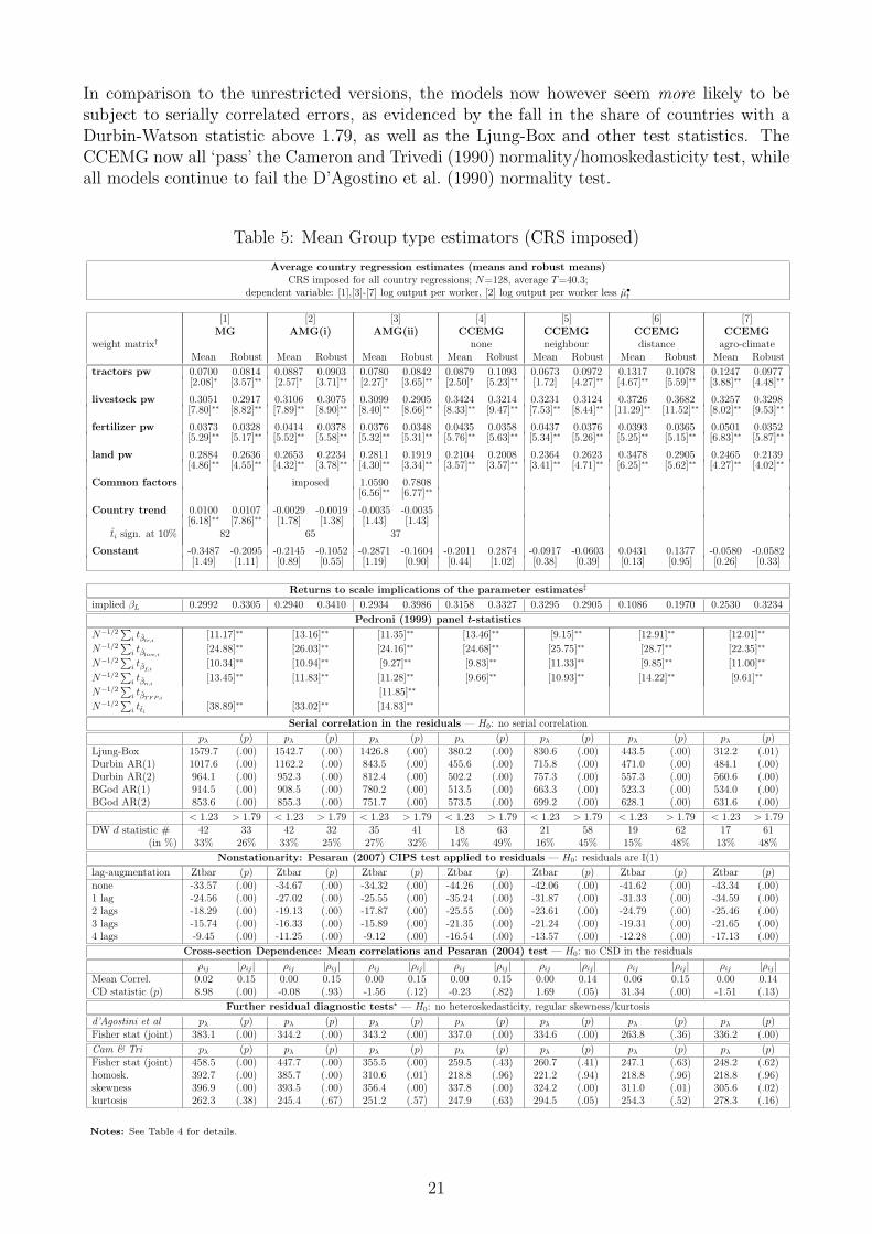
In comparison to the unrestricted versions, the models now however seem more likely to besubject to serially correlated errors, as evidenced by the fall in the share of countries with aDurbin-Watson statistic above 1.79, as well as the Ljung-Box and other test statistics. TheCCEMG now all ‘pass’ the Cameron and Trivedi (1990) normality/homoskedasticity test, whileall models continue to fail the D’Agostino et al. (1990) normality test.
Table 5: Mean Group type estimators (CRS imposed)
Average country regression estimates (means and robust means)CRS imposed for all country regressions; N=128, average T=40.3;
dependent variable: [1],[3]-[7] log output per worker, [2] log output per worker less µ•t
[1] [2] [3] [4] [5] [6] [7]MG AMG(i) AMG(ii) CCEMG CCEMG CCEMG CCEMG
weight matrix† none neighbour distance agro-climateMean Robust Mean Robust Mean Robust Mean Robust Mean Robust Mean Robust Mean Robust
tractors pw 0.0700 0.0814 0.0887 0.0903 0.0780 0.0842 0.0879 0.1093 0.0673 0.0972 0.1317 0.1078 0.1247 0.0977[2.08]∗ [3.57]∗∗ [2.57]∗ [3.71]∗∗ [2.27]∗ [3.65]∗∗ [2.50]∗ [5.23]∗∗ [1.72] [4.27]∗∗ [4.67]∗∗ [5.59]∗∗ [3.88]∗∗ [4.48]∗∗
livestock pw 0.3051 0.2917 0.3106 0.3075 0.3099 0.2905 0.3424 0.3214 0.3231 0.3124 0.3726 0.3682 0.3257 0.3298[7.80]∗∗ [8.82]∗∗ [7.89]∗∗ [8.90]∗∗ [8.40]∗∗ [8.66]∗∗ [8.33]∗∗ [9.47]∗∗ [7.53]∗∗ [8.44]∗∗ [11.29]∗∗ [11.52]∗∗ [8.02]∗∗ [9.53]∗∗
fertilizer pw 0.0373 0.0328 0.0414 0.0378 0.0376 0.0348 0.0435 0.0358 0.0437 0.0376 0.0393 0.0365 0.0501 0.0352[5.29]∗∗ [5.17]∗∗ [5.52]∗∗ [5.58]∗∗ [5.32]∗∗ [5.31]∗∗ [5.76]∗∗ [5.63]∗∗ [5.34]∗∗ [5.26]∗∗ [5.25]∗∗ [5.15]∗∗ [6.83]∗∗ [5.87]∗∗
land pw 0.2884 0.2636 0.2653 0.2234 0.2811 0.1919 0.2104 0.2008 0.2364 0.2623 0.3478 0.2905 0.2465 0.2139[4.86]∗∗ [4.55]∗∗ [4.32]∗∗ [3.78]∗∗ [4.30]∗∗ [3.34]∗∗ [3.57]∗∗ [3.57]∗∗ [3.41]∗∗ [4.71]∗∗ [6.25]∗∗ [5.62]∗∗ [4.27]∗∗ [4.02]∗∗
Common factors imposed 1.0590 0.7808[6.56]∗∗ [6.77]∗∗
Country trend 0.0100 0.0107 -0.0029 -0.0019 -0.0035 -0.0035[6.18]∗∗ [7.86]∗∗ [1.78] [1.38] [1.43] [1.43]
ti sign. at 10% 82 65 37
Constant -0.3487 -0.2095 -0.2145 -0.1052 -0.2871 -0.1604 -0.2011 0.2874 -0.0917 -0.0603 0.0431 0.1377 -0.0580 -0.0582[1.49] [1.11] [0.89] [0.55] [1.19] [0.90] [0.44] [1.02] [0.38] [0.39] [0.13] [0.95] [0.26] [0.33]
Returns to scale implications of the parameter estimates‡
implied βL 0.2992 0.3305 0.2940 0.3410 0.2934 0.3986 0.3158 0.3327 0.3295 0.2905 0.1086 0.1970 0.2530 0.3234
Pedroni (1999) panel t-statistics
N−1/2∑
i tβtr,i [11.17]∗∗ [13.16]∗∗ [11.35]∗∗ [13.46]∗∗ [9.15]∗∗ [12.91]∗∗ [12.01]∗∗
N−1/2∑
i tβlive,i [24.88]∗∗ [26.03]∗∗ [24.16]∗∗ [24.68]∗∗ [25.75]∗∗ [28.7]∗∗ [22.35]∗∗
N−1/2∑
i tβf,i [10.34]∗∗ [10.94]∗∗ [9.27]∗∗ [9.83]∗∗ [11.33]∗∗ [9.85]∗∗ [11.00]∗∗
N−1/2∑
i tβn,i [13.45]∗∗ [11.83]∗∗ [11.28]∗∗ [9.66]∗∗ [10.93]∗∗ [14.22]∗∗ [9.61]∗∗
N−1/2∑
i tβTFP,i [11.85]∗∗
N−1/2∑
i tti [38.89]∗∗ [33.02]∗∗ [14.83]∗∗
Serial correlation in the residuals — H0: no serial correlation
pλ (p) pλ (p) pλ (p) pλ (p) pλ (p) pλ (p) pλ (p)Ljung-Box 1579.7 (.00) 1542.7 (.00) 1426.8 (.00) 380.2 (.00) 830.6 (.00) 443.5 (.00) 312.2 (.01)Durbin AR(1) 1017.6 (.00) 1162.2 (.00) 843.5 (.00) 455.6 (.00) 715.8 (.00) 471.0 (.00) 484.1 (.00)Durbin AR(2) 964.1 (.00) 952.3 (.00) 812.4 (.00) 502.2 (.00) 757.3 (.00) 557.3 (.00) 560.6 (.00)BGod AR(1) 914.5 (.00) 908.5 (.00) 780.2 (.00) 513.5 (.00) 663.3 (.00) 523.3 (.00) 534.0 (.00)BGod AR(2) 853.6 (.00) 855.3 (.00) 751.7 (.00) 573.5 (.00) 699.2 (.00) 628.1 (.00) 631.6 (.00)
< 1.23 > 1.79 < 1.23 > 1.79 < 1.23 > 1.79 < 1.23 > 1.79 < 1.23 > 1.79 < 1.23 > 1.79 < 1.23 > 1.79DW d statistic # 42 33 42 32 35 41 18 63 21 58 19 62 17 61
(in %) 33% 26% 33% 25% 27% 32% 14% 49% 16% 45% 15% 48% 13% 48%
Nonstationarity: Pesaran (2007) CIPS test applied to residuals — H0: residuals are I(1)
lag-augmentation Ztbar (p) Ztbar (p) Ztbar (p) Ztbar (p) Ztbar (p) Ztbar (p) Ztbar (p)none -33.57 (.00) -34.67 (.00) -34.32 (.00) -44.26 (.00) -42.06 (.00) -41.62 (.00) -43.34 (.00)1 lag -24.56 (.00) -27.02 (.00) -25.55 (.00) -35.24 (.00) -31.87 (.00) -31.33 (.00) -34.59 (.00)2 lags -18.29 (.00) -19.13 (.00) -17.87 (.00) -25.55 (.00) -23.61 (.00) -24.79 (.00) -25.46 (.00)3 lags -15.74 (.00) -16.33 (.00) -15.89 (.00) -21.35 (.00) -21.24 (.00) -19.31 (.00) -21.65 (.00)4 lags -9.45 (.00) -11.25 (.00) -9.12 (.00) -16.54 (.00) -13.57 (.00) -12.28 (.00) -17.13 (.00)
Cross-section Dependence: Mean correlations and Pesaran (2004) test — H0: no CSD in the residuals
ρij |ρij| ρij |ρij| ρij |ρij| ρij |ρij| ρij |ρij| ρij |ρij| ρij |ρij|Mean Correl. 0.02 0.15 0.00 0.15 0.00 0.15 0.00 0.15 0.00 0.14 0.06 0.15 0.00 0.14CD statistic (p) 8.98 (.00) -0.08 (.93) -1.56 (.12) -0.23 (.82) 1.69 (.05) 31.34 (.00) -1.51 (.13)
Further residual diagnostic tests? — H0: no heteroskedasticity, regular skewness/kurtosis
d’Agostini et al pλ (p) pλ (p) pλ (p) pλ (p) pλ (p) pλ (p) pλ (p)Fisher stat (joint) 383.1 (.00) 344.2 (.00) 343.2 (.00) 337.0 (.00) 334.6 (.00) 263.8 (.36) 336.2 (.00)
Cam & Tri pλ (p) pλ (p) pλ (p) pλ (p) pλ (p) pλ (p) pλ (p)Fisher stat (joint) 458.5 (.00) 447.7 (.00) 355.5 (.00) 259.5 (.43) 260.7 (.41) 247.1 (.63) 248.2 (.62)homosk. 392.7 (.00) 385.7 (.00) 310.6 (.01) 218.8 (.96) 221.2 (.94) 218.8 (.96) 218.8 (.96)skewness 396.9 (.00) 393.5 (.00) 356.4 (.00) 337.8 (.00) 324.2 (.00) 311.0 (.01) 305.6 (.02)kurtosis 262.3 (.38) 245.4 (.67) 251.2 (.57) 247.9 (.63) 294.5 (.05) 254.3 (.52) 278.3 (.16)
Notes: See Table 4 for details.
21
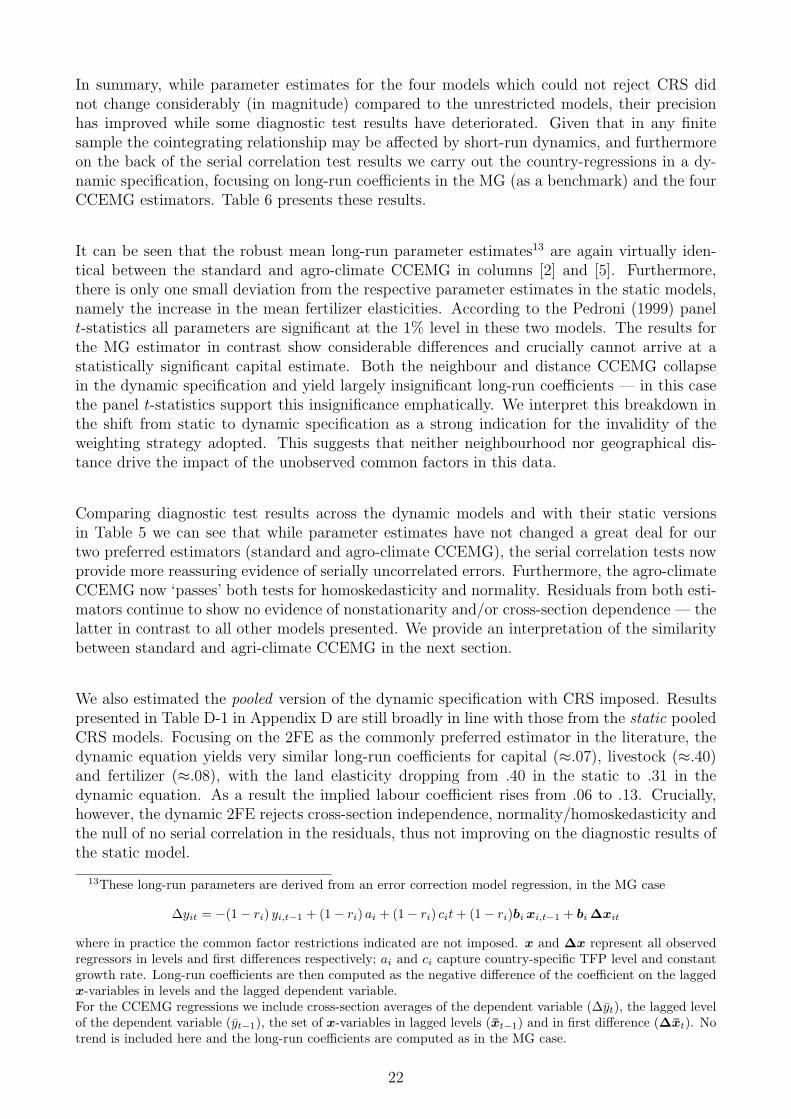
In summary, while parameter estimates for the four models which could not reject CRS didnot change considerably (in magnitude) compared to the unrestricted models, their precisionhas improved while some diagnostic test results have deteriorated. Given that in any finitesample the cointegrating relationship may be affected by short-run dynamics, and furthermoreon the back of the serial correlation test results we carry out the country-regressions in a dy-namic specification, focusing on long-run coefficients in the MG (as a benchmark) and the fourCCEMG estimators. Table 6 presents these results.
It can be seen that the robust mean long-run parameter estimates13 are again virtually iden-tical between the standard and agro-climate CCEMG in columns [2] and [5]. Furthermore,there is only one small deviation from the respective parameter estimates in the static models,namely the increase in the mean fertilizer elasticities. According to the Pedroni (1999) panelt-statistics all parameters are significant at the 1% level in these two models. The results forthe MG estimator in contrast show considerable differences and crucially cannot arrive at astatistically significant capital estimate. Both the neighbour and distance CCEMG collapsein the dynamic specification and yield largely insignificant long-run coefficients — in this casethe panel t-statistics support this insignificance emphatically. We interpret this breakdown inthe shift from static to dynamic specification as a strong indication for the invalidity of theweighting strategy adopted. This suggests that neither neighbourhood nor geographical dis-tance drive the impact of the unobserved common factors in this data.
Comparing diagnostic test results across the dynamic models and with their static versionsin Table 5 we can see that while parameter estimates have not changed a great deal for ourtwo preferred estimators (standard and agro-climate CCEMG), the serial correlation tests nowprovide more reassuring evidence of serially uncorrelated errors. Furthermore, the agro-climateCCEMG now ‘passes’ both tests for homoskedasticity and normality. Residuals from both esti-mators continue to show no evidence of nonstationarity and/or cross-section dependence — thelatter in contrast to all other models presented. We provide an interpretation of the similaritybetween standard and agri-climate CCEMG in the next section.
We also estimated the pooled version of the dynamic specification with CRS imposed. Resultspresented in Table D-1 in Appendix D are still broadly in line with those from the static pooledCRS models. Focusing on the 2FE as the commonly preferred estimator in the literature, thedynamic equation yields very similar long-run coefficients for capital (≈.07), livestock (≈.40)and fertilizer (≈.08), with the land elasticity dropping from .40 in the static to .31 in thedynamic equation. As a result the implied labour coefficient rises from .06 to .13. Crucially,however, the dynamic 2FE rejects cross-section independence, normality/homoskedasticity andthe null of no serial correlation in the residuals, thus not improving on the diagnostic results ofthe static model.
13These long-run parameters are derived from an error correction model regression, in the MG case
∆yit = −(1− ri) yi,t−1 + (1− ri) ai + (1− ri) cit+ (1− ri)bi xi,t−1 + bi ∆xit
where in practice the common factor restrictions indicated are not imposed. x and ∆x represent all observedregressors in levels and first differences respectively; ai and ci capture country-specific TFP level and constantgrowth rate. Long-run coefficients are then computed as the negative difference of the coefficient on the laggedx-variables in levels and the lagged dependent variable.For the CCEMG regressions we include cross-section averages of the dependent variable (∆yt), the lagged levelof the dependent variable (yt−1), the set of x-variables in lagged levels (xt−1) and in first difference (∆xt). Notrend is included here and the long-run coefficients are computed as in the MG case.
22
Table 6: Dynamic Specification — MG-type estimators (CRS imposed)
Average country long-run coefficient estimates (means and robust means)CRS imposed for all country regressions; N=128, average T=39.2;
dependent variable: growth of output per worker
[1] [2] [3] [4] [5]MG CCEMG CCEMG CCEMG CCEMG
weight matrix† none neighbour distance agro-climateMean Robust Mean Robust Mean Robust Mean Robust Mean Robust
long-run coefficientstractors pw 0.346 0.043 0.099 0.088 0.125 0.019 -2.780 -0.116 0.121 0.085
[1.19] [1.50] [1.37] [3.18]∗∗ [0.24] [0.14] [0.78] [1.39] [1.67] [2.85]∗∗
livestock pw 0.405 0.288 0.304 0.307 1.203 -0.381 -5.298 -0.597 0.316 0.327[3.33]∗∗ [6.97]∗∗ [3.71]∗∗ [6.82]∗∗ [0.51] [1.75] [1.66] [3.43]∗∗ [3.46]∗∗ [6.67]∗∗
fertilizer pw 0.123 0.046 0.070 0.054 0.576 -0.016 -0.546 -0.015 0.081 0.077[1.67] [4.50]∗∗ [5.41]∗∗ [4.84]∗∗ [0.86] [0.39] [0.84] [0.48] [6.59]∗∗ [6.42]∗∗
land pw -4.940 0.188 0.244 0.215 0.623 -0.055 -3.026 0.007 0.102 0.191[0.95] [2.50]∗ [2.42]∗ [2.73]∗∗ [0.49] [0.23] [0.64] [0.03] [0.72] [2.33]∗
trend 0.007 0.006[4.00]∗∗ [4.96]∗∗
ti sign. at 10% 58
Constant -0.476 -0.098 -1.242 0.056 -0.053 0.061 0.151 0.002 0.030 0.020[1.76] [0.71] [2.00]∗ [0.16] [0.15] [0.34] [0.65] [0.01] [0.09] [0.10]
Returns to scale implications of the parameter estimates‡
implied βL 5.066 0.436 0.284 0.335 -1.526 1.433 12.649 1.721 0.381 0.321
Serial correlation in the residuals — H0: no serial correlation
pλ (p) pλ (p) pλ (p) pλ (p) pλ (p)Ljung-Box 72.9 (1.00) 0.6 (1.00) 21.0 (1.00) 2.1 (1.00) 0.9 (1.00)Durbin AR(1) 299.3 (.03) 332.4 (.00) 487.5 (.00) 488.3 (.00) 493.2 (.00)Durbin AR(2) 370.5 (.00) 525.8 (.00) 678.2 (.00) 741.9 (.00) 775.2 (.00)BGod AR(1) 366.7 (.00) 573.0 (.00) 781.9 (.00) 715.4 (.00) 775.2 (.00)BGod AR(2) 465.6 (.00) 902.7 (.00) 1072.3 (.00) 1158.5 (.00) 1130.6 (.00)
< 1.23 > 1.79 < 1.23 > 1.79 < 1.23 > 1.79 < 1.23 > 1.79 < 1.23 > 1.79DW d statistic # 0 111 0 115 0 124 0 124 0 124(in %) 0% 87% 0% 90% 0% 97% 0% 97% 0% 97%
Pedroni (1999) panel t-statistics
N−1/2∑
i tβtr,i [6.18]∗∗ [7.72]∗∗ [0.58] [2.01]∗ [5.94]∗∗
N−1/2∑
i tβlive,i [15.42]∗∗ [12.06]∗∗ [1.03] [1.46] [15.91]∗∗
N−1/2∑
i tβf,i [8.20]∗∗ [7.40]∗∗ [1.43] [0.97] [8.98]∗∗
N−1/2∑
i tβn,i [6.48]∗∗ [5.74]∗∗ [1.81] [0.70] [6.25]∗∗
N−1/2∑
i tti [19.50]∗∗
Nonstationarity: Pesaran (2007) CIPS test applied to residuals — H0: residuals are I(1)
lag-augmentation Ztbar (p) Ztbar (p) Ztbar (p) Ztbar (p) Ztbar (p)none -48.9 (.00) -50.0 (.00) -51.1 (.00) -50.8 (.00) -50.8 (.00)1 lag -32.1 (.00) -38.9 (.00) -38.8 (.00) -38.8 (.00) -40.8 (.00)2 lags -24.6 (.00) -30.5 (.00) -29.2 (.00) -28.0 (.00) -31.7 (.00)3 lags -20.3 (.00) -25.2 (.00) -22.3 (.00) -22.1 (.00) -25.8 (.00)4 lags -11.5 (.00) -15.1 (.00) -14.0 (.00) -13.6 (.00) -15.5 (.00)
CSD: Mean correlations and Pesaran (2004) test — H0: no CSD in the residuals
ρij |ρij| ρij |ρij| ρij |ρij| ρij |ρij| ρij |ρij|Mean Correl. 0.02 0.14 0.00 0.16 0.00 0.14 0.07 0.15 0.00 0.15CD statistic (p) 7.07 (.00) -0.22 (.83) 2.57 (.01) 38.31 (.00) -0.42 (.67)
Further residual diagnostic tests? — H0: no heteroskedasticity, regular skewness/kurtosis
d’Agostini et al pλ (p) pλ (p) pλ (p) pλ (p) pλ (p)Fisher stat (joint) 402.2 (.00) 336.7 (.00) 347.4 (.00) 303.3 (.02) 280.1 (.14)
Cameron & Trivedi pλ (p) pλ (p) pλ (p) pλ (p) pλ (p)Fisher stat (joint) 246.4 (.66) 199.7 (.99) 194.3 (.99) 210.6 (.98) 248.7 (.62)
Notes: The values in square brackets are absolute t-statistics of the estimates, based on heteroskedasticity-robust standard errors(Pesaran et al., 2008). An alternative ‘panel t-test’ by Pedroni (1999) is also provided — both are with reference to the long-runcoefficients computed for each country regression. ∗ and ∗∗ indicate statistical significance at the 5% and 1% level respectively.Long-run coefficients are computed from the lagged levels estimates using the nlcom command in Stata.For the diagnostic tests refer to Table 4 for more details. Residuals tested are those from the ECM regressions for each country.
23

5 Conclusions
In this paper we investigated the impact of variable nonstationarity, technology heterogeneity,cross-section dependence and imposition of returns to scale on the results for cross-countryproduction functions in agriculture for a large sample of countries. Our review of the literatureindicated that the empirical implementations of the intercountry production functions for agri-culture are dominated by the two-way fixed effects (2FE) model, with constant returns to scaleoften imposed without formal testing. Variable and residual analysis indicates that all of theaforementioned properties may be present in the data for 128 countries in our empirical anal-ysis. Our estimation results display considerable differences in the estimated parameters whenmoving from pooled models to averaged country regressions, and between equations ignoringand accounting for cross-section dependence, and we use diagnostic testing to determine themost favourable specification and estimator(s).
We draw the following conclusions from our empirical analysis:
(i) Parameter heterogeneity plays an important role in cross-country productivity investiga-tion for agriculture. The use of pooled models is largely rejected by the diagnostic testswe apply. These tests further indicate that the standard pooled estimator applied in theliterature (2FE) is seriously misspecified.
(ii) The imposition of constant returns to agricultural production (CRS) on pooled regressionequations — e.g. in the commonly preferred two-way fixed effects model — is rejectedby the data and further leads to qualitatively different empirical results. In contrast, theimposition of CRS on individual country regressions does not change average parame-ter coefficients considerably compared with the unrestricted results: thus the observeddecreasing returns in the pooled models is an artefact of empirical misspecification.
(iii) The presence of unobserved common factors with heterogeneous factor loadings does mat-ter, as is highlighted by diagnostic tests comparing the MG and CCEMG-type estimators:the standard CCEMG estimator yields very favourable test statistics and shows robust-ness across various specifications (static, dynamic; unrestricted, CRS imposed). As wassuggested in Kapetanios et al. (2008) estimators which do not account for cross-sectioncorrelation are unable to identify the technology parameters β or mean of βi separatelyfrom the impact of the factor loadings λi if the same common factors drive both inputsand output.
(iv) Our own AMG estimator yields results much closer to the standard MG than the Pesaran(2006) CCEMG estimator, often failing specification tests in a similar fashion to the MG— Monte Carlo simulations (available on request) indicate a set of circumstances in whichthe AMG yields biased estimates but the CCEMG remains unbiased. We would speculatethat the explicit, common TFP estimate µ•t applied in the AMG estimation may be unableto capture the heterogeneity in the underlying factor structure of the agriculture data,where heterogeneous factors play a much more prominent role (see next point).
(v) Our extension to the CCEMG estimator of applying (exogenous) weight matrices beforecomputing the cross-section averages and in effect imposing more structure on the na-ture of cross-section correlation in the data has provided very interesting insights. Wesuggest that given the close match between the standard and agro-climate CCEMG thatthe common correlated effects driving the cross-section dependence are closely proxiedby our measure for agro-climatic distance. In contrast, neighbourhood or geographicaldistance measures do not seem to play a major role. The implication of this finding is
24
that agricultural TFP is affected by different factors and has different levels of responsive-ness across geographic regions of the world due to agro-climatic diversity. Furthermore,technology transfer between countries is limited by the adaptiveness of technology to thelocal environment — both of these statements are widely accepted in the literature butprior to this study were ignored in empirical analyses of cross-country productivity.
(vi) While the preferred standard and agro-climate CCEMG estimators yielded very similarresults across static and dynamic specifications, the other heterogeneous parameter esti-mators collapse to a larger or smaller extent when we introduce a dynamic specification.In our mind this is strong evidence for the robustness of the standard and agro-climateCCEMG.
In future research we will investigate the patterns of parameter values across countries as well asthose of the TFP residuals derived from our preferred specification. Methods such as principalcomponent analysis could be employed to obtain and investigate the underlying factors andcountry-specific factor loadings that make up TFP.
References
Abramowitz, M. (1956). Resource and output trend in the United States since 1870. American EconomicReview , 46 (2), 5-23.
Abreu, M., de Groot, H. L. F., & Florax, R. (2005). Space and Growth: A Survey of Empirical Evidence andMethods. Region et Developpement , 21 .
Bai, J., & Ng, S. (2004). A PANIC attack on unit roots and cointegration. Econometrica, 72 , 191-221.Baltagi, B. H., Bresson, G., & Pirotte, A. (2007). Panel unit root tests and spatial dependence. Journal of
Applied Econometrics, 22 (2), 339-360.Bode, E., & Rey, S. J. (2006). The spatial dimension of economic growth and convergence. Papers in Regional
Science, 85 (2), 171-176.Bravo-Ortega, C., & Lederman, D. (2004). Agricultural Productivity and its Determinants: Revisiting Inter-
national Experiences. Estudios de Economia, 31 (2), 133-163.Breitung, J., & Pesaran, M. H. (2005). Unit roots and cointegration in panels (Discussion Paper Series 1:
Economic Studies No. 2005-42). Deutsche Bundesbank, Research Centre.Cameron, A. C., & Trivedi, P. (1990). The information matrix test and its applied alternative hypotheses.
(Working Paper, University of California, Davis)CEPII. (2006). Datasets for Geodesic Distances. (Centre D’Etudes Prospectives et D’Information Interna-
tionales. See note on CEPII website by Thierry Mayer and Soledad Zignago)Cermeno, R., Maddala, G., & Trueblood, M. A. (2003). Modelling technology as a dynamic error components
process: The case of the inter-country agricultural production function. Econometric Reviews, 22 , 289-306.
Coakley, J., Fuertes, A. M., & Smith, R. (2006). Unobserved heterogeneity in panel time series models.Computational Statistics & Data Analysis, 50 (9), 2361-2380.
Costantinia, M., & Destefanis, S. (2008). Cointegration analysis for cross-sectionally dependent panels: Thecase of regional production functions. Economic Modelling .
Craig, B. J., Pardey, P. G., & Roseboom, J. (1997). International Productivity Patterns: Accounting for InputQuality, Infrastructure, and Research. American Journal of Agricultural Economics, 79 (4), 1064-1076.
D’Agostino, R. B., Balanger, A., & D’Agostino Jr., R. B. (1990). A suggestion for using powerful and informativetests of normality. American Statistician, 44 .
Dickey, D., & Fuller, W. (1979). Distribution of the estimators for autoregressive time series with a unit root.Journal of the American Statistical Association, 74 (366), 427-431.
Eberhardt, M., & Teal, F. (2008). Modeling Technology and Technological Change in Manufacturing: How doCountries Differ? (CSAE Working Paper, WPS/2008-12). Centre for the Study of African Economies.
Ertur, C., & Koch, W. (2007). Growth, technological interdependence and spatial externalities: theory andevidence. Journal of Applied Econometrics, 22 (6), 1033-1062.
FAO. (2007). FAOSTAT (Online database, Rome: FAO). United Nations Food and Agriculture Organisation.(Accessed July 2007)
25
Fisher, R. A. (1932). Statistical Methods for Research Workers (4th Edition. ed.). Oliver & Boyd, Edinburgh.Frankel, J. A., & Romer, D. (1999). Does trade cause growth? American Economic Review , 89 (3), 379-399.Fuertes, A.-M. (2008). Sieve bootstrap t-tests on long-run average parameters. Computational Statistics &
Data Analysis, 52 (7), 3354-3370.Fulginiti, L. E., Perrin, R. K., & Yu, B. (2004). Institutions and agricultural productivity in Sub-Saharan
Africa. Agricultural Economics, 31 (2-3), 169-180.Gallup, J. L., Mellinger, A. D., & Sachs, J. D. (1999). Geography Datasets: Agricultural Measures. Available
online at CID, Harvard University.Gutierrez, L. (2002). Why is agricultural labour productivity higher in some countries than in others? Agri-
cultural Economics Review , 3 (1), 58-72.Gutierrez, L., & Gutierrez, M. M. (2003). International R&D spillovers and productivity growth in the agri-
cultural sector. A panel cointegration approach. European Review of Agriculture Economics, 30 (3),281-303.
Hanck, C. (2008). Nonstationary-Volatility Robust Panel Unit Root Tests and the Great Moderation (MPRAPaper, #11,988). University Library of Munich, Germany.
Harris, R. (1994). Using Cointegration Analysis in Econometric Modelling. London: Prentice Hall.Hayami, Y., & Ruttan, V. (1970). Agricultural Productivity Differences Among Countries. American Economic
Review , 60 (5), 895-911.Hayami, Y., & Ruttan, V. (1985). Agricultural development: An international perspective. Baltimore: Johns
Hopkins University Press.Hobijn, B., Franses, P.-H., & Ooms, M. (2004). Generalizations of the KPSS-test for stationarity. Statistica
Neerlandica, 58 (4), 483-502.Im, K., Pesaran, M. H., & Shin, Y. (2003). Testing for unit roots in heterogeneous panels. Journal of
Econometrics, 115 (1), 53-74.Jaffe, A. (1986). Technological Opportunity and Spillovers of R&D: Evidence from Firms’ Patents, Profits and
Market Value [NBER Working Paper Series]. (No. 1815).Kao, C. (1999). Spurious regression and residual-based tests for cointegration in panel data. Journal of
Econometrics, 65 (1), 9-15.Kao, C., Chiang, M., & Chen, B. (1999). International R&D spillovers: An application of estimation and
inference in panel cointegration. Oxford Bulletin of Economics and Statistics, 61 (Special Issue), 691-709.
Kao, C., Trapani, L., & Urga, G. (2007). Modelling and Testing for Structural Changes in Panel CointegrationModels with Common and Idiosyncratic Stochastic Trends (Syracuse University, CPR Working Paper92).
Kapetanios, G., Pesaran, M. H., & Yamagata, T. (2008). Panels with nonstationary multifactor error structures(Tech. Rep.). (unpublished working paper, updated version of IZA Discussion Paper #2243)
Kottek, M., Grieser, J., Beck, C., Rudolf, B., & Rubel, F. (2006). World Map of the Koppen-Geiger climateclassification updated. Meteorologische Zeitschrift , 15 (3), 259-263.
Kwiatkowski, D., Phillips, P. C. B., Schmidt, P., & Shin, Y. (1992). Testing the null hypothesis of stationarityagainst the alternative of a unit root: How sure are we that economic time series have a unit root?Journal of Econometrics, 54 (1-3), 159-178.
Larson, D. F., Butzer, R., Mundlak, Y., & Crego, A. (2000). A cross-country database for sector investmentand capital. World Bank Economic Review , 14 (2), 371-391.
Maddala, G. S., & Wu, S. (1999). A comparative study of unit root tests with panel data and a new simpletest. Oxford Bulletin of Economics and Statistics, 61 (Special Issue), 631-652.
Magrini, S. (2004, July). Regional (di)convergence. In J. V. Henderson & J. F. Thisse (Eds.), Handbook ofRegional and Urban Economics (Vol. 4, p. 2741-2796). Elsevier.
Martin, W., & Mitra, D. (2002). Productivity Growth and Convergence in Agriculture versus Manufacturing.Economic Development and Cultural Change, 49 (2), 403-422.
Matthews, E. (1983). Global Vegetation and Land Use: New High Resolution Databases for Climate Studies.Journal of Climate and Applied Meteorology , 22 , 474-487.
Mundlak, Y., Larson, D., & Butzer, R. (1997). The determinants of agricultural production: a cross-countryanalysis (Policy Research Working Paper Series No. 1827). The World Bank.
Mundlak, Y., Larson, D., & Butzer, R. (1999). Rethinking within and between regressions: The case ofagricultural production functions. Annales D’Economie et de Statistique, 55/56 , 475-501.
Mundlak, Y., Larson, D. F., & Butzer, R. (2008). Heterogeneous technology and panel data: the case of theagricultural production function (Policy Research Working Paper Series No. 4536). The World Bank.
Mundlak, Y., Larson, D. F., & Crego, A. (1997, August). Agricultural development: issues, evidence, andconsequences (Policy Research Working Paper Series No. 1811). The World Bank.
26
Nelson, R. R. (1968). A ‘Diffusion’ Model of International Productivity Differences in Manufacturing Industry.American Economic Review , 58 (5), 1219-1248.
Newey, W. K., & West, K. D. (1994). Automatic lag selection in covariance matrix estimation. Review ofEconomic Studies, 61 (4), 631-53.
Pardey, P., James, J., Alston, J., Wood, S., Koo, B., Binenbaum, E., et al. (2007). Science, Technologyand Skills (Background Paper for the World Bank ‘World Development Report 2008: Agriculture forDevelopment’). University of Minnesota, Department of Applied Economics.
Pedroni, P. (1999). Critical values for cointegration tests in heterogeneous panels with multiple regressors.Oxford Bulletin of Economics and Statistics, 61 (Special Issue), 653-670.
Pedroni, P. (2007). Social capital, barriers to production and capital shares: implications for the importance ofparameter heterogeneity from a nonstationary panel approach. Journal of Applied Econometrics, 22 (2),429-451.
Pesaran, M. H. (2004). General diagnostic tests for cross section dependence in panels. (IZA Discussion PaperNo. 1240 and CESifo Working Paper No. 1229)
Pesaran, M. H. (2006). Estimation and inference in large heterogeneous panels with a multifactor error structure.Econometrica, 74 (4), 967-1012.
Pesaran, M. H. (2007). A simple panel unit root test in the presence of cross-section dependence. Journal ofApplied Econometrics, 22 (2), 265-312.
Pesaran, M. H., & Smith, R. (1995). Estimating long-run relationships from dynamic heterogeneous panels.Journal of Econometrics, 68 (1), 79-113.
Pesaran, M. H., Smith, V., & Yamagata, T. (2008). Panel unit root tests in the presence of a multifactor errorstructure. (Paper presented at the ‘Unobserved Factor Models’ Conference, Birkbeck College, 20-21November 2008)
Phillips, P. C. B., & Moon, H. R. (1999). Linear regression limit theory for nonstationary panel data. Econo-metrica, 67 (5), 1057-1112.
Phillips, P. C. B., & Perron, P. (1988). Testing for a unit root in time series regression. Biometrika, 75 (2),335-346.
Phillips, P. C. B., & Sul, D. (2003). Dynamic panel estimation and homogeneity testing under cross sectiondependence. Econometrics Journal , 6 (1), 217-259.
Redding, S., & Venables, A. J. (2004). Economic geography and international inequality. Journal of InternationalEconomics, 62 (1), 53-82.
Ruttan, V. W. (2002). Productivity Growth in World Agriculture: Sources and Constraints. Journal ofEconomic Perspectives, 16 (4), 161-184.
Westerlund, J. (2006). Testing for panel cointegration with a level break. Economics Letters, 91 (1), 27-33.
27
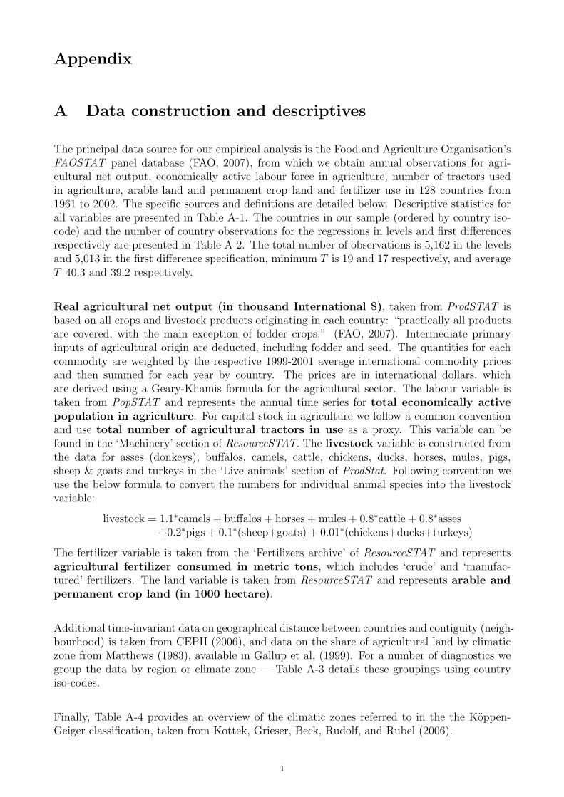
Appendix
A Data construction and descriptives
The principal data source for our empirical analysis is the Food and Agriculture Organisation’sFAOSTAT panel database (FAO, 2007), from which we obtain annual observations for agri-cultural net output, economically active labour force in agriculture, number of tractors usedin agriculture, arable land and permanent crop land and fertilizer use in 128 countries from1961 to 2002. The specific sources and definitions are detailed below. Descriptive statistics forall variables are presented in Table A-1. The countries in our sample (ordered by country iso-code) and the number of country observations for the regressions in levels and first differencesrespectively are presented in Table A-2. The total number of observations is 5,162 in the levelsand 5,013 in the first difference specification, minimum T is 19 and 17 respectively, and averageT 40.3 and 39.2 respectively.
Real agricultural net output (in thousand International $), taken from ProdSTAT isbased on all crops and livestock products originating in each country: “practically all productsare covered, with the main exception of fodder crops.” (FAO, 2007). Intermediate primaryinputs of agricultural origin are deducted, including fodder and seed. The quantities for eachcommodity are weighted by the respective 1999-2001 average international commodity pricesand then summed for each year by country. The prices are in international dollars, whichare derived using a Geary-Khamis formula for the agricultural sector. The labour variable istaken from PopSTAT and represents the annual time series for total economically activepopulation in agriculture. For capital stock in agriculture we follow a common conventionand use total number of agricultural tractors in use as a proxy. This variable can befound in the ‘Machinery’ section of ResourceSTAT. The livestock variable is constructed fromthe data for asses (donkeys), buffalos, camels, cattle, chickens, ducks, horses, mules, pigs,sheep & goats and turkeys in the ‘Live animals’ section of ProdStat. Following convention weuse the below formula to convert the numbers for individual animal species into the livestockvariable:
livestock = 1.1∗camels + buffalos + horses + mules + 0.8∗cattle + 0.8∗asses+0.2∗pigs + 0.1∗(sheep+goats) + 0.01∗(chickens+ducks+turkeys)
The fertilizer variable is taken from the ‘Fertilizers archive’ of ResourceSTAT and representsagricultural fertilizer consumed in metric tons, which includes ‘crude’ and ‘manufac-tured’ fertilizers. The land variable is taken from ResourceSTAT and represents arable andpermanent crop land (in 1000 hectare).
Additional time-invariant data on geographical distance between countries and contiguity (neigh-bourhood) is taken from CEPII (2006), and data on the share of agricultural land by climaticzone from Matthews (1983), available in Gallup et al. (1999). For a number of diagnostics wegroup the data by region or climate zone — Table A-3 details these groupings using countryiso-codes.
Finally, Table A-4 provides an overview of the climatic zones referred to in the the Koppen-Geiger classification, taken from Kottek, Grieser, Beck, Rudolf, and Rubel (2006).
i
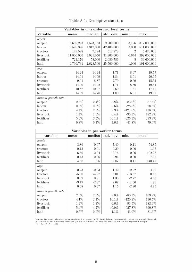
Table A-1: Descriptive statistics
Variables in untransformed level terms
Variable mean median std. dev. min. max.
levelsoutput 6,659,293 1,523,753 19,900,000 3,196 317,000,000labour 8,528,396 1,317,000 42,400,000 3,000 511,000,000tractors 149,528 7,124 512,278 2 5,470,000livestock 11,800,000 3,031,056 31,900,000 6,644 298,000,000fertilizer 721,176 58,000 2,680,786 5 39,600,000land 9,799,731 2,628,500 25,500,000 1,000 191,000,000
logsoutput 14.24 14.24 1.71 8.07 19.57labour 14.01 14.09 1.84 8.01 20.05tractors 9.01 8.87 2.79 0.69 15.51livestock 14.90 14.92 1.71 8.80 19.51fertilizer 10.82 10.97 2.69 1.61 17.49land 14.69 14.78 1.80 6.91 19.07
annual growth rateoutput 2.3% 2.4% 8.8% -83.0% 87.6%labour 0.3% 0.8% 2.6% -28.8% 28.8%tractors 4.4% 2.0% 9.9% -121.8% 138.6%livestock 1.4% 1.6% 6.4% -93.3% 182.9%fertilizer 5.6% 3.5% 40.1% -626.3% 393.2%land 0.8% 0.1% 3.6% -41.8% 79.0%
Variables in per worker terms
variable mean median std. dev. min. max.
levelsoutput 3.86 0.97 7.40 0.11 54.85tractors 0.13 0.01 0.29 0.00 1.97livestock 6.60 2.24 12.76 0.06 102.28fertilizer 0.43 0.06 0.94 0.00 7.05land 4.88 1.96 12.87 0.11 140.47
logsoutput 0.23 -0.03 1.42 -2.22 4.00tractors -5.00 -4.97 3.01 -13.67 0.68livestock 0.89 0.81 1.38 -2.77 4.63fertilizer -3.19 -2.87 2.67 -11.56 1.95land 0.68 0.67 1.15 -2.20 4.95
annual growth rateoutput 2.0% 2.0% 9.0% -80.3% 109.9%tractors 4.1% 2.1% 10.1% -120.2% 136.5%livestock 1.2% 1.2% 6.6% -93.5% 182.9%fertilizer 5.4% 4.2% 40.0% -627.8% 390.8%land 0.5% 0.0% 4.1% -43.0% 81.6%
Notes: We report the descriptive statistics for output (in I$1,000), labour (headcount), tractors (number), livestock(cattle-equivalent numbers), fertilizer (in metric tonnes) and land (in hectare) for the full regression sample(n = 5, 162; N = 128).
ii

Table A-2: Sample of countries and number of observations
Country Code levels FD Country Code levels FDAfghanistan AFG 40 38 Cambodia KHM 33 30Angola AGO 40 39 South Korea KOR 42 41Albania ALB 42 41 Kuwait KWT 24 22United Arab Emirates ARE 31 30 Lao PDR LAO 38 35Argentina ARG 42 41 Lebanon LBN 42 41Australia AUS 42 41 Liberia LBR 30 29Austria AUT 42 41 Libya LBY 42 41Burundi BDI 37 36 Sri Lanka LKA 42 41Benin BEN 42 41 Lesotho LSO 42 41Burkina Faso BFA 42 41 Morocco MAR 42 41Bangladesh BGD 42 41 Madagascar MDG 42 41Bulgaria BGR 42 41 Mexico MEX 42 41Belgium-Luxembourg BLX 39 38 Mali MLI 42 41Belize BLZ 42 41 Myanmar MMR 42 41Bolivia BOL 42 41 Mongolia MNG 34 33Brazil BRA 42 41 Mozambique MOZ 42 41Botswana BWA 42 41 Mauritania MRT 33 29Central African Republic CAF 42 41 Malawi MWI 42 41Canada CAN 42 41 Malaysia MYS 42 41Switzerland CHE 42 41 Niger NER 34 33Chile CHL 42 41 Nigeria NGA 42 41China CHN 42 41 Nicaragua NIC 42 41Cote d’Ivoire CIV 42 41 Netherlands NLD 42 41Cameroon CMR 42 41 Norway NOR 42 41Congo, Republic COG 41 39 Nepal NPL 42 41Colombia COL 42 41 New Zealand NZL 42 41Costa Rica CRI 42 41 Oman OMN 30 29Cuba CUB 42 41 Pakistan PAK 42 41Cyprus CYP 42 41 Panama PAN 42 41Germany DEU 42 41 Philippines PHL 42 41Denmark DNK 42 41 Papua New Guinea PNG 42 41Dominican Republic DOM 42 41 Poland POL 42 41Algeria DZA 42 41 Korea, DPR PRK 42 41Ecuador ECU 42 41 Portugal PRT 42 41Egypt EGY 42 41 Paraguay PRY 42 41Spain ESP 42 41 Qatar QAT 27 26Ethiopia ETH 42 41 Romania ROM 42 41Finland FIN 30 29 Rwanda RWA 34 32France FRA 42 41 Saudi Arabia SAU 42 41Gabon GAB 31 30 Sudan SDN 42 41United Kingdom GBR 42 41 Senegal SEN 42 41Ghana GHA 42 41 Sierra Leone SLE 42 41Guinea GIN 41 39 El Salvador SLV 42 41Gambia GMB 39 38 Somalia SOM 36 33Guinea-Bissau GNB 26 23 Suriname SUR 42 41Equatorial Guinea GNQ 19 17 Sweden SWE 42 41Greece GRC 42 41 Swaziland SWZ 42 41Guatemala GTM 42 41 Syria SYR 42 41Guyana GUY 42 41 Chad TCD 41 39Honduras HND 42 41 Togo TGO 37 36Haiti HTI 42 41 Thailand THA 42 41Hungary HUN 42 41 Trinidad & Tobago TTO 42 41Indonesia IDN 42 41 Tunisia TUN 42 41India IND 42 41 Turkey TUR 42 41Ireland IRL 42 41 Tanzania TZA 42 41Iran IRN 42 41 Uganda UGA 39 36Iraq IRQ 42 41 Uruguay URY 42 41Iceland ISL 42 41 United States USA 42 41Israel ISR 42 41 Venezuela VEN 42 41Italy ITA 42 41 Vietnam VNM 42 41Jamaica JAM 42 41 Yemen, Republic YEM 37 36Jordan JOR 42 41 South Africa ZAF 42 41Japan JPN 42 41 Congo, DR ZAR 41 39Kenya KEN 42 41 Zimbabwe ZWE 42 41
Notes: The full levels sample contains n=5,162 observations, the sample with variables in first differences (FD)contains n=5,013 observations. The sample period is from 1961 to 2002.
iii
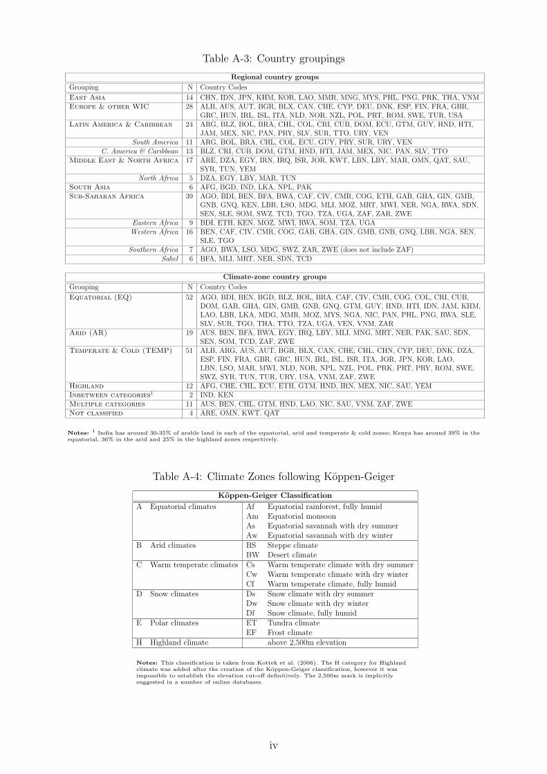
Table A-3: Country groupings
Regional country groups
Grouping N Country Codes
East Asia 14 CHN, IDN, JPN, KHM, KOR, LAO, MMR, MNG, MYS, PHL, PNG, PRK, THA, VNMEurope & other WIC 28 ALB, AUS, AUT, BGR, BLX, CAN, CHE, CYP, DEU, DNK, ESP, FIN, FRA, GBR,
GRC, HUN, IRL, ISL, ITA, NLD, NOR, NZL, POL, PRT, ROM, SWE, TUR, USALatin America & Caribbean 24 ARG, BLZ, BOL, BRA, CHL, COL, CRI, CUB, DOM, ECU, GTM, GUY, HND, HTI,
JAM, MEX, NIC, PAN, PRY, SLV, SUR, TTO, URY, VENSouth America 11 ARG, BOL, BRA, CHL, COL, ECU, GUY, PRY, SUR, URY, VEN
C. America & Caribbean 13 BLZ, CRI, CUB, DOM, GTM, HND, HTI, JAM, MEX, NIC, PAN, SLV, TTOMiddle East & North Africa 17 ARE, DZA, EGY, IRN, IRQ, ISR, JOR, KWT, LBN, LBY, MAR, OMN, QAT, SAU,
SYR, TUN, YEMNorth Africa 5 DZA, EGY, LBY, MAR, TUN
South Asia 6 AFG, BGD, IND, LKA, NPL, PAKSub-Saharan Africa 39 AGO, BDI, BEN, BFA, BWA, CAF, CIV, CMR, COG, ETH, GAB, GHA, GIN, GMB,
GNB, GNQ, KEN, LBR, LSO, MDG, MLI, MOZ, MRT, MWI, NER, NGA, RWA, SDN,SEN, SLE, SOM, SWZ, TCD, TGO, TZA, UGA, ZAF, ZAR, ZWE
Eastern Africa 9 BDI, ETH, KEN, MOZ, MWI, RWA, SOM, TZA, UGAWestern Africa 16 BEN, CAF, CIV, CMR, COG, GAB, GHA, GIN, GMB, GNB, GNQ, LBR, NGA, SEN,
SLE, TGOSouthern Africa 7 AGO, BWA, LSO, MDG, SWZ, ZAR, ZWE (does not include ZAF)
Sahel 6 BFA, MLI, MRT, NER, SDN, TCD
Climate-zone country groups
Grouping N Country Codes
Equatorial (EQ) 52 AGO, BDI, BEN, BGD, BLZ, BOL, BRA, CAF, CIV, CMR, COG, COL, CRI, CUB,DOM, GAB, GHA, GIN, GMB, GNB, GNQ, GTM, GUY, HND, HTI, IDN, JAM, KHM,LAO, LBR, LKA, MDG, MMR, MOZ, MYS, NGA, NIC, PAN, PHL, PNG, RWA, SLE,SLV, SUR, TGO, THA, TTO, TZA, UGA, VEN, VNM, ZAR
Arid (AR) 19 AUS, BEN, BFA, BWA, EGY, IRQ, LBY, MLI, MNG, MRT, NER, PAK, SAU, SDN,SEN, SOM, TCD, ZAF, ZWE
Temperate & Cold (TEMP) 51 ALB, ARG, AUS, AUT, BGR, BLX, CAN, CHE, CHL, CHN, CYP, DEU, DNK, DZA,ESP, FIN, FRA, GBR, GRC, HUN, IRL, ISL, ISR, ITA, JOR, JPN, KOR, LAO,LBN, LSO, MAR, MWI, NLD, NOR, NPL, NZL, POL, PRK, PRT, PRY, ROM, SWE,SWZ, SYR, TUN, TUR, URY, USA, VNM, ZAF, ZWE
Highland 12 AFG, CHE, CHL, ECU, ETH, GTM, HND, IRN, MEX, NIC, SAU, YEMInbetween categories1 2 IND, KENMultiple categories 11 AUS, BEN, CHL, GTM, HND, LAO, NIC, SAU, VNM, ZAF, ZWENot classified 4 ARE, OMN, KWT, QAT
Notes: 1 India has around 30-35% of arable land in each of the equatorial, arid and temperate & cold zones; Kenya has around 39% in theequatorial, 36% in the arid and 25% in the highland zones respectively.
Table A-4: Climate Zones following Koppen-Geiger
Koppen-Geiger Classification
A Equatorial climates Af Equatorial rainforest, fully humidAm Equatorial monsoonAs Equatorial savannah with dry summerAw Equatorial savannah with dry winter
B Arid climates BS Steppe climateBW Desert climate
C Warm temperate climates Cs Warm temperate climate with dry summerCw Warm temperate climate with dry winterCf Warm temperate climate, fully humid
D Snow climates Ds Snow climate with dry summerDw Snow climate with dry winterDf Snow climate, fully humid
E Polar climates ET Tundra climateEF Frost climate
H Highland climate above 2,500m elevation
Notes: This classification is taken from Kottek et al. (2006). The H category for Highlandclimate was added after the creation of the Koppen-Geiger classification, however it wasimpossible to establish the elevation cut-off definitively. The 2,500m mark is implicitlysuggested in a number of online databases.
iv

B Time-series properties of the data
In this section we report results relating to the time-series properties of the data. Since the timedimension of the panel is sizeable (T ranges from 19 to 42, average T = 40.3), we first carry outAugmented Dickey-Fuller (Dickey & Fuller, 1979) and KPSS (Kwiatkowski, Phillips, Schmidt,& Shin, 1992) tests for the variable series within each individual country.14 We use this com-bination of tests since the ADF test has the null of nonstationary variable series, whereas theKPSS test has the null of stationary variable series. The time-series unit root test rejectionfrequencies for variables in levels and in first differences are shown in Table B-1: we reportthe share of countries (in %) for which the null hypothesis (stationarity or nonstationarity asindicated) is rejected. The theoretical rejection frequencies at our sample size are 12.8% (H0 :nonstationarity) and 87.2% (H0 : stationarity) for the 10% significance level we adopted.
Table B-1: Time-series unit root tests — rejection frequency
Unit root testsshare of country tests which reject H0 (stationarity or nonstationarity as indicated);
no adjustment for cross-sectional dependence; all variables in logs
Testing for levels-stationarity
Test log output pw labour tractors pw livestock pw fertilizer pw land pwADF without trend H0: nonstationary H1: levels-stationary 9% 9% 48% 16% 41% 10%KPSS without trend H0: levels-stationary H1: nonstationary 82% 91% 81% 85% 70% 82%
Testing for trend-stationarity
Test output pw labour tractors pw livestock pw fertilizer pw land pwADF with trend H0: nonstationary H1: trend-stationary 16% 15% 24% 12% 21% 11%KPSS with trend H0: trend-stationary H1: nonstationary 65% 71% 88% 65% 74% 66%
Testing for difference-stationarity
Test output pw labour tractors pw livestock pw fertilizer pw land pwADF with drift H0: nonstationary H1: stationary 94% 16% 48% 88% 78% 67%KPSS with drift H0: stationary H1: nonstationary 13% 38% 81% 81% 70% 82%
Notes: All variables are in logs. We report the share of countries (out of N = 128) for which the respective unit root test is rejected at the 10%level of significance. All unit root tests for variables in levels contain an intercept term in the estimating equation. ADF refers to the augmentedDickey-Fuller test, which has the null of nonstationarity. KPSS refers to the Kwiatkowski et al. (1992) unit root test, which has the null of(trend-)stationarity. Lag-augmentation or bandwidth selection in these tests to account for serial correlation in the variables is allowed to vary bycountry. For the ADF test we determined ‘ideal’ lag-augmentation using the Akaike Information Criterion (AIC). For the KPSS tests anautomated bandwidth selection following Newey and West (1994) and discussed in Hobijn et al. (2004) is used. For KPSS we use the kpss
command in Stata written by Kit Baum.
For the majority of countries the ADF tests for the variables in levels cannot reject nonstation-arity, with the notable exceptions of tractors per worker and fertilizer per worker. Consistentlywith this finding the majority of country KPSS tests reject the null of level stationarity. Thetests for trend stationarity reveal a similar pattern. The difference stationarity tests showconsiderable differences across variables: in the ADF tests the labour and tractors per workervariables reject the nonstationarity null in far less countries than we would expect (87.2%) andthe KPSS tests reject stationarity in the vast majority of countries for the tractors, livestock,fertilizer and land (all in per worker terms) variables.
Our analysis based on standard time-series (non)stationarity tests therefore has no clearcutmessage regarding variable properties. It needs to be emphasised that country-specific unitroot tests suffer from low power, in particular in the case where the persistence in the variableis high — i.e. in the case when the test matters most (Harris, 1994).
14Whereas the Stata command for ADF allows us to run country regressions with gaps in the data, this isnot possible for the KPSS tests. We interpolate data in order to run the KPSS for a balanced panel.
v

Next we apply ‘first generation’ panel unit root tests to the data. These were devel-oped due to the desirable property of increased power from pooling the results from manylow-powered country unit root tests. It is important to stress that rejection of the unit rootnull hypothesis does not imply that the panel is stationary, but rather that the variable seriesdoes not follow a unit root process in all countries. Table B-2 presents the results for theMaddala and Wu (1999) (MW) panel unit root test and a panel version of Phillips and Perron(1988) (PP) test, for which serial correlation is accounted for using nonparametric methodsrather than lagged differences. Following Fisher’s suggestion the MW statistic is constructedas P = −2
∑i log(pi), where pi is the p-value for the individual country ADF statistics. The
PP test is constructed in analogy. For both tests the theoretical distribution of the statistic isχ2(2N), s.t. critical values are 97.35 for 5% and 92.16 for 10%.
For both tests tractors per worker and fertilizer per worker in levels reject nonstationarity inboth the standard ADF equation and the ADF equation with a trend. All other variables inlevels seemingly cannot reject the null of nonstationarity once augmented with sufficient lagsor once a trend is added to the ADF equation. For the variables in first differences the testsunanimously reject nonstationarity.
Similarly to the above analysis we cannot definitely reject nonstationarity in all variables. How-ever, as Baltagi et al. (2007) point out the first generation panel unit root tests which do notaccount for cross-section dependence can be subject to considerable size distortions, such thatthe test tends to overreject. This issue led to the development of ‘second generation’ panelunit root tests, namely the Im, Pesaran, and Shin (2003) and the Pesaran (2007) tests, resultsfor which are presented in Table B-3. These tests explicitly allow for cross-sectional dependencein the data and therefore have better performance than the ‘classic’ panel unit root tests thatassume cross-sectional independence.
Our results now seem to provide a more consistent theme across the different variables andspecifications: following augmentation with lags or a linear trend term the levels variables can-not reject the null of nonstationarity. For the variables in first differences all variables rejectnonstationarity with the exception of labour.
It should be noted that our preferred panel unit root test by Pesaran (2007) can only accountfor a single unobserved common factor as the cause for cross-sectional dependence in the data.More recent extensions of this test (Pesaran et al., 2008) can accommodate multiple unob-served common factors, but this development was too recent for the test to be included inthis paper. Further issues which have received attention in the recent panel unit root litera-ture such as structural breaks in data series (Westerlund, 2006; Kao, Trapani, & Urga, 2007)and changes in the volatility of the innovations (Hanck, 2008) could also not be accommodated.
vi
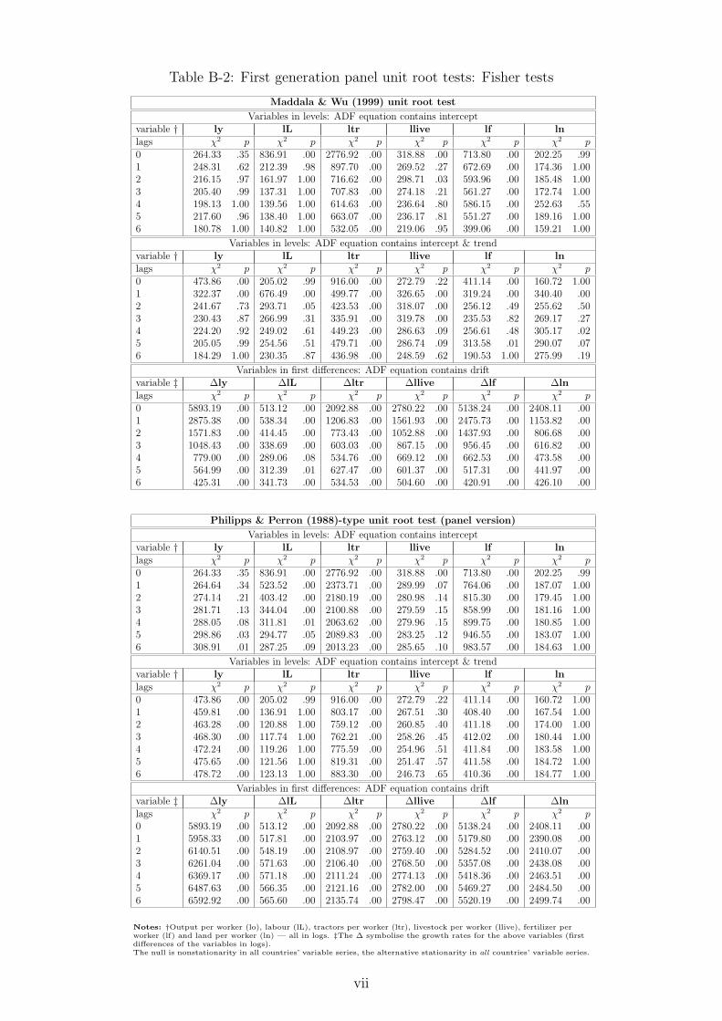
Table B-2: First generation panel unit root tests: Fisher tests
Maddala & Wu (1999) unit root test
Variables in levels: ADF equation contains interceptvariable † ly lL ltr llive lf lnlags χ2 p χ2 p χ2 p χ2 p χ2 p χ2 p0 264.33 .35 836.91 .00 2776.92 .00 318.88 .00 713.80 .00 202.25 .991 248.31 .62 212.39 .98 897.70 .00 269.52 .27 672.69 .00 174.36 1.002 216.15 .97 161.97 1.00 716.62 .00 298.71 .03 593.96 .00 185.48 1.003 205.40 .99 137.31 1.00 707.83 .00 274.18 .21 561.27 .00 172.74 1.004 198.13 1.00 139.56 1.00 614.63 .00 236.64 .80 586.15 .00 252.63 .555 217.60 .96 138.40 1.00 663.07 .00 236.17 .81 551.27 .00 189.16 1.006 180.78 1.00 140.82 1.00 532.05 .00 219.06 .95 399.06 .00 159.21 1.00
Variables in levels: ADF equation contains intercept & trendvariable † ly lL ltr llive lf lnlags χ2 p χ2 p χ2 p χ2 p χ2 p χ2 p0 473.86 .00 205.02 .99 916.00 .00 272.79 .22 411.14 .00 160.72 1.001 322.37 .00 676.49 .00 499.77 .00 326.65 .00 319.24 .00 340.40 .002 241.67 .73 293.71 .05 423.53 .00 318.07 .00 256.12 .49 255.62 .503 230.43 .87 266.99 .31 335.91 .00 319.78 .00 235.53 .82 269.17 .274 224.20 .92 249.02 .61 449.23 .00 286.63 .09 256.61 .48 305.17 .025 205.05 .99 254.56 .51 479.71 .00 286.74 .09 313.58 .01 290.07 .076 184.29 1.00 230.35 .87 436.98 .00 248.59 .62 190.53 1.00 275.99 .19
Variables in first differences: ADF equation contains driftvariable ‡ ∆ly ∆lL ∆ltr ∆llive ∆lf ∆lnlags χ2 p χ2 p χ2 p χ2 p χ2 p χ2 p0 5893.19 .00 513.12 .00 2092.88 .00 2780.22 .00 5138.24 .00 2408.11 .001 2875.38 .00 538.34 .00 1206.83 .00 1561.93 .00 2475.73 .00 1153.82 .002 1571.83 .00 414.45 .00 773.43 .00 1052.88 .00 1437.93 .00 806.68 .003 1048.43 .00 338.69 .00 603.03 .00 867.15 .00 956.45 .00 616.82 .004 779.00 .00 289.06 .08 534.76 .00 669.12 .00 662.53 .00 473.58 .005 564.99 .00 312.39 .01 627.47 .00 601.37 .00 517.31 .00 441.97 .006 425.31 .00 341.73 .00 534.53 .00 504.60 .00 420.91 .00 426.10 .00
Philipps & Perron (1988)-type unit root test (panel version)
Variables in levels: ADF equation contains interceptvariable † ly lL ltr llive lf lnlags χ2 p χ2 p χ2 p χ2 p χ2 p χ2 p0 264.33 .35 836.91 .00 2776.92 .00 318.88 .00 713.80 .00 202.25 .991 264.64 .34 523.52 .00 2373.71 .00 289.99 .07 764.06 .00 187.07 1.002 274.14 .21 403.42 .00 2180.19 .00 280.98 .14 815.30 .00 179.45 1.003 281.71 .13 344.04 .00 2100.88 .00 279.59 .15 858.99 .00 181.16 1.004 288.05 .08 311.81 .01 2063.62 .00 279.96 .15 899.75 .00 180.85 1.005 298.86 .03 294.77 .05 2089.83 .00 283.25 .12 946.55 .00 183.07 1.006 308.91 .01 287.25 .09 2013.23 .00 285.65 .10 983.57 .00 184.63 1.00
Variables in levels: ADF equation contains intercept & trendvariable † ly lL ltr llive lf lnlags χ2 p χ2 p χ2 p χ2 p χ2 p χ2 p0 473.86 .00 205.02 .99 916.00 .00 272.79 .22 411.14 .00 160.72 1.001 459.81 .00 136.91 1.00 803.17 .00 267.51 .30 408.40 .00 167.54 1.002 463.28 .00 120.88 1.00 759.12 .00 260.85 .40 411.18 .00 174.00 1.003 468.30 .00 117.74 1.00 762.21 .00 258.26 .45 412.02 .00 180.44 1.004 472.24 .00 119.26 1.00 775.59 .00 254.96 .51 411.84 .00 183.58 1.005 475.65 .00 121.56 1.00 819.31 .00 251.47 .57 411.58 .00 184.72 1.006 478.72 .00 123.13 1.00 883.30 .00 246.73 .65 410.36 .00 184.77 1.00
Variables in first differences: ADF equation contains driftvariable ‡ ∆ly ∆lL ∆ltr ∆llive ∆lf ∆lnlags χ2 p χ2 p χ2 p χ2 p χ2 p χ2 p0 5893.19 .00 513.12 .00 2092.88 .00 2780.22 .00 5138.24 .00 2408.11 .001 5958.33 .00 517.81 .00 2103.97 .00 2763.12 .00 5179.80 .00 2390.08 .002 6140.51 .00 548.19 .00 2108.97 .00 2759.40 .00 5284.52 .00 2410.07 .003 6261.04 .00 571.63 .00 2106.40 .00 2768.50 .00 5357.08 .00 2438.08 .004 6369.17 .00 571.18 .00 2111.24 .00 2774.13 .00 5418.36 .00 2463.51 .005 6487.63 .00 566.35 .00 2121.16 .00 2782.00 .00 5469.27 .00 2484.50 .006 6592.92 .00 565.60 .00 2135.74 .00 2798.47 .00 5520.19 .00 2499.74 .00
Notes: †Output per worker (lo), labour (lL), tractors per worker (ltr), livestock per worker (llive), fertilizer perworker (lf) and land per worker (ln) — all in logs. ‡The ∆ symbolise the growth rates for the above variables (firstdifferences of the variables in logs).The null is nonstationarity in all countries’ variable series, the alternative stationarity in all countries’ variable series.
vii
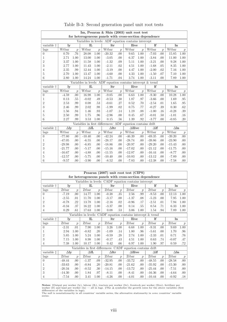
Table B-3: Second generation panel unit root tests
Im, Pesaran & Shin (2003) unit root testfor heterogeneous panels with cross-section dependence
Variables in levels: ADF equation contains interceptvariable † ly lL ltr llive lf lnlags Wtbar p Wtbar p Wtbar p Wtbar p Wtbar p Wtbar p0 0.70 .76 28.08 1.00 -20.32 .00 9.65 1.00 -7.03 .00 15.85 1.001 2.71 1.00 13.00 1.00 -3.05 .00 6.37 1.00 -3.84 .00 11.00 1.002 3.37 1.00 11.58 1.00 -1.32 .09 5.11 1.00 -3.21 .00 9.28 1.003 2.77 1.00 11.43 1.00 -2.11 .02 4.51 1.00 -1.68 .05 8.35 1.004 2.35 .99 12.44 1.00 -3.19 .00 4.47 1.00 -2.00 .02 7.16 1.005 2.70 1.00 13.47 1.00 -4.60 .00 4.33 1.00 -1.50 .07 7.10 1.006 2.80 1.00 14.24 1.00 -1.71 .04 3.74 1.00 -3.11 .00 7.89 1.00
Variables in levels: ADF equation contains intercept & trendvariable † ly lL ltr llive lf lnlags Wtbar p Wtbar p Wtbar p Wtbar p Wtbar p Wtbar p0 -4.59 .00 16.98 1.00 -9.05 .00 6.63 1.00 -9.30 .00 10.28 1.001 0.13 .55 -0.02 .49 -0.53 .30 1.87 .97 -3.66 .00 1.69 .952 2.53 .99 0.08 .53 -0.61 .27 0.52 .70 -2.54 .01 1.65 .953 2.46 .99 2.02 .98 -1.99 .02 0.75 .77 -0.27 .39 0.30 .624 1.56 .94 1.46 .93 -1.07 .14 1.19 .88 -1.00 .16 -0.28 .395 2.50 .99 1.75 .96 -2.96 .00 0.45 .67 -0.01 .50 -1.01 .166 2.27 .99 3.53 1.00 0.15 .56 1.39 .92 -3.77 .00 -0.85 .20
Variables in first differences: ADF equation contains driftvariable ‡ ∆ly ∆lL ∆ltr ∆llive ∆lf ∆lnlags Wtbar p Wtbar p Wtbar p Wtbar p Wtbar p Wtbar p0 -77.80 .00 -10.40 .00 -42.24 .00 -46.39 .00 -69.35 .00 -39.20 .001 -47.05 .00 -6.55 .00 -28.17 .00 -28.74 .00 -39.86 .00 -23.90 .002 -29.98 .00 -6.85 .00 -18.86 .00 -20.97 .00 -29.20 .00 -15.43 .003 -21.77 .00 -5.17 .00 -15.16 .00 -17.02 .00 -21.12 .00 -11.75 .004 -16.67 .00 -4.88 .00 -11.55 .00 -12.87 .00 -16.44 .00 -8.77 .005 -12.57 .00 -5.75 .00 -10.40 .00 -10.83 .00 -13.12 .00 -7.89 .006 -9.57 .00 -3.90 .00 -8.52 .00 -7.83 .00 -12.38 .00 -7.58 .00
Pesaran (2007) unit root test (CIPS)for heterogeneous panels with cross-section dependence
Variables in levels: CADF equation contains interceptvariable † ly lL ltr llive lf lnlags Ztbar p Ztbar p Ztbar p Ztbar p Ztbar p Ztbar p0 -7.19 .00 14.77 1.00 -0.38 .35 2.56 .99 -9.53 .00 12.13 1.001 -2.55 .01 11.70 1.00 -3.17 .00 -1.37 .08 -5.23 .00 7.95 1.002 -0.78 .22 13.78 1.00 -2.16 .02 -0.96 .17 -2.51 .01 7.94 1.003 -0.34 .37 16.22 1.00 -3.37 .00 0.14 .55 0.54 .71 6.33 1.004 0.29 .61 17.63 1.00 0.08 .53 3.06 1.00 1.54 .94 7.89 1.00
Variables in levels: CADF equation contains intercept & trendvariable † ly lL ltr llive lf lnlags Ztbar p Ztbar p Ztbar p Ztbar p Ztbar p Ztbar p0 -2.31 .01 7.90 1.00 3.26 1.00 6.68 1.00 -9.31 .00 9.69 1.001 2.94 1.00 -0.82 .20 -1.09 .14 1.80 .96 -5.61 .00 1.70 .962 5.85 1.00 5.24 1.00 -0.59 .28 2.74 1.00 -2.33 .01 0.71 .763 7.15 1.00 8.98 1.00 -0.17 .43 4.51 1.00 0.63 .74 -0.07 .474 7.38 1.00 10.17 1.00 0.42 .66 6.97 1.00 1.90 .97 0.59 .72
Variables in first differences: CADF equation contains driftvariable ‡ ∆ly ∆lL ∆ltr ∆llive ∆lf ∆lnlags Ztbar p Ztbar p Ztbar p Ztbar p Ztbar p Ztbar p0 -48.44 .00 -1.37 .09 -32.95 .00 -33.72 .00 -48.55 .00 -28.58 .001 -33.63 .00 -0.84 .20 -20.81 .00 -21.62 .00 -35.92 .00 -15.30 .002 -20.34 .00 -0.52 .30 -14.15 .00 -13.72 .00 -25.44 .00 -7.51 .003 -14.30 .00 1.84 .97 -8.11 .00 -8.41 .00 -16.36 .00 -4.64 .004 -7.54 .00 3.41 1.00 -4.26 .00 -4.01 .00 -10.44 .00 -0.92 .18
Notes: †Output per worker (ly), labour (lL), tractors per worker (ltr), livestock per worker (llive), fertilizer perworker (lf) and land per worker (ln) — all in logs. ‡The ∆ symbolise the growth rates for the above variables (firstdifferences of the variables in logs).The null is nonstationarity in all countries’ variable series, the alternative stationarity in some countries’ variableseries.
viii
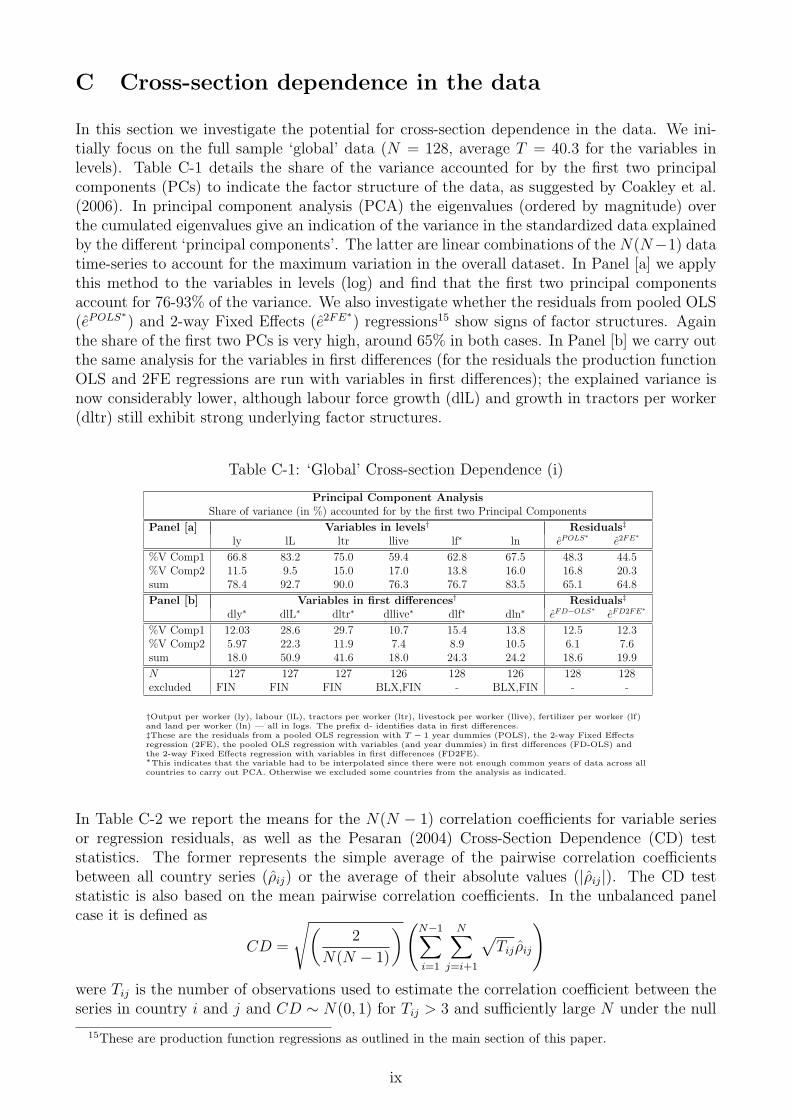
C Cross-section dependence in the data
In this section we investigate the potential for cross-section dependence in the data. We ini-tially focus on the full sample ‘global’ data (N = 128, average T = 40.3 for the variables inlevels). Table C-1 details the share of the variance accounted for by the first two principalcomponents (PCs) to indicate the factor structure of the data, as suggested by Coakley et al.(2006). In principal component analysis (PCA) the eigenvalues (ordered by magnitude) overthe cumulated eigenvalues give an indication of the variance in the standardized data explainedby the different ‘principal components’. The latter are linear combinations of the N(N−1) datatime-series to account for the maximum variation in the overall dataset. In Panel [a] we applythis method to the variables in levels (log) and find that the first two principal componentsaccount for 76-93% of the variance. We also investigate whether the residuals from pooled OLS(ePOLS
∗) and 2-way Fixed Effects (e2FE
∗) regressions15 show signs of factor structures. Again
the share of the first two PCs is very high, around 65% in both cases. In Panel [b] we carry outthe same analysis for the variables in first differences (for the residuals the production functionOLS and 2FE regressions are run with variables in first differences); the explained variance isnow considerably lower, although labour force growth (dlL) and growth in tractors per worker(dltr) still exhibit strong underlying factor structures.
Table C-1: ‘Global’ Cross-section Dependence (i)
Principal Component AnalysisShare of variance (in %) accounted for by the first two Principal Components
Panel [a] Variables in levels† Residuals‡
ly lL ltr llive lf∗ ln ePOLS∗
e2FE∗
%V Comp1 66.8 83.2 75.0 59.4 62.8 67.5 48.3 44.5%V Comp2 11.5 9.5 15.0 17.0 13.8 16.0 16.8 20.3sum 78.4 92.7 90.0 76.3 76.7 83.5 65.1 64.8
Panel [b] Variables in first differences† Residuals‡
dly∗ dlL∗ dltr∗ dllive∗ dlf∗ dln∗ eFD−OLS∗
eFD2FE∗
%V Comp1 12.03 28.6 29.7 10.7 15.4 13.8 12.5 12.3%V Comp2 5.97 22.3 11.9 7.4 8.9 10.5 6.1 7.6sum 18.0 50.9 41.6 18.0 24.3 24.2 18.6 19.9
N 127 127 127 126 128 126 128 128excluded FIN FIN FIN BLX,FIN - BLX,FIN - -
†Output per worker (ly), labour (lL), tractors per worker (ltr), livestock per worker (llive), fertilizer per worker (lf)and land per worker (ln) — all in logs. The prefix d- identifies data in first differences.‡These are the residuals from a pooled OLS regression with T − 1 year dummies (POLS), the 2-way Fixed Effectsregression (2FE), the pooled OLS regression with variables (and year dummies) in first differences (FD-OLS) andthe 2-way Fixed Effects regression with variables in first differences (FD2FE).∗This indicates that the variable had to be interpolated since there were not enough common years of data across allcountries to carry out PCA. Otherwise we excluded some countries from the analysis as indicated.
In Table C-2 we report the means for the N(N − 1) correlation coefficients for variable seriesor regression residuals, as well as the Pesaran (2004) Cross-Section Dependence (CD) teststatistics. The former represents the simple average of the pairwise correlation coefficientsbetween all country series (ρij) or the average of their absolute values (|ρij|). The CD teststatistic is also based on the mean pairwise correlation coefficients. In the unbalanced panelcase it is defined as
CD =
√(2
N(N − 1)
)(N−1∑i=1
N∑j=i+1
√Tij ρij
)were Tij is the number of observations used to estimate the correlation coefficient between theseries in country i and j and CD ∼ N(0, 1) for Tij > 3 and sufficiently large N under the null
15These are production function regressions as outlined in the main section of this paper.
ix
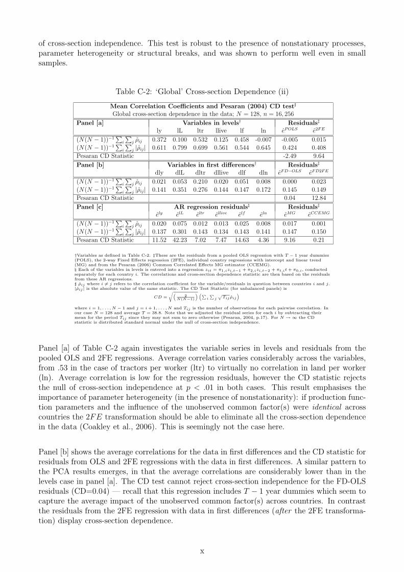
of cross-section independence. This test is robust to the presence of nonstationary processes,parameter heterogeneity or structural breaks, and was shown to perform well even in smallsamples.
Table C-2: ‘Global’ Cross-section Dependence (ii)
Mean Correlation Coefficients and Pesaran (2004) CD test]
Global cross-section dependence in the data; N = 128, n = 16, 256
Panel [a] Variables in levels† Residuals‡
ly lL ltr llive lf ln ePOLS e2FE
(N(N − 1))−1∑
i
∑j ρij 0.372 0.100 0.532 0.125 0.458 -0.007 -0.005 0.015
(N(N − 1))−1∑
i
∑j |ρij| 0.611 0.799 0.699 0.561 0.544 0.645 0.424 0.408
Pesaran CD Statistic -2.49 9.64
Panel [b] Variables in first differences† Residuals‡
dly dlL dltr dllive dlf dln eFD−OLS eFD2FE
(N(N − 1))−1∑
i
∑j ρij 0.021 0.053 0.210 0.020 0.051 0.008 0.000 0.023
(N(N − 1))−1∑
i
∑j |ρij| 0.141 0.351 0.276 0.144 0.147 0.172 0.145 0.149
Pesaran CD Statistic 0.04 12.84
Panel [c] AR regression residuals\ Residuals‡
ely elL eltr ellive elf eln eMG eCCEMG
(N(N − 1))−1∑
i
∑j ρij 0.020 0.075 0.012 0.013 0.025 0.008 0.017 0.001
(N(N − 1))−1∑
i
∑j |ρij| 0.137 0.301 0.143 0.134 0.143 0.141 0.147 0.150
Pesaran CD Statistic 11.52 42.23 7.02 7.47 14.63 4.36 9.16 0.21
†Variables as defined in Table C-2. ‡These are the residuals from a pooled OLS regression with T − 1 year dummies(POLS), the 2-way Fixed Effects regression (2FE), individual country regressions with intercept and linear trend(MG) and from the Pesaran (2006) Common Correlated Effects MG estimator (CCEMG).\ Each of the variables in levels is entered into a regression zit = π1,izi,t−1 + π2,izi,t−2 + πt,it + π0,i, conductedseparately for each country i. The correlations and cross-section dependence statistic are then based on the residualsfrom these AR regressions.] ρij where i 6= j refers to the correlation coefficient for the variable/residuals in question between countries i and j.|ρij | is the absolute value of the same statistic. The CD Test Statistic (for unbalanced panels) is
CD =
√(2
N(N−1)
) (∑i
∑j
√Tij ρij
)where i = 1, . . . , N − 1 and j = i + 1, . . . , N and Tij is the number of observations for each pairwise correlation. Inour case N = 128 and average T = 38.8. Note that we adjusted the residual series for each i by subtracting theirmean for the period Tij since they may not sum to zero otherwise (Pesaran, 2004, p.17). For N →∞ the CDstatistic is distributed standard normal under the null of cross-section independence.
Panel [a] of Table C-2 again investigates the variable series in levels and residuals from thepooled OLS and 2FE regressions. Average correlation varies considerably across the variables,from .53 in the case of tractors per worker (ltr) to virtually no correlation in land per worker(ln). Average correlation is low for the regression residuals, however the CD statistic rejectsthe null of cross-section independence at p < .01 in both cases. This result emphasises theimportance of parameter heterogeneity (in the presence of nonstationarity): if production func-tion parameters and the influence of the unobserved common factor(s) were identical acrosscountries the 2FE transformation should be able to eliminate all the cross-section dependencein the data (Coakley et al., 2006). This is seemingly not the case here.
Panel [b] shows the average correlations for the data in first differences and the CD statistic forresiduals from OLS and 2FE regressions with the data in first differences. A similar pattern tothe PCA results emerges, in that the average correlations are considerably lower than in thelevels case in panel [a]. The CD test cannot reject cross-section independence for the FD-OLSresiduals (CD=0.04) — recall that this regression includes T − 1 year dummies which seem tocapture the average impact of the unobserved common factor(s) across countries. In contrastthe residuals from the 2FE regression with data in first differences (after the 2FE transforma-tion) display cross-section dependence.
x
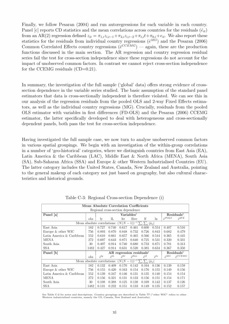
Finally, we follow Pesaran (2004) and run autoregressions for each variable in each country.Panel [c] reports CD statistics and the mean correlations across countries for the residuals (eit)from an AR(2) regression defined zit = π1,izi,t−1+π2,izi,t−2+πt,it+π0,i+eit. We also report thesestatistics for the residuals from individual country regressions (eMG) and the Pesaran (2006)Common Correlated Effects country regressions (eCCEMG) — again, these are the productionfunctions discussed in the main section. The AR regression and country regression residualseries fail the test for cross-section independence since these regressions do not account for theimpact of unobserved common factors. In contrast we cannot reject cross-section independencefor the CCEMG residuals (CD=0.21).
In summary, the investigation of the full sample (‘global’ data) offers strong evidence of cross-section dependence in the variable series studied. The basic assumption of the standard panelestimators that data is cross-sectionally independent is therefore violated. We can see this inour analysis of the regression residuals from the pooled OLS and 2-way Fixed Effects estima-tors, as well as the individual country regressions (MG). Crucially, residuals from the pooledOLS estimator with variables in first differences (FD-OLS) and the Pesaran (2006) CCEMGestimator, the latter specifically developed to deal with heterogeneous and cross-sectionallydependent panels, both pass the test for cross-section independence.
Having investigated the full sample case, we now turn to analyse unobserved common factorsin various spatial groupings. We begin with an investigation of the within-group correlationsin a number of ‘geo-historical’ categories, where we distinguish countries from East Asia (EA),Latin America & the Caribbean (LAC), Middle East & North Africa (MENA), South Asia(SA), Sub-Saharan Africa (SSA) and Europe & other Western Industrialised Countries (EU).The latter category includes the United States, Canada, New Zealand and Australia, pointingto the general makeup of each category not just based on geography, but also cultural charac-teristics and historical grounds.
Table C-3: Regional Cross-section Dependence (i)
Mean Absolute Correlation CoefficientsRegional cross-section dependence
Panel [a] Variables† Residuals‡
obs ly lL ltr llive lf ln ePOLS e2FE
Mean absolute correlations: (N(N − 1))−1∑
i
∑j |ρij|
East Asia 182 0.727 0.740 0.617 0.461 0.600 0.554 0.407 0.516Europe & other WIC 756 0.893 0.870 0.848 0.732 0.726 0.843 0.682 0.479Latin America & Caribbean 552 0.610 0.661 0.657 0.465 0.566 0.544 0.365 0.445MENA 272 0.697 0.643 0.871 0.640 0.725 0.531 0.320 0.331South Asia 30 0.497 0.914 0.740 0.680 0.733 0.871 0.781 0.313SSA 1482 0.427 0.914 0.631 0.520 0.385 0.634 0.367 0.350
Panel [b] AR regression residuals\ Residuals‡
obs ely elL eltr ellive elf eln eMG eCCEMG
Mean absolute correlations: (N(N − 1))−1∑
i
∑j |ρij|
East Asia 182 0.132 0.409 0.170 0.142 0.164 0.136 0.139 0.159Europe & other WIC 756 0.155 0.420 0.163 0.154 0.176 0.155 0.149 0.156Latin America & Caribbean 552 0.139 0.347 0.146 0.131 0.135 0.140 0.154 0.154MENA 272 0.156 0.321 0.131 0.133 0.156 0.151 0.154 0.171South Asia 30 0.108 0.388 0.125 0.138 0.169 0.142 0.137 0.126SSA 1482 0.131 0.232 0.151 0.133 0.149 0.135 0.152 0.157
See Table C-2 for notes and descriptions. Country groupings are described in Table ?? (”other WIC” refers to otherWestern industrialised countries, namely the US, Canada, New Zealand and Australia).
xi

Table C-3 presents variable (and residual) mean absolute correlations (we omit the mean stan-dard correlations to save space) within each of these country groupings. The number of obser-vations ranges from 30 in South Asia (N = 6) to 1,482 in Sub-Saharan Africa (N = 39). Inpanel [a] we report results for the variables in levels and the regression residuals from OLS and2FE regressions. All variables are uniformly highly correlated within country groupings. Forthe regression residuals in particular the members of the Europe & WIC and East Asia groupsshow high levels of correlation.16 In panel [b] we investigate residuals from the autoregressionsoutlined above as well as the country regressions and CCE country regressions. All of theseshow significantly lower levels of correlation. Average correlation (not reported) shows a muchhigher range of correlation coefficients across the groups, in the case of land from -.06 in EastAsia to .58 in Europe & WIC and .87 in South Asia. In the latter analysis regression residualsfrom POLS and 2FE remain high in the Europe & WIC case (.41 and .28 respectively), butare virtually insignificant in the MG and CCEMG case (.05 and .02).
In Table C-4 we present the results for the CD test statistic within and across regions appliedto various regression residuals. Panels [a] to [e] are for the pooled OLS (POLS), 2-way FixedEffects (2FE), OLS in first differences (FD-OLS), country regression and CCE country regres-sion residuals respectively. Panel [f] shows the number of observations (pairwise correlations)for each test. We marked the test statistics which indicate rejection of the null of cross-sectionindependence in bold.
Focusing first on the within-group CD test statistics (on the diagonals), we can see that thesecommonly reject cross-section independence across all estimation strategies, although less soin the country and CCEMG regression cases. With regard to cross-group dependence tests,it can be seen that residuals from the pooled regression in levels and the pooled 2FE regres-sion display a high level of common factor structure, leading to the rejection of the null ofcross-section independence in almost all cases. For the pooled regression with variables in firstdifferences 10 out of 15 cross-group tests cannot reject the null of cross-section independence,whereas for country regressions 12 tests cannot reject. For CCEMG all 15 tests cannot rejectindependence across groups. The results in panel [e] for CCEMG residuals suggests that thisestimation approach cannot entirely wipe out the cross-section dependence in the data if viewedfrom a group-perspective. It is no longer the case that the number of observations is systemat-ically linked to the test statistic, suggesting that the results are not driven by small sample size.
In Table C-5 we apply an alternative ‘spatial’ grouping, whereby the share of arable land in oneof three eco-climatic zones determines group membership. We use data from Matthews (1983),reported in Gallup et al. (1999), on this variable and group countries into equatorial (EQ), arid(AR) or temperate & cold (TEMP) climate zones if they have 40% or more arable land sharein the respective climatic zone. We provide details on the countries that drop out of the sampleas a result of this categorisation and the treatment of those countries that enter more than onecategory in the table footnote. Panels [a] to [e] again provide CD test statistics for regressionresiduals, panel [f] shows the number of observations for each climate-zone combination. Againthe pooled and standard country regression estimators fail most or all tests for residual indepen-dence within and across groups, although for 2FE only the temperate & cold zone shows highlevels of dependence. The CCEMG residuals now cannot reject independence in any of the tests.
16Note that the South Asian group is made up of 6 countries only, so that the CD test statistics are likelyto be highly distorted. We nevertheless kept these countries separate due to their distinct geographical andclimatic characteristics.
xii
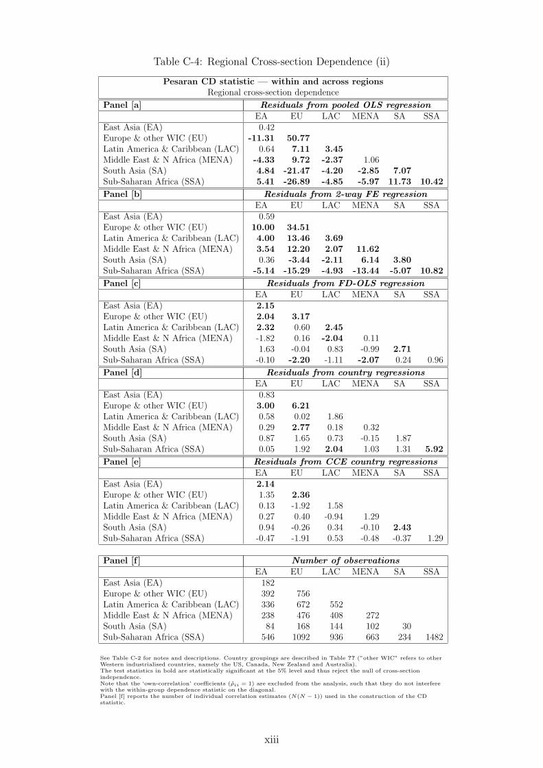
Table C-4: Regional Cross-section Dependence (ii)
Pesaran CD statistic — within and across regionsRegional cross-section dependence
Panel [a] Residuals from pooled OLS regressionEA EU LAC MENA SA SSA
East Asia (EA) 0.42Europe & other WIC (EU) -11.31 50.77Latin America & Caribbean (LAC) 0.64 7.11 3.45Middle East & N Africa (MENA) -4.33 9.72 -2.37 1.06South Asia (SA) 4.84 -21.47 -4.20 -2.85 7.07Sub-Saharan Africa (SSA) 5.41 -26.89 -4.85 -5.97 11.73 10.42
Panel [b] Residuals from 2-way FE regressionEA EU LAC MENA SA SSA
East Asia (EA) 0.59Europe & other WIC (EU) 10.00 34.51Latin America & Caribbean (LAC) 4.00 13.46 3.69Middle East & N Africa (MENA) 3.54 12.20 2.07 11.62South Asia (SA) 0.36 -3.44 -2.11 6.14 3.80Sub-Saharan Africa (SSA) -5.14 -15.29 -4.93 -13.44 -5.07 10.82
Panel [c] Residuals from FD-OLS regressionEA EU LAC MENA SA SSA
East Asia (EA) 2.15Europe & other WIC (EU) 2.04 3.17Latin America & Caribbean (LAC) 2.32 0.60 2.45Middle East & N Africa (MENA) -1.82 0.16 -2.04 0.11South Asia (SA) 1.63 -0.04 0.83 -0.99 2.71Sub-Saharan Africa (SSA) -0.10 -2.20 -1.11 -2.07 0.24 0.96
Panel [d] Residuals from country regressionsEA EU LAC MENA SA SSA
East Asia (EA) 0.83Europe & other WIC (EU) 3.00 6.21Latin America & Caribbean (LAC) 0.58 0.02 1.86Middle East & N Africa (MENA) 0.29 2.77 0.18 0.32South Asia (SA) 0.87 1.65 0.73 -0.15 1.87Sub-Saharan Africa (SSA) 0.05 1.92 2.04 1.03 1.31 5.92
Panel [e] Residuals from CCE country regressionsEA EU LAC MENA SA SSA
East Asia (EA) 2.14Europe & other WIC (EU) 1.35 2.36Latin America & Caribbean (LAC) 0.13 -1.92 1.58Middle East & N Africa (MENA) 0.27 0.40 -0.94 1.29South Asia (SA) 0.94 -0.26 0.34 -0.10 2.43Sub-Saharan Africa (SSA) -0.47 -1.91 0.53 -0.48 -0.37 1.29
Panel [f ] Number of observationsEA EU LAC MENA SA SSA
East Asia (EA) 182Europe & other WIC (EU) 392 756Latin America & Caribbean (LAC) 336 672 552Middle East & N Africa (MENA) 238 476 408 272South Asia (SA) 84 168 144 102 30Sub-Saharan Africa (SSA) 546 1092 936 663 234 1482
See Table C-2 for notes and descriptions. Country groupings are described in Table ?? (”other WIC” refers to otherWestern industrialised countries, namely the US, Canada, New Zealand and Australia).The test statistics in bold are statistically significant at the 5% level and thus reject the null of cross-sectionindependence.Note that the ‘own-correlation’ coefficients (ρii = 1) are excluded from the analysis, such that they do not interferewith the within-group dependence statistic on the diagonal.Panel [f] reports the number of individual correlation estimates (N(N − 1)) used in the construction of the CDstatistic.
xiii
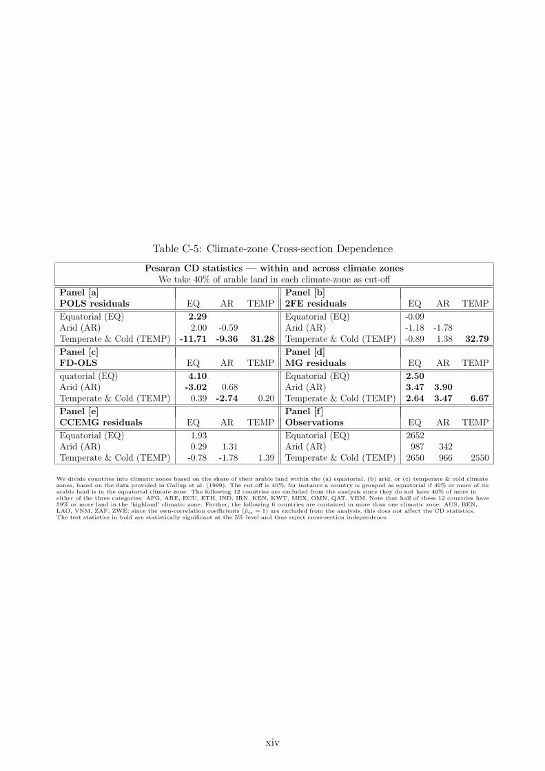
Table C-5: Climate-zone Cross-section Dependence
Pesaran CD statistics — within and across climate zonesWe take 40% of arable land in each climate-zone as cut-off
Panel [a] Panel [b]POLS residuals EQ AR TEMP 2FE residuals EQ AR TEMP
Equatorial (EQ) 2.29 Equatorial (EQ) -0.09Arid (AR) 2.00 -0.59 Arid (AR) -1.18 -1.78Temperate & Cold (TEMP) -11.71 -9.36 31.28 Temperate & Cold (TEMP) -0.89 1.38 32.79
Panel [c] Panel [d]FD-OLS EQ AR TEMP MG residuals EQ AR TEMP
quatorial (EQ) 4.10 Equatorial (EQ) 2.50Arid (AR) -3.02 0.68 Arid (AR) 3.47 3.90Temperate & Cold (TEMP) 0.39 -2.74 0.20 Temperate & Cold (TEMP) 2.64 3.47 6.67
Panel [e] Panel [f ]CCEMG residuals EQ AR TEMP Observations EQ AR TEMP
Equatorial (EQ) 1.93 Equatorial (EQ) 2652Arid (AR) 0.29 1.31 Arid (AR) 987 342Temperate & Cold (TEMP) -0.78 -1.78 1.39 Temperate & Cold (TEMP) 2650 966 2550
We divide countries into climatic zones based on the share of their arable land within the (a) equatorial, (b) arid, or (c) temperate & cold climatezones, based on the data provided in Gallup et al. (1999). The cut-off is 40%; for instance a country is grouped as equatorial if 40% or more of itsarable land is in the equatorial climate zone. The following 12 countries are excluded from the analysis since they do not have 40% of more ineither of the three categories: AFG, ARE, ECU, ETH, IND, IRN, KEN, KWT, MEX, OMN, QAT, YEM. Note that half of these 12 countries have59% or more land in the ‘highland’ climatic zone. Further, the following 6 countries are contained in more than one climatic zone: AUS, BEN,LAO, VNM, ZAF, ZWE; since the own-correlation coefficients (ρii = 1) are excluded from the analysis, this does not affect the CD statistics.The test statistics in bold are statistically significant at the 5% level and thus reject cross-section independence.
xiv

D Additional tables and figures
Table D-1: Dynamic specification — Pooled regressions (CRS imposed)
Pooled regressionsdependent variable: [1],[2] & [4]-[7] log output per worker, [3] dto. in 2FE transformation\,
[8] ∆log output per worker, [9] dto. in 2FE transformation\
[1] [2] [3] [4] [5] [6]POLS♦ 2FE\ CCEP CCEP CCEP CCEP
weight matrix‡ none neighbour distance agro-climate
lagged levels
output pw (t− 1) -0.0189 -0.1764 -0.6072 -0.4024 -0.4959 -0.5699[5.71]∗∗ [22.80]∗∗ [22.54]∗∗ [19.87]∗∗ [21.44]∗∗ [22.80]∗∗
tractors pw (t− 1) 0.0022 0.0134 0.0678 0.0454 0.0429 0.0493[1.85] [5.47]∗∗ [7.02]∗∗ [7.51]∗∗ [5.90]∗∗ [5.76]∗∗
livestock pw (t− 1) 0.0042 0.0709 0.2045 0.1064 0.1850 0.2298[2.49]∗ [10.07]∗∗ [9.67]∗∗ [5.89]∗∗ [9.31]∗∗ [10.32]∗∗
fertilizer pw (t− 1) 0.0061 0.0147 0.0258 0.0360 0.0243 0.0237[5.86]∗∗ [7.76]∗∗ [5.79]∗∗ [8.45]∗∗ [4.10]∗∗ [5.64]∗∗
land pw (t− 1) 0.0045 0.0554 0.1959 0.1097 0.1980 0.1837[2.28]∗ [7.28]∗∗ [5.35]∗∗ [4.46]∗∗ [6.38]∗∗ [5.77]∗∗
growth rates
∆tractors pw 0.0555 0.0970 0.0828 0.0591 0.0558 0.0771[4.12]∗∗ [8.49]∗∗ [4.37]∗∗ [3.55]∗∗ [4.61]∗∗ [4.82]∗∗
∆livestock pw 0.3153 0.3307 0.3097 0.2899 0.3175 0.2726[7.57]∗∗ [17.31]∗∗ [9.43]∗∗ [8.82]∗∗ [10.65]∗∗ [8.21]∗∗
∆fertilizer pw 0.0123 0.0172 0.0132 0.0196 0.0171 0.0152[3.48]∗∗ [5.63]∗∗ [3.27]∗∗ [4.79]∗∗ [3.67]∗∗ [3.99]∗∗
∆land pw 0.3010 0.3290 0.3249 0.3272 0.3404 0.3170[4.38]∗∗ [11.67]∗∗ [4.86]∗∗ [5.88]∗∗ [7.42]∗∗ [6.42]∗∗
Constant 0.0485 2.6725 1.7939 0.0141 3.5301[5.34]∗∗ [0.35] [1.75] [0.01] [1.85]
Observations 5,013 5,013 5,013 5,013 5,013 5,013R-squared 0.12 0.20 0.54 0.54 0.81 0.60
Estimated long-run coefficients[
tractors pw 0.118 0.076 0.112 0.113 0.087 0.087[2.09]∗ [5.58]∗∗ [7.21]∗∗ [7.73]∗∗ [6.33]∗∗ [5.80]∗∗
livestock pw 0.224 0.402 0.337 0.264 0.373 0.403[2.77]∗∗ [11.30]∗∗ [10.51]∗∗ [6.30]∗∗ [10.40]∗∗ [11.27]∗∗
fertilizer pw 0.322 0.083 0.042 0.089 0.049 0.042[5.07]∗∗ [8.09]∗∗ [5.85]∗∗ [8.67]∗∗ [4.16]∗∗ [5.80]∗∗
land pw 0.238 0.314 0.323 0.273 0.399 0.322[2.56]∗ [7.95]∗∗ [5.34]∗∗ [4.50]∗∗ [6.69]∗∗ [5.93]∗∗
Implied βL 0.098 0.125 0.186 0.261 0.092 0.146
Arellano-Bond Serial Correlation Test — H0: no serial correlation in the residuals
AR(1) (p) -9.69 (.00) -14.95 (.00) -3.30 (.00) -6.46 (.00) -4.71 (.00) -3.88 (.00)AR(2) (p) -0.41 (.68) 3.15 (.00) -1.28 (.20) 1.43 (.15) -3.36 (.00) 0.06 (.95)AR(3) (p) 0.60 (.55) 4.12 (.00) -1.68 (.09) 0.39 (.70) -0.82 (.41) -1.98 (.05)
Nonstationarity: Pesaran (2007) CIPS test applied to residuals] — H0: residuals are I(1)
lags Ztbar (p) Ztbar (p) Ztbar (p) Ztbar (p) Ztbar (p) Ztbar (p)none -48.93 (.00) -44.51 (.00) -45.04 (.00) -47.06 (.00) -45.84 (.00) -44.61 (.00)1 lag -38.33 (.00) -29.68 (.00) -32.18 (.00) -32.43 (.00) -32.08 (.00) -31.67 (.00)2 lags -23.23 (.00) -16.08 (.00) -20.66 (.00) -21.58 (.00) -22.27 (.00) -20.41 (.00)3 lags -15.77 (.00) -8.30 (.00) -16.05 (.00) -14.15 (.00) -16.51 (.00) -15.44 (.00)
CSD: Mean Correlation coefficient & Pesaran (2004) CD test — H0: no CSD
Mean ρij 0.00 0.01 0.00 0.00 0.10 0.00Mean |ρij| 0.14 0.15 0.17 0.14 0.16 0.15CD (p) -0.08 (.94) 2.66 (.00) -0.47 (.64) 1.31 (.19) 26.34 (.00) -0.62 (.53)
Further residual diagnostic tests? — H0: no heteroskedasticity, regular skewness/kurtosis
(A) Joint testχ2 (p) 1019.7 (.00) 943.6 (.00) 623.4 (.00) 551.0 (.00) 559.4 (.00) 566.1 (.00)
(B) Joint testχ2 (p) 1463.7 (.00) 1166.1 (.00) - - - -
Notes: See Table 6 for details.♦ We include T − 1 year dummies in equation [1].
xv