Neil W. Polhemus, CTO, StatPoint Technologies, Inc.

Multivariate Data Analysis

Using Statgraphics Centurion:

Part 1

Copyright 2013 by StatPoint Technologies, Inc.

Web site: www.statgraphics.com

Multivariate Statistical Methods

The simultaneous observation and analysis of more than one

response variable.

*Primary Uses

1. Data reduction or structural simplification

2. Sorting and grouping

3. Investigation of the dependence among variables

4. Prediction

5. Hypothesis construction and testing

*Johnson and Wichern, Applied Multivariate Statistical Analysis

2

STATGRAPHICS Contents

Plot – Multivariate Visualization

Scatterplot matrix

Parallel coordinates plot

Andrews plot

Star glyphs and sunray plots

Chernoff faces

Describe – Multivariate Methods Correlation analysis

Principal components analysis

Factor analysis

Canonical correlations

Cluster analysis

Correspondence analysis

Multiple correspondence analysis 3

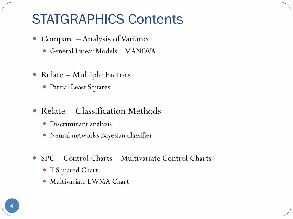
STATGRAPHICS Contents

Compare – Analysis of Variance

General Linear Models – MANOVA

Relate – Multiple Factors

Partial Least Squares

Relate – Classification Methods Discriminant analysis

Neural networks Bayesian classifier

SPC – Control Charts – Multivariate Control Charts

T-Squared Chart

Multivariate EWMA Chart

4

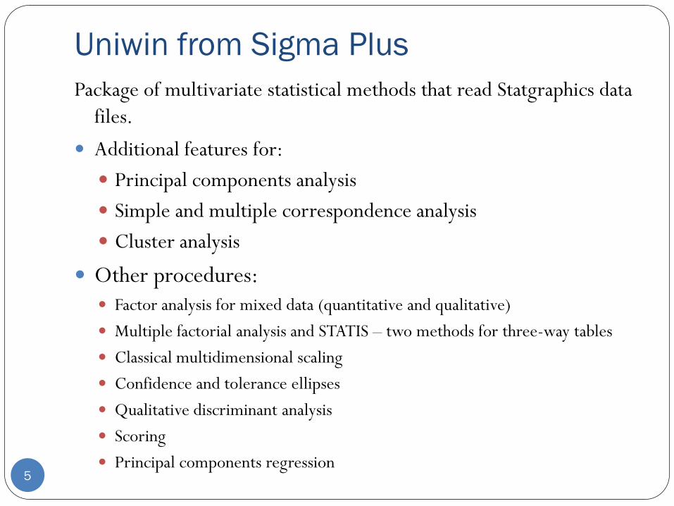
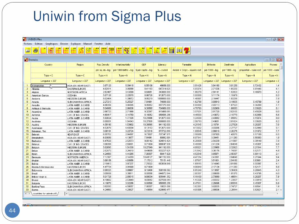
Uniwin from Sigma Plus

Package of multivariate statistical methods that read Statgraphics data

files.

Additional features for:

Principal components analysis

Simple and multiple correspondence analysis

Cluster analysis

Other procedures: Factor analysis for mixed data (quantitative and qualitative)

Multiple factorial analysis and STATIS – two methods for three-way tables

Classical multidimensional scaling

Confidence and tolerance ellipses

Qualitative discriminant analysis

Scoring

Principal components regression 5

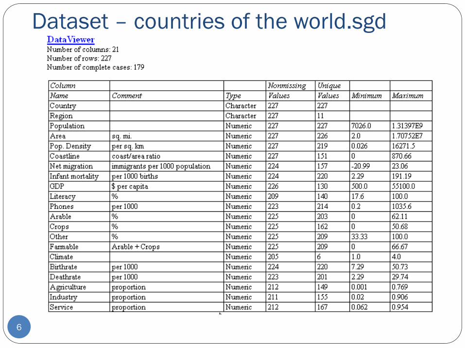
Dataset – countries of the world.sgd

6

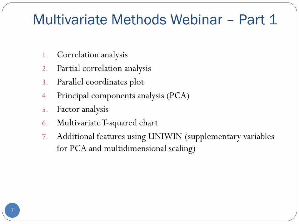
Multivariate Methods Webinar – Part 1

1. Correlation analysis

2. Partial correlation analysis

3. Parallel coordinates plot

4. Principal components analysis (PCA)

5. Factor analysis

6. Multivariate T-squared chart

7. Additional features using UNIWIN (supplementary variables

for PCA and multidimensional scaling)

7

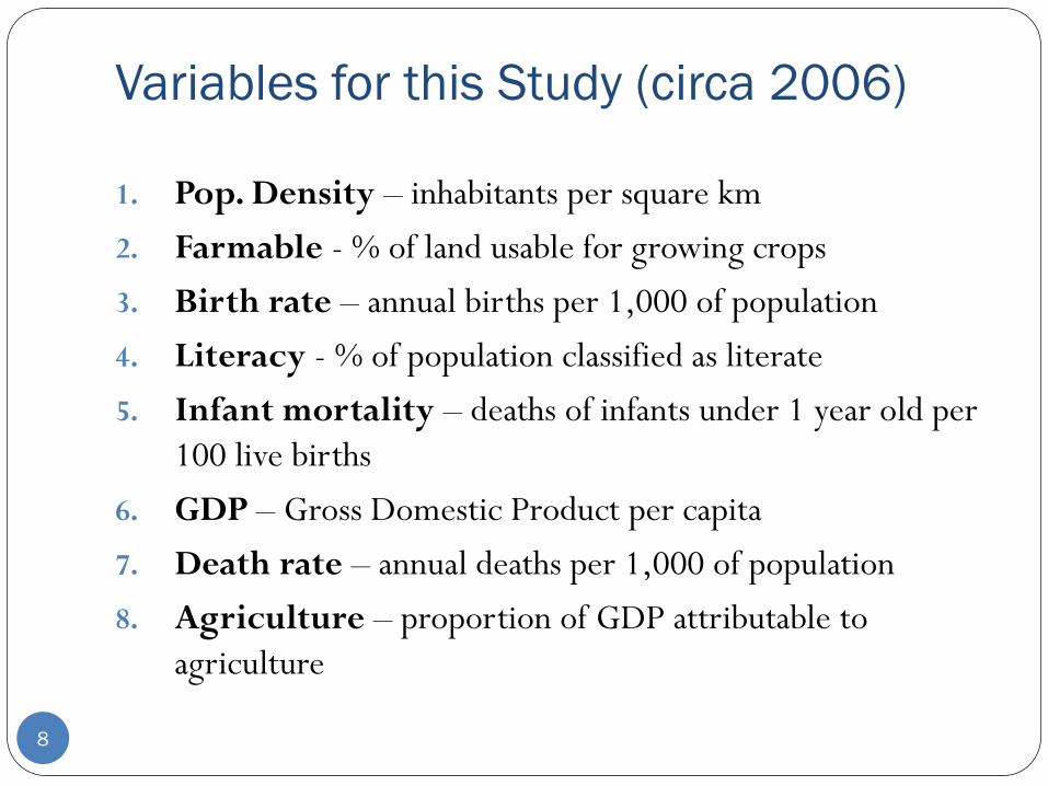
Variables for this Study (circa 2006)

1. Pop. Density – inhabitants per square km

2. Farmable - % of land usable for growing crops

3. Birth rate – annual births per 1,000 of population

4. Literacy - % of population classified as literate

5. Infant mortality – deaths of infants under 1 year old per

100 live births

6. GDP – Gross Domestic Product per capita

7. Death rate – annual deaths per 1,000 of population

8. Agriculture – proportion of GDP attributable to

agriculture

8

Matrix Plot – gives initial view of the data

9

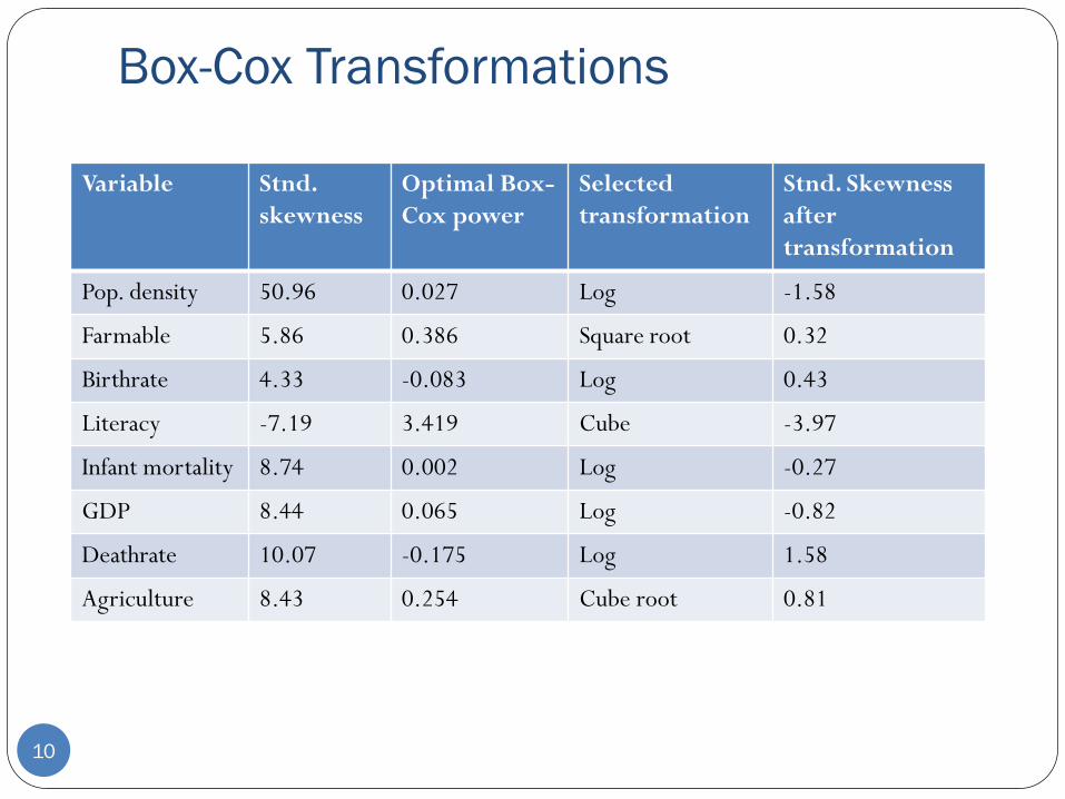
Box-Cox Transformations

10

Variable Stnd.

skewness

Optimal Box-

Cox power

Selected

transformation

Stnd. Skewness

after

transformation

Pop. density 50.96 0.027 Log -1.58

Farmable 5.86 0.386 Square root 0.32

Birthrate 4.33 -0.083 Log 0.43

Literacy -7.19 3.419 Cube -3.97

Infant mortality 8.74 0.002 Log -0.27

GDP 8.44 0.065 Log -0.82

Deathrate 10.07 -0.175 Log 1.58

Agriculture 8.43 0.254 Cube root 0.81

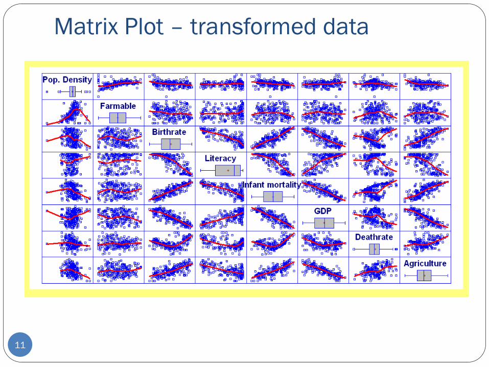
Matrix Plot – transformed data

11

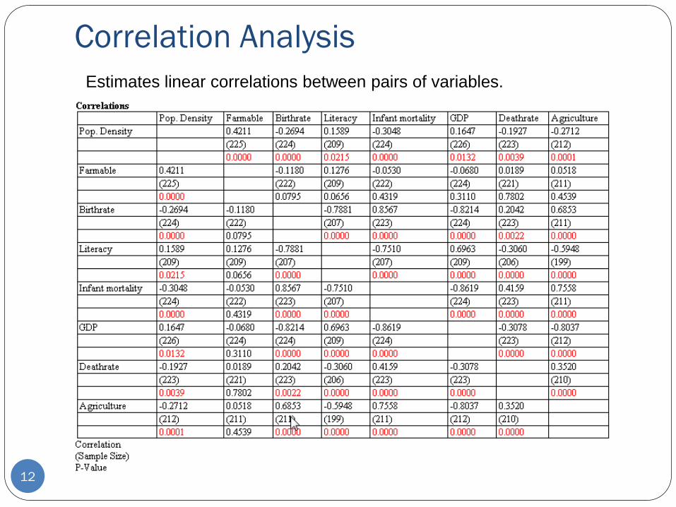
Correlation Analysis

12

Estimates linear correlations between pairs of variables.

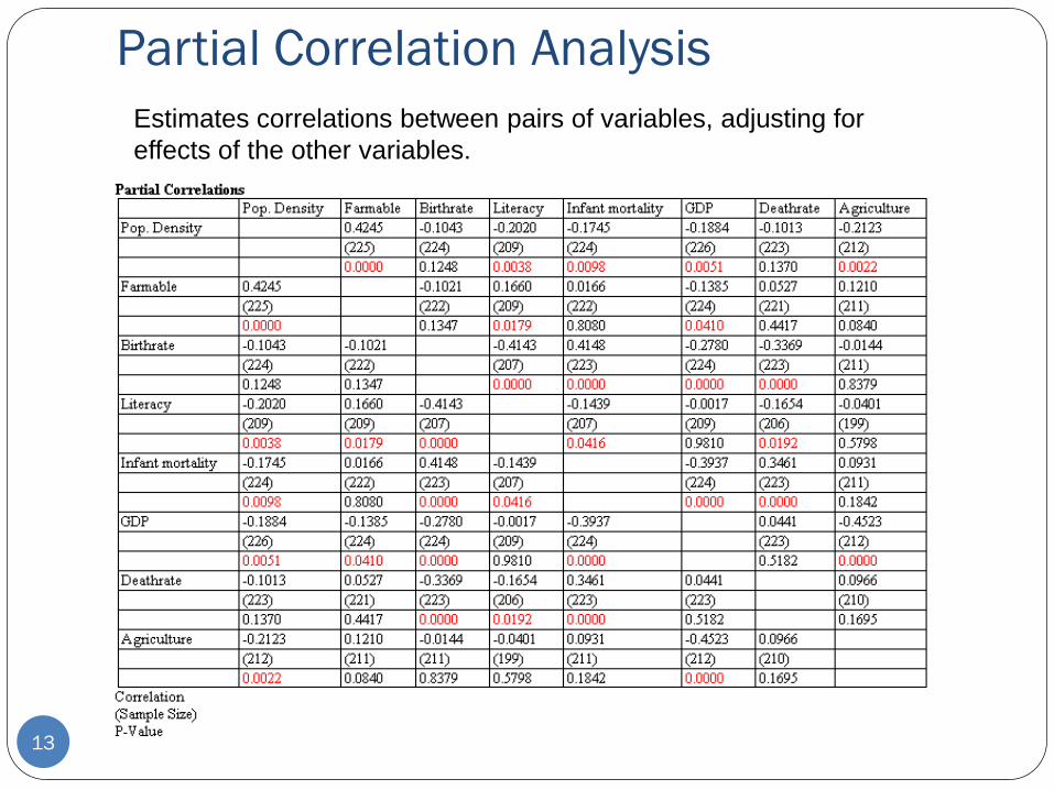
Partial Correlation Analysis

13

Estimates correlations between pairs of variables, adjusting for

effects of the other variables.

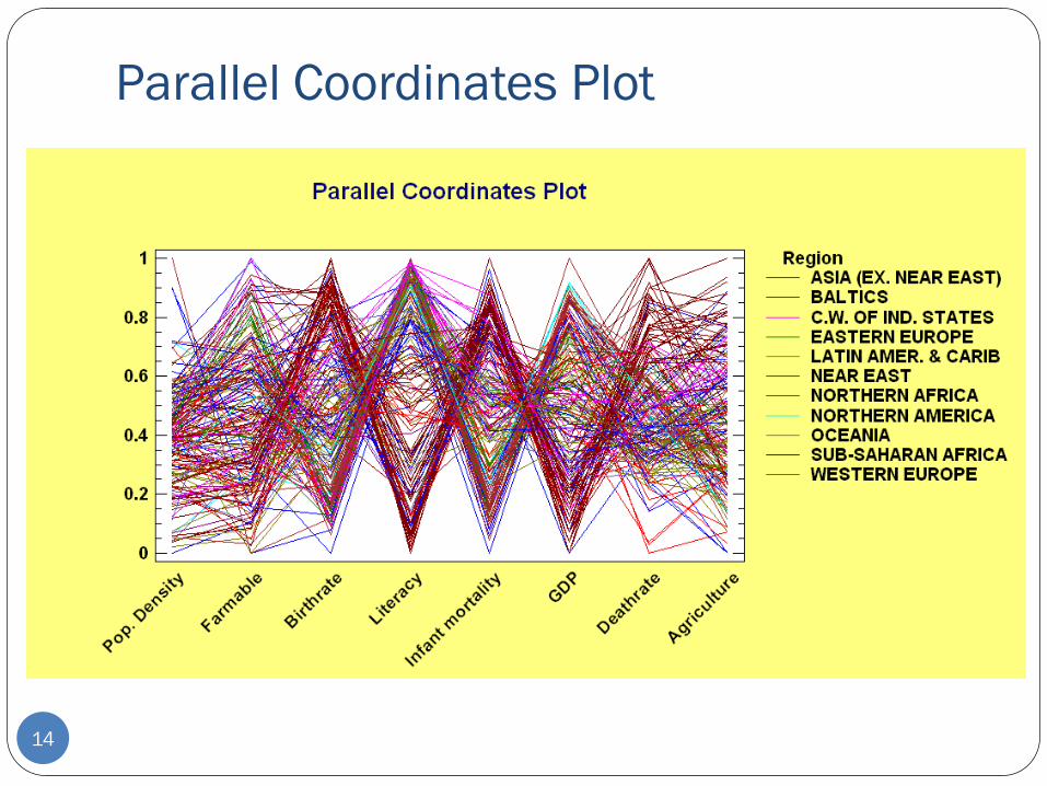
Parallel Coordinates Plot

14

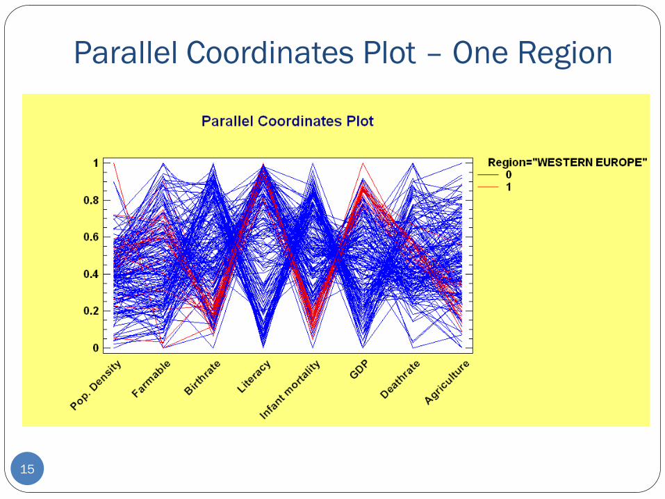
Parallel Coordinates Plot – One Region

15

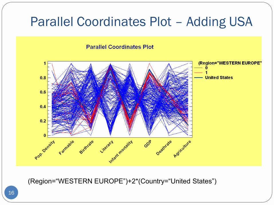
Parallel Coordinates Plot – Adding USA

16

(Region=“WESTERN EUROPE”)+2*(Country=“United States”)

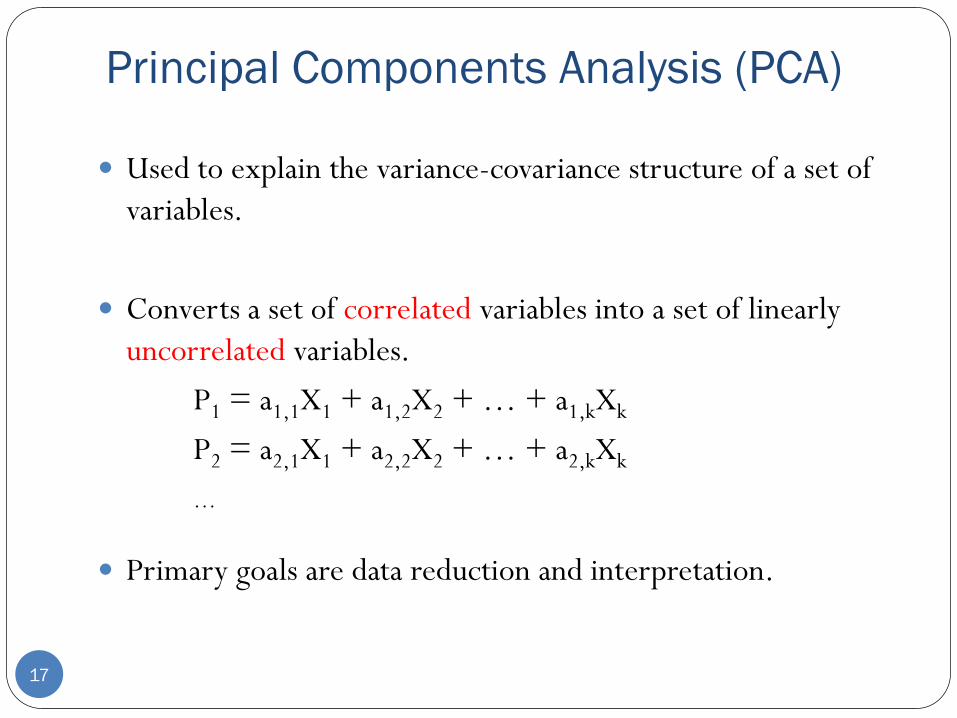
Principal Components Analysis (PCA)

Used to explain the variance-covariance structure of a set of

variables.

Converts a set of correlated variables into a set of linearly

uncorrelated variables.

P1 = a1,1X1 + a1,2X2 + … + a1,kXk

P2 = a2,1X1 + a2,2X2 + … + a2,kXk

…

Primary goals are data reduction and interpretation.

17

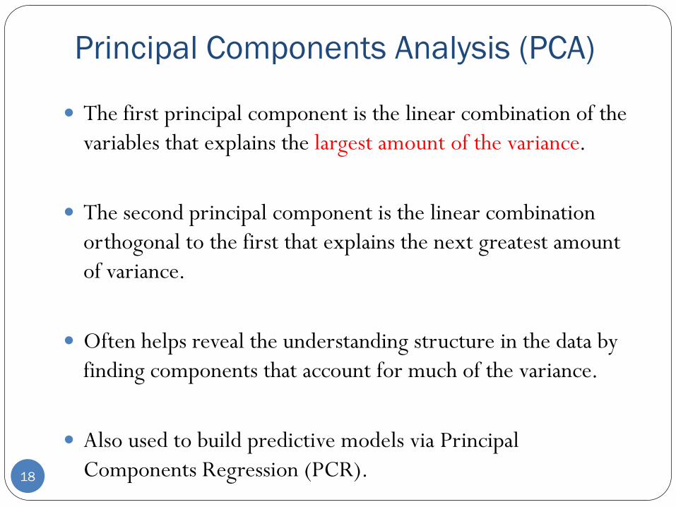
Principal Components Analysis (PCA)

The first principal component is the linear combination of the

variables that explains the largest amount of the variance.

The second principal component is the linear combination

orthogonal to the first that explains the next greatest amount

of variance.

Often helps reveal the understanding structure in the data by

finding components that account for much of the variance.

Also used to build predictive models via Principal

Components Regression (PCR).

18

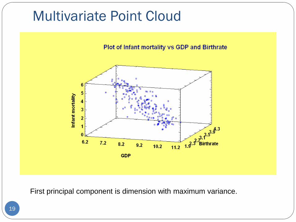
Multivariate Point Cloud

19

First principal component is dimension with maximum variance.

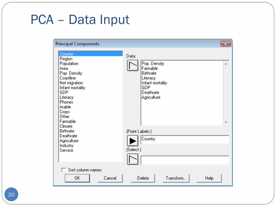
PCA – Data Input

20

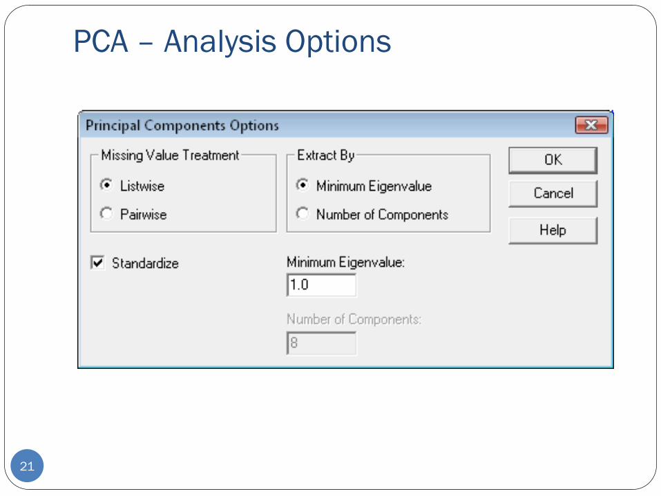
PCA – Analysis Options

21

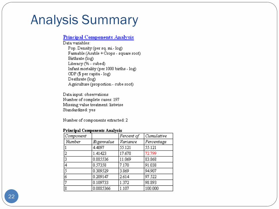
Analysis Summary

22

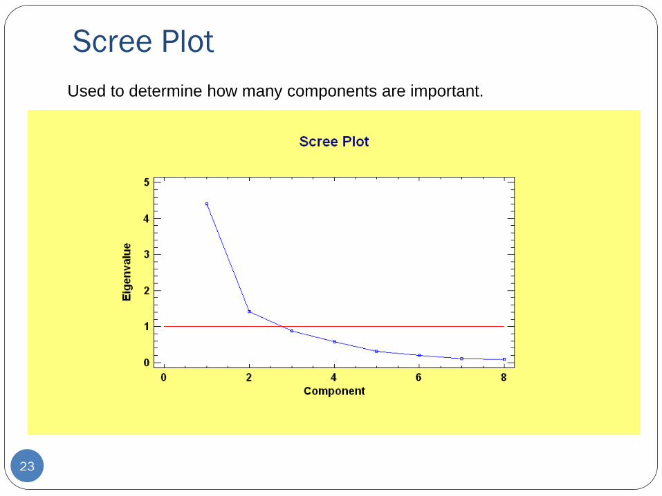
Scree Plot

23

Used to determine how many components are important.

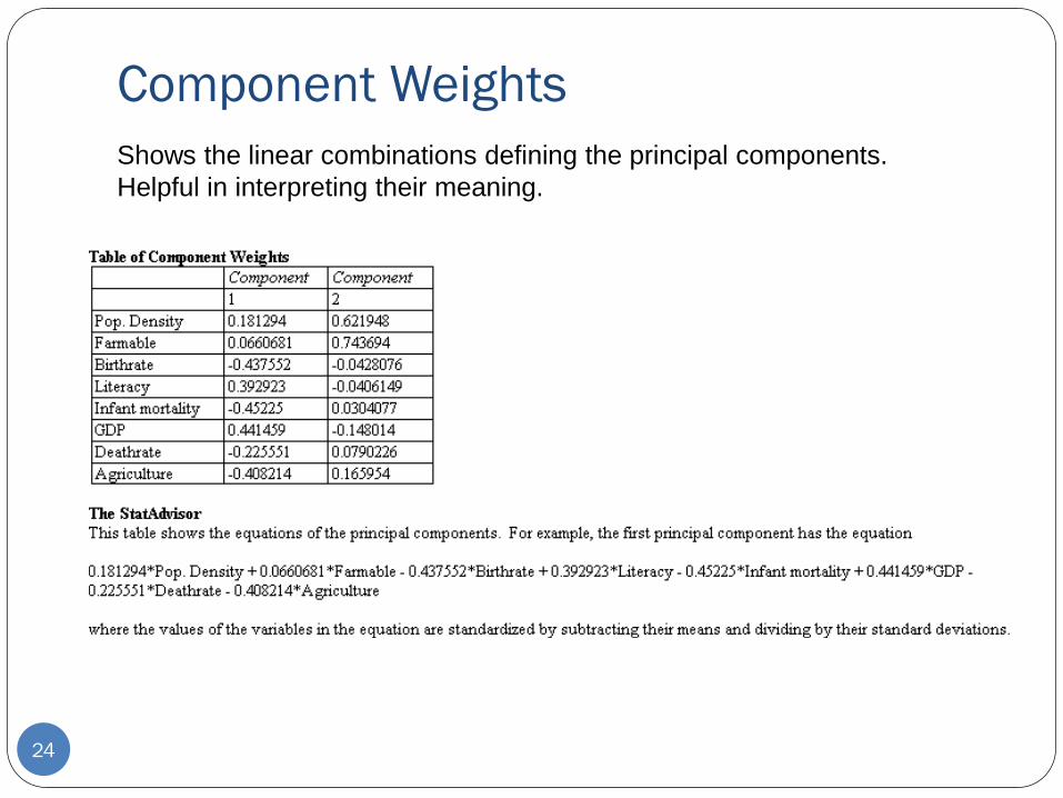
Component Weights

24

Shows the linear combinations defining the principal components.

Helpful in interpreting their meaning.

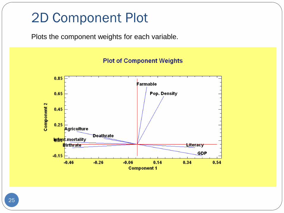
2D Component Plot

25

Plots the component weights for each variable.

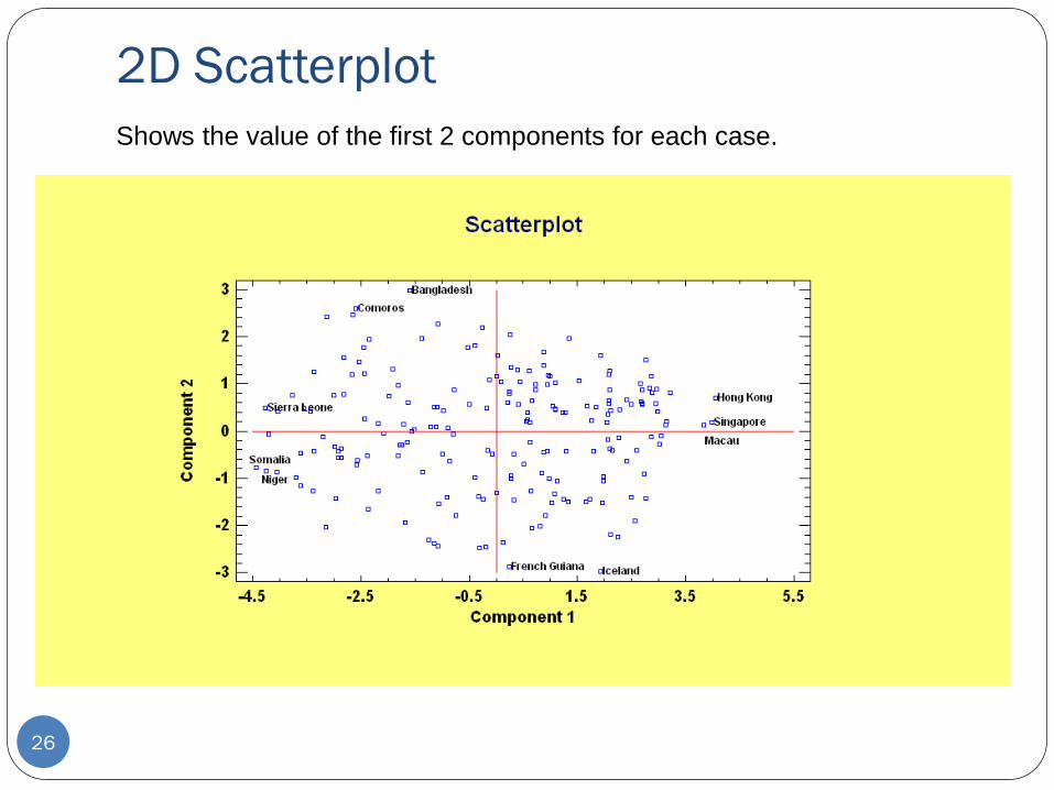
2D Scatterplot

26

Shows the value of the first 2 components for each case.

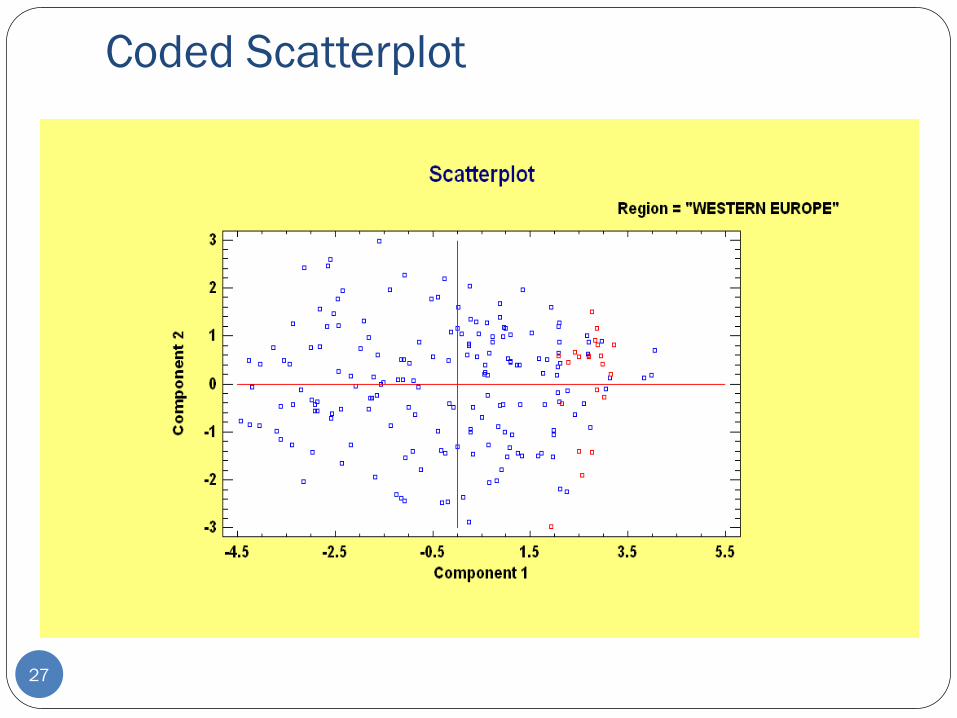
Coded Scatterplot

27

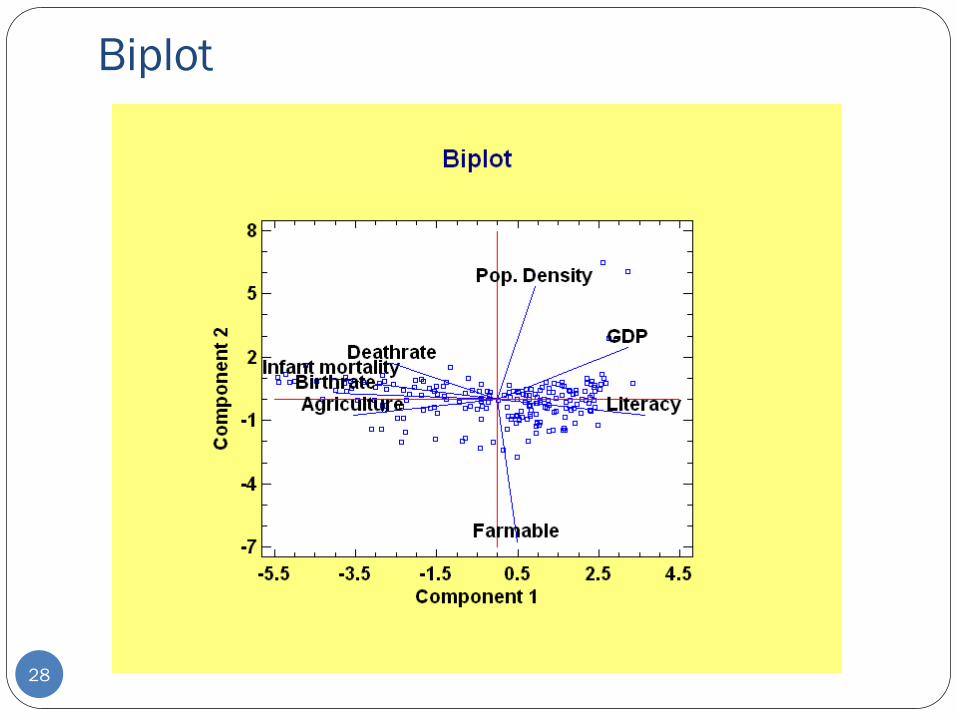
Biplot

28

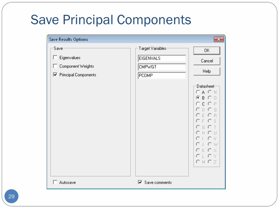
Save Principal Components

29

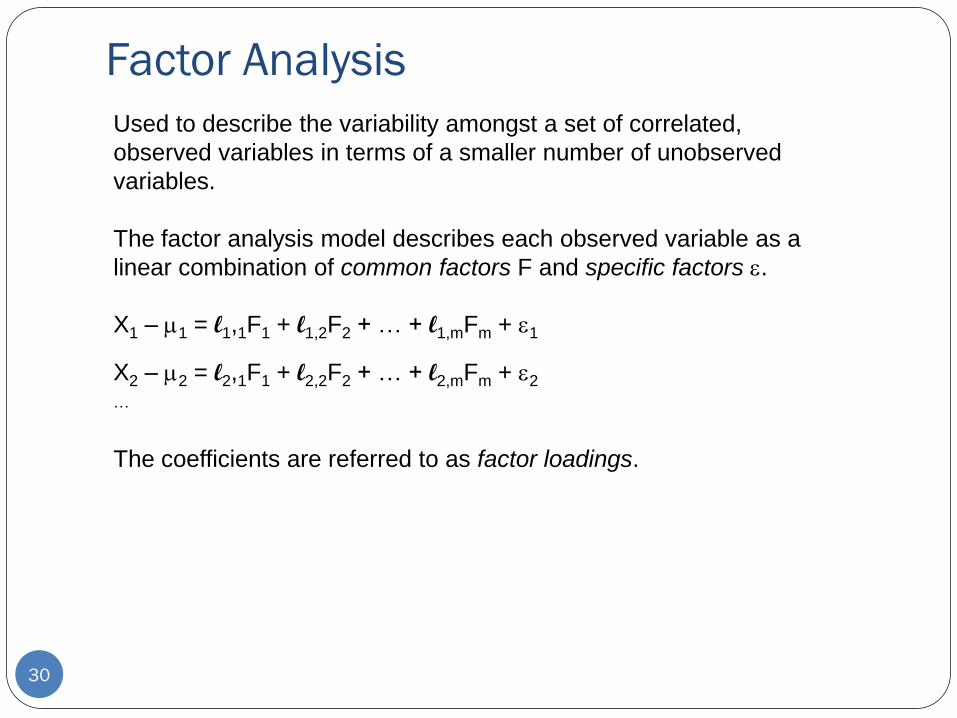
Factor Analysis

30

Used to describe the variability amongst a set of correlated,

observed variables in terms of a smaller number of unobserved

variables.

The factor analysis model describes each observed variable as a

linear combination of common factors F and specific factors e.

X1 – m1 = l1,1F1 + l1,2F2 + … + l1,mFm + e1

X2 – m2 = l2,1F1 + l2,2F2 + … + l2,mFm + e2

…

The coefficients are referred to as factor loadings.

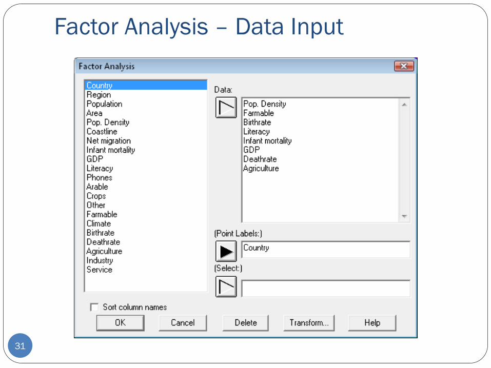
Factor Analysis – Data Input

31

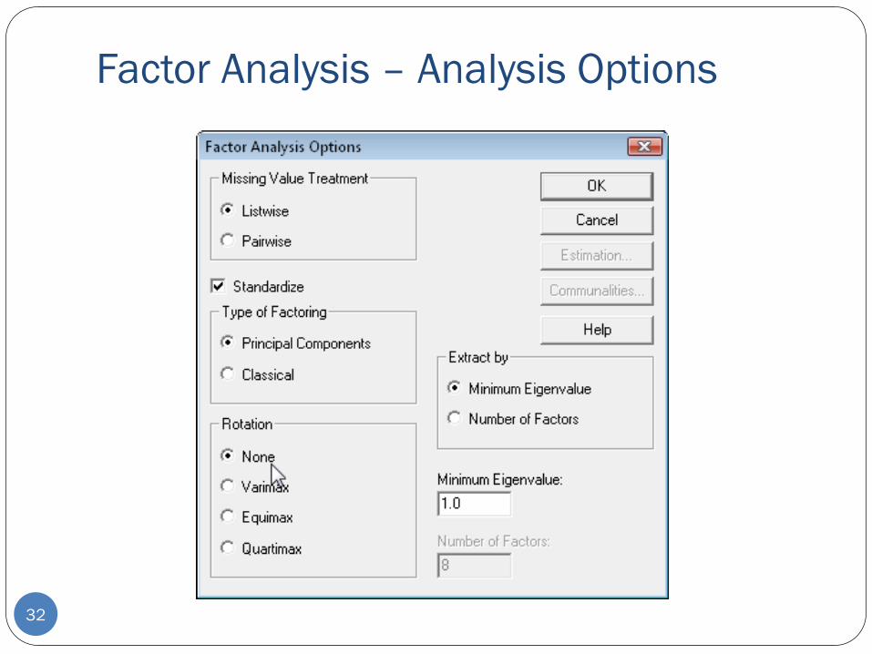
Factor Analysis – Analysis Options

32

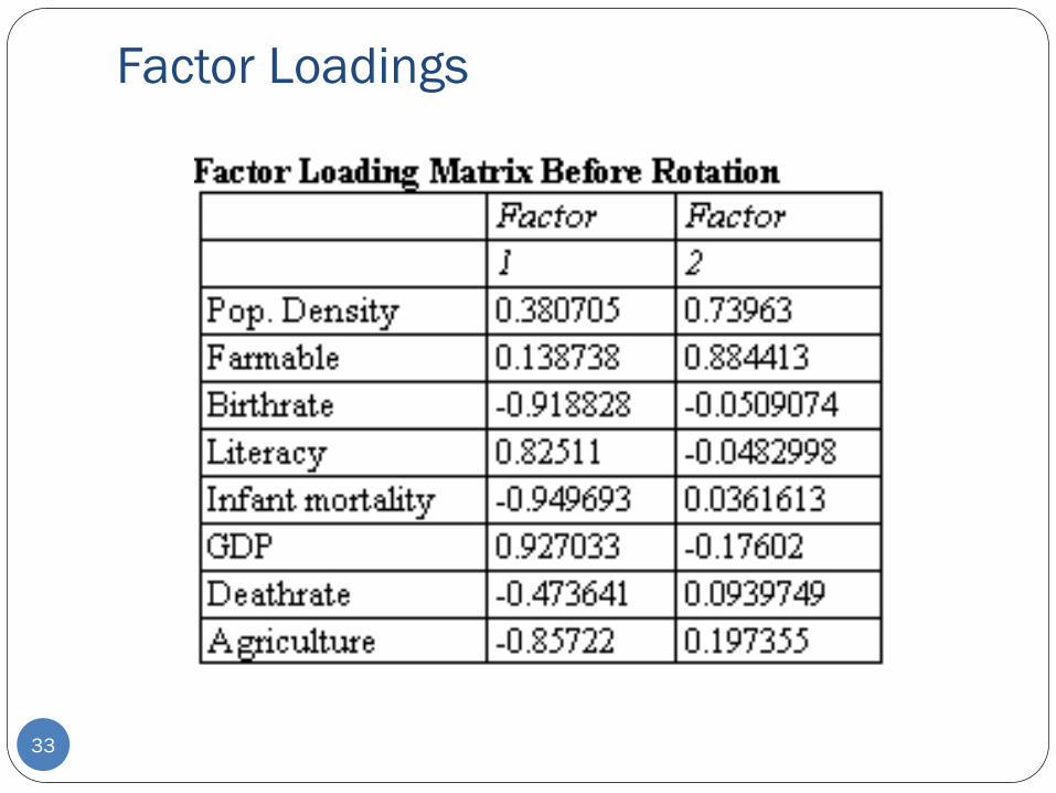
Factor Loadings

33

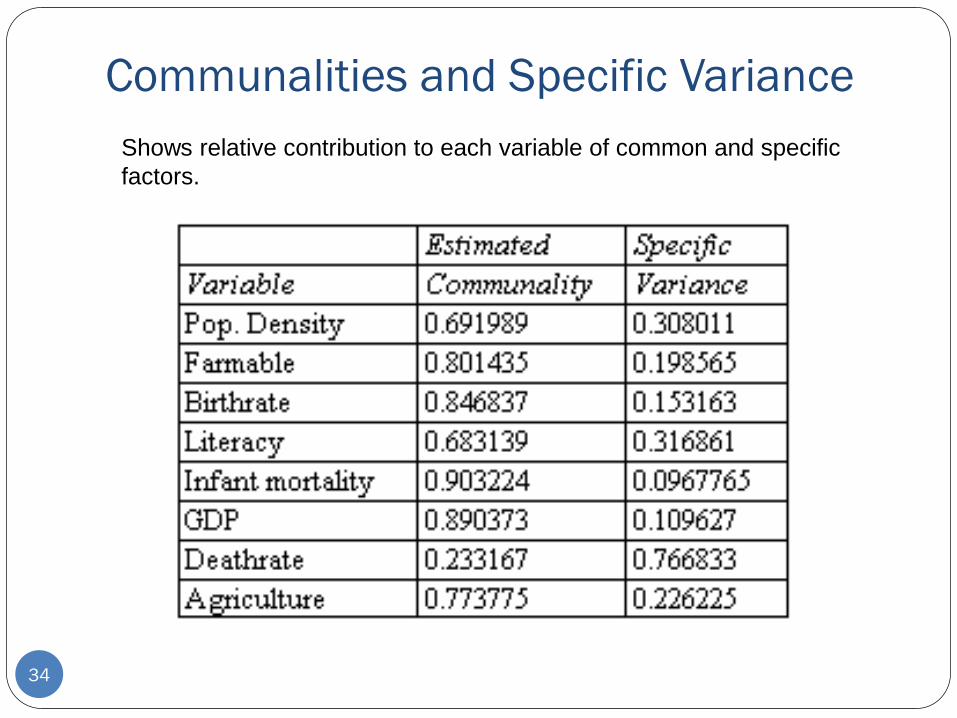
Communalities and Specific Variance

34

Shows relative contribution to each variable of common and specific

factors.

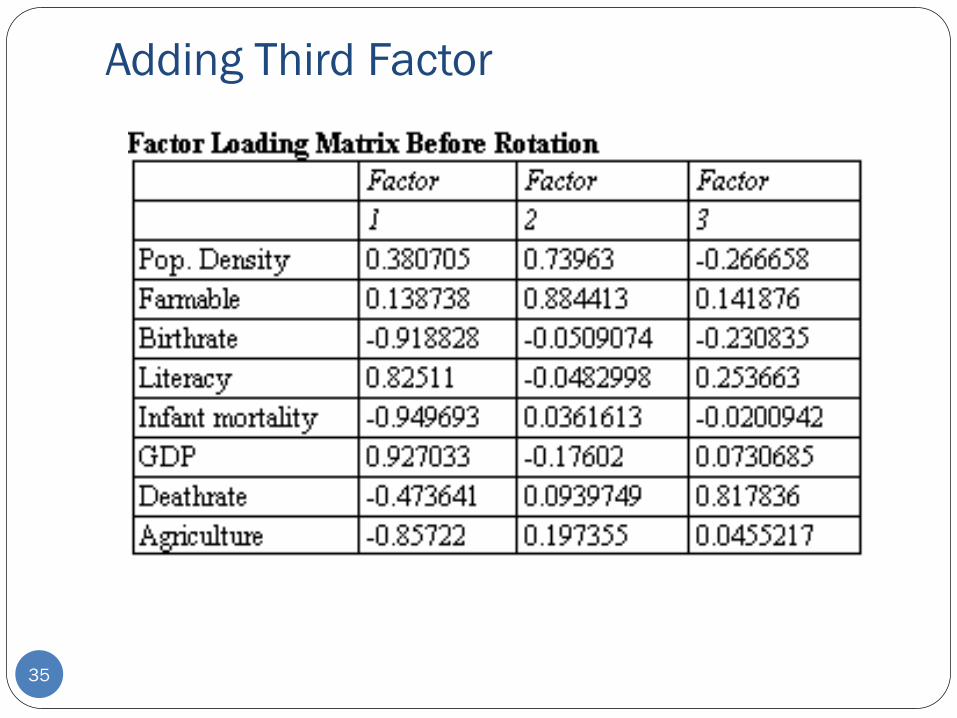
Adding Third Factor

35

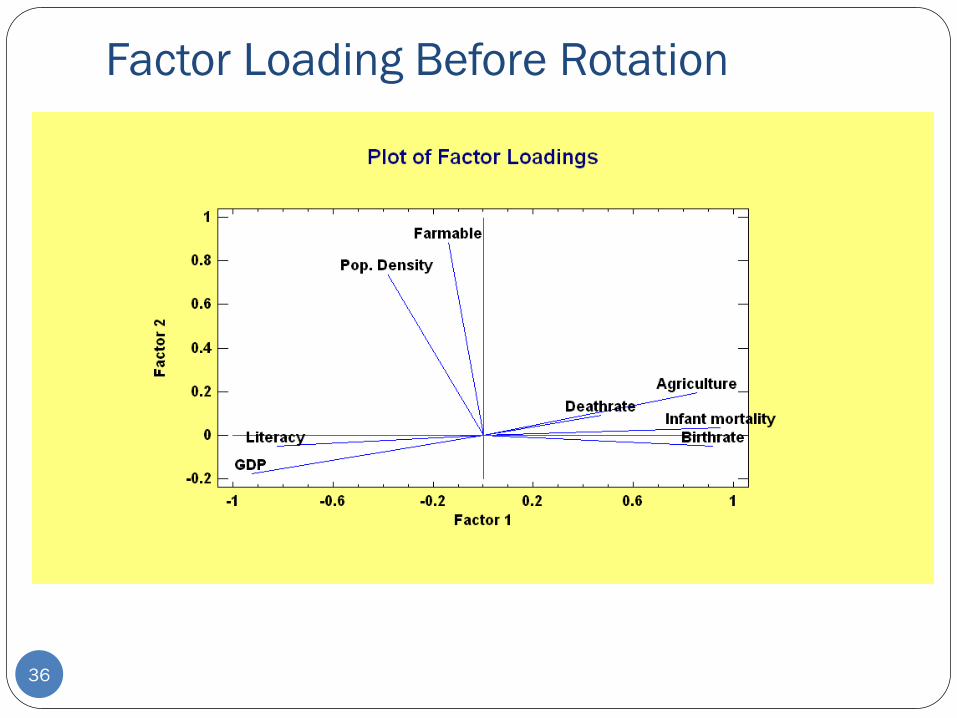
Factor Loading Before Rotation

36

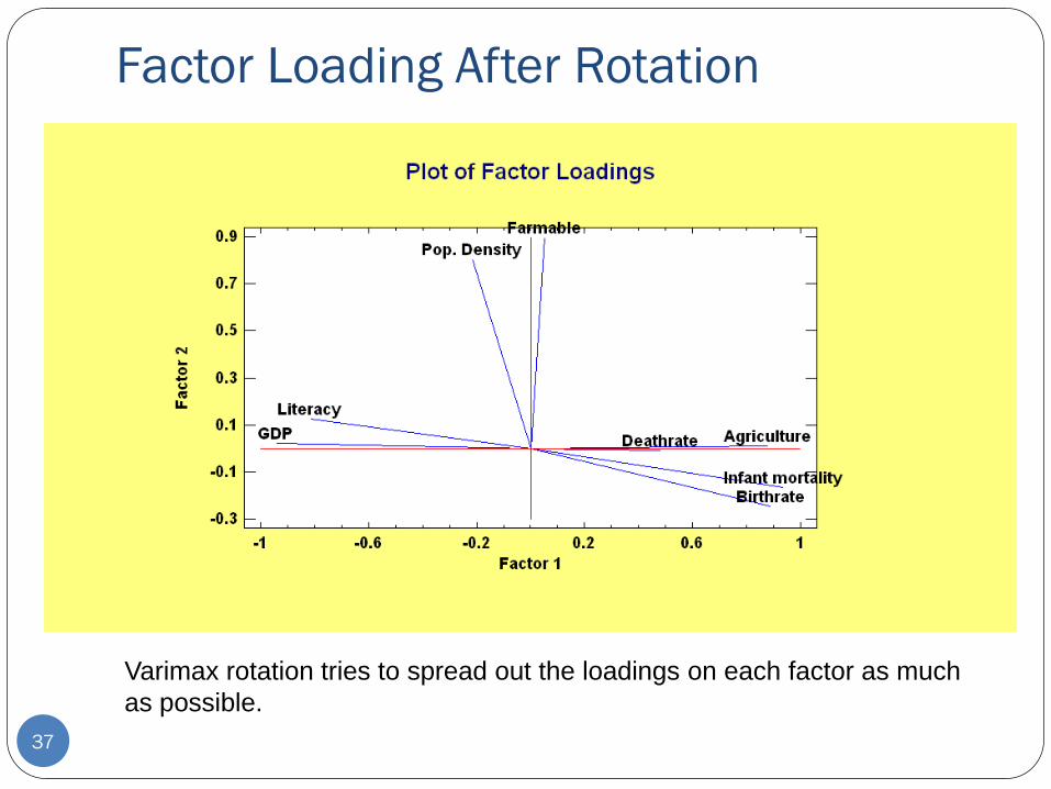
Factor Loading After Rotation

37

Varimax rotation tries to spread out the loadings on each factor as much

as possible.

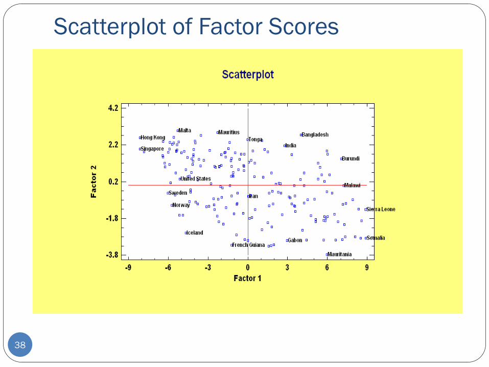
Scatterplot of Factor Scores

38

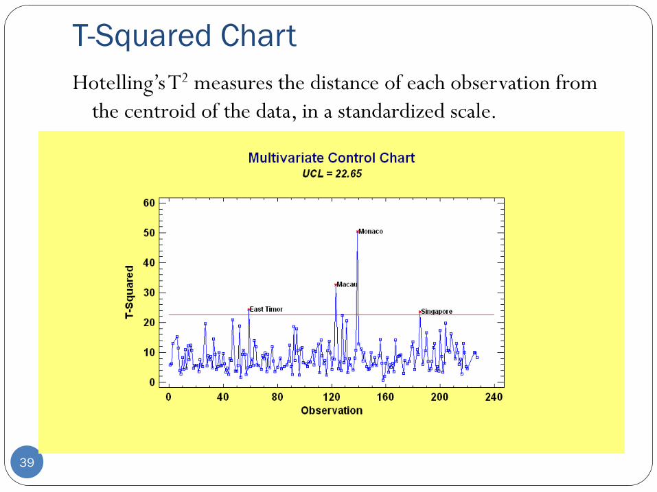
T-Squared Chart

Hotelling’s T2 measures the distance of each observation from

the centroid of the data, in a standardized scale.

39

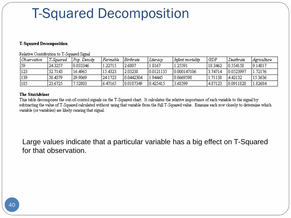
T-Squared Decomposition

40

Large values indicate that a particular variable has a big effect on T-Squared

for that observation.

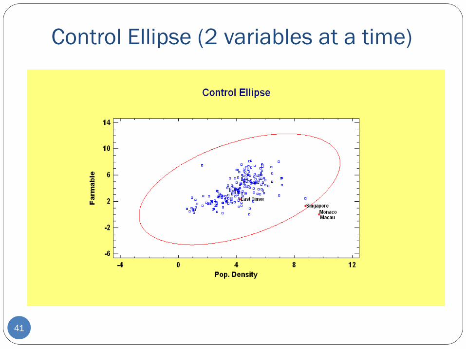
Control Ellipse (2 variables at a time)

41

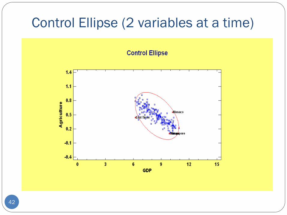
Control Ellipse (2 variables at a time)

42

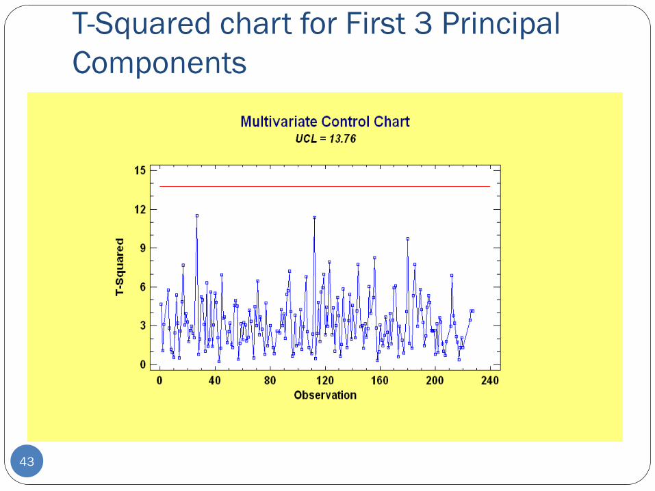
T-Squared chart for First 3 Principal

Components

43

Uniwin from Sigma Plus

44

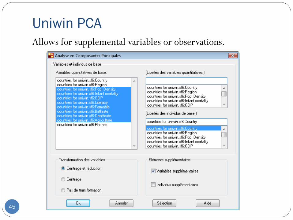
Uniwin PCA

Allows for supplemental variables or observations.

45

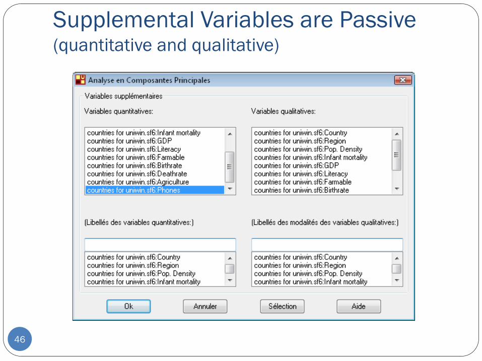
Supplemental Variables are Passive (quantitative and qualitative)

46

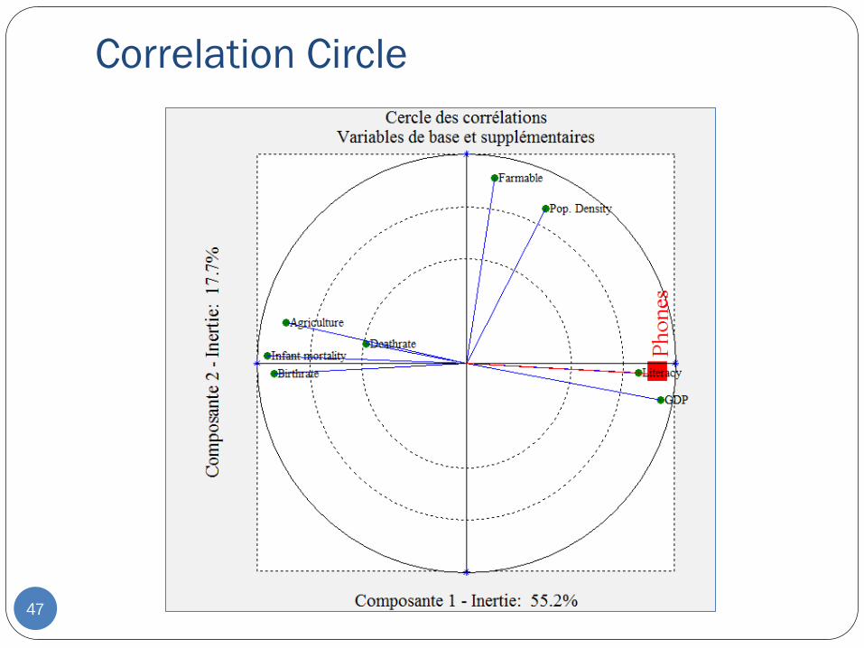
Correlation Circle

47

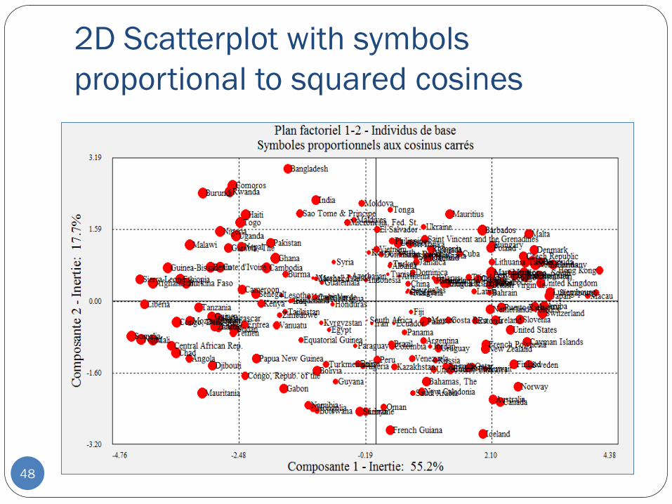
2D Scatterplot with symbols

proportional to squared cosines

48

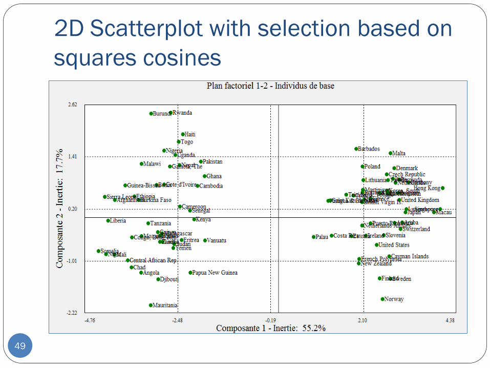
2D Scatterplot with selection based on

squares cosines

49

Multidimensional Scaling (Uniwin)

Objective: to display the observations in a low dimensional

coordinate system such that the distance between data points

is distorted as little as possible.

Input: an N by N matrix of similarities (or dissimilarities).

Output: a map displaying the location of the points in 2

dimensions.

50

Preparing a New Data File

Step 1: removed all rows with incomplete data on the 8

variables of interest.

Step 2: used the STANDARDIZE operator to subtract the mean

of each column and divide by its standard deviation.

Step 3: saved a new data file named “countries scaled for

UNIWIN.sf6”.

51

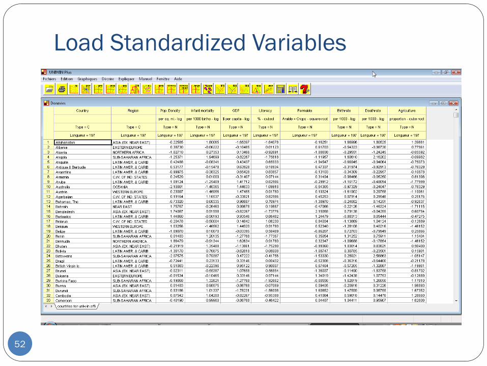
Load Standardized Variables

52

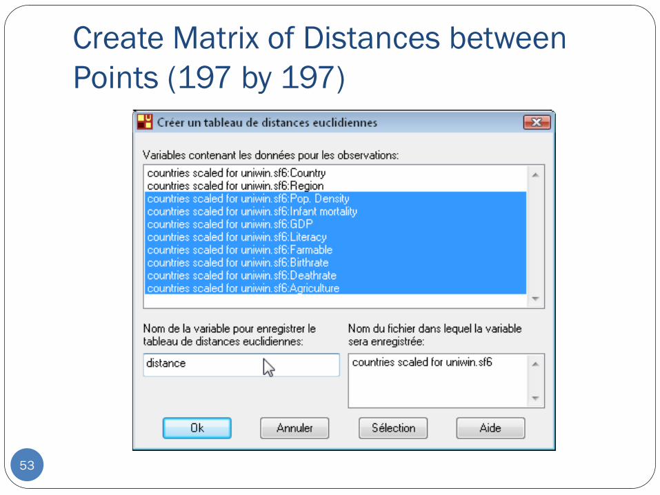
Create Matrix of Distances between

Points (197 by 197)

53

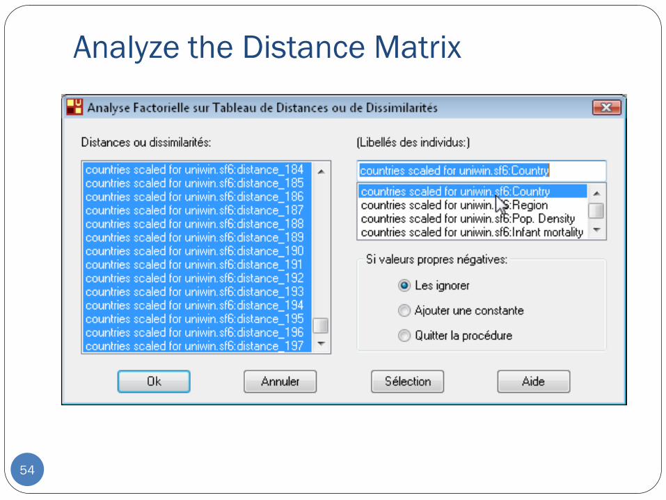
Analyze the Distance Matrix

54

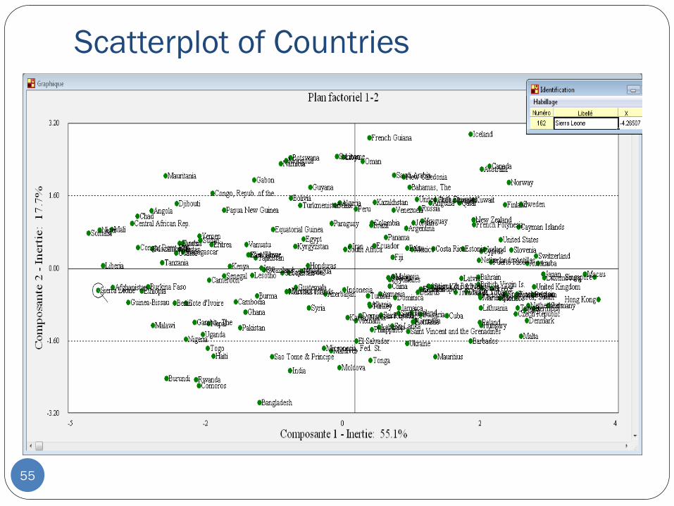
Scatterplot of Countries

55

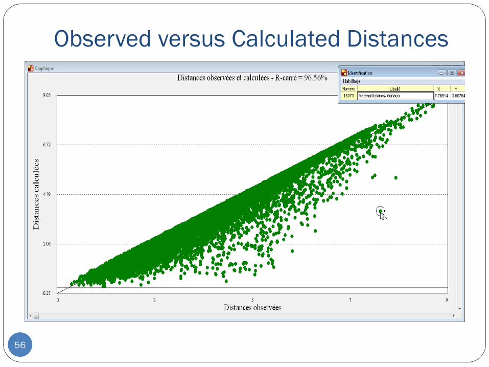
Observed versus Calculated Distances

56

More Information

57

Statgraphics Centurion: www.statgraphics.com

Uniwin: www.statgraphics.fr or www.sigmaplus.fr

Or send e-mail to info@statgraphics.com

Join the Statgraphics Community on:

Follow us on