Multivariate Co integration & Granger Causality under VECM ... · PDF fileMacroeconomic Variables on Inflation Dynamics in Bangladesh ... Granger causality under VECM. Getting data

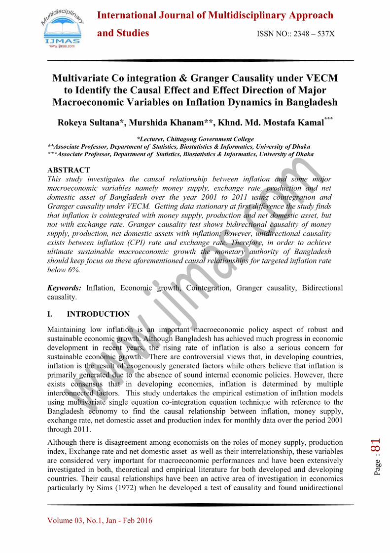
International Journal of Multidisciplinary Approach

and Studies ISSN NO:: 2348 – 537X

Volume 03, No.1, Jan - Feb 2016

Pag

e : 8

1

Multivariate Co integration & Granger Causality under VECM

to Identify the Causal Effect and Effect Direction of Major

Macroeconomic Variables on Inflation Dynamics in Bangladesh

Rokeya Sultana*, Murshida Khanam**, Khnd. Md. Mostafa Kamal***

*Lecturer, Chittagong Government College

**Associate Professor, Department of Statistics, Biostatistics & Informatics, University of Dhaka

***Associate Professor, Department of Statistics, Biostatistics & Informatics, University of Dhaka

ABSTRACT

This study investigates the causal relationship between inflation and some major

macroeconomic variables namely money supply, exchange rate, production and net

domestic asset of Bangladesh over the year 2001 to 2011 using cointegration and

Granger causality under VECM. Getting data stationary at first difference the study finds

that inflation is cointegrated with money supply, production and net domestic asset, but

not with exchange rate. Granger causality test shows bidirectional causality of money

supply, production, net domestic assets with inflation; however, unidirectional causality

exists between inflation (CPI) rate and exchange rate. Therefore, in order to achieve

ultimate sustainable macroeconomic growth the monetary authority of Bangladesh

should keep focus on these aforementioned causal relationships for targeted inflation rate

below 6%.

Keywords: Inflation, Economic growth, Cointegration, Granger causality, Bidirectional

causality.

I. INTRODUCTION

Maintaining low inflation is an important macroeconomic policy aspect of robust and

sustainable economic growth. Although Bangladesh has achieved much progress in economic

development in recent years, the rising rate of inflation is also a serious concern for

sustainable economic growth. There are controversial views that, in developing countries,

inflation is the result of exogenously generated factors while others believe that inflation is

primarily generated due to the absence of sound internal economic policies. However, there

exists consensus that in developing economies, inflation is determined by multiple

interconnected factors. This study undertakes the empirical estimation of inflation models

using multivariate single equation co-integration equation technique with reference to the

Bangladesh economy to find the causal relationship between inflation, money supply,

exchange rate, net domestic asset and production index for monthly data over the period 2001

through 2011.

Although there is disagreement among economists on the roles of money supply, production

index, Exchange rate and net domestic asset as well as their interrelationship, these variables

are considered very important for macroeconomic performances and have been extensively

investigated in both, theoretical and empirical literature for both developed and developing

countries. Their causal relationships have been an active area of investigation in economics

particularly by Sims (1972) when he developed a test of causality and found unidirectional




Pag

e : 8

2

causality from money to income for United States as claimed by the Monetarists. Afterwards,

Lee and Li (1983) found bidirectional causality between income and money and

unidirectional from money to prices for Singapore. Joshi and Joshi (1985) support their claim

from the evidence of Indian economy. However, Khan and Siddiqui (1990) found of

unidirectional causality from income to money and bidirectional between money and prices

in Pakistan. In the same line of research, Akash, et. al. (2011) claim that there exist long term

relationship among money supply, inflation and industrial production for Pakistan. Abbas

(1991) performed causality test between money and income for Asian countries and found

bidirectional causality in Pakistan, Malaysia and Thailand. Chimobi and Uche (2010) find

that money supply Granger causes both production and prices. However, Sharma, et.al.

(2010) indicate that output and prices do not Granger cause money supply reflecting

exogeneity of money supply. Therefore, for monetary policy stance it is imperative to

understand the temporal dimensions of income, money and price causal relationship.

Very recently, Kamal (2015) reveals a uniform directional causation between the supply of

money and price movements for Bangladesh. The Authors shows that causal and reverse

causal relations between money and product and money and prices vary across frequencies

while the causality running from money to output remains a short-run phenomenon. The

study also stipulates a unidirectional causality between money and prices, with causality

running from money supply to prices, which can be regarded as a piece of empirical evidence

supporting the monetarist claim. The study also demonstrates that short run causality from

money supply to output, long run causality from money supply to prices, as well as lack of

long run causality from money supply to output, all co-exist. This result is also supported by

Nucu (2011) in the case of Romanian economy.

Similarly, Das (2012) shows that there exists a bi-directional causality between per capita

electricity consumption and per capita GDP, per capita GDP and per capita income for

Bangladesh. Likewise, bi-directional causality between budget deficit and nominal effective

exchange rates exist for Indian economy, although the relationships between budget deficit

and GDP, Money supply & CPI are not significant for Indian economy (Srivyal and Venkata,

2004). Comparable result follows for Greece (Andreas and Anastasios ,2011). Akinbobola

(2012) finds a causal linkage between inflation, money supply and exchange rate in Nigeria.

Nwosa and Oseni (2012) support this claim. Asari, et. al. (2011) show that interest rate

moves positively while inflation rate goes negatively towards exchange rate volatility in

Malaysia. Gokal and Hanif (2004) have revealed that the causality between the two variables

ran one-way from GDP growth to inflation.

In spite of immense body of literature, there has been miniature evidence for causal

relationship between these important macroeconomic variables together, especially no

evidence in the context of Bangladesh. This paper seeks to redress this gap by examining the

causal effect and direction of causality between the variables inflation, money supply,

exchange rate, production & net domestic asset in Bangladesh on monthly data under Vector

Error Correction Mechanism (VECM).

II. DATA AND VARIABLES

In this study, the monthly data of five time series variables- Consumer price index general (as

proxy of Inflation) using the base as 1995-96, Broad money M2 (as proxy of money supply)




Pag

e : 8

3

in 10 millions BDT, Quantum index for industrial production (all industries) using the base as

1988-89, Net domestic asset in 10 millions (crore) BDT & Exchange rate (BDT per US

dollar) from July 2001 to September 2011 that is 122 sample points have been used. The

variable have been named as cpigen, monsup2, qiip, ntdmast & usdollar respectively. The

data have been collected from ‗Monthly statistical bulletin’ of Bangladesh published by

Bangladesh Bureau of Statistics.

III. METHODOLOGY

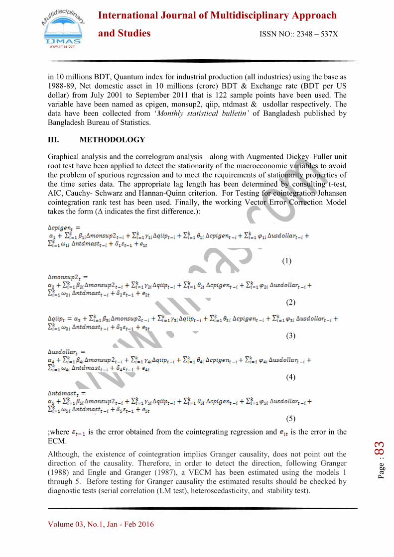
Graphical analysis and the correlogram analysis along with Augmented Dickey–Fuller unit

root test have been applied to detect the stationarity of the macroeconomic variables to avoid

the problem of spurious regression and to meet the requirements of stationarity properties of

the time series data. The appropriate lag length has been determined by consulting t-test,

AIC, Cauchy- Schwarz and Hannan-Quinn criterion. For Testing for cointegration Johansen

cointegration rank test has been used. Finally, the working Vector Error Correction Model

takes the form (∆ indicates the first difference.):

(1)

(2)

(3)

(4)

(5)

;where is the error obtained from the cointegrating regression and is the error in the

ECM.

Although, the existence of cointegration implies Granger causality, does not point out the

direction of the causality. Therefore, in order to detect the direction, following Granger

(1988) and Engle and Granger (1987), a VECM has been estimated using the models 1

through 5. Before testing for Granger causality the estimated results should be checked by

diagnostic tests (serial correlation (LM test), heteroscedasticity, and stability test).




Pag

e : 8

4

IV. RESULTS AND DISCUSSIONS

Descriptive statistics presented in table 1 shows that primarily the data is valid enough to

employ the specified techniques for analysis.

Table1: Descriptive Statistics of the five macroeconomic variables.

Variable Mean Standard

deviation Minimum Maximum Observation

Consumer price index

general 177.937 37.3688 128.44 259.66 122

Broad money M2 208582.4 102236 87452.7 453578.6 122

Quantum index for

industrial production 350.6901 90.39852 216.57 567.6 122

TK per us dollar 65.15287 5.369524 57 74.48 122

Net Domestic Asset 178300.1 82109.5 80135 381023.9 122

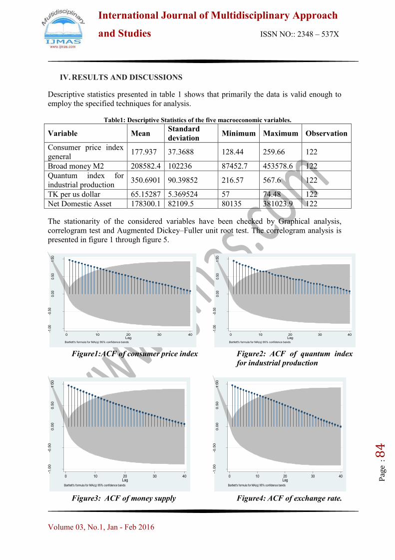
The stationarity of the considered variables have been checked by Graphical analysis,

correlogram test and Augmented Dickey–Fuller unit root test. The correlogram analysis is

presented in figure 1 through figure 5.

-1.0

0-0

.50

0.0

00.5

01.0

0

Auto

corr

ela

tions

of

cpig

en

0 10 20 30 40Lag

Bartlett's formula for MA(q) 95% confidence bands

Figure1:ACF of consumer price index

-1.0

0-0

.50

0.0

00.5

01.0

0

Auto

corr

ela

tions

of

qiip

0 10 20 30 40Lag


Figure2: ACF of quantum index

for industrial production

-1.0

0-0

.50

0.0

00.5

01.0

0

Auto

corr

ela

tions o

f m

onsup2

0 10 20 30 40Lag


Figure3: ACF of money supply

-1.0

0-0

.50

0.0

00.5

01.0

0

Auto

corr

ela

tions o

f usdoller

0 10 20 30 40Lag


Figure4: ACF of exchange rate.




Pag

e : 8

5

-1.0

0-0

.50

0.00

0.50

1.00

Aut

ocor

rela

tions

of n

tdm

ast

0 10 20 30 40Lag


Figure5: ACF of net domestic asset.

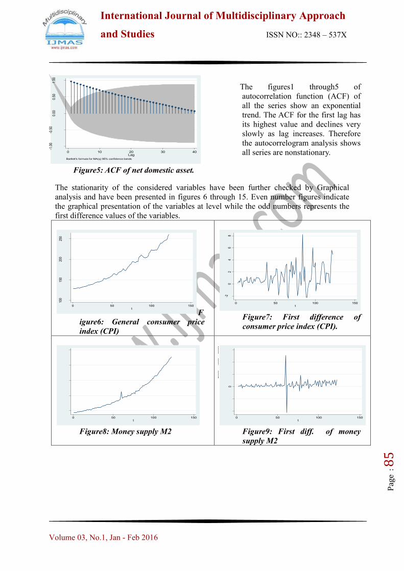
The figures1 through5 of

autocorrelation function (ACF) of

all the series show an exponential

trend. The ACF for the first lag has

its highest value and declines very

slowly as lag increases. Therefore

the autocorrelogram analysis shows

all series are nonstationary.

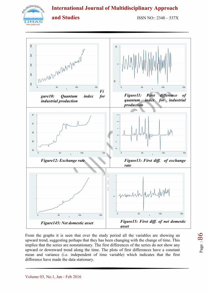
The stationarity of the considered variables have been further checked by Graphical

analysis and have been presented in figures 6 through 15. Even number figures indicate

the graphical presentation of the variables at level while the odd numbers represents the

first difference values of the variables.

100

150

200

250

cpig

en

0 50 100 150t

F

igure6: General consumer price

index (CPI)

-20

24

68

D.c

pige

n

0 50 100 150t

Figure7: First difference of

consumer price index (CPI).

1000

0020

0000

3000

0040

0000

5000

00m

onsu

p2

0 50 100 150t

Figure8: Money supply M2

-400

00-2

0000

0

2000

040

000

6000

0

D.m

onsu

p2

0 50 100 150t

Figure9: First diff. of money

supply M2




Pag

e : 8

6

200

300

400

500

600

qiip

0 50 100 150t

Fi

gure10: Quantum index for

industrial production

-50

050

D.q

iip

0 50 100 150t

Figure11: First difference of

quantum index for industrial

production

5560

6570

75

usdo

ller

0 50 100 150t

Figure12: Exchange rate

-2-1

01

23

D.u

sdol

ler

0 50 100 150t

Figure13: First diff. of exchange

rate

100000

200000

300000

400000

ntd

mast

0 50 100 150t

Figure145: Net domestic asset

-200

00-1

0000

0

1000

020

000

3000

0

D.n

tdm

ast

0 50 100 150t

Figure15: First diff. of net domestic

asset

From the graphs it is seen that over the study period all the variables are showing an

upward trend, suggesting perhaps that they has been changing with the change of time. This

implies that the series are nonstationary. The first differences of the series do not show any

upward or downward trend along the time. The plots of first differences have a constant

mean and variance (i.e. independent of time variable) which indicates that the first

difference have made the data stationary.




Pag

e : 8

7

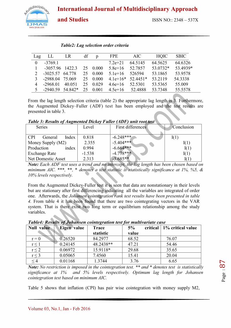
Table2: Lag selection order criteria

Lag LL LR df p FPE AIC HQIC SBIC

0 -3769.1 7.2e+21 64.5145 64.5625 64.6326

1 -3057.96 1422.3 25 0.000 5.8e+16 52.7857 53.0732* 53.4939*

2 -3025.57 64.778 25 0.000 5.1e+16 526594 53.1865 53.9578

3 -2988.04 75.069 25 0.000 4.1e+16* 52.4451* 53.2119 54.3338

4 -2968.01 40.051 25 0.029 4.6e+16 52.5301 53.5365 55.009

5 -2940.59 54.842* 25 0.001 4.5e+16 52.4888 53.7348 55.5578

From the lag length selection criteria (table 2) the appropriate lag length is 3. Furthermore,

the Augmented Dickey–Fuller (ADF) test has been employed and the test results are

presented in table 3.

Table 3: Results of Augmented Dickey Fuller (ADF) unit root test

Series Level First differences Conclusion

CPI General Index

Money Supply (M2)

Production index

Exchange Rate

Net Domestic Asset

0.818

2.355

0.994

-1.538

2.313

-6.248***

-5.404***

-6.664***

-4.778***

-3.685**

I(1)

I(1)

I(1)

I(1)

I(1)

Note: Each ADF test uses a trend and no intercept, the lag length has been chosen based on

minimum AIC. ***, **, * denotes a test statistic is statistically significance at 1%, %5, &

10% levels respectively.

From the Augmented Dickey-Fuller test it is seen that data are nonstationary in their levels

but are stationary after first differencing indicating all the variables are integrated of order

one. Afterwards, the Johansen cointegration rank test results have been presented in table

4. From table 4 it has been found that there are two cointegrating vectors in the VAR

system. That is there exist two long term or equilibrium relationship among the study

variables.

Table4: Results of Johansen cointegration test for multivariate case

Null value Eigen value Trace

statistic

5% critical

value

1% critical value

r = 0 0.26520 84.2977 68.52 76.07

r ≤ 1 0.24145 48.2438** 47.21 54.46

r ≤ 2 0.06972 15.9118* 29.68 35.65

r ≤ 3 0.05065 7.4560 15.41 20.04

≤ 4 0.01168 1.3744 3.76 6.65

Note: No restriction is imposed in the cointegration test. ** and * denotes test is statistically

significance at 1% and 5% levels respectively. Optimum lag length for Johansen

cointegration test based on minimum AIC.

Table 5 shows that inflation (CPI) has pair wise cointegration with money supply M2,




Pag

e : 8

8

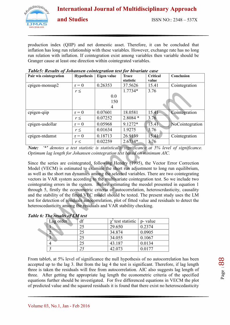
production index (QIIP) and net domestic asset. Therefore, it can be concluded that

inflation has long run relationship with these variables. However, exchange rate has no long

run relation with inflation. If cointegration exist among variables then variable should be

Granger cause at least one direction within cointegrated variables.

Table5: Results of Johansen cointegration test for bivariate case Pair wis cointegration Hypothesis Eigen value Trace

statistic

Critical

value

Conclusion

cpigen-monsup2 r = 0 0.26353 37.5626 15.41 Cointegration

1r

0.0

150

4

1.7734* 3.76

cpigen-qiip r = 0 0.07601 18.0581 15.41 Cointegration

1r 0.07252 2.8084 * 3.76

cpigen-usdollar r = 0 0.05968 9.1272* 15.41 NoCointegration

1r 0.01634 1.9275 3.76

cpigen-ntdamst r = 0 0.18713 26.9139 15.41 Cointegration

1r 0.02259 2.6734* 3.76

Note: ‘*’ denotes a test statistic is statistically significance at 5% level of significance.

Optimum lag length for Johansen cointegration test based on minimum AIC.

Since the series are cointegrated, following Hendry (1995), the Vector Error Correction

Model (VECM) is estimated to examine the short run adjustment to long run equilibrium,

as well as the short run dynamics among the selected variables. There are two cointegrating

vectors in VAR system according to the multivariate cointegration test. So we include two

cointegrating errors in the system. Before estimating the meodel presented in equation 1

through 5, firstly the econometric criteria of autocorrelation, heteroscrdasticity, causality

and the stability of the fitted VEC model should be tested. The present study uses the LM

test for detection of residuals autocorrelation, plot of fitted value and residuals to detect the

heteroscedasticity among the residuals and VAR stability checking.

Table 6: The results of LM test

Lag order df χ2

test statistic p- value

1 25 29.650 0.2374

2 25 34.874 0.0905

3 25 34.055 0.1067

4 25 43.187 0.0134

5 25 42.073 0.0177

From table6, at 5% level of significance the null hypothesis of no autocorrelation has been

accepted up to the lag 3. But from the lag 4 the test is significant. Therefore, if lag length

three is taken the residuals will free from autocorrelation. AIC also suggests lag length of

three. After getting the appropriate lag length the econometric criteria of the specified

equations further should be investigated. For five differenced equations in VECM the plot

of predicted value and the squared residuals it is found that there exist no heteroscedasticity




Pag

e : 8

9

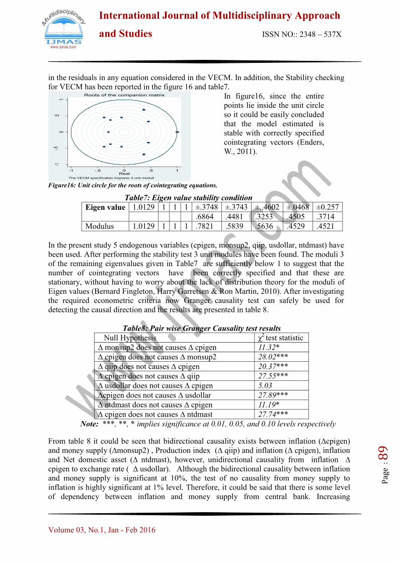
in the residuals in any equation considered in the VECM. In addition, the Stability checking

for VECM has been reported in the figure 16 and table7.

-1-.5

0.5

1

Imag

inary

-1 -.5 0 .5 1Real

The VECM specification imposes 3 unit moduli

Roots of the companion matrix

In figure16, since the entire

points lie inside the unit circle

so it could be easily concluded

that the model estimated is

stable with correctly specified

cointegrating vectors (Enders,

W., 2011).

Figure16: Unit circle for the roots of cointegrating equations.

Table7: Eigen value stability condition

Eigen value 1.0129 1 1 1 ±.3748 ±.3743 ±..4602 ±.0468 ±0.257

.6864 .4481 .3253 .4505 .3714

Modulus 1.0129 1 1 1 .7821 .5839 .5636 .4529 .4521

In the present study 5 endogenous variables (cpigen, monsup2, qiip, usdollar, ntdmast) have

been used. After performing the stability test 3 unit modules have been found. The moduli 3

of the remaining eigenvalues given in Table7 are sufficiently below 1 to suggest that the

number of cointegrating vectors have been correctly specified and that these are

stationary, without having to worry about the lack of distribution theory for the moduli of

Eigen values (Bernard Fingleton, Harry Garretsen & Ron Martin, 2010). After investigating

the required econometric criteria now Granger causality test can safely be used for

detecting the causal direction and the results are presented in table 8.

Table8: Pair wise Granger Causality test results

Null Hypothesis χ2

test statistic

∆ monsup2 does not causes ∆ cpigen 11.32*

∆ cpigen does not causes ∆ monsup2 28.02***

∆ qiip does not causes ∆ cpigen 20.37***

∆ cpigen does not causes ∆ qiip 27.55***

∆ usdollar does not causes ∆ cpigen 5.03

∆cpigen does not causes ∆ usdollar 27.89***

∆ ntdmast does not causes ∆ cpigen 11.19*

∆ cpigen does not causes ∆ ntdmast 27.74***

Note: ***, **, * implies significance at 0.01, 0.05, and 0.10 levels respectively

From table 8 it could be seen that bidirectional causality exists between inflation (∆cpigen)

and money supply (∆monsup2) , Production index (∆ qiip) and inflation (∆ cpigen), inflation

and Net domestic asset (∆ ntdmast), however, unidirectional causality from inflation ∆

cpigen to exchange rate ( ∆ usdollar). Although the bidirectional causality between inflation

and money supply is significant at 10%, the test of no causality from money supply to

inflation is highly significant at 1% level. Therefore, it could be said that there is some level

of dependency between inflation and money supply from central bank. Increasing




Pag

e : 9

0

government borrowing from central bank is seen as highly inflationary in the case of

Bangladesh. However, there is a general consensus among economists and policy-makers that

regulating the growth of money stock is necessary to achieve a fairly stable price level and

full employment of an economy (Sims 1972).

From the bidirectional causality among production and inflation it could be said that

production and inflation is strongly related to each other. Accordingly if the production level

of a country could be made stable then inflation could be also made stable. Net domestic

asset in Bangladesh is the aggregate of net foreign asset, domestic credit government (net)

and domestic credit public sector (BBS). Increase in lending means the bank will get

increased return from the borrowers by adding the interest rate with the return. And increase

in borrowing for a bank means the bank will have to pay interest on the return. If there is no

balance between these two factors then it results high inflation. As a result, balance between

lending and borrowing should be maintained to get a stable inflation.

V. CONCLUSION

This study investigates the causal relationship of money supply, exchange rate, production

index and net domestic asset to inflation rate in Bangladesh over the time period July 2001

to September 2011 in monthly basis. Results show that the data are nonstationary at their

level but stationary at their first difference. Lagged value has been selected as suggested by

AIC. Johansen cointegration rank test shows that there are two cointegrating equations i.e.

long term causal relationship exists. Based on Johansen cointegration rank test Vector Error

Correction Model (VECM) has been applied to find out the short term dynamics of

causality. Granger Causality under VECM is used to find the direction of causality. The

study is concerned with the causality from the specified macroeconomic variables to the

inflation rate in Bangladesh. The pair wise Granger causality test has reflected the

bidirectional causality between inflation (CPI) and money supply (M2), Production index

and inflation, inflation and Net domestic asset, while, unidirectional causality from inflation

to exchange rate. The study results show that money supply is related to inflation; hence,

the authority has to control the excess supply of money. And for that the government has to

maintain a consistent balance between consumption and expenditure so that the adjustment

in the budget deficit could not increase the level of money supply. Moreover, to strengthen

local currency Government has to increase Domestic Production, above all, local

production must be encouraged to boost domestic production and income and reduce

leakages of foreign exchange. Furthermore, a balance between lending and borrowing

should be maintained to get a stable inflation.

REFERENCES

i. Abbas, K. (1991). Causality Test between Money and Income: A Case Study of

Selected Developing Asian Countries (1960—1988). The Pakistan Development

Review, Vol. 30(4): 919–929.

ii. Akash, R.S.I. et al. (2011), ―Co integration and causality analysis of dynamic linkage

between economic forces and equity market: An empirical study of stock returns

(KSE) and macroeconomic variables (money supply, inflation, interest rate, exchange




Pag

e : 9

1

rate, industrial production and reserves)‖, African Journal of Business Management,

vol. 5(27), 10940-10964.

iii. Akinbobola, T.O.(2012), ―The dynamics of money supply, exchange rate and

inflation in Nigeria‖, Journal of Applied Finance & Banking, 2(4),117-141.

iv. Andreas, G.G. (2011), ―The macroeconomic effects of budget deficits in Greece: A

VAR-VECM approach‖, International Research Journal of Finance and Economics,

Issue.79.

v. Asari, F.F.A.H. et al. (2011), ―A vector error correction model (VECM) approach in

explaining the relationship between interest rate and inflation towards exchange rate

volatility in Malaysia‖, World Applied Sciences Journal, 12, 49-56.

vi. Bangladesh Bureau of Statistics (BBS), (2001- 2011). Statistical Pocket Book of

Bangladesh 2012. Dhaka: Bangladesh Bureau of Statistics (BBS), Ministry of

Planning, Government of the People‘s Republic of Bangladesh.

vii. Bangladesh Economic Update (2011), Food prices and inflation trajectory,

Bangladesh Economic Update, 2(1)

viii. Bernard Fingleton, Harry Garretsen & Ron Martin (2010), ―Recessionary Shocks and

Regional Employment: Evidence on the Resilience of UK Regions‖, Department of

Economics, University of Strathclyde, UK.

ix. Chimobi, O. P., & Uche, U. C. (2010). Money, Price and Output: A Causality Test for

Nigeria. American Journal of Scientific Research, 8, 78-87.

x. Das, J. (2012), ―Causality relationship among electricity consumption, energy use,

income, expenditure and GDP in Bangladesh: A Vector Error Correction Model

approach‖, Unpublished MS Thesis, Session: 2009-2010, Department of Statistics,

Biostatistics & Informatics, University of Dhaka.

xi. Enders, W. (2011), Applied Econometric Time Series, 2nd Edition, John Wiley and

Sons, Inc.

xii. Engel, R.F. and Granger, C.W.J. (1987), ―Cointegration and error correction:

representation, estimation and testing‖, Econometrica, 55, 251-276.

xiii. Granger, C.W.J.(1988), ―Causality, cointegration and control‖ , Journal of Economic

Dynamics and control, 12, 551-559.

xiv. Gokal, V. and Hanif, S.(2004). ―Relationship between inflation and economic

geowth‖, Economics Department, Reserve Bank of Fiji, Working Paper-2004/04.

xv. Hendry, S. (1995). ―Long-Run Demand for M1.‖ Bank of Canada Working Paper No.

95–11.

xvi. Johansen, S. (1988). ―Statistical analysis of cointegrating vectors‖ , Journal of

Economic Dynamics and control, 12, 231-254.

xvii. Kamal, K. M. (2014). Investigating Long-run Relationship between Money,

Income and Price for Bangladesh: Application of Econometrics and Cross Spectra

Methods, Journal of Science Foundation, 12(2).




Pag

e : 9

2

xviii. Khan, A., and Siddiqui A. (1990). Money, Prices and Economic Activity in Pakistan:

A Test of Causal Relation. Pakistan Economic and Social Review, winter, 121–136.

xix. Lee, S., and Li W. (1983), Money, Income, and Prices and their Lead-lag Relationship

in Singapore. Singapore Economic Review, April, 73–87.

xx. Matin, A. (2011). ―Inflation in Bangladesh: Driven by global phenomena‖,

Bangladesh: BRAC Stock Brokerage Limited.

xxi. Nucu, A.E. (2011). ―The relationship between exchange rate and key macroeconomic

indicators. Case study: Romania‖, The Romanian Economic Journal, XIV,l-41.

xxii. Nowsa, P. I. and Oseni, I. O. (2012). ―Monetary policy, exchange rate and inflation

rate in Nigeria: A co-integration and multivariate vector error correction model

approach‖, Research Journal of Finance and Accounting, 3(3).

xxiii. Sharma A, Kumar A, Hatekar N (2010). ―Causality between Prices, Output and

Money in India: An Empirical Investigation in the Frequency Domain‖, Centre for

Computational Social Sciences, University of Mumbai , Discussion Paper No.3, 1-18.

xxiv. Sims, C. (1972). ―Money, income and causality‖, The American Economic Review,

62(3), 540-52.

xxv. Srivyal, V. and Venkata, S.S.(2004). ―Budget deficits and other macroeconomic

variables in India‖, Applied Econometrics and International Development, 4(1).

xxvi. Tabas, H. M. et. al.(2012). ―The effect of the real effective exchange rate fluctuations

on macroeconomic indicators (Gross Domestic Product (GDP), Inflation and Money

Supply)‖, Interdisciplinary Journal of Contemporary Research in Business, 4 (6).

Documents

Multivariate Co integration & Granger Causality under VECM ... · PDF fileMacroeconomic Variables on Inflation Dynamics in Bangladesh ... Granger causality under VECM. Getting data