Multivariate Analysis of Manufacturing Data

by

Ronald Cao

Submitted to the Department of Electrical Engineering and ComputerScience

in partial fulfillment of the requirements for the degree of

Master of Engineering and Bachelor of Science in Electrical Engineering

at the

MASSACHUSETTS INSTITUTE OF TECHNOLOGY

June 1997

@ Massachusetts Institute of Technology 1997. All rights reserved.

The author hereby grants to MIT permission to reproduce and distributepublicly paper and electronic copies of this thesis document in whole or in

part, and to grant others the right to do so.

Author .............. .. . ........ "" ......... ..... ..nDepartment of Electrical " ineering and Computer Science

May 23, 1997

Certified by ................. ~... .. -,. . ......David

Professor of Electrical EngineeringS- Thesis Supervisor

1\

Accepted by................. ... ... .........."rederig- R. Morgenthaler

:C ,Department Con~itee onorn ate Students

/

Multivariate Analysis of Manufacturing Databy

Ronald Cao

Submitted to the Department of Electrical Engineering and Computer Scienceon May 23, 1997, in partial fulfillment of the

requirements for the degree ofMaster of Engineering and Bachelor of Science in Electrical Engineering

Abstract

With the advancement of technology, manufacturing systems have become increasingly com-plex. Currently, many continous-time manufacturing-processes are operated by a compli-cated array of computers which monitor thousands of control variables. It has become moredifficult for managers and operators to determine sources of parameter variation and tocontrol and maintain the efficiency of their manufacturing processes.

The goal of this thesis is to present a sequence of multivariate analysis techniques that canbe applied to the analysis of information-rich data sets from web manufacturing processes.The focus is on three main areas: identifying outliers, determining relationships among vari-ables, and grouping variables. The questions asked are 1) how to effectively separate outliersfrom the main population? 2) how to determine correlations among variables or subpro-cesses? and 3) what are the best methods to categorize and group physically significantvariables within a multivariate manufacturing data set?

Results of various experiments focused on the above three areas include 1) both nor-malized Euclidean distance and principal component analysis are effective in separating theoutliers from the main population, 2) correlation analysis of Poisson-distributed defect den-sities shows the difficulties in determining the true correlation between varibles, and 3) bothprincipal component analysis with robust correlation matrix and principal component anal-ysis with frequency-filtered variables are effective in grouping variables. Hopefully theseresults can lead to more comprehensive research in the general area of data analysis ofmanufacturing processes in the future.

Thesis Supervisor: David H. StaelinTitle: Professor of Electrical Engineering

Acknowledgments

It has been an incredibly meaningful and fulfilling five years at MIT. The following are justsome of names of the people who have made tremendous contributions to my intellectualdevelopment and my personal growth.

* My advisor, Professor David Staelin, who provided me with the guidance that I neededon my research and thesis. He has inspired me with insightful ideas and thought-provoking concepts. In addition, he has given me the freedom to explore my ideas aswell as many valuable suggestions for experimentations.

* My lab partners: Junehee Lee, Michael Shwartz, Carlos Caberra, and Bill Blackwell.Many thanks to Felicia Brady.

* Dean Bonnie Walters, Professor George W. Pratt, Professor Kirk Kolenbrander, Pro-fessor Lester Thurow, and Deborah Ullrich.

* All the friends I have made through my college life, especially my good friends DavidSteel and Jake Seid and the brothers of Lambda Chi Alpha Fraternity.

* Most of all, I would like to thank my parents for their endless love and support. Theyhave been there through every phase of my personal and professional development.Thank you!

Contents

1 Introduction 17

1.1 Background ................... . .. .. .. ..... ... .. 17

1.2 Previous W ork .................................. 18

1.3 O bjective . . . . . . . . . . . . . . . . . . . . . . . . . . . . . . . . ... . . 19

1.4 Thesis Organization ................................ 19

2 Basic Analysis Tools 21

2.1 Data Set ............. ...... .... .... ........ . . 21

2.2 Preprocessing .............. ..... .... .. ........ . . 22

2.2.1 M issing Data ............................... 22

2.2.2 Constant Variables ............................ 22

2.2.3 Norm alization ............................... 22

2.3 Outlier Analysis .................................. 24

2.3.1 Definition . .. ...... ... .. .. .. ... . ... .. . .. .. . 24

2.3.2 Causes of Outliers ............................ 24

2.3.3 Effects of Outliers .............................. .. 25

2.3.4 Outlier Detection ............................. 25

2.4 Correlation Analysis ............................... 26

2.5 Spectral Analysis ................................. 28

2.6 Principal Component Analysis ................... ....... 29

2.6.1 Basic Concept ............................... 29

2.6.2 Geometric Representation ................... ..... 29

2.6.3 Mathematical Definition ................... ...... 31

7

3 Web Process 1 35

3.1 Background .......................... ... ...... .. 35

3.2 Data ...................... ................ .. 35

3.3 Preprocessing .................... ................ 36

3.4 Feature Characterization ............................. 36

3.4.1 In-Line Data . .. ... .. .. .. .. ... .. .. .. .. .. . .. . 36

3.4.2 End-of-line Data ............... ............ .. 37

3.5 Correlation Analysis .................... ........... 39

3.5.1 Streak-Streak Correlation ........................ 39

3.5.2 Streak-Cloud Correlation ......................... 41

3.5.3 Interpretation .................... ....... ..... 42

3.6 Poisson Distribution ............................... 43

3.6.1 M ethod . . . . . . . . . . . . . . . . . . . . . . . . . . . . . . . .. . 43

3.6.2 Results............. ................... ..... 44

3.7 Principal Component Analysis ............ .. ....... ..... . 45

3.7.1 PCA of the End-of-Line Data ...................... 45

3.7.2 PCA of the In-Line Data ......................... 45

3.7.3 Interpretation .................. ........... .. 47

4 Web Process 2 49

4.1 Background ........ .... ....... ....... ......... . 49

4.2 D ata . . . . . .... . . . . . . . . . . . . . . . . . . . . . . . . . . . . . . . . 50

4.3 Preprocessing .......... .. . ............. .......... 50

4.4 Feature Characterization ................. ............ 50

4.4.1 Quality Variables ........ ........... ... .. .... .. 50

4.4.2 In-Line Variables ...................... ....... .. ...... 51

4.5 Outliers Analysis ................................. ............ 52

4.5.1 Normalized Euclidean Distance ... . . . ................ 52

4.5.2 Time Series Model - PCA .. ..... .............. .... 53

4.5.3 Identifying Outlying Variables ............. . . . . . . . . . . 58

4.6 Variable Grouping ... ... ............................ 62

4.6.1 Principal Component Analysis ....................... . . . . . 62

4.6.2 PCA with Robust Correlation Matrix . ................. 64

4.6.3 PCA with Frequency-Filtered Variables. ... . .. ....... 72

5 Conclusion and Suggested Work 79

List of Figures

2-1 (a) Plot in Original Axes (b) Plot in Transformed Axes . ........... 30

3-1 Time-Series Behavior of a Typical In-Line Variable . . . . . . . . . . . . . . 37

3-2 Cross-Web Position of Defects Over Time . .................. . 37

3-3 Streak and Cloud Defects ............................ 38

3-4 The 10 Densest Streaks Over Time ....................... 40

3-5 Correlation Coefficients Between Streaks Using a) standard time block, b)

double-length time block, c) quadruple-length time block . .......... 41

3-6 Correlation Coefficients Between Streak and Cloud with Time Blocks of length

1 to length 100 . . .. .. . .. .. .. .. . . . .. .. . . .. . . . . . .. . 42

3-7 (a) Cloud Distribution Using Fixed-Length Time Blocks, (b) Ideal Poisson

Distribution Using the Same Fixed-Length Time Blocks . ........... 43

3-8 Distributions of Cloud Defects Using x2, x4, and x6 Time Blocks ....... 44

3-9 Ideal Poisson Distributions Using x2, x4, and x6 Time Blocks . ....... 44

3-10 First 3 Principal Components of the End-of-Line Data . ........... 46

3-11 Percent of Variance Captured by PCs ...................... 46

3-12 First 4 PCs of the In-Line Data ......................... 47

4-1 Ten Types of In-Line Variable Behavior ................... .. 51

4-2 Normalized Euclidean Distance ................... ...... 53

4-3 Outlier and Normal Behavior Based on Normalized Euclidean Distance . . . 54

4-4 First Ten Principal Components of Web Process 2 Data Set . ........ 55

4-5 High-Pass Filters with Wp=0.1 and Wp = 0.3 . ................ 56

4-6 First Ten Principal Components from 90% High-Pass Filterd Data ...... 57

4-7 First Ten Principal Components from 70% High-Pass Filtered Data .... . 57

4-8 Variables Identified that Contribute to Transient Outliers in Region 1 and 4 60

4-9 The First Principal Component and the Corresponding Eigenvector from Pro-

cess 2 Data ....... .............. .............. . 60

4-10 The First Ten Principal Components from 738 Variables . .......... 61

4-11 The First Ten Eigenvectors from 738 Variables . ................ 61

4-12 First 10 Eigenvectors of 738 Variables ........ . .............. . 63

4-13 Histograms of the First 10 Eigenvectors of 738 Variables . .......... 63

4-14 Magnitude of Correlation Coefficients of 738 Variables in Descending Order

in (a) Normal Scale, (b) Log Scale ........................ 65

4-15 1st 10 Eigenvectors of Calculated from Robust Correlation Matrix with Cutoff

= 0.06 . . . . . . . . . . . . . . . . . . . . . . . . . . . . . . . . . . . . . . . 66

4-16 Histograms of the first 10 Eigenvectors Calculated from Robust Correlation

M atrix with Cutoff = 0.06 ......... .................... 66

4-17 1st 10 Eigenvectors of Calculated from Robust Correlation Matrix with Cutoff

= 0.1 . . . . . . . . . . . . . . . . . . . . . . . . . . . . . . . . . . .. . . 67

4-18 Histograms of the first 10 Eigenvectors Calculated from Robust Correlation

M atrix with Cutoff = 0.10 ............................ 67

4-19 First 10 Eigenvectors calculated from Correlation Matrix with Cutoff at 0.15 68

4-20 Histogram of First 10 Eigenvectors calculated from Robust Correlation Matrix

with Cutoff at 0.15 ....... ................. ........ 68

4-21 First 10 Eigenvectors calculated from Robust Correlation Matrix with Cutoff

at 0.18 ... ..................... .... .. ......... .. 69

4-22 Histogram of First 10 Eigenvectors calculated from Robust Correlation Matrix

with Cutoff at 0.18 ........ ...................... ... 69

4-23 A Comparison of Eigenvectors Calculated from (a) Original Correlation Ma-

trix (b) Robust Correlation Matrix with Cutoff=0.06, (c) Robust Correlation

Matrix with Cutoff=0.10, (d) Robust Correlation Matrix with Cutoff=0.15,

(e) Robust Correlation Matrix with Cutoff=0.18 . ............... 71

4-24 A Comparison of Histograms of the Eigenvectors . .............. 71

4-25 (a) High-Pass Filter with Wp = 0.3 (b) Band-Pass Filter with Wp=[0.2, 0.4] 72

4-26 First 10 Eigenvectors Calculated from High-Pass Filtered (Wp=0.1) Variables 73

4-27 Histograms of First 10 Eigenvectors Calculated from High-Pass Filtered (Wp=0.1)

Variables . . . . . . . . . . . . . . . . . . . . . . . . . . . . . . . . . . . . . . 73

4-28 First 10 Eigenvectors Calculated from High-Pass Filtered (Wp=0.3) Variables 74

4-29 Histograms of First 10 Eigenvectors Calculated from High-Pass Filtered (Wp=0.3)

Variables . . . . . . . . . . . . . . . . . . . . . . . . . . . . . . . . . . . . . . 74

4-30 First 10 Eigenvectors Calculated from High-Pass Filtered (Wp=0.4) Variables 75

4-31 Histograms of First 10 Eigenvectors Calculated from High-Pass Filtered (Wp=0.4)

Variables . . . . . . . . . . . . . . . . . . . . . . . . . . . . . . . . . . . ... 75

4-32 First 10 Eigenvectors Calculated from Band-Pass Filtered (Wp=[0.2, 0.4])

V ariables . . . . . . . . . . . . . . . . . . . . . . . . . . . . . . . . . . . . . . 76

4-33 Histograms of First 10 Eigenvectors Calculated from Band-Pass Filtered (Wp=[0.2,

0.4]) Variables .................... ..... .. .. ...... 76

4-34 First 10 Eigenvectors Calculated from Band-Pass Filtered (Wp=[0.2, 0.3])

Variables . . . . . . . . . . . . . . . . . . . . . . . . . . . . . . . . . ... . . 77

4-35 Histograms of First 10 Eigenvectors Calculated from Band-Pass Filtered (Wp=[0.2,

0.3]) Variables . . . .. .. ... . . . . . . . . .. . . . . . . . . . . . . .. . 77

List of Tables

2.1 12 Observations of 2 Variables............. ..... ....... ..... 29

Chapter 1

Introduction

1.1 Background

With development of technology, manufacturing systems are getting increasingly more com-

plex. A typical continous-time manufacturing process may be controlled and monitored by

thousands parameters such as temperature and pressure. With higher customer standards

and higher operating cost, manufacturing companies are constantly creating new ways to

deal with the problem of how to increase efficiency and reduce cost.

The Leaders for Manufacturing (LFM) Program is a joint effort among leading U.S. man-

ufacturing firms and both the School of Engineering and the Sloan School of Management

from the Massachusetts Institute of Technology. The goal of LFM is to identify, discover,

and translate into practice the critical factors that underlie world-class manufacturing. MIT

faculty and students and participating LFM companies have identified seven major themes

of cooperation. These research themes are Product and Process Life Cycle, Scheduling

and Logistics Control, Variation Reduction, Design and Operation of Manufacturing Sys-

tems, Integrated Analysis and Development, Next Generation Manufacturing, and Culture,

Learning, and Organizational Change.

The research and analysis presented in this thesis is directly related to Leaders For

Manufacturing Research Group 4 (RG4) whose focus is variation reduction in manufacturing

processes. Understanding variations and methods to reduce them can help companies to

improve yields, reduce defects, decrease product cycle time, and generate higher quality

products. In order to gain this understanding, RG4 attempts to answer questions such

as 1) how to effectively determine which process parameters to monitor and control? 2)

what are useful technique to determine multivariate relationship among control and quality

variables? 3) How to best communicate results and findings to managers and engineers at

the participating companies?

There are many types of manufacturing processes in industry. The type of processes

that this thesis focuses on are referred to as web processes. The particular characteristic

associated with a web process is that the end product is in the form of sheets with the

appropriate thickness, width and length and can be packaged into rolls or sliced into sheets.

Although multivariate analysis methods are applied to two data sets collected from web

processes, most of the tools discussed in this thesis can also be applied to analyze data from

other types of processes.

1.2 Previous Work

My research builds on the work conducted by previous LFM RG4 research assistants. In his

Master's thesis titled "The treatment of Outliers and Missing Data in Multivariate Manu-

facturing Data", Timothy Derksen developed strategies for dealing with outliers and missing

data in largý, multivariate, manufacturing data.[2] He compared the effectiveness of statis-

tics based on standard versus robust estimates of the mean, standard deviation, and the

correlation matrix in separating the outliers from the main population. In addition, he

developed maximum likelihood methods to treat missing data in large multivariate manu-

facturing data. Mark Rawizza's "Time-Series Analysis of Multivariate Manufacturing Data

Sets" [4] discussed various data analysis tools used in engineering and applied them to manu-

facturing data sets. He used fundamental preprocessing and data-reduction techniques such

as principal component analysis to present and reorganize manufacturing data. Furthermore,

he experimented with ARMA models and neural networks to assess the predictability of data

sets collected from both web processes and wafer processes.

1.3 Objective

The objective of this thesis is to apply series of multivariate techniques to analyze information-

rich data sets from continous web manufacturing processes. In particular, a lot of the anal-

ysis is based on having an understanding of the physics behind the manufacturing process.

Combining multivariate analysis tools with an understanding of the underlying physics can

produce results and insights that can be very valuable company managers.

The questions asked in this thesis are: 1) how to effectively separate outliers from the

main population? 2) how to determine relationships among variables and subprocesses?

and 3) what are the best methods to categorize and group variables within an information-

rich multivariate data set? Results of various experiments focused on these three areas are

discussed. Hopefully they can lead to more comprehensive research in the general area of

data analysis of manufacturing processes in the future.

1.4 Thesis Organization

This thesis is divided into four major sections. Chapter 2 presents an overview of the major

multivariate analysis tools and methods used in the rest of the thesis. These tools deal with

preprocessing of the original data, outlier identification and analysis, correlation analysis,

spectral analysis, and principal component analysis.

Chapter 3, the second major section, utilizes the multivariate tools presented in Chapter

2 to analyze a web manufacturing data set. With the data set divided into in-line variables

and quality variables, the objective is to perform multivariate analysis on these two sets

of variables separately and to determine multivariate linear relationships between them. In

addition, correlation analysis is performed on Poisson-distributed defect densities.

Chapter 4, the third section, applies the basic tools to analyze a data set from a dif-

ferent manufacturing web process, where the in-line variables and the quality variables are

not identified. The analysis focuses on experimenting with ways to more effectively sep-

arate variables utilizing principal components. Experimental results show that PCA with

robust correlation coefficients and PCA with frequency-filtered variables are more effective

in grouping and identifying the variables that are correlated with each other.

Chapter 5, the final section, summarizes the important insights gained and suggests

possible areas of continued research.

Chapter 2

Basic Analysis Tools

2.1 Data Set

A data set contains information about a group of variables. The information is the values

of these variables for different times or situations. For cxample, we might have a data set

that consists of weather information for 50 states. There might be 20 variables such as

rainfall, average temperature, and dew point temperature, and 50 observations of these 20

variables representing the 50 states. The data set might also be the same 20 variables and

50 observations representing daily measurements of each of these 20 variables for one state

over 50 days. Both data sets can be represented as a m x n matrix, where m = 50 is the

total number of observations and n = 20 is the total number of variables.

The data sets used in this thesis are recorded from continous-time web manufacturing

systems. A typical data set may consists of measurements of thousand of variables for

thousands of observations recorded over days. The variables can be categorized as either in-

line variables or end-of-line variables. The in-line variables of a manufacturing system control

and monitor the operation of the manufacturing process. Some typical in-line variables are

temperature, pressure, volume, speed, and so on. Furthermore, end-of-line variables, also

referred to as quality variables, provide managers and technicians with information on the

quality of the end product of the manufacturing process. Some typical quality variables are

defect size, defect location, thickness and strength.

2.2 Preprocessing

Preprocessing the data is an integral part of data analysis. Very rarely can large new data

sets be used unaltered for multivariate analysis. The following are three major parts of

preprocessing:

2.2.1 Missing Data

Within a raw manufacturing data set, very rarely are all the observations complete, espe-

cially when measurements are collected over days. Often, parts of machines or subprocesses

are shut down for maintenance or testing purposes. As a result, certain parameters are not or

cannot be recorded. These missing observations need to be treated before any multivariate

analysis. Timothy Derksen, in "The treatment of Outliers and Missing Data in Multivariate

Manufacturing Data", investigated methods of detecting, characterizing, and treating miss-

ing data in large multivariate manufacturing data sets.[2] In general, if a variable has most

of its observations missing, the variable should be removed completely from the data set.

Otherwise, the missing observations can be estimated using the EM algorithm described by

Little.[6]

2.2.2 Constant Variables

Multivariate analysis allows for understanding variable behavior in a multi-dimensional

world. Any variables that are constant over time do not exhibit any information relevant to

multivariate analysis. As a result, variables that have zero variance should be removed from

the data set.

2.2.3 Normalization

For a web process data set that contains n variables and m observations, the n variables

can consist of both control and quality parameters such as temperature, pressure, speed,

thickness, density, and volume. Since all these variables are most likely measured in different

units, it is often very difficult to compare their relative values. To deal with this comparison

problem, normalization is applied to the variables.

For a given mxn matrix with i = 1, 2, . .. , m observations and j = 1, 2, . .. , n variables,

where the value of any ith observation and jth variable is denoted as Xej, the corresponding

value in the normalized data set is denoted as Zij.

Normalization is commonly defined as the following:

Zi = Xi - 9 (2.1)'Tj

where

Xj = '=1= xij (2.2)m

m - 1 (2.3)

In words, to calculate the normalized Zaj for any ith observation and jth variable, we take

the corresponding value Xij and subtract the mean Xj of the jth variable, and divide the

result by the standard deviation aj of the jth variable. In the rest of this thesis, a variable

that is said to be normalized is normalized to zero mean (Zi = 0) and unit variance (oa = 0).

There are benefits and drawbacks with performing normalization before multivariate

analysis. The following are reasons for normalization:

* Normalization causes the variables to be unit-less. For example, if the unit of Xij is

meters, Xij - Xj is also in meters. When the result is divided by aj, also measured

in meters, the final value Zii will be unit-less. As a result of normalization, variables

originally measured in different units can be compared with each other.

* Normalization causes all the variables to be weighted equally. Since the normalized

variables are zero-mean and unit-variance, each variable is weighted equally in de-

termining correlations among variables. Normalization is especially important before

performing multivariate analyses such as principal component analysis, because it gives

each variable equal importance. More on normalization and principal component anal-

ysis will be discussed in Section 2.6.

* Normalization is a way of protecting proprietary information inherent in the original

data. By taking away the mean and reshaping the variance, the information that is

proprietary can be removed. Protecting proprietary information is a very important

part of LFM's contract with its participating companies.

The following is one of the drawbacks of normalization:

* Normalization may increase the noise level. Since normalizing causes all the variables

to have unit variance, it is likely that some measured noise will be scaled so that it rivals

the more significant variables. As a result, normalization may distort the information

in the original data set by increasing the noise level.

2.3 Outlier Analysis

The detection and treatment of outliers are an important pre-step to performing statistical

analysis. This section defines outliers, names the causes and effects of outliers, and presents

some univariate and multivariate tools of detecting outliers.

2.3.1 Definition

Outliers are defined as a set of observations that are inconsistent with the rest of the data.

It is very important to understand that outliers are defined relative to the main population.

2.3.2 Causes of Outliers

The following are the causes of outliers:

1. Extreme members - Since manufacturing data consist of variables recorded over thou-

sands of observations, it is possible that some observations can occasionally exhibit

extreme values.

2. Contaminants - These are observations that should not be grouped with the main

population. For example, if the main population is a set of observations consisting the

weight of apples, the weight of an orange is considered a contaminant if it is placed

in the same group. In a manufacturing process, a contaminant can be an observation

made while a machine is broken amidst observations made while the machine is properly

operating.

2.3.3 Effects of Outliers

Statistical analysis without the removal of outliers can produce skewed and misleading re-

sults. Outliers can potentially drastically alter the sample mean and variance of a popu-

lation. In addition, outliers, especially contaminants, can incorrectly signal the occurrence

of extreme excursions in a manufacturing process when the process is actually operating

normally.

2.3.4 Outlier Detection

For a data set with n variables and m observations, a potential outlier is a point that

lies outside of the main cluster formed by the general population. The following are some

methods used to determine outliers.

Univariate Method An univariate method of detecting outliers is the calculated the

univariate number of standard deviations from the mean.

zij = (2.4)

where xij is the value of observation i and variable j, Tj is the sample mean of the variable

j, and aj is the sample standard deviation of the variable j. Observations where zij > Kj,

where Kj is a constant for variable j, can be categorized as outliers. Depending on the range

of the values of observations for each variable, the value of Kj can be adjusted. To determine

gross outliers, the value of Kj can be set to be large.

Multivariate Methods Equation 2.4 can be extended so that it represents a multivariate

measure of the distance of all the variables away from the origin. Observations where zj >

K, where K is a constant, can be treated as points lying outside of a n-dimensional cube

centered on the sample mean. This multivariate method is very similar to the univariate one,

except the value of K is constant for all variables. Similarly, this method can be effective in

determining gross outliers, but in a manufacturing environment where most of the variables

are correlated, this method is limited in its effectiveness in identifying outliers.

A more robust multivariate method to detect outliers involves calculating the Euclidean

distance to the origin of the n-dimensional space after all n variables are normalized to zero-

mean and unit-variance. The square of the normalized Euclidean distance is defined as the

following:N 2

d 2 = -- (2.5)j=1 si

where xij is the value of observation i for variable j, and sj is the sample variance of variable

j. Observations with d? > K, where K is a constant, lie outside of an ellipsoid centered

around the origin and are considered as outliers.

2.4 Correlation Analysis

In a multivariate manufacturing environment, it is often desirable to measure the linear

relationship between pairs of variables or among groups of variables. By understanding these

relationships among variables, managers can gain insights into the manufacturing process.

One method of determining the linear relationship between variables is to calculate their

covariance and correlation.

Given two variables i and j, with m observations, the sample covariance sij measures the

linear relationship between the two variables and is defined as the following:

sij = rs - a (ki -1i)(eke s e v) (2.6)k=l

For n variables, the sample covariance matrix S = (sij) is the matrix of sample variances

and covariances of combinations of the n variables:

S = (si) =

S11 312 ... Sin

821 S22 ... S2n

Sn1 Sn2 *.. Snn

where the diagonal of S represents the sample variances of the n variables, and rest of the

matrix represents all the possible sample covariances of pairs of Variables. The covariance of

the ith and jth variables, sij, is defined by Equation 2.6, and the variance, sij = s?, of the

same pair of variables is defined as the following:

i " m= - 1 (ki - -i) 2 (2.8)k=l

Since the covariance depends on the scale of measurement of variable i and j, it is difficult

to compare covariances between different pairs of variables. For example, if we change the

unit of a variable from meters to miles, that covariance will also change. To solve this

problem, we can normalize the covariance by dividing by the standard deviations of the two

variables. The normalized covariance is called a correlation.

The sample correlation matrix R can be obtained from the sample covariance matrix and

is defined as:

1 r12 ... rln

Rr21 1 ... r2n

rnl rn2 ... 1

(2.9)

where rij, the sample correlation coefficient of the ith and jth variable, is defined as the

following:

rn = (2.10)

Since the correlation of a variable with itself is equal to 1, the diagonal elements of matrix R

in Equation 2.9 are all is. In addition, please notice that if the variables are all normalized

to unit variance such that s;i =1 and sjj = 1, then the correlation matrix R is equal to the

(2.7)

covariance matrix S. Since most of the multivariate analysis discussed in this paper deals

with normalized variables, R is often substituted for S.

2.5 Spectral Analysis

Fourier Transform Fourier transforms can be an excellent tool to gain insight into the

behavior of variables in the frequency domain. For the jth variable observed at time i =

1, ..., m, the Fourier transform is defined as:

m

Xj(ew) = xiie - jwn (2.11)i=1

Autocorrelation Function The autocorrelation function looks at a variable's correlation

with itself over time. A typical random signal is more correlated with itself over short time

lag versus long time lag. The autocorrelation of variable xj is:

R j(r) = E [xizx(i-,,)] (2.12)

Power-Spectral Density Power-Spectral Density (PSD) is the Fourier transform of the

autocorrelation function of a random signal xj(t).

Payr(w) = F(Rxx,(r)) (2.13)

where F is the Fourier transform operator and Rxj, (7) is the autocorrelation of the random

signal xj(t). For simplicity, the ensemble average of xj(t) is assumed to be zero without

any loss of generality. The calculation of autocorrelation requires the ensemble average of

xj(t)xz(t - r). Since our data consist of one sample sequence for each variable, this ensemble

average is impossible to get. One technique to get around this problem is to assume the

sequence is ergodic. Then the PSD is the magnitude squared of the Fourier transform.

P=xj(w) = IF(xj(t))12 (2.14)

2.6 Principal Component Analysis

2.6.1 Basic Concept

Principal components analysis (PCA) is a mathematical method for expressing a data set in

an alternative way. The method involves using linear combinations of the original variable

to transform the data set onto a set of orthogonal axes. The main objective of principal

component analysis is two-fold: 1) data reduction, and 2) interpretation.

Principal components analysis is often referred to as data reduction rather than data

restatement, because it preserves the information contained in the original data in a quite

succinct way. Principal component analysis takes advantage of the relationship among the

variables to reduce the size of the data while maintaining most of the variance in the original

set. A data set with n variables and m observation can be reduced to a data set with k

principal components and m observations, where k < n. In addition, since PCA transforms

the original data into a new set of axes, it often reveal relationships that are buried in the

original data set. As a result, PCA is a powerful tool in multivariate analysis.

2.6.2 Geometric Representation

Principal components analysis can be best understood in terms of geometric representation.

We can start with a simple two-dimensional example. Table 2.1 shows 12 observations of 2

variables, X1 and X 2.

1 2 3 4 5 6 7 8 9 10 11 12

X1 8 4 5 3 1 2 0 -1 -3 -4 -5 -8X2 4 6 2 -2 3 -2 0 2 -2 -6 -1 -3

Table 2.1: 12 Observations of 2 Variables

Figure 2-1 represents the data in Table 2-1 using two different sets of axes. The points

in Figure 2-la are interpreted relative to the original set of axes, while the same points

-8 -6 -4 -2 0 2 4 6 8

(a) (b)

Figure 2-1: (a) Plot in Original Axes (b) Plot in Transformed Axes

are interpreted relative to a new set of orthogonal axes in Figure 2-lb. The information is

preserved as the axes are rotated.

Similar to Figure 2-1b, principal components are defined as a transformed set of coordi-

nate axes obtained from the original data used to describe the information content of the

data set. In a 2-dimensional data set. The first principal component is defined as the new

axis that captures most of the variability of the original data set. The second principal com-

ponent, perpendicular to the first one, is the axis that captures the second biggest variance.

The principal components are calculated in a minimal squared-distance sense. The distance

is defined as the perpendicular distance from the points to the candidate axis. The first

principal component is the axis where the sum of the squared-distance from the data points

to the axis is minimal among all possible candidates. The second principal component is

taken perpendicular to the first one, for which the sum of the squared distance is the second

smallest.

In a multivariate data set that extends over more 2 dimensions, PCA finds directions

in which multi-variable data contain big variances (therefore, much information). The first

principal component has the direction in which the data have the biggest variance. The

direction of the second principal component is that with the biggest variance among the

directions which are orthogonal to the direction of the first principal component, and so on.

After a few principal components, the remaining variance of the rest is typically small enough

I ' ' ' ' m · · · · I

I . . . . · I . . . . I

so that we can ignore them without losing much information. As a result, the original data

set with n dimensions (n variables) can be reduced to a new data set with k dimensions (k

principal components) where k < n.

2.6.3 Mathematical Definition

Principal component analysis takes advantage of the correlation among variables to find new

set of variables which reduce most of the variation within the data set to as few dimension

as possible. The following is the mathematical definition [3]:

Given a data set with n variables and m observations, the first principal components

must satisfy the following conditions:

1. z1 is linear function of the original variables.

zi = w11X 1 + W12X 2 + ... + wlnXn (2.15)

where w11, w12 , . . . , w• are constants defining the linear function.

2. Scaling of new variable z l .

w1 + 2 + ... + n =1 (2.16)

3. Of all the linear functions of the original variable that satisfy the above two conditions,

pick zl that has the maximum variance.

Consequently, the second principal component must satisfy the following conditions:

1. z 2 is linear function of the original variables.

Z2 = w 2 1X 1 + w 2 2X 2 +-...- + 2 n Xn (2.17)

where w21, w22, • • , w2n are constants defining the linear function.

2. Scaling of variable z 2.

2w + w2 + " + w2 = 1 (2.18)

3. zl and z 2 must be perpendicular.

Wllw21 + W12 22 + ...- + WlnW2n = 0 (2.19)

4. The values of z 2 must be uncorrelated with the values of zj.

5. Of all the linear functions of the original variable that satisfy the above three conditions,

pick z 2 that captures as possible of the remaining variance.

For a data set with n variables, there are a total of n possible principal components. Each

component is a linear combination of the original set of variables, is perpendicular to the

previously selected components, with values uncorrelated with the values from the previous

set of values, and which explains as much as possible of the remaining variance in the data.

In summary,

zl = W'1X = w11X1 + wl 2X 2 + ... + wi,X,

z2 = w'2X = w21XI + w22X 2 + ... + w2,Xn (2.20)

z, = w',X = w 1lX 1 + wn2X 2 + ... + WnX,

where random variable X' = [X1, X 2, X3 ,..., Xn] has a covariance matrix S with eigenvalue-

eigenvector pairs (A1, ex), (A2, e2), . • , (An, e,) where A1 > X 2 > ... > A, > 0. The

principal components are uncorrelated linear combinations zi, z2 , z3, . . . , zn, whose

variances, Var(zi) = wýSwi, are maximized.

It can be shown that principal components solely depend on the covariance matrix S of

X 1, X 2 , X 3 , . . ., Xn. This is an very important concept to understand. As described earlier,

the axes of the original data set can be rotated by multiplying each Xi by an orthogonal

matrix W:

zi = WXi (2.21)

Since W is orthogonal, W'W = I, and the distance to the origin X is unchanged:

z:zi = (WX,)'(WXi) = X W'WX, = X X, (2.22)

Thus an orthogonal matrix transformed Xi to a point zi that is the same distance from the

origin with the axes rotated.

Since the new variables zi, z2, z3, * . • , z, in z = WX are uncorrelated. Thus, the

sample covariance matrix of z must of the form:

Sz

s2z 1 0 ... 0

0 Sz 2 ... 0

0 0 ... s2,n

(2.23)

if z = WX, then S, = WSW', and thus:

s2 Z 0 ... 0

0 S2 z2 ... 0WSW' = (2.24)

0 0 ... S2zn

where S is the sample covariance matrix of X. In linear algebra, we know that given C'SC

= D, where C is an orthogonal matrix, S is a symmetric matrix, and D is a diagonal matrix,

the columns of the matrix C must be normalized eigenvectors of S. Since Equation 2.24

shows that orthogonal matrix W diagonalizes S, W must equal the transpose of the matrix

C whose columns are normalized eigenvectors of S. W can be written as the following:I

W

W'.

(2.25)

where w! is the ith normalized eigenvector of S. The principal components are trans-

formed variables zl = w'X, z2 = w'X,. . . , z = w'X in z = WX. For example, zl =

wllX 1 + W12X 2 + ... + WlnXn

In addition, the diagonal elements in Equation 2.24 are the eigenvalues of S. Thus the

W =

eigenvalues A1, A2 , . . . , An, of S are the variances of the principal components zi =W!X:

s2zi = Ai (2.26)

Since the eigenvalues of S are variances of the principal components, the percentage of the

total variance captured by the first k principal components can be represented as:

A1 + ..2 + Ak% of Variance Captured = (2.27)

2i=I Sii

The following is a summary of some interesting and useful properties of principal com-

ponents.(Johnson, Wichern, p. 342)

* Principal components are uncorrelated.

* Principal components have variances equal to the eigenvalues of the covariance matrix

S of the original data.

* The rows of the orthogonal matrix W correspond to the eigenvectors of S.

f)A

Chapter 3

Web Process 1

3.1 Background

The data set used in this chapter is collected from a continous web manufacturing process

where more than 850 in-line control parameters are constantly monitored. The end-of-

line data comes from an optical scanner sensitive to small light-scattering defects where 8

important quality parameters are measured with high precision. In this chapter, some of the

analysis tools described in Chapter 2 are ultilized to characterize the multivariate behavior

of the in-line data, the multi-variate behavior of the end-of-line data, and the statistical

relationship between the two.

3.2 Data

The data set from Web Process 1 consists of two major groups of variables: in-line variables

and end-of-line variables. The in-line data set consists of physical parameters that control

the production process, while the end-of-line data are parameters that indicate the quality

of the end product. The combined data set represents information for the manufacturing of

115 rolls of the end product.

The in-line data set contains 854 control parameters, measured approximately every 61

seconds for 4320 observations. The end-of-line data consist of 4836 measurements of 8 quality

parameters. The values of these quality parameters are collected by a real-time scanner that

sweeps across the web at constant frequency. One of the 8 quality variables is an indicator

of the type of defect that occurs at the end-of-line.

3.3 Preprocessing

As discussed in Chapter 2, raw data sets often need to be preprocessed before any multi-

variate analysis are performed. In the following two sections, techniques are applied to both

the in-line and end-of-line data in order to present more effectively the information in the

original data.

End-of-Line Data Sometimes the values of variables are not numeric. As a result, the

information contained in the variables must be encoded before any analysis. How to encode

these non-numeric values depends on the type of information they convey. For example, the

end-of-line data contains a variable that categorizes the different types of defects. There are

a total of 8 defect types, and each one of them is simply assigned a numeric value.

In-Line Data There are a total of 854 in-line parameters, measured approximately every

61 seconds for a period of 3 days. Of all these parameters, 194 variables are constant over

the entire period. These 194 variables can be discarded without any further investigation.

In addition, 222 variables are also eliminated, because they are simply averages of other

parameters. Consequently, 438 in-line parameters are left for analysis.

3.4 Feature Characterization

Before performing any multivariate analysis, much insight can be obtained from examining

the data in the time and space domain.

3.4.1 In-Line Data

The in-line variables show fluctuations over time. This means the physical process does not

remain steady. It tends to change "significantly" over time. The following is a plot of the

behavior of a typical in-line parameter over time.

Figure 3-1: Time-Series Behavior of a Typical In-Line Variable

3.4.2 End-of-line Data

The end-of-line data, include the sizes, shapes, positions and times of defects. Figure 3-2 is a

visual representation of the positions and times of the defects. The horizontal axis represents

the cross-web position, and the vertical axis represents the times when defects occur. Each

point on the graph represents a defect spot at a particular time and at a particular position

across the web. One can simply imagine Figure 3-2 as one big sheet of the end-product where

the defects location are marked by dots. If the web moves at a fairly constant speed, the

variable, time, on the vertical axis is highly correlated with down-web position of defects.

Position of Defects on Web

10 20 30WKdh

40 50

Figure 3-2: Cross-Web Position of Defects Over Time

Figure 3-2 shows a number of interesting features:

n"~

I,.

· · i' · ··- I

JI- ...1 ·;*i7*'.rI~J4 EIIi ::z:t.:. :.:5' . .

U~ I:,.

---

* Defects can be categorized into streaks and cloud. Some defects tend to occur at

the same cross-web position over time (streaks), while others appear to occur fairly

randomly on the web (cloud).

* Defects are significantly denser on the left side of the web than the right side.

* For certain periods of time, there are no defect occurrences across the web. The

could represent 'perfect' times when the manufacturing process is running without any

defects.

Perfect Observations Figure 3-2 shows that there are certain periods of time where

no single defect occurs across the web. There are two possible scenarios that can explain

these 'perfect' observations: 1) At these observations, the manufacturing process is running

perfectly and all the control parameters are at their optimal levels. Consequently, there are

no defects. 2) These 'perfect' observations are simply the result of the process being shut

down and the scanner recording no information.

After some investigation, it was discovered that the manufacturing process is occasionally

shut down for various maintenance reasons, such as the cleaning of rollers, etc. Since the

scanner continues to operate during these periods, no defects are recorded on the web. As

a result, it was determined that the 'perfect' observations are simply contaminants that do

not have any physical significance.

01lou ed

:010

*r H3500. 12000. j

0 10 20 0 40 so 00

Figure 3-3: Streak and Cloud Defects

i·).· z·' ' ~

~':·; · ~':.·· '''·' ~·:·'

·i-5 -:z~~ . L:. · · ·, ~c':' ' -~··P

·f··L · · _l;~_ri·. ~·I·~ · i'' ~':.·~:' ~. · · ·.:

`rr- · I· "r: .. · · r·4·i -··

.· 'r =' ··:·· · ·· r. · · ·C ·,

4=

35M

awo

"000

1S

iV --0 2o 30 a 40 aSekec

Oft-k 0.1"

Cloud and Streak Defects Figure 3-3 shows the end-of-line defects can be separated

into streak defects and cloud defects. The threshold for differentiating between streak and

cloud defects is 10 defects counts per unit distance across the web, where this distance is

0.1 percent of the web width. In other words, if there are more than 10 defect counts for

all times that occur within a certain unit distance block across the web, then these defects

within this block are counted as a defect streak. Defects within any blocks totaling less than

10 are categorized as cloud defects.

3.5 Correlation Analysis

In order to improve quality and reduce defect rate, an interesting question that a plant

manager might ask is "are the occurrences of streak and cloud defects related to some

common physical factors or they caused by separate physical phenomenon?"

Figure 3-3 shows that these two types of defects can be clearly separated from each other

and seem to resemble two separate physical processes. The cloud defects seem to be fairly

randomly distributed, while the streak defects are concentrated on the left side of the web and

seem somewhat correlated. Correlation analysis is a good method to apply here to determine

the relationships between streaks and between streak and cloud defects. Understanding the

correlations among streaks and clouds is a good beginning to understanding the underlying

physics that causes the defects.

3.5.1 Streak-Streak Correlation

Figure 3-3 indicates that most streaks occur near the left edge of the web. This suggests

that streak defects are not randomly generated. Some physical characteristics particular

on the left side of the web could be causing the streak defects. To test this hypothesis,

the correlation coefficients between all 45 combinational pairs of the 10 densest streaks are

calculated. If the streaks are caused by some common factor, the correlation coefficients

between streak would be close to 1 or -1. Conversely, if the streaks are not caused by some

common factor, the correlation coefficient should be closer to 0.

as=o

2000

som

Mejor 3tkr Defeaf

;I'4.!- I.

- 11

ji'9

5. I

'Ii

f Ii

: 1 1 .

I ' a

i. 'I

.2 3.s 4 4.5

Figure 3-4: The 10 Densest Streaks Over Time

Method Figure 3-4 shows the ten densest streaks on the web, which are used for correlation

analysis. In order to calculate the correlation coefficients between streaks, each streak is

divided into approximately 257 time blocks. Consequently, a single streak can be represented

as a 257-element vector, where each element is the total defect count within each time block.

The correlation coefficient between any two 257-element vectors can be calculated using

Equation 2.10. Furthermore, each streak can also be divided into time-blocks of other length.

The same procedure can be applied to calculate the correlation coefficients of the streaks

using different length time-blocks.

Results Figure 3-5a shows the correlation coefficients for all 45 combinations of the 10

defect streaks using the standard-length time blocks. Although most of the streaks are

positively correlated, the average correlation coefficient is only 0.08652.

Figure 3-5b and Figure 3-5c show the correlation coefficients of the 10 defect streaks using

double-length and quadruple-length time blocks respectively. There is a small but steady

increase in the correlation coefficients as the length of the time blocks are increased. For

double-length time blocks the average correlation coefficient is 0.1054, and for quadruple-

length time blocks, the average correlation coefficient is 0.122.

The increase in correlation coefficients with increasing time blocks indicates that while

the streaks are somehow correlated, most of the correlations are buried in high frequency

noise. As the time block lengthens, some of the high frequency noise are filtered out, resulting

400-0 · ·

~I';I

- -- --

Streak Correlations

01mean - 0.086552

-0.5 m 0O 5 10 16 20 25 30 35 40Streak Correlations

0.5-

mean 0.105224

-0.5 -

0 5 10 15 20 25 30 SS 40

Figure 3-5: Correlation Coefficients Between Streaks Using a) standard time block, b)double-length time block, c) quadruple-length time block

in higher correlation coefficients. But due to the uncertainty of the signal-to-noise ratio of

the process, the 'true' correlation coefficients between the streaks are still uncertain.

3.5.2 Streak-Cloud Correlation

This part of the analysis focuses on determining correlations between the cloud defects and

the streak defects. If the two types of defects are highly correlated, there should exist some

common process parameters that cause the occurrence of both streak and cloud defects. If

they are not highly correlated, the two types of defects are most likely caused by separate

process parameters. In addition, comparing the correlation coefficients calculated using

different time-blocks can present some information as to the frequency range where the two

types of defects are most correlated or uncorrelated.

Results By using time blocks varying from length 1 to length 100, the correlation coeffi-

cients are calculated between the streak and cloud defects. Figure 3-6 shows that the streaks

and cloud defects are positively correlated. For time blocks on the order of length 1 to length

20, the correlation coefficient is approximately 0.2. As the length of time blocks increase

to the order of 70 to 100, the correlation coefficient gradually increases to an average of

I.T TTTTTT TT _T TTT.T TT TT ·

Correlaton Coelficients Between Cloud and Streak Detects

Figure 3-6: Correlation Coefficients Between Streak and Cloud with Time Blocks of length1 to length 100

approximately 0.35.

The positive correlations between the streak and cloud defects indicate that they are

related some common underlying physics. In addition, the analysis shows that the correlation

is higher when longer time blocks are used. This suggests that some of the high-frequency

noise is filtered out as the time block increases, resulting in a more accurate representation

of the correlation coefficients between the streaks and clouds.

3.5.3 Interpretation

The defect data show the difficulties in determining the correlation coefficients between two

processes when the true signal-to-noise ratio is unknown. For example, in section 3.5.1, it

is shown that the correlation coefficients between the streaks increase as the time blocks

are lengthened. Lengthening the time blocks, in effect, removed some of the high frequency

Poisson noise component, resulting in a more accurate representation of the correlation

coefficients. More analysis needs to be done to quantify the effect of Poisson noise on the

correlation coefficient so that the 'true' correlation coefficients between streaks and between

streaks and clouds can be identified.

3.6 Poisson Distribution

Figure 3-3a shows that cloud defects seem to be randomly generated and fairly evenly dis-

tributed across the web, representing a Poisson distribution. In this section, analyses are

performed to look at the distribution of cloud defects over time. The key is to find out

whether or not the cloud defects exhibit a Poisson distribution, and if they do, over what

frequency range.

3.6.1 Method

Similar to the method utilized for determining correlations between streak and cloud defects,

the entire set of cloud defects is divided into time blocks of a certain length. Once the total

cloud defect count is determined for each time block, a histogram of the total defect count in

each time block is presented and compared to a plot of a typical Poisson distribution. Time

blocks with different length can be used to determined if there are certain frequency ranges

where the cloud defects resemble Poisson distributions.

8

200

E= 100"

Cloud Distribution using 5 min Time Blocks

0

5 10Number of Defects in a Time Block

Poisson Distribution using 5 min Time Blocks

5 10Number of Defects in a Time Block

Figure 3-7: (a) Cloud Distribution Using Fixed-Length Time Blocks, (b) Ideal Poisson Dis-tribution Using the Same Fixed-Length Time Blocks

std=19.Z2

17.52td=

std=14.18Sstd=9.381

_·Y·|

''' 0 -- -~----- ----- I

I

3.6.2 Results

A time block of a certain fixed length is selected to determine the histogram of the defect

density. For the selected standard length, the average number of cloud defects in each stan-

dard time block is approximately 2. Figure 3-7a shows the histogram of these cloud defects

using these fixed-length time blocks, and Figure 3-7b shows an ideal Poisson distribution

generated with the same average defect density using the same standard-length time blocks.

A comparison of Figure 3-7a and 3-7b show that the cloud defect distribution does not

resemble a Poisson distribution for these standard-length time blocks.

Cloud Mitibuton u..hg 10 mlN Tn Mioc. k

I

40

lo -0-

0 2 4 0 8e 10 12 14 16 18 20NumbFro DefDects in a Ti6 m Block

Cloud Distribution us"lg 30 rnn Trne Block2HD

0 2 4 6 8 10 12 14 16 1U 20Nu.bLr ofDalect , . TimBo.

Figure 3-8: Distributions of Cloud Defects Using x2, x4, and x6 Time Blocks

I

Pot n DCidbon urno 30 r-n TW- Block.

Nu "Ir of Dil ctflF in r Tir- Block

Figure 3-9: Ideal Poisson Distributions Using x2, x4, and x6 Time Blocks

Figure 3-8 presents the histograms of cloud defect density using 2 times, 4 times and

6 times the length of the standard time blocks used in Figure 3-7. Figure 3-9 shows the

ideal Poisson distributions with the same average defect density as the cloud distributions

generated using time blocks x2, x4, and x6 the standard length in Figure 3-7. A comparison

of Figure 3-8 to Figure 3-9 shows that the cloud defect density does not exhibit a Pois-

son distribution when measured using small time blocks. But as the length of the time

block is increased, the distribution of the cloud defects becomes similar to that of a Poisson

distribution.

3.7 Principal Component Analysis

As discussed in Section 2.6, principal component analysis (PCA), also referred to as the

Karhunen-Loeve transformation (KLT), is a powerful tool in multi-variable data analysis. In

a multi-variable data space, the number of variables that have to be observed simultaneously

can be enormous. As a result, PCA is applied to reduce the number of variables without

losing much information and to interpret the data using a different set of axes.

3.7.1 PCA of the End-of-Line Data

Principal component anlaysis is applied to the 7 of the 8 end-of-line quality variables, ex-

cluding the variable that characterizes the defect type. Figure 3-10 shows the time-series

behavior of the first 3 principal components. Figure 3-11 shows the accumulated variance

captured as a function of the number of principal components used. One can see that ap-

proximately 90% of the information contained in the 7 in-line variables are captured by the

first 3 principal components.

3.7.2 PCA of the In-Line Data

Principal component analysis is applied to 438 in-line variables. Figure 3-12 displays the

first 4 principal components of the in-line data. Changes in the principal components imply

that the production process fluctuates over time.

Figureoo 1003-10 Firsoo 2ooo 3 Principal Components of the End-oo sof-Line Data

Figure 3-10: First 3 Principal Components of the End-of-Line Data

I

j

Figure 3-11: Percent of Variance Captured by PCs

105d i

-5-

0 500 1000 1 500 2000 25M0 3000 3=0 4000 45'00 5000Tie

o o 1 ooo 5oo 2000 200 3000 3500 4000 4500 000Tk-

10-CLi0

-10.

-2015/15pm 524pm 6/4noon 5A8Smm

20

0-I

5I10aM 5/2 dam 5/3 2amn 54 10Opm

5/1 5pm 24pm 5/3 noon 5/4 lam

Figure 3-12: First 4 PCs of the In-Line Data

3.7.3 Interpretation

A comparison of the two sets of principal components presented in Figure 3-10 and Fig-

ure 3-12 can reveal some interesting insight into the nature of the relationship between the

in-line and the end-of-line data. Since the principal components are another way of repre-

senting the process variables, fluctuations in the principal components indicate fluctuations

in the underlying process. As indicated before, the principal components of the in-line data

fluctuate noticeably in time. Assuming there exists a close relationship between the in-line

data and the end-of-line data, the principal components of the end-of-line data should also

show similar fluctuations. However, Figure 3-10 does not confirm this. Instead, the principal

components of the end-of-line data seem to behave completely independently of the princi-

pal components of the in-line data. As a result, PCA shows that there is no strong linear

relationship between the in-line and the end-of-line data from web process 1.

Chapter 4

Web Process 2

4.1 Background

Web process 2 is a multi-staged manufacturing system that takes raw materials and trans-

forms them into the final product through a number of sequential subprocesses. Raw materi-

als are introduced into the first stage, and after going through certain chemical and physical

changes, the desired output is produced. Next, the output from the first stage becomes the

input for the second stage. Again, under certain control parameters, input is transform into

output. This process is repeated a number of times, as input turns into output, and output

becomes input. The output of the final stage of this multistaged manufacturing process

becomes the final product. It must be noted that the output from each stage can be very

different from the input. As a result, the final product or the output of the final stage is

often nothing like the initial input.

Each stage in this multi-staged manufacturing process can be treated as a subprocess.

Although the subprocesses can be occasionally shut down for maintenance or testing pur-

poses, they are continous processes with real-time controlling and monitoring parameters.

But between these stages, there can be certain amount of delay as material is transferred

between subprocesses. The output of one stage often does not immediately become the input

for the next stage. Due various factors such as supplier power and customer demand, pro-

duction within certain stages can be speeded up or slowed down, resulting in delays between

subprocesses. Understanding these delays can be important when performing multivariate

data analysis.

4.2 Data

The data set for web process 2 contains 1518 variables recorded every time unit for a total of

2000 observations. These variables can be either control or monitor variables. As mentioned

in a previous chapter, control variables are also referred as in-line variables, and monitor

variables can be called quality variables. Since the variables in the data set are arranged in

alphabetical order, the order of the data does not have any physical significance. In other

words, the variables from all the different subprocesses are scrambled together. In addition,

they are not separated into either in-line or quality variables nor are they grouped according

to subprocesses.

4.3 Preprocessing

A major fraction of the data set containing 1518 variables and 2000 observations are either

corrupted or missing. After unwanted variables and observations are removed, the remaining

working data set contains 1010 variables and 1961 observations, which is about 65 percent

of the original data set. Next, variables whose sample variance is zero are deleted from the

data set, because they contain no useful information. The remaining data set contains 1961

recordings of 860 variables, which include both control and quality parameters. Before ap-

plying multivariate analysis, the variables are all normalized to zero mean and unit variance

using methods discussed in section 2.3.1.

4.4 Feature Characterization

4.4.1 Quality Variables

Unlike web process 1, the quality variables for web process 2 do not record the actual physical

location of defects. Instead, the quality variables are various modified physical parameters.

As a result, no one figure can capture the quality of the final product.

4.4.2 In-Line Variables

Since there are many in-line variables, it would be very difficult to analyze them in depth one

by one. But a simple look at the behavior of individual variables over time could provide

some valuable insight before performing any multivariate analysis. The following are 10

typical types of behavior associated with the in-line variables:

Variable Behavior Over Time

0 500 1000 1500 20002 Observation a

--2 ' ' ' 'L

10 Observation 0

0 1000 100 2

0 500 1000 1500 2000

Observation U0 0oo 1000 1500 2000Observation 0

Fu -A -5

0 Soo 1000 1500 2000Observation W

Figure 4-1: Ten Types of

o

2-

0 500 1000 1500 2000Observation

o iIOIJo..U OOi o. iloloo10-o:Li-i1l-ziii0 6500 1000 1500 2000

2 Observation 6

0

E0 6oo 1000 1500 2000

Observation 0

tea

•- •0 500 1000 1500 20000 Observtion N

0 500 1000 1500 2000Observaton 0

In-Line Variable Behavior

These graphs present some interesting features with regards to the behavior of the manu-

facturing process. Each of the above 10 plots represents a group of variables with a particular

type of behavior. Almost all the in-line variables can be categorized into one of the ten types

of behavior described below:

1. Variable 1 - represents the set of variables whose values remain fairly constant except

for sharp transient outliers at certain observations.

2. Variable 2 - represents a set of variables that increase linearly and reset themselves

periodically.

3. Variable 3 - belongs to a group of variables that tend to remain constant for a period

of time before jumping to another value.

4. Variable 4 - generally low frequency quantatized behavior with sharp transient outliers.

5. Variable 5 - linear time-series behavior.

6. variable 6 - high-frequency oscillatory behavior that drifts over time.

7. Variable 7 - high-frequency periodic behavior that is confined tightly within a certain

range.

8. Variable 8 - fairly random high-frequency behavior.

9. Variable 9 - high-frequency behavior with relative small amplitudes compared to sharp

transient outliers.

10. Variable 10 - high-frequency behavior with a lower bound.

4.5 Outliers Analysis

As defined in Section 2.3.1, outliers are observations that are inconsistent with the rest of

the data. Identifying and understanding outliers in a manufacturing setting can be very

important to plant managers whose goals are to eliminate variation and to reduce defects.

The plant managers are interested in knowing the answer to the following questions:

1. Are the outliers simple extensions of the normal behavior?

2. If not, are there any physical significances behind the outliers?

3. If so, can the outliers be grouped according to these physical significances?

4.5.1 Normalized Euclidean Distance

The normalized Euclidean distance method, as explained in Section 2.3.4, is a good way to

identify outliers. In this case, this method is applied to 860 variables and 1961 observations.

The plot of the normalized Euclidean distance in Figure 4-2 shows that there are at least

two distinct populations in the data set. One group of observations, where the normalized

Euclidean distance is above approximately 1000, shows sharp and spiky behavior over time,

8000

7OOOO

4000

S4ooo

o 200 400 600 8 o000 ' 120 '14oo 1600oo 180 2000G Ob nmatlan

Figure 4-2: Normalized Euclidean Distance

while the other group of observations, where the normalized Euclidean distance is less than

1000, shows slow-moving and fairly constant time-series behavior.

In order to define outliers, it can be assumed that in a properly functioning multivariate

manufacturing environment, all the process parameters operate within a certain normal range

of values both individually and collectively. Consequently, behavior outside this certain

normal range can be categorized as outlier behaviors contributed mostly by containments.

Figure 4-2 shows that an appropriate normal range of behavior can be defined as obser-

vations with normalized Euclidean distance less than 1000, and the outliers set corresponds

to observations with normalized Euclidean distance greater than 1000. Figure 4-3 is a plot

of these two separated groups: 1) the normal set, and 2) the outliers set. The time-series

behavior of the normalized Euclidean distance of these two sets of behaviors do not seem

to be extensions of each other. The normal set exhibits fairly constant and stable behavior,

while the outlier set is transient and very unstable.

4.5.2 Time Series Model - PCA

In addition to normalized Euclidean distance, various time-series methods, such as principal

component analysis (PCA), can also be good methods to identify outliers. PCA groups to-

gether variables that are correlated with each other. Since multivariate outliers are produced

by sets of variables that exhibit the similar 'outlying' behavior at certain times, PCA should

Ofn

--

r:' , . ,r; . . .- r ?-

7000

6000

5O00

2000

1000

o

80007000

6000

95000

O00

2000

0ooo

I-

O 200 400 600 Boo800 1000 1200 1400 1600 1800 2000

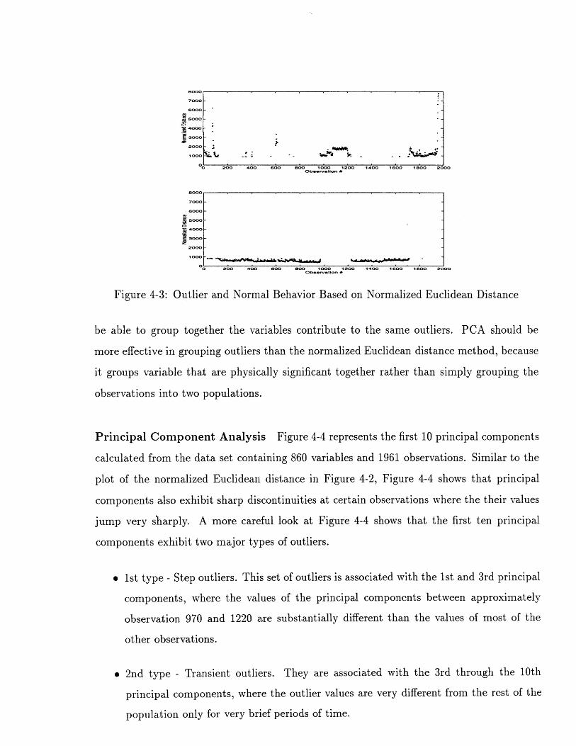
Figure 4-3: Outlier and Normal Behavior Based on Normalized Euclidean Distance

be able to group together the variables contribute to the same outliers. PCA should be

more effective in grouping outliers than the normalized Euclidean distance method, because

it groups variable that are physically significant together rather than simply grouping the

observations into two populations.

Principal Component Analysis Figure 4-4 represents the first 10 principal components

calculated from the data set containing 860 variables and 1961 observations. Similar to the

plot of the normalized Euclidean distance in Figure 4-2, Figure 4-4 shows that principal

components also exhibit sharp discontinuities at certain observations where the their values

jump very sharply. A more careful look at Figure 4-4 shows that the first ten principal

components exhibit two major types of outliers.

* 1st type - Step outliers. This set of outliers is associated with the 1st and 3rd principal

components, where the values of the principal components between approximately

observation 970 and 1220 are substantially different than the values of most of the

other observations.

* 2nd type - Transient outliers. They are associated with the 3rd through the 10th

principal components, where the outlier values are very different from the rest of the

population only for very brief periods of time.

200 48 00 80 00 ro 1200 1400 1600 1800 20 00Obtse ation 0

"7ru~·s~hkut~,*c~,r;~.h+~liirirr3

Observation #

Figure 4-4: First Ten Principal Components of Web Process 2 Data Set

These two types of outliers seem to be controlled by two different set of physical param-

eters. The first type of outliers takes place when the principal component jumps suddenly

from a certain range of value to a different range of values, stays there for a period of time,

and jumps back to the original range of values. The second type of outliers are transient out-

liers that occur abruptly and for brief periods of time. The contrasting behavior of these two

types of outliers indicates that they are controlled by separate underlying physical processes.

Looking at the 3rd through 10th principal components associated with transient outliers,

we can identify two distinct groups within the transient outlier set.

* The first group is associated with the 3rd, 4th, and 5th principal components, where

their values exhibit sharp changes at approximately observations 100, 1750, and 1950

occurring with similar relative proportions.

* The second group is associated with the 7th, 8th, 9th, and 10th principal components,

where their values change sharply at approximately observation 600.

PCA with Frequency Filtering Transient outliers occur when the values of the principal

components abruptly jump to a very different value for a short period of time before returning

to the original values. As discovered from Figure 4-4, there are two kinds of transient outliers

associated with the 3rd through 10th principal components. The figure shows that the 1st

kind of transient outliers is spread out over the 3rd, 4th, 5th, and 6th principal components,

while the second kind is spread out over the 7th, 8th, 9th, and 10 principal components.

PCA collapses variables that are similar to the same dimensions. But in this case, each

of the two kinds of transient outliers are spread out over more than one dimension. One

hypothesis for this phenomenon is that the original data set is dominated by low-frequency

behavior. As a result, the first few principal components are also dominated by low-frequency

behavior, and the high-frequency transient outliers are not dominant enough to be grouped

to the same dimensions.

Since we know that the transient outliers are associated with high-frequency behavior,

one way of collapsing the transient outliers into a smaller number of dimensions is to perform

high-pass filtering on the original data set before applying PCA. The idea here is that with

the low-frequency components filtered out, PCA can group the high-frequency transient

outliers much more effectively.

High-Pass Fil f-gh-Pass F"b

_040.

o;

0.1 0.2 0.3 04 05 06 07 0.8 0.9

o08

0.6

004

0.2

0

Norm F-qouooy (0p0) Noff Fr.quwcy (vpi)

220 1-200 -

FNom FRquency (wp0 Norm FoMquo•y (PON

Figure 4-5: High-Pass Filters with Wp=0.1 and Wp = 0.3

Figure 4-5 shows the graphs of two high-pass filters utilized to remove the low-frequency

components in the original variables. Figure 4-6 presents the first 10 principal components

0 01 02 03 04 05 0 901 02 03 04 05 06 o7 a 0

Jti • 0Fii 1 -

~1 -0064

2000 -. 0 600

-so o

:0 1 w i +on

oi_, :.o .. .•... : :': ... ..,o oo00 1000 00 2000O

20

Cft0,00tjý

--

I, :: ..L... A.$ ".i ,2 - .11 M,.,j'j. 77 "p"7-1-7-irr

201

a I C'~00 15~00 2000010b..ý.Ulon a

I-00c, • " , Mo 600 1000 o 1 00 2000

40 Ob..,stio. 4

20o0 so0 1000 15OO 2000

Ob -Villn 0

-o• soo • doo • •oo 20oObucrvrtlofl #

Figure 4-6: First Ten Principal Components from 90% High-Pass Filterd Data

--2002 0 2

0 So00 1000 1500 2000

0 on

0,O 50 1000 1500 2000

100

0 500 1000 1500 2000

-o 5oo 1ooo 5oo 2000

50 Boo o~IQO 1 640iS M0 Ob50 0tl0n 0Obrlr~vllon

0 oo ~o•° gsoo 2ooo

Obllervrtlon #

20 500 1000 .1500 2000100

0 soo 1000 1500 20000 Obsorvatlon 0

-1°o 5 1000 1500 2000

50 Obsftostl2,1 0

0 50 1000 1500 2000so OblorvstlonOIL I I , 0 m il an

0 600 1000 1500 2000

ObrWstlon 0-a soo • doo ,.oo 2•ooo

Figure 4-7: First Ten Principal Components from 70% High-Pass Filtered Data

-- 0

II

soo 1ooo 15oo 20004DUý.Va(n 0

.___

1-'_ ! - 2

":" :': • -:: •- .. . .. . .. . . .. . .. ::

W00.-- n

__ r--,

-0soo 1000 oo oo 2oS0o .. o

Ob4 e vtlan w

B00 1000 14500 o I000 4 oo 2o00.b tl i

I

I - .

01·,

,1

I

calculated from variables with the lowest 10 percent frequency range filtered out. Figure 4-7

presents the first 10 principal components calculated from variables with the lowest 30%

frequency range being filtered out.

Figure 4-6 and Figure 4-7 show that PCA, obtained from high-pass filtered variables,

does remove the low-frequency behavior but does not effectively separate the different kinds

of outlier behavior. For the two kinds of transient outliers discussed in the previous section,

PCA with frequency filtering still spreads each one of them out over more than one principal

component.

The first kind of transient outlier appears in the 3rd, 4th, 8th and 10th principal compo-

nent in Figure 4-6 where the lowest 10 percent of the variable frequency range are removed.

Although the second kind appear predominately in the 6th principal component, it also

shows up in the 5th and 9th principal components. In Figure 4-7, where 30 percent of the

lowest variable frequency are filtered out, the two kinds of transient outliers appear slightly

better defined. The first kind mostly occupies the 6th principal component, while the second

kind mostly shows up in the 5th principal component.

4.5.3 Identifying Outlying Variables

From a plant manager's point of view, outliers represent shifts and changes in process pa-

rameters that can potentially effect the quality of the end product. As a result, we want

to develop methods and tools to help managers to identify the physics behind these outlier

behaviors. To understand the underlying physics, we need to determine which variables or

combinations of variables contribute to which outliers. This way, we are able to analyze

the variables and determine the causes for the outliers. In this section I will present some

methods to group the variables according their contributions to the outliers.

Transient Outliers Focusing on the transient outliers in the top plot of Figure 4-3, which

does not include the set of outliers from observation 1000 to 1200, we can see there are

mainly 4 regions where the values of the normalized distance jump up suddenly and return

quickly. These 4 regions are located approximately at observation 100, 600, 1750, and 1950.

The goal here is to determine which variables contribute to these different transient outliers

in these 4 regions. One method to find the contributing variables is to find the variables

that also experience sudden changes in values at the same observations corresponding to the

4 transient-outlier regions.

Since a manufacturing data set often contains hundreds of variables, looking at the time

behavior of each variable might be burdensome in determining the causes of transient outliers.

The following procedure is a simpler way to find the contributing variables. For a data set

X;j, where i represents the observation number 1, . . . , n, and j represents the variable

number 1, . . . , m, D is a difference matrix with dimensions (n - 1) x m, whose rows are

equal to the difference between adjacent rows of X. Dij is defined as:

D = X - X- (4.1)

Let M be a row vector of length m where the jth element represents the average of jth

column of the difference matrix D. The 4 transient outlier regions are represented by j=100,

600, 1750, and 1950 respectively. The variables that contribute to region 1 where j=100 are

variables with index i that satisfy the equation Dij >> Mj. The variables that contribute

to the other outlier regions can be determined by using the appropriate j's.

The basic method described here is to determine the variables whose greatest change

between two consecutive observations compared to the average change occur at the same

observations corresponding to the 4 transient outlier regions. Thus, we can determine a set

of variables that contributes to the transient outlier behavior in each of the 4 regions.

Results show that this method is effective in determining the variables that contribute

to the transient outliers in the different regions. Figure 4-8 is a plot of a set of identified

variables that correspond to outliers in region 1 and 4.

Eigenvector Analysis The eigenvectors associated with the principal components reveal

how much each variable contributes to the time-series behavior of the corresponding principal

components. As a result, eigenvectors associated with principal components that exhibit

outlier behavior can potentially reveal the variables that contribute most to the outliers.

* Step Outliers - Since the first principal component represents most of the behavior as-

sociated with the step outliers, the corresponding eigenvector can provide information

6r 300-- i 2

Vmr 874-D 9 2

Var 37 Var 3see

10 0ooo 30oo looo 2100Var 3Se Vmr 370

Vmr a73 Vlr s"•2 2-40 10002000Var 673 Var 3730 0opVa- 376 Var7376

0 1000 .90 100- ICH0 2000'Var070 mrM70 0oloo o~ oo no

Figure 4-8: Variables Identified that Contribute to Transient Outliers in Region 1 and 4

as to the contributing variables. Figure 4-9 represent plots of the first principal compo-

nent and the corresponding eigenvector. As discussed in Section 4.5.1 , we can see that

10

0

2-10

-20

-30

0 200 400 600 800 1000 1200 1400 100 100Observatilon 0

Figure 4-9: The First Principal Component and the Corresponding Eigenvector from Process2 Data

the 1st principal component is dominated by the outlier behavior from approximately

observation 1000 to 1200. The corresponding eigenvector shows that 122 variables are

weighted significantly more than the rest of the variables. These 122 variables are the

main causes for this type of outlier.

4~.

20 - · · · · · · · ·

-bC) · · · --· ·

jkcC"yU,

--2000

* Transient Outliers - With the 122 variables that contribute to the step outliers removed,

the eigenvectors of the correlation matrix and the associated principal components are

calculated for the remaining 738 variables and 1961 observations. Figure 4-10 are the

first 10 principal components, and Figure 4-12 are the corresponding eigenvectors.

,to,

50 .40o oo 100ooo 160 2000 o 500 1000 1500 2000

. .0 O..0arti•, , .40 .t. n 00- I Z20 -

...ff... ° ~ 2~-20,_ 0 7 --10

0 .5 o0 1000 1 . ooo 0 500 1000So 1500 200020 ThbeFrsvti0Tn P i 0ompobentso,, f 8 Vo moo 1000 1500 2000 0 5 00 1000 10 2000Ob2tarvti2on Ob20 0 tb~on SF0:-20- -20h n·tsl-4- So - 1000 '1500 2 -- A ,; Soo 1 500 2000OClrr"Mtla 0 4 3ftratian &

Fiue41:TeFrtTnPicpa opnnsfo 3 aibe

0,,G~ a wItrlabloJA IN~ao 200 400 oo oo00

Varibl Number

d

0 200 400 500 5000-O2 'doobI

0 U1W" I0 200 400 000 500o 20o 4oo 6°° zoo

0 2 Viable Number

0 200 400 00 00Vlriable Number

0.

o 2oo 400 500 500

o •oo 400 Soo Soo

0.1 V 9j

o 200 400 5 oo oo0.2 Valrbia tle o.tbs

G

o 200 400 00 8oo000. Variable b Numlb5

0 200 400 6b00 S00

S 200 400 800 oo0Vriable t~k.Mbtl

Figure 4-11: The First Ten Eigenvectors from 738 Variables

Since the two kinds of transient outliers are spread out over the first 10 principal

components, the variables that contribute to these two kinds of transient outliers are

spread out over the 10 eigenvectors. As a result, Figure 4-12 show that all the variables

are weighted fairly evenly in the determination of the principal components, and it is

hard to determine which variables contribute most to the outliers from examining the

eigenvectors. Eigenvector analysis is not very effective in isolating variables when the

outlier behaviors are spread out over many principal components.

4.6 Variable Grouping

This section addresses the question: how can variables that are related to some common

physical process be effectively grouped together? In order to group or separate variables, it

is very important to have some understanding of the underlying physics of the manufacturing

process. In web process 2, the manufacturing process is divided into subprocesses, where the

output of one subprocess becomes the input of another. The data set contains both control

and quality variables from all the subprocesses. It is reasonable to hypothesize that variables

that are related to the same subprocess are more correlated with each other than variables

from different subprocesses.

The following 3 subsections present 3 methods of variable separation. Section 4.6.1

presents principal component analysis with a focus on examining the associated eigenvectors

calculated from the correlation matrix of the original data. Section 4.6.2 and Section 4.6.3

introduce two methods where some of the noise in the original data set are removed before

performing PCA. Based on the hypothesis that variables related to the same subprocess

are more correlated than variables from different subprocesses, Section 4.6.2 shows how a

more robust correlation matrix can be used to calculate PCA. In Section 4.6.3, variables are

frequency-filtered prior to the calculation of the correlation matrix. Results will show that

these two methods are more effective than standard PCA in capturing the variables groups

within the original data set.

4.6.1 Principal Component Analysis

Principal component analysis groups variables together based on the variables' correlation

with each other. Recall from Section 2.6.3, the ith principal component is a weighted linear

combination the original set of variables obtained from the following relationship:

zi = w!X (4.2)

where w! is the eigenvector associated with the ith principal component, zi, and X is the

original data set.

Equation 4.2 shows that the eigenvectors characterize the weights of variables in the cal-

culation of the principal components, and the eigenvectors reveal which variables contribute

the most to the time behavior of the corresponding principal components. As a result, exam-

ining the eigenvectors obtained from the correlation matrix of the original data can provide

important information as the how the variables are grouped.

-0 200 40 60 o00 - 0 200 400 60 6oVariable Number 0.1 Variable Number

u 0.2O 7l0 200 400 500 000 00 400 600 600

0.2 2 Variable Number 0 0.2 Variable Number

Figure 4-12: First 10 Eigenvectors of 738 Variables

-0. -ht0.05 0 0.05 0. 0.159

- V.1 - b oNumOber .....

-0.1 -0.5 0 0.05 0.1 0.15

-0.1 -0.05 0 0.05 0.1 0.15Variable Numberht1 -18

-0.1 -0.5•0b•N O, 0.1 0.15

-0.1 -0.05 0 0.05 0.1 0.15Variable Number

-0.1 -0.06 0 0.05 0.1 0.15Variable Number

1On Mh 70

10a10*a -0.1 -005 0 0.05 0.1 0.15Variable Number

11o 0.1 -0.05 0 0.06 0.1 0.15Variable Number

-0.1 -0.05 0 0.05 0.1 0.15Variable Number

Va~rible Number

Figure 4-13: Histograms of the First 10 Eigenvectors of 738 Variables

10

11o

lO0e 1oO

Observation Figure 4-12 shows the eigenvectors associated with the first 10 principal

components obtained from the correlation matrix of 738 variables, and Figure 4-13 are the

histograms of the eigenvectors. In Figure 4-13, the symbol 'ht' represents the height of the

middle bar. Since the sum of the area under the bars for each eigenvector is the same, the

height of the middle bar is a good indication of how widely the values of the eigenvectors

are distributed. The plots of the first 10 eigenvector and the associated histograms reveal

that almost all the variables are weighted towards their respective principal components. No

single eigenvector is dominated by a small number of variables.

Interpretation Based on the assumption that variables from the same subprocess are

highly correlated due to their common link to the underlying physics of the subprocess,

variables from different subprocesses should be less correlated. Since the data set contains

variables from many independent subprocesses, it is expected that many of these variables

will be uncorrelated with each other. Consequently, for each eigenvector calculated from

the correlation matrix, there should be variables that make significant contribution to the

associated principal components, and there should also be variables that make little or no

contribution to the associated principal components.

Contrary to the above hypothesis, Figure 4-12 shows that almost all the variables in the

first 10 eigenvectors contribute to some extent to the time behavior of the first 10 principal

components. This is not consistent with the initial assumption that variables from difference

subprocesses should not be correlated and, thus, should not all contribute to the same

principal components. From this, we can conclude that there is a lot of noise in the original

data set, resulting in accidental correlations between variables from different subprocesses.

Thus PCA does not groups the variables as well as it can. Methods should be developed to

improve the signal-to-noise ratio of the eigenvectors so that PCA can better categorize the

variables collected from different subprocesses.

4.6.2 PCA with Robust Correlation Matrix

Ideally, only variables that are from the same subprocess or that are controlled by the same

underlying physics should contribute to the same principal component. Consequently, it can

be assumed that the variables from different subprocesses are correlated mostly by accident,

and the correlation between them can be considered as noise. One method to improve the

signal-to-noise ratio in the eigenvectors of the correlation matrix is to create a more robust

correlation matrix by eliminating some of the accidental correlations between variables.

10,,

A

n dex

Figure 4-14: Magnitude of Correlation Coefficients of 738 Variables in Descending Order in(a) Normal Scale, (b) Log Scale

Method Figure 4-14 shows the magnitude of the correlation coefficients, rij, calculated

from the 738 variables arranged in a descending order both on a normal scale and a log

scale. In order to create a more robust correlation matrix, where some of the accidental

correlations are removed, let E be the cutoff correlation coefficient, where rijjI < E is set to 0,

and Irij I > c maintains its value. Principal component analysis is performed using this more

robust correlation matrix to determine the grouping of th variables.

Results

Cutoff = 0.06 Figure 4-15 are the first ten eigenvectors calculated from the robust cor-

relations matrix where c = 0.06, and Figure 4-16 are the corresponding histograms.

Cutoff = 0.10 Figure 4-17 are the first ten eigenvectors obtained from the robust corre-

lations matrix where correlation coefficients below 0.1 are set to 0, and Figure 4-18 are the

corresponding histograms.

I

r

4 5 I. 16n

0o.1

0 200 400 600 800O . , BooVariable Number

-0.2

0,2 Variable Number

I 0

0- 200 400 600 o800

0 200 400 600 800

Variable Number

-02

Variable Number

0.1

0 200 400 600 8000.1 Variable Number

0.2 Variable Number

0 200 400 600 800

0.2 200 400 600 Boo

-0 2 Variable Number

-- 0 200 400 600 oo

0.2 Variable Number

Variable Number

10 Eigenvectors of Calculated from Robust Correlation Matrix with Cutoff

j10,-0.1 -0.05 0 0.05 0.1 0.15

Variable Number

102 ht 103

-0.1 -0.05 0 0.05 0.1 0.15

V.ariable Number

10' -0.1 -0.05 0 0.05 0.1 0.15Variable Number

-0.1 -0.05 0 0.05 0.1 0.15Variable Number

-0.1 -0.05 0 0.05 0.1 0.15Variable Number

L 102

ht 71

-0.1 -0.05 0 0.05 0.1 0Variable Number

1 ht - 77

-0.1 -0.05 0 0.05 0.1 0

10

Variable Number

10 L-0.1 -0.05 0 0.05 0.1 0

Variable Number

F10

-0.1 -0.05 o 0.05 o.1 0.Variable Number

Figure 4-16: Histograms of the first 10 Eigenvectors Calculated from Robust CorrelationMatrix with Cutoff = 0.06

Figure 4-15: 1st= 0.06

15

.15

f·L

).

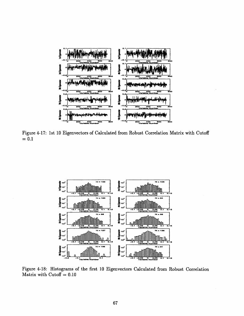
0 2o 0 400 o -0 2 00

0 200 400 o00 800 O 200 400 o00 800Variable Number 0.1 Variable Number

-0.2

-0 200 400 00 800 00 200 400 00 800Variabl Numbr0 Variable Number

0 200 400 600 800 o 200 400 600 800Variable Num•b•r 02 Vaable Number

0.2 0.10 200 400 600 800 - 200 400 600 S002 Varible Number Variable Number

=0.1

10P Lht -103 ht -I n M-10510 10,

10- 28 10-0.1 -0.05 O 0.05 0.1 0.15 -0.1 -0.05 O 0.0 0.1 0.15

Vriablrle Number Va~rible Number

10 [ e 2 10 h O10 10'

-0.1 -0.05 0 0.0 0.1 0.15 -0.1 -0.05 ON 0.0 0.1 0.15V ariable Number Varble Number110o 110

10'i10'

-0.1 -0.05 0 0.05 0.1 0.15 -0.1 -0.05 0 0.05 0.1 0.15Variable Number Variable Number~102 hS- o101 t-0

10 10lo" -V b0r -BA1 .M O 6u OO O1 0 15-0.1 -0.05 0 0.05 0.1 0.16 -0.1 -0.05 0 0.05 0.1 0.15

Variable Number Variable Number10"I ht 127 1 .1, ht - 1310 10'lei In

10 fl. 10-0.2 - 0.1 .- 0.1 -0.05 0 0.05 0.1 0.15

Variable Number Variable Number

Figure 4-18: Histograms of the first 10 Eigenvectors Calculated from Robust CorrelationMatrix with Cutoff = 0.10

· r_

Cutoff = 0.15 Figure 4-19 are the results of eigenvectors calculated from the robust

correlation matrix where E =0.15, and Figure 4-20 are the corresponding histograms.

0 200 400 600 8-0. O . .

S Variable Numbor1

2-o.2 0o o

0. 0Varlbl. Numbe-0r

0 200 400 600 0o1Variabl. Number

0 200 400 600 800Varkble Number

o400 sol 800Variable Number

. Variable Number

00 Va.ab.e Number

Variable Number

Figure 4-19: First 10 Eigenvectors calculated from Correlation Matrix with Cutoff at 0.15

ht - 136

-0.1 -0.05 0 0.05 0.1 0Variable Number

-- 0.1 -- 0.05 0 0.05 0.1 0Variable Number

-0.1 -0.05 0 0.05 0.1 0Var-abla Number

-0.1 -0.05 0 0.05 0.1 0Variable Number

V-IrWab N~umber

.15

.15

.15

15

]s

Ih-0.1 -0.05 o 0.05 0 1 0.15

VariableONuOber

Variable Number

10°

-0.1--0.05 0 0.05 0.1 0.15Variable Nunbar

-0.1 -0.05 0 0.05 0.1 0.15vaftabla N uber

Figure 4-20: Histogram of First 10 Eigenvectors calculated from Robust Correlation Matrixwith Cutoff at 0.15

Cutoff = 0.18 Figure 4-21 are plots of the first 10 eigenvectors obtained from the robust

correlation matrix with cutoff coefficient equals 0.18, and Figure 4-22 are the histograms of

the first 10 eigenvectors.

102,-to'

SI,10,10o

•1oz

10oIla• IO'

2io10

• °|

o.9 o.1

-0.1 200 400800 -o 2o 40 o00 00

Varlabla Numviber VrIable Number

0 200 400 500 500 0 OO 400 000 5000 200 400 500 800 0 200 400 000 500V0rleble Number .VerLeblo NUmber

0 200V- 400 500 -500 20 400 800 500V0rlebi Number Vmrvibie Number

Figure 4-21: First 10 Eigenvectors calculated from Robust Correlation Matrix with Cutoffat 0.18at 0. 18

110

10

-0.1 -0.05 0 0.05 0.1 0.15

10-o -0.1 -o0.00 o 0.o0 0.. 0...

V-6..fta bdurt

-0.1 -O.O6 O 0.0 0.1 0.10

-10

-0.• -0.r05 0 0.05 0.1 0.15

loo

-0.1 -0.05 0 0.05 0.1 0.15

VIl*b N h umbr 1

-0.1 -0.05 0 0.05 0.1 0.15110

-0.1 -0.05 0 0.05 0.1 0.15ve"'U'a "',Z

Figure 4-22: Histogram of First 10 Eigenvectors calculated from Robust Correlation Matrixwith Cutoff at 0.18

69

Interpretation The figures of eigenvectors obtained from correlation matrices with differ-

ent cutoff values show that a more robust correlation matrix is more effective in grouping

correlated variables. As the cutoff values increase, eigenvectors show that the variables that

contribute to the associated principal components are weighted more, while the variables

that do not contribute to the associated principal components are weighted less. In ad-

dition, the histograms of these eigenvectors show that the distribution of the eigenvectors

become increasingly narrower as the cutoff correlation coefficients are increased. As was

discussed before, a narrower distribution means a taller middle bar. The average height of

the middle bar of the first 10 eigenvectors increases from 86.0 to 98.1, to 113.3, to 133.7, and

to 137.8 as the cutoff level increases from 0 to 0.06, to 0.10, to 0.15, and to 0.18. A narrower

distribution means that for each eigenvector, only a small number of variables contribute

to the associated principal component, while most of the variables make minimum or no

contribution to the associated principal component. This is consistent with the hypothesis

that variables from different subprocesses should not all contribute to the same principal

components.

Comparison Figure 4-23 is a comparison of 5 eigenvectors calculated from 5 different cor-

relation matrices obtained from different cutoff values. The plots show that the eigenvectors

calculated using the more robust correlation matrix groups the variables much better than

the eigenvector calculated using the original correlation matrix. One can see that the signal-

to-noise ratio of the values of the eigenvector increases as the cutoff correlation coefficient

level increases.

The histograms of the eigenvectors in Figure 4-24 also indicate the improvements in the

signal-to-noise ratio. The figure shows that the distributions of the eigenvectors get narrower

as the cutoff coefficients are increased. The height of the middle bar increases from 78 to

270 and the cutoff coefficient increases from 0 to 0.18. This means that as the correlation

matrix becomes more robust, accidentally correlated variables are weighted less, while the

significant variables are weighted more.

-o0S0 100 20 30Oe 40 500 800 700

0.2 Observation 7

0 100 200 300 400 500 800 700Observation 5

0.2-0.2

o 100 200 300 400 500 600 700Observation 0

-0 .0100 200 300 400 500 600 700

(b) Robust Correlation Matrix with CutObff0.06 (c) Robust Correlationrvati Matrix with Cut-on0•! o.1 100 200 300 400 500 S0o 700Observation 0

off=0.10, (d) Robust Correlation Matrix with Cutoff=0.15, (e) Robust Correlation Matrixwith Cutoff=0.18

with Cutoff=O.18

-0.2102

-0.2

--0.2

10'

-0.2

10,-0.2

mht - 7 i

-0.15 -0.1 -0.05 Ou r.05 0.1 0.15-0.15 -0.1 -0.0 VariableONumber.0 o O. 5

ht - 10 2

--. 1 2 --. 1 0.o5VarlblONumbr0.OS 0.1 0.15

ht - 123

-0.15 -0.1 -0.05 VadblONum r 0.05 0.1 0.15Variable Number ht - 22-0..15 o -0.05 1 0. 0.05 .0.1

Variable Number ht 1 270

5 -0.1 -0.05 0 0.05 0.1 0.16Va~rible Number

Figure 4-24: A Comparison of Histograms of the Eigenvectors

4.6.3 PCA with Frequency-Filtered Variables

Figure 4-10 in Section 4.6.1 shows that with the exception of transient outliers, the first few

principal components of the 738 variables are mostly dominated by low-frequency behav-

ior. In Section 4.5.2, attempts were made to isolate transient outliers by performing PCA

on variables with the low-frequency components removed. In the previous section, it was

shown the a robust correlation coefficient matrix can be effective in separating variables and

reducing noise in PCA. In this section, we hope the PCA with frequency-filtered variables

can also remove the noise components in the original data set and more effectively group the

variables.

Method Attempts are made to perform principal component analysis after the original

set of variables are frequency filtered. The idea is that we hope that noise can be filtered

out in certain frequency bands, so that PCA can show the same promising results as PCA

with robust correlations with regards to grouping variables.

Frequency-Filters Figure 4.6.3 are samples of a high-pass filter and a band-pass filters

used to remove noise in the original data set.

HDh-Ps F#O .v~p_ F

1

D.;C.C€ ·

-No.m Fnm.0-o y (

4o

(a)

Figure 4-25: (a) High-Pass Filter with Wp =

(b)0.3 (b) Band-Pass Filter with Wp=[0.2, 0.4]

dI · )O 0.1 02 0.3 0.4 .5 Om 47 OA 0.-

N_ f:Mq1WWY Z'0 0.1 02 0.3 0.4 0. 0 0 7 07 oJ O.

0 0 0.1 0.2 013 OA 0.5 0.6 O 0.8 0J I

j

Results For variables that are high-pass filtered with Wp=0.1, Figure 4-26 illustrates

the first ten eigenvectors calculated from the variables' correlation matrix. Figure 4-27 are

histograms of the eigenvectors.

o 200 400 60 600O

0.2 Variable Numb 0r

S0.2 iVlr Clblt Number

-0.2

Figure 4-26: First 10 Eigenvectors Calculated

-I.1 ae "t - 'so nO'

1.0aleumbr

S -0. o.1

-0.1VaablONU O.VartblaeNumbr.1

•oo

VokrlmblO NumbO1•O m h' • "b

* 1 ;·'z1 , 1 - 1x o.:

o ROO 400 S 0ooV.Or:la N. b.:r

O 0 400 000 So00o

o 200 400 Soo o0o

from High-Pass Filtered (Wp=0.1) Variablesoo

from High-Pass Filtered (Wp=0.1) Variables

-o.1 VarablhONumt - 1

-. •Verlablr Numb .1110r

-0.0. o O'V.11.0g. Numb~r

Figure 4-27: Histograms of First 10 Eigenvectors Calculated from High-Pass(Wp=0.1) Variables

Filtered

Figure 4-28 are the eigenvectors calculated from the correlation matrix of high-pass fil-

tered variables with Wp=0.3. Figure 4-29 are the histograms of the eigenvectors.

Figure 4-30 are the eigenvectors calculated from the correlation matrix of high-pass fil-

tered variables with Wp=0.4. Figure 4-31 are the histograms of the eigenvectors.

-- 200 400 600 800 0 200 400 600 Boo0.2 Vriab.e Num-r 0.5 V.b Vab Number

S6 Variabe N.umber Variable Number0. o 2o0 400 Soo S0o 0 200 400 S00 800

0. Variable Number Variable Number

0 200 400 600 800 Eo 200 400 60oo 0e0.5 Varinble Numbe• Variable Num-br

Figiubl N.4-r VFs1E e e r NuCtHere

Figure 4-28: First 10 Eigenvectors Calculated from High-Pass Filtered (Wp=0.3) Variables

... .. ....o . . .. °r . ...S10 ht -1 70

-0 2 -0.1 0 o.1 0.2

Vzrialble Number

0, 1°11 o

[1 0.210e -0.2 -0.1 o o. 0.2Variable Numberht - 170

~~07

1°,N/o . "u [1... . - .i •, .•, e ,.N : ...

ht 1 84

1 -0.2 -0.1T 0 .1 0.2

0.2 -0.1 0 0.1 0.2VI r ble Number

02 hit 1 Ss-0 2 -0. i bON b

0 "10.2

Figure 4-29: Histograms of First 10 Eigenvectors Calculated from High-Pass Filtered(Wp=0.3) Variables

0 2 I R 7 7 V 'Ib e N u br T 0 5V e l b e N m r

-0.0 200 400 o000 o00 200 400 800 Bo000

V.ariable Numb•r Vrl.ble Num.b.r

S200 400 000 000 0 200 400 000 100010 oIO 200 4100 0900 800 - 0 200 4000 000 8000

0. Variablae Number Vartafble Nurrmber

1..1.0~t]0 200 400 600 000 0 200 4o 00 00 oo000.0 200 41000 so Boo 0 200 400 0 0

Vaerable Number Variable Number

Figure 4-30: First 10 Eigenvectors Calculated from High-Pass Filtered (Wp=0.4) VariablesS2 400 Soo -0 0 20 400 Soo BooVmrlabla M.Mbbro Variabla Numbor

Figure 4-30: First 10 Eigenvectors Calculated from High-Pass Filtered (Wp=0.4) Variables

10ht 21

... . .-1r.d.o u o• ..

-0.2• -- o. ... 0. 0o...Vratý, u br".10 * '

10'

lo°

-0.2 -0.1 0 0.1 0.2Vmrlmblý "umbrr10, 4 ý h 40~* 10, rorn

-0.2 -0. 0 . 0.2

0.2z -0.1~ 0 0.1 0.2VlrtrAMw Mumbrr

.10. h,. . N

O -. r .... IuVnl.2Vmr~ablo Mumbrr

roO ht - 2014

10* A f

-0.2 -0.1 0 0.1 0.2

rd ht - 3-40

-0.2 0.1 a 0 0.1 0.2-0.2 -0.1 0 0.1 0.2

V al ht a sb

..•., 1Nu mb n

0. 2 , u -1 0.~_M,

-t oo n I-0.2 -0.1 0 0.1 0.2.Vl m, a Numkr o

--0 "t -- "ai

-02 -01 0 0-" 0.2~.b#ý Pj .,,brr

Figure 4-31: Histograms of First 10 Eigenvectors Calculated from High-Pass Filtered(Wp=0.4) Variables

02.2. 0.2.

Figure 4-32 are the eigenvectors calculated from the correlation matrix of band-pass

filtered (Wp=[0.2, 0.4]) variables. Figure 4-33 are the histogram of the eigenvectors.

O 200 40o o 00 800

O- j I0.2 VadA umber

0.2

-0.20 2Variable NumberO 800o 200 400 .00 8000.2 V..bl.. .Num

o 200 400 Soo 8BooVariable Number

A

0.2 Vraibe MNniib-er

0 200 400 600 SooVar0able Numbar

'''I

IO 200 400 o00 6oo

0. Vrd.14t

O

0 o

200 400 600 8o00Variable Number

0.2 0Variable Number

02

0 200 400 00 800

O0. 20Variablh Numbeo

0 O jý.j~a."gk

Figure 4-32: First 10 Eigenvectors CalculatedVariables

-0f.r 2B0 400 600 8e0Varlable Number

from Band-Pass Filtered (Wp=[0.2, 0.4])

-... -... Var ..... 2 .... 2 . .

lo°

,o·,o hl-137-- 0.2 -0.1 0 O.1 0.2Variable Number

so102 Vo 0.2

-0.2 0*V 0 0. 1

0.2

.... arue Numbe2 to t t --40

loO

_0_1 -0. 0 0"' 0.2V-i-ebl. P4.-t-

M 02ht -1~34

iE0-02 --0.11 0 0.1 0.2

VVriebl. u4-t-

1,.2 ht - 1.40

-0.. -0 1 11 0. 0.2VeIeblý fNumb-r

Figure 4-33: Histograms of First 10 Eigenvectors(Wp=[0.2, 0.4]) Variables

Calculated from Band-Pass Filtered

Figure 4-34 are the eigenvectors calculated from the correlation matrix of band-pass

filtered (Wp=[0.2, 0.3]) variables. Figure 4-35 are the histogram of the eigenvectors.

Interpretation The figures of eigenvectors obtained from the correlation matrices of high-

pass and band-pass filtered variables show that PCA with frequency filtered variables is also

-0.2 ~ ~ t~ -o1 a i bs o u b I100--0.2 -0' 0.1

-02 - .VariableoNumb o.10 .2,M - 3rlo 1

.... ... ri.... Eu...o.1-=o0.2 -0-1 0 0.1-Vsrlblo

Numb-r10 2 M h - 121

•,oo n I--0.2 -0"'-IfbfýNum-ý'

.... ... ~ ~ h -.... o. ...o.w1010

-- 0.2 -- o.1 0 0.1vmrlmbfý Numb-r

tht - 04

ti)

--0.2 -01 0 0.1Var ibleNumbo

v.• I I

0.2 O" T0 200 400 00 oo00 0 200 400 600 600

Var°able Number 02 RVa• b Num•r O

7o 1 Tri Fo !o 200 400 600 600 0 200 400 600 600

0.2 Varibla Number 0.2 able Number0.2 0.2

-0 200 400 00 6200 400 600 000

S VVariables Number Varibl NumberooI IM .-0.2 - Va-" ible Numb. 0" " -- " Vrr"b"Num rc-0.2 . -0.

0 200 400 600 00 0 200 400 o00 00S- -Varable Number 0- Variabl Numb.

Figure 4-34: First 10 Eigenvectors Calculated from Band-Pass Filtered (Wp=[0.2, 0.3])Variables

110 110

V.riable Number Variable Number

ht10 110 t c

10 110-0.2 -0.1 0 0.1 0.2 -0.2 -0.1 0 0.1 0.2

Variable Number Variable Number

Elk nWII-02 -0.1 0 0.1 0.2 -0.2 -0.1 0 0.1 0.2

-0.2 -01 0 01 0.2 -02 -0.1 0 0.1 0.2Varlable Number Variable Number

Figure 4-35: Histograms of First 10 Eigenvectors Calculated from Band-Pass Filtered(Wp=[0.2, 0.3]) Variables

effective in grouping correlated variables together. The histograms indicate that the distri-

butions of these eigenvectors are much narrower than the distributions of the eigenvectors

associated with the correlation matrix of the original data. The average heights of the middle

bars of the first 10 eigenvectors associated with the filtered variables obtained from filters

with normalized pass-band frequency Wp = 0.1, 0.3, 0.4, [0.2, 0.4], and [0.2, 0.3] are 155, 237,

230,128, and 114 respectively. Compared to an average middle bar of 86 for the distribution

of the first 10 eigenvectors of the original data set, the distribution of the eigenvectors from

frequency-filtered variables are much narrower. Consequently, it is reasonable to state that

by removing the noise in the original data set, PCA with frequency-filtered variables im-

proves the signal-to-noise ratio of the eigenvectors, where significant variables are weighted

more, and accidentally correlated variables are weighted less.

Chapter 5

Conclusion and Suggested Work

This thesis presented various methods for analyzing multivariate data sets from continous

web manufacturing processes. The analysis techniques described in Chapter 2 were applied

to two sets of data sets from two different web processes in Chapter 3 and Chapter 4. These

analysis techniques combined with an understanding of the physics of the manufacturing pro-

cesses can produce insights into information-rich data sets. Experiment results show that

both normalized Euclidean distance and principal component analysis are effective in sep-

arating the outliers from the main population. Correlation analysis on Poisson-distributed

defect densities shows the difficulties in determining the true correlation between variables

when the signal-to-noise ratio of the underlying processes are unknown. Principal compo-

nent analysis is a good way to determine the existence of linear relationships between sets

of variables. 'Based on the hypothesis that variables from the same subprocess are more cor-

related than variables from different subprocesses, both principal component analysis with

robust correlation matrix and principal component analysis with frequency-filtered variables

are effective in grouping variables.

Hopefully, the results of my experiments can lead to more research in the area of mul-

tivariate analysis of manufacturing data in the future. Other multivariate methods can be

explored to identify and to treat outliers. In addition, mathematical models can be built to

determine the effects of Poisson noise on the calculation of correlation between processes.

Furthermore, mathematical methods can be developed to quantify the effects of non-linear

operations on the correlation matrices on the removal of noise and on the effectiveness of

grouping variables. Combining a solid understanding of the underlying physics with a mas-

tery of analysis techniques can lead to tremendous progress in the area of data analysis of

manufacturing data.

Bibliography

[1] M.R. Anderberg, Cluster Analysis for Applications, Academic Press, New York, 1973.

[2] T.J. Derksen, The Treatment of Outliers and Missing Data in Multivariate Manufactur-ing Data Massachusetts Institute of Technology, Department of Electrical Engineeringand Computer Science, 1996.

[3] B.B. Jackson, Multivariate Data Analysis, Richard D. Irwin, Inc., Illinois, 1983.

R.J.A. Little, Statistical Analysis With Missing Data, John Wiley & Sons, Inc., NewYork, 1987.

[4] M.A. Rawizza, Time-Series Analysis of Multivariate Manufacturing Data Sets Mas-sachusetts Institute of Technology, Department of Electrical Engineering and ComputerScience, 1996.

[5] A.C. Rencher, Methods of Multivariate Analysis, John Wiley & Sons, Inc., New York,1995.