Multistep Monotone Recursive Methods�

Leonard J. MirmanUniversity of Virginia

Kevin L. Re¤ettArizona State University

December, 2003Preliminary and Incomplete

Abstract

A powerful new class of monotone recursive methods is described forstudying the existence, characterization, and computation of recursivecompetitive equilibrium in a large class of in�nite horizon economies withcapital, production, public policy, behavioral heterogeneity, and incom-plete markets. The analysis combines aspects of topology in normal cones,lattice theory, and interval analysis. The methods are multistep in thesense that recursive equilibrium are computed using compositions of �xedpoint operators. The class of economies studied covers many situationswhere traditional monotone map methods (e.g, Coleman [19] and relatedconstructions) can not be applied, and includes models such as the modelof Bewley [12] and Krusell and Smith [50]. The methods are constructiveand combine aspects of topological and lattice theoretic �xed point the-ory. Discussions of the implications for characterizing the accuracy of ofnumerical solutions to the class of economies is discussed, and some basiccomparative statics results are provided.

1 Introduction

Since the original work of Lucas and Prescott [59], Brock and Mirman [16],and Prescott and Mehra [69], recursive methods and dynamic programminghave become staples in the toolkit of many researchers in macroeconomics, eco-nomic growth, monetary economics and public �nance.1 The methods have

�The authors would like to thank Manjira Datta, Tom Krebs, Olivier Morand, MarioPascoa, Richard Rogerson, and Manuel Santos as well as the participants of the 2003 SAETConference in Rodos Greece for helpful discussions. Re¤ett would like to thank the Dean�sAward in Excellence Summer Research Program at Arizona State for generously funding thisresearch. This is a very preliminary draft of the paper. Do not circulate the current draft,rather email the authors at Kevin.re¤ett@asu.edu for the most recent version.

1The use of recursive methods in economics dynamics has been extensive over the last thirtyyears. See for example, the monograph of Stokey, Lucas, with Prescott [82] and Ljungqvistand Sargent [56] for historical developments and further motivation for the use and importanceof recursive methods in studying economic dynamics.

1

been shown to provide sharp characterizations of recursive (Markovian) equilib-rium in many situations where the second welfare theorem is available. Theseresults have been obtained by applying results in the dynamic programmingliterature of the 1960s in conjunction with the second welfare theorem to pro-vide sharp characterizations of recursive versions of central planning problems.Further given recent developments of lattice programming methods for dynamiceconomies in the work of Amir, Mirman, and Perkins [4] and Mirman, Morand,and Re¤ett [64], monotone comparative dynamics on the space of economiesfor a large class of Pareto optimal economies is also available on the entire setof recursive equilibrium. As numerical solution algorithms based the monotonecontraction mapping theorem for dynamic programming is often available, sharpcharacterizations of numerical implementations of these recursive methods arealso well-known (e.g, Santos and Vigo [78]). Therefore when the second welfaretheorem is available, it has been found that the theory, characterization, andcomputation of recursive competitive equilibrium can be uni�ed to provide avery powerful systematic approach to the study of the structure of Markovianequilibrium in a wide array of Arrow-Debreu-McKenzie settings.Unfortunately, the development of a similar collection of recursive methods

powerful enough to characterize the set of Markovian equilibrium in environ-ments where the second welfare theorem fails has been much more elusive, es-pecially in settings where there is activist or passive public policy (either �scalor monetary), incomplete asset markets, behavioral heterogeneity, and/or mul-tisector production. In homogeneous agent economies with complete marketsand equilibrium distortions such as taxes and production nonconvexities, an ex-tensive set of methods are available. In particular a series of papers over thelast �fteen years has provided a powerful collection of monotone recursive meth-ods based on order-theoretic �xed point theory has been developed. Beginningwith Lucas and Stokey [58], Bizer and Judd [15] Coleman [19], and continuingwith a series of recent developments presented in Greenwood and Hu¤man [35],Coleman [20][21], Datta, Mirman, and Re¤ett [25], Morand and Re¤ett [68],and Mirman, Morand, and Re¤ett [64], a set of monotone recursive methodsthat integrate existence, characterization, and computation of recursive equi-librium has been delivered that uni�es the study of existence, characterization,comparative statics on the space of economies, and numerical approximation ofMarkovian equilibrium.2

Unfortunately, these methods have yet to be extended systematically to com-petitive settings with many agents.3 As many interesting situations studied in

2For some interesting recent nonexistence of Markovian equilibrium results, see Santos [76]and Krebs [48]

3There are two notable exceptions to this statement. First, the methods in Mirman,Morand, and Re¤ett [64] actually work for symmetric equilibrium in some multiagent modelswith incomplete markets and aggregate and idiosyncratic risk (namely models with a �niteor countable number of ex post heterogeneity). More directly though, a recent paper byDatta, Mirman, Morand, and Re¤ett [26], monotone map methods have been extended to thestudy of stationary Ramsey equilibrium problems with public policy (related to the work ofBecker and Zilcha [8]). In this paper, the authors develop order theoretic topological �xedpoint methods based on monotone operators that compute Markovian equilibrium in the

2

applied work in macroeconomics, public �nance, economic growth and develop-ment, and dynamic industrial organization often involve a role for public policy(�scal or monetary), production nonconvexities, and incomplete markets, thisshortcoming has been a serious impediment to unifying theoretical and com-putation approaches to the decentralization of these economies, and the char-acterization of recursive numerical algorithms attempting tied to theoreticalconstructions to construct Markovian equilibrium via successive approximationis essentially nonexistent.4

This paper takes a large �rst step in bridging the gap between theoreticaland numerical implementations of monotone recursive methods. It proposes anew collection of �xed point algorithms capable of unifying topological aspectsof the problem with recent lattice theoretic developments. We then apply themethods to a collection of economies where traditional Monotone Map methodssuch as Coleman [19] are not apparently available. To distinguish our meth-ods from those approaches in the current literature, we �rst present proofs ofexistence of recursive equilibrium based on nonconstructive topological �xedpoint arguments using a version of Schauder�s theorem. In some sense, whileour methods are reminiscent of some existing approaches to the problem in theliterature using local convexity arguments (e.g, Miao [61]), they are also quitedi¤erent. In particular, what is interesting though is that unlike many currentapproaches (e.g, Bergin and Bernhardt [10][11] and Miao [60][61]), we approachto the existence question by studying �xed point constructions on the spaceof candidate equilibrium "policy functions" as opposed to sequences of equilib-rium distributions. This allows us to actually deliver new characterizations ofrecursive equilibrium that are not provided in this recent existing body of work.To avoid a complete reliance on nonconstructive topological methods, our

methods exploit the presence of dynamic complementarities in the underlyingagents decision environment, but in general study these complementarities arean expanded state space. The resulting "multistep" monotone method there-fore in the end is based on an equilibrium version of household Euler equationinequality. The algorithm sequentially computes recursive equilibrium as fol-lows: (i) compute individual decision rules given the aggregate laws of motionfor the aggregate variables via a version of Tarski�s theorem using an "ascend-ing" operator; (ii) exploit well-known comparative statics results for �xed pointcorrespondences in a parameter in conjunction with additional topological reg-

spirit of those consider in the present paper. For these economies, it is shown that successiveapproximation schemes appear available.This extends the results in an earlier paper of Beckerand Zilcha [8] by providing the �rst set of constructive �xed point result on this problem, asopposed to appealing to local convexity arguments.As this paper will discuss, those methods do not appear available for the Bewley-style

models considered in papers such as Aiyagari [6][7], Huggett [42], Krusell and Smith [50], andMiao [60][61].

4There has been much work on methods to provide numerical solutions to dynamic equi-librium models (See for example, Judd [45] for an excellent summary of these methods).Unfortunately, formal arguments concerning the accuracy of these methods have not beenforthcoming (in part because theoretical approaches to studying the existence questions havebeen nonconstructive). For one line of work attempting to rectify this situation for nonoptimaleconomies, see the discussion in Mirman, Morand and Re¤ett [64].

3

ularity conditions to de�ne a second stage operator that can be proven to be acompact antitone operator that are self-maps on a compact subsets of a normalcone )and therefore have a nonempty set of �xed points), and �nally (iii) developa successive approximation algorithm (as an interval iteration procedure) basedupon this compact antitone operator. This last step applies some recent resultsobtained in Re¤ett [73] for compact antitone operators and their relationshipto interval analysis methods presented in Moore [66][67] and Rall [70]. In thislatter step, the unifying construction for understanding successive approxima-tions in either case (monotone or antitone operators) involves view iterations interms of well-known results in the literature on condensing maps.What is clear from our work is that one promising approach to provid-

ing constructive �xed point arguments is to integrate topological constructionsfor compact operators on normal cones with the results for order continuousmonotone operators on complete lattices. As the approach is based on Eulerinequalities in equilibrium, the approach described in this paper needs a settingwhere Euler inequalities (in equilibrium) are both necessary and su¢ cient forRecursive equilibrium. Therefore unlike work based on a pure lattice program-ming approach (e.g, Mirman, Morand, and Re¤ett [64] and Re¤ett [72][71]), weneed enough concavity to obtain su¢ cient conditions for the topological conti-nuity conditions needed for decreasing operators to have a �xed point property.Also, to obtain convergence of our successive approximations, operators in thispaper need to be continuous in uniform topologies. It therefore would seem thatour new approach seems to require a "concave" setting.In a series of papers initiated by the work of Coleman [18][19][20][21], a

large and powerful class of monotone-map methods have been proposed for thecast of continuous Markovian equilibrium. In these settings, the �xed points ofnonlinear operators de�ned implicitly in an equilibrium set of Euler equationshas been developed.5 In many cases, the methods use topological methods toapply order theoretic �xed point arguments using generalizations of the famoustheorem of Tarski [83]. Unfortunately, in many applications using these topo-logical methods, joint monotonicity of both investment and consumption plans(in equilibrium) is needed to �nd suitably chain complete subsets of partiallyordered Banach lattices of continuous functions where an application of Tarski�stheorem is available. (e.g., see in addition to Coleman�s work, Greenwood andHu¤man [35] and Datta, Mirman, and Re¤ett [25] where similar approachesare taken combining topological methods with Tarski�s theorem). In many in-teresting economic environments, such joint monotonicity is not available. InMirman, Morand, and Re¤ett [64], su¢ cient conditions for smooth and Lip-schitzian recursive equilibrium are presented that generalize the Coleman re-sults in many ways. Morand and Re¤ett [68] then generalize the result forsingle agent economies to unbounded state spaces.

5For additional work in this tradition, see Greenwood and Hu¤man [35] Datta, Mirman,and Re¤ett [25], Datta, Mirman, Morand, and Re¤ett [26], and Morand and Re¤ett [68].For a relationship between the lattice theoretic methods of Mirman, Morand, and Re¤ett

[64] and Euler equation methods based upon Coleman [19], see the extensive discussion inDatta et.al [26].

4

Unfortunately, for settings with many agents, few results are known. Theresults in Becker and Zilcha [8] are placed in a monotone operator setting byDatta et. al [26] where the authors provide a method for extending the tra-ditional Monotone Map approach of Coleman�s to a version of the multiagentRamsey economy studied in Becker and Zilcha [8]. As we discuss in section �veof this paper, the methods in this latter paper are not available for the class ofmultiagent economies studied in this paper. In particular, it turns out that inthe models such as Bewley models with incomplete markets, one cannot de�ne amonotone operator on a space of suitably chain complete candidate equilibriumpolicy functions let alone obtain a self-map back to that. Therefore it seemsdi¢ cult to formulate problem as a collection of iterative modi�ed planning typeproblems of a �nite horizon as done in Datta et. al [26].The paper is laid out as follows. In the second section of the paper, we

review the mathematical terminology needed to understand the remainder ofthe paper. Section three then surveys a number of �xed point results that wewill use in the paper, also providing some new results needed in our work. Aswill be clear form reading this section, our �xed point discussion emphasizes thecomputation of the �xed point set. Therefore we have an extensive discussionof �xed point results for isotone and antitone operators in compact subsets ofnormal cones. In section four, we provide an initial presentation of the multistepmethod by proving a new existence and computational result for recursive equi-librium in the homogeneous agent case studied originally in Coleman [19]. Theresult is obtain using our new multistep approach. We compare the structureof the multistep approach to that of the "single-step" Coleman Monotone mapmethod also. In section �ve, we apply our multistep methods to a class of largeeconomies with a continuum of �uctuating agents studied originally in Bewley[12] (also, for cases with Markovian shocks, see Aiyagari [6][7], Huggett [42],and Miao [60]). For these economies, we �rst develop existence argument viaSchauder�s theorem on a space of equilibrium policy functions (as opposed tospaces of probability measures as in Miao [60]). We then show how a multistepmonotone method can compute recursive equilibrium via successive approxima-tion. In this section, we also discuss extensions of the methods to the case ofMarkovian aggregate risk. The latter problem was considered in Krusell andSmith [50] and Miao [61]. An important aspect of this section is that usingour methods, we prove existence of a recursive equilibrium via Schauder�s �xedpoint theorem on the "natural" state space considered in Krusell and Smith [50](as opposed to the enlarged state space considered in work based on Du¢ e, etal [29]. See also Miao [61], Theorem 4 for discussion). This remains true evenwithout the uniqueness of Markovian equilibrium. In Section six, we discuss ourmethods results in terms of a decision-theoretic interpretations, and emphasisthe nature of single-crossing/upcrossing di¤erence properties as discussed in thework of LiCalzi and Veinott [53] and Milgrom and Shannon [62]. This allowsus to suggest possible extensions of our results to nonconcave economies usinglattice programming methods as developed in Mirman, Morand, and Re¤ett[64]. We discuss both cardinal and ordinal conditions. We conclude by relatingour methods to generalizations of the work on error bounds for numerical meth-

5

ods presented in Santos and Vigo [78] and Santos [77], and suggest how thoseresults can be extend to characterize error bounds for numerical solutions forMarkovian equilibrium in large economies. To accomplish this, we discuss theLipschitzian properties of Recursive equilibrium.

2 De�nitions

In this paper, we will make use of numerous di¤erent �xed point constructions.To adequately discuss these arguments, we need to invest in a substantial dis-cussion of relevant terminology in key aspects of lattice theory and topologicalmethods for operators on normal cones. We begin our discuss with some keyconcepts in lattice theory, and then turn to a discussion of relevant topologicalmethods.

2.1 Lattices, Orders, and Mappings

We begin by discussing lattice theoretic notions useful in the sequel. Let Xbe a ground set. If X is equipped with an order relation �X that is re�exive,transitive, and antisymmetric, we say X is a partially ordered set (or Poset).An order interval is a set I = [a; b] = fxja � x � b; a; b 2 Xg: A subset is orderconvex if it is a subset that contains [a; b] whenever it contains a � b: An upper(resp. lower) bound for a set B � X is an element xu(resp. xl) 2 B such thatfor any other element x 2 B; x � xu (resp. xl � x) for all x 2 B: The pair(X;�X) is a lattice if any two elements x and x0 in X , we have in the set X aleast upper bound, denoted x ^ x0; and a greatest lower bound denoted x _ x0:The former is referred to as �the meet�, while the latter is referred to as �thejoin�of two points, x; x0 2 X: The product of a arbitrary collection of latticesequipped with the product (coordinatewise) order is a lattice. A subset B of Xis a sublattice of X if it contains the sup and the inf (with respect to X) of anypair of points in B:A lattice is complete if any subset B of X has a least upperbound and a greatest lower bound. The supremum (in�mum) of B, if it exists,is a least upper bound (greatest lower bound). A chain C � X is a subset ofX for which all pairs of elements are ordered. If every chain in X is complete,then X is referred to as a chain complete Poset. If every chain that is countableis complete, then X is referred to as a countably chain complete Poset.Now consider mappings in partial ordered spaces. We will use the term

mapping f : X ! Y to refer a relational statement between elements of adomain and range. The mapping therefore can be of the form of "set-to-set","point-to-set", or "point-to-set". When f is a point-to-point mapping, we willoften refer to the mapping f as a function or operator between X and Y .For functions and operators, we can de�ne some terms used to characterizetheir monotonicity properties when both X and Y are Posets. Therefore, let(X;�X) and (Y;�Y ) be Posets. An operator f : X ! Y is said to be isotone(or monotone) on X if f(x0) �Y f(x) when x0 �X x for x; x0 2 X: If we have

6

f(x0) >Y f(x) when x0 >X x; then we say the operator f is increasing. Further,if we have f(x0) >Y f(x) when x0 �X x; x0 6= x, we say f is strictly increasing.An operator f(x) is antitone if f(x) �Y f(x0) if x0 �x x: Therefore followingour de�nitions of increasing and strictly increasing, we say an operator f isdecreasing if f(x0) < f(x) when x0 > x: If f(x

0) < f(x) when x0 � x; x0 6= x

then f(x) is strictly decreasing.We can generalize these notations for functions and operators to correspon-

dences (or multifunctions). A correspondence or multifunction will be a "point-to-set" mapping. For the "monotonicity" of a correspondence, we need to extendthe notation of order preserving and order reversing to correspondences. Forour purposes, we only need to consider the case of order preserving correspon-dences. We say a correspondence (or multifunction) f : X ! 2y is ascending inthe set relation S denoted by �S if f(x0) �S f(x) when x0 �X x: We do notrequire the set relation to be a valid partial order, and therefore an ascendingcorrespondence is not necessarily an isotone or order preserving correspondence.To be more precise, consider f :X ! 2Y where 2Y are the powersets of a par-tially order set Y: The induced set relation on the powersets 2Y is the ordering ofthe powersets based upon pointwise considerations implied by the partial orderon Y. We will typically use induced set relations. In some cases, these inducedset relations will imply valid partial orders. (e.g, see the strong set order below).Sometimes this will not be the case (see all of the weak set relations discussedbelow). One reason for considering the case where a correspondence is ascend-ing but not necessarily formally isotone is that requiring valid partial orders onthe powersets 2Y is not necessary for the existence of monotone selections. (e.g,see Smithson [80], and Veinott [85]).In this paper, we will focus primarily on four important set relations, and

only the last two will be valid partial orders on 2Y n?. So say Y is a Poset set,and A;B 2 2Y : We de�ne (i) the V�Weak Set relation �won 2Y : A �w B iffor any a 2 A; b 2 B, either a ^ b 2 B or a _ b 2 A;(ii) the Strong Set Order�a on 2Y : A �a B if for any a 2 A; b 2 B, a ^ b 2 B and a _ b 2 A;(iii)the S�weak set relation r �ason 2Y : A �as B i¤ for any a 2 A; there existsa b 2 B such that a � b; and for any b 2 B; there exists an a 2 A such thata � b; (iv) the Pointwise Strong Set Order �sson 2Y n? : A �ss B i¤ a 2 A;b 2 B; then we have a � b in the partial order structure on A for all a; b:6 Thesefour set relations are used to de�ne an ascending correspondence, but only theset relations �a(the strong set order) and �ss(the pointwise strong set order)induce partial orders on 2Y n?: When a correspondence is therefore ascendingin either of these two set relations, we sometimes refer to the correspondence asisotone. When a correspondence is isotone in any of these set relations on thedual order, we will say the correspondence is antitone. One �nal set relationwe appeal to on occasion on the powersets 2Y is set inclusion. Set inclusioncan be made to be a valid partial order on 2Y . We say a correspondence �(x)

6When considering set relations that actually induce a partial order, we must restrictattention to P (Y )n;: Veinott [85] develops (i), (ii), and (iv). The S-weak set relation in (iii)is studied in Smithson [80]. It has been subsequently referred under a di¤erent name as the�weak induced set order� and characterized in Topkis ([84], p38).

7

� 2Y is inclusive monotone (resp. inclusive antitone) if whenever x1 � x2;�(x1) � (resp. �)�(x2); i.e, � satis�es set inclusion.Finally let A : X ! 2x be a non-empty valued correspondence for each

x 2 X: A special case of the mapping A(x) occurs when A(x) is single-valuedfor each x: When the correspondence A(x) is single valued, we refer to it as anoperator or function. The correspondence � is said to have a �xed point if thereexists a x such that x 2 �(x): Therefore, a function A(x) has a �xed point ifA(x) = x: Let An be the �xed point set of An(x) (a �xed point of the nth orbitof A(x)): For antitone maps, it turns out that the idea of a �xed edge is useful.A �xed apex of an operator A(x) : X ! X is a pair (u; v) 2 X �X such thatT (u) = v and T (v) = u: If u � v, the the pair (u; v) is referred to as a �xed edge.Apparently for any antitone map, a �xed apex has T 2(u) = u; and T 2(v) = v;and therefore u; v 2 A2 : Any �xed point of A(x) is therefore is a �xed edge (ofcourse, the converse is not the case).

2.2 Compact Operators on Normal Cones

Let the ground set X be a real Banach space (a real complete normed vectorspace). An important example of a real Banach space is the space of continuousfunctions x(s) on a compact set S: When X is endowed with a partial order,we refer to X as a partially ordered Banach space. In some cases, if a Banachspace has a norm that is semi-monotonic and possesses a lattice structure, thenX is referred to as a Banach Lattice.A subset E in X a cone i¤ it satis�es the following conditions: (i) E is closed

and convex; (ii) if h 2 E; th 2 E for every t � 0; (iii) if both h and �h are in E,h = 0: We then have h0 � h i¤ h0 � h 2 E; which provides the partial orderinginduced by the cone. In this case, E can be viewed as a Banach lattice underthis partial order. A cone E is normal i¤ there is an element m2 R such thatkhk � mkh0k for any h; h0 2 E; h � h0: A cone E is regular if every monotonesequence in the space is which is order bounded above is convergent. Spacesof non-negative continuous functions X+(S), S compact, with the standarduniform metric/topology and pointwise partial order are normal cones, but arenot regular cones. For example, equicontinuous subsets of X+(S) do have niceregularity properties. (see Dieudonne [28], p. 135 for an extensive discussionof equicontinuity). Spaces of non-negative positive continuously di¤erentiablefunctions X1(S), S compact, is not a normal cone.An operator A:E ! X is continuous if when fxng ! x;A(xn) ! A(x). In

the literature, the de�nitions of "compact" operators di¤er. We shall say anoperator A is compact i¤ it is (i) continuous and (ii) it maps every boundedsubset of E into a relatively compact set in X. This de�nition of a compactoperator which appears in for example Krasnoselskii [46] and Hutson and Pym[44] coincides with a completely continuous operator in other papers in theliterature was cite (e.g., Amann, [3]).

8

2.3 Interval Analysis on Normal Cones

In a series of papers and monographs since the early 1960s beginning with Moore[65], interval analysis has emerged as a new method for unifying the study of�xed point construction and numerical computation using inclusion properties ofinterval mappings. These methods have not found much use in economics, so wewill discuss them in some detail. In particular, we will focus on the applicationof interval methods to operator equations de�ned on compact subsets of normalcones. As these spaces have a lattice structure (actually, are subcomplete inthe Banach lattice C(X); it will turn out that these spaces prove to be naturalspaces to apply interval methods.Let I be an compact order interval in C+(X); and let P 0(I) � 2I be the

subset of all closed order intervals of I: In interval analysis, the interval isthought of as an extension of the idea of a real number. Given this analogy,one can de�ne consider the de�nition of interval arithmetic, and introduce thenotion of an interval mapping from P 0(I) ! P 0(I). Such a set-to-set mappingbegins to capture the notion of an interval mapping. Additionally, using notionsin lattice theory, one can obtain a lattice structure for P 0(I): For example, underthe partial order of set inclusion, P 0(X) is subcomplete in 2I under the relativeorder of set inclusion on the powersets 2I ; 2I a complete lattice.To formalize the notion of a interval mapping (and to characterize its prop-

erties), we need to introduce an arithmetic that is compatible for describ-ing such mappings. In particular, the interval arithmetic systems must have"�" operations that are de�ned on its underlying domains and ranges (where� = (+;�; �; =) that can be used to characterize the interval function. Addi-tionally, one needs corresponding generalized notions of sequences, convergence,norm, etc for interval mappings. In this section we introduce some these basicnotions so we can apply them to characterizations of some of the �xed pointconstructions we consider in section three. We refer the reader to the two mono-graphs of Moore [65][67], Moore [66], and Rall [70] for further discussion of thesenotions.We can generalize arithmetic notions to compact subsets of normal cones

as follows: let the * operations with �={ +,-,�; = } on pairs of real numbers toelements on P 0(X) be de�ned as follows:

A �B = fa � bja 2 A; b 2 B;A;B 2 P 0(I)g

except in the case that 02 B when the operation � is division in which case wedo not de�ne A �B: Following Moore [65], we have the following de�nitions for*={+.-.�; =g on P 0(I)

[a; b] + [c; d] = [a+ c; b+ d]

[a; b]� [c; d] = [a� d; b� c][a; b] � [c; d] = [min(a � c; ad; bc; bd);max[ac; ad; bc; bd][a; b]=[c; d] = [[a; b] � [1=d; 1=c] for 0 =2 [c; d]

9

This arithmetic system is commonly referred to as an interval arithmetic sys-tem. For computational purposes, note that when rounding right endpoints upand left endpoint down, the resulting intervals satisfy set containment. This isreferred to as rounded interval arithmetic.For applying in interval methods to operator equations, we need some ad-

ditional notations. For an compact interval [a; b]; a � b; de�ne the followingnotions respectively of magnitude, width, and midpoint of an arbitrary interval[a; b] which are de�ned respectively as:

j[a; b]j = max(jaj; jbj)w([a; b]) = b� a

m([a; b]) =a+ b

2

We de�ne the intersection of two intervals as their union. This implies

[a; b] [ [c; d] = [min(a; c);max(b; d)]

Intersections are de�ned by

[a; b] \ [c; d] = ? if b < c or d < a= [max(a; c);min(b; d)] otherwise

By set containment, we have [a:b] � [c; d], c � a � b � d:We can discuss one generalization of a monotone map to interval mappings.

Suppose I1; I2 2 P 0([a; b]); and let f : I ! I be a compact operator, and de�nefor the pair (a; b) 2 I � I; the interval operator T : P 0(I)! P 0(I) as T ([a; b]) =[f(a); f(b)]: That is, T is an interval mapping that associates each I 2 P 0(I); andunique element f [I] 2 P 0(f(I)) where the image element f(I) = ff(x)jx 2 Ig: Amap T (I):P 0(I) ! P 0(f(I)) is inclusion monotone if I1 � I2 7! f(I1) � f(I2):The interval map T ([a; b]) is bounded if it takes bounded sets into boundedsets.LetM be a bounded set in a metric space S: The Kuratowski noncompactness

measure �(M) is de�ned to be the in�mum of the set of all numbers � > 0 withthe property that M can be covered with a �nitely many sets, each of whosediameter is less than or equal to �: IfM is complete, theM is relatively compactiff �(M) = 0: An interval operator T :P 0([a; b])! P 0([a; b]) will be said to bek-set contractive if (i) f is continuous and bounded, and there is a number k � 0such that for the implied interval operator T ([a; b]); �(T (M)) � k�(M) for allbounded M: T is condensing i¤ T is bounded and continuous, and �(T (M)) <�(M) for all bounded sets M 2 P 0([a; b]) where �(M) > 0:

3 Fixed Point Theorems and Interval Computa-tion

We begin our discussion with a review of some important �xed point construc-tions that will be applied in the paper. In some sense, the �rst important

10

�xed point result that we should mention that has obviously found an exten-sive application in recursive methods for characterizing Markovian equilibriumfor dynamic economies is the monotone contraction mapping theorem (e.g, seeDenardo [24] for an excellent discussion). In Pareto optimal recursive economies,this result along with the second welfare theorem can be shown to go a longway in characterizing the structure of equilibrium Markovian dynamics. Unfor-tunately, in nonoptimal settings, these results are only part of the story.For such problems, in models with many agents and violations of the second

welfare theorem, topological �xed point theorems have a long history in eco-nomic applications. In this section of the paper although we will discuss someof the particulars of these �xed point constructions (and show how to apply themto nonoptimal settings), we will assume some basic understanding of results inthe areas of convexity, compactness, and continuity. For those interested in aextensive discussion of such matters, we mention the standard references suchas Berge [9] and Rockafellar [74]. Further in this section, we will also provide adiscussion of key lattice theoretic concepts needed in the paper. In particular,as aside from applications of a famous theorem of Tarski [83] lattice-theoretic�xed point constructions have found less use in economics, we will provide aextensive survey of the basic results from lattice �xed point theory that will beused in the paper.

3.1 Nonconstructive Fixed Point Arguments

We �rst consider some important topological �xed point theorems that we willuse in the paper. The �rst theorem we mention is the generalization of Brouwer�s�xed point theorem due to Schauder.7 One will recall the that �xed pointtheorem of Brouwer concerns the existence of a �xed point for a continuousself-mapping from a compact and convex set. Although the theorem is notconstructive, in �nite dimensions from the work of Scarf [79], it is well-knownthat Brouwer�s theorem can in principle be made constructive. Schauder�s the-orem is an in�nite dimensional version of the Brouwer result. Unfortunately,no analog to Scarf�s theorem is available for the in�nite dimensional general-izations such as Schauder or Fan-Glicksberg. We also mention on related �xedpoint constructions are the famous Schauder-Tychono¤ constructions.8 For ourapplications, we will set up applications that only involve Schauder.We now state the version of Schauder�s theorem that we will use in the

sequel. Recalling that an order interval in a normal cone is bounded, closed,

7As in our work, we will use generalizations of Brouwer that involve functions in in�nitedimensional spaces, we will not give a summary of the extensions of Schauder to correspon-dences. We do mention that as the theorem of Kakutani extends Brouwer�s theorem in�nite dimensions to correspondences, work by Fan and Glicksberg generalize the result ofSchauder to correspondences in in�nite dimensions. For a discussion of all of these theorems,see Aliprantis and Border [2] and Zeidler [86].For an application of Fan-Glicksberg in recursive dynamics, see Jovanovic and Rosenthal

[52] and Bergin and Bernhardt [10][11].8See for example, the application of Schauder-Tychono¤ type local convexity arguments in

Becker and Zilcha [8] and Miao [61].

11

and convex, in Proposition 1 we state the following version of Schauder�s result9

Proposition 1 (Hutson and Pym, [44],Theorem 8.3.9). Let E be a cone in areal Banach space X. Suppose E is normal, and let A be a compact operatormapping an order interval [a,b]� E into itself. Then A has a �xed point in[a,b].

Unfortunately, Schauder�s theorem provides only existence results with noguidence for implementation via constructive arguments. When maps are suf-�ciently smooth, degree theory can provide additional characterizations of the�xed point correspondence for the mapping A(x) presented in Proposition 1.To date, this integration of topological degree (and/or homotopy) methods ineconomics has found little application, with the signi�cant applications in thepresent literature only found in the work on smooth di¤erentiable economies in�nite dimensions (or for characterizations in in�nite dimensions, but for optimaleconomies). These methods appear di¢ cult to integrate into a general approachto recursive dynamics of the type studied in the present paper for economieswhere second welfare theorem fails as operators are generally in our work atbest compact Lipschitzian mappings.

3.2 Fixed Points Theorems for Isotone Maps

Instead, we will pursue topological approaches to order theoretic �xed pointconstructions. With this result in mind, we can now state and prove version ofthe �xed point theorem of Tarski ([83], theorem 1). The result we present isclosely related to a key result in Amann ([3], Theorem 6.1) . We add a resultfor our setting on the continuity of the extremal �xed point selections.Let A : I ! I; I = [a; b] � E; E a normal cone. Let A denote the �xed

point correspondence of the operator A: In Theorem 2 we summarize someresults on a compact operator in a parameter in this setting. Much of the proofof (i) and (ii) is found in Datta et. al [26]:

Theorem 2 Let I = [a; b] be an compact subset of positive continuous functionsC+(X) , X compact, and equip C+(X) with the C0 uniform norm and topologyand the pointwise partial order (e.g, C+(X) is a normal cone). Suppose thatA : [a; b]�T ! [a; b], T a compact subset of C+(X), A(x,t) an isotone and com-pact operator jointly in x, and antitone and compact in t. Let A(t) denote the�xed point correspondence of A(x,t) at each t 2 T . Assume that A(t) is strongset order ascending on the dual of T. Then we have the following propertiesfor A(x; t) : (i) for each t, A has a maximal �xed point supA(t) (respec-tively minimal �xed point infA(t)) with supA(t) = limnAn(b) (respectivelyinfA(t) = limnA

n(a)); (ii) A (t) is a complete lattice for each t; (iii) themappings Bu(t) = supA(t) and Bl(t) = inf A(t) are compact antitone oper-ators on T.

9For a formal statement of Schauder�s theorem, see Hutson and Pym [44], theorem 8.2.3).

12

Proof: (i) For the moment, �x t and suppress it in the notion. NecessarilyA(b) � b and, recursively, the sequence fAn(b)g1n=0 is a decreasing sequence ofequicontinuous functions. By the Arzela-Ascoli theorem, there exists a conver-gent subsequence in E. First, since the sequence is decreasing, the convergingsubsequence is the sequence itself.Second, for any k 2 X, the sequence fAn(b(k)g1n=0 is a monotone sequence,

bounded below by a(k), and therefore converges to its inf. Thus, the limitof the sequence fAn(bg1n=0 is infn2NfAn(b)g which we denote bx, and bx 2 E.Further, since a � An(b) � b, then a � bx = infn2NfAn(b)g � b; and bx 2 [a; b].Third, by continuity of A, A( x) = bx which implies that bx is a �xed point.

If x is an arbitrary �xed point in [a; b] such that a � x � b, then for all n,An(b) � x � bx, and therefore bx = inffAn(b)g � x � bx so that x = bx, whichimplies that bx is the maximal �xed point.Finally, since the sequence fAn(b)g1n=0 converges pointwise to a continuous

function, the convergence is uniform by Dini�s theorem (Note that if we relaxthe assumption of compactness of X, then the convergence is uniform on anycompact subset of X). A similar argument yields the minimal �xed point bysuccessive approximation as limnAn(a):

(ii) as the operator A(x; t) is increasing in x for each t; and [a; b] is subcom-plete in E; E a (Banach) lattice, the result follows from Tarski ([83], Theorem1)(iii) We will prove the properties of compactness and antitonicity for Bu(t).

The result will hold for Bl(t) by an similar construction. Fix t 2 T: As thesequence {An(b; t)gn=1n=0 is a is a descending sequence, by the argument in (i), theconvergence of {An(b; t)gn=1n=0 ! supA(t) = Bu(t) is uniform in x for each t:Further as T and X are compact by hypothesis, as {tng ! t, {An(b; tn)gn=1n=0 !fAn(b; t)g uniformly in t, and therefore limnAn(x; tn) = Bu(tn) =supA(tn)!A(t) uniformly in t: Therefore Bu(t) is continuous on T. To prove compactnessof Bu(t) is su¢ ces to show Bu(tn)! Bu(t) is bounded and is an equicontinuoussequence. But as the mapping is continuous on a compact normal cone, thisfollows by Arzela-Ascoli�s theorem, and therefore Bu(t) is compact on T. (Seethe applications of result of Hutson and Pym, [44], Theorem 8.3.17 discussedbelow in Theorem 5). That Bu(t) is antitone follows from Topkis ([84], Theorem2.5.1) �We now consider some �xed point theorems useful for characterizing limiting

distributions for continuous Markov processes. We will need existence theoremsto study the structure of the aggregate environments in which agents are placed,and to justify writing down dynamic programs to characterize agent decisionproblems. As we are also interested in computation via successive approxima-tion, we will also develop some results on computing extremal �xed points foradjoint operators that can be embedded into our �xed point constructions. Forexistence, we appeal to standard existence results (e.g, Futia [38]): For ordertheoretic results, we appeal to results in Bhattacharya and Lee [13], Hopenhaynand Prescott [41], and Huggett [43].To de�ne the setting for our next proposition, let X be a compact metric

13

space, � 2M(X) be a space of �nite probability measures on a X. De�ne thecollection f(x; s) 2 F (x; s) where F (x; s) a consists of all monotone, measurable,continuous maps on X�S endowed with the pointwise Euclidean order. Wethen endow M with the stochastic dominance partial order, that is �0 �M � iffor every monotone, measurable, nonnegative, and bounded function f 2 F = ff : (X� S;�E) ! R+ },

Rf�0(dx � ds) �

Rf�(dx � ds). Hopenhayn and

Prescott ([40];Proposition 3) show that when this order is restricted to thespace of monotone, measurable, bounded, and nonnegative functions, (M,�M )forms a partially order set under the stochastic dominance order �M . Furtherwhen viewed from a topological perspective, Hopenhayn and Prescott ([40],Proposition 4) also provide a metric under whichM is a compact metric space.De�ne the standard adjoint operator J(�; f) : M(X� S)� F ! M(X� S)de�ned as:

J(�; f)(A�B) =ZIA(f(x))�(z;B)�(dx� ds) (1)

For each f 2 F; de�ne the �xed point correspondence for the operator for initial� 2 M(X� S) under the operator J (�; f) to be J(�; f) = f�� 2 M;�� =J(��; f)g. De�ne �m(�; f) = minJ(�; f):We now have the following useful Proposition for studying invariant distrib-

utions associated with candidate functional parameters f for equilibrium. The�rst part of the proposition is a version of a theorem of Abian and Brown [1].The second part is a result for order continuous operators and is from Dugundjiand Granas [30]:

Proposition 3 (i) The mapping J(�; f) is nonempty, and the mapping �m(�; f)is a well-de�ned isotone function in f 2 F ; (ii) if f is additionally continu-ous, and the exists a �0 � J(�0; f); then (a) limn J(�; f) = �m(�; f) and (b)J(�; f) is weakly continuous in f (i.e, if we take fn ! f uniformly, then weobtain J(�; fn) ! J(�; f) in the topology of weak convergence in distribution;(iii) for � 2M; the dynamics {�t(f)gt=1t=0 are monotone for each f 2 F ; andthe dynamics are monotone in f for each �; i.e., if f 0 �F f; �t(�; f 0) � �t(�; f)for all t = f1; 2; :::g where �t(�o; f) = J t�1(�o; f):

Proof: (i) Follows from Dugundji and Granas ([30], Theorem 4.1).(ii) Assume h is continuous. As f is also monotone in (K; z); the adjoint

operator J(�; f) in (3) is isotone in � on M for each f 2 F by a result inHopenhayn and Prescott ([41], Corollary 4)To proceed further, we must �rst de�ne an order continuous operator. We

say an operator J is order continuous if for each countable chain M1 in M;supJ(M1) = J(supM1): See Dugundji and Granas ( [30], p.15). Now for each� 2 E0, for continuous h in (K; z); as (i) � satis�es a Feller property, (ii)h continuous, the adjoint operator is therefore continuous in the topology ofweak convergence (e.g, see Stokey, Lucas, and Prescott [82], Theorem 9.14 andAliprantis and Border [2], Theorem 18.14.3 ). As we have �0 � J(�0; h) for eachf 2 F; and as every chain in M has supremum (Hopenhayn and Prescott, [41],Proposition 1), we conclude thatM has the property for every countable chain.

14

Therefore, the hypotheses of a theorem in Dugundji and Granas ( [30], Theorem4.2) are now satis�ed, and we conclude (a) the �xed point correspondence J(f)is nonempty for each f , and (b) the function mapping �m(f) can be constructedvia successive approximation as �m(f) = min� �

�(f) for each f such that �0 �J(�0; f): A dual argument constructs the maximal limiting distribution in M.To see �m(f) is isotone; take f 0 � f; f; f 0 2 F: Notice that conditions C.1

-C.3 developed in Huggett [43], p9) are satis�ed, and therefore by Huggett ([43], Theorem 3) , we have monotone dynamics i.e., J(�; f 0) �M J(�; f): Thenthe fact that �m(f) = min J(f) is isotone on F follows from order continuityand a corollary in Hopenhayn and Prescott ([41], Corollary 3).(iii) The monotone comparative dynamics result follows from Huggett ([43],

Theorem 3). �In Proposition 4, we turn to the more general case of a mapping A(x; t)

that is actually a correspondence (i.e., multifunction) in (x; t). In this setting,the focus of our discussion is on lattice-theoretic constructions. In some setting(e.g, when the order interval I = [a,b] is a compact subset of a normal cone E,as in Theorem 2 (iii), we will have extremal selections of the correspondenceA(x; t) forming compact monotone selections of the A(x; t): In this case, we canintegrate topological �xed point constructions tightly within a computationalframework based upon Amann [3] (For constructive arguments in settings with-out su¢ cient order continuity, see Echenique [31]).Let 2X denote the powerset of X; X a complete lattice, T a partially order

set, and consider a mapping A:X�T ! 2X that is strong set order ascending in(x; t): We can state two sets of known results concerning such a correspondenceA(x; t). The �rst result is a generalization of Tarski�s theorem to a settingwhere the mapping A(x; t) is an ascending correspondence in the strong setorder in (x; t); the second result provides a monotone comparative static resultin the strong set order for the �xed point correspondence A(t) associated withA(x; t). We refer the reader to Zhou ([87], Theorem 1) and Topkis ([84], 2.5.1)for proofs of (a) and (b) respectively:

Proposition 4 Veinott ([85], Zhou [87], Topkis [84]). Let X be a completelattice,T a partially ordered set, A(x; t) : X�T!X a correspondence that isascending in the strong set order �a on X�T , A(x,t) nonempty, closed, andcomplete-latticed valued for each (x; t): Further, the set of monotone selectionform a complete lattice. Let A(t) denote the set of �xed points of A(x; t) foreach t 2 T: Then (a) A(t) is a nonempty complete lattice for each t, and (b)A(t) is ascending in the strong set order with the set of all monotone selectionsin A(t) a complete lattice.

3.3 Interval Methods for Computing Fixed Points of Com-pact Antitone Operators in Normal Cones

We begin this section we a discussion of the �xed point structure of antitonemaps. In general, decreasing or antitone maps on complete lattices do not have

15

a �xed point property. In when the complete lattice is an equicontinuous subsetof a normal cone and the operator is compact, the situation is di¤erent. In thenext proposition, we review some well-known properties of antitone maps oncomplete lattices. For the sake of our conversation, in Proposition 5 considerthe complete lattice under consideration to be an compact order interval in anormal cone.

Proposition 5 Let A(x,t):[a; b]�T ! [a; b] be a compact antitone operator,

[a,b]� X a compact order interval in a normal cone X, T a partial orderedtopological space. De�ne An(t) to be the �xed point correspondence of An(x,t)in x for each t2 T; and �A(X;t) : T! 2

(X�X) to be the set of �xed edges forA(x,t) in x at t 2 T;�A(X;t) � PA(X;t); PA(X;t) the set of �xed apexes ofA(x,t):X � T ! X. Then we have the following: (i) A(t) is a nonemptyantichain in 2X for each t 2 T; (ii) �A([a; b];t) is nonempty with a minimalpoint a0([a; b]; t)=inf{x2 [a; b]jx � A2(x; t)g and maximal point b0[a; b]; (t) =supfx 2 [a; b]jx � A2(x; t)g; and PA([a:b]; t) is a nonempty complete lattice inthe in the powerset 2[a;b]�[a;b]:

Proof: (i) That A(t) is nonempty follows from our version of Schauder inProposition 1. We then have A(t) an antichain follows from a result in Dacic([22], Proposition 1.1).(ii) That �A([a; b]; t) is nonempty follows from a result in Dacic ([23], The-

orem A). The existence of the minimal and maximal element follows from Dacic([23], Theorem A). That PA([a; b]; t) is a complete lattice follows from Tarski([83], Theorem 1) noting that A2(x; t) (the second orbit of A(x; t) in x) ismonotone in x as A(x; t) is antitone in x for each t by hypothesis. �In theorem 6, we present a collection of new results for antitone compact

maps on normal cones. The methods also use interval analysis to unify the re-sults on inclusive monotone iterative procedures and iterations on isotone/antitonemaps on lattices and Posets. The computation aspects of the theorem are provenusing interval operators on the interval powersets of a compact order interval[a; b] in the normal cone of continuous functions. One interesting aspect of thisresult in the theorem is (ii) where we provide a set of su¢ cient conditions toconstruct �xed points for order reserving maps via successive approximationalgorithms based in inclusive monotone interval operators. These results usinginterval analysis to study computational aspects of the theory are presentedin more detail in Re¤ett [71][73]. Here, we summarize the pertinent resultsfrom these papers that will prove useful for our particular questions concerningmultistep �xed point methods. When reading theorem 6, recall that existenceof solutions for the mapping under consideration follows immediately from theversion of Schauder�s theorem quoted in Proposition 1. The key additional re-sult shows that under some basic regularity conditions on normal cone we study(namely compactness), successive approximation schemes for antitone operatorsconstruct elements in a nonempty �xed point set.

16

Theorem 6 Let E be a normal cone in a real Banach space X, D� E a compactsubset. Let A:D! X be a compact operator (function), A the set of �xed pointof A(x), and assume that there is an order interval [a,b]� D such that b�A(b);A(b) � b: Then (i) A:[a,b]! [a; b]; (ii) if A(x) is antitone, the there exists aninterval iteration inclusion monotone procedure K2(X) : P

0([a; b]) ! P 0([a; b])such that limnKn

2 ([a; b])! x� 2 A;(iii) if A(x) is isotone, then there exists ainterval iteration inclusion monotone procedure K1(X) : P

0([a; b]) ! P 0([a; b])that limnKn

1 ([a; b]) = a� � P 0([a; b]):

Proof: ( i). Follows from the de�nition of an antitone operator and notingthat a � b in the subset D � E:(ii) We �rst note that from an initial order interval [a; b]; and de�neK0

2 ([a; b]) =[a; b]: As A(x) is antitone, there exist sequences a0u = (a;A(b); A

2(a); A3(b); :::gand b0d = (b; A(a); A

2(b); A3(a); :::g that are monotone increasing and decreas-ing respectively to a minimal or maximal �xed edge (a1; b1) where b1 = A(a1)(each of which exists by Proposition 5.ii) : If A(a1) = b1 = a1; then we are done.So say (a1; b1) is a �xed edge of A(x), but not a �xed point. Then we haveA(a1) � a1 necessarily.Set K1

2 ([a; b]) = [a1; b1]; a compact subset of [a; b]: As [a1; b1] is an order in-terval, it is order convex, and therefore by then continuity of A(x) and the inter-mediate value theorem proven in Guillerme ([36], corollary 2), there exists an a

0

1

such that A(a1) � A(a0

1) � a0

1 � a1. De�ne a1u = (a1; A(b1); A2(a1); A3(b1); :::gand b1d = (b1; A(a1); A

2(b1); A3(a1); :::g. Again these are monotone increasing

and decreasing sequences respectively whose limits are a �xed edge (a2; b2) whereb2 = A(a2). We have either a2 is a �xed point, or (a2; T (a2)) a �xed edge. Ifthe latter is the case, set K2

2 ([a; b]) = [a2; b2]: Iterating on the interval operatorKn2 ([a; b]); we have the following monotone inclusion (on the dual of P

0([a; b])Kn2 ([a; b]) � Kn+1

2 ([a; b]) with limnKN2 ([a; b]) = limn \Kn

2 ([a; b]): Note that theexistence of a �xed point (as a compact order interval) for limnKn

2 ([a; b]) thenfollows from Darbo�s �xed point theorem for condensing maps (Zeidler, [86],Theorem 11.A).The �xed point set for an antitone map A(x) by Proposition 5.i is an

nonempty antichain. Further, for the interval iteration procedure Kn2 ([a; b]);

for each iteration n > 0; the set of �xed edges has a minimal and maximalelement: Therefore, all that remains to show is the limiting compact set oflimnK

n2 ([a; b] is a singleton c

� 2 A. We observe that this statement can beshown to be equivalent to having limnan = limn bn = c� (for if this is the case,then by the implication of convergence we have the following: when n odd, wehave pointwise jAn(b(x)) � An�1(a(x))j ! 0 for each x; and n even we haveAn(a(x))� An�1(b(x)) ! 0; therefore both limnan and limnbn share the samelimit c�(x) 2 A by Darbo�s theorem)This last argument takes place in two stage. First, note that as [a; b] � D;

D compact (equicontinuous) on X, X is compact, pointwise convergence impliesuniform convergence by the compactness of A(x). This implies that using thesuccessive approximations {An(an(x))g and fAn(bn(x)))g that de�ne Kn

2 ([a; b]), that limnKn

2 ([a; b]) converges uniformly to a �xed edge [a�; b�] where additional

17

this limiting �xed edge is additionally a �xed point. By the regularity propertyof compact order interval [a; b], as this interval iteration procedure Kn

2 ([a; b]) isbased on a compact operator in a compact subset of a normal cone, all monotonesequences in the relatively compact set A([a,b]) are actually convergent, this bya standard argument (e.g. Hutson and Pym ([44], Theorem 8.3.17). So wehave limnKn

2 ([a; b]) ! I� = [a�; b�] 2 P 0([a:b]) uniformly. But as for each n;Kn2 ([a; b]) = In 2 P 0([a; b]) is based on a antitone compact map, by proposition

5.1, all the �xed points of A(In) � In form an antichain in [a; b]: Therefore thelimit I� must also be an antichain. But by de�nition both endpoints of I� arealso �xed points, and therefore c� = I�; c� a singleton:(iii) Follows from part (ii) of the theorem noting that we can take a1u =

(a;A(a); A2(a); ::::) and b1d = (b; A(b); A2(b); ::::) and that by a theorem inAmann ([3], Theorem 6.1) this successive approximation scheme will convergeto a lower and upper �xed point respectively. Therefore let K�

1 ([a; b]) = limnKn1 ([a; b]) = [a�; b�]=A�where a� and b� are the minimal and maximal �xed

points of A respectively, and A� is the largest �xed point on P 0([a; b]).�A few remarks on theorem 6. Theorem 6 does not deliver uniqueness of

solutions, rather it simply gives conditions under which successive approxima-tions on an order reversing map computes an actual �xed point. For uniquenessconditions, one needs stronger forms of monotonicity or concavity of the op-erator A(x) (and the resulting interval operators K(([a; b]): In particular, forsituations where maps have strong concavity and monotonicity properties, seeKrasnoselskii ([46], Theorems 6.3 and 6.4); for situations where operators canbe shown to be pseudo concave and k0�monotone, see Coleman ([19], Theorem8). Second, to apply the theorem to the construction of Recursive equilibrium,one needs to show that this limit of the decreasing sequence is not a "trivial"equilibrium (e.g, everyone follows an "invest everything forever" decision rulein equilibrium). This situation with trivial �xed points can often be ruled on ineconomic applications.

4 Homogenous Agent Economies

We begin with an illustration of our multistep methods in an economy whereboth "one-step" and "multistep" methods work. In presenting our multistepapproach, aside from using the homogeneous agent setup to introduce the meth-ods, we will actually prove a new existence and computation result not foundthe work of Coleman [19], Greenwood and Hu¤man [35], or Mirman, Morand,and Re¤ett [64].10

10 In all this existing work on Monotone Map Methods, the shocks z are typically assumed tobe countable. In this case, one can obtain compact subsets in the space of continuous functionsby only studying the monotonicity properties of candidate equilibrium for investment andconsumption in K for each z: If z is on a continuous state space, these arguments fail toestablish the requisite equicontinuity. Our argument here though shows this does not matterrelative to the question of existence and computation. See also Erikson [32] for a discussionof these issues in the context of stochastic OLG models.

18

Consider the economy studied in Coleman [19] and Morand and Re¤ett [68].Time is discrete and indexed by t 2 T = f0; 1; 2; :::g, and there is a continuumof in�nitely-lived and identical household/�rm agents facing identical lifetimeitineraries (both ex post and ex ante). For simplicity, in each period, householdsare endowed with a unit of time, which they supply inelastically to competitive�rms.11 Uncertainty comes in the form of a �nite state, �rst-order Markovprocess denoted by zt 2 Z, with stationary transition probabilities �(z; z0): Letthe setK� R+ contain all the feasible values for the aggregate endogenous statevariable K, i.e., the per capita capital to labor ratio, and de�ne the productspace S : K� Z. Since the household also enters each period with an individuallevel of the endogenous state variable k, the individual capital to labor ratio,we denote the state of a household by the vector s = (k; S) 2 K� S.For each period and state, the preferences are represented by a period utility

index u(ci), where ci 2 K � R+ is period i consumption. Letting zi = (z1; :::; zi)denote the history of the shocks until period i, a household�s lifetime preferencesare de�ned over in�nite sequences indexed by date and history c = (czi) andare given by:

U(c) = Eo

( 1Xi=0

�iu(ci)

);

where the summation is with respect to the probability structure of the shocks.We make the following assumption:

Assumption 1. The utility function u : K 7! R is bounded, twice con-tinuously di¤erentiable, strictly increasing, strictly concave. In addition, u0(c)satis�es the standard Inada conditions:

limc!o

u0(c) =1 and limc!1

u0(c) = 0:

It proves convenient for our latter application of multistep methods to Be-wley models to study the economy described in Coleman [19] as opposed tothe one described in Greenwood and Hu¤man [35] and Mirman, Morand, andRe¤ett [64] where a reduced-form production function is used.12 This choiceof convention in decentralization is chosen simply to allow use to make explicitthe di¤erences in the complementarity structure of agent decision problems thatunderlies a single-step vs multistep method. Assume the production functiongiven to a large number of identical �rms is f(K; z); that rental price of capital

11A similar algorithm can be developed for models with elastic labor supply as in Datta,Mirman, and Morand [25]. For the models in section three and four, it is not clear how toextend the multistep method for the inelastic labor supply case.12Greenwood and Hu¤man [35] discuss how results for economies discussed in this section

actually apply to a much large set of economies where one writes down a reduced from distortedproduction function. That is, for both the single-step and multistep methods we consider inthis section, similar arguments can be shown to allow one to study many other economies with�scal and monetary policy (e.g., state contingent taxation, activist policy, value �at money viacash-in-advance or money in the utility function, etc), models with production nonconvexities,monopolistic competition. We refer the reader to their paper for a extensive discussion.

19

and wage rates are given by r(K; z) = f1; w = f2; and that household income inthe current period depends on government capital income taxes at rate (K; z);and lump-sum transfers it back to households according to J(K; z): That is,de�ne household incomeThe underlying technology is assumed to exhibit constant returns to scale

in private inputs of capital and labor, and satis�es the following assumption.

Assumption 2(i). f(K; z) = 0 for all K 2 K; z 2 Z.(ii). f is continuously di¤erentiable, strictly increasing, strictly concave in

its �rst argument, and limk!0f1(K; z)!1(iii). r(K; z)=(1- (K; z))f1(K; z) is strictly decreasing and continuous in

K for each z and preserves the Inada condition in K in (ii) for each z:(iv) There exist k(z) > 0 such that f(k(z); z) = k(z) and f(K; z) < k for

all k > k(z) and for all z 2 Z � R++, Z compact.

The restrictions on the primitives in Assumptions 1-2 are entirely standardin the nonoptimal stochastic growth literature (e.g., Brock and Mirman [16]and Greenwood and Hu¤man [35]). We note we can easily relax the boundaryconditions (e.g, Inada conditions on u and f ) for existence of a complete latticeof Markovian equilibrium at the expense of uniqueness. (See Mirman, Morand,and Re¤ett [64], section 5 for proof). Assumption 2(iv) is a standard featurein stochastic growth literature (See Brock and Mirman [16]), and implies thatsupz k(z) exists. As a consequence, the state-space for the endogenous variablek (and for output) can be taken to be the compact intervalK = [0; �k]; where �k isthe larger of the two quantities, the initial stock k0 and supz k(z). This impliesthat the boundedness assumption on utility can be relaxed, since a continuousutility de�ned on a compact space is necessarily bounded.The dynamic decision problem for the household can now be described. We

de�ne the household�s feasible correspondence �(s) for the distorted economyas the set of actions (c; y) satisfying the following constraints:

�(s) = fc; yjc+ y � f(K; z) + (k �K)r(K; z) + J(K; z); and c; y � 0g

Under Assumption 1, �(s) is a continuous, compact and convex valued, non-empty correspondence for each s = (k;K; z) 2 K� S. Also, the correspondence� is expanding in (k;K; z); i.e, �(s) � �(s) when s �E s0:Let C(KxZ) = C(S) be the space of continuous maps h : S ! R, S =

(K; z) 2 S compact. Endow C(S) with the C0 uniform topology, the standardpointwise partial order (e.g, h0 � h if for all S; h0(S) � h(S)): It is well knownthat C(S) is a Banach lattice. If we de�ne C+(S) to be the space of positivecontinuous functions, then C+(S) is a normal cone (see Krasnoselskii, [46], p20).We can construct the household�s decision problem. Assume that house-

holds assume they live in an economy where the per capita capital stock evolvesaccording to:

K 0 = h(K; z);

20

where h 2 H0(S) = f h(K; z) : S! K , h 2C+(S) and measurable such that (i)h(K; z) is increasing in K; each z ; and (ii) f(K; z)� h(K; z) is increasing in Keach z g. De�ne a subset of H(S) � H0

(S), H0(S) = fh 2 H0j h and (f �h) arejointly monotone in (K; z)g

In lemma 7, we summarize what is known about the spacesH(S) andH0(S) :

Lemma 7 (i) H(S) is a compact order interval in C+(S) in the C0 uniformtopology; (ii) H(S) is subcomplete in the Banach lattice of continuous functionsC(S); (iii) H0(S) is a compact order interval in C+(S) and subcomplete in C(S)if Z is discrete.

Proof : (i) See Coleman ([19], Proposition 3) noting the with z 2 Z � R++,equicontinuity in z for the space follows from h and (y � h) increasing in z (ii)See Morand and Re¤ett [68], Theorem 1); (iii) Coleman ([19], Proposition 3).�We make two remarks on lemma 7 and its relationship with the continuation

of our arguments in this section. First, notice that when Z is discrete, H0(S)is the space of equilibrium policy functions considered in Coleman [19][21] andGreenwood and Hu¤man [35]. This space is only equicontinuous (and therefore acomplete lattice) if Z is a discrete random variable. Therefore the results we willprove using a multistep method will be new, and extend the existing results onexistence and computation of recursive equilibrium to the case where the shockstake values in a continuous state space. Second, in Mirman, Morand, and Re¤ett[64] the authors provide su¢ cient conditions for recursive equilibrium to existin the space H(S) when the state space for Z is continuous. Those conditionsappear very strong relative to the results obtain using multistep methods in thelast part of this section, and require additional dynamic complementarities toexist in the economies underlying primitive data in situation where the shocksof Markovian. What we do therefore using the multistep method is prove theexistence (and uniqueness) of recursive equilibrium in the space H0(S) eventhough we do not have joint monotonicity in both investment and consumptionin (K; z) as required in the paper by Mirman, Morand, and Re¤ett [64]. Thisthen becomes a �rst step in obtaining our results for the Bewley models ofsection 5.We can now consider a description of household decision problems for a re-

cursive competitive equilibrium for this economy. As in the next section theshocks are assumed to be discrete, assume as in Coleman [19] that the agenttakes as given h 2 H0(S). Then the dynamic decision problem facing a typi-cal household is summarized by the solution J(s;h) to the following Bellmanequation:

v(s;h) = sup(c;y)2�(s)

fu(c) + �ZZv(y; h(K; z); z0)�(z; dz0)g: (2)

Standard arguments (e.g, Coleman [19], Proposition 1) show the existence of av(s; h) 2 V for each (k;K; z; h) that satis�es this functional equation, where V is

21

the Banach space of bounded, continuous, real valued functions that are concavein their �rst argument when endowed with the pointwise partial order and thesup norm (see, for instance, Stokey, Lucas and Prescott [82]). In addition, it canbe shown that J is strictly concave in k, and solution for optimal consumptionare interior for all h 2 H0 given the Inada conditions. Therefore one can alsoapply the argument in Mirman and Zilcha ([63], lemma 4) to obtain a standardenvelope theorem for v(s;h), i.e, J is once di¤erentiable in k.The de�nition of recursive competitive equilibrium follows as in Prescott and

Mehra [69]. That is, we de�ne an equilibrium for the state contingent incometax economy as follows:

De�nition: A (recursive) competitive equilibrium for this economy consistsof a value function for the household J(s); and the associated individual deci-sions c and k0 such that: (i) J(s) satis�es the household�s Bellman equation(1), and c; k0 solve the optimization problem in the Bellman�s equation givent; (ii) all markets clear: i.e., k0 = h(S) = K 0and (iii) the government budgetbalances.

4.1 Computation using a Coleman Approach

For the sake of comparison for later discussion, �rst consider the traditional"single-step" method of Coleman [19]. To apply Coleman�s argument for theeconomies under consideration, we must �rst restrict attention to the case wherez 2 Z; Z discrete. In this method, we �rst rewrite the equilibrium version of thehousehold Euler equation into a form that can be shown to correspondence witha decision problem where agent "best responds" to their own future consumptiondecision with a current consumption decision. This procedure de�nes a nonlinear�xed operator as an implicit mapping in the Equilibrium Euler equation. Onenice feature of this approach is if one takes next period consumption to beall of output f(K; z); then the trajectory of this nonlinear operator can beassociated with a collection of modi�ed planning problems each possessing inincreasing di¤erences between the controls for consumption and investment andthe parameters (K;h): That is increasing di¤erences in the sense of the Topkis-Veinott theory of supermodular functions (in this case in (c; h)) that generatesColeman�s monotone operator on the space H0 from the initial consumptionh0 = f . The complementary between consumption, investment, and aggregatecapital stock therefore then creates a self map back to H0:13

For the details, consider an equilibrium version of the household�s Eulerequation (which is necessary and su¢ cient for the existence of a Recursive com-petitive equilibrium as v�(k;K; z; h) that solves (1) is concave in k for each(K; z; h)): Following Coleman [19], a recursive equilibrium is any consumption

13See Mirman, Morand, and Re¤ett ([64], section 5) for an extensive discussion of theColeman Monotone Map algorithm in the language of lattice programming and superextremaloptimization.

22

function h > 0 ; h(K; z) = h(K;K; z) such that

u0(h(K; z))��Zu0(h(f�h(K; z); z0)f1(f�h(K; z); f�h(K; z); z0)�(z; dz0) = 0

De�ne the operator Ach(K; z) for h 2 H = (fh(K; z)j0 � h(K; z) � f(K; z); hnondecreasing in K for each z such that f�h increasing in K each zg as follows

Z(x;K; z;h) = u0(x)� �Zu0(h(f � x; z0)f1(f � x; z0)�(z; dz0) (3)

Ach = fxjZ = 0 if h > 0 for all (K; z); 0 else}

One can easily check the following comparative statics on the equation Z(x;K; z; h) :(i) Z is strictly decreasing in x for each (K; z; h) such that as x ! 0; Z ! 1;and as x ! f; Z ! 1; (ii) continuous and increasing in h for each (x;K; z)(where continuity in h follows from the compactness of the space H in theuniform topology); (iii ) is continuous and increasing in K for each (x; z; h):Therefore (i) and (ii) imply Ach is a continuous monotone operator on H0,

and (i) and (iii) imply that Ach is continuous in K for each h: Noting the secondresult, we can then obtain the following inequality:

u0(Ach(K 0; z) � u0(Ach(K; z)

= �

Zu0(h(f �Ach(K; z); z0)�

f1(f �Ach(K; z); z0)�(z; dz0)

We therefore conclude from (4) that Ach must be such that f�Ach is increasingin K: Therefore Ach 2 H0: Compactness of the operator then follows from thecontinuity of the operator Coleman ([19], Proposition 4), noting that Ac : H0 !H0 so all sequences in the range are bounded and equicontinuous (which issu¢ cient for compactness via the Arzela-Ascoli theorem).Therefore as the operator Ach is a monotone compact self map in H0; by

Theorem 2 in our section 2, there exists a successive approximation schemebased on Ac(f) that will compute the maximal �xed point of Ach: The minimal�xed point is trivial, and is h = 0: We also remark the by the main theoremin Coleman [21], the set of strictly positive solutions to Ach� h = 0 is unique,and there consist of the only recursive equilibrium in H0. Following the argu-ments the in Mirman, Morand, and Re¤ett ([64], section 5.2), we then have thestrongest form of monotone comparative statics/dynamics on the set of recur-sive equilibrium for the distorted equilibrium. For example, using a version oftheir main monotone comparative dynamics theorem (e.g., see [64], Theorem 9),one can easily show using their argument that if f 0 and f are two productionfunctions, and their associated distorted factor prices for capital are r0 and r;then any perturbation of f or policy parameters such that r0(K; z) < r(K; z)for all (K; z); equilibrium consumption h(K; z; r0) � h(K; z; r) for each (K; z)

23

(and the ratio of consumption to investment also rises in the pointwise Euclid-ean order). One such perturbation takes in assumption 2(iii) 0(S) � (S) in apointwise order for all S 2 S:

4.2 Computation via a Multistep Interval Method

We now compute this set of recursive equilibrium in H(S) (not H0(S)) using amultistep monotone recursive algorithm. To obtain these more general results,for this section we now let the shock take values in a continuous state spaces, i.e,z 2 Z; Z� R++ compact. Notice that the equilibrium version of the householdEuler equation associated with the dynamic program in (1) can be rewritten tode�ne a new operator Ah as follows:

Z(x;K; z; p; h; ~h) = u0(x)� �Zu0(h(f � x; z0)r(f � ~h(K; z); z0)�(p; dz0) (4)

whereA(h; ~h; p) = fxjZ = 0; h > 0; ~h 2 H0; 0 else} (5)

where we imagine studying the equation in the end when p = z:We �rst observe�rst the (unique) root of Z(x;K; z; p; h; h) = 0; denoted as x�(K; z; p; h; ~h )(where uniqueness follows as Z is strictly decreasing in x, x an element ofa chain K): Additionally, we remark that Z(x;K; z; p; h; ~h) has the followingcomparative statics that will prove useful in describing the behavior of its uniqueroot x�(K; z; h; ~h) : Z is (a) continuous and strictly decreasing in (x; z) foreach (K;h; ~h; p) (b) increasing and continuous in h for each (K; z; p; ~h); (c)decreasing and continuous in ~h for each (K; z; ; p; h); and (d) strictly increasingand continuous in K for each (z; p; h; ~h): We can therefore conclude about theoperator A(h; ~h ):

Lemma 8 (i) A(h; ~h ,p) in (6) is increasing in h for each ~h ; (ii) A is decreasingin ~h for each h; (iii) A(h; ~h) 2 H for each ~h; (iv) A(h,�h) is jointly compact in(h; ~h)

Proof: (i) That A(h; ~h) is isotone follows from the comparative static prop-erties (a) and (b) noted above for Z: (ii) follows from the comparative staticproperties (a) and (c) noted above for Z; (iii) The A(h; ~h)(K; z) has the neededmonotonicity properties in K for each z follows from the comparative staticproperties (a) and (d) noted above for Z: To show f �A is also increasing in Kfor each z, using a similar argument to Coleman�s, we note that for each pair(h; ~h); we have

u0(Ah(K 0; z0; ~h) � u0(Ah(K; z; ~h)

= �

Zu0(h(f �Ah(K; z; ~h); z0)

� f1(f �Ah(K; z; ~h); z0)�(p; dz0)

24

where implies A(h; ~h) must be such that f � A(h; ~h) is increasing in (K; z) foreach p = z: Therefore we conclude A(h; ~h) 2 H for each pair (h; ~h):For the joint compactness of A(h; ~h) �rst notice A(h; ~h )2 H0: Let (hn; ~hn)!

(h; ~h ) (uniformly in (K; z)). To prove A(h; ~h) is compact it is su¢ cient to proveA(hn; ~hn) is bounded and equicontinuous. As it is easily seen that A(h; ~h) iscontinuous (e.g, Coleman [19], Proposition 4), this results then follows from thecompactness of S and the order interval H0 �H0 by the Arzela-Ascoli theorem.�We now �rst prove existence applying the version of Schauder�s theorem

presented in Proposition 1.

Theorem 9 The exists an h� 2 [hl; f ] � H(S); h� > 0; such that h� is aRecursive Competitive equilibrium.

Proof: We then h = ~h; A(h) is continuous on the compact set H. Compact-ness of the operator follows the fact that H is a compact subset of a normalcone (see the application of Hutson and Pym, Theorem 8.3.17 in theorem 5),and A(h) is continuous on H. That there exists a restriction of A(h) to [hl; f ]where A(h) is a self map follows from a standard argument in Coleman [19][21]: namely that A(h) (or a an operator de�ned using the the global inverse trans-formation of the operator A(h) based on the equilibrium marginal utility ofconsumption) as described in Coleman [21]) is k0�monotone and pseudo con-cave, and therefore one can always �nd a function hl 2 H; hl > 0 such thatthere does not exist a �xed point 0 < h� � hl; and A(hl) � hl: �Unfortunately the proof in Theorem 9 is not constructive and di¢ cult to

interpret computationally. We now remedy this problem by proving existenceof equilibrium in two steps, and then using that method to compute equilibrium.Let A(~h) be the �xed point correspondence associated with multistep operatorA(h; ~h): De�ne Bu(~h) = supA(~h ) and Bl(~h)=infA(~h). In Theorem 10, weprove the following successive approximation result based on our Theorem 5:

Theorem 10 (i) A(~h; p) is a nonempty complete lattice such the its extremal�xed points coincide with the compact antitone operators Bu(~h) and Bl(~h); (ii)The sequence {Kn2 ([H(S);p])gn�0 ! h1 converges to a recursive competitiveequilibrium h1 when p = z; (iii) in the case where u0(c)f1 is increasing in z,the limiting distributions the equilibrium dynamics can be constructed as thelimnJn(�0; f)! �1:

Proof: (i). The compactness of A(h; ~h) jointly in its arguments follows froma standard argument uses the fact that S is compact, h; ~h 2 H; H compact,and the continuity result in lemma 8(i) and 8(ii) respectively. Also by thecomparative statics on Z in (4) discussed in (a)-(d) above , by lemma 8.i, A(h; ~h)is isotone in h for each ~h; and by lemma 8.ii A(h; ~h ) is antitone in ~h for each h:

25

Then by theorem 2 (ii), for each ~h; the �xed point correspondence of A,denoted by A(~h) is a nonempty complete lattice (and therefore have extremalelements). By Theorem 2.i the extremal elements of A(~h) can be computedby successive approximation from the points hl = 0 and h = f respectively. ByTheorem 2.iii, the operators Bu(~h) = supxA(

~h) and Bl(~h) = inf A(~h) arecompact operators. Finally the fact that Bu(~h) and Bl(~h) are antitone followsfrom the result of Veinott and Topkis on �xed point comparative statics notedin Proposition 4(b).(ii) Follows from Theorem 6 (ii) noting that the limit h�(K; z; z) satis�es the

following functional equation:

u0(h�(K; z; z) = �

Zu0(h�(f � h�(K; z; z); z0)f1(f � h�(K; z; z); z0)�(z; dz0)

and therefore the recursive competitive equilibrium is the function h(K; z) =h�(K; z; z) =2 H(S):(iii). Follows from Proposition 3(i) and Mirman, Morand, and Re¤ett ([64],

Section 5.3).�To obtain uniqueness, notice that following the arguments Coleman�s ar-

guments that A(h; ~h ) is pseudo concave and k0 monotone in h for each ~h inthe case that u(c) is CES. In this case, Bu = Bl; and then given separabilityof the space H; sequences in H have unique limits, and then Theorem 9 de-livers a unique equilibrium. In the more general case, one can easily recoverthe de�nition of the operator A(h; ~h) from another operator based on the mar-ginal utility of consumption as in Coleman [21]. Therefore A(~h) can then beshown to be single valued for h > 0: Then following the same construction asabove, we arrive at similar uniqueness conclusions as Coleman [21] Finally, bythe strong monotonicity properties of the operator A(h(x); p) near h = 0; wecan �nd a function cl 2 H(S) such that following the construction in Theorem6.iii, we can construct an interval iteration procedure Kn

1 ([cl; f ]; s; �) such thatlimnK

n1 ([cl; f ])!h�(x; s,�) = h(x) > 0 (See Coleman, [19], Theorem 7).

5 Models with a Continuum of Consumers

We now ready to apply our multistep methods to situations where the single-step methods of Coleman [19] are di¢ cult (if not impossible) to apply. We �rstconsider Bewley models without aggregate risk (e.g, See Bewley [12] , Huggett[42], and Miao [60][61]). We then extend the methods to models with aggregateshocks (See Krusell and Smith [50]). For these models, when examining thestructure of equilibrium versions of household Euler inequalities, it will becomereadily apparent that single-step monotone map approaches will prove di¢ cultto apply in these cases. The key features of the models are that there exista continuum of ex ante identical agents facing a standard income �uctuationproblem, they have access to a single asset, there is no borrowing, and there areincomplete markets to insure that all sources of risk. Therefore although agents

26

are ex ante identical as in Brock and Mirman [16] and in Coleman [19], thereare also ex post heterogeneous.We �rst remark that for all of these models considered (and actually the

much large class such as those with Markovian idiosyncratic and aggregate risk),questions pertaining to existence have been addressed via topological arguments.For example, the questions of (i) existence of sequential equilibrium, and (ii) theexistence of stationary Markovian equilibrium has already been resolved. Forexample, su¢ cient conditions for the existence of sequential Markovian equilib-rium on a space of probability measures is also known for Miao ([61], Theorem2), as is the existence of payo¤ equivalent Recursive equilibrium for every se-quential competitive equilibrium ( Miao ([61], Theorem 3). For the case of noaggregate shocks, Miao also proves the existence of a non-trivial invariant dis-tribution (Miao [60], Theorem 3.7). So existence per sa is not the focus of ourcurrent discussion, although the structure of the state space where Recursiveequilibrium exist will be an issue.

5.1 Bewley Models with No Aggregate Risk

In this section, we study a version of the model described in Bewley [12]. Theenvironment has become a workhorse in applied macroeconomics, and has beenstudied in papers such as Aiyagari [6] [7], Huggett [42], and Miao [60] [61].The version of the model we study is a special case of the one found in Miao[60][61]. We �rst study the case without aggregate risk, and then discuss howour arguments apply for the case of aggregate risk associated with technology.There are three key developments in our work that complement the results foundin Miao�s [60][61]: (i) we provide a set of su¢ cient conditions under which thereexists a constructive �xed point argument for computing and characterizing thestructure of Recursive equilibrium on a space of policy functions (as opposedto aggregate distributions); (ii) we study the problem allowing for a role forpublic policy (e.g, taxation and subsidies for capital, nonconvexities in aggregatetechnologies, value �at money, etc); (iii) we prove the existence of a recursiveequilibrium for equilibrium policy functions de�ned on a "natural state space"that consists of current period asset holdings k, current period individual statesof the individual s, and the current state of the aggregate economy (which willtypically be represented by a probability measure � and perhaps a state ofaggregate technology z).There could be potentially very important when exploring the computa-

tional implementations of our work. The space where Markovian equilibriumexistence are Lipschitz continuous, but as the �xed point is computed as thecomposition of operators in parameters, one cannot conclude the �xed point isactually Lipschitz. Using arguments characterizing solutions to Kuhn-Tuckerconditions found in Gauvin and Janin [33], it seems possible to provide thisadditional characterization in some cases. When recursive equilibrium are alsoLipschitz, as our approach can be placed within the context of a dynamic pro-gramming algorithm on a natural state space associated with a value function

27

that is strongly concave, in principle this allows for the possibility of extend-ing the result of Santos and Vigo [78] and Santos [77] to a much large class ofeconomies with incomplete markets and aggregate risk. As for the last result (iii)pertaining to existence and computation of recursive equilibrium on a "naturalstate space", this result is important as in the case of aggregate shocks we aretherefore able to prove the existence of recursive equilibrium on the state spaceconsidered in Krusell and Smith [50] even without uniqueness of equilibrium.One should therefore compare this result for example to a related result in Miao([61], de�nition 3, and theorem 4 ). The key to obtaining this improvement overMiao�s results can be tied to the how we handle the parameter space for agentdecision problems in our economy.To �x ideas, let time be discrete t = f0; 1; 2:::g: There is a continuum of ex

ante identical agents i 2 [0; 1] distributed according to Lebesque measure � whoface a standard income �uctuation problem summarized by stochastic process(sit)t�0 that is Markovian, s 2 S � R+; S compact. They each have accessto a single asset which for simplicity we will think of as capital ki � 0: Weallow no borrowing.14 Latter in this section, we shall consider the case wheretechnology is subjected to an aggregate shock (zt)t�0: In this case, we assumez 2 Z, Z countable in R++: Let K� R+ denote a compact to speci�ed latter,but included in the speci�cation of the state space.Agents have lifetime preferences that are summarize by two identical objects:

a bounded concave continuously di¤erentiable period felicity function ui(c) =u(c) and a discount rate � 2 (0; 1): Lifetime preferences for i 2 [0; 1] are the

U i(ci) = E0

(t=1Xt=0

�tu(cit)

)

where ci = (cit)t�0. Agents enter a period with asset holdings ki and in aparticular state si: De�ne �0(K1 � S1) = �(i 2 [0; 1] : (ki; si) 2 K1 � S1;K1 �S1 2 B(K)�B(S)) where B(X) are the Borel sets of X:We �rst consider the case of no aggregate risk: Let M(K�S) be the space

of �nite probability measures on the support K�S; with � 2 M a typical el-ement. Production takes place according to a "distorted" production functionf(k; n;K�; N�) which is constant returns to scale in its �rst two arguments,and where the equilibrium distortions are assumed to depend on the meaninput levels. A typical �rm chooses (k; n) subject to a factor costs and thepair (K�; N�) = (

Rki�(di);

Rsi�(di)) = (

Rk�(dk � ks);

Rs�(dk � ks)) where

(K�; N�) represent mean capital and labor respectively for a given distributionof agent "types" �:

14Borrowing can be easily incorporated into our methods for the no aggregate risk caseby following the lead of Miao [60] and introducing an ad hoc borrowing constaint into theanalysis. This ad hoc borrowing constraint is critical for existence of continuous Markovianequilibrium (See Krebs, [48]). To keep exposition simple, we study the Bewley case, anddo not allow borrowing. In this sense, the results can easily be shown to apply to the purecurrency models of Lucas [57].

28

De�ne the class of economies � 2 E to be those that satisfy the followingassumptions:15

Assumption 3: The economies � 2 E consist of sets (U;F; �;Q; ki0; si0) suchthat(i) ui = u(c) 2 U if �-a.e i : ui(c) is strictly increasing, strictly concave, C2

over the interior of K such that ui(0) = 0; bounded, and ui0(0) = 1,1< i =� limc!1 log(u

i)0(c)= log(c) <1;16(ii) f 2 F has f(k; n;K�; N�) constant returns to scale in (k; n), strictly in-

creasing, strictly concave in the �rst two arguments, C1 in all arguments, suchthat f1(K; 1;K; 1) is strictly decreasing in K; and satis�es f(0; 1;K�; 1) = 0;fij � 0;limk!0f1(k; 1;K; 1) =1; limk!1f1(k; 1;K; 1)! 0; limn!0f2(k; n;K; 1)!1 for all K 2 K;(iii)f such that y = f1(k; 1;K�; 1)k + f2(k; 1;K�; 1)s is increasing in K�

17 ;(iv) �i 2 (0; 1);(v) (ki0; s

i0) = (K0;s0)� 0;

(vi) the history (sit)t�0 is drawn from Q(s; ds0) 2 �(S) which is a stationarytransition function such that (i) Q(S1; �) is measurable, (ii) Q satis�es standardFeller properties (if f(s; s0) any real-valued, bounded, continuous function ,then

Rf(s; s0)Q(s; ds0) is continuous on S);and (iii) Q satis�es no-conditional

aggregate uncertainty condition18 .

Versions of assumption 3 are found in the literature. Part (i) is the typicalregularity condition on period utility functions, but does not impose bounded-ness (so it allows for power utility). Part (ii) is a version of the boundednessassumption on Greenwood and Hu¤man [35], and implies that the equilibriummean capital stock will lie in K. Assumptions (iii) and (v) are standard. As-sumption (iv) is similar to a stronger assumption made in Becker and Zilcha [8](where in addition they require income to be concave in K�). Assumption (vi)is a standard assumption, and is needed to show the extremal �xed selectionsof our "�rst stage" �xed point maps similar to A(h; h) in Section 4 are compactmeasurable operators in the uniform topology.

15These are essentially assumptions 1-8 in Miao [61] excepting at this stage we have noaggregate shocks and assumption (iii).16First, we will now suppress the notation for i in the primitive data unless clari�cation is

need. Also, see Miao ([60], footnote 6 and Remark 2) for discussion of this formalization ofthe Inada conditions and regularity conditions on u(c).17Miao [60][61] does not make this assumption. It is not clear it is necessary for our meth-

ods to work either. We use it to get su¢ cient complementarity to map back to a space ofLipschitzian functions where the Lipschitz bound is constructed from the joint monotonicityproperties of consumption and savings. But all this is needed is to prove either consumptionor investment is Lipschitz. We will discuss how this assumption might be dispensed with insection 5 of the paper, and suggest methods for relaxing this assumption based on the workof Gauvin and Janin [33].18See Miao [61], Assumption 6 and related discussions for the exact formalization of this

condition, and Feldman and Gilles [37] and Bergin and Bernhardt [10] [11] for a discussion ofits applications to constructions of useful laws of large numbers. .

29

5.1.1 Choice of Parameter Space

We approach the equilibrium problem di¤erently than Miao [61]. Miao�s ap-proach to recursive equilibrium (including the case of aggregate shocks to tech-nology z) can be characterized as follows: (i) characterize a parameter space ofcandidate recursive equilibrium using sequences of distributions � =(�t(zt)t�0where zt is a history of aggregate shock realizations in the a space of in�nite se-quences of probability measures valued inM(K�S) in the in�nite cross-productof these spaces indexed by histories zt;(ii) characterize individual decision prob-lems taking these sequences as given using dynamic programming to computeeach agent i 2 [0; 1] decision rules; (iii) aggregate decision rules using a version ofthe no-conditional aggregate uncertainty decomposition suggested in Bergin andBernhardt [10][11] and Feldman and Gilles [37] to aggregate to construct the im-plied aggregate "response" to the given parametric distribution; (iv) constructa �xed point argument using a local convexity argument (Schauder-Tychono¤)to prove the existence of a �xed point; (v) use this construct to develop pay-o¤ equivalent representations associated with his equilibrium notation (whichin general cannot be deliver a Recursive equilibrium on the "natural" statespace for these problems (e.g, Aiyagari [6][7] and Huggett [42]).19 A recursiveequilibrium is therefore a stationary distribution for these random aggregatedistributions �(z) is indexed by the state of aggregate technology z 2 Z (whichof course in the no aggregate shocks case is a single distribution with z = 1 forexample for all histories).We propose a di¤erent approach, but require more structure. Fortunately

many interesting cases in the literature process our additional structure. Ourmethod proceeds in the following steps: (i) describe a collection of candidateequilibrium policy functions h 2 H on a natural state space (k; s; �); (ii) calcu-late the implied aggregation to distributions under each element of the class Husing a standard result based on Schauder for the existence of �xed points tothe adjoint J(�0; h) for �0 2M implied by the initial capital stock ko;(iii) giventhe collection of parameters describing candidate equilibrium policy functionsH, construct of agent dynamic program for each parameter; (iv) construct amapping whose �xed points via our version Schauder�s theorem in Proposition1 delivers existence of recursive equilibrium on the natural state space; (v) spe-cialize the production functions to allow our multistep methods of section 4 tobe applied to this class of models; (vi) consider an application of a standard lim-iting distribution argument via the theorem of Abian and Brown [1] discussedin Proposition 3 of Section 2 for the operator J(�o; h) where �0 is a degeneratedistribution that places all probability mass at the initial distribution of capitalk0 for constructing a stationary Markov equilibrium.Therefore, in the end, we show via a �xed point argument that we can make

individual decisions consistent (when aggregated) consistent with some elementof the collection of candidate parameters describing the recursive equilibrium

19We should note, in Miao [60], only the stationary equilibrium is constructed. In thatpaper, he uses a di¤erent (but related) method to study the existence of stationary Markovianequilibrium. For our purposes, his arguments in Miao [61] are more pertinent.

30

for each element of the class of economies � 2 E. One critical aspect of ouralgorithm is we avoid the problem discussed in Kubler and Schmedders [51] andMiao [61] by our choice of parameter space for this class of economies.We have assumed a recursive version of the economy studied in Miao [61].

So let current distribution of assets be given as � 2 M: De�ne household in-come to be a mapping y(k; s; �) = y(k; s;K�) = rk +ws where the dependenceof income on � takes a very simple form under constant returns to scale as-sumptions in Assumption 3(ii): We assume �rms maximize pro�ts and underconstant returns to scale, �rm pro�ts are zero so we have r(�) = r(K�; N�) =f1(Rki�(di);

Rsi�(di)), and w(�) = w(K�; N�) = f2(

Rki�(di);

Rsi�(di)): We

normalized the process for the idiosyncratic shocks such that we can use the equi-librium restriction

Rsi�(di)=1. 20 Under our assumptions, when �0 � � under

stochastic dominance, we have r(�0) � r(�); w(�0) � w(�); and y(k; s; z; �0) �y(k; s; z; �):Let (K;K) and (S;S) be measurable spaces, and de�ne C(K� S�M) =

C(X); x = (k; s; �) 2X, X compact, to be the space of continuous measurablemaps h(x) : X ! R;. Endow C(X) with the C0 uniform topology and thestandard pointwise partial order (e.g, h0 � h if for all S; h0(x) � h(x)): Asin section 4, de�ne C+(X) to be the space of positive continuous functions.Therefore C+(X) is a normal cone. To construct the typical decision problemof household i 2 [0; 1], say each household assumes agents that each householdin the economy ex ante make decisions:

K 0 = h(k; s; �)

where h 2 H(X) � C+(X); where

H(X) = fhjh(x) : X!K is continuous, measurable, (6)

isotone in x such that y(x)� h(x) is isotone in xg

Recalling lemma 7 in section 4, it is clear that H(X) has very nice properties.In particular, H(X) (i) is a subcomplete in the Banach lattice C(X); and (ii)is a compact order interval in the normal cone of continuous functions C+(X):Also notice that all elements of H(X) are Lipschitz continuous, and thereforesmooth in the sense of Clarke [17].We now note some basic properties of the adjoint operator when parameter-

ized by elements h 2 H(X): Endow M(K�S) with the stochastic dominancepartial order, that is �0 �M � if for every monotone, measurable, nonnegative,and bounded function l : (K�S;�E) ! R+ ,

Rf�0(dk � ds) �

Rf�(dk � ds).

Hopenhayn and Prescott [41] show that when this order is restricted to thespace of monotone, measurable, bounded, and nonnegative functions, (M,�M )forms a partially order set with a closed order �M . Endow M(K�Z) with the20This assumption is not restrictive in the no aggregate risk case. In the case with aggregate

shocks considered in the next section, we cannot make this normalization. In that case, thestructure of our arguments can be shown not to change, so we will follow Miao [61], assumption5(b) for this case.

31

weak �topology, then M is also a metric space.21

Consider a standard de�nition of an adjoint operator J(�; h)(A � B) :H�M(K�S) ! M(K�S) for Borel measurable sets (A;B) in measurablespaces (K;K) and (S;S) as follows:

J(�; h) =

ZIA(h(k; s; �))Q(s;B)d�(dk � ds) (7)

Because of the assumptions on Q concerning Feller properties, the adjoint op-erator J(�; h) have the following properties: for each h 2 H; J(�:h) is (i) it isweak� continuous in � when viewed as mappings from M(K�S) ! M(K�S)(e.g., Stokey, Lucas with Prescott [82], Theorem 12.3); (ii) when fhng ! h(uniformly) in H(X), the operator J(�; hn) = IA((hn(x))Q(s;B)�(dk � ds)! IA((h(x))Q(s;B)�(dk� ds) = J(�; h) weakly (See using the Lebesque Dom-inated Convergence theorem, Stokey, Lucas, and Prescott ([82], Theorem 9.14),and Aliprantis and Border ([2], Theorem 18.14); (iii)

RkiJ(�; hn)(dk � ds)

!Rki(h)J(�; h)(dk � ks); (iv) if J(h) is the �xed point correspondence for

J(�; h); J is nonempty (Aliprantis and Border, Theorem 18.18). We will usethese facts often in our work in this section. Also notice, that we can character-ize the �xed points of J using the order theoretic �xed point theory describedProposition 3. This will prove especially useful when studying the limiting dis-tributions associated with equilibrium policies h� 2 H:

5.1.2 Household Decision Problems

We now characterize the household�s dynamic program when facing an aggregateenvironment h 2 H; � 2 E. Consider a household entering the period instate x = (k; s; �) 2 X facing an aggregate economy with aggregate dynamics(and prices) summarized by a function h 2 H and in situation (k; s; �). Thevalue function for the household is a function v�(x; h) that is a solution to thefunctional equation:

v�(x;h) = supc;y2�(x)

fu(c) + �ZZ

v�(y; s0; J(�; h))Q(s; ds0)g

where the feasible correspondence �(x) = fc; yjc + y � y(x); c; y � 0g: Inorder to study the existence of a v� that satis�es the above functional equation,consider the operator BC :

BCv(x;h) = supc;y2�(p)

fu(c) + �ZZ

v(y; h(K; z); z0;h)�(z; dz0)g (8)

21Let ffng be a countable set in C(K��) including the unit function. A metric then forthe weak

0�topology on M(K��) is de�ned by

�(�; �0) =j=1Xj=0

jRfjd��

Rfjd�

0j1 + j

Rfjd��

Rfjd�0j

32

where BC is de�ned on the space Vc ={ v(x;h) : X�H!R, v bounded in x,isotone in x for each h; continuous in k and concave in k: Equip Vc with thestandard C0 topology (and the associated uniform metric) and the pointwiseEuclidean partial order. Then Vc is a complete metric space. Lemma 11 providesa �rst set of results characterizing the unique function v� that satis�es (4):

Lemma 11 For � 2 E; h 2 H, (i) BCv � Vc; (ii) there exists a unique v� 2 Vcthat satis�es (8); (iii) the �xed point v� is strictly increasing x and strictlyconcave in k for each h2 H.

Proof: The proof of the lemma is now standard at this stage of the literaturefor economies � 2 E. Claim (i) can be proven using the arguments in LeVanand Morhaim [54] (Theorem 1) but with continuity of the value function ink handled as done in Miao( [60], Theorem 3.1). The second claim then canbe shown to follows also from these two theorems cited above that generalizethe results obtain via standard case of a monotone contraction argument inDenardo [24] to dynamic programming problems with potentially unboundedreturns without using the standard contraction mapping argument. The �nalclaim can be shown by a modi�cation of a standard argument in Stokey, Lucas,with Prescott ( [82], corollary 1, p 52) given the �rst two claims.�

5.1.3 Existence of Continuous Recursive Equilibrium

We �rst prove existence of Markovian equilibrium in H(X) using the version ofSchauder�s theorem in Proposition 1. By the Mirman-Zilcha condition ( [63],lemma 1), the standard envelope theorem is available for characterizing solutionsto (8). As we have optimal processes all interior for economies � 2 E, agentshave an �rst order Euler inequality associated with the unique optimal choiceci(x) = c(x) in (8) when the parameter is h 2 H can be written as the follows:

u0(c(x))� �Zu0(c(y(x)� c(x); s0;

ZJ(�; c(x)))r(J(�; c(x)))Q(s; ds0) � 0;

= 0 if y � c > 0 (9)

where r(�0) is the distorted equilibrium price f1(Rki�(di); 1;

Rki�(di); 1) = f1(R

kJ(�; h)(dk � ks); 1;RkJ(�; h)(dk � ks); 1); and explicitly when h is viewed

as consumption, we have h = c; and the compact notation J(�; c) $ J(�; y(x)�c(x))We study the construction of solutions to this functional equation in many

steps. We �rst prove via a nonconstructive topological argument that solutionsto this problem existence and are de�ned on the natural state space (k; s; �):This argument is simply an application of Schauder�s Theorem, but it alterna-tively could be proven using the aggregation procedure in Miao [61] and applythe Schauder-Tychono¤ theorem. We then show how to construct a successive

33

approximation scheme based on Theorem 6 to study solutions to the equilibriumversion of the households Euler inequality. We �rst note that equation cannotbe studied using Coleman [19] or Greenwood and Hu¤man [35] (For example,there does not appear to be su¢ cient "single crossing properties" in the func-tional equation to obtain a monotone operator. Further joint monotonicity ofconsumption and investment in all components of x = (k; s; �) is clearly notavailable, so the Lipschitzian properties of the policies would have to be obtainby another approach).We therefore study the problem in two steps. We �rst de�ne a "�rst-stage"

operator, denoted in the sequel by AB(h(x); p); and we prove we can computeits �xed point correspondence in H(X) using Tarski�s theorem. This amounts(roughly) to computing the agent�s decision rule given the aggregate laws ofmotion governing the shocks and the probability distribution summarizing thetypes of agents. Then in a second stage, appealing to well-known comparativestatics results for �xed point correspondences in a parameter found in the workof Veinott [85] and Topkis [84], we de�ne a collection of "second-stage" operatorsbased on the extremal selections of the �xed point correspondence of the �rst-stage operator AB((h(x); p). For these second-stage operators, we show that thisis a collection of compact antitone operators. We then use our Theorem 6 tocompute a recursive equilibrium in for the any economy � 2 E via a successiveinterval iteration scheme.To begin our description of the details, we �rst de�ne an operator A(h(x); p)

for a �xed parameter vector p = (p1; p2) that can be used to apply Schauder�stheorem to prove existence of a recursive equilibrium in H(X). To do this, notethat using the equilibrium version of (9), we can de�ne the following operator:

A(h(x); p)) = ajZ(a; x; p; �; h) = 0; h > 0; (10)

= 0 if h = 0 for any x;

= y(x) elsewhere

where

Z(a; x; p; h) = u0(a)

��ZZ

u0(h(y(x)� a; s0;ZkJ(p2; h(k; p))(dk � dp1)�

r(

ZkJ(p2; h(k; p)(dk � dp1)Q(p1; ds0)

and we imagine studying the operator A(h(x); p) at the point p = (p1; p2) =(s; �) 2 P = S�M(K�S):A couple of remarks on the mapping A(h(x); p)): First, notice we have ex-

panded the state space for solving the equilibrium version of the functionalequation (9) much more extensively than we did in the multistep method forthe homogeneous agent case. We do this based on a conjecture that in a recursiveequilibrium, the actual �xed point policy function will not be jointly monotonein all the components of the vector x = (k; s; �) because of the implied Markov-ian structure of the underlying aggregate economy posited to agents. This

34

reparameterization of the equilibrium functional equation will prove useful inobtaining a self-map on the space H(X) for each p. In particular, it allows usto break the non-monotone variation of the equilibrium decision rules (in thiscase in terms of exogenous variables (s; �)) into an isotone and antitone part.Of course, in equilibrium p = (s; �): Second, notice that as mapping Z is basedupon an equilibrium version of the household Euler inequality, for our meth-ods to work we appear to need the value function in the household problem in(8) to be concave in k as this implies the households �rst order Kuhn-Tuckerconditions are both necessary and su¢ cient (in recursive equilibrium.)We will now prove an intermediate result concerning the comparative statics

for Z which can then be used to study the properties of the operator A(h(x); p)that is simply the root a�(x; p; h) of Z :

Lemma 12 (i) The mapping Z(a; x; p; h) has the following properties: (a) Z isstrictly decreasing and continuous in a; (b) continuous in (k; s; p1) for each(�; p2; h); (c) is increasing in x for each (p; h); (ii) there is a unique roota�(x; p; h) for Z(x,p; h) � 0 for each (x,p; h); (iii) A(h(x);p) � H(X) for each(p);(iv) A(h(x); p) is a compact isotone operator on H(X) for each p:

Proof: (i.a) Follows from h increasing and continuous in its �rst argument,u(c) concave, and the continuity of the �rst derivatives of the primitive data;(i.b) continuity in (k; s; p1) follows from the continuity in of the �rst derivativesof all the primitive data of the economy; (i.c) follows from u(c) strictly concave,h increasing in (k; s; �); and r(�) strictly decreasing.(ii). Follows from that fact that Z is strictly decreasing, and a 2 K;K the

subset of a chain.(iii) The fact that A(h(x); p) is increasing in x follows from the comparative

static result in part i. We now show that y � A(h(x); p) is increasing in x:AsA(h(x); p) is increasing in x; we have the following set of inequalities whenx0 � x

Z(a; x0; p; h) � u0(A(h(x0); p))�

�

ZZ

u0(h(y(x)�A(h(x); p); s0;ZkJ(p2; h(k; p))(dk � dp1))�

r(

ZkJ(p2; h(k; p)(dk � dp2)Q(p1; ds0) � 0; = if y �A(h(x); p) > 0

as by concavity of u(c) and by assumption h 2 H(X) (and therefore h is in-creasing in its �rst argument). We then conclude that A(h(x); p) must be suchthat y � A(h(x); p) is increasing in x for each p: Therefore A(h(x); p) 2 H(X)for each p:To prove continuity of A(h(x); p) in �, we note that when �n ! � weakly,

y(k; s; �n) ! y(k; s; �) pointwise, and a�(k; s; �n; p; h) ! a�(k; s; �; p; h) con-verges pointwise such that both a�(k; s; �; p; h) and y(k; s; �n)� a�(k; s; �; p; h)

35

are increasing in �n and � respectively. This implies that A(h(k; s; �n); p) =a�(k; s; �n; p; h) is a bounded and equicontinuous sequence in � for each (k; s; p; h).Therefore the pointwise convergence is actually uniform in �; and a�(k; s; �; p; h)is necessarily continuous in �:Measurability in this case from continuity, monotonic-ity, and single-valuedness of mapping a�. We therefore conclude thatA(h(x); p) 2H(X):(iv) Isotonicity follows from u(c) concave, and Q an increasing measure for

economies � 2 E. For compactness of the operator, we note that for anysequence {hng ! h in H(X) as A(h(x); p) is continuous in h by a modi�cationof the argument in Coleman ([19], Proposition 4), and therefore {A(hn(x); p)g isbounded and equicontinuous, and we conclude by an application of the Arzela-Ascoli theorem, A(h(x); p) is a compact operator. �

We are now ready to state our �rst main theorem for economies � 2 E.

Theorem 13 For economies � 2 E; there exist Recursive competitive equilib-rium.

Proof: Let A(p) be the �xed point correspondence of A(h(x); p) at p:H(X)is a compact order interval in the normal cone C+(X) by a simple modi�ca-tion of Lemma 7(i). By lemma 12(iv), A(h(x); p) is compact on H(X). ByProposition 1, we conclude therefore that A(p) is nonempty.To construct the Recursive equilibrium, notice that at p = (s; �); we have

for any h�(x; s; �) 2 A(s; �) the following by de�nition:

u0(h�(x; s; �)�

�

ZZ

u0(h�(y(x)� h�(x; s; �)); s0;ZkJ(�; h�(x; s; �))(dk � ds); s; �))�

r(

ZkJ(�; h�(x; s; �))(dk � ds)Q(s; ds0) � 0; = if y � h� > 0

or more compactly:

u0(h�(x)� �ZZ

u0(h�(y(x)� h�(x)); s0;ZkJ(�; h�(x))(dk � ds))�

r(

ZkJ(�; h�(x))(dk � ds)Q(s; ds0) � 0; = if y � h� > 0

which implies h�(x) =2 H is a Recursive equilibrium for the economy � 2 E:�

One additional interesting question to be addressed is to prove conditionsunder which the recursive equilibrium is actually Lipschitz. This question canbe addressed using arguments in the work of Gauvin and Janin [33] wherethey characterize solutions to Kuhn-Tucker inequalities in terms of their localLipschitzian properties. We defer this question to section 6 of the paper.

36

5.1.4 Computation of Markovian Equilibrium via a Multistep Inter-val Method

We now study the question of existence of Recursive equilibrium using a multi-step monotone method. We prove existence via a generalization of our two-stepmethod we applied to the homogeneous agent problem in Section 4, and showhow to construct this equilibrium via successive approximations on our two stepmethod. the idea is to break the non-monotonicity of the mapping A(h(x); p)in h into an "isotone" part and an "antitone" part. The �rst step then con-structs the �xed points of the isotone operator. The second stage then workswith a composition operator based on the extremal �xed point selections of the�rst stage operator, proves that the resulting composition is a compact antitoneoperator, and then applies Theorem 6 to construct a successive approximationscheme.We �rst need to de�ne new version of the mapping Z in (10):

ZB(a; x; p; h; ~h) = u0(a)�

�

ZZ

u0(h(y(x)� a; s0;ZkJ(p2; ~h(k; p))(dk � dp1))�

r(

ZkJ(p2; ~h(k; p))(dk � dp1))Q(p1; ds0)

and consider the operator when p = (s; �):De�ne AB(h(x); ~h; p) in a similar spirit to A(h(x); p) in (10) for any ~h 2 H

AB(h(x); ~h; p)) = ajZB(a; x; p; h; ~h) = 0; h > 0; (11)

= 0 if h = 0 for any x;

= y(x) elsewhere

We can now study the properties of Am(h(x); ~h; p) in a similar fashion asdone in Lemma 12:

Lemma 14 For economies � 2 E; the operator AB(h(x); p; ~h) is (i) monotonein h(x) on H(X) for each ~h 2 H(X); (ii) antitone in ~h(x) on H(X) for eachh 2 H(X); (iii) is a self map in h(x) on H for each �h2 H(X); (iv) is compactin h on H(X) for each �h2 H(X):

Proof: (i). Isotonicity follows from lemma 12.i.a and lemma 12.iv ; (ii) an-titonicity of AB in ~h follows from the de�nition of the adjoint J(�; ~h) whenviewing ~h(x) as consumption noting that the argument of the indicator variableexplicitly is y(x)�~h(x) (which is decreasing in ~h); (iii) AB(h(x); ~h; p) a self-mapfollows from the concavity of u(c) and lemma 12.i.a noting ~h is held �xed; (iv)Follows from lemma 12(iv). �

37

Let AB (~h; p) be the �xed point correspondence of AB(h(x); ~h; p): De�nethe following two maps based on the extremal selection of the �xed point cor-respondence A(~h ,p) : Bu(~h; p) = suphAB (~h; p) and Bl(~h; p)=infAB (~h; p):Let Bi

(p) be the �xed point correspondence at p of Bi(~h; p) for i = u; l: Thenwe have our main theorem on the class of models � 2 E :

Theorem 15 For economies � 2 E; (i) AB (~h; p) is a nonempty completelattice in H(X) (e.g. a nonempty complete lattice of Lipschitz continuous �xedpoints in x for each p); (ii) AB (~h; p) is strong set order antitone (e.g, strongset order isotone on the dual order of H(X)) in �h; (iii) limnAB(n)(y; ~h; p) =Bu(~h; p) (respectively, limnAB(n)(0; ~h; p) = Bl(~h; p)) are compact antitone operators; (iv)there exists an interval iteration scheme that successively approximates someh�(x) 2 Bi�AB (p) where Bi�AB (p) is the �xed point correspondence for thecomposition Bi �AB : H(X)! H(X) for i = u; l that is a recursive competitiveequilibrium for � 2 E:

Proof: (i). By lemma 14(i), AB(h(x); ~h; p) is isotone on H(X). By anargument similar to lemma 7(i), H(X) is a subcomplete in C(X): Thereforeby the main theorem in Tarski ([83], Theorem 1), AB (~h; p) is a nonemptycomplete lattice. That each selection is Lipschitzian follows from the de�nitionof H(X).(ii) By Topkis ([84], corollary 2.5.2), as AB is antitone in ~h, we conclude

that AB (~h; p) is ascending antitone in the strong set order on H(X), andthe extremal selections Bu(~h; p) = suphAB (~h; p) Bl(~h; p)=infAB (~h; p) areantitone maps. The compactness of Bi for i = u; l follows from the argumenton Theorem 2.iii.(iii) Follows from Theorem 2.ii.(iv). We will prove the result for the operator Bu: An identical construction

is available for Bl:Fix p = (s; �): Following the proof of Theorem 6, we can construct an

interval iteration procedure {Kn2 (H(X); s; �)g such that limnKn

2 (H(X); s; �)!h�(x; s; �) 2 Bu�AB (�; s; �). For this h�(x; s; �); using the de�nition of a �xedpoint of Bu �AB , the functional equation in (8) becomes

u0(h�(x; s; �))� �Zu0(h�(y(x)� h�(x; s; �); s0;

ZJ(�; h�(x; s; �); s; �))�

r(J(�; h�(x; s; �)))Q(s; ds0) � 0;= 0 if y � c > 0

or de�ne h(x) = h�(x; s; �) =2 H(X)

u0(h(x))� �Zu0(h(y(x)� h(x); s0;

ZJ(�; h(x))�

r(J(�; h(x)))Q(s; ds0) � 0;= 0 if y � c > 0

which implies h(x) =2 H(X) is a Recursive equilibrium. �

38

5.2 The Krusell-Smith Version of the Bewley Model

We now discuss the possible extension of our techniques to the case of Markovianaggregate shocks. The model under consideration is a version of the model inKrusell and Smith [50] and Miao [61]. It is basically the model described inassumption 3, but it allows for aggregate technology shocks. Once again wehave a continuum of ex ante identical agents. We follow again Miao [61] andadopt versions of all of his assumptions and most of his notations (see his paperfor details) except we again assume that production primitives are consistentwith income being increasing in the distribution of types in some aggregate statez; name �(z).Speci�cally, we consider a class of economies very similar to those de�ned

in assumption 3, but we also now allow for aggregate shocks to technology. Wetherefore modify Assumption 3 as follows:

Assumption 30: The economies � 2 E0 consist of sets (U;F; �;Q; ki0; si0; z0):(i) ui 2 U if �-a.e i : ui(c) is strictly increasing, strictly concave, C2 over

the interior of K such that ui(0) = 0; bounded, and ui0(0) = 1,1< i =� limc!1 log(u

i)0(c)= log(c) <1;(ii) f 2 F has f(k; n;K�; N�; z) constant returns to scale in (k; n), strictly

increasing, strictly concave in the �rst two arguments, C1 in all arguments, suchthat f1(K;N�;K;N�; z) is strictly decreasing inK; and satis�es f(0; N�;K�; N�; z) =0; fij � 0;limk!0 f1(k;N�;K;N�; z) = 1; limk!1 f1(k;N�;K�; N�; z) ! 0;limn!0 f2(k; n;K;N�; z)!1 for all K 2 K;(iii)f such that y(x; z) = f1(k;N�;K�; N�; z)k + f2(k;N�;K�; N�; z)s is in-

creasing in K�;(iv) �i 2 (0; 1);(v) (ki0; s

i0; z0) = (K0;s0; z)� 0;

(vi) (si; z) 2 S � Z; S compact in R+; Z countable in R++; the history(sit; zt)t�0 is drawn for the Q(s; z; ds

0 � dz0) 2 �(S) which is a stationary tran-sition function that (i) has Q(S1; �) measurable, (ii) Q satis�es standard Fellerproperties (if m = (s; z) 2M; then f(m;m0) any bounded, continuous function, then

Rf(m;m0)Q(m; dm0) is continuous on M);(iii) Q satis�es no-conditional

aggregate uncertainty condition, and (iv)Rsdi = N� is bounded.

Again as in the previous section, let (K;K) and (S;Z) be measurable spaces,and de�ne C(K� S� Z�M(z))) = C(Xa); x = (k; s; z; �(z)) 2Xa, Z discrete,Xa therefore a compact metric space, to be the space of continuous measurablemaps h(x) : X ! R;. Endow C(X) with the C0 uniform topology and thestandard pointwise partial order (e.g, h0 � h if for all S; h0(x) � h(x)): Asin section 4, de�ne C+(X) to be the space of positive continuous functions.Therefore C+(X) is a normal cone.To construct the typical decision problem of household i 2 [0; 1], say each

household assumes agents that each household in the economy ex ante makedecisions:

K 0 = h(k; s; z; �(z));

39

where h 2 H(Xa) � C+(Xa); where

H(Xa) = fhjh(xa) : X!K is continuous, measurable,

isotone in x such that y(xa)� h(xa) is isotone in xag

Recalling lemma 7 in section 4, again it is clear that H(Xa) has very nice prop-erties. In particular, H(Xa) (i) is subcomplete in the Banach lattice C(Xa);and (ii) is a compact order interval in the normal cone of continuous functionsC+(Xa):We �rst note that for any element h(xa) 2 H(Xa), we can construct the

sequence of random measures studied in Miao [61] from h as {�(zt);hgt�0 usingthe standard adjoint operator evaluated at h 2 H(Xa) : namely J(�; f)(z0) :M(X� S)(z)�F !M(X� S)(z) de�ned as:

J(�;h)(A�B)(z0) =ZIA(h(x))�(s; z; B; z

0)�(dx� ds) (12)

where we think of the space M(K�S)(z) as having an typical element �(z);which is a probability measure over types (k; s) in state z for aggregate technol-ogy. By Miao�s arguments therefore, we note that for a recursive equilibrium inthe end studies the following dynamic programming problem

v(xa; h) = supc;y2�(xa)

u(c) + �

Zv(y; s0; z0; J(�; h)(z0))�(s; z; ds0 � dz0) (13)

where Let K�(z) =Rkd�(z); and using constant returns to scale, we can de�ne

period income for the consumer to be y(xa) = r(K�(z); z)k+w(K�(z); z)s; andour parameter space is simply summarized by h (which implies the sequence ofrandom distributions indexed by history of the aggregate shock). Therefore thefeasible correspondence in the dynamic program above is �(xa) = fc; k0jc+ y �y(xa); c; k

0 � 0g.As we note that under assumption 30; we have the case studied in Krusell

and Smith [50]. That is from the perspective of preferences we include the spe-cial case of CES unbounded returns in (13) for economies � 2 E0:We note thata careful proof of existence of a unique value function v� 2 V (k; ; z; �(z); h) 2V (xa; where V is the space of functions v(xa; h) such that v is bounded, con-tinuous its �rst three arguments, concave in k; and monotone in each argumentsatis�es the functional equation in (13) can be constructed as in section 5.1using the arguments in LeVan and Morhaim [54] (Theorem 1) and Miao [60](Theorem 3.1) adapted to this setting. In addition, it can be shown v� is strictlyconcave in k; is strictly increasing in all its parameters, and has a envelope con-dition on the interior of K in k with v�k a strictly positive for each (k; s; z; �):Interiority of consumption and strict concavity of v�(k; s; z; �(z)) allows for anapplications of the Mirman-Zilcha condition to show that v�k(k; s; z; �(z)) exists(see also Miao [60], Theorem 3.2).Then using the de�nition of the adjoint for this problem discussed above in

40

(12), we obtain the following equilibrium Euler inequalit

u0(c(xa))� �Zu0(c(y(xa)� c(xa); s0;

ZJ(�; c(xa))(z

0))�

r(J(�; c(xa))(z0))Q(s; ds0) � 0;= 0 if y � c > 0

wherer(J(�; c)(z0) = f1(K�(z

0); N�(z0);K�(z

0); N�(z0); z0)

with c = h; K�(z0) =

RkJ(�; h)(z0)(dk� ks); N�(z0) =

RsJ(�; h)(z0)(dk� ds)

(i.e, again we consider h to be consumption and we have using h = c the compactnotation J(�; c)(z0) = J(�; y((xa)� c(xa))(z0))We study the �xed points of this equation in many steps. We �rst prove a

topological �xed point theorem to guarantee existence of solutions. We thenshow how to construct a successive approximation scheme based on Theorem6 to study solutions to this functional equation. We �rst de�ne the followingoperator A

0(h(xa); p) following the lead of section 5.1.3 using an equilibrium

version of the household�s Euler inequality described above as follows:

A0(h(xa); p)) = ajZ(a; x; p; h) = 0; h > 0; (14)

= 0 if h = 0 for any x;

= y(x) elsewhere

with

Z 0(a; x; p; h) = u0(a)�

�

ZZ

u0(h(y(x)� a; s0;ZkJ(p2; h(k; p))(z

0)(dk � dp1))�

r(J(p2; h(k; p))(z0))Q(p1; p3; ds

0 � dz0)

and p = (p1; p2; p3) = (s; z; �(z)) 2 S � Z�M(z) in this case.

Theorem 16 For economies � 2 E0; there exist Recursive competitive equilib-rium.

Proof: Follows from the proof of Theorem 13 noting that for the versionof the continuity arguments in lemma 12(iv) used in Theorem 13, we haveJ(�; h)(z0) is a weakly continuous operator to the space of random measuresM(K�Z)(z) for each z 2 Z; and therefore a�(x; �n(z); p; h)! a�(x; �(z); p; h)with a� and (y � a�) increasing in �n(z) and �(z) respectively.�

We next consider the question of computation of Recursive equilibrium as inSection 5.1.4. To study the problem, we need to note some di¤erences associatedin the structure of solutions to the household�s Euler inequality in the case ofaggregate shocks case (as opposed to the case of no aggregate shocks). The

41

critical di¤erence when solving the household�s function equation is the appearsof the random measure J(�; h)(z0) in the functional equation. As our decisionrules h 2 H(Xa) are all consistent with the aggregation procedure constructedin Miao [61], the existence of a continuous operator for the in�nite sequenceof random measures into itself is available. So given Miao�s work, existence ofa stationary limiting distribution for the sequence of random distributions isnot the question. So for us, the only question is �nding a particular elementh�(x) that is the Recursive equilibrium policy function associated with one suchstationary distribution for the sequence of random limiting distributions.To accomplish this goal, we �rst de�ne new version of the mapping Z in (10)

for the case of aggregate shocks:

ZKS(a; xa; p; h; ~h) = u0(a)

� �ZZ

u0(h(y(xa)� a; s0;ZkJ(p2; ~h(k; p)))(z

0)(dk � dp1))�

r(J(p2; ~h(k; p))(z0)(dk � dp1)Q(p1; p3; ds0 � dz0)

where now is p = (s; z; �(z)):De�ne AKS(h(xa); ~h; p) in a similar spirit of AB(h(x); ~h; p) in (11) for any

~h 2 H

AKS(h(xa); ~h; p)) = ajZKS(a; xa; p; h; ~h) = 0; h > 0; (15)

= 0 if h = 0 for any x;

= y(x) elsewhere

We can now study the properties of AKS(h(xa); ~h; p) in a similar fashion asdone in Lemma 12:

Lemma 17 For economies � 2 E0; the operator AKS(h(xa); p; ~h) is (i) monotoneon H(Xa) for each ~h 2 H(Xa); (ii) antitone in ~h on H(Xa) for each h; (iii) isa self map on H(Xa) for each �h2 H(Xa); (iv) A

KS(h(xa); ~h; p) is compact inh on H(Xa).

Proof: Claims (i)-(iii) follow from the proof of lemma 14(i)-(iii). (iv) followsfor prove in lemma 14(iv) from noting that the adjoint is weakly continuous onM(K�S)(z) for each z; and the Theorem 2(iii). �

Let p = (s; z; �(z)) in this case. De�neAKS (~h; p) to be the �xed point corre-spondence of AKS ; and let the extremal selections of this �xed point correspon-dence be denoted as Bu(~h; p) = suphAKS (~h; p) and Bl(~h; p)=infAKS (~h; p):Further, letBi�AKS (p) be the �xed point correspondence of Bi(~h; p) for i = u; l:

42

We then have our main theorem on the class of models with aggregate risk� 2 E0 :

Theorem 18 For economies � 2 E0; (i) AKS (~h; p) is a nonempty completelattice in H(Xa) (ii) AKS (~h; p) is strong set order antitone (e.g, strong set or-der isotone on the dual order ofH(Xa)) in �h; (iii) limAKS(n)(y; ~h; p) = Bu(~h; p)(respectively, limAKS(n)(0; ~h; p) = Bl(~h; p)) are compact antitone operators; (iv)there exists an interval iteration scheme that successively approximates someh�(x) 2 AKSBi

(p) where AKSBi(p) 2 H(Xa) is the �xed point correspondence

for the composition Bi � AKS : H(Xa)! H(Xa) that is a recursive competitiveequilibrium for � 2 E

Proof: See proof of Theorem 15, using lemmata 16 and 17 for the neededconstructions instead of lemma 12 and 13. �

6 Decision-Theoretic Foundations ForMultistepMethods

In Mirman, Morand, and Re¤ett [64], the authors discuss the relationshipbetween "double cardinal complementarities" and the existence of continuousMarkovian (recursive) equilibrium for homogeneous agent economies (or sym-metric equilibrium for multiagent economies with a �nite set of agents andincomplete markets). This discussion then provides a lattice programming in-terpretation to the methods originally presented in Coleman [19] and Greenwoodand Hu¤man [35], and in addition they are able to show how one can obtain theexistence of continuous Markovian equilibrium without strong boundary condi-tions (such as required in this work based on Coleman [19]). In this section, werelate our present related results for multistep methods using the language oflattice programming found in the work of Topkis [84] and Veinott [85].We �rst consider the economies discussed in Section 5.1, i.e, � 2 E; where

strong boundary conditions are present. We use then our lattice programmingconstructions to propose some weaker su¢ cient conditions for Bewley models (interms of boundary conditions). To motivate the decision-theoretic foundationsto our new methods, we will �rst consider the case of a Bewley model, noaggregate shocks, that lasts for two periods. We then use obvious contractionmapping arguments to extend the arguments to the in�nite horizon case. Inthis case, we can interpret the time invariant recursive equilibrium as the limitof a collection of �nite horizon Bewley models.

6.1 Lattice Programming, Increasing di¤erences, and theInterpretation of Multistep Methods

In this section, we present a latttice theoretic interpretation of our multistepmethods. To do this, we need to �rst de�ne some important concepts in lattice

43

programming. Suppose X is a lattice. A function f : X ! R is supermodular (resp strictly supermodular) in x if for all x and y in X; f(x_y)+ f(x^y) � (resp.>) f(x) + f(y). As will be clear in the sequel, a supermodular function is asuper� function from a lattice to a chain where � is a binary operation on achain �+�. Therefore, perhaps more appropriately, a supermodular (strictlysupermodular) function is often referred to in the literature as superadditive(strictly superadditive) function.Consider a partially ordered set = X1�P (with order �), and B � X1�P .

The function f : B �! R has increasing di¤erences in (x1; p) if for all p1; p2 2 P;p1 � p2 =) f(x; p2) � f(x; p1) is non-decreasing in x 2 Bp1 where Bp is thep section of B: If this di¤erence is strictly increasing in x then f has strictlyincreasing di¤erences on B: An important property of the class of supermodularfunctions is they are closed under pointwise limits. (Topkis, [84], Lemma 2.6.1).In addition, we need to introduce a suitable lattice structure to model house-

hold decision problems that allow use to use results in the Topkis-Veinott versionof lattice programming. To do this, we develop an extension of some methodsproposed in Mirman, Morand, and Re¤ett [64] to our multistep method. Inparticular, we study the problem in (20) using the lattice programming for-malization for the action space based on "value lattices" found in the work ofAntoniadou [5]. To �x ideas, consider the simple 2 good consumer decisionproblem studied for the n�good case in the work of Antoniadou [5]. Assumefor the moment unit (relative) prices. De�ne a collection of direct value ordersin a = (c; k0) 2 A � K�K (denoted by �vi where i is an index set) as fol-lows: a1; a2 2 A; we say a1 �vi a2 iff c1 + k

01 �e c2 + k02 and a0 �Li(j) a :

Here �e is referred to as the value quasi-order on A; and �Li(j) is the standardlexicographic order de�ned using the index set i(j) = fi(j); Ini(j)gon A � R2+.We use this collection of valuation lattices (A;�vi) to model the action spacefor our stochastic growth model A � R2+. When we index the lexicographicorder in the valuation order by c; we will refer to the resulting lattice on thecommodity space (A;�vc) as the consumption value lattice. We will also make areference to the investment value lattice when indexing the lexicographic orderin the valuation order by next period investment (A;�vk0).Antoniadou [5] shows that the space (A;�vi) is a (i) partially ordered set

for each i = c; k0, and (ii) �vi induces a lattice structure on A for each i = c; k0:Corollary 1 summarizes the sublattice structure of the feasible correspondence�(p) = faj c+ k0 � m; c; k0 � 0;m = y(x)g � A when (A;�vi) i = 1; 2:

Proposition 19 Antoniadou [5] For any � 2 E, each index i=c,y, the feasiblecorrespondence �(p) is (i) an isotone mapping X ! 2A in the strong set order�a where A is endowed with either of the partial orders i=c,y and (ii) is anonempty, continuous, compact, convex, and complete sublattice for each x 2 X.

Proof: The proof follows from an adaption of Antoniadou ([5], Chapter 2,Lemma 5 (c)). See Mirman, Morand, and Re¤ett [64], lemma 4.�

44

Given that �(x) is strong set order compatible in the powersets 2A where(A;�vi) i = c; k0; we turn to a characterization of supermodular functions on thecollection (A;�vi): In lemma 4 we characterize additively separable supermod-ular objectives on our direct value lattices (A;�vi). Note as A is not endowedwith the product order of a collection of chains, we cannot exploit simple sec-ond order characterizations typical in applications of supermodularity in theliterature (e.g., if payo¤s U(a) are C2; then U(a) is supermodular iff cross�partials�of U(a) are all non-negative. See for example, Topkis [?] for such acharacterization).In our case, the expenditure quasi-order in the de�nition of �vi introduces

curvature conditions into the characterization of additively separable functionsthat are supermodular on any of our direct value lattices. Let U(x; y): A !R on the lattice (A;�vi). We assume U isotone and additively separable onA � E2+ (where the monotonicity of U(x; y) here refers to the two dimensionalEuclidean Lattice E2+). We have the following result:

Lemma 20 Assume U(x; y) =u1(x) + u2(y) where each ui(�) is isotone fori = 1; 2. Then (i) U(x; y) is supermodular (strictly supermodular) on the xvaluation lattice (A;�vx) iff u2(y) concave (strictly concave); (ii) U(x; y) issupermodular (strictly supermodular) on the collection (A;�vI) for I = x; y i¤both u1(�) and u2(�) are concave (strictly concave) for each i=x,y.

Proof: Mirman, Morand, and Re¤ett [64], lemma 5.�

We are now ready to provide a decision-theoretic interpretation of our meth-ods using cardinal dynamic complementarities. The economy starts the trivialdistribution �0 that is associated with the situation where all agents are ex anteidentical and have initial capital stock k0 > 0; and each face an initial statesi0 = s0 that is �xed. Following the ideas in section 5.1, the state space is sum-marized by a function single function h(x) 2 H(X) where H(X) is again thespace of functions discussed (6) in section 5.1.2. For such an economy, we havethe state variable given as:

�1(A�B) = J(�; h)(A�B)

=

ZIA(y(x)� h(x))Q(s;B)d�(dk � ds)

where x = (k; s; �): Agents are assumed to again solve a two period version of(8): given h 2 H(X); and (k0; s0; �0); the value function for the household is afunction v2(x0; h) that is determined by the solution to the following two periodoptimization problem (taking v0(x; h) = 0):

v2(x; ~h) = supc;k02�(x)

fu(c) + (16)

�

ZZ

u(y(k0; s0;

ZkJ(�; ~h(x))(dk � ds))Q(s; ds0)g

45

where the feasible correspondence �(x) = fc; yjc+y � y(x); c; y � 0g; and withy(x0) = r(

RkJ(�; ~h)(dk � ds))k0 +w(

RkJ(�; ~h)(dk � ds))s0); and we use ~h in

the notation to related the structure of the "second-stage" operator in Section5.1.4 to the decision problem in (16). We note that a standard argument showsthat for economies � 2 E; v2(x; ~h) is well-de�ned.We now characterize the problems with a one-step approach ala Coleman

[19] by studying the structure of dynamic complementarities in problem (16).Viewing the problem as choosing consumption c; as one can easily prove v2

is concave in its �rst argument, we have the following necessary and su¢ cientequilibrium Euler inequality associated with (16) for c�(x) = c:

Hc(c;x; ~h) = u0(c)� �Zu0(y(y(x)� c; s0;

ZkJ(�; ~h)(dk � ds)�

r(kJ(�; ~h)(dk � ds))Q(s; ds0) � 0;= 0 if y � c > 0

The mapping Hc can be used to characterize the single-crossing properties (asincreasing di¤erences in this case) in the problem (16) between the controls andparameters, i.e., increasing di¤erences in (c;x; ~h).22 That is, assuming X andH(X) are given a partial order, and then endowing the parameter space X�Hwith the product order, we can state the single crossing property (c;x; ~h) asfollows (if it holds): for (x0; ~h0) > (x; ~h) and �xed c 2 K

Hc(c;x; ~h) = (�)0) Hc(c;x0; ~h0) = (�)0 (17)

For increasing di¤erences, we just then would have Hc(c;x; ~h) increasing in(x; ~h) with respect to the product order on X�H(X):We can also view the problem from the perspective of choosing next period

investment. For this problem, the version of the equilibrium Euler inequalityused to characterize the single crossing property between (k0;x; ~h) is simplyfollowing:

HI(k0; x; ~h) = �u0(y(x)� k0) + �Zu0(y(k0; s0;

ZkJ(�; ~h)(dk � ds)�

r(kJ(�; ~h)(dk � ds))Q(s; ds0) � 0;= 0 if k0 > 0

which yields the following single-crossing property for the investment decision(if it holds): for (x0; ~h0) > (x; ~h); and �xed k0 2 K

HI(k0;x; ~h) = (�)0) Hc(k;x0; ~h0) = (�)0 (18)

Again, increasing di¤erences (if available) would have HI(k0;x; ~h) increasing in(x; ~h) with respect to the product order on X�H(X):22See Milgrom and Shannon [62] for a discussion of single-crossing properties and "Spence-

Mirrlees" conditions.

46

For the sake of understanding the in�nite horizon case as the limit of ourn�period economies we will be studying in the sequel, we note that the Mirman-Zilcha argument again applies to the program in (16), and therefore we have anenvelope theorem (in equilibrium) that is given as v2k(k; s; �; ~h) = u

0(c�1(x;~h))r(�)

where c�1(x) is the unique continuous consumption function that obtains themaximum in (16). Notice in our "two-step" procedure of section 5.1.3, a �xedpoint of the �rst period operator A(h(x); p), say h� 2 A(~h; p) computesc�1(x; p):We now prove the following lemma concerning the increasing di¤erence prop-

erties of Hc(c; x; h) and HI(k0; x; h) respectively:

Lemma 21 For economies � 2 E; (i)Hc(c; x; ~h) is (a) strictly decreasing in c,(b) increasing in x, (c) decreasing in �h; (ii)HI(k0; x; ~h) is (a) strictly increasingin k0;(b) decreasing in k, and (c) decreasing in �h.

Proof: (i). Follows from (1) u(c) concave, (2) y(x) increasing in its argu-ments, (3) the de�nition of the adjoint J(�0; h) noting (i) h is interpreted asconsumption, and (ii) the monotonicity of J in its two arguments, and (4) r(�)is decreasing in its argument.(ii). Claims (a) and (b) follow from (1) u(c) concave, (2) y(x) increasing,

while claim (c) follows from the de�nition of the adjoint (again using h asconsumption) and the monotonicity of J in its second argument.�

We remark on the interpretation of lemma 21. Claims (i.a-i.b) and (ii.a)imply that both investment and consumption are monotone in the endogenousstock k: Therefore we will have in recursive equilibrium for economies � 2 Ethe Lipschitz continuity of the Markovian in k. Second, given the results oflemma 21, notice that the problem with obtain constructive �xed point resultsfrom a "one-step" method in Section 5.1.2 is found in two places in lemma 19:(i) claim (i.c) and (ii) claim (ii.b) that implies the lack of monotone comparativestatics for investment in lemma 21 in (s; �) each (k; h) in lemma 21. Referringto (i), the problem is that in lemma 21, the comparative static in (i.c) impliesa single crossing property between (c; ~h) only when H(X) is given the dualpointwise partial order. This implies a "submodular" structure between (c; ~h)(as in this case we have decreasing di¤erences on the natural pointwise partialorder for H(X)). Therefore (i.c) implies there is not a monotone operator forthis problem in ~h but rather a antitone operator.To deal with some of the comparative statics problems then in Lemma 21

for the two-period Bewley model under considerations, we propose expandingthe state space in program (16) as suggested by the Euler inequality methodsin Section 5 that allow us to model the "non-monotonicities" in the equilib-rium decision rules as part "increasing di¤erences" and part "decreasing di¤er-ences". Following the arguments in Section 5.1.4, let (x; p; ~h) = (x; p1; p2; ~h) =(x; s; �; h; ~h) 2 X�S �M�H(X)�H(X) be �xed, and consider the followingversion of the program in (16) (envisioning the restriction p = (s; �); and h = ~h)

47

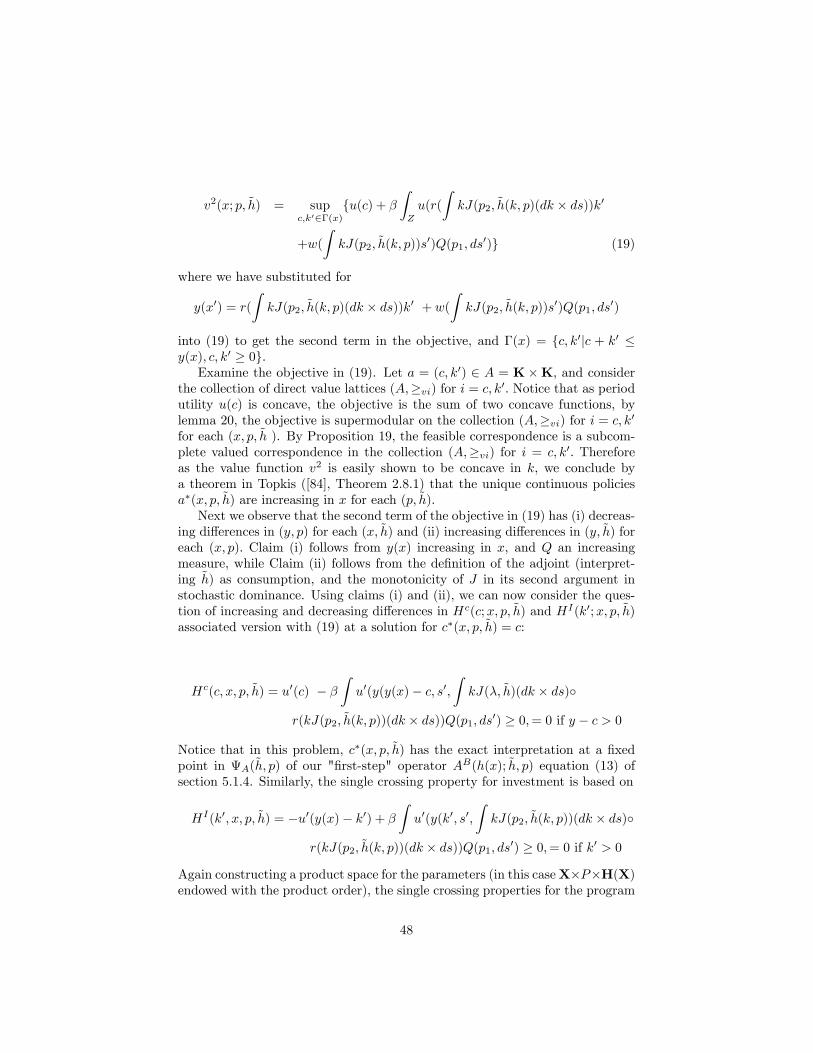
v2(x; p; ~h) = supc;k02�(x)

fu(c) + �ZZ

u(r(

ZkJ(p2; ~h(k; p)(dk � ds))k0

+w(

ZkJ(p2; ~h(k; p))s

0)Q(p1; ds0)g (19)

where we have substituted for

y(x0) = r(

ZkJ(p2; ~h(k; p)(dk � ds))k0 + w(

ZkJ(p2; ~h(k; p))s

0)Q(p1; ds0)

into (19) to get the second term in the objective, and �(x) = fc; k0jc + k0 �y(x); c; k0 � 0g:Examine the objective in (19). Let a = (c; k0) 2 A = K�K; and consider

the collection of direct value lattices (A;�vi) for i = c; k0: Notice that as periodutility u(c) is concave, the objective is the sum of two concave functions, bylemma 20, the objective is supermodular on the collection (A;�vi) for i = c; k0for each (x; p; ~h ). By Proposition 19, the feasible correspondence is a subcom-plete valued correspondence in the collection (A;�vi) for i = c; k0: Thereforeas the value function v2 is easily shown to be concave in k; we conclude bya theorem in Topkis ([84], Theorem 2.8.1) that the unique continuous policiesa�(x; p; ~h) are increasing in x for each (p; ~h):Next we observe that the second term of the objective in (19) has (i) decreas-

ing di¤erences in (y; p) for each (x; ~h) and (ii) increasing di¤erences in (y; ~h) foreach (x; p): Claim (i) follows from y(x) increasing in x, and Q an increasingmeasure, while Claim (ii) follows from the de�nition of the adjoint (interpret-ing ~h) as consumption, and the monotonicity of J in its second argument instochastic dominance. Using claims (i) and (ii), we can now consider the ques-tion of increasing and decreasing di¤erences in Hc(c;x; p; ~h) and HI(k0;x; p; ~h)associated version with (19) at a solution for c�(x; p; ~h) = c:

Hc(c; x; p; ~h) = u0(c) � �Zu0(y(y(x)� c; s0;

ZkJ(�; ~h)(dk � ds)�

r(kJ(p2; ~h(k; p))(dk � ds))Q(p1; ds0) � 0;= 0 if y � c > 0

Notice that in this problem, c�(x; p; ~h) has the exact interpretation at a �xedpoint in A(~h; p) of our "�rst-step" operator AB(h(x); ~h; p) equation (13) ofsection 5.1.4. Similarly, the single crossing property for investment is based on

HI(k0; x; p; ~h) = �u0(y(x)� k0) + �Zu0(y(k0; s0;

ZkJ(p2; ~h(k; p))(dk � ds)�

r(kJ(p2; ~h(k; p))(dk � ds))Q(p1; ds0) � 0;= 0 if k0 > 0

Again constructing a product space for the parameters (in this caseX�P�H(X)endowed with the product order), the single crossing properties for the program

48

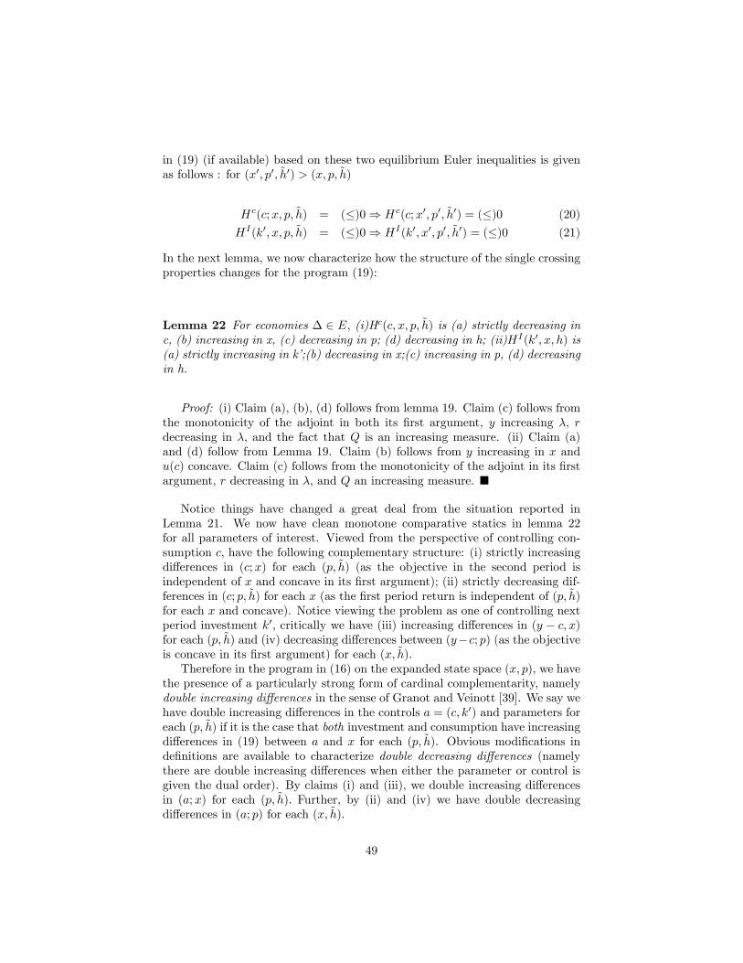
in (19) (if available) based on these two equilibrium Euler inequalities is givenas follows : for (x0; p0; ~h0) > (x; p; ~h)

Hc(c;x; p; ~h) = (�)0) Hc(c;x0; p0; ~h0) = (�)0 (20)

HI(k0; x; p; ~h) = (�)0) HI(k0; x0; p0; ~h0) = (�)0 (21)

In the next lemma, we now characterize how the structure of the single crossingproperties changes for the program (19):

Lemma 22 For economies � 2 E; (i)Hc(c; x; p; ~h) is (a) strictly decreasing inc, (b) increasing in x, (c) decreasing in p; (d) decreasing in h; (ii)HI(k0; x; h) is(a) strictly increasing in k�;(b) decreasing in x;(c) increasing in p, (d) decreasingin h.

Proof: (i) Claim (a), (b), (d) follows from lemma 19. Claim (c) follows fromthe monotonicity of the adjoint in both its �rst argument, y increasing �; rdecreasing in �; and the fact that Q is an increasing measure. (ii) Claim (a)and (d) follow from Lemma 19. Claim (b) follows from y increasing in x andu(c) concave. Claim (c) follows from the monotonicity of the adjoint in its �rstargument, r decreasing in �; and Q an increasing measure. �

Notice things have changed a great deal from the situation reported inLemma 21. We now have clean monotone comparative statics in lemma 22for all parameters of interest. Viewed from the perspective of controlling con-sumption c; have the following complementary structure: (i) strictly increasingdi¤erences in (c;x) for each (p; ~h) (as the objective in the second period isindependent of x and concave in its �rst argument); (ii) strictly decreasing dif-ferences in (c; p; ~h) for each x (as the �rst period return is independent of (p; ~h)for each x and concave). Notice viewing the problem as one of controlling nextperiod investment k0; critically we have (iii) increasing di¤erences in (y � c; x)for each (p; ~h) and (iv) decreasing di¤erences between (y�c; p) (as the objectiveis concave in its �rst argument) for each (x; ~h).Therefore in the program in (16) on the expanded state space (x; p), we have

the presence of a particularly strong form of cardinal complementarity, namelydouble increasing di¤erences in the sense of Granot and Veinott [39]. We say wehave double increasing di¤erences in the controls a = (c; k0) and parameters foreach (p; ~h) if it is the case that both investment and consumption have increasingdi¤erences in (19) between a and x for each (p; ~h). Obvious modi�cations inde�nitions are available to characterize double decreasing di¤erences (namelythere are double increasing di¤erences when either the parameter or control isgiven the dual order). By claims (i) and (iii), we double increasing di¤erencesin (a;x) for each (p; ~h): Further, by (ii) and (iv) we have double decreasingdi¤erences in (a; p) for each (x; ~h).

49

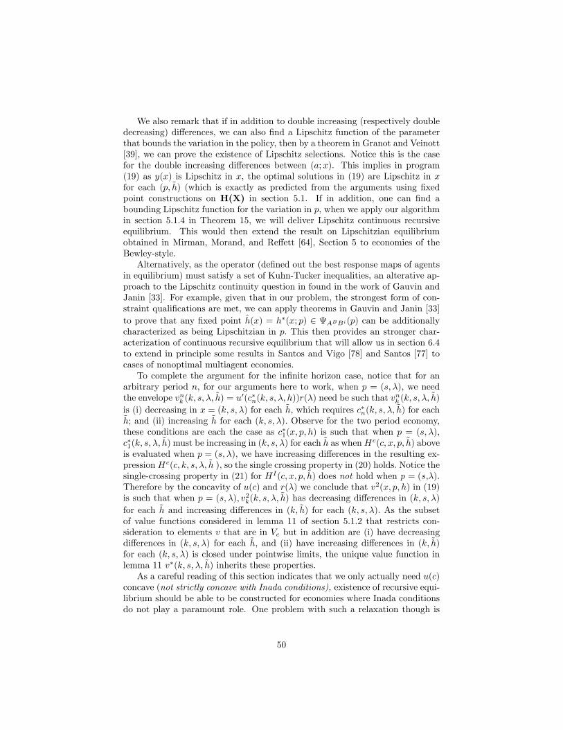
We also remark that if in addition to double increasing (respectively doubledecreasing) di¤erences, we can also �nd a Lipschitz function of the parameterthat bounds the variation in the policy, then by a theorem in Granot and Veinott[39], we can prove the existence of Lipschitz selections. Notice this is the casefor the double increasing di¤erences between (a;x). This implies in program(19) as y(x) is Lipschitz in x, the optimal solutions in (19) are Lipschitz in xfor each (p; ~h) (which is exactly as predicted from the arguments using �xedpoint constructions on H(X) in section 5.1. If in addition, one can �nd abounding Lipschitz function for the variation in p, when we apply our algorithmin section 5.1.4 in Theorem 15, we will deliver Lipschitz continuous recursiveequilibrium. This would then extend the result on Lipschitzian equilibriumobtained in Mirman, Morand, and Re¤ett [64], Section 5 to economies of theBewley-style.Alternatively, as the operator (de�ned out the best response maps of agents

in equilibrium) must satisfy a set of Kuhn-Tucker inequalities, an alterative ap-proach to the Lipschitz continuity question in found in the work of Gauvin andJanin [33]. For example, given that in our problem, the strongest form of con-straint quali�cations are met, we can apply theorems in Gauvin and Janin [33]to prove that any �xed point h(x) = h�(x; p) 2 ABBi(p) can be additionallycharacterized as being Lipschitzian in p: This then provides an stronger char-acterization of continuous recursive equilibrium that will allow us in section 6.4to extend in principle some results in Santos and Vigo [78] and Santos [77] tocases of nonoptimal multiagent economies.To complete the argument for the in�nite horizon case, notice that for an

arbitrary period n, for our arguments here to work, when p = (s; �); we needthe envelope vnk (k; s; �; ~h) = u

0(c�n(k; s; �; h))r(�) need be such that vnk (k; s; �;

~h)

is (i) decreasing in x = (k; s; �) for each ~h; which requires c�n(k; s; �; ~h) for each~h; and (ii) increasing ~h for each (k; s; �): Observe for the two period economy,these conditions are each the case as c�1(x; p; h) is such that when p = (s; �);c�1(k; s; �;

~h) must be increasing in (k; s; �) for each ~h as whenHc(c; x; p; ~h) aboveis evaluated when p = (s; �); we have increasing di¤erences in the resulting ex-pressionHc(c; k; s; �; ~h ), so the single crossing property in (20) holds. Notice thesingle-crossing property in (21) for HI(c; x; p; ~h) does not hold when p = (s;�):Therefore by the concavity of u(c) and r(�) we conclude that v2(x; p; h) in (19)is such that when p = (s; �); v2k(k; s; �; ~h) has decreasing di¤erences in (k; s; �)for each ~h and increasing di¤erences in (k; ~h) for each (k; s; �): As the subsetof value functions considered in lemma 11 of section 5.1.2 that restricts con-sideration to elements v that are in Vc but in addition are (i) have decreasingdi¤erences in (k; s; �) for each ~h; and (ii) have increasing di¤erences in (k; ~h)for each (k; s; �) is closed under pointwise limits, the unique value function inlemma 11 v�(k; s; �; ~h) inherits these properties.As a careful reading of this section indicates that we only actually need u(c)

concave (not strictly concave with Inada conditions), existence of recursive equi-librium should be able to be constructed for economies where Inada conditionsdo not play a paramount role. One problem with such a relaxation though is

50

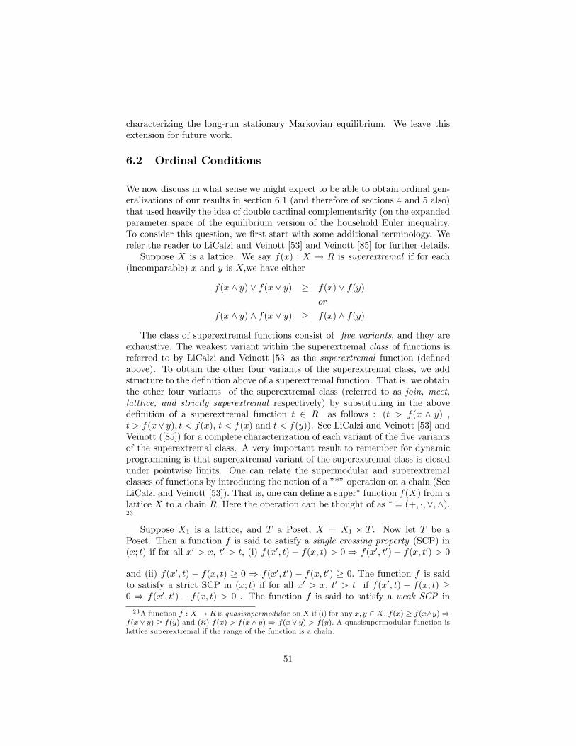
characterizing the long-run stationary Markovian equilibrium. We leave thisextension for future work.

6.2 Ordinal Conditions

We now discuss in what sense we might expect to be able to obtain ordinal gen-eralizations of our results in section 6.1 (and therefore of sections 4 and 5 also)that used heavily the idea of double cardinal complementarity (on the expandedparameter space of the equilibrium version of the household Euler inequality.To consider this question, we �rst start with some additional terminology. Werefer the reader to LiCalzi and Veinott [53] and Veinott [85] for further details.Suppose X is a lattice. We say f(x) : X ! R is superextremal if for each

(incomparable) x and y is X;we have either

f(x ^ y) _ f(x _ y) � f(x) _ f(y)or

f(x ^ y) ^ f(x _ y) � f(x) ^ f(y)

The class of superextremal functions consist of �ve variants, and they areexhaustive. The weakest variant within the superextremal class of functions isreferred to by LiCalzi and Veinott [53] as the superextremal function (de�nedabove). To obtain the other four variants of the superextremal class, we addstructure to the de�nition above of a superextremal function. That is, we obtainthe other four variants of the superextremal class (referred to as join, meet,latttice, and strictly superextremal respectively) by substituting in the abovede�nition of a superextremal function t 2 R as follows : (t > f(x ^ y) ,t > f(x_ y); t < f(x); t < f(x) and t < f(y)). See LiCalzi and Veinott [53] andVeinott ([85]) for a complete characterization of each variant of the �ve variantsof the superextremal class. A very important result to remember for dynamicprogramming is that superextremal variant of the superextremal class is closedunder pointwise limits. One can relate the supermodular and superextremalclasses of functions by introducing the notion of a �*�operation on a chain (SeeLiCalzi and Veinott [53]). That is, one can de�ne a super� function f(X) from alattice X to a chain R: Here the operation can be thought of as � = (+; �;_;^):23

Suppose X1 is a lattice, and T a Poset, X = X1 � T . Now let T be aPoset. Then a function f is said to satisfy a single crossing property (SCP) in(x; t) if for all x0 > x; t0 > t; (i) f(x0; t) � f(x; t) > 0 ) f(x0; t0) � f(x; t0) > 0

and (ii) f(x0; t) � f(x; t) � 0 ) f(x0; t0) � f(x; t0) � 0: The function f is saidto satisfy a strict SCP in (x; t) if for all x0 > x; t0 > t if f(x0; t) � f(x; t) �0 ) f(x0; t0) � f(x; t) > 0 . The function f is said to satisfy a weak SCP in

23A function f : X ! R is quasisupermodular on X if (i) for any x; y 2 X, f(x) � f(x^y))f(x_ y) � f(y) and (ii) f(x) > f(x^ y)) f(x_ y) > f(y): A quasisupermodular function islattice superextremal if the range of the function is a chain.

51

(x; t) if for all x0 > x; t0 > t if f(x0; t) � f(x; t) > 0 ) f(x0; t0) � f(x; t) � 0. As each superextremal variant in the superextremal class has an equivalentrepresentation using upcrossing di¤erences, one can view quasisupermodularfunctions with SCPs as variants of the superextremal class of functions (whenthe class is restricted to behavior along complementary chains). Let x; y 2 X,X a lattice. Then for our work, a complementary chain C(x; y) in X is theinterval [x ^ y; x _ y]: Then the upcrossing di¤erences for a mapping f(x) dis-cussed in LiCalzi and Veinott [53] within the superextremal class implies singlecrossing property representations in Milgrom and Shannon [62], and upcrossingdi¤erences must hold along C(x; y) for all x; y 2 X: We note that as men-tioned in section 6.1, a supermodular function will have upcrossing di¤erencesor equivalently increasing di¤erences on C(x; y): In this sense, quasisupermod-ular function provides an alternative characterization of many of the variants ofthe superextremal class, but also allow one to use superextremal methods whenthe underlying parameter space is merely a Poset.We now report a result in LiCalzi and Veinott ([53]) without proof. The

result provides a complete characterization of two variants of a superextremalfunction U(a) on a lattice A that we will consider for this discussion. We willthen remark how to extend our discussion to the other three superextremalvariants: Let (A;�) be a lattice. We have following characterizations of thesuperextremal variant of the superextremal class, and the lattice superextremalvariant:

Proposition 23 LiCalzi and Veinott ([53], Theorems1-3) Let (A,�) be a lat-tice, U(a) an extended real-valued mapping, a, �2 A. Then (a) U(a) is super-extremal i¤ either (i) U(a^a0) = U(a) ) U(a0) � U(a _ a0) or (ii) U(a_a0) =U(a) ) U(a ^ a0) � U(a0); (b)U(a) is lattice superextremal i¤ U(a) is super-extremal and U(a^a0) = u(a) ) U(a0) � U(a _ a0) and U(a_a0) = U(a) )U(a ^ a0) � u(a0):

A useful alternative characterization of (ii) is given in LiCalzi and Veinott[53]:

U(a) is lattice superextremal i¤ it is both join and meet superextremal:

i:e; U(a ^ a0) < (�)u(a)) U(a0) < (�)U(a _ a0)

One very useful property of the superextremal variant of the superextremal classof functions is that it is the only variant that is closed under pointwise limits.(See LiCalzi and Veinott [53], corollary 7).We now reconsider extensions of the decision-theoretic interpretation of the

methods for economies � 2 E for economies with ordinal forms of comple-mentarity. Again, in doing so, as in section 6.1, we are indicating where ourmonotonicity constructions within the two step procedure can be generalizedto settings without strong boundary conditions. The purpose of our discussionis to discuss exactly what sorts of ordinal extensions of our results might be

52

possible. Again begin by considering a two period economy where the economystarts the trivial distribution �0 that is associated with the situation where allagents are ex ante identical and have initial capital stock k0 > 0; and each facean initial state si0 = s0 that is �xed. Consider the decision problem in (19)for economies � 2 E0 initially: Therefore from the discussion in Section 6.1, ifagents are assumed to be given h 2 H(X); and (k0; s0; �0); we can then producea value function for the household as in (19) as the solution to the following twoperiod optimization problem (taking v0(x; h) = 0):

v2(x; p; ~h) = supc;k02�(x)

fu(c) + �ZZ

u(r(

ZkJ(p2; ~h(k; p)(dk � ds))k0

+w(

ZkJ(p2; ~h(k; p)))Q(p1; ds

0)g (22)

To see how we could relax the cardinal complementarities that were appliedin (19), �rst notice that as we assume the expected utility hypothesis, it willbe di¢ cult to relax any of the complementarity conditions between k0 and (p; ~h) to be weaker than cardinal as they are implicit in the second term of theobjective under the integral, and ordinal conditions are not additive. Further,as we need y(x) weakly increasing in x to obtain a strong set order comparisonfor the feasible correspondence �(x); this condition cannot be relaxed at thispoint either. Therefore to introduce ordinal versions of the cardinal comple-mentarities in (19), we focus on weakening the conditions that characterize thecomplementarities among the controls.At this stage therefore, the problem is very similar to the ordinal conditions

obtained in Mirman, Morand, and Re¤ett ([64], section 6.2). With Inada con-ditions on u(c); one can �rst observe by lemma 20 and using the de�nition ofthe meet and join on (A;�vc); for the objective on the right side of (22) tosuperextremal in any variant of the superextremal class on the consumptionvalue lattice (A;�vc); it is necessary for the second term in the objective to beconcave in k0: That is using the de�nition of meet at join on the consumptionvalue lattice, because of the Inada condition on c, we arrive at for any c > 0;when k01 < k

0

2 the need to check the condition

�

Zu0(y(k01; s

0;

ZkJ(�; ~h)(dk � ds) � r(kJ(p2; ~h(k; p))(dk � ds))Q(p1; ds0)

( � ) > u0(c)) (23)

�

Zu0(k02; s

0;

ZkJ(�; ~h)(dk � ds) � r(kJ(p2; ~h(k; p))(dk � ds))Q(p1; ds0)

( � ) > u0(c)

This echoes the result in Mirman, Morand, and Re¤ett ([64], Section 6.2) forthe homogeneous agent case. Interesting though, as y(0; s; �)>0, we can stillhave a lattice superextremal case that is not necessarily supermodular as in

53

Lemma 20: i.e., we just need for some c � 0; k0L > 0;

u0(c) > �

Zu0(y(k0L; s

0;

ZkJ(�; ~h)(dk�ds)�r(kJ(p2; ~h(k; p))(dk�ds))Q(p1; ds0)

(24)In this case, one does not need u(c) concave to obtain our complementarities inthe objective between (c; k0) described in section 6.2 on the investment lattice(A;�vk0): This remains true even if u(c) possesses an Inada condition, and thisis exactly di¤erent from the result for the homogeneous agent case in Mirman,Morand, and Re¤ett ([64], Section 6.2) because of the presence of uninsuredidiosyncratic labor income. Notice that once we obtain a "crossing", i.e, a pair(c�; k0�) such that

u0(c�) = �

Zu0(y(k0

�; s0;

ZkJ(�; ~h)(dk�ds)�r(kJ(p2; ~h(k; p))(dk�ds))Q(p1; ds0)

(25)at this stage u(c)must be concave. Now, the types of weakening of cardinal com-plementarities between a = (c; k0) on the lattice (A;�vk0) even when u(c) hasan Inada condition are allowed can then coincide with the various de�nitions ofsuperextremal complementarity given in Proposition 23. One should rememberthough that for forms of ordinal complementarities weaker than lattice super-extremal (e.g, superextremal, join-superextremal, meet-superextremal), by thekey characterization theorems in Li Calzi and Veinott ([53], Theorems 1-3), onewill not have sublatticed valued best responses in the program (19). In sucha case (remembering that the programming problem under consideration is nolonger associated with a strictly concave value function v2(k; s; �; ~h) in k (sobest responses are no longer single valued continuous maps, but rather uppersemi continuous correspondences), by the selection theorems on Veinott [85],Theorem 13 and 14) and the results in Smithson ([80]), we will only have aguarantee of a monotone selection. Although for applications of Tarski�s theo-rem in the �rst stage this is not in theory a problem, it becomes a much moredi¢ cult question to obtain a version of theorem 6 for such an economy.The rest of this section to be completed.

6.3 Monotone Comparative Dynamics on the Space ofEconomies

To be completed.

6.4 Lipschitzian Recursive Equilibrium and Numerical Ap-proximation

To be completed.

54

References

[1] Abian, S. and A.B. Brown. 1962. A theorem on partially order sets withapplications to �xed point theorems. Canadian Journal of Mathematics,13,78-82.

[2] Aliprantis, C. and K. Border. 1999. In�nite Dimensional Analysis, 2ndEdition. Springer.

[3] Amann, H. 1976. Fixed equations and nonlinear eigenvalue problems inordered Banach spaces. SIAM Review, 18(4), 620-709.

[4] Amir, R. L. Mirman, and W. Perkins. 1991, One-sector nonclassical optimalgrowth: optimality conditions and comparative dynamics. InternationalEconomic Review, 32, 625-644.

[5] Antoniadou, E. 1996. Lattice Programming and Economic Optimization.Ph.D. Dissertation. Stanford University

[6] Aiyagari, R. 1994. Uninsured idiosyncratic risk and aggregate saving. Quar-terly Journal of Economics, 109, 659-684.

[7] Aiyagari. R. 1995. Optimal capital income taxation with incomplete mar-kets, borrowing constraints, and constant discounting. Journal of PoliticalEconomy, 103( 6), 1158-1175.

[8] Becker R, and I. Zilcha. 1997. Stationary Ramsey equilibria under uncer-tainty. Journal of Economic Theory, 75, 122-140.

[9] Berge, C. 1963. Topological Spaces, reprint, Dover Press.

[10] Bergin, J. and D. Bernhardt. 1992. Anonymous sequential game with ag-gregate uncertainty. Journal of Mathematical Economics, 21, 543-562

[11] Bergin, J. and D. Bernhardt. 1995. Anonymous sequential games: existenceand characterization of equilibria. Economic Theory, 5, 461-489.

[12] Bewley, T. 1986. Stationary monetary equilibrium with a continuum of�uctuating consumers. in W. Hildenbrand and A. MasColell, ed., Contribu-tions in Mathematical Economics in honor of Gerald Debreu, Amsterdam,North-Holland.

[13] Bhattacharya, R. and Lee. 1988. Asymptotics of a class of Markov processesthat are not in general irreducible. Annals of Probability, 16, 1333-1347.

[14] Birkho¤, G. 1967. Lattice Theory, 3rd Edition. AMS Press.

[15] Bizer, D. and K. Judd. 1989. Taxation and uncertainty. American EconomicReview, 79, 331-336.

[16] Brock, W. and L. Mirman. 1972. Optimal growth and uncertainty: thediscounted case. Journal of Economic Theory, 4, 479-513

55

[17] Clarke, F. 1983. Optimization and Nonsmooth Analysis. SIAM Press.

[18] Coleman, W.J. II. 1990. Solving the stochastic growth model by policy-function iteration. Journal of Business and Economic Statistics, 8, 27-29.

[19] Coleman, W.J., II. 1991. Equilibrium in a production economy with anincome tax. Econometrica, 59, 1091-1104.

[20] Coleman, W.J., II. 1997. Equilibria in distorted in�nite-horizon economieswith capital and labor, Journal of Economic Theory 72 (1997) , 446-461.

[21] Coleman, W. J., II. 2000. Uniqueness of an equilibrium in in�nite-horizoneconomies subject to taxes and externalities , Journal of Economic Theory95 (2000), 71-78.

[22] Dacic, R. 1979. Fixed points of antitone mappings in condiional completepartially ordered sets. Publications de L�Insititut Mathématique, 83-90.

[23] Dacic, R. 1983. On �xed edges of antitone self-mappings of complete lat-tices. Publications de L�Insititut Mathématique, 49-53.

[24] Denardo, E. 1967. Contraction mappings in the theory underlying dynamicprogramming. SIAM Review, 9, 165-177.

[25] Datta, M., Mirman, L., and K. Re¤ett. 2002. Existence and uniqueness ofequilibrium in distorted dynamic economies with capital and labor Journalof Economic Theory, 103, 377-410

[26] Datta, M., Mirman, L, Morand, O., and K. Re¤ett. 2002. Monotone meth-ods for Markovian equilibrium in dynamic economies. Annals of OperationsResearch, 114, 117-144

[27] Datta, M., L. Mirman, O. Morand, and K. Re¤ett. 2002. Markovian Equi-librium in In�nite Horizon Models with Many Agents, Incomplete Markets,and Public Policy, MS. Arizona State University.

[28] Dieudonne, J. 1960. Foundations of Modern Analysis, Academic Press.

[29] Du¢ e, D. J. Geanokopolis, A. MasColell, and A. McClennen. 1994. Sta-tionary Markov Equilibriua. Econometrica, 62, 745-781.

[30] Dugundji, J and A. Granas. 1982. Fixed Point Theory. Warsaw Scienti�cPress.

[31] Echenique, F. 2003. A short and constructive proof of Tarski�s �xed pointtheorem. MS, Cal Tech.

[32] Erikson, J. 2003. An order theoretic approach to Markovian Equilibriumin overlapping generations economies with stochastic Production. MS. Ari-zona State University.

56

[33] Gauvin, J. and R. Janin. 1988. Directional behavior of optimal solutionsin nonlinear mathematical programming. Mathematics of Operations Re-search, 13(4), 629-649.

[34] Granas, A. and J. Dugundji. 2003. Fixed Point Theory, Springer Press.

[35] Greenwood, J., and G. Hu¤man. 1995. On the existence of nonoptimalequilibria in dynamic stochastic economies, Journal of Economic Theory,65, 611-623.

[36] Guillerme, J. 1995. Intermediate value theoerems and �xed point theoremsfor semi-continuous functions on product spaces. Proceedings of the Amer-ican Mathematical Society, 123(7), 2119-2122.

[37] Feldman, M. and C. Gilles. 1985.An expository note on individual riskwithout aggregate uncertainty. Journal of Economic Theory, 35, 26-32.

[38] Futia, C. 1982. Invariant distributions and the limiting behavior of Markov-ian economic models. Econometrica, 50, 377-408.

[39] Granot, F and A.Veinott, Jr. 1985. Substitutes, complements, and ripplesin network �ows. Mathematics of Operations Research, 471-497.

[40] Hopenhayn, H. and E. Prescott. 1987. Invariant distributions for monotoneMarkov processes. MS. University of Minnesota.

[41] Hopenhayn, H.. and E. Prescott. 1992. Stochastic monotonicity and station-ary distributions for dynamic economies. Econometrica, 60(6), 1387-1406.

[42] Huggett, M. 1997. The one-sector growth model with idiosyncratic shocks.Journal of Monetary Economics. 39, 385-403

[43] Huggett, M. 2003. When are comparative dynamics monotone. Review ofEconomics Dynamics, 6, 1-11.

[44] Hutson, V, and J. Pym. 1980. Applications of Functional Analysis andOperator Theory, Academic Press.

[45] Judd, K. 1998. Numerical Methods in Economics. MIT Press.

[46] Krasnoselskii, M. 1964. Positive solutions of Operator Equations. Noordho¤Press.

[47] Kehoe, T., D. Levine, and P. Romer. 1992. On characterizing equilibria ofeconomies with externalities and taxes as solutions to optimization prob-lems. Economic Theory, 2, 43-68.

[48] Krebs, T. 2002. Non-Existence of Recursive Equilibria on Compact StateSpaces When Markets Are Incomplete. forthcoming in Journal of EconomicTheory.

57

[49] Krebs, T. 2002. Recursive equilibrium in endogeneous growth models withincomplete markets. MS. Brown University.

[50] Krusell, P. and A. Smith. 1998. Income and wealh heterogeneity in a macro-economy. Journal of Political Economy, 105, 867-896.

[51] Kubler, F. and K. Schmedders. 2002. Recursive equilibrium in economieswith incomplete markets. Macroeconomic Dynamics, 6, 284-306.

[52] Jovanovic, B. and R. Rosenthal. 1988. Anonymous sequential games. Jour-nal of Mathematical Economics, 17, 77-87.

[53] Li Calzi, M. and A. Veinott, Jr. 1991. Subextremal functions and latticeprogramming. MS. Stanford University.

[54] LeVan, C. and L. Morhaim. 2002. Optimal growth models with boundedand unbounded returns: a unifying approach. Journal of Economic Theory,105, 158-187.

[55] LeVan, C. and Y. Vailakis. 2003. Existence of a competitive equilibriumin a one sector growth model with heterogeneous agents and irreversibleinvestment. forthcoming Economic Theory.

[56] Ljungqvist, L. and T. Sargent. 2000. Recursive Macroeconomy Theory. MITPress.

[57] Lucas, R.E., Jr. 1980. Equilibrium in a Pure Currency Economy. EconomicInquiry, 18, 203-220.

[58] Lucas, R.E., Jr. and N. Stokey. Money and interest in a cash-in-advanceeconomy. Econometrica, 55, 1821-37.

[59] Lucas, R.E., Jr. and E. Prescott. 1971. Investment under uncertainty.Econometica, 39, 659-681.

[60] Miao, J. 2002. Stationary equilibria of economies with a continuum of het-erogeneous consumers. MS. University of Rochester.

[61] Miao, J. 2003. Competitive equilibria in economies with a continuum ofconsumer and aggregate shocks. MS. University of Rochester.

[62] Milgrom, P. and C. Shannon. 1994. Monotone comparative statics. Econo-metrica, 62, 157-180.

[63] Mirman, L. J., and I. Zilcha. 1975. On optimal growth under uncertainty.Journal of Economic Theory, 11, 329-339.

[64] Mirman, L.J, O. Morand, and K. Re¤ett. 2003. A qualitative approachto Markovian equilibrium in in�nite horizon economies with capital. MS.Arizona State University.

58

[65] Moore, R.E. 1966. Inteval Analysis. Prentice Hall.

[66] Moore, R.E. 1978. Bounding sets in function spcaes with applications tononlinear operator equations. SIAM Review, 20(3), 492-512.

[67] Moore, R.E. 1979. Methods and applications of interval analysis. SIAMStudies in Applied Mathmatics, vol 2.

[68] Morand, O. and K.L. Re¤ett. 2003. Existence and Uniqueness of Equilib-rium in Nonoptimal Unbounded In�nite Horizon Economies. forthcomingin Journal of Monetary Economics.

[69] Prescott, E. and R. Mehra. 1980. Recursive competitive equilibrium: thecase of homogeneous households. Econometrica, 1365-1379.

[70] Rall, L.B., 1982. A theory of interval iteration. Proceedings of the AmericanMathematical Society. 625-631.

[71] Re¤ett, K. 2003. Markovian Equilibrium with Dynamic Complementaritiesin Many Dimensions. MS. Arizona State University.

[72] Re¤ett, K. 2003. Concave-modular dynamic programming with applica-tions. MS. Arizona State University.

[73] Re¤ett, K. 2003. Computing economic theory: applications of monotoneiterative interval methods. MS. Arizona State University.

[74] Rockafellar, R.T. 1970. Convex Analysis. Princeton Press.

[75] Santos, M. 1991. Smoothness of the policy function in discrete-time models.Econometrica, 1365-1382.

[76] Santos, M. 2002. On non existence of Markov equilibria in competitive-market economies.�Journal of Economic Theory, 105, 73-98.

[77] Santos, Manuel. 2000. The numerical accuracy of numerical solutions usingEuler residuals. Econometrica, 68, 1377-140 :

[78] Santos, M. and J. Vigo-Aguiar. 1998. Analysis of a numerical dynamicprogramming algorithm applied to economic models. Econometrica, 66,409-426.

[79] Scarf, H. 1973. The Computation of Economic Equilibria (with T. Hansen).Yale Press: New Haven.

[80] Smithson, R. 1971. Fixed points of order preserving multifunctions. Pro-ceedings of the American Mathematical Society, 28(1), 304-310.

[81] Stachurski, J. 2002. Stochastic optimal growth with unbounded shocks.Journal of Economic Theory, 106, 45-60.

59

[82] Stokey, N., R.E. Lucas, Jr., with E. Prescott. 1989. Recursive methods ineconomic dynamics. Harvard Press

[83] Tarski, A. 1955. A lattice-theoretical �xpoint theorem and its applications.Paci�c Journal of Mathematics, 5, 285-309.

[84] Topkis, D. 1998. Supermodularity and Complementarity. Princeton Press.

[85] Veinott, A. 1992. Lattice programming: qualitative optimization and equi-libria. MS. Stanford.

[86] Zeidler, E. 1986. Nonlinear functional analysis and its applications: vol 1,Fixed Point Theory. Springer Press.

[87] Zhou, L. 1994. The set of Nash equilibria of a supermodular game is acomplete lattice. Games and Economic Behavior, 7, 295-300.

60