Chapter 2

Multirate digital signal processing

In multirate digital signal processing the sampling rate of a signal is changed in or-der to increase the efficiency of various signal processing operations. Decimation, ordown-sampling, reduces the sampling rate, whereas expansion, or up-sampling, fol-lowed by interpolation increases the sampling rate. Some applications of multiratesignal processing are:

• Up-sampling, i.e., increasing the sampling frequency, before D/A conversion inorder to relax the requirements of the analog lowpass antialiasing filter. Thistechnique is used in audio CD, where the sampling frequency 44.1 kHz is increasedfourfold to 176.4 kHz before D/A conversion.

• Various systems in digital audio signal processing often operate at different sam-pling rates. The connection of such systems requires a conversion of samplingrate.

• Decomposition of a signal into M components containing various frequency bands.If the original signal is sampled at the sampling frequency fs (with a frequencyband of width fs/2, or half the sampling frequency), every component then con-tains a frequency band of width 1

2fs/M only, and can be represented using the

sampling rate fs/M . This allows for efficient parallel signal processing with pro-cessors operating at lower sampling rates. The technique is also applied to datacompression in subband coding, for example in speech processing, where the vari-ous frequency band components are represented with different word lengths.

• In the implementation of high-performance filtering operations, where a very nar-row transition band is required. The requirement of narrow transition bands leadsto very high filter orders. However, by decomposing the signal into a number ofsubbands containing the passband, stopband and transition bands, each compo-nent can be processed at a lower rate, and the transition band will be less narrow.Hence the required filter complexity may be reduced significantly.

The theory of multirate signal processing is quite extensive, and not entirely trivial.Here we will discuss some of the main ideas only.

20

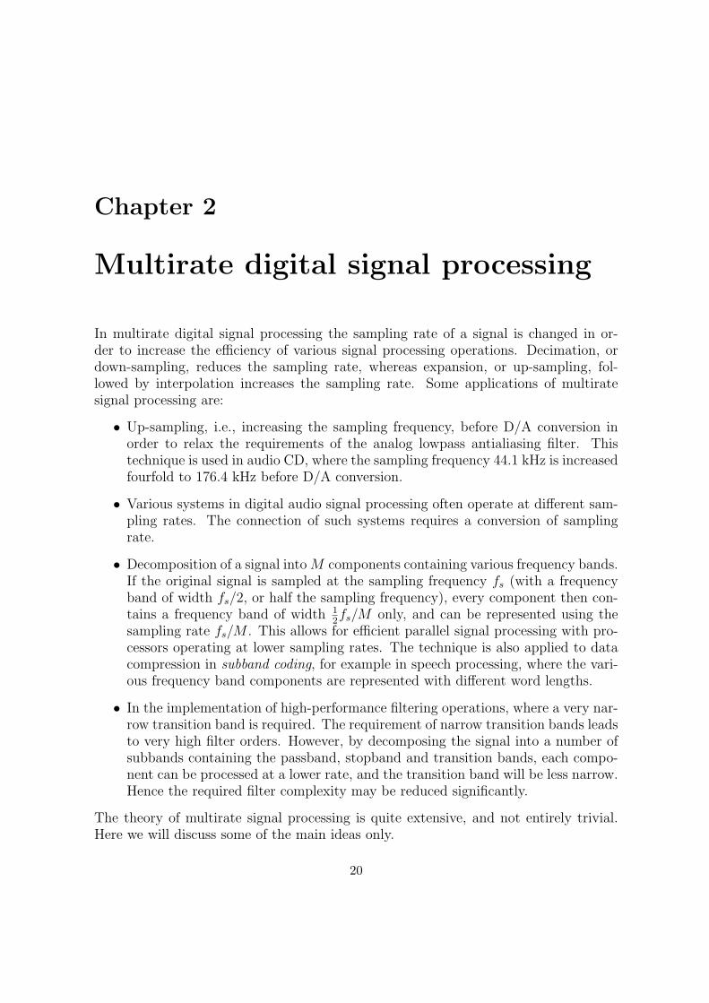
-- ↓ M y(m)x(n)

Figure 2.1: Decimation by the factor M .

2.1 Basic operations of multirate processing

2.1.1 Sampling rate conversion

Decimation.Decimation, or down-sampling, consists of reducing the sampling rate by a factor M ,cf. Figure 2.1. Here, the output is defined as

y(m) = x(mM) (2.1)

i.e., it consists of every Mth element of the input signal. It is clear that the decimatedsignal y does not in general contain all information about the original signal x. There-fore, decimation is usually applied in filter banks and preceded by filters which extractthe relevant frequency bands, cf. Figure 2.3.

In order to analyze the frequency domain characteristics of a multirate processingsystem with decimation, we need to study the relation between the Fourier transforms,or the z-transforms, of the signals x and y. For simplicity we consider the case M = 2only. Then the decimated signal y is given by

y(m) = x(2m) (2.2)

or {y(m)} = {x(0), x(2), x(4), . . .}. Given the z-transform of {x(n)},x(z) = x(0) + x(1)z−1 + x(2)z−2 + · · ·+ x(n)z−n + · · · (2.3)

we should like to have an expression for the z-transform of {y(m)}, i.e. (using (2.2)),

y(z) = y(0) + y(1)z−1 + y(2)z−2 + · · ·+ y(m)z−m + · · ·= x(0) + x(2)z−1 + x(4)z−2 + · · ·+ x(2m)z−m + · · · (2.4)

In order to derive an expression for the z-transform of y, it is convenient to representthe decimation in two stages as follows. First, define the signal

{v(n)} = {x(0), 0, x(2), 0, x(4), 0, . . .} (2.5)

which has the z-transform

v(z) = x(0) + x(2)z−2 + x(4)z−4 + · · ·+ x(2m)z−2m + · · · (2.6)

21

Asx(−z) = x(0)− x(1)z−1 + x(2)z−2 − · · ·+ x(2m)z−2m + · · · (2.7)

it follows that

v(z) =1

2

(x(z) + x(−z)

)(2.8)

By (2.4) and (2.6), y(z) = v(z1/2). Hence we have obtained the relation

y(z) =1

2

(x(z1/2) + x(−z1/2)

)(2.9)

In order to determine the frequency domain characteristics of the decimated signal{y(m)}, recall that the Fourier transform is related to the z-transform according to

Y (ω) = y(z)∣∣∣z=ejω

(2.10)

Hence, we have from (2.9),

Y (ω) =1

2

(x(ejω/2) + x(−ejω/2)

)(2.11)

Noting that −1 = ejπ, it follows that

Y (ω) =1

2

(x(ejω/2) + x(ej(ω/2+π))

)

=1

2

(X(ω/2) + X(ω/2 + π)

)(2.12)

where X is the Fourier-transform of the sequence {x(n)}. But from the propertiesof the Fourier transform (periodicity and symmetry) it follows that X(ω/2 + π) =X(ω/2− π) = X(π − ω/2)∗. Hence

Y (ω) =1

2

(X(ω/2) + X(π − ω/2)∗

)(2.13)

The Fourier-transform of {y(m)} thus cannot distinguish between the frequencies ω/2and π−ω/2 of {x(n)}. This is equivalent to the frequency folding phenomenon occur-ring when sampling a continuous-time signal.

Hence, whereas the signal {x(n)} consists of frequencies in [0, π], the frequencycontents of the decimated signal {y(m)} are restricted to the range [0, π/2]. Moreover,after decimation of the signal {x(n)}, its frequency components in [0, π/2] cannot bedistinguished from the frequency components in the range [π/2, π]

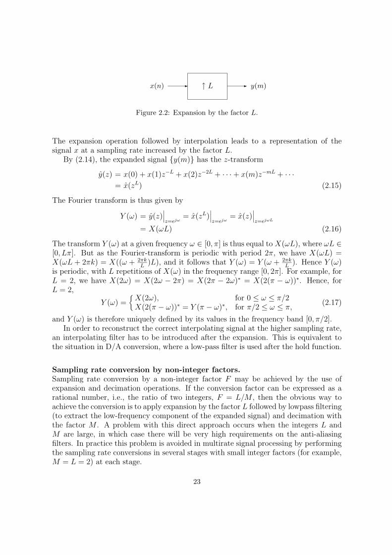
Expansion.Expansion, or up-sampling, consists of increasing the sampling rate by a factor L,cf. Figure 2.2. Here, the output is obtained by inserting L−1 zeros between successivevalues of the input x(n), i.e.

y(m) ={

x(m/L), for m = 0, L, 2L, . . .0, otherwise.

(2.14)

22

-- ↑ L y(m)x(n)

Figure 2.2: Expansion by the factor L.

The expansion operation followed by interpolation leads to a representation of thesignal x at a sampling rate increased by the factor L.

By (2.14), the expanded signal {y(m)} has the z-transform

y(z) = x(0) + x(1)z−L + x(2)z−2L + · · ·+ x(m)z−mL + · · ·= x(zL) (2.15)

The Fourier transform is thus given by

Y (ω) = y(z)∣∣∣z=ejω

= x(zL)∣∣∣z=ejω

= x(z)∣∣∣z=ejωL

= X(ωL) (2.16)

The transform Y (ω) at a given frequency ω ∈ [0, π] is thus equal to X(ωL), where ωL ∈[0, Lπ]. But as the Fourier-transform is periodic with period 2π, we have X(ωL) =X(ωL + 2πk) = X((ω + 2πk

L)L), and it follows that Y (ω) = Y (ω + 2πk

L). Hence Y (ω)

is periodic, with L repetitions of X(ω) in the frequency range [0, 2π]. For example, forL = 2, we have X(2ω) = X(2ω − 2π) = X(2π − 2ω)∗ = X(2(π − ω))∗. Hence, forL = 2,

Y (ω) ={

X(2ω), for 0 ≤ ω ≤ π/2X(2(π − ω))∗ = Y (π − ω)∗, for π/2 ≤ ω ≤ π,

(2.17)

and Y (ω) is therefore uniquely defined by its values in the frequency band [0, π/2].In order to reconstruct the correct interpolating signal at the higher sampling rate,

an interpolating filter has to be introduced after the expansion. This is equivalent tothe situation in D/A conversion, where a low-pass filter is used after the hold function.

Sampling rate conversion by non-integer factors.Sampling rate conversion by a non-integer factor F may be achieved by the use ofexpansion and decimation operations. If the conversion factor can be expressed as arational number, i.e., the ratio of two integers, F = L/M , then the obvious way toachieve the conversion is to apply expansion by the factor L followed by lowpass filtering(to extract the low-frequency component of the expanded signal) and decimation withthe factor M . A problem with this direct approach occurs when the integers L andM are large, in which case there will be very high requirements on the anti-aliasingfilters. In practice this problem is avoided in multirate signal processing by performingthe sampling rate conversions in several stages with small integer factors (for example,M = L = 2) at each stage.

23

An implementation of sampling rate conversion is given by the Matlab routiney = resample(x,L,M)

which resamples the sequence in vector x at L/M times the original sampling rate.Before resampling, an anti-aliasing (lowpass) FIR filter is applied to x.

Sampling rate conversion of a finite-length sequence.A sequence of finite length can be resampled in a very straightforward way as follows.Assume that the sequence

{x(n)} = {x(0), x(1), . . . , x(N − 1)}of length N has been obtained by sampling a continuous-time, analog, signal xa(t) withsampling frequency fx, so that

x(n) = xa(nTx)

where Tx = 1/fx is the associated sampling period.We want to determine another sequence

{y(m)} = {y(0), y(1), . . . , y(M − 1)}of length M > N corresponding to the sampling frequency fy = M

Nfx, so that

y(m) = xa(mTy)

where Ty = 1/fy is the associated sampling period. Notice that Ty = NM

Tx, so thatMTy = NTx and the sequences {x(n)} and {y(m)} cover the same continuous timeinterval.

The resampled sequence can be determined by observing that there is a simplerelationship between the Fourier transforms of the given sequence {x(n)} and theresampled sequence {y(m)}.

Let {x(n)} have Fourier transform {X(k)}. Assuming that the underlying analogsignal xa(t) is bandlimited, so that its Fourier transform Xa(ω) vanishes for ω ≥ πfx,i.e., there is no aliasing when xa(t) is sampled using sampling frequency fx, we have(see introductory course in signal processing)

X(k) =1

Tx

Xa(2πfxk/N), k = 0, 1, . . . , N/2

andX(N − k) = X(k)∗

where we have for convenience assumed that N is even. Similarly, for the Fouriertransform {Y (l)} of the resampled sequence {y(m)} we have

Y (l) =1

Ty

Xa(2πfyl/M), l = 0, 1, . . . , M/2

andY (M − l) = Y (l)∗

24

But fy = MN

fx implies fy/M = fx/N Hence the first N/2 elements of Y (l) are given by

Y (l) =1

Ty

Xa(2πfxl/N) =Tx

Ty

X(l)

=M

NX(l), l = 0, 1, . . . , N/2

As Xa(ω) vanishes for larger frequencies, the corresponding elements Y (l) are zero,

Y (l) = 0, k = N/2 + 1, . . . , M/2

Finally, by symmetricity of the Fourier transform we have

Y (M − l) = Y (l)∗

Having obtained its Fourier transform, the resampled sequence {y(m)} can be deter-mined by taking the inverse Fourier transform of {Y (l)}.

Notice that the above procedure requires only a standard Fourier transform ofthe given sequence followed by scaling, zero padding and inverse Fourier transform.Observe that if the intermediate Fourier transform operations are eliminated, the pro-cedure reduces to Shannon reconstruction, where the resampled sequence {y(m)} isexpressed explicitly in terms of the original sequence {x(n)}.

2.1.2 Analysis and synthesis filter banks

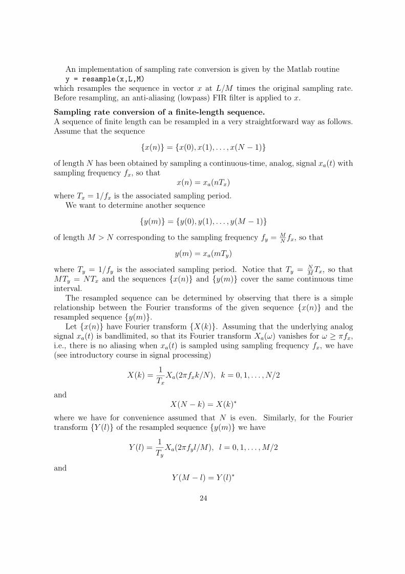
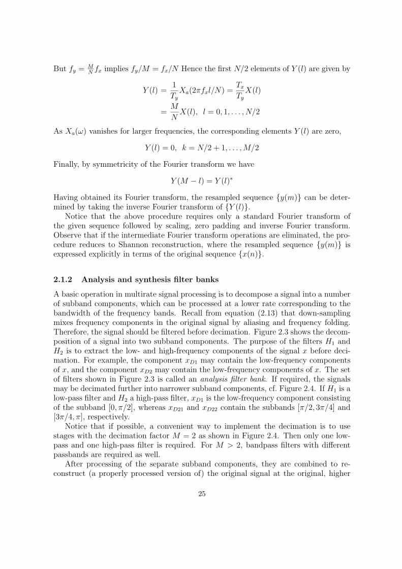
A basic operation in multirate signal processing is to decompose a signal into a numberof subband components, which can be processed at a lower rate corresponding to thebandwidth of the frequency bands. Recall from equation (2.13) that down-samplingmixes frequency components in the original signal by aliasing and frequency folding.Therefore, the signal should be filtered before decimation. Figure 2.3 shows the decom-position of a signal into two subband components. The purpose of the filters H1 andH2 is to extract the low- and high-frequency components of the signal x before deci-mation. For example, the component xD1 may contain the low-frequency componentsof x, and the component xD2 may contain the low-frequency components of x. The setof filters shown in Figure 2.3 is called an analysis filter bank. If required, the signalsmay be decimated further into narrower subband components, cf. Figure 2.4. If H1 is alow-pass filter and H2 a high-pass filter, xD1 is the low-frequency component consistingof the subband [0, π/2], whereas xD21 and xD22 contain the subbands [π/2, 3π/4] and[3π/4, π], respectively.

Notice that if possible, a convenient way to implement the decimation is to usestages with the decimation factor M = 2 as shown in Figure 2.4. Then only one low-pass and one high-pass filter is required. For M > 2, bandpass filters with differentpassbands are required as well.

After processing of the separate subband components, they are combined to re-construct (a properly processed version of) the original signal at the original, higher

25

H1(z)x ↓ 2- - -xD1

H2(z) -- ↓ 2 -xD2

Figure 2.3: Signal decomposition into subband components.

H1(z)

H1(z)

x ↓ 2

↓ 2

- -

-

-

-

xD1

H2(z)

H2(z)

-

-

-

-

↓ 2

↓ 2

-

-

xD2 xD21

xD22

Figure 2.4: Filter bank for signal decomposition.

26

Analysis filter bank Synthesis filter bank

H1(z)x ↓ 2- - - -xD1rrr ↑ 2 - G1(z)

xE1 -- y

H2(z) -- ↓ 2 - -xD2rrr ↑ 2 - G2(z)xE2

6g+

+

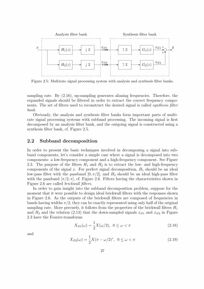
Figure 2.5: Multirate signal processing system with analysis and synthesis filter banks.

sampling rate. By (2.16), up-sampling generates aliasing frequencies. Therefore, theexpanded signals should be filtered in order to extract the correct frequency compo-nents. The set of filters used to reconstruct the desired signal is called synthesis filterbank.

Obviously, the analysis and synthesis filter banks form important parts of multi-rate signal processing systems with subband processing. The incoming signal is firstdecomposed by an analysis filter bank, and the outgoing signal is constructed using asynthesis filter bank, cf. Figure 2.5.

2.2 Subband decomposition

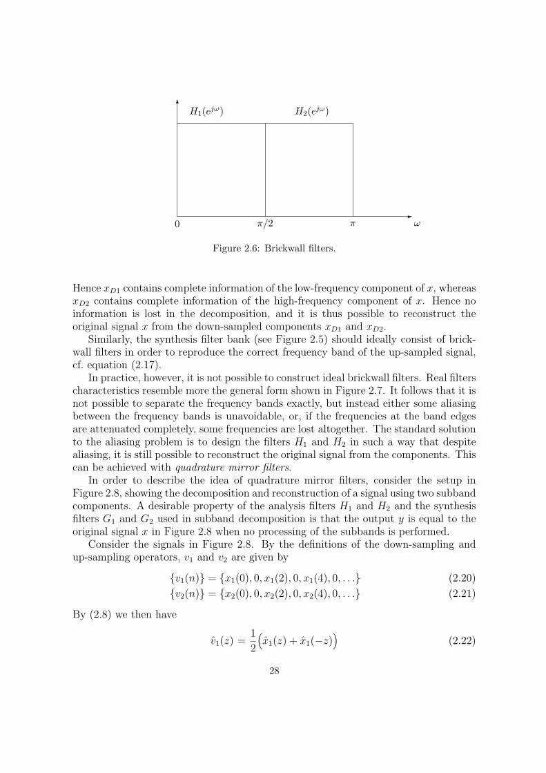
In order to present the basic techniques involved in decomposing a signal into sub-band components, let’s consider a simple case where a signal is decomposed into twocomponents: a low-frequency component and a high-frequency component. See Figure2.3. The purpose of the filters H1 and H2 is to extract the low- and high-frequencycomponents of the signal x. For perfect signal decomposition, H1 should be an ideallow-pass filter with the passband [0, π/2], and H2 should be an ideal high-pass filterwith the passband [π/2, π], cf. Figure 2.6. Filters having the characteristics shown inFigure 2.6 are called brickwall filters.

In order to gain insight into the subband decomposition problem, suppose for themoment that it were possible to design ideal brickwall filters with the responses shownin Figure 2.6. As the outputs of the brickwall filters are composed of frequencies inbands having widths π/2, they can be exactly represented using only half of the originalsampling rate. More precisely, it follows from the properties of the brickwall filters H1

and H2 and the relation (2.13) that the down-sampled signals xD1 and xD2 in Figure2.3 have the Fourier-transforms

XD1(ω) =1

2X(ω/2), 0 ≤ ω < π (2.18)

and

XD2(ω) =1

2X(π − ω/2)∗, 0 ≤ ω < π (2.19)

27

-

6

ωππ/20

H1(ejω) H2(ejω)

Figure 2.6: Brickwall filters.

Hence xD1 contains complete information of the low-frequency component of x, whereasxD2 contains complete information of the high-frequency component of x. Hence noinformation is lost in the decomposition, and it is thus possible to reconstruct theoriginal signal x from the down-sampled components xD1 and xD2.

Similarly, the synthesis filter bank (see Figure 2.5) should ideally consist of brick-wall filters in order to reproduce the correct frequency band of the up-sampled signal,cf. equation (2.17).

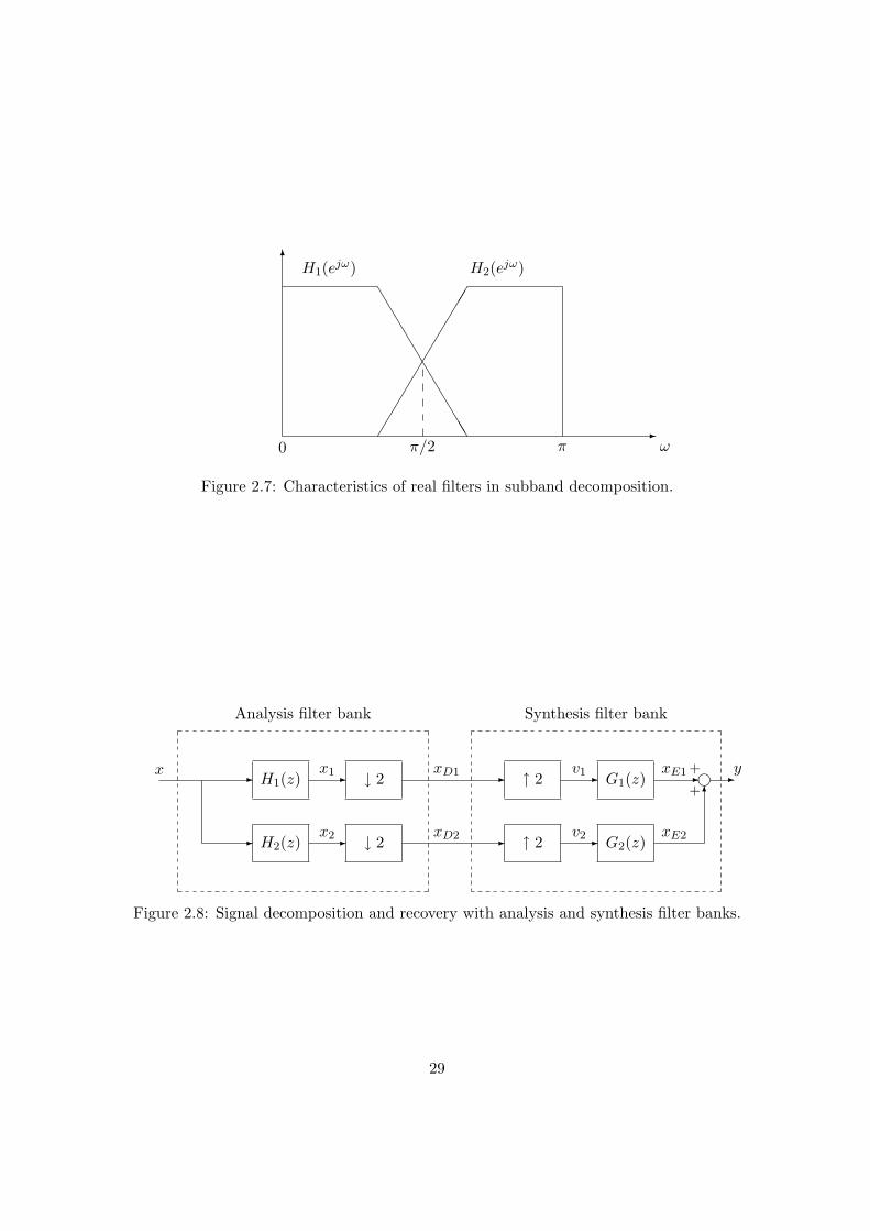
In practice, however, it is not possible to construct ideal brickwall filters. Real filterscharacteristics resemble more the general form shown in Figure 2.7. It follows that it isnot possible to separate the frequency bands exactly, but instead either some aliasingbetween the frequency bands is unavoidable, or, if the frequencies at the band edgesare attenuated completely, some frequencies are lost altogether. The standard solutionto the aliasing problem is to design the filters H1 and H2 in such a way that despitealiasing, it is still possible to reconstruct the original signal from the components. Thiscan be achieved with quadrature mirror filters.

In order to describe the idea of quadrature mirror filters, consider the setup inFigure 2.8, showing the decomposition and reconstruction of a signal using two subbandcomponents. A desirable property of the analysis filters H1 and H2 and the synthesisfilters G1 and G2 used in subband decomposition is that the output y is equal to theoriginal signal x in Figure 2.8 when no processing of the subbands is performed.

Consider the signals in Figure 2.8. By the definitions of the down-sampling andup-sampling operators, v1 and v2 are given by

{v1(n)} = {x1(0), 0, x1(2), 0, x1(4), 0, . . .} (2.20)

{v2(n)} = {x2(0), 0, x2(2), 0, x2(4), 0, . . .} (2.21)

By (2.8) we then have

v1(z) =1

2

(x1(z) + x1(−z)

)(2.22)

28

-

6

ωππ/20···········T

TTTTTTTTTT

H1(ejω) H2(ejω)

Figure 2.7: Characteristics of real filters in subband decomposition.

Analysis filter bank Synthesis filter bank

H1(z)x x1 ↓ 2- - -xD1 ↑ 2 -v1

G1(z)xE1 -- y

H2(z) -- x2 ↓ 2 -xD2 ↑ 2 -v2G2(z)

xE2

6g+

+

Figure 2.8: Signal decomposition and recovery with analysis and synthesis filter banks.

29

v2(z) =1

2

(x2(z) + x2(−z)

)(2.23)

or

v1(z) =1

2

(H1(z)x(z) + H1(−z)x(−z)

)(2.24)

v2(z) =1

2

(H2(z)x(z) + H2(−z)x(−z)

)(2.25)

The output is given by

y(z) = xE1(z) + xE2(z)

= G1(z)v1(z) + G2(z)v2(z) (2.26)

Combining (2.26) and (2.24), (2.25) gives

y(z) =1

2

(G1(z)H1(z) + G2(z)H2(z)

)x(z)

+1

2

(G1(z)H1(−z) + G2(z)H2(−z)

)x(−z) (2.27)

The first term in (2.27) is the desired output signal, whereas the second term representsthe spurious component caused by aliasing. Aliasing is avoided if we require that

G1(z)H1(−z) + G2(z)H2(−z) = 0 (2.28)

This can be achieved in a straightforward way by selecting G1(z) and G2(z) as

G1(z) = 2H2(−z) (2.29)

G2(z) = −2H1(−z) (2.30)

where the scaling factors 2 are introduced for convenience.Moreover, if the analysis filter H1(z) is a lowpass filter, then H2(z) is typically its

symmetric highpass filter, i.e., cf. equation (1.11),

H2(z) = H1(−z) (2.31)

Then (2.29) and (2.30) imply

G1(z) = 2H1(z) (2.32)

G2(z) = −2H2(z) (2.33)

Combining the expressions for G1 and G2 with the expression (2.27) for the systemoutput gives

y(z) =(H1(z)2 −H1(−z)2

)x(z) (2.34)

Equation (2.34) implies that there is no aliasing affecting the output, which is a verydesirable property indeed. The condition for exact signal recovery is

H1(z)2 −H1(−z)2 = Kz−P (2.35)

30

where K is a constant and P denotes a time delay which cannot be avoided when usingcausal filters.

The filters which satisfy the relations (2.31)–(2.33) are called quadrature mirrorfilters, because the frequency responses of the two input and output filters are mirrorimages about the quadrature frequency 2π/4 = π/2.

Haar filters.The only FIR filter which achieves perfect reconstruction according to (2.35) is theHaar filter H1(z) = 1

2(1 + z−1). By the procedure described above, the other filters are

then uniquely defined as follows:

H1(z) =1

2

(1 + z−1

), G1(z) = 1 + z−1 (2.36)

H2(z) =1

2

(1− z−1

), G2(z) = −1 + z−1 (2.37)

and the relation (2.34) reduces to

y(z) = z−1x(z) (2.38)

which corresponds to a simple time delay, i.e., the output is given by y(n) = x(n− 1).The subband decomposition and reconstruction with the Haar filters is illustrated bythe following example

Example 2.1 Consider the sequence

{x(n)} = {2, 6, 4, 8}Referring to Figure 2.8 and the filters (2.36), (2.37), the sequence {x1(n)} is defined asx1(n) = 1

2(x(n) + x(n− 1)), and the sequence {x2(n)} is defined as x2(n) = 1

2(x(n)−

x(n− 1)), giving

{x1(n)} = {1, 4, 5, 6, 4}, {x2(n)} = {1, 2,−1, 2,−4}Down-sampling gives the subband components

{xD1(n)} = {1, 5, 4}, {xD2(n)} = {1,−1,−4}For reconstruction, the signals {xD1(n)} and {xD2(n)} are up-sampled, to give

{v1(n)} = {1, 0, 5, 0, 4, 0}, {v2(n)} = {1, 0,−1, 0,−4, 0}Finally, the filters G1(z) = 1+z−1 and G2(z) = −1+z−1 give xE1(n) = v1(n)+v1(n−1)and xE2(n) = −v2(n) + v2(n− 1), or

{xE1(n)} = {1, 1, 5, 5, 4, 4}, {xE2(n)} = {−1, 1, 1,−1, 4,−4}and the reconstructed signal y(n) = xE1(n) + xE2(n) is thus

{y(n)} = {0, 2, 6, 4, 8, 0}In compliance with (2.38), {y(n)} is a delayed version of the original signal {x(n)}.

31

Example 2.1 illustrates one practical difficulty encountered when applying causal filtersonly: in order to preserve all information, the intermediate signals may have to havevarying lengths. For example, while the signal length in Example 2.1 is N = 4, x1 andx2 have lengths N + 1 = 5, and the decimated signal have lengths N/2 + 1 = 3. Thereason for having to deal with varying signal lengths is the fact that the causal filtersintroduce a time delay, which shifts the signal in time.

The subband decomposition procedure can be made in a more streamlined mannerby introducing non-causal filters. This is usually not restrictive in subband decompo-sition. Instead of the causal filters (2.36) and (2.37), introduce the filters

H1(z) =1

2(z + 1) , G1(z) = 1 + z−1 (2.39)

H2(z) =1

2(z − 1) , G2(z) = −1 + z−1 (2.40)

where H1(z) and H2(z) are non-causal, while G1(z) and G2(z) are defined as before.The filters (2.39) and (2.40) satisfy the perfect reconstruction condition (2.35), and therelation (2.34) reduces to

y(z) = x(z) (2.41)

i.e., perfect reconstruction without delay is achieved. Decomposition and reconstruc-tion using the Haar filters (2.39) and (2.40) can be performed in a very systematic way,as shown by the following example.

Example 2.2 We consider again the sequence

{x(n)} = {2, 6, 4, 8}By Figure 2.8 and the filters (2.39), (2.40), the sequence {x1(n)} is now obtained asx1(n) = 1

2(x(n + 1) + x(n)), and the sequence {x2(n)} as x2(n) = 1

2(x(n + 1)− x(n)),

giving{x1(n)} = {4, 5, 6, 4}, {x2(n)} = {2,−1, 2,−4}

Down-sampling gives the subband components

{xD1(n)} = {4, 6}, {xD2(n)} = {2, 2}Notice in particular, that {xD1(n)} and {xD2(n)} are obtained by pairwise averagingand differencing of the elements of {x(n)}.

For reconstruction, the signals {xD1(n)} and {xD2(n)} are up-sampled, to give

{v1(n)} = {4, 0, 6, 0}, {v2(n)} = {2, 0, 2, 0}The filters G1(z) = 1+ z−1 and G2(z) = −1+ z−1 give finally xE1(n) = x(n)+x(n−1)and xE2(n) = −x(n) + x(n− 1), or

{xE1(n)} = {4, 4, 6, 6}, {xE2(n)} = {−2, 2,−2, 2}

32

Hence y(n) = xE1(n) + xE2(n) is

{y(n)} = {2, 6, 4, 8}and perfect reconstruction of the original signal {x(n)} is achieved. Notice that {y(n)}is obtained by alternately forming differences and sums of the elements of {xD1(n)}and {xD2(n)}.

Generalizing the calculations of Example 2.2, the subband decomposition procedureusing Haar filters may be described as follows. Referring to Figure 2.8 and the filters(2.39), (2.40), the sequence {x1(n)} is defined as x1(n) = 1

2(x(n + 1) + x(n)), and the

decimated signal {xD1(n)} is thus given by

xD1(0) = x1(0) =1

2(x(1) + x(0))

xD1(1) = x1(2) =1

2(x(3) + x(2))

... (2.42)

xD1(m) = x1(2m) =1

2(x(2m + 1) + x(2m))

... (2.43)

Hence the decimated signal is obtained by averaging of successive, non-overlapping,pairs of {x(n)}. Similarly, the sequence {x2(n)} is defined as x1(n) = 1

2(x(n+1)−x(n)),

and the decimated signal {xD2(n)} is thus given by

xD2(0) = x2(0) =1

2(x(1)− x(0))

xD2(1) = x2(2) =1

2(x(3)− x(2))

... (2.44)

xD2(m) = x2(2m) =1

2(x(2m + 1)− x(2m))

... (2.45)

i.e., the decimated signal is obtained by forming the differences between successive(non-overlapping) pairs of {x(n)}.

On the reconstruction side, up-sampling of {xD1(n)} gives

{v1(n)} = {xD1(0), 0, xD1(1), 0, xD1(2), 0, . . .}and the filter G1(z) implies xE1(n) = v1(n) + v1(n− 1), i.e.,

{xE1(n)} = {xD1(0), xD1(0), xD1(1), xD1(1), xD1(2), xD1(2), . . .} (2.46)

33

H1(z) H1(z) H1(z)x ↓ 2 ↓ 2 ↓ 2- - - -- - -xL xLL xLLL

H2(z) H2(z) H2(z)- - -- - -↓ 2 ↓ 2 ↓ 2- - -xH xLH xLLH

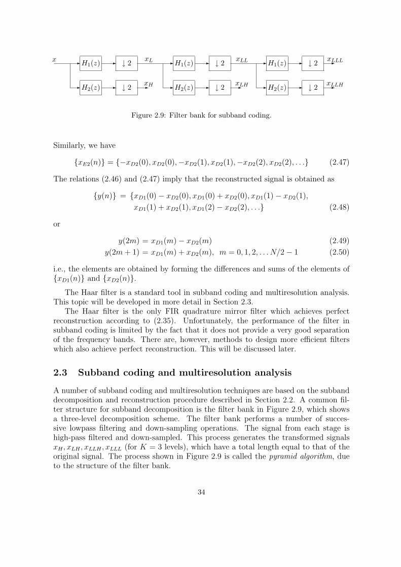
Figure 2.9: Filter bank for subband coding.

Similarly, we have

{xE2(n)} = {−xD2(0), xD2(0),−xD2(1), xD2(1),−xD2(2), xD2(2), . . .} (2.47)

The relations (2.46) and (2.47) imply that the reconstructed signal is obtained as

{y(n)} = {xD1(0)− xD2(0), xD1(0) + xD2(0), xD1(1)− xD2(1),

xD1(1) + xD2(1), xD1(2)− xD2(2), . . .} (2.48)

or

y(2m) = xD1(m)− xD2(m) (2.49)

y(2m + 1) = xD1(m) + xD2(m), m = 0, 1, 2, . . . N/2− 1 (2.50)

i.e., the elements are obtained by forming the differences and sums of the elements of{xD1(n)} and {xD2(n)}.

The Haar filter is a standard tool in subband coding and multiresolution analysis.This topic will be developed in more detail in Section 2.3.

The Haar filter is the only FIR quadrature mirror filter which achieves perfectreconstruction according to (2.35). Unfortunately, the performance of the filter insubband coding is limited by the fact that it does not provide a very good separationof the frequency bands. There are, however, methods to design more efficient filterswhich also achieve perfect reconstruction. This will be discussed later.

2.3 Subband coding and multiresolution analysis

A number of subband coding and multiresolution techniques are based on the subbanddecomposition and reconstruction procedure described in Section 2.2. A common fil-ter structure for subband decomposition is the filter bank in Figure 2.9, which showsa three-level decomposition scheme. The filter bank performs a number of succes-sive lowpass filtering and down-sampling operations. The signal from each stage ishigh-pass filtered and down-sampled. This process generates the transformed signalsxH , xLH , xLLH , xLLL (for K = 3 levels), which have a total length equal to that of theoriginal signal. The process shown in Figure 2.9 is called the pyramid algorithm, dueto the structure of the filter bank.

34

The filters H1 and H2 are often taken as the Haar filters (2.39) and (2.40), i.e.,

H1(z) =1

2

(z + 1

)(2.51)

H2(z) =1

2

(z − 1

)(2.52)

Referring to Figures 2.8 and 2.9, the original signal in Figure 2.9 is obtained recursivelyas

xLL(z) = G1(z)vLLL + G2(z)vLLH

xL(z) = G1(z)vLL + G2(z)vLH (2.53)

x(z) = G1(z)vL + G2(z)vH

where G1 = 1+z−1 and G2 = −1+z−1 (cf. (2.39) and (2.40)), and vLLL, vLLH , . . . denotethe up-sampled versions of xLLL, xLLH , . . .. By construction of the filters H1, H2, G1

and G2, perfect reconstruction of the original signal x is achieved.Recall from Section 2.2 that the filter H1(z) forms the average of two successive

signal values, so that the function of H1(z) followed by down-sampling is equivalent toforming pairwise averages of the signal. It follows that the low-pass filtered signals inFigure 2.9 are given by

xL(m) =1

2

(x(2m + 1) + x(2m)

)

xLL(m) =1

2

(xL(2m + 1) + xL(2m)

)

=1

4

(x(4m + 3) + x(4m + 2) + x(4m + 1) + x(4m)

)

xLL(m) =1

8

(x(8m + 7) + x(8m + 6) + x(8m + 5) + x(8m + 4)

+x(8m + 3) + x(8m + 2) + x(8m + 1) + x(8m))

and, thus, they define signal averages at various resolutions. Similarly, the filter H2(z)followed by down-sampling is equivalent to forming pairwise differences of the signalvalues. Hence

xH(m) =1

2

(x(2m + 1)− x(2m)

)

xLH(m) =1

2

(xL(2m + 1)− xL(2m)

)(2.54)

xLLH(m) =1

2

(xLL(2m + 1)− xLL(2m)

)

and the components xH , xLH and xLLH therefore describe the variation of the signal xat various resolutions. The decomposition described here is called Haar multiresolution.

35

-

6

Time

Frequency

N0

0

π

π/2

π/4

xH

xLH

xLLH

xLLL

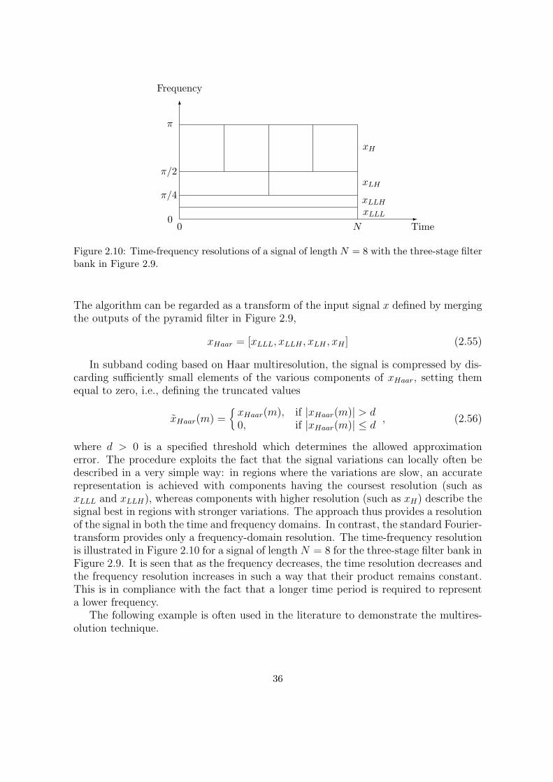
Figure 2.10: Time-frequency resolutions of a signal of length N = 8 with the three-stage filterbank in Figure 2.9.

The algorithm can be regarded as a transform of the input signal x defined by mergingthe outputs of the pyramid filter in Figure 2.9,

xHaar = [xLLL, xLLH , xLH , xH ] (2.55)

In subband coding based on Haar multiresolution, the signal is compressed by dis-carding sufficiently small elements of the various components of xHaar, setting themequal to zero, i.e., defining the truncated values

xHaar(m) ={

xHaar(m), if |xHaar(m)| > d0, if |xHaar(m)| ≤ d

, (2.56)

where d > 0 is a specified threshold which determines the allowed approximationerror. The procedure exploits the fact that the signal variations can locally often bedescribed in a very simple way: in regions where the variations are slow, an accuraterepresentation is achieved with components having the coursest resolution (such asxLLL and xLLH), whereas components with higher resolution (such as xH) describe thesignal best in regions with stronger variations. The approach thus provides a resolutionof the signal in both the time and frequency domains. In contrast, the standard Fourier-transform provides only a frequency-domain resolution. The time-frequency resolutionis illustrated in Figure 2.10 for a signal of length N = 8 for the three-stage filter bank inFigure 2.9. It is seen that as the frequency decreases, the time resolution decreases andthe frequency resolution increases in such a way that their product remains constant.This is in compliance with the fact that a longer time period is required to representa lower frequency.

The following example is often used in the literature to demonstrate the multires-olution technique.

36

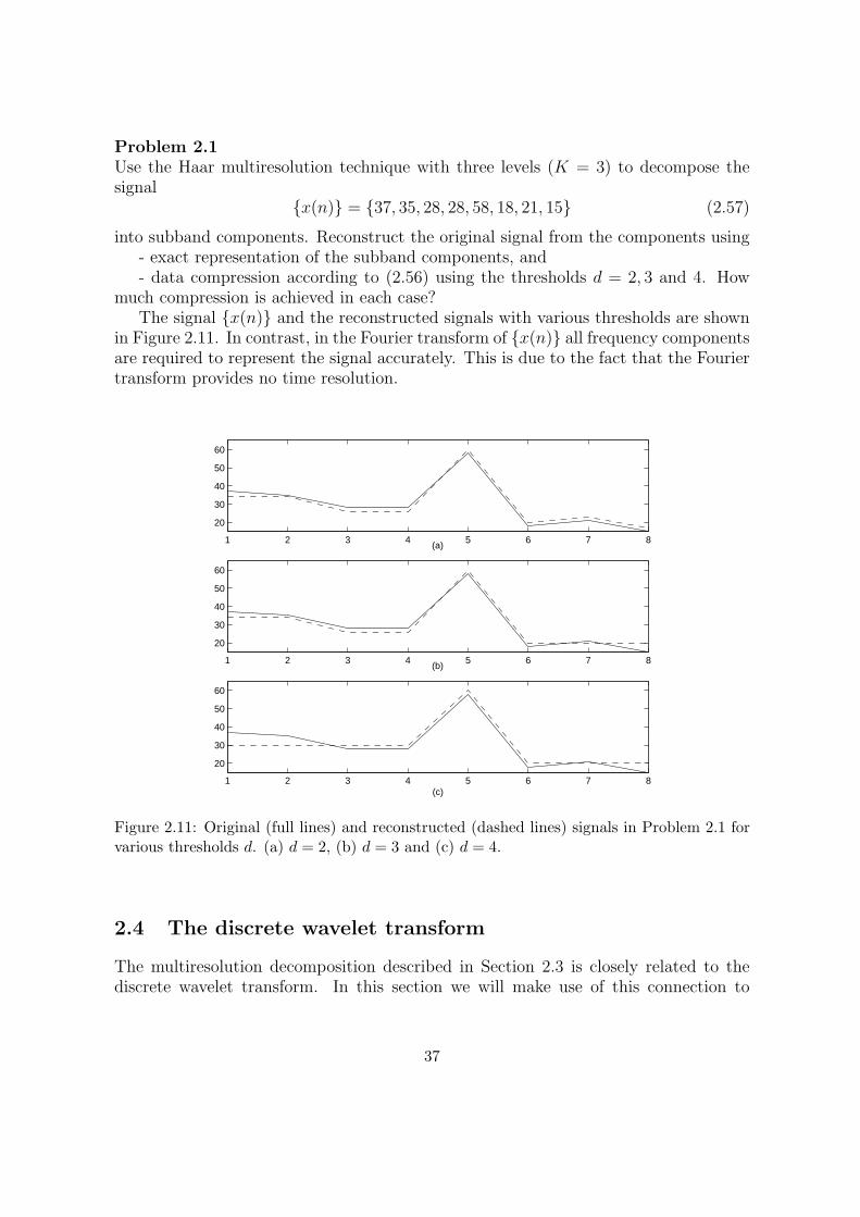
Problem 2.1Use the Haar multiresolution technique with three levels (K = 3) to decompose thesignal

{x(n)} = {37, 35, 28, 28, 58, 18, 21, 15} (2.57)

into subband components. Reconstruct the original signal from the components using- exact representation of the subband components, and- data compression according to (2.56) using the thresholds d = 2, 3 and 4. How

much compression is achieved in each case?The signal {x(n)} and the reconstructed signals with various thresholds are shown

in Figure 2.11. In contrast, in the Fourier transform of {x(n)} all frequency componentsare required to represent the signal accurately. This is due to the fact that the Fouriertransform provides no time resolution.

1 2 3 4 5 6 7 8

20

30

40

50

60

(a)

1 2 3 4 5 6 7 8

20

30

40

50

60

(b)

1 2 3 4 5 6 7 8

20

30

40

50

60

(c)

Figure 2.11: Original (full lines) and reconstructed (dashed lines) signals in Problem 2.1 forvarious thresholds d. (a) d = 2, (b) d = 3 and (c) d = 4.

2.4 The discrete wavelet transform

The multiresolution decomposition described in Section 2.3 is closely related to thediscrete wavelet transform. In this section we will make use of this connection to

37

characterize the discrete wavelet transform in terms of the pyramid filter bank in Figure2.9.

A discrete wavelet expansion of a signal {x(n)} of length N is defined as

x(n) =N/2J−1∑

m=0

XDWT (0,m)φ(2−Jn−m) +J∑

i=1

N/2i−1∑

m=0

XDWT (i,m)ψ(2−in−m) (2.58)

where φ(t) and ψ(t) are given functions (wavelets), and the set of coefficients XDWT (m, i)is the discrete wavelet transform (DWT) of the signal {x(n)}. A characteristic featureof the expansion (2.58) is that the signal is expanded in terms of the functions φ(t) andψ(t) as well as dilated (or stretched) and translated copies of the function ψ(t). Noticethat if ψ(t) is defined for 0 ≤ t < 1, and is zero elsewhere, then:

- ψ(2−in) is defined for 0 ≤ n < 2i, and is thus a dilated (stretched) version of ψ(t),- ψ(2−in−m) is defined for m2i ≤ n < (m + 1)2i, and is thus a dilated and translated

version of ψ(t).

The situation is illustrated in Figure 2.12, which shows a function together with adilated and a dilated and translated copies of it. In standard wavelet jargon, φ(t) isthe father wavelet, ψ(t) is the mother wavelet, and the dilated and translated copiesψ(2−in−m) are called daughter wavelets.

The number J in (2.58) defines the number of resolution levels. For a signal oflength N = 2K , J ≤ K.

By its construction, and in analogy with the multiresolution decomposition in Sec-tion 2.3, the wavelet transform provides a resolution of the signal in both the timeand frequency domains. It turns out that the wavelet transform in (2.58) can be char-acterized in terms of a pyramid filter bank of the form shown in Figure 2.9 (withJ = 3). Here, the filters H1(z) and H2(z) are associated with the father and motherwavelets φ(t) and ψ(t), respectively, the down-samplers describe dilation by the fac-tor two, and the discrete wavelet transform XDWT (i,m) consists of the filter outputsxLLL, xLLH , xLH , xH . The perfect reconstruction condition ensures that the originalsignal x can be expressed in terms of the transform according to (2.58).

The connection between multiresolution filter banks and wavelets will be exploredin more detail below. In Section 2.4.1 it is first shown that the Haar multiresolutiondescribed in Section 2.3 can be characterized as a wavelet transform. The result pavesthe way to the more general Daubechies wavelets which will be described in Section2.4.2.

2.4.1 Haar wavelets

In order to introduce the Haar wavelet, consider how the original signal x in Figure 2.9is reconstructed from the components xH , xLH , xLLH and xLLL. Referring to Section2.2 and Figure 2.8, we have (cf. equation (2.49))

xLL(2m) = xLLL(m)− xLLH(m)

xLL(2m + 1) = xLLL(m) + xLLH(m), (2.59)

38

m = 0, 1, . . . , N/2− 1. Similarly,

xL(4m) = xLL(2m)− xLH(2m)

= xLLL(m)− xLLH(m)− xLH(2m)

xL(4m + 1) = xLL(2m) + xLH(2m)

= xLLL(m)− xLLH(m) + xLH(2m)

xL(4m + 2) = xLL(2m + 1)− xLH(2m + 1)

= xLLL(m) + xLLH(m)− xLH(2m + 1) (2.60)

xL(4m + 3) = xLL(2m + 1) + xLH(2m + 1)

= xLLL(m) + xLLH(m) + xLH(2m + 1),

m = 0, 1, . . . , N/4− 1. Finally, the signal x is reconstructed according to

x(8m) = xL(4m)− xH(4m)

x(8m + 1) = xL(4m) + xH(4m)

x(8m + 2) = xL(4m + 1)− xH(4m + 1)

x(8m + 3) = xL(4m + 1) + xH(4m + 1)

x(8m + 4) = xL(4m + 2)− xH(4m + 2)

x(8m + 5) = xL(4m + 2) + xH(4m + 2)

x(8m + 6) = xL(4m + 3)− xH(4m + 3)

x(8m + 7) = xL(4m + 3) + xH(4m + 3)

Introducing the expressions from (2.60) gives

x(8m) = xLLL(m)− xLLH(m)− xLH(2m)− xH(4m)

x(8m + 1) = xLLL(m)− xLLH(m)− xLH(2m) + xH(4m)

x(8m + 2) = xLLL(m)− xLLH(m) + xLH(2m)− xH(4m + 1)

x(8m + 3) = xLLL(m)− xLLH(m) + xLH(2m) + xH(4m + 1)

x(8m + 4) = xLLL(m) + xLLH(m)− xLH(2m + 1)− xH(4m + 2)

x(8m + 5) = xLLL(m) + xLLH(m)− xLH(2m + 1) + xH(4m + 2)

x(8m + 6) = xLLL(m) + xLLH(m) + xLH(2m + 1)− xH(4m + 3)

x(8m + 7) = xLLL(m) + xLLH(m) + xLH(2m + 1) + xH(4m + 3),

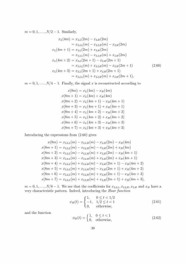
m = 0, 1, . . . , N/8− 1. We see that the coefficients for xLLL, xLLH , xLH and xH have avery characteristic pattern. Indeed, introducing the Haar function

ψH(t) =

1, 0 ≤ t < 1/2−1, 1/2 ≤ t < 10, otherwise,

(2.61)

and the function

φH(t) ={

1, 0 ≤ t < 10, otherwise,

(2.62)

39

we see that x can be expressed as

x(n) =N/23−1∑

i=0

xLLL(i)φH(2−3n− i)−N/23−1∑

i=0

xLLH(i)ψH(2−3n− i)

−N/22−1∑

i=0

xLH(i)ψH(2−2n− i)−N/2−1∑

i=0

xH(i)ψH(2−1n− i) (2.63)

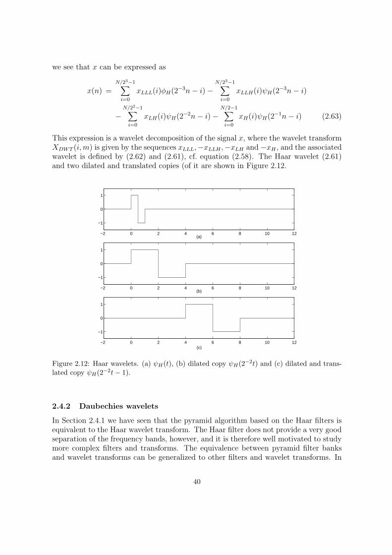
This expression is a wavelet decomposition of the signal x, where the wavelet transformXDWT (i, m) is given by the sequences xLLL,−xLLH ,−xLH and −xH , and the associatedwavelet is defined by (2.62) and (2.61), cf. equation (2.58). The Haar wavelet (2.61)and two dilated and translated copies (of it are shown in Figure 2.12.

−2 0 2 4 6 8 10 12

−1

0

1

(a)

−2 0 2 4 6 8 10 12

−1

0

1

(b)

−2 0 2 4 6 8 10 12

−1

0

1

(c)

Figure 2.12: Haar wavelets. (a) ψH(t), (b) dilated copy ψH(2−2t) and (c) dilated and trans-lated copy ψH(2−2t− 1).

2.4.2 Daubechies wavelets

In Section 2.4.1 we have seen that the pyramid algorithm based on the Haar filters isequivalent to the Haar wavelet transform. The Haar filter does not provide a very goodseparation of the frequency bands, however, and it is therefore well motivated to studymore complex filters and transforms. The equivalence between pyramid filter banksand wavelet transforms can be generalized to other filters and wavelet transforms. In

40

order to obtain a satisfactory wavelet transform, the associated filter bank should havethe following properties:

- The filters H1(z) and H2(z) should be FIR filters, and they should provide a goodfrequency separation,

- the filters H1(z) and H2(z) should be related in such a way that the filter bankgenerates a wavelet expansion of the form (2.58) for some wavelet function φ(t) andψ(t).

- the filter bank should have the perfect reconstruction property.

It is not at all evident that the above conditions can be satisfied. Recall for examplefrom Section 2.2 that the Haar filter is the only FIR quadrature mirror filter whichachieves the perfect reconstruction property. The fact that there does indeed exist aclass of filters which satisfy the conditions has been shown in a remarkable result byIngrid Daubechies (1988).

In order to present the Daubechies wavelets and the associated filter bank, recallthe signal decomposition according to Figure 2.8. For alias elimination, we require that(2.28) holds, and select the synthesis filters as

G1(z) = z−MH2(−z) (2.64)

G2(z) = −z−MH1(−z) (2.65)

where the time delay z−M is introduced in order to avoid a time advance in the recon-struction process. In contrast to Section 2.2, the analysis filters H1(z) and H2(z) willnot be selected to satisfy the quadrature mirror symmetry property (2.31). Instead, itcan be shown that the filter bank corresponds to a wavelet transform if the filters arechosen to satisfy

H2(z) = −zMH1(−z−1) (2.66)

where M is the order of H1(z) (so that the number of coefficients of the FIR filterH1(z) is M + 1). Daubechies filters are only defined for odd values of M . Combiningthe relations (2.64)–(2.66) gives

H1(z) = H(z)

H2(z) = −zMH(−z−1) (2.67)

G1(z) = H(z−1) (M odd)

G2(z) = −z−MH(−z)

More explicitly, ifH(z) = h0 + h1z + h2z

2 + · · ·+ hMzM , (2.68)

(2.67) implies

H1(z) = h0 + h1z + h2z2 + · · ·+ hMzM

H2(z) = −h0zM + h1z

M−1 − h2zM−2 + · · ·+ hM (2.69)

G1(z) = h0 + h1z−1 + h2z

−2 + · · ·+ hMz−M

G2(z) = −h0z−M + h1z

−M+1 − h2z−M+2 + · · ·+ hM

41

Notice the symmetries between H1(z) and G1(z), and H2(z) and G2(z). From (2.27)it follows that in order to achieve perfect reconstruction, we should have

1

2

(G1(z)H1(z) + G2(z)H2(z)

)= 1 (2.70)

Introducing (2.67) it follows that (2.70) implies the following condition on H1(z) =H(z):

1

2

(H(z)H(z−1) + H(−z)H(−z−1)

)= 1 (2.71)

D The problem has thus been reduced to finding a FIR filter H(z) which satisfies(2.71). It turns out that the solutions of (2.71) have the form

H(z) =√

2(

1 + z

2

)m

S(z) (2.72)

where S(z) is a FIR filter, which is normalized so that S(1) = 1, i.e., the filter S(z)has a unit stationary gain. It can be shown (after some algebraic manipulations) thatthe perfect reconstruction condition (2.71) implies that S(z) should satisfy

|S(ejω)|2 =m−1∑

k=0

(m + k − 1

k

)sin2k

(ω

2

)(2.73)

It turns out that for m = 1, 2, 3, . . ., equation (2.73) has a polynomial solution S(z) oforder m−1. It follows that the FIR filters H(z) in (2.72) have orders M = m+m−1 =2m− 1, i.e., M = 1, 3, 5, . . .. Notice that for the case m = 1, H(z) reduces to the Haarfilter (scaled by the factor

√2).

In analogy with the Haar filter, the filters (2.72) generate a wavelet transform whenapplied in a pyramid filter bank. The associated wavelet is called the Daubechieswavelet of order m = 1, 2, 3, . . .. The Haar wavelet discussed above is thus the simplestDaubechies wavelet, corresponding to m = 1.

Example 2.3 The Daubechies wavelet of order 2.As an example, consider the Daubechies wavelet of order m = 2. Some algebra showsthat equation (2.73) has the solution

S(z) =1−√3

2+

√3 + 1

2z (2.74)

By (2.72), H(z) is then given by

H(z) =√

2

{1−√3

8+

3−√3

8z +

3 +√

3

8z2 +

1 +√

3

8z3

}

= −0.129409522551 + 0.224143868042z + 0.836516303738z2 + 0.482962913145z3

42

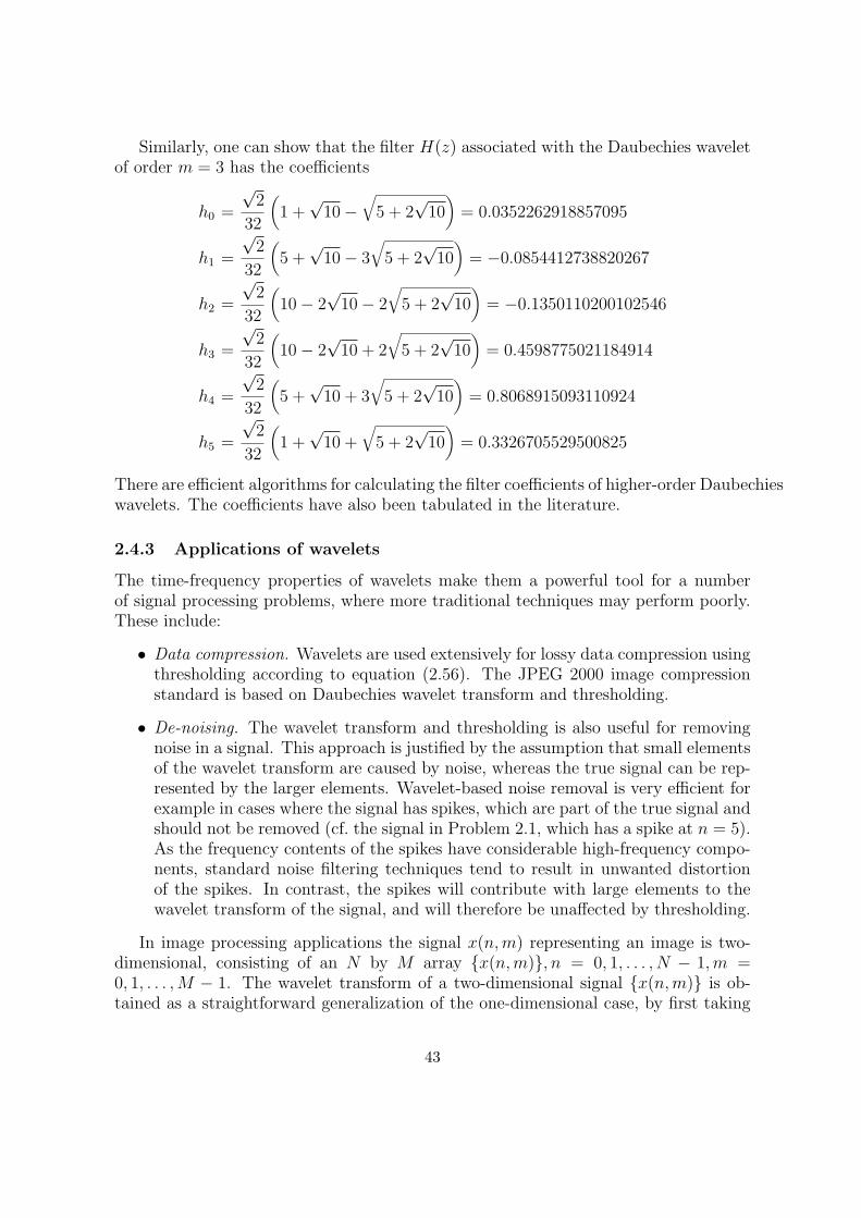
Similarly, one can show that the filter H(z) associated with the Daubechies waveletof order m = 3 has the coefficients

h0 =

√2

32

(1 +

√10−

√5 + 2

√10

)= 0.0352262918857095

h1 =

√2

32

(5 +

√10− 3

√5 + 2

√10

)= −0.0854412738820267

h2 =

√2

32

(10− 2

√10− 2

√5 + 2

√10

)= −0.1350110200102546

h3 =

√2

32

(10− 2

√10 + 2

√5 + 2

√10

)= 0.4598775021184914

h4 =

√2

32

(5 +

√10 + 3

√5 + 2

√10

)= 0.8068915093110924

h5 =

√2

32

(1 +

√10 +

√5 + 2

√10

)= 0.3326705529500825

There are efficient algorithms for calculating the filter coefficients of higher-order Daubechieswavelets. The coefficients have also been tabulated in the literature.

2.4.3 Applications of wavelets

The time-frequency properties of wavelets make them a powerful tool for a numberof signal processing problems, where more traditional techniques may perform poorly.These include:

• Data compression. Wavelets are used extensively for lossy data compression usingthresholding according to equation (2.56). The JPEG 2000 image compressionstandard is based on Daubechies wavelet transform and thresholding.

• De-noising. The wavelet transform and thresholding is also useful for removingnoise in a signal. This approach is justified by the assumption that small elementsof the wavelet transform are caused by noise, whereas the true signal can be rep-resented by the larger elements. Wavelet-based noise removal is very efficient forexample in cases where the signal has spikes, which are part of the true signal andshould not be removed (cf. the signal in Problem 2.1, which has a spike at n = 5).As the frequency contents of the spikes have considerable high-frequency compo-nents, standard noise filtering techniques tend to result in unwanted distortionof the spikes. In contrast, the spikes will contribute with large elements to thewavelet transform of the signal, and will therefore be unaffected by thresholding.

In image processing applications the signal x(n,m) representing an image is two-dimensional, consisting of an N by M array {x(n,m)}, n = 0, 1, . . . , N − 1, m =0, 1, . . . , M − 1. The wavelet transform of a two-dimensional signal {x(n,m)} is ob-tained as a straightforward generalization of the one-dimensional case, by first taking

43

the transform of each row, followed by the transform of each column. More pre-cisely, first each row of {x(n, m)} is transformed to give the array XDWT,row(n, k),where the nth row XDWT,row(n, k), k = 0, 1, . . . ,M − 1, is the transform of the one-dimensional signal consisting of the nth row x(n,m),m = 0, 1, . . . , M − 1. Then eachcolumn of XDWT,row(n, k) is transformed to give XDWT (l, k), where the kth columnXDWT (l, k), l = 0, 1, . . . , N − 1, is the transform of the one-dimensional signal consist-ing of the kth column XDWT,row(n, k), n = 0, 1, . . . , N − 1.

Efficient software exists for wavelet analysis. A library of MATLAB routines for waveletcalculations is available at http://www-stat.stanford.edu/~wavelab/.

44