Multiple View GeometryMultiple View Geometry

Projective Geometry Projective Geometry & &

Transformations of 2DTransformations of 2D

Vladimir NedovićVladimir Nedović

18-01-200818-01-2008

Intelligent Systems Lab Amsterdam (ISLA)Intelligent Systems Lab Amsterdam (ISLA)Informatics Institute, University of AmsterdamInformatics Institute, University of Amsterdam

Kruislaan 403, 1098 SJ Amsterdam, The NetherlandsKruislaan 403, 1098 SJ Amsterdam, The Netherlands

vnedovic@science.uva.nlvnedovic@science.uva.nl

OutlineOutline

Intro to projective geometryIntro to projective geometry

The 2D projective planeThe 2D projective plane

Projective transformationsProjective transformations

Hierarchy of transformationsHierarchy of transformations

Projective geometry of 1DProjective geometry of 1D

Recovery of affine & metric properties from imagesRecovery of affine & metric properties from images

More properties of conicsMore properties of conics

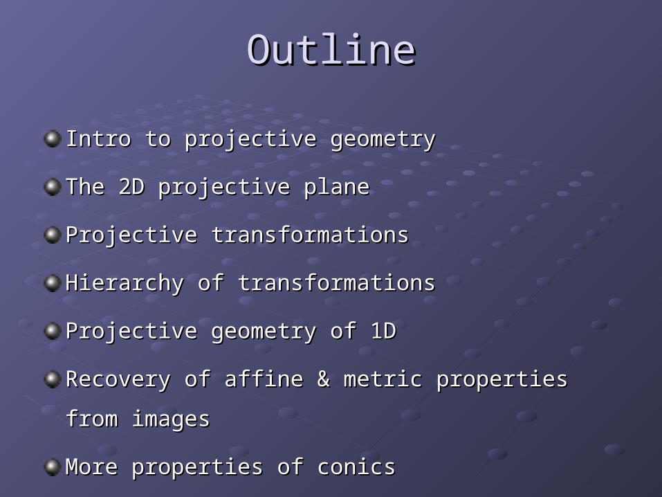
Intro to Projective GeometryIntro to Projective Geometry

Projective transformation: any mapping of points in Projective transformation: any mapping of points in the plane that preserves straight linesthe plane that preserves straight lines

Projective space: an extension of a Euclidean space Projective space: an extension of a Euclidean space in which two lines in which two lines alwaysalways meet in a point meet in a point parallel lines meet at inf. => no parallelism in proj. spaceparallel lines meet at inf. => no parallelism in proj. space

x = x/1y = y/1

homogeneouscoordinates in P2

(x,y,0) = (x/0,y/0,0) = (∞,∞,0)

points atinfinity

coordinates in Euclidean R2

(x,y) = (x,y,1) = (kx,ky,k) k ≠ 0

Intro to Projective Geometry (cont.)Intro to Projective Geometry (cont.)

Euclidean/affine transformation of Euclidean space:Euclidean/affine transformation of Euclidean space:

points at infinity remain at infinitypoints at infinity remain at infinity

≠Projective transformation of projective space:Projective transformation of projective space:

points at infinity map to arbitrary pointspoints at infinity map to arbitrary points

x’ = H x

(n+1)x(n+1)non-singular matrix

a point in Pn,an (n+1) - vector

In In PP22, points at infinity form a line, in , points at infinity form a line, in PP33 a plane, etc. a plane, etc.

e.g. an image of the real 3D world

e.g. the real3D world

The 2D projective planeThe 2D projective plane

Line Line l l in the plane: in the plane: ax + by + c = 0– equiv. to in slope-intercept notationequiv. to in slope-intercept notation

– thus a line could be represented by a vector thus a line could be represented by a vector (a,b,c)(a,b,c)TT

b

cx

b

ay

A point A point xx lies on line lies on line l l iffiff

ax + by + c = (x,y,1)(a,b,c)T = xTl = 0

Lines and points represented by Lines and points represented by homogeneoushomogeneous vectors vectors

(a,b,c)T = k(a,b,c)T

(x,y)T = k(x,y)T k ≠ 0

The 2D projective plane (cont.)The 2D projective plane (cont.)

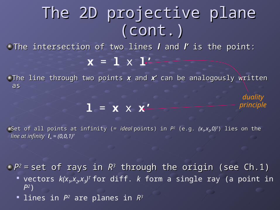
The intersection of two lines The intersection of two lines ll and and l’l’ is the point: is the point:x = l x l’

The line through two points The line through two points xx and and x’x’ can be analogously written as can be analogously written as

l = x x x’duality

principle

Set of all points at infinity (= Set of all points at infinity (= ideal ideal points) in points) in PP22 (e.g. (e.g. (x1,x2,0)T) lies on the ) lies on the line at infinityline at infinity ll∞ = (0,0,1)T

PP22 = = set of rays in set of rays in RR33 through the origin (see Ch.1) through the origin (see Ch.1) vectors k(x1,x2,x3)T for diff. k form a single ray (a point in P2) lines in P2 are planes in RR33

The 2D The 2D projective projective plane plane

(cont.)(cont.)

Ω

Λ

ll’idealpoint r1 = k(x1,x2,x3)

r2 = k(x1’,x2’,x3’)r1

r2

x1x2-plane ≡ l≡ l∞ ≡ ≡ Ω

l’ є Ω

l, l’, r1, r2 є Λ

θ

θ

Fig 2.1(extended)

lines in lines in PP22 are planes are planes e.g. line e.g. line ll is plane is plane Λ

x2

x1θ

x3 = 1

points in points in PP22 = = rays through rays through the originthe origin

point point xx11 = ray = ray rr11

The 2D projective plane (cont.)The 2D projective plane (cont.)

Duality principleDuality principle for 2D projective geometry for 2D projective geometry– for every theorem there is a dual one, obtained by for every theorem there is a dual one, obtained by

interchanging the roles of points and linesinterchanging the roles of points and lines

fed

ecb

dba

2/2/

2/2/

2/2/

C

A curve in Euclidean space corresponds to A curve in Euclidean space corresponds to a a conicconic in projective space in projective space

– defined using points:defined using points: xxTTCCxx = 0 = 0CC is a homog. representation, only is a homog. representation, only

the ratios of elements matterthe ratios of elements matter

– defined using (tangent) lines: defined using (tangent) lines: llTTCC-1-1ll = 0 = 0via the equation of a conic tangent at via the equation of a conic tangent at xx: : ll = C = Cxx

CC-1-1 only if only if CC non-singular, otherwise non-singular, otherwise C*C*

if if CC not of full rank, the conic is degenerate not of full rank, the conic is degenerate

Projective transformationsProjective transformationsRemember slide 1? Remember slide 1? ProjectivityProjectivity = = homographyhomography

= invertible mapping in = invertible mapping in PP22 that preserves linesthat preserves lines

– algebraically, mapping described by algebraically, mapping described by thethe matrix matrix HHagain only element ratios matter => again only element ratios matter => HH = = homogeneoushomogeneous matrix matrix

– leaves all projective properties of the figure leaves all projective properties of the figure invariantinvariant

x1

x1’

Fig. 2.3(extended)

central projectionpreserves lines => a projectivity

Projective transformations (cont.)Projective transformations (cont.)

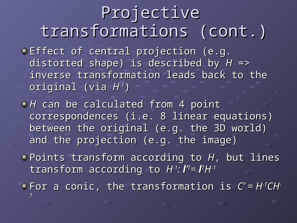
Effect of central projection (e.g. distorted shape) Effect of central projection (e.g. distorted shape) is described by is described by HH => inverse transformation => inverse transformation leads back to the original (via leads back to the original (via HH-1-1))

HH can be calculated from 4 point can be calculated from 4 point correspondences (i.e. 8 linear equations) correspondences (i.e. 8 linear equations) between the original (e.g. the 3D world) and the between the original (e.g. the 3D world) and the projection (e.g. the image)projection (e.g. the image)

Points transform according to Points transform according to HH, but lines , but lines transform according to transform according to HH-1-1: : ll’’TT= = llTTHH-1-1

For a conic, the transformation is For a conic, the transformation is C’ = HC’ = H-T-TCHCH-1-1

A hierarchy of transformationsA hierarchy of transformations

Projective transformations form a group, Projective transformations form a group, PL(3)PL(3)– characterized by invertible 3x3 matricescharacterized by invertible 3x3 matrices

In terms of increased specialization:In terms of increased specialization:

similarity affine projective

1. Isometry

2. Similarity

3. Affine

4. Projective

Can be described algebraically (i.e. via the transform matrix) or in Can be described algebraically (i.e. via the transform matrix) or in terms of invariantsterms of invariants

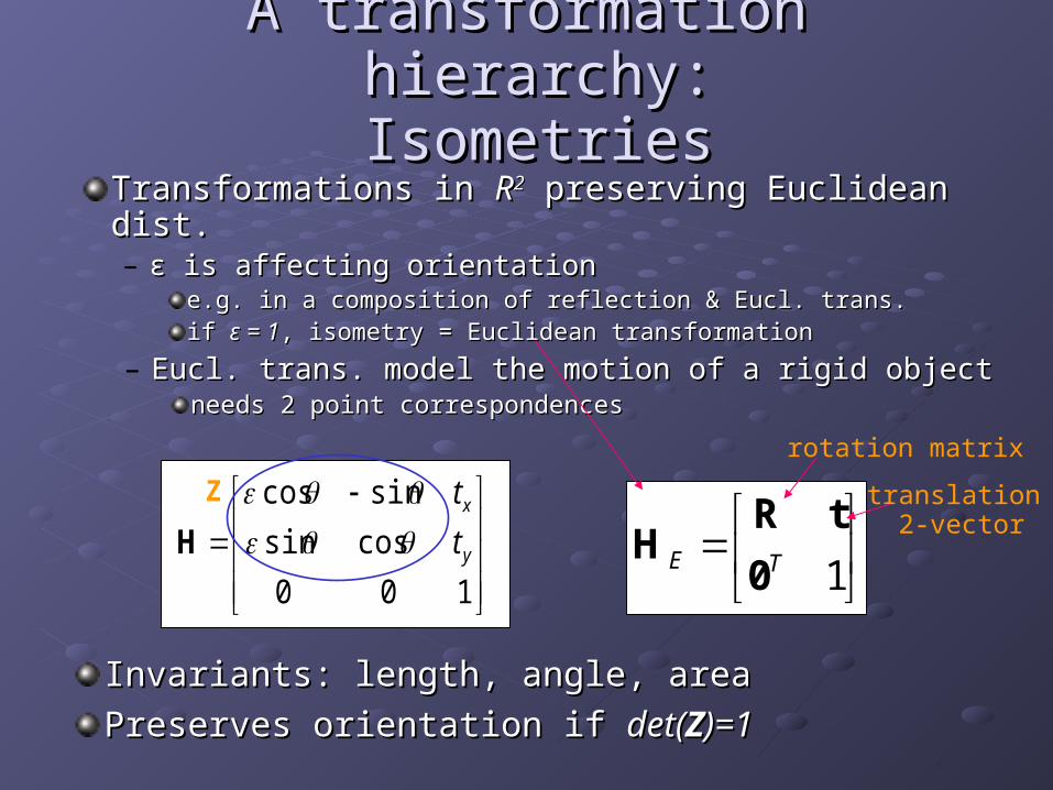
A transformation hierarchy: A transformation hierarchy: IsometriesIsometries

Transformations in Transformations in RR22 preserving Euclidean dist. preserving Euclidean dist.– εε is affecting orientationis affecting orientation

e.g. in a composition of reflection & Eucl. trans.e.g. in a composition of reflection & Eucl. trans.if if εε = 1 = 1, isometry = Euclidean transformation, isometry = Euclidean transformation

1TE 0

tRH

rotation matrix

translation 2-vector

Invariants: length, angle, areaInvariants: length, angle, area

Preserves orientation if Preserves orientation if det(det(ZZ)=1)=1

100

cossin

sincos

y

x

t

t

H

Z

– Eucl. trans. model the motion of a rigid objectEucl. trans. model the motion of a rigid objectneeds 2 point correspondencesneeds 2 point correspondences

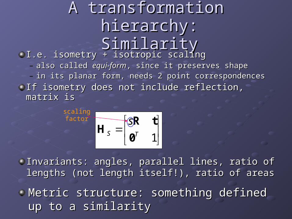
A transformation hierarchy: A transformation hierarchy: SimilaritySimilarity

I.e. isometry + isotropic scalingI.e. isometry + isotropic scaling– also called also called equi-formequi-form, since it preserves shape, since it preserves shape– in its planar form, needs 2 point correspondencesin its planar form, needs 2 point correspondences

If isometry does not include reflection, matrix isIf isometry does not include reflection, matrix is

1TS

s

0

tRH

scalingfactor

Invariants: angles, parallel lines, ratio of lengths Invariants: angles, parallel lines, ratio of lengths (not length itself!), ratio of areas(not length itself!), ratio of areas

Metric structure: something defined up to a Metric structure: something defined up to a similaritysimilarity

A transformation hierarchy: A transformation hierarchy: AffineAffine

Non-singular linear transformation + translationNon-singular linear transformation + translation– can be computed from 3 point correspondencescan be computed from 3 point correspondences– invariants: parallel lines, ratios of lengths of their segments, invariants: parallel lines, ratios of lengths of their segments,

ratio of areasratio of areas

1TA 0

tAH

2x2 non-singularmatrix defining

linear transformation

Can be thought of as the composition of rotations Can be thought of as the composition of rotations and non-isotropic scalingsand non-isotropic scalings– the affine matrix the affine matrix A A is thenis then

2

1

0

0

D

rotationby θ

scaling byλ1 and λ2

rotationby φ

rotationback by -φ

essence of affinity,separate scaling

in orthog. directions

AA = R( = R(θθ)R(-)R(-φφ)DR()DR(φφ),),

A transformation hierarchy: A transformation hierarchy: ProjectiveProjective

Most general linear trans. of homog. coords.Most general linear trans. of homog. coords.– i.e. the one that only preserves straight linesi.e. the one that only preserves straight lines– affine was as general, but in inhomogeneous coords.affine was as general, but in inhomogeneous coords.– requires 4 point correspondencesrequires 4 point correspondences– the block form of the matrix isthe block form of the matrix is

vTP v

tAH v = (v1,v2)T

(not null aswith affine =>

non-linear effects)

Invariants: cross-ratio of 4 collinear points (i.e. Invariants: cross-ratio of 4 collinear points (i.e. the ratio of ratios of line segments)the ratio of ratios of line segments)

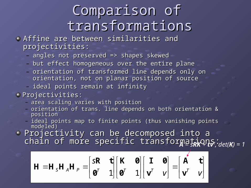
Comparison of transformationsComparison of transformations

Affine are between similarities and projectivities: Affine are between similarities and projectivities: – angles not preserved => shapes skewedangles not preserved => shapes skewed– but effect homogeneous over the entire planebut effect homogeneous over the entire plane– orientation of transformed line depends only on orientation, not orientation of transformed line depends only on orientation, not

on planar position of sourceon planar position of source– ideal points remain at infinityideal points remain at infinity

Projectivities:Projectivities:– area scaling varies with positionarea scaling varies with position– orientation of trans. line depends on both orientation & positionorientation of trans. line depends on both orientation & position– ideal points map to finite points (thus vanishing points modeled)ideal points map to finite points (thus vanishing points modeled)

Projectivity can be decomposed into a chain of more Projectivity can be decomposed into a chain of more specific transformations:specific transformations:

vv

sTTTTPAS v

tA

v

0I

0

0K

0

tRHHHH

11

A = sRK + tvT, det(K) = 1

Projective geometry of 1DProjective geometry of 1D

Very similar to 2DVery similar to 2D– proj. trans. of the plane implies a 1D proj. trans. of proj. trans. of the plane implies a 1D proj. trans. of

every line in the planeevery line in the plane

Proj. trans. for a line is a 2x2 homog. matrixProj. trans. for a line is a 2x2 homog. matrix– thus 3 point correspondences requiredthus 3 point correspondences required

Cross ratio is the basic projective invariant in 1DCross ratio is the basic projective invariant in 1D

423

432

432 ),,,(xxxx

xxxxxxxx

1

1

1 Cross

22

11det

ji

ji

ji xx

xxxx

signed distance from one to another

(if each is a finite point,and homog. coord. is 1)

Dual to collinear points are Dual to collinear points are concurrent lines, also having a concurrent lines, also having a PP11 geometrygeometry

Recovery of affine & metric Recovery of affine & metric properties from imagesproperties from images

Recover metric properties (i.e. up to a similarity)Recover metric properties (i.e. up to a similarity)1.1. by using 4 points to completely remove projective by using 4 points to completely remove projective

distortiondistortion

2.2. by identifying line at infinity by identifying line at infinity ll∞∞ and two circular points and two circular points

(i.e. their images)(i.e. their images)

Once Once ll∞∞ is identified in the image, affine is identified in the image, affine measurements can be made in the originalmeasurements can be made in the original

– e.g. parallel lines can be identified, length ratios e.g. parallel lines can be identified, length ratios computed, etc.computed, etc.

Affine is the most general trans. for which Affine is the most general trans. for which ll∞∞ remains a fixed lineremains a fixed line

– but point-wise correspondence achieved only if the but point-wise correspondence achieved only if the point is an eigenvector of point is an eigenvector of AA

Recovery of affine & metric Recovery of affine & metric properties from images (cont.)properties from images (cont.)

But identified But identified ll∞∞ can also be transformed to can also be transformed to ll∞∞ = (0,0,1)= (0,0,1)TT with a suitable proj. with a suitable proj.

matrixmatrix

– such a matrix could be such a matrix could be

321

010

001

lllAHH

– this matrix can then this matrix can then be applied to all be applied to all points, and affine points, and affine measurements measurements made in the made in the recovered imagerecovered image

Figure 2.12

Recovery of affine & metric Recovery of affine & metric properties from images (cont.)properties from images (cont.)

Beside the line at infinity, the two circular points Beside the line at infinity, the two circular points are fixed under similarityare fixed under similarity

– i.e. a pair of complex conjugatesi.e. a pair of complex conjugates– every circle intersects every circle intersects ll∞∞ at these at these

Metric rectification is possible if circular points Metric rectification is possible if circular points are transformed into their canonical positionsare transformed into their canonical positions

– applying the transformation to the entire image results applying the transformation to the entire image results in a similarityin a similarity

0

1

iI

0

1

iJ

The degenerate line conic is dual to circ. pointsThe degenerate line conic is dual to circ. points– once it is identified, Euclidean angles and length once it is identified, Euclidean angles and length

rations can be measuredrations can be measured– direct metric rectification also possibledirect metric rectification also possible

Properties of conicsProperties of conics

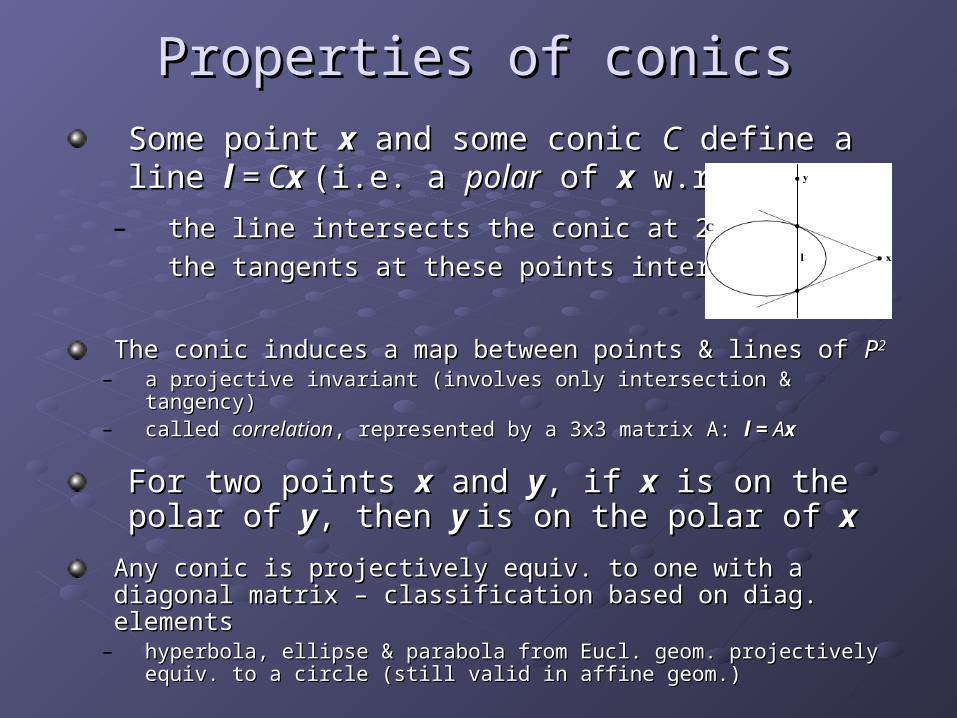
Some point Some point xx and some conic and some conic CC define a line define a line ll = C = Cx x (i.e. a (i.e. a polarpolar of of xx w.r.t. w.r.t. CC))

– the line intersects the conic at 2 points -> the line intersects the conic at 2 points ->

the tangents at these points intersect at the tangents at these points intersect at xx

The conic induces a map between points & lines of The conic induces a map between points & lines of PP22

– a projective invariant (involves only intersection & tangency)a projective invariant (involves only intersection & tangency)– called called correlationcorrelation, represented by a 3x3 matrix A: , represented by a 3x3 matrix A: l = l = AAxx

For two points For two points xx and and yy, if , if xx is on the polar of is on the polar of yy, then , then y y is on the polar of is on the polar of xx

Any conic is projectively equiv. to one with a diagonal Any conic is projectively equiv. to one with a diagonal matrix – classification based on diag. elementsmatrix – classification based on diag. elements

– hyperbola, ellipse & parabola from Eucl. geom. projectively hyperbola, ellipse & parabola from Eucl. geom. projectively equiv. to a circle (still valid in affine geom.)equiv. to a circle (still valid in affine geom.)

The End !The End !