Embed Size (px)
Citation preview
Multiple Risks and Mean-Variance Preferences
Thomas Eichnera and Andreas Wagenerb
a) Department of Economics, University of Bielefeld, Universitatsstr. 25, 33615 Biele-
feld, Germany. E-mail: [email protected]
b) Institute of Social Policy, University of Hannover, Koenigsgworther Platz 1, 30167
Hannover, Germany. E-mail: [email protected]
Subject classification: Decision analysis: Risk
Area of Review: Decision analysis
Abstract: We analyze comparative static effects under uncertainty when a decision maker
has mean-variance preferences and faces a generic, quasi-linear decision problem with both an
endogenous risk and a background risk. In terms of mean-variance preferences, we fully charac-
terize the effects of changes in the location, scale, and concordance parameters of the stochastic
environment on optimal risk-taking. Presupposing compatibility between mean-variance and
expected-utility approach we then translate these mean-variance properties into their analogues
for von-Neumann-Morgenstern utility functions.
2
1 Introduction
Comparative statics for decision problems with uncertainty over monetary outcomes have since
long found the interest of economists. Most of the numerous studies in that field operate within
the expected utility (EU) framework, the standard (but not entirely undisputed) approach to
rational choice under risk. The analyses encompass scenarios with single as well as with multiple
risks, and they set up generic decision models (Feder, 1977; Dionne et al., 1993; Bigelow and
Menezes, 1995) as well as specific applications for portfolio selection (Fishburn and Porter, 1976),
firm behaviour (Sandmo, 1971), insurance demand (Meyer, 1992; Hadar and Seo, 1992), hiring
under uncertainty (Feder, 1977), and many others.
Most prominent among the various alternatives to the EU-approach is mean-variance analysis1
which represents preferences over lotteries as functions of the mean and the variance or standard
deviation of final wealth. Since its (re-)invention2 by Markowitz (1952) and Tobin (1958), mean-
variance analysis has been highly popular both in economic theory (notably in the theory of
finance) and in practical applications. Its main merits are expository simplicity and an intuitive
interpretation: all effects can be couched in terms of risk and returns, and mean-variance models
remain two-dimensional even with multi-dimensional risks or choice variables.
In recent years mean-variance analysis has also re-gained some attention among theorists (Lajeri,
1995; Lajeri and Nielsen, 1995, 2000; Wagener, 2002; Eichner and Wagener, 2003a; Mathews,
2004). Yet, in spite of the widespread use of mean-variance analysis in theory and practice,
comparative static analyses in that framework are remarkably scant, both in absolute number
and relative to the EU-paradigm. They include an early graphical analysis of the behaviour of
the competitive firm under uncertainty by Hawawini (1978), a formal analysis of the portfolio
problem with a riskless and a risky asset by Lajeri-Chaherli (2003) and the analysis of linear
risk tolerance in Wagener (2005). Eichner and Wagener (2003a) employ the notion of variance
vulnerability to characterize the effects of changing an independent background risk in a generic
decision problem. Lajeri-Chaherli (2002, 2005) investigates the comparative statics of different
risk premia, employing risk-attitudes such as properness and standardness. In the standard1This approach comes under different labels: two-parameter approach, mean-standard deviation approach,
(µ, σ)-approach etc.2Markowitz (1999) provides a historical account of mean-variance analysis.
1
portfolio problem augmented by an independent background risk, Eichner (2007) shows that
the properties of properness and standardness also suffice for the comparative static effect of
increases in background risk.
In this paper, we aim at a systematic and comprehensive analysis of behavioural responses in
the mean-variance framework. For a generic decision problem with two risks we characterize
the comparative-static effects for the full set of distribution parameters (i.e., for the means,
variances, and the covariance of the two random variables). We trace back all comparative
static effects to simple and intuitive sensitivity or curvature properties of the marginal rates of
substitution between risk and return (i.e., of the willingness-to-pay for risk reductions). This is
the first contribution of this paper.
Generally, mean-variance and EU-approach constitute distinct frameworks for decision making
under risk (Ormiston and Schlee, 2001). The former is largely deemed deficient relative to the
latter (which derives much of its appeal from the underlying von-Neumann-Morgenstern [vNM]
axiomatization). However, in certain contexts, EU- and mean-variance approach are closely
related. In fact, they are perfect substitutes if (and only if) all attainable lotteries can, after
normalizing them by their means, be completely ordered by the Rothschild-Stiglitz criterion for
increases in risk (Bigelow, 1993). This concept of normalized risk comparability generalizes the
location-scale property which requires that attainable lotteries differ from one another only by
the mean and standard deviation of final wealth (Meyer, 1987; Sinn, 1983). In particular, it
applies when a single choice variable and a one-dimensional risk interact in a linear way — as
it happens in a wide range of important economic applications, encompassing the problems of
co-insurance, hedging, portfolio choice, liquidity demand, or output choices under uncertainty.3
For set-ups that possess the location-scale property, comparative-static effects in the mean-
variance framework have equivalent counterparts in terms of expected utility and vNM utility
indexes. Changes of means, variances and covariance correspond to first-order stochastic dom-
inance shifts, mean-preserving contractions, or changes in the concordance structure between
random variables. For the EU-framework, characterizations of the corresponding comparative3For multi-dimensional risks, the location-scale property is satisfied whenever final monetary outcomes result
from a linear combination of risks that jointly possess an elliptically symmetric distribution (Chamberlain, 1983;
Owen and Rabinovitch, 1983). For more on this, see Section 5.
2
statics are well-known from the literature (see Section 5 for an extensive discussion). We provide
“translations” of these characterizations in terms of the mean-variance approach. This is the
second contribution of this paper.
Naturally, characterizations of comparative-static effects derived in a mean-variance setup re-
main, once appropriately translated, valid also in the EU-framework on that subset of decision
problems where the two approaches are perfect substitutes. We exploit this observation to derive
new insights for the EU-framework via the detour of mean-variance analysis. E.g., comparative
statics of changes in background risks have so far only partly been analyzed within the EU-
framework proper. In particular, only little is known about the comparative statics of adding
(or, more generally, of increasing) dependent background risks.4 By contrast, the mean-variance
characterizations we establish for changes in background risks do not require any restriction
on the dependence structures between endogenous and background risks or on the presence or
absence of initial background uncertainty. Within the (reasonably general) location-scale frame-
work, the full (and yet simple) characterization of comparative statics for changes in dependent
risks, thus, generates new insights also for models of decision making using the EU-approach.
This is a third contribution of our paper.
We proceed as follows: Section 2 sets up a generic decision problem with mean-variance prefer-
ences. In Section 3 we characterize, in terms of restrictions on preferences, comparative static
effects for changes in each of the parameters of the risky environment. Section 4 clarifies the rela-
tion between EU- and mean-variance framework within the location-scale property and translates
the conditions obtained in Section 3 into their EU-analogues. Section 5 embeds these results
into the existing literature on the EU-approach. Section 6 concludes.4Lajeri-Chaherli (2002) and Eichner (2005) are exceptions. While Lajeri-Chaherli (2002) analyzes the addition
of a dependent risk on equivalent and compensating risk premia, Eichner (2005) studies the portfolio problem
with dependent background risk and points out that properness is sufficient for the comparative static effect of
increases in background risk.
3
2 Set-up
An individual decision maker chooses among different lotteries over his final wealth y. His
preferences for lotteries are represented by a two-parameter utility function
V : R+ × R → R, V = V (σy, µy), (1)
where σy ∈ R+ and µy ∈ R denote, respectively, the standard deviation and the expected value
of random final wealth y, calculated for an underlying probability distribution (that will most
often be suppressed in our notation). Generally, for a random variable ε we shall denote its
expected value by µε and its standard deviation by σε.
The preference functional V (σy, µy) is assumed to be at least four times continuously differen-
tiable, increasing in µy (non-satiation), decreasing in σy (risk aversion), and to exhibit strictly
convex indifference curves in (σy, µy)-space. Denoting partial derivatives with subscripts, we,
thus, require that the following properties are satisfied for all (σy, µy) ∈ R++ × R:5
Vµ(σy, µy) > 0; (2a)
Vσ(σy, µy) < 0; (2b)
V (σy, µy) is strictly quasi-concave in (σy, µy). (2c)
We denote by
m(σy, µy) := −Vσ(σy, µy)Vµ(σy, µy)
the marginal rate of substitution (MRS) between σy and µy. Lajeri and Nielsen (1995, 2000)
and Ormiston and Schlee (2001) identify m(σy, µy) as the two-parameter analogue of the Arrow-
Pratt concept of absolute risk aversion. Following Tobin (1958, p. 13) and Sinn (1983, pp. 112f.)
we assume that (σy, µy)-indifference curves enter the µy-axis with slope zero, representing risk
neutrality with respect to very small risks:
m(0, µy) = Vσ(0, µy) = 0 ∀µy ∈ R. (2d)
5As is shown in Eichner (2007, Proposition 3), quasi-concavity (2c) requires, for all (σy, µy),
−V 2σ · Vµµ + 2Vµ · Vσ · Vµσ − V 2
µ · Vσσ > 0.
4
We consider a class of decision problems where final wealth y is a function of a one-dimensional
and non-negative choice variable q ≥ 0. In particular, we assume the following quasi-linear form
of Feder (1977)’s general approach:
y(q) = x · q + f(q) + z. (3)
Both x and z are random variables. As the impact of q on the distribution of final wealth y
directly works through x, we call x the endogenous risk; the “passive” random variable z will
be referred to as the background risk. The interaction between the endogenous risk x and the
choice variable q is linear. The function f(q) is assumed to be smooth and concave in q, and to
satisfy f(0) = 0. This implies that f ′(q) · q − f(q) ≥ 0 for all q ≥ 0. Without loss of generality,
we assume that the expected value of z is non-negative.6
The dependence structure of endogenous risk x and background risk z is captured by their
covariance σxz := Cov(x, z), and the degree of their linear dependence is measured by the
Pearson coefficient of correlation ρ := σxz/(σx · σz) ∈ (−1, 1). Denote by
Θ := {(µx, µz, σx, σz, σxz) |µx ∈ R, µz, σx, σz ∈ R+,−σxσz ≤ σxz ≤ σxσz }
the set of possible parameters; a typical element of Θ will be denoted by θ.
Given (3), the expected value and the standard deviation of final wealth are given by:
µy(q) = µx · q + f(q) + µz (4)
σy(q) =√
σ2x · q2 + σ2
z + 2 · q · σxz. (5)
By an appropriate interpretation or re-definition of variables, specification (3) captures a wide ar-
ray of standard economic choice problems under risk: portfolio choice, saving under uncertainty,
insurance demand, output choices of competitive firms under uncertainty etc. To illustrate,
consider the following
Example: Portfolio choice with two assets. An individual has one unit of wealth which
has to be divided on two assets with (random) net returns a and b. Denote by µc and σc the6Alternatively, we could replace z by a random variable z + µz where z has expected value zero and include
µz in f as µz = f(0). This would be notationally slightly more inconvenient without affecting any results.
5

mean and standard deviations of returns c = a, b and by σab their covariance. With pa and pb
as the amounts that go, respectively, to assets a and b, final wealth y is given by
y(q) = pa · a + pb · b = qx + z
where we set q := pb = 1− pa and z := a. Moreover, x := b− a measures the difference between
the returns of the assets (and f(q) ≡ 0).7
Obviously, µx = µb − µa, σ2x = σ2
b + σ2a − 2σab, and σxz = σab − σ2
a (which is zero if and only if
return a is certain). Clearly,
µy(q) = µx · q + µz = pa · µa + pb · µb, (6a)
σy(q) =√
σ2x · q2 + σ2
z + 2 · q · σxz =√
p2a · σ2
a + p2b · σ2
b + 2 · pa · pb · σab. (6b)
Observe that this problem is structurally identical to a portfolio problem with one risky asset,
one safe asset, and some (possibly uncertain background) wealth (see Fishburn and Porter, 1976;
Eichner, 2007, on that problem).
Turning back to the general case, the decision maker solves the following problem:
maxq≥0
V (σy(q), µy(q)) subject to (4) and (5). (7)
Restricting attention to interior solutions of this program, the optimal level q∗ = q∗(θ) > 0,
where θ ∈ Θ, is then determined by the first-order condition
Φ (q∗, θ) = 0 (8)
where we set
Φ (q, θ) :=∂µy
∂q· Vµ(σy(q), µy(q)) +
∂σy(q)∂q
· Vσ(σy(q), µy(q))
=[µx + f ′(q)
]· Vµ(σy(q), µy(q)) +
∂σy(q)∂q
· Vσ(σy(q), µy(q)).
The second-order condition for a maximum8 is satisfied due to the quasi-concavity of V (σy, µy)
in (σy, µy) and the concavity of f(q) in q.7The reason for the redundany in notation will (hopefully) become clear below.8After some rearrangements, the second-order condition can be written as
Φq(q∗, θ) = −
(∂σy(q∗)
∂q
)2 (−V 2
σ Vµµ + 2VµVσVµσ − V 2µ Vσσ
V 2µ
)+ f ′′(q∗)Vµ +
σ2xσ2
z − σ2xz
σy(q∗)< 0.
6
We will henceforth assume that q denotes a risky activity in the sense that it marginally increases
the standard deviation of final wealth at its optimal level q∗:
∂σy(q∗)∂q
=σ2
x · q∗ + σxz
σy(q∗)> 0. (9)
From (8) this obviously implies that, at the optimal level, activity q marginally increases expected
final wealth, too: µx + f ′(q∗) > 0.
We wish to ensure that increases in σx or σz indeed constitute increases in risk, i.e., they lead
to an increase in the standard deviation of final wealth. This obviously holds whenever we keep
the dependence structure between x and z fixed upon a change in σx or σz; from (5),
∂σy(q∗)∂σx
> 0 and∂σy(q∗)
∂σz> 0
hold for all q∗ = q∗(θ). In addition we require that increases in the standard deviations of x and
z constitute increases in risks also if we keep their correlation fixed but allow their covariance
to vary. Rewriting the standard deviation of final wealth as
σy(q) =√
σ2x · q2 + σ2
z + 2 · q · ρ · σx · σz,
we require that
∂σy(q∗)∂σx
≥ 0 and∂σy(q∗)
∂σz> 0.
The first of these conditions is equivalent to (9), i.e., to the fact that q is a risky activity. The
second condition requires σz + q∗ρσx > 0 or
σ2z + q∗ · σxz > 0. (10)
This automatically holds whenever x and z are non-negatively correlated; for negative values of
σxz, condition (10) constitutes an assumption on its own.
Example (ctd.): To illustrate these assumptions, we return to the two-asset portfolio example
from above. It is straightforward to show that (9) and (10) are together equivalent to:
pb · σ2a + pa · σab > pa · σ2
b + pb · σab > 0
7
(where pa = 1− q∗ and pb = q∗ have to be evaluated at their optimal levels). From (6b), this is
tantamount to:
∂σy
∂pb>
∂σy
∂pa> 0.
Hence, both investments pa and pb are risky in the sense that independently increasing either
leads to higher overall risk. However, activity pb is (in the optimum) riskier than activity pa –
which, by the constraint that pb = q and pa = 1 − q must add up to unity, implies that q it-
self is a risk-increasing activity. Hence, conditions (9) and (10) have quite simple interpretations.
To summarize, we consider quasi-linear choice problems of type (3) where increases in the
standard deviations of the endogenous or of the background risk always lead to an increase in
overall risk (i.e., where (9) and (10) hold).
3 Comparative Statics
We are interested in how optimal risk-taking responds to changes in the stochastic parameters of
the decision problem. In this section we provide complete characterizations of the comparative
statics of q∗(θ) with respect to all components of θ.
3.1 Changes in the Background Risk
Our first result deals with the comparative statics for changes in the distribution of the back-
ground risk z:
Proposition 1.
a) An agent will, for all θ ∈ Θ, increase q∗(θ) upon an increase in µz if and only if mµ(σy, µy) <
0 for all (σy, µy).
b) An agent will, for all θ ∈ Θ, decrease q∗(θ) upon an increase in σz if and only if mσ(σy, µy) >
0 and mσσ(σy, µy) > 0 for all (σy, µy).
Proof: The first-order condition (8) can be rewritten as
Φ(q∗, θ) = Vµ ·[µx + f ′(q∗)− ∂σy(q∗)
∂q·m(σ∗y , µ
∗y)
]= 0. (11)
8
a) Implicit differentiation of (11) with respect to µz yields
∂q∗
∂µz= − Vµ
Φq(q∗, θ)·(−∂σy(q∗)
∂q
)·mµ(σ∗y , µ
∗y)
which is positive if and only if mµ(σ∗y , µ∗y) < 0 for all (σ∗y , µ
∗y) (recall assumption (9)).
b) Implicit differentiation of (11) with respect to σz yields, after some rearrangements,
∂q∗
∂σz= − Vµ
Φq(q∗, θ)· ∂σy(q∗)
∂q· σz
σ∗y·[m(σ∗y , µ
∗y)
σ∗y−mσ(σ∗y , µ
∗y)
](12)
which is negative if and only if
m(σ∗y , µ∗y)
σy−mσ(σ∗y , µ
∗y) < 0 (13)
for all (σ∗y , µ∗y).
Obviously, this necessitates mσ(σ∗y , µ∗y) > 0. Given this and (2d), condition (13) is equiv-
alent to mσσ(σ∗y , µ∗y) > 0. �
As shown by Lajeri and Nielsen (1995) and Ormiston and Schlee (2001), the slope of (σy, µy)-
indifference curves with respect to µy determines whether absolute risk aversion increases or
decreases. Formally, the more appealing property of decreasing absolute risk aversion (DARA)
is represented in the two-parameter framework by
mµ(σy, µy) < 0 ∀(σy, µy) ∈ R+ × R. (14)
Eichner and Wagener (2003a) show that convexity of the slope of (σy, µy)-indifference curves
with respect to σy, i.e.,
mσσ(σy, µy) > 0 ∀(σy, µy) ∈ R+ × R, (15)
together with mσ(σy, µy) > 0, generally characterizes the comparative static effect that individ-
uals behave in a more-risk averse way when they are confronted with an increase in an inde-
pendent background risk. Inspired by the concept of “risk vulnerability” in the expected-utility
framework, Eichner and Wagener (2003a) refer to property (15) as variance vulnerability.9
9Note that mσ(σy, µy) > 0 and the convexity of the indifference curves (2c) together imply that mµ(σy, µy) < 0
(see also Lajeri-Chaherli, 2003, p. 90). Hence, DARA is a necessary condition for variance vulnerability. Variance
9
In short, Proposition 1 conveys that the individual behaves in a less risk-averse way when facing
an increase in the expected value of the (possibly degenerate) background risk or a decrease
in its variability if his preferences exhibit DARA (mµ(σy, µy) < 0) or, respectively, variance
vulnerability (mσ(σy, µy) > 0 and mσσ(σy, µy) > 0). For these observations, the distribution
parameters µx and σx of the direct risk and the dependence structure between endogenous and
background risk do not play any role.10
3.2 Changes in the Endogenous Risk
We now turn to the comparative statics for the distribution parameters of x and for the covari-
ance. For (σy, µy) ∈ R++ × R, define by
εµ(σy, µy) :=∂m(σy, µy)
∂µy· µy
m(σy, µy)(16)
the elasticity of the marginal rate of substitution between return and risk with respect to µy.
Similarly, let
εσ(σy, µy) :=∂m(σy, µy)
∂σy· σy
m(σy, µy)(17)
denote the elasticity of the marginal rate of substitution between return and risk with respect
to σy.
With a grain of salt, the marginal rate of substitution between return and risk reflects the
decision maker’s degree of risk aversion; its elasticities then measure how sensitive risk aversion
is with respect to changes in return and risk. The following result shows that these sensitivity
measures provide crucial information also in comparative static analyses:
Proposition 2.
vulnerability is related to two other concepts in the mean-variance approach, standardness and properness: Lajeri-
Chaherli (2002) shows that proper risk aversion is equivalent to the mean-variance utility function being quasi-
concave and displaying DARA. Lajeri-Chaherli (2005) shows that standard risk aversion is equivalent to the mean
variance utility function displaying DARA and decreasing absolute prudence. Eichner (2005, 2007) shows that
properness and standardness, repectively, are both sufficient for variance vulnerability.10Conditions (11) and (12) admit Proposition 1 to be phrased more generally as follows: The decision maker
will always respond to a change in µz [or σz] with a change in q∗(θ) that is in opposite direction to ∂σy(q∗)/∂q
if and only if mµ(σy, µy) < 0 [or mσ(σy, µy) > 0 and mσσ(σy, µy) > 0]. Thus, Proposition 1 not only applies to
risk-taking (in the sense of (9)) but also to risk-avoidance (e.g., in the contexts of insurance or hedging).
10

a) An agent will, for all θ ∈ Θ, increase q∗(θ) upon an increase in µx if and only if εµ(σy, µy) <
1 for all (σy, µy).
b) An agent will, for all θ ∈ Θ, decrease q∗(θ) upon an increase in σx if and only if
εσ(σy, µy) > −1 for all (σy, µy).
c) An agent will, for all θ ∈ Θ, decrease q∗(θ) upon an increase in σxy if and only if
εσ(σy, µy) > 0 for all (σy, µy).
Proof: For k ≥ 0, verify that:
εµ(σy, µy) ≤ k ⇐⇒ k · Vµ + µy
(Vµµ − Vσµ
Vµ
Vσ
)≥ 0 (18)
εσ(σy, µy) ≥ −k ⇐⇒ k · Vσ + σy
(Vσσ − Vσµ
Vσ
Vµ
)≤ 0 (19)
Implicit differentiation of (8) with respect to µx, σx, and σxy yields the following comparative
statics:
∂q∗
∂µx= − 1
Φq(q∗, θ)·[Vµ + q∗ · ∂µy
∂q· Vµµ + q
∂σ∗y∂q
· Vσµ
]= − K(q∗)
Φq(q∗, θ)·[
Vµ
K(q∗)+ µ∗y ·
(Vµµ −
Vµ
Vσ· Vσµ
)], (20a)
∂q∗
∂σx= − q∗ · σx
Φq(q∗, θ) · σ∗y·[(2−A(q∗)) · Vσ + q∗ · ∂σy
∂q· Vσσ + q∗ · ∂µy
∂q· Vµσ
]= −q∗ · σx ·A(q∗)
Φq(q∗, θ) · σ∗y·[(
2A(q∗)
− 1)· Vσ + σ∗y · Vσσ − σ∗y ·
Vσ
Vµ· Vµσ
], (20b)
∂q∗
∂σxz= − 1
Φq(q∗, θ) · σ∗y·[(1−A(q∗))Vσ + q∗ · ∂µy
∂q· Vµσ + σ∗y ·A(q∗) · Vσσ
]= − A(q∗)
Φq(q∗, θ) · σ∗y·[(
1A(q∗)
− 1)
Vσ + σ∗y · Vσσ − σ∗y ·Vσ
Vµ· Vµσ
]. (20c)
Here we used the FOC (8) and we defined:
K(q) :=q
µy· ∂µy
∂qand A(q) =
q
σy· ∂σy
∂q. (21)
From (18) and (20a) we get
∂q∗
∂µx≥ 0 ⇐⇒ εµ(µ∗y, σ
∗y) ≤
1K(q∗)
. (22)
Observe that K(q) = qµx+qf ′(q)qµx+µz+f(q) ∈ [0, 1] since µz ≥ 0 and f(q) is concave with f(0) = 0.
Independently of q∗, K will take the value of 1 if µz = 0 and f(q) is linear. Hence, we get
∂q∗
∂µx≥ 0 for all θ ⇐⇒ εµ(µ∗y, σ
∗y) ≤ 1.
11
From (19) and (20b) we get
∂q∗
∂σx≤ 0 ⇐⇒ εσ(µ∗y, σ
∗y) ≥ 1− 2
A(q∗). (23)
Similarly, from (19) and (20c) we get
∂q∗
∂σxz≤ 0 ⇐⇒ εσ(µ∗y, σ
∗y) ≥ 1− 1
A(q∗). (24)
From (9), A(q) > 0 for all q. We now show that A(q) cannot exceed 1. Rewriting A(q) as
A(q) =σ2
x · q2 + q · σxz
σ2y
= 1− σ2z + q · σxz
σ2y
(25)
leads, from (9) and (10) to A(q) ∈ [0, 1] for all q ≥ 0 (in particular, for q∗). Moreover, inde-
pendently of q∗, the case A = 0 can be arbitrarily closely approximated by letting σx approach
zero, and A = 1 will hold when z is non-random (σz = σxz = 0). This provided, we obtain from
(23) and (24)
∂q∗
∂σx≤ 0 for all θ ⇐⇒ εσ(µ∗y, σ
∗y) ≥ −1
∂q∗
∂σxz≤ 0 for all θ ⇐⇒ εσ(µ∗y, σ
∗y) ≥ 0.
�
Proposition 2 fully characterizes the comparative statics for changes in the distribution of random
variable X in terms of elasticities of risk aversion. Intuition for these elasticity conditions can be
gained via a graphical representation, inspired by Hawawini (1978). Consider the (σy, µy)-plane.
Rewrite the first-order condition (8) as:
m(σ∗y , µ∗y) =
µx + f ′(q∗)∂σy(q∗)
∂q
, (26)
This defines a point of tangency where the left-hand side measures the slope of a (σy, µy)-
indifference curve while the right-hand side reflects the slope of the efficiency frontier, formally
defined through the locus {σy(q), µy(q) | q ≥ 0}.
Consider first a small increase in µx. Graphically, this will induce the decision maker to increase
q (or, equivalently here, to opt for a higher σy), if the change in the slope of the indifference
curve that it induces is smaller than the change in the slope of the efficiency frontier, i.e., if
mµq∗ < 1/(∂σy(q∗)/∂q) =m
µx + f ′(q∗). (27)
12
Observe here that the left-hand side is (locally) proportional to mµ while the left-hand side is
(locally) proportional to m. Hence, if a higher µx is supposed to increase the decision maker’s
activity q, then risk aversion must, in relative terms, not increase too strongly upon increases in
expected wealth. Since we wish this to always hold, we must consider the “hardest case”, which
occurs when µz = 0 and f is linear (i.e. when µy = qµx + f(q) = qµx + f ′(q)). This then leads
to the elasticity condition εµ < 1 in (27).
In an analogous fashion, increases in σx will lead to a reduction of q (and hence to lower expected
wealth µy), if the slope of the indifference curve increases more strongly in σx than the slope of
the efficiency frontier. Formally, we have
mσ∂σy
∂σx> −µx + f ′(q∗)
(∂σy/∂q)2· ∂2σy
∂q∂σx= −m
∂2σy/∂q∂σx
∂σy/∂q. (28)
Hence, if a larger σx is supposed to decrease the decision maker’s activity q, then risk aversion
must, in relative terms, not decrease too strongly upon increases in risk. The “hardest” case here
occurs when z is non-random (σz = σxz = 0 and σy = qσx). Then (28) simplifies to εσ > −1.
The same intuition holds for changes in the covariance.
To summarize, the comparative statics of parameter changes depend on how sensitively the de-
cision maker’s risk aversion, i.e., her willingness-to-pay for additional risks, responds to changes
in expected wealth and wealth risk (measured by mµ and mσ). Sensitivity is not measured
in absolute terms, but relative to changes of the efficiency frontier which, at an optimum, is
proportional to the (initial) value of risk aversion. This then naturally gives rise to elasticity
conditions for risk aversion.
3.3 A Parametric Example
Let us illustrate Propositions 1 and 2 and their strenght by a parametric example. We apply
the following specific utility function, which is due to Saha (1997):
V (σy, µy) = µνy − σγ
y . (29)
The monotonicity and quasi-concavity properties (2a) to (2d) require ν > 1 and γ > 1, which
we henceforth assume. From
m(σy, µy) =γ
ν· σγ−1
y · µ1−νy
13

we obtain:11
mµ(σy, µy) =γ(1− ν)
ν· σγ−1
y · µ−νy < 0 ⇐⇒ ν > 1 (30a)
mσσ(σy, µy) =γ(1− γ)(2− γ)
ν· σγ−3
y · µ1−νy > 0 ⇐⇒ γ > 2 (30b)
εµ(σy, µy) = 1− ν < 1 ⇐⇒ ν > 0 (30c)
εσ(σy, µy) = γ − 1 > k ⇐⇒ γ > k + 1. (30d)
Propositions 1 and 2 then predict the following:
Corollary 1. Suppose that two-parameter preferences are given by (29). Then:
a) an increase in µz will always induce higher risk-taking if and only if ν > 1;
b) an increase in σz will always lead to lower risk-taking if and only if γ > 2;
c) an increase in µx will always induce higher risk-taking if and only if ν > 0;
d) an increase in σx will always reduce risk-taking if and only if γ > 0;
e) an increase in σxz will always reduce risk-taking if and only if γ > 1.
To see Corollary 1 in action in a specific decision problem, we once more take up the portfolio
example introduced in Section 2. Using (6a) and (6b), utility maximization for (29) necessitates:
0 =∂V
∂q= νµxµν−1
y − γσγ−2y (σxz + qσ2
x)
= νµx(µxq + µz)ν−1 − γ · (σxz + qσ2x) · (q2σ2
x + σ2z + 2qσxz)γ/2−1 =: Φ.
Parallel to items a) through e) in Corollary 1 we then get:
a) Comparative statics with respect to µz:
∂q
∂µz> 0 ⇐⇒ Φµz > 0 ⇐⇒ ν(ν − 1)µx(µxq + µz)ν−2 > 0
— which is satisfied if and only if ν > 1.11Conditions (30a) and (30c) always hold since we assume ν > 1. The same applies to some of the conditions
presented below.
14
b) Comparative statics with respect to σz:
∂q
∂σz< 0 ⇐⇒ Φσz < 0 ⇐⇒ (2− γ)γ(σxz + qσ2
x)σzσγ−4y < 0
— which is satisfied if and only if γ > 2.
c) Comparative statics with respect to µx:
∂q
∂µx> 0 ⇐⇒ Φµx > 0 ⇐⇒ ν(µxqν + µz)(µxq + µz)ν−2 > 0
— which always holds if, as assumed, ν > 0.
d) Comparative statics with respect to σx:
∂q
∂σx< 0 ⇐⇒ Φσx < 0
⇐⇒ −γσγ−4y qσx
[2σ2
y + (γ − 2)(qσxz + q2σ2x)
]< 0
⇐⇒ −γq[γ(qσxz + q2σ2
x) + 2(σ2z + qσxz)
]< 0.
Recall from (9) and (10) that qσxz +q2σ2x > 0 and σ2
z +qσxz > 0. Hence, γ > 0 is sufficient
for ∂q/∂σx < 0. To see necessity set σxz = 0 and let σz converge to zero.
e) Comparative statics with respect to σxz:
∂q
∂σxz< 0 ⇐⇒ Φσxz < 0
⇐⇒ −γσγ−4y
[σ2
y + (γ − 2)(qσxz + q2σ2x)
]< 0
⇐⇒ −γ[(γ − 1)(qσxz + q2σ2
x) + (σ2z + qσxz)
]< 0.
Recall from (9) and (10) that qσxz +q2σ2x > 0 and σ2
z +qσxz > 0. Hence, γ > 1 is sufficient
for ∂q/∂σxz < 0. To see necessity set σxz = 0 and let σz converge to zero.
Obviously, the calculations for these comparative statics (though they still can be solved explic-
itly) are much more tedious than just “looking up” the general conditions provided in Proposi-
tions 1 and 2. This is also true for applications different from portfolio choice.
4 Mean-Variance Preferences and EU-Approach
Under certain conditions, the mean-variance approach and expected-utility (EU) approach are
perfect substitutes. The most important and useful of these conditions for economic appli-
cations is the so-called location-scale property (Meyer, 1987; Sinn, 1983). The location-scale
15
condition requires that all feasible distributions differ only by location and scale parameters.
In univariate settings the location-scale condition is satisfied if the decision variable and the
sources of uncertainty interact in a linear way. In multivariate settings with linear interac-
tion between the decision variable and the sources of risks the location-scale condition holds if
the risks are jointly elliptically distributed (Chamberlain, 1983; Owen and Rabinovitch, 1983).
Many standard problems in decision making under risk possess this feature – including those
already mentioned above: portfolio choice, co-insurance, liquidity demand, output choices of
competitive firms under uncertainty, etc. (also see the references cited in Section 1).
Formally, the location-scale assumption requires that the set Y of lotteries that can be obtained
by the agent’s choices only contains random variables whose distributions differ from one another
by location and scale parameters (i.e., by means and standard deviations). Consider such a class
of random variables y ∈ Y and assume that the union of their supports is a (possibly unbounded)
interval Y of the real line. Then let s be the random variable obtained by normalization of one
arbitrary y ∈ Y. The location-scale property is then satisfied if all y ∈ Y are equal in distribution
to µy +σys where µy and σy denote the mean and the standard deviation of the respective y ∈ Y.
By
M := {(σ, µ) ∈ R+ × R|∃y ∈ Y : (σy, µy) = (σ, µ)}
we denote the set of all possible (σ, µ)-pairs that can be obtained from y ∈ Y.12
Given a von-Neumann/Morgenstern (vNM) utility index u : R → R, the expected utility from
a lottery y ∈ Y can be written in terms of the mean and the standard deviation of y:
Eu(y) =∫ s
su(µy + σys)dH(s) =: V (σy, µy). (31)
The interval (s, s) with s < s is the (not necessarily finite) support of s and H is its distribution.
As shown by Meyer (1987), identity (31) generates various relations between EU- and two-
parameter preferences. In particular,
u′(y) > 0 ∀y ∈ Y ⇐⇒ Vµ(σy, µy) > 0 ∀(σy, µy) ∈ M; (32a)
12A formal relation between the set-up here and the decision problem in Section 2 is as follows: The set Y
contains all lotteries over final wealth y that can, for some parameter vector θ ∈ Θ, be obtained by an appropriate
choice of q > 0. Then, M = {(σ, µ)|∃θ ∈ Θ : (σy(q), µy(q)) = (σ, µ) for some q ≥ 0}.
16
u′′(y) < 0 ∀y ∈ Y ⇐⇒ Vσ(σy, µy) < 0 ∀(σy, µy) ∈ M; (32b)
u′(y) > 0, u′′(y) < 0 ∀y ∈ Y =⇒ V (σy, µy) is quasi-concave on M; (32c)
Vσ(0, µy) = 0 ∀(0, µy) ∈ M. (32d)
These four relations match with assumptions (2a) to (2d) which we previously imposed on V .
For the vNM index u(y) define
A(y) := −u′′(y)u′(y)
as the Arrow-Pratt index of absolute risk aversion. As shown by Meyer (1987),
A′(y) < 0 ∀y ∈ Y ⇐⇒ mµ(σy, µy) < 0 ∀(σy, µy) ∈ M. (33)
Lajeri and Nielsen (1995, 2000) and Wagener (2002) show that also the property of prudence
(convex marginal utility) has a simple two-parameter analogue:
u′′′(y) > 0 ∀y ∈ Y ⇐⇒ Vµσ(σy, µy) > 0 ∀(σy, µy) ∈ M. (34)
For z, b ∈ R such that z + b ∈ Y, we denote by
RP (z, b) := −z · u′′(z + b)u′(z + b)
and PP (z, b) := −z · u′′′(z + b)u′′(z + b)
the index of partial relative risk aversion and the index of partial relative prudence, respectively.
The following result clarifies the relationship between the elasticities of risk aversion and the
measures RP and PP :
Proposition 3. If u′(y) > 0 > u′′(y) for all y ∈ Y the following statements are true for
β ∈ {1, 2}:
εµ(σy, µy) ≤ 1 ∀(σy, µy) ∈ M ⇐⇒ RP (z, b) ≤ 1 ∀(z, b) s.t. z + b ∈ Y,
εσ(σy, µy) ≥ 1− β ∀(σy, µy) ∈ M ⇐⇒ PP (z, b) ≤ β ∀(z, b) s.t. z + b ∈ Y.
The proof of Proposition 3, which works through two lemmas, is relegated to the Appendix.
Obviously, the index of partial relative risk aversion, RP (z, b), being smaller than one for all (z, b)
is equivalent to the (normal) index of relative risk aversion, −zu′′(z)/u′(z), being smaller than
one (Hanson and Menezes, 1968). Similarly, if PP (z, b) < β for all (z, b), then −zu′′′(z)/u′′(z) <
β, too. Hence, from Proposition 3 we can identify
17
• the condition εµ(σy, µy) < 1 in the two-parameter framework with the property that the
index of relative risk aversion is smaller than one in the EU-framework; and
• the condition εσ(σy, µy) > −1 [0] in the two-parameter framework with the property that
the index of relative prudence is smaller than two [one] in the EU-framework.
5 Translating Propositions 1 and 2
Against the backdrop of Section 4, Propositions 1 and 2 can be interpreted as two-parameter
analogues for several well-known theorems on comparative statics in the EU-framework. The
parameter changes considered in the two-parameter framework are closely connected to first-
order stochastic dominance (FSD) shifts and mean-preserving contractions (MPC) that are
widely discussed in the EU-framework. Specifically, suppose that (x, z) are (jointly and sepa-
rately) elliptically symmetrically distributed with means (µx, µz), variance-covariance structure
(σx, σz, σxz), and some generating function (of no further interest here).
• An increase in µx, leaving all other parameters unchanged, constitutes a FSD shift of x;
similarly, a ceteris-paribus increase of µz is a FSD shift of z.
• A decrease in σx, leaving all other parameters unchanged, constitutes a MPC of x; similarly,
a ceteris-paribus decrease of σz is a MPC of z.
• For elliptical distributions, the Pearson coefficient of correlation ρ is a copula-based mea-
sure of concordance (or association) between random variables (see Embrechts et al., 2002).
Recalling σxz = ρσxσz, increasing the covariance while leaving σx and σz unchanged means
that the random variables x and z become more concordant.
Using these features, we can now verify that Propositions 1 and 2 indeed translate some well-
known results from the EU-framework to the two-parameter set-up. In addition, the mean-
variance framework allows for some characterizations of comparative statics that are simpler or
impossible to obtain in the more general EU-framework.
18
5.1 Changes in µz (Proposition 1a)
An increase in the expected value of a background risk is, if that risk is degenerate, tantamount
to an increase in deterministic wealth. For that case, Proposition 1a just confirms the standard
DARA-effect that wealthier people engage in higher risk-taking (Pratt, 1964; Lajari and Nielsen,
1995). Moreover, in the mean-variance framework, an increase in µz corresponds to a FSD shift
in the distribution of the background risk. For independent background risks, such shifts have
been investigated in the EU-framework by Eeckhoudt et al. (1996). They find that DARA in the
sense of Ross (1981)13 — which is a stronger notion than Arrow-Pratt-DARA — is necessary and
sufficient to make individuals behave in a less risk averse way when the background uncertainty
ameliorates in the FSD-sense. DARA in the Arrow-Pratt sense is only a sufficient condition.
In the less rich mean-variance framework, DARA in the Arrow-Pratt sense turns out to be
both sufficient and necessary. Moreover, while Eeckhoudt et al. (1996)’s finding only applies
when endogenous and background risk are independently distributed, Proposition 1a holds for
an arbitrary dependence structure between the two risks.
5.2 Changes in σz (Proposition 1b)
The relation between an increase in σz and an increase (or the addition) of a background risk in
the EU-framework has been studied in Eichner and Wagener (2003a). They show that variance
vulnerability (i.e., mσ(σ, µ) > 0 and mσσ(σ, µ) > 0) is closely related to, and in various cases,
coincides with concepts of risk vulnerability and related properties of VNM-utility functions.
In the EU-framework, these properties capture the tempering effects of background risks, i.e.,
the idea that individuals reduce their risk-taking when confronted with increases in independent
background uncertainty (see, e.g., Eeckhoudt et al., 1996; Gollier and Pratt, 1996).14
Let us (temporarily) assume that endogenous and background risk are independently distributed.
For elliptically symmetric distributions this is equivalent to assuming that both risks are jointly
and separately normally distributed (Fang et al., 1990, Theorem 4.11). Chipman (1973, Theo-13DARA in the sense of Ross (1981) means that there exists a scalar λ > 0 such that −u′′′(y + c)/u′′(y + c) ≥
λ ≥ −u′′(y + c′)/u′(y + c′) for all y + c and y + c′ such that u is defined.14For the EU-framework, Eeckhoudt et al. (1996) establish the necessity of DARA for individuals to behave in
a more risk-averse way when background risks get larger. This corresponds to the observation, made in Section 3,
that mµ(σy, µy) < 0 (i.e., the mean-variance analogue for DARA) is a precondition for variance vulnerability.
19
rem 1) has shown that mean-variance preferences under normality obey the differential equation
Vσ(σy, µy) = σy · Vµµ(σy, µy) (35)
for all (σy, µy). Using (35) and presupposing DARA, condition (13) can be rewritten as follows:
m(σy, µy)σy
−mσ(σy, µy) < 0 ⇐⇒ Vµµµµ(σy, µy) · Vµ(σy, µy)− Vµµ(σy, µy) · Vµµµ(σy, µy) < 0
⇐⇒ −Eu′′′′(y)Eu′′′(y)
> −Eu′′(y)Eu′(y)
(36)
for all y = µy + σys. Here, we used identity (31) and the fact that DARA requires u′′′(y) > 0.
Condition (36) necessitates
−u′′′′(y)u′′′(y)
> −u′′(y)u′(y)
(37)
for all y. In conjunction with DARA, (37) is the property of local risk vulnerability which Gol-
lier and Pratt (1996) show to be necessary and sufficient for the addition to an endogenous
risk of a small, independent, and unfair background risk to increase risk aversion. However,
(36) is stronger than (37) as the latter condition also captures increases of pre-existing back-
ground risks. Eichner and Wagener (2003a) show that Kimball (1993)’s property of standardness
(i.e., both −u′′(y)/u′(y) and −u′′′(y)/u′′(y) are decreasing in y) is sufficient for (36) to hold.15
Standardness, however, is a refinement of local risk vulnerability (Gollier and Pratt, 1996).
Departing from normality allows for stochastic dependence between background and endogenous
risk. For that case, Eichner and Wagener (2003a) show that, if mean-variance and EU-approach
are perfect substitutes, the property mσσ(σy, µy) > 0 necessitates temperance, i.e., the underlying
vNM utility index u to have a positive fourth derivative. As proved by Kimball (1993), Eeckhoudt
et al. (1996), or Gollier and Pratt (1996), temperance is one of the necessary conditions in
the EU-framework to make agents reduce their risk-taking when independent background risks
increase (in certain specific senses). As expected, this property is relevant also for more general
dependence structures between direct and background risk.15It should be mentioned that Lajeri-Chaherli (2005)’s standardness is compatible to Kimball (1993)’s stan-
dardness, while Lajeri-Chaherli’s (2002)’s properness is compatible to Pratt and Zeckhauser (1987)’s properness
only if risks are normally distributed.
20
The condition in Proposition 1b, i.e., that m(σy, µy) is increasing and convex in σy, is a single
and quite simple requirement for increases in background risks (of whatever dependence with
respect to the endogenous risk) to induce more risk-averse behaviour; no similar condition has
yet been derived in the EU-framework.
In fact, analyses of the impact of dependent background risks are still scarce. In a study on
optimal financial risk-taking in the presence of return-correlated background uncertainty over
income, Elmendorff and Kimball (2000) derive standardness as a sufficient condition for an
increase in background risk to lead to a reduction in financial risk-bearing whenever background
and return risks are non-negatively correlated; they exclude, however, negative correlations. In
a similar framework, Arrondel and Calvo-Pardo (2002) analyse the effects of adding correlated
background risks to a problem of portfolio choice. They observe that, in order to generate a
tempering effect on risk-taking by adding small background risks, local risk vulnerability is no
longer a necessary [sufficient] condition when background and endogenous risk are positively
[negatively] correlated — which stands in marked contrast to the observation made by Gollier
and Pratt (1996) for independent risks. In total, for the EU-framework no set of preference
restrictions has so far been established that characterizes behavioural responses to the addition
(not to speak of the increase of) dependent background risks.
Against that backdrop, the simple mean-variance conditions in Proposition 1b are quite remark-
able in capturing all sorts of correlation. To repeat, the price to be paid for this is the restriction
to decision problems satisfying the location-scale property.
5.3 Changes in µx (Proposition 2a)
An increase in µx constitutes a FSD-shift in the endogenous risk, and behavioural responses
to such shifts in the EU-framework have been studied intensively. Meyer (1992) shows that
with independence between background risk and endogenous risk a FSD shift in the latter leads
to an increase in the risky activity whenever relative risk aversion does not exceed unity (i.e.,
[yu′(y)]′ > 0). This extends the observations previously made for the single-risk case by Fishburn
and Porter (1976) and Cheng et al. (1987) to the multi-risk framework. Hadar and Seo (1992)
and Tibiletti (1995) show that the characterization by Meyer (1992) generalizes to the case
of dependent risks (if the FSD shift leaves the dependence structure between endogenous and
21
background risk unaffected).
Against the background of Proposition 3, Proposition 2a then is the one-by-one translation of
all these results to the two-parameter framework.
5.4 Changes in σx (Proposition 2b)
A decrease in σx constitutes a MPC of the endogenous risk. The behavioural responses to
such changes in the EU-framework have, for the single-risk case, been studied by Diamond and
Stiglitz (1974) or Bigelow and Menezes (1995), for the multiple-risk case with an independent
background risk by Meyer (1992), and for multiple risks with dependent background uncertainty
by Hadar and Seo (1992) and Tibiletti (1995). These studies share the result that a MPC in the
endogenous risk leads to an increase in risk taking whenever individuals are prudent (u′′′(y) > 0)
and their index of relative prudence does not exceed two (i.e., [yu′(y)]′′ < 0).
Against the background of Proposition 3, Proposition 2b together with (34) then is the one-by-
one translation of this observation to the two-parameter framework.
5.5 Changes in σxz (Proposition 2c)
Not much work has so far been devoted to the analysis of shifts in the dependence structure.
In an EU-framework with two dependent risks, Tibiletti (1995, Theorem 4) shows that if the
dependence structure between the two random variables changes such that the risks become
more concordant (leaving the marginal distributions of the single risks unchanged), individuals
will behave in a more risk-averse way if they are prudent and their index of relative prudence
falls short of unity. Again, Proposition 2 (in its part c) together with (34) provides the two-
parameter analogue. However, in the mean-variance case we obtain an equivalence result while
Tibiletti’s theorem “only” provides a set of sufficient conditions, albeit for a more general class
of decision problems.
6 Concluding remarks
In a generic decision model for an individual with mean-variance preferences, we (re-)examined
the comparative statics with two types of risk: an “endogenous” risk, the size of which is
22
affected by the agent’s choices, and a “background risk” which is unalterable, but affects decision
making through additional riskiness and possible correlation with the endogenous risk. Given the
different nature of these risks, the behavioural responses to their changes are driven by different
properties of the agent’s preferences. We provide full characterizations for changes in every single
parameter of the stochastic environment. For the background risk, DARA (in the mean-variance
sense) and variance vulnerability constitute necessary and sufficient conditions for the plausible
properties that the individual engages in higher risk-taking when the background risk undergoes
a FSD shift or a mean-preserving contraction. Comparative-statics for the endogenous risk are
determined by the elasticities of risk aversion with respect to mean and variance. The latter
also determines responses to changes in the dependence structure that make endogenous and
background risk more concordant.
Presupposing substitutability between mean-variance and EU-specification, we then translate
our results, relating the mean-variance concepts of DARA, variance vulnerability, and the prop-
erties of the elasticities of risk aversion to, respectively, DARA (in the Arrow-Pratt sense), risk
vulnerability and its subcategories, and the magnitudes of the indexes of relative risk aversion
and relative prudence. Rephrased in that way, our results resonate well-known observations from
the EU-framework, demonstrating that mean-variance analysis can indeed handle comparative
static problems in a similar fashion as the EU-approach. This narrows the gap between the
theoretical analyses of mean-variance and EU-approach considerably.
An attractive feature of the conditions we derive for the mean-variance approach is their sim-
ple interpretation: all conditions are phrased in terms of the marginal rate of substitution
between the risk and the expected value of wealth, i.e., in terms of the decision maker’s
(marginal) willingness-to-pay for changes in risk. The monotonicity and elasticity properties
of this willingness-to-pay may, for some readers, be more accessible and intuitive than the (pos-
sibly equivalent) conditions on higher-order derivates of utility functions and their composites
that emerge from the EU-approach.
23

Appendix: Proof of Proposition 3
The proof will use functions F G, defined for (σy, µy) ∈ R++ × R, α ∈ [0, 1] and β > 0 by:
F (σy, µy, α) := Vµ(σy, µy) + µy · Vµµ(σy, µy) + α · σy · Vσµ(σy, µy),
G(σy, µy, α, β) := (β − α) · Vσ(σy, µy) + µy · Vµσ(σy, µy) + α · σy · Vσσ(σy, µy).
We first show that Proposition 2 can be equivalently couched in terms of F and G:
Lemma 1. For parts b) and c), suppose that Vµσ(σy, µy) ≥ 0.
a) An agent will, for all θ ∈ Θ, increase q∗(θ) upon an increase in µx if and only if F (σy, µy, α) >
0 for all (σy, µy) and for all α ∈ [0, 1].
b) An agent will, for all θ ∈ Θ, decrease q∗(θ) upon an increase in σx if and only if
G(σy, µy, α, 2) < 0 for all (σy, µy) and for all α ∈ [0, 1].
c) An agent will, for all θ ∈ Θ, decrease q∗(θ) upon an increase in σxy if and only if
G(σy, µy, α, 1) < 0 for all (σy, µy) and for all α ∈ [0, 1].
Proof: Conditions (20a), (20b), and (20c) can be expressed as follows:
∂q∗
∂µx= − 1
Φq(q∗, θ)·[F (σ∗y , µ
∗y, A(q∗))− µy(1−K) · Vµµ
],
∂q∗
∂σx= − q∗ · σx
Φq(q∗, θ) · σ∗y·[G(σ∗y , µ
∗y, A(q∗), 2)− µy(1−K) · Vµσ
],
∂q∗
∂σxz= − 1
Φq(q∗, θ) · σ∗y·[G(σ∗y , µ
∗y, A(q∗), 1)− µy(1−K) · Vµσ
],
where K and A were defined in (21). Recall from the proof of Proposition 2 that, indepen-
dently of one another, K and A can vary between zero and one. Hence, F (σy, µy, α) > 0,
G(σy, µy, α, 2) < 0 and G(σy, µy, α, 1) < 0 for all α ∈ [0, 1] are both necessary and sufficient to
generate, respectively, ∂q∗/∂µx > 0, ∂q∗/∂σx < 0 and ∂q∗/∂σxy < 0 (observe that the terms
including K always have the “right” sign.) •
Lemma 2. If u′(y) > 0 > u′′(y) for all y ∈ Y the following statements are true for all β > 0:
F (σy, µy, α) ≥ 0 ∀(σy, µy, α) ∈ M× [0, 1] ⇐⇒ RP (z, b) ≤ 1 ∀(z, b) s.t. z + b ∈ Y,
G(σy, µy, α, β) ≤ 0 ∀(σy, µy, α) ∈ M× [0, 1] ⇐⇒ PP (z, b) ≤ β ∀(z, b) s.t. z + b ∈ Y.
24
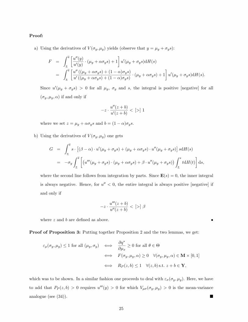
Proof:
a) Using the derivatives of V (σy, µy) yields (observe that y = µy + σys):
F =∫ s
s
[u′′(y)u′(y)
· (µy + ασys) + 1]
u′(µy + σys)dH(s)
=∫ s
s
[u′′ ((µy + ασys) + (1− α)σys)u′ ((µy + ασys) + (1− α)σys)
· (µy + ασys) + 1]
u′(µy + σys)dH(s).
Since u′(µy + σys) > 0 for all µy, σy and s, the integral is positive [negative] for all
(σy, µy, α) if and only if
−z · u′′(z + b)u′(z + b)
< [>] 1
where we set z = µy + ασys and b = (1− α)σys.
b) Using the derivatives of V (σy, µy) one gets
G =∫ s
ss ·
[(β − α) · u′(µy + σys) + (µy + ασys) · u′′(µy + σys)
]sdH(s)
= −σy
∫ s
s
[(u′′′(µy + σys) · (µy + ασys) + β · u′′(µy + σys)
) ∫ s
stdH(t)
]ds,
where the second line follows from integration by parts. Since E(s) = 0, the inner integral
is always negative. Hence, for u′′ < 0, the entire integral is always positive [negative] if
and only if
−z · u′′′(z + b)u′′(z + b)
< [>] β
where z and b are defined as above. •
Proof of Proposition 3: Putting together Proposition 2 and the two lemmas, we get:
εµ(σy, µy) ≤ 1 for all (µy, σy) ⇐⇒ ∂q∗
∂µx≥ 0 for all θ ∈ Θ
⇐⇒ F (σy, µy, α) ≥ 0 ∀(σy, µy, α) ∈ M× [0, 1]
⇐⇒ RP (z, b) ≤ 1 ∀(z, b) s.t. z + b ∈ Y,
which was to be shown. In a similar fashion one proceeds to deal with εσ(σy, µy). Here, we have
to add that PP (z, b) > 0 requires u′′′(y) > 0 for which Vµσ(σy, µy) > 0 is the mean-variance
analogue (see (34)). �
25
References
Arrondel, L., and H. Calvo-Pardo, 2002, Portfolio choice with a correlated background risk:
Theory and evidence. DELTA Working Papers 2002-16, DELTA (Ecole Nationale Superiore),
Paris.
Bigelow, J.P., 1993, Consistency of mean-variance analysis and expected utility analysis. Eco-
nomics Letters 43, 187-192.
Bigelow, J.P., and C.F. Menezes, 1995, Outside risk aversion and the comparative statics of
increasing risk in quasi-linear decision models. International Economic Review 36, 643–673.
Chamberlain, G., 1983, A characterization of the distributions that imply mean-variance utility
functions. Journal of Economic Theory 29, 185–201.
Cheng, H.-C., M. J. Magill and W. J. Shafer, 1987, Some results on comparative statics under
uncertainty. International Economic Review 28, 493–507.
Chipman, J. S., 1973, The ordering of portfolios in terms of mean and variance. Review of
Economic Studies 40, 167–190.
Diamond, P., and J.E. Stiglitz, 1974, Increases in risk and risk aversion. Journal of Economic
Theory 8, 337–360.
Dionne, G., L. Eeckhoudt, and C. Gollier, 1993, Increases in risk and linear payoffs. International
Economic Review 34, 309–319.
Eeckhoudt, L., C. Gollier, and H. Schlesinger, 1996, Changes in background risk and risk taking
behaviour. Econometrica 64, 683–689.
Eichner, T., 2005, Comparative statics of properness in two-moment decision models. Economic
Theory 25, 1007–1012.
Eichner, T. 2007, Mean-variance vulnerability. Management Science, forthcoming.
Eichner, T., and A. Wagener, 2003a, Variance vulnerability, background risks, and mean variance
preferences. The Geneva Papers on Risk and Insurance Theory 28, 173-184.
26
Eichner, T., and A. Wagener, 2003b, More on parametric characterizations of risk aversion and
prudence. Economic Theory 21, 895-900.
Elmendorff, D.W., and M.S. Kimball, 2000, Taxation of labor income and the demand for risky
assets. International Economic Review 41, 801-832.
Embrechts, P., A. McNeil, and D. Straumann, 2002, Correlation and dependence in risk man-
agement: Properties and pitfalls. In: Dempster, M.A.H. (ed.), Risk Management: Value at
Risk and Beyond, Cambridge University Press, Cambridge, pp. 176-223.
Fang, K.-T., S. Kotz, and K.-W. Ng, 1990, Symmetric Multivariate and Related Distributions,
Chapman and Hall: London/New York.
Feder, G., 1977, The impact of uncertainty in a class of objective functions. Journal of Economic
Theory 16, 504–512.
Fishburn, P.C., and R.B. Porter, 1976, Optimal portfolios with one safe and one risky asset:
Effects of changes in rate of return and risk. Management Science 22, 1064–1073.
Gollier, C., and J. W. Pratt, 1996, Risk vulnerability and the tempering effect of background
risk. Econometrica 64, 1109–1123.
Hadar, J., and T. Seo, 1992, A note on beneficial changes in random variables. The Geneva
Papers on Risk and Insurance Theory 17, 171–179.
Hanson, D. L. and C. F. Menezes, 1968, Risk aversion and bidding theory. In: Quirk, J. P. and
A. M. Zarley, eds., Papers in Quantitative Economics, Vol. 1 (Lawrence etc.: The University
Press of Kansas), 521–542.
Hawawini, G. A., 1978, A mean-standard deviation exposition of the theory of the firm under
uncertainty. A pedagogical note. American Economic Review 68, 194–202.
Kimball, M. S., 1993, Standard risk aversion. Econometrica 61, 589–611.
Lajeri, F., 1995, Further results on risk aversion and prudence: the case of independent risks.
Unpublished INSEAD Dissertation.
27
Lajeri-Chaherli, F., 2002, More on properness: the case of mean-variance preferences. The
Geneva Papers on Risk and Insurance Theory 27, 49–60.
Lajeri-Chaherli, F., 2003, Partial derivatives, comparative risk behavior and concavity of utility
functions. Mathematical Social Sciences 46, 81–89.
Lajeri-Chaherli, F., 2005, Proper and standard risk aversion in two-moment decision models.
Theory and Decision 57, 213–225.
Lajeri, F., and L.T. Nielsen, 1995, Risk aversion and prudence: the case of mean-variance
preferences, INSEAD working paper.
Lajeri, F., and L. T. Nielsen, 2000, Parametric characterizations of risk aversion and prudence.
Economic Theory 15, 469–476.
Markowitz, H., 1952, Portfolio selection. Journal of Finance 7, 77-91.
Markowitz, H., 1999, The early history of portfolio theory: 1600-1960. Financial Analysts Jour-
nal 55, 5-16.
Mathews, T., 2004, Meaning of ‘more risk averse’ when preferences are over mean and variance.
The Manchester School 73, 75–91.
Meyer, J., 1987, Two-moment decision models and expected utility maximization. American
Economic Review 77, 421–430.
Meyer, J., 1992, Beneficial changes in random variables under multiple sources of risk and their
comparative statics. The Geneva Papers on Risk and Insurance Theory 17, 7–19.
Ormiston, M. B., and E. E. Schlee, 2001, Mean-variance preferences and investor behaviour.
The Economic Journal 111, 849–861.
Owen, J., and R. Rabinovitch, 1983, On the class of elliptical distributions and their applications
to the theory of portfolio choice. Journal of Finance 38, 745–752.
Pratt, J.W., 1964, Risk aversion in the small and in the large. Econometrica 32, 122–136.
Pratt, J.W., and R.J. Zeckhauser, 1987, Proper risk aversion. Econometrica 55, 143–154.
28
Ross, S.A., 1981, Some stronger measures of risk aversion in the small and in the large with
applications. Econometrica 49, 621–638.
Saha, A. (1997): Risk preference estimation in the non-linear standard deviation approach.
Economic Inquiry 35, 770–782.
Sandmo, A., 1971, On the theory of the competitive firm under price uncertainty. American
Economic Review 61, 65–73.
Sinn, H.-W., 1983, Economic Decisions under Uncertainty. North-Holland: Amsterdam.
Tobin, J., 1958, Liquidity preference as behaviour towards risk. Review of Economic Studies 67,
65–86.
Tibiletti, L., 1995, Beneficial changes in random variables via copulas: An application to insur-
ance. Geneva Papers on Risk and Insurance Theory 20, 191-202.
Wagener, A., 2002, Prudence and risk vulnerability in two-moment decision models. Economics
Letters 74, 229–235.
Wagener, A., 2005, Linear risk tolerance and mean-variance preferences. Economics Bulletin 4,
1-8.
29