Embed Size (px)
Citation preview
CRANFIELD UNIVERSITY
Anayo Isaac Ogazi
Multiphase Severe Slug Flow
Control
School of Engineering
Process Systems Group
PhD Thesis

CRANFIELD UNIVERSITY
School of Engineering, Department of Offshore, Process and Energy
Engineering
Process Systems Group
PhD Thesis
Anayo Isaac Ogazi
Multiphase Severe Slug Flow Control
Dr. Yi Cao
Supervisor
January, 2011
This thesis is submitted in fulfilment of the requirements for the degree of
Doctor of Philosophy
c© Cranfield University 2011. All rights reserved. No part of this publication may be
reproduced without the written permission of the copyright holder.


This thesis is dedicated to the memory of my mother Mrs Maria Ogazi,
whose love and sacrifices laid the foundation for these achievements.

Abstract
Severe slug flow is one of the most undesired multiphase flow regimes, due
to the associated instability, which imposes major challenges to flow assurance
in the oil and gas industry. This thesis presents a comprehensive analysis of
the systematic approach to achieving stability and maximum production from an
unstable riser-pipeline system. The development of a plant-wide model which
comprises an improved simplified riser model (ISRM) required for severe slug
controller design and control performance analysis is achieved. The ability of
the ISRM to predict nonlinear stability of the unstable riser-pipeline is investi-
gated using an industrial riser and a 4 inch laboratory riser system. Its predic-
tion of the nonlinear stability showed close agreement with experimental and
simulation results.
Through controllability analysis of the unstable riser-pipeline system, which
is focused on achieving the core operational targets of the riser-pipeline produc-
tion system, the maximum stable valve opening achievable with each controlled
variable considered is predicted and confirmed through the simulation results.
The potential to increase oil production through feedback control is presented
by analysing the pressure production relationship using a pressure dependent
dimensionless variable known as Production Gain Index (PGI).
The performance analyses of three active slug controllers are presented to
show that the ability of a slug controller to achieve closed loop stability at large
valve opening can be assessed by the analysis of the H∞ norm of the comple-
mentary sensitivity function of the closed loop system, ‖T (s)‖∞. A slug con-
troller which achieves the lowest value of the ‖T (s)‖∞, will achieve closed loop
stability at a larger valve opening. Finally, the development of a new improved
relay auto-tuned slug controller algorithm based on a perturbed first-order-plus
dead-time (FOPDT) model of the riser system is achieved. Its performance
showed that it has the ability to stabilise the riser system at a valve opening
that is larger than that achieved with the original (conventional) algorithm with
about 4% increase in production.
VIII

Acknowledgements
It is with great pleasure and thanks to the Almighty God that I write this
section to acknowledge many individuals and organisations who have sown
their golden treasures, talent and time into me and into this work to make it a
success.
Firstly, without any iota of reservation, I am saying a very loud thank you
to my able and understanding supervisor, Dr. Yi Cao, whose guidance and
encouragement was pivotal to the success of this work. His style of leading
the way and at the same time allowing you to lead, made a lot of difference
in building my research skills and completing this work. I will not fail to also
thank the head of the Process Systems Engineering Group, Prof. Hoi Yeung,
whose wealth of experience advice meant a lot to the success of this work.
Thank you Prof. Hoi. The entire Process Systems Engineering Group team
has been exceptionally fantastic. The likes of Sam Skears (the administrator)
whose support and advice was always there will always be appreciated by me.
I will not forget to thank the Multiphase flow laboratory technicians, David and
Clerve for their support during my experiment periods in the laboratory.
It is important to stress that this work has been undertaken within the Joint
Project on Transient Multiphase Flows and Flow Assurance. I wish to acknowl-
edge the contributions made to this project by the UK Engineering and Physical
Sciences Research Council (EPSRC) and the following: - Advantica; BP Explo-
ration; CD-adapco; Chevron; ConocoPhillips; ENI; ExxonMobil; FEESA; IFP;
Institutt for Energiteknikk; PDVSA (INTEVEP); Petrobras; PETRONAS; Scand-

power PT; Shell; SINTEF; StatoilHydro and TOTAL. I wish to express my sin-
cere gratitude for this support. I also wish to thank SPT Group Ltd for the use of
OLGA during this work and for providing an OLGA model of a tie-back system
for use in testing the slug control algorithm. OLGA is a registered trademark of
SPT Group.
I will like to thank my friends and colleagues in Cranfield University, including
Dr. Ogaji Stephen, Dr. Gareth Davis, Tesi Arubi, Ade Lawal, Daniel Kamunge,
Patricia Odiowei, Edith Ejikeme and Lanchang. Special thanks to my brother
and friend Crispin Alison for his soul motivation and encouragement especially
when the going gets though. Thank you all.
With heart full of thanks, I wish to say to the entire Holding Forth the Word
Ministry including the Cranfield Pentecostal Assembly that you have given me
what money cannot buy, the eternal peace and family to succeed. The heart of
love of Pastor Biyi Ajala will always be in my memory.
My entire family has always been there for me in full measure. The love and
sacrifice of my wife, Mrs Tina Nkiruka Ogazi and my little daughter Miss Bithiah
Chimnechem Ogazi will always be appreciated. The support and prayers of my
brother Elder Emeka Ogazi and his family and special cousin Mrs Ede Nwali
Elizabeth and her family will always be in my heart. Obviously, words and
space may have failed me in expressing my deep held appreciation to many
who should be on this page, but in my heart, that which words cannot say is
written. Thank you.
X
Contents
Abstract VII
Acknowledgements IX
Notation XXVII
1 Introduction 1
1.1 Background and motivation . . . . . . . . . . . . . . . . . . . . . 1
1.1.1 The riser-pipeline system . . . . . . . . . . . . . . . . . . 2
1.1.2 Severe slugging phenomenon . . . . . . . . . . . . . . . 3
1.1.2.1 Typical severe slug profile . . . . . . . . . . . . . 4
1.2 Project aim and objectives . . . . . . . . . . . . . . . . . . . . . . 6
1.3 Methodology . . . . . . . . . . . . . . . . . . . . . . . . . . . . . 7
1.4 Thesis outline and contributions . . . . . . . . . . . . . . . . . . . 9
1.5 Publications . . . . . . . . . . . . . . . . . . . . . . . . . . . . . . 12
1.5.1 Conference papers . . . . . . . . . . . . . . . . . . . . . . 12
1.5.2 Journal paper . . . . . . . . . . . . . . . . . . . . . . . . . 13
2 Literature review 15
2.1 Introduction . . . . . . . . . . . . . . . . . . . . . . . . . . . . . . 15
2.2 Multiphase flow . . . . . . . . . . . . . . . . . . . . . . . . . . . . 15
2.2.1 Multiphase flow regimes . . . . . . . . . . . . . . . . . . . 16
XI
2.2.1.1 Multiphase two-phase gas-liquid flow regimes in
horizontal pipe . . . . . . . . . . . . . . . . . . . 17
2.2.1.2 Multiphase two-phase flow regimes in vertical pipe 20
2.3 Multiphase slug Flow . . . . . . . . . . . . . . . . . . . . . . . . . 22
2.3.1 Hydrodynamic slugging . . . . . . . . . . . . . . . . . . . 22
2.3.2 Operation induced slug . . . . . . . . . . . . . . . . . . . 23
2.3.3 Severe slugging . . . . . . . . . . . . . . . . . . . . . . . 24
2.3.3.1 Severe slug models . . . . . . . . . . . . . . . . 24
2.4 Severe slugging control techniques and technologies . . . . . . . 29
2.4.1 Changing flow condition . . . . . . . . . . . . . . . . . . . 30
2.4.1.1 Design modification of upstream facilities . . . . 30
2.4.1.2 Riser base gas lift . . . . . . . . . . . . . . . . . 32
2.4.1.3 Gas re-injection . . . . . . . . . . . . . . . . . . 35
2.4.1.4 Homogenising the multiphase flow . . . . . . . . 37
2.4.1.5 Sub-sea separation of multiphase fluid . . . . . 37
2.4.2 Riser outlet downstream adjustment . . . . . . . . . . . . 38
2.4.2.1 Design modification of processing facilities . . . 38
2.4.2.2 Topside choke control . . . . . . . . . . . . . . . 39
2.5 Conclusions . . . . . . . . . . . . . . . . . . . . . . . . . . . . . . 47
3 Experimental facilities and procedure 49
3.1 Introduction . . . . . . . . . . . . . . . . . . . . . . . . . . . . . . 49
3.2 The multiphase flow facility . . . . . . . . . . . . . . . . . . . . . 50
3.2.1 Fluid supply and metering section . . . . . . . . . . . . . 50
3.2.1.1 Air supply . . . . . . . . . . . . . . . . . . . . . . 52
3.2.1.2 Water and oil supply . . . . . . . . . . . . . . . . 52
3.2.1.3 Flow metering . . . . . . . . . . . . . . . . . . . 53
3.2.2 The test section . . . . . . . . . . . . . . . . . . . . . . . 54
3.2.2.1 The 4 inch riser system . . . . . . . . . . . . . . 54
XII
3.2.2.2 The 2 inch riser system . . . . . . . . . . . . . . 55
3.2.2.3 Two-phase separator . . . . . . . . . . . . . . . 55
3.2.3 Phase separation section . . . . . . . . . . . . . . . . . . 57
3.2.3.1 The three-phase separator . . . . . . . . . . . . 57
3.3 Running the experiments . . . . . . . . . . . . . . . . . . . . . . 58
3.3.1 Operating condition . . . . . . . . . . . . . . . . . . . . . 58
3.4 Data acquisition system . . . . . . . . . . . . . . . . . . . . . . . 59
3.5 Industrial riser system . . . . . . . . . . . . . . . . . . . . . . . . 59
3.6 Flow rate and operating conditions . . . . . . . . . . . . . . . . . 60
4 Plant-wide modeling for severe slugging prediction and control 61
4.1 Introduction . . . . . . . . . . . . . . . . . . . . . . . . . . . . . . 61
4.2 Plant-wide model . . . . . . . . . . . . . . . . . . . . . . . . . . . 62
4.2.1 The riser-pipeline model . . . . . . . . . . . . . . . . . . . 62
4.2.1.1 Suitability of riser-pipeline models . . . . . . . . 63
4.2.1.2 Simplified riser model (SRM) . . . . . . . . . . . 64
4.3 Improved simplified riser model (ISRM) . . . . . . . . . . . . . . 67
4.3.1 Conservation equations of the ISRM . . . . . . . . . . . . 68
4.3.1.1 Dynamic riser outlet boundary condition - the
separator model . . . . . . . . . . . . . . . . . . 69
4.3.2 State dependent variables . . . . . . . . . . . . . . . . . . 72
4.3.2.1 Dynamic update of upstream gas volume . . . . 73
4.3.2.2 Gas volume at the riser top . . . . . . . . . . . . 74
4.3.2.3 Internal gas flow rate . . . . . . . . . . . . . . . 74
4.3.3 Entrainment equation . . . . . . . . . . . . . . . . . . . . 75
4.3.3.1 Prediction of the slug production stage . . . . . 75
4.3.4 Fluid flow out of the riser . . . . . . . . . . . . . . . . . . . 78
4.3.4.1 Pressure driven fluid source . . . . . . . . . . . 78
4.3.5 ISRM and SRM tuning parameters . . . . . . . . . . . . . 81
XIII
4.3.6 Performances of the ISRM with separator model . . . . . 82
4.3.6.1 Prediction of severe slugging flow with variable
fluid inlet flow rate . . . . . . . . . . . . . . . . . 83
4.3.6.2 Prediction of severe slug frequency and pres-
sure amplitude . . . . . . . . . . . . . . . . . . . 84
4.3.6.3 Prediction of the slug production stage . . . . . 86
4.3.6.4 Prediction of flow regime map . . . . . . . . . . 88
4.4 Model nonlinear stability analyses . . . . . . . . . . . . . . . . . 90
4.4.1 Open-loop root locus . . . . . . . . . . . . . . . . . . . . . 90
4.4.2 Hopf bifurcation map . . . . . . . . . . . . . . . . . . . . . 91
4.4.3 Nonlinear stability analyses of the industrial riser system . 92
4.4.3.1 Open-loop root locus plot of the industrial riser
system . . . . . . . . . . . . . . . . . . . . . . . 92
4.4.3.2 Hopf bifurcation of the industrial riser system . . 93
4.4.4 Nonlinear stability analyses of the 4 inch riser system . . 94
4.4.4.1 Open-loop root locus plot of the 4 inch riser sys-
tem . . . . . . . . . . . . . . . . . . . . . . . . . 94
4.4.4.2 Hopf Bifurcation of the 4 inch riser system . . . 95
4.5 Conclusions . . . . . . . . . . . . . . . . . . . . . . . . . . . . . . 96
5 Controllability analysis of unstable riser-pipeline system 99
5.1 Introduction . . . . . . . . . . . . . . . . . . . . . . . . . . . . . . 99
5.1.1 Limitations of the riser-pipeline controllability analysis . . 101
5.2 Controllability analysis tools . . . . . . . . . . . . . . . . . . . . . 103
5.2.1 Control objectives . . . . . . . . . . . . . . . . . . . . . . 103
5.2.2 Valve opening and production . . . . . . . . . . . . . . . . 104
5.2.3 Lower bound on the input magnitude . . . . . . . . . . . . 105
5.2.4 Scaling . . . . . . . . . . . . . . . . . . . . . . . . . . . . 106
5.2.5 Linear model transfer functions . . . . . . . . . . . . . . . 107
XIV
5.2.5.1 Deriving the nonlinear functions . . . . . . . . . 108
5.3 Controllability analysis with the riser top valve opening, u . . . . 111
5.3.1 Lower bound on KS analysis . . . . . . . . . . . . . . . . 113
5.4 Controllability analysis with the topside separator gas valve ug . . 117
5.4.1 Nonlinear stability analysis . . . . . . . . . . . . . . . . . 118
5.4.1.1 Open-loop root locus plot . . . . . . . . . . . . . 118
5.4.1.2 Hopf bifurcation map . . . . . . . . . . . . . . . 119
5.4.2 Linear model transfer functions . . . . . . . . . . . . . . . 120
5.4.3 Lower bound on KS analysis . . . . . . . . . . . . . . . . 122
5.5 Simulations and results analyses . . . . . . . . . . . . . . . . . . 125
5.5.1 The simulation model . . . . . . . . . . . . . . . . . . . . 125
5.5.2 Control structure with derivative controller . . . . . . . . . 126
5.5.2.1 Routh stability criterion . . . . . . . . . . . . . . 128
5.5.3 Simulation with riser top valve (u) as manipulated variable 129
5.5.3.1 Simulation procedure . . . . . . . . . . . . . . . 129
5.5.3.2 PRB control . . . . . . . . . . . . . . . . . . . . . 130
5.5.3.3 PRT control . . . . . . . . . . . . . . . . . . . . . 135
5.5.3.4 QT control . . . . . . . . . . . . . . . . . . . . . 138
5.5.3.5 Analyses and comparison of simulated results . 139
5.5.4 Simulation with topside separator gas valve (ug) as ma-
nipulated variable . . . . . . . . . . . . . . . . . . . . . . 141
5.5.5 Simulation results analyses and comparison . . . . . . . 143
5.6 Comparison of the controllability with u and ug . . . . . . . . . . . 147
5.7 Conclusions . . . . . . . . . . . . . . . . . . . . . . . . . . . . . . 148
6 Production potential of severe slug control system 151
6.1 Introduction . . . . . . . . . . . . . . . . . . . . . . . . . . . . . . 151
6.2 Pressure and production . . . . . . . . . . . . . . . . . . . . . . . 152
6.2.1 Linear well productivity . . . . . . . . . . . . . . . . . . . . 153
XV
6.2.2 Unstable systems . . . . . . . . . . . . . . . . . . . . . . 154
6.2.3 Stable systems . . . . . . . . . . . . . . . . . . . . . . . . 155
6.3 Production Gain Index (PGI) . . . . . . . . . . . . . . . . . . . . . 156
6.4 Case study - the industrial riser system . . . . . . . . . . . . . . 157
6.4.1 The PWH and the PWHc for the industrial riser system . . 158
6.4.1.1 Calculating the PWH . . . . . . . . . . . . . . . . 158
6.4.1.2 Calculating the PWHc . . . . . . . . . . . . . . . 159
6.4.2 PGI analysis . . . . . . . . . . . . . . . . . . . . . . . . . 161
6.4.3 Simulated production . . . . . . . . . . . . . . . . . . . . 163
6.4.3.1 The simulation model and controller . . . . . . . 163
6.4.3.2 Implementation of the relay tuned slug controller 164
6.4.3.3 Implementation of the robust PID slug controller 165
6.4.4 Simulated production comparison . . . . . . . . . . . . . 166
6.4.5 PGI analysis for different reservoir pressures . . . . . . . 167
6.5 Conclusions . . . . . . . . . . . . . . . . . . . . . . . . . . . . . . 169
7 Design and characterisation of slug controllers for maximising oil
production 171
7.1 Introduction . . . . . . . . . . . . . . . . . . . . . . . . . . . . . . 171
7.2 Characterisation of slug controllers . . . . . . . . . . . . . . . . . 173
7.3 Slug controller design techniques . . . . . . . . . . . . . . . . . . 176
7.3.1 Relay auto-tuned slug controller . . . . . . . . . . . . . . 176
7.3.1.1 Process identification using relay feedback shape
factor . . . . . . . . . . . . . . . . . . . . . . . . 178
7.3.1.2 Process and controller parameters . . . . . . . . 180
7.3.1.3 Relay auto-tuned controller design for PRB con-
trol of the 2 inch riser . . . . . . . . . . . . . . . 181
7.3.1.4 Relay auto-tuned slug controller design for an
industrial riser . . . . . . . . . . . . . . . . . . . 187
XVI
7.3.2 Robust PID slug controller . . . . . . . . . . . . . . . . . . 190
7.3.2.1 Controller design criteria . . . . . . . . . . . . . 191
7.3.2.2 Robust PID controller design for the industrial
riser system . . . . . . . . . . . . . . . . . . . . 193
7.3.3 H∞ robust slug controller . . . . . . . . . . . . . . . . . . 196
7.3.3.1 Control configuration . . . . . . . . . . . . . . . 196
7.3.3.2 Controller design criteria . . . . . . . . . . . . . 198
7.3.3.3 Un-modelled dynamic uncertainty . . . . . . . . 200
7.3.3.4 H∞ robust slug controller design for the indus-
trial riser . . . . . . . . . . . . . . . . . . . . . . 200
7.4 Characterisation of the slug controllers for closed-loop stability at
large valve opening . . . . . . . . . . . . . . . . . . . . . . . . . . 203
7.4.1 Characterisation of PRB controller . . . . . . . . . . . . . 204
7.4.2 Characterisation of QT controller . . . . . . . . . . . . . . 204
7.5 Slug controller implementation and simulated production analysis 205
7.5.1 Slug controller implementation with PRB control . . . . . . 206
7.5.1.1 Implementation of the relay auto-tuned slug con-
troller . . . . . . . . . . . . . . . . . . . . . . . . 206
7.5.1.2 Implementation of the robust PID slug controller 208
7.5.1.3 Implementation of H∞ robust slug controller . . 212
7.5.1.4 Comparison of maximum stable valve opening
and simulated production . . . . . . . . . . . . . 214
7.5.2 Stability and production in declining reservoir pressure
condition . . . . . . . . . . . . . . . . . . . . . . . . . . . 217
7.5.3 Slug controller implementation with QT control . . . . . . 219
7.6 Conclusions . . . . . . . . . . . . . . . . . . . . . . . . . . . . . . 222
8 Improved relay auto-tuned slug controller design for increased oil
production 225
XVII
8.1 Introduction . . . . . . . . . . . . . . . . . . . . . . . . . . . . . . 225
8.2 The perturbed (uncertain) FOPDT model . . . . . . . . . . . . . 226
8.3 Relay auto-tuned controller synthesis . . . . . . . . . . . . . . . . 229
8.4 Controller design and implementation . . . . . . . . . . . . . . . 232
8.4.1 Controller design and implementation with PRB control . . 232
8.4.1.1 Controller implementation . . . . . . . . . . . . . 235
8.4.2 Controller design and implementation with QT control . . 237
8.4.2.1 Controller implementation . . . . . . . . . . . . . 239
8.5 Control with topside separator gas valve, (ug) . . . . . . . . . . . 240
8.5.1 Control with the PRB . . . . . . . . . . . . . . . . . . . . . 241
8.6 Conclusions . . . . . . . . . . . . . . . . . . . . . . . . . . . . . . 245
9 Conclusions and further work 247
9.1 Conclusion . . . . . . . . . . . . . . . . . . . . . . . . . . . . . . 247
9.2 Future work . . . . . . . . . . . . . . . . . . . . . . . . . . . . . . 251
A Simplified riser model (SRM) equations 253
A.1 Conservation equations . . . . . . . . . . . . . . . . . . . . . . . 253
A.2 State dependent variables . . . . . . . . . . . . . . . . . . . . . . 254
A.3 Fluid flow equations . . . . . . . . . . . . . . . . . . . . . . . . . 255
A.4 Entrainment equation . . . . . . . . . . . . . . . . . . . . . . . . 256
B Nonlinear functions for evaluating system linear transfer functions257
B.1 Nonlinear functions for the PRB with u . . . . . . . . . . . . . . . 257
B.2 Nonlinear functions for the PRT with u . . . . . . . . . . . . . . . 258
B.3 Nonlinear functions for the QT with u . . . . . . . . . . . . . . . . 259
B.4 Nonlinear functions for the PRB with ug . . . . . . . . . . . . . . . 259
B.5 Nonlinear functions for the Ps with ug . . . . . . . . . . . . . . . . 260
B.6 Nonlinear functions for the PRT with ug . . . . . . . . . . . . . . . 261
XVIII
B.7 Nonlinear functions for the QGsep with ug . . . . . . . . . . . . . . 262
References 263
XIX

XX
List of Figures
1.1 Severe slug cycle phenomenon illustrated . . . . . . . . . . . . . 4
1.2 Typical severe slug flow profile . . . . . . . . . . . . . . . . . . . 5
1.3 Oscillatory slug flow profile . . . . . . . . . . . . . . . . . . . . . 6
2.1 Diagram showing hierarchy of literature review structure . . . . . 16
2.2 Two-phase gas-liquid flow regime, [107] . . . . . . . . . . . . . . 18
2.3 Hierarchial diagram showing flow regime in two-phase flow . . . 18
2.4 Flow pattern for two-phase gas-liquid flow, [114] . . . . . . . . . 19
2.5 Flow pattern for two-phase gas-liquid vertical flow, [38] . . . . . . 21
2.6 Stratified flow criterion [108] . . . . . . . . . . . . . . . . . . . . . 26
2.7 Device for slug inhibition, [63] . . . . . . . . . . . . . . . . . . . . 32
2.8 Multi-purpose riser for slug control [19] . . . . . . . . . . . . . . . 34
2.9 Gas re-injection system for riser slug control, [110] . . . . . . . . 35
2.10 Gas by-pass method . . . . . . . . . . . . . . . . . . . . . . . . . 36
2.11 Schematic diagram of a horizontal slug catcher . . . . . . . . . . 39
2.12 Schematic diagram of the ABB SlugCon Control System, [40] . . 43
2.13 Cascade control configuration for severe slug control . . . . . . . 44
2.14 Schematic diagram of the S3 control scheme . . . . . . . . . . . 45
2.15 Schematic diagram of the slug mitigation system, [78] . . . . . . 46
3.1 Multiphase facility at Cranfield University . . . . . . . . . . . . . . 51
3.2 Water and oil pumps . . . . . . . . . . . . . . . . . . . . . . . . . 53
3.3 Two phase separator picture at the test section . . . . . . . . . . 56
XXI
3.4 Schematic diagram of the industrial riser-pipeline system . . . . 60
4.1 Riser-pipeline schematic diagram for the SRM . . . . . . . . . . 64
4.2 Riser-pipeline schematic diagram for the ISRM . . . . . . . . . . 67
4.3 Two phase separator diagram . . . . . . . . . . . . . . . . . . . . 70
4.4 Riser base pressure from experiment . . . . . . . . . . . . . . . 77
4.5 Model tuning flow chart . . . . . . . . . . . . . . . . . . . . . . . 81
4.6 Comparison of SRM and ISRM with the experimental result . . . 83
4.7 Riser base pressure from experiment . . . . . . . . . . . . . . . 84
4.8 Riser base pressure of SRM with amplitude fitted . . . . . . . . . 85
4.9 Riser base pressure of SRM with frequency fitted . . . . . . . . . 85
4.10 Riser base pressure of ISRM with amplitude and frequency fitted 85
4.11 Typical severe slug profile . . . . . . . . . . . . . . . . . . . . . . 87
4.12 PRB profile under severe slugging condition, experimental result 87
4.13 PRB profile under severe slugging condition, ISRM . . . . . . . . 88
4.14 PRB profile under severe slugging condition, SRM . . . . . . . . 88
4.15 Flow regime map of 4 inch catenary riser . . . . . . . . . . . . . 89
4.16 Riser pipeline system with u and ug . . . . . . . . . . . . . . . . . 90
4.17 Open-loop root locus for the industrial riser system . . . . . . . . 93
4.18 PRB bifurcation map of the industrial riser system . . . . . . . . . 93
4.19 Open-loop root locus for the 4 inch riser system . . . . . . . . . . 95
4.20 Pressure bifurcation map of the 4 inch riser system . . . . . . . . 96
5.1 Feedback control structure with set point . . . . . . . . . . . . . 101
5.2 Riser pipeline system with u and ug . . . . . . . . . . . . . . . . . 111
5.3 Riser base pressure Hopf bifurcation map . . . . . . . . . . . . . 114
5.4 Open-loop root locus plot with ug . . . . . . . . . . . . . . . . . . 118
5.5 Hopf bifurcation map . . . . . . . . . . . . . . . . . . . . . . . . . 120
5.6 Feedback control structure with set point equal to zero . . . . . . 127
XXII
5.7 Simulation result for the PRB . . . . . . . . . . . . . . . . . . . . . 134
5.8 Simulation result for the PRT . . . . . . . . . . . . . . . . . . . . . 137
5.9 Simulation result for the QT . . . . . . . . . . . . . . . . . . . . . 140
5.10 Simulation result with the PRB . . . . . . . . . . . . . . . . . . . . 144
5.11 Simulation result with the Ps . . . . . . . . . . . . . . . . . . . . . 144
5.12 Simulation result with the PRT . . . . . . . . . . . . . . . . . . . . 145
5.13 Simulation result with the QGouts . . . . . . . . . . . . . . . . . . . 145
6.1 Irregular dome slug profile . . . . . . . . . . . . . . . . . . . . . . 155
6.2 Well-head pressure profile . . . . . . . . . . . . . . . . . . . . . . 159
6.3 Well-head pressure Hopf bifurcation map of the industrial riser
system with PWH and PWHc . . . . . . . . . . . . . . . . . . . . . 160
6.4 Plot of the ZPGI for the industrial riser system . . . . . . . . . . . 161
6.5 Accumulated production, with and without relay tuned controller . 165
6.6 Accumulated production, with and without robust PID controller . 166
6.7 ZPGI line plot for different reservoir pressures . . . . . . . . . . . 168
7.1 Schematic diagram of the industrial riser-pipeline system . . . . 173
7.2 Detailed block diagram of a generalised control system . . . . . 174
7.3 Relay auto-tuning feedback control structure . . . . . . . . . . . 177
7.4 Relay test feedback response . . . . . . . . . . . . . . . . . . . . 178
7.5 Riser base pressure bifurcation map of the 2 inch riser . . . . . . 182
7.6 Relay feedback response of the 2 inch riser (Experimental result) 183
7.7 Relay feedback response of the 2 inch riser using the SRM . . . 183
7.8 Relay feedback response of the 2 inch riser using the ISRM . . . 184
7.9 Relay tuned controller implementation (Experimental result) . . . 185
7.10 Relay tuned controller implementation on the ISRM . . . . . . . . 186
7.11 Relay feedback response for PRB control . . . . . . . . . . . . . . 188
7.12 Relay feedback response for QT control . . . . . . . . . . . . . . 189
XXIII

7.13 Feedback control loop diagram for severe slug control . . . . . . 191
7.14 Generalised control system (GCS) diagram . . . . . . . . . . . . 197
7.15 Slug control with relay tuned controller . . . . . . . . . . . . . . . 207
7.16 Accumulated oil flow at different operating condition . . . . . . . 208
7.17 Slug control with robust PID controller - OLGA simulation . . . . 209
7.18 Slug control with robust PID controller - ISRM simulation . . . . . 209
7.19 Simulated production comparison I: severe slug production . . . 211
7.20 Simulated production comparison II: manual choking and no con-
trol . . . . . . . . . . . . . . . . . . . . . . . . . . . . . . . . . . . 212
7.21 Slug control with H-infinity controller . . . . . . . . . . . . . . . . 213
7.22 Accumulated oil at different operating points . . . . . . . . . . . . 214
7.23 Pressure bifurcation map showing controller’s maximum closed-
loop stable valve openings . . . . . . . . . . . . . . . . . . . . . . 215
7.24 Accumulated oil per day using each controller . . . . . . . . . . . 216
7.25 Stability at declining well pressure . . . . . . . . . . . . . . . . . 218
7.26 Percentage of production increase against well pressure . . . . . 219
7.27 Simulation result of the relay tuned slug controller . . . . . . . . . 220
7.28 Simulation result of the robust PID slug controller . . . . . . . . . 221
7.29 Simulation result of the H∞ robust slug controller . . . . . . . . . 221
8.1 Block diagram for controller synthesis . . . . . . . . . . . . . . . 229
8.2 Error and uncertainty weight plot . . . . . . . . . . . . . . . . . . 234
8.3 OLGA model simulation result with improved relay auto-tuned
controller . . . . . . . . . . . . . . . . . . . . . . . . . . . . . . . 235
8.4 Error and uncertainty weight plot . . . . . . . . . . . . . . . . . . 238
8.5 OLGA model simulation result with improved relay auto-tuned
controller . . . . . . . . . . . . . . . . . . . . . . . . . . . . . . . 239
8.6 Schematic diagram of the industrial riser-pipeline system . . . . 241
8.7 Relay feedback response for PRB control with ug . . . . . . . . . 242
XXIV
8.8 Simulation result for PRB control with ug . . . . . . . . . . . . . . 243
8.9 Improved relay controller simulation result for PRB control with ug 244
XXV

Notation
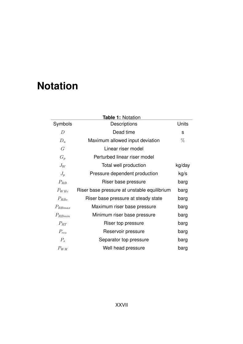
Table 1: NotationSymbols Descriptions Units
D Dead time s
Du Maximum allowed input deviation %
G Linear riser model
Gp Perturbed linear riser model
JW Total well production kg/day
Jp Pressure dependent production kg/s
PRB Riser base pressure barg
PWHc Riser base pressure at unstable equilibrium barg
PRBe Riser base pressure at steady state barg
PRBmax Maximum riser base pressure barg
PRBmin Minimum riser base pressure barg
PRT Riser top pressure barg
Pres Reservoir pressure barg
Ps Separator top pressure barg
PWH Well head pressure barg
XXVII
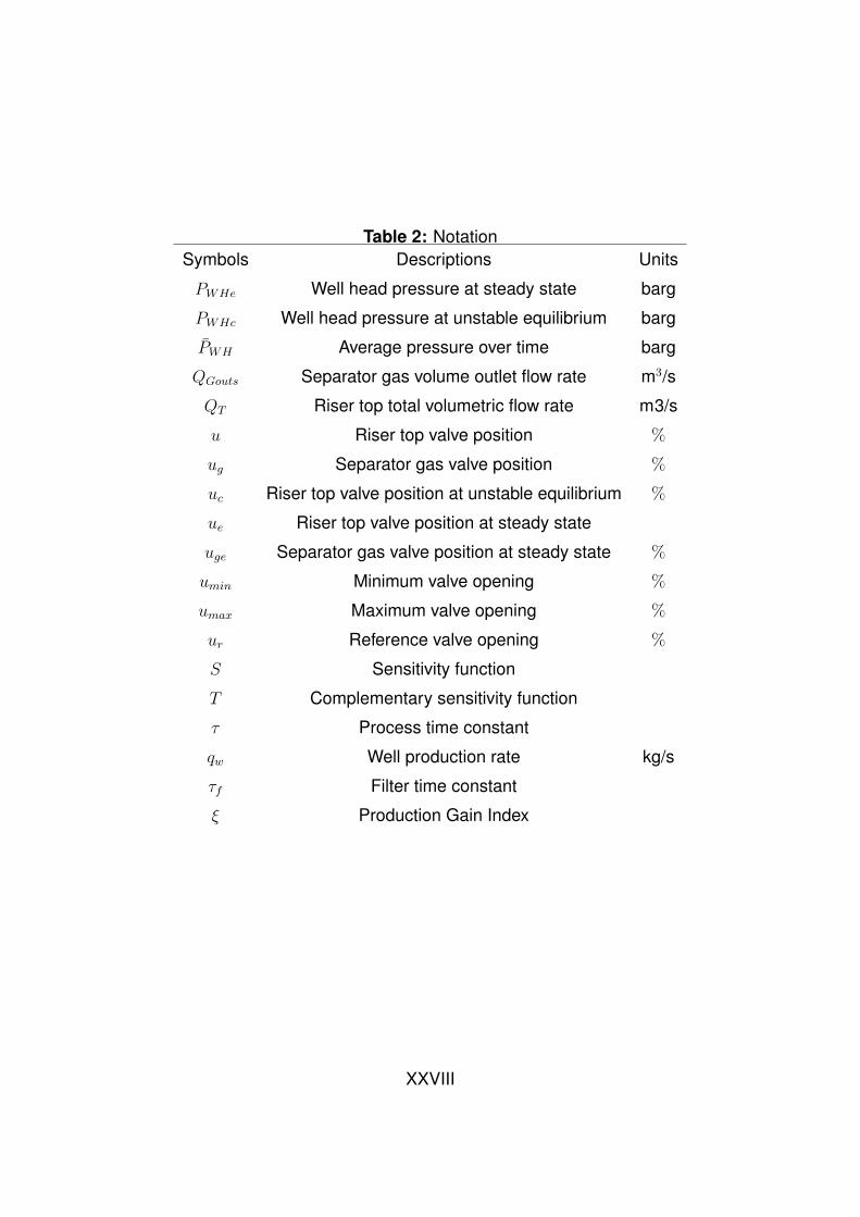
Table 2: NotationSymbols Descriptions Units
PWHe Well head pressure at steady state barg
PWHc Well head pressure at unstable equilibrium barg
PWH Average pressure over time barg
QGouts Separator gas volume outlet flow rate m3/s
QT Riser top total volumetric flow rate m3/s
u Riser top valve position %
ug Separator gas valve position %
uc Riser top valve position at unstable equilibrium %
ue Riser top valve position at steady state
uge Separator gas valve position at steady state %
umin Minimum valve opening %
umax Maximum valve opening %
ur Reference valve opening %
S Sensitivity function
T Complementary sensitivity function
τ Process time constant
qw Well production rate kg/s
τf Filter time constant
ξ Production Gain Index
XXVIII
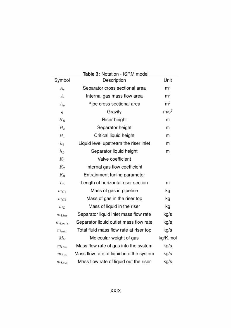
Table 3: Notation - ISRM modelSymbol Description Unit
As Separator cross sectional area m2
A Internal gas mass flow area m2
Ap Pipe cross sectional area m2
g Gravity m/s2
HR Riser height m
Hs Separator height m
H1 Critical liquid height m
h1 Liquid level upstream the riser inlet m
hL Separator liquid height m
K1 Valve coefficient
K2 Internal gas flow coefficient
K3 Entrainment tuning parameter
Lh Length of horizontal riser section m
mG1 Mass of gas in pipeline kg
mG2 Mass of gas in the riser top kg
mL Mass of liquid in the riser kg
mLins Separator liquid inlet mass flow rate kg/s
mLouts Separator liquid outlet mass flow rate kg/s
mmix Total fluid mass flow rate at riser top kg/s
MG Molecular weight of gas kg/K.mol
mGin Mass flow rate of gas into the system kg/s
mLin Mass flow rate of liquid into the system kg/s
mLout Mass flow rate of liquid out the riser kg/s
XXIX

Table 4: Notation - ISRM modelSymbol Description Unit
mGout Mass flow rate of gas out the riser kg/s
mG Internal gas mass flow rate kg/s
Ps Separator top pressure barg
PRB Riser base pressure barg
PRT Riser top pressure barg
QGins Separator gas volume inlet flow rate m3/s
QGouts Separator gas volume outlet flow rate m3/s
QT Total volumetric flowrate out of the riser m3/s
R Gas constant J/K/mol
T System temperature K
vG1 Internal gas velocity m/s
VG1 Volume of gas in the pipeline m3
VT Total riser volume m3
αLT liquid volume fraction at the riser top
αG Gas volume fraction in the pipeline
αmL Liquid mass fraction
ρG1 Pipeline gas density kg/m3
ρG2 Riser top gas density kg/m3
ρL Liquid density kg/m3
ρT Total fluid density at riser top kg/m3
u Riser top valve position %
XXX
Chapter 1
Introduction
1.1 Background and motivation
In the oil and gas production system, the ability to achieve continuous, safe,
economic and uninterrupted flow of oil and gas from the oil reservoir to the point
of sale is known as flow assurance. About 35% of the world energy supply is
from oil and gas. Recently, the rate of discovery of commercially viable oil fields
has been in serious decline, leading to increasing number of deep offshore
interests. The reservoir pressure in existing oil fields are known to decline
over time, making self lifting of oil to the topside difficult. In the North Sea oil
fields for example, production from existing oil fields have seen a decline of
about 11% since 1998 [84]. Despite these challenges, efforts are constantly
being made to ensure maximum oil recovery. In the drive to recover oil from
the reservoirs that are uneconomical to stand alone, production pipelines from
different oil fields could be tied in to one existing production platform, sometimes
resulting to long distant network of pipelines. Thus, the multiphase fluid has to
be transported through long distant horizontal pipelines and high risers, under
varying pressure, temperature and fluid composition condition.
1
2 Chapter 1. Introduction
With the complex nature of multiphase flow, these conditions can often gen-
erate some physical multiphase flow phenomena such as slug flow. Also,
physical-chemical phenomena such as wax deposition, emulsion, corrosion,
hydrates formation and sand deposition can be initiated in the pipeline. These
phenomena have the potential to obstruct the flow of oil and gas in the pipeline.
A competent flow assurance technology should be able to cover the whole
range of adequate understanding and knowledge, design tools as well as the
professional skills required to manage any form of these flow assurance prob-
lems. With the vast amount of work already put into developing these capabil-
ities, there are still wide gaps in the knowledge required to solve these whole
range of flow assurance problems.
The motivation for this research is to contribute to the adequate understanding
of the fundamental principles for eliminating a form of the slug flow, known as
severe slugging and at the same time maximise oil production. Severe slug-
ging is the most undesired flow regime in multiphase flow in the oil and gas
industry. It is characterised by intermittent flow of liquid and gas surges, which
impose significant challenges to the reservoir structure, the topside processing
efficiency and pipeline integrity.
1.1.1 The riser-pipeline system
The riser is a flow pipeline commonly applied in the oil and gas industry to
connect the horizontal upstream subsea pipes with the topside (downstream)
facilities. The primary function of the riser is to transport produced well fluid
(water, oil and gas) to the topside facilities for processing. Consequently, the
riser is positioned to connect the subsea pipelines at the sea bed to the topside
Chapter 1. Introduction 3
facilities. The riser height can vary from a few hundred metres to more than
2000 metres, depending on the sea bed depth from the topside. Also the riser
diameter can vary depending on the design it can also be designed into different
shapes, like the S-shaped riser.
1.1.2 Severe slugging phenomenon
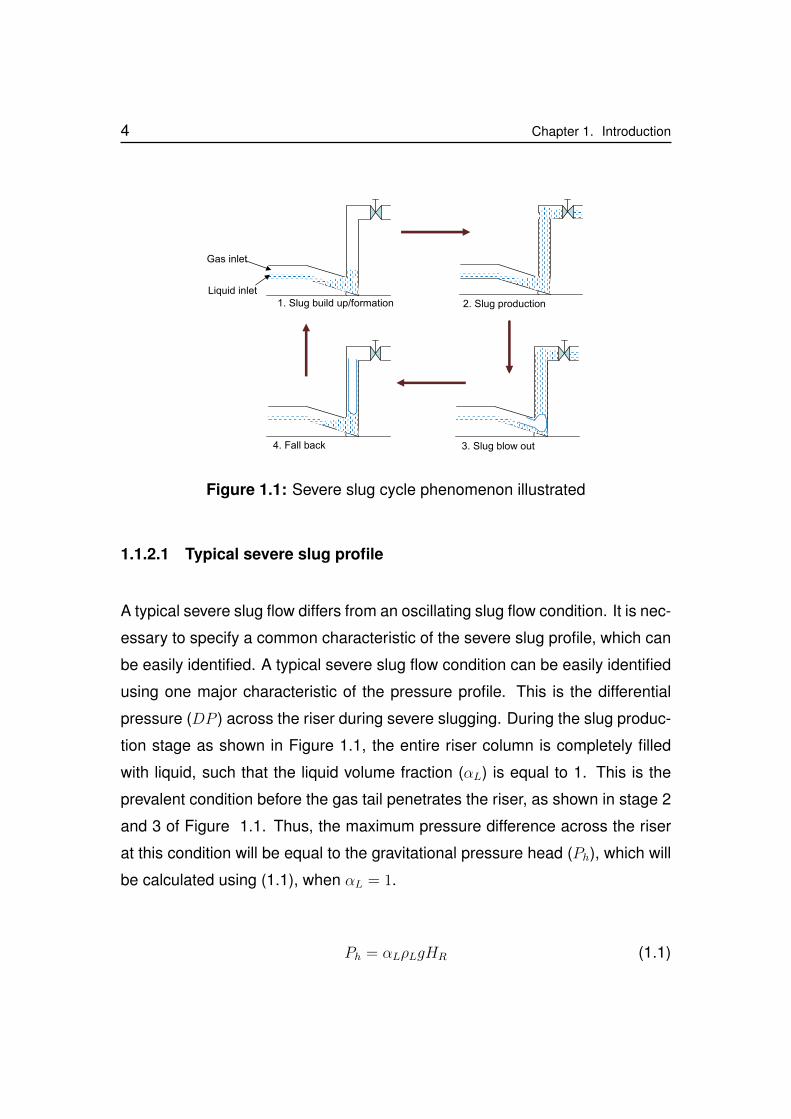
Severe slugging phenomenon is a four stage cyclic flow condition occurring in
the order as shown in Figure 1.1. One major condition for the occurrence of
severe slugging is the presence of dips and low points in the pipeline. This
causes liquid to accumulate at these dips, due to balance of pressure by op-
posing gravitational force. Thus, the liquid blocks the flowline (step 1). With
the flowline blocked, gas flow into the riser is stopped and further inlet gas is
compressed in the pipeline resulting in pipeline pressure build up, with a con-
tinuous liquid building up in the riser. This will continue until the pressure drop
across the riser overcomes the gravitational hydrostatic head in the riser; push-
ing the liquid slug out of the riser (step 2). This will result in a pressure drop in
the pipeline which allows the gas to expand, penetrate the liquid and increase
the flow velocity. With the gas tail entering the riser, the liquid is blown out
with a drop both in velocity and pressure (step 3). This causes the liquid to
fall back and block the riser base again (step 4). Detailed description of this
phenomenon can be found in the literature, e.g. [103]
4 Chapter 1. Introduction
Liquid inlet
Gas inlet
1. Slug build up/formation 2. Slug production
3. Slug blow out4. Fall back
Figure 1.1: Severe slug cycle phenomenon illustrated
1.1.2.1 Typical severe slug profile
A typical severe slug flow differs from an oscillating slug flow condition. It is nec-
essary to specify a common characteristic of the severe slug profile, which can
be easily identified. A typical severe slug flow condition can be easily identified
using one major characteristic of the pressure profile. This is the differential
pressure (DP ) across the riser during severe slugging. During the slug produc-
tion stage as shown in Figure 1.1, the entire riser column is completely filled
with liquid, such that the liquid volume fraction (αL) is equal to 1. This is the
prevalent condition before the gas tail penetrates the riser, as shown in stage 2
and 3 of Figure 1.1. Thus, the maximum pressure difference across the riser
at this condition will be equal to the gravitational pressure head (Ph), which will
be calculated using (1.1), when αL = 1.
Ph = αLρLgHR (1.1)
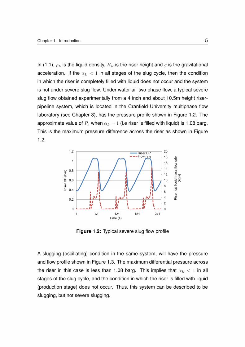
Chapter 1. Introduction 5
In (1.1), ρL is the liquid density, HR is the riser height and g is the gravitational
acceleration. If the αL < 1 in all stages of the slug cycle, then the condition
in which the riser is completely filled with liquid does not occur and the system
is not under severe slug flow. Under water-air two phase flow, a typical severe
slug flow obtained experimentally from a 4 inch and about 10.5m height riser-
pipeline system, which is located in the Cranfield University multiphase flow
laboratory (see Chapter 3), has the pressure profile shown in Figure 1.2. The
approximate value of Ph when αL = 1 (i.e riser is filled with liquid) is 1.08 barg.
This is the maximum pressure difference across the riser as shown in Figure
1.2.
0
2
4
6
8
10
12
14
16
18
20
0
0.2
0.4
0.6
0.8
1
1.2
1 61 121 181 241
Ris
er
DP
(ba
r)
Riser DPFlow rate
Time (s)
Ris
er
top
liqu
idm
ass
flo
wra
te(k
g/s
)
Figure 1.2: Typical severe slug flow profile
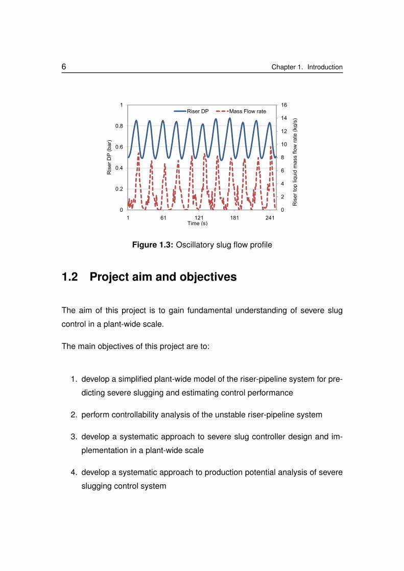
A slugging (oscillating) condition in the same system, will have the pressure
and flow profile shown in Figure 1.3. The maximum differential pressure across
the riser in this case is less than 1.08 barg. This implies that αL < 1 in all
stages of the slug cycle, and the condition in which the riser is filled with liquid
(production stage) does not occur. Thus, this system can be described to be
slugging, but not severe slugging.
6 Chapter 1. Introduction
0
2
4
6
8
10
12
14
16
0
0.2
0.4
0.6
0.8
1
1 61 121 181 241
Ris
er
DP
(ba
r)Riser DP Mass Flow rate
Time (s)
Ris
er
top
liqu
idm
ass
flow
rate
(kg/s
)
Figure 1.3: Oscillatory slug flow profile
1.2 Project aim and objectives
The aim of this project is to gain fundamental understanding of severe slug
control in a plant-wide scale.
The main objectives of this project are to:
1. develop a simplified plant-wide model of the riser-pipeline system for pre-
dicting severe slugging and estimating control performance
2. perform controllability analysis of the unstable riser-pipeline system
3. develop a systematic approach to severe slug controller design and im-
plementation in a plant-wide scale
4. develop a systematic approach to production potential analysis of severe
slugging control system
Chapter 1. Introduction 7
5. carry out laboratory demonstrations of severe slug control using designed
controllers
1.3 Methodology
In this section, the methodologies applied in this research project are explained.
The project adopts model based and experimental analysis methodology. As
a result, the methodology involves four major areas which includes: modeling,
simulation, experimentation and validation.
Modeling
The accurate prediction of severe slugging characteristics and control perfor-
mance are key requirements for this project. As a result, the modeling of the
riser induced severe slugging is performed using mechanistic modeling of the
riser-pipeline system in a plant-wide scale. Using a basic simplified riser model
(SRM) which had been developed by Storkaas [102], an improved simplified
riser model(ISRM) is developed, with improved performance and more reliable
results achieved, when compared to experimental results. The ISRM is pro-
grammed in the Matlab/Simulink software. The 2 inch, 4 inch and the indus-
trial riser-pipeline systems used in the project are all modeled using the ISRM.
These systems are described in Chapter 3. It should be mentioned here that in
order to simulate the real field behaviour of these systems, a linear well model
and a two phase separator model have also been developed and linked with
the ISRM.
8 Chapter 1. Introduction
Simulation
Software simulations are carried out using the commercial multiphase flow sim-
ulator, OLGA, which is developed by the SPT Group [37]. Two riser-pipeline
systems are modeled in the OLGA software. These two riser systems include,
an industrial riser-pipeline system and the 4 inch riser-pipeline system which
is used in the experimental studies. The industrial riser-pipeline system is a
standard system which was provided by the SPT Group. The configuration and
operating conditions of the industrial riser system is described in section 3.5.
Experiment
In this project, experimental studies have been carried out on two riser-pipeline
systems. The two riser-pipeline systems are the 2 inch and the 4 inch riser-
pipeline systems, which are flow loops in the multiphase flow laboratory at
Cranfield University. The configuration and operating conditions of these sys-
tems are described in Chapter 3.
Analyses and validation
Various analyses are performed for understanding of the system and validation.
These analyses include, severe slug characteristics, controllability, controller
design, control performance, control impact and production analysis.

Chapter 1. Introduction 9
1.4 Thesis outline and contributions
The work presented in this thesis is outlined according to the chapters as fol-
lows:
Chapter 2
In this chapter, a review of multiphase slug flow and the current severe slug-
ging control technologies and their applications is presented. Firstly, a general
overview of multiphase flow and slug flow is presented. This is followed by de-
tailed discussions of the underlying principles of operation of severe slugging
control technologies. Their limitations and challenges are also discussed.
Chapter 3
In this chapter, the description of the experimental facility and the industrial riser
system used in this work is presented. The description of the relevant operating
conditions and the pipeline dimensions are also presented.
Chapter 4
In this chapter, the modeling of the major system units of the riser-pipeline sys-
tem to develop the plant-wide model, which is required for severe slug flow
prediction and control performance analysis is presented. The modeling of the
riser-pipeline system and its integration with the model of the two phase sep-
arator system and the pressure dependent well model is achieved. Through
the development of the plant-wide model, an improved simplified riser model
(ISRM) is developed to eliminate some assumptions and limitations of an origi-
nal simplified riser model (SRM) in predicting severe slugging. The ability of the
ISRM to predict nonlinear stability of the system is investigated using the indus-
10 Chapter 1. Introduction
trial riser system and a 4 inch laboratory riser system. The ISRM prediction of
these nonlinear stabilities showed close agreement with experimental results,
than the SRM.
Chapter 5
In this chapter, the controllability analysis of the unstable riser-pipeline system
which is focused on the ability to achieve stable operation and maximise pro-
duction is presented. A more appropriate slug control strategy is implemented
to show that some controlled variables which had been considered unsuitable
for slug control can in practice be used to stabilise the unstable riser-pipeline
system. In this control strategy, the perfect tracking of controlled variable set
point ideology is neglected and the unstable riser system is stabilised at a ref-
erence valve opening using a derivative controller, whose control input is the
controlled variable. The lower bound of the control input magnitude required
to stabilise the system at the open-loop unstable operating points is evaluated
as a function of the Hankel singular value of the system’s linear model trans-
fer function. This controllability analysis reveals the ability of various controlled
variable to stabilise the unstable riser-pipeline system at relatively large valve
opening.
Chapter 6
In this chapter, a new concept known as the production gain index (PGI) anal-
ysis, which is used for the systematic analysis of the potential of the slug con-
trol system to maximise production in an unstable riser-pipeline system is pre-
sented. This systematic method, which is based on the pressure bifurcation
map of a riser system is applied to analyse the production and pressure loss
relationship at the different operating points. This analysis has been success-
fully applied to an industrial riser system, which was modeled in the commer-
Chapter 1. Introduction 11
cial multiphase flow simulator, OLGA. The prediction of production gain or loss
using the PGI agrees with actual simulated production. This result is very sig-
nificant in planning and implementing suitable control strategy for stabilising
unstable riser-pipeline production systems with the aim of achieving stability
and ensuring increased productivity, especially for brown fields.
Chapter 7
In this chapter, the design, characterisation, implementation and the perfor-
mance analysis of three active slug controllers for maximising oil production
is presented. The three active slug controllers namely: the relay auto-tuned
controller, the robust PID controller and the H∞ robust controller are designed,
characterised and implemented under the same operating condition for two
controlled variables; PRB and QT . A principle for characterising the ability of
a slug controller to achieve closed-loop stability at large valve opening in the
open-loop unstable operating point, using the ‖T‖∞ is presented. It is shown
that the H∞ robust slug controller which achieved the lowest value of the ‖T‖∞,
achieved closed-loop stability at a larger valve opening than the relay auto-
tuned slug controller, which achieved the highest value of the ‖T‖∞.
Chapter 8
In this chapter, the development of an improved relay auto-tuned slug controller
algorithm is achieved to improve the poor performance of the relay auto-tuned
slug controller in Chapter 6. The developed controller algorithm is based on
a perturbed FOPDT model of the riser system, obtained through relay shape
factor analysis. The developed controller algorithm is implemented on the in-
dustrial riser system to show that it has the ability to stabilise the unstable riser
system at a valve opening that is larger than that achieved with the original
(conventional) design algorithm with about 4% increase in production.
12 Chapter 1. Introduction
Chapter 9
The conclusion and summary of the work and results presented in the thesis
are presented in this chapter.
1.5 Publications
The following publications have resulted from this work.
1.5.1 Conference papers
Chapter 3 and 6
Ogazi, A. I., Ogunkolade, S., Cao, Y., Lao, L., and Yeung, H. Severe slug-
ging control through open-loop unstable PID tuning to increase oil production.
In 14th International Conference on Multiphase Technology (Cannes, France,
June 2009), BHR Group, pp. 17-32.
Chapter 6
Ogazi, A.I., Cao, Y., Yeung, H., and Lao, L. . Slug control with large valve
opening to maximise oil production. In SPE Offshore Europe Conference, SPE
124883,(2009)
Ogazi, A.I., Cao, Y., Yeung, H., and Lao, L. Robust Control of severe slugging to
maximise oil production. In International Conference on System Engineering,
2009 Conference, (Conventry, UK, 2009).
Chapter 1. Introduction 13
Chapter 5
Ogazi, A.I., Cao, Y., Yeung, H., and Lao, L. Production potential of a severe
slugging control system. IFAC World Congress (Milan Italy, September, 2011)
(to be presented).
1.5.2 Journal paper
Chapter 6
Ogazi, A.I., Cao, Y., Yeung, H., and Lao, L. . Slug control with large valve
opening to maximise oil production. SPE Journal, SPE 124883,(2010), 15(3),
812-821.

14 Chapter 1. Introduction
Chapter 2
Literature review
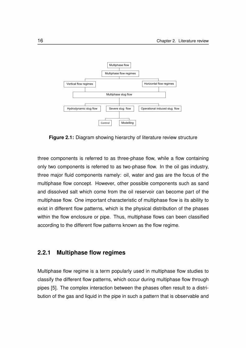
2.1 Introduction
In this Chapter, the review of the relevant literatures on severe slugging control
is presented. Firstly, a general overview of multiphase flow is presented with
the relevant literatures. This is followed by a review of the flow regime maps,
and then slug flow. A review of the current severe slugging control technolo-
gies and their applications is then presented. This begins with classification of
pipeline slugging and detailed description of the slug control techniques and
the underlying technology is then provided. The hierarchal structure for the
literature review is laid out in Figure 2.1 for clarity.
2.2 Multiphase flow
As the name implies, a flow is said to be a multiphase flow when it contains
more than one fluid phase, which are flowing simultaneously in the same con-
duit or an enclosure, such as a pipe [16, 13]. A multiphase flow containing any
15
16 Chapter 2. Literature review
Multiphase flow
Vertical flow regimes Horizontal flow regimes
Modelling
Multiphase slug flow
Control
Operational induced slug flowHydrodynamic slug flow Severe slug flow
Multiphase flow regimes
Figure 2.1: Diagram showing hierarchy of literature review structure
three components is referred to as three-phase flow, while a flow containing
only two components is referred to as two-phase flow. In the oil gas industry,
three major fluid components namely: oil, water and gas are the focus of the
multiphase flow concept. However, other possible components such as sand
and dissolved salt which come from the oil reservoir can become part of the
multiphase flow. One important characteristic of multiphase flow is its ability to
exist in different flow patterns, which is the physical distribution of the phases
within the flow enclosure or pipe. Thus, multiphase flows can been classified
according to the different flow patterns known as the flow regime.
2.2.1 Multiphase flow regimes
Multiphase flow regime is a term popularly used in multiphase flow studies to
classify the different flow patterns, which occur during multiphase flow through
pipes [5]. The complex interaction between the phases often result to a distri-
bution of the gas and liquid in the pipe in such a pattern that is observable and
Chapter 2. Literature review 17
can be represented using a flow map known as flow regime map. In generating
the flow regime map, a good number of investigation is carried out to determine
the dependency of flow patterns on the volume fraction of the components of
the multiphase flow [17]. Although multiphase flow regimes can be studied for
two-phase gas-liquid flows and for three-phase oil-water-gas flows, this review
will focus mainly on the two-phase gas-liquid flow.
One of the limitation of flow regime maps is that they are only relevant to the
system (pipeline dimension, operating condition and fluid type) applied in gen-
erating it [13]. This implies that no one flow regime can be applied to interpret
flow pattern in all flow systems. Previous works such as that by Schicht [87],
Weisman and Kang [115], which was aimed at generalising flow regime map
coordinates has not been successful because the transition in most flow regime
maps and the corresponding instabilities depend on different properties of the
fluid.
The flow pattern predominant in a vertical pipeline vary from that of the hori-
zontal pipeline [115]. For example, while a stratified flow pattern observed in
the horizontal pipe flow is not observed in the vertical pipe flow, the churn flow
observed in the vertical pipe flow is not observed in the horizontal pipe flow.
Thus, the flow regime in the vertical and horizontal pipe are discussed.
2.2.1.1 Multiphase two-phase gas-liquid flow regimes in horizontal pipe
The flow patterns generated during multiphase flow through horizontal pipes
has been studies in reasonable details over the years. One of the earliest
study on flow regime in horizontal pipes was reported by Baker [5] and Hoogen-
doorn [45]. Recently, a number of other studies on two-phase gas-liquid hor-
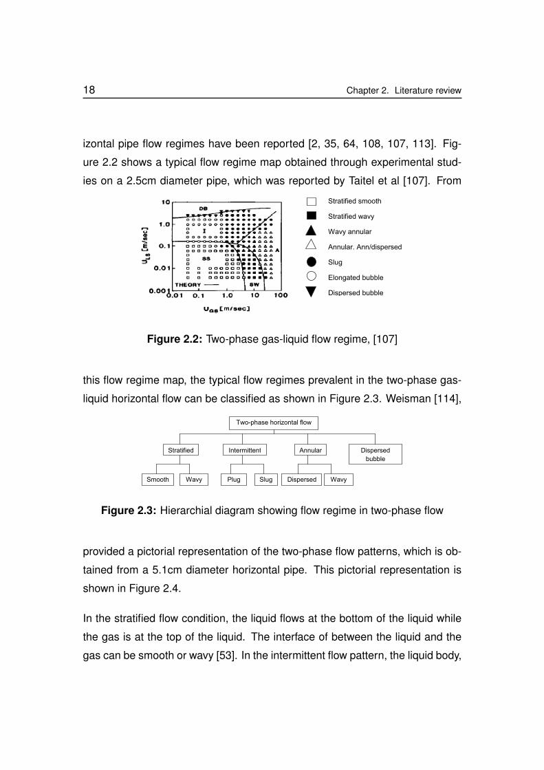
18 Chapter 2. Literature review
izontal pipe flow regimes have been reported [2, 35, 64, 108, 107, 113]. Fig-
ure 2.2 shows a typical flow regime map obtained through experimental stud-
ies on a 2.5cm diameter pipe, which was reported by Taitel et al [107]. From
Stratified smooth
Stratified wavy
Wavy annular
Annular. Ann/dispersed
Slug
Elongated bubble
Dispersed bubble
Figure 2.2: Two-phase gas-liquid flow regime, [107]
this flow regime map, the typical flow regimes prevalent in the two-phase gas-
liquid horizontal flow can be classified as shown in Figure 2.3. Weisman [114],
Two-phase horizontal flow
Stratified Intermittent Annular Dispersed
bubble
Smooth Wavy Plug Slug Dispersed Wavy
Figure 2.3: Hierarchial diagram showing flow regime in two-phase flow
provided a pictorial representation of the two-phase flow patterns, which is ob-
tained from a 5.1cm diameter horizontal pipe. This pictorial representation is
shown in Figure 2.4.
In the stratified flow condition, the liquid flows at the bottom of the liquid while
the gas is at the top of the liquid. The interface of between the liquid and the
gas can be smooth or wavy [53]. In the intermittent flow pattern, the liquid body,
Chapter 2. Literature review 19
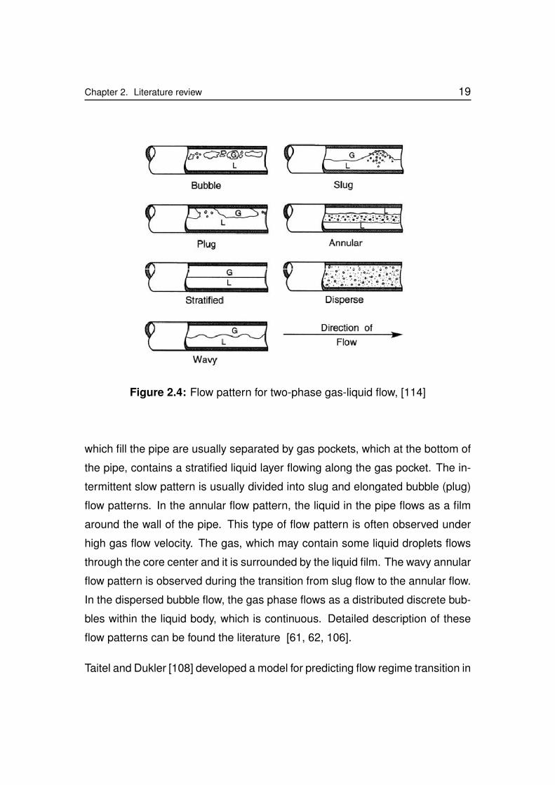
Figure 2.4: Flow pattern for two-phase gas-liquid flow, [114]
which fill the pipe are usually separated by gas pockets, which at the bottom of
the pipe, contains a stratified liquid layer flowing along the gas pocket. The in-
termittent slow pattern is usually divided into slug and elongated bubble (plug)
flow patterns. In the annular flow pattern, the liquid in the pipe flows as a film
around the wall of the pipe. This type of flow pattern is often observed under
high gas flow velocity. The gas, which may contain some liquid droplets flows
through the core center and it is surrounded by the liquid film. The wavy annular
flow pattern is observed during the transition from slug flow to the annular flow.
In the dispersed bubble flow, the gas phase flows as a distributed discrete bub-
bles within the liquid body, which is continuous. Detailed description of these
flow patterns can be found the literature [61, 62, 106].
Taitel and Dukler [108] developed a model for predicting flow regime transition in
20 Chapter 2. Literature review
horizontal and nearly horizontal pipe with two-phase gas-liquid flow. In a later
work by Taitel et al [107], the model result was compared with experimental
results and good agreement between the two was concluded. A model for
predicting pressure distribution for two-phase flow through inclined, vertical and
curved pipes was also developed by Gould et al [34].
Further studies has also been carried out on the effect of pipeline inclination
on flow regime of two-phase flow in horizontal pipes [8, 11, 34, 36, 93, 107].
The work by Taitel et al [107] reported the effect of pipe inclination on the flow
regime map. They showed that small deviation (inclination) from the horizontal
have significant effect on the flow regime map. The effect of pipe inclination
on the liquid holdup and the pressure loss across the pipe was investigated
by Beggs and Brill [8]. Gould et al [34] also reported flow pattern maps for
horizontal and vertical flows with pipe inclination for upflow at 45o.
2.2.1.2 Multiphase two-phase flow regimes in vertical pipe
The flow regimes identified in vertical pipelines are often different from that
of the horizontal pipeline [115]. The challenge of the lack of a universal flow
regime map for interpreting two-phase flow in the vertical pipes still exist. This
is due to the significant effect of phase properties and the pipe diameters on
multiphase flow regimes [96]. Despite these limitations, the main types of flow
regimes, which are identified in the vertical pipeline include the bubbly flow, the
slug flow, the churn flow and the annular flow [66]. Figure 2.5 shows typical
flow patterns and the flow regime map obtained from a 72mm diameter vertical
pipe, reported by Guet and Ooms [38].
The modeling and experimental work to predict and describe these flow regimes

Chapter 2. Literature review 21
Figure 2.5: Flow pattern for two-phase gas-liquid vertical flow, [38]
can be found in many literatures [66, 68, 73, 96, 105, 115]. The bubble flow rep-
resents a flow pattern in which the gas phase flows as a small discrete bubbles
in a continuous liquid phase [115]. The slug flow pattern occur due to the co-
alescence of the gas bubbles at increased gas flowrate, which results to bullet
type gas pocket, known as Taylor bubbles [96]. The Taylor bubble is usually
separated by liquid slug, which often contain some gas bubbles in the liquid
body. The diameter of the Taylor bubble often correspond to the diameter of the
pipe, but the Taylor bubble is usually surrounded by a thin of liquid film, which
flows vertically downwards. The churn flow is formed due to the break up of
Taylor bubble into the liquid body as the gas flowrate increases [52]. The churn
flow is predominantly a disorderly flow regime, in which the liquid is observed
to flow vertically upwards in an oscillatory motion. The annular flow regime oc-
curs when the gas flowrate is further increased such that the gas flows in the
core of the pipe and the liquid flows around the pipe walls [66]. The gas flowing
through the pipe core can also carry liquid droplets, which are dispersed in it.
22 Chapter 2. Literature review
2.3 Multiphase slug Flow
Slug flow is one of the most undesired multiphase flow regimes, due to the
associated instability which imposes a major challenge to flow assurance in the
oil and gas industry. The oil and gas industry encounters slug flow in the course
of their production activities. As was discussed in sections 2.2.1.1 and 2.2.1.2,
slug flow occur both in horizontal and vertical pipes. Thus, there are different
types of slugs, which can be distinguished from each other by mechanism of
formation. Thus, the multiphase slug flow can be classified into three different
types, based on the formation mechanism [91, 32]. The three types include:
1. hydrodynamic slugging
2. operation induced slugging
3. severe slugging
2.3.1 Hydrodynamic slugging
Hydrodynamic slug flow, which occur mainly in horizontal pipes is initiated from
stratified flow due to two broad hydrodynamic mechanisms, namely: the natural
growth of hydrodynamic wave instabilities generated on the gas-liquid interface,
and the accumulation of liquid caused by sudden pressure and gravitational
force imbalance, due to undulation in the pipeline geometry [47]. The growth
of hydrodynamic wave instabilities has been described to depend on the clas-
sical KelvinHelmholtz (KH) instability mechanism [27, 28, 56, 60]. Arnaud et al
investigated the effects of wave interaction on the formation of hydrodynamic
slugs in two-phase pipe flow at relatively low gas and liquid superficial veloci-
Chapter 2. Literature review 23
ties. They conducted their experiments in a horizontal pipe, which is 31m long,
10cm internal diameter at atmospheric pressure. They found that the formation
of hydrodynamic slugs due to wave interaction differs from predictions for slug
formation using long wavelength stability theory.
The study of hydrodynamic slug flow has resulted to the development of a num-
ber of transient and steady state models. Isaa and Kempf [47] suggested the
classification of the transient models into three categories namely: empirical
slug specification, slug tracking, and slug capturing models. While the empirical
slug specification models are used to describe various stages of slug develop-
ment including slug formation, growth, decay and slug shape [108, 25], the slug
tracking models are used to track the movement, the growth and the dissipation
of individual slugs in the slug flow [9]. A slug tracking technique, which is ca-
pable of predicting slug generation, slug growth, and slug dissipation was also
developed by Zheng et al [117]. The capturing models are developed to predict
slug flow regimes using mechanistic and automatic results of the hydrodynamic
growth instabilities [48].
2.3.2 Operation induced slug
This type of slug is induced due to certain operations performed during pro-
duction. Operations such as ramp-up (increasing production), pigging and de-
pressurisation can generate a huge number of liquid slugs.
24 Chapter 2. Literature review
2.3.3 Severe slugging
This type of slug flow is caused by the undulations and dips in the pipeline
geometry, topography and network [82]. Towards the end of the operational life
of an oil reservoir, the reservoir pressure can become depleted or the Gas-to-
liquid ratio (GLR) can become very low. In such conditions, the gravitational
pressure dominates the flow resistance, and liquid accumulates at the pipe
dips, thereby blocking the flow channel and preventing gas flow. This process
results to intermittent flow condition. This intermittent flow condition, which is
characterised by pockets of liquid and gas flow followed by no liquid and gas
flow out of the riser is referred to as severe slugging [70, 72]. The severe slug
cycle process, which was discussed in section 1.1.2 has been described in
many literatures [7, 18, 43, 59, 70].
The slug lenght produced in a typical severe slug flow is usually equal to or
greater than one riser height [72, 89]. One major challenge associated with
severe slugging is that it is characterized by large pressure and flowrate fluctu-
ations [86]. The associated fluctuations in pressure and flowrate can damage
downstream processing equipment, increase pipeline stress, reduce productiv-
ity and shorten the reservoir operation life [44].
2.3.3.1 Severe slug models
A number of steady state models [33, 82, 108, 103] and transient models
[26, 69, 85, 89, 104] have been developed to predict the occurrence of severe
slugging in a riser-pipeline system. The severe slug models are often devel-
oped to answer some basic questions associated with severe slug flow, such
as:
Chapter 2. Literature review 25
1. at what condition does severe slugging occur and
2. what will be the characteristics of the severe slugging when it occurs?
One of the models reported to predict at what condition severe slugging will
occur was developed to show that a stratified flow regime in the pipeline is a
condition for severe slugging to occur [89]. Taitel and Dukler [108] first devel-
oped a criterion to predict stratified flow regime in horizontal and near horizon-
tal pipelines. By applying the inviscid Kelvin- Helmholtz theory in which shear
stress is neglected [56], the condition given in (2.1) was developed. In (2.1), UGis the superficial gas velocity, hG is height occupied by the gas phase, ρ is den-
sity and the subscripts G and L refer to the gas and liquid phases respectively.
UG >
[g(ρL − ρG)hG
ρG
] 12
(2.1)
When the superficial gas velocity, UG, is lower than that obtained by evaluating
the right-hand-side (RHS) of (2.1), then a stratified flow regime is obtained in
the pipeline and severe slugging can occur in the riser-pipeline system. A plot
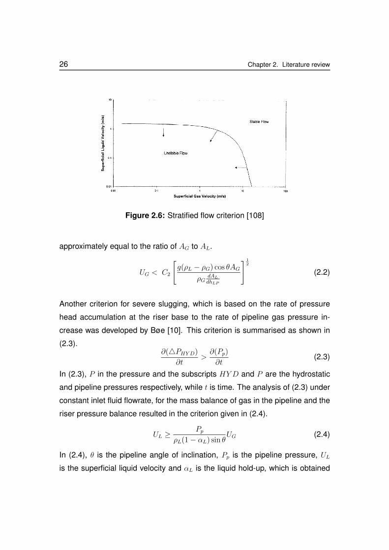
of this criterion as presented by Taitel and Dukler [108], is shown in Figure 2.6.
Below the transition line in Figure 2.6 is the region were stratified flow occur in
the pipeline.
Base on the Taitel and Dukler criterion, Goldzberg and McKee [33] also de-
veloped a criterion for the formation of slug in a pipe dip, by the sweeping out
of the accumulated liquid in the pipe dip. The resulting criterion obtained by
Goldzberg and McKee, which was achieved by analysing the Bernoulli equa-
tion over the liquid surface is given in (2.8), where θ is the angle of inclination
of the pipeline, AL is the liquid flow area, AG is the gas flow area and C2 is
26 Chapter 2. Literature review
Figure 2.6: Stratified flow criterion [108]
approximately equal to the ratio of AG to AL.
UG < C2
[g(ρL − ρG) cos θAG
ρGdALdhLP
] 12
(2.2)
Another criterion for severe slugging, which is based on the rate of pressure
head accumulation at the riser base to the rate of pipeline gas pressure in-
crease was developed by Bøe [10]. This criterion is summarised as shown in
(2.3).∂(4PHYD)
∂t>∂(Pp)
∂t(2.3)
In (2.3), P in the pressure and the subscripts HYD and P are the hydrostatic
and pipeline pressures respectively, while t is time. The analysis of (2.3) under
constant inlet fluid flowrate, for the mass balance of gas in the pipeline and the
riser pressure balance resulted in the criterion given in (2.4).
UL ≥Pp
ρL(1− αL) sin θUG (2.4)
In (2.4), θ is the pipeline angle of inclination, Pp is the pipeline pressure, ULis the superficial liquid velocity and αL is the liquid hold-up, which is obtained
Chapter 2. Literature review 27
assuming no slip condition as given in (2.5). For severe slugging to occur, the
condition in (2.4) must be satisfied.
αL =UL
UL + UG(2.5)
Pots et al [82] also developed another criterion for predicting the occurrence
of severe slugging. Similar to the Bøe’s [10] criterion, the criterion developed
by Pots et al [82] considered the balance between the rate of hydrostatic pres-
sure head build up across the riser and the rate of gas pressure build up in
the pipeline. In the development of the Pots et al criterion given in (2.6), it is
considered that for severe slugging to occur, the rate of hydrostatic pressure
head build up across the riser must be greater than the rate of accumulation of
gas pressure in the pipeline. The analysis of this criterion shows that severe
slugging will occur if Πss < 1. The criterion was developed assuming that there
is no mass transfer between the liquid and gas phase, the riser is vertical and
there is no liquid fall back.
Πss =ZRT/MGmG
gαLLmL
(2.6)
In (2.6), Z is the gas compressibility, MG is the gas molecular weight, mL and
mG is the mass flowrate of liquid and gas respectively.
Another criterion for severe slugging to occur was developed by Taitel [103].
The Taitel’s criterion considered the blow-out stage of the severe cycle process
and the net force across the riser during the blow-out stage. In the Taitel’s
criterion, the condition for severe slugging to occur is given by (2.7). Thus,
severe slugging will occur is 4F increases y, where 4F is the net force over
the riser column, when the gas tail penetrates into the riser at the base, y is the
height of the gas bubble penetrating into the riser.
∂(4F )
∂y> 0 (2.7)

28 Chapter 2. Literature review
The 4F is given by (2.8),
4F =
[(Ps + ρLgHR)
αGL
αGL+ yα′G
]− [Ps + ρLg(HR − y)] (2.8)
where Ps is the topside separator pressure, HR is the riser height, αG is the gas
hold-up in the pipeline, L is the length of the pipeline and α′G is the gas hold-
up in the gas bubble penetrating the riser. By combining (2.7) and (2.8), (2.9),
which is the final form of the criterion, considering the atmospheric pressure is
obtained. Thus, severe slugging will occur if the condition in (2.9) is satisfied.
PsP0
<
(αGα′G
)L−HR
P0/ρLg(2.9)
The analysis of this criterion shows that it depends on the riser-pipeline oper-
ating condition and geometry. The gas hold-up, α′G, is assumed to be equal
to a constant value of 0.89. Fuchs [30] also developed a severe slug criterion
model, which was based on the slug blow out stage analysis.
Schmidt et al [89] with focus on the liquid build up stage developed a transient
model based on mass and pressure balances on the riser-pipeline system.
The purpose of their model was to predict the time for slug build up and the
slug length. Although the model prediction showed good agreement with their
experimental result, the model’s ability to be generalised was very limited due
to the closure model, which was developed as empirical correlations generated
from their experimental facility.
Another transient model for predicting severe slugging was developed by Schmidt
et al [90]. This model was developed with focus on predicting all the stages in
the severe slugging cycle (see section 1.1.2). Similar to the model of Schmidt
et al [89], the model was developed using the mass and pressure balances on
the riser-pipeline system for each stage in the cycle. The gas-liquid interface
were used to define the transition between the stages in the slug cycle. The
Chapter 2. Literature review 29
simulation results obtained from this model was reported to agree closely from
their experimental result. This model developed by Schmidt et al [90] has been
used in subsequent work by Hill [43]. A comprehensive review of transient slug
model was reported by Ozawa and Sakaguchi [79]. They explained that while
slug transport was dominated by gravity in the vertical pipe, in the horizontal
pipe, it was dominated by momentum flux of the liquid at the back of the slug.
2.4 Severe slugging control techniques and tech-
nologies
Severe slugging has become a major challenge to gathering crude oil from the
fast depleting oil reservoirs. With deepwater exploration up to 2000m becom-
ing common, many risers will be required in the coming decade, all of which
will become vulnerable to severe slugging if a sustainable solution is not found.
A number of severe slugging control techniques have been proposed based
on experimental, theoretical and field studies. This section reviews these se-
vere slugging control techniques and their objectives based on the underlying
technologies. The current control techniques can be classified into two, based
on the underlying scientific and/or technological principles employed. The two
classifications are:
1. changing flow condition
2. riser outlet downstream adjustment
30 Chapter 2. Literature review
2.4.1 Changing flow condition
This approach focuses on altering the flow, pressure conditions and the struc-
ture of the flowline upstream (sub-sea) of the riser. Current practical approaches
include:
1. design modification of upstream facilities
2. riser base gas lift
3. gas re-injection (self-lifting)
4. homogenising the multiphase flow
5. subsea separation and processing
2.4.1.1 Design modification of upstream facilities
This method involves applying changes to the existing facilities upstream of
the riser. The common concepts are: changing flowline internal diameter and
changing pipeline layout structure.
Changing flowline internal diameter
In order to mitigate the severe slugging occurring in a production system, the
pipeline size can be changed with targets on increasing or reducing the internal
pipe diameter, depending on the type of slug prevalent in the system. Reduc-
ing the pipe diameter, will reduce the cross sectional area of the pipe thereby
increasing the fluid velocity. This concept generates a flow regime with low
gravitational pressure drop in the riser, a condition necessary for avoiding liquid
Chapter 2. Literature review 31
accumulation at the riser base which is prevalent in low velocity terrain induced
severe slugging. Increasing the pipe diameter increases the cross sectional
area of the pipe. This may produce a low velocity stratified flow in the flowline,
a condition necessary for avoiding hydrodynamic slug. This implies that while
increasing pipe diameter may remove hydrodynamic slug, it may initiate terrain
induced slug and vice versa.
Fargharly [29] concluded in a study of severe slugging in the Upper Zakum oil
field that optimum sizing may alleviate (mitigate) the severe slugging problem
but it will not eliminate severe slugging completely. However, optimal sizing
will depend on other production factors which could be difficult to determine
precisely. One disadvantage of this method is that changing flowline diameter is
capital intensive and it may introduce other operational problems. This reduces
the chances of implementing this strategy.
Changing pipeline geometry
Makogan and Brook [63] of BP patented a slug mitigation device which they
claim can inhibit severe slugs. The device is a specially designed pipe which
has an upward inclined part, a horizontal part and a downward inclined part.
The device is positioned immediately upstream of the riser as shown in Figure
2.7. They claim that the device inhibits severe slugging by reducing the length
of the liquid slugs as well as increasing the frequency of the discrete liquid
slugs. This enables the gas pressure behind the slug to be sufficient enough
to drive the slug through the riser. As a result, plug (intermittent) flow regime is
generated. It is claimed that the produced intermittent flow can be handled by
the topside facilities.
There is no field or experimental results reported on the effectiveness of this de-
vice. The device, on examination can be considered as a mini-riser which may
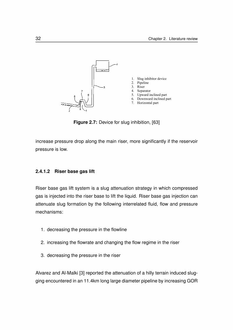
32 Chapter 2. Literature review
1. Slug inhibitor device2. Pipeline3. Riser4. Separator5. Upward inclined part6. Downward inclined part7. Horizontal part
Figure 2.7: Device for slug inhibition, [63]
increase pressure drop along the main riser, more significantly if the reservoir
pressure is low.
2.4.1.2 Riser base gas lift
Riser base gas lift system is a slug attenuation strategy in which compressed
gas is injected into the riser base to lift the liquid. Riser base gas injection can
attenuate slug formation by the following interrelated fluid, flow and pressure
mechanisms:
1. decreasing the pressure in the flowline
2. increasing the flowrate and changing the flow regime in the riser
3. decreasing the pressure in the riser
Alvarez and Al-Malki [3] reported the attenuation of a hilly terrain induced slug-
ging encountered in an 11.4km long large diameter pipeline by increasing GOR
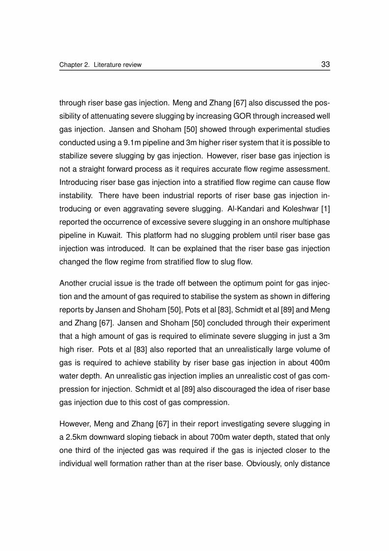
Chapter 2. Literature review 33
through riser base gas injection. Meng and Zhang [67] also discussed the pos-
sibility of attenuating severe slugging by increasing GOR through increased well
gas injection. Jansen and Shoham [50] showed through experimental studies
conducted using a 9.1m pipeline and 3m higher riser system that it is possible to
stabilize severe slugging by gas injection. However, riser base gas injection is
not a straight forward process as it requires accurate flow regime assessment.
Introducing riser base gas injection into a stratified flow regime can cause flow
instability. There have been industrial reports of riser base gas injection in-
troducing or even aggravating severe slugging. Al-Kandari and Koleshwar [1]
reported the occurrence of excessive severe slugging in an onshore multiphase
pipeline in Kuwait. This platform had no slugging problem until riser base gas
injection was introduced. It can be explained that the riser base gas injection
changed the flow regime from stratified flow to slug flow.
Another crucial issue is the trade off between the optimum point for gas injec-
tion and the amount of gas required to stabilise the system as shown in differing
reports by Jansen and Shoham [50], Pots et al [83], Schmidt et al [89] and Meng
and Zhang [67]. Jansen and Shoham [50] concluded through their experiment
that a high amount of gas is required to eliminate severe slugging in just a 3m
high riser. Pots et al [83] also reported that an unrealistically large volume of
gas is required to achieve stability by riser base gas injection in about 400m
water depth. An unrealistic gas injection implies an unrealistic cost of gas com-
pression for injection. Schmidt et al [89] also discouraged the idea of riser base
gas injection due to this cost of gas compression.
However, Meng and Zhang [67] in their report investigating severe slugging in
a 2.5km downward sloping tieback in about 700m water depth, stated that only
one third of the injected gas was required if the gas is injected closer to the
individual well formation rather than at the riser base. Obviously, only distance
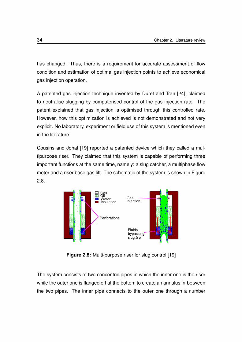
34 Chapter 2. Literature review
has changed. Thus, there is a requirement for accurate assessment of flow
condition and estimation of optimal gas injection points to achieve economical
gas injection operation.
A patented gas injection technique invented by Duret and Tran [24], claimed
to neutralise slugging by computerised control of the gas injection rate. The
patent explained that gas injection is optimised through this controlled rate.
However, how this optimization is achieved is not demonstrated and not very
explicit. No laboratory, experiment or field use of this system is mentioned even
in the literature.
Cousins and Johal [19] reported a patented device which they called a mul-
tipurpose riser. They claimed that this system is capable of performing three
important functions at the same time, namely: a slug catcher, a multiphase flow
meter and a riser base gas lift. The schematic of the system is shown in Figure
2.8.
Fluidsbypassingslug Δ p
GasInjection
Perforations
GasOilWaterInsulation
Figure 2.8: Multi-purpose riser for slug control [19]
The system consists of two concentric pipes in which the inner one is the riser
while the outer one is flanged off at the bottom to create an annulus in-between
the two pipes. The inner pipe connects to the outer one through a number
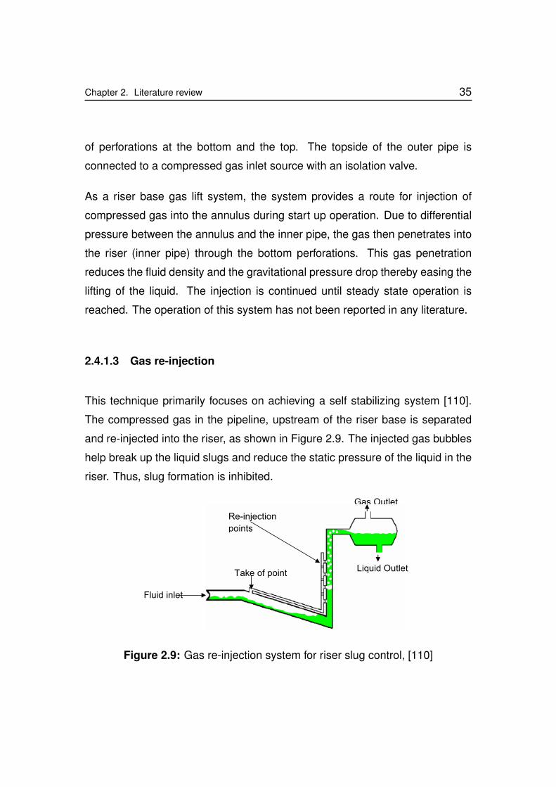
Chapter 2. Literature review 35
of perforations at the bottom and the top. The topside of the outer pipe is
connected to a compressed gas inlet source with an isolation valve.
As a riser base gas lift system, the system provides a route for injection of
compressed gas into the annulus during start up operation. Due to differential
pressure between the annulus and the inner pipe, the gas then penetrates into
the riser (inner pipe) through the bottom perforations. This gas penetration
reduces the fluid density and the gravitational pressure drop thereby easing the
lifting of the liquid. The injection is continued until steady state operation is
reached. The operation of this system has not been reported in any literature.
2.4.1.3 Gas re-injection
This technique primarily focuses on achieving a self stabilizing system [110].
The compressed gas in the pipeline, upstream of the riser base is separated
and re-injected into the riser, as shown in Figure 2.9. The injected gas bubbles
help break up the liquid slugs and reduce the static pressure of the liquid in the
riser. Thus, slug formation is inhibited.
Fluid inlet
Liquid Outlet
Gas Outlet
Take of point
Re-injection
points
Figure 2.9: Gas re-injection system for riser slug control, [110]
36 Chapter 2. Literature review
Further studies have considered different locations for gas re-injection and a
basic regulatory control is included to manipulate the gas re-injection for op-
timisation [110]. Tengesdal et al [110] reported various experimental results
focused on identifying the optimal injection point. He concluded that the ideal
injection point is at the same level or slightly higher than the take off point.
The pressure drop in the by-pass system must be higher than the static head
above the injection point, less liquid would block the injection pipe. To achieve
this, a ball valve is installed at the injection line for backpressure build up when
throttled. Another location considered is the gas bypass as shown in Figure
2.10.
Separator
Liquid out
Gas out
Valve
By pass
Pipeline
Gas
Liquid
Riser
Figure 2.10: Gas by-pass method
The major advantage of this process is that it can prevent slug formation without
an additional gas supply. However, the provision of additional control for the ball
valves could be a limitation. Modification to an existing platform (well) can be
expensive as it may involve major structural changes.
Chapter 2. Literature review 37
2.4.1.4 Homogenising the multiphase flow
Another method of attenuating slug formation is homogenising the mixture. The
objective would be to force the gas and liquid into a homogeneous fluid. This
will eliminate the intermittent flow regime associated with non-homogeneous
multiphase flow. Hassanein and Fairhurst [39] suggested that this can be
achieved by reducing the surface tension of the fluid by injecting a surface ten-
sion reducing surfactant into the flowline. This will change the fluid into foam,
making the fluid homogeneous. The limitation with this method is that it would
increase separation difficulty at the topside and reduce product quality. An-
other method would be the use of intrusive inline mixer in the flow line. This
method would avoid the separation problems but may increase pressure drop
and cause pigging problems.
2.4.1.5 Sub-sea separation of multiphase fluid
This method employs sub-sea separation facilities to separate the fluid into
single phase, liquid and gas. Thus, two separate pipelines for gas and liquid
are required. A subsea pump is also required to provide the pressure head
needed to deliver the liquid to the topside. Consequently, this method avoids
multiphase flow and severe slugging is prevented.
38 Chapter 2. Literature review
2.4.2 Riser outlet downstream adjustment
This approach focuses on altering the flowrate, flow regime, pressure and struc-
ture of the downstream (topside) system. Practical approaches include:
1. design modification of processing facilities
2. topside choke manipulation
i fixed choking
ii dynamic choking
2.4.2.1 Design modification of processing facilities
Modifying the system with the installation of slug catcher(s) is one way to miti-
gate the effect of severe slugging. Slug catchers are enclosed vessels specially
designed and installed at the end of a riser or a pipeline to receive and buffer
liquid slugs. They also provide the first stage of separation and are often re-
ferred to as pre-separators. A schematic diagram of a horizontal slug catcher
is shown in Figure 2.11. They are designed with the capacity to receive and
dampen slug surges thereby protecting the downstream systems. As a slug
mitigation system, slug catchers do not inhibit slug formation.
The addition of control systems to the slug catcher can improve or reduce its
performance. A slug catcher with controlled liquid level would pass the high
liquid surge to the processing facility in order to maintain set liquid level. This
makes the slug catcher ineffective. On the other hand, a slug catcher with
a controlled liquid drain rate will protect the downstream equipment, but such
a slug catcher must have a volume large enough to contain the accumulated
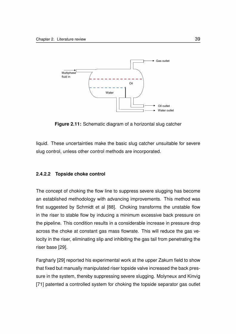
Chapter 2. Literature review 39
Gas
Water
Oil
Water
Water outlet
Oil outlet
Gas outlet
Multiphase
fluid in
Figure 2.11: Schematic diagram of a horizontal slug catcher
liquid. These uncertainties make the basic slug catcher unsuitable for severe
slug control, unless other control methods are incorporated.
2.4.2.2 Topside choke control
The concept of choking the flow line to suppress severe slugging has become
an established methodology with advancing improvements. This method was
first suggested by Schmidt et al [88]. Choking transforms the unstable flow
in the riser to stable flow by inducing a minimum excessive back pressure on
the pipeline. This condition results in a considerable increase in pressure drop
across the choke at constant gas mass flowrate. This will reduce the gas ve-
locity in the riser, eliminating slip and inhibiting the gas tail from penetrating the
riser base [29].
Fargharly [29] reported his experimental work at the upper Zakum field to show
that fixed but manually manipulated riser topside valve increased the back pres-
sure in the system, thereby suppressing severe slugging. Molyneux and Kinvig
[71] patented a controlled system for choking the topside separator gas outlet
40 Chapter 2. Literature review
valve to stabilise severe slugging in a vertical riser. Choking can be broadly di-
vided into two categories namely: fixed choking and dynamic (controlled) chok-
ing.
Fixed choke
Taitel [103] used stability criteria to define a theoretical severe slugging control
law which relates the back pressure to the slug tail propagation into the riser.
With a good approximation, the position of the valve required to stabilize the
system can be pre-calculated and little movement of the valve is required to
maintain quasi-equilibrium in the system. Due to the non-linear nature of mul-
tiphase flow, the application of fixed choke to eliminate severe slugging may
have severe consequences during sudden operational changes. Sudden op-
erational changes can cause the system to become either stable or unstable,
depending on the nature of the changes occurring in the system. While an
unstable system condition is obviously unacceptable and would require imme-
diate control action, a stable system condition may also require control action.
This is because the operating condition of such stable system may occur at a
valve opening that is lower than necessarily required to achieve the same sta-
ble condition. Thus, in order to stabilise the system at the best possible valve
opening, transient flow instabilities require dynamic choke adjustment. Without
this, unnecessary high flowline pressure can occur in the system. This could
lead to losses in production and increased pipeline stress. Dynamic choking
is therefore preferred as an efficient option to controlling slugging problems in
riser-pipeline systems.
Chapter 2. Literature review 41
Dynamic choke
Dynamic choke is a choke manipulated by active control based on real time
changes of system variables. The choking position is not fixed but adjusted
based on a measured variable for achieving stability. Riser base pressure, riser
top pressure and flow rate are commonly adopted control variables. Current
applications of these controlled variables are discussed below.
Riser base pressure control
Many reports on using the riser base pressure as a control variable have shown
its suitability in slug control. Storkaas and Skogestad [101], Drengstig and
Magndal [23], Molyneux and Kinvig [71] and Henriot et al [42] all described
severe slugging suppression using the riser base pressure measurement.
Storkaas and Skogestad [99] applied a systematic analysis of the riser-pipeline
system using control theories. The analysis also included the assessment of
the stability characteristics of the system using the riser top valve opening as
the manipulated variable. Based on their analysis, they identified the riser base
pressure as the best variable for stabilizing riser-pipeline system. This is be-
cause the corresponding transfer function has no right half plane zero which
limits control performance.
Drengstig and Magndal [23] implemented a simple PI controller by measur-
ing both the riser base and the riser top pressure and the using the pressure
difference as the controlled variable while the riser top valve opening as the
manipulated variable. Their report also pointed out that the riser base pressure
is the optimum variable for the slug control.
Molyneux and Kinvig [71] reported a difference in the performance observed in
42 Chapter 2. Literature review
the application of their patented slug control system in a transient multiphase
flow simulation software to that obtained from a test rig. While the controller
achieved only 50% reduction in test rig pressure fluctuation, the simulation sta-
bilised the system. They attributed this difference to the incompleteness of the
transient model used.
Henriot et al [42] reported the simulation studies performed on the Dunbar-
Alwyn pipeline using TACITE multiphase simulator. Having considered various
options to control flow instabilities in the riser, the riser base pressure was con-
sidered most appropriate and used as the controlled variable while the riser
topside valve opening was used as the manipulated variable. When there is a
pressure build up at the riser base, the control system reduces the valve open-
ing to stabilize the system. This controller action presents a different approach
to that reported by Molyneux and Kinvig [71], in which the valve opening is in-
creased periodically in order to achieve stability. This implies that systems may
respond differently to increased riser base pressure condition. However, the
controller action based on pressure measurement only may not present a suffi-
cient judgement. The analysis of the GLR in the system is also very important.
Consequently, the difference in the controller action in the above reports may
be due to the GLR ratio in the system. While the Dunbar-Alwyn [42] may be a
low GLR system, the one reported by Molyneux and Kinvig [71] may be a high
GLR system.
The SlugCon is a slug suppression system developed by ABB to control terrain
induced slug [41, 40]. The schematic diagram of the system is shown in Figure
2.12.
This system is configured such that the controlled variable is a pressure mea-
surement at a point close to the well. Thus the set point for the controlled
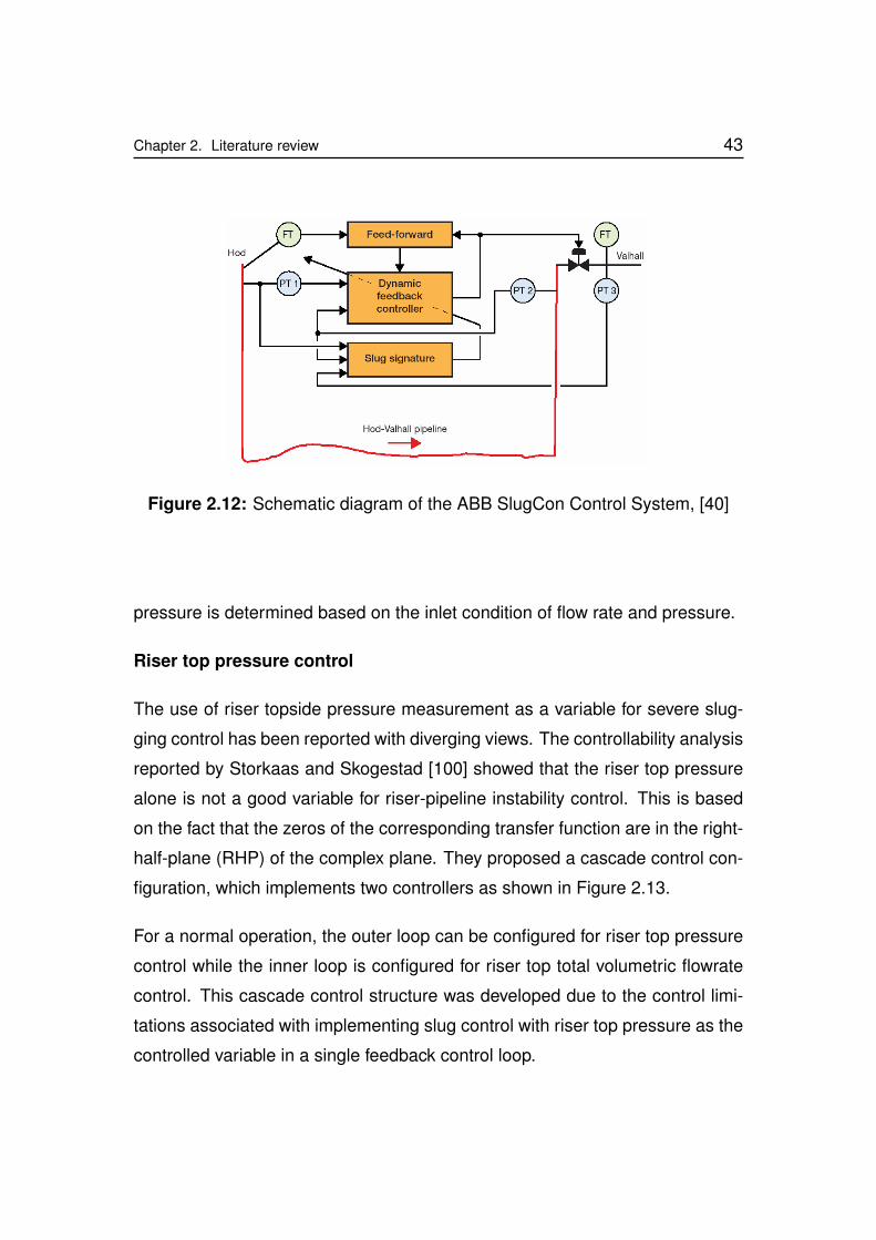
Chapter 2. Literature review 43
Figure 2.12: Schematic diagram of the ABB SlugCon Control System, [40]
pressure is determined based on the inlet condition of flow rate and pressure.
Riser top pressure control
The use of riser topside pressure measurement as a variable for severe slug-
ging control has been reported with diverging views. The controllability analysis
reported by Storkaas and Skogestad [100] showed that the riser top pressure
alone is not a good variable for riser-pipeline instability control. This is based
on the fact that the zeros of the corresponding transfer function are in the right-
half-plane (RHP) of the complex plane. They proposed a cascade control con-
figuration, which implements two controllers as shown in Figure 2.13.
For a normal operation, the outer loop can be configured for riser top pressure
control while the inner loop is configured for riser top total volumetric flowrate
control. This cascade control structure was developed due to the control limi-
tations associated with implementing slug control with riser top pressure as the
controlled variable in a single feedback control loop.
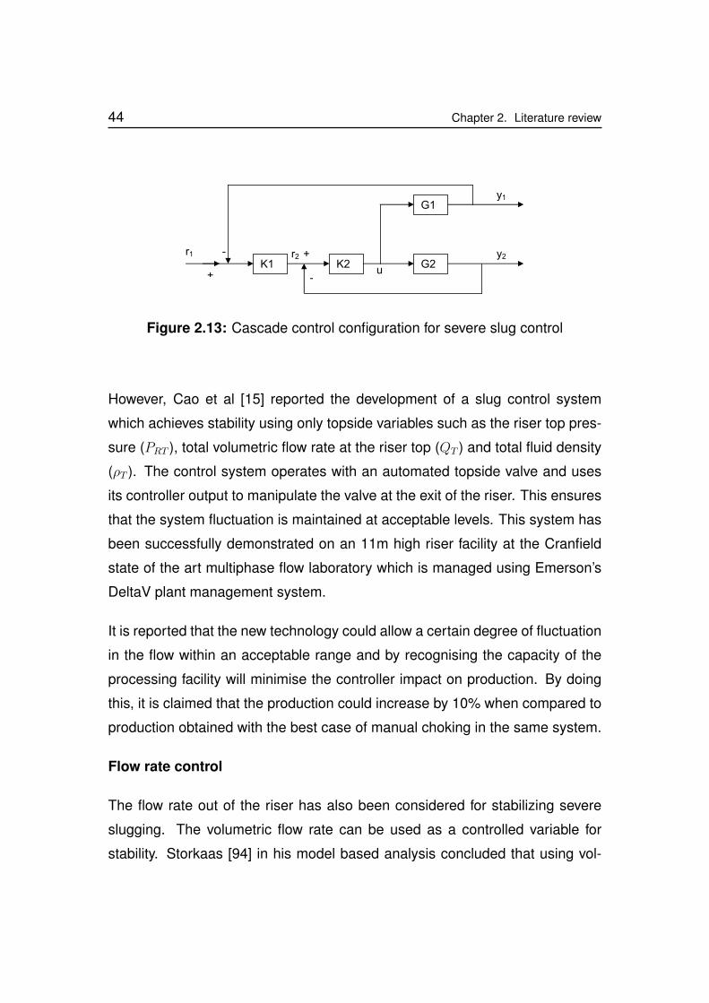
44 Chapter 2. Literature review
K1 K2 G2
G1
r1 -
+
r2 +
-u
y1
y2
Figure 2.13: Cascade control configuration for severe slug control
However, Cao et al [15] reported the development of a slug control system
which achieves stability using only topside variables such as the riser top pres-
sure (PRT ), total volumetric flow rate at the riser top (QT ) and total fluid density
(ρT ). The control system operates with an automated topside valve and uses
its controller output to manipulate the valve at the exit of the riser. This ensures
that the system fluctuation is maintained at acceptable levels. This system has
been successfully demonstrated on an 11m high riser facility at the Cranfield
state of the art multiphase flow laboratory which is managed using Emerson’s
DeltaV plant management system.
It is reported that the new technology could allow a certain degree of fluctuation
in the flow within an acceptable range and by recognising the capacity of the
processing facility will minimise the controller impact on production. By doing
this, it is claimed that the production could increase by 10% when compared to
production obtained with the best case of manual choking in the same system.
Flow rate control
The flow rate out of the riser has also been considered for stabilizing severe
slugging. The volumetric flow rate can be used as a controlled variable for
stability. Storkaas [94] in his model based analysis concluded that using vol-

Chapter 2. Literature review 45
umetric flow rate as a controlled variable will give poor performance at low
frequency. He also concluded that using volumetric flow rate in the inner loop
of a cascade control design to control the flowrate out of the riser could give
better performance. An improved slug catcher designed with dynamic choking
and intelligent control system can be used to suppress severe slugging through
flowrate control, as reported by Kovalev et al [57, 58] (see Figure 2.14).
Control
System
P
L
F
F
First Stage
Separator
Mini-
separator
S3
Inlet Flow line
Figure 2.14: Schematic diagram of the S3 control scheme
The slug suppression system (S3) control strategy is based on total volumetric
flow control and liquid flow control [57]. The measured variables include the
liquid and gas volumetric flowrates, the separator pressure and separator liquid
level, while the controlled variable is the total volumetric flowrate (the sum of
the gas and liquid volumetric flowrate measured separately using flow meters).
Under severe slugging conditions, the total volumetric flowrate control mode
is not implemented, rather the liquid flow control mode operates to slow down
slug velocity and prevent slug blow-out.
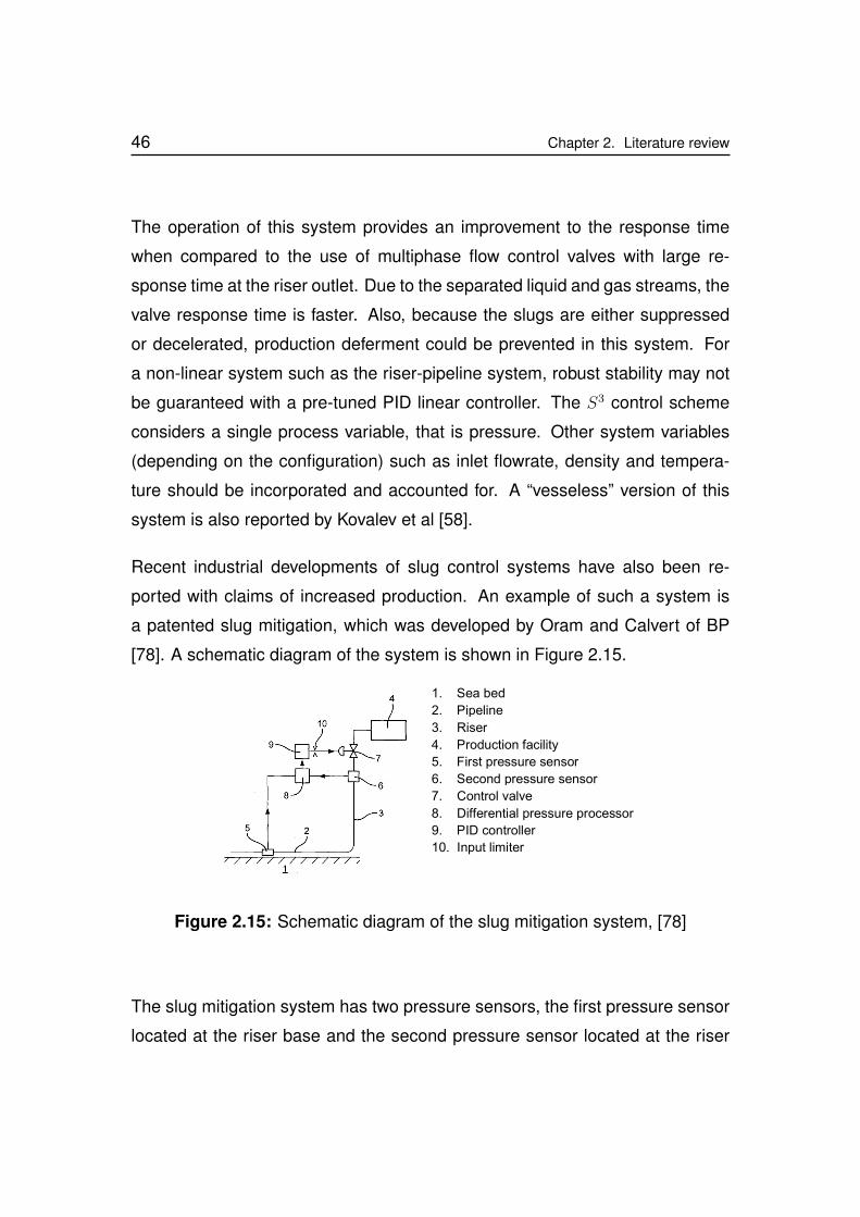
46 Chapter 2. Literature review
The operation of this system provides an improvement to the response time
when compared to the use of multiphase flow control valves with large re-
sponse time at the riser outlet. Due to the separated liquid and gas streams, the
valve response time is faster. Also, because the slugs are either suppressed
or decelerated, production deferment could be prevented in this system. For
a non-linear system such as the riser-pipeline system, robust stability may not
be guaranteed with a pre-tuned PID linear controller. The S3 control scheme
considers a single process variable, that is pressure. Other system variables
(depending on the configuration) such as inlet flowrate, density and tempera-
ture should be incorporated and accounted for. A “vesseless” version of this
system is also reported by Kovalev et al [58].
Recent industrial developments of slug control systems have also been re-
ported with claims of increased production. An example of such a system is
a patented slug mitigation, which was developed by Oram and Calvert of BP
[78]. A schematic diagram of the system is shown in Figure 2.15.
1. Sea bed
2. Pipeline
3. Riser
4. Production facility
5. First pressure sensor
6. Second pressure sensor
7. Control valve
8. Differential pressure processor
9. PID controller
10. Input limiter
Figure 2.15: Schematic diagram of the slug mitigation system, [78]
The slug mitigation system has two pressure sensors, the first pressure sensor
located at the riser base and the second pressure sensor located at the riser

Chapter 2. Literature review 47
top. The pressure difference between the two pressure sensors is processed
by the differential pressure processor. Thus, the controller input is the differen-
tial pressure. The slug controller is a traditional PID controller whose integral
time is set equal to zero, resulting to a PD controller. The controller output ma-
nipulates the control valve, whose upper and lower limit is set to about ±20%
of its nominal value, to mitigate the severe slugging in the system. The dif-
ferential pressure set point is determined by the operator. In another version
of the system, a master PI controller with large integral time and small gain is
used to automatically set the set point for the PD controller. The PD controller
is considered as a slave, while the PI controller is considered as the master
controller. The input to the master controller is pressure measurement from the
first pressure (sea bed) sensor. The operator determines the pressure set point
of the PI controller. Another version of the system is also presented, in which a
dynamic valve constraint control is implemented. To achieve the dynamic con-
straint control, the upper and lower limits of the control valve is determined and
set automatically from the process history. It is reported that the implementa-
tion of this slug control system on the Valhall production platform off the coast
of Norway was successful, with claims that the slug control system increased
production by 10% [14].
2.5 Conclusions
In conclusion, this chapter has presented a review of the severe slug control
techniques, including their applications, limitations and challenges. Various
forms of severe slug control techniques including modifying internal pipeline
diameter, riser base gas injection, pipeline gas re-injection and manual and
active choking of the riser top vales has been discussed. It can be deduced
48 Chapter 2. Literature review
that vast amount of work has been done to develop systems for severe slug
control. However, the lack of adequate information on the performance of these
systems is a challenge to deciding the direction for their further development.
The conflicting report on the performance of similar techniques exposes the
gap in the available knowledge of severe slug control. Thus, extensive amount
of work is still required in order to gain sufficient knowledge and understanding
of severe control and the sharing of available information could be the key to its
success.
Chapter 3
Experimental facilities and
procedure
3.1 Introduction
This chapter explains the experimental facilities and procedures used in the
conduct of the experiment and in the acquisition of experimental data gener-
ated in the experiment. The experimental facility, which is located in the flow
laboratory of the department of Process and Systems Engineering in Cranfield
University consists of standard multiphase flow test rigs, including the riser-
pipeline systems used in this work. The experimental facility is designed to
continuously and safely process multiphase fluid under different operating con-
ditions at real time. The chapter begins with the description of the multiphase
flow facility and the operating conditions. The description of the different sec-
tions used for processing the flow in and out of the riser systems is also pre-
sented.
Also explained in this chapter is an industrial riser system, which is of a larger
scale, when compared to the experimental facility. The industrial riser system
49
50 Chapter 3. Experimental facilities and procedure
is not a physical experimental system, but a model based riser system, which
is of industrial dimension. Thanks to the Scan Power Technology (SPT) Group
for providing this system.
3.2 The multiphase flow facility
The multiphase flow test facility can be divided into three main sections. These
include:
1. fluid supply and metering section
2. test section
3. phase separation section
The schematic diagram of the facility is shown in Figure 3.1.
3.2.1 Fluid supply and metering section
The fluid supply and metering section is the section that safely stores, supplies
and provide measurement for the single phase fluid used in all the experiments.
It is divided into three independent sources, each containing a single phase
fluid. These include, air, water and oil sources. These three supply sources are
discussed below.
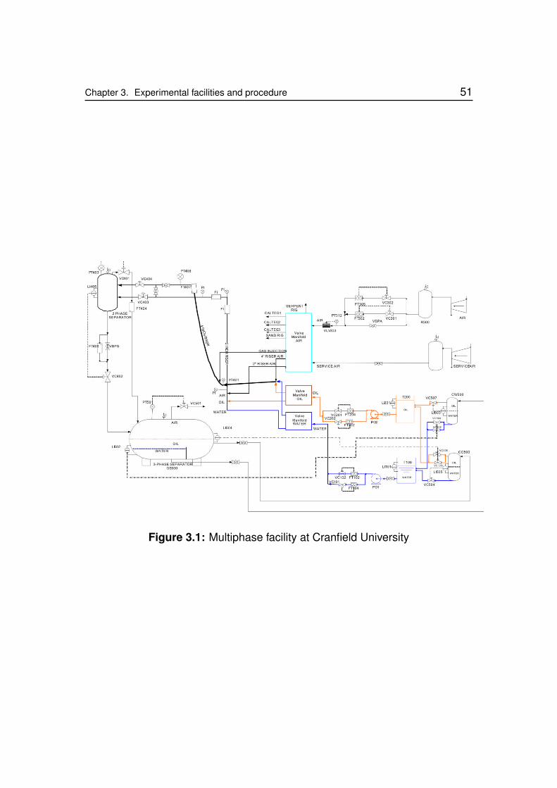
Chapter 3. Experimental facilities and procedure 51
Figure 3.1: Multiphase facility at Cranfield University
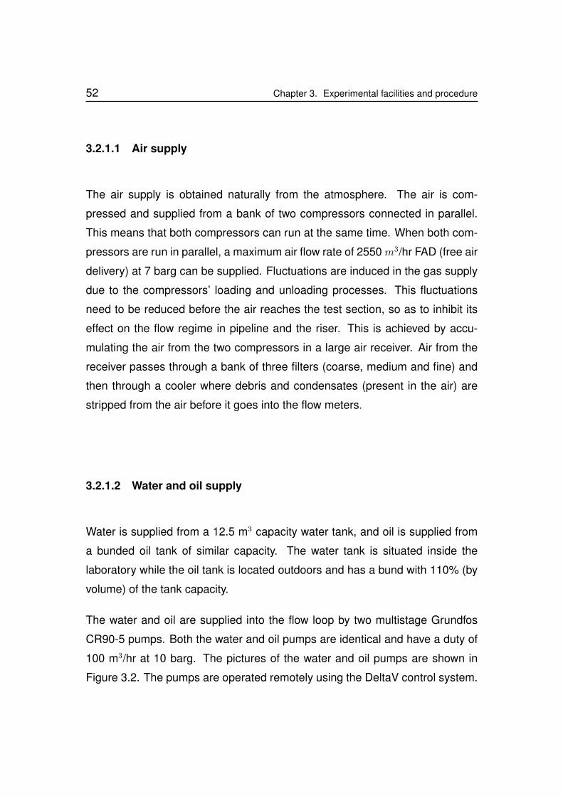
52 Chapter 3. Experimental facilities and procedure
3.2.1.1 Air supply
The air supply is obtained naturally from the atmosphere. The air is com-
pressed and supplied from a bank of two compressors connected in parallel.
This means that both compressors can run at the same time. When both com-
pressors are run in parallel, a maximum air flow rate of 2550 m3/hr FAD (free air
delivery) at 7 barg can be supplied. Fluctuations are induced in the gas supply
due to the compressors’ loading and unloading processes. This fluctuations
need to be reduced before the air reaches the test section, so as to inhibit its
effect on the flow regime in pipeline and the riser. This is achieved by accu-
mulating the air from the two compressors in a large air receiver. Air from the
receiver passes through a bank of three filters (coarse, medium and fine) and
then through a cooler where debris and condensates (present in the air) are
stripped from the air before it goes into the flow meters.
3.2.1.2 Water and oil supply
Water is supplied from a 12.5 m3 capacity water tank, and oil is supplied from
a bunded oil tank of similar capacity. The water tank is situated inside the
laboratory while the oil tank is located outdoors and has a bund with 110% (by
volume) of the tank capacity.
The water and oil are supplied into the flow loop by two multistage Grundfos
CR90-5 pumps. Both the water and oil pumps are identical and have a duty of
100 m3/hr at 10 barg. The pictures of the water and oil pumps are shown in
Figure 3.2. The pumps are operated remotely using the DeltaV control system.
Chapter 3. Experimental facilities and procedure 53
(a) Water pump (b) Oil pump
Figure 3.2: Water and oil pumps
In the water supply loop, there are two metering lines each comprising a con-
trol valve and a flow meter, which provides metering for the flow from 0-7.36
kg/s and 0-30 kg/s, respectively. The DeltaV system will accurately select the
appropriate water metering flow loop when the desired flow rate is specified.
In the oil supply loop, there are also two metering lines, each comprising a
control valve and a flow meter, which provides metering for the flow of 0-9.47
kg/s and 0-30 kg/s, respectively.
3.2.1.3 Flow metering
The flow rates of the air, water and oil are regulated using their respective con-
trol valves. These control valves are controlled by the supervisory control and
data acquisition (SCADA) software, DeltaV. The water flow rate is measured by
a 1 inch Rosemount 8742 Magnetic flow meter (up to 1 kg/s) and 3 inch Foxboro
CFT50 Coriolis meter (up to 10 kg/s) while the oil flow rate is measured by a
54 Chapter 3. Experimental facilities and procedure
1 inch Micro Motion Mass flow meter (up to 1 kg/s) and 3 inch Foxboro CFT50
Coriolis meter (up to 10 kg/s). The air is metered by a bank of two Rosemount
Mass Probar flow meters of 0.5 inch and 1 inch diameter respectively. The
smaller air flow meter measures the lower air flow rate (up to 120 Sm3/h) while
the larger one meters the higher air flow rate up to 4250 Sm3/h (subject to
compressor capacity).
3.2.2 The test section
Fluid supplied from the fluid supply section flows into the test section. The
test section comprises of the riser systems, the two phase separator and the
accompanying measuring instruments. There are two riser systems, which can
run alternatively. The two riser systems are:
1. a 4 inch riser system and
2. a 2 inch riser system.
3.2.2.1 The 4 inch riser system
The 4 inch riser is a catenary riser with upstream pipeline length of 55m, which
is inclined downwardly at 2◦. The riser height is also about 10.5m. The up-
stream pipeline connects to the riser at the riser base. Fluid supply for the 4
inch riser system comes from the three independent single-phase sources for
oil (dielectric 250), water and air. The supplied fluid mixes at a mixing point
before flowing into the 55m pipeline, which connects to the riser at the base.
A pressure transmitter, which is labeled PT401 in Figure 3.1 is installed at the
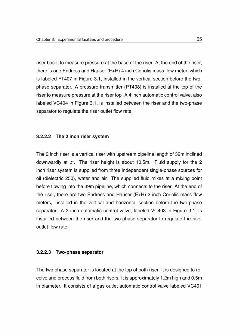
Chapter 3. Experimental facilities and procedure 55
riser base, to measure pressure at the base of the riser. At the end of the riser,
there is one Endress and Hauser (E+H) 4 inch Coriolis mass flow meter, which
is labeled FT407 in Figure 3.1, installed in the vertical section before the two-
phase separator. A pressure transmitter (PT408) is installed at the top of the
riser to measure pressure at the riser top. A 4 inch automatic control valve, also
labeled VC404 in Figure 3.1, is installed between the riser and the two-phase
separator to regulate the riser outlet flow rate.
3.2.2.2 The 2 inch riser system
The 2 inch riser is a vertical riser with upstream pipeline length of 39m inclined
downwardly at 2◦. The riser height is about 10.5m. Fluid supply for the 2
inch riser system is supplied from three independent single-phase sources for
oil (dielectric 250), water and air. The supplied fluid mixes at a mixing point
before flowing into the 39m pipeline, which connects to the riser. At the end of
the riser, there are two Endress and Hauser (E+H) 2 inch Coriolis mass flow
meters, installed in the vertical and horizontal section before the two-phase
separator. A 2 inch automatic control valve, labeled VC403 in Figure 3.1, is
installed between the riser and the two-phase separator to regulate the riser
outlet flow rate.
3.2.2.3 Two-phase separator
The two phase separator is located at the top of both riser. It is designed to re-
ceive and process fluid from both risers. It is approximately 1.2m high and 0.5m
in diameter. It consists of a gas outlet automatic control valve labeled VC401
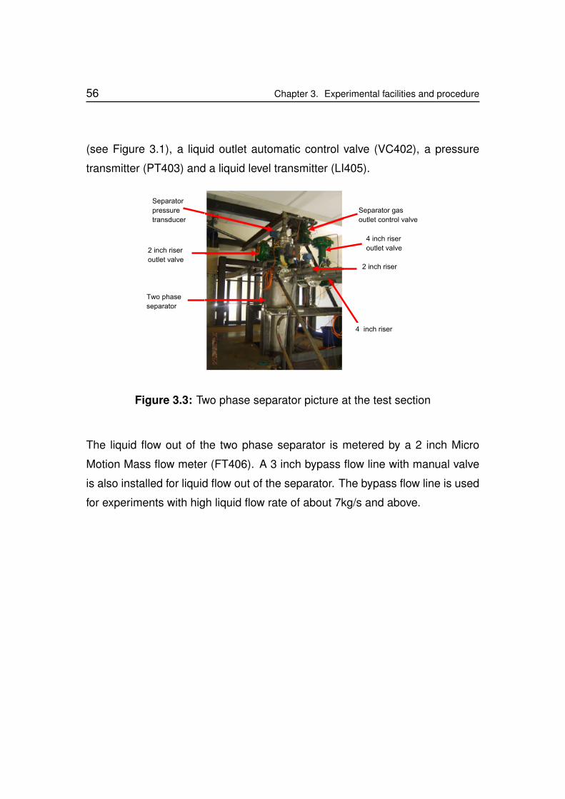
56 Chapter 3. Experimental facilities and procedure
(see Figure 3.1), a liquid outlet automatic control valve (VC402), a pressure
transmitter (PT403) and a liquid level transmitter (LI405).
Two phase
separator
2 inch riser
4 inch riser
Separator gas
outlet control valve
2 inch riser
outlet valve
Separator
pressure
transducer
4 inch riser
outlet valve
Figure 3.3: Two phase separator picture at the test section
The liquid flow out of the two phase separator is metered by a 2 inch Micro
Motion Mass flow meter (FT406). A 3 inch bypass flow line with manual valve
is also installed for liquid flow out of the separator. The bypass flow line is used
for experiments with high liquid flow rate of about 7kg/s and above.
Chapter 3. Experimental facilities and procedure 57
3.2.3 Phase separation section
The phase separation section receives the liquid and gas from the two phase
separator. This section comprises of a 3-phase separator and two coalescers.
3.2.3.1 The three-phase separator
Gravity separation of the three phase flow into their single phases of oil, wa-
ter and air is achieved in the three-phase separator. There are three sets of
controllers, namely, pressure controller, oil-water interface level controller and
gas-liquid level controller. The oil/water interface level is controlled by manip-
ulating the control valves labeled VC502 and VC503 (see Figure 3.1), using a
Split Range Control Module. For low flow rate out of the separator, the VC502
is used while for high flow rate VC503 is used. Also, the air/oil interface level is
controlled by manipulating the control valves labeled VC505 and VC506, using
a Split Range Control Module. For low flow rate out of the separator, the VC505
is used while for high flow rate VC506 is used. The oil and water released
from the 3-phase separator flows in to the oil-water coalescer. The oil-water
coalescer is used to achieve a more efficient separation of the oil and water
phases. There are two coalescers. Each coalescer has an oil-water level con-
troller. The oil and water released from the coalescers flow into their respective
storage tanks.

58 Chapter 3. Experimental facilities and procedure
3.3 Running the experiments
To run the experiment, firstly the manual control valves at the valve manifold
are positioned in the right order for the riser system required for the experi-
ment. This is very necessary to ensure that the liquid and gas flow through
the required riser system safely. The compressor is then powered ON. The
liquid pump is powered ON and controlled through the DeltaV control system.
The desired liquid and air flow rates are set in the DeltaV flow metering envi-
ronment. Each set flowrate is controlled to the set value by the DeltaV control
system. The experimental data is obtained through the data acquisition system
(see section 3.4).
3.3.1 Operating condition
Before commencing each experiment, the operating condition of the experi-
mental facility is set to a suitable condition to ensure that the system can gen-
erate the required severe slugging flow regime. This is achieved by monitoring
the system through the DeltaV system. The outlet pressure of the three phase
separator is controlled at 1 barg for all the experiments. The temperature varies
between 22oC to 25oC during the experiments. The liquid and air flow rate is
controlled by the supervisory control and data acquisition (SCADA) software,
DeltaV.
Chapter 3. Experimental facilities and procedure 59
3.4 Data acquisition system
The multiphase test facility is controlled by a supervisory control and data ac-
quisition (SCADA) software, DeltaV. This software is supplied by Emerson Pro-
cess Management. The process data from the measuring instruments are con-
nected to the DeltaV system in the control room. All pressure controllers, flow
controllers, level controllers and safety interlocks are maintained and controlled
by the DeltaV. The sampling rate of all the signals managed by DeltaV system is
at 1 Hz rate. The recorded signals are stored in the DeltaV Historian database.
The data can be downloaded from the DeltaV system for each variable after the
experimental period.
3.5 Industrial riser system
The industrial riser system is an 8 inch riser-pipeline system consisting of
a 5000m long pipeline, a 120m high riser and a pressure driven well of 69
barg. The reservoir temperature is 70oC and the its production index is 10.12
Sm3/d/bar (4.4 SBbl/d/psi). An additional gas lift source with a constant mass
flowrate is applied to the well-head. The riser top has an 8 inch valve at the
outlet. The schematic diagram of the generic riser system is shown in Figure
3.4. The industrial riser system is modelled using the commercial multiphase
flow simulator OLGA, and the improved simplified riser model (ISRM). The de-
velopment of the ISRM will be discussed in Chapter 4.
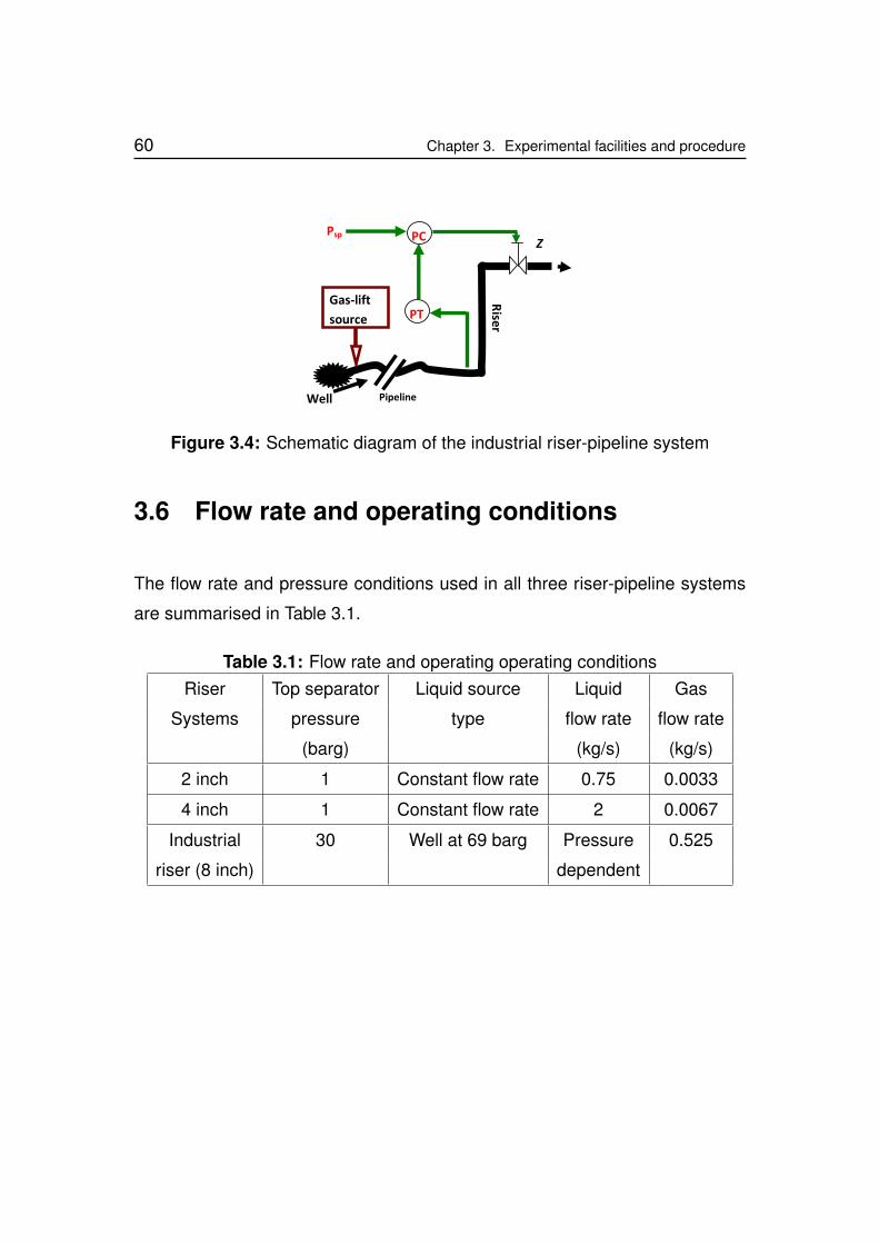
60 Chapter 3. Experimental facilities and procedure
Well
Riser
Pipeline
Gas-lift
source PT
PCPspZ
Figure 3.4: Schematic diagram of the industrial riser-pipeline system
3.6 Flow rate and operating conditions
The flow rate and pressure conditions used in all three riser-pipeline systems
are summarised in Table 3.1.
Table 3.1: Flow rate and operating operating conditionsRiser Top separator Liquid source Liquid Gas
Systems pressure type flow rate flow rate
(barg) (kg/s) (kg/s)
2 inch 1 Constant flow rate 0.75 0.0033
4 inch 1 Constant flow rate 2 0.0067
Industrial 30 Well at 69 barg Pressure 0.525
riser (8 inch) dependent
Chapter 4
Plant-wide modeling for severe
slugging prediction and control
4.1 Introduction
In this chapter, the modeling of the major system units of the riser-pipeline
system for severe slug flow prediction and control performance analysis is dis-
cussed. In order to study the non-linear characteristics of severe slugging and
design a robust control system for its suppression, a reliable model of the riser-
pipeline system is required. Such a model should be able to predict the non
linear characteristics of the severe slug flow. With slug control design in mind,
such a model should, in addition to predicting severe slugging, be able to pre-
dict control performances required for slug controller design. Thus, a model
that would be relevant for gaining the fundamental understanding of the severe
slug control would be one that has the ability to:
1. predict severe slugging
2. estimate control performance
61
62 Chapter 4. Plant-wide modeling for severe slugging prediction and control
In order to ensure that the predicted flow characteristics are reliable and repre-
sents the real system behaviour, the modeling of the major system units of the
riser-pipeline production system will be required.
4.2 Plant-wide model
In line with the objectives of this project, which is to study severe slugging con-
trol in a plant-wide scale, the modeling of the major system units of the riser
production system and their performances is discussed in this section. The
severe slug predicting model, which contains the models of the major system
units of the riser-pipeline production system is known as a plant-wide model.
To develop the plant-wide model, these major system units namely: the riser-
pipeline, the topside separator and the pressure driven fluid source are mod-
elled and linked together. Experimental studies have shown that the interaction
between the process variables in these systems, such as pressure, affect the
ability to control severe slugging [116].
4.2.1 The riser-pipeline model
The riser-pipeline model is a very important part of the plant-wide model. One
major condition for the occurrence of severe slugging is the inclination of the
pipeline, upstream of the riser inlet. A number of severe slug models have been
developed using only the pipeline and the riser as a single unit [6, 67, 103]. The
challenge with these models is their ability to accurately predict the nonlinear
characteristics of severe slugging and the control performances of the system
Chapter 4. Plant-wide modeling for severe slugging prediction and control 63
without complex and unrealistic mathematical solutions. The suitability of some
riser-pipeline models for severe slug control design will be briefly discussed.
4.2.1.1 Suitability of riser-pipeline models
A reliable slug controller is required for the study and the analysis of the control
performance of the slug control system. In order to design a model based
slug controller, a linearised model is normally desired. The linearisation of a
nonlinear model requires that the internal equations of the nonlinear model
should be readily accessible, and that the linearisation should be performed
with the existing tools and methods. The two fluid model, the drift flux model
and commercial multiphase flow simulators such as the OLGA models, are
some of the exisiting models, which can predict severe slugging. However,
there are some challenges with the application of these models in slug control
design and performance analysis.
The two fluid model is based on mass and momentum balance for each phase
while the drift flux model applies mass balance equation for each phase and
a combined momentum balance for all the phases [46]. Both models are ex-
pressed in partial differential equations (PDEs) [102]. To obtain a model in
ordinary differential equations (ODEs) for control design, the PDE model has
to be transformed by space discretisation. However, the order of the model
obtained from this process can be very high such that the numerical optimisa-
tion required for model based controller design gets complicated. This limits
the application of both PDE models in model based design for severe slugging
control. A model based on commercial simulators such as OLGA, cannot pro-
vide readily accessible internal equations due to commercial reasons, making
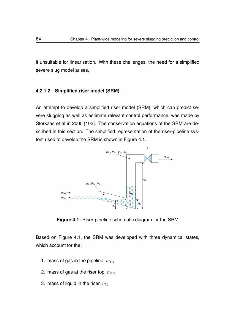
64 Chapter 4. Plant-wide modeling for severe slugging prediction and control
it unsuitable for linearisation. With these challenges, the need for a simplified
severe slug model arises.
4.2.1.2 Simplified riser model (SRM)
An attempt to develop a simplified riser model (SRM), which can predict se-
vere slugging as well as estimate relevant control performance, was made by
Storkaas et al in 2005 [102]. The conservation equations of the SRM are de-
scribed in this section. The simplified representation of the riser-pipeline sys-
tem used to develop the SRM is shown in Figure 4.1.
θh1
HR
mLin
mGin
H1
mG1, PRB, VG1
mG2, PRT, VG2, αLT
mL
u
mmix
Figure 4.1: Riser-pipeline schematic diagram for the SRM
Based on Figure 4.1, the SRM was developed with three dynamical states,
which account for the:
1. mass of gas in the pipeline, mG1
2. mass of gas at the riser top, mG2
3. mass of liquid in the riser, mL
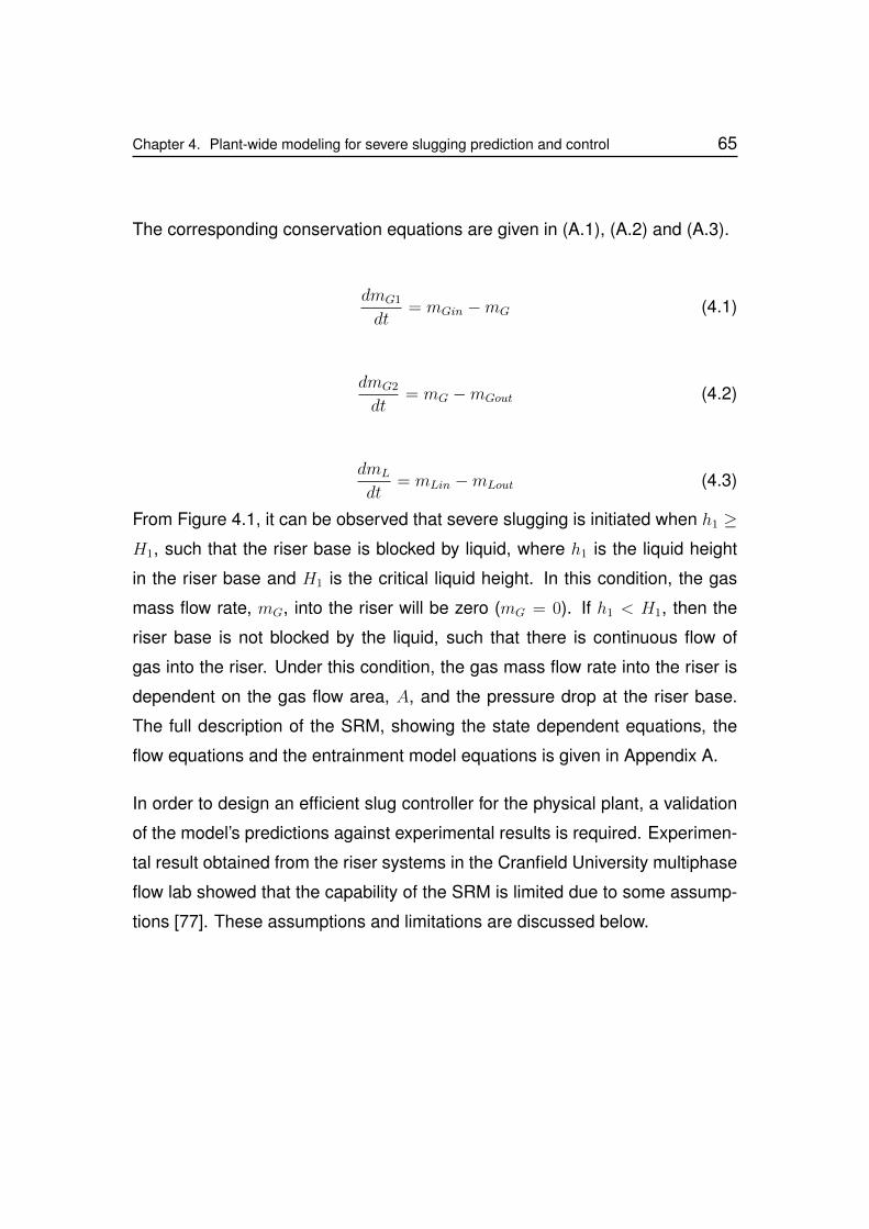
Chapter 4. Plant-wide modeling for severe slugging prediction and control 65
The corresponding conservation equations are given in (A.1), (A.2) and (A.3).
dmG1
dt= mGin −mG (4.1)
dmG2
dt= mG −mGout (4.2)
dmL
dt= mLin −mLout (4.3)
From Figure 4.1, it can be observed that severe slugging is initiated when h1 ≥H1, such that the riser base is blocked by liquid, where h1 is the liquid height
in the riser base and H1 is the critical liquid height. In this condition, the gas
mass flow rate, mG, into the riser will be zero (mG = 0). If h1 < H1, then the
riser base is not blocked by the liquid, such that there is continuous flow of
gas into the riser. Under this condition, the gas mass flow rate into the riser is
dependent on the gas flow area, A, and the pressure drop at the riser base.
The full description of the SRM, showing the state dependent equations, the
flow equations and the entrainment model equations is given in Appendix A.
In order to design an efficient slug controller for the physical plant, a validation
of the model’s predictions against experimental results is required. Experimen-
tal result obtained from the riser systems in the Cranfield University multiphase
flow lab showed that the capability of the SRM is limited due to some assump-
tions [77]. These assumptions and limitations are discussed below.
66 Chapter 4. Plant-wide modeling for severe slugging prediction and control
Limitations of the SRM
The assumptions that limit the performance of the SRM are highlighted below:
1. The riser outlet pressure (separator pressure), Ps, is assumed to be con-
stant, which effectively means a separator with an infinite volume con-
nected at the riser outlet. This does not represent any real system as
the dynamics of the topside processing equipment (the separator) has a
significant effect on the severe slugging behaviour as was demonstrated
in previous work by Yeung et al [116].
2. The model does not account for the slug production stage, which occur in
the severe slug cycle. The omission of this stage affects the prediction of
liquid flow pattern out of the riser, and limits the application of the model
in analysing the accumulated production over a production period, during
severe slugging.
3. The assumption of constant pipeline gas volume (VG1) in the pipeline,
which implies constant liquid hold up, limits the prediction of the slug am-
plitude and frequency accurately simultaneously. According to Storkaas
(2005, pp 47), “..the simplified three state model predicts a slug frequency
that, compared to the OLGA simulations, is about 10-20% too high for low-
to-medium range valve openings and up to about 50% too high for large
valve openings. The higher frequency probably comes from neglecting
the liquid dynamics in the feed section. ...and when the upstream gas
volume is fixed, we cannot achieve both frequency and amplitude simul-
taneously”. Consequently, the model only offers the choice of predicting
accurate slug amplitude or frequency at a time, not both.
4. The model assumes fixed liquid and gas inlet flow rates. Any change to
the inlet flow rates will require re-tuning the model parameters. Therefore,
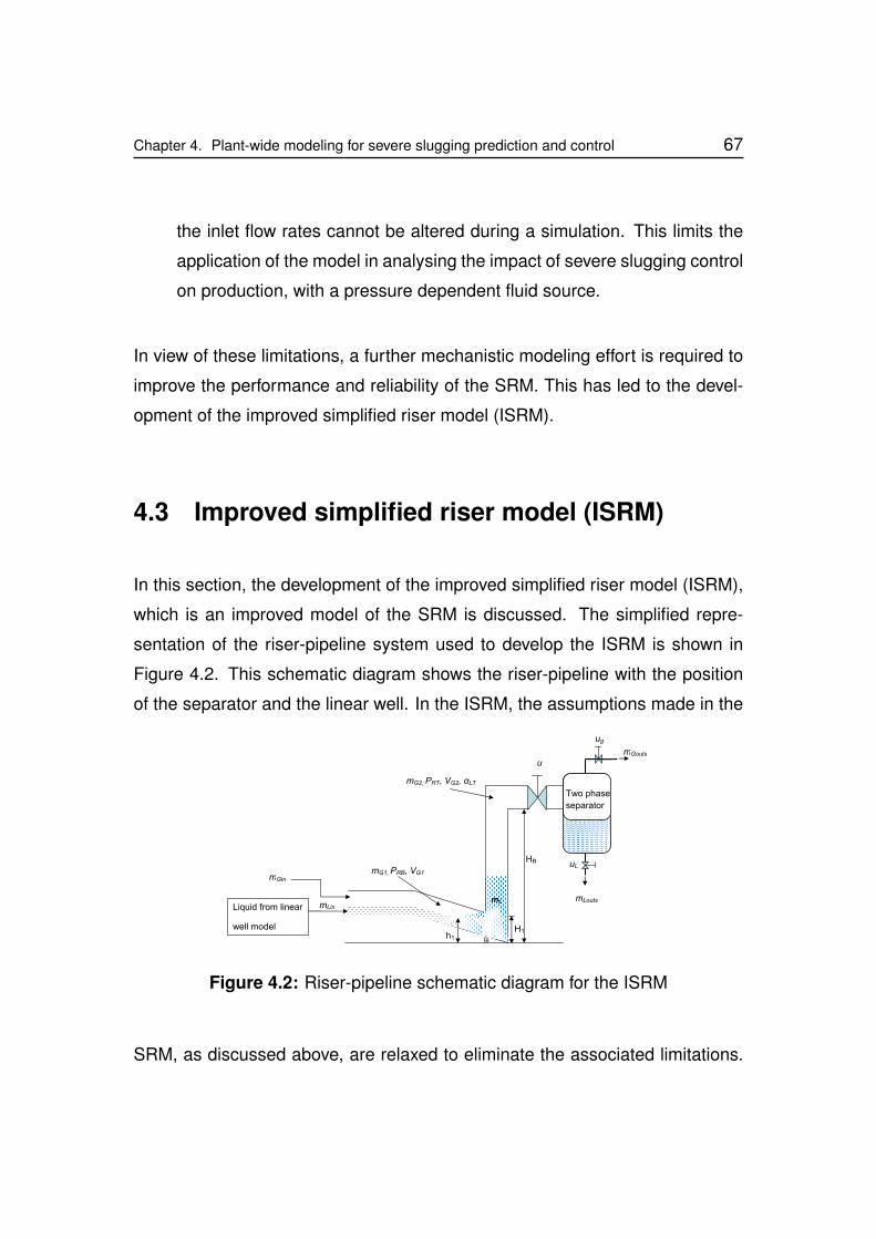
Chapter 4. Plant-wide modeling for severe slugging prediction and control 67
the inlet flow rates cannot be altered during a simulation. This limits the
application of the model in analysing the impact of severe slugging control
on production, with a pressure dependent fluid source.
In view of these limitations, a further mechanistic modeling effort is required to
improve the performance and reliability of the SRM. This has led to the devel-
opment of the improved simplified riser model (ISRM).
4.3 Improved simplified riser model (ISRM)
In this section, the development of the improved simplified riser model (ISRM),
which is an improved model of the SRM is discussed. The simplified repre-
sentation of the riser-pipeline system used to develop the ISRM is shown in
Figure 4.2. This schematic diagram shows the riser-pipeline with the position
of the separator and the linear well. In the ISRM, the assumptions made in the
θ h1
HR
H1
mG1, PRB, VG1
mG2, PRT, VG2, αLT
mL
u
ug
uLu
Liquid from linear
well model
mGin
mLin
Two phase
separator
mLouts
mGouts
Figure 4.2: Riser-pipeline schematic diagram for the ISRM
SRM, as discussed above, are relaxed to eliminate the associated limitations.
68 Chapter 4. Plant-wide modeling for severe slugging prediction and control
The upstream gas volume, which is assumed constant in the SRM is modelled
as a function of the dynamic pipeline pressure and fluid inlet flow rates, while
the accumulated liquid upstream the riser inlet is modelled to enhance the pre-
diction of the slug production stage. In addition, a topside two phase separator
model and a linear well model are developed and linked to the ISRM to make
up the ISRM with well and separator model.
4.3.1 Conservation equations of the ISRM
The ISRM consists of five dynamical state equations which account for:
1. mass of gas in the pipeline, mG1
2. mass of gas at the riser top, mG2
3. mass of liquid in the riser, mL
4. separator top pressure, Ps
5. separator liquid height, hL
The corresponding conservation equations for the mG1, mG2 and the mL are
given in (4.4), (4.5) and (4.6) respectively.
dmG1
dt= mGin −mG (4.4)
dmG2
dt= mG −mGout (4.5)

Chapter 4. Plant-wide modeling for severe slugging prediction and control 69
dmL
dt= mLin −mLout (4.6)
The conservation equations for the Ps and the hL, which are given in (4.7) and
(4.8) result from the modeling of the two-phase separator to achieve dynamic
riser outlet boundary condition. This eliminates the constant outlet boundary
condition in the SRM. The two-phase separator modeling is presented in sec-
tion 4.3.1.1.
dPsdt
=Ps
As(Hs − hL)
[(QGins −QGouts) + As
dhLdt
](4.7)
In 4.7, As is the separator cross sectional area, Hs is the separator height and
hL is the liquid level in the separator, QGins is the gas volume flow rate into the
separator, and QGouts is the gas volume flow rate out of the separator.
dhLdt
=mLins −mLouts
AsρL(4.8)
In 4.8, mLins is the liquid mass flow rate into the separator, and mLouts is the
liquid mass flow rate out of the separator.
4.3.1.1 Dynamic riser outlet boundary condition - the separator model
In the SRM, the riser outlet pressure is assumed to be constant, which effec-
tively means a separator with an infinite volume connected at the riser outlet.
Thus, the dynamic effect of the topside separator on the performance, stability
and productivity of the system is neglected. This will affect the ability of the
model to accurately predict severe slugging and estimate control performances
reliably. To eliminate this condition, a two phase separator model is developed
to replace the constant pressure condition at the riser outlet. The schematic
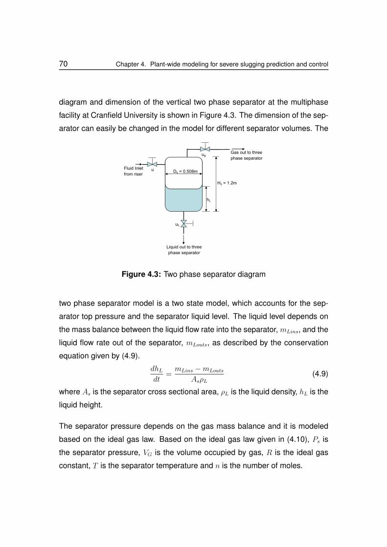
70 Chapter 4. Plant-wide modeling for severe slugging prediction and control
diagram and dimension of the vertical two phase separator at the multiphase
facility at Cranfield University is shown in Figure 4.3. The dimension of the sep-
arator can easily be changed in the model for different separator volumes. The
ug
Liquid out to three
phase separator
hL
Hs = 1.2m
Gas out to three
phase separator
uL
Ds = 0.508muFluid Inlet
from riser
Figure 4.3: Two phase separator diagram
two phase separator model is a two state model, which accounts for the sep-
arator top pressure and the separator liquid level. The liquid level depends on
the mass balance between the liquid flow rate into the separator, mLins, and the
liquid flow rate out of the separator, mLouts, as described by the conservation
equation given by (4.9).
dhLdt
=mLins −mLouts
AsρL(4.9)
where As is the separator cross sectional area, ρL is the liquid density, hL is the
liquid height.
The separator pressure depends on the gas mass balance and it is modeled
based on the ideal gas law. Based on the ideal gas law given in (4.10), Ps is
the separator pressure, VG is the volume occupied by gas, R is the ideal gas
constant, T is the separator temperature and n is the number of moles.
Chapter 4. Plant-wide modeling for severe slugging prediction and control 71
PsVG = nRT (4.10)
The volume occupied by the gas VG is given by:
VG = As(Hs − hL) (4.11)
By taking the partial differential of (4.10), (4.12) is obtained.
PsdVGdt
+ VGdPsdt
= RTdn
dt(4.12)
The number of moles, n, is given by (4.13),
n =m
M(4.13)
where m is the mass of gas in the separator and M is the molecular weight of
the gas. By, substituting (4.13) into (4.12), (4.14) is obtained,
PsdVGdt
+ VGdPsdt
=RT
M
dm
dt(4.14)
anddm
dt= mGins −mGouts (4.15)
where mGins is the gas mass flow rate of gas into the separator, and mGouts is
the gas mass flow rate out of the separator. It is assumed that the pressure
in the pipeline at the separator inlet will be approximately the same with the
separator pressure. Thus, expressing (4.15) in terms of volumetric flow rate,
(4.16) is obtained,dm
dt= ρGs(QGins −QGouts) (4.16)
where ρGs is the density of gas in the separator. By substituting (4.16) into
(4.14), (4.17) is obtained.
PsdVGdt
+ VGdPsdt
= Ps(QGins −QGouts) (4.17)
72 Chapter 4. Plant-wide modeling for severe slugging prediction and control
By substituting (4.11) into (4.17), (4.18) is obtained.
PsAsd(Hs − hL)
dt+ As(Hs − hL)
dPsdt
= Ps(QGins −QGouts) (4.18)
Rearranging (4.18) for dPsdt
, the dynamic equation for the separator pressure is
obtained as given in (4.19).
dPsdt
=Ps
As(Hs − hL)
[(QGins −QGouts) + As
dhLdt
](4.19)
4.3.2 State dependent variables
The state dependent variables such as the riser base pressure, PRB, and riser
top pressure, PRT , are calculated using the ideal gas law, and are given by
(4.20) and (4.21), where VG1 is the volume of gas in the pipeline, VG1, and VG2
is the volume of gas at the riser top.
PRB =mG1RT
VG1MG
(4.20)
PRT =mG2RT
VG2MG
(4.21)
The volume of gas in the pipeline, VG1, which was assumed constant in the
SRM is modeled in the ISRM to achieve dynamic update of its value based on
the flow rate into the pipeline.
Chapter 4. Plant-wide modeling for severe slugging prediction and control 73
4.3.2.1 Dynamic update of upstream gas volume
Slug growth and frequency is a function of the dynamic pipeline pressure, which
in turn depends on the varying compressible gas volume in the pipeline [97,
109]. Consequently, with varying inlet flow rates, the SRM requires a dynamic
upstream gas volume rather than a constant upstream gas volume for slug
frequency tuning. Since the flow regime in the pipeline during severe slugging
is stratified, the upstream gas volume in the pipeline, VG1, can be calculated by
determining the gas volume fraction, αG, at the pipeline pressure. The pipeline
pressure is approximated with the riser base pressure PRB. Assuming constant
temperature and no slip effect, the αG is given by:
αG =QGin
QGin +QLin
=(mGinρG
)PRB
(mGinρG
)PRB + (mLinρL
)(4.22)
where ρG is the gas density at the pipeline pressure, ρL is the liquid density,
PRB is the riser base pressure and mGin and mLin are the gas and liquid inlet
mass flow rate respectively, while QGin and QLin are the gas and liquid inlet
volumetric flow rate respectively. The upstream gas volume can be calculated
based on these parameters as:
VG1 = ApLαG (4.23)
where Ap is the cross sectional area of the pipeline and L is the length of
the inclined pipeline. Thus, the VG1 is dynamically calculated in the model as a
function of the pipeline pressure. This eliminates the limitation imposed by fixed
upstream gas volume, which requires a fixed fluid inlet flow rate, as obtained in
the SRM.

74 Chapter 4. Plant-wide modeling for severe slugging prediction and control
4.3.2.2 Gas volume at the riser top
The volume of gas at the riser top, VG2, is calculated as:
VG2 = VT − VLR (4.24)
where VLR is the volume of liquid in the riser, and the total volume, VT , is given
by 4.25, where Lh is the length of the horizontal pipe at the riser top, upstream
the separator.
VT = Ap(HR + Lh) (4.25)
4.3.2.3 Internal gas flow rate
From Figure 4.2, severe slugging is initiated when the liquid level upstream the
riser inlet, h1, is greater than or equal to the critical liquid height, H1, (h1 ≥ H1)
such that the riser base is blocked by the liquid. In this condition, the gas mass
flow rate, mG, into the riser will be zero (mG = 0). If h1 < H1, then the riser base
is not blocked by the liquid, such that there is continuous flow of gas into the
riser. Under this condition, the gas mass flow rate into the riser is dependent
on the gas flow area, A, and the pressure drop at the riser base. Thus, the gas
mass flow rate into the riser is given by:
mG = vG1ρG1A (4.26)
where the gas density in the pipeline is given by (4.27), and the internal gas
velocity vG1 is given by (4.28).
ρG1 =mG1
VG1
(4.27)
Chapter 4. Plant-wide modeling for severe slugging prediction and control 75
vG1 = K2H1 − h1
H1
√PRB − PRT − ρLgαLHR
ρG1
(4.28)
In (4.28), αL is the liquid volume fraction in the riser, HR is the riser height, H1
is the critical liquid height, h1 is the liquid level upstream the riser inlet, K2 is
the gas flow constant, H1−h1H1
is the relative gas flow opening, which depends
relatively on the liquid level.
4.3.3 Entrainment equation
The entrainment equation is also developed to model the distribution of fluid in
the riser. This is achieved by modeling the volume fraction of the liquid that is
exiting the riser top, αLT . In the ISRM, this model includes the liquid volume
in the pipeline upstream the riser base, which determine the occurrence of the
slug production stage in the severe cycle. This was neglected in the SRM.
The modeling of the liquid volume in the pipeline upstream the riser base is
discussed in section 4.3.3.1 below.
4.3.3.1 Prediction of the slug production stage
The slug production stage observed in the severe slug cycle is an unstable
steady state period with constant pressure at the riser base. This usually oc-
curs when the riser column is filled with liquid, such that the static pressure
head across the riser cannot increase further. This condition is sustained by the
complete blocking of the riser inlet by liquid and the continuous liquid flow into
the riser from the pipeline, with the overflow at the riser top. The sustenance
76 Chapter 4. Plant-wide modeling for severe slugging prediction and control
of this condition is dependent upon the liquid accumulated in the pipeline, up-
stream the riser inlet.
Thus, the slug production period in which the riser base pressure is constant, is
the time it takes to push this liquid column into the riser by the compressed gas
pressure (see section 1.1.2 and 1.1.2.1). Consequently, the slug production
stage will contribute to the accumulated liquid production in each slug cycle. In
order to predict the slug production stage in the severe slug model, this pipeline
liquid column must be modelled.
In the modeling of the the liquid production at the top of the riser in the SRM
this liquid volume in the pipeline upstream the riser inlet is neglected. Thus,
the SRM cannot accurately predict the slug production stage in the severe slug
cycle.
Figure 4.4 shows the schematic diagram of the riser with the accumulated liquid
volume in the pipeline upstream the riser. The accumulated liquid volume can
be approximated with the projected geometry from the pipeline, as shown in
Figure 4.4.
In the projected geometry, the area of the circular part is the cross sectional
area of the pipeline (Ap). The accumulated liquid height is given as h1. The
internal gas area (A) is the area through which gas can penetrate into the riser
from the liquid top. If the riser inlet is completely blocked, such that h1 is equal
to the internal pipe diameter (Dp) then A = 0. In this condition, the effective
area of the circular part is equal to Ap. However, if the A 6= 0, then the effective
area of the circular part will be equal to Ap − A. Thus, the volume of the liquid
accumulated in the pipeline, upstream riser inlet (VLP ), as represented by the
above geometry can be obtained as:
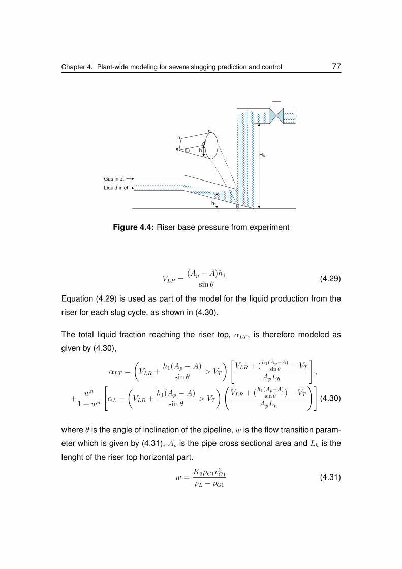
Chapter 4. Plant-wide modeling for severe slugging prediction and control 77
Figure 10 :Simplified Riser Model Showing Dynamical states
θ
θa
b
c
d
h1
h1
HR
Liquid inlet
Gas inlet
Figure 4.4: Riser base pressure from experiment
VLP =(Ap − A)h1
sin θ(4.29)
Equation (4.29) is used as part of the model for the liquid production from the
riser for each slug cycle, as shown in (4.30).
The total liquid fraction reaching the riser top, αLT , is therefore modeled as
given by (4.30),
αLT =
(VLR +
h1(Ap − A)
sin θ> VT
)[VLR + (h1(Ap−A)
sin θ− VT
ApLh
],
+wn
1 + wn
[αL −
(VLR +
h1(Ap − A)
sin θ> VT
)(VLR + (h1(Ap−A)
sin θ)− VT
ApLh
)](4.30)
where θ is the angle of inclination of the pipeline, w is the flow transition param-
eter which is given by (4.31), Ap is the pipe cross sectional area and Lh is the
lenght of the riser top horizontal part.
w =K3ρG1v
2G1
ρL − ρG1
(4.31)

78 Chapter 4. Plant-wide modeling for severe slugging prediction and control
4.3.4 Fluid flow out of the riser
Total fluid flow out of the riser, mmix, is calculated using a simplified valve equa-
tion given by (4.32), where K1 is the valve coefficient.
mmix = K1u
√ρT (PRT − Ps)
g(4.32)
The total fluid density, ρT , is given by (4.33), and gas density at riser top, ρG2,
is given by (4.34).
ρT = αLTρL + (1 + αLT )ρG2 (4.33)
The gas density at the riser top, ρG2, is given by (4.34) and the total volumetric
flow rate at the riser top is given by (4.35).
ρG2 =mG2
VG2
(4.34)
QT =mmix
ρT(4.35)
The gas mass flow rate out of the riser is given by (4.36), while the liquid mass
flow rate out of the riser is given by (4.37), where αmL is the liquid mass fraction.
mGout = (1− αmL )mmix (4.36)
mLout = αmLmmix (4.37)
4.3.4.1 Pressure driven fluid source
The modeling of the pressure driven source is considered very important due to
the dependency of the system stability and production on the pressure dynam-
ics of the entire system. The use of constant flow rate source in slug control
Chapter 4. Plant-wide modeling for severe slugging prediction and control 79
analysis does not represent the actual operating condition of the riser-pipeline
system in the offshore fields. Thus, the modeling of a pressure driven source
whose fluid supply is dependent on the pressure interaction with the down-
stream processes will be discussed in this section. These pressure interactions
and their effects on production will be discussed in detail in Chapter 6.
The pressure driven sources will differ in the environment of its application. In
the laboratory application, such as the Cranfield multiphase flow laboratory, the
pressure driven sources will be in the form of liquid pumps and gas compres-
sors. However, in the offshore oil and gas field, the pressure driven source
will be the oil and gas wells, and sometimes, a gas or liquid injection systems.
From these systems, the pressure driven source can be classified into two main
types, namely:
1. pressure driven liquid source
2. pressure driven gas source
In the offshore application, the pressure driven liquid source is the oil and water
wells, while in the laboratory application, it is the liquid pumps. The pressure
driven gas sources in the offshore application could be the gas wells and the
gas injection systems, while in the laboratory application, it is the gas compres-
sors. Among these systems, the focus will be on modeling the pressure driven
liquid sources. Since the pump delivery flow rate is controlled, the focus will be
on developing a linear liquid well model.
80 Chapter 4. Plant-wide modeling for severe slugging prediction and control
The linear well model as a pressure driven source
The linear well is modelled specifically to obtain the well liquid mass production
rate, qw. Detailed analysis of the properties of a linear well is given by Jamal et
al [49]. The linear well production rate is given by:
qw =Gf
Bµ(Pres − Pw) (4.38)
where B is the formation volume factor (FVF), µ is the viscosity of the liquid,
Pres is the reservoir pressure and Pw is the well bore hole pressure. Gf is the
reservoir geometric factor defined by:
Gf =2πBcKhhr
ln(ReqRw
) + s(4.39)
where Bc is the reservoir transmissibility factor, Kh is reservoir permeability,
Req is the reservoir external radius, Rw is the reservoir inner radius, hr is the
reservoir thickness and s is the reservoir skin (damage, 0 < s < 1).
The permeability, Kh is given by:
Kh = (KxKy)0.5 (4.40)
while the Req is given by:
Req = 0.28
[(KyKx
)0.5
L2x +
(KxKy
)0.5
L2y
]0.5
(KyKx
)0.25
+(KxKy
)0.25 (4.41)
where Kx is the reservoir permeability in the x-direction, Ky is the reservoir
permeability in the y-direction, Lx reservoir length in x-direction, Ly reservoir
length in y-direction.
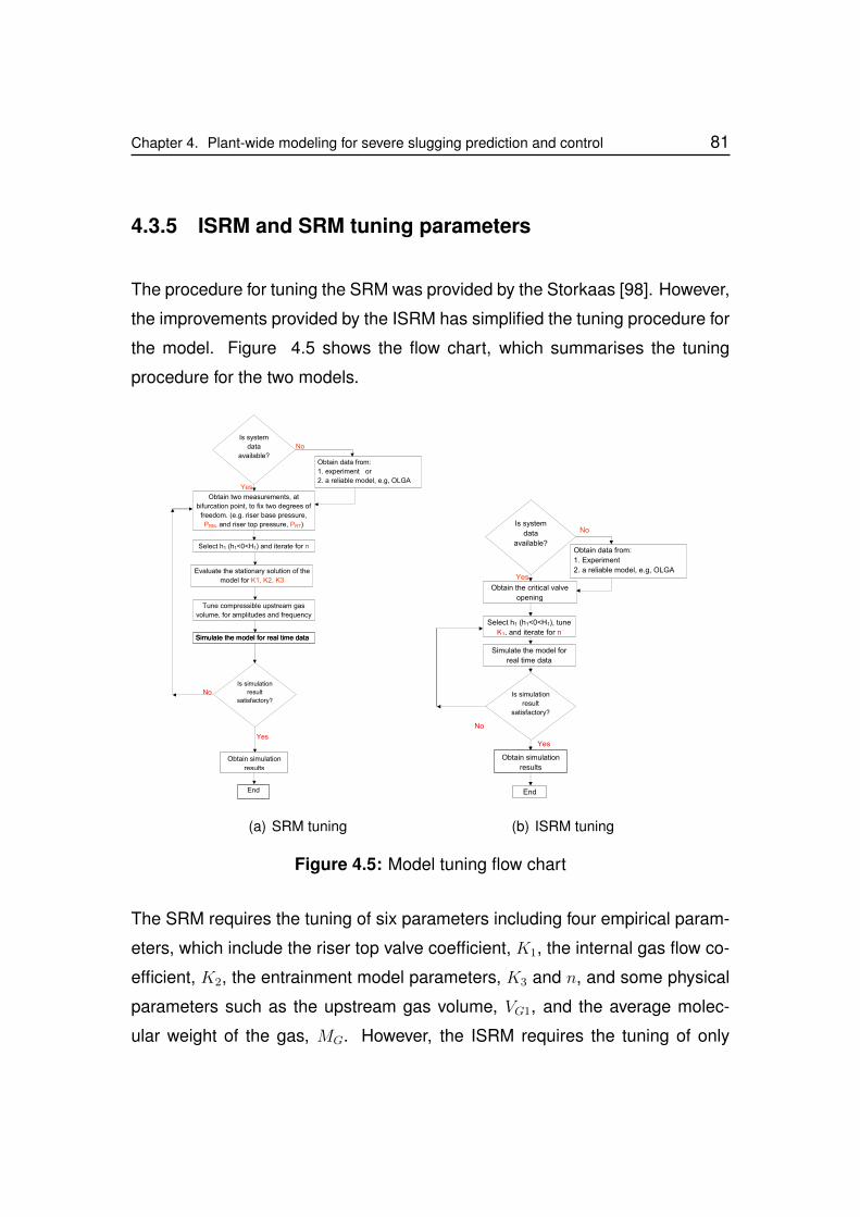
Chapter 4. Plant-wide modeling for severe slugging prediction and control 81
4.3.5 ISRM and SRM tuning parameters
The procedure for tuning the SRM was provided by the Storkaas [98]. However,
the improvements provided by the ISRM has simplified the tuning procedure for
the model. Figure 4.5 shows the flow chart, which summarises the tuning
procedure for the two models.
Is simulation
result
satisfactory?
Select h1 (h1<0<H1) and iterate for n
Evaluate the stationary solution of the
model for K1, K2, K3
Simulate the model for real time data
Is system
data
available?
Obtain two measurements, at
bifurcation point, to fix two degrees of
freedom. (e.g. riser base pressure,
PRB, and riser top pressure, PRT)
Yes
Tune compressible upstream gas
volume, for amplitudes and frequency
No
End
Obtain data from:
1. experiment or
2. a reliable model, e.g, OLGA
No
Simulate the model for real time data
Yes
Obtain simulation
results
(a) SRM tuning
Select h1 (h1<0<H1), tune
K1, and iterate for n
Simulate the model for
real time data
Is system
data
available?
Obtain the critical valve
opening
Yes
No
End
Obtain data from:
1. Experiment
2. a reliable model, e.g, OLGA
No
Is simulation
result
satisfactory?
Yes
Obtain simulation
results
(b) ISRM tuning
Figure 4.5: Model tuning flow chart
The SRM requires the tuning of six parameters including four empirical param-
eters, which include the riser top valve coefficient, K1, the internal gas flow co-
efficient, K2, the entrainment model parameters, K3 and n, and some physical
parameters such as the upstream gas volume, VG1, and the average molec-
ular weight of the gas, MG. However, the ISRM requires the tuning of only
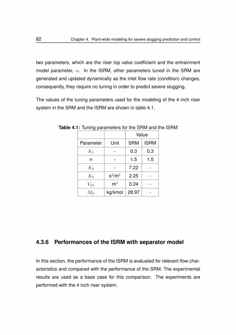
82 Chapter 4. Plant-wide modeling for severe slugging prediction and control
two parameters, which are the riser top valve coefficient and the entrainment
model parameter, n. In the ISRM, other parameters tuned in the SRM are
generated and updated dynamically as the inlet flow rate (condition) changes,
consequently, they require no tuning in order to predict severe slugging.
The values of the tuning parameters used for the modeling of the 4 inch riser
system in the SRM and the ISRM are shown in table 4.1.
Table 4.1: Tuning parameters for the SRM and the ISRMValue
Parameter Unit SRM ISRM
K1 - 0.3 0.3
n - 1.5 1.5
K2 - 7.22 -
K3 s2/m2 2.25 -
VG1 m3 0.24 -
MG kg/kmol 28.97 -
4.3.6 Performances of the ISRM with separator model
In this section, the performance of the ISRM is evaluated for relevant flow char-
acteristics and compared with the performance of the SRM. The experimental
results are used as a base case for this comparison. The experiments are
performed with the 4 inch riser system.
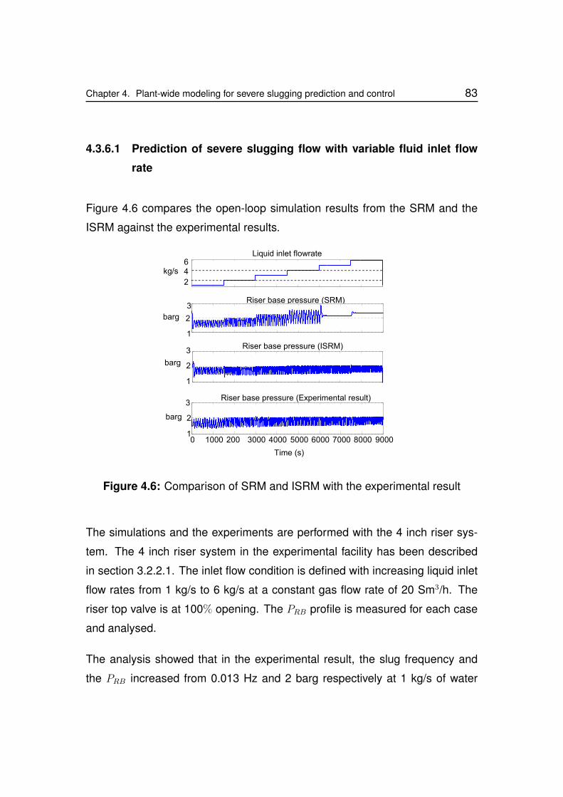
Chapter 4. Plant-wide modeling for severe slugging prediction and control 83
4.3.6.1 Prediction of severe slugging flow with variable fluid inlet flow
rate
Figure 4.6 compares the open-loop simulation results from the SRM and the
ISRM against the experimental results.
2
46
Liquid inlet flowrate
kg/s
0 1000 200 3000 4000 5000 6000 7000 8000 90001
2
3Riser base pressure (Experimental result)
barg
barg
Riser base pressure (SRM)3
2
1
1
2
3
barg
Riser base pressure (ISRM)
Time (s)
Figure 4.6: Comparison of SRM and ISRM with the experimental result
The simulations and the experiments are performed with the 4 inch riser sys-
tem. The 4 inch riser system in the experimental facility has been described
in section 3.2.2.1. The inlet flow condition is defined with increasing liquid inlet
flow rates from 1 kg/s to 6 kg/s at a constant gas flow rate of 20 Sm3/h. The
riser top valve is at 100% opening. The PRB profile is measured for each case
and analysed.
The analysis showed that in the experimental result, the slug frequency and
the PRB increased from 0.013 Hz and 2 barg respectively at 1 kg/s of water
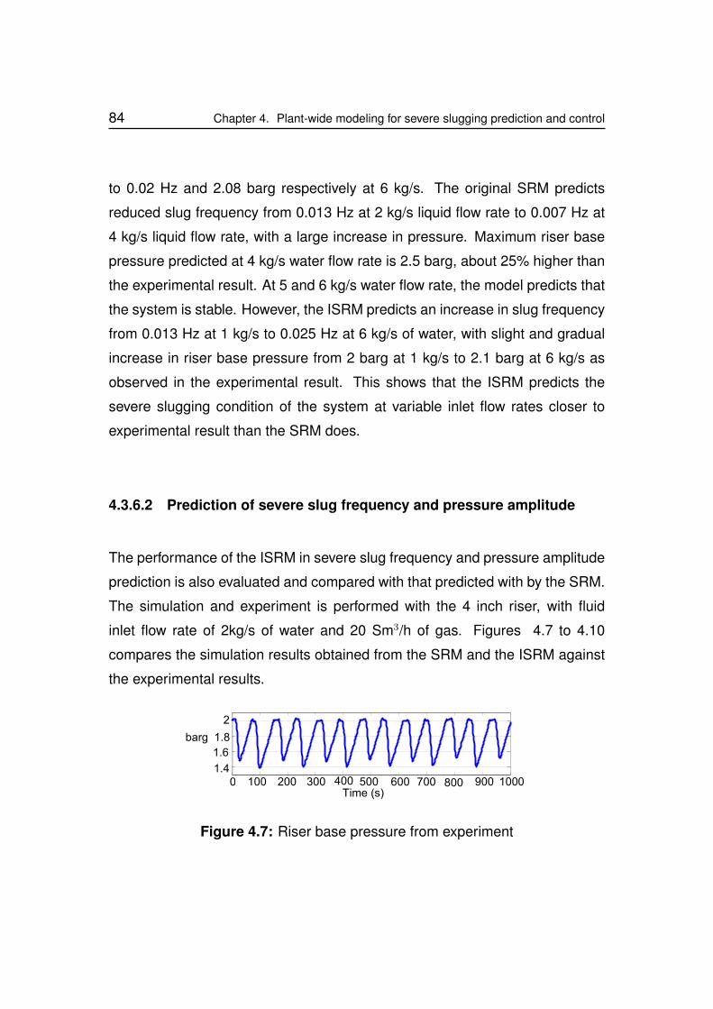
84 Chapter 4. Plant-wide modeling for severe slugging prediction and control
to 0.02 Hz and 2.08 barg respectively at 6 kg/s. The original SRM predicts
reduced slug frequency from 0.013 Hz at 2 kg/s liquid flow rate to 0.007 Hz at
4 kg/s liquid flow rate, with a large increase in pressure. Maximum riser base
pressure predicted at 4 kg/s water flow rate is 2.5 barg, about 25% higher than
the experimental result. At 5 and 6 kg/s water flow rate, the model predicts that
the system is stable. However, the ISRM predicts an increase in slug frequency
from 0.013 Hz at 1 kg/s to 0.025 Hz at 6 kg/s of water, with slight and gradual
increase in riser base pressure from 2 barg at 1 kg/s to 2.1 barg at 6 kg/s as
observed in the experimental result. This shows that the ISRM predicts the
severe slugging condition of the system at variable inlet flow rates closer to
experimental result than the SRM does.
4.3.6.2 Prediction of severe slug frequency and pressure amplitude
The performance of the ISRM in severe slug frequency and pressure amplitude
prediction is also evaluated and compared with that predicted with by the SRM.
The simulation and experiment is performed with the 4 inch riser, with fluid
inlet flow rate of 2kg/s of water and 20 Sm3/h of gas. Figures 4.7 to 4.10
compares the simulation results obtained from the SRM and the ISRM against
the experimental results.
1.4
1.6
1.8
2
barg
Time (s)0 100 200 300 400 500 600 700 800 900 1000
Figure 4.7: Riser base pressure from experiment
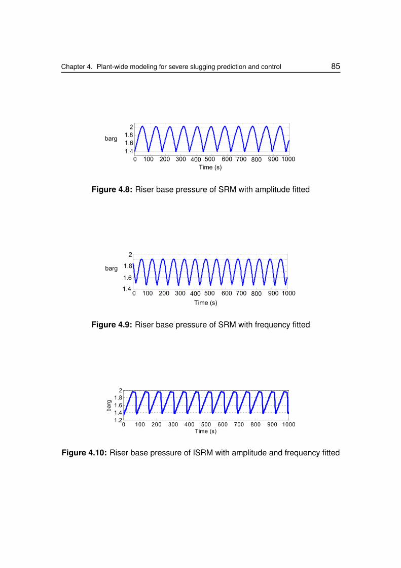
Chapter 4. Plant-wide modeling for severe slugging prediction and control 85
Time (s)
100 200 300 400 5001.4
1.6
1.8
2
barg
0 600 700 800 900 1000
Figure 4.8: Riser base pressure of SRM with amplitude fitted
1.4
1.6
1.8
2
barg
Time (s)
0 100 200 300 400 500 600 700 800 900 1000
Figure 4.9: Riser base pressure of SRM with frequency fitted
0 100 200 300 400 500 600 700 800 900 10001.2
1.4
1.6
1.8
2
Time (s)
ba
rg
Figure 4.10: Riser base pressure of ISRM with amplitude and frequency fitted
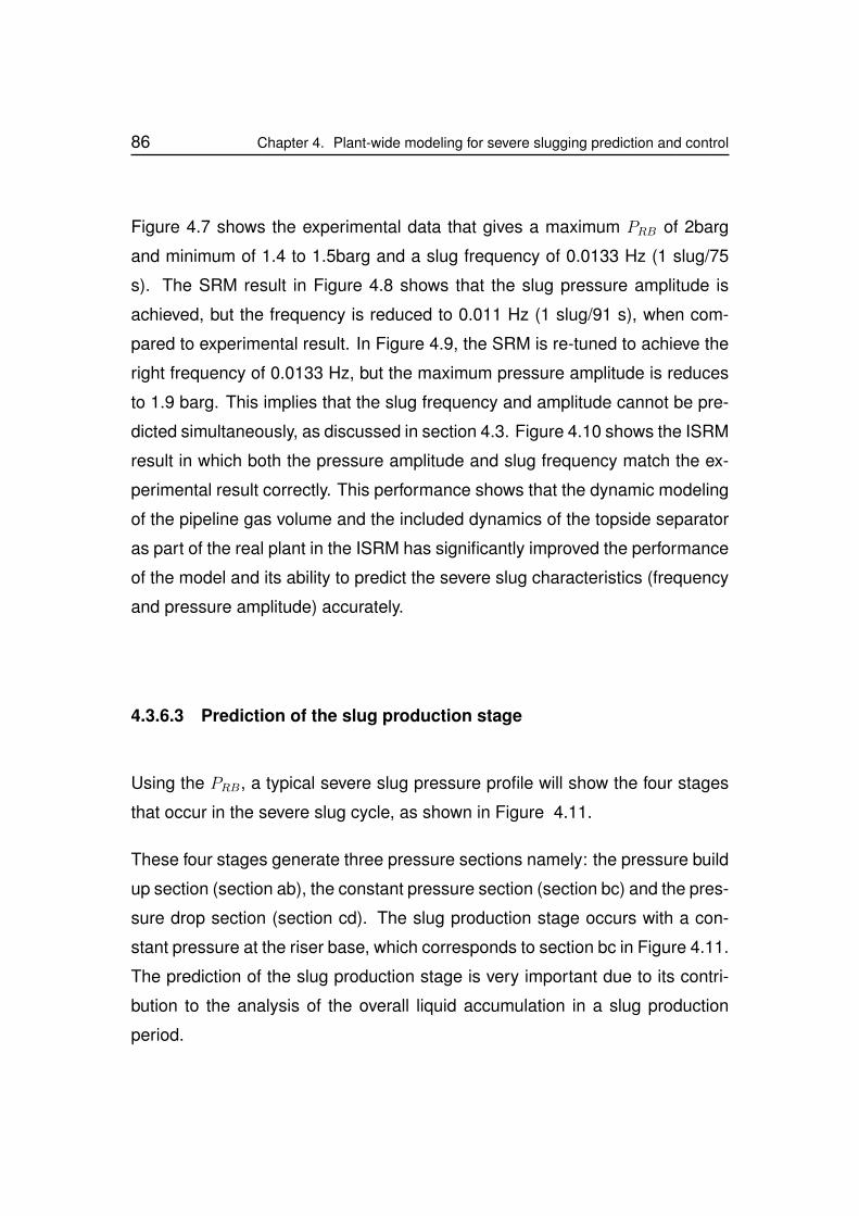
86 Chapter 4. Plant-wide modeling for severe slugging prediction and control
Figure 4.7 shows the experimental data that gives a maximum PRB of 2barg
and minimum of 1.4 to 1.5barg and a slug frequency of 0.0133 Hz (1 slug/75
s). The SRM result in Figure 4.8 shows that the slug pressure amplitude is
achieved, but the frequency is reduced to 0.011 Hz (1 slug/91 s), when com-
pared to experimental result. In Figure 4.9, the SRM is re-tuned to achieve the
right frequency of 0.0133 Hz, but the maximum pressure amplitude is reduces
to 1.9 barg. This implies that the slug frequency and amplitude cannot be pre-
dicted simultaneously, as discussed in section 4.3. Figure 4.10 shows the ISRM
result in which both the pressure amplitude and slug frequency match the ex-
perimental result correctly. This performance shows that the dynamic modeling
of the pipeline gas volume and the included dynamics of the topside separator
as part of the real plant in the ISRM has significantly improved the performance
of the model and its ability to predict the severe slug characteristics (frequency
and pressure amplitude) accurately.
4.3.6.3 Prediction of the slug production stage
Using the PRB, a typical severe slug pressure profile will show the four stages
that occur in the severe slug cycle, as shown in Figure 4.11.
These four stages generate three pressure sections namely: the pressure build
up section (section ab), the constant pressure section (section bc) and the pres-
sure drop section (section cd). The slug production stage occurs with a con-
stant pressure at the riser base, which corresponds to section bc in Figure 4.11.
The prediction of the slug production stage is very important due to its contri-
bution to the analysis of the overall liquid accumulation in a slug production
period.
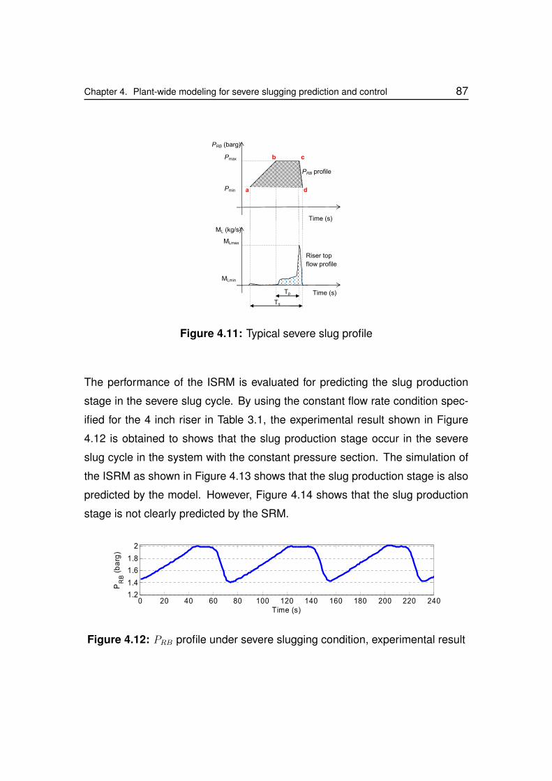
Chapter 4. Plant-wide modeling for severe slugging prediction and control 87
PRB (barg)
Pmax b c
PRB profile
Pmin a d
Time (s)
ML (kg/s)
MLmax
Riser top
flow profile
MLmin
Time (s)
Ts
Tp
Figure 4.11: Typical severe slug profile
The performance of the ISRM is evaluated for predicting the slug production
stage in the severe slug cycle. By using the constant flow rate condition spec-
ified for the 4 inch riser in Table 3.1, the experimental result shown in Figure
4.12 is obtained to shows that the slug production stage occur in the severe
slug cycle in the system with the constant pressure section. The simulation of
the ISRM as shown in Figure 4.13 shows that the slug production stage is also
predicted by the model. However, Figure 4.14 shows that the slug production
stage is not clearly predicted by the SRM.
0 20 40 60 80 100 120 140 160 180 200 220 2401.2
1.4
1.6
1.8
2
Time (s)
PR
B(b
arg
)
Figure 4.12: PRB profile under severe slugging condition, experimental result

88 Chapter 4. Plant-wide modeling for severe slugging prediction and control
0 20 40 60 80 100 120 140 160 180 200 220 2401.2
1.4
1.6
1.8
2
Time (s)
PR
B(b
arg
)
Figure 4.13: PRB profile under severe slugging condition, ISRM
0 20 40 60 80 100 120 140 160 180 200 220 2401.2
1.4
1.6
1.8
2
Time (s)
PR
B(b
arg
)
Figure 4.14: PRB profile under severe slugging condition, SRM
This result shows the close agreement between the ISRM results and the ex-
perimental results. This makes the ISRM a more reliable model for severe slug
characteristic prediction and control performance analysis.
4.3.6.4 Prediction of flow regime map
The performance of the ISRM shows that it can be used to predict severe slug
flow regime for a riser-pipeline production system. Various flow combinations
can be simulated continuously to predict the flow condition with relative accu-
racy when compared to experimental result. The prediction of severe slug flow
regime map for the 4 inch riser at the multiphase flow laboratory of Cranfield
University is carried out through experimental study and the ISRM simulation.
About 194 test points for different liquid and gas combinations were simulated.
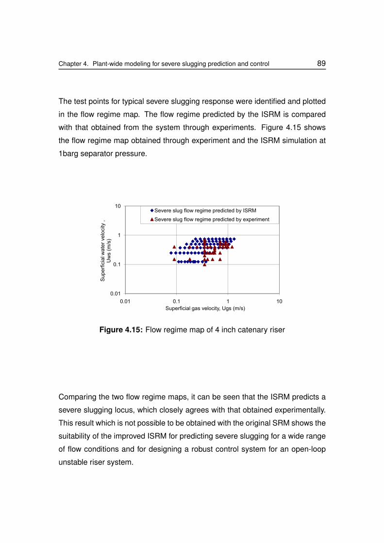
Chapter 4. Plant-wide modeling for severe slugging prediction and control 89
The test points for typical severe slugging response were identified and plotted
in the flow regime map. The flow regime predicted by the ISRM is compared
with that obtained from the system through experiments. Figure 4.15 shows
the flow regime map obtained through experiment and the ISRM simulation at
1barg separator pressure.
0.01
0.1
1
10
0.01 0.1 1 10
Su
pe
rfic
ialw
ate
rve
loci
ty,
Uw
s(m
/s)
Superficial gas velocity, Ugs (m/s)
Severe slug flow regime predicted by ISRM
Severe slug flow regime predicted by experiment
Figure 4.15: Flow regime map of 4 inch catenary riser
Comparing the two flow regime maps, it can be seen that the ISRM predicts a
severe slugging locus, which closely agrees with that obtained experimentally.
This result which is not possible to be obtained with the original SRM shows the
suitability of the improved ISRM for predicting severe slugging for a wide range
of flow conditions and for designing a robust control system for an open-loop
unstable riser system.
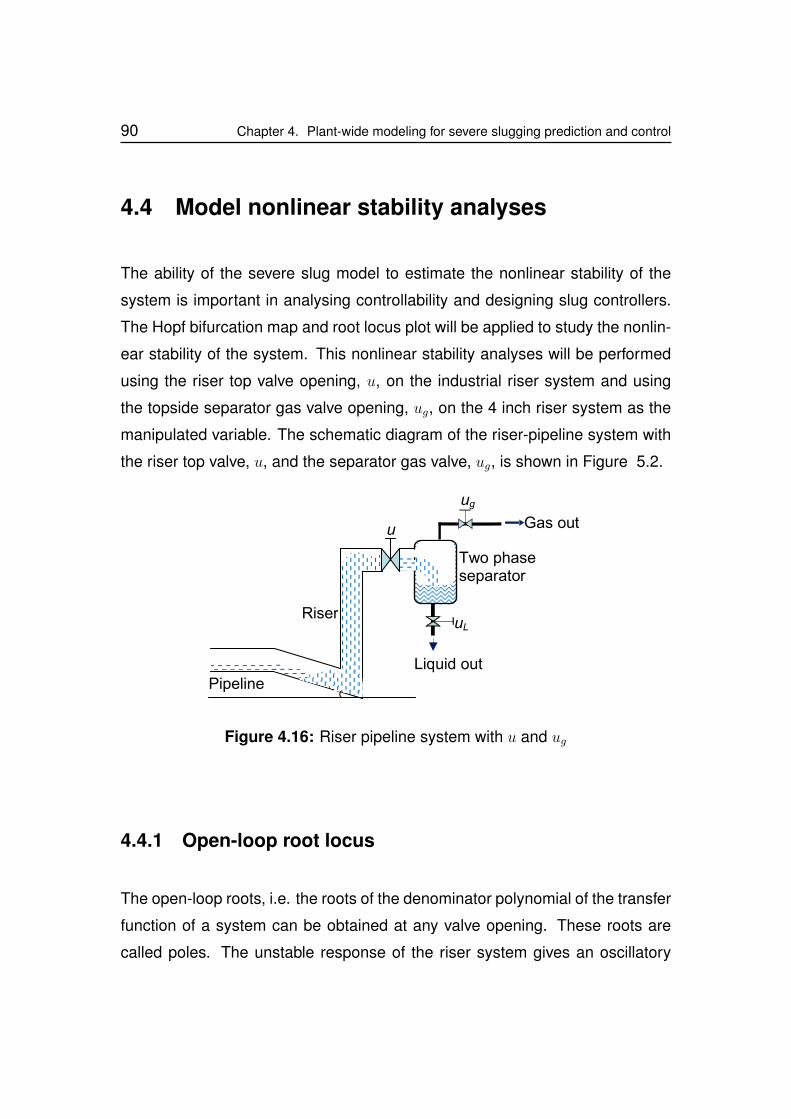
90 Chapter 4. Plant-wide modeling for severe slugging prediction and control
4.4 Model nonlinear stability analyses
The ability of the severe slug model to estimate the nonlinear stability of the
system is important in analysing controllability and designing slug controllers.
The Hopf bifurcation map and root locus plot will be applied to study the nonlin-
ear stability of the system. This nonlinear stability analyses will be performed
using the riser top valve opening, u, on the industrial riser system and using
the topside separator gas valve opening, ug, on the 4 inch riser system as the
manipulated variable. The schematic diagram of the riser-pipeline system with
the riser top valve, u, and the separator gas valve, ug, is shown in Figure 5.2.
Two phaseseparator
Liquid out
Gas out
uLRiser
Pipeline
ug
u
Figure 4.16: Riser pipeline system with u and ug
4.4.1 Open-loop root locus
The open-loop roots, i.e. the roots of the denominator polynomial of the transfer
function of a system can be obtained at any valve opening. These roots are
called poles. The unstable response of the riser system gives an oscillatory
Chapter 4. Plant-wide modeling for severe slugging prediction and control 91
response corresponding to a pair of complex poles, x + iy, with x > 0. Poles
can be plotted in the complex plane (s-plane), which has real axis (horizontal-
axis) and imaginary axis (vertical-axis). The location of pole(s) obtained at a
particular valve opening on the s-plane gives a clear indication on the stability
of the plant at that operating point. A pair of complex poles with positive real
parts indicates system instability and is located in the right half plane (RHP)
of the s-plane. However, for a stable system, all the poles must be located in
the left half plane (LHP). This implies that all the poles of a stable system must
have a negative real part. Further explanations on why the presence of RHP
poles will cause system instability can be found in literature [92, 94].
4.4.2 Hopf bifurcation map
The Hopf bifurcation is a type of bifurcation which occurs when a pair of com-
plex poles crosses the imaginary axis from the left hand plane (LHP) to the right
half plane (RHP) of the s-plane. Such crossing of a pair of complex poles across
the imaginary axis of the s-plane leads to the vanishing of linear damping in the
motion of an oscillator [111]. Thus, when Hopf bifurcation occurs in a system,
there is a loss of stability in the system’s controlled variable due to changes in
an independent variable. For a nonlinear system like the riser-pipeline system,
Hopf bifurcation can occur in the controlled variable if changes in an indepen-
dent variable such as the valve opening causes the system to become unstable
at any operating point. The Hopf bifurcation map of a riser-pipeline system can
be generated through experimental and simulation studies. The ability of the
ISRM to generate the bifurcation map is very important in the analysis of control
performance of the riser-pipeline system.
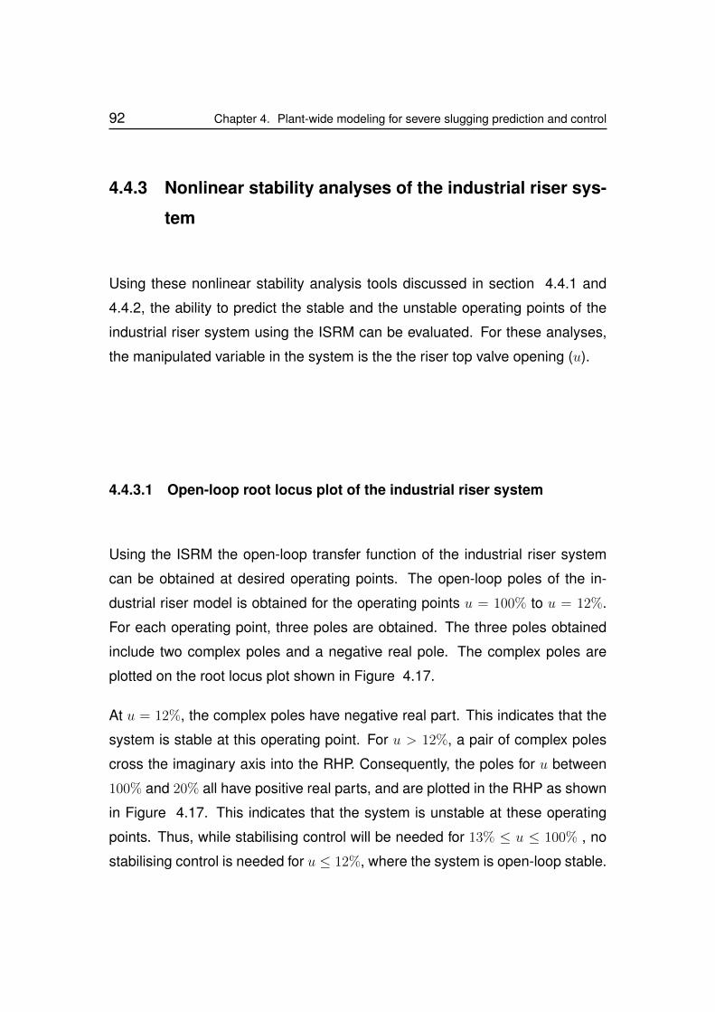
92 Chapter 4. Plant-wide modeling for severe slugging prediction and control
4.4.3 Nonlinear stability analyses of the industrial riser sys-
tem
Using these nonlinear stability analysis tools discussed in section 4.4.1 and
4.4.2, the ability to predict the stable and the unstable operating points of the
industrial riser system using the ISRM can be evaluated. For these analyses,
the manipulated variable in the system is the the riser top valve opening (u).
4.4.3.1 Open-loop root locus plot of the industrial riser system
Using the ISRM the open-loop transfer function of the industrial riser system
can be obtained at desired operating points. The open-loop poles of the in-
dustrial riser model is obtained for the operating points u = 100% to u = 12%.
For each operating point, three poles are obtained. The three poles obtained
include two complex poles and a negative real pole. The complex poles are
plotted on the root locus plot shown in Figure 4.17.
At u = 12%, the complex poles have negative real part. This indicates that the
system is stable at this operating point. For u > 12%, a pair of complex poles
cross the imaginary axis into the RHP. Consequently, the poles for u between
100% and 20% all have positive real parts, and are plotted in the RHP as shown
in Figure 4.17. This indicates that the system is unstable at these operating
points. Thus, while stabilising control will be needed for 13% ≤ u ≤ 100% , no
stabilising control is needed for u ≤ 12%, where the system is open-loop stable.
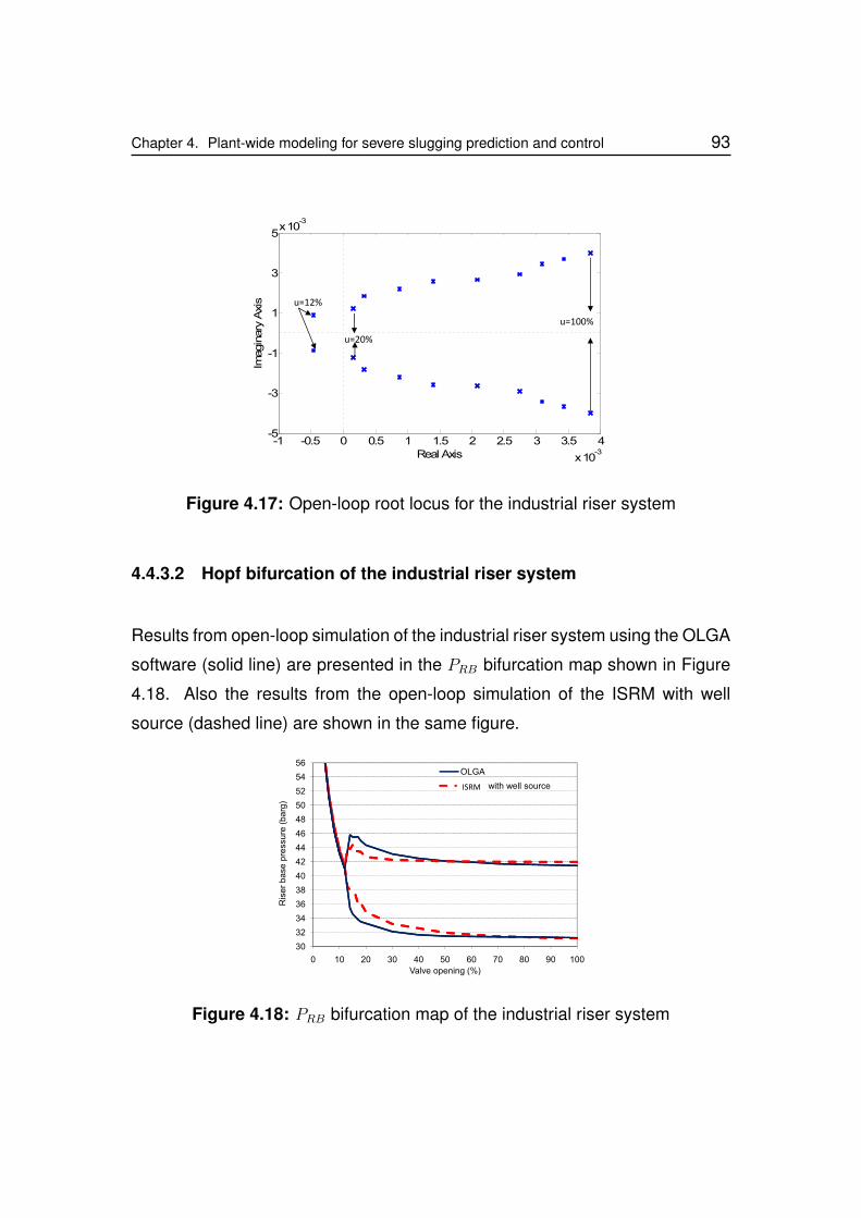
Chapter 4. Plant-wide modeling for severe slugging prediction and control 93
-1 -0.5 0 0.5 1 1.5 2 2.5 3 3.5 4
x10-3
-5
-3
-1
1
3
5x10
-3
Real Axis
Imagin
ary
Axis
u=20%
u=12%
u=100%
Figure 4.17: Open-loop root locus for the industrial riser system
4.4.3.2 Hopf bifurcation of the industrial riser system
Results from open-loop simulation of the industrial riser system using the OLGA
software (solid line) are presented in the PRB bifurcation map shown in Figure
4.18. Also the results from the open-loop simulation of the ISRM with well
source (dashed line) are shown in the same figure.
30
32
34
36
38
40
42
44
46
48
50
52
54
56
0 10 20 30 40 50 60 70 80 90 100
Ris
er
ba
sep
ress
ure
(ba
rg)
Valve opening (%)
OLGA
SRSM with well sourceISRM
Figure 4.18: PRB bifurcation map of the industrial riser system
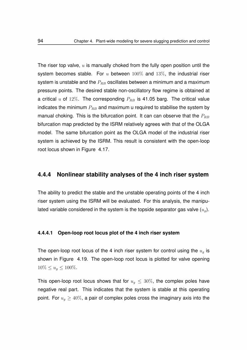
94 Chapter 4. Plant-wide modeling for severe slugging prediction and control
The riser top valve, u is manually choked from the fully open position until the
system becomes stable. For u between 100% and 13%, the industrial riser
system is unstable and the PRB oscillates between a minimum and a maximum
pressure points. The desired stable non-oscillatory flow regime is obtained at
a critical u of 12%. The corresponding PRB is 41.05 barg. The critical value
indicates the minimum PRB and maximum u required to stabilise the system by
manual choking. This is the bifurcation point. It can can observe that the PRB
bifurcation map predicted by the ISRM relatively agrees with that of the OLGA
model. The same bifurcation point as the OLGA model of the industrial riser
system is achieved by the ISRM. This result is consistent with the open-loop
root locus shown in Figure 4.17.
4.4.4 Nonlinear stability analyses of the 4 inch riser system
The ability to predict the stable and the unstable operating points of the 4 inch
riser system using the ISRM will be evaluated. For this analysis, the manipu-
lated variable considered in the system is the topside separator gas valve (ug).
4.4.4.1 Open-loop root locus plot of the 4 inch riser system
The open-loop root locus of the 4 inch riser system for control using the ug is
shown in Figure 4.19. The open-loop root locus is plotted for valve opening
10% ≤ ug ≤ 100%.
This open-loop root locus shows that for ug ≤ 30%, the complex poles have
negative real part. This indicates that the system is stable at this operating
point. For ug ≥ 40%, a pair of complex poles cross the imaginary axis into the

Chapter 4. Plant-wide modeling for severe slugging prediction and control 95
-0.4 -0.3 -0.2 -0.1 0 0.1 0.2-0.2
-0.15
-0.1
-0.05
0
0.05
0.1
0.15
0.2
Real Axis
Ima
gin
ary
Axis
ug=100%ug=30%
Figure 4.19: Open-loop root locus for the 4 inch riser system
RHP. Consequently, the poles for ug between 100% and 40% all have positive
real parts, and are plotted in the RHP as shown in Figure 4.19. This indicates
that the system is unstable at these operating points. Thus, while stabilising
control will be needed for 40% ≤ ug ≤ 100% , no stabilising control is needed
for ug ≤ 30%, where the system is open-loop stable.
4.4.4.2 Hopf Bifurcation of the 4 inch riser system
The Hopf bifurcation map of the 4 inch riser system for open-loop control using
the ug, on the ISRM and on the experimental facility is also evaluated. Figure
4.20 shows the PRB Hopf bifurcation map obtained through open-loop simu-
lation of the 4 inch riser system using the ISRM (solid line) and that obtained
through experiment on the same system (dashed line).
The experimental results show that the system is unstable and the PRB oscil-
lates between minimum and maximum pressure points for ug ≥ 40%. Also, the
96 Chapter 4. Plant-wide modeling for severe slugging prediction and control
1.4
1.5
1.6
1.7
1.8
1.9
2
2.1
2.2
2.3
2.4
0 10 20 30 40 50 60 70 80 90 100
Ris
er
ba
sep
ress
ure
(ba
rg)
Valve opening (%)
Experiment
SRSMISRM
Figure 4.20: Pressure bifurcation map of the 4 inch riser system
Hopf bifurcation point occur at a critical valve opening of ug = 40%, such that
the desired stable non-oscillatory flow regime is obtained. It can be observe
that the bifurcation map predicted by the ISRM closely agree with the experi-
mental result. The corresponding PRB from the ISRM and from the experiment
are 1.97 barg and 1.95 barg respectively. This result is consistent with the
open-loop root locus presented in section 4.4.4.1.
These results show the ability of the ISRM to accurately predict relevant control
properties required for slug controller design, for different control structures and
riser-pipeline geometry.
4.5 Conclusions
In this chapter, the development of the plant-wide model for severe slug con-
trol is presented. The modeling of the riser slugging using a plant-wide model,
which requires the modeling of the riser-pipeline system and its integration with
the model of the two phase separator system and the pressure dependent well
Chapter 4. Plant-wide modeling for severe slugging prediction and control 97
model is achieved. Through the development of the plant-wide model, the ISRM
is developed to eliminate some assumptions and limitations of the SRM in pre-
dicting severe slugging.
Simulation results from the SRM and the ISRM shows that the ISRM predicts
severe slug characteristics, such as pressure amplitude and slug frequency
more closely to the experimental result than the SRM. Also, the ability to pre-
dict severe slugging characteristics with changing inlet flow condition, which is
not possible with the SRM is achieved with the ISRM. Improved performance is
achieved with the ISRM in the prediction of the slug production stage in the se-
vere slug cycle, when compared to the SRM, against the experimental results.
The ability of the ISRM to predict relevant nonlinear stability is investigated
using the industrial riser system and a 4 inch laboratory riser system. Its pre-
diction of these nonlinear stabilities showed close agreement with experimental
results.

98 Chapter 4. Plant-wide modeling for severe slugging prediction and control
Chapter 5
Controllability analysis of unstable
riser-pipeline system
5.1 Introduction
In this chapter, the controllability analysis of an unstable riser-pipeline system
is presented. The focus of the controllability analysis in this work is on the
input-output controllability concept. Thus, the aim of the controllability analy-
sis is to verify to what extent the system can achieve the desired performance
objectives. In the input-output controllability analysis concept, a system is de-
scribed as controllable if there exists a controller that can stabilise the system
and provide acceptable system performance(s) [94]. As was pointed out by
Skogestad and Postlethwaite, [94], input-output controllability differs from the
state controllability analysis, which was introduced by Kalman [54, 55]. In the
state controllability theory, a system is considered to be controllable if every
desired transition of the plants state from a given initial state to any final state
can be effected in a finite time by some unconstrained control inputs [54, 55].
In view of this, state controllability analysis does not consider the quality of the
99
100 Chapter 5. Controllability analysis of unstable riser-pipeline system
response between the two states, and the input magnitude required could be
large. Thus, in this work, the focus is on the input-output controllability con-
cept. The input-output controllability will simply be called controllability, since it
is clear that the state controllability is not considered.
The controllability of a system will depend on a number of system related fac-
tors, including the choice of control structure, the operating condition(s) and the
system (riser-pipeline) design. A system’s controllability analysis can be per-
formed with focus on all or one of these factors. In each case, certain (relevant)
control objectives are imposed on the system and the ability of the system to
achieve them is analysed using relevant control theories.
In the controllability analysis of the riser-pipeline-system presented in this work,
the control objectives are focused on the core operational targets and the direct
benefits that are required from the control of an unstable riser-pipeline system.
These direct benefits include, the ability to stablise the system as well as max-
imise (increase) oil production. The interdependency between a stable valve
opening and the accumulated production is explored as the fundamental basis
for the controllability analysis. The system related factors such as the choice of
control structure and the operating conditions which affect the system’s ability
to achieve these control objectives are considered in the course of this control-
lability analysis.
Control strategies which are considered particularly relevant to the riser-pipeline
system are considered. The system’s nonlinearity, which affects its character-
istics and ability to achieve stability at any desired valve opening is considered.
Relevant control theories which provide key insights in the closed-loop control
performance of a system are applied in the analysis of the control performance
of the nonlinear model in a feedback loop.
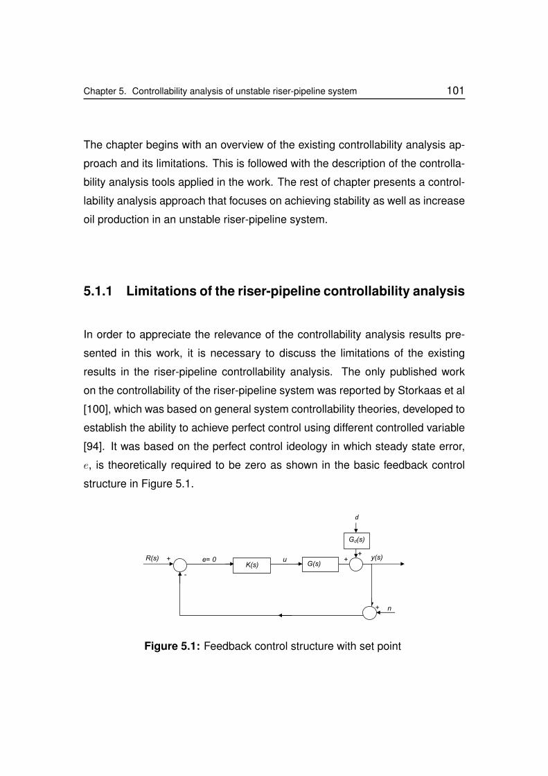
Chapter 5. Controllability analysis of unstable riser-pipeline system 101
The chapter begins with an overview of the existing controllability analysis ap-
proach and its limitations. This is followed with the description of the controlla-
bility analysis tools applied in the work. The rest of chapter presents a control-
lability analysis approach that focuses on achieving stability as well as increase
oil production in an unstable riser-pipeline system.
5.1.1 Limitations of the riser-pipeline controllability analysis
In order to appreciate the relevance of the controllability analysis results pre-
sented in this work, it is necessary to discuss the limitations of the existing
results in the riser-pipeline controllability analysis. The only published work
on the controllability of the riser-pipeline system was reported by Storkaas et al
[100], which was based on general system controllability theories, developed to
establish the ability to achieve perfect control using different controlled variable
[94]. It was based on the perfect control ideology in which steady state error,
e, is theoretically required to be zero as shown in the basic feedback control
structure in Figure 5.1.
e= 0G(s)K(s)
+
-
u y(s)R(s)
Gd(s)
d
n
++
+
Figure 5.1: Feedback control structure with set point
102 Chapter 5. Controllability analysis of unstable riser-pipeline system
Based on the concept of perfect control, certain control objectives were im-
posed on the riser system. These control objectives include:
1. perfect disturbance rejection (disturbances due to the topside separator
pressure and the liquid and gas flow rate)
2. perfect tracking of controlled variable set point
3. suppressing measurement noise
Some conclusions based on their controllability analysis pointed out that certain
controlled variables such as the riser top pressure, PRT , will not be suitable for
slug control of the unstable riser-pipeline system, while the riser base pressure
PRB will be the most suitable controlled variable.
In view of the desired performance required from the control of unstable riser-
pipeline system, it is clear that these control objectives does not reflect the real
needs required by a practical slug control system. Practically, the controllability
analysis of the unstable riser-pipeline should indicate the extent to which the
control system is able to stablise the unstable riser-pipeline with maximised
production. Thus, it is important to consider a more appropriate control strategy
to analyse the controllability of the unstable riser-pipeline system. This will
require:
1. defining the control objectives of the system that are relevant to the oil
and gas production
2. implementing an appropriate control strategy which can achieve the con-
trol objectives
Chapter 5. Controllability analysis of unstable riser-pipeline system 103
By adopting more appropriate control objectives, the analyses of the ability
to stabilise the unstable riser-pipeline system and maximise production, using
various controlled variables, including the PRT which had been considered un-
suitable for slug control of the unstable riser-pipeline system will be carried out.
5.2 Controllability analysis tools
The focus of the controllability analysis presented in this work is on the ability
to achieve closed-loop stability with maximised oil production. The analysis
of these controllability issues requires using relevant control theories. Firstly,
the description of the control objectives that are relevant to the riser-pipeline
system is presented.
5.2.1 Control objectives
A suitable approach in the controllability analysis of the riser-pipeline system is
to define the control objectives to reflect and address the core operation targets
of an unstable riser-pipeline system. These will be system specific and differ
from the general control objectives mentioned earlier in section 5.1.1. From
the riser-pipeline production system point of view, the slug control objectives
should focus on:
1. achieving stable operation
2. maximising (increasing) production
104 Chapter 5. Controllability analysis of unstable riser-pipeline system
In view of these objectives, the perfect control of the controlled variable set point
in riser pipeline system will not be necessary, as it does not provide any benefit
to the oil production system operation. The relevant basic control structure
which is practically relevant for achieving these objectives will be discussed and
implemented in section 5.5.2. Next, the relationship between valve opening
and production will be briefly discussed.
5.2.2 Valve opening and production
The ability to maximise production using the result based on the stability per-
formance of the system is analysed. Depending on the control structure, a
number of controlled variables including the riser base pressure (PRB), riser
top pressure (PRT ), total volumetric flowrate at the riser outlet (QT ) and the
topside separator pressure (Ps), could be used for the unstable riser-pipeline
system control. Whichever controlled variable is used, the fundamental ob-
jective should be the ability to stabilise the system at a valve opening that is
large enough to ensure maximum production. The analysis of production de-
pendency on the flow line pressure is discussed in Chapter 6, where it will be
shown that, an increase in the production rate can be achieved by reducing
PRB, which depends on a number of system related factors including the pres-
sure loss across the valve, (DPu).
Assuming a linear valve characteristics, the relationship between the DPu and
the valve opening, u, can approximately be defined as:
DPu ∝1
u2(5.1)
Equation 5.1 shows that relatively small valve opening will result in high DPu
and consequently high PRB. Conversely, relatively large valve opening will re-
Chapter 5. Controllability analysis of unstable riser-pipeline system 105
sult in low DPu and consequently low PRB. Thus, in order to reduce the PRB,
we are required to achieve system stability at a relatively large valve opening.
5.2.3 Lower bound on the input magnitude
The analysis of the lower bound on the input usage will be employed to eval-
uate the ability of the control system to achieve closed-loop stability at large
valve opening as required in the control objectives discussed in section 5.2.1.
The unstable riser system cannot be stabilised at any open-loop operating point
if the control input saturates, such that the scaled control input magnitude re-
quired to stabilise the system at that operating point is greater than or equal to
1 (|u| ≥ 1). Thus, the analysis of the input magnitude, |u|, which is required to
stabilise the system at any open-loop unstable valve opening is very important.
The previous work by Glover [31] showed that the input magnitude required to
stabilise the system at each open-loop unstable valve opening can be obtained
by evaluating lower bound onKS, which is defined as a function of the minimum
Hankel Singular Value of the plant, as given in (5.2), (see also Skogestaad and
Postlethwaite [94]).
‖KS‖∞ ≥1
σ¯H
(U(G))(5.2)
where U(G) is the unstable part of G, K is the controller and S is the sensitivity
function defined as S = (1 +GK)−1.
Equation 5.2 gives the lower bound of the input magnitude which is required to
stabilise the system. This implies that by evaluating the right-hand-side (RHS)
of (5.2), the minimum input magnitude required to stabilise the system will be
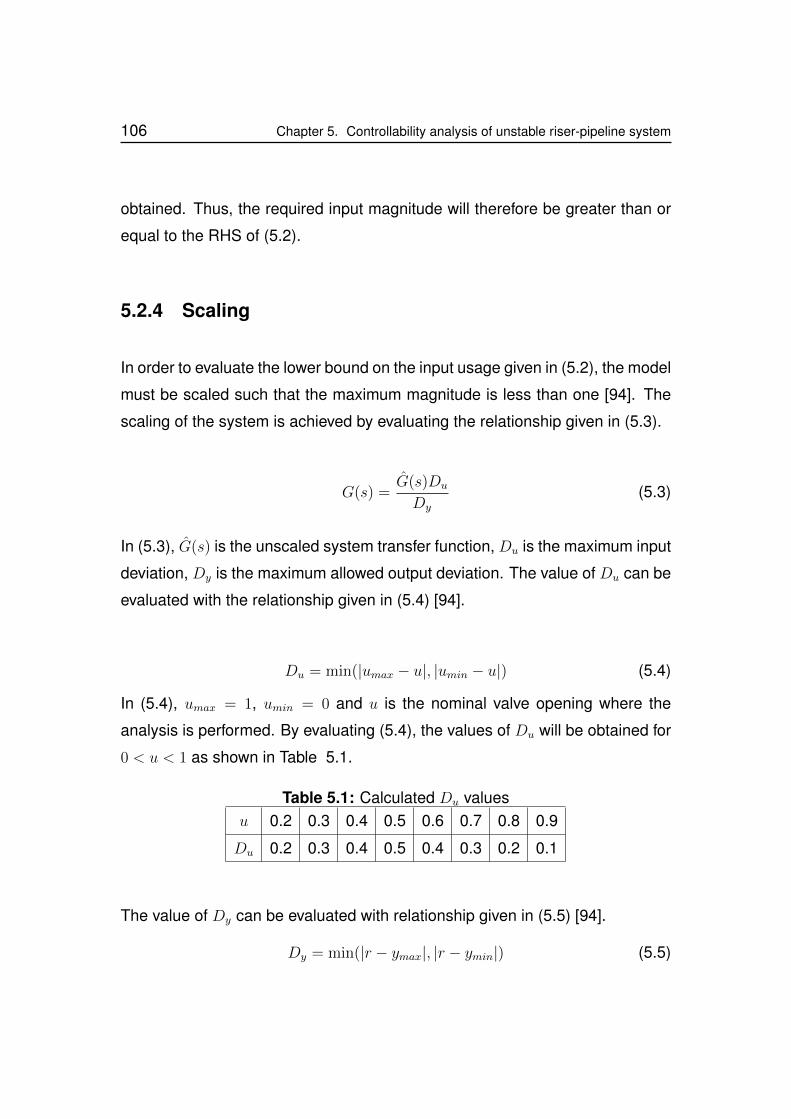
106 Chapter 5. Controllability analysis of unstable riser-pipeline system
obtained. Thus, the required input magnitude will therefore be greater than or
equal to the RHS of (5.2).
5.2.4 Scaling
In order to evaluate the lower bound on the input usage given in (5.2), the model
must be scaled such that the maximum magnitude is less than one [94]. The
scaling of the system is achieved by evaluating the relationship given in (5.3).
G(s) =G(s)Du
Dy
(5.3)
In (5.3), G(s) is the unscaled system transfer function, Du is the maximum input
deviation, Dy is the maximum allowed output deviation. The value of Du can be
evaluated with the relationship given in (5.4) [94].
Du = min(|umax − u|, |umin − u|) (5.4)
In (5.4), umax = 1, umin = 0 and u is the nominal valve opening where the
analysis is performed. By evaluating (5.4), the values of Du will be obtained for
0 < u < 1 as shown in Table 5.1.
Table 5.1: Calculated Du valuesu 0.2 0.3 0.4 0.5 0.6 0.7 0.8 0.9
Du 0.2 0.3 0.4 0.5 0.4 0.3 0.2 0.1
The value of Dy can be evaluated with relationship given in (5.5) [94].
Dy = min(|r − ymax|, |r − ymin|) (5.5)
Chapter 5. Controllability analysis of unstable riser-pipeline system 107
In (5.5), ymax and ymin are the maximum and minimum values of the controlled
variable at each operating point defined by the valve opening respectively. Also,
r is the set point of the controlled variable, which is desired at steady state. For
an open-loop unstable operating point, the value of r will be equal to the value
of the controlled variable at the corresponding unstable equilibrium point. Thus,
the Dy can be calculated by evaluating the maximum allowed deviation from the
value of the controlled variable at the unstable equilibrium point at each valve
opening. This analysis can easily be performed using the Hopf bifurcation map
of the controlled variable. This will be explained in details in section 5.3.1.
The first step to performing these controllability analyses is to obtain the linear
model transfer function of the system at the open-loop unstable valve openings.
These linear model transfer functions can be defined in a general form as a
function of the unstable steady state valve opening for each controlled variable.
5.2.5 Linear model transfer functions
Consider a hypothetical three state unstable system with the linear model trans-
fer function as given in (5.6).
G(s) =b0
s3 + a2s2 − a1s+ a0
(5.6)
The value of the coefficients a2, a1, a0 and b0 will depend on the steady state
valve opening (ue) in which the linear model is obtained. For a set of steady
state valve openings (uei), a set of linear system models, Gi(s, ue), will be ob-
tained for each ue, for i = 1, 2, ..., n, where n is the number of linear model
transfer functions obtained from the system. If the coefficients a2, a1, a0 and b0
108 Chapter 5. Controllability analysis of unstable riser-pipeline system
in (5.6) are defined as nonlinear functions as given in (5.7), the general form of
the linear model, G(s, ue), can be defined as given in (5.8). Thus, for a given
ue, the corresponding linear model of the system is obtained by evaluating the
nonlinear functions in (5.7) and substituting in (5.8).
a2 = f2(ue), a1 = f1(ue), a0 = f0(ue), b0 = g0(ue) (5.7)
Gi(s, ue) =g0(ue)
s3 + f2(ue)s2 − f1(ue)s+ f0(ue)(5.8)
The linear model transfer function of the riser-pipeline system can be defined in
this general form, with the numerator and the denominator coefficients defined
by nonlinear functions. The system’s linear model transfer function can then be
obtained at any desired steady state valve opening in the open-loop unstable
region, if the relationship for the nonlinear functions are defined as a function
of the steady state valve opening. Next, the methods which can be applied to
derive these nonlinear functions will be discussed.
5.2.5.1 Deriving the nonlinear functions
Consider a nonlinear system represented by a general state space form given
by (5.9) and (5.10)
x = f(x, u) (5.9)
y = g(x, u) (5.10)
Chapter 5. Controllability analysis of unstable riser-pipeline system 109
where x is the state variable, y is the output and u is the input variable (valve
opening). A linear model of (5.9) and (5.10) can be obtained at an unstable
steady state operating point defined by, (xe, ue), such that:
0 = f(xe, ue) (5.11)
ye = g(xe, ue) (5.12)
and the obtained linear model in terms of the deviation terms is given as:
δx = Aδx+Bδu (5.13)
δy = Cδx+Dδu (5.14)
In (5.13) and (5.14), δx can be replaced by x, and δu can be replaced by u.
Also in (5.14), δy can also be replaced by y, such that x, y and u denotes the
deviation from the equilibrium. Thus, (5.13) and (5.14) can be simplified as
given in (5.15) and (5.16) respectively,
x = Ax+Bu (5.15)
y = Cx+Du (5.16)
where A is the state matrix, B is the input matrix, C is the output matrix and D
is the input-output direct coupling matrix. The matrices of the linearised model
are obtained as partial derivatives of the dynamical state equations and are
given as:
A =
∣∣∣∣∂f∂x∣∣∣∣xe,ue
, B =
∣∣∣∣∂f∂u∣∣∣∣xe,ue
, C =
∣∣∣∣∂g∂x∣∣∣∣xe,ue
, D =
∣∣∣∣∂g∂u∣∣∣∣xe,ue
(5.17)
110 Chapter 5. Controllability analysis of unstable riser-pipeline system
From (5.17), the linear system transfer function from the input, u, to the output,
y, can be obtained as:
y(s)
u(s)= C(Is− A)−1B +D (5.18)
In order to determine the linear model transfer function as given in (5.18), the
state matrix (A), the input matrix (B), the output matrix (C) and the input-output
direct coupling matrix (D), could be defined as a function of the physical sys-
tem variables. However, for high order and multi-variable systems, this method
can become complicated. A less complicated method is a numerical solution
which can be achieved by determining a nonlinear empirical function that ap-
proximates the value of the coefficients in the linear model. To achieve this,
a basic knowledge of the system’s transfer functions is required. This can be
obtained by using any suitable system identification method. However, for a
system whose mechanistic model has been developed, such as the ISRM of
the industrial riser system, the transfer function at any valve opening can easily
be obtained by using the technical computing softwares such as Matlabr. The
coefficients of all the transfer functions obtained at all relevant valve openings
are collected and plotted against the corresponding steady state valve open-
ings. An empirical function is obtained to define their trend of the plot.
The advantage of applying these nonlinear functions is that the stability analysis
of the system using them will provide a general understanding as to which coef-
ficient the stability of the system depends upon. Also, the linear model transfer
functions of the system can be easily obtained by substituting the desired un-
stable steady state valve opening, without having the ISRM of the system.
In the next section, controllability of the industrial riser system for stability and
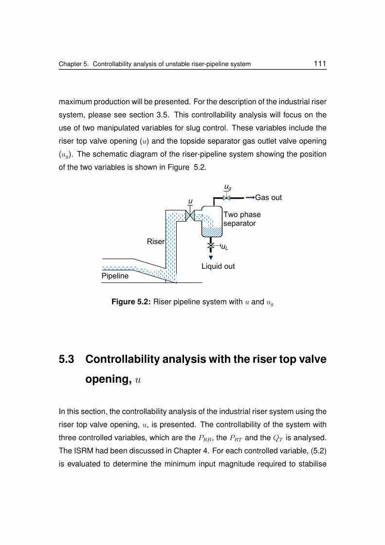
Chapter 5. Controllability analysis of unstable riser-pipeline system 111
maximum production will be presented. For the description of the industrial riser
system, please see section 3.5. This controllability analysis will focus on the
use of two manipulated variables for slug control. These variables include the
riser top valve opening (u) and the topside separator gas outlet valve opening
(ug). The schematic diagram of the riser-pipeline system showing the position
of the two variables is shown in Figure 5.2.
Two phaseseparator
Liquid out
Gas out
uLRiser
Pipeline
ug
u
Figure 5.2: Riser pipeline system with u and ug
5.3 Controllability analysis with the riser top valve
opening, u
In this section, the controllability analysis of the industrial riser system using the
riser top valve opening, u, is presented. The controllability of the system with
three controlled variables, which are the PRB, the PRT and the QT is analysed.
The ISRM had been discussed in Chapter 4. For each controlled variable, (5.2)
is evaluated to determine the minimum input magnitude required to stabilise
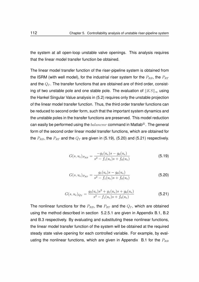
112 Chapter 5. Controllability analysis of unstable riser-pipeline system
the system at all open-loop unstable valve openings. This analysis requires
that the linear model transfer function be obtained.
The linear model transfer function of the riser-pipeline system is obtained from
the ISRM (with well model), for the industrial riser system for the PRB, the PRTand the QT . The transfer functions that are obtained are of third order, consist-
ing of two unstable pole and one stable pole. The evaluation of ‖KS‖∞ using
the Hankel Singular Value analysis in (5.2) requires only the unstable projection
of the linear model transfer function. Thus, the third order transfer functions can
be reduced to second order form, such that the important system dynamics and
the unstable poles in the transfer functions are preserved. This model reduction
can easily be performed using the balancmr command in Matlabr. The general
form of the second order linear model transfer functions, which are obtained for
the PRB, the PRT and the QT are given in (5.19), (5.20) and (5.21) respectively.
G(s, ue)PRB =−g1(ue)s− g0(ue)
s2 − f1(ue)s+ f0(ue)(5.19)
G(s, ue)PRT =g1(ue)s− g0(ue)
s2 − f1(ue)s+ f0(ue)(5.20)
G(s, ue)QT =g2(ue)s
2 + g1(ue)s+ g0(ue)
s2 − f1(ue)s+ f0(ue)(5.21)
The nonlinear functions for the PRB, the PRT and the QT , which are obtained
using the method described in section 5.2.5.1 are given in Appendix B.1, B.2
and B.3 respectively. By evaluating and substituting these nonlinear functions,
the linear model transfer function of the system will be obtained at the required
steady state valve opening for each controlled variable. For example, by eval-
uating the nonlinear functions, which are given in Appendix B.1 for the PRB
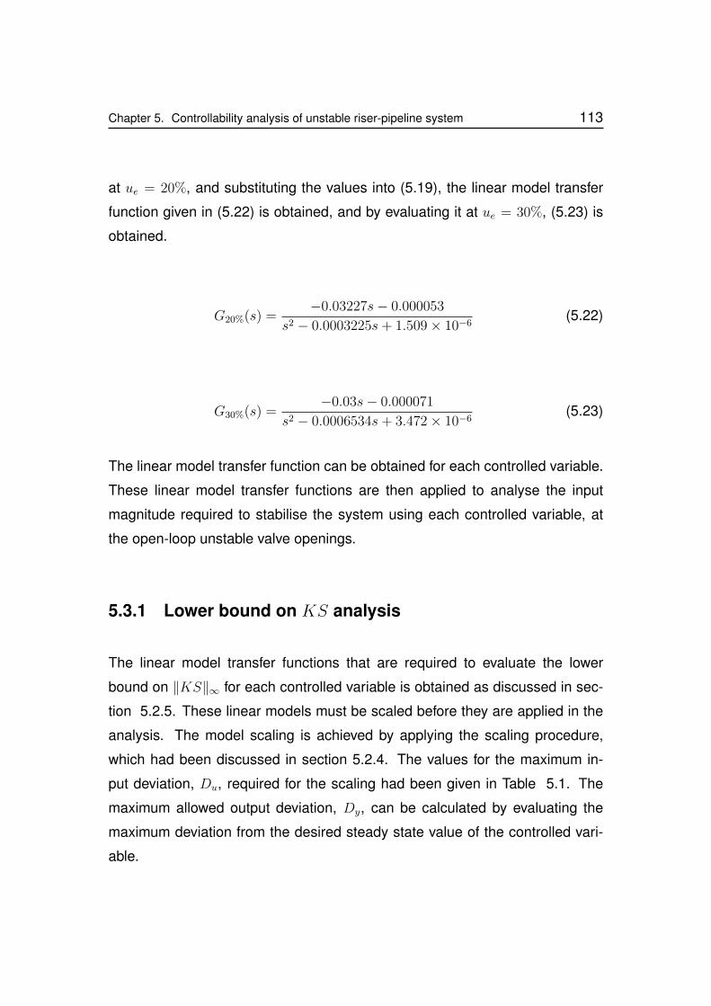
Chapter 5. Controllability analysis of unstable riser-pipeline system 113
at ue = 20%, and substituting the values into (5.19), the linear model transfer
function given in (5.22) is obtained, and by evaluating it at ue = 30%, (5.23) is
obtained.
G20%(s) =−0.03227s− 0.000053
s2 − 0.0003225s+ 1.509× 10⁻⁶(5.22)
G30%(s) =−0.03s− 0.000071
s2 − 0.0006534s+ 3.472× 10⁻⁶(5.23)
The linear model transfer function can be obtained for each controlled variable.
These linear model transfer functions are then applied to analyse the input
magnitude required to stabilise the system using each controlled variable, at
the open-loop unstable valve openings.
5.3.1 Lower bound on KS analysis
The linear model transfer functions that are required to evaluate the lower
bound on ‖KS‖∞ for each controlled variable is obtained as discussed in sec-
tion 5.2.5. These linear models must be scaled before they are applied in the
analysis. The model scaling is achieved by applying the scaling procedure,
which had been discussed in section 5.2.4. The values for the maximum in-
put deviation, Du, required for the scaling had been given in Table 5.1. The
maximum allowed output deviation, Dy, can be calculated by evaluating the
maximum deviation from the desired steady state value of the controlled vari-
able.
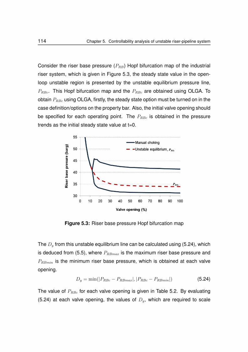
114 Chapter 5. Controllability analysis of unstable riser-pipeline system
Consider the riser base pressure (PRB) Hopf bifurcation map of the industrial
riser system, which is given in Figure 5.3, the steady state value in the open-
loop unstable region is presented by the unstable equilibrium pressure line,
PRBc. This Hopf bifurcation map and the PRBc are obtained using OLGA. To
obtain PRBc using OLGA, firstly, the steady state option must be turned on in the
case definition/options on the property bar. Also, the initial valve opening should
be specified for each operating point. The PRBc is obtained in the pressure
trends as the initial steady state value at t=0.
PRBc
, PRBc
Figure 5.3: Riser base pressure Hopf bifurcation map
The Dy from this unstable equilibrium line can be calculated using (5.24), which
is deduced from (5.5), where PRBmax is the maximum riser base pressure and
PRBmin is the minimum riser base pressure, which is obtained at each valve
opening.
Dy = min(|PRBc − PRBmax|, |PRBc − PRBmin|) (5.24)
The value of PRBc for each valve opening is given in Table 5.2. By evaluating
(5.24) at each valve opening, the values of Dy, which are required to scale
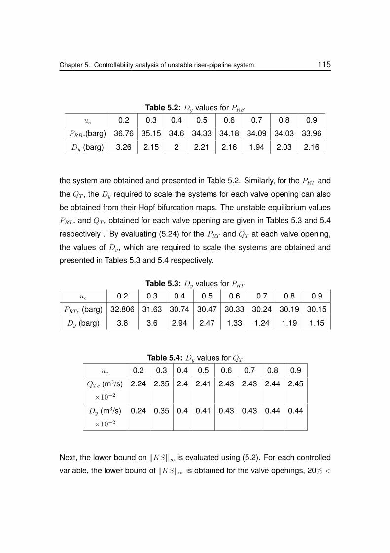
Chapter 5. Controllability analysis of unstable riser-pipeline system 115
Table 5.2: Dy values for PRBue 0.2 0.3 0.4 0.5 0.6 0.7 0.8 0.9
PRBc(barg) 36.76 35.15 34.6 34.33 34.18 34.09 34.03 33.96
Dy (barg) 3.26 2.15 2 2.21 2.16 1.94 2.03 2.16
the system are obtained and presented in Table 5.2. Similarly, for the PRT and
the QT , the Dy required to scale the systems for each valve opening can also
be obtained from their Hopf bifurcation maps. The unstable equilibrium values
PRTc and QTc obtained for each valve opening are given in Tables 5.3 and 5.4
respectively . By evaluating (5.24) for the PRT and QT at each valve opening,
the values of Dy, which are required to scale the systems are obtained and
presented in Tables 5.3 and 5.4 respectively.
Table 5.3: Dy values for PRTue 0.2 0.3 0.4 0.5 0.6 0.7 0.8 0.9
PRTc (barg) 32.806 31.63 30.74 30.47 30.33 30.24 30.19 30.15
Dy (barg) 3.8 3.6 2.94 2.47 1.33 1.24 1.19 1.15
Table 5.4: Dy values for QT
ue 0.2 0.3 0.4 0.5 0.6 0.7 0.8 0.9
QTc (m3/s) 2.24 2.35 2.4 2.41 2.43 2.43 2.44 2.45
×10−2
Dy (m3/s) 0.24 0.35 0.4 0.41 0.43 0.43 0.44 0.44
×10−2
Next, the lower bound on ‖KS‖∞ is evaluated using (5.2). For each controlled
variable, the lower bound of ‖KS‖∞ is obtained for the valve openings, 20% <
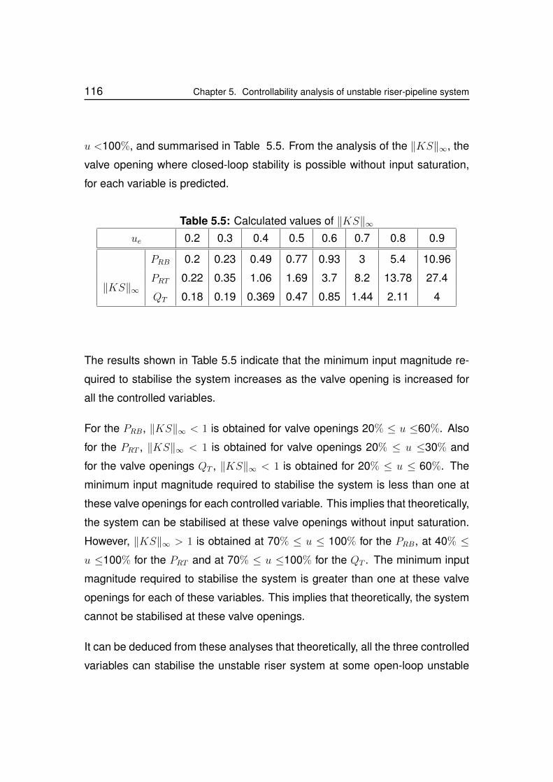
116 Chapter 5. Controllability analysis of unstable riser-pipeline system
u <100%, and summarised in Table 5.5. From the analysis of the ‖KS‖∞, the
valve opening where closed-loop stability is possible without input saturation,
for each variable is predicted.
Table 5.5: Calculated values of ‖KS‖∞ue 0.2 0.3 0.4 0.5 0.6 0.7 0.8 0.9
‖KS‖∞
PRB 0.2 0.23 0.49 0.77 0.93 3 5.4 10.96
PRT 0.22 0.35 1.06 1.69 3.7 8.2 13.78 27.4
QT 0.18 0.19 0.369 0.47 0.85 1.44 2.11 4
The results shown in Table 5.5 indicate that the minimum input magnitude re-
quired to stabilise the system increases as the valve opening is increased for
all the controlled variables.
For the PRB, ‖KS‖∞ < 1 is obtained for valve openings 20% ≤ u ≤60%. Also
for the PRT , ‖KS‖∞ < 1 is obtained for valve openings 20% ≤ u ≤30% and
for the valve openings QT , ‖KS‖∞ < 1 is obtained for 20% ≤ u ≤ 60%. The
minimum input magnitude required to stabilise the system is less than one at
these valve openings for each controlled variable. This implies that theoretically,
the system can be stabilised at these valve openings without input saturation.
However, ‖KS‖∞ > 1 is obtained at 70% ≤ u ≤ 100% for the PRB, at 40% ≤u ≤100% for the PRT and at 70% ≤ u ≤100% for the QT . The minimum input
magnitude required to stabilise the system is greater than one at these valve
openings for each of these variables. This implies that theoretically, the system
cannot be stabilised at these valve openings.
It can be deduced from these analyses that theoretically, all the three controlled
variables can stabilise the unstable riser system at some open-loop unstable
Chapter 5. Controllability analysis of unstable riser-pipeline system 117
valve opening without input saturation. However, the important issue resulting
from the controllability analysis of these variables is that the maximum stable
valve opening, which they can each achieve is different. Generally, it can be
observed that the PRB and the QT are able to stabilise the system at a larger
valve opening than the PRT . This is important as it reflects the production that
is achievable with each controlled variable, under stable operating condition.
Having analysed the controllability of the unstable riser-pipeline system with
riser top valve as the manipulated, next the controllability analysis is performed
with the topside separator gas valve as the manipulated variable.
5.4 Controllability analysis with the topside sepa-
rator gas valve ug
In this section, the controllability analysis of the industrial riser system (with well
and separator models) using the topside separator gas valve opening is pre-
sented (see Figure 5.2). The topside separator is modeled with the dimension
of the two phase separator given in Figure 4.3. The focus of the controllability
analysis will be on four controlled variables, which include the PRB, the separa-
tor pressure (Ps), the PRT and the volumetric gas flowrate out of the separator,
QGouts. For a better understanding of the stability behaviour of the system with
ug, firstly, the nonlinear stability analysis of the system will be presented.
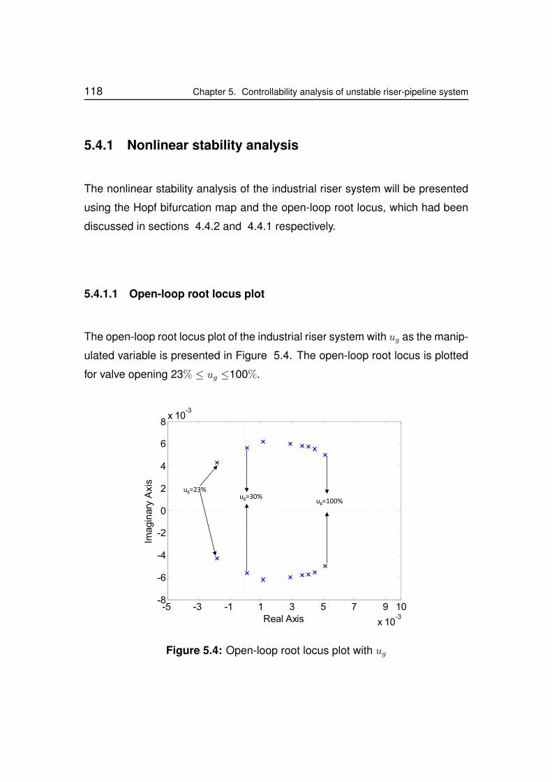
118 Chapter 5. Controllability analysis of unstable riser-pipeline system
5.4.1 Nonlinear stability analysis
The nonlinear stability analysis of the industrial riser system will be presented
using the Hopf bifurcation map and the open-loop root locus, which had been
discussed in sections 4.4.2 and 4.4.1 respectively.
5.4.1.1 Open-loop root locus plot
The open-loop root locus plot of the industrial riser system with ug as the manip-
ulated variable is presented in Figure 5.4. The open-loop root locus is plotted
for valve opening 23% ≤ ug ≤100%.
-5 -3 -1 1 3 5 7 9 10
x 10-3
-8
-6
-4
-2
0
2
4
6
8x 10
-3
Real Axis
Imagin
ary
Axis
ug=100%ug=30%
ug=23%
Figure 5.4: Open-loop root locus plot with ug
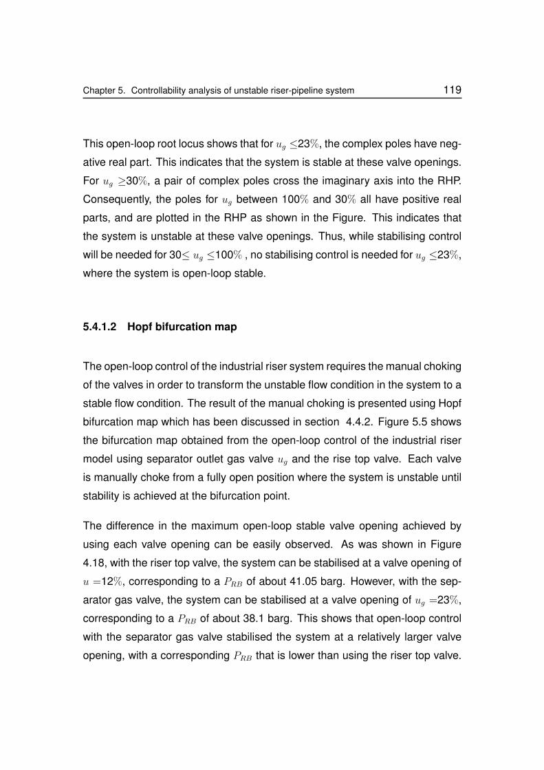
Chapter 5. Controllability analysis of unstable riser-pipeline system 119
This open-loop root locus shows that for ug ≤23%, the complex poles have neg-
ative real part. This indicates that the system is stable at these valve openings.
For ug ≥30%, a pair of complex poles cross the imaginary axis into the RHP.
Consequently, the poles for ug between 100% and 30% all have positive real
parts, and are plotted in the RHP as shown in the Figure. This indicates that
the system is unstable at these valve openings. Thus, while stabilising control
will be needed for 30≤ ug ≤100% , no stabilising control is needed for ug ≤23%,
where the system is open-loop stable.
5.4.1.2 Hopf bifurcation map
The open-loop control of the industrial riser system requires the manual choking
of the valves in order to transform the unstable flow condition in the system to a
stable flow condition. The result of the manual choking is presented using Hopf
bifurcation map which has been discussed in section 4.4.2. Figure 5.5 shows
the bifurcation map obtained from the open-loop control of the industrial riser
model using separator outlet gas valve ug and the rise top valve. Each valve
is manually choke from a fully open position where the system is unstable until
stability is achieved at the bifurcation point.
The difference in the maximum open-loop stable valve opening achieved by
using each valve opening can be easily observed. As was shown in Figure
4.18, with the riser top valve, the system can be stabilised at a valve opening of
u =12%, corresponding to a PRB of about 41.05 barg. However, with the sep-
arator gas valve, the system can be stabilised at a valve opening of ug =23%,
corresponding to a PRB of about 38.1 barg. This shows that open-loop control
with the separator gas valve stabilised the system at a relatively larger valve
opening, with a corresponding PRB that is lower than using the riser top valve.
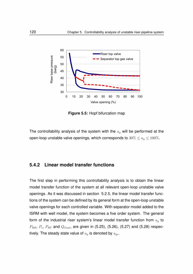
120 Chapter 5. Controllability analysis of unstable riser-pipeline system
30
35
40
45
50
55
60
0 10 20 30 40 50 60 70 80 90 100
Ris
er
ba
sep
ress
ure
(ba
rg)
Valve opening (%)
Riser top valve
Separator top gas valve
Figure 5.5: Hopf bifurcation map
The controllability analysis of the system with the ug will be performed at the
open-loop unstable valve openings, which corresponds to 30% ≤ ug ≤ 100%.
5.4.2 Linear model transfer functions
The first step in performing this controllability analysis is to obtain the linear
model transfer function of the system at all relevant open-loop unstable valve
openings. As it was discussed in section 5.2.5, the linear model transfer func-
tions of the system can be defined by its general form at the open-loop unstable
valve openings for each controlled variable. With separator model added to the
ISRM with well model, the system becomes a five order system. The general
form of the industrial riser system’s linear model transfer function from ug to
PRB, Ps, PRT and QGouts are given in (5.25), (5.26), (5.27) and (5.28) respec-
tively. The steady state value of ug is denoted by uge.
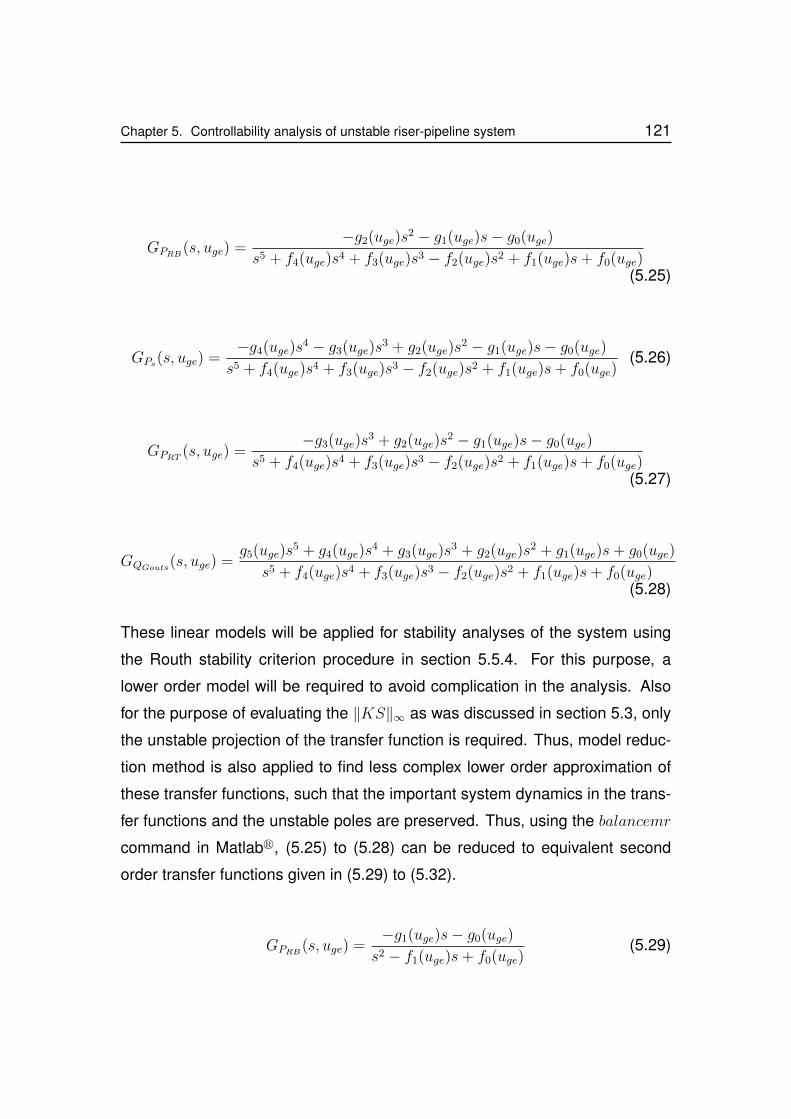
Chapter 5. Controllability analysis of unstable riser-pipeline system 121
GPRB(s, uge) =−g2(uge)s
2 − g1(uge)s− g0(uge)
s5 + f4(uge)s4 + f3(uge)s3 − f2(uge)s2 + f1(uge)s+ f0(uge)(5.25)
GPs(s, uge) =−g4(uge)s
4 − g3(uge)s3 + g2(uge)s
2 − g1(uge)s− g0(uge)
s5 + f4(uge)s4 + f3(uge)s3 − f2(uge)s2 + f1(uge)s+ f0(uge)(5.26)
GPRT (s, uge) =−g3(uge)s
3 + g2(uge)s2 − g1(uge)s− g0(uge)
s5 + f4(uge)s4 + f3(uge)s3 − f2(uge)s2 + f1(uge)s+ f0(uge)(5.27)
GQGouts(s, uge) =g5(uge)s
5 + g4(uge)s4 + g3(uge)s
3 + g2(uge)s2 + g1(uge)s+ g0(uge)
s5 + f4(uge)s4 + f3(uge)s3 − f2(uge)s2 + f1(uge)s+ f0(uge)(5.28)
These linear models will be applied for stability analyses of the system using
the Routh stability criterion procedure in section 5.5.4. For this purpose, a
lower order model will be required to avoid complication in the analysis. Also
for the purpose of evaluating the ‖KS‖∞ as was discussed in section 5.3, only
the unstable projection of the transfer function is required. Thus, model reduc-
tion method is also applied to find less complex lower order approximation of
these transfer functions, such that the important system dynamics in the trans-
fer functions and the unstable poles are preserved. Thus, using the balancemr
command in Matlabr, (5.25) to (5.28) can be reduced to equivalent second
order transfer functions given in (5.29) to (5.32).
GPRB(s, uge) =−g1(uge)s− g0(uge)
s2 − f1(uge)s+ f0(uge)(5.29)
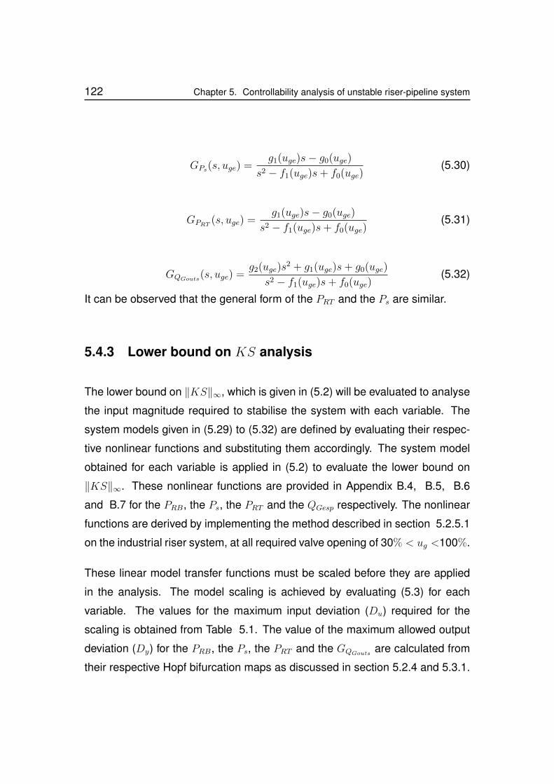
122 Chapter 5. Controllability analysis of unstable riser-pipeline system
GPs(s, uge) =g1(uge)s− g0(uge)
s2 − f1(uge)s+ f0(uge)(5.30)
GPRT (s, uge) =g1(uge)s− g0(uge)
s2 − f1(uge)s+ f0(uge)(5.31)
GQGouts(s, uge) =g2(uge)s
2 + g1(uge)s+ g0(uge)
s2 − f1(uge)s+ f0(uge)(5.32)
It can be observed that the general form of the PRT and the Ps are similar.
5.4.3 Lower bound on KS analysis
The lower bound on ‖KS‖∞, which is given in (5.2) will be evaluated to analyse
the input magnitude required to stabilise the system with each variable. The
system models given in (5.29) to (5.32) are defined by evaluating their respec-
tive nonlinear functions and substituting them accordingly. The system model
obtained for each variable is applied in (5.2) to evaluate the lower bound on
‖KS‖∞. These nonlinear functions are provided in Appendix B.4, B.5, B.6
and B.7 for the PRB, the Ps, the PRT and the QGesp respectively. The nonlinear
functions are derived by implementing the method described in section 5.2.5.1
on the industrial riser system, at all required valve opening of 30% < ug <100%.
These linear model transfer functions must be scaled before they are applied
in the analysis. The model scaling is achieved by evaluating (5.3) for each
variable. The values for the maximum input deviation (Du) required for the
scaling is obtained from Table 5.1. The value of the maximum allowed output
deviation (Dy) for the PRB, the Ps, the PRT and the GQGouts are calculated from
their respective Hopf bifurcation maps as discussed in section 5.2.4 and 5.3.1.
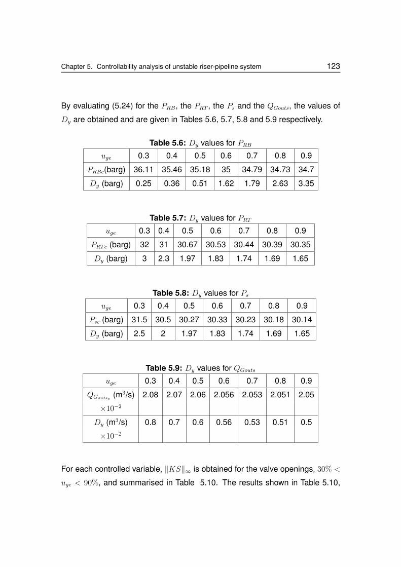
Chapter 5. Controllability analysis of unstable riser-pipeline system 123
By evaluating (5.24) for the PRB, the PRT , the Ps and the QGouts, the values of
Dy are obtained and are given in Tables 5.6, 5.7, 5.8 and 5.9 respectively.
Table 5.6: Dy values for PRBuge 0.3 0.4 0.5 0.6 0.7 0.8 0.9
PRBc(barg) 36.11 35.46 35.18 35 34.79 34.73 34.7
Dy (barg) 0.25 0.36 0.51 1.62 1.79 2.63 3.35
Table 5.7: Dy values for PRTuge 0.3 0.4 0.5 0.6 0.7 0.8 0.9
PRTc (barg) 32 31 30.67 30.53 30.44 30.39 30.35
Dy (barg) 3 2.3 1.97 1.83 1.74 1.69 1.65
Table 5.8: Dy values for Psuge 0.3 0.4 0.5 0.6 0.7 0.8 0.9
Psc (barg) 31.5 30.5 30.27 30.33 30.23 30.18 30.14
Dy (barg) 2.5 2 1.97 1.83 1.74 1.69 1.65
Table 5.9: Dy values for QGouts
uge 0.3 0.4 0.5 0.6 0.7 0.8 0.9
QGoutsc (m3/s) 2.08 2.07 2.06 2.056 2.053 2.051 2.05
×10−2
Dy (m3/s) 0.8 0.7 0.6 0.56 0.53 0.51 0.5
×10−2
For each controlled variable, ‖KS‖∞ is obtained for the valve openings, 30% <
uge < 90%, and summarised in Table 5.10. The results shown in Table 5.10,
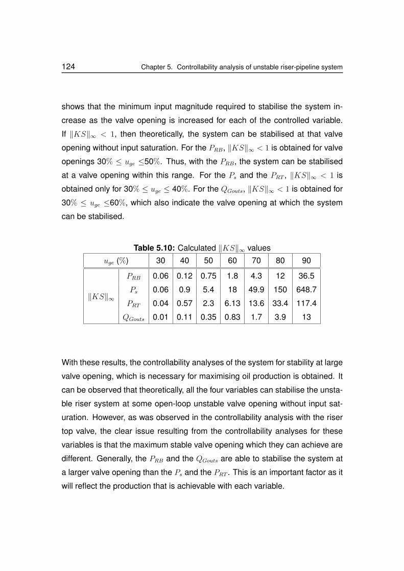
124 Chapter 5. Controllability analysis of unstable riser-pipeline system
shows that the minimum input magnitude required to stabilise the system in-
crease as the valve opening is increased for each of the controlled variable.
If ‖KS‖∞ < 1, then theoretically, the system can be stabilised at that valve
opening without input saturation. For the PRB, ‖KS‖∞ < 1 is obtained for valve
openings 30% ≤ uge ≤50%. Thus, with the PRB, the system can be stabilised
at a valve opening within this range. For the Ps and the PRT , ‖KS‖∞ < 1 is
obtained only for 30% ≤ uge ≤ 40%. For the QGouts, ‖KS‖∞ < 1 is obtained for
30% ≤ uge ≤60%, which also indicate the valve opening at which the system
can be stabilised.
Table 5.10: Calculated ‖KS‖∞ values
uge (%) 30 40 50 60 70 80 90
‖KS‖∞
PRB 0.06 0.12 0.75 1.8 4.3 12 36.5
Ps 0.06 0.9 5.4 18 49.9 150 648.7
PRT 0.04 0.57 2.3 6.13 13.6 33.4 117.4
QGouts 0.01 0.11 0.35 0.83 1.7 3.9 13
With these results, the controllability analyses of the system for stability at large
valve opening, which is necessary for maximising oil production is obtained. It
can be observed that theoretically, all the four variables can stabilise the unsta-
ble riser system at some open-loop unstable valve opening without input sat-
uration. However, as was observed in the controllability analysis with the riser
top valve, the clear issue resulting from the controllability analyses for these
variables is that the maximum stable valve opening which they can achieve are
different. Generally, the PRB and the QGouts are able to stabilise the system at
a larger valve opening than the Ps and the PRT . This is an important factor as it
will reflect the production that is achievable with each variable.
Chapter 5. Controllability analysis of unstable riser-pipeline system 125
5.5 Simulations and results analyses
In the controllability analysis with the riser top valve opening (u), it was found
generally that the PRB and the QT are able to stabilise the system at a larger
valve opening than the PRT . Also, in the controllability analysis with the sepa-
rator gas valve (ug), it was found that generally the PRB and the QGouts are able
to stabilise the system at a larger valve opening than the Ps and the PRT . In the
practical implementation of slug control system, the ability to achieve closed-
loop stability at the predicted valve opening will depend on a number of factors,
including the appropriateness of the slug control structure. In this section, a
feedback control structure with derivative controller (D controller) is applied on
the industrial riser system to validate the general prediction of the controllability
analyses results.
5.5.1 The simulation model
The controller parameters are designed with linear model transfer function,
which is obtained from the ISRM of the industrial riser system. The industrial
riser system was described in section 3.5. The controller is then implemented
on the industrial riser system, which is modeled in the OLGA multiphase flow
simulator software. The OLGA model of the industrial riser system is nonlin-
ear. The implementation of the controller is achieved using the OLGA-Matlab
link, which is established by using the OLGA-Matlab toolbox. The controller
is configured in the Matlabr software. Through OLGA-Matlab link, the results
(controlled variable data) from dynamic multiphase flow simulations performed
by OLGA becomes available in MATLAB, and the control input from Matlab
become available in OLGA.
126 Chapter 5. Controllability analysis of unstable riser-pipeline system
5.5.2 Control structure with derivative controller
The control structure that allows the practical application of the slug control sys-
tem to focus on stabilising the system at a reference valve opening, will be dis-
cussed and applied on the industrial riser system. A feedback control structure
with derivative controller (D controller) is proposed for this purpose. Consider
the general relationship for a derivative controller in which the controller input
is the control error (e), as shown in (5.33).
u(t) = Kcτdde(t)
dt(5.33)
In (5.33), Kc is the controller gain, e(t) is the control error and τd is the derivative
time. Fundamentally, the control action of the derivative controller is obtained
by taking the derivative of the control error, which is the controller input. If the
control error becomes constant (not necessarily zero), the derivative controller
output will be zero. For a stable riser system, the controlled variable will be
fairly constant. Thus, if the controller input is equal to the measured value of
the controlled variable, then, the derivative controller can be applied to stabilise
the system, such that, for a stable system (steady state), the controller output
will be equal to zero. In this case, the controlled variable set point can be set
equal to zero, such that the controller input will be equal to the measured value
of the controlled variable, as shown in Figure 5.6. This slug control strategy
eliminates the requirement for perfect tracking of the controlled variable as a
slug control objective, which does not provide any benefit to the slug control of
the oil and gas production system.
Since the controller output will be approximately equal to zero (uk ≈ 0) for
a constant value of the controlled variable (at steady state), then a reference
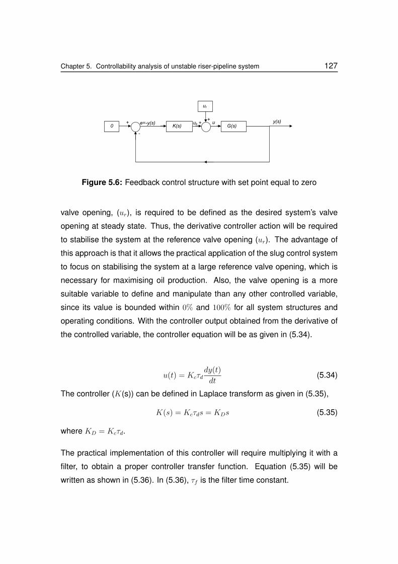
Chapter 5. Controllability analysis of unstable riser-pipeline system 127
e=-y(s)G(s)K(s)
ur
+
-
uk u y(s)++
0
Figure 5.6: Feedback control structure with set point equal to zero
valve opening, (ur), is required to be defined as the desired system’s valve
opening at steady state. Thus, the derivative controller action will be required
to stabilise the system at the reference valve opening (ur). The advantage of
this approach is that it allows the practical application of the slug control system
to focus on stabilising the system at a large reference valve opening, which is
necessary for maximising oil production. Also, the valve opening is a more
suitable variable to define and manipulate than any other controlled variable,
since its value is bounded within 0% and 100% for all system structures and
operating conditions. With the controller output obtained from the derivative of
the controlled variable, the controller equation will be as given in (5.34).
u(t) = Kcτddy(t)
dt(5.34)
The controller (K(s)) can be defined in Laplace transform as given in (5.35),
K(s) = Kcτds = KDs (5.35)
where KD = Kcτd.
The practical implementation of this controller will require multiplying it with a
filter, to obtain a proper controller transfer function. Equation (5.35) will be
written as shown in (5.36). In (5.36), τf is the filter time constant.
128 Chapter 5. Controllability analysis of unstable riser-pipeline system
K(s) =KDs
τfs+ 1(5.36)
The implementation of this controller will first require the determination of its
parameters. In order to determine the values of KD and τf for which the system
is stable, a system stability analysis method is applied. One of such methods
is the Routh stability criterion. The Routh stability criterion is discussed briefly
in the next section.
5.5.2.1 Routh stability criterion
In this section, the a popular system stability analysis tool, known as the Routh
stability criterion will be introduced. The Routh stability criterion states that the
number of polynomial roots in the right-half-plane (RHP) ( i.e RHP poles) of the
S-plane is equal to the number of sign changes in the first column of the Routh
array table [81]. It is known that the presence of RHP poles indicates unstable
system [74]. Thus, any sign change in the first column of the Routh array table
would indicate that the system is unstable. The Routh stability criterion can
be used to evaluate the limits of the magnitude of the controller parameters for
which the element in the first column of the Routh array table would be positive.
The Routh stability criterion is applied to the characteristic equation of a closed-
loop transfer function of the system defined by, 1 + G(s)K(s) = 0, where G(s)
is the system transfer function and K(s) is the controller. The coefficients of
this closed-loop transfer function are applied to create the Routh array table
from which the analysis is performed. The mathematical steps for analysing
the Routh array table is defined in the literature [74, 81].
Chapter 5. Controllability analysis of unstable riser-pipeline system 129
5.5.3 Simulation with riser top valve (u) as manipulated vari-
able
The simulation analyses with the riser top valve as the manipulated variable
is presented in this section. In line with the controllability analysis, simulation
analyses for three controlled variables namely the PRB, the PRT and the QT
are presented. The derivative controller will be designed for each controlled
variable using the linear model transfer function obtained from the ISRM. The
controller is then implemented on the nonlinear model of the industrial riser
system in OLGA as described in section 5.5.1.
5.5.3.1 Simulation procedure
For each controlled variable, the following procedure is followed in performing
the simulation to implement the controller.
1. The valve opening is initially set to a fixed position (manually) correspond-
ing to the open-loop unstable valve opening of u =20%.
2. The controller is switched on after open-loop simulation period that is
greater than 2 hours and the system is allowed to be stabilised by the
controller action.
3. Once the system is stabilised, the reference valve opening (ur) is gradu-
ally increased and the system is allowed to be stabilise by the controller
action for each step increase.
130 Chapter 5. Controllability analysis of unstable riser-pipeline system
4. The gradual increase in the ur is continued until the valve opening at
which the controller cannot stabilise the system is reached. At this valve
opening, the system becomes unstable.
5. The maximum stable valve opening, the minimum PRB and the accumu-
lated liquid achieved is then recorded.
It will be observed that based on this simulation procedure, in each simulation
result, the system oscillates at the beginning of the simulation because the
system is open-loop unstable and also oscillates at the end because the system
is closed-loop unstable. This simulation procedure applies to all the simulation
results presented in sections 5.5.3.2, 5.5.3.3, 5.5.3.4 and 5.5.4.
5.5.3.2 PRB control
To obtain the bounds for the values of KD and τf for which the system is sta-
ble at any valve opening, the Routh stability analysis will be applied using the
system’s model given in (5.19). With the PRB, the closed-loop characteristic
equation of the system is obtained as 1−G(s, ue)K(s) = 0. With the K(s) given
as the derivative controller in (5.36), the characteristic equation is be obtained
as shown in (5.37).
τfs3 + s2[g1(ue)KD − f1(ue)τf + 1] + s[g0(ue)KD − f1(ue) + τff0(ue)] + f0(ue) = 0
(5.37)
From (5.37), the Routh array table, which is shown in Table 5.11 is created.
where S11 =AK2
D+BKD+C
g1(ue)KD−f1(ue)τf+1and
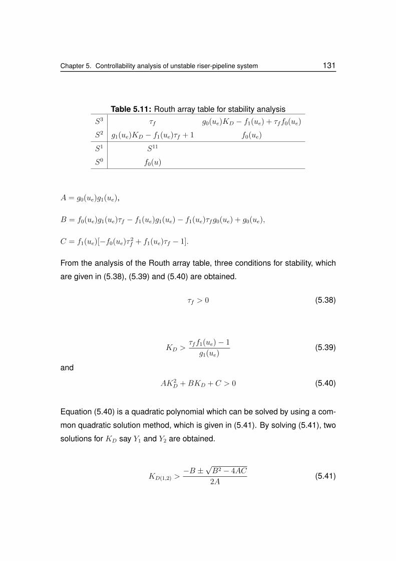
Chapter 5. Controllability analysis of unstable riser-pipeline system 131
Table 5.11: Routh array table for stability analysisS3 τf g0(ue)KD − f1(ue) + τff0(ue)
S2 g1(ue)KD − f1(ue)τf + 1 f0(ue)
S1 S11
S0 f0(u)
A = g0(ue)g1(ue),
B = f0(ue)g1(ue)τf − f1(ue)g1(ue)− f1(ue)τfg0(ue) + g0(ue),
C = f1(ue)[−f0(ue)τ2f + f1(ue)τf − 1].
From the analysis of the Routh array table, three conditions for stability, which
are given in (5.38), (5.39) and (5.40) are obtained.
τf > 0 (5.38)
KD >τff1(ue)− 1
g1(ue)(5.39)
and
AK2D +BKD + C > 0 (5.40)
Equation (5.40) is a quadratic polynomial which can be solved by using a com-
mon quadratic solution method, which is given in (5.41). By solving (5.41), two
solutions for KD say Y1 and Y2 are obtained.
KD(1,2) >−B ±
√B2 − 4AC
2A(5.41)
132 Chapter 5. Controllability analysis of unstable riser-pipeline system
The solution for KD from (5.41) will be obtained by evaluating (5.42).
KD > max(Y1, Y2) (5.42)
Through the numerical evaluation of these conditions using the nonlinear func-
tions, which are given in (B.1) to (B.4) in Appendix B.1, the solutions from (5.39)
and (5.42) are combined to obtained (5.43), which gives the combined solution
for the value of KD for which the system will be stable.
KD > Y1, Y1 =−B +
√B2 − 4AC
2A(5.43)
Stability condition analyses
For robust stability of the system, it is desired that the controller be designed
at the valve opening which require small control input to achieve stability. By
analysing (5.43) for the PRB, it is observed that generally, the lower bound of
KD required to stabilise the system will increase with increasing values of f1(ue)
and decreasing value of the product of the open-loop transfer function numer-
ator coefficients, g1(ue) and g0(ue). Thus, for large values of f1(ue) and small
values of g1(ue)g0(ue), the control input required to stabilise the system will be
large, a condition which is not suitable for achieving robust stability in the sys-
tem. Small value of KD can be achieved at a valve opening with relatively small
values of f1(ue) and large values of g1(ue)g0(ue), when compared to other valve
openings. With this insight, the operating condition of the system and the sys-
tem design can be defined to satisfy these condition in the open-loop transfer
function.

Chapter 5. Controllability analysis of unstable riser-pipeline system 133
Controller synthesis and simulation results
By evaluating the nonlinear functions and applying them on (5.43), the lower
bound of the value of KD for which the system will be stable for each valve
opening is evaluated. The value of the filter time constant (τf ) is defined to be
equal to 0.9. The obtained values are summarised in Table 5.12.
Table 5.12: Calculated KD values for the PRBue (%) 20 30 40 50 60 70 80 90 100
KD(s/barg)(>) 6.1 9.2 25.4 38.7 56.3 73.1 74.6 75.4 76.8
From Table 5.12, the effect of the system’s valve opening on the magnitude
of KD required for stability can be observed. Generally, the magnitude of KD
required to achieve stability increases as the valve opening increases. This
reflects the increasing magnitude of the control input that is required to sta-
bilise the system as the open-loop valve opening increases. This agrees with
the result of the controllability analysis (see Table 5.5). For a small value of
ue, the KD is relatively small, indicating that relatively small control input will
be required to stabilise the system at this valve opening, a condition which is
necessary for achieving robust stability in the system.
The controller designed at u = 20% is therefore implemented and the simulation
results obtained is analysed. The controller value implemented in the simulation
is obtained by multiplying the minimum value, which is given in Table 5.12 by a
factor of 2(6dB). The value of the filter time constant (τf ) is defined to be equal
to 0.9.
During the simulation the following steps are taken in line with the procedure
explained in section 5.5.3.

134 Chapter 5. Controllability analysis of unstable riser-pipeline system
1. The valve opening is initially set to a fixed position corresponding to the
open-loop unstable valve opening of u =20%.
2. The controller is then switched on after a simulation period of 4 hours. It
is observed that the system is stabilised when the controller is switched
on.
3. Once the system is stabilised, the reference valve opening (ur) is grad-
ually increased and the system is allowed to stabilise for each step in-
crease.
4. The gradual increase in the ur is continued until the valve opening at
which the controller cannot stabilise the system is reached at 29 hours.
0 5 10 15 20 25 3030
35
40
45
50Riser base and top pressure
Pre
ssu
re(b
arg
)
0 5 10 15 20 25 300
20
40
60
80100
Valve opening
Va
lve
op
enin
g(%
)
Z Zref
PRB
PRT
0 5 10 15 20 25 300
10
20
30
40Riser top liquid flowrate
Ris
erto
pli
qu
idfl
ow
rate
(kg
/s)
Time (h)
u uref
Figure 5.7: Simulation result for the PRB
Chapter 5. Controllability analysis of unstable riser-pipeline system 135
From this simulation result, it can be observed that the system was stabilised
at a maximum valve opening of 49%. Next, the control of the system with PRTwill be presented.
5.5.3.3 PRT control
The simulation result obtained by implementing the PRT as the controlled vari-
able is also presented. The Routh stability analysis, which is similar to that
performed for the PRB can be also be applied for the PRT to obtain the con-
dition for stability. The resulting conditions for evaluating the value of KD for
which the system will be stable are given in (5.44), (5.45) and (5.46).
τf > 0 (5.44)
KD < −τff1(ue)− 1
g1(ue)(5.45)
AK2D +BKD + C > 0 (5.46)
where A = −g1(ue)g0(ue)
B = f1(ue)g1(ue)− f0(ue)g1(ue)τf − f1(ue)τfg0(ue) + g0(ue),
C = f1(ue)(f1(ue)τf − f0(ue)τ2f − 1)
Equation (5.46) is a quadratic equation, whose solution will give two conditions
for KD, say Y1 and Y2. The combined solution for KD will be better obtained
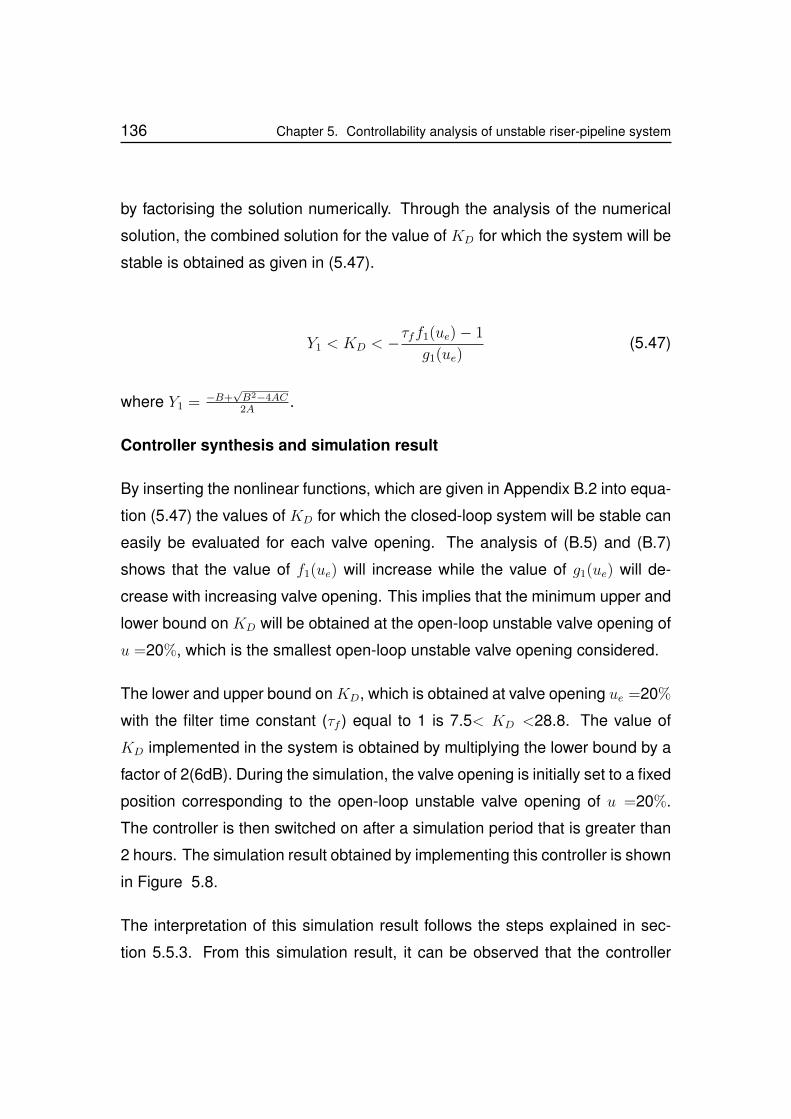
136 Chapter 5. Controllability analysis of unstable riser-pipeline system
by factorising the solution numerically. Through the analysis of the numerical
solution, the combined solution for the value of KD for which the system will be
stable is obtained as given in (5.47).
Y1 < KD < −τff1(ue)− 1
g1(ue)(5.47)
where Y1 = −B+√B2−4AC2A
.
Controller synthesis and simulation result
By inserting the nonlinear functions, which are given in Appendix B.2 into equa-
tion (5.47) the values of KD for which the closed-loop system will be stable can
easily be evaluated for each valve opening. The analysis of (B.5) and (B.7)
shows that the value of f1(ue) will increase while the value of g1(ue) will de-
crease with increasing valve opening. This implies that the minimum upper and
lower bound on KD will be obtained at the open-loop unstable valve opening of
u =20%, which is the smallest open-loop unstable valve opening considered.
The lower and upper bound onKD, which is obtained at valve opening ue =20%
with the filter time constant (τf ) equal to 1 is 7.5< KD <28.8. The value of
KD implemented in the system is obtained by multiplying the lower bound by a
factor of 2(6dB). During the simulation, the valve opening is initially set to a fixed
position corresponding to the open-loop unstable valve opening of u =20%.
The controller is then switched on after a simulation period that is greater than
2 hours. The simulation result obtained by implementing this controller is shown
in Figure 5.8.
The interpretation of this simulation result follows the steps explained in sec-
tion 5.5.3. From this simulation result, it can be observed that the controller
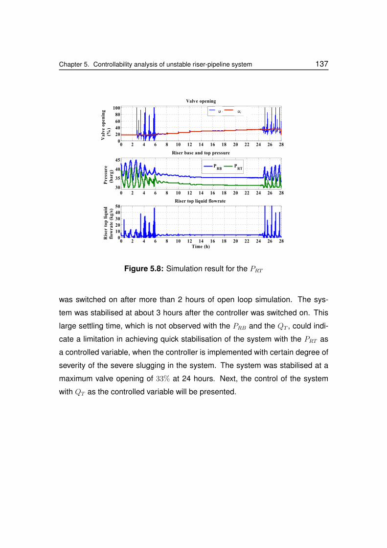
Chapter 5. Controllability analysis of unstable riser-pipeline system 137
0 2 4 6 8 10 12 14 16 18 20 22 24 26 280
20
40
60
80
100
Valve openingV
alv
eo
pen
ing
(%)
0 2 4 6 8 10 12 14 16 18 20 22 24 26 2830
35
40
45
Riser base and top pressure
Pre
ssu
re(b
arg
)
0 2 4 6 8 10 12 14 16 18 20 22 24 26 280
10
20
30
4050
Riser top liquid flowrate
Ris
erto
pli
qu
idfl
ow
rate
(kg
/s)
Time (h)
Z Zref
PRB
PRT
u uref
Figure 5.8: Simulation result for the PRT
was switched on after more than 2 hours of open loop simulation. The sys-
tem was stabilised at about 3 hours after the controller was switched on. This
large settling time, which is not observed with the PRB and the QT , could indi-
cate a limitation in achieving quick stabilisation of the system with the PRT as
a controlled variable, when the controller is implemented with certain degree of
severity of the severe slugging in the system. The system was stabilised at a
maximum valve opening of 33% at 24 hours. Next, the control of the system
with QT as the controlled variable will be presented.
138 Chapter 5. Controllability analysis of unstable riser-pipeline system
5.5.3.4 QT control
The simulation result obtained by implementing the QT as the controlled vari-
able is also presented. The Routh stability analysis, which is similar to that
performed for the PRB and the PRT can be also be applied for the QT to obtain
the condition for stability. Three conditions with which the value of KD can be
evaluated are given in (5.48), (5.49) and (5.50).
τf > −KDg2(ue) (5.48)
KD >τff1(ue)− 1
g1(ue)(5.49)
AK2D +BKD + C > 0 (5.50)
where A = g1(ue)g0(ue)
B = g1(ue)f0(ue)τf − g0(ue)τff1(ue) + g0(ue)− f1(ue)g0(ue)− f0(ue)g2(ue))
C = f1(ue)(f1(ue)τf − f0(ue)τ2f − 1)
Equation (5.50) is a quadratic equation, whose solution will give two conditions
for KD, say Y1 and Y2. The combined solution would be obtained by evaluating
(5.51). The combined solution for KD will be better obtained by factorising
the solution numerically. From the numerical solution analysis, the combined
solution for the value of KD for which the system will be stable is obtained as
given in (5.52).
Chapter 5. Controllability analysis of unstable riser-pipeline system 139
KD > max(Y1, Y2) (5.51)
KD > (Y1), Y1 =−B +
√B2 − 4AC
2A(5.52)
Controller synthesis and simulation results
By applying the nonlinear functions, which are given in Appendix B.3 to eval-
uate equation (5.52), the values of KD for which the closed-loop system will
be stable with QT as the controlled variable can easily be evaluated for each
valve opening. The condition KD > 31378 s2/m3, is obtained at valve opening
ue =20% with the filter time constant (τf ) equal to 1. The value of KD imple-
mented in the system is obtained by multiplying this minimum value by a factor
of 2(6dB). The simulation result obtained is shown in Figure 5.9.
The interpretation of this simulation result also follows the simulation proce-
dure explained in section 5.5.3. From this simulation result, it can be observed
that the system was stabilised at a maximum valve opening of 39%. Next, the
analyses and the comparison of these simulation results will be presented.
5.5.3.5 Analyses and comparison of simulated results
From the simulation results shown in Figures 5.7 - 5.9, it can be observed that
the unstable riser system was stabilised using all the three controlled variables,
at some open-loop unstable valve opening. Firstly, this shows that by applying
the control strategy implemented in this controllability analysis, any of these
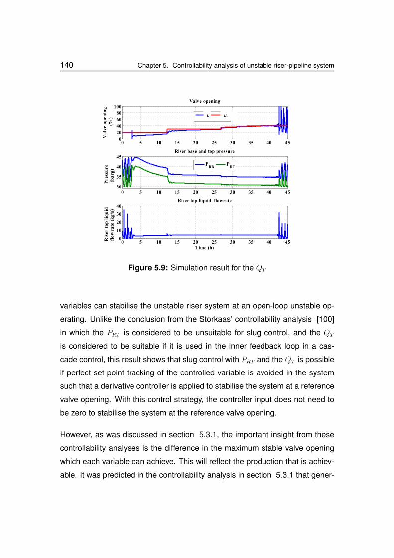
140 Chapter 5. Controllability analysis of unstable riser-pipeline system
0 5 10 15 20 25 30 35 40 450
20
40
60
80100
Va
lve
op
enin
g(%
)
Valve opening
Z Zref
0 5 10 15 20 25 30 35 40 4530
35
40
45
Pre
ssu
re(b
arg
)
Riser base and top pressure
0 5 10 15 20 25 30 35 40 450
10
20
30
40Riser top liquid flowrate
Ris
erto
pli
qu
idfl
ow
rate
(kg
/s)
Time (h)
PRB
PRT
u uref
Figure 5.9: Simulation result for the QT
variables can stabilise the unstable riser system at an open-loop unstable op-
erating. Unlike the conclusion from the Storkaas’ controllability analysis [100]
in which the PRT is considered to be unsuitable for slug control, and the QT
is considered to be suitable if it is used in the inner feedback loop in a cas-
cade control, this result shows that slug control with PRT and the QT is possible
if perfect set point tracking of the controlled variable is avoided in the system
such that a derivative controller is applied to stabilise the system at a reference
valve opening. With this control strategy, the controller input does not need to
be zero to stabilise the system at the reference valve opening.
However, as was discussed in section 5.3.1, the important insight from these
controllability analyses is the difference in the maximum stable valve opening
which each variable can achieve. This will reflect the production that is achiev-
able. It was predicted in the controllability analysis in section 5.3.1 that gener-

Chapter 5. Controllability analysis of unstable riser-pipeline system 141
ally, the PRB and the QT will stabilise the system at larger valve opening than
the PRT . From the simulation results, the PRB achieved stability at the maximum
valve opening of 49%. This is higher than that achieved with the PRT , which is
33%. Also the QT achieved stability at the maximum valve opening of 39%,
which is still higher than that achieved with the PRT . Thus, these simulation
results confirm the general trend of the ability of these variables to stabilise the
unstable riser system at large valve opening, as predicted in the controllability
analysis.
Also, the corresponding production achieved with each variable showed that the
maximum production is achieved with the PRB, while the minimum is achieved
with the PRT . These results are summarised in Table 5.13.
Table 5.13: Simulation performance tableControlled u PRBmin Production
variable (%) (barg) (m3/day)
PRB 49 34.54 348
QT 39 34.7 344.7
PRT 33 35.58 334.5
5.5.4 Simulation with topside separator gas valve (ug) as ma-
nipulated variable
The implementation of the PRB, the Ps, the PRT and the QGesp as controlled
variables to stabilise the unstable riser system with the topside separator gas
valve (ug) as manipulated variable is presented in this section. The Routh sta-
bility criterion is also applied for each variable as in the case of control with
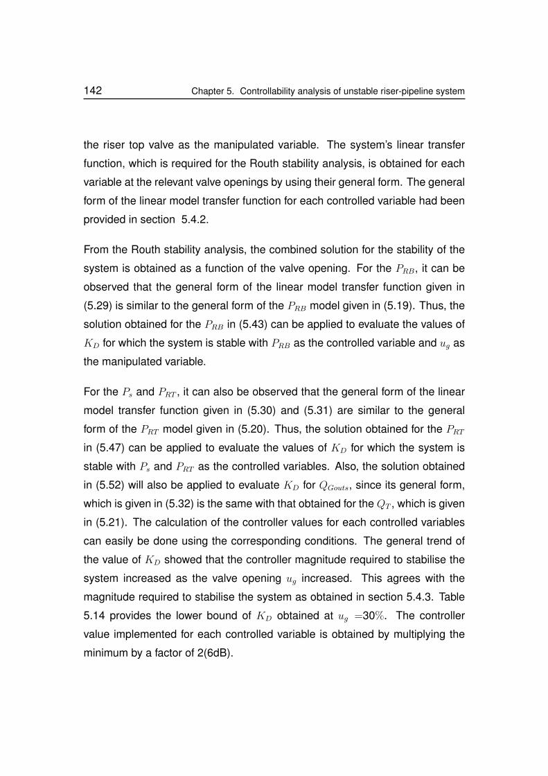
142 Chapter 5. Controllability analysis of unstable riser-pipeline system
the riser top valve as the manipulated variable. The system’s linear transfer
function, which is required for the Routh stability analysis, is obtained for each
variable at the relevant valve openings by using their general form. The general
form of the linear model transfer function for each controlled variable had been
provided in section 5.4.2.
From the Routh stability analysis, the combined solution for the stability of the
system is obtained as a function of the valve opening. For the PRB, it can be
observed that the general form of the linear model transfer function given in
(5.29) is similar to the general form of the PRB model given in (5.19). Thus, the
solution obtained for the PRB in (5.43) can be applied to evaluate the values of
KD for which the system is stable with PRB as the controlled variable and ug as
the manipulated variable.
For the Ps and PRT , it can also be observed that the general form of the linear
model transfer function given in (5.30) and (5.31) are similar to the general
form of the PRT model given in (5.20). Thus, the solution obtained for the PRT
in (5.47) can be applied to evaluate the values of KD for which the system is
stable with Ps and PRT as the controlled variables. Also, the solution obtained
in (5.52) will also be applied to evaluate KD for QGouts, since its general form,
which is given in (5.32) is the same with that obtained for the QT , which is given
in (5.21). The calculation of the controller values for each controlled variables
can easily be done using the corresponding conditions. The general trend of
the value of KD showed that the controller magnitude required to stabilise the
system increased as the valve opening ug increased. This agrees with the
magnitude required to stabilise the system as obtained in section 5.4.3. Table
5.14 provides the lower bound of KD obtained at ug =30%. The controller
value implemented for each controlled variable is obtained by multiplying the
minimum by a factor of 2(6dB).
Chapter 5. Controllability analysis of unstable riser-pipeline system 143
Table 5.14: KD values for controller designed at ug = 30%
PRB Ps PRT QGouts
KD KD > 11.1 1.8 < KD < 16.6 0.85 < KD < 12.7 KD > 27000
(s/barg) (s/barg) (s/barg) (s2/m3)
5.5.5 Simulation results analyses and comparison
In this section, the simulation result obtained from the implementation of the
controller designed for each of the controlled variable; PRB, Ps, PRT and QGouts,
is presented. For each controlled variable, the simulation results is obtained by
implementing the controller designed at ug = 30%.
The valve opening is initially set to a fixed opening corresponding to the open-
loop unstable valve opening of ug =30%. The controller is then switched on
after a simulation period when the system is open-loop unstable. Once the
system is stabilised, the reference valve opening (ur) is gradually increased
and the system is allowed to stabilise for each step increase. The gradual
increase in the ur is continued until the valve opening at which the controller
cannot stabilise the system is reached. The simulation results are presented in
Figure 5.10 - 5.13.
From these simulation results it can be observe that the system was stabilised
with all the four controlled variables when the controller was switched on. This
shows that by implementing an appropriate control strategy, any of these con-
trolled variables can stabilise the unstable riser system at an open-loop unsta-
ble operating. Thus, the key focus of the controllability analysis should be to
evaluate the maximum closed-loop stable valve opening, which each controlled
variable can achieve, since stability at a relatively large valve opening will be
144 Chapter 5. Controllability analysis of unstable riser-pipeline system
0 5 10 15 20 25 300
50
100
Valve opening
Va
lve
op
en
ing
(%)
0 5 10 15 20 25 3030
35
40
45Riser base and riser top pressure
Pre
ssu
re(b
arg
) PRB
PRT
0 5 10 15 20 25 300
10
20
30
4050
Riser top liquid flowrate
Liq
uid
flo
wra
te(k
g/s
)
Time (h)
Riser top valve Separator gas valve
Figure 5.10: Simulation result with the PRB
0 2 4 6 8 10 12 1420
40
60
80
100
Valve opening
Va
lve
op
en
ing
(%)
0 2 4 6 8 10 12 1430323436384042 Riser base and riser top pressure
Pre
ssu
re(b
arg
)
PRB
PRT
0 2 4 6 8 10 12 140
102030405060
Riser top liquid flowrate
Liq
uid
flo
wra
te(k
g/s
)
Time (h)
Riser top valve
Separator gas valve
Figure 5.11: Simulation result with the Ps
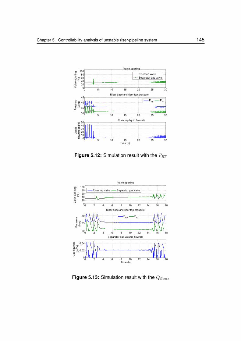
Chapter 5. Controllability analysis of unstable riser-pipeline system 145
0 5 10 15 20 25 300
20406080
100Valve opening
Va
lve
op
en
ing
(%)
0 5 10 15 20 25 3030
35
40
45Riser base and riser top pressure
Pre
ssu
re(b
arg
) PRB
PRT
0 5 10 15 20 25 300
1020304050
Riser top liquid flowrate
Liq
uid
flo
wra
te(k
g/s
)
Time (h)
Riser top valve
Separator gas valve
Figure 5.12: Simulation result with the PRT
0 2 4 6 8 10 12 14 16 180
20406080
100
Valve opening
Va
lve
op
en
ing
(%)
0 2 4 6 8 10 12 14 16 1830
35
40
Riser base and riser top pressure
Pre
ssu
re(b
arg
)
PRB
PRT
0 2 4 6 8 10 12 14 16 180
0.02
0.04
Separator gas volume flowrate
Ga
sflo
wra
te
(m3/s
)
Time (h)
Riser top valve Separator gas valve
Figure 5.13: Simulation result with the QGouts
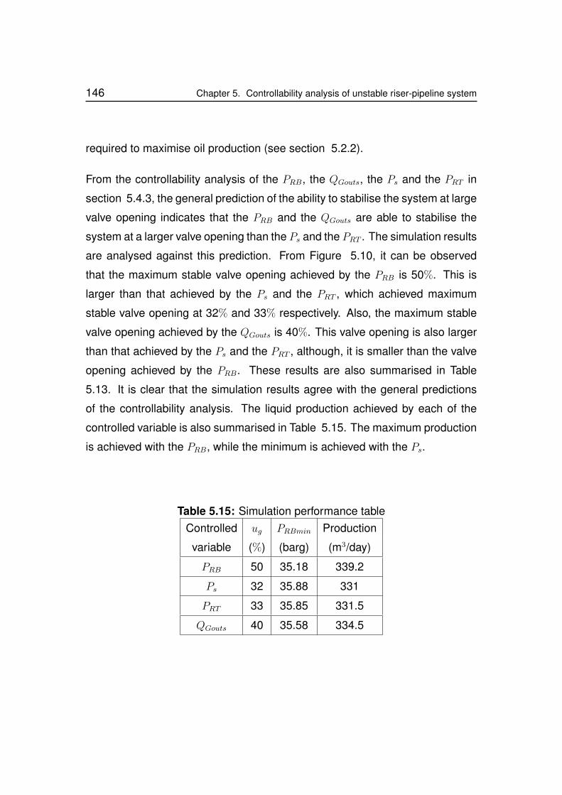
146 Chapter 5. Controllability analysis of unstable riser-pipeline system
required to maximise oil production (see section 5.2.2).
From the controllability analysis of the PRB, the QGouts, the Ps and the PRT in
section 5.4.3, the general prediction of the ability to stabilise the system at large
valve opening indicates that the PRB and the QGouts are able to stabilise the
system at a larger valve opening than the Ps and the PRT . The simulation results
are analysed against this prediction. From Figure 5.10, it can be observed
that the maximum stable valve opening achieved by the PRB is 50%. This is
larger than that achieved by the Ps and the PRT , which achieved maximum
stable valve opening at 32% and 33% respectively. Also, the maximum stable
valve opening achieved by the QGouts is 40%. This valve opening is also larger
than that achieved by the Ps and the PRT , although, it is smaller than the valve
opening achieved by the PRB. These results are also summarised in Table
5.13. It is clear that the simulation results agree with the general predictions
of the controllability analysis. The liquid production achieved by each of the
controlled variable is also summarised in Table 5.15. The maximum production
is achieved with the PRB, while the minimum is achieved with the Ps.
Table 5.15: Simulation performance tableControlled ug PRBmin Production
variable (%) (barg) (m3/day)
PRB 50 35.18 339.2
Ps 32 35.88 331
PRT 33 35.85 331.5
QGouts 40 35.58 334.5

Chapter 5. Controllability analysis of unstable riser-pipeline system 147
5.6 Comparison of the controllability with u and ug
In this section, a general comparison of the controllability of the industrial riser
system using the u and the ug is presented. Firstly, it can be observed that the
riser-pipeline system can be controlled by using either u or ug as the manipu-
lated variable. Generally, the controllability analysis showed that both u and ughave the ability to stabilise the system at large valve opening with the riser base
pressure and the gas volumetric flow rate as the controlled variables. For the
PRT , the controllability analysis showed its limited ability to stabilise the system
at a large valve opening for the two manipulated variables.
From the simulation result analysis, the control with ug showed the ability to
stabilise the system at a slightly higher valve opening than control with the u.
However, due to the differences in the individual valve characteristics in the
industrial riser system, it is observed that although the control with ug achieved
stability at a slightly higher valve opening, the control with u achieved lower PRB,
when compared to an equivalent valve opening with the ug. This is shown in
Table 5.16, which shows the maximum stable valve opening (ums), the PRBmin,
and the production obtained through simulation for the PRB and the PRT .
Table 5.16: Controllability with u and ug comparison table
ums (%) PRBmin (barg) Production
(m3/day)
Variable u ug u ug u ug
PRB 49 50 34.54 35.18 348 339.2
PRT 33 33 35.58 35.85 334.5 331.5
As will be discussed in Chapter 6 and 7, in order to maximise oil production it
148 Chapter 5. Controllability analysis of unstable riser-pipeline system
is necessary to operate the system such that the flowline pressure is reduced
under stable operating condition. Although it is desired to stabilise the system
at a large valve opening in order to maximise oil production, this controllability
analysis also reveals that when analysing the controllability of the riser-pipeline
system for different valves as the manipulated variable, the minimum PRB ob-
tained, which can be affected by the individual valve characteristics must be
evaluated. This has been achieved through simulation analysis. It is shown
that for the industrial riser system used in this work, closed-loop control with u
will give a lower PRB than with ug for the same value of the valve opening.
5.7 Conclusions
In this chapter, the controllability analysis of the unstable riser-pipeline system
for stability and production has been presented. The control objectives are
defined to reflect the core operational targets of the riser-pipeline production
system, which are the ability to ensure system stability and achieve maximum
oil production. The interdependency between a stable valve opening and the
accumulated production was explored as the fundamental basis for the control-
lability analysis. It is shown that, the larger the stable valve opening achieved
in the system, the higher the ability to maximise oil production.
The ability of a slug control system to achieve these desired control objectives
are evaluated with focus on the choice of the controlled variables, using two
manipulated variables, which include the riser top valve opening and the top-
side separator gas valve opening. The controllability analysis was focused on
applying the Hankel singular value analysis of the system linear model to eval-
Chapter 5. Controllability analysis of unstable riser-pipeline system 149
uate the minimum control input magnitude required to stabilise the system at
each open-loop unstable valve opening.
The controllability analysis of the industrial riser system using u as the ma-
nipulated variable showed that theoretically, all the three controlled variables
considered, namely: the PRB, the PRT and the QT , has the ability to stabilise
the system at some open-loop unstable operating points without input satura-
tion. Also, the controllability analysis of the same industrial riser system using
the ug as the manipulated variable, showed that all the four controlled variables
considered namely: the PRB, the Ps, the PRT and the QGesp, has the ability to
stabilise the system at some open-loop unstable operating point without input
saturation. Interestingly, this controllability analysis also revealed the varying
ability of each controlled variable to stabilise the system at a large valve open-
ing.
Generally, using u as the manipulated variable, it was observed that the PRB
and the QT are able to stabilise the system at a larger valve opening than the
PRT . Also, by using ug as the manipulated variable, it was observed that the
PRB and the QGouts are able to stabilise the system at a larger valve opening
than thePs and the PRT . These results are important as they reflect the pro-
duction that is achievable with each controlled variable, under stable operating
condition.
A more suitable slug control strategy in which the unstable riser-pipeline system
is stabilised at a reference valve opening using a derivative controller action is
implemented to perform closed-loop simulation for each controlled variable. In
this controlled strategy, perfect tracking of the controlled variable set point was
neglected in the system such that the controlled variable set point is set equal to
zero, and the derivative controller input is the measured value of the controlled
150 5. My Third Chapter
variable, which is not necessarily zero. The derivative controller parameters are
obtained using the Routh stability criterion.
The closed-loop simulations in OLGA confirmed the general predictions of this
controllability analysis. In the simulation using u as the manipulated variable,
it was observed that the PRB and the QT are able to stabilise the system at
a larger valve opening than the PRT , as was predicted. However, it was also
observed that the PRB achieved stability at a slightly larger valve opening than
the QT . Also, in the simulation using ug as the manipulated variable, it was
confirmed that the PRB and the QGouts are able to stabilise the system at a
larger valve opening than thePs and the PRT . Simulation results also showed
that accumulated production increased with the ability to stabilise the system at
a large valve opening. In the simulation with the u, the maximum accumulated
production was obtained with the PRB and the minimum with the PRT . Also, in
the simulation with the ug, the maximum accumulated production was obtained
with the PRB and the minimum with the Ps.
Interestingly, this controllability analyses has shown that most controlled vari-
ables including the PRT which was considered to be unsuitable for slug control,
and the QT which was considered to be suitable if it is used in the inner feed-
back loop in a cascade control, can be used for slug control if an appropriate
slug control strategy, such that presented in this chapter is implemented.
Chapter 6
Production potential of severe slug
control system
6.1 Introduction
The primary objective of a slug control system which is to eliminate slugging
and ensure stable system operation has guided the common approach to slug
control systems design and implementation. One of the proven solutions to
slug control is the choking of the riser top valve. Choking transforms the unsta-
ble flow in the riser to stable flow. However, due to the additional pressure drop
across the valve, it induces extra back pressure on the pipeline. Active feed-
back, feed forward and cascade control systems have been applied to dynamic
choking for slug control [23, 32, 42, 51, 71, 75, 76, 101, 99].
Although the implementation of a slug controller in the active choking solution
has shown its potential to successfully eliminate severe slugging with some
benefits, it can also adversely affect the overall production of the system if it is
implemented inappropriately. As a result of this, the emphasis on the perfor-
mance of slug control systems has recently shifted from just achieving a stable
151
152 Chapter 6. Production potential of severe slug control system
system condition to also maximizing production [76].
However, the method for analysing the potential of a slug control system to
maximise production and how this potential can be achieved have remained
unclear. Most slug control systems are implemented without proper systematic
assessment of its potential to maximise production in the system. In this work,
a systematic method based on the pressure bifurcation map of the riser system
is proposed to analyse the production and pressure loss relationship, and to
reveal the potential of a slug control system to maximise production.
It is shown that for an unstable riser-pipeline system with known inlet and out-
let boundary conditions, production loss or gain due to operation in stable or
unstable operating conditions could be predicted using a pressure dependent
dimensionless variable known as the Production Gain Index (PGI). The chapter
starts with the description of the pressure and production dependency followed
by production estimation using the PGI and finally a case study.
6.2 Pressure and production
The ultimate aim of stabilising severe slugging flow conditions is to achieve
smooth and productive operation. Therefore, a slug control system should not
only consider stability but also maximise oil production. For this purpose, it is
necessary to analyse the effect of pressure loss associated with choking on
the oil production. For simplicity, linear relations are assumed in the analysis
below. Firstly, the pressure and production relationship of a linear well will be
discussed.
Chapter 6. Production potential of severe slug control system 153
6.2.1 Linear well productivity
The relationship for determining oil production rate from a linear well can be
derived generally from Darcy’s law [49] as given in (6.1), where qw is the well
production rate, B is the production index, Pres is the reservoir pressure and
PWH is the well-head pressure. The production index, B, is a function of the
reservoir geometric factor and the formation volume factor, which are depen-
dent on the reservoir dynamic characteristics (see section 4.3.4.1). In this anal-
ysis, it is assumed that the reservoir dynamic characteristics and pressure do
not change significantly over a reasonable period. Thus, the production index,
B, and the Pres will be assumed as constants.
qw = B(Pres − PWH) (6.1)
The relationship in (6.1) shows that qw ∝ (Pres − PWH). Therefore, an increase
in the production rate can be achieved by reducing PWH , which depends on a
number of system related factors including the downstream separator pressure,
and pressure loss across the pipeline and the riser. Here, the PWH dependency
on the valve opening including the pressure loss across the valve, the riser and
the pipeline will be consider. For a specific valve opening, the system can either
be stable or unstable. This will be analysed correspondingly as follows.
For a stable operating condition, the PWH can be fairly constant, while for an
unstable system, PWH will oscillate significantly. For both conditions, the total
production over a certain period T , is given as follows,
JW =
∫ T
0
qwdt = B(Pres − PWH)T = J0 − Jp (6.2)
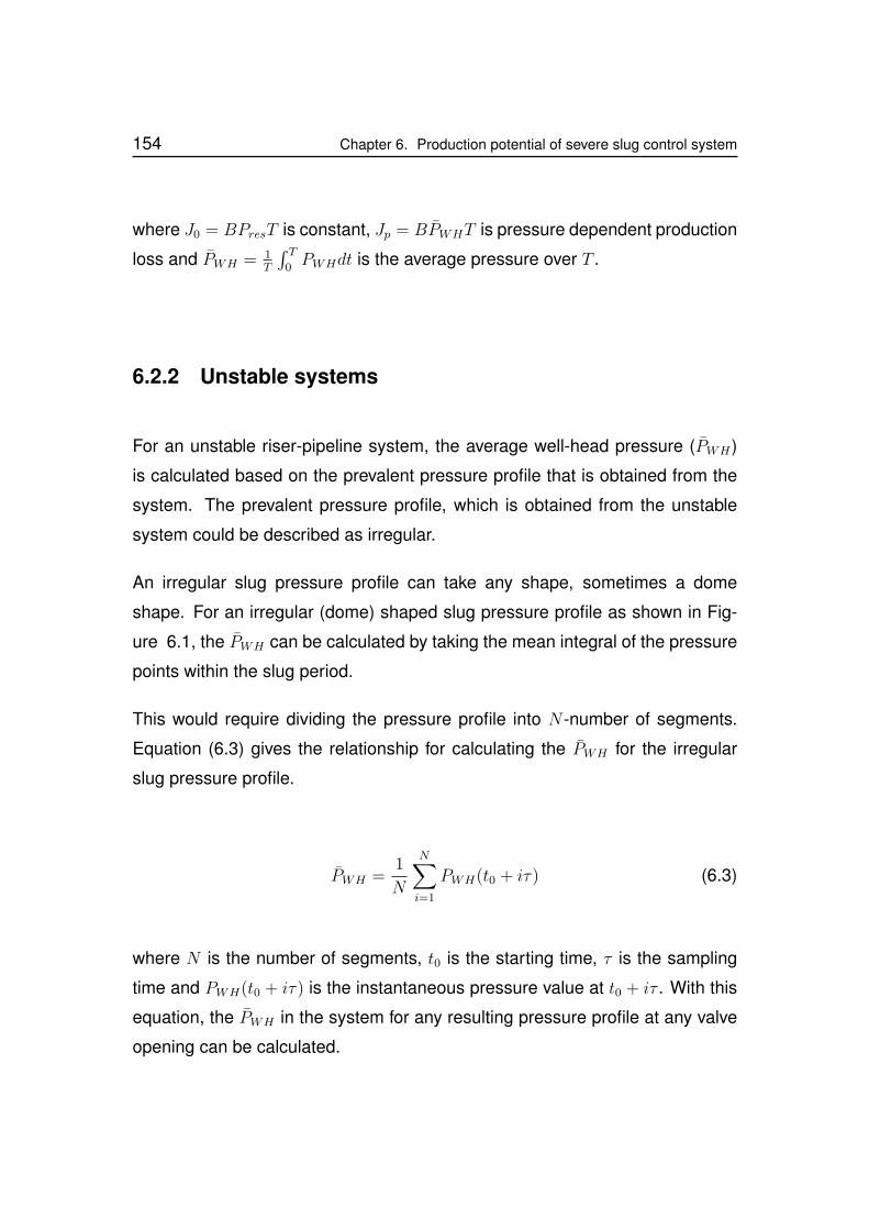
154 Chapter 6. Production potential of severe slug control system
where J0 = BPresT is constant, Jp = BPWHT is pressure dependent production
loss and PWH = 1T
∫ T0PWHdt is the average pressure over T .
6.2.2 Unstable systems
For an unstable riser-pipeline system, the average well-head pressure (PWH)
is calculated based on the prevalent pressure profile that is obtained from the
system. The prevalent pressure profile, which is obtained from the unstable
system could be described as irregular.
An irregular slug pressure profile can take any shape, sometimes a dome
shape. For an irregular (dome) shaped slug pressure profile as shown in Fig-
ure 6.1, the PWH can be calculated by taking the mean integral of the pressure
points within the slug period.
This would require dividing the pressure profile into N -number of segments.
Equation (6.3) gives the relationship for calculating the PWH for the irregular
slug pressure profile.
PWH =1
N
N∑i=1
PWH(t0 + iτ) (6.3)
where N is the number of segments, t0 is the starting time, τ is the sampling
time and PWH(t0 + iτ) is the instantaneous pressure value at t0 + iτ . With this
equation, the PWH in the system for any resulting pressure profile at any valve
opening can be calculated.
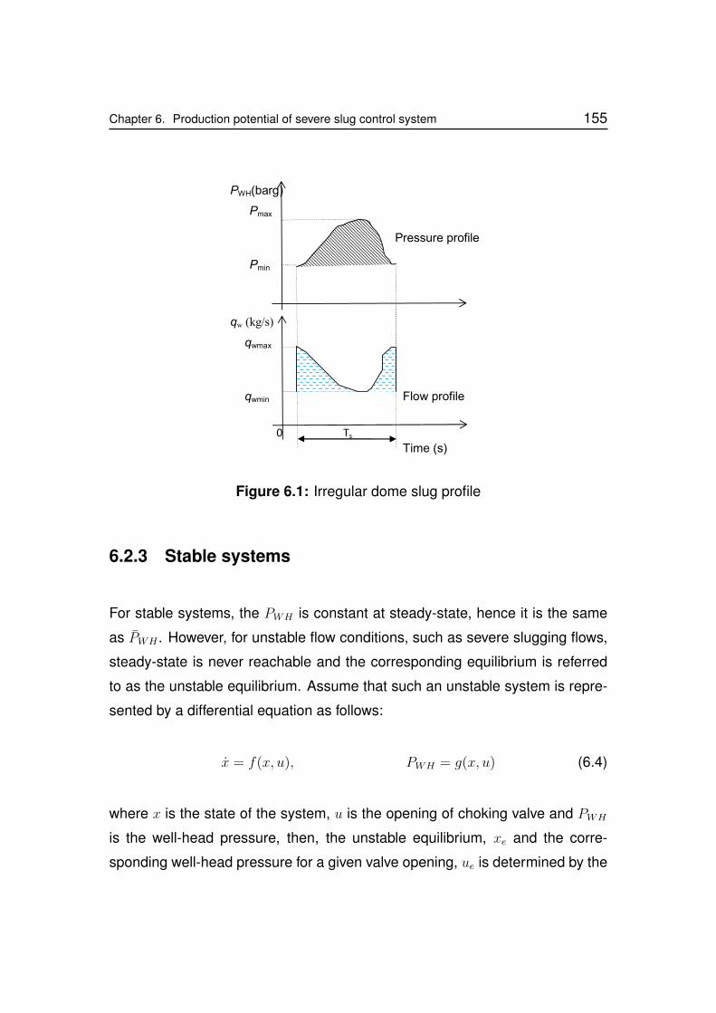
Chapter 6. Production potential of severe slug control system 155
qwmax
qwmin Flow profile
Time (s)
Pmax
Pressure profile
Pmin
PWH(barg)
qw (kg/s)
Ts0
Figure 6.1: Irregular dome slug profile
6.2.3 Stable systems
For stable systems, the PWH is constant at steady-state, hence it is the same
as PWH . However, for unstable flow conditions, such as severe slugging flows,
steady-state is never reachable and the corresponding equilibrium is referred
to as the unstable equilibrium. Assume that such an unstable system is repre-
sented by a differential equation as follows:
x = f(x, u), PWH = g(x, u) (6.4)
where x is the state of the system, u is the opening of choking valve and PWH
is the well-head pressure, then, the unstable equilibrium, xe and the corre-
sponding well-head pressure for a given valve opening, ue is determined by the
156 Chapter 6. Production potential of severe slug control system
algebraic equations, which are given in (6.5).
f(xe, ue) = 0, PWHe = g(xe, ue) (6.5)
If such an unstable system is stabilised by a feedback control, u = k(PWH),
then the steady-state of the stable closed-loop system, xc, PWHc and uc are
determined as follows.
0 = f(xc, uc), PWHc = g(xc, uc), uc = k(PWHc) (6.6)
Therefore, if ue = uc, then xe = xc and PWHe = PWHc, i.e. the steady-state of the
stable closed-loop system must be equal to the unstable equilibrium condition
in accordance with the same valve opening. The values of PWHc = PWHe at
the unstable equilibrium point corresponding to a particular valve opening can
be calculated using an accurate model of the system. However, it can also be
obtained using the multiphase flow simulator such as OLGA.
For the riser system, u is the valve opening, which determines the operating
point of the system. For a set of input values, say u = (u1, u2, ...un), the corre-
sponding equilibrium values x = (x1, x2, ...xn) are determined by (6.5). These
values can then be used for production analysis of active slug control.
6.3 Production Gain Index (PGI)
For a riser system stabilised by a slug controller operating at a valve position,
uc, the production gain when compared to an unstable slugging condition cor-
responding to an open-loop valve opening, u, is Jp(u) − Jp(uc). In order to
analyse the production potential of the slug control system, a dimensionless
variable, the Production Gain Index (PGI) is introduced as the ratio of the pro-
duction gain, Jp(u)− Jp(uc) against Jp(uc) as follows.
Chapter 6. Production potential of severe slug control system 157
ξ(u, uc) =Jp(u)− Jp(uc)
Jp(uc)=
PWH(u)
PWHc(uc)− 1 (6.7)
The PGI as a function of u and uc can be represented as contours in the (u, uc)
plane. Amongst these contours is the zero PGI (ZPGI) contour, which is defined
as ξ(u, uc) = 0. The ZPGI contour divides the (u, uc) plane into two areas,
namely: the positive PGI (PPGI) area, which is located above the ZPGI line
and the negative PGI (NPGI) area, which is located below the ZPGI line. A
typical example of this ZPGI contour is shown in Figure 6.4 for a case study,
which will be discussed in section 6.4.
According to the definition of the PGI in (6.7), the PPGI area corresponds to pro-
duction gain operating points, i.e. for any point (u, uc) in this area, if a slug con-
troller can stabilise the system at the valve opening, uc, then the corresponding
production will be larger than the one obtained when the valve opening is fixed
at u without any control. Similarly, the NPGI area indicates production loss op-
erating conditions, i.e. for a point (u, uc) in this area, if a slug control stabilises
the system with valve opening uc, the resulting production will be less than the
one corresponding to the valve opening fixed at u without control.
6.4 Case study - the industrial riser system
To illustrate the application of the PGI analysis method to reveal the produc-
tion potential of a riser-pipeline system, the industrial riser system, which is
described in section 3.5 will be used. The open-loop stability of this system
can be analysed using the Hopf bifurcation map presented in Figure 4.18. The
Hopf bifurcation map indicates that the maximum open-loop valve opening cor-
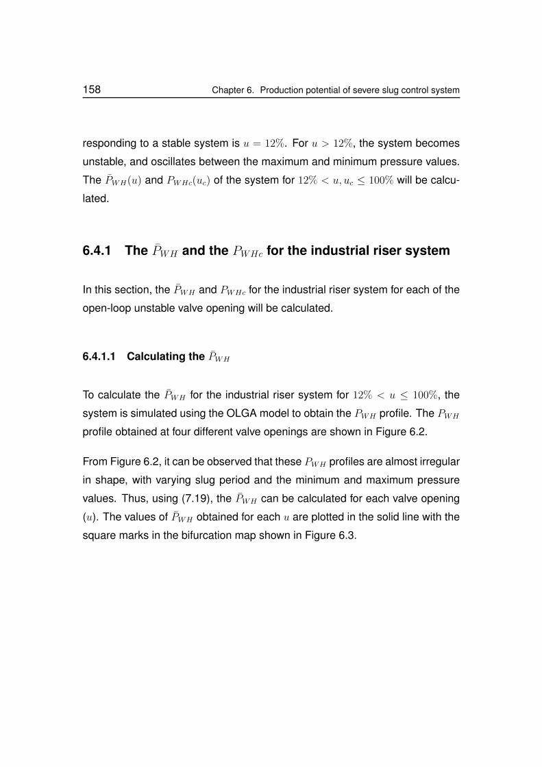
158 Chapter 6. Production potential of severe slug control system
responding to a stable system is u = 12%. For u > 12%, the system becomes
unstable, and oscillates between the maximum and minimum pressure values.
The PWH(u) and PWHc(uc) of the system for 12% < u, uc ≤ 100% will be calcu-
lated.
6.4.1 The PWH and the PWHc for the industrial riser system
In this section, the PWH and PWHc for the industrial riser system for each of the
open-loop unstable valve opening will be calculated.
6.4.1.1 Calculating the PWH
To calculate the PWH for the industrial riser system for 12% < u ≤ 100%, the
system is simulated using the OLGA model to obtain the PWH profile. The PWH
profile obtained at four different valve openings are shown in Figure 6.2.
From Figure 6.2, it can be observed that these PWH profiles are almost irregular
in shape, with varying slug period and the minimum and maximum pressure
values. Thus, using (7.19), the PWH can be calculated for each valve opening
(u). The values of PWH obtained for each u are plotted in the solid line with the
square marks in the bifurcation map shown in Figure 6.3.
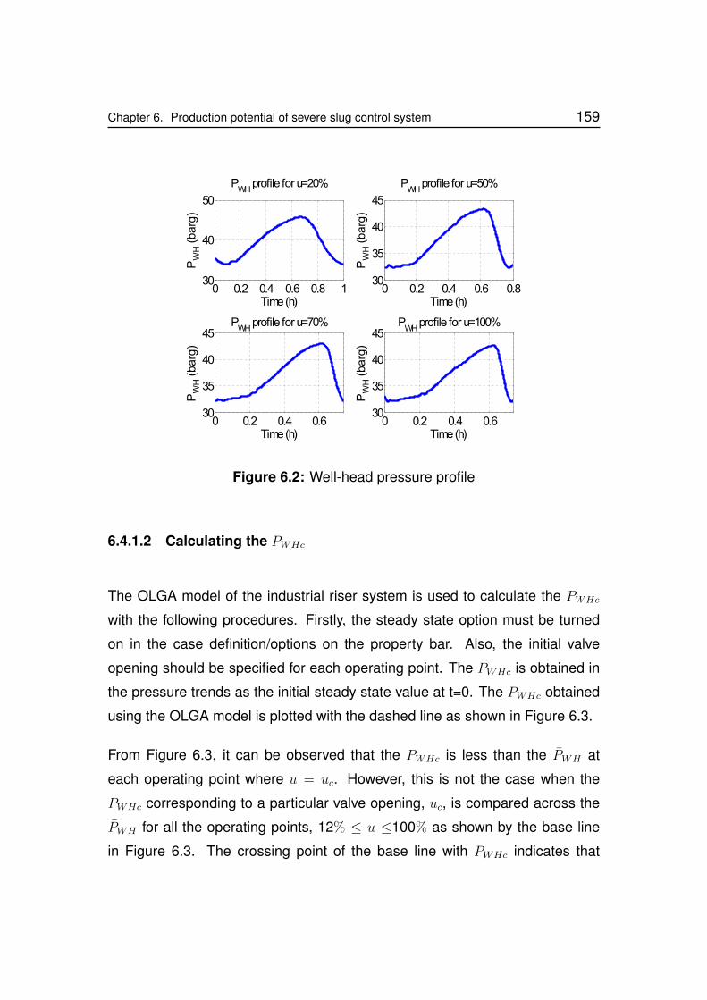
Chapter 6. Production potential of severe slug control system 159
0 0.2 0.4 0.6 0.8 130
40
50
PWH
profile for u=20%P
WH
(barg
)
Time(h)0 0.2 0.4 0.6 0.8
30
35
40
45
PWH
profile for u=50%
PW
H(b
arg
)
Time(h)
0 0.2 0.4 0.630
35
40
45P
WHprofile for u=70%
PW
H(b
arg
)
Time(h)0 0.2 0.4 0.6
30
35
40
45P
WHprofile for u=100%
PW
H(b
arg
)
Time(h)
Figure 6.2: Well-head pressure profile
6.4.1.2 Calculating the PWHc
The OLGA model of the industrial riser system is used to calculate the PWHc
with the following procedures. Firstly, the steady state option must be turned
on in the case definition/options on the property bar. Also, the initial valve
opening should be specified for each operating point. The PWHc is obtained in
the pressure trends as the initial steady state value at t=0. The PWHc obtained
using the OLGA model is plotted with the dashed line as shown in Figure 6.3.
From Figure 6.3, it can be observed that the PWHc is less than the PWH at
each operating point where u = uc. However, this is not the case when the
PWHc corresponding to a particular valve opening, uc, is compared across the
PWH for all the operating points, 12% ≤ u ≤100% as shown by the base line
in Figure 6.3. The crossing point of the base line with PWHc indicates that
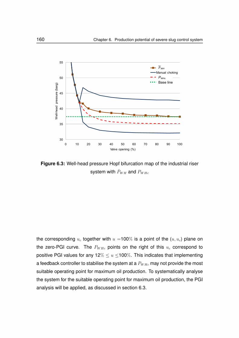
160 Chapter 6. Production potential of severe slug control system
30
35
40
45
50
55
0 10 20 30 40 50 60 70 80 90 100
We
ll-he
ad
pre
ssure
(ba
rg)
Valve opening (%)
Series3
Manual choking
Series4PWHc
WH
Base line
Figure 6.3: Well-head pressure Hopf bifurcation map of the industrial riser
system with PWH and PWHc
the corresponding uc together with u =100% is a point of the (u, uc) plane on
the zero-PGI curve. The PWHc points on the right of this uc correspond to
positive PGI values for any 12% ≤ u ≤100%. This indicates that implementing
a feedback controller to stabilise the system at a PWHc may not provide the most
suitable operating point for maximum oil production. To systematically analyse
the system for the suitable operating point for maximum oil production, the PGI
analysis will be applied, as discussed in section 6.3.
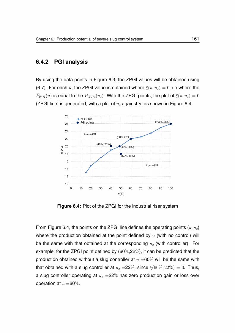
Chapter 6. Production potential of severe slug control system 161
6.4.2 PGI analysis
By using the data points in Figure 6.3, the ZPGI values will be obtained using
(6.7). For each u, the ZPGI value is obtained where ξ(u, uc) = 0, i.e where the
PWH(u) is equal to the PWHc(uc). With the ZPGI points, the plot of ξ(u, uc) = 0
(ZPGI line) is generated, with a plot of uc against u, as shown in Figure 6.4.
10
12
14
16
18
20
22
24
26
28
0 10 20 30 40 50 60 70 80 90 100
uc(%
)
u(%)
ZPGI linePGI points
(40%, 20%)
(50%,18%)
(60%,22%)
(100%,26%)
(49%,20%)
ξ(u, uc)>0
ξ(u, uc)<0
Figure 6.4: Plot of the ZPGI for the industrial riser system
From Figure 6.4, the points on the ZPGI line defines the operating points (u, uc)
where the production obtained at the point defined by u (with no control) will
be the same with that obtained at the corresponding uc (with controller). For
example, for the ZPGI point defined by (60%,22%), it can be predicted that the
production obtained without a slug controller at u =60% will be the same with
that obtained with a slug controller at uc =22%, since ξ(60%, 22%) = 0. Thus,
a slug controller operating at uc =22% has zero production gain or loss over
operation at u =60%.
162 Chapter 6. Production potential of severe slug control system
For any operating point on the ZPGI line defined by (u, uc), a PPGI will be
obtained with reference to the uc, for all open-loop valve openings less than
the corresponding u. From the reference uc, the open loop valve openings
less than the corresponding u will be traced above the ZPGI line. Thus, any
operating point defined by (u, uc) above the ZPGI line, corresponds to a PPGI
point, where the ξ(u, uc) > 0. The production obtained with a slug controller,
which stabilises the system at uc, will be higher than that obtained with the
system operating at u without control.
For example, for the PPGI point defined by (40%,20%) in Figure 6.4, it can
be predicted that the production obtained with a slug controller at uc =20%
will be higher than that obtained without a slug controller at u =40%, since
ξ(40%, 20%) > 0. Also, for the ZPGI point defined by (49%, 20%), it can be
predicted that the production obtained with a slug controller at uc =20% will be
higher than that obtained for all open-loop valve openings u <49%.
Furthermore, for any point on the ZPGI line defined by (u, uc), a NPGI will be
obtained with reference to the uc for all open-loop valve openings larger than
the corresponding u. From the reference uc, the open loop valve openings
larger than the corresponding u will be traced below the ZPGI line. Thus, any
operating point defined by (u, uc) below the ZPGI line corresponds to a NPGI
point, where the ξ(u, uc) < 0. This implies that the production obtained with a
slug controller, which stabilises the system at uc, will be less than that obtained
with the system operating at u without control.
For example, for the NPGI point defined by (50%,18%) in Figure 6.3, it can be
predicted that the production obtained with a slug controller at uc =18% will be
less than that obtained without a slug controller at u =50%, since ξ(50%, 18%) <
0. Thus, for the ZPGI point defined by (49%,20%), it can be predicted that the
Chapter 6. Production potential of severe slug control system 163
production obtained with a slug controller at uc = 20% will be less than that
obtained for all open-loop operating points u >49%. From these analyses, it can
also be deduced that for the ZPGI point defined by (100%,26%), the production
obtained with a slug controller at uc >26% will be higher than that obtained for
all open-loop valve openings u ≤100%.
These analyses provide a very useful insight into the production potential of
this industrial riser system, using a slug controller. The PGI analysis reveals
that the extent to which a feedback controller can assure increased production
depends on the maximum closed-loop operating point the feedback controller
can achieve. Since the ZPGI line is independent of the control design but de-
pendent on the riser-pipeline system design, the operating condition and the
flow condition, the decision on whether to implement a feedback controller or
not in order to stabilise the riser system as well as maximise production can
easily be made without rigorous simulations or costly trial and error method.
6.4.3 Simulated production
In this section, the actual production obtained from a 24 hour simulation of the
industrial riser system under closed-loop and open-loop operating condition will
be analysed and compared with the predictions of the PGI analysis.
6.4.3.1 The simulation model and controller
Open-loop simulation is performed for several operating points in the range
of 15% ≤ u ≤ 100% and the accumulated production for a 24 hour period
is recorded. Unlike the open-loop simulation, the closed-loop simulation will

164 Chapter 6. Production potential of severe slug control system
require a stabilising controller. To meet this requirement, two slug controllers
namely:
1. relay tuned slug controller
2. robust PID slug controller
are implemented and analysed. The design of the relay tuned slug controller
and the robust PID slug controller will be discussed in details in Chapter 7.
Both the open-loop and closed-loop simulations are carried out on the nonlin-
ear model of the industrial riser system in OLGA. The closed-loop simulation
is carried out using the OLGA-Matlab link, which is established by using the
OLGA-Matlab toolbox (see section 5.5.1).
6.4.3.2 Implementation of the relay tuned slug controller
The implemented relay tuned slug controller (K1) is a PI controller. The relay is
designed using process parameters obtained from the system response which
is determined by the shape factor analysis. The controller transfer function is
given in (6.8).
K1 =−4.02s− 0.18
22.4s(6.8)
This controller when implemented on the industrial riser system can stabilise
the system to a maximum closed-loop operating point of uc =28.3%. The open
and closed-loop simulated productions are shown in Figure 6.5
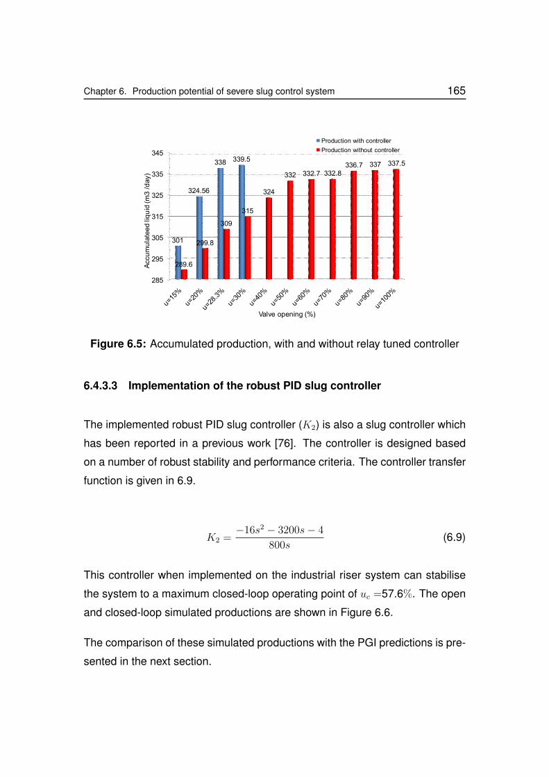
Chapter 6. Production potential of severe slug control system 165
285
295
305
315
325
335
345
301
324.56
338 339.5
289.6
299.8
309
315
324
332 332.7 332.8336.7 337 337.5
Accu
mu
late
ed
liqu
id(m
3/d
ay)
Valve opening (%)
Production with controller
Production without controller
Figure 6.5: Accumulated production, with and without relay tuned controller
6.4.3.3 Implementation of the robust PID slug controller
The implemented robust PID slug controller (K2) is also a slug controller which
has been reported in a previous work [76]. The controller is designed based
on a number of robust stability and performance criteria. The controller transfer
function is given in 6.9.
K2 =−16s2 − 3200s− 4
800s(6.9)
This controller when implemented on the industrial riser system can stabilise
the system to a maximum closed-loop operating point of uc =57.6%. The open
and closed-loop simulated productions are shown in Figure 6.6.
The comparison of these simulated productions with the PGI predictions is pre-
sented in the next section.

166 Chapter 6. Production potential of severe slug control system
285
295
305
315
325
335
345
355
301
324.56
339.5
289.6
299.8
Acc
um
ula
ted
liquid
(m3
/day
)
339.5
345348.12 348.17
315
324
332 332.5 332.7 332.8
Valve opening (%)
Production with controllerProduction without controller
332.8336.7 337 337.5
Production with controllerProduction without controller
Figure 6.6: Accumulated production, with and without robust PID controller
6.4.4 Simulated production comparison
From the simulated production obtained using the two slug controllers, it is
observed that the production at uc =20% is 3% and 0.17% higher than the
open-loop production at u =30% and u =40% respectively. However, the open-
loop production at u=50% is 2.29% higher than the closed-loop production at
uc =20%.
Comparing these productions to the PGI predictions in section 6.4.2, which pre-
dicted that closed-loop production at uc =20% will be higher than the open-loop
production at any operating point of u <49%, and that closed-loop production
at uc =20% will be less than the open-loop production at any operating point of
u >49%, it can be observed that the simulated production at uc =20% agrees
with the PGI predictions. When similar comparison is done for the closed-loop
production at u =15%, the simulated production also agrees with the prediction
of the PGI analysis.
Chapter 6. Production potential of severe slug control system 167
Also, it can be observed from the simulated production that the closed-loop
production at uc ≥30% is higher than the open-loop production for all the open-
loop operating points, 15% ≤ u ≤ 100%. Thus, the production of the relay
tuned slug controller at uc =28.3% is higher than the production at all the open-
loop operating points, 15% ≤ u ≤ 100%. This is also the case for the robust
PID controller at uc =57.6%. This agrees with the PGI prediction defined by the
point (100%,26%) in Figure 6.4.
Thus, the above analysis confirms that the production potentials of the riser-
pipeline system predicted by the PGI analysis agrees with all the actual sim-
ulated production results. Hence, at this point, it is clear that with proper PGI
analysis of a riser-pipeline system, the production potential of the system at
any operating point can be predicted.
6.4.5 PGI analysis for different reservoir pressures
With the industrial riser system, the PGI analysis can be performed for different
reservoir pressures. This analysis can reveal the potential of the slug control
system to maximise oil production for a declining reservoir pressure. To perform
this analysis, the ZPGI line is plotted for three reservoir pressures namely: 79
barg, 69 barg and 59 barg. The obtained ZPGI line plots are shown in Figure
6.7.
From this Figure 6.7, it can be observed that for a given u, the corresponding uc,
which defines the ZPGI point decreases as the reservoir pressure decreases.
Thus, the ZPGI line of a reservoir with lower pressure is located within the NPGI
region of a reservoir with higher pressure. For example, the ZPGI line of the
59 barg reservoir is located below the ZPGI line of the 69 barg reservoir. Thus,
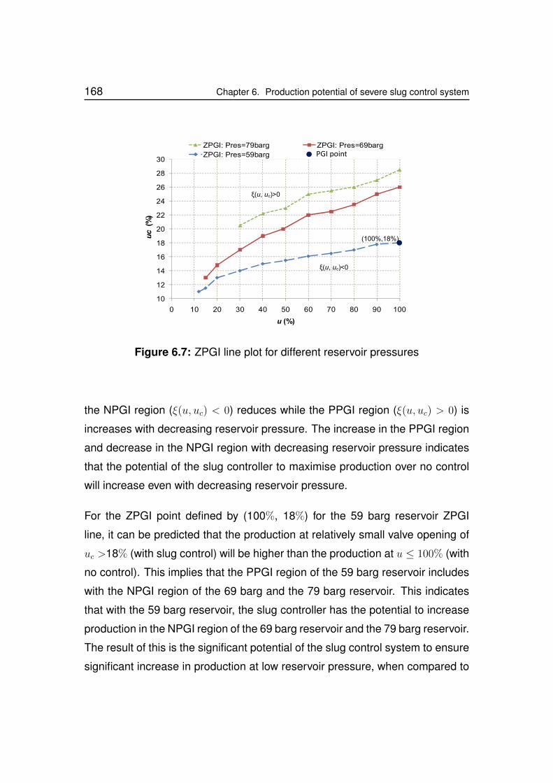
168 Chapter 6. Production potential of severe slug control system
10
12
14
16
18
20
22
24
26
28
30
0 10 20 30 40 50 60 70 80 90 100
uc
(%)
u (%)
ZPGI: Pres=79barg ZPGI: Pres=69barg
ZPGI: Pres=59barg
(100%,18%)
ξ(u, uc)>0
ξ(u, uc)<0
PGI point
Figure 6.7: ZPGI line plot for different reservoir pressures
the NPGI region (ξ(u, uc) < 0) reduces while the PPGI region (ξ(u, uc) > 0) is
increases with decreasing reservoir pressure. The increase in the PPGI region
and decrease in the NPGI region with decreasing reservoir pressure indicates
that the potential of the slug controller to maximise production over no control
will increase even with decreasing reservoir pressure.
For the ZPGI point defined by (100%, 18%) for the 59 barg reservoir ZPGI
line, it can be predicted that the production at relatively small valve opening of
uc >18% (with slug control) will be higher than the production at u ≤ 100% (with
no control). This implies that the PPGI region of the 59 barg reservoir includes
with the NPGI region of the 69 barg and the 79 barg reservoir. This indicates
that with the 59 barg reservoir, the slug controller has the potential to increase
production in the NPGI region of the 69 barg reservoir and the 79 barg reservoir.
The result of this is the significant potential of the slug control system to ensure
significant increase in production at low reservoir pressure, when compared to
Chapter 6. Production potential of severe slug control system 169
no control production. This has the potential to extend the operation life of the
oil field. This potential will be discussed in details with simulation results in
section 7.5.2, where the stability and production in declining reservoir pressure
condition is discussed.
6.5 Conclusions
In conclusion, this chapter has presented a new concept known as the PGI
analysis, for accurately predicting the production potential of the unstable riser-
pipeline system. The PGI analysis reveals the potential of gaining or loosing
production due to the system’s operating point and operating condition. The
application of the PGI analysis employs a systematic analysis of the pressure
and production relationship in a riser-pipeline system, using a bifurcation map.
By using the PGI analysis, suitable operating point(s) for maximising production
with or without a slug controller can be predicted. The ZPGI contours which
is defined as ξ(u, uc) = 0, divides the (u, uc) plane into two areas namely: the
positive PGI (PPGI) area, which is located above the ZPGI line and the negative
PGI (NPGI) area, which is located below the ZPGI line. Operating point on the
ZPGI line defined by (u, uc) indicates the operating point where the production
with a slug controller at uc will be equal to production without a slug controller
(unstable system) at u. Any operating point, (u, uc), located above the ZPGI
line corresponds to production gain operating point known as the PPGI, while
any operating point located below the ZPGI line corresponds to a production
loss operating point, known as the NPGI.
170 Chapter 6. Production potential of severe slug control system
In order to achieve production gain at the predicted operating point, the de-
signed slug controller must be able to stabilise the system at the predicted
operating point. If the slug controller cannot achieve stability at the predicted
operating point, then the potential to achieve production gain is undermined.
The implementation of the PGI analysis on the industrial riser system shows
that the prediction of the PGI analysis agrees with the actual simulated produc-
tion. The ZPGI line plot for different reservoir pressures shows that the NPGI
region decreases, while the PPGI region increases with decreasing reservoir
pressure. This showed that the potential of the slug controller to maximise pro-
duction will increase even with decreasing reservoir pressure. These results
are very significant when planning control strategy for stability and production,
especially for brown fields.
Chapter 7
Design and characterisation of
slug controllers for maximising oil
production
7.1 Introduction
The primary objective of a slug control system is to stabilise the riser-pipeline
system by suppressing severe slugging. In addition to the requirement for a
slug control system to achieve stability, the emphasis on the system produc-
tivity has become of interest. The interest on the performance of slug control
systems has recently shifted from just achieving a stable operating condition to
also maximising production [76].
In Chapter 6, the systematic method for determining the production potential
of slug control of an unstable riser-pipeline system, using the production gain
index (PGI) was presented. It was explained that by using the production gain
index (PGI), the closed-loop valve opening where maximum oil production can
be achieved can be predicted. Once this suitable closed-loop valve opening
171
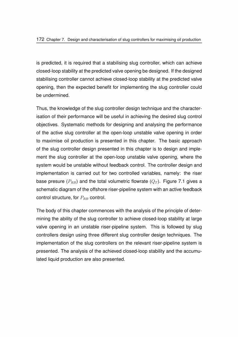
172 Chapter 7. Design and characterisation of slug controllers for maximising oil production
is predicted, it is required that a stabilising slug controller, which can achieve
closed-loop stability at the predicted valve opening be designed. If the designed
stabilising controller cannot achieve closed-loop stability at the predicted valve
opening, then the expected benefit for implementing the slug controller could
be undermined.
Thus, the knowledge of the slug controller design technique and the character-
isation of their performance will be useful in achieving the desired slug control
objectives. Systematic methods for designing and analysing the performance
of the active slug controller at the open-loop unstable valve opening in order
to maximise oil production is presented in this chapter. The basic approach
of the slug controller design presented in this chapter is to design and imple-
ment the slug controller at the open-loop unstable valve opening, where the
system would be unstable without feedback control. The controller design and
implementation is carried out for two controlled variables, namely: the riser
base presure (PRB) and the total volumetric flowrate (QT ). Figure 7.1 gives a
schematic diagram of the offshore riser-pipeline system with an active feedback
control structure, for PRB control.
The body of this chapter commences with the analysis of the principle of deter-
mining the ability of the slug controller to achieve closed-loop stability at large
valve opening in an unstable riser-pipeline system. This is followed by slug
controllers design using three different slug controller design techniques. The
implementation of the slug controllers on the relevant riser-pipeline system is
presented. The analysis of the achieved closed-loop stability and the accumu-
lated liquid production are also presented.
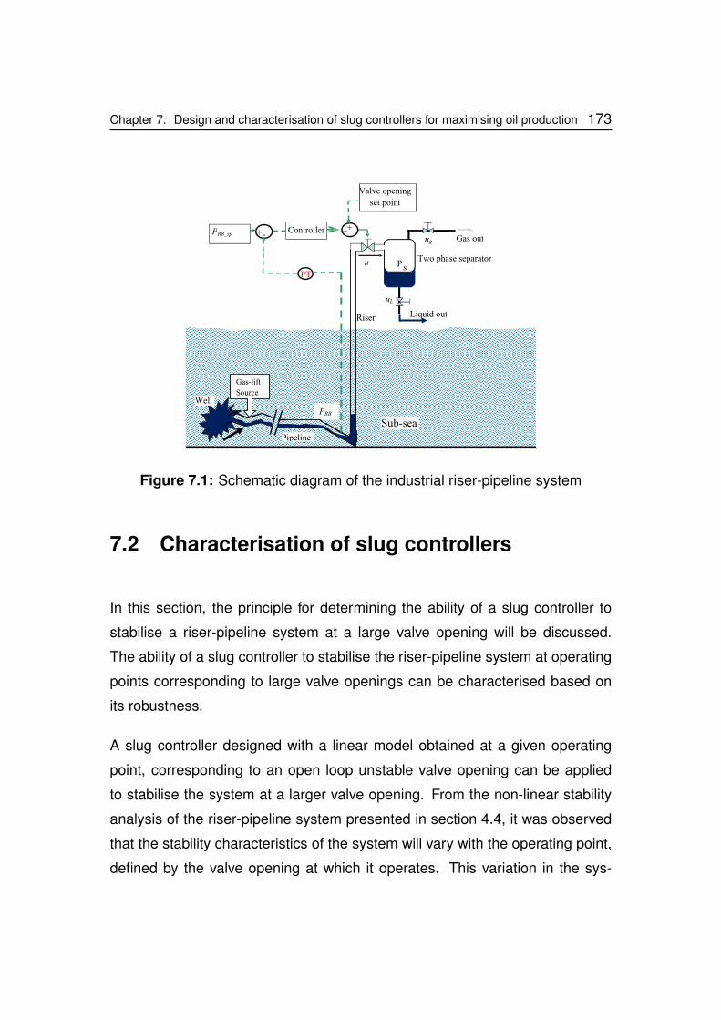
Chapter 7. Design and characterisation of slug controllers for maximising oil production 173
PRB
Valve opening
set point
ug
PsTwo phase separator
PT
+ Controller-
u
PRB_sp ++
Riser Liquid out
Gas out
Well
Pipeline
Gas-lift
Source
uL
Sub-sea
Figure 7.1: Schematic diagram of the industrial riser-pipeline system
7.2 Characterisation of slug controllers
In this section, the principle for determining the ability of a slug controller to
stabilise a riser-pipeline system at a large valve opening will be discussed.
The ability of a slug controller to stabilise the riser-pipeline system at operating
points corresponding to large valve openings can be characterised based on
its robustness.
A slug controller designed with a linear model obtained at a given operating
point, corresponding to an open loop unstable valve opening can be applied
to stabilise the system at a larger valve opening. From the non-linear stability
analysis of the riser-pipeline system presented in section 4.4, it was observed
that the stability characteristics of the system will vary with the operating point,
defined by the valve opening at which it operates. This variation in the sys-
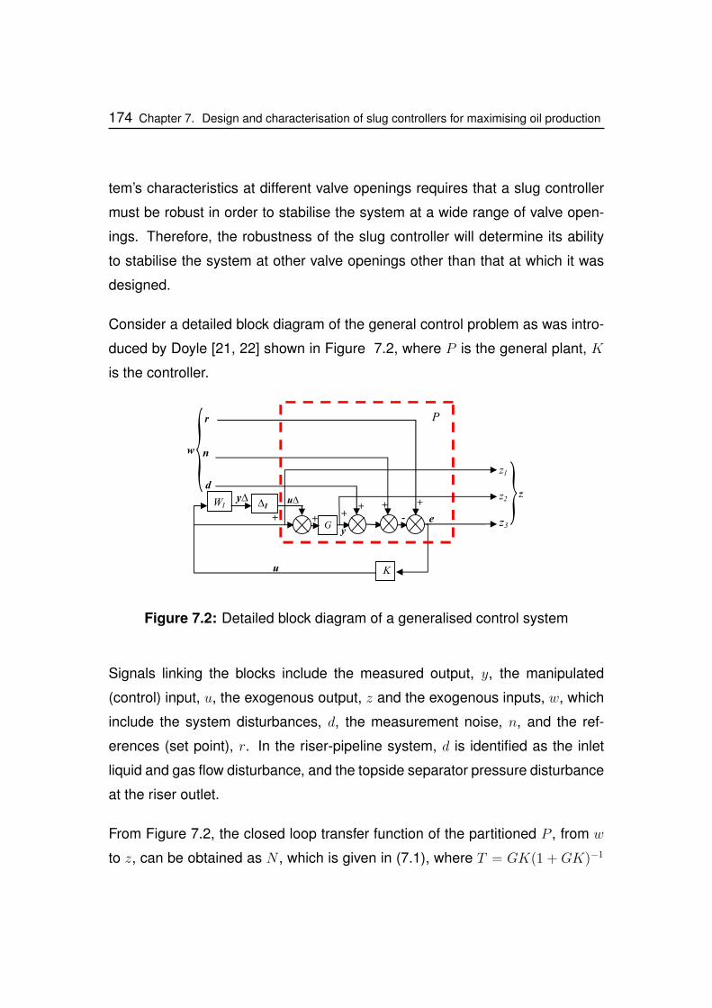
174 Chapter 7. Design and characterisation of slug controllers for maximising oil production
tem’s characteristics at different valve openings requires that a slug controller
must be robust in order to stabilise the system at a wide range of valve open-
ings. Therefore, the robustness of the slug controller will determine its ability
to stabilise the system at other valve openings other than that at which it was
designed.
Consider a detailed block diagram of the general control problem as was intro-
duced by Doyle [21, 22] shown in Figure 7.2, where P is the general plant, K
is the controller.
ze
∆Iy∆
u
z1
z2
z3
K
WI
G
r
n
d
w
+
-+
+++
y
P
u∆
+
Figure 7.2: Detailed block diagram of a generalised control system
Signals linking the blocks include the measured output, y, the manipulated
(control) input, u, the exogenous output, z and the exogenous inputs, w, which
include the system disturbances, d, the measurement noise, n, and the ref-
erences (set point), r. In the riser-pipeline system, d is identified as the inlet
liquid and gas flow disturbance, and the topside separator pressure disturbance
at the riser outlet.
From Figure 7.2, the closed loop transfer function of the partitioned P , from w
to z, can be obtained as N , which is given in (7.1), where T = GK(1 + GK)−1
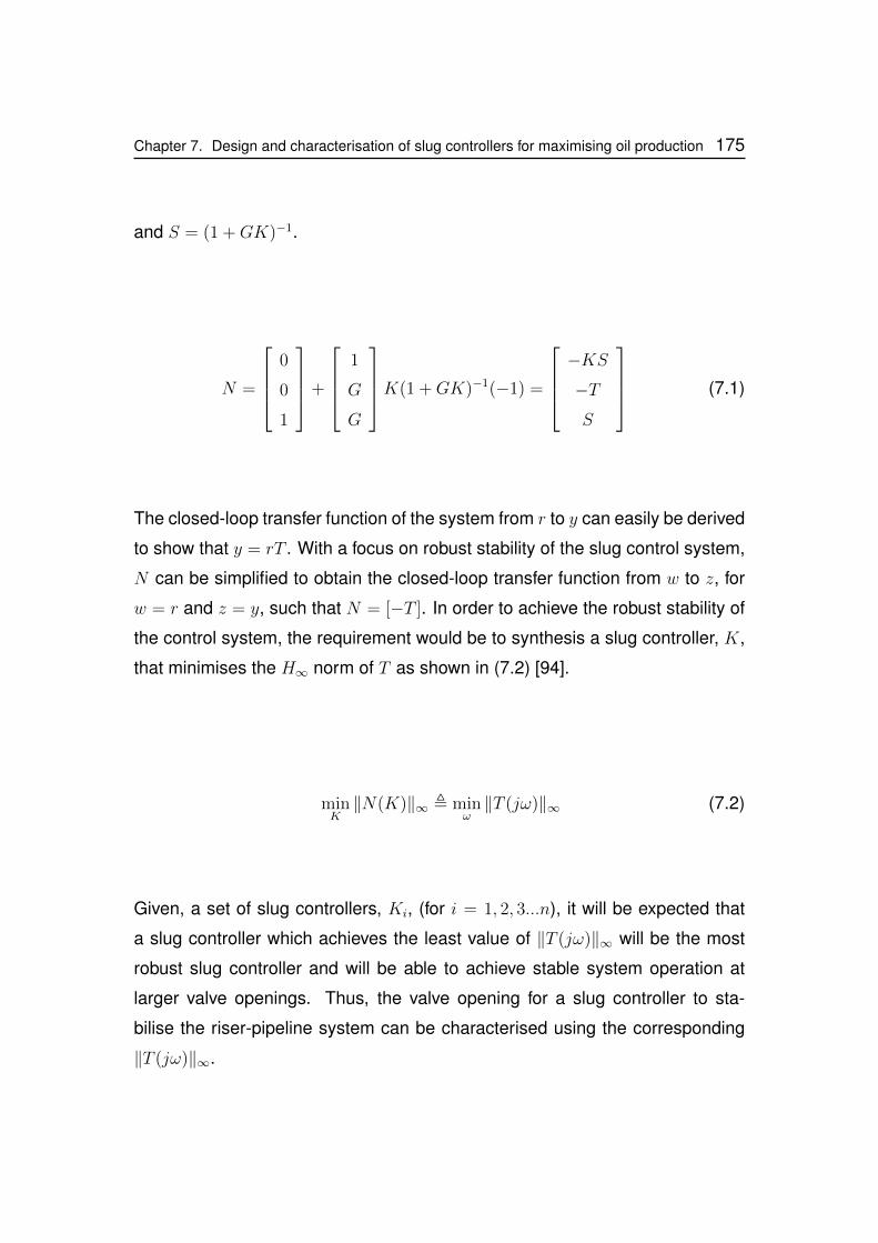
Chapter 7. Design and characterisation of slug controllers for maximising oil production 175
and S = (1 +GK)−1.
N =
0
0
1
+
1
G
G
K(1 +GK)−1(−1) =
−KS−TS
(7.1)
The closed-loop transfer function of the system from r to y can easily be derived
to show that y = rT . With a focus on robust stability of the slug control system,
N can be simplified to obtain the closed-loop transfer function from w to z, for
w = r and z = y, such that N = [−T ]. In order to achieve the robust stability of
the control system, the requirement would be to synthesis a slug controller, K,
that minimises the H∞ norm of T as shown in (7.2) [94].
minK‖N(K)‖∞ , min
ω‖T (jω)‖∞ (7.2)
Given, a set of slug controllers, Ki, (for i = 1, 2, 3...n), it will be expected that
a slug controller which achieves the least value of ‖T (jω)‖∞ will be the most
robust slug controller and will be able to achieve stable system operation at
larger valve openings. Thus, the valve opening for a slug controller to sta-
bilise the riser-pipeline system can be characterised using the corresponding
‖T (jω)‖∞.
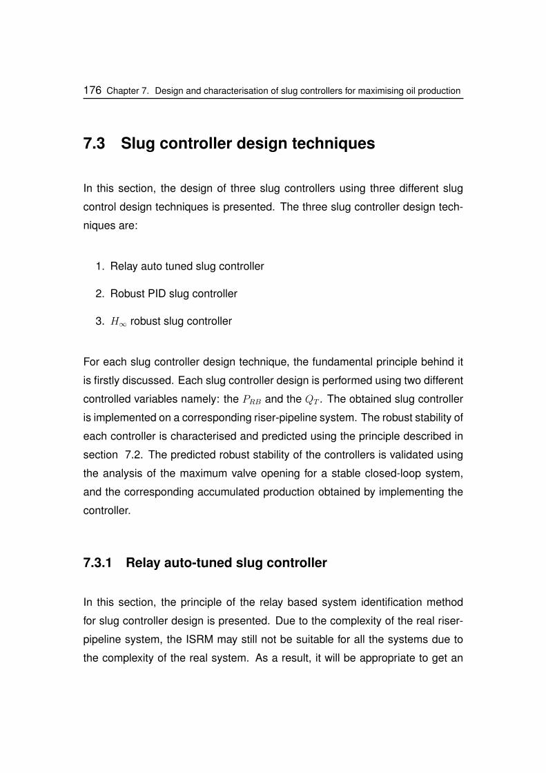
176 Chapter 7. Design and characterisation of slug controllers for maximising oil production
7.3 Slug controller design techniques
In this section, the design of three slug controllers using three different slug
control design techniques is presented. The three slug controller design tech-
niques are:
1. Relay auto tuned slug controller
2. Robust PID slug controller
3. H∞ robust slug controller
For each slug controller design technique, the fundamental principle behind it
is firstly discussed. Each slug controller design is performed using two different
controlled variables namely: the PRB and the QT . The obtained slug controller
is implemented on a corresponding riser-pipeline system. The robust stability of
each controller is characterised and predicted using the principle described in
section 7.2. The predicted robust stability of the controllers is validated using
the analysis of the maximum valve opening for a stable closed-loop system,
and the corresponding accumulated production obtained by implementing the
controller.
7.3.1 Relay auto-tuned slug controller
In this section, the principle of the relay based system identification method
for slug controller design is presented. Due to the complexity of the real riser-
pipeline system, the ISRM may still not be suitable for all the systems due to
the complexity of the real system. As a result, it will be appropriate to get an
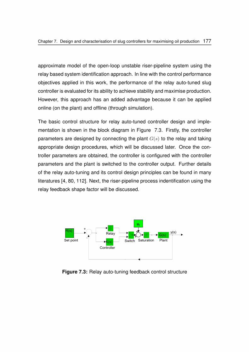
Chapter 7. Design and characterisation of slug controllers for maximising oil production 177
approximate model of the open-loop unstable riser-pipeline system using the
relay based system identification approach. In line with the control performance
objectives applied in this work, the performance of the relay auto-tuned slug
controller is evaluated for its ability to achieve stability and maximise production.
However, this approach has an added advantage because it can be applied
online (on the plant) and offline (through simulation).
The basic control structure for relay auto-tuned controller design and imple-
mentation is shown in the block diagram in Figure 7.3. Firstly, the controller
parameters are designed by connecting the plant G(s) to the relay and taking
appropriate design procedures, which will be discussed later. Once the con-
troller parameters are obtained, the controller is configured with the controller
parameters and the plant is switched to the controller output. Further details
of the relay auto-tuning and its control design principles can be found in many
literatures [4, 80, 112]. Next, the riser-pipeline process indentification using the
relay feedback shape factor will be discussed.
Saturation
Relay G(s)
Plant
R(s)
Set point K(s)
Controller
Switch
y(s)+
-
+
ur
+
Figure 7.3: Relay auto-tuning feedback control structure
178 Chapter 7. Design and characterisation of slug controllers for maximising oil production
7.3.1.1 Process identification using relay feedback shape factor
The first step in the relay auto-tuned controller design for the riser-pipeline sys-
tem is to identify the riser-pipeline process model by approximation, using the
relay feedback shape factor. To achieve this, the riser-pipeline system, G(s), is
first connected to the relay. The system is configured by defining a reference
valve opening, ur, which corresponds to an open-loop unstable condition. Also,
the controlled variable set point is defined at a suitable operating point, which
corresponds to the unstable equilibrium point in the open-loop unstable region.
The relay is then configured by defining the switch on and off point (a), which
is specified around the output variable set point, and defining the relay height,
h (relay output when on and off), which is specified around the reference valve
opening.
y(s)
Pu
u
h
a
D
time (s)
time (s)
Figure 7.4: Relay test feedback response
Chapter 7. Design and characterisation of slug controllers for maximising oil production 179
Having configured the relay, the required relay feedback response is obtained
by running the system. At first, the system input, u, is increased by +h and the
output y(s) decreases, (for PRB control). As the output decreases below the
switch off point (a), the input decreases by −h, such that the output increases
again. This results to a limit cycle feedback response, known as the relay
feedback response, with period, Pu, which is known as the ultimate period. The
shape of the resulting relay feedback response, which is used to approximate
and identify the process type can vary, depending on the ratio of the dead time
D to the process time constant τ [112].
In this application, the riser-pipeline process is identified as a first-order-plus-
dead-time (FOPDT) process. In order to identify this process, the feedback
response of the riser-pipeline system must satisfy certain characteristics based
on the shape of the response. These characteristics as reported by Thyagara-
jan and Yu [112] states that an unstable system whose relay feedback response
has sharp edges at the peak amplitude with a sustained oscillation can be ap-
proximated by a first-order-plus-dead-time (FOPDT) system. Figure 7.4 shows
a schematic diagram of the nature of this response. Three important parame-
ters D, a and Pu are obtained from the relay feedback response, where D is the
dead time, a is the peak amplitude and Pu is the ultimate period.
An unstable FOPDT system is defined by the process transfer function given
in (7.3), where τ is the time constant, kP is the process gain. The model pa-
rameters obtained from the relay feedback response are used to calculate the
parameters of the process transfer function.
G(s) =kpe−Ds
τs− 1(7.3)
A stabilising slug controller can be designed based on the identified process
parameters.
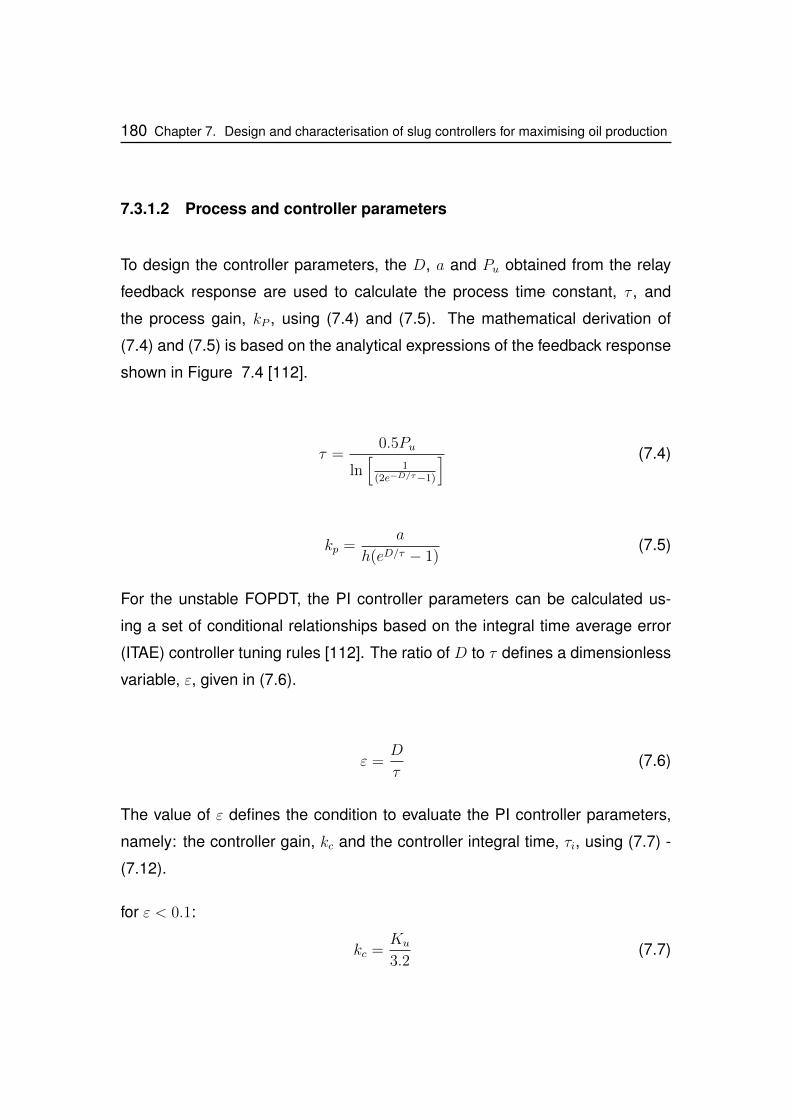
180 Chapter 7. Design and characterisation of slug controllers for maximising oil production
7.3.1.2 Process and controller parameters
To design the controller parameters, the D, a and Pu obtained from the relay
feedback response are used to calculate the process time constant, τ , and
the process gain, kP , using (7.4) and (7.5). The mathematical derivation of
(7.4) and (7.5) is based on the analytical expressions of the feedback response
shown in Figure 7.4 [112].
τ =0.5Pu
ln[
1(2e−D/τ−1)
] (7.4)
kp =a
h(eD/τ − 1)(7.5)
For the unstable FOPDT, the PI controller parameters can be calculated us-
ing a set of conditional relationships based on the integral time average error
(ITAE) controller tuning rules [112]. The ratio of D to τ defines a dimensionless
variable, ε, given in (7.6).
ε =D
τ(7.6)
The value of ε defines the condition to evaluate the PI controller parameters,
namely: the controller gain, kc and the controller integral time, τi, using (7.7) -
(7.12).
for ε < 0.1:
kc =Ku
3.2(7.7)
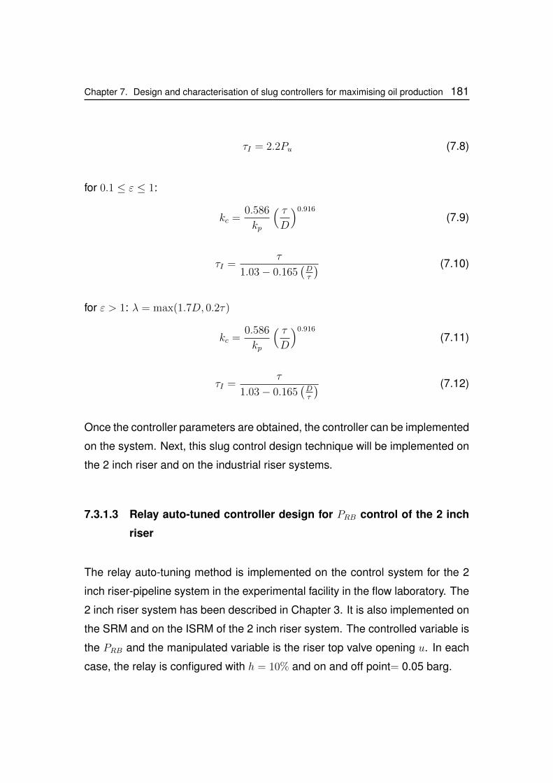
Chapter 7. Design and characterisation of slug controllers for maximising oil production 181
τI = 2.2Pu (7.8)
for 0.1 ≤ ε ≤ 1:
kc =0.586
kp
( τD
)0.916
(7.9)
τI =τ
1.03− 0.165(Dτ
) (7.10)
for ε > 1: λ = max(1.7D, 0.2τ)
kc =0.586
kp
( τD
)0.916
(7.11)
τI =τ
1.03− 0.165(Dτ
) (7.12)
Once the controller parameters are obtained, the controller can be implemented
on the system. Next, this slug control design technique will be implemented on
the 2 inch riser and on the industrial riser systems.
7.3.1.3 Relay auto-tuned controller design for PRB control of the 2 inch
riser
The relay auto-tuning method is implemented on the control system for the 2
inch riser-pipeline system in the experimental facility in the flow laboratory. The
2 inch riser system has been described in Chapter 3. It is also implemented on
the SRM and on the ISRM of the 2 inch riser system. The controlled variable is
the PRB and the manipulated variable is the riser top valve opening u. In each
case, the relay is configured with h = 10% and on and off point= 0.05 barg.
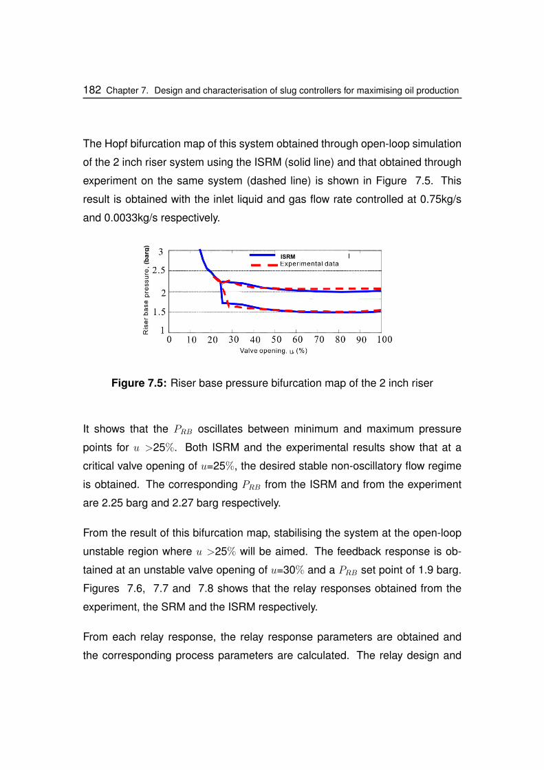
182 Chapter 7. Design and characterisation of slug controllers for maximising oil production
The Hopf bifurcation map of this system obtained through open-loop simulation
of the 2 inch riser system using the ISRM (solid line) and that obtained through
experiment on the same system (dashed line) is shown in Figure 7.5. This
result is obtained with the inlet liquid and gas flow rate controlled at 0.75kg/s
and 0.0033kg/s respectively.
ISRM
u
(ba
rg)
Figure 7.5: Riser base pressure bifurcation map of the 2 inch riser
It shows that the PRB oscillates between minimum and maximum pressure
points for u >25%. Both ISRM and the experimental results show that at a
critical valve opening of u=25%, the desired stable non-oscillatory flow regime
is obtained. The corresponding PRB from the ISRM and from the experiment
are 2.25 barg and 2.27 barg respectively.
From the result of this bifurcation map, stabilising the system at the open-loop
unstable region where u >25% will be aimed. The feedback response is ob-
tained at an unstable valve opening of u=30% and a PRB set point of 1.9 barg.
Figures 7.6, 7.7 and 7.8 shows that the relay responses obtained from the
experiment, the SRM and the ISRM respectively.
From each relay response, the relay response parameters are obtained and
the corresponding process parameters are calculated. The relay design and
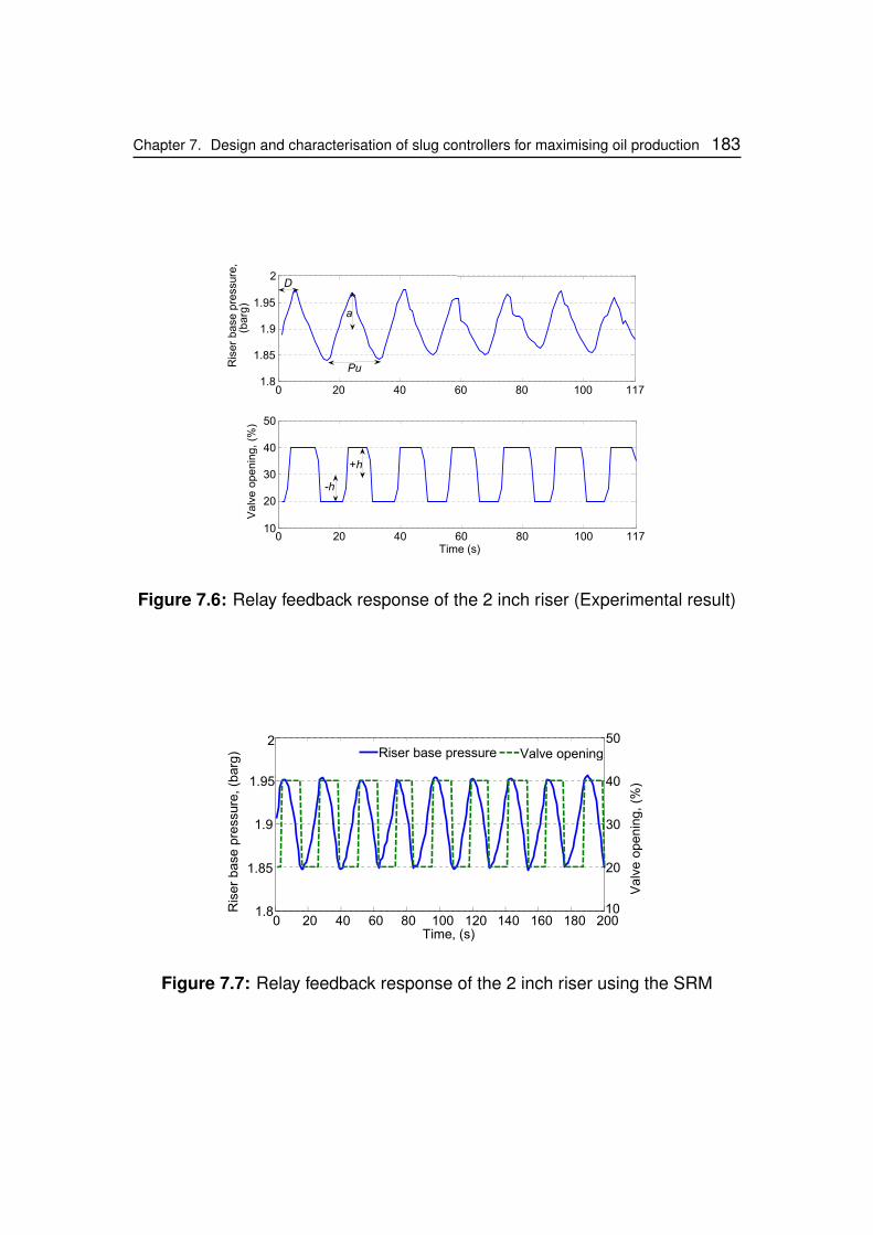
Chapter 7. Design and characterisation of slug controllers for maximising oil production 183
0 20 40 60 80 100 1171.8
1.85
1.9
1.95
2
Ris
er
base
pre
ssure
,(b
arg
)
0 20 40 60 80 100 11710
20
30
40
50
Time (s)
Valv
eopenin
g,
(%)
D
a
Pu
-h
+h
Figure 7.6: Relay feedback response of the 2 inch riser (Experimental result)
0 20 40 60 80 100 120 140 160 180 2001.8
1.85
1.9
1.95
2
Ris
er
base
pre
ssure
,(b
arg
)
10
20
30
40
50
Time, (s)
Valv
eopenin
g,
(%)
Valve openingRiser base pressure
Figure 7.7: Relay feedback response of the 2 inch riser using the SRM
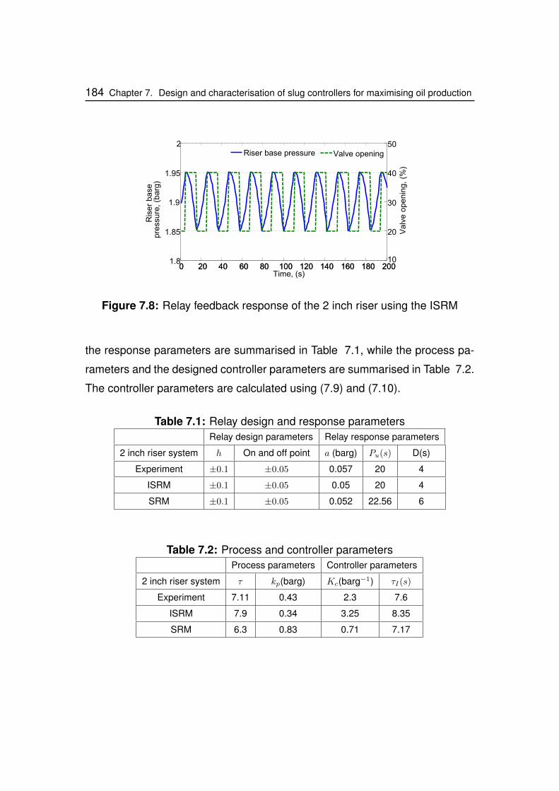
184 Chapter 7. Design and characterisation of slug controllers for maximising oil production
0 20 40 60 80 100 120 140 160 180 2001.8
1.85
1.9
1.95
2R
iser
base
pre
ssure
,(b
arg
)
0 20 40 60 80 100 120 140 160 180 20010
20
30
40
50
Time, (s)
Valv
eopenin
g,
(%)
Valve openingRiser base pressure
Figure 7.8: Relay feedback response of the 2 inch riser using the ISRM
the response parameters are summarised in Table 7.1, while the process pa-
rameters and the designed controller parameters are summarised in Table 7.2.
The controller parameters are calculated using (7.9) and (7.10).
Table 7.1: Relay design and response parametersRelay design parameters Relay response parameters
2 inch riser system h On and off point a (barg) Pu(s) D(s)
Experiment ±0.1 ±0.05 0.057 20 4
ISRM ±0.1 ±0.05 0.05 20 4
SRM ±0.1 ±0.05 0.052 22.56 6
Table 7.2: Process and controller parametersProcess parameters Controller parameters
2 inch riser system τ kp(barg) Kc(barg−1) τI(s)
Experiment 7.11 0.43 2.3 7.6
ISRM 7.9 0.34 3.25 8.35
SRM 6.3 0.83 0.71 7.17
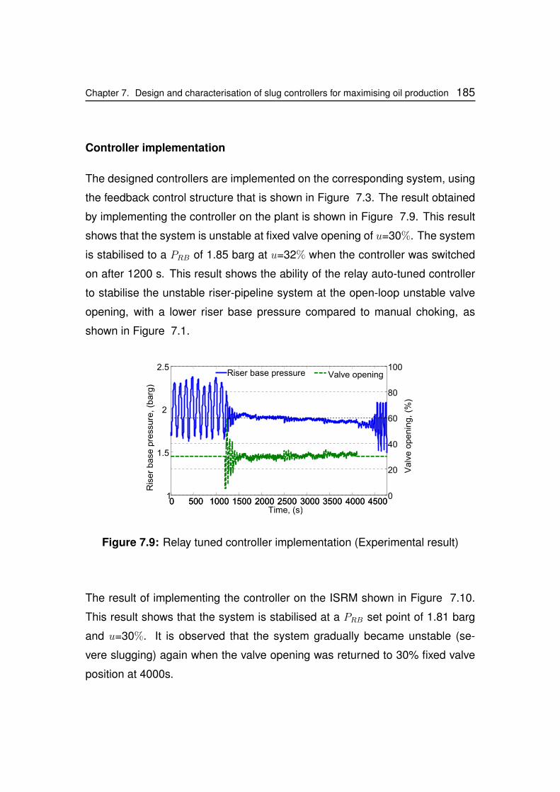
Chapter 7. Design and characterisation of slug controllers for maximising oil production 185
Controller implementation
The designed controllers are implemented on the corresponding system, using
the feedback control structure that is shown in Figure 7.3. The result obtained
by implementing the controller on the plant is shown in Figure 7.9. This result
shows that the system is unstable at fixed valve opening of u=30%. The system
is stabilised to a PRB of 1.85 barg at u=32% when the controller was switched
on after 1200 s. This result shows the ability of the relay auto-tuned controller
to stabilise the unstable riser-pipeline system at the open-loop unstable valve
opening, with a lower riser base pressure compared to manual choking, as
shown in Figure 7.1.
0 500 1000 1500 2000 2500 3000 3500 4000 45001
1.5
2
2.5
Time, (s)
Ris
er
base
pre
ssure
,(b
arg
)
0 500 1000 1500 2000 2500 3000 3500 4000 45000
20
40
60
80
100Valve openingRiser base pressure
Valv
eopenin
g,
(%)
Figure 7.9: Relay tuned controller implementation (Experimental result)
The result of implementing the controller on the ISRM shown in Figure 7.10.
This result shows that the system is stabilised at a PRB set point of 1.81 barg
and u=30%. It is observed that the system gradually became unstable (se-
vere slugging) again when the valve opening was returned to 30% fixed valve
position at 4000s.
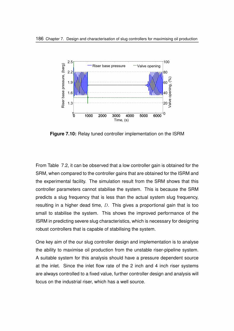
186 Chapter 7. Design and characterisation of slug controllers for maximising oil production
0 1000 2000 3000 4000 5000 60001
1.3
1.6
1.9
2.2
2.5
0 1000 2000 3000 4000 5000 60000
20
40
60
80
100
Time, (s)
Valv
eopenin
g,
(%)
Valve openingRiser base pressureR
iser
base
pre
ssure
,(b
arg
)
Figure 7.10: Relay tuned controller implementation on the ISRM
From Table 7.2, it can be observed that a low controller gain is obtained for the
SRM, when compared to the controller gains that are obtained for the ISRM and
the experimental facility. The simulation result from the SRM shows that this
controller parameters cannot stabilise the system. This is because the SRM
predicts a slug frequency that is less than the actual system slug frequency,
resulting in a higher dead time, D. This gives a proportional gain that is too
small to stabilise the system. This shows the improved performance of the
ISRM in predicting severe slug characteristics, which is necessary for designing
robust controllers that is capable of stabilising the system.
One key aim of the our slug controller design and implementation is to analyse
the ability to maximise oil production from the unstable riser-pipeline system.
A suitable system for this analysis should have a pressure dependent source
at the inlet. Since the inlet flow rate of the 2 inch and 4 inch riser systems
are always controlled to a fixed value, further controller design and analysis will
focus on the industrial riser, which has a well source.
Chapter 7. Design and characterisation of slug controllers for maximising oil production 187
7.3.1.4 Relay auto-tuned slug controller design for an industrial riser
To evaluate the performance of the relay auto-tuned active controller on severe
slugging control of larger scale riser-pipeline systems and on oil production, the
relay auto-tuned controller is implemented on the industrial riser system in the
OLGA software. With the industrial riser system, the production, which can be
achieved using the relay-tuned controller, can be evaluated since the industrial
riser system has a pressure driven well source. The relay auto-tuned controller
design is implemented for control using two controlled variables namely, the
PRB and the QT . The controller performance is analysed for each of the con-
trolled variable. With the flow condition given in Table 3.1, it is shown in Figure
4.18 that the industrial riser system is open-loop stable at u=12% and open-loop
unstable at u >13%.
Riser base pressure (PRB) control
In the relay auto-tuned slug controller design for PRB control, the system is
configured by setting the reference valve opening to the open-loop unstable
valve opening of u=20%. The relay is then designed using the relay design
parameters shown in Table 7.3. The feedback response obtained from the relay
test is shown in Figure 7.11, and the response parameters are summarised in
Table 7.3.
Table 7.3: Relay design and response parametersRelay design parameters Relay response parameters
Valve opening (%) h On and off point a (barg) Pu(s) D(s)
20% ±0.11 ±0.5 0.52 486 14.2
From this response, the system response parameters are obtained and the
process parameters calculated using (7.4) and (7.5). The controller parameters
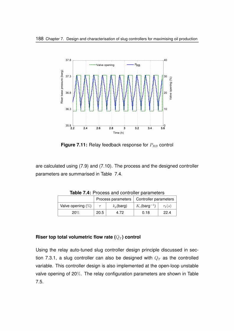
188 Chapter 7. Design and characterisation of slug controllers for maximising oil production
Time (h)
2.2 2.4 2.6 2.8 3 3.2 3.4 3.635.8
36.3
36.8
37.3
37.8R
iser
base
pre
ssure
(barg
)
2.2 2.4 2.6 2.8 3 3.2 3.4 3.60
10
20
30
40
PRBValve opening
Valv
eopenin
g(%
)
Figure 7.11: Relay feedback response for PRB control
are calculated using (7.9) and (7.10). The process and the designed controller
parameters are summarised in Table 7.4.
Table 7.4: Process and controller parametersProcess parameters Controller parameters
Valve opening (%) τ kp(barg) Kc(barg−1) τI(s)
20% 20.5 4.72 0.18 22.4
Riser top total volumetric flow rate (QT ) control
Using the relay auto-tuned slug controller design principle discussed in sec-
tion 7.3.1, a slug controller can also be designed with QT as the controlled
variable. This controller design is also implemented at the open-loop unstable
valve opening of 20%. The relay configuration parameters are shown in Table
7.5.
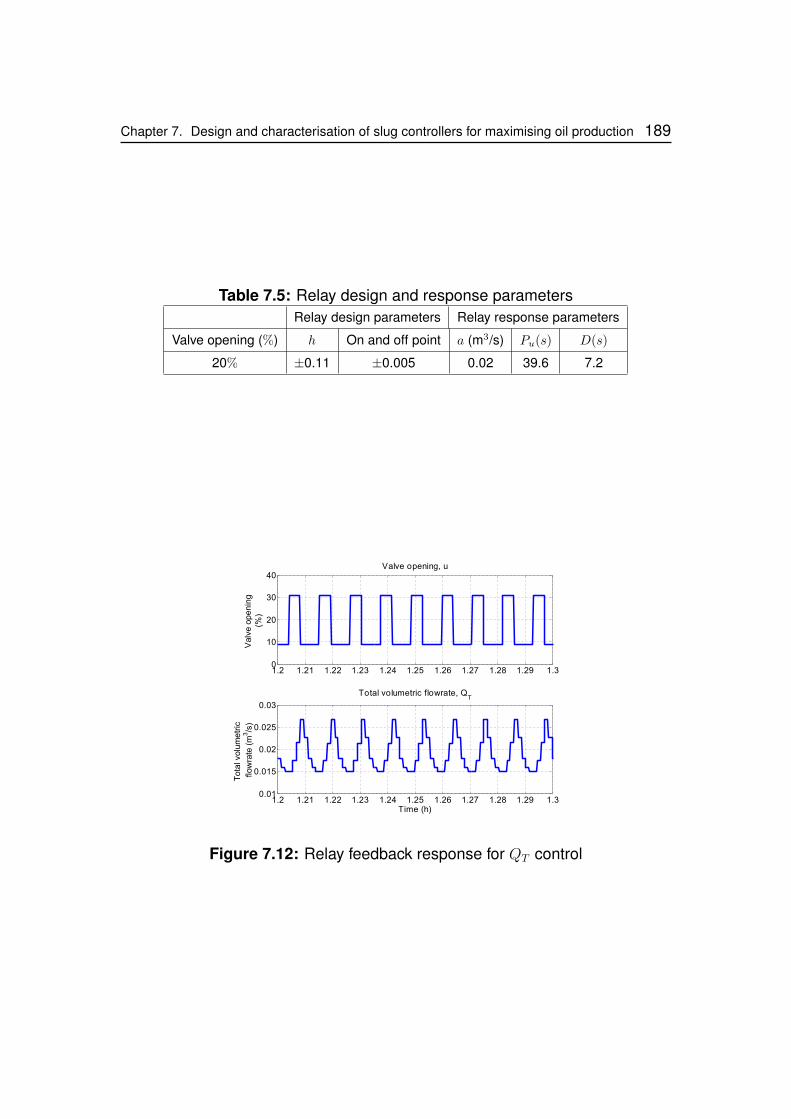
Chapter 7. Design and characterisation of slug controllers for maximising oil production 189
Table 7.5: Relay design and response parametersRelay design parameters Relay response parameters
Valve opening (%) h On and off point a (m3/s) Pu(s) D(s)
20% ±0.11 ±0.005 0.02 39.6 7.2
1.2 1.21 1.22 1.23 1.24 1.25 1.26 1.27 1.28 1.29 1.30
10
20
30
40Valve opening, u
Valv
eopenin
g(%
)
1.2 1.21 1.22 1.23 1.24 1.25 1.26 1.27 1.28 1.29 1.30.01
0.015
0.02
0.025
0.03
Total volumetric flowrate, QT
Tota
lvolu
metr
ic
flow
rate
(m3/s
)
Time (h)
Figure 7.12: Relay feedback response for QT control
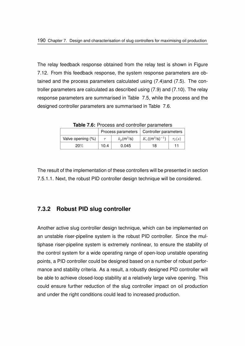
190 Chapter 7. Design and characterisation of slug controllers for maximising oil production
The relay feedback response obtained from the relay test is shown in Figure
7.12. From this feedback response, the system response parameters are ob-
tained and the process parameters calculated using (7.4)and (7.5). The con-
troller parameters are calculated as described using (7.9) and (7.10). The relay
response parameters are summarised in Table 7.5, while the process and the
designed controller parameters are summarised in Table 7.6.
Table 7.6: Process and controller parametersProcess parameters Controller parameters
Valve opening (%) τ kp(m3/s) Kc((m3/s)−1) τI(s)
20% 10.4 0.045 18 11
The result of the implementation of these controllers will be presented in section
7.5.1.1. Next, the robust PID controller design technique will be considered.
7.3.2 Robust PID slug controller
Another active slug controller design technique, which can be implemented on
an unstable riser-pipeline system is the robust PID controller. Since the mul-
tiphase riser-pipeline system is extremely nonlinear, to ensure the stability of
the control system for a wide operating range of open-loop unstable operating
points, a PID controller could be designed based on a number of robust perfor-
mance and stability criteria. As a result, a robustly designed PID controller will
be able to achieve closed-loop stability at a relatively large valve opening. This
could ensure further reduction of the slug controller impact on oil production
and under the right conditions could lead to increased production.
Chapter 7. Design and characterisation of slug controllers for maximising oil production 191
The design of a robust PID controller presented in this work requires a linear
model of the system obtained at an open-loop unstable valve opening. This lin-
ear model can be obtained using the ISRM of the relevant riser-pipeline system.
The principle of design of the robust PID controller is based on synthesising a
stabilising controller, which satisfy a number of relevant robust stability and per-
formance criteria. These robust performance and stability criteria are described
in the next section with a brief introduction of the feedback control structure.
7.3.2.1 Controller design criteria
Figure 7.13 gives a basic feedback control structure, which can be used to
synthesis the controller design criteria and implement the controller.
Figure 7.13: Feedback control loop diagram for severe slug control
In Figure 7.13, G is the transfer function of the riser-pipeline system obtained
through linearisation of the ISRM at the desired open-loop operating point, K
is the PID controller with transfer function given as:
K = Kc
(1 +
1
τis+ τDs
)(7.13)
192 Chapter 7. Design and characterisation of slug controllers for maximising oil production
where Kc is the controller gain, τI is the controller integral time and τD is
the controller derivative time. n represents uncertainties due to measurement
noise and modeling errors. Gd is the transfer function from disturbances to
PRB, where disturbances, d, include the liquid and gas flowrate variations, well
pressure and downstream (topside separator) pressure fluctuations. From Fig-
ure 7.13, the PRB of the riser-pipeline control system can be represented as:
PRB actual = Gu+Gdd (7.14)
Thus, the closed-loop response can be derived as:
PRB actual = TPRB setpoint + SGdd− Tn (7.15)
Where S = (1 + GK)−1 is known as the sensitivity function and T = GK(1 +
GK)−1 is known as the complementary sensitivity function. These sensitiv-
ity functions are used to define the criteria for robust PID controller design as
summarised below. The criteria used in determining suitable PID parameters
for robust stability are:
1. the upper bound on sensitivity function, |S|, which requires that S ≈ 0 or
T ≈ 1
2. the lower and upper bound on the loop gain, GK, which requires that
|G(jω)K(jω)| > 1 at lower frequencies below the cross over frequency
(ωc), and that |G(jω)K(jω)| is small, that is |G(jω)K(jω)| < 1 at higher
frequencies above the cross over frequencies
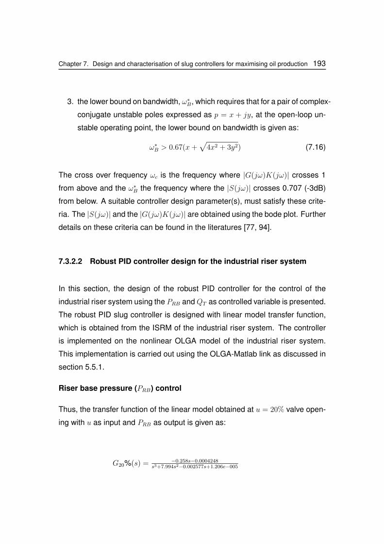
Chapter 7. Design and characterisation of slug controllers for maximising oil production 193
3. the lower bound on bandwidth, ω∗B, which requires that for a pair of complex-
conjugate unstable poles expressed as p = x + jy, at the open-loop un-
stable operating point, the lower bound on bandwidth is given as:
ω∗B > 0.67(x+√
4x2 + 3y2) (7.16)
The cross over frequency ωc is the frequency where |G(jω)K(jω)| crosses 1
from above and the ω∗B the frequency where the |S(jω)| crosses 0.707 (-3dB)
from below. A suitable controller design parameter(s), must satisfy these crite-
ria. The |S(jω)| and the |G(jω)K(jω)| are obtained using the bode plot. Further
details on these criteria can be found in the literatures [77, 94].
7.3.2.2 Robust PID controller design for the industrial riser system
In this section, the design of the robust PID controller for the control of the
industrial riser system using the PRB andQT as controlled variable is presented.
The robust PID slug controller is designed with linear model transfer function,
which is obtained from the ISRM of the industrial riser system. The controller
is implemented on the nonlinear OLGA model of the industrial riser system.
This implementation is carried out using the OLGA-Matlab link as discussed in
section 5.5.1.
Riser base pressure (PRB) control
Thus, the transfer function of the linear model obtained at u = 20% valve open-
ing with u as input and PRB as output is given as:
G20%(s) = −0.258s−0.0004248s3+7.994s2−0.002577s+1.206e−005
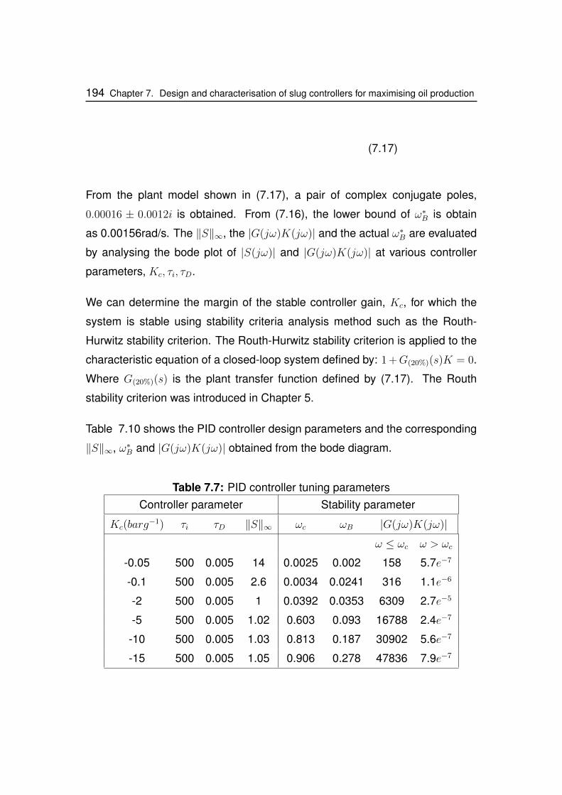
194 Chapter 7. Design and characterisation of slug controllers for maximising oil production
(7.17)
From the plant model shown in (7.17), a pair of complex conjugate poles,
0.00016 ± 0.0012i is obtained. From (7.16), the lower bound of ω∗B is obtain
as 0.00156rad/s. The ‖S‖∞, the |G(jω)K(jω)| and the actual ω∗B are evaluated
by analysing the bode plot of |S(jω)| and |G(jω)K(jω)| at various controller
parameters, Kc, τi, τD.
We can determine the margin of the stable controller gain, Kc, for which the
system is stable using stability criteria analysis method such as the Routh-
Hurwitz stability criterion. The Routh-Hurwitz stability criterion is applied to the
characteristic equation of a closed-loop system defined by: 1 +G(20%)(s)K = 0.
Where G(20%)(s) is the plant transfer function defined by (7.17). The Routh
stability criterion was introduced in Chapter 5.
Table 7.10 shows the PID controller design parameters and the corresponding
‖S‖∞, ω∗B and |G(jω)K(jω)| obtained from the bode diagram.
Table 7.7: PID controller tuning parametersController parameter Stability parameter
Kc(barg−1) τi τD ‖S‖∞ ωc ωB |G(jω)K(jω)|
ω ≤ ωc ω > ωc
-0.05 500 0.005 14 0.0025 0.002 158 5.7e−7
-0.1 500 0.005 2.6 0.0034 0.0241 316 1.1e−6
-2 500 0.005 1 0.0392 0.0353 6309 2.7e−5
-5 500 0.005 1.02 0.603 0.093 16788 2.4e−7
-10 500 0.005 1.03 0.813 0.187 30902 5.6e−7
-15 500 0.005 1.05 0.906 0.278 47836 7.9e−7
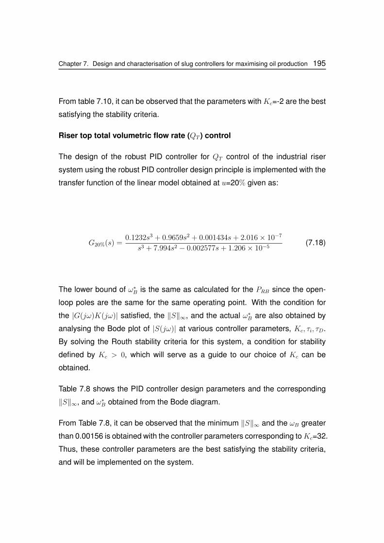
Chapter 7. Design and characterisation of slug controllers for maximising oil production 195
From table 7.10, it can be observed that the parameters with Kc=-2 are the best
satisfying the stability criteria.
Riser top total volumetric flow rate (QT ) control
The design of the robust PID controller for QT control of the industrial riser
system using the robust PID controller design principle is implemented with the
transfer function of the linear model obtained at u=20% given as:
G20%(s) =0.1232s3 + 0.9659s2 + 0.001434s+ 2.016× 10⁻⁷
s3 + 7.994s2 − 0.002577s+ 1.206× 10⁻⁵(7.18)
The lower bound of ω∗B is the same as calculated for the PRB since the open-
loop poles are the same for the same operating point. With the condition for
the |G(jω)K(jω)| satisfied, the ‖S‖∞, and the actual ω∗B are also obtained by
analysing the Bode plot of |S(jω)| at various controller parameters, Kc, τi, τD.
By solving the Routh stability criteria for this system, a condition for stability
defined by Kc > 0, which will serve as a guide to our choice of Kc can be
obtained.
Table 7.8 shows the PID controller design parameters and the corresponding
‖S‖∞, and ω∗B obtained from the Bode diagram.
From Table 7.8, it can be observed that the minimum ‖S‖∞ and the ωB greater
than 0.00156 is obtained with the controller parameters corresponding toKc=32.
Thus, these controller parameters are the best satisfying the stability criteria,
and will be implemented on the system.
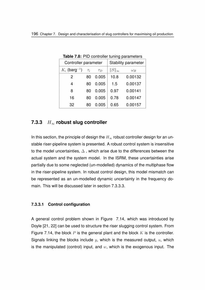
196 Chapter 7. Design and characterisation of slug controllers for maximising oil production
Table 7.8: PID controller tuning parametersController parameter Stability parameter
Kc (barg−1) τi τD ‖S‖∞ ωB
2 80 0.005 10.8 0.00132
4 80 0.005 1.5 0.00137
8 80 0.005 0.97 0.00141
16 80 0.005 0.78 0.00147
32 80 0.005 0.65 0.00157
7.3.3 H∞ robust slug controller
In this section, the principle of design the H∞ robust controller design for an un-
stable riser-pipeline system is presented. A robust control system is insensitive
to the model uncertainties, ∆ , which arise due to the differences between the
actual system and the system model. In the ISRM, these uncertainties arise
partially due to some neglected (un-modelled) dynamics of the multiphase flow
in the riser-pipeline system. In robust control design, this model mismatch can
be represented as an un-modelled dynamic uncertainty in the frequency do-
main. This will be discussed later in section 7.3.3.3.
7.3.3.1 Control configuration
A general control problem shown in Figure 7.14, which was introduced by
Doyle [21, 22] can be used to structure the riser slugging control system. From
Figure 7.14, the block P is the general plant and the block K is the controller.
Signals linking the blocks include y, which is the measured output, u, which
is the manipulated (control) input, and w, which is the exogenous input. The
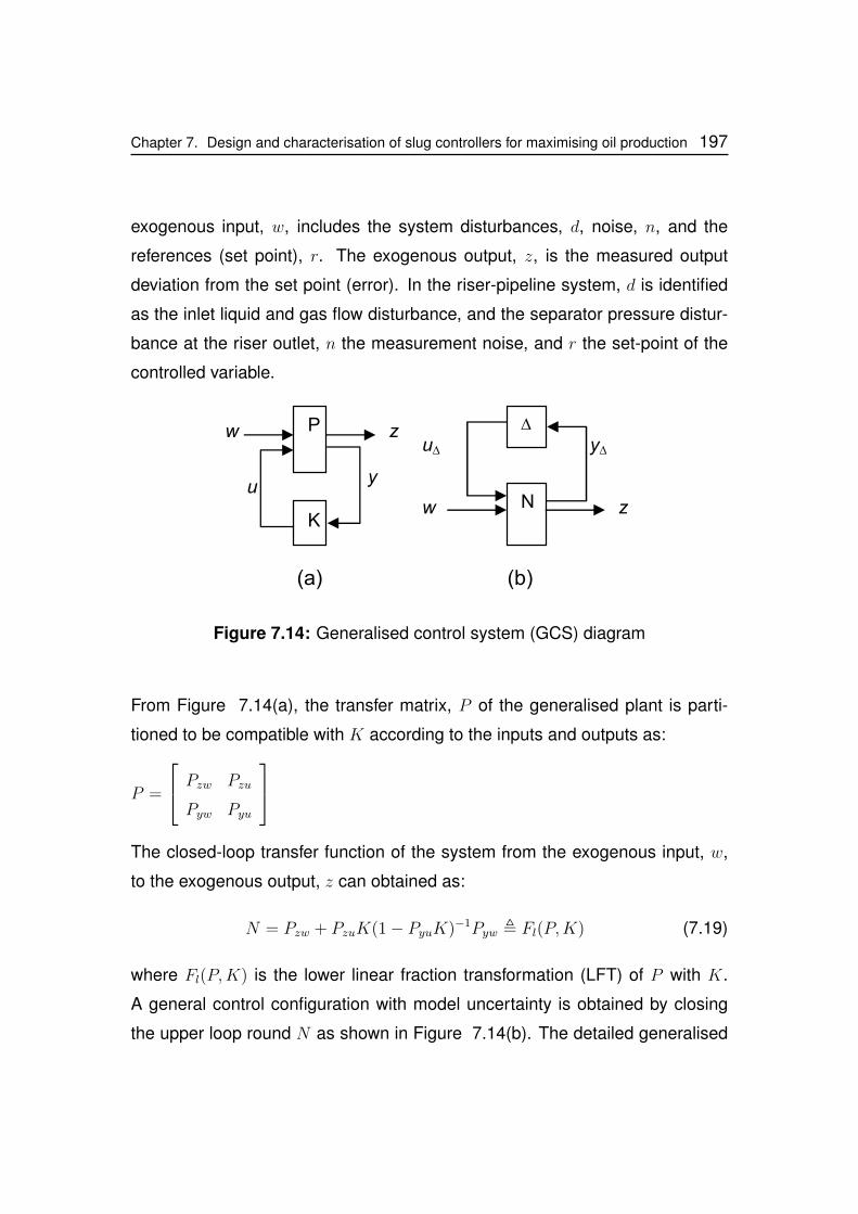
Chapter 7. Design and characterisation of slug controllers for maximising oil production 197
exogenous input, w, includes the system disturbances, d, noise, n, and the
references (set point), r. The exogenous output, z, is the measured output
deviation from the set point (error). In the riser-pipeline system, d is identified
as the inlet liquid and gas flow disturbance, and the separator pressure distur-
bance at the riser outlet, n the measurement noise, and r the set-point of the
controlled variable.
P
K
w z
yu
N
∆
w z
y∆u∆
(a) (b)
Figure 7.14: Generalised control system (GCS) diagram
From Figure 7.14(a), the transfer matrix, P of the generalised plant is parti-
tioned to be compatible with K according to the inputs and outputs as:
P =
Pzw Pzu
Pyw Pyu
The closed-loop transfer function of the system from the exogenous input, w,
to the exogenous output, z can obtained as:
N = Pzw + PzuK(1− PyuK)−1Pyw , Fl(P,K) (7.19)
where Fl(P,K) is the lower linear fraction transformation (LFT) of P with K.
A general control configuration with model uncertainty is obtained by closing
the upper loop round N as shown in Figure 7.14(b). The detailed generalised
198 Chapter 7. Design and characterisation of slug controllers for maximising oil production
control structure was shown in Figure 7.2. Considering the system uncertainty,
the close loop transfer function from w to z results in an upper LFT, F , given as:
F = Fu(N,4) := Nzw +NzuM 4 (1−NyMuM4)−1NyMw (7.20)
From Figure 7.2, the partitioned generalised plant,P , from the inputs [uM r n d u]T
to the outputs [yM z1 z2 y]T is derived as:
P =
0 0 0 0 WI
−WpG WpR −WpNs −WpGd −WpG
0 0 0 0 Wu
−G R −Ns −Gd −G
Thus, from (7.19), N , which is the transfer function from w to z is derived as:−WIKSG WIKSR −WIKSNs −WIKSGd
−WpSG WpSR −WpSNs −WpSGd
−WuKSG WuKSR −WuKSNs −WuKSGd
Controller synthesis based on this generalised control configuration can be ap-
plied to an open-loop unstable robust controller design for severe slug mitiga-
tion.
7.3.3.2 Controller design criteria
The control objective in terms of quantitative performance criteria is to minimise
various norms of the system, such as the H∞ norm from w, to z [12]. The
H∞ optimal control problem aims to find a stabilising controller, K, such that
‖Fl(P,K)‖∞ = maxω σ(Fl(P,K)(jω)) is minimised. If min ‖Fl(P,K)‖∞ = γmin,
then usually, a theoretically simpler design is to obtain a sub-optimal controller
with γ > γmin.
Chapter 7. Design and characterisation of slug controllers for maximising oil production 199
Thus, the control problem would be to find a stabilizing controller such that
‖Fl(P,K)‖∞ < γ. Such controllers should satisfy the performance and robust
stability conditions as described below.
Robust performance
The sensitivity function of the perturbed system, Sp(s) = (1 + Gp(s)K(s))−1 is
typically a good indicator of closed-loop performance of a system. The maxi-
mum peak amplitude of Sp is usually selected such that ‖Sp‖∞ ≤ 2. This perfor-
mance specification can be represented by a performance weight, Wp, which
places an upper bound, 1|Wp(s)| , on the magnitude of Sp. Thus, the performance
requirement becomes |Sp(jω)| < 1/|Wp(jω)|,∀ω such that ‖Wp(jω)Sp(jω)‖∞.
In terms of the H∞ norm, this performance requirement demands from (7.20)
that, F ≤ 1,∀4, ‖4‖∞ ≤ 1 [76]. Wp(s) is defined as Wp(s) =s/M+ω∗Bs+ω∗BA
where
ω∗B is the bandwidth requirement. |S(jω)| ≤ M is required for high frequency
performance above the bandwidth and |S(0)| ≤ A is the steady state offset
required for low frequency performance.
Robust stability
To evaluate robust stability of a system, we determine if the system is stable for
all plants in the uncertainty set, that is, F = Fu(N,4) is stable ∀4, ‖4‖∞ ≤ 1.
Nominal stability, NS, is required as a prerequisite for robust stability of F . NS
demands that N is internally stable, so that the only source of instability in F is
the feedback loop (1 − NyMuM4)−1 introduced by the uncertainty, 4 as shown
in (7.20). NyMuM is the closed-loop transfer function from u4 to y4, which is
obtained as −WIKSG = −WIT from N . By analysing the Nyquist plot of
the loop transfer function with uncertainty, Lp , the robust stability condition is,|WI(jω)L(jω)||1+L(jω)| < 1,∀ω ⇔ |WI(jω)T (jω)| < 1,∀ω. Thus, from N , it is required that
|NyMuM | = |WI(jω)T (jω)| < 1,∀ω,∀4, ‖4‖∞ ≤ 1, to achieve robust stability.
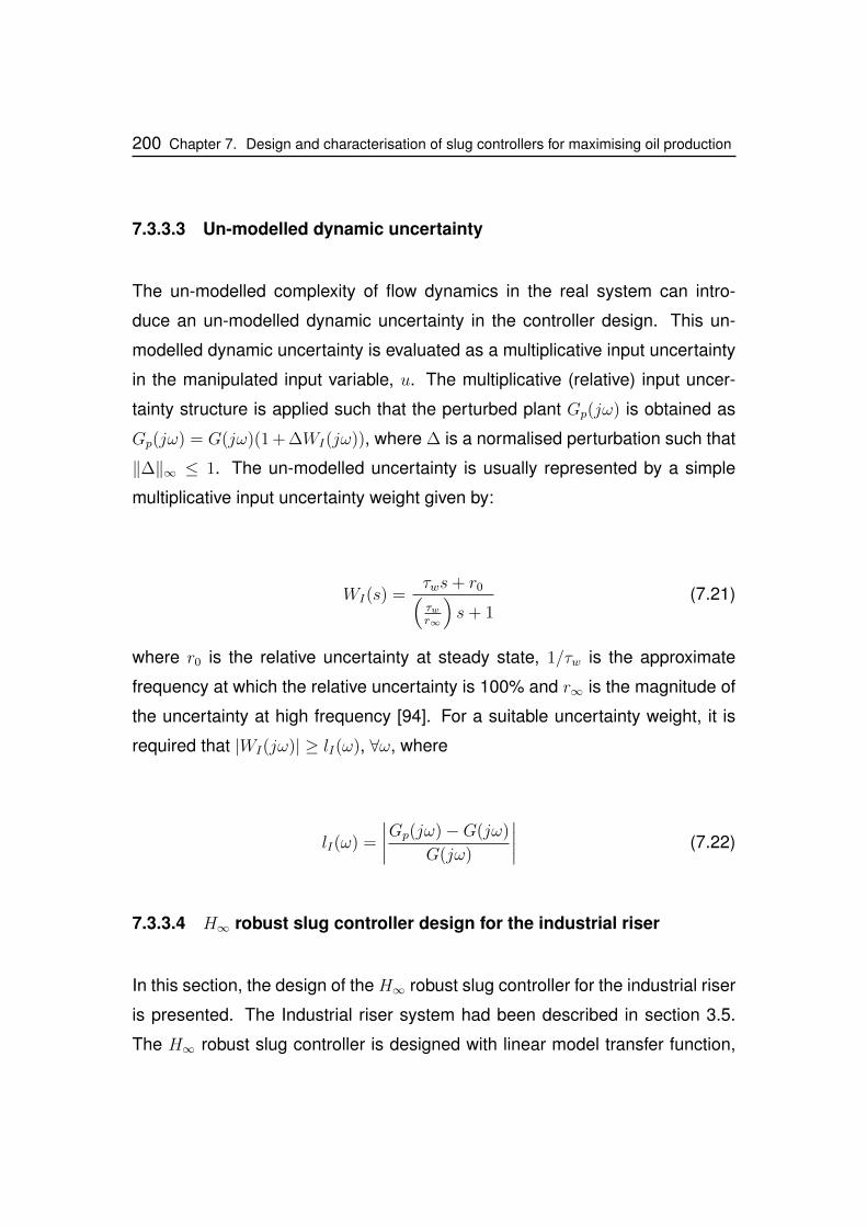
200 Chapter 7. Design and characterisation of slug controllers for maximising oil production
7.3.3.3 Un-modelled dynamic uncertainty
The un-modelled complexity of flow dynamics in the real system can intro-
duce an un-modelled dynamic uncertainty in the controller design. This un-
modelled dynamic uncertainty is evaluated as a multiplicative input uncertainty
in the manipulated input variable, u. The multiplicative (relative) input uncer-
tainty structure is applied such that the perturbed plant Gp(jω) is obtained as
Gp(jω) = G(jω)(1 + ∆WI(jω)), where ∆ is a normalised perturbation such that
‖∆‖∞ ≤ 1. The un-modelled uncertainty is usually represented by a simple
multiplicative input uncertainty weight given by:
WI(s) =τws+ r0(τwr∞
)s+ 1
(7.21)
where r0 is the relative uncertainty at steady state, 1/τw is the approximate
frequency at which the relative uncertainty is 100% and r∞ is the magnitude of
the uncertainty at high frequency [94]. For a suitable uncertainty weight, it is
required that |WI(jω)| ≥ lI(ω), ∀ω, where
lI(ω) =
∣∣∣∣Gp(jω)−G(jω)
G(jω)
∣∣∣∣ (7.22)
7.3.3.4 H∞ robust slug controller design for the industrial riser
In this section, the design of the H∞ robust slug controller for the industrial riser
is presented. The Industrial riser system had been described in section 3.5.
The H∞ robust slug controller is designed with linear model transfer function,
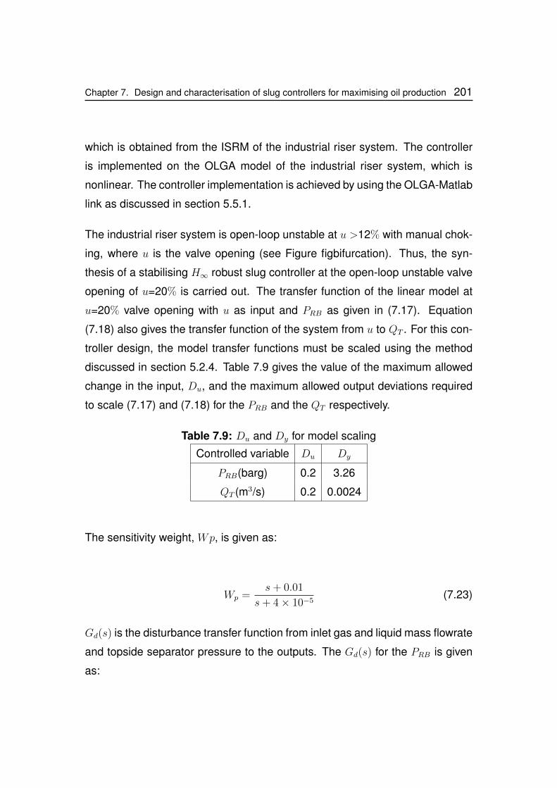
Chapter 7. Design and characterisation of slug controllers for maximising oil production 201
which is obtained from the ISRM of the industrial riser system. The controller
is implemented on the OLGA model of the industrial riser system, which is
nonlinear. The controller implementation is achieved by using the OLGA-Matlab
link as discussed in section 5.5.1.
The industrial riser system is open-loop unstable at u >12% with manual chok-
ing, where u is the valve opening (see Figure figbifurcation). Thus, the syn-
thesis of a stabilising H∞ robust slug controller at the open-loop unstable valve
opening of u=20% is carried out. The transfer function of the linear model at
u=20% valve opening with u as input and PRB as given in (7.17). Equation
(7.18) also gives the transfer function of the system from u to QT . For this con-
troller design, the model transfer functions must be scaled using the method
discussed in section 5.2.4. Table 7.9 gives the value of the maximum allowed
change in the input, Du, and the maximum allowed output deviations required
to scale (7.17) and (7.18) for the PRB and the QT respectively.
Table 7.9: Du and Dy for model scaling
Controlled variable Du Dy
PRB(barg) 0.2 3.26
QT (m3/s) 0.2 0.0024
The sensitivity weight, Wp, is given as:
Wp =s+ 0.01
s+ 4× 10⁻⁵(7.23)
Gd(s) is the disturbance transfer function from inlet gas and liquid mass flowrate
and topside separator pressure to the outputs. The Gd(s) for the PRB is given
as:
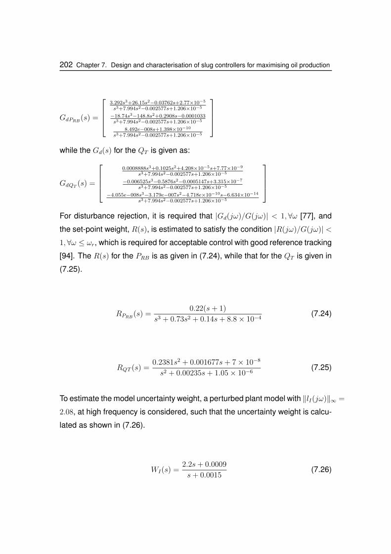
202 Chapter 7. Design and characterisation of slug controllers for maximising oil production
GdPRB(s) =
3.292s3+26.15s2−0.03762s+2.77×10⁻⁵
s3+7.994s2−0.002577s+1.206×10⁻⁵
−18.74s3−148.8s2+0.2908s−0.0001033s3+7.994s2−0.002577s+1.206×10⁻⁵
8.492e−008s+1.398×10⁻¹⁰
s3+7.994s2−0.002577s+1.206×10⁻⁵
while the Gd(s) for the QT is given as:
GdQT (s) =
0.0008888s3+0.1025s2+4.208×10⁻⁵s+7.77×10⁻⁹
s3+7.994s2−0.002577s+1.206×10⁻⁵
−0.006525s3−0.5876s2−0.0005147s+3.315×10⁻⁷
s3+7.994s2−0.002577s+1.206×10⁻⁵
−4.055e−008s3−3.179e−007s2−4.718e×10−10s−6.634×10⁻¹⁴
s3+7.994s2−0.002577s+1.206×10⁻⁵
For disturbance rejection, it is required that |Gd(jω)/G(jω)| < 1,∀ω [77], and
the set-point weight, R(s), is estimated to satisfy the condition |R(jω)/G(jω)| <1,∀ω ≤ ωr, which is required for acceptable control with good reference tracking
[94]. The R(s) for the PRB is as given in (7.24), while that for the QT is given in
(7.25).
RPRB(s) =0.22(s+ 1)
s3 + 0.73s2 + 0.14s+ 8.8× 10⁻⁴(7.24)
RQT (s) =0.2381s2 + 0.001677s+ 7× 10⁻⁸
s2 + 0.00235s+ 1.05× 10⁻⁶(7.25)
To estimate the model uncertainty weight, a perturbed plant model with ‖lI(jω)‖∞ =
2.08, at high frequency is considered, such that the uncertainty weight is calcu-
lated as shown in (7.26).
WI(s) =2.2s+ 0.0009
s+ 0.0015(7.26)
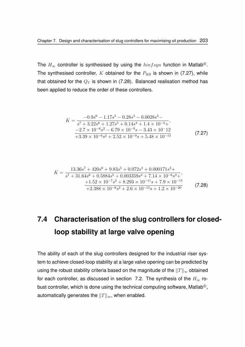
Chapter 7. Design and characterisation of slug controllers for maximising oil production 203
The H∞ controller is synthesised by using the hinfsyn function in Matlabr.
The synthesised controller, K obtained for the PRB is shown in (7.27), while
that obtained for the QT is shown in (7.28). Balanced realisation method has
been applied to reduce the order of these controllers.
K =−0.9s6 − 1.17s5 − 0.28s4 − 0.0028s3−
s7 + 3.22s6 + 1.27s5 + 0.14s4 + 1.4× 10⁻³+,
−2.7× 10⁻⁶s2 − 6.79× 10⁻⁹s− 3.43× 10⁻¹²
+3.39× 10⁻⁶s2 + 2.52× 10⁻⁹s+ 5.48× 10⁻¹³(7.27)
K =13.36s7 + 420s6 + 9.83s5 + 0.072s4 + 0.000171s3+
s7 + 31.64s6 + 0.5884s5 + 0.003359s4 + 7.14× 10⁻⁶s3+,
+1.52× 10⁻⁷s2 + 8.293× 10⁻¹¹s+ 7.9× 10⁻¹⁵
+2.388× 10⁻⁹s2 + 2.6× 10⁻¹³s+ 1.2× 10⁻²⁰(7.28)
7.4 Characterisation of the slug controllers for closed-
loop stability at large valve opening
The ability of each of the slug controllers designed for the industrial riser sys-
tem to achieve closed-loop stability at a large valve opening can be predicted by
using the robust stability criteria based on the magnitude of the ‖T‖∞ obtained
for each controller, as discussed in section 7.2. The synthesis of the H∞ ro-
bust controller, which is done using the technical computing software, Matlabr,
automatically generates the ‖T‖∞, when enabled.
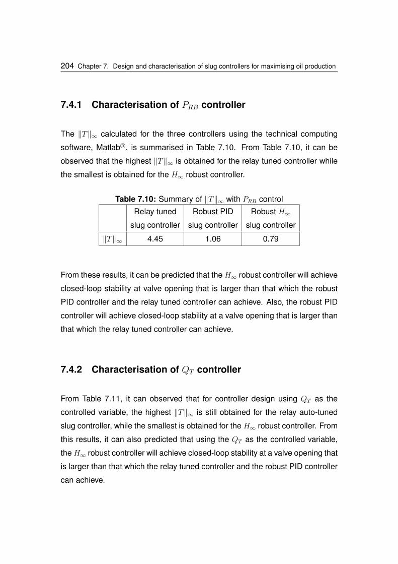
204 Chapter 7. Design and characterisation of slug controllers for maximising oil production
7.4.1 Characterisation of PRB controller
The ‖T‖∞ calculated for the three controllers using the technical computing
software, Matlabr, is summarised in Table 7.10. From Table 7.10, it can be
observed that the highest ‖T‖∞ is obtained for the relay tuned controller while
the smallest is obtained for the H∞ robust controller.
Table 7.10: Summary of ‖T‖∞ with PRB control
Relay tuned Robust PID Robust H∞slug controller slug controller slug controller
‖T‖∞ 4.45 1.06 0.79
From these results, it can be predicted that the H∞ robust controller will achieve
closed-loop stability at valve opening that is larger than that which the robust
PID controller and the relay tuned controller can achieve. Also, the robust PID
controller will achieve closed-loop stability at a valve opening that is larger than
that which the relay tuned controller can achieve.
7.4.2 Characterisation of QT controller
From Table 7.11, it can observed that for controller design using QT as the
controlled variable, the highest ‖T‖∞ is still obtained for the relay auto-tuned
slug controller, while the smallest is obtained for the H∞ robust controller. From
this results, it can also predicted that using the QT as the controlled variable,
theH∞ robust controller will achieve closed-loop stability at a valve opening that
is larger than that which the relay tuned controller and the robust PID controller
can achieve.
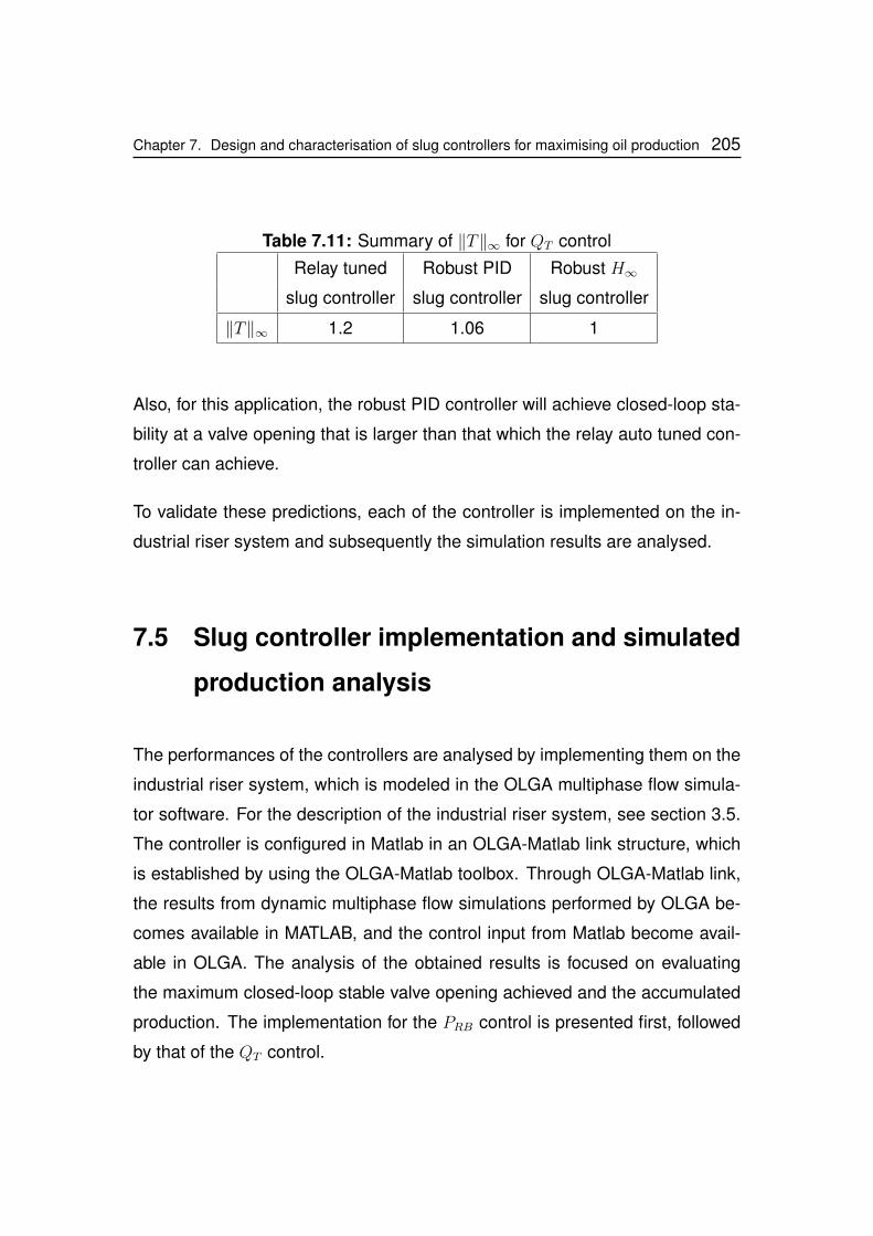
Chapter 7. Design and characterisation of slug controllers for maximising oil production 205
Table 7.11: Summary of ‖T‖∞ for QT control
Relay tuned Robust PID Robust H∞slug controller slug controller slug controller
‖T‖∞ 1.2 1.06 1
Also, for this application, the robust PID controller will achieve closed-loop sta-
bility at a valve opening that is larger than that which the relay auto tuned con-
troller can achieve.
To validate these predictions, each of the controller is implemented on the in-
dustrial riser system and subsequently the simulation results are analysed.
7.5 Slug controller implementation and simulated
production analysis
The performances of the controllers are analysed by implementing them on the
industrial riser system, which is modeled in the OLGA multiphase flow simula-
tor software. For the description of the industrial riser system, see section 3.5.
The controller is configured in Matlab in an OLGA-Matlab link structure, which
is established by using the OLGA-Matlab toolbox. Through OLGA-Matlab link,
the results from dynamic multiphase flow simulations performed by OLGA be-
comes available in MATLAB, and the control input from Matlab become avail-
able in OLGA. The analysis of the obtained results is focused on evaluating
the maximum closed-loop stable valve opening achieved and the accumulated
production. The implementation for the PRB control is presented first, followed
by that of the QT control.
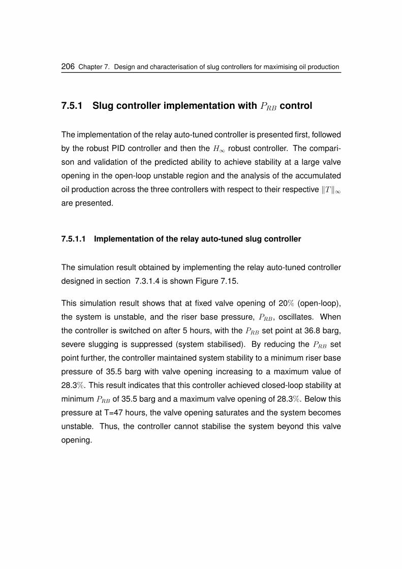
206 Chapter 7. Design and characterisation of slug controllers for maximising oil production
7.5.1 Slug controller implementation with PRB control
The implementation of the relay auto-tuned controller is presented first, followed
by the robust PID controller and then the H∞ robust controller. The compari-
son and validation of the predicted ability to achieve stability at a large valve
opening in the open-loop unstable region and the analysis of the accumulated
oil production across the three controllers with respect to their respective ‖T‖∞are presented.
7.5.1.1 Implementation of the relay auto-tuned slug controller
The simulation result obtained by implementing the relay auto-tuned controller
designed in section 7.3.1.4 is shown Figure 7.15.
This simulation result shows that at fixed valve opening of 20% (open-loop),
the system is unstable, and the riser base pressure, PRB, oscillates. When
the controller is switched on after 5 hours, with the PRB set point at 36.8 barg,
severe slugging is suppressed (system stabilised). By reducing the PRB set
point further, the controller maintained system stability to a minimum riser base
pressure of 35.5 barg with valve opening increasing to a maximum value of
28.3%. This result indicates that this controller achieved closed-loop stability at
minimum PRB of 35.5 barg and a maximum valve opening of 28.3%. Below this
pressure at T=47 hours, the valve opening saturates and the system becomes
unstable. Thus, the controller cannot stabilise the system beyond this valve
opening.
Chapter 7. Design and characterisation of slug controllers for maximising oil production 207
0 5 10 15 20 25 30 35 40 45 500
20
40
60
80
100Valveopening
Valv
eopenin
g(%
)
0 5 10 15 20 25 30 35 40 45 5030
35
40
45Riser basepressure
Ris
erbase
pre
ssure
(barg
)
Time(h)
PRB
PRB
setpoint
Figure 7.15: Slug control with relay tuned controller
Simulated production analysis
Figure 7.16 shows that the implementation of the relay controller at u=20%
yielded an accumulated oil production of 324.6 m3/day and 338 m3/day at
u=28.3%. This implies that with this controller, a 15% increase in production
at u=20%, and a 19.5% increase in production at u=28.3% can be achieved,
when compared to production obtained using manual choking.
Comparing this to the accumulated production with no control (severe slug-
ging) at u=20%, it can be observed that there is a 7% increase in production
with the controller. It is evident that with the open-loop unstable controller tun-
ing method, the relay tuned active slug control can meet the two fundamental
objectives of slug control, namely: stabilising the system (at a higher valve
opening other than the open-loop stable valve opening), and increasing oil pro-
duction.
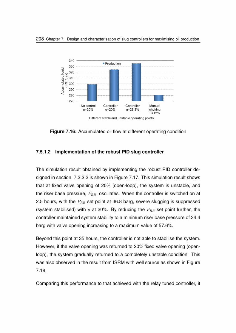
208 Chapter 7. Design and characterisation of slug controllers for maximising oil production
270
280
290
300
310
320
330
340
No controlu=20%
Controlleru=20%
Controlleru=28.3%
Manualchokingu=12%
Accum
ula
ted
liquid
(m3
/day)
Different stable and unstable operating points
Production
Figure 7.16: Accumulated oil flow at different operating condition
7.5.1.2 Implementation of the robust PID slug controller
The simulation result obtained by implementing the robust PID controller de-
signed in section 7.3.2.2 is shown in Figure 7.17. This simulation result shows
that at fixed valve opening of 20% (open-loop), the system is unstable, and
the riser base pressure, PRB, oscillates. When the controller is switched on at
2.5 hours, with the PRB set point at 36.8 barg, severe slugging is suppressed
(system stabilised) with u at 20%. By reducing the PRB set point further, the
controller maintained system stability to a minimum riser base pressure of 34.4
barg with valve opening increasing to a maximum value of 57.6%.
Beyond this point at 35 hours, the controller is not able to stabilise the system.
However, if the valve opening was returned to 20% fixed valve opening (open-
loop), the system gradually returned to a completely unstable condition. This
was also observed in the result from ISRM with well source as shown in Figure
7.18.
Comparing this performance to that achieved with the relay tuned controller, it

Chapter 7. Design and characterisation of slug controllers for maximising oil production 209
0 5 10 15 20 25 30 35 40 450
20
40
60
80
100Valve opening
Time (h)
Va
lve
op
enin
g(%
)
0 5 10 15 20 25 30 35 40 4530
35
40
45Riser base pressure
Ris
erb
ase
pre
ssu
re(b
arg
)
Prb set point
Prb
Figure 7.17: Slug control with robust PID controller - OLGA simulation
0 1 2 3 4 5 6 7
x 104
020406080
100
Va
lve
open
ing
(%)
0 1 2 3 4 5 6 7
x 104
353739414345
Ris
erb
ase
pre
ssu
re(b
arg
)Valve opening
0 1 2 3 4 5 6 7
x 104
0
10
20
30
40
Time (s)
Ris
erto
pto
tal
ma
ssfl
ow
rate
(kg
/s)
0 1 2 3 4 5 6 7
x 104
3
3.5
4
4.5
5
Figure 6: Severe slugging controlled at open loop unstableoperating point (SRSM simulation of the generic riser model)
Wel
lli
qu
idm
ass
flow
rate
(kg
/s)
Riser top total mass flowrate
Well liquid mass flowrate
PRB
Time (s)
Figure 7.18: Slug control with robust PID controller - ISRM simulation
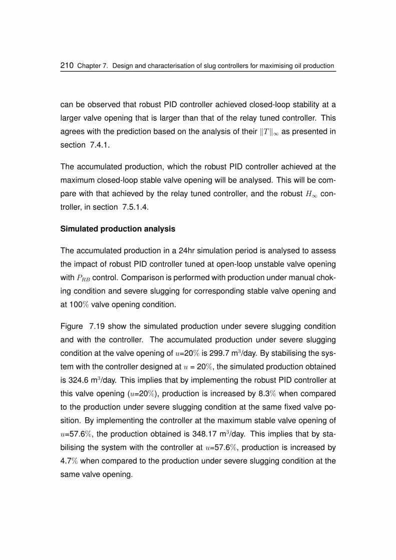
210 Chapter 7. Design and characterisation of slug controllers for maximising oil production
can be observed that robust PID controller achieved closed-loop stability at a
larger valve opening that is larger than that of the relay tuned controller. This
agrees with the prediction based on the analysis of their ‖T‖∞ as presented in
section 7.4.1.
The accumulated production, which the robust PID controller achieved at the
maximum closed-loop stable valve opening will be analysed. This will be com-
pare with that achieved by the relay tuned controller, and the robust H∞ con-
troller, in section 7.5.1.4.
Simulated production analysis
The accumulated production in a 24hr simulation period is analysed to assess
the impact of robust PID controller tuned at open-loop unstable valve opening
with PRB control. Comparison is performed with production under manual chok-
ing condition and severe slugging for corresponding stable valve opening and
at 100% valve opening condition.
Figure 7.19 show the simulated production under severe slugging condition
and with the controller. The accumulated production under severe slugging
condition at the valve opening of u=20% is 299.7 m3/day. By stabilising the sys-
tem with the controller designed at u = 20%, the simulated production obtained
is 324.6 m3/day. This implies that by implementing the robust PID controller at
this valve opening (u=20%), production is increased by 8.3% when compared
to the production under severe slugging condition at the same fixed valve po-
sition. By implementing the controller at the maximum stable valve opening of
u=57.6%, the production obtained is 348.17 m3/day. This implies that by sta-
bilising the system with the controller at u=57.6%, production is increased by
4.7% when compared to the production under severe slugging condition at the
same valve opening.
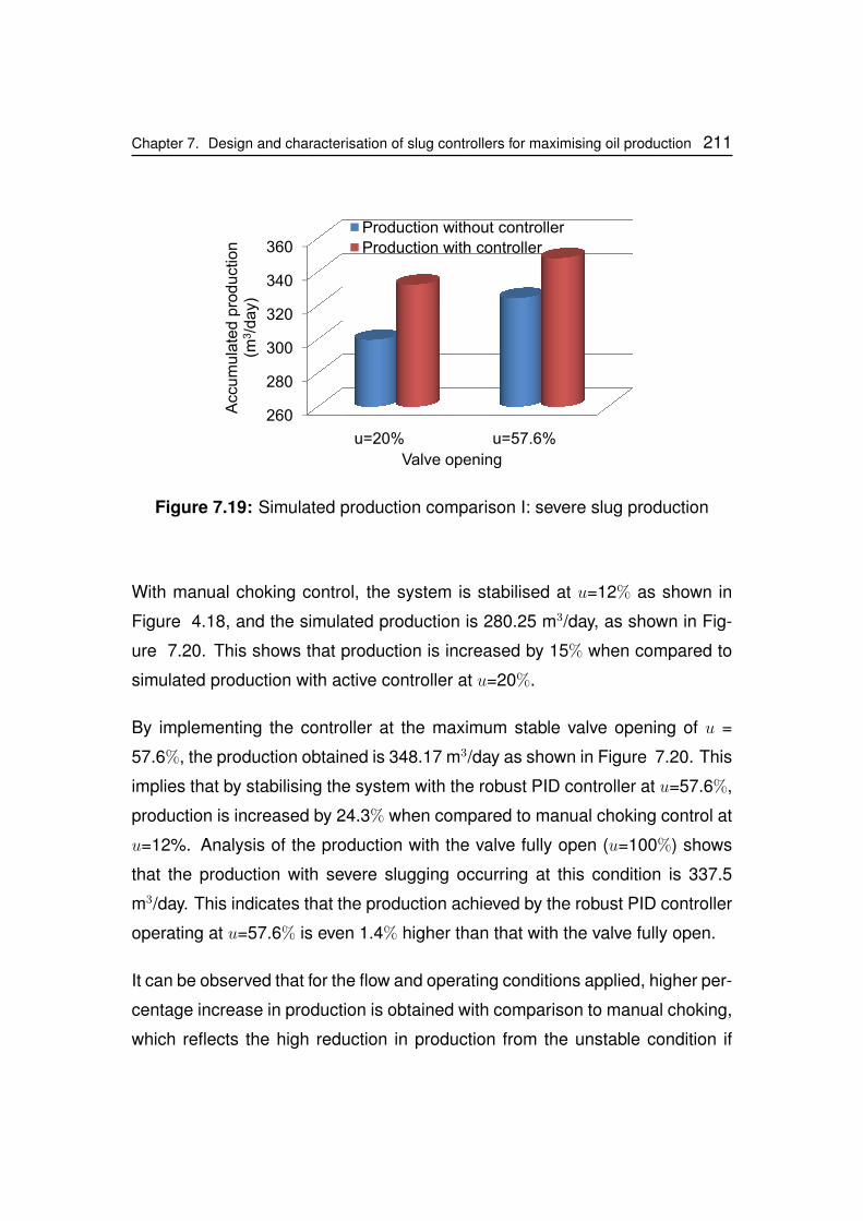
Chapter 7. Design and characterisation of slug controllers for maximising oil production 211
260
280
300
320
340
360A
ccu
mu
late
dp
rod
uctio
n(m
3/d
ay)
u=20% u=57.6%
Valve opening
Production without controller
Production with controller
Production without controller
Figure 7.19: Simulated production comparison I: severe slug production
With manual choking control, the system is stabilised at u=12% as shown in
Figure 4.18, and the simulated production is 280.25 m3/day, as shown in Fig-
ure 7.20. This shows that production is increased by 15% when compared to
simulated production with active controller at u=20%.
By implementing the controller at the maximum stable valve opening of u =
57.6%, the production obtained is 348.17 m3/day as shown in Figure 7.20. This
implies that by stabilising the system with the robust PID controller at u=57.6%,
production is increased by 24.3% when compared to manual choking control at
u=12%. Analysis of the production with the valve fully open (u=100%) shows
that the production with severe slugging occurring at this condition is 337.5
m3/day. This indicates that the production achieved by the robust PID controller
operating at u=57.6% is even 1.4% higher than that with the valve fully open.
It can be observed that for the flow and operating conditions applied, higher per-
centage increase in production is obtained with comparison to manual choking,
which reflects the high reduction in production from the unstable condition if
212 Chapter 7. Design and characterisation of slug controllers for maximising oil production
270
280
290
300
310
320
330
340
350
No controlu=100%
Acc
um
ula
ted
Pro
du
ctio
n(m
3/d
ay)
Different stable and unstable operating points
No controlu=100%
Controlleru=20%
Controlleru=57.6%
Manualchokingu=12%
Different stable and unstable operating points
Production
Manualchokingu=12%
Different stable and unstable operating points
Figure 7.20: Simulated production comparison II: manual choking and no
control
manual choking control method is implemented. Thus, manual choking control
will adversely reduce production, while active slug control at open-loop unsta-
ble operating points will not reduce production, but will under suitable condition
increase production.
7.5.1.3 Implementation of H∞ robust slug controller
The simulation result obtained by implementing the H∞ robust controller de-
signed in section 7.3.3.4 is shown in Figure 7.21. This result indicates that the
controller’s closed-loop stability is limited to minimum PRB of 34.3 barg corre-
sponding to a maximum valve opening of 65.5%. Beyond this point, the input
saturates and the system cannot be stabilised. The comparison of this result
with other controllers’ results is presented in section 7.5.1.4.
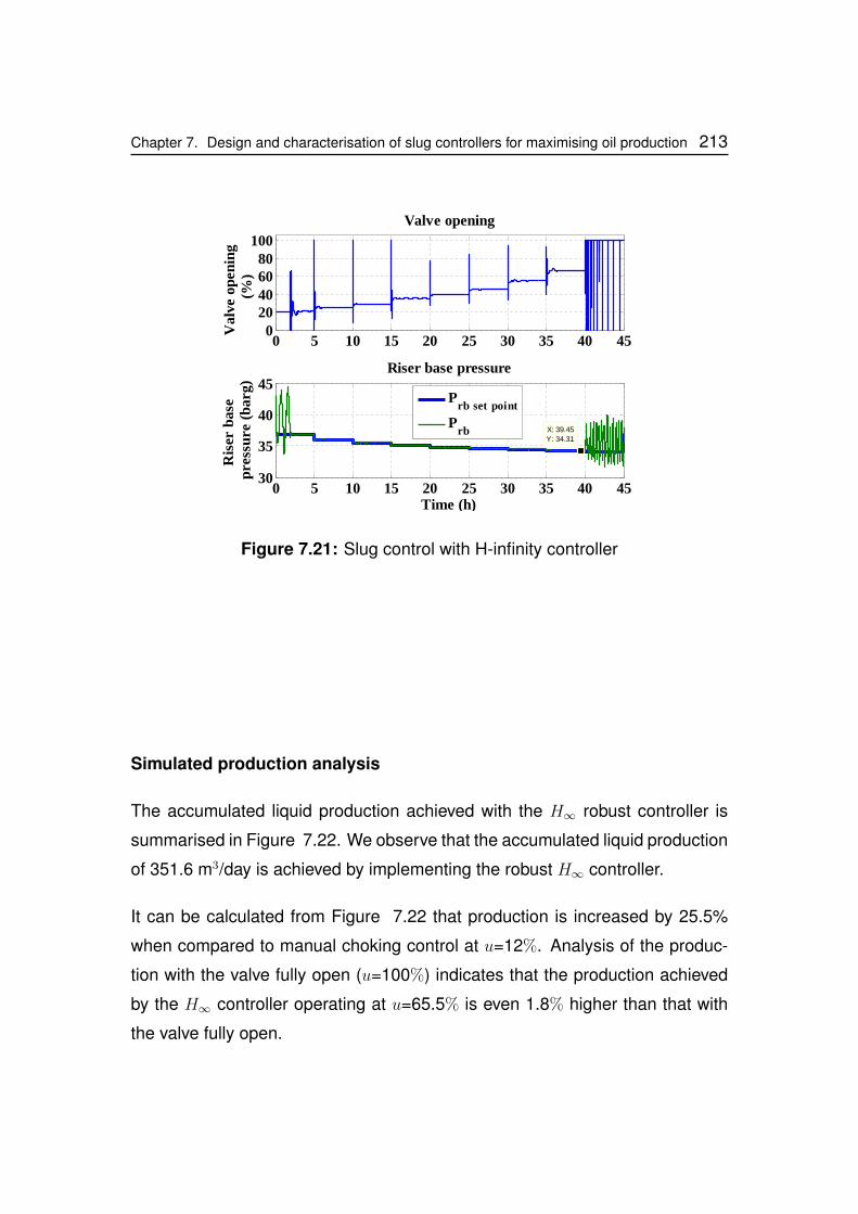
Chapter 7. Design and characterisation of slug controllers for maximising oil production 213
0 5 10 15 20 25 30 35 40 450
20406080
100
Valve openingV
alv
eop
enin
g(%
)
0 5 10 15 20 25 30 35 40 4530
35
40
45
X: 39.45
Y: 34.31
Riser base pressure
Ris
erb
ase
pre
ssu
re(b
arg
)
Time (h)
Prb set point
Prb
Figure 7.21: Slug control with H-infinity controller
Simulated production analysis
The accumulated liquid production achieved with the H∞ robust controller is
summarised in Figure 7.22. We observe that the accumulated liquid production
of 351.6 m3/day is achieved by implementing the robust H∞ controller.
It can be calculated from Figure 7.22 that production is increased by 25.5%
when compared to manual choking control at u=12%. Analysis of the produc-
tion with the valve fully open (u=100%) indicates that the production achieved
by the H∞ controller operating at u=65.5% is even 1.8% higher than that with
the valve fully open.

214 Chapter 7. Design and characterisation of slug controllers for maximising oil production
270
290
310
330
350
370
No controlu=100%
Controlleru=20%
Controlleru=65.5%
Manualchokingu=12%
Accum
ula
ted
liquid
(m3
/da
y)
Different stable and unstable operating points
Production
Figure 7.22: Accumulated oil at different operating points
7.5.1.4 Comparison of maximum stable valve opening and simulated pro-
duction
From Figures 7.15, 7.17 and 7.21 it can be observed that the closed-loop
stable riser system becomes unstable when the valve opening, u, saturates
continuously. The maximum valve opening at which the system become unsta-
ble differs for the three controllers. In section 7.4.1, it was predicted that the
stable closed-loop valve opening, which the H∞ robust controller will achieve
will be larger than that of the relay tuned controller and the robust PID controller,
based on the value of their ‖T‖∞. Comparing the controller performances as
summarised in pressure bifurcation map shown Figure 7.23, it is clear that the
H∞ robust controller achieved closed-loop stability with the least value of PRB,
corresponding to the largest valve opening, when compared to the robust PID
controller and the relay tuned controller. These results are also summarised in
Table 7.12, with the corresponding H∞ shown.
These performances confirms the analysis, that the slug controller with the
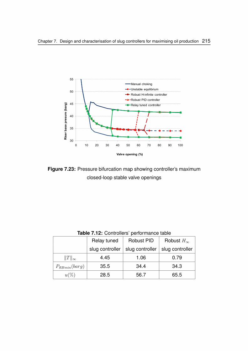
Chapter 7. Design and characterisation of slug controllers for maximising oil production 215
30
35
40
45
50
55
0 10 20 30 40 50 60 70 80 90 100
Manual choking
Unstable equilibrium
Robust H-infinite controller
Robust PID controller
Relay tuned controller
Ris
er
ba
se
pre
su
re(b
arg
)
Valve opening (%)
Figure 7.23: Pressure bifurcation map showing controller’s maximum
closed-loop stable valve openings
Table 7.12: Controllers’ performance tableRelay tuned Robust PID Robust H∞
slug controller slug controller slug controller
‖T‖∞ 4.45 1.06 0.79
PRBmin(barg) 35.5 34.4 34.3
u(%) 28.5 56.7 65.5
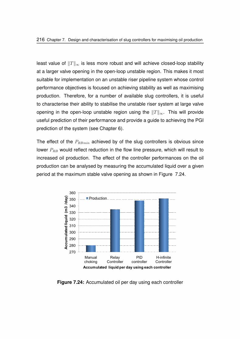
216 Chapter 7. Design and characterisation of slug controllers for maximising oil production
least value of ‖T‖∞ is less more robust and will achieve closed-loop stability
at a larger valve opening in the open-loop unstable region. This makes it most
suitable for implementation on an unstable riser pipeline system whose control
performance objectives is focused on achieving stability as well as maximising
production. Therefore, for a number of available slug controllers, it is useful
to characterise their ability to stabilise the unstable riser system at large valve
opening in the open-loop unstable region using the ‖T‖∞. This will provide
useful prediction of their performance and provide a guide to achieving the PGI
prediction of the system (see Chapter 6).
The effect of the PRBmin achieved by of the slug controllers is obvious since
lower PRB would reflect reduction in the flow line pressure, which will result to
increased oil production. The effect of the controller performances on the oil
production can be analysed by measuring the accumulated liquid over a given
period at the maximum stable valve opening as shown in Figure 7.24.
270
280
290
300
310
320
330
340
350
360
Manualchoking
RelayController
PIDcontroller
H-infiniteController
Ac
cu
mu
late
dli
qu
id(m
3/d
ay
)
Accumulated liquid per day using each controller
Production
Figure 7.24: Accumulated oil per day using each controller
Chapter 7. Design and characterisation of slug controllers for maximising oil production 217
From Figure 7.24, it can be observed that the maximum daily oil production
of 351.6 m3/day is achieved by implementing the robust H∞ controller, while
the minimum daily oil production of 338 m3/day is achieved by the relay tuned
controller. By relating this result to the information shown in Table 7.10 and
Table 7.12, it can be observed that the choice for a stable slug controller for
maximum oil production can be made by analysing the ‖T (s)‖∞ and choosing
the controller with the minimum value. The worst case will be the conventional
and widely used manual choking method, which gives production of 280.25
m3/day resulting to a 25.5% loss in production when compared to production
using robust H∞ controller.
7.5.2 Stability and production in declining reservoir pres-
sure condition
As the well pressure declines (as oil fields mature), the differential pressure
between the topside pressure set point and the well source decreases and the
fluid flow rate is reduced. This would impose further disturbance (instability) on
the riser system such that further action is required to stabilise the system. With
topside valve choking control, this further action would imply reducing the valve
opening further. Implementing manual choking or the robust PID controller in
this condition could have serious impact on production.
Figure 7.25 shows the minimum riser base pressure and the maximum valve
opening required to stabilise the generic (industrial) riser model at declining
reservoir pressure (from 69 barg to 45.3 barg) by using manual choking and
using the open-loop unstable tuned controller. To stabilise the system with
manual choking, the maximum valve opening is reduced from 12% at 69 barg
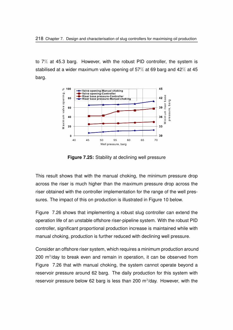
218 Chapter 7. Design and characterisation of slug controllers for maximising oil production
to 7% at 45.3 barg. However, with the robust PID controller, the system is
stabilised at a wider maximum valve opening of 57% at 69 barg and 42% at 45
barg.
Figure 7.25: Stability at declining well pressure
This result shows that with the manual choking, the minimum pressure drop
across the riser is much higher than the maximum pressure drop across the
riser obtained with the controller implementation for the range of the well pres-
sures. The impact of this on production is illustrated in Figure 10 below.
Figure 7.26 shows that implementing a robust slug controller can extend the
operation life of an unstable offshore riser-pipeline system. With the robust PID
controller, significant proportional production increase is maintained while with
manual choking, production is further reduced with declining well pressure.
Consider an offshore riser system, which requires a minimum production around
200 m3/day to break even and remain in operation, it can be observed from
Figure 7.26 that with manual choking, the system cannot operate beyond a
reservoir pressure around 62 barg. The daily production for this system with
reservoir pressure below 62 barg is less than 200 m3/day. However, with the
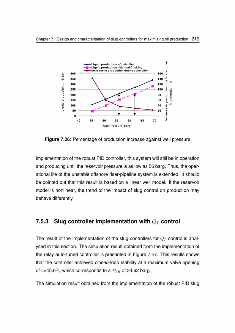
Chapter 7. Design and characterisation of slug controllers for maximising oil production 219
Figure 7.26: Percentage of production increase against well pressure
implementation of the robust PID controller, this system will still be in operation
and producing until the reservoir pressure is as low as 56 barg. Thus, the oper-
ational life of the unstable offshore riser-pipeline system is extended. It should
be pointed out that this result is based on a linear well model. If the reservoir
model is nonlinear, the trend of the impact of slug control on production may
behave differently.
7.5.3 Slug controller implementation with QT control
The result of the implementation of the slug controllers for QT control is anal-
ysed in this section. The simulation result obtained from the implementation of
the relay auto-tuned controller is presented in Figure 7.27. This results shows
that the controller achieved closed-loop stability at a maximum valve opening
of u=45.6%, which corresponds to a PRB of 34.62 barg.
The simulation result obtained from the implementation of the robust PID slug
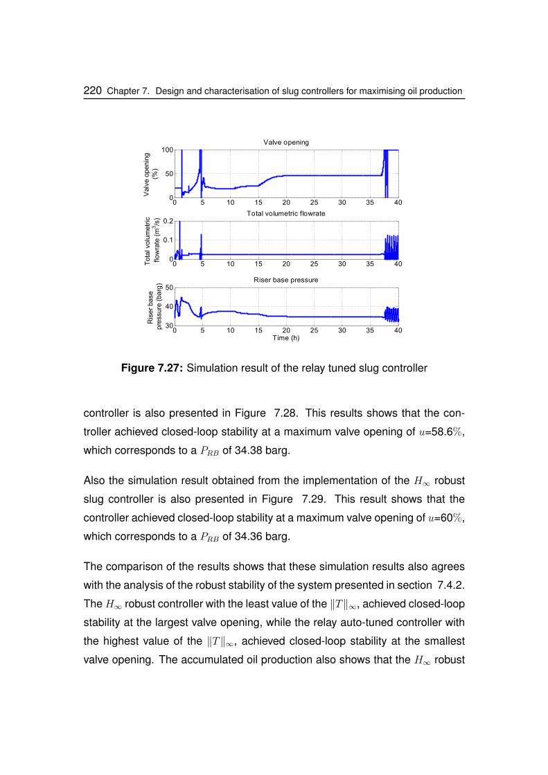
220 Chapter 7. Design and characterisation of slug controllers for maximising oil production
0 5 10 15 20 25 30 35 400
50
100Valve opening
Valv
eopenin
g(%
)
0 5 10 15 20 25 30 35 400
0.1
0.2Total volumetric flowrate
Tota
lvolu
metr
ic
flow
rate
(m3/s
)
0 5 10 15 20 25 30 35 4030
40
50Riser base pressure
Ris
er
base
pre
ssure
(barg
)
Time (h)
Figure 7.27: Simulation result of the relay tuned slug controller
controller is also presented in Figure 7.28. This results shows that the con-
troller achieved closed-loop stability at a maximum valve opening of u=58.6%,
which corresponds to a PRB of 34.38 barg.
Also the simulation result obtained from the implementation of the H∞ robust
slug controller is also presented in Figure 7.29. This result shows that the
controller achieved closed-loop stability at a maximum valve opening of u=60%,
which corresponds to a PRB of 34.36 barg.
The comparison of the results shows that these simulation results also agrees
with the analysis of the robust stability of the system presented in section 7.4.2.
The H∞ robust controller with the least value of the ‖T‖∞, achieved closed-loop
stability at the largest valve opening, while the relay auto-tuned controller with
the highest value of the ‖T‖∞, achieved closed-loop stability at the smallest
valve opening. The accumulated oil production also shows that the H∞ robust
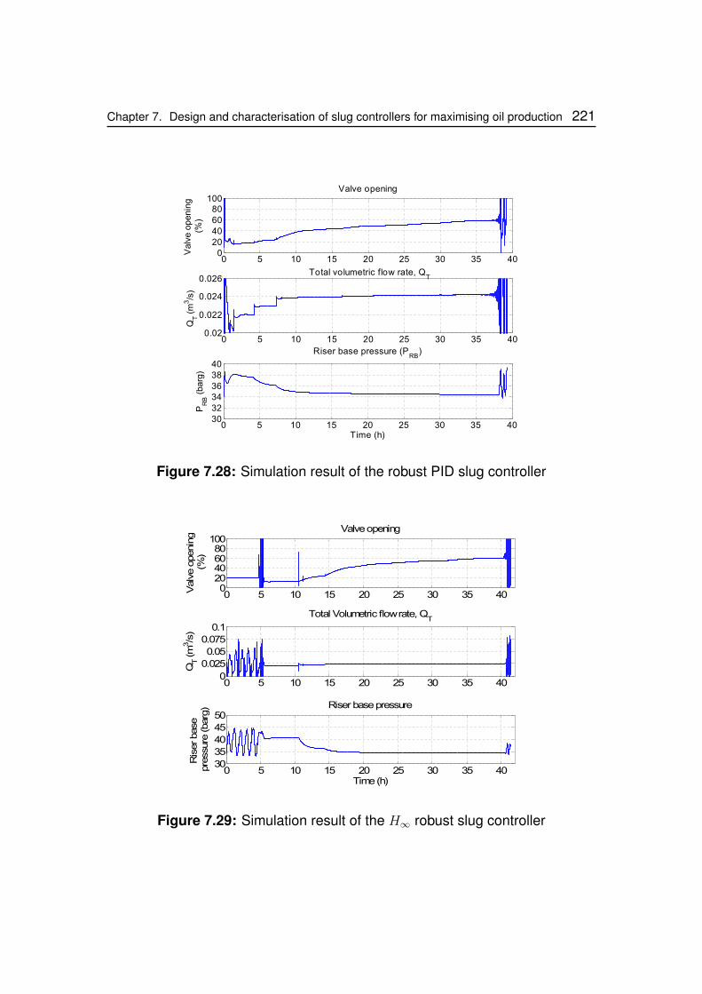
Chapter 7. Design and characterisation of slug controllers for maximising oil production 221
0 5 10 15 20 25 30 35 400
20406080
100Valve opening
Valv
eopenin
g(%
)
0 5 10 15 20 25 30 35 400.02
0.022
0.024
0.026Total volumetric flow rate, Q
T
QT
(m3/s
)
0 5 10 15 20 25 30 35 40303234363840
Riser base pressure (PRB
)
PR
B(b
arg
)
Time (h)
Figure 7.28: Simulation result of the robust PID slug controller
0 5 10 15 20 25 30 35 400
20406080
100Valveopening
Valv
eopenin
g(%
)
0 5 10 15 20 25 30 35 400
0.025
0.05
0.075
0.1
Total Volumetric flowrate, QT
QT
(m3/s
)
0 5 10 15 20 25 30 35 4030
35
40
45
50Riser basepressure
Ris
erbase
pre
ssure
(barg
)
Time(h)
Figure 7.29: Simulation result of the H∞ robust slug controller
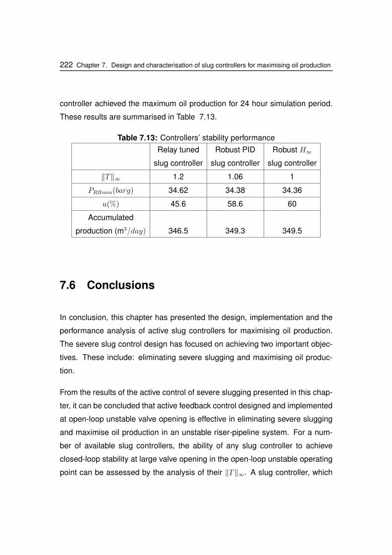
222 Chapter 7. Design and characterisation of slug controllers for maximising oil production
controller achieved the maximum oil production for 24 hour simulation period.
These results are summarised in Table 7.13.
Table 7.13: Controllers’ stability performanceRelay tuned Robust PID Robust H∞
slug controller slug controller slug controller
‖T‖∞ 1.2 1.06 1
PRBmin(barg) 34.62 34.38 34.36
u(%) 45.6 58.6 60
Accumulated
production (m3/day) 346.5 349.3 349.5
7.6 Conclusions
In conclusion, this chapter has presented the design, implementation and the
performance analysis of active slug controllers for maximising oil production.
The severe slug control design has focused on achieving two important objec-
tives. These include: eliminating severe slugging and maximising oil produc-
tion.
From the results of the active control of severe slugging presented in this chap-
ter, it can be concluded that active feedback control designed and implemented
at open-loop unstable valve opening is effective in eliminating severe slugging
and maximise oil production in an unstable riser-pipeline system. For a num-
ber of available slug controllers, the ability of any slug controller to achieve
closed-loop stability at large valve opening in the open-loop unstable operating
point can be assessed by the analysis of their ‖T‖∞. A slug controller, which
Chapter 7. Design and characterisation of slug controllers for maximising oil production 223
achieves the lowest value of the ‖T‖∞, will achieve closed-loop stability at a
larger valve opening than a slug controller with highest ‖T‖∞.
Three active slug controllers namely: the relay auto-tuned controller, the robust
PID controller and the H∞ robust controller has been designed, evaluated and
implemented under the same operating condition for two controlled variables,
the PRB and the QT . The performance evaluation of this set of active slug
controllers has been done by analysing their ‖T‖∞. The analysis revealed that
the H∞ robust controller has the least value of the ‖T‖∞ followed by the robust
PID controller, while the relay auto-tuned controller has the maximum value.
Simulation results obtained from the two controlled variables showed that H∞robust controller achieved closed-loop stability at the maximum valve opening in
the open-loop unstable region, while the relay tuned controller achieved closed-
loop stability at the minimum valve opening.
The maximum liquid production achieved by each controller also differed, re-
flecting the difference in the maximum closed-loop stable valve opening achieved
by each controller. By this, the liquid production achieved by theH∞ robust con-
troller is the maximum for the three controllers.
It was also shown through the analysis of the stability of an unstable offshore
riser system with a declining linear well pressure condition, that the implemen-
tation of a robust slug controller can extend the operational life of such a system.

224 Chapter 7. Design and characterisation of slug controllers for maximising oil production
Chapter 8
Improved relay auto-tuned slug
controller design for increased oil
production
8.1 Introduction
The application of the relay auto-tuned slug controller using the relay shape fac-
tor has some significant advantages, in that it can be applied both online (with
the plant) and offline (through simulation), and its application method does not
require detailed modeling of the system. The plant model can be approximated
from the shape of the relay feedback response as was discussed in Chapter 7.
However, these advantages are undermined by the poor robustness of the slug
controller when it is implemented in the real system. From the performance of
the three slug controllers designed in Chapter 7, it is observed that the relay
auto tuned controller achieved the smallest closed-loop stable operating point
which corresponds to the highest PRB, resulting to the least achieved produc-
tion. This performance reveals the poor robustness of the relay auto tuned slug
225
226 Chapter 8. Improved relay auto-tuned slug controller design for increased oil production
controller. Consequently, the relay tuned controller lacks the ability to handle
plant uncertainties.
Thus, the improvement of the relay auto-tuned slug controller will be necessary
to make it attractive. An approach to achieve this improvement is presented in
this chapter. The chapter begins with the analysis of the perturbed (uncertain)
FOPDT model. This is followed by the development of the improved controller
design algorithm, the controller implementation and the performance analysis.
8.2 The perturbed (uncertain) FOPDT model
By using the shape of the relay feedback response, the riser-pipeline system
model can be identified as the FOPDT process. The process of identifying
this FOPDT process for the riser-pipeline system which had been discussed in
section 7.3.1.1, does not consider the system uncertainties which could affect
the model’s performance in controller design. The model uncertainties occur
due to the difference between the true system and the system model. These
differences often occur due to neglected and unmodeled system dynamics in
the system model [94].
The model uncertainties can be defined with respect to the process parameters
such as the process gain, kp, the process dead time, D, and the process time
constant, τ , which define the model. Consider a nominal (without uncertainty)
unstable FOPDT model of a riser-pipeline system given by:
G0(s) =kpe−Ds
τs− 1(8.1)
Chapter 8. Improved relay auto-tuned slug controller design for increased oil production 227
The model mismatch between the identified FOPDT model and the real system
can be represented in any of these process parameters. We will consider the
pole uncertainty in the identified FOPDT model, since the stability of the system
will depend on its pole location. The pole of (8.1) is 1/τ , which shows that the
pole is a function of the time constant τ . We will define an uncertain time con-
stant of the FOPDT model in (8.1) as τu. With τu, (8.1) will become a perturbed
(uncertain) FOPDT model Gp(s), and can be defined as given in (8.2).
Gp(s) =kpe−Ds
τus− 1(8.2)
The uncertain time constant, τu, can be defined as given in (8.3).
τu = τ(1 + rτ∆) (8.3)
In (8.3), τ is the system’s identified time constant, rτ is the relative magnitude
of the time constant uncertainty and ∆ is the system perturbation, whose mag-
nitude is defined by ‖∆‖∞ < 1. By substituting (8.3) into (8.2), a perturbed
FOPDT model, which is given in (8.4) is obtain.
Gp(s) =kpe−Ds
τs+ rττs∆− 1(8.4)
The term rττs can be defined as a function of an uncertainty weight, wI(s),
such that
rττs = wI(s)(τs− 1) (8.5)
By substituting (8.5) into (8.4), and factorising it, (8.6) is obtained. Equation 8.6
is a perturbed plant with inverse multiplicative uncertainty.
228 Chapter 8. Improved relay auto-tuned slug controller design for increased oil production
Gp(s) =kpe−Ds
(τs− 1)(1 + wI(s)∆)(8.6)
The inverse multiplicative uncertainty is known to be suitable for analysing pole
uncertainty [94]. The uncertainty weight, wI , can be defined by a simple fre-
quency dependent multiplicative weight term. A typical form of this uncertainty
weight which is provided in the literature by Skogestad and Postlethwaite [94],
is given in (8.7).
wI(s) =τ0s+ r0
(τ0/r∞)s+ 1(8.7)
In (8.7), r0 is the relative uncertainty of the system as steady state, 1/τ0 is the
frequency for which the relative uncertainty is 100%, and r∞ is the magnitude
of the weight at high frequency. The wI(s) can be estimated by defining its
parameters to satisfy the condition given in (8.8),
|wI(jω)| ≥ lI(ω),∀ω (8.8)
where lI(ω) is the error between the nominal plant G0(jω) and the perturbed
plant, Gp(jω).
lI(ω) =
∣∣∣∣Gp(jω)−G0(jω)
G0(jω)
∣∣∣∣Having derived the perturbed FOPDT model of the system, the relay auto-tuned
slug controller algorithm is synthesised based on this perturbed FOPDT model
given in (8.6).
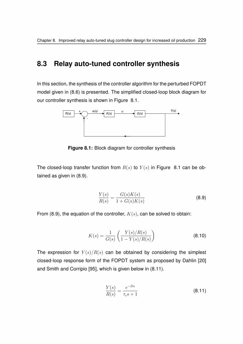
Chapter 8. Improved relay auto-tuned slug controller design for increased oil production 229
8.3 Relay auto-tuned controller synthesis
In this section, the synthesis of the controller algorithm for the perturbed FOPDT
model given in (8.6) is presented. The simplified closed-loop block diagram for
our controller synthesis is shown in Figure 8.1.
e(s)G(s)K(s)
+
-
u Y(s)R(s)
Figure 8.1: Block diagram for controller synthesis
The closed-loop transfer function from R(s) to Y (s) in Figure 8.1 can be ob-
tained as given in (8.9).
Y (s)
R(s)=
G(s)K(s)
1 +G(s)K(s)(8.9)
From (8.9), the equation of the controller, K(s), can be solved to obtain:
K(s) =1
G(s)
(Y (s)/R(s)
1− Y (s)/R(s)
)(8.10)
The expression for Y (s)/R(s) can be obtained by considering the simplest
closed-loop response form of the FOPDT system as proposed by Dahlin [20]
and Smith and Corripio [95], which is given below in (8.11).
Y (s)
R(s)=
e−Ds
τcs+ 1(8.11)
230 Chapter 8. Improved relay auto-tuned slug controller design for increased oil production
where τc is the closed-loop response time constant and D is the dead time of
the identified FOPDT process. By substituting (8.11) into ( 8.10) and simplifying
it, the expression for K(s) is obtained as given in ( 8.12).
K(s) =1
G(s)
(e−Ds
τcs+ 1− e−Ds
)(8.12)
For the purpose of our controller synthesis, the plant model G(s) in (8.12) will
be substituted with the perturbed FOPDT model, Gp(s), given in (8.6). Thus, by
substituting (8.6) into (8.12) and simplifying, the expression for K(s) is obtained
as:
K(s) =(τs+ 1)(1 + wI(s)∆)
kp(τcs+ 1− e−Ds)(8.13)
The delay term, e−Ds, in the denominator can be approximated using the first
order Pade approximation [95], which is given by (8.14).
e−Ds =1− D
2s
1 + D2s
(8.14)
By substituting (8.14) into (8.13), the resulting expression can be simplified to
obtain the algorithm for the PI controller parameters, the controller gain, kc and
the integral time, τI , as given in (8.15) and (8.16)
kc(s) =τ(1 + wI(s)∆)
kp(τc +D)(8.15)
τI = τ(1 + wI(s)∆) (8.16)
Chapter 8. Improved relay auto-tuned slug controller design for increased oil production 231
Equation 8.15, can be further simplified by considering that a closed-loop re-
sponse with 5% overshoot of the set point change is a desired response [95].
For this type of response, it was recommended by Martin et al [65], that the
τc be made equal to the dead time, D, of the FOPDT system. Following this,
(8.15) can be simplified to obtain:
kc(s) =τ(1 + wI(s)∆)
2Dkp(8.17)
For an unstable riser system, at this point, it can be assumed that the model
uncertainty will be dominated by the uncertainty at high frequency. Thus, the
wI(s) in (8.17) can be defined specifically for the uncertainty at high frequency
such that for ω →∞, the uncertainty weight will be equal to the relative uncer-
tainty at high frequency as given in (8.18).
wI(j∞) = r∞ (8.18)
By substituting (8.18) into (8.16) and (8.17), the kc and τI given in 8.19 and 8.20
will obtained.
kc =τ(1 + r∞∆)
2Dkp(8.19)
τI = τ(1 + r∞∆) (8.20)
A systematic method for determining the uncertainty weight parameters will be
explained in the controller design, presented in the next section.
232 Chapter 8. Improved relay auto-tuned slug controller design for increased oil production
8.4 Controller design and implementation
In Chapter 7, the relay auto-tuned slug controller method was implemented
to design slug controllers for PRB and QT control using the riser top valve as
the manipulated variable. The performance of these controllers in achieving
closed-loop stability at large valve opening were not very satisfactory, when
compared to the robust PID and the H∞ robust controller. In this section, the
improved relay design controller algorithm will be implemented to improve the
performance of these controllers on the industrial riser system.
8.4.1 Controller design and implementation with PRB control
The relay auto-tuned controller design for PRB control of the industrial riser
system was carried out in section 7.3.1.4. From the relay feedback response,
the dead time D = 14.2s is obtained and the process gain, kp = 4.72 and time
constant, τ = 20.5 are calculated. Using these parameters, the nominal FOPDT
model G0(s) is defined as given in (8.21).
G0(s) =4.72e−14.2s
20.5s− 1(8.21)
From this nominal plant model, the perturbed plant, Gp(s), is defined as given
in (8.22), by considering the uncertainty of the time constant, τ .
Gp(s) =4.72e−14.2s
τus− 1(8.22)
The range of uncertain time constants, τu, is assume to be ± 90% around the
nominal valve. Using the ureal command in Matlabr Robust Control Toolbox,
a set of 11 samples of the uncertain time constant was obtained. Each sample
Chapter 8. Improved relay auto-tuned slug controller design for increased oil production 233
of τu within the uncertainty set corresponds to a perturbed plant. Thus, based
on (8.22), a set of perturbed plants, Πp, are defined, as given by (8.23).
Πp = {Gp(s, τu)|τu ∈ R+} (8.23)
Given this set of perturbed plant from (8.23), the maximum model error is ob-
tained by evaluating (8.24), for a set of model errors, ΠlI , defined by (8.25),
where lI(i)(ω) is given by (8.26).
lI(ω) = maxGp∈Πp
{ΠlI} (8.24)
ΠlI = {lI(i)(ω)|i ∈ Z+} (8.25)
lI(i)(ω) =
∣∣∣∣Gp(i)(jω)−G0(jω)
G0(jω)
∣∣∣∣ (8.26)
For clarity, the model errors are also plotted in Figure 8.2. The plotted model
errors are obtained by evaluating (8.26), for i = (1, 2, 3, ...n), where n = 11 is
the number of perturbed FOPDT plant in the set Πp.
For the maximum error obtained by evaluating (8.24), it can be observed from
Figure 8.2 that |lI(ω)| is 0.022 at low frequency and 10 at high frequency. With
these values, the uncertainty weight wI(jω) that will account for all the possible
model errors considered, can be designed such that the condition |wI(jω)| ≥|lI(ω)|,∀ω as given in (8.8) is satisfied. Thus, the uncertainty weight is defined
as shown in (8.27), and plotted by the first line in Figure 8.2.
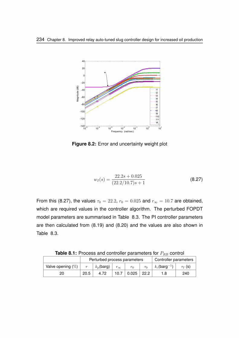
234 Chapter 8. Improved relay auto-tuned slug controller design for increased oil production
10-5
10-4
10-3
10-2
10-1
100
101
-140
-120
-100
-80
-60
-40
-20
0
20
40
Magnitude
(dB
)
Frequency (rad/sec)
l1
l2
l3
l4l5
l6
l7
l8l9
l10
l11
WI
wI
Figure 8.2: Error and uncertainty weight plot
wI(s) =22.2s+ 0.025
(22.2/10.7)s+ 1(8.27)
From this (8.27), the values τ0 = 22.2, r0 = 0.025 and r∞ = 10.7 are obtained,
which are required values in the controller algorithm. The perturbed FOPDT
model parameters are summarised in Table 8.3. The PI controller parameters
are then calculated from (8.19) and (8.20) and the values are also shown in
Table 8.3.
Table 8.1: Process and controller parameters for PRB controlPerturbed process parameters Controller parameters
Valve opening (%) τ kp(barg) r∞ r0 τ0 kc(barg−1) τI (s)
20 20.5 4.72 10.7 0.025 22.2 1.8 240
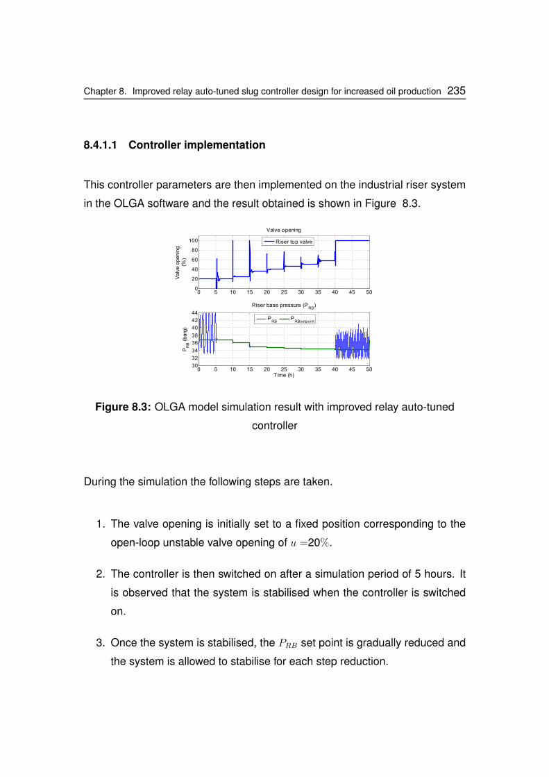
Chapter 8. Improved relay auto-tuned slug controller design for increased oil production 235
8.4.1.1 Controller implementation
This controller parameters are then implemented on the industrial riser system
in the OLGA software and the result obtained is shown in Figure 8.3.
0 5 10 15 20 25 30 35 40 45 500
20
40
60
80
100
Valve opening
Valv
eopenin
g(%
)
Riser top valve
0 5 10 15 20 25 30 35 40 45 5030
32
34
36
38
40
42
44
Riser base pressure (PRB
)
PR
B(b
arg
)
Time (h)
PRB
PRBsetpoint
Figure 8.3: OLGA model simulation result with improved relay auto-tuned
controller
During the simulation the following steps are taken.
1. The valve opening is initially set to a fixed position corresponding to the
open-loop unstable valve opening of u =20%.
2. The controller is then switched on after a simulation period of 5 hours. It
is observed that the system is stabilised when the controller is switched
on.
3. Once the system is stabilised, the PRB set point is gradually reduced and
the system is allowed to stabilise for each step reduction.
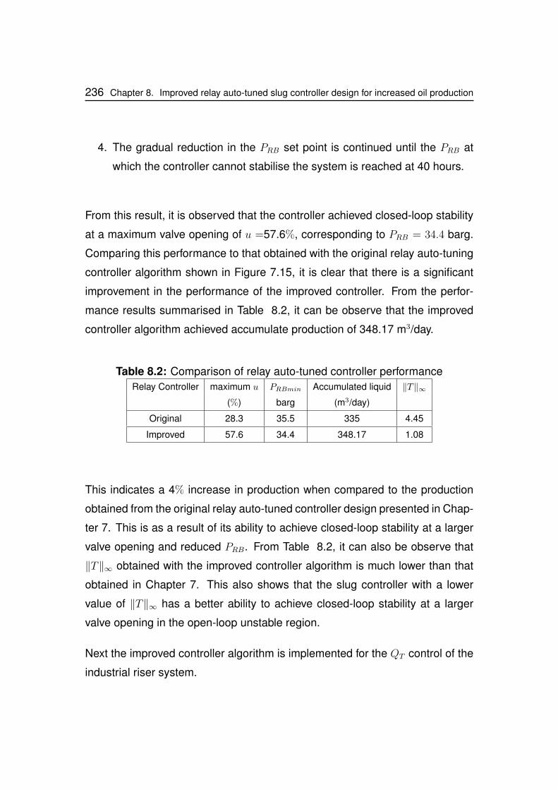
236 Chapter 8. Improved relay auto-tuned slug controller design for increased oil production
4. The gradual reduction in the PRB set point is continued until the PRB at
which the controller cannot stabilise the system is reached at 40 hours.
From this result, it is observed that the controller achieved closed-loop stability
at a maximum valve opening of u =57.6%, corresponding to PRB = 34.4 barg.
Comparing this performance to that obtained with the original relay auto-tuning
controller algorithm shown in Figure 7.15, it is clear that there is a significant
improvement in the performance of the improved controller. From the perfor-
mance results summarised in Table 8.2, it can be observe that the improved
controller algorithm achieved accumulate production of 348.17 m3/day.
Table 8.2: Comparison of relay auto-tuned controller performanceRelay Controller maximum u PRBmin Accumulated liquid ‖T‖∞
(%) barg (m3/day)
Original 28.3 35.5 335 4.45
Improved 57.6 34.4 348.17 1.08
This indicates a 4% increase in production when compared to the production
obtained from the original relay auto-tuned controller design presented in Chap-
ter 7. This is as a result of its ability to achieve closed-loop stability at a larger
valve opening and reduced PRB. From Table 8.2, it can also be observe that
‖T‖∞ obtained with the improved controller algorithm is much lower than that
obtained in Chapter 7. This also shows that the slug controller with a lower
value of ‖T‖∞ has a better ability to achieve closed-loop stability at a larger
valve opening in the open-loop unstable region.
Next the improved controller algorithm is implemented for the QT control of the
industrial riser system.
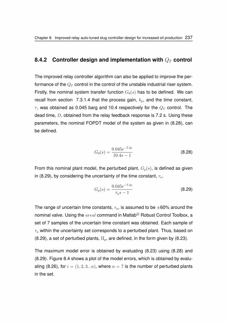
Chapter 8. Improved relay auto-tuned slug controller design for increased oil production 237
8.4.2 Controller design and implementation with QT control
The improved relay controller algorithm can also be applied to improve the per-
formance of the QT control in the control of the unstable industrial riser system.
Firstly, the nominal system transfer function G0(s) has to be defined. We can
recall from section 7.3.1.4 that the process gain, kp, and the time constant,
τ , was obtained as 0.045 barg and 10.4 respectively for the QT control. The
dead time, D, obtained from the relay feedback response is 7.2 s. Using these
parameters, the nominal FOPDT model of the system as given in (8.28), can
be defined.
G0(s) =0.045e−7.2s
10.4s− 1(8.28)
From this nominal plant model, the perturbed plant, Gp(s), is defined as given
in (8.29), by considering the uncertainty of the time constant, τu.
Gp(s) =0.045e−7.2s
τus− 1(8.29)
The range of uncertain time constants, τu, is assumed to be ±60% around the
nominal valve. Using the ureal command in Matlabr Robust Control Toolbox, a
set of 7 samples of the uncertain time constant was obtained. Each sample of
τu within the uncertainty set corresponds to a perturbed plant. Thus, based on
(8.29), a set of perturbed plants, Πp, are defined, in the form given by (8.23).
The maximum model error is obtained by evaluating (8.23) using (8.28) and
(8.29). Figure 8.4 shows a plot of the model errors, which is obtained by evalu-
ating (8.26), for i = (1, 2, 3...n), where n = 7 is the number of perturbed plants
in the set.

238 Chapter 8. Improved relay auto-tuned slug controller design for increased oil production
10-5
10-4
10-3
10-2
10-1
100
101
-140
-120
-100
-80
-60
-40
-20
0
20M
agnitude
(dB
)
Frequency (rad/sec)
l1
l2
l3
l4l5
l6
l7
WI
wI
Figure 8.4: Error and uncertainty weight plot
For the maximum error obtained by evaluating (8.24), it can be observed from
Figure 8.4 that |lI(ω)| is 0.007 at low frequency and and 1.6 at high frequency.
The uncertainty weight parameters will be obtained from this error plot in Fig-
ure 8.4. The uncertainty weight, wI(jω), is then designed such that the con-
dition |wI(jω)| ≥ |lI(ω)|,∀ω is satisfied. The uncertainty weight is as shown in
(8.30), and the uncertainty weight plot is given by the first line from top in Figure
8.4.
wI(s) =8.3s+ 0.008
(8.3/2)s+ 1(8.30)
Table 8.3: Process and the PI controller parameters for QT
Perturbed process parameters Controller parameters
Valve opening (%) τ kp(barg) r∞ r0 τ0 kc(m3/s−1) τI (s)
20 10.5 0.045 2 0.008 8.3 35.6 23
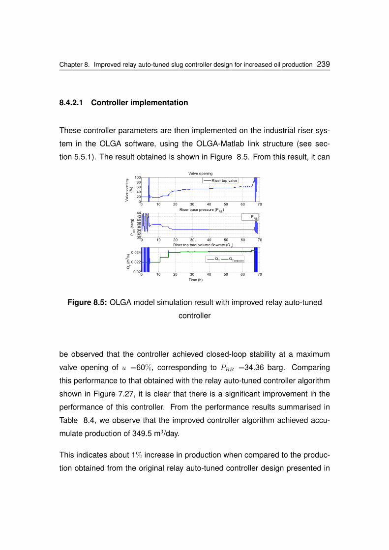
Chapter 8. Improved relay auto-tuned slug controller design for increased oil production 239
8.4.2.1 Controller implementation
These controller parameters are then implemented on the industrial riser sys-
tem in the OLGA software, using the OLGA-Matlab link structure (see sec-
tion 5.5.1). The result obtained is shown in Figure 8.5. From this result, it can
0 10 20 30 40 50 60 700
20
40
60
80
100Valve opening
Valv
eopenin
g(%
)
Riser top valve
0 10 20 30 40 50 60 703032343638404244
Riser base pressure (PRB
)
PR
B(b
arg
)
PRB
0 10 20 30 40 50 60 700.02
0.022
0.024
Riser top total volume flowrate (QT)
QT
(m3/s
)
QT
QTsetpoint
Time (h)
Figure 8.5: OLGA model simulation result with improved relay auto-tuned
controller
be observed that the controller achieved closed-loop stability at a maximum
valve opening of u =60%, corresponding to PRB =34.36 barg. Comparing
this performance to that obtained with the relay auto-tuned controller algorithm
shown in Figure 7.27, it is clear that there is a significant improvement in the
performance of this controller. From the performance results summarised in
Table 8.4, we observe that the improved controller algorithm achieved accu-
mulate production of 349.5 m3/day.
This indicates about 1% increase in production when compared to the produc-
tion obtained from the original relay auto-tuned controller design presented in
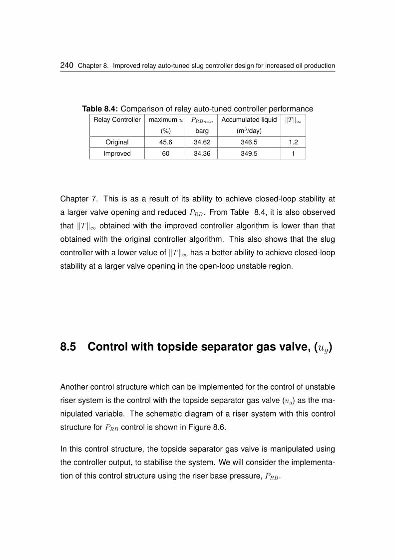
240 Chapter 8. Improved relay auto-tuned slug controller design for increased oil production
Table 8.4: Comparison of relay auto-tuned controller performanceRelay Controller maximum u PRBmin Accumulated liquid ‖T‖∞
(%) barg (m3/day)
Original 45.6 34.62 346.5 1.2
Improved 60 34.36 349.5 1
Chapter 7. This is as a result of its ability to achieve closed-loop stability at
a larger valve opening and reduced PRB. From Table 8.4, it is also observed
that ‖T‖∞ obtained with the improved controller algorithm is lower than that
obtained with the original controller algorithm. This also shows that the slug
controller with a lower value of ‖T‖∞ has a better ability to achieve closed-loop
stability at a larger valve opening in the open-loop unstable region.
8.5 Control with topside separator gas valve, (ug)
Another control structure which can be implemented for the control of unstable
riser system is the control with the topside separator gas valve (ug) as the ma-
nipulated variable. The schematic diagram of a riser system with this control
structure for PRB control is shown in Figure 8.6.
In this control structure, the topside separator gas valve is manipulated using
the controller output, to stabilise the system. We will consider the implementa-
tion of this control structure using the riser base pressure, PRB.
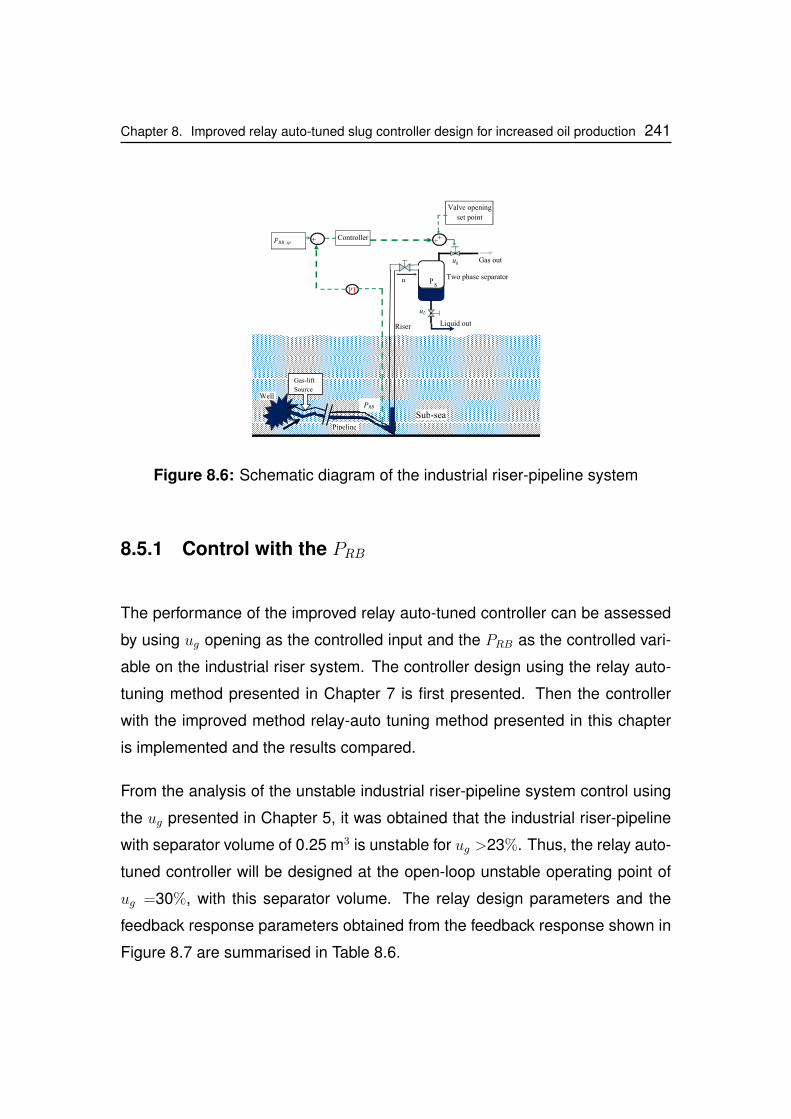
Chapter 8. Improved relay auto-tuned slug controller design for increased oil production 241
PRB
Valve opening
set point
ug
PsTwo phase separator
PT
+ Controller-
u
PRB_sp ++
Riser Liquid out
Gas out
Well
Pipeline
Gas-lift
Source
uL
Sub-sea
Figure 8.6: Schematic diagram of the industrial riser-pipeline system
8.5.1 Control with the PRB
The performance of the improved relay auto-tuned controller can be assessed
by using ug opening as the controlled input and the PRB as the controlled vari-
able on the industrial riser system. The controller design using the relay auto-
tuning method presented in Chapter 7 is first presented. Then the controller
with the improved method relay-auto tuning method presented in this chapter
is implemented and the results compared.
From the analysis of the unstable industrial riser-pipeline system control using
the ug presented in Chapter 5, it was obtained that the industrial riser-pipeline
with separator volume of 0.25 m3 is unstable for ug >23%. Thus, the relay auto-
tuned controller will be designed at the open-loop unstable operating point of
ug =30%, with this separator volume. The relay design parameters and the
feedback response parameters obtained from the feedback response shown in
Figure 8.7 are summarised in Table 8.6.
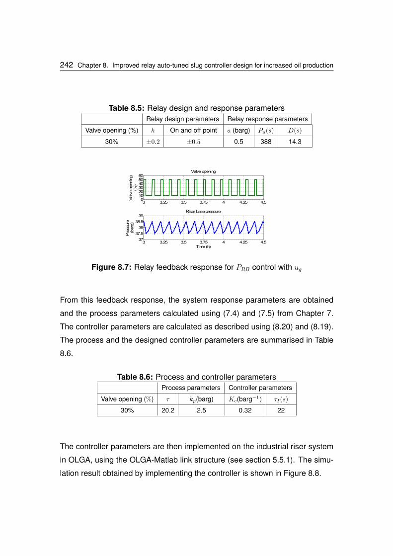
242 Chapter 8. Improved relay auto-tuned slug controller design for increased oil production
Table 8.5: Relay design and response parametersRelay design parameters Relay response parameters
Valve opening (%) h On and off point a (barg) Pu(s) D(s)
30% ±0.2 ±0.5 0.5 388 14.3
3 3.25 3.5 3.75 4 4.25 4.50
102030405060
Valveopening
Valv
eopenin
g(%
)
3 3.25 3.5 3.75 4 4.25 4.537
37.5
38
38.5
39Riser basepressure
Pre
ssu
re(b
arg
)
Time(h)
Figure 8.7: Relay feedback response for PRB control with ug
From this feedback response, the system response parameters are obtained
and the process parameters calculated using (7.4) and (7.5) from Chapter 7.
The controller parameters are calculated as described using (8.20) and (8.19).
The process and the designed controller parameters are summarised in Table
8.6.
Table 8.6: Process and controller parametersProcess parameters Controller parameters
Valve opening (%) τ kp(barg) Kc(barg−1) τI(s)
30% 20.2 2.5 0.32 22
The controller parameters are then implemented on the industrial riser system
in OLGA, using the OLGA-Matlab link structure (see section 5.5.1). The simu-
lation result obtained by implementing the controller is shown in Figure 8.8.
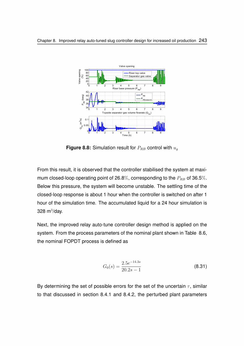
Chapter 8. Improved relay auto-tuned slug controller design for increased oil production 243
0 1 2 3 4 5 6 7 8 90
20406080
100
Valve opening
Valv
eopenin
g(%
)
0 1 2 3 4 5 6 7 8 934
36
38
40
42
Riser base pressure (PRB
)
PR
B(b
arg
)
0 1 2 3 4 5 6 7 8 90
0.05
0.1
Topside separator gas volume flowrate (QGs
)
QG
s(m
3/s
)
Time (h)
PRB
PRBsetpoint
Riser top valve
Separator gas valve
Figure 8.8: Simulation result for PRB control with ug
From this result, it is observed that the controller stabilised the system at maxi-
mum closed-loop operating point of 26.8%, corresponding to the PRB of 36.5%.
Below this pressure, the system will become unstable. The settling time of the
closed-loop response is about 1 hour when the controller is switched on after 1
hour of the simulation time. The accumulated liquid for a 24 hour simulation is
328 m3/day.
Next, the improved relay auto-tune controller design method is applied on the
system. From the process parameters of the nominal plant shown in Table 8.6,
the nominal FOPDT process is defined as
G0(s) =2.5e−14.3s
20.2s− 1(8.31)
By determining the set of possible errors for the set of the uncertain τ , similar
to that discussed in section 8.4.1 and 8.4.2, the perturbed plant parameters
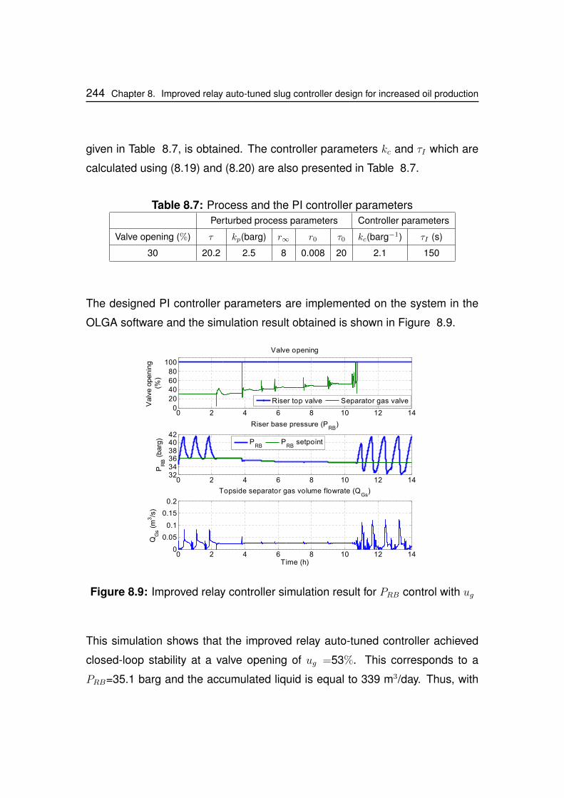
244 Chapter 8. Improved relay auto-tuned slug controller design for increased oil production
given in Table 8.7, is obtained. The controller parameters kc and τI which are
calculated using (8.19) and (8.20) are also presented in Table 8.7.
Table 8.7: Process and the PI controller parametersPerturbed process parameters Controller parameters
Valve opening (%) τ kp(barg) r∞ r0 τ0 kc(barg−1) τI (s)
30 20.2 2.5 8 0.008 20 2.1 150
The designed PI controller parameters are implemented on the system in the
OLGA software and the simulation result obtained is shown in Figure 8.9.
0 2 4 6 8 10 12 140
20
4060
80
100
Valve opening
Valv
eopenin
g(%
)
0 2 4 6 8 10 12 14323436384042
Riser base pressure (PRB
)
PR
B(b
arg
) PRB
PRB
setpoint
0 2 4 6 8 10 12 140
0.05
0.1
0.15
0.2
Topside separator gas volume flowrate (QGs
)
QG
s(m
3/s
)
Time (h)
Riser top valve Separator gas valve
Figure 8.9: Improved relay controller simulation result for PRB control with ug
This simulation shows that the improved relay auto-tuned controller achieved
closed-loop stability at a valve opening of ug =53%. This corresponds to a
PRB=35.1 barg and the accumulated liquid is equal to 339 m3/day. Thus, with

Chapter 8. Improved relay auto-tuned slug controller design for increased oil production 245
the improved controller, a 3.4% increase in production is achieved, when com-
pared with to the production achieved previously. This result clearly shows a
significant improvement when compared to the performance of the original re-
lay tuning method.
8.6 Conclusions
In this chapter, the development, implementation and the performance analysis
of an improved relay auto-tuned slug controller algorithm has been presented.
The developed controller algorithm is based on a perturbed FOPDT model of
the riser system, obtained through relay shape factor analysis.
The developed controller algorithm is implemented on the industrial riser sys-
tem, for PRB control using the riser top valve and the topside separator gas
valve as the manipulated variable. The controller is also implemented for QT
control using the riser top valve as the manipulated variable on the industrial
riser model.
The performance of the improved relay auto-tuned controller showed that the
controllers has the ability to stabilise the unstable riser system at a valve open-
ing that is larger than that achieved with the original (conventional) design algo-
rithm implemented in Chapter 7. About 4% increase in production is achieved
with the improved controller algorithm presented in this chapter, when com-
pared to the the conventional design algorithm implemented in Chapter 7.

246 Chapter 8. Improved relay auto-tuned slug controller design for increased oil production
Chapter 9
Conclusions and further work
9.1 Conclusion
The conclusions from the work presented in this thesis are presented in this
section. This thesis has presented a comprehensive approach to severe slug-
ging control with focus on achieving stable operation and maximising produc-
tion. The body of the thesis contains seven chapters and the conclusions are
drawn from the last six chapters.
A review of the severe slug control techniques, including their applications,
limitations and challenges was presented in Chapter 2. Various forms of se-
vere slug control techniques including modifying internal pipeline diameter, riser
base gas injection, pipeline gas re-injection and manual and active choking of
the riser top vales were discussed. The dearth of sufficient information on the
performance of existing slug control systems is identified as a challenge to de-
ciding the direction for their further development. Also the conflicting report on
the performance of similar techniques exposed the gap in the available knowl-
edge of severe slug control. Extensive amount of work is still required in order
to gain sufficient knowledge and understanding of severe slugging control.
247
248 Chapter 9. Conclusions and further work
The development of the plant-wide model for severe slug control is achieved
with an improved simplified riser model (ISRM) developed to eliminate some
assumptions and limitations of the simplified riser model (SRM) in predicting se-
vere slugging. The model of the two phase separator system and the pressure
dependent well model is developed and linked to the ISRM. Simulation results
from the ISRM shows that it predicts severe slug characteristics, such as pres-
sure amplitude and slug frequency more closely to the experimental result than
the SRM. Also, the ability to predict severe slugging characteristics with chang-
ing inlet flow condition which is not possible with the SRM is achieved with the
ISRM. Improved performance is also achieved with the ISRM in the prediction
of the slug production stage in the severe slug cycle, when compared to the
SRM, against the experimental results. The ability of the ISRM to predict rele-
vant nonlinear stability is investigated using an industrial riser system and a 4
inch laboratory riser system. Its prediction of these nonlinear stabilities showed
close agreement with experimental results.
The controllability analysis of the unstable riser-pipeline system for stability and
production was presented in Chapter 4 to show that by implementing appro-
priate control strategy on the riser-pipeline system, both topside and subsea
variables can be used for stabilising control of the riser pipeline system. The
analysis of the input magnitude required to stabilise the unstable system at the
open-loop unstable valve openings is achieved by evaluating the lower bound
on the transfer function KS. The controllability analysis of an industrial riser
system using the riser top valve, u, as the manipulated variable showed that all
three controlled variables, namely the PRB, the PRT and the QT has the ability
to stabilise the system. However, the controllability analysis showed that gen-
erally, the PRB and the QT has the ability to stabilise the riser system at a larger
valve opening than the PRT . Also the controllability analysis of the system using
the topside separator gas outlet valve, ug, as the manipulated variable showed
Chapter 9. Conclusions and further work 249
that all four variables namely, the PRB, the Ps, the PRT and the QGouts has the
ability to stabilise the system. However, it is shown that generally, the PRB and
the QGouts has the ability to stabilise the riser system at a larger valve open-
ing than the Ps. The difference in their ability to stabilise the system at large
valve opening also revealed their corresponding ability maximise production.
The controllability analysis also showed through simulation that the PRT which
was previously considered to be unsuitable for slug control, and the QT which
is considered to be suitable if it is used in the inner feedback loop in a cascade
control, can be used for slug control if perfect set point tracking of controlled
variable is neglected in the system such that a derivative controller is applied
to stabilise the system at a reference valve opening, with the controller input
equal to the measured value of the controlled variable.
A new concept known as the Production Gain Index (PGI) analysis was in-
troduced in Chapter 5 for systematic analysis of the production potential of a
severe slug control system. The application of the PGI analysis employed a sys-
tematic analysis of the pressure and production relationship in a riser-pipeline
system, using a bifurcation map. The PGI is introduced as the ratio of the
production gain, Jp(u) − Jp(uc) against the pressure dependent production at
steady state Jp(uc). By applying the PGI analysis on an unstable rise-pipeline
system, suitable operating point(s) for maximising production with or without
a slug controller is predicted. Thus, the PGI analysis reveals the potential of a
feedback control system to maximise production in a riser-pipeline system. The
ZPGI contours which is defined as ξ(u, uc) = 0, divides the (u, uc) plane into two
areas; the positive PGI (PPGI) area which is located above the ZPGI line and
the negative PGI (NPGI) area which is located below the ZPGI line. Operating
point on the ZPGI line defined by (u, uc) indicates the valve openings where
the production with a slug controller at uc will be equal to production without
a slug controller (unstable system) at u. In applying a feedback control, any
250 Chapter 9. Conclusions and further work
operating point, (u, uc), located above the ZPGI line corresponds to production
gain operating point known as the PPGI, while any operating point located be-
low the ZPGI line corresponds to a production loss operating point, known as
the NPGI. The implementation of the PGI analysis on an industrial riser system
shows that the prediction of the PGI analysis agrees with the actual simulated
production.
The design of three active slug controllers was presented in Chapter 6 to show
that the ‖T‖∞ can be used to characterise the slug controllers’ ability to achieve
closed loop stability at larger valve opening. The three active slug controllers
include the relay auto-tuned controller, the robust PID controller and the H∞
robust controller. A slug controller which achieved a low value of the ‖T‖∞, will
achieve closed loop stability at a larger valve opening than a slug controller with
high ‖T‖∞. The evaluation of the ‖T‖∞ of these three active slug controllers re-
vealed that the H∞ robust controller has the least value of the ‖T‖∞ followed by
the robust PID controller, while the relay auto-tuned controller has the maximum
value for the two controlled variables considered, namely: the PRB and the QT .
Simulation results obtained from the two controlled variables using an industrial
riser system in OLGA confirmed that the H∞ robust controller achieved closed
loop stability at the maximum valve opening, while the relay tuned controller
achieved closed loop stability at the minimum valve opening. The difference
in the maximum closed loop stable operating point achieved by each controller
also reflected in the liquid production achieved, with the H∞ robust controller
achieving the maximum production among the three controllers.
A new improved relay auto-tuned PI controller algorithm was developed and
implemented in Chapter 7 to improve the performance of the relay tuned slug
controller. The developed controller algorithm is based on a perturbed FOPDT
model of the riser system, obtained through relay shape factor analysis. The
Chapter 9. Conclusions and further work 251
developed controller algorithm is implemented for severe slug control on an in-
dustrial riser system. Its performance indicates that it has the ability to stabilise
the unstable riser system at a valve opening that is larger than that achieved
with the original (conventional) controller algorithm applied, with about 4% in-
crease in production achieved.
9.2 Future work
This work has presented a comprehensive analysis of the systematic approach
to achieving stability and maximising production from an unstable riser-pipeline
system. However, there are still a number of issues which are necessary for
further work, in order to achieve further improvement on this subject.
Currently, the plant-wide model is developed only for severe slugging prediction.
Considering its simplified approach, the model can be extended to predict other
forms of slugging such as the hydrodynamic slugging. Also, the model can be
improved further with focus on modelling the pipeline geometry more accurately
so as to account for the pipeline pressure losses in the model. This can improve
the ability of the model to represent the real system more accurately, and could
improve the performance of the slug controller designed for slug control using
the model.
Since the current plant-wide model can only simulate two phase oil-gas or
water-gas flow, the model can also be further developed to be able to simu-
late three phase oil-water-gas flow. Also, the well model can be extended to
include the nonlinear model
252 Chapter 9. Conclusions and further work
The PGI concept can be further applied on larger and more complex industrial
riser systems under relevant ideal conditions. This will be relevant to improving
the concept and its understanding, and advancing it for industrial application.
The ability of the controlled variables, such as the PRT and Ps to stabilise the
system at larger valve opening can be further improved. There may exist some
control structures or variable combination which could improve the ability of
these variables to stabilise the system at larger valve openings.
The effectiveness of other control design and analysis methods such as struc-
tured singular value and µ-analysis in slug control can be investigated.
The transfer of the knowledge gained in this research for industrial application
can be achieved through the knowledge transfer partnership program.
Appendix A
Simplified riser model (SRM)
equations
The equations of the SRM are presented in this Appendix.
A.1 Conservation equations
Based on the riser-pipeline diagram shown in Figure 4.1, the SRM was devel-
oped with three dynamical states, which account for the:
1. mass of gas in the pipeline, mG1
2. mass of gas at the riser top, mG2
3. mass of liquid in the riser, mL
The corresponding conservation equations are given in (A.1), (A.2) and (A.3).
253
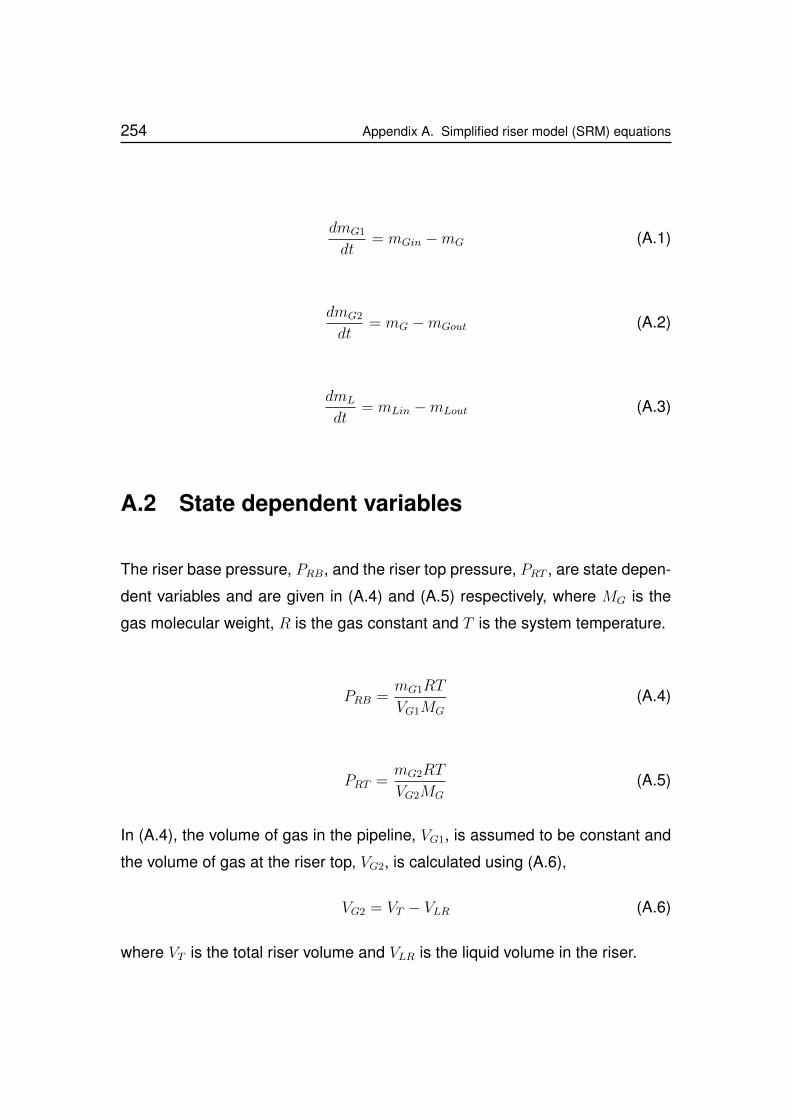
254 Appendix A. Simplified riser model (SRM) equations
dmG1
dt= mGin −mG (A.1)
dmG2
dt= mG −mGout (A.2)
dmL
dt= mLin −mLout (A.3)
A.2 State dependent variables
The riser base pressure, PRB, and the riser top pressure, PRT , are state depen-
dent variables and are given in (A.4) and (A.5) respectively, where MG is the
gas molecular weight, R is the gas constant and T is the system temperature.
PRB =mG1RT
VG1MG
(A.4)
PRT =mG2RT
VG2MG
(A.5)
In (A.4), the volume of gas in the pipeline, VG1, is assumed to be constant and
the volume of gas at the riser top, VG2, is calculated using (A.6),
VG2 = VT − VLR (A.6)
where VT is the total riser volume and VLR is the liquid volume in the riser.
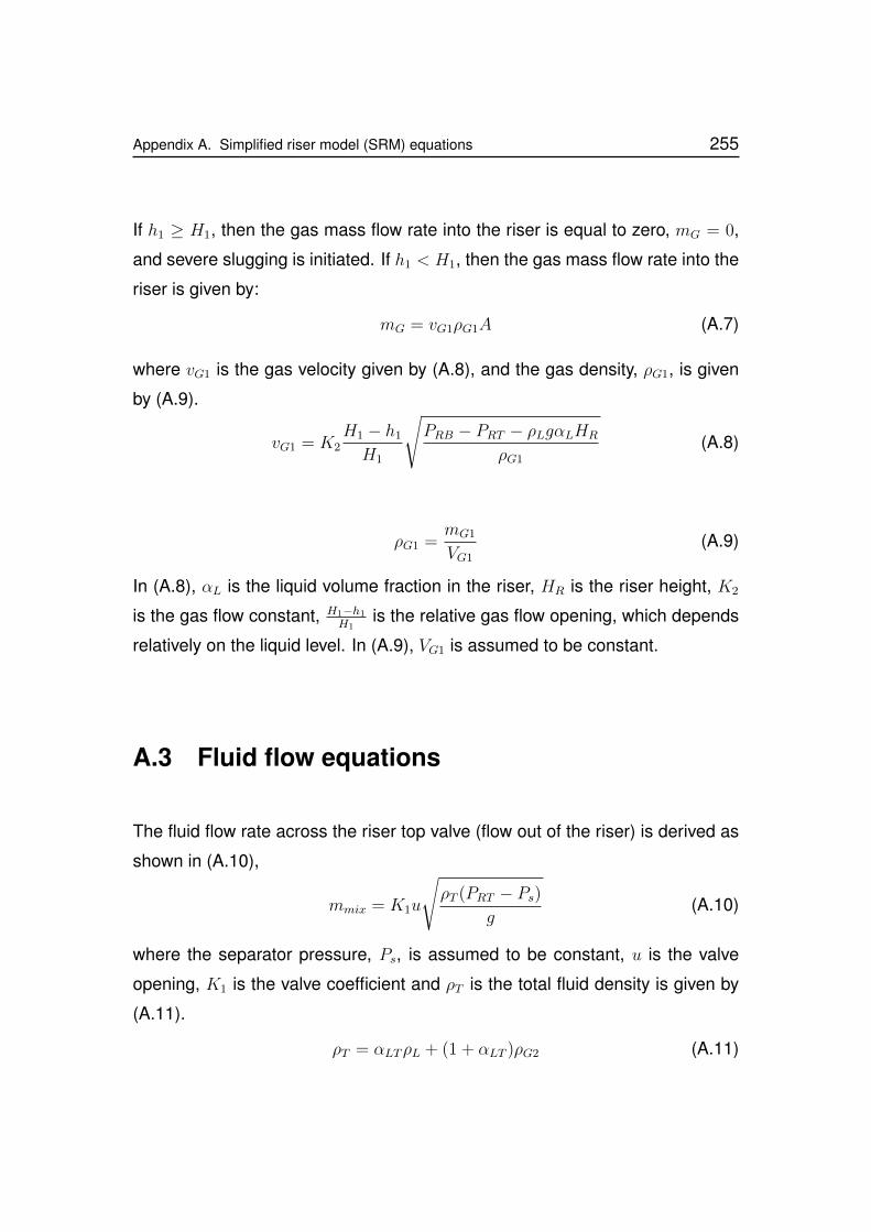
Appendix A. Simplified riser model (SRM) equations 255
If h1 ≥ H1, then the gas mass flow rate into the riser is equal to zero, mG = 0,
and severe slugging is initiated. If h1 < H1, then the gas mass flow rate into the
riser is given by:
mG = vG1ρG1A (A.7)
where vG1 is the gas velocity given by (A.8), and the gas density, ρG1, is given
by (A.9).
vG1 = K2H1 − h1
H1
√PRB − PRT − ρLgαLHR
ρG1
(A.8)
ρG1 =mG1
VG1
(A.9)
In (A.8), αL is the liquid volume fraction in the riser, HR is the riser height, K2
is the gas flow constant, H1−h1H1
is the relative gas flow opening, which depends
relatively on the liquid level. In (A.9), VG1 is assumed to be constant.
A.3 Fluid flow equations
The fluid flow rate across the riser top valve (flow out of the riser) is derived as
shown in (A.10),
mmix = K1u
√ρT (PRT − Ps)
g(A.10)
where the separator pressure, Ps, is assumed to be constant, u is the valve
opening, K1 is the valve coefficient and ρT is the total fluid density is given by
(A.11).
ρT = αLTρL + (1 + αLT )ρG2 (A.11)
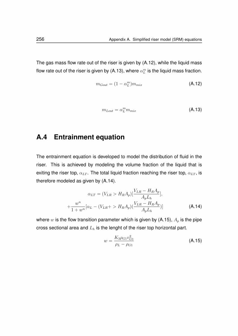
256 Appendix A. Simplified riser model (SRM) equations
The gas mass flow rate out of the riser is given by (A.12), while the liquid mass
flow rate out of the riser is given by (A.13), where αmL is the liquid mass fraction.
mGout = (1− αmL )mmix (A.12)
mLout = αmLmmix (A.13)
A.4 Entrainment equation
The entrainment equation is developed to model the distribution of fluid in the
riser. This is achieved by modeling the volume fraction of the liquid that is
exiting the riser top, αLT . The total liquid fraction reaching the riser top, αLT , is
therefore modeled as given by (A.14).
αLT = (VLR > HRAp)[VLR −HRAp
ApLh],
+wn
1 + wn[αL − (VLR+ > HRAp)(
VLR −HRApApLh
)] (A.14)
where w is the flow transition parameter which is given by (A.15), Ap is the pipe
cross sectional area and Lh is the lenght of the riser top horizontal part.
w =K3ρG1v
2G1
ρL − ρG1
(A.15)

Appendix B
Nonlinear functions for evaluating
system linear transfer functions
B.1 Nonlinear functions for the PRB with u
Equations (B.1) to (B.4) give the nonlinear functions of the transfer function
coefficients against the valve opening for the PRB as the controlled variable. By
evaluating these functions, the linear model transfer function of the system will
be defined at any unstable the steady state valve openings.
f1(ue) = −0.0491u4e + 0.1365u3
e − 0.1303u2e + 0.0393ue − 0.004 (B.1)
f0(ue) = 3× 10⁻⁵u2e + 5× 10⁻⁶ue − 6× 10⁻⁷ (B.2)
g1(ue) = −0.1371u4e + 0.3107u3
e − 0.2101u2e + 0.023ue + 0.034 (B.3)
257
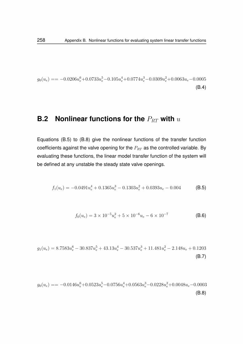
258 Appendix B. Nonlinear functions for evaluating system linear transfer functions
g0(ue) == −0.0206u6e+0.0733u5
e−0.105u4e+0.0774u3
e−0.0309u2e+0.0063ue−0.0005
(B.4)
B.2 Nonlinear functions for the PRT with u
Equations (B.5) to (B.8) give the nonlinear functions of the transfer function
coefficients against the valve opening for the PRT as the controlled variable. By
evaluating these functions, the linear model transfer function of the system will
be defined at any unstable the steady state valve openings.
f1(ue) = −0.0491u4e + 0.1365u3
e − 0.1303u2e + 0.0393ue − 0.004 (B.5)
f0(ue) = 3× 10⁻⁵u2e + 5× 10⁻⁶ue − 6× 10⁻⁷ (B.6)
g1(ue) = 8.7583u6e − 30.837u5
e + 43.13u4e − 30.537u3
e + 11.481u2e − 2.148ue + 0.1203
(B.7)
g0(ue) == −0.0146u6e+0.0523u5
e−0.0756u4e+0.0563u3
e−0.0228u2e+0.0048ue−0.0003
(B.8)
Appendix B. Nonlinear functions for evaluating system linear transfer functions 259
B.3 Nonlinear functions for the QT with u
Equations (B.9) to (B.13) give the nonlinear functions of the transfer function
coefficients against the valve opening for the QT as the controlled variable. By
evaluating these functions, the linear model transfer function of the system will
be defined at any unstable the steady state valve openings.
f1(ue) = −0.0491u4e + 0.1365u3
e − 0.1303u2e + 0.0393ue − 0.004 (B.9)
f0(ue) = 3× 10⁻⁵u2e + 5× 10⁻⁶ue − 6× 10⁻⁷ (B.10)
g2(ue) = −0.454u4e + 1.123u3
e − 0.8458u2e + 0.138ue − 0.122 (B.11)
g1(ue) = −0.0038u4e + 0.0102u3
e − 0.0093u2e + 0.0035ue − 0.0002 (B.12)
g0(ue) = −1× 10⁻⁶u4e + 3× 10⁻⁶u3
e − 3× 10⁻⁶u2e + 1× 10⁻⁶ue− 1× 10⁻⁷ (B.13)
B.4 Nonlinear functions for the PRB with ug
Equation B.14 to B.17 gives the nonlinear functions which define the coeffi-
cients of the open loop transfer function for each operating point for the PRB.
260 Appendix B. Nonlinear functions for evaluating system linear transfer functions
By evaluating these functions, the linear model transfer function of the system
will be defined at any unstable the steady state valve openings.
f1(uge) = 1.5415u5ge−5.0628u4
ge+6.3911u3ge−3.8341u2
ge+1.0633uge−0.1094 (B.14)
f0(uge) = 8× 10⁻⁵u3ge − 0.0002u2
ge + 0.0002uge − 1× 10⁻⁵ (B.15)
g1(uge) = 0.0003u3ge − 0.0011u2
ge + 0.0013uge − 0.0005 (B.16)
g0(uge) = −3×10⁻¹⁵u5ge+2×10⁻¹⁴u4
ge−4×10⁻¹⁴u3ge+3×10⁻¹⁴u2
ge−1×10⁻¹⁴uge+2×10⁻¹⁵
(B.17)
B.5 Nonlinear functions for the Ps with ug
Equation B.18 to B.21 gives the nonlinear functions which define the coeffi-
cients of the open loop transfer function for each operating point for the Ps. By
evaluating these functions, the linear model transfer function of the system will
be defined at any unstable the steady state valve openings.
f1(uge) = 1.5415u5ge−5.0628u4
ge+6.3911u3ge−3.8341u2
ge+1.0633uge−0.1094 (B.18)
Appendix B. Nonlinear functions for evaluating system linear transfer functions 261
f0(uge) = 8× 10⁻⁵u3ge − 0.0002u2
ge + 0.0002uge − 1× 10⁻⁵ (B.19)
g1(uge) = −0.8562u4ge + 2.7509u3
ge − 3.3051u2ge + 1.7697uge (B.20)
g0(uge) = 0.0012u4ge − 0.0041u3
ge + 0.0052u2ge − 0.0029uge + 0.0006 (B.21)
B.6 Nonlinear functions for the PRT with ug
Equation B.22 to B.25 gives the nonlinear functions which define the coeffi-
cients of the open loop transfer function for each operating point for the PRT .
By evaluating these functions, the linear model transfer function of the system
will be defined at any unstable the steady state valve openings.
f1(uge) = 1.5415u5ge−5.0628u4
ge+6.3911u3ge−3.8341u2
ge+1.0633uge−0.1094 (B.22)
f0(uge) = 8× 10⁻⁵u3ge − 0.0002u2
ge + 0.0002uge − 1× 10⁻⁵ (B.23)
g1(uge) = 0.4505u3ge − 1.1103u2
ge + 0.9234uge − 0.2678 (B.24)
g0(uge) = −0.0013u4ge + 0.0024u3
ge − 0.0004u2ge − 0.0012uge + 0.0006 (B.25)

262 Appendix B. Nonlinear functions for evaluating system linear transfer functions
B.7 Nonlinear functions for the QGsep with ug
Equation B.26 to B.29 gives the nonlinear functions which define the coeffi-
cients of the open loop transfer function for each operating point for the QGsep.
By evaluating these functions, the linear model transfer function of the system
will be defined at any unstable the steady state valve openings.
f1(uge) = 1.5415u5ge−5.0628u4
ge+6.3911u3ge−3.8341u2
ge+1.0633uge−0.1094 (B.26)
f0(uge) = 8× 10⁻⁵u3ge − 0.0002u2
ge + 0.0002uge − 1× 10⁻⁵ (B.27)
g1(uge) = −0.2366x3 + 0.6218x2− 0.5445x+ 0.147 (B.28)
g0(uge) = 0.0049u5ge−0.0175u4
ge+0.0242u3ge−0.0165u2
ge+0.0055uge−0.0006 (B.29)
References
[1] AL-KANDARI, A. H., AND KOLESHWAR, V. S. Overcoming slugging prob-
lems in a long-distance multiphase crude pipeline. In Procedings SPE
Annual Technical Conference and Exhibition, Paper SPE 56460 (3-6 Oc-
tober 1999).
[2] AL-SHEIKH, J., SAUNDERS, D., AND BRODKEY, R. Prediction of flow pat-
terns in horizontal two-phase pipe flow. Can. J. of Chemical Engineering
48 (1970), 21–29.
[3] ALVAREZ, C. J., AND AL-MALKI, S. S. Using gas injection for reduc-
ing pressure losses in multiphase pipelines. In Procedings SPE Annual
Technical Conference and Exhibition, Paper SPE 84503 (5-8 October
2003).
[4] ASTROM, K. J., AND HAGGLUND, T. Automatic tuning of simple regula-
tors with specifications on phase and amplitude margins. Automatica 20
(1984), 645–651.
[5] BAKER, O. Simultaneous flow of oil and gas. Oil and Gas Journal 54
(1954), 185–195.
[6] BALINO, J., BURR, K., AND NEMOTO, R. Modeling and simulation of
severe slugging in airwater pipelineriser systems. Int. J. of Multiphase
Flow 36 (2010), 643–660.
263
264 References
[7] BARBUTO, F., AND CAETANO, E. On the occurrence of severe slugging
phenomenon in pargeo-1 platform, campos basin, offshore brazil. Pro-
ceedings 5th International Conference on Multiphase Production, BHRg
(1991), 491–503.
[8] BEGGS, H., AND BRILL, J. A study of two phase flow in inclined pipes. J.
of Petroleum. Technology 25 (1973), 607–617.
[9] BENDIKSEN, K., MALNES, D., AND NULAND, R. M. S. The dynamic
two-fluid model olga: Theory and application. SPE Prod. Eng. 6 (1991),
171–180.
[10] BØE, A. Severe slugging characteristics, part i, flow regime for severe
slugging. Presented at Special Topics in Two-Phase Flow, Trondheim,
Norway (1981).
[11] BONNACAZE, R., ERSKINE, W., AND GRESKOVICH, E. Holdup and pres-
sure drop for two-phase slug flow in inclined pipelines. AIChE J. 17
(1971), 1109–1113.
[12] BOYD, S., GHAOUI, L. E., FREON, E., AND BALAKRISHNAM, V. Linear
matrix inequalities in system and control theory. Society for Industrial and
Applied Mathematics, 3600 University City Science Center, Philadelphia,
Pennsylvania USA (1994).
[13] BRENNEN, C. Fundamentals of Multiphase Flows, 1st edition ed. Cam-
bridge University Press, UK, 2005.
[14] BROWN, M. From chaos to calm. Frontier,
www.bp.com/liveassets/bp internet/globalbp/globalbp uk english/reports
and publications/frontiers/STAGING/local assets/pdf/bpf24 06-
10 slugging.pdf, December 2010.
References 265
[15] CAO, Y., YEUNG, H., AND LAO, L. Inferential slug control system. Report
Report No. 09/YC/533, Cranfield University, Cranfield UK, Department of
Offshore, Process and Energy Engineering, Cranfield University, Cran-
field UK, 2009.
[16] CORNELIUSSEN, S., COUPUT, J.-P., DAHL, E., DYKESTEEN, E.,
FROYSA, K.-E., MALDE, E., MOESTUE, H., MOKSNES, P., SCHEERS,
L., AND TUNHEIM, H. Handbook of multiphase flow metering. Technical
report, Norwegian Society for Oil and Gas Measurement, The Norwegian
Society of Chartered Technical and Scientific Professionals, Solli, OSLO,
March, 2004.
[17] COSTIGAN, G., AND WHALLEY, P. Slug flow regime identification from
dynamic void fraction measurement in vertical air-water flows. Int. J. Mul-
tiphase Flow 23, 2 (1997), 263–283.
[18] COURBOT, A. Prevention of severe slugging in the dunbar 16” multiphase
pipeline. OTC 8196, Offshore Technology Conference (1986), 445–452.
[19] COUSINS, A. R., AND JOHAL, K. S. Multi-purpose riser. European
Patent, No. 00300126.0, Mentor subsea technology services Inc., Hous-
ton Texas (2002).
[20] DAHLIN, E. B. Designing and tuning digital controllers. Instruments and
Control Systems 41, 77 (June, 1968).
[21] DOYLE, J. C. Synthesis of robust controllers and filters. In IEEE Conf.
on Decision and control (San Antonio, Texas, 1983), pp. 109–114.
[22] DOYLE, J. C. Advances in multivariable control. Lecture notes,
ONR/Honeywell Workshop, Minneapolis, USA (October, 1984).
266 References
[23] DRENGSTIG, T., AND MAGNDAL, S. Slug control of production pipeline.
Tech. Rep. N-4091, Stavanger University College, School of Science and
Technology, Ullandhaug, 2001.
[24] DURET, E., AND TRAN, Q. Gas injection controlling liquid slugs in
pipeline riser. UK Patent, No: 02062826 (2002).
[25] ESPEDAL, M., AND BENDIKSEN, K. Onset of instabilities and slugging
in horizontal and near-horizontal gas liquid flow. European Two-Phase
Flow Group Meeting, Paris Paper G4 (May 1989), 1–30.
[26] FABRE, J., PERESSON, L., ODELLO, R., AND ROMANET, T. Severe
slugging in pipeline/riser systems. SPE 16846, Presented at Society of
Petroleum Engineers Annual Technical Conference 19 (1987), 113–129.
[27] FAN, Z., LUSSEYRAN, F., AND HARRANTY, T. Initiation of slugs in hori-
zontal gas-liquid flows. AICHE J. 39 (1993), 1741–1753.
[28] FAN, Z., RUDER, Z., AND HARRANTY, T. Pressure profile for slugs in
horizontal pipes. Int. J. Multiphase Flow 19 (1993), 421–437.
[29] FARGHARLY, M. A. Study of severe slugging in real offshore pipeline
riser-pipe system. In Procedings SPE Middle East Oil Show, Paper SPE
15726 (7-10 March 1997).
[30] FUCHS, P. The pressure limit for terrain slugging. Proceedings 3rd Inter-
national Conference on Multiphase Production, BHRg (1987), 65–71.
[31] GLOVER, K. Robust stabilization of linear multivariable systems: rela-
tions to approximation. Int. J. of Control 43, 3 (1986), 741–766.
[32] GODHAVN, J. M., MEHRDAD, P. F., AND PER, H. F. New slug control
strategy, tuning rules and experimental results. Journal of Process Con-
trol 15, 5 (2005), 547–557.
References 267
[33] GOLDZBERG, V., AND MCKEE, F. Model predicts liquid accumulation,
severe terrain-induced slugging for two phase lines. Oil and Gas Journal
19 (August 1987), 105–109.
[34] GOULD, T., TEK, M., AND KATZ, D. Two-phase flow through vertical,
inclined or curved pipes. J. of Petroleum. Technology 26 (1974), 915–
926.
[35] GOVIER, G., AND OMER, M. The horizontal pipeline flow of air-water
mixtures. Can. J. of Chemical Engineering 40 (1962), 93–104.
[36] GRESKOVICH, E. Holdup prediction for stratified downflow of gas-liquid
mixtures. Ind. Engng Chem., Process Design Development 11 (1972),
81–85.
[37] GROUP, S. P. T. Engineering and operation of production sys-
tem. www.sptgroup.com/upload/documents/Brochures/olga5 dec07.pdf
(April, 2010).
[38] GUET, S., AND OOMS, G. Fluid mechanical aspects of the gas-lift tech-
nique. Annual Review of Fluid Mechanics 38, 1 (2006), 225–249.
[39] HASSANEIN, T., AND FAIRHURST, P. Challenges in the mechanical and
hydraulic aspects of riser design for deep water developments. In Pro-
cedings IBC UK Conf. Ltd. Offshore Pipeline Technology Conference (29
September - 2 October 1998).
[40] HAVRE, K., AND DALSMO, M. Active feedback control as a solution to
severe slugging. In Procedings SPE Annual Technical Conference and
Exhibition, Paper SPE 79252 (2002).
[41] HAVRE, K., STORNES, K., AND STRAY, H. Taming slug flow in pipelines.
Tech. rep., ABB, 2002.
268 References
[42] HENRIOT, V., COURBOT, A., HEINTZ, E., AND MOYEUX, L. Simulation
of process to control severe slugging: application to the dunbar pipeline.
In Procedings SPE Annual Technical Conference and Exhibition, Paper
SPE 56461 (3-6, October 1999).
[43] HILL, T. Multiphase flow field trials on bp’s magnus platform. Journal of
Energy Resources Technology 109 (1987), 142–147.
[44] HILL, T., AND WOOD, D. Slug flow: Occurrence, consequences, and pre-
diction. In Procedings SPE Annual Technical Conference and Exhibition,
Paper SPE 27960 (1994).
[45] HOOGENDOORN, C. Gas liquid flow in horizontal pipes. Chemical Engin-
nering Science 9 (1959), 205–217.
[46] ISHII, M., AND MISHIMA, K. Two-fluid model and hydrodynamic constitu-
tive relations. Nucl. Eng. Des. (1984), 107–126.
[47] ISSA, R., AND KEMPF, M. Simulation of slug flow in horizontal and nearly
horizontal pipes with the two-fluid model. Int. J. Multiphase Flow 29, 1
(2003), 69–95.
[48] ISSA, R., AND WOODBURN, P. Numerical prediction of instabilities and
slug formation in horizontal two-phase flows. 3rd International Confer-
ence on Multiphase Flow, ICMF98, Lyon, France (1998).
[49] JAMAL, H. A., ALI, S. M. F., AND ISLAM, M. R. Petroleum Reservior
Simulation, A Basic Approach, 1st edition ed. Gulf Publishing Company,
Houston TX USA, 2006.
[50] JANSEN, F. E., AND O., S. Method of eliminating pipeline-riser flow insta-
bility. In Procedings SPE Western Regional Meeting, Paper SPE 27867
(23-25, March 1994).
References 269
[51] JANSEN, F. E., SHOHAM, O., AND TAITEL, Y. The elimination of severe
slugging - experiments and modeling. Int. J. of Multiphase Flow 22, 6
(1996), 1055–1071.
[52] JAYANTI, S., AND HEWITT, G. Prediction of the slug-to-churn flow tran-
sition in vertical two-phase flow. Int. J. Multiphase Flow 18, 6 (1992),
847–860.
[53] KADRI, U., ZOETEWEIJ, M., MUDDE, R., AND OLIEMANS, R. A growth
model for dynamic slugs in gasliquid horizontal pipes. Int. J. Multiphase
Flow 35 (2009), 439–449.
[54] KALMAN, R. E. On the general theory of control systems. Proc. 1st
International Congress on Automatic Control 1 (1961), 481–492.
[55] KALMAN, R. E., HO, Y., AND NARENDRA, K. Controllability of linear
dynamic systems. Contrib. Differential Equations 1 (1962), 189–213.
[56] KORDYBAN, E., AND RANOV, T. Mechanism of slug formation in horizon-
tal two-phase flow. J. Bas. Engineering 92 (1970), 857–864.
[57] KOVALEV, K., CRUICKSHANK, A., AND PURVIS, J. The slug suppression
system in operation. In Procedings SPE Annual Technical Conference
and Exhibition, Paper SPE 84947 (2003).
[58] KOVALEV, K., SEELEN, M., AND HAANDRIKMAN, G. Vessel-less s3: Ad-
vanced solution to slugging pipelines. In Procedings SPE Annual Tech-
nical Conference and Exhibition, Paper SPE 88569 (2004).
[59] LARSEN, M., AND HEDNE, P. Three phase slug tracking with petra.
Proceedings 2nd North American Conference on Multiphase Production,
BHRg (2000), 170–192.
270 References
[60] LIN, P., AND HANRATTY, T. Prediction of the initiation of slug with linear
stability theory. Int. J. Multiphase Flow 12 (2003), 79–98.
[61] LINE, A., AND LOPEZ, D. Two-fluid model of wavy seperated two-phase
flow. Int. J. Multiphase Flow 23, 6 (1997), 1131–1146.
[62] LIOMBAS, J., PARAS, S., AND KARABELAS, A. Co-current stratified
gasliquid downflowinfluence of the liquid flow field on interfacial structure.
Int. J. Multiphase Flow 31, 8 (2005), 869–896.
[63] MAKOGAN, T. Y., AND BROOK, G. J. Device for controlling slugging,
world intellectual property organization, 2007/034142 a1, 2007.
[64] MANDHANE, J., GREGORY, G., AND AZIZ, K. A flow pattern map for gas-
liquid flow in horizontal pipes. Int. J. Multiphase Flow 1 (1974), 537–553.
[65] MARTIN, J. J., CORRIPIO, A. B., AND SMITH, C. How to select con-
troller modes and tuning parameters from simple process models. ISA
Transactions 15, 4 (1976), 314–319.
[66] MCQUILLAN1984, K., AND WHALLEY, P. Flow patterns in vertical two-
phase flow. Int. J. Multiphase Flow 11, 2 (1985), 161–175.
[67] MENG, W., AND ZHANG, J. J. Modeling and mitigation of severe riser
slugging: a case study. In Procedings SPE Annual Technical Conference
and Exhibition, Paper SPE 71564 (30 September - 3 October 2001).
[68] MISHIMA, K., AND ISHII, I. Flow regime transition criteria for two-phase
flow in vertical pipes. Int. J. Heat Mass Transfer 27, 5 (1984), 723–737.
[69] MOE, J., LINGELEM, M., HOLM, H., AND OLDERVIK, O. Severe slug-
ging in offshore gas-condensate flowline-riser systems. Proceedings 4th
References 271
International Conference on Multiphase Production, BHRg (1989), 527–
560.
[70] MOKHATAB, S., AND TOWLER, B. Severe slugging in flexible risers: Re-
view of experimental investigations and olga predictions. Petroleum Sci-
ence and Technology 25, 7 (2007), 867–880.
[71] MOLYNEUX, P. D., AND KINVIG, J. P. Method of eliminating severe slug-
ging in a riser of a pipeline includes measuring pipeline pressure and
operating a valve. UK Patent No. 0013331.4., 2000 (2000).
[72] MONTGOMERY, J. Severe slugging and unstable flows in an s-shaped
riser. Ph.d thesis, Cranfield University, Cranfield University, Befordshire,
England, 2002.
[73] MUKHERJEE, H., AND BRILL, J. Emprical equations to predict flow pat-
tern in two-phase inclined flow. Int. J. Multiphase Flow 11, 3 (1985),
299–315.
[74] OGATA, K. Mordern Control Engineering, 4th int. edition ed. Prentice
Hall, Upper Saddle River, New Jersey, 2002.
[75] OGAZI, A. I., CAO, Y., YEUNG, H., AND LAO, L. Robust control of severe
slugging to maximising oil production. In International Conference on
System Engineering (Conventry,UK, 2009), 2009 Conference.
[76] OGAZI, A. I., CAO, Y., YEUNG, H., AND LAO, L. Slug control with large
valve opening to maximising oil production. In SPE Offshore Europe
Conference and Exhibition (Aberdeen ,UK, 2009), Paper SPE 124883.
[77] OGAZI, A. I., OGUNKOLADE, S., CAO, Y., LAO, L., AND YEUNG, H. Se-
vere slugging control through open loop unstable pid tuning to increase
272 References
oil production. In 14th International Conference on Multiphase Technol-
ogy (Cannes, France, June 2009), BHR Group, pp. 17 – 32.
[78] ORAM, P., AND CALVERT, P. Slug mitigation, world intellectual property
organization, wo 2009/133343 a1, 21(3), 5 Nov. 2009.
[79] OZAWA, M., AND SAKAGUCHI, T. Note on modeling of transient slug flow
in multiphase flow system. Memoirs of the Faculty of Engineering, Kobe
University 32 (1985), 25–44.
[80] PANDA, R. C., AND YU, C.-C. Shape factor of relay response curves and
its use in autotuning. Journal of Process Control 15 (2005), 893–906.
[81] PHILIPS, C. L., AND HARBOR, R. D. Feedback Control Systems, 4th
edition ed. Prentice Hall International, Upper Saddle River, New Jersey,
1988.
[82] POTS, B., BROMILOW, I., AND KONIJN, M. Severe slug flow in off-
shore flowline/riser systems. Society of Petroleum Engineers, Middle
East Technical Conference and Exhibition (March 1985), 347–356.
[83] POTS, B. F. M., BROMILOW, I. G., AND KONIJN, M. J. W. F. Severe slug
flow in offshore flow-line/riser systems, spe-13723-pa. SPE Prod. Eng.
2, 4 (1987), 319–324.
[84] ROGER, D. B. Report, Department of Chemistry, The impact of declin-
ing major North Sea oil fields upon Norwegian and United Kingdom oil
production, Northern Kentucky University, Highland Heights, KY 41099-
1905, 2000.
[85] SARICA, C., AND SHOHAM, O. A simplified transient model for pipeline-
riser systems. Chemical Engineering Science 46, 9 (1991), 2167–2179.
References 273
[86] SARICA, C., AND TENGESDAL, J. A new technique to eliminate severe
slugging in pipeline/riser systems. SPE 63185, SPE Annual Technical
Conference and Exhibition, Dallas, TX (2000), 633–641.
[87] SCHICHT, H. Flow patterns for an adiabatic two-phase flow of water and
air within a horizontal tube. Verfahrenstechnik 3, 4 (1969), 153–161.
[88] SCHMIDT, Z., BRILL, J. P., AND BEGGS, H. D. Choking can eliminate
severe pipeline slugging. Oil and Gas Journal 12 (1979), 230–238.
[89] SCHMIDT, Z., BRILL, J. P., AND BEGGS, H. D. Experimental study of
severe slugging in a two-phase-flow pipeline riser pipe system, spe-8306-
pa. SPE Journal 20, 3 (1980), 407–414.
[90] SCHMIDT, Z., DOTY, D. R., AND DUTTA-ROY, K. Severe slugging in
offshore pipeline riser pipe systems. Society of Petroleum Engineers
Journal (1985), 27–38.
[91] SHARMA, Y., IHARA, M., AND MANABE, R. Simulating slug flow in hilly-
terrain pipelines. In SPE Offshore Europe Conference and Exhibition
(Villahermosa, Mexico, 10-12 Feb., 2002), Paper SPE 74359.
[92] SIDI, M. Design of Robust Control Systems, 1st edition ed. Krieger
Publishing Company, Malabar, Florida, 2001.
[93] SINGH, G., AND GRIFFITH, P. Determination of the pressure drop and
optimum pipe size for a two-phase slug flow in an inclined pipe. TRASME,
J. Engng Ind 92 (1970), 717–726.
[94] SKOGESTAD, S., AND POSTLETHWAITE, I. Multivariable Feedback Con-
trol, 2nd edition ed. John Wiley and Sons, UK, 2005.
274 References
[95] SMITH, C. A., AND CORRIPIO, A. B. Principles and Pracice of Automatic
Process Control, 2nd edition ed. John Wiley and Sons, Inc, Canada,
1997.
[96] SPEDDING, P., WOODS, G., RAGHUNATHAN, R., AND WATTERSON, J.
Vertical two-phase flow, part i: Flow regimes. IChemE 76 (July, 1998),
612–629.
[97] STAPLEBERG, H. H., AND MEWES, D. The pressure loss and slug fre-
quency of liquid-liquid-gas flow in horizontal pipes. Int. J. of Multiphase
Flow 20, 2 (April, 1994), 285–303.
[98] STORKAAS, E. Stabilising control and controllability: control solutions to
avoid slug flow in riser-pipeline systems. Thesis, Norwegian University of
Science and Technology, Department of Chemical Engineering, Norwe-
gian University of Science and Technology, 2005.
[99] STORKAAS, E., AND SKOGESTAD, S. Cascade control of unstable sys-
tems with application to stabilization of slug flow. Technical report, De-
partment of Chemical Engineering, Norwegian University of Science and
Technology, Trondheim, Norway (2004).
[100] STORKAAS, E., AND SKOGESTAD, S. Controllability analysis of two-
phase pipeline-riser systems at riser slugging conditions. Control En-
gineering Practice 15, 5 (May, 2007), 567–581.
[101] STORKAAS, E., SKOGESTAD, S., AND ALSTAD, V. Stabilisation of de-
sired flow regimes in pipelines. In AIChE annual meeting (Reno, Nevada,
2001), Paper 287d.
[102] STORKAAS, E., SKOGESTAD, S., AND GODHAVN, J. A low dimensional
dynamic model of severe slugging for control design and analysis. Tech.

References 275
rep., Statoil ASA, R&D, Process Control, Arkitekt Ebells vei 10, Rotvoll,
N-7005, Trondheim, Norway, 2005.
[103] TAITEL, Y. Stability of severe slugging. Int. J. of Multiphase Flow 12, 2
(1986), 203–217.
[104] TAITEL, Y., AND BARNEA, D. Two phase slug flow. Advances in Heat
Transfer, Academic Press (1990), 83–132.
[105] TAITEL, Y., BARNEA, D., AND DUKLER, A. Modelling flow pattern tran-
sition for steady upward gas-liquid flow in vertical tubes. AICHE J. 26
(1980), 345–354.
[106] TAITEL, Y., BARNEA, D., SHOHAM, O., AND DUKLER, A. E. Flow pattern
transition for gas-liquid flow in horizontal and inclined pipes. International
Journal of Multiphase Flow 6 (1979), 217–225.
[107] TAITEL, Y., BARNEA, D., SHOHAM, O., AND DUKLER, A. E. Gas-liquid
flow in inclined tubes: Flow patterns transitions for upward flow. Chemical
Engineering Science 40, 1 (1985), 131–136.
[108] TAITEL, Y., AND DUKLER, A. A model for predicting flow regime transition
in horinzontal and near horizontal gas-liquid flow. AICHE J. 22 (1976),
47–55.
[109] TAITEL, Y., AND DUKLER, A. E. A model for frequency during gas-liquid
flow in horizontal and near horizontal pipes. Int. J. of Multiphase Flow 3,
6 (December, 1977), 585–596.
[110] TENGESDAL, J. O., SARICA, C., AND THOMPSON, L. Severe slugging
attenuation for deepwater multiphase pipeline and riser systems. In Pro-
cedings SPE Annual Technical Conference and Exhibition, Paper SPE
87089 (29 September - 2 October 2002).
276 References
[111] THOMPSON, J. M. T., AND STEWART, H. B. Nonlinear Dynamics and
Chaos, 1st edition ed. John Wiley and Sons Ltd, Chichester Great Britain,
1986.
[112] THYAGARAJAN, T., AND YU, C. C. Improved auto tuning using the shape
factor from relay feedback. Industrial and Engineering Chemistry Re-
search 42, 20 (February 2003), 4425–4440.
[113] UJANG, M. P., LAWRENCE, C. J., HALE, C. P., AND HEWITT, G. F. Slug
initiation and evolution in two-phase horizontal flow. Int. J. Multiphase
Flow 32 (2006), 527–552.
[114] WEISMAN, J. Two-phase Flow Patterns - Chapter 15 in Handbook of
Fluids in Motion, 1st edition ed. Ann Arbor Science Publisher, Michigan,
USA, 1983.
[115] WEISMAN, J., AND KANG, S. Flow pattern transitions in vertical and
upwardly inclined lines. International Journal of Multiphase Flow 7, 27
(1969), 271–291.
[116] YEUNG, H., CAO, Y., AND ADEDIGBA, G. The importance of downstream
conditions on riser behaviour. In 5th North American Conference on Mul-
tiphase Technology (Banff, Canada, June, 2006), 2006 Conference.
[117] ZHENG, G., BRILL, J., AND TAITEL, Y. Slug flow behavior in a hilly terrain
pipeline. Int. J. Multiphase Flow 20 (1994), 63–79.