JHEP09(2013)053

Published for SISSA by Springer

Received: July 29, 2013

Accepted: August 8, 2013

Published: September 10, 2013

Multiloop amplitudes of light-cone gauge bosonic

string field theory in noncritical dimensions

Nobuyuki Ishibashia and Koichi Murakamib

aInstitute of Physics, University of Tsukuba,

Tsukuba, Ibaraki 305-8571, JapanbOkayama Institute for Quantum Physics,

Kyoyama 1-9-1, Kita-ku, Okayama 700-0015, Japan

E-mail: ishibash@het.ph.tsukuba.ac.jp, koichimurakami71@gmail.com

Abstract: We study the multiloop amplitudes of the light-cone gauge closed bosonic

string field theory for d 6= 26. We show that the amplitudes can be recast into a BRST

invariant form by adding a nonstandard worldsheet theory for the longitudinal variables

X± and the reparametrization ghost system. The results obtained in this paper for bosonic

strings provide a first step towards the examination whether the dimensional regularization

works for the multiloop amplitudes of the light-cone gauge superstring field theory.

Keywords: String Field Theory, Conformal Field Models in String Theory, BRST

Symmetry

ArXiv ePrint: 1307.6001

c© SISSA 2013 doi:10.1007/JHEP09(2013)053

JHEP09(2013)053

Contents

1 Introduction 1

2 Amplitudes of light-cone string field theory 2

3 BRST invariant form of the amplitudes 6

3.1 X± CFT 7

3.2 BRST invariant form of amplitudes 9

4 Summary and discussions 10

A Theta functions, prime form and Arakelov Green’s function 11

B Evaluation of ZLC 14

B.1 Integration of the right hand side of eq. (B.1) 15

B.2 Factorization 23

B.2.1 h > 1 case 23

B.2.2 h = 1 case 27

C Modular transformations 31

D A derivation of eq. (3.18) 33

1 Introduction

Light-cone gauge string field theory [1–4] is a formulation of string theory in which the

unitarity of S-matrix is manifest. In the light-cone gauge superstring field theory, regular-

ization is necessary to deal with the contact term problem [5–9]. In refs. [10–15], it has been

proposed to employ dimensional regularization to deal with the divergences in string field

theory. Being a completely gauge fixed formulation, the light-cone gauge NSR string field

theory can be defined in d (d 6= 10) dimensions. By taking d to be a large negative value,

the divergences of the amplitudes are regularized.1 Defining the amplitudes as analytic

functions of d and taking the d → 10 limit, we obtain the amplitudes in critical dimen-

sions. So far, it has been verified that this dimensional regularization scheme works for the

closed string tree-level amplitudes and it has been shown that no divergences occur in the

limit d → 10. This implies that at least at tree level we need not add contact interaction

terms to the string field theory action as counter terms.

1Precisely speaking, in order to deal with the amplitudes involving the strings in the (R,NS) and the

(NS,R) sectors, we shift the Virasoro central charge of the system, rather than the spacetime dimensions

themselves [15]. This can be achieved by adding an extra conformal field theory with sufficiently large

negative central charge.

– 1 –

JHEP09(2013)053

It is obvious that what we should do next is to check whether this regularization scheme

works for the multiloop amplitudes as well. In this paper, as a first step towards this goal,

we study the multiloop amplitudes of the light-cone gauge closed bosonic string field theory

in noncritical dimensions. We evaluate the multiloop amplitudes and give them as inte-

grals over moduli space of the Riemann surfaces corresponding to the Feynman diagrams

for strings. We show that they can be rewritten into a BRST invariant form using the

conformal gauge worldsheet theory. This can be accomplished by adding the longitudinal

variables X± and the ordinary reparametrization bc ghosts in a similar way to the case of

the tree-level amplitudes [11]. The worldsheet theory for the longitudinal variables is the

conformal field theory formulated in ref. [11], which we refer to as the X± CFT.

The organization of this paper is as follows. In section 2, we consider the h-loop

N -string amplitudes for the light-cone gauge closed bosonic string field theory in noncrit-

ical dimensions. Such an amplitude corresponds to a light-cone string diagram which is

conformally equivalent to an N punctured genus h Riemann surface. We present an ex-

pression of the amplitude as an integral over the moduli space of the Riemann surface.

In section 3, the X± CFT on the higher genus Riemann surfaces is constructed. We find

that the prescription developed in the sphere case [11] can be directly generalized to the

present case. Introducing the reparametrization ghost variables as well as the X± CFT,

we rewrite amplitudes into those of the BRST invariant formulation of strings for d 6= 26 in

the conformal gauge. Section 4 is devoted to summary and discussions. In appendix A, the

definitions of the theta functions, the prime form and the Arakelov Green’s functions are

presented. In appendix B, the partition functions of the worldsheet theory on the string di-

agrams are evaluated. In appendix C, we show that the amplitudes of the light-cone gauge

string theory are modular invariant even in noncritical dimensions. In appendix D, we

present a derivation of an identity which is necessary in section 3 to rewrite the amplitudes

into a BRST invariant form.

2 Amplitudes of light-cone string field theory

The light-cone gauge string field theory is defined even for d 6= 26. The action for the

closed string field theory takes a simple form consisting of a kinetic term and a cubic

interaction term:

S =

∫

dt

[

1

2

∫

d1d2 〈R(1, 2)|Φ(t)〉1(

i∂

∂t− L

LC(2)0 + L

LC(2)0 − d−2

12

α2

)

|Φ(t)〉2

+g

6

∫

d1d2d3 〈V3(1, 2, 3)|Φ(t)〉1|Φ(t)〉2|Φ(t)〉3]

. (2.1)

Here |Φ〉r is the string field, dr denotes the integration measure of the momentum zero-

modes given by

dr =αrdαr

4π

dd−2pr(2π)d−2

, (2.2)

αr = 2p+r is the string-length and LLC(r)0 , L

LC(r)0 denote the zero-modes of the transverse

Virasoro generators for the r-th string. The definitions of the reflector 〈R(1, 2)| and the

– 2 –

JHEP09(2013)053

Figure 1. A string diagram with 3 incoming, 2 outgoing strings and 3 loops. The cycles CI going

around the cylinders corresponding to the internal propagators are described. Among them, the

cycle aj is the a cycle for the j-th loop.

three string vertex 〈V3(1, 2, 3)| are presented in appendix A of ref. [11]. Starting from

this action, we can evaluate the amplitudes perturbatively. Each term in the expansion

corresponds to a light-cone gauge Feynman diagram for strings. A typical 3-loop 5-string

diagram is depicted in figure 1.

Mandelstam mapping. A Euclideanized h-loop N -string diagram is conformally equiv-

alent to an N punctured genus h Riemann surface Σ. The light-cone diagram consists of

cylinders. On each cylinder, one can introduce a complex coordinate ρ whose real part

coincides with the Euclideanized light-cone time iX+ and imaginary part parametrizes the

closed string at each time. The ρ’s on the cylinders are smoothly connected except at the

interaction points and we get a complex coordinate ρ on Σ. ρ is not a good coordinate

around the punctures and the interaction points on the light-cone diagram.

ρ can be expressed as an analytic function ρ(z) in terms of a local complex coordinate z

on Σ. As in the tree case, ρ(z) is called the Mandelstam mapping. Let Zr (r = 1, . . . , N) be

the z coordinate of the puncture on Σ which corresponds to the r-th external leg of the light-

cone diagram. The Mandelstam mapping ρ(z) can be determined by the two requirements:

1. The one-form dρ = ∂ρ(z)dz should have simple poles at the punctures Zr with

residues αr and be non-singular everywhere else.2

2. Re ρ has to be globally defined on Σ because it is the light-cone time of the light-

cone string diagram. dρ should therefore have purely imaginary period around any

homology cycle.

These two requirements uniquely fix the one-form dρ [16, 17] and the Mandelstam mapping

ρ(z) is obtained as

ρ(z) =N∑

r=1

αr

[

lnE(z, Zr)− 2πi

∫ z

P0

ω1

ImΩIm

∫ Zr

P0

ω

]

,N∑

r=1

αr = 0 , (2.3)

2To be precise, dρ is a meromorphic one-form on the Riemann surface with N marked points Zr

(r = 1, . . . , N), and holomorphic one-form on the punctured Riemann surface, which has these marked

points removed.

– 3 –

JHEP09(2013)053

up to an additive constant independent of z. Here ω = (ωj) (j = 1, . . . , h) denotes the

canonical basis of the holomorphic one-forms and Ω = (Ωjk) is the period matrix on Σ,

whose definitions are given in appendix A. P0 is an arbitrary point on Σ, which we take

as the base point of the Abel-Jacobi map, and E(z, w) is the prime form [18, 19] defined

in eq. (A.8). Since the one-form dρ has N simple poles, dρ has 2h − 2 + N simple zeros,

which we denote by zI (I = 1, . . . , 2h− 2 +N). They correspond to the interaction points

of the light-cone string diagram.

On the light-cone string diagram, the flat metric

ds2 = dρdρ (2.4)

is chosen as usual, which is referred to as the Mandelstam metric. In terms of a local

coordinate z on Σ, it takes the form

ds2 = |∂ρ(z)|2 dzdz . (2.5)

This metric is singular at the punctures z = Zr and the interaction points z = zI . For

later use, as is done for the tree-level light-cone string diagrams, we introduce the local

coordinate wr around the puncture at z = Zr defined as

wr(z) = exp

[

1

αr(ρ(z)− ρ(zI(r)))

]

, (2.6)

where zI(r) denotes the interaction point on the z-plane where the r-th external string

interacts.

Amplitudes. It is straightforward to calculate the amplitudes by the old-fashioned per-

turbation theory starting from the action (2.1) and Euclideanize the time integrals. An

h-loop N -string amplitude is given as an integral over the moduli space of the string dia-

gram [20] as

A(h)N = (ig)2h−2+NC

∫

[dT ][αdθ][dα]F(h)N , (2.7)

where∫

[dT ][αdθ][dα] denotes the integration over the moduli parameters and C is the

combinatorial factor. In each channel, the integration measure is given as

∫

[dT ][αdθ][dα] =

2h−3+N∏

a=1

(

−i

∫ ∞

0dTa

) h∏

A=1

∫

dαA

4π

3h−3+N∏

I=1

(

|αI |∫ 2π

0

dθI2π

)

. (2.8)

Here Ta’s are heights of the cylinders corresponding to internal lines,3 αA’s denote the

string-lengths corresponding to the + components of the loop momenta and αI ’s and θI ’sare the string-lengths and the twist angles for the internal propagators.

The integrand F(h)N can be described as a correlation function in the light-cone gauge

worldsheet theory for the transverse variables Xi (i = 1, . . . , d− 2). It takes the form [11]

F(h)N = (2π)2δ

(

N∑

r=1

p+r

)

δ

(

N∑

r=1

p−r

)

sgn

(

N∏

r=1

αr

)

(

ZLC)

d−224

⟨

N∏

r=1

V LCr

⟩Xi

. (2.9)

3Heights of the cylinders in a light-cone diagram are constrained so that only 2h − 3 + N of them can

be varied independently.

– 4 –

JHEP09(2013)053

Here V LCr ≡ V LC

r (wr = 0, wr = 0) denotes the light-cone vertex operator for the r-th

external leg located at the origin of the local coordinate wr in eq. (2.6), and⟨

∏Nr=1 V

LCr

⟩Xi

is the expectation value of these operators in the worldsheet theory for the transverse

variables Xi. (ZLC)d−224 denotes the partition function of the worldsheet theory on the

light-cone diagram. The factor sgn(

∏Nr=1 αr

)

comes from the peculiar form of the measure

of αr in eq. (2.2) and our convention for the phase of the vertex 〈V3|. The partition function

ZLC for d = 26 is calculated in appendix B to be

ZLC =1

(32π2)4he−2(h−1)ce2δ(Σ)

∏

r

[

e−2Re Nrr00 (2gA

ZrZr)−1α−2

r

]

∏

I

[

∣

∣∂2ρ(zI)∣

∣

−12gAzI zI

]

.

(2.10)

Here gAzz denotes the Arakelov metric defined in appendix A. The quantities c, δ(Σ) and

N rr00 are defined in eqs. (A.26), (B.44) and (B.18) respectively.

When the r-th external state is of the form

αi1(r)−n1

· · · αı1(r)−n1

· · ·∣

∣p−, pi⟩

r, (2.11)

the vertex operator V LCr becomes

V LCr = αr

∮

0

dwr

2πii∂Xi1(wr)w

−n1r · · ·

∮

0

dwr

2πii∂X ı1(wr)w

−n1r · · ·

× e−p−r τ(r)0 eip

irX

i

(wr = 0, wr = 0) , (2.12)

in which the operators are normal ordered, wr denotes the local coordinate introduced in

eq. (2.6) and τ(r)0 = Re ρ (zI(r)). The on-shell and the level-matching conditions require that

1

2

(

−2p+r p−r + pirp

ir

)

+Nr =d− 2

24, Nr ≡

∑

j

nj =∑

j

nj . (2.13)

We note that the definition of V LCr is independent of the choice of the worldsheet metric to

define the theory and so is the expectation value⟨

∏Nr=1 V

LCr

⟩Xi

. The expectation value⟨

∏Nr=1 V

LCr

⟩Xi

can be expressed in terms of the Green’s functions on Σ. Therefore we can

express the integrand (2.9) in terms of various quantities on Σ defined in appendix A.

Comments. Before closing this section, several comments are in order.

1. Using the Mandelstam mapping, ZLC can be considered as the partition function on

the surface endowed with the Mandelstam metric (2.5) and be written as

ZLC =

(

ZX

[

1

2|∂ρ(z)|2

])24

, (2.14)

where

ZX [gzz] ≡(

8π2 det′gzz∫

dz ∧ dz√g

)− 12

, (2.15)

– 5 –

JHEP09(2013)053

and gzz = −2gzz∂z∂z denotes the scalar Laplacian for conformal gauge metric

ds2 = 2gzzdzdz. From the expression (2.14), we get

ZLC = ZX [gAzz]24e−Γ[gAzz , ln |∂ρ|2] , (2.16)

where Γ[

gAzz, ln |∂ρ|2]

is the Liouville action

Γ[

gAzz, ln |∂ρ|2]

= − 24

48π

∫

dz ∧ dz i(

∂χ∂χ+ gAzzRAχ)

, (2.17)

with χ(z, z) = ln |∂ρ(z)|2 − ln(2gAzz).

In refs. [21, 22], Γ[

gAzz, ln |∂ρ|2]

is calculated by directly evaluating the Liouville

action (2.17). In order to do so, one needs to regularize the divergences coming

from the singularities of the Mandelstam metric (2.5). In ref. [21] a Weyl invariant

but reparametrization noninvariant regularization is employed and e−Γ[gAzz , ln |∂ρ|2] isevaluated to be

e−2(h−1)c∏

r

[

(

2gAZrZr

)−1α2r

]

∏

I

[

∣

∣∂2ρ(zI)∣

∣

−22gAzI zI

]

. (2.18)

Our result for ZLC implies that e−Γ[gAzz , ln |∂ρ|2] is the one given in eq. (B.42), which

includes extra factors of e−2Re Nrr00 and

∣

∣∂2ρ(zI)∣

∣ compared with eq. (2.18). These

factors make Γ[

gAzz, ln |∂ρ|2]

both Weyl and reparametrization invariant as it should

be.4 The regularization employed in ref. [21] does not cause any problems in deriving

the equivalence of the light-cone amplitudes and the covariant ones in the critical

dimensions, but it is not appropriate for the noncritical case.

2. In the light-cone gauge expression (2.7) of the amplitudes, the moduli parameters

T, α, θ are modular invariant, and the integration region covers the moduli space

only once [16]. Being a function of these parameters, the integrand F(h)N should also

be invariant under the modular transformations. However, the explicit form (2.10) of

ZLC and the correlation function⟨

∏Nr=1 V

LCr

⟩Xi

are given in terms of the quantities

such as the theta functions which depend on the choice of the cycles aj , bj . As a

consistency check, it is possible to show that these quantities are invariant under the

modular transformations and do not depend on the choice of these cycles. The details

are given in appendix C.

3 BRST invariant form of the amplitudes

In this section, we would like to rewrite the integrand F(h)N of the amplitudes, given in

eq. (2.9), into the correlation function of the worldsheet theory for strings in the conformal

gauge. By doing so, we will show that there exists a BRST invariant formulation in the

conformal gauge corresponding to the string field theory in the noncritical dimensions. All

these have been done for the tree-level amplitudes in ref. [11].

4It will be possible to get such factors by using the more intricate regularization method in ref. [23].

– 6 –

JHEP09(2013)053

3.1 X± CFT

In order to get the BRST invariant formulation, we need to introduce the longitudinal

variables X± and the reparametrization bc ghosts. The worldsheet theory of X± for d 6= 26

is constructed and called X± CFT [11]. In this subsection, we would like to consider the

X± CFT on the Riemann surface Σ of genus h.

For d = 26, the longitudinal variables X± are introduced in the form of the following

path integral:

∫

[

dX+dX−]gzz

e−S±

d=26

N∏

r=1

e−ip+r X−

(Zr, Zr)M∏

s=1

e−ip−s X+(zs, zs) , (3.1)

where

S±d=26 = − 1

4π

∫

dz ∧ dz i(

∂X+∂X− + ∂X−∂X+)

. (3.2)

Here we take a worldsheet metric ds2 = 2gzzdzdz to define the path integral measure. For

d = 26, we do not have to worry about the choice of gzz.

Since the action for X± is not bounded below, we need to take the integration contour

of X± carefully to define the integral. We decompose the variable X± as

X±(z, z) = X±cl (z, z) + x± + δX±(z, z) , (3.3)

where X±cl (z, z) are solutions to the equations of motion with the source terms5

∂∂X+cl (z, z) = −i

∑

r

p+r (−2πi)δ2(z − Zr) ,

∂∂X−cl (z, z) = −i

∑

s

p−s (−2πi)δ2(z − zs) , (3.4)

and x± + δX±(z, z) are the fluctuations around the solutions with

∫

dz ∧ dz√

gδX± = 0 . (3.5)

The integrals over X± are expressed as those over x± and δX±. In eq. (3.1), we take the

integration contours of x± and δX+−δX− to be along the real axis and that of δX++δX−

to be along the imaginary axis. Then eq. (3.1) becomes well-defined and is evaluated to be

(2π)2δ

(

∑

r

p+r

)

δ

(

∑

s

p−s

)

M∏

s=1

e−ip−s X+cl (zs, zs)Z

X [gzz]2 . (3.6)

Here we can see that the insertion∏N

s=1 e−ip−s X+

(zs, zs) in the path integral (3.1) is replaced

by its classical value∏N

s=1 e−ip−s X+

cl (zs.zs). From eq. (3.4), we can take

X+cl (z, z) = − i

2(ρ (z) + ρ (z)) , (3.7)

5The delta function δ2(z) in eq. (3.4) is normalized so that∫dz ∧ dz δ2(z) = 1.

– 7 –

JHEP09(2013)053

the right hand side of which coincides with the the Lorentzian time of the light-cone string

diagram. As will be explained in the next subsection, one can relate the DDF vertex

operators and the light-cone gauge ones using this fact. Therefore, by considering the

path integral (3.1), one can introduce the longitudinal variables essentially satisfying the

light-cone gauge conditions. Multiplying the path integral for the transverse variables Xi

by the path integral (3.1) for X± and that for the bc ghosts, we are able to get the path

integral for the conformal gauge worldsheet theory.

For d 6= 26, we should specify the metric on the worldsheet to define the path integral.

In the light-cone gauge formulation, the natural choice is

ds2 = −4∂X+∂X+dzdz . (3.8)

This choice is meaningful only when ∂X+∂X+ possesses a reasonable expectation value.

In our case, the expectation value coincides with the Mandelstam metric (2.5). The path

integral measure defined with such a metric can be given as[

dXidX±dbdbdcdc]

−2∂X+∂X+=[

dXidX±dbdbdcdc]

gzze−

d−2624

Γ[gzz , ln(−4∂X+∂X+)] . (3.9)

Thus an extra dependence on the variable X+ comes from the path integral measure.

Including it into the action for X± variables, the action S± becomes

S± [gzz] = − 1

4π

∫

dz ∧ dz i(

∂X+∂X− + ∂X−∂X+)

+d− 26

24Γ[

gzz, ln(

−4∂X+∂X+)]

.

(3.10)

In order to relate the light-cone gauge formulation and the conformal gauge one, we

should consider∫

[

dX+dX−]gzz

e−S±[gzz ]N∏

r=1

e−ip+r X−

(Zr, Zr)M∏

s=1

e−ip−s X+(zs, zs) . (3.11)

This path integral can be evaluated easily as follows. Using the prescription for the contour

of the integration, it is straightforward to prove

0 =

∫

[

dX+dX−]gzz

e−S±

d=26

×N∏

r=1

e−ip+r X−

(Zr.Zr)M∏

s=1

e−ip−s X+(zs.zs)

∏

p

∂δX+(zp)∏

q

∂δX+(zq) . (3.12)

It follows that substituting X+ = X+cl +x++ δX+ into the term Γ

[

gzz, ln(

−4∂X+∂X+)]

of the action S± in eq. (3.11) and expanding it in terms of δX+, we get

⟨

N∏

r=1

e−ip+r X−

(Zr.Zr)M∏

s=1

e−ip−s X+(zs.zs)

⟩X±

gzz

≡ ZX [gzz]−2

∫

[

dX+dX−]gzz

e−S±[gzz ]N∏

r=1

e−ip+r X−

(Zr, Zr)M∏

s=1

e−ip−s X+(zs, zs)

= (2π)2δ

(

∑

s

p−s

)

δ

(

∑

r

p+r

)

∏

s

e−p−sρ+ρ2 (zs, zs) e

− d−2624

Γ[gzz , ln |∂ρ|2] . (3.13)

– 8 –

JHEP09(2013)053

Taking Γ[

gzz, ln |∂ρ|2]

to be the one given in eq. (B.40), it is possible to calculate various

correlation functions of X± from eq. (3.13). One can show that the energy-momentum

tensor of the X± CFT satisfies the Virasoro algebra with the central charge 28 − d [11].

Therefore the worldsheet theory forX±, Xi, b, c, b, c is a CFT with vanishing central charge.

3.2 BRST invariant form of amplitudes

Using eq. (3.13), we find that the product of the light-cone vertex operators V LCr each of

which corresponds to the light-cone state (2.11) is expressed as the expectation value of

that of the DDF vertex operators in the X± CFT:

(2π)2δ

(

N∑

r=1

p+r

)

δ

(

N∑

r=1

p−r

)

N∏

r=1

V LCr (3.14)

=N∏

r=1

(

αre2Re Nrr

00

)

ed−2624

Γ[gzz , ln |∂ρ|2]⟨

N∏

r=1

[

V DDFr (Zr, Zr)e

d−2624

i

p+rX+

(zI(r) , zI(r))

]

⟩X±

gzz

.

Here V DDFr is the DDF vertex operator given by

V DDFr (z, z) = A

i1(r)−n1

(z) · · · Aı1(r)−n1

(z) · · · e−ip+r X−−i

(

p−r −Nr

p+r+ d−26

241

p+r

)

X++ipirXi

(z, z) , (3.15)

with the DDF operator Ai(r)−n for the r-th string defined as

Ai(r)−n (z) =

∮

z

dz′

2πii∂Xi(z′)e

−i n

p+rX+

L (z′), (3.16)

and Aı(r)−n similarly given for the anti-holomorphic sector. The operators in eq. (3.15) are

normal ordered, and X+L (z) in eq. (3.16) denotes the holomorphic part of X+(z, z).

Substituting eq. (3.14) into eq. (2.9) with the worldsheet metric gzz taken to be gAzz,

we find that the integrand F(h)N of the amplitude (2.7) is expressed as

F(h)N ∝

N∏

r=1

(

αre2Re Nrr

00

)

e−Γ[gAzz , ln |∂ρ|2]ZX [gAzz]−2

× ZX [gAzz]d

⟨

N∏

r=1

[

V DDFr (Zr, Zr)e

d−2624

i

p+rX+

(zI(r) , zI(r))

]

⟩Xµ

gAzz

, (3.17)

where 〈· · · 〉Xµ

gzzdenotes the correlation function in the combined system of the worldsheet

theory for Xi (i = 1, . . . , d− 2) and the X± CFT with the metric gzz.

We will further rewrite eq. (3.17) by introducing the ghost variables. It is possible to

show the following identity:

N∏

r=1

(

αre2Re Nrr

00

)

e−Γ[gAzz , ln |∂ρ|2]ZX [gAzz]−2 (3.18)

= const.

∫

[

dbdbdcdc]

gAzz

e−SbcN∏

r=1

cc(Zr, Zr)6h−6+2N∏

K=1

[∫

dz ∧ dz i(

µKb+ µK b)

]

.

– 9 –

JHEP09(2013)053

Here Sbc is the action for the bc ghosts, µK (K = 1, · · · , 6h− 6+ 2N) denote the Beltrami

differentials for the moduli parameters T, α, θ, and const. indicates a constant independent

of the moduli parameters. Eq. (3.18) is derived in appendix D.

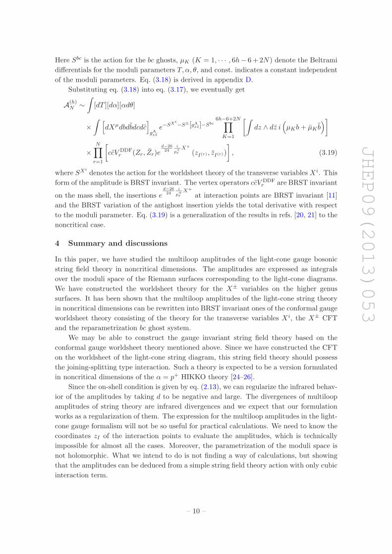
Substituting eq. (3.18) into eq. (3.17), we eventually get

A(h)N ∼

∫

[dT ][dα][αdθ]

×∫

[

dXµdbdbdcdc]

gAzz

e−SXi−S±[gAzz]−Sbc6h−6+2N∏

K=1

[∫

dz ∧ dz i(

µKb+ µK b)

]

×N∏

r=1

[

ccV DDFr (Zr, Zr)e

d−2624

i

p+rX+

(zI(r) , zI(r))

]

, (3.19)

where SXidenotes the action for the worldsheet theory of the transverse variables Xi. This

form of the amplitude is BRST invariant. The vertex operators ccV DDFr are BRST invariant

on the mass shell, the insertions ed−2624

i

p+rX+

at interaction points are BRST invariant [11]

and the BRST variation of the antighost insertion yields the total derivative with respect

to the moduli parameter. Eq. (3.19) is a generalization of the results in refs. [20, 21] to the

noncritical case.

4 Summary and discussions

In this paper, we have studied the multiloop amplitudes of the light-cone gauge bosonic

string field theory in noncritical dimensions. The amplitudes are expressed as integrals

over the moduli space of the Riemann surfaces corresponding to the light-cone diagrams.

We have constructed the worldsheet theory for the X± variables on the higher genus

surfaces. It has been shown that the multiloop amplitudes of the light-cone string theory

in noncritical dimensions can be rewritten into BRST invariant ones of the conformal gauge

worldsheet theory consisting of the theory for the transverse variables Xi, the X± CFT

and the reparametrization bc ghost system.

We may be able to construct the gauge invariant string field theory based on the

conformal gauge worldsheet theory mentioned above. Since we have constructed the CFT

on the worldsheet of the light-cone string diagram, this string field theory should possess

the joining-splitting type interaction. Such a theory is expected to be a version formulated

in noncritical dimensions of the α = p+ HIKKO theory [24–26].

Since the on-shell condition is given by eq. (2.13), we can regularize the infrared behav-

ior of the amplitudes by taking d to be negative and large. The divergences of multiloop

amplitudes of string theory are infrared divergences and we expect that our formulation

works as a regularization of them. The expression for the multiloop amplitudes in the light-

cone gauge formalism will not be so useful for practical calculations. We need to know the

coordinates zI of the interaction points to evaluate the amplitudes, which is technically

impossible for almost all the cases. Moreover, the parametrization of the moduli space is

not holomorphic. What we intend to do is not finding a way of calculations, but showing

that the amplitudes can be deduced from a simple string field theory action with only cubic

interaction term.

– 10 –

JHEP09(2013)053

Bosonic string theory itself is not so interesting anyway, because of the existence of

tachyon. In order to discuss tachyon free theory, we need to supersymmetrize the analyses

in this paper and investigate whether the dimensional regularization scheme proposed in

refs. [10–15] works for the multiloop amplitudes in the light-cone gauge NSR superstring

field theory. Using the supersheet technique [27–30], it will be possible to relate the results

of the light-cone gauge formalism to those of the covariant formalism using the super

Riemann surfaces [31–34].

Acknowledgments

We are grateful to F. Sugino for discussions. N.I. would like to acknowledge the hospitality

of Okayama Institute for Quantum Physics and K.M. would like to thank the hospitality

of Particle Theory Group at University of Tsukuba, where part of this work was done.

This work was supported in part by Grant-in-Aid for Scientific Research (C) (20540247),

(23540332) and (25400242) from MEXT.

A Theta functions, prime form and Arakelov Green’s function

In this appendix, we explain various quantities defined on a genus h Riemann surface Σ,

which are necessary to express the multiloop amplitudes of the light-cone gauge string

field theory.6

In the usual way, we choose on Σ a canonical basis aj , bj (j = 1, . . . , h) of homology

cycles. Let ω = (ωj) = (ω1, . . . , ωh) be the dual basis of holomorphic one-forms on Σ:∮

aj

ωk = δjk ,

∮

bj

ωk = Ωjk , (A.1)

where Ω = (Ωjk) is the period matrix, which is a symmetric h × h complex matrix with

positive definite imaginary part, ImΩ > 0.

Theta functions. With the period matrix Ω in eq. (A.1), any point δ ∈ Ch can be

uniquely expressed in terms of two Rh-vectors as

δ = δ′Ω+ δ′′ , δ′, δ′′ ∈ Rh . (A.2)

The notation [δ] =[

δ′

δ′′

]

is used to represent the point δ ∈ Ch in eq. (A.2). The theta

function with characteristics [δ] =[

δ′

δ′′

]

is defined by

θ[δ](ζ|Ω) =∑

n∈Zh

e2πi[12(n+δ′)Ω(n+δ′)+(n+δ′)(ζ+δ′′)]

= e2πi[12δ′Ωδ′+δ′(ζ+δ′′)] θ(ζ + δ′′ + δ′Ω|Ω) , (A.3)

where θ(ζ|Ω) = θ[0](ζ|Ω). θ[δ](ζ|Ω) is a quasi-periodic function on the Jacobian variety

J(Σ) = Ch/(Zh + Z

hΩ) of the Riemann surface Σ and transforms as

θ[δ](ζ +m+ nΩ|Ω) = e2πimδ′e−2πinδ′′e−πinΩn−2πinζ θ[δ](ζ|Ω) (A.4)

6The mathematical background relevant for string perturbation theory is reviewed in ref. [17].

– 11 –

JHEP09(2013)053

for m,n ∈ Zh. We note that from eq. (A.3) we have

|θ[ζ](0|Ω)| = e−π Im ζ 1ImΩ

Im ζ |θ(ζ|Ω)| . (A.5)

It is immediate from the definition (A.3) that

θ

[

δ′ +m

δ′′ + n

]

(ζ|Ω) = e2πiδ′nθ

[

δ′

δ′′

]

(ζ|Ω) (A.6)

for m,n ∈ Zh. Thus θ[δ] only changes its phase if δ′ and δ′′ are shifted by integral vectors.

The case in which δ′, δ′′ ∈ (Z/(2Z))h is important. In this situation, [δ] =[

δ′

δ′′

]

is referred

to as the spin structure, and we have

θ[δ](−ζ|Ω) = (−1)4δ′δ′′θ[δ](ζ|Ω) . (A.7)

It follows that θ[δ](ζ|Ω) is an even or odd function depending on whether 4δ′δ′′ is an

even or odd integer. [δ] is accordingly referred to as the even spin structure or the odd

spin structure.

Prime form. Let [s] =[

s′

s′′

]

be an odd spin structure. The prime form E(z, w) is de-

fined [18, 19] as

E(z, w) =θ[s]

(∫ z

wω∣

∣Ω)

hs(z)hs(w), (A.8)

where

hs(z) =

√

√

√

√

h∑

j=1

∂θ[s]

∂ζj(0|Ω)ωj(z) (A.9)

is a section of the spin bundle corresponding to [s]. The prime form E(z, w) can be regarded

as a(

−12 , 0)

form in each variable on the universal covering of Σ, whose transformation laws

can be obtained from eq. (A.4) as follows: when z is moved around aj cycle once, E(z, w)

is invariant up to a sign; whereas when z is moved around bj cycle once, it transforms as

E(z, w) 7→ ±e−πiΩjj−2πi∫ zwωjE(z, w) . (A.10)

E(z, w) satisfies E(z, w) = −E(w, z), and for z ∼ w it behaves as

E(z, w) = (z − w) +O(

(z − w)3)

. (A.11)

Arakelov metric and Arakelov Green’s function. Let us define µzz as

µzz ≡1

2hω(z)

1

ImΩω(z) . (A.12)

We note that ∫

Σdz ∧ dz iµzz = 1 , (A.13)

which follows from ∫

Σωj ∧ ωk = −2i ImΩjk . (A.14)

– 12 –

JHEP09(2013)053

The Arakelov metric on Σ,

ds 2A = 2gAzzdzdz , (A.15)

is defined so that its scalar curvature RA ≡ −2gAzz∂∂ ln gAzz satisfies

gAzzRA = −8π(h− 1)µzz . (A.16)

This condition determines gAzz only up to an overall constant, which we will choose later.

The Arakelov Green’s function GA(z, z;w, w) with respect to the Arakelov metric is

defined to satisfy

−∂z∂zGA(z, z;w, w) = −2πiδ2(z − w)− 2πµzz ,

∫

Σdz ∧ dz iµzzG

A(z, z;w, w) = 0 . (A.17)

One can obtain a more explicit form ofGA(z, z;w, w) by solving eq. (A.17) forGA(z, z;w, w).

Using eq. (A.11), we have

∂z∂z lnF (z, z;w, w) = −2πiδ2(z − w)− 2πhµzz , (A.18)

where F (z, z;w, w) is the(

−12 ,−1

2

)

×(

−12 ,−1

2

)

form on Σ× Σ defined as

F (z, z;w, w) = exp

[

−2π Im

∫ z

w

ω1

ImΩIm

∫ z

w

ω

]

|E(z, w)|2 . (A.19)

Putting eqs. (A.18) and (A.16) together, we find that GA(z, z;w, w) is given by

GA(z, z;w, w) = − lnF (z, z;w, w)− 1

2ln(

2gAzz)

− 1

2ln(

2gAww

)

, (A.20)

up to an additive constant independent of z, z and w, w. This possible additive constant

can be absorbed into the ambiguity in the overall constant of gAzz mentioned above. It is

required that eq. (A.20) holds exactly as it is [21, 22, 35]. This implies that

2gAzz = limw→z

exp[

−GA(z, z;w, w)− ln |z − w|2]

, (A.21)

and the overall constant of gAzz is, in principle, determined by the second relation

in eq. (A.17).

Mandelstam mapping. Here we illustrate several properties of the Mandelstam map-

ping (2.3).

The divisor Ddρ =∑2h−2+N

I=1 zI −∑N

r=1 Zr of the one-form dρ satisfies

2h−2+N∑

I=1

∫ zI

P0

ω −N∑

r=1

∫ Zr

P0

ω = 2∆ (mod Zh + Z

hΩ) . (A.22)

Here ∆ is the vector of Riemann constants for P0, which is defined in J(Σ). Its j-th

component ∆j is given by

∆j = −Ωjj

2+

1

2+∑

k 6=j

∮

ak

ωk(P′)∫ P ′

P0

ωj . (A.23)

– 13 –

JHEP09(2013)053

Figure 2. The contours CI .

From the singular behavior of the Mandelstam metric (2.5), one can find that it satisfies

the differential equation

− ∂∂ ln |∂ρ(z)|2 = i2π

(

∑

I

δ2(z − zI)−∑

r

δ2(z − Zr)

)

. (A.24)

This can be solved as

|∂ρ(z)|2 = 2gAzzeχ(z,z) , (A.25)

with

χ(z, z) =N∑

r=1

GA(z;Zr)−2h−2+N∑

I=1

GA(z; zI) + c , (A.26)

where c is a constant independent of z, z but may depend on moduli. We here and hence-

forth suppress the anti-holomorphic coordinate dependence of GA for brevity of notation.

Looking at the behaviors of eq. (A.25) around z ∼ zI and z ∼ Zr, one finds that

∣

∣∂2ρ(zI)∣

∣

2=(

2gAzI zI)2

exp

−∑

J 6=I

GA(zI ; zJ) +∑

r

GA(zI ;Zr) + c

,

|αr|2 = exp

−∑

I

GA(zI ;Zr) +∑

s 6=r

GA(Zr;Zs) + c

, (A.27)

and thus

∏

I

∣

∣∂2ρ(zI)∣

∣

2= e(2h−2+N)c

∏

I

(

2gAzI zI)2

exp

−2∑

I<J

GA(zI ; zJ) +∑

I,r

GA(zI ;Zr)

,

∏

r

|αr|2 = eNc exp

−∑

I,r

GA(zI ;Zr) + 2∑

r<s

GA(Zr;Zs)

. (A.28)

B Evaluation of ZLC

In this appendix, we will evaluate the partition function (ZLC)d−224 for the transverse coor-

dinates Xi. In the following, we consider the case d = 26 to get the partition function ZLC.

ZLC can be obtained by integrating the change δ lnZLC under the variation of moduli

parameters, as in the tree case [11]. Since ZLC is the partition function, if we vary the

– 14 –

JHEP09(2013)053

Figure 3. The cycles corresponding to the variations of the + components of the loop momenta.

lengths and the twist angles of the internal propagators of the light-cone diagram, the

change of ZLC is given in terms of the expectation values of the Hamiltonian and the

rotation generator as

δ lnZLC =∑

IδTI

∮

CI

dρ

2πi

⟨

T trρρ

⟩Xi

+ c.c. . (B.1)

Here I labels the internal lines of the light-cone diagram Σ and CI denotes the contour

going around it as depicted in figure 2. TI is defined as

TI = TI + iαIθI , (B.2)

where TI denotes the length of the I-th internal line and αI , θI denote the string-length

and the twist angle for the propagator. Re δTI ’s should satisfy some linear constraints so

that the variation corresponds to that of the shape of a light-cone diagram.⟨

T trρρ

⟩Xi

denotes

the expectation value of the energy-momentum tensor T trρρ on the light-cone diagram for the

worldsheet bosons Xi(i=1, . . . , 24) corresponding to the transverse spacetime coordinates.

What we would like to do in the following is to calculate the right hand side of eq. (B.1)

and integrate it. The variation we consider here corresponds to that of only a subset of

6h−6+2N moduli parameters. We do not consider the variation of αI ’s which are not fixed

by the momentum conservation, namely that of the + components of the loop momenta.

Such variations correspond to integration cycles depicted in figure 3. Therefore integrating

the right hand side of eq. (B.1), integration constants depending on these parameters are

left undetermined. We will fix these imposing the factorization conditions in subsection B.2.

B.1 Integration of the right hand side of eq. (B.1)

In order to integrate the right hand side of eq. (B.1), we introduce a convenient way to

parametrize the moduli of the surface. As is depicted in figure 4, cutting along h cycles

with constant Re ρ, one can make Σ into a surface with no handles but with 2h holes.

By attaching 2h semi-infinite cylinders to the holes, it is possible to get a tree light-cone

diagram, which is denoted by Σ. Let ρ (z) be the Mandelstam mapping which maps

C ∪ ∞ to Σ:

ρ : C ∪ ∞ −→ Σ

z 7→ ρ (z) . (B.3)

ρ (z) has the form

ρ (z) =N∑

r=1

αr ln (z − Zr) +h∑

A=1

βA lnz −QA

z −RA. (B.4)

– 15 –

JHEP09(2013)053

Figure 4. The h cycles along which we cut the light-cone diagram to make the Riemann surface

Σ corresponding to the light-cone diagram into a surface with no handles but with 2h holes.

Here βA (A = 1, · · · , h) are real positive parameters corresponding to the lengths of the h

cycles along which the surface Σ is cut. The surface Σ can be obtained from Σ by discarding

the 2h semi-infinite cylinders and identifying the boundaries. Therefore we can use the z

coordinate to describe Σ and we do so in the rest of this subsection. The Mandelstam

mapping ρ(z) can be given as

ρ(z) = ρ(z) + (purely imaginary constant) , (B.5)

and Σ corresponds to C∪∞ with disks DQA, DRA

(A = 1, · · · , h) around QA, RA excised.

We identify z ∈ ∂DQAand w ∈ ∂DRA

if

ρ (z) = ρ (w) + iβA(θA + 2πn) , (B.6)

for n ∈ Z.

From the construction above, one can see that it is possible to associate the parameters

Zr, βA, θA, QA, RA with any light-cone diagram. Therefore, with αr (= 2p+r ) fixed, the

shape of Σ is parametrized locally by Zr, βA, θA, QA, RA modded out by the 6 conformal

transformations on C ∪ ∞. Thus we have 2N + h + h + 2h + 2h − 6 = 6h − 6 + 2N

real parameters, the number of which coincides with that of the moduli parameters of the

punctured Riemann surface Σ. A variation of the complex structure of Σ corresponds to

a variation of these parameters. βA’s correspond to the loop momenta and the variation

we consider here corresponds to the one with δβA = 0. Under such a variation of the

parameters, the rule of identification (B.6) is also changed as

(ρ+ δρ) (z) = (ρ+ δρ) (w + δw) + iβA(θA + δθA + 2πn) . (B.7)

Accordingly we obtain

δρ (z)− δρ (w) = δw∂ρ (w) + iβAδθA . (B.8)

Therefore as a function on Σ, the variation δρ (z) is discontinuous along the cycle corre-

sponding to ∂DQA.

In terms of the quantities defined using the z coordinate, the right hand side of eq. (B.1)

can be expressed as

δ lnZLC =∑

IδTI

∮

CI

dz

2πi

1

∂ρ(z)

(

⟨

T trzz

⟩Xi

− 2ρ, z)

+ c.c. . (B.9)

– 16 –

JHEP09(2013)053

Here ρ, z denotes the Schwarzian derivative, which is given by

−2 ρ, z = −2∂3ρ

∂ρ+ 3

(

∂2ρ

∂ρ

)2

=(

∂ ln |∂ρ|2)2

− 2∂2 ln |∂ρ|2 . (B.10)

Calculation of the right hand side of eq. (B.9). TI can be expressed as

TI = ρ (zI+)− ρ (zI−) , (B.11)

where zI+ and zI− are the z coordinates of the interaction points on the two sides of the

I-th internal line. Rewriting each term on the right hand side of eq. (B.9) as

δTI∮

CI

dz

2πi

1

∂ρ (z)

(

⟨

T trzz

⟩Xi

− 2 ρ, z)

=

∮

CI

dz

2πi

δρ (z)− δρ (zI−)∂ρ (z)

(

⟨

T trzz

⟩Xi

− 2 ρ, z)

−∮

CI

dz

2πi

δρ (z)− δρ (zI+)∂ρ (z)

(

⟨

T trzz

⟩Xi

− 2 ρ, z)

, (B.12)

and deforming the contours, we obtain

δ lnZLC = −∑

r

∮

Zr

dz

2πi

δρ (z)− δρ (zI(r))

∂ρ (z)

(

⟨

T trzz

⟩Xi

− 2 ρ, z)

−∑

I

∮

zI

dz

2πi

δρ (z)− δρ (zI)

∂ρ (z)

(

⟨

T trzz

⟩Xi

− 2 ρ, z)

−∑

A

∮

∂DQA

dz

2πi

δρ (z)

∂ρ (z)

(

⟨

T trzz

⟩Xi

− 2 ρ, z)

−∑

A

∮

∂DRA

dz

2πi

δρ (z)

∂ρ (z)

(

⟨

T trzz

⟩Xi

− 2 ρ, z)

+ c.c. . (B.13)

The third and the fourth terms do not cancel with each other because of the discontinuity

of δρ (z) mentioned above.

While⟨

T trzz

⟩Xi

is regular for z ∼ Zr and zI , the Schwarzian derivative −2ρ, z given

in eq. (B.10) behaves as

−2 ρ, z ∼ −1

(z − Zr)2

+1

z − Zr

∂

∂Zr

2∑

I

GA (Zr; zI)− 2∑

s 6=r

GA (Zr;Zs) − ln gAZrZr

(B.14)

– 17 –

JHEP09(2013)053

for z ∼ Zr and

−2 ρ, z ∼ 3

(z − zI)2

+1

z − zI

∂

∂zI

−2∑

J 6=I

GA (zI ; zJ) + 2∑

r

GA (zI ;Zr) + 3 ln gAzI zI

(B.15)

for z ∼ zI , as can be derived using eq. (A.25).

We here consider a variation of the form Zr → Zr + δZr, QA → QA + δQA, RA →RA + δRA and

δρ (z)− δρ (zI(r))

∂ρ (z)∼ −δZr − (z − Zr) δN

rr00 +O

(

(z − Zr)2)

for z ∼ Zr ,

δρ (z)− δρ (zI)

∂ρ (z)∼ −δzI + (z − zI)

1

2δ(

ln ∂2ρ (zI))

+O(

(z − zI)2)

for z ∼ zI ,

(B.16)

where

δzI = zI(Zr + δZr, QA + δQA, RA + δRA)− zI(Zr, QA, RA) . (B.17)

N rr00 denotes one of the Neumann coefficients and is given by

N rr00 ≡ lim

z→Zr

[

ρ(zI(r))− ρ(z)

αr+ ln(z − Zr)

]

=ρ(zI(r))

αr−∑

s 6=r

αs

αrlnE(Zr, Zs) +

2πi

αr

∫ Zr

P0

ω1

ImΩ

N∑

s=1

αs Im

∫ Zs

P0

ω . (B.18)

Using eqs. (B.14), (B.15) and (B.16), we can easily evaluate the first two terms on the right

hand side of (B.13) and obtain

δ lnZLC = δ

(

−∑

r

N rr00 −

∑

I

3

2ln ∂2ρ (zI)

)

+∑

r

δZr∂

∂Zr

2∑

I

GA (Zr, zI)− 2∑

s 6=r

GA (Zr, Zs)− ln gAZrZr

+∑

I

δzI∂

∂zI

−2∑

J 6=I

GA (zI , zJ) + 2∑

r

GA (zI , Zr) + 3 ln gAzI zI

−∑

A

∮

∂DQA

dz

2πi

δρ (z)

∂ρ (z)

(

⟨

T trzz

⟩Xi

− 2 ρ, z)

−∑

A

∮

∂DRA

dz

2πi

δρ (z)

∂ρ (z)

(

⟨

T trzz

⟩Xi

− 2 ρ, z)

+ c.c. . (B.19)

– 18 –

JHEP09(2013)053

In the following, we will show that there exists Z which satisfies

δ lnZ =∑

r

δZr∂

∂Zr

2∑

I

GA (Zr; zI)− 2∑

s 6=r

GA (Zr;Zs)− ln gAZrZr

+∑

I

δzI∂

∂zI

−2∑

J 6=I

GA (zI ; zJ) + 2∑

r

GA (zI ;Zr) + 3 ln gAzI zI

−∑

A

∮

∂DQA

dz

2πi

δρ (z)

∂ρ (z)

(

⟨

T trzz

⟩Xi

− 2 ρ, z)

−∑

A

∮

∂DRA

dz

2πi

δρ (z)

∂ρ (z)

(

⟨

T trzz

⟩Xi

− 2 ρ, z)

+ c.c. , (B.20)

under a variation of the parameters Zr, QA, RA. Then we get

δ lnZLC = δ

(

−∑

r

2Re N rr00 −

∑

I

3

2ln |∂2ρ(zI)|2 + lnZ

)

. (B.21)

Correlation function Z. Let us consider a metric ds2 = 2gzzdzdz on the Riemann

surface Σ and define

Z ≡ ZX [gzz]23

∫

Σ[dΦ]gzz e

−S[Φ]δ (Φ (z0, z0))

2h−2+N∏

I=1

OI

N∏

r=1

Vr . (B.22)

Here S [Φ] is the action for the boson Φ given as

S [Φ] ≡ 1

8π

∫

d2z√g[

gab∂aΦ∂bΦ− 2√2iRΦ

]

, (B.23)

and ZX [gzz] is given in eq. (2.15). OI and Vr are the vertex operators defined as

OI ≡ (2gzI zI )2 ei

√2Φ (zI , zI) ,

Vr ≡(

2gZrZr

)−2e−i

√2Φ(

Zr, Zr

)

. (B.24)

The operators ei√2Φ (zI , zI) , e

−i√2Φ(

Zr, Zr

)

on the right hand side are normal ordered

and OI , Vr are defined to be Weyl invariant. δ (Φ (z0, z0)) is necessary to soak up the zero

mode of Φ and Z does not depend on z0, z0. The energy-momentum tensor for Φ is given as

− 1

2∂Φ∂Φ−

√2i (∂ − ∂ ln gzz) ∂Φ , (B.25)

and the Virasoro central charge is −23. Since OI , Vr are Weyl invariant, Z does not depend

on the metric gzz and is a function of the moduli parameters Zr, βA, θA, QA, RA. With the

metric gzz taken to be the Arakelov metric gAzz, we can evaluate Z to be

Z ∝ ZX [gAzz]24∏

I

(

2gAzI zI)3∏

r

(

2gAZrZr

)−1

× exp

−2∑

I<J

GA (zI , zJ)− 2∑

r<s

GA (Zr;Zs) + 2∑

I,r

GA (zI ;Zr)

, (B.26)

– 19 –

JHEP09(2013)053

using the Arakelov Green’s function GA(z;w) with respect to the Arakelov metric. We

note that unlike the scalar field used in bosonization, Φ is not circle valued. Therefore

contributions from the soliton sector are not included in eq. (B.26).

In the following, we would like to prove that Z thus defined satisfies eq. (B.20). Let

us first rewrite Z in a factorized form. As we did earlier, cutting the light-cone diagram Σ

and attaching semi-infinite cylinders, one can get a tree light-cone diagram Σ. We replace

the cut propagators by

∑

n

e−Thn |n〉 〈n| =∑

n

e−ThnOn(0, 0) |0〉 〈0| I On(0, 0) , (B.27)

where |n〉 is a complete basis of the states, hn denotes the weight of |n〉, On(z, z) is the

local operator corresponding to the state |n〉 and I(z) ≡ 1/z is the inversion. We denote by

f O(z, z) the transform of the local operator O(z, z) under the conformal transformation

(z, z) → (f(z), f(z)). One can express Z in terms of a correlation function on C ∪ ∞ as

Z =

∫

C∪∞

[

dX1 · · · dX23dΦ]

e−S[Φ]−SX

δ (Φ (z0, z0))∏

I

OI

∏

r

Vr

×∏

A

(

∑

n

f−1QA

On (0, 0) f−1RA

On (0, 0)

)

, (B.28)

where SX denotes the worldsheet action for the free bosons X1, . . . , X23, and

fQA(z) = e

1βA

ρ(z), fRA

(z) = e− 1

βAρ(z)

. (B.29)

Since the total central charge of the system vanishes, we do not have to specify the metric

on C ∪ ∞ in eq. (B.28).

For any f (z) regular at z = 0, there exists an operator Uf of the form [36–39]

Uf = e∮

dz2πi

v(z)Tzz+c.c. , (B.30)

such that

UfO (0, 0) |0〉 = f O (0, 0) |0〉 . (B.31)

The relation between v (z) and f (z) is given by

ev(z)∂zz = f (z) , (B.32)

and one can get v(z) from f(z) solving eq. (B.32). Suppose f → f + δf is an infinitesimal

variation of f . From(

1 +δf

∂f∂z

)

ev(z)∂zz = f (z) + δf(z) , (B.33)

one can prove

Uf

(

1 +

(∮

dz

2πi

δf

∂fTzz + c.c.

))

= Uf+δf . (B.34)

– 20 –

JHEP09(2013)053

Using eq. (B.34), δ lnZ under the variation of Zr, QA, RA is given as

δ lnZ =1

Z

∫

C∪∞

[

dX1 · · · dX23dΦ]

e−S[Φ]−SX

δ (Φ (z0, z0))

×

∑

I

δzI∂OI

∏

J 6=I

OJ

∏

r

Vr

∏

A

(

∑

n

f−1QA

On (0, 0) f−1RA

On (0, 0)

)

+∑

r

δZr∂Vr

∏

I

OI

∏

s 6=r

Vs

∏

A

(

∑

n

f−1QA

On (0, 0) f−1RA

On (0, 0)

)

+∏

I

OI

∏

r

Vr

∑

A

(

−∮

QA

dz

2πi

δρ

∂ρTzz −

∮

RA

dz

2πi

δρ

∂ρTzz

)

×∏

B

(

∑

n

f−1QB

On (0, 0) f−1RB

On (0, 0)

)

+ c.c.

]

. (B.35)

The right hand side of eq. (B.35) can be written in terms of the correlation functions on Σ:

δ lnZ =1

Z

∫

Σ

[

dX1 · · · dX23dΦ]

e−S[Φ]−SX

δ (Φ (z0, z0))

×

∑

I

δzI∂OI

∏

J 6=I

OJ

∏

r

Vr +∑

r

δZr∂Vr

∏

I

OI

∏

s 6=r

Vs

+∏

I

OI

∏

r

Vr

∑

A

(

−∮

QA

dz

2πi

δρ

∂ρTzz −

∮

RA

dz

2πi

δρ

∂ρTzz

)

+ c.c.

]

. (B.36)

It is straightforward to evaluate the contribution of the first two terms of the parenthesis

and we get the first two terms on the right hand side of eq. (B.20). The energy-momentum

tensor Tzz is given as

Tzz = −1

2(∂Φ)2 −

√2i(

∂ − ∂ ln gAzz)

∂Φ−23∑

i=1

1

2

(

∂Xi)2

+(

∂ ln gAzz)2 − 2∂2 ln gAzz , (B.37)

if we take the metric on Σ to be the Arakelov metric. The expectation value of Tzz can be

calculated to be

〈Tzz〉 ≡ 1

Z

∫

Σ

[

dX1 · · · dX23dΦ]

e−S[Φ]−SX

Tzz δ (Φ(z0, z0))∏

I

OI

∏

r

Vr

= − 1

2(∂Φcl)

2 −√2i(

∂ − ∂ ln gAzz)

∂Φcl

+ 24 limw→z

(

−1

2∂z∂wG

A (z;w)−12

(z − w)2

)

+(

∂ ln gAzz)2 − 2∂2 ln gAzz

=⟨

T trzz

⟩Xi

− 2 ρ, z , (B.38)

where

Φcl (z, z) = i√2∑

I

GA (z; zI)− i√2∑

r

GA (z;Zr) + c′ , (B.39)

and c′ is a constant which is fixed by the condition Φcl (z0, z0) = 0. Substituting eq. (B.38)

into eq. (B.36), we get eq. (B.20) and thus eq. (B.21).

– 21 –

JHEP09(2013)053

Partition function ZLC. Substituting eq. (B.26) into eq. (B.21), we eventually obtain

ZLC = ZX [gAzz]24e−Γ[gAzz , ln |∂ρ|2] , (B.40)

where

e−Γ[gAzz , ln |∂ρ|2] = C(βA)∏

r

[

e−2ReNrr00

(

2gAZrZr

)−1]

∏

I

[

∣

∣∂2ρ (zI)∣

∣

−3 (2gAzI zI

)3]

(B.41)

× exp

−2∑

I<J

GA (zI ; zJ)− 2∑

r<s

GA (Zr;Zs) + 2∑

I,r

GA (zI ;Zr)

.

Here C(βA) is an integration constant independent of the parameters Zr, QA, RA. Using

eq. (A.28), one can express e−Γ[gAzz , ln |∂ρ|2] given in eq. (B.41) as

e−Γ[gAzz , ln |∂ρ|2] = C(βA)e−2(h−1)c∏

r

[

e−2Re Nrr00

(

2gAZrZr

)−1α−2r

]

∏

I

[

∣

∣∂2ρ(zI)∣

∣

−12gAzI zI

]

.

(B.42)

Applying the bosonization technique [21, 22, 35, 40, 41] to the bc system in which

the weight of the b-ghost is 1 and that of the c-ghost is 0, one can have the following

expression of ZX [gAzz],

ZX [gAzz]24 ∝ e2δ(Σ) , (B.43)

in terms of the Faltings’ invariant δ(Σ) [42] defined by

e−14δ(Σ) = (det ImΩ)

32 |θ[ξ](0|Ω)|2

∏hi=1

(

2gAzi ¯zi

)

|detωj(zi)|2

× exp

−∑

i<j

GA(zi; zj) +∑

i

GA(zi; w)

. (B.44)

Here zi (i = 1, . . . , h) and w are arbitrary points on Σ, and ξ ∈ J(Σ) is defined as

ξ ≡h∑

i=1

∫ zi

P0

ω −∫ w

P0

ω −∆ . (B.45)

Putting eqs. (B.42) and (B.43) together, we obtain the following expression of ZLC,

ZLC = Ch,N (βA)e−2(h−1)ce2δ(Σ)

∏

r

[

e−2Re Nrr00 (2gA

ZrZr)−1α−2

r

]

∏

I

[

∣

∣∂2ρ(zI)∣

∣

−12gAzI zI

]

.

(B.46)

The factor Ch,N (βA) is left undetermined. Since the expression (B.46) is given in terms

of the quantities which is independent of the choice of the local complex coordinate z,

eq. (B.46) is valid for the coordinates other than the z coordinate used in this subsection

to derive it.

– 22 –

JHEP09(2013)053

Figure 5. The degeneration of Riemann surface Σ. (a) The degeneration process described by the

plumbing fixture Ut. (b) A cycle homologous to zero is pinched to the point p.

B.2 Factorization

We can fix the Ch,N (βA) using the factorization condition. By varying lengths of the

propagators, it is possible to realize the degeneration limit of the Riemann surface Σ.

Taking such a limit of ZLC in eq. (B.46) and imposing the factorization conditions, we are

able to get relations which Ch,N (βA)’s with various h,N should satisfy. In the following,

we first consider the degeneration of an h-loop diagram with h > 1 depicted in figure 5

and show that Ch,N (βA) with h > 1 can be expressed by C1,N (βA). We then consider the

degeneration depicted in figure 7, in which a one-loop diagram is separated into two tree

diagrams. The partition functions for the tree diagrams are given in ref. [11] and we are

able to get C1,N (βA).

B.2.1 h > 1 case

In the degeneration depicted in figure 5, a zero homology cycle is pinched to a node p and

the worldsheet Riemann surface Σ will be separated into two disconnected components Σ1

and Σ2 in figure 5 (b). We denote the node p by p1 or p2 depending on whether it is

regarded as a puncture in Σ1 or that in Σ2. Let Σ1, Σ2 be of genus h1, h2 and with N1+1,

N2 + 1 punctures respectively, where h1 + h2 = h and N1 +N2 = N . Since the partition

functions on Σ1 and Σ2 are again expressed as eq. (B.46), we can obtain a relation between

Ch,N (β) and Ch1,N1(βA1)Ch2,N2(βA2) by examining such degenerations.

The degeneration that we consider here can be described as the process in which the

plumbing fixture Ut parametrized by a complex parameter t with |t| < 1 disconnects the

Riemann surface Σ(t) into Σ1 and Σ2 as t → 0. In figure 5 (a), we denote by Σ′1 and Σ′

2

the components of the complement of Ut in Σ(t). In this process, the basis of the homology

cycles aj , bj (j = 1, . . . , h) will be divided into the homology basis on Σ1 and that on

Σ2. We assume that aj , bj are ordered so that aj1 , bj1 (1 ≤ j1 ≤ h1) are cycles in

Σ′1 and aj2 , bj2 (h1 + 1 ≤ j2 ≤ h) are those in Σ′

2. Similarly, the set of the punctures

Zr (r = 1, . . . , N) will be separated as Zr = (Zr1 , Zr2) (1 ≤ r1 ≤ N1, N1 + 1 ≤ r2 ≤ N)

with Zr1 ∈ Σ′1 and Zr2 ∈ Σ′

2, and the set of the interaction points zI (I = 1, . . . , 2h−2+N)

as zI = (zI1 , zI2) (1 ≤ I1 ≤ 2h1 − 1 + N1, 2h1 + N1 ≤ I2 ≤ 2h − 2 + N) with zI1 ∈ Σ′1

and zI2 ∈ Σ′2. Without the loss of generality, we assume that the base point P0 of the

Abel-Jacobi map on Σ lies in Σ′1.

– 23 –

JHEP09(2013)053

Asymptotics of Arakelov Green’s function and Arakelov metric. The canonical

basis of the holomorphic one-forms ωj(z; t) (j = 1, . . . , h) of Σ(t) tends to the combined

bases of holomorphic one-forms ω(1)j1

(z) (1 ≤ j1 ≤ h1) and ω(2)j2

(z) (h1 + 1 ≤ j2 ≤ h) of Σ1

and Σ2 as [18, 43, 44]

ωj1(z; t) =

ω(1)j1

(z) +O(t2) for z ∈ Σ′1

−tω(1)j1

(p1)ω(2)(z, p2) +O(t2) for z ∈ Σ′

2

, (B.47)

and similarly for ωj2(z; t) with the roles of Σ1 and Σ2 interchanged. Here ω(1)(z, w) denotes

the abelian differential of the second kind on Σ1 defined as

ω(1)(z, w) = dz∂2

∂z∂wlnE1(z, w) , (B.48)

and similarly for ω(2)(z, w), where E1(z, w), E2(z, w) denote the prime forms on Σ1, Σ2

respectively. Integrating ωj(z; t) in eq. (B.47) over the b cycles, we obtain the behavior of

the period matrix Ω(t) of Σ(t),

Ω(t) =

(

(Ω1)i1j1 0

0 (Ω2)i2j2

)

− i2πt

(

0 ω(1)i1

(p1)ω(2)j2

(p2)

ω(2)i2

(p2)ω(1)j1

(p1) 0

)

+O(t2) , (B.49)

where Ω1 and Ω2 denote the period matrices of Σ1 and Σ2. Substituting eqs. (B.47)

and (B.49) into the definition (A.8) of the prime form yields

E(z1, w1) ∼ E1(z1, w1) for z1, w1 ∈ Σ′1 ,

E(z2, w2) ∼ E2(z2, w2) for z2, w2 ∈ Σ2 ,

E(z1, z2) ∼ E1(z1, p1)E2(p2, z2)(−t)−12 for z1 ∈ Σ′

1, z2 ∈ Σ′2 . (B.50)

Plugging eq. (B.47) into eq. (A.23), we have

∆j1 ∼ ∆(1)j1

+ h2

∫ p1

P0

ω(1)j1

, ∆j2 ∼ ∆(2)j2

− (h2 − 1)

∫ p2

P ′0

ω(2)j2

, (B.51)

where ∆(1), ∆(2) denote the vectors of Riemann constants of Σ1, Σ2 for the base points P0,

P ′0 respectively. Here P ′

0 is an arbitrary point on Σ′2 and we will take it as the base point

of the Abel-Jacobi map on Σ2 throughout the subsequent analyses.

It is proved in ref. [43] that the Arakelov Green’s function GA(z;w) on the degenerating

surface Σ behaves as

GA(z1, w1) ∼ −2

(

h2h

)2

ln |τ |+GA1 (z1, w1)−

h2hGA

1 (z1, p1)−h2hGA

1 (w1, p1) ,

GA(z2, w2) ∼ −2

(

h1h

)2

ln |τ |+GA2 (z2, w2)−

h1hGA

2 (z2, p2)−h1hGA

2 (w2, p2) ,

GA(z1, z2) ∼ 2h1h2h2

ln |τ |+ h1hGA

1 (z1, p1) +h2hGA

2 (z2, p2) , (B.52)

– 24 –

JHEP09(2013)053

for z1, w1 ∈ Σ′1 and z2, w2 ∈ Σ′

2, where τ is defined as

τ ≡ t(

2gA(1)p1p1

) 12(

2gA(2)p2p2

) 12. (B.53)

Here GA1 (z1;w1), G

A2 (z2;w2) are the Arakelov Green’s function with respect to the Arakelov

metrics gA(1)z1z1 , g

A(2)z2z2 on Σ1, Σ2, respectively. Taking eq. (A.21) into account, we find that

eq. (B.52) yields the asymptotic behavior of the Arakelov metric,

2gAz1z1 ∼ |τ |2(

h2h

)2

2gA(1)z1z1 e2

h2hGA

1 (z1,p1) ,

2gAz2z2 ∼ |τ |2(

h1h

)2

2gA(2)z2z2 e2

h1hGA

2 (z2,p2) . (B.54)

Asymptotics of ZLC. Let us study the behavior of ZLC, using the expression (B.46).

For this purpose, we have to know the asymptotic behavior of the constant c on the

degenerating surface Σ. This can be obtained by substituting eq. (B.52) into the second

relation in eq. (A.27) as follows:

c(t) ∼ −2h1h2h2

ln |τ |+ h1hc1 +

h2hc2 (B.55)

as t → 0, where c1 is a constant defined by using gA(1)zz , GA

1 (z;w) and the Mandelstam

mapping ρ1(z) on Σ1 in the same way as c defined on Σ in eq. (A.25), and similarly for c2on Σ2. Let αp1 = −αp2 be the string-length of the intermediate propagator in the light-cone

string diagram corresponding to the plumbing fixture:

αp1 = −αp2 =∑

r2

αr2 = −∑

r1

αr1 . (B.56)

In deriving eq. (B.55), we have used

|αp1 |2 = exp

−∑

I1

GA1 (zI1 ; p1) +

∑

r1

GA1 (p1;Zr1) + c1

,

|αp2 |2 = exp

−∑

I2

GA2 (zI2 ; p2) +

∑

r2

GA2 (p2;Zr2) + c2

, (B.57)

and |αp1 |2 = |αp2 |2.Combined with eq. (B.55), eq. (A.25) yields

∂ρ(z1) ∼ ∂ρ1(z1) , ∂ρ(z2) ∼ ∂ρ2(z2) , (B.58)

for z1 ∈ Σ′1 and z2 ∈ Σ′

2, as t → 0. These can also be obtained from the relations

ρ(z1) ∼ ρ1(z1) + αm1 ln(−t)−12 +

∑

r2

αr2 lnE2(p2, Zr2) ,

ρ(z2) ∼ ρ2(z2) + αm2 ln(−t)−12 +

∑

r1

αr1 lnE1(p1, Zr1)

+ 2πi

∫ p2

P ′0

ω(2) 1

ImΩ2

(

∑

r2

αr2 Im

∫ Zr2

P ′0

ω(2) + αm2 Im

∫ p2

P ′0

ω(2)

)

− 2πi

∫ p1

P0

ω(1) 1

ImΩ1

(

∑

r1

α1 Im

∫ Zr1

P0

ω(1) + αm1 Im

∫ p1

P0

ω(1)

)

, (B.59)

– 25 –

JHEP09(2013)053

Figure 6. The degeneration of the string diagram described by the pluming fixture Ut. The limit

t → 0 corresponds to the limit Tint → ∞.

up to a purely imaginary constant, which follow from the definition (2.3) of ρ(z) and the

behaviors of ωi, E(z, w) and Ωij on the degenerating surface Σ. Eq. (B.58) yields

N r1r100 ∼ N

(1)r1r100 , N r2r2

00 ∼ N(2)r2r2

00 , (B.60)

as t → 0, where N(1)r1r1

00 and N(2)r2r2

00 are zero-modes of the Neumann coefficients associated

with the punctures Zr1 and Zr2 on the surfaces Σ1 and Σ2. Let us denote by ρ(z−) and ρ(z+)

the interaction points where the intermediate propagator corresponding to the plumbing

fixture interacts on Σ′1 and Σ′

2 respectively, as is depicted in figure 6. Using eq. (B.59), we

find that Tint ≡ Re ρ(z+)− Re ρ(z−) is asymptotically related to t by

Tint

αm2

∼ − ln |t|+Re N(1)p1p1

00 +Re N(2)p2p2

00 , (B.61)

where N(1)p1p1

00 , N(2)p2p2

00 denote the Neumann coefficients associated with the punctures

p1, p2 on Σ1, Σ2, respectively.

The behavior of the Faltings’ invariant δ(Σ) on the degenerating surface Σ can be

deduced [43] by the use of eqs. (B.52) and (B.54) as

e−14δ(Σ) ∼ |τ |

h1h2h e−

14δ(Σ1)e−

14δ(Σ2) . (B.62)

Gathering all the results obtained above, we eventually find that on the degenerating

surface ZLC factorizes as

ZLC ∼ Ch,N (βA)

Ch1,N1(βA1)Ch2,N2(βA2)e

2Tintαm2 ZLC

1 ZLC2 , (B.63)

where ZLC1 and ZLC

2 are the partition functions on Σ1 and Σ2 respectively. In order that

ZLC should correctly factorize as

ZLC ∼ e2Tintαm2 ZLC

1 ZLC2 , (B.64)

Ch,N (βA) has to satisfyCh,N (βA)

Ch1,N1(βA1)Ch2,N2(βA2)= 1 . (B.65)

Repeating the same procedure, we can see that the evaluation of Ch,N reduces to that

of C1,N .

– 26 –

JHEP09(2013)053

B.2.2 h = 1 case

For h = 1, it is convenient to define a complex coordinate u on Σ such that

du = ω , (B.66)

where ω is the unique holomorphic one-form satisfying

∮

a

ω = 1 ,

∮

b

ω = τ . (B.67)

In terms of the coordinate u and the moduli parameter τ , the prime form E(u, u′)takes the form

E(u, u′) =θ1(u− u′|τ)

θ′1(0|τ). (B.68)

Here θ1(u|τ) denotes the theta function for h = 1 with the odd spin structure, defined as

θ1(u|τ) ≡ −θ

[

1/2

1/2

]

(u|τ) = −ei4πτ+iπ(u+ 1

2)θ

(

u+τ

2+

1

2

∣

∣

∣

∣

τ

)

, (B.69)

which is related to the Dedekind eta function η(τ) by θ′1(0|τ) = 2πη(τ)3. Accordingly, the

Mandelstam mapping ρ(u) becomes

ρ(u) =N∑

r=1

αr

[

ln θ1(u− Ur|τ)− 2πiImUr

Im τ(u− u0)

]

, (B.70)

where Ur (r = 1, . . . , N) denote the punctures and u0 denotes the base point on the u-plane.

Let uI (I = 1, . . . , N) be the interaction points on the u-plane, determined by ∂ρ(uI) = 0.

For the h = 1 Riemann surface Σ that we are considering, eq. (A.22) tells us that there

exist integers m and n such that

N∑

I=1

uI −N∑

r=1

Ur = m+ nτ . (B.71)

The Arakelov metric gAuu does not depend on u, u because of eq. (A.16) and the Arakelov

Green’s function GA(u;u′) is given as

GA(u;u′) = − ln

∣

∣

∣

∣

θ1(u− u′|τ)θ′1(0|τ)

∣

∣

∣

∣

2

+2π

Im τ

(

Im(u− u′))2 − ln

(

2gAuu)

. (B.72)

Substituting all these into eq. (B.46), we obtain

ZLC = C1,N (β)(2π)−16(Im τ)−12 |η(τ)|−48N∏

r=1

(

e−2Re Nrr00α−2

r

)

N∏

I=1

∣

∣∂2ρ(uI)∣

∣

−1. (B.73)

C1,N (β) can be fixed by considering the degeneration of the Riemann surface Σ of the

type depicted in figure 7. In this degeneration, two non-trivial cycles, the a cycle and

its complement, are pinched to nodes p and p′ respectively, and the genus 1 surface Σ

– 27 –

JHEP09(2013)053

Figure 7. The degeneration of the h = 1 Riemann surface.

will be divided into two disconnected spheres Σ1 and Σ2. We denote the nodes p, p′ byp1, p

′1 or p2, p

′2 depending on whether they are regarded as punctures in Σ1 or those in Σ2.

Similarly to the h > 1 case, we assume that the set of the punctures Ur (r = 1, . . . , N) are

ordered so that in this degeneration they will be divided into two groups as Ur = (Ur1 , Ur2)

(1 ≤ r1 ≤ N1, N1 + 1 ≤ r2 ≤ N) with Ur1 ∈ Σ′1 and Ur2 ∈ Σ′

2. We may similarly assume

that the set of the interaction points uI (I = 1, . . . , N) will be divided as uI = (uI1 , uI2)

(1 ≤ I1 ≤ N1, N1+1 ≤ I2 ≤ N) with uI1 ∈ Σ′1 and uI2 ∈ Σ′

2. The resultant spheres Σ1 and

Σ2 are with N1 + 2 punctures (Ur1 , p1, p′1) and N2 + 2 punctures (Ur2 , p2, p

′2), respectively.

The degeneration mentioned above is achieved by taking the limit in which the heights

of the two cylinders corresponding to the internal propagators composing the loop are

infinitely long (figure 7 (a)). In the light-cone string diagram, this corresponds to the limit

Tint → ∞ as depicted in figure 8, which is the limit Im τ → ∞ with the lengths of the two

intermediate strings fixed. The length of one of the strings is proportional to

∮

C

du ∂ρ (u) = ρ (u+ 1)− ρ (u)

= −2πi

∑

r αr ImUr

Im τ+∑

r

(±πi)αr . (B.74)

The limit we take is

Ur1 , uI1 ∼ O(

(Im τ)0)

,

Ur2 = Rτ + U ′r2, with U ′

r2∼ O

(

(Im τ)0)

,

uI2 = Rτ + u′I2 , with u′I2 ∼ O(

(Im τ)0)

, (B.75)

where R is a real parameter such that 0 < R < 1. We keep

∑

r1

αr1 ImUr1 +∑

r2

αr2 ImU ′r2

= 0 (B.76)

in taking the limit Im τ → ∞ to make

∑

r αr ImUr

Im τ= R

∑

r2

αr2 (B.77)

– 28 –

JHEP09(2013)053

Figure 8. The degeneration of the light-cone string diagram. This corresponds to the limit

Tint → ∞.

fixed. Substituting eq. (B.75) into eq. (B.71) yields n = 0 and thus

N∑

I=1

uI −N∑

r=1

Ur = m, m ∈ Z . (B.78)

It is straightforward to show that in the degeneration limit Im τ → ∞ addressed above,

for u ∼ O(

(Im τ)0)

, defining

z ≡ e−2πiu , Zr1 ≡ e−2πiUr1 , Z ′r2

≡ e−2πiU ′r2 , (B.79)

we have

ρ(u) ∼ ρ1(z)− πiRτ∑

r2

αr2 −1

2

∑

r1

αr1 lnZr1 +1

2

∑

r2

αr2 lnZ′r2

+∑

r2

(±πi)αr2 + 2πiRu0∑

r2

αr2 . (B.80)

Here ρ1(z) is defined as

ρ1(z) ≡N1∑

r1=1

αr1 ln (z − Zr1) +

(

R∑

r2

αr2

)

ln z , (B.81)

which coincides with the Mandelstam mapping on the sphere Σ1 with parameters Zp1 = 0,

αp1 = R∑

r2αr2 for puncture p1 and Zp′1

= ∞, αp′1= (R− 1)

∑

r1αr1 for puncture p′1.

On the other hand, for u = Rτ + u′ with u′ ∼ O(

(Im τ)0)

, introducing

z′ ≡ e−2πiu′

, (B.82)

we obtain

ρ(u) ∼ ρ2(z′)− 2πi

(

R2 − R

2

)

τ∑

r2

αr2

− 1

2

∑

r1

αr1 lnZr1 −1

2

∑

r2

αr2 lnZ′r2+ 2πiRu0

∑

r2

αr2 , (B.83)

– 29 –

JHEP09(2013)053

where ρ2(z′) is defined as

ρ2(

z′)

≡N2∑

r2=1

αr2 ln(

z′ − Z ′r2

)

+

(

(R− 1)∑

r2

αr2

)

ln z′ , (B.84)

which coincides with the Mandelstam mapping on the sphere Σ2 with parameters Z ′p2

= ∞,

αp2 (= −αp1) = R∑

r1αr1 for puncture p2 and Z ′

p′2= 0, αp′2

(

= −αp′1

)

= (R − 1)∑

r2αr2

for puncture p′2.It follows from eqs. (B.80) and (B.83) that in the degeneration limit, the Neumann

coefficients N r1r100 , N r2r2

00 behave as

N r1r100 ∼ N

(1)r1r100 − ln(−2πi) + 2πiUr1 , N r2r2

00 ∼ N(2)r2r2

00 − ln(−2πi) + 2πiU ′r2, (B.85)

where N(1)r1r1

00 , N(2)r2r2

00 denote the Neumann coefficients on Σ1, Σ2 associated with the

punctures Zr1 , Z′r2

respectively, and that ∂2ρ(uI1), ∂2ρ(uI2) behave as

∂2ρ(uI1) ∼ −(2π)2e−4πiUI1∂2ρ1(zI1) , ∂2ρ(uI2) ∼ −(2π)2e−4πiU ′

I2∂2ρ2(z′I2) , (B.86)

where

zI1 ≡ e−2πiuI1 , z′I2 ≡ e−2πiu′

I2 . (B.87)

Let ρ(u−) and ρ(u+) be the interaction points in Σ′1 and Σ′

2 on the light-cone string

diagram where the long intermediate propagators interact as described in figure 8. Using

eq. (B.76), we can derive from eqs. (B.80) and (B.83) that Tint ≡ Re ρ(u+) − Re ρ(u−) is

asymptotically related to Im τ as

(

1

αp2

+1

αp′2

)

Tint ∼ 2π Im τ +Re(

N(1)p1p1

00 + N(1)p′1p

′1

00 + N(2)p2p2

00 + N(2)p′2p

′2

00

)

, (B.88)

where N(1)p1p1

00 , N(1)p′1p

′1

00 are the Neumann coefficients on Σ1 associated with the punctures

p1, p′1, and similarly for N

(2)p2p200 , N

(2)p′2p′2

00 with the roles of Σ1 and Σ2 interchanged.

Gathering all the results obtained above and using the behavior |η(τ)|−48 ∼ e4π Im τ

as Im τ → ∞, we conclude that on the degenerating surface, the partition function ZLC

behaves as

ZLC ∼ C1,N (β)(

32π2)4 (

8π2 Im τ)−12

exp

(

2Tint

αp2

+2Tint

αp′2

)

ZLC1 ZLC

2 , (B.89)

where ZLC1 , ZLC

2 are the tree-level partition functions given in ref. [11]

ZLC =

∣

∣

∣

∣

∣

N∑

s=1

αsZs

∣

∣

∣

∣

∣

4∏

r

(

e−2Re Nrr00α−2

r

)

∏

I

∣

∣∂2ρ(zI)∣

∣

−1(B.90)

for the surfaces Σ1,Σ2 with Zp′1→ ∞ for ZLC

1 and Z ′p2

→ ∞ for ZLC2 . The factor

(

8π2 Im τ)−12

on the right hand side of eq. (B.89) coincides with that from the integration

– 30 –

JHEP09(2013)053

over the loop momentum and exp

(

2Tintαp2

+ 2Tintαp′2

)

can be identified with the contribution

from the tachyon mass. Therefore by taking

Ch=1,N (β) =1

(32π2)4, (B.91)

we get the factorization property as desired. Thus we find that Ch=1,N (β) is just a numerical

constant. With this equation taken as initial condition, we can inductively solve eq. (B.65)

for Ch,N (βA) and obtain

Ch,N (βA) =1

(32π2)4h. (B.92)

We eventually get ZLC as is given in eq. (2.10).

C Modular transformations

In this appendix, we would like to show that the partition function ZLC and the correlation

function⟨∏

r=1 VLCr

⟩Xi

are modular invariant respectively.

We first review the modular properties of mathematical quantities on the surface Σ

to fix the notations. Suppose that M ∈ Sp(2h,Z), namely M is a 2h× 2h integral matrix

satisfying

MJMT = J , J ≡(

0 1h−1h 0

)

, (C.1)

where 1h denotes the h × h unit matrix. Decomposing the matrix M as M =

(

A B

C D

)

with A, B, C, D being the h× h matrices, one can show that these matrices satisfy

ADT −BCT = 1hABT = BAT

CDT = DCT

,

ATD − CTB = 1hATC = CTA

BTD = DTB

,

(

D C

B A

)

∈ Sp(2h,Z) . (C.2)

Let us consider the modular transformation under which the homology basis ai, bi(i = 1, . . . , h) transforms as

(

a

b

)

7→(

a

b

)

=

(

D C

B A

)(

a

b

)

. (C.3)

Under this transformation, ω and Ω respectively transform as

ω 7→ ω = ω1

CΩ+D, Ω 7→ Ω = (AΩ+B)

1

CΩ+D. (C.4)

For the theta function with spin structure [s] =[

s′

s′′

]

, there is the following transformation

law [45]:

θ[s](

ζ∣

∣

∣ Ω)

= ε(M)eiπφ(s) det (CΩ+D)12 exp

(

iπζ1

CΩ+DCζ

)

θ[s](ζ|Ω) , (C.5)

– 31 –

JHEP09(2013)053

where ε(M) is an eighth root of unity depending on M ,

s ≡ s0 + δ , [s0] =

[

s′0s′′0

]

, [δ] =

[

δ′

δ′′

]

,

(

s′0s′′0

)

=

(

D −C

−B A

)(

s′

s′′

)

,

(

δ′

δ′′

)

=1

2

(

diag(

CDT)

diag(

ABT)

)

, (C.6)

and

ζ = ζ1

CΩ+D, φ(s) = s′0s

′′0 − s′s′′ + 2s′0δ

′′ . (C.7)

The transformation law (C.5) leads to

∆ 7→ ∆ ≡ ∆1

CΩ+D+ δ′Ω + δ′′ (mod Z

h + ZhΩ) . (C.8)

This is an immediate result of the relation,

θ(

ζ + δ′Ω + δ′′∣

∣

∣ Ω)

= exp

[

−iπδ′Ωδ′ − i2πζ1

CΩ+Dδ′ + iπζ

1

CΩ+DCζ

]

× ε(M)e−i2πδ′δ′′ det (CΩ+D)12 θ(ζ|Ω) , (C.9)

which is obtained from eq. (C.5) by setting s = 0 and using eq. (A.3).

Using eq. (C.2), we can show that the matrices Ω and 1CΩ+D

C are symmetric,

Im Ω =1

ΩCT +DTImΩ

1

CΩ+D, (C.10)

and thereby

Im

(

v1

CΩ+D

)

1

Im ΩIm

(

1

ΩCT +DTv

)

= Im v1

ImΩIm v− Im

(

v1

CΩ+DCv

)

(C.11)

for an arbitrary vector v ∈ Ch. This relation is useful in the following calculation.

Now let us show the modular invariance of ZLC = ZX [gAzz]24e−Γ[gAzz , ln |∂ρ|2]. We will

show that each of ZX [gAzz] and e−Γ[gAzz , ln |∂ρ|2] is modular invariant by itself. First we study

the modular transformations of e−Γ[gAzz , ln |∂ρ|2]. Using eq. (C.5), one can find that the prime

form E(z, w) transforms as

E(z, w) 7→ E(z, w) = exp

[

iπ

∫ z

w

ω1

CΩ+DC

∫ z

w

ω

]

E(z, w) . (C.12)

This yields that F (z, z;w, w) defined in eq. (A.19) is modular invariant, and the Mandel-

stam mapping ρ(z) given in eq. (2.3) just shifts by a factor independent of z as

ρ(z) 7→ ρ(z) = ρ(z) + iπN∑

r=1

αr

∫ Zr

P0

ω1

CΩ+DC

∫ Zr

P0

ω . (C.13)

This leads to the modular invariance of ∂ρ(z) and N rr00 .

7 Taking into account the mod-

ular invariance of F (z, z;w, w) and µzz defined in eq. (A.12), one can show by the use

7We here assume that the local coordinate z is defined in a modular invariant way.

– 32 –

JHEP09(2013)053

of eqs. (A.16) and (A.17) that gAzz and GA(z;w) are modular invariant. Now that we

have found that gAzz, GA(z;w), ∂ρ(z) and N rr

00 are modular invariant, it is evident that

e−Γ[gAzz , ln |∂ρ|2] given in eq. (B.41) is modular invariant as well.

Next, let us show that ZX [gAzz] is modular invariant. This is a direct result of the

modular invariance of the Faltings’ invariant δ(Σ) given in eq. (B.44), which can be seen

as follows. For an arbitrary ζ ∈ Ch, the following relation holds:

e−π Im(ζ+∆) 1Im Ω

Im(ζ+∆)∣

∣

∣θ(

ζ + ∆∣

∣

∣Ω)∣

∣

∣

= |det (CΩ+D)| 12 e−π Im(ζ+∆) 1ImΩ

Im(ζ+∆) |θ (ζ +∆|Ω)| , (C.14)

where ζ and ∆ are defined in eqs. (C.7) and (C.8) respectively. This can be obtained by

using eq. (C.9) with ζ replaced by ζ +∆ and the relation

ζ + ∆ ≡ (ζ +∆)1

CΩ+D+ δ′Ω + δ′′ (mod Z

h + ZhΩ) . (C.15)

Using eqs. (C.14), (C.4), (C.10), (A.5) and the modular invariance of gAzz and GA(z;w),

one can find that δ(Σ) is modular invariant.

Finally we consider the modular invariance of the correlation function⟨

∏Nr=1 V

LCr

⟩Xi

.

From the modular transformation law (C.13) of ρ(z), one finds that the local coordinates

wr defined in eq. (2.6) is modular invariant. Eq. (C.13) also leads to the modular invari-

ance of∏

r e−p−r τ

(r)0 contained in

∏

r VLCr , in the presence of the delta-function δ (

∑

r p−r )

responsible for the conservation of the momentum p−. These imply that∏

r VLCr in the

correlation function is modular invariant. We also note that the scalar Green’s function

in the worldsheet theory can be described by using the worldsheet metric and modular

invariant F (z, z;w, w) [41]. Since we choose the modular invariant gAzz as the worldsheet

metric, the scalar Green’s function is modular invariant as well. Thus we conclude that

the correlation function⟨

∏Nr=1 V

LCr

⟩Xi

is modular invariant.

Putting the results obtained above together, we find that the amplitudes (2.7) of the

light-cone gauge string field theory in noncritical dimensions are modular invariant.

D A derivation of eq. (3.18)

In this appendix, we derive the identity (3.18):

N∏

r=1

(

αre2Re Nrr

00

)

e−Γ[gAzz , ln |∂ρ|2]ZX [gAzz]−2 (D.1)

= const.

∫

[

dbdbdcdc]

gAzz

e−SbcN∏

r=1

cc(Zr, Zr)6h−6+2N∏

K=1

[∫

dz ∧ dz i(

µKb+ µK b)

]

.

In order to do so, we first rewrite the ghost path integral on the right hand side

as follows. With the insertion of∏N

r=1 cc(Zr, Zr), the integration over c and c can be

considered as the one over those c, c which vanish at the punctures z = Zr. Let φα

– 33 –

JHEP09(2013)053

(α = 1, . . . , 3 − 3h + N) be a basis of the holomorphic quadratic differentials on the

punctured Riemann surface Σ which have no more than simple poles at the punctures Zr.

We decompose b, b into the zero-modes and the nonzero-modes as

b(z, z) =∑

α

φα(z)bα + b′(z, z) , b(z, z) =∑

α

φα(z)bα + b′(z, z) . (D.2)

The path integral measure[

dbdbdcdc]

gAzz

∏Nr=1 cc(Zr, Zr) can be rewritten as

[

dbdbdcdc]

gAzz

N∏

r=1

cc(Zr, Zr) =[

db′db′dcdc]

gAzz

∏

α

(

dbαdbα

)

N∏

r=1

cc(Zr, Zr)J [gAzz] , (D.3)

with the Jacobian factor J [gAzz]. Then the path integral on the right hand side of eq. (D.1)

is equal to

J [gAzz]

∫

∏

α

(

dbαdbα

)

6h−6+2N∏

K=1

[

∑

α

∫

dz ∧ dz i(

µKbαφα + µK bαφα

)

]

×∫

[

db′db′dcdc]

gAzz

e−Sbc[b′,b′,c,c]N∏

r=1

cc(

Zr, Zr

)

. (D.4)

If we consider a ghost path integral of the form∫

[

dbdbdcdc]

gAzz

e−SbcN∏

r=1

cc(Zr, Zr)3h−3+N∏

α=1

bb(

Sα, Sα

)

, (D.5)

for arbitrary Sα (α = 1, . . . , 3h− 3 +N) instead, we can show that it is equal to

J [gAzz]

∫

∏

γ

(

dbγdbγ

)

3h−3+N∏

β=1

[

∑

α

bαφα(Sβ)∑

α

bαφα(Sβ)

]

×∫

[

db′db′dcdc]

gAzz

e−Sbc[b′,b′,c,c]N∏

r=1

cc(

Zr, Zr

)

. (D.6)

Therefore we can see that the right hand side of eq. (D.1) is rewritten as

det(∫

dz ∧ dz iµKφα ,∫

dz ∧ dz iµK φα

)

|detφα(Sβ)|2

×∫

[

dbdbdcdc]

gAzz

e−SbcN∏

r=1

cc(

Zr, Zr

)

3h−3+N∏

α=1

bb(Sα, Sα) . (D.7)

The bosonization formula [21, 22, 35, 40, 41] implies that eq. (D.5) is evaluated as

∫

[

dbdbdcdc]

gAzz

e−SbcN∏

r=1

cc(

Zr, Zr

)

3h−3+N∏

α=1

bb(

Sα, Sα

)

= ZX [gAzz] (det ImΩ)12∣

∣θ[ξ′](0|Ω)∣

∣

2N∏

r=1

(

2gAZrZr

)−13h−3+N∏

α=1

(

2gSαSα

)2

× exp

−∑

α<β

GA(Sα;Sβ)−∑

r<s

GA(Zr;Zs) +∑

α,r

GA(Sα;Zr)

, (D.8)

– 34 –

JHEP09(2013)053

up to a numerical multiplicative constant, where ξ′ is given by

ξ′ ≡3h−3+N∑

α=1

∫ Sα

P0

ω −N∑

r=1

∫ Zr

P0

ω − 3∆ (mod Zh + Z

hΩ) . (D.9)

Now let us multiply the both sides of (D.8) by

ZX [gAzz]3 = (det ImΩ)−

32 |θ[ξ](0|Ω)|−2 |detωj(zi)|2

h∏

i=1

(

2gAzi ¯zi

)−1

× exp

∑

i<j

GA(zi; zj)−∑

i

GA(zi; w)

, (D.10)

derived from eq. (B.43). Here zi (i = 1, · · ·h) and w can be arbitrarily chosen. As was

done in ref. [21], we take

zi = Si (i = 1, · · ·h) ,w = z2h−2+N ,

Sh+I′ = zI′ (I ′ = 1, . . . , 2h− 3 +N) , (D.11)

where zI (I = 1, · · · , 2h − 2 + N) correspond to the interaction points of the light-cone

diagram. Then ξ′ given in eq. (D.9) equals to ξ given in eq. (B.45) and we find

∫

[

dbdbdcdc]

gAzz

e−SbcN∏

r=1

cc(

Zr, Zr

)

h∏

i=1

bb(

Si, Si

)

2h−3+N∏

I′=1

bb(zI′ , zI′)

= ZX [gAzz]−2 |detωj (Si)|2

det ImΩ

∣

∣∂2ρ(z2h−2+N )∣

∣

−2h∏

i=1

|∂ρ (Si)|2

× e−2(h−1)cN∏

r=1

(

(

2gAZrZr

)−1|αr|−1

) 2h−2+N∏

I=1

(

2gAzI zI∣

∣∂2ρ(zI)∣

∣

)

, (D.12)

using eqs. (A.25), (A.27) and (A.28).

Following ref. [20], let us take a basis φα = (φi, φh+I′) of the holomorphic quadratic

differentials as

φi = dρωi (i = 1, . . . , h) ,

φh+I′ = dρ ωz0−zI′(I ′ = 1, . . . , 2h− 3 +N) , (D.13)

where ωP−Q denotes the abelian differential of the third kind with simple poles at P and

Q of residues 1 and −1 and with purely imaginary periods, which is given by

ωP−Q = dz∂z lnE(z, P )

E(z,Q)− 2πiω

1

ImΩIm

∫ P

Q

ω . (D.14)

For the basis (D.13) we have

φi(zI′) = 0 , φh+I′(zJ ′) = δI′,J ′ ∂2ρ(zI′) , (D.15)

– 35 –

JHEP09(2013)053

and thus

detφα(Sβ) = detωj(Si)

2h−3+N∏

I′=1

∂2ρ(zI′)

h∏

i=1

∂ρ(Si) . (D.16)

In ref. [20], it is shown that

det

(∫

dz ∧ dz iµKφα ,

∫

dz ∧ dz iµK φα

)

∝ det ImΩ , (D.17)

up to a numerical factor. Putting eqs. (D.7), (D.12), (D.16), (D.17) and (B.42) together,

we obtain eq. (D.1).

References

[1] M. Kaku and K. Kikkawa, The Field Theory of Relativistic Strings, Pt. 1. Trees,

Phys. Rev. D 10 (1974) 1110 [INSPIRE].

[2] M. Kaku and K. Kikkawa, The Field Theory of Relativistic Strings. 2. Loops and Pomerons,

Phys. Rev. D 10 (1974) 1823 [INSPIRE].

[3] S. Mandelstam, Interacting String Picture of Dual Resonance Models,

Nucl. Phys. B 64 (1973) 205 [INSPIRE].

[4] E. Cremmer and J.-L. Gervais, Infinite Component Field Theory of Interacting Relativistic

Strings and Dual Theory, Nucl. Phys. B 90 (1975) 410 [INSPIRE].

[5] J. Greensite and F.R. Klinkhamer, New interactions for superstrings,

Nucl. Phys. B 281 (1987) 269 [INSPIRE].

[6] J. Greensite and F.R. Klinkhamer, Contact interactions in closed superstring field theory,

Nucl. Phys. B 291 (1987) 557 [INSPIRE].

[7] M.B. Green and N. Seiberg, Contact interactions in superstring theory,

Nucl. Phys. B 299 (1988) 559 [INSPIRE].

[8] J. Greensite and F.R. Klinkhamer, Superstring amplitudes and contact interactions,

Nucl. Phys. B 304 (1988) 108 [INSPIRE].

[9] C. Wendt, Scattering amplitudes and contact interactions in Witten’s superstring field theory,

Nucl. Phys. B 314 (1989) 209 [INSPIRE].

[10] Y. Baba, N. Ishibashi and K. Murakami, Light-Cone Gauge Superstring Field Theory and

Dimensional Regularization, JHEP 10 (2009) 035 [arXiv:0906.3577] [INSPIRE].

[11] Y. Baba, N. Ishibashi and K. Murakami, Light-Cone Gauge String Field Theory in

Noncritical Dimensions, JHEP 12 (2009) 010 [arXiv:0909.4675] [INSPIRE].

[12] Y. Baba, N. Ishibashi and K. Murakami, Light-cone Gauge Superstring Field Theory and

Dimensional Regularization II, JHEP 08 (2010) 102 [arXiv:0912.4811] [INSPIRE].

[13] Y. Baba, N. Ishibashi and K. Murakami, Light-cone Gauge NSR Strings in Noncritical

Dimensions, JHEP 01 (2010) 119 [arXiv:0911.3704] [INSPIRE].

[14] N. Ishibashi and K. Murakami, Light-cone Gauge NSR Strings in Noncritical Dimensions II

— Ramond Sector, JHEP 01 (2011) 008 [arXiv:1011.0112] [INSPIRE].

[15] N. Ishibashi and K. Murakami, Spacetime Fermions in Light-cone Gauge Superstring Field

Theory and Dimensional Regularization, JHEP 07 (2011) 090 [arXiv:1103.2220] [INSPIRE].

– 36 –

JHEP09(2013)053

[16] S.B. Giddings and S.A. Wolpert, A triangulation of moduli space from light-cone string

theory, Commun. Math. Phys. 109 (1987) 177 [INSPIRE].

[17] E. D’Hoker and D. Phong, The Geometry of String Perturbation Theory,

Rev. Mod. Phys. 60 (1988) 917 [INSPIRE].

[18] J.D. Fay, Theta Functions on Riemann Surfaces, Lecture Notes in Mathematics. Vol. 352.,

Springer-Verlag, (1973).

[19] D. Mumford, Tata Lectures on Theta II, Birkhauser Boston, (1984).

[20] E. D’Hoker and S.B. Giddings, Unitary of the closed bosonic Polyakov string,

Nucl. Phys. B 291 (1987) 90 [INSPIRE].

[21] H. Sonoda, Functional determinants on punctured Riemann surfaces and their application to

string THEORY, Nucl. Phys. B 294 (1987) 157 [INSPIRE].

[22] E. D’Hoker and D. Phong, Functional determinants on Mandelstam diagrams,

Commun. Math. Phys. 124 (1989) 629 [INSPIRE].

[23] S. Mandelstam, The interacting string picture and functional integration, Lectures given at

Workshop on Unified String Theories, Santa Barbara, CA, U.S.A., July 29 – August 16

(1985).

[24] T. Kugo and B. Zwiebach, Target space duality as a symmetry of string field theory,

Prog. Theor. Phys. 87 (1992) 801 [hep-th/9201040] [INSPIRE].

[25] H. Hata, K. Itoh, T. Kugo, H. Kunitomo and K. Ogawa, Covariant String Field Theory,

Phys. Rev. D 34 (1986) 2360 [INSPIRE].

[26] H. Hata, K. Itoh, T. Kugo, H. Kunitomo and K. Ogawa, Covariant String Field Theory. II,

Phys. Rev. D 35 (1987) 1318 [INSPIRE].

[27] N. Berkovits, Calculation of scattering amplitudes for the Neveu-Schwarz model using

supersheet functional integration, Nucl. Phys. B 276 (1986) 650 [INSPIRE].

[28] N. Berkovits, Supersheet functional integration and the interacting Neveu-Schwarz string,

Nucl. Phys. B 304 (1988) 537 [INSPIRE].

[29] N. Berkovits, Supersheet functional integration and the calculation of NSR scattering

amplitudes involving arbitrarily many external Ramond strings,

Nucl. Phys. B 331 (1990) 659 [INSPIRE].

[30] K. Aoki, E. D’Hoker and D. Phong, Unitarity of closed superstring perturbation theory,

Nucl. Phys. B 342 (1990) 149 [INSPIRE].

[31] E. Witten, Superstring Perturbation Theory Revisited, arXiv:1209.5461 [INSPIRE].

[32] E. Witten, More On Superstring Perturbation Theory, arXiv:1304.2832 [INSPIRE].

[33] E. Witten, Notes On Supermanifolds and Integration, arXiv:1209.2199 [INSPIRE].

[34] E. Witten, Notes On Super Riemann Surfaces And Their Moduli, arXiv:1209.2459

[INSPIRE].

[35] M.J. Dugan and H. Sonoda, Functional determinants on Riemann surfaces,

Nucl. Phys. B 289 (1987) 227 [INSPIRE].

[36] A. LeClair, M.E. Peskin and C. Preitschopf, String Field Theory on the Conformal Plane. II.

Generalized Gluing, Nucl. Phys. B 317 (1989) 464 [INSPIRE].

– 37 –

JHEP09(2013)053

[37] A. Sen, Open string field theory in nontrivial background field: gauge invariant action,

Nucl. Phys. B 334 (1990) 350 [INSPIRE].

[38] L. Rastelli and B. Zwiebach, Tachyon potentials, star products and universality,

JHEP 09 (2001) 038 [hep-th/0006240] [INSPIRE].

[39] M. Schnabl, Wedge states in string field theory, JHEP 01 (2003) 004 [hep-th/0201095]

[INSPIRE].

[40] L. Alvarez-Gaume, J. Bost, G.W. Moore, P.C. Nelson and C. Vafa, Bosonization on Higher

Genus Riemann Surfaces, Commun. Math. Phys. 112 (1987) 503 [INSPIRE].

[41] E.P. Verlinde and H.L. Verlinde, Chiral Bosonization, Determinants and the String Partition

Function, Nucl. Phys. B 288 (1987) 357 [INSPIRE].

[42] G. Faltings, Calculus on arithmetic surfaces, Ann. Math. 119 (1984) 387.

[43] R. Wentworth, The asymptotics of the Arakelov-Green’s function and Faltings’ delta

invariant, Commun. Math. Phys. 137 (1991) 427.

[44] A. Yamada, Precise variational formulas for abelian differentials,

Kodai. Math. J. 3 (1980) 114.

[45] J. Igusa, Theta Functions, Springer-Verlag, (1972).

– 38 –