Multigrid method for nonsmooth problems

Torsten Bosse, ANL

Received: October 6, 2015/ Accepted: date

Abstract

Multigrid methods have been shown to be an efficient tool for solv-ing partial differential equations. In this paper, the idea of a multi-grid method for nonsmooth problems is presented based on techniquesfrom piecewise linear differentiation. In detail, the original nonsmoothproblem is approximated by a sequence of piecewise linear models,which can be written in abs-normal form by using additional switch-ing variables. In certain cases, one can exploit the structure of thepiecewise linearization and formulate an efficient modulus fixed-pointiteration for these switching variables. Moreover, using the idea ofmultigrid methods, one can find a solution of the modulus fixed-pointequation for the switching variables on a coarse discretization, whichthen serves as an initial guess for the next finer level. Here, the impor-tant aspect is the right choice for the prolongation operator in orderto avoid undesirable smoothing effects as it will be shown. Numericalresults indicate (almost) mesh-independent behavior of the resultingmethod if done in the right way.

1 Introduction

The standard prerequisite of algorithmic differentiation and numerical op-timization in finite dimension is that functions F : Rn → Rm consists ofseveral components (see e.g. [1, 22]) and can be represented by an evalu-ation procedure [13] that can be thought of as a sequence of intermediateassignments from a library of elemental functions such as ±,

√·, sin, and cos

on some intermediate variables. Assuming that the components of this eval-uation procedure are sufficiently smooth for the considered input variables

1

u, one can derive extended evaluation procedures [12, 13] that yield deriva-tive information such as Jacobi-vector products, vector-Jacobi products, theJacobian itself or even higher-order derivatives of F . The sensitivity in-formation is usually used to form a linear or quadratic model of the originalnonlinear problem, for example, to find a root of F (u) = 0, if m = n, or someother optimization tasks such as minu∈Rn F (u), if m = 1. The latter modelsthen serve in a Newton, steepest-descent, trust-region, or some other method[23, 7] to define a search direction in order to find a better approximation ofthe real solution u∗ for the original problem. Several of these algorithms havebeen successfully adopted in the function space setting [10, 16, 26], where uis not a real vector but a function in some adequate space and F denotes anoperator acting on this function.

In many cases, however, it is inadequate to use a smooth model to ap-proximate F , for example if F is nonsmooth. Therefore, we focus in thispaper on an efficient solution of the problem F (u) = 0 for a nonsmoothoperator F : U → U that, for example, arises by reformulating (non-)linearcomplementarity problems using the minimap function [8, 21]. To do so, weextend several results from piecewise linear differentiation in finite dimen-sions [12, 18, 24] to the function space setting and only focus on operatorsthat are a finite composition of smooth intermediate expressions and theabsolute value. This approach allows us to formulate a more sophisticatedpiecewise linearization F ′(u; δu) of the original function F at u for some in-crement δu that reflects the underlying problem structure more accuratelyby taking into account the nonsmoothness of the original problem.

The piecewise linear models Gu(δu) := F(u) + F ′(u; δu) are stated interms of an “infinite” dimensional abs-normal form (ANF) using some addi-tional switching variables z, which was already introduced and investigatedin [12, 19, 24]. The presented definitions are similar to the original ones fromthe finite dimensional setting [25] except that the variables v, u, z . . . are nowfunctions over some appropriate domain instead of real scalars and vectors.Analogously, the quantities Z, J, L . . . in the abs-normal form and the prod-ucts Zu, Ju, . . . , which used to be matrices and matrix-vector products, needto be understood as operators and their application on a function.

A solution of the piecewise linear equation Gu(δu) = 0 then yields a gen-eralized Newton step, which either solves 0 = F(u + δu) in the piecewiselinear case or serves as a search direction in the nonlinear scenario. Obvi-ously, solving the piecewise linear equation is in general much harder thana simple linear solve that would be required for a simple linearization with

2

some active set method. However, we believe that the presented approach ismuch more intuitive since, for example, as a result we find that a nonlinearcomplementarity problem should be approximated by linear complementarityproblems.

Depending on the structure these (piecewise) linearizations can still besolved efficiently. To this end, we propose a multigrid method for the solutionof (discretized) piecewise linear equations in abs-normal form. The basic ideafollows a successive refinement strategy, where the discretized ANF is itera-tively solved by using the (approximate) solution of the additional switchingvariables z on a coarser grid as an initial guess for the finer grid. The conver-gence of the resulting methods is mainly inherited by the convergence prop-erties of the considered iterative scheme, for example, the proposed modulusfixed-point iteration [25]. An important aspect of this approach is the rightchoice for the prolongation operator to avoid undesirable smoothing effectsin the refinement step of z that is usually nonsmooth and discontinuous.

For simplicity, most of the results are exemplified only for the modulusfixed-point iteration on a simply switched complementarity problem, i.e. anoperator whose evaluation procedure does not contain nested abs-value eval-uations, although more complicated scenarios are possible. With this specificiteration, however, the presented approach is only partly applicable as shownfor an extended complementarity problem at the end of Section 2.

The goal of the paper is not only to provide a “new” multigrid method,but also to inspire research on how piecewise linear algorithmic differentiationand its results can be used in a function space setting.

The paper is structured as follows: In Section 2, the basic ideas and re-sults of piecewise linear differentiation are presented in the function spacesetting. This formalism can be used for a first-optimize-then-discretize ap-proach to define a piecewise linear model in function space to approximatethe original nonsmooth problem. The discretization of the latter approxi-mation is efficiently solved by the multigrid/successive refinement strategypresented in Section 3. Some numerical experiments that validate this ap-proach are given in Section 4. We conclude in Section 5 with a summary andsuggestion for future work.

3

2 Piecewise differentiation (revised)

In the following, we extend the results from piecewise linear differentiationin the Euclidean space Rn to infinite dimensional operators. We assume that(U , ‖ · ‖U) and (W , ‖ · ‖W) are real Hilbert spaces with a point-wise orderingand U is an open subset of U with the basic operations extending the identityand absolute value function to the infinite dimensional scenario. Hence, wemainly follow standard notation and denote by I : U → U the identityoperator that maps every element/function u ∈ U onto itself (i.e. I(u) = u)and we write L(U ,W) for bounded linear operators from the space U to W .Furthermore, the projection operator Iu<u : U → U refers to the operator1

that point-wise satisfies

Iu(ω)<u(ω)(u(ω)) =

u(ω), wherever u(ω) < u(ω)

0, else∀ ω ∈ Ω

for given functions u, u ∈ U over a domain Ω such that the abs-operatorΣ : U → U applied on u,

Σ(u) := Iu>0(u)− Iu≤0(u),

yields the entry-wise absolute value function Σ(u) = (|u1|, . . . , |un|) for allvectors u = (u1, . . . , un) ∈ U in the finite-dimensional case U = W = Rn.Hence, we can abbreviate Σ(u) = |u| and use the corresponding symbols forall expressions that can be derived from these operators (e.g. min, max). Insome cases, we also consider the modified abs-operator Σu(u) : U × U → Uthat is defined for a given u ∈ U by

Σu(u) := Iu>0(u)− Iu≤0(u).

The next definition is a generalization of the evaluation procedure for piece-wise smooth functions [12, 25]. It uses the precedence relation j ≺ i knownfrom algorithmic differentiation [13], which indicates that an operator Fi di-rectly depends on the result of an operator Fj. The key difference betweenthe finite-dimensional and the following definition is that the range and thedomain spaces of the intermediate operators Fi : Ui ⊆ Ui → Wi ⊆ Wi nowneed to be consistent; in other words, it is required that the subsets in the

1≤, >, ≥, ∈, and = accordingly

4

range space (Wj)j≺i of all operators Fj, which directly precede the operatorFi, must be able to be embedded in the open subset Ui of the domain spaceUi of Fi.

Definition 1. Let (U , ‖ · ‖U) and (W , ‖ · ‖W) be real Hilbert spaces with apoint-wise ordering, and let U be an open subset of U . Than the operatorF : U ⊂ U → W ⊂ W is called (abs-)decomposable if there are a finitenumber of point-wise ordered real Hilbert spaces (Ui, ‖·‖Ui), (Wi, ‖·‖Wi

)ki=0

that are consistent and contain open subsets Ui ⊂ Ui and Wi ⊂ Wi withU ⊆ U0 and Wk ⊆ W , such that F can equivalently be written by aninfinite-dimensional evaluation procedure

vi = Fi(vj)j≺i, i = 0, . . . k

of operators Fi : Ui →Wi that are either abs-operators Σ(ui) with Wi ⊆ Uior Frechet differentiable for any initial v0 ∈ U . In other words, the result ofapplying the evaluation procedure2 on any v0 = u is identical to F appliedon u ∈ U , namely,

F(u) = vk ∈ W for all u ∈ U.The triple (Fi, Ui, Wi)≺F is called (abs-)decomposition of F for theprecedence relation ≺F induced by F .

The decomposition in Definition 1 is not unique, as can be seen in the nextexample, where F can be decomposed in several other ways, for example, byswitching the sign of the operator F2 or exchanging F1 and F3.

Example 1. Consider the linear complementarity problem for given f, ϕ ∈H1

0(Ω,R) to determine a function u ∈ U := H10(Ω,R) that satisfies

0 ≤ u(x)− ϕ(x) ⊥ −∆u(x) + f(x) ≥ 0 for almost all x ∈ Ω

over some domain Ω ⊂ Rn . The problem can be reformulated in terms offinding a root u∗ with F(u∗) = 0 of the nonsmooth operator

F(u) := u− ϕ−∆u+ f − |u− ϕ+ ∆u− f |.

The operator F(u) : U → W := H10(Ω,R) is decomposable since one can,

for example, define the operations v0 = F0(u) := u, v1 = F1(v0) := v0 −2For readability, we will usually omit the dependence of the vi’s on their predecessors

and drop the arguments if unambiguous

5

ϕ − ∆v0 + f , v2 = F2(v0) := v0 − ϕ + ∆v0 − f , v3 = F3(v0) := |v2|, andv4 = F4(v1, v3) := v1 − v3. In detail, one can choose Ui = Wi = H1

0(Ω,R)for all spaces except of U4, which has to be equal to H1

0(Ω,R)×H10(Ω,R) to

allow for consistency. The corresponding precedence relation ≺F is simply(0 ≺ 1), (0 ≺ 2), (2 ≺ 3), (1, 3 ≺ 4).

Analogous to before, one can now generalize the term piecewise lineariza-tion of an abs-decomposable function in terms of operators.

Definition 2. Let (Fi, Ui, Wi)≺F be the decomposition of a decom-posable operator F , and denote by F ′i : Ui → L(Ui,Wi), vi → F ′i(vi), theFrechet derivative at the argument ui := (vj)j≺i ∈ Ui for each intermedi-ate Frechet differentiable operator Fi from the original evaluation procedure.Assume that for any given input v0 := u and δv0 := δu ∈ U all incrementsδui := (δvj)j≺i ∈ Ui and that intermediate spaces of the extended evaluationprocedure

δvi = F ′i(ui; δui), i = 0, . . . k,

are well-defined and consistent with

F ′i(ui; δui) :=

F ′i(ui)δui if Fi is Frechet differentiable

|ui + δui| − |ui| otherwise.

The result δvk of the modified evaluation procedure, represented by thequadruple (Fi, F ′i, Ui, Wi)≺F , will be called the piecewise lineariza-tion F ′(u; δu) of F at u for the direction δu and G(u) := F(u) +F ′(u; δu) isthe piecewise linear model of the operator F at u.

The latter definition yields the following results for the given example.

Example (continued). As can be easily seen, the operators F0,F1,F2, andF4 are all linear and bounded, with their corresponding Frechet derivatives I,I −∆, I + ∆, and (I,−I), respectively. For these operators, the incrementsδvi of the modified evaluation procedure are therefore given by

F ′0(u; δu) = δv0, F ′1(u1; δu1) = δv1 −∆δv1,

F ′2(u2; δu2) = δv1 + ∆δv1, and F ′4(u4; δu4) = δv1 − δv3,

whereas F ′3(u3; δu3) = |v2 + δv2| − |v2| using v2 = u − ϕ + ∆u − f . Hence,the piecewise linear model turns out to be

F(u) + F ′(u; δu) = 2 min(u+ δu− ϕ,−∆(u+ δu) + f),

for the (element/point-wise) min-operator min(a, b) := 12(a+ b− |a− b|).

6

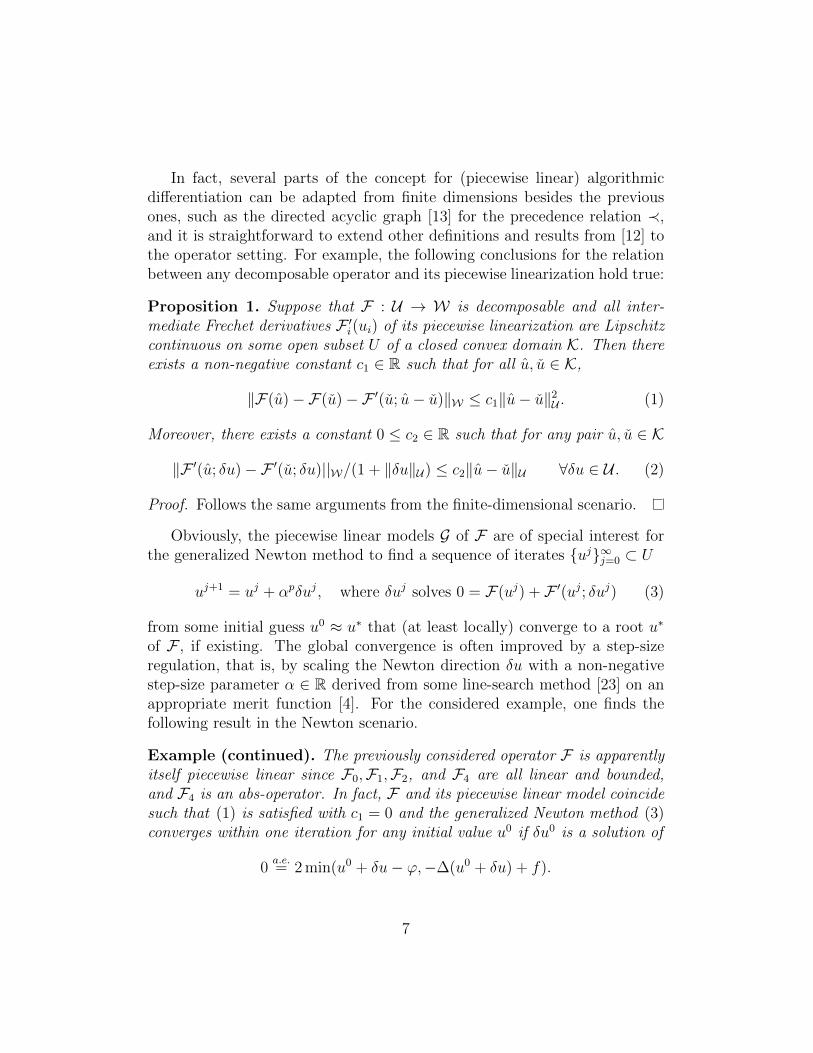
In fact, several parts of the concept for (piecewise linear) algorithmicdifferentiation can be adapted from finite dimensions besides the previousones, such as the directed acyclic graph [13] for the precedence relation ≺,and it is straightforward to extend other definitions and results from [12] tothe operator setting. For example, the following conclusions for the relationbetween any decomposable operator and its piecewise linearization hold true:

Proposition 1. Suppose that F : U → W is decomposable and all inter-mediate Frechet derivatives F ′i(ui) of its piecewise linearization are Lipschitzcontinuous on some open subset U of a closed convex domain K. Then thereexists a non-negative constant c1 ∈ R such that for all u, u ∈ K,

‖F(u)−F(u)−F ′(u; u− u)‖W ≤ c1‖u− u‖2U . (1)

Moreover, there exists a constant 0 ≤ c2 ∈ R such that for any pair u, u ∈ K

‖F ′(u; δu)−F ′(u; δu)||W/(1 + ‖δu‖U) ≤ c2‖u− u‖U ∀δu ∈ U . (2)

Proof. Follows the same arguments from the finite-dimensional scenario.

Obviously, the piecewise linear models G of F are of special interest forthe generalized Newton method to find a sequence of iterates uj∞j=0 ⊂ U

uj+1 = uj + αpδuj, where δuj solves 0 = F(uj) + F ′(uj; δuj) (3)

from some initial guess u0 ≈ u∗ that (at least locally) converge to a root u∗

of F , if existing. The global convergence is often improved by a step-sizeregulation, that is, by scaling the Newton direction δu with a non-negativestep-size parameter α ∈ R derived from some line-search method [23] on anappropriate merit function [4]. For the considered example, one finds thefollowing result in the Newton scenario.

Example (continued). The previously considered operator F is apparentlyitself piecewise linear since F0,F1,F2, and F4 are all linear and bounded,and F4 is an abs-operator. In fact, F and its piecewise linear model coincidesuch that (1) is satisfied with c1 = 0 and the generalized Newton method (3)converges within one iteration for any initial value u0 if δu0 is a solution of

0a.e.= 2 min(u0 + δu− ϕ,−∆(u0 + δu) + f).

7

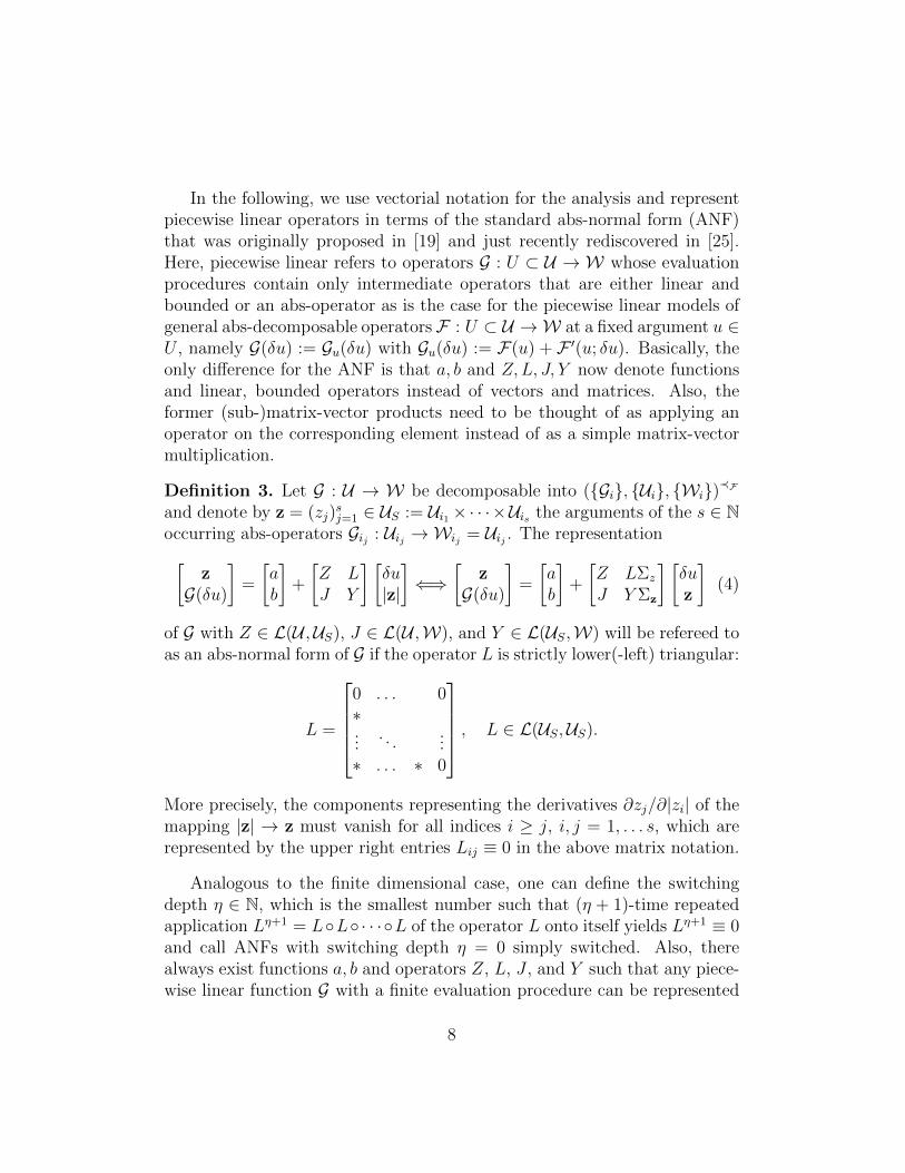
In the following, we use vectorial notation for the analysis and representpiecewise linear operators in terms of the standard abs-normal form (ANF)that was originally proposed in [19] and just recently rediscovered in [25].Here, piecewise linear refers to operators G : U ⊂ U → W whose evaluationprocedures contain only intermediate operators that are either linear andbounded or an abs-operator as is the case for the piecewise linear models ofgeneral abs-decomposable operators F : U ⊂ U → W at a fixed argument u ∈U , namely G(δu) := Gu(δu) with Gu(δu) := F(u) + F ′(u; δu). Basically, theonly difference for the ANF is that a, b and Z,L, J, Y now denote functionsand linear, bounded operators instead of vectors and matrices. Also, theformer (sub-)matrix-vector products need to be thought of as applying anoperator on the corresponding element instead of as a simple matrix-vectormultiplication.

Definition 3. Let G : U → W be decomposable into (Gi, Ui, Wi)≺F

and denote by z = (zj)sj=1 ∈ US := Ui1×· · ·×Uis the arguments of the s ∈ N

occurring abs-operators Gij : Uij →Wij = Uij . The representation[zG(δu)

]=

[ab

]+

[Z LJ Y

] [δu|z|

]⇐⇒

[zG(δu)

]=

[ab

]+

[Z LΣz

J Y Σz

] [δuz

](4)

of G with Z ∈ L(U ,US), J ∈ L(U ,W), and Y ∈ L(US,W) will be refereed toas an abs-normal form of G if the operator L is strictly lower(-left) triangular:

L =

0 . . . 0∗...

. . ....

∗ . . . ∗ 0

, L ∈ L(US,US).

More precisely, the components representing the derivatives ∂zj/∂|zi| of themapping |z| → z must vanish for all indices i ≥ j, i, j = 1, . . . s, which arerepresented by the upper right entries Lij ≡ 0 in the above matrix notation.

Analogous to the finite dimensional case, one can define the switchingdepth η ∈ N, which is the smallest number such that (η + 1)-time repeatedapplication Lη+1 = LL · · ·L of the operator L onto itself yields Lη+1 ≡ 0and call ANFs with switching depth η = 0 simply switched. Also, therealways exist functions a, b and operators Z, L, J , and Y such that any piece-wise linear function G with a finite evaluation procedure can be represented

8

as an ANF. If G is a piecewise linear model F(u) + F ′(u; δu) of an operatorF : U → W then the quantities of the ANF usually also depend on theargument u ∈ U :

a = a(u) = (a1(u), a2(u), . . . , as(u)) : U → U s, b = b(u) : U → W

and the operators Z = Z(u), L = L(u), J = J(u), Y = Y (u) satisfy

u ∈ U → Z(u) ∈ L(U ,US), u ∈ U → J(u) ∈ L(U ,W),

u ∈ U → L(u) ∈ L(US,US), u ∈ U → Y (u) ∈ L(US,W).

Although this dependence should always be kept in mind, it will not beexplicitly stated in the following, in order to avoid cumbersome notation.Assuming that W ≡ U and that the operator J is invertible with a corre-sponding inverse operator J−1, one can use the Schur-complement operator

S = L− ZJ−1Y ∈ L(U s,U s)

to define a modulus fixed-point equation on the arguments z ∈ U s of theabs-operators by

[I − SΣz]z = a− ZJ−1b, (5)

as was pointed out in [19, 25]. The latter equation is solved by a limitz∗ = limk→∞ zk of the modulus fixed-point iteration

zk+1 := [I − SΣzk ]−1(a− ZJ−1b) (6)

if this limit exists and was found for some initial guess z0 ∈ US (e.g. z0 = a).The solution z∗ then provides a solution

δu = −J−1[b+ Y |z∗|] (7)

of the ANF for the prescribed function value 0 = G(δu). However, theconvergence of the fixed-point iteration to a fixed point z∗ depends on theentries of the ANF at u and the initial value z0, as was observed in [25].

Example (continued). An ANF for the piecewise linear model of the pre-viously considered F at u and some directional increment δu is given by[

z2G(δu)

]=

[u− ϕ+ ∆u− fu− ϕ−∆u+ f

]+

[I + ∆ 0I −∆ −I

] [δu|z|

].

9

Obviously, only a := u − ϕ + ∆u − f and b := u − ϕ − ∆u + f depend onu, whereas Z := I + ∆, L := 0, J := I −∆, and Y := −I are independentof u. Since the operator J = (I + ∆) is invertible, one can use its inversemapping J−1 = (I + ∆) to define the modulus fixed-point equation (6) withS = 0− (I+ ∆) (I+ ∆)−1 (−I)Σz to find a direction δu with G(δu) = 0for the generalized Newton method (3).

Clearly, the advantage of this approach, namely, first formulating theANF in infinite dimensions instead of using a first-discretize-then-optimizeapproach, is that the structure of the considered problems can be exploited.In detail, the equations can now be treated in the correct spaces and solved byappropriate procedures, for example by some multigrid methods to improvethe efficiency of the resulting algorithms. At least for the previous example,one can also benefit from the fact that Z and J−1 are commutative operatorsand reformulate the fixed-point equation in a more numerical efficient way

[J − ZΣzk ]zk+1 = Ja− Zb, (8)

which can be iteratively solved and avoids dense matrix approximations ofthe inverse Laplace operator (or modifications) in the discrete formulationlater on. However, there is no reason that J should be invertible at all. Forthis case, Griewank suggested in [12] using the simple identity

δu = |δu+ |δu|| − |δu|, (9)

or modifications of it, to define an ANF, where the corresponding lower leftblock is invertible, which inspires the definition of an extended ANF:

Definition 4. Let G : U ⊂ U → U be a decomposable operator that isrepresented by the ANF (4) and Γ = Γ(u) ∈ L(U ,U) a given operator thatmight depend on u. Then the representation

zzzG(δu)

=

a00b

+

Z LΣz 0 0

J − Γ 0 0 0J − Γ 0 Σz 0

Γ Y Σz −Σz Σz

δxzzz

(10)

is called an extended abs-normal form (of its original ANF w.r.t. to Γ) ,where Σz and Σz, Σz are the abs-operators for the original switching functionsz ∈ US and the additional variables z, z in some appropriate space U , U ⊇ U ,respectively.

10

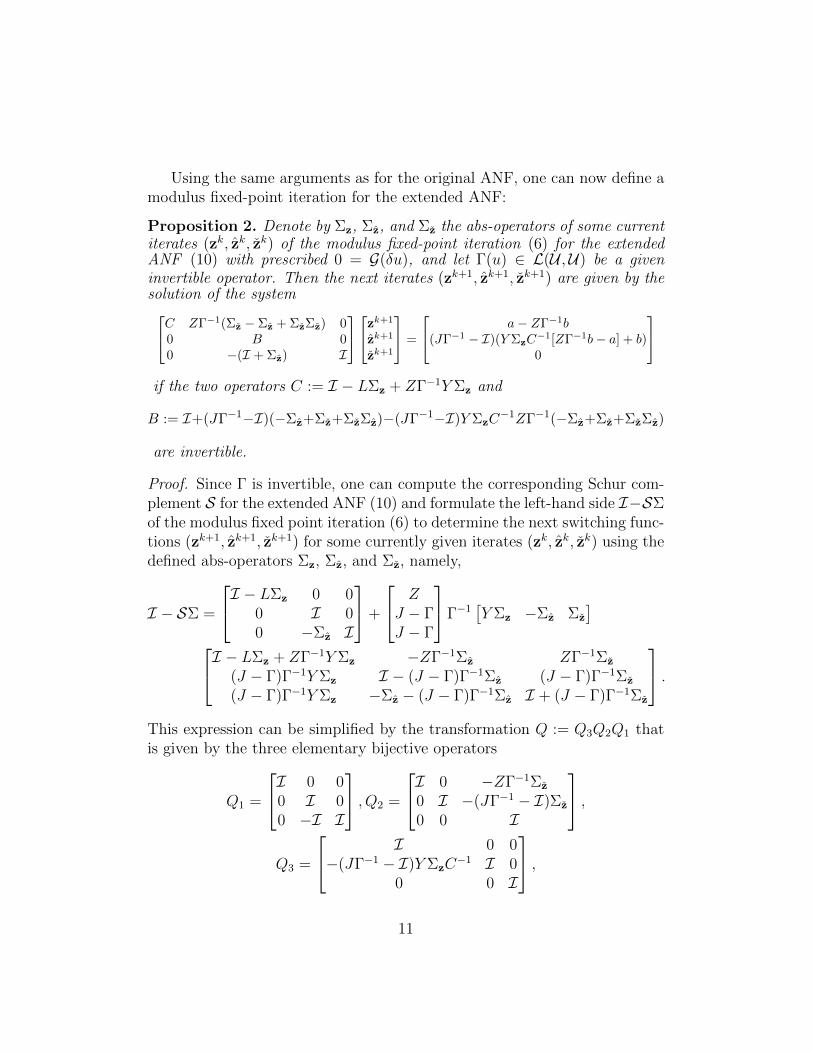
Using the same arguments as for the original ANF, one can now define amodulus fixed-point iteration for the extended ANF:

Proposition 2. Denote by Σz, Σz, and Σz the abs-operators of some currentiterates (zk, zk, zk) of the modulus fixed-point iteration (6) for the extendedANF (10) with prescribed 0 = G(δu), and let Γ(u) ∈ L(U ,U) be a giveninvertible operator. Then the next iterates (zk+1, zk+1, zk+1) are given by thesolution of the systemC ZΓ−1(Σz − Σz + ΣzΣz) 0

0 B 00 −(I + Σz) I

zk+1

zk+1

zk+1

=

a− ZΓ−1b(JΓ−1 − I)(Y ΣzC

−1[ZΓ−1b− a] + b)0

if the two operators C := I − LΣz + ZΓ−1Y Σz and

B := I+(JΓ−1−I)(−Σz+Σz+ΣzΣz)−(JΓ−1−I)Y ΣzC−1ZΓ−1(−Σz+Σz+ΣzΣz)

are invertible.

Proof. Since Γ is invertible, one can compute the corresponding Schur com-plement S for the extended ANF (10) and formulate the left-hand side I−SΣof the modulus fixed point iteration (6) to determine the next switching func-tions (zk+1, zk+1, zk+1) for some currently given iterates (zk, zk, zk) using thedefined abs-operators Σz, Σz, and Σz, namely,

I − SΣ =

I − LΣz 0 00 I 00 −Σz I

+

ZJ − ΓJ − Γ

Γ−1[Y Σz −Σz Σz

]I − LΣz + ZΓ−1Y Σz −ZΓ−1Σz ZΓ−1Σz

(J − Γ)Γ−1Y Σz I − (J − Γ)Γ−1Σz (J − Γ)Γ−1Σz

(J − Γ)Γ−1Y Σz −Σz − (J − Γ)Γ−1Σz I + (J − Γ)Γ−1Σz

.This expression can be simplified by the transformation Q := Q3Q2Q1 thatis given by the three elementary bijective operators

Q1 =

I 0 00 I 00 −I I

, Q2 =

I 0 −ZΓ−1Σz

0 I −(JΓ−1 − I)Σz

0 0 I

,Q3 =

I 0 0−(JΓ−1 − I)Y ΣzC

−1 I 00 0 I

,11

where the last one exists only if C = I − LΣz + ZΓ−1Y Σz is invertible.Thus, applying the transformation Q on both sides of the modulus fixedpoint iteration for the extended ANF does not alter the solution and yieldsthe desired result with the stated operator B.

Note that the assumption “C is invertible” in the proposition can alwaysbe achieved by choosing Γ in such a way that ‖Γ−1‖ is sufficiently small.However, the requirement of B being invertible cannot be always guaranteedsince, for example, in the case J = 0, Σz = 0 and −Σz + Σz + ΣzΣz = Ione finds B = 0. Furthermore, by considering the extended ANF in orderto resolve the issue of defining the modulus fixed-point iteration in case ofsingular J , one introduces a number of additional switching variables thatmight increase the likelihood of divergence of the modulus fixed point iter-ation in terms of cycling [25]. Moreover, the system might not be solvableat all, for example, under the previous assumptions with b 6= 0. Therefore,the algorithm in the next section is stated as general as possible to allow fordifferent fallback options (see [2, 3, 20]) in case of problems like the following.

Example 2. For some prescribed functions f , ϕl, and ϕu with ϕu ≥ ϕl,consider the modified linear complementarity problem

0 ≤ +u(x)− ϕl(x) ⊥ −∆u(x) + f(x) ≥ 0 and

0 ≤ −u(x) + ϕu(x) ⊥ +∆u(x)− f(x) ≥ 0 for almost all x ∈ Ω,

which requires −∆u + f = 0 to be satisfied whenever u is (strictly) betweenits lower or upper bound, ϕl and ϕu, respectively. It can be written as

0a.e.= F(u) = min [min[u− ϕl,−∆u+ f ],min[−u+ ϕu,∆u− f ]]

such that its piecewise linear model G(δu) = F(u) + F ′(u; δu) at u,

min [min [u+ δu− ϕl,−∆[u+ δu] + f ],min[−u− δu+ ϕu,∆[u+ δu]− f ]]] ,

is represented by an ANF with a singular smooth part J = 0. The quantitiesof the extended ANF (10) for the piecewise linear model of the modified linearcomplementarity problem are given by

a =

+u− ϕl + ∆u− f−u+ ϕu −∆u+ f

2(u−∆u+ f)− ϕl − ϕu

, Z =

+I + ∆−I −∆2(I −∆)

, L =

0 0 00 0 0−I I 0

b =

[ϕu − ϕl

], J =

[0], and Y =

[−I −I −I

].

12

3 Nonsmooth multigrid method

This section contains a multigrid method for the numerically efficient solutionof F(u) = 0 for some abs-factorizable operator F : U ⊂ U → U thatrepresents some nonsmooth PDE. The proposed method follows an approachsimilar to the original multigrid method [14, 17], and thus its structure mainlycoincides with the one in the smooth case. For simplicity, only piecewise-linear functions G : U ⊂ U → U are considered that arise as piecewise-linearmodels G(δu) = F(u) + F ′(u; δu) of a nonlinear operator F . In the smoothcase, the equality G(δu) = 0 is approximated by a discretized linear equationG(δu) = 0, which can be written as

Alδul = ql (11)

for some appropriate discretization matrix Al representing the Jacobian ofF at u and corresponding right-hand side ql. Here, the superscripts l ∈ Nindicate the current discretization level l so that l− 1 and l+ 1 represent thenext coarser and finer discretization level, respectively. Consequently,

Rl,l−1u : U l → U l−1 (Rl,l−1

z : U lS → U l−1S )

denotes the restriction operator, which maps elements from the space of fine-grid functions U l (U lS) to the corresponding elements in the space of coarsegrid functions U l−1 (U l−1

S ); and, analogously, the prolongation operator isdenoted by

P l−1,lu : U l−1 → U l (P l−1,l

z : U l−1S → U lS).

In particular, the prolongation and restriction usually satisfy the equalityRl,l−1u (P l−1,l

u (u)) = u(Rl,l−1

z (P l−1,lz (z)) = z

), namely, the application of a

restriction on a prolonged element from the coarse space is the element itself(in the coarse space). Using this notation, one can state the key ingredientsof the nonsmooth multigrid algorithm, that is, the full multigrid method, thebasic multigrid method, and the simple V-Cycle given by Algorithms 1, 2,and 3, respectively.

13

Algorithm 1 [zl, ul] = FullMG[lmax, l, lmin, zl, ul, ε,maxiter,maxmgv]

1: for l = l, . . . , lmin + 1 do2: Restrict zl−1 := Rl,l−1

z (zl) and ul−1 := Rl,l−1u (ul)

3: end for4: for l = lmin, . . . , lmax do5: [zl, ul, f lag] := MGV[l, lmin, z

l, ul, ε,maxiter,maxmgv]6: if l < lmax then7: Project zl := Dl(zl)

8: Prolong zl+1 := P l,l+1z (zl) and ul+1 := P l,l+1

u (ul)9: end if

10: end for

The key difference between the original full multigrid method for thesmooth case (see [14, 17]) and the presented method FullMG is that insteadof modifying u directly by solving the residual equations for (11) on thecoarser grids to find a suitable correction of δul, one applies the V-cycle onthe switching variables z depicted in Figure 1, which is then used to computea correction of δul at each level l.

Algorithm 2 [zl, ul, f lag] = MGV[l, lmin, zl, ul, ε,maxiter,maxmgv]

1: flag := false; iter = 1;2: while (flag == false)&&(iter ≤ maxmgv) do3: Set δul := 04: [zl, δul, f lag] := VCycle[l, lmin, z

l, ul, δul, ε,maxiter]5: Update ul := ul + δul; iter = iter + 1;6: end while

In detail, for some given initial approximations ul and zl on the grid l,the nonsmooth VCycle used in the multigrid cycle MGV differs from theoriginal method in that instead of evaluating the discretization matrix Al foreach level l, one evaluates in evalANF the abs-normal form (4) of G at ul foreach level l and performs the restriction, prolongation, and projection on thevariables z, u, δu (lines 5,7,8). The motivation for the projection operator

Dl : U lS → U lS

will be explained in the next section, as well as an appropriate choice for theprolongation and restriction operators P l−1,l and Rl,l−1, respectively.

14

Algorithm 3 [zl, δul, f lag] = VCycle[l, lmin, zl, ul, δul, ε,maxiter]

1: Evaluate [a, b, Z, L, J, Y ] := evalANF[l, ul, δul]2: if (l ≤ lmin) then maxiter = +∞;3: else4: [zl, δul, f lag] := solveANF[l, a, b, Z, L, J, Y, zl, δul, ε,maxiter]5: Project zl := Dl(zl)

6: Restrict zl−1 := Rl,l−1z (zl), ul−1 := Rl,l−1

u (ul), and δul−1 := Rl,l−1u (δul)

7: [zl−1, δul−1] := VCycle[l − 1, lmin, zl−1, ul−1, δul−1, ε,maxiter]

8: Project zl−1 := Dl(zl−1)

9: Prolong zl := P l−1,lz (zl−1) and δul := P l−1,l

u (δul−1)10: end if11: [zl, δul, f lag] := solveANF[l, a, b, Z, L, J, Y, zl, δul, ε,maxiter]

The method solveANF in the V-cycle given by Algorithm 4 correspondsto a smoothing operator on the current grid level that is usually appliedin smooth multigrid methods (e.g., a Jacobi, Gauss-Seidel, or Richardsonmethod). But instead of improving the linear residual equation of (11) as itis done in the smooth case, now one or more steps of the modulus fixed-pointiteration FPIter (Eq. (6)) are performed to find a better approximationzl. The latter approximation zl is then used to compute an update δul forthe multigrid algorithm 2 using Equation (7). In fact, the components ofthe multigrid algorithm are designed in such a way that any of the proposediterations from [2, 3, 6, 25, 20] (e.g., also the Block-Seidel iteration) can beencoded in the method FPiter to solve the ANF and allow for alternativesin the case of singular J .

Algorithm 4 [zl, δul, f lag] = solveANF[l, a, b, Z, L, J, Y, zl, δul, ε,maxiter]1: iter := 0, flag := false2: while (flag == false) and (iter < maxiter) do3: iter := iter + 14: [zlnew, δu

lnew] := FPIter[l, a, b, Z, L, J, Y, zl, δul]

5: if (‖zl − zlnew‖US < tol) then flag := true6: end if7: Update zl := zlnew and δul := δulnew8: end while

15

Nested VCycle with MGV for the linear solve within FPIterLevel l

VCycle-Step for the switching variables z

Project evalANF Restrict/ProlongatesolveANF

lmax

lmin

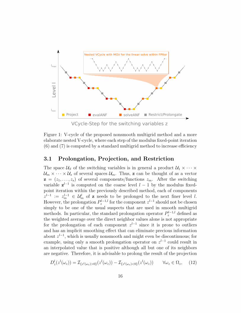
Figure 1: V-cycle of the proposed nonsmooth multigrid method and a moreelaborate nested V-cycle, where each step of the modulus fixed-point iteration(6) and (7) is computed by a standard multigrid method to increase efficiency

3.1 Prolongation, Projection, and Restriction

The space US of the switching variables is in general a product U1 × · · · ×Um × · · · × Us of several spaces Um. Thus, z can be thought of as a vectorz = (z1, . . . , zs) of several components/functions zm. After the switchingvariable zl−1 is computed on the coarse level l − 1 by the modulus fixed-point iteration within the previously described method, each of componentszl−1 := zl−1

m ∈ U lm of z needs to be prolonged to the next finer level l.However, the prolongation P l−1,l

z for the component zl−1 should not be chosensimply to be one of the usual suspects that are used in smooth multigridmethods. In particular, the standard prolongation operator P l−1,l

z defined asthe weighted average over the direct neighbor values alone is not appropriatefor the prolongation of each component zl−1 since it is prone to outliersand has an implicit smoothing effect that can eliminate precious informationabout zl−1, which is usually nonsmooth and might even be discontinuous; forexample, using only a smooth prolongation operator on zl−1 could result inan interpolated value that is positive although all but one of its neighborsare negative. Therefore, it is advisable to prolong the result of the projection

Dlz(z

l(ωz)) = Izl(ωz)>0(zl(ωz))− Izl(ωz)<0(z

l(ωz)) ∀ωz ∈ Ωz, (12)

16

which yields the point-wise sign of z, namely, Dlz(z(ωz)) ∈ −1, 0, 1 over the

appropriate domain Ωz 3 ωz. Alternatively, one can also use the ε-projectionfor sufficiently small ε ∈ R+

Dlz,ε(z

l(ωzl)) = Izl(ωz)>εzl(ωz)− Izl(ωz)<−εz

l(ωzl) ∀ωz ∈ Ωz

to compensate for numerical floating-point errors, which make it hard toexactly verify zl−1 = 0. These two projection variants are based on theobservation that only the sign of zl over the corresponding domain Ωz 3 ωzland not its actual value is needed to define the first step of modulus fixed-point iteration at the next finer level. However, the correctness and thequality of the result from the ε-projection Dl

z,ε strongly depend on the scalingof zl and the “right” choice of ε, which is usually unknown. Therefore, wesuggest using the exact sign projection Dl

z = Dlz,0, which often provides

sufficiently accurate results and avoids the task of finding a good estimatefor ε (as can be seen for the numerical examples later on). The prolongationfrom the coarse to the fine grid is achieved by some suitable prolongationoperator P l−1,l that leaves the value for every existing grid-point unchangedand assigns to every new point an average value of its neighbors. For example,in the 2D case for a square domain Ωz, which is discretized by an equidistantgrid with N (l−1) discretization points in one direction on the level l − 1, onecan use the nine-point prolongation [17] given by

zl2i,2j = zl−1i,j ∀ i = 0 . . . N (l−1), ∀ j = 0 . . . N (l−1),

zl2i+1,2j = 12

(zl−1i,j + zl−1

i+1,j

)∀ i = 0 . . . N (l−1) − 1, ∀ j = 0 . . . N (l−1),

zl2i,2j+1 = 12

(zl−1i,j + zl−1

i,j+1

)∀ i = 0 . . . N (l−1), ∀ j = 0 . . . N (l−1) − 1,

zl2i+1,2j+1 = 14

(zl−1i,j + zl−1

i,j+1 + zl−1i,j + zl−1

i+1,j + zl−1i+1,j+1

)∀ i, j = 0 . . . N (l−1) − 1.

(13)

This combination of projection and prolongation on zl−1 has the simple effectthat the interpolated values zli,j of the refined zl are given by the average signof its direct neighbors’ Ni,j values on the coarse grid, or more precisely

P l−1,lz (Dl−1(zl−1

i,j ))) =

−1, if

∑ω∈Nij

sign(zl−1(ω)) < 0

0, if∑

ω∈Nijsign(zl−1(ω)) = 0

+1, if∑

ω∈Nijsign(zl−1(ω)) > 0

.

On the one hand, this behavior is beneficial for problems with domains Ωz

that consist of larger subsets, where z has the same sign, such that elements

17

in the relative interior of these subsets are assigned the same signature as themajority of it’s neighbors and that elements with the same number of neigh-bors with positive and negative signature are set to the ‘neutral’ sign zero (cf.Figure 2). On the other hand, this effect might introduce wrong results, forexample in the case of structures that resolve only on finer resolutions or havecorners/isolated points. The latter artificially introduced errors then requireadditional correction steps in terms of the modulus fixed-point iteration onthe finer grid. Nevertheless, at least for the numerical examples consideredin Section 4, the first-project-then-prolong strategy dramatically reduces theoverall number of fixed-point iterations and increases the efficiency of theproposed multigrid method.

In an analogous way, one can define the coarse approximations zl−1 of zl

on the previously projected values Dl(zl) using either a (weighted version ofthe) nine-point restriction operator [17]

zl−1i,j =

1

4zl2i,2j +

1

16

(zl2i−1,2j−1 + zl2i−1,2j+1 + zl2i+1,2j−1 + zl2i+1,2j+1

)+

1

8

(zl2i,2j−1 + zl2i,2j+1 + zl2i−1,2j + zl2i+1,2j

),∀i, j = 1 . . . N (l−1) − 1,

(14)

or, alternatively, the trivial restriction zl−1 = Rl,l−1z (zl) that is given by

zl−1i,j = zl2i,2j, for all i, j = 0 . . . N (l−1), (15)

where every second element in the relative interior is simply dismissed.

1

1.5

2

2.5

3

1

1.5

2

2.5

3

−2

0

2

4

6

8

10

ω1

z

z

ω2

z

zl−

1

1

2

3

4

5

1

2

3

4

5

−1

−0.8

−0.6

−0.4

−0.2

0

0.2

0.4

0.6

0.8

1

ω1

z

z

ω2

z

zl−

1

1

2

3

4

5

1

2

3

4

5

−1

−0.8

−0.6

−0.4

−0.2

0

0.2

0.4

0.6

0.8

1

ω1

z

z

ω2

z

zl−

1

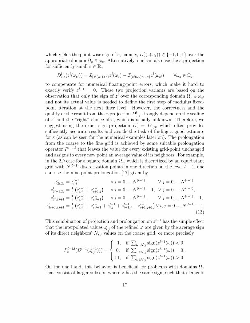
Figure 2: Visualization of a function zl−1 (left), its projected-prolonged-projection Dl

z(Pl−1,lz (Dl−1

z (zl−1))) (middle), and its simply projected-prolongation Dl

z(Pl−1,lz (zl−1)) (right). Here, the last projection Dl

z is dueto the projection that is implicitly given by the definition of Σ.

18

3.2 Modified V-Cycle/Successive-Refinement Method

As was observed in the previous subsection, the restriction/prolongation incombination with the projection causes artificial errors that might lead toadditional correction steps by the modulus fixed-point iteration on the nextconsidered level l. Specifically, several redundant steps could be avoided andare needed only to undo the effects of the inappropriate smoothing effectintroduced by (13) and (14). Therefore, instead of the full multigrid method,we propose to simply use the modified MGV method without the solveANFin line 4, where the number of maximum iterations is set to infinity and themaximum of MGV cycles equals one (i.e., maxiter = ∞ and maxmgv =1). In other words, one performs a V-cycle, where the modulus fixed-pointiteration is fully converged to its limit zl∗ on each level l before it is prolongedand projected on the next finer level l+1 after eventually restricting the initialapproximation to the coarsest level lmin, such that δu∗ = δu(z∗) then solvesG(u+ δu∗) = 0 on the finest grid lmax.

Obviously, the most expensive part of this algorithm is the solution ofthe ANF in solveANF, which requires the solution of the linear equation

Alzlnew := [I − SΣzlold]zlnew = (a− ZJ−1b) := ql

for every modulus fixed-point iteration step FPIter on each level l, in orderto determine the next switching variables zlnew based on the previous estimatezlold or the computation of δul according to (7). The latter linear equationscan be solved again in a multigrid fashion, which then leads to the nestedapproach that was also depicted in Figure 1. However, the same objectionsconcerning the undesired smoothing effect of the MG-cycle for the linear solvepartly hold true. Another improvement that can be applied for all methods,which might pay off in the case of an expensive function evaluation, is thatthe ANF is evaluated only once on the finest level and then gets restricted tothe coarser grids. Also, the ANF does not need to be reevaluated from scratchafter updating u = u+ δu∗ after one modified MGV cycle; instead one canset a := a+ Zδu∗ and b := b+ Jδu∗ to find the new residual approximation0 = Gu(δu∗ + δu) for the next cycle3 in the piecewise linear case.

3Note that in general Gu(δu∗ +δu) 6= Gu+δu∗(δu) if Gx denotes the piecewise lineariza-tion of a nonlinear, nonsmooth function F at x such that the proposed update of a and bis, in fact, needed to find the exact residual equation of the ANF at u.

19

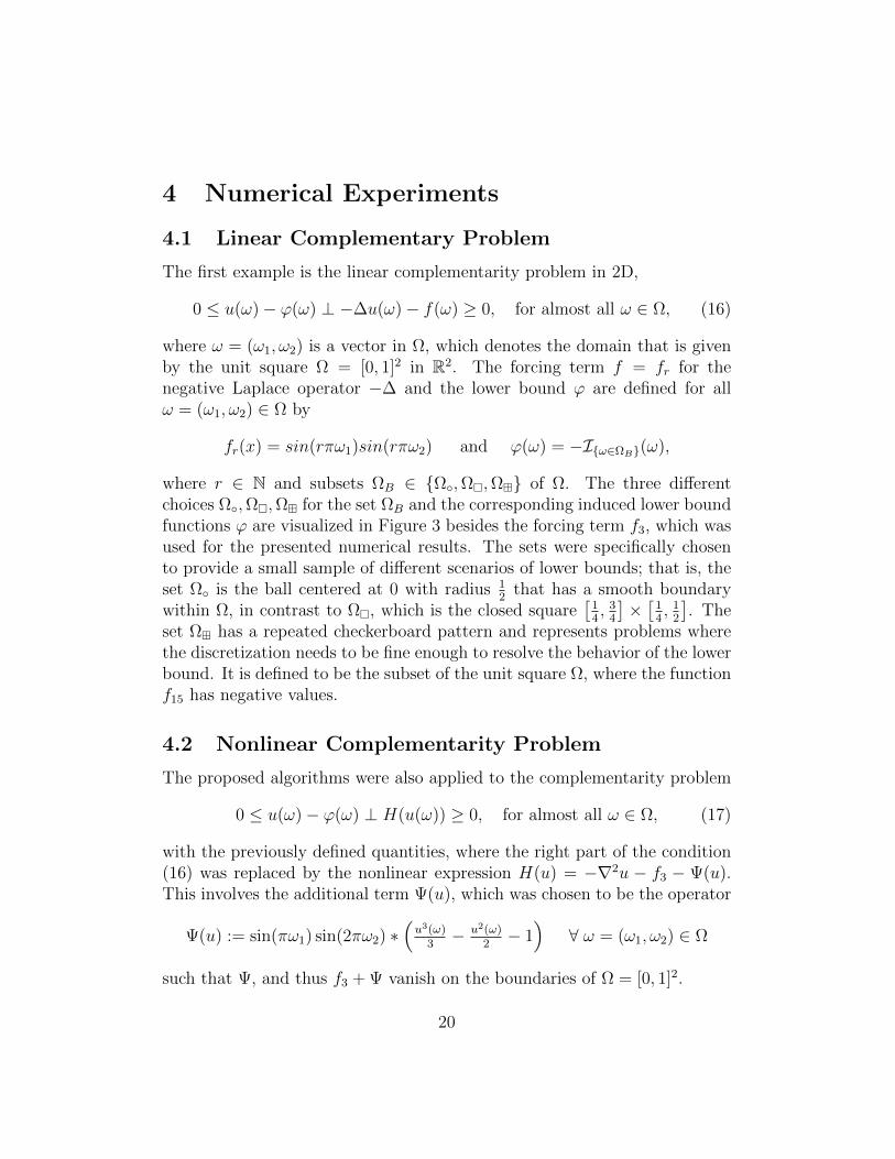
4 Numerical Experiments

4.1 Linear Complementary Problem

The first example is the linear complementarity problem in 2D,

0 ≤ u(ω)− ϕ(ω) ⊥ −∆u(ω)− f(ω) ≥ 0, for almost all ω ∈ Ω, (16)

where ω = (ω1, ω2) is a vector in Ω, which denotes the domain that is givenby the unit square Ω = [0, 1]2 in R2. The forcing term f = fr for thenegative Laplace operator −∆ and the lower bound ϕ are defined for allω = (ω1, ω2) ∈ Ω by

fr(x) = sin(rπω1)sin(rπω2) and ϕ(ω) = −Iω∈ΩB(ω),

where r ∈ N and subsets ΩB ∈ Ω,Ω,Ω of Ω. The three differentchoices Ω,Ω,Ω for the set ΩB and the corresponding induced lower boundfunctions ϕ are visualized in Figure 3 besides the forcing term f3, which wasused for the presented numerical results. The sets were specifically chosento provide a small sample of different scenarios of lower bounds; that is, theset Ω is the ball centered at 0 with radius 1

2that has a smooth boundary

within Ω, in contrast to Ω, which is the closed square[

14, 3

4

]×[

14, 1

2

]. The

set Ω has a repeated checkerboard pattern and represents problems wherethe discretization needs to be fine enough to resolve the behavior of the lowerbound. It is defined to be the subset of the unit square Ω, where the functionf15 has negative values.

4.2 Nonlinear Complementarity Problem

The proposed algorithms were also applied to the complementarity problem

0 ≤ u(ω)− ϕ(ω) ⊥ H(u(ω)) ≥ 0, for almost all ω ∈ Ω, (17)

with the previously defined quantities, where the right part of the condition(16) was replaced by the nonlinear expression H(u) = −∇2u − f3 − Ψ(u).This involves the additional term Ψ(u), which was chosen to be the operator

Ψ(u) := sin(πω1) sin(2πω2) ∗(u3(ω)

3− u2(ω)

2− 1)

∀ ω = (ω1, ω2) ∈ Ω

such that Ψ, and thus f3 + Ψ vanish on the boundaries of Ω = [0, 1]2.

20

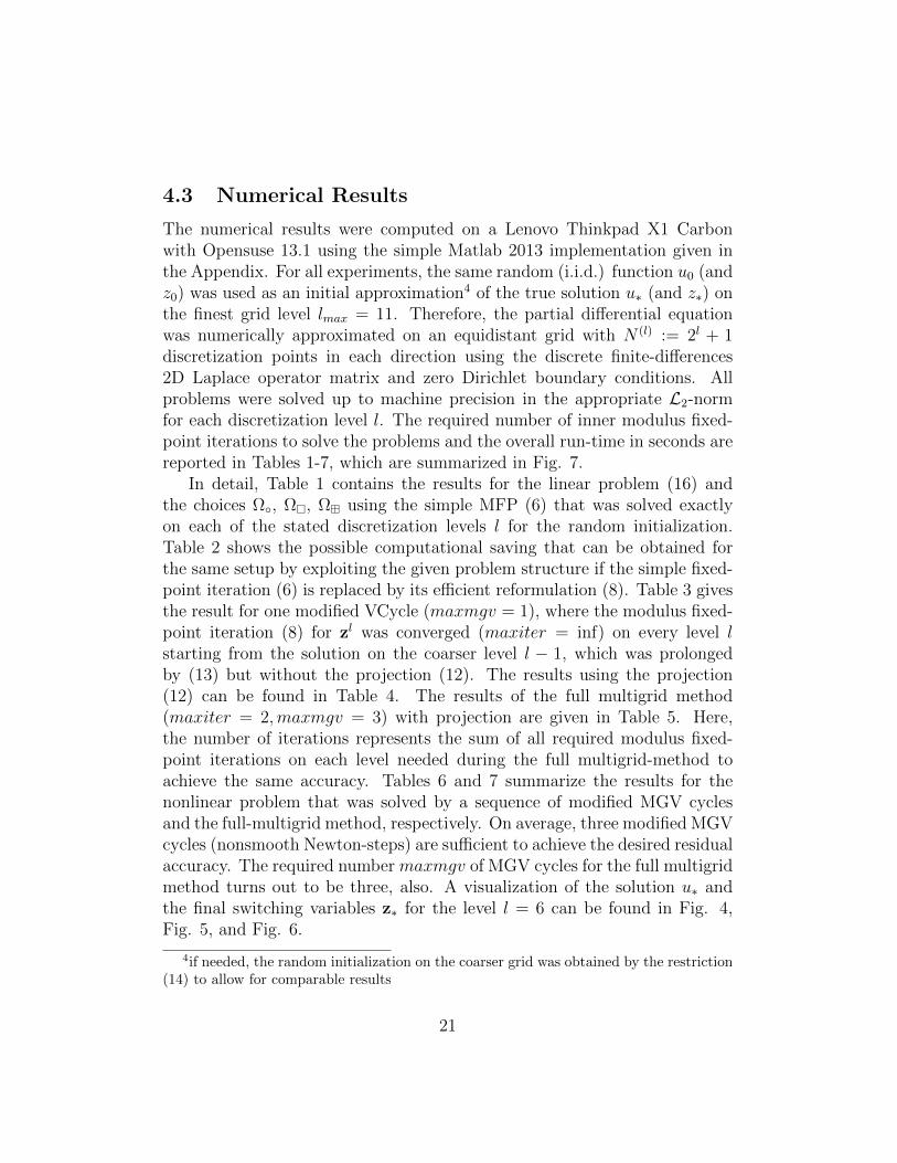
4.3 Numerical Results

The numerical results were computed on a Lenovo Thinkpad X1 Carbonwith Opensuse 13.1 using the simple Matlab 2013 implementation given inthe Appendix. For all experiments, the same random (i.i.d.) function u0 (andz0) was used as an initial approximation4 of the true solution u∗ (and z∗) onthe finest grid level lmax = 11. Therefore, the partial differential equationwas numerically approximated on an equidistant grid with N (l) := 2l + 1discretization points in each direction using the discrete finite-differences2D Laplace operator matrix and zero Dirichlet boundary conditions. Allproblems were solved up to machine precision in the appropriate L2-normfor each discretization level l. The required number of inner modulus fixed-point iterations to solve the problems and the overall run-time in seconds arereported in Tables 1-7, which are summarized in Fig. 7.

In detail, Table 1 contains the results for the linear problem (16) andthe choices Ω, Ω, Ω using the simple MFP (6) that was solved exactlyon each of the stated discretization levels l for the random initialization.Table 2 shows the possible computational saving that can be obtained forthe same setup by exploiting the given problem structure if the simple fixed-point iteration (6) is replaced by its efficient reformulation (8). Table 3 givesthe result for one modified VCycle (maxmgv = 1), where the modulus fixed-point iteration (8) for zl was converged (maxiter = inf) on every level lstarting from the solution on the coarser level l − 1, which was prolongedby (13) but without the projection (12). The results using the projection(12) can be found in Table 4. The results of the full multigrid method(maxiter = 2,maxmgv = 3) with projection are given in Table 5. Here,the number of iterations represents the sum of all required modulus fixed-point iterations on each level needed during the full multigrid-method toachieve the same accuracy. Tables 6 and 7 summarize the results for thenonlinear problem that was solved by a sequence of modified MGV cyclesand the full-multigrid method, respectively. On average, three modified MGVcycles (nonsmooth Newton-steps) are sufficient to achieve the desired residualaccuracy. The required number maxmgv of MGV cycles for the full multigridmethod turns out to be three, also. A visualization of the solution u∗ andthe final switching variables z∗ for the level l = 6 can be found in Fig. 4,Fig. 5, and Fig. 6.

4if needed, the random initialization on the coarser grid was obtained by the restriction(14) to allow for comparable results

21

The nested multigrid method was not considered in the numerical exper-iments in order to avoid any interference, but it is likely to provide furtherspeedup. Instead, all the occurring linear equations within the solveANFmethod were solved by Matlab’s backslash operator.

010

2030

4050

6070

0

20

40

60

80

−1

−0.8

−0.6

−0.4

−0.2

0

0.2

0.4

0.6

0.8

1

ω1z

f

ω2z

zl−

1

010

2030

4050

6070

0

20

40

60

80

−1

−0.9

−0.8

−0.7

−0.6

−0.5

−0.4

−0.3

−0.2

−0.1

0

ω1

z

Ωc

ω2

z

zl−

1

010

2030

4050

6070

0

20

40

60

80

−1

−0.9

−0.8

−0.7

−0.6

−0.5

−0.4

−0.3

−0.2

−0.1

0

ω1

z

Ωs

ω2

z

zl−

1

010

2030

4050

6070

0

20

40

60

80

−1

−0.9

−0.8

−0.7

−0.6

−0.5

−0.4

−0.3

−0.2

−0.1

0

ω1

z

Ωc

ω2

z

zl−

1

Figure 3: Right-hand-side f3, and the indicator functions induced by Ω, Ω,and Ω (from left to right).

Figure 4: Solution u of the linear complementarity problem for the lowerbounds induced by Ω, Ω, and Ω (from left to right).

22

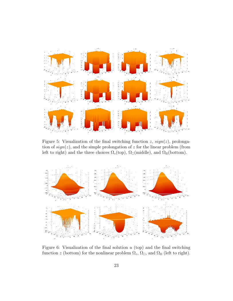
Figure 5: Visualization of the final switching function z, sign(z), prolonga-tion of sign(z), and the simple prolongation of z for the linear problem (fromleft to right) and the three choices Ω(top), Ω(middle), and Ω(bottom).

Figure 6: Visualization of the final solution u (top) and the final switchingfunction z (bottom) for the nonlinear problem Ω, Ω, and Ω (left to right).

23

1 2 3 4 5 6 7 8 9 10 110

5

10

15

20

25

30

35

40

45

50

FP

−It

era

tio

n

Discretization Level l

1 2 3 4 5 6 7 8 9 10 1110

−4

10−3

10−2

10−1

100

101

102

103

Tim

e (

seconds)

Discretization Level l

Figure 7: Visualization of the number of required FPIter (left) and overallrun-time in seconds (right) for each discretization level l reported in Table 1(yellow), Table 2 (light orange), Table 3 (dark orange), and Table 4 (red) forthe three different lowerbounds Ω (), Ω (), and Ω (×).

l ] Iter Time Ω ] Iter Time Ω ] Iter Time Ω

1 2 6.960000e-04 2 6.350000e-04 3 8.670000e-042 2 1.733000e-03 3 1.873000e-03 3 2.383000e-033 3 7.161000e-03 5 8.501000e-03 5 1.032100e-024 3 5.299700e-02 6 1.286270e-01 5 8.884200e-025 5 1.509989e+00 9 2.392125e+00 7 1.860127e+00

Table 1: Results for the linear problem (16) using the simple MFP (6),without projection, for the choices Ω, Ω, Ω solved on each level l.

l ] Iter Time Ω ] Iter Time Ω ] Iter Time Ω

1 2 6.020000e-04 2 6.100000e-04 3 7.960000e-042 2 1.085000e-03 3 1.532000e-03 3 1.571000e-033 3 4.504000e-03 5 7.382000e-03 5 7.394000e-034 3 5.249300e-02 5 9.025300e-02 6 1.022870e-015 2 5.411540e-01 5 1.353975e+00 8 2.140963e+00

Table 2: Results for the linear problem (16) using the efficient MFP (8),without projection, standard prolongation (13), and simple restriction (15),for the choices Ω, Ω, Ω solved on each level l.

24

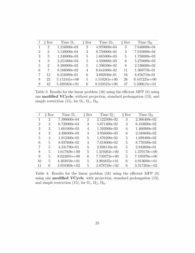
l ] Iter Time Ω ] Iter Time Ω ] Iter Time Ω

1 2 1.216000e-03 2 4.970000e-04 3 7.640000e-042 2 5.120000e-04 3 6.750000e-04 3 7.010000e-043 3 1.240000e-03 5 1.685000e-03 5 1.738000e-034 3 3.251000e-03 5 4.509000e-03 6 5.278000e-035 2 8.380000e-03 5 1.596500e-02 8 2.536600e-026 7 8.506000e-02 4 6.641000e-02 11 1.369770e-017 12 6.216080e-01 6 3.692940e-01 16 8.856710e-018 22 5.112441e+00 5 1.510281e+00 26 6.447225e+009 42 5.328563e+01 6 8.533525e+00 47 5.336615e+01

Table 3: Results for the linear problem (16) using the efficient MFP (8) usingone modified VCycle, without projection, standard prolongation (13), andsimple restriction (15), for Ω, Ω, Ω.

l ] Iter Time Ω ] Iter Time Ω ] Iter Time Ω

1 2 7.390000e-04 2 2.122500e-02 3 2.366400e-022 2 6.720000e-04 3 5.671400e-02 3 6.433000e-023 3 1.681000e-03 4 1.592000e-03 4 1.466000e-034 3 4.496000e-03 4 3.956000e-03 6 2.588600e-025 4 1.912300e-02 5 1.876200e-02 5 1.699400e-026 5 8.937600e-02 4 7.618000e-02 5 8.776500e-027 5 4.231790e-01 5 2.698110e-01 5 2.943600e-018 5 1.617928e+00 5 1.319262e+00 5 1.379170e+009 5 8.022691e+00 6 7.749272e+00 5 7.195976e+0010 5 4.403858e+01 5 3.904835e+01 6 4.913688e+0111 6 3.958369e+02 5 2.878728e+02 6 3.317204e+02

Table 4: Results for the linear problem (16) using the efficient MFP (8)using one modified VCycle, with projection, standard prolongation (13),and simple restriction (15), for Ω, Ω, Ω.

25

l ] Iter Time Ω ] Iter Time Ω ] Iter Time Ω

1 31 1.324390e-01 33 2.058090e-01 40 7.987100e-022 55 1.672640e-01 59 1.668160e-01 71 1.495700e-013 47 1.224120e-01 52 1.150760e-01 64 1.383930e-014 39 2.049110e-01 44 3.029320e-01 56 2.337380e-015 32 8.836760e-01 36 4.422830e-01 48 5.185170e-016 24 7.157060e-01 28 1.186067e+00 40 1.576971e+007 20 3.216956e+00 20 3.502826e+00 32 5.414041e+008 16 1.055167e+01 16 8.553483e+00 24 1.576412e+019 12 3.098891e+01 12 2.963045e+01 16 4.225638e+0110 8 1.139729e+02 8 1.176420e+02 8 1.208749e+0211 4 4.012236e+02 4 4.682104e+02 4 3.886089e+02

Table 5: Results for the linear problem (16) using the efficient MFP (8) usingthe Full multigrid, with projection, standard prolongation (13), and simplerestriction (15), for the choices Ω, Ω, Ω.

l ] Iter Time Ω ] Iter Time Ω ] Iter Time Ω

1 (2,2,2) 3.648100e-02 (2,2,2) 7.651100e-02 (3,3,3) 3.660200e-022 (2,2,2) 1.039410e-01 (2,2,2) 1.501190e-01 (4,4,4) 1.378060e-013 (3,3,3) 4.527000e-03 (4,4,4) 6.986000e-03 (3,3,3) 3.965000e-034 (4,4,4) 5.646800e-02 (4,4,4) 1.094530e-01 (7,7,7) 8.923100e-025 (4,4,4) 5.401000e-02 (5,5,5) 4.828000e-02 (5,5,6) 6.527600e-026 (5,4,4) 3.606830e-01 (5,5,5) 1.839210e-01 (5,5,5) 8.170460e-017 (6,6,6) 1.082465e+00 (5,5,5) 8.430270e-01 (5,5,5) 9.230070e-018 (4,4,4) 4.097798e+00 (5,5,5) 4.181277e+00 (5,5,5) 4.203123e+009 (5,5,5) 2.617473e+01 (5,6,6) 2.201599e+01 (6,6,6) 2.343003e+0110 (7,5,5) 1.584398e+02 (6,6,6) 1.361256e+02 (6,6,6) 1.321681e+0211 (8,9,9) 1.588478e+03 (6,6,6) 9.912651e+02 (6,6,6) 9.558356e+02

Table 6: Results for the nonlinear problem (17) using the efficient MFP (8)using modified V-cycle, with projection (12), standard prolongation (13),and simple restriction(15), for Ω, Ω, Ω, where the number of fixed-pointiterations is given for each of the three MGV cycles separately for all levelsl.

26

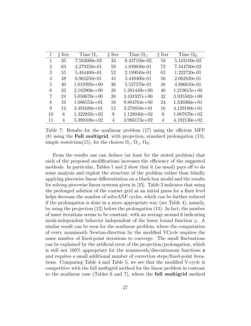
l ] Iter Time Ω ] Iter Time Ω ] Iter Time Ω

1 35 7.583000e-02 33 8.437100e-02 58 5.103100e-022 63 4.279350e-01 59 1.839830e-01 72 7.344700e-023 55 5.484400e-01 52 2.199040e-01 63 1.222720e-014 48 6.964250e-01 44 3.449400e-01 56 2.062820e-015 40 1.019395e+00 36 5.527570e-01 48 4.886610e-016 32 2.182906e+00 28 1.381449e+00 40 1.219615e+007 24 5.050670e+00 20 3.431927e+00 32 3.935502e+008 16 1.086553e+01 16 9.884764e+00 24 1.330366e+019 12 3.491688e+01 12 3.278858e+01 16 4.129180e+0110 8 1.322932e+02 8 1.128040e+02 8 1.087870e+0211 4 5.399108e+02 4 3.986173e+02 4 4.192130e+02

Table 7: Results for the nonlinear problem (17) using the efficient MFP(8) using the Full multigrid, with projection, standard prolongation (13),simple restriction(15), for the choices Ω, Ω, Ω.

From the results one can deduce (at least for the stated problem) thateach of the proposed modifications increases the efficiency of the suggestedmethods. In particular, Tables 1 and 2 show that it (as usual) pays off to dosome analysis and exploit the structure of the problem rather than blindlyapplying piecewise linear differentiation on a black-box model and the resultsfor solving piecewise linear systems given in [25]. Table 3 indicates that usingthe prolonged solution of the coarser grid as an initial guess for a finer levelhelps decrease the number of solveANF cycles, which can be further reducedif the prolongation is done in a more appropriate way (see Table 4), namely,by using the projection (12) before the prolongation (13). In fact, the numberof inner iterations seems to be constant, with an average around 6 indicatingmesh-independent behavior independent of the lower bound function ϕ. Asimilar result can be seen for the nonlinear problem, where the computationof every nonsmooth Newton-direction by the modified VCycle requires thesame number of fixed-point iterations to converge. The small fluctuationscan be explained by the artificial error of the projection/prolongation, whichis still not 100% appropriate for the nonsmooth/discontinuous functions zand requires a small additional number of correction steps/fixed-point itera-tions. Comparing Table 4 and Table 5, we see that the modified V-cycle iscompetitive with the full multigrid method for the linear problem in contrastto the nonlinear case (Tables 6 and 7), where the full multigrid method

27

seems to perform better, mainly because of the smaller number of fixed pointiterations on the finer grid.

5 Conclusion

In this paper, a multigrid method for nonsmooth problems was considered.It is based on ideas of the original multigrid method and techniques frompiecewise linear differentiation in finite dimensions. We assumed that theconsidered problems were abs-decomposable and their piecewise linearizationcan be written in abs-normal form. The abs-normal form allows for variousiterative schemes that can be applied to solve the resulting piecewise linearequation using some additional switching variables for each discretizationlevel. The overall method is based on a successive refinement strategy, where(approximate) solutions of the additional switching variables on a coarserlevels are used as initial approximations on a finer level. Since the switch-ing variables themselves are usually nonsmooth or even discontinuous, theirprolongation from the coarser to the finer level needs special treatment, asit was exemplified for a simple complementarity problem. It appears that a“correct” prolongation, restriction, and projection of these variables provide(almost) mesh-independent results allowing for an efficient solution of theproblem with up to 4,2 million degrees of freedom on the finest discretizationlevel in a reasonable time, which is comparable to the results5 of the differentapproaches presented in [26, 9, 11, 15]. The resulting method and strategiescould be used to solve time-dependent differential equations together withthe generalized mid-point rule [5], for example if the time integration involvessome nonsmooth UPWIND/QUICK scheme[27], which can be stated in termsof min and max. However, it is not clear whether the small average number ofmodulus fixed-point iterations observed for the considered example does holdtrue in general. If not, this would suggest further investigation of a more ap-propriate projection and prolongation strategy for nonsmooth/discontinuousfunctions. Also, different fallback options for singular J instead of using onlythe extended ANF should be investigated. Furthermore, different strategiesfor the nonlinear case should be part of future research directions, for exam-ple, comparing the presented Newton-MG with an MG-Newton scheme andan additional line-search for the globalization.

5if not better

28

Acknowledgment

This material is based upon work supported by the U.S. Department ofEnergy, Office of Science, under contract number DE-AC02-06CH11357. Theauthor is grateful to Zichao (Wendy) Di for several comments that helpedimprove the notation and Gail Pieper for her patient and precious corrections.

Appendix - Matlab Codes

This section contains parts of a simple MATLAB implementation for theproposed methods that were used to compute the presented results. Themethods coincide with the algorithms except for the difference in solveANFand FPIter, where the computation of δunew was detached from FPIter andis computed only once at the end of the fixed-point iteration, in order to avoidobsolete linear-solves and increase the overall efficiency.

Listing 1: V-Cycle methodf unc t i on [ z , Du ] = VCycle ( l , lmin , z , u , Du, to l , maxiter )

[ a , b , Z , L , J , Y] = evalANF( l , u , Du) ;i f l<=lmin

maxiter=1e3 ;e l s e

[ z , Du] = solveANF ( l , a , b , Z , L , J , Y, z , Du, to l , maxiter ) ;z=p ro j e c t z ( z , l ) ;z=r e s t r i c t z ( z , l ) ;u=r e s t r i c t u (u , l ) ;[ z , Du] = VCycle ( l - 1 , lmin , z , u , Du, to l , maxiter ) ;z=p ro j e c t z ( z , l - 1 ) ;z=pro longz ( z , l - 1 ) ;Du=prolongu (Du, l - 1 ) ;

end[ z , Du] = solveANF ( l , a , b , Z , L , J , Y, z , Du, to l , maxiter ) ;

r e turn

Listing 2: Multigrid cyclef unc t i on [ z , u ] = MGV( l , lmin , z , u , to l , maxiter , maxmgv)

f l a g =1; i =1;Du = 0 . ∗u ( : ) ;whi le ( f l a g ~=0)&&(i<=maxmgv)

[ z , Du] = VCycle ( l , lmin , z , u , Du, to l , maxiter ) ;u ( : ) = u ( : ) + Du ( : ) ;i=i +1;i f ( s ca lp rod ( l , Du( : ) , Du ( : ) ) <= to l )

f l a g =0;end

endreturn

29

Listing 3: Full multigrid methodf unc t i on [ z , u ] = FullMG( lmax , l cur , lmin , z , u , to l , maxiter , maxmgv)

f o r l=l cu r : - 1 : lmin+1z=pro j e c t z ( z , l ) ;z=r e s t r i c t z ( z , l ) ;u=r e s t r i c t u (u , l ) ;

endf o r l=lmin : 1 : lmax

[ z , u ]= MGV( l , lmin , z , u , to l , maxiter , maxmgv ) ;i f l<lmax

z=pro j e c t z ( z , l ) ;z=pro longz ( z , l ) ;u=prolongu (u , l ) ;

endend

return

Listing 4: Modified V-Cyclef unc t i on [ z , Du ]= modVCycle ( l , lmin , z , u , Du, t o l )

[ a , b , Z , L , J , Y]=evalANF( l , u , Du) ;i f l>lmin

z=pro j e c t z ( z , l ) ;z=r e s t r i c t z ( z , l ) ;u=r e s t r i c t u (u , l ) ;[ z , Du]= modVCycle ( l - 1 , lmin , z , u , Du, t o l ) ;z=p ro j e c t z ( z , l - 1 ) ;z=pro longz ( z , l - 1 ) ;Du=prolongu (Du, l - 1 ) ;

end[ z , Du] = solveANF ( l , a , b , Z , L , J , Y, z , Du, to l , i n f ) ;

r e turn

Listing 5: Modified Multigrid cyclef unc t i on [ z , u ] = modMGV( l , lmin , z , u , t o l )

Du=0 . ∗u ( : ) ;[ z , Du ] = modVCycle ( l , lmin , z , u , Du, t o l ) ;u ( : ) = u ( : ) + Du ( : ) ;

r e turn

Listing 6: solveANF methodf unc t i on [ z , Du]= solveANF ( l , a , b , Z , L , J , Y, z , Du, to l , maxiter )

i t e r =0; f l a g =1; t i c ;whi le ( ( f l a g ~=0)&&( i t e r<maxiter ) )

i t e r=i t e r +1;[ znew ] = FPIter ( a , b , Z , L , J , Y, z ( : ) , Du ( : ) ) ;t = z ( : ) - znew ( : ) ; r e s=sca lprod ( l , t ( : ) , t ( : ) ) ;i f res<t o l

f l a g = 0 ;end

z=znew ;endDu=-J\(b+Y∗abs ( znew ( : ) ) ) ; %For e f f i c i e n c y reason

return

30

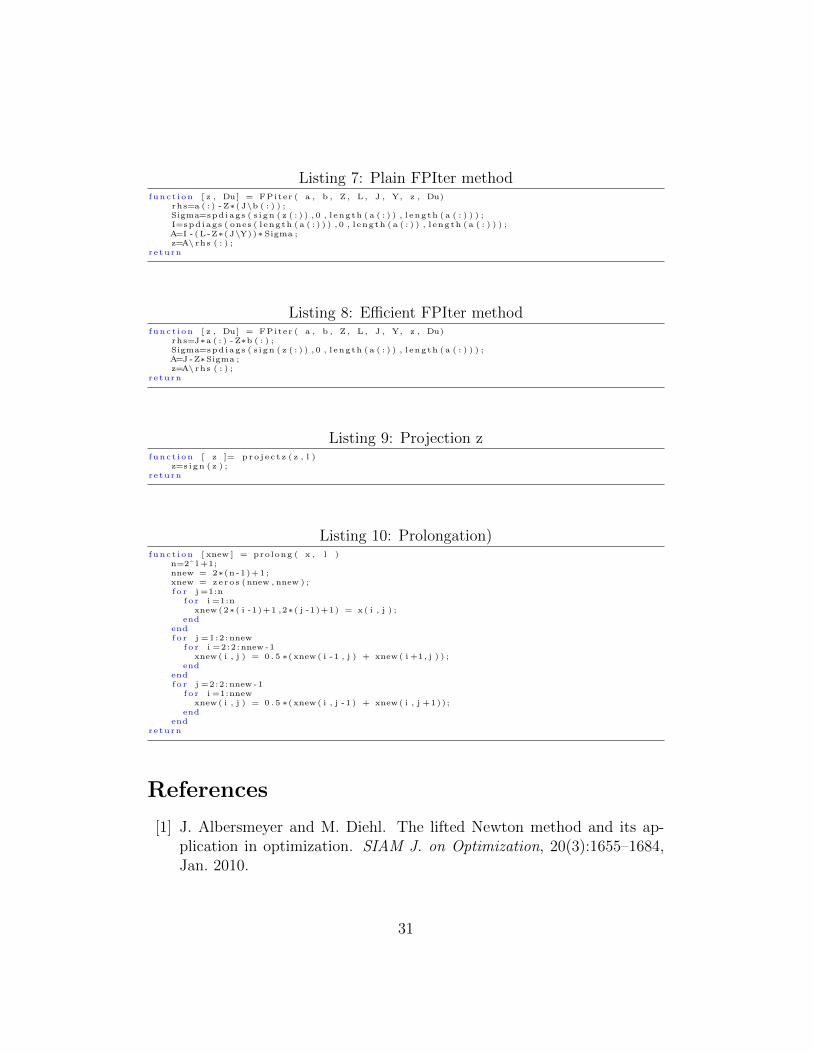
Listing 7: Plain FPIter methodf unc t i on [ z , Du] = FPiter ( a , b , Z , L , J , Y, z , Du)

rhs=a ( : ) - Z∗( J\b ( : ) ) ;Sigma=spd iags ( s i gn ( z ( : ) ) , 0 , l ength ( a ( : ) ) , l ength ( a ( : ) ) ) ;I=spd iags ( ones ( l ength ( a ( : ) ) ) , 0 , l ength ( a ( : ) ) , l ength ( a ( : ) ) ) ;A=I - (L-Z∗( J\Y))∗ Sigma ;z=A\ rhs ( : ) ;

r e turn

Listing 8: Efficient FPIter methodf unc t i on [ z , Du] = FPiter ( a , b , Z , L , J , Y, z , Du)

rhs=J∗a ( : ) - Z∗b ( : ) ;Sigma=spd iags ( s i gn ( z ( : ) ) , 0 , l ength ( a ( : ) ) , l ength ( a ( : ) ) ) ;A=J -Z∗Sigma ;z=A\ rhs ( : ) ;

r e turn

Listing 9: Projection zf unc t i on [ z ]= p ro j e c t z ( z , l )

z=s ign ( z ) ;r e turn

Listing 10: Prolongation)f unc t i on [ xnew ] = prolong ( x , l )

n=2ˆ l +1;nnew = 2∗(n -1)+1;xnew = ze ro s (nnew , nnew ) ;f o r j =1:n

f o r i =1:nxnew (2∗ ( i -1)+1 ,2∗( j -1)+1) = x( i , j ) ;

endendf o r j =1:2:nnew

f o r i =2:2:nnew -1xnew( i , j ) = 0 . 5 ∗(xnew( i - 1 , j ) + xnew( i +1, j ) ) ;

endendf o r j =2:2:nnew -1

f o r i =1:nnewxnew( i , j ) = 0 . 5 ∗(xnew( i , j - 1 ) + xnew( i , j +1)) ;

endend

return

References

[1] J. Albersmeyer and M. Diehl. The lifted Newton method and its ap-plication in optimization. SIAM J. on Optimization, 20(3):1655–1684,Jan. 2010.

31

[2] Z.-Z. Bai and L.-L. Zhang. Modulus-based synchronous multisplittingiteration methods for linear complementarity problems. Numerical Lin-ear Algebra with Applications, 20(3):425–439, 2013.

[3] Z.-Z. Bai and L.-L. Zhang. Modulus-based synchronous two-stage multi-splitting iteration methods for linear complementarity problems. Numer.Algorithms, 62(1):59–77, Jan. 2013.

[4] D. Bertsekas. Constrained Optimization and Lagrange Multiplier Meth-ods. Athena Scientific Series in Optimization and Neural Computation.Athena Scientific, 1996.

[5] P. Boeck, B. Gompil, A. Griewank, R. Hasenfelder, and N. Strogies.Experiments with generalized midpoint and trapezoidal rules on twononsmooth ODEs. 2015.

[6] L. Brugnano and V. Casulli. Iterative solution of piecewise linear sys-tems. SIAM Journal on Scientific Computing, 30(1):463–472, 2008.

[7] A. Conn, N. Gould, and P. Toint. Trust Region Methods. Society forIndustrial and Applied Mathematics, 2000.

[8] R. Cottle, J. Pang, and R. Stone. The Linear Complementarity Problem.Classics in Applied Mathematics. Society for Industrial and AppliedMathematics, Philadelphia, PA, US, 1992.

[9] T. De Luca, F. Facchinei, and C. Kanzow. A semismooth equationapproach to the solution of nonlinear complementarity problems. Math-ematical Programming, 75(3):407–439, 1996.

[10] J. E. Dennis, M. Heinkenschloss, and L. N. Vicente. Trust-regioninterior-point sqp algorithms for a class of nonlinear programming prob-lems. SIAM Journal on Control and Optimization, 36(5):1750–1794,1998.

[11] A. Fischer. Solution of monotone complementarity problems with locallylipschitzian functions. Mathematical Programming, 76(3):513–532, 1997.

[12] A. Griewank. On stable piecewise linearization and generalized algo-rithmic differentiation. Optimization Methods and Software, 28(6):1139–1178, 2013.

32

[13] A. Griewank and A. Walther. Evaluating Derivatives: Principles andTechniques of Algorithmic Differentiation, Second Edition. SIAM e-books. Society for Industrial and Applied Mathematics, Philadelphia,PA, US, 2008.

[14] W. Hackbusch. Multi-Grid Methods and Applications. Springer Seriesin Computational Mathematics. Springer Berlin Heidelberg, 2003.

[15] P. T. Harker and J.-S. Pang. Finite-dimensional variational inequal-ity and nonlinear complementarity problems: A survey of theory, algo-rithms and applications. Math. Program., 48(2):161–220, Sept. 1990.

[16] M. Hintermuller, K. Ito, and K. Kunisch. The primal-dual active setstrategy as a semismooth Newton method. SIAM Journal on Optimiza-tion, 13(3):865–888, 2002.

[17] C. Kanzow. Numerik linearer Gleichungssysteme: Direkte und iterativeVerfahren. Springer-Lehrbuch. Springer, 2004.

[18] K. A. Khan and P. I. Barton. Evaluating an element of the Clarkegeneralized Jacobian of a composite piecewise differentiable function.ACM Trans. Math. Softw., 39(4):23:1–23:28, July 2013.

[19] D. M. W. Leenaerts and W. M. V. Bokhoven. Piecewise Linear Modelingand Analysis. Kluwer Academic Publishers, Norwell, MA, US, 1998.

[20] O. Mangasarian. Linear complementarity problems solvable by a singlelinear program. Mathematical Programming, 10(1):263–270, 1976.

[21] O. L. Mangasarian and J. S. Pang. Exact penalty functions for math-ematical programs with linear complementarity constraints. Optimiza-tion, 42:96–06.

[22] J. R. R. A. Martins and A. B. Lambe. Multidisciplinary design op-timization: A survey of architectures. AIAA Journal, 51:2049–2075,2013.

[23] J. Nocedal and S. J. Wright. Numerical Optimization. Springer, NewYork, 2nd edition, 2006.

[24] S. Scholtes. Introduction to Piecewise Differentiable Equations. Springer-Briefs in Optimization. Springer, Dordrecht, 2012.

33

[25] T. Streubel, A. Griewank, M. Radons, and J.-U. Bernt. Representa-tion and analysis of piecewise linear functions in abs-normal form. InC. Potzsche, C. Heuberger, B. Kaltenbacher, and F. Rendl, editors,System Modeling and Optimization, volume 443 of IFIP Advances inInformation and Communication Technology, pages 327–336. SpringerBerlin Heidelberg, 2014.

[26] M. Ulbrich. Semismooth Newton Methods for Variational Inequalitiesand Constrained Optimization Problems in Function Spaces. Society forIndustrial and Applied Mathematics, 2011.

[27] H. Versteeg and W. Malalasekera. An Introduction to ComputationalFluid Dynamics: The Finite Volume Method. Pearson Education Lim-ited, 2007.

34

Government License:The submitted manuscript has been created by UChicago Argonne, LLC,Operator of Argonne National Laboratory (”Argonne”). Argonne, a U.S.Department of Energy Office of Science laboratory, is operated under Con-tract No. DE-AC02-06CH11357. The U.S. Government retains for itself, andothers acting on its behalf, a paid-up nonexclusive, irrevocable worldwide li-cense in said article to reproduce, prepare derivative works, distribute copiesto the public, and perform publicly and display publicly, by or on behalf ofthe Government.