Multigrid Convergent Principal Curvature Estimators in Digital Geometry1

David Coeurjollya, Jacques-Olivier Lachaudb,c, Jeremy Levalloisa,b,∗

aUniversite de Lyon, CNRS, INSA-Lyon, LIRIS, UMR5205, F-69621, FrancebUniversite de Savoie, CNRS, LAMA, UMR 5127, F-73776, France

cUniversite Grenoble-Alpes, CNRS, LJK, UMR 5224, F-38041, France

Abstract

In many geometry processing applications, the estimation of differential geometric quantities such as curva-

ture or normal vector field is an essential step. In this paper, we investigate a new class of estimators on

digital shape boundaries based on Integral Invariants. More precisely, we provide both proofs of multigrid

convergence of principal curvature estimators and a complete experimental evaluation of their performances.

Keywords: Digital geometry, curvature estimation, multigrid convergence, integral invariants.

1. Introduction

Context and objectives. In many shape processing applications, the estimation of differential quan-

tities on the shape boundary is usually an important step. Their correct estimation makes easier further

processing, like quantitative evaluation, feature detection, shape matching or visualization. This paper fo-

cuses on estimating the curvature tensor on the boundary of digital shapes. Such digital structures are

subsets of the 3-dimensional digital space Z3 and come generally from the digitization of some Euclidean

shape. Of course, the curvature tensor estimation should be as close as possible to the curvature tensor of

the underlying Euclidean shape before digitization. Digital data form a special case of discrete data with

specific properties: (1) digital data cannot sample the boundary of the Euclidean shape (i.e. they do not

lie on the shape boundary), (2) digital data are distributed around the true sample according to arithmetic

noise, which looks rather uniform over a range [−h, h] from a statistical point of view, where h is the digiti-

zation grid step. Another way of stating these characteristics is to say that the Hausdorff distance between

the Euclidean shape and its digitization is some O(h). Of course, the quality of the estimation should be

improved as the digitization step gets finer and finer. This property is called the multigrid convergence

[1, 2]. It is similar in spirit with the stability property in Geometry processing: given a continuous shape

and a specific sampling of if boundary, the estimated measure should converge to the Euclidean one when

the sampling become denser (e.g. [3, 4]).

∗Corresponding author.

Preprint submitted to Elsevier October 15, 2013

Our objective is to design a curvature tensor estimator for digital data such that: (1) it is provably

multigrid convergent, (2) it is accurate in practice, (3) it is computable in an exact manner, (4) it can

be efficiently computed either locally or globally (evaluation at a single surface point or extraction of the

curvature tensor field), (5) it is robust to further perturbations (like bad digitization around the boundary,

outliers).

Related works for meshes. Digital data being discrete in nature, it is interesting to look at the

curvature estimation techniques on triangulated meshes. In computer graphics and geometry processing,

there exists a vast family of techniques to estimate either the mean or Gaussian curvatures, or sometimes

the full curvature tensor. Most of them are local (i.e. limited to a 1-ring or 2-ring of neighbors) but exhibit

correct results for nice meshes. They generally fall into three categories: fitting, discrete methods, curvature

tensor estimation. We may refer to [5] and [6] for comprehensive evaluations, and Desbrun et al. [7] or

Bobenko and Suris [8] for a more general theory. Most of them have not theoretical convergence guarantees

even without noise on the mesh. We may quote [9] and [10] as approaches trying to tackle perturbation

through averaging.

For Gaussian curvature estimated with Gauss-Bonnet approach (angle defect), Xu [11] provides a stabil-

ity theorem for triangulated mesh whose vertices lie on the underlying smooth manifold, with valence 6 and

parallelogram condition (each 1-ring of neighbors is projected as a parallelogram onto a plane). Assuming

a sampling with density δ, he provides an additional convergence property whenever the sampling is per-

turbated by some O(δα), but α > 2 (inadequate for discrete data). Note that should the triangulated mesh

not satisfy these requirements, then such estimation does not converge.

The integral measures of curvatures, based on normal cycle theory [12, 13] is another notable approach

for estimating curvature information on a triangulated mesh. Authors exhibit some convergence results for

triangulated meshes with vertices lying on the underlying smooth Euclidean shape boundary. In this case,

if the mesh has Hausdorff distance to shape boundary below ε, convergence is obtained with speed/error

O(ε) under some hypotheses.

Finally, in geometry processing, interesting mathematical tools have been developed to design differential

estimators on smooth surfaces based on integral invariants [14, 15]. They consist in moving a kernel along

the shape surface and in computing integrals on the intersection between the shape and the kernel. Authors

have demonstrated that some integral quantities provide interesting curvature information when the kernel

size tends to zero. They also achieve stability depending on the kernel radius and on ε, for instance in the

case of a mesh sampling.

Related works for point clouds. When having only discrete data (i.e. a cloud of points), the most

natural way to approach curvature(s) is to fit a polynomial surface of degree two at least. Perhaps the best

representative of these techniques is the osculating jets of Cazals and Pouget [16]. The authors provide

O(δ2) convergence results when data is a surface sampling, assuming δ is the density of points. There is no

2

theoretical result in presence of noise, although the least-square fitting of osculating jets is very robust to

noise in practice.

Another family of techniques exploit the Voronoi diagram [17, 18, 4]. The idea behind these approaches

is, instead of fitting the tangent space, to estimate at best the orthogonal space. The convolved covariance

measure introduced by Merigot et al. [4] is particularly appealing since this measure achieves robustness even

for arbitrary compact sets, essentially in O(√ε). It is in some sense an integral measure of the covariance

matrix of the normal cone around the point of interest. However, convergence of curvature(s) is subject

to several parameters r and R which contribute contradictorily to the Hausdorff error. In practice, this

approach gives results comparable to osculating jets for curvatures.

Recently, several authors have developed new interesting approaches for estimating the normal vector

field on noisy point of clouds, even in the presence of sharp features [19], [20], [21]. Furthermore, Boulch

and Marlet [20] gives probabilistic convergence results. Although they cannot be used as is for curvature

computation, they could be used in parallel with curvature estimation techniques to locate sharp features

in a first pass, and to limit curvature estimations to smooth zones.

Related works for digital data. In Digital Geometry, we usually consider multigrid convergence as

an essential criterion [2]. Hence, in dimension 2, parameter free convergence results have been obtained for

length [22] and normal vector estimation [23]. Based either on binomial convolution principles [24, 25], or

polynomial fitting [26], convergence results can also be obtained for higher order derivatives of digital curves.

Algorithms are parametrized by the size of the convolution or fitting kernel support and convergence theorem

holds when such support size is an increasing function of the grid resolution and some shape characteristics.

For curvature estimation along 2D curves, multigrid convergence of parameter free estimator is still

challenging, although accurate experimental results have been obtained with maximal digital circular arcs

[27] and with global optimization [28]. In 3D digital space, several empirical methods exist for estimating

curvatures, but none achieves multigrid convergence (e.g. see [29, 30]). In [31], we recently presented a

digital estimator for mean curvature for 2D and 3D digital objects, which achieve multigrid convergence in

O(h13 ).

Contributions. This paper completes [31] to propose a new curvature tensor estimator for digital data,

which casts carefully the Integral Invariant (II) method of [14, 15] into the digital world. This estimator is a

non-trivial extension of our mean digital curvature estimator [31], since it involves the compution of digital

moments and covariance matrices, and requires results from matrix perturbation theory.

The contributions of the paper can be sketched as follows. First, we define digital versions of integral

invariant estimators with multigrid convergence results (Theorems 3 and 4). We provide an explicit formula

for the kernel size, which guarantees uniform convergence in O(h13 ) for smooth enough curves and surfaces

(Theorem 6). Furthermore, we demonstrate that these estimators have simple, exact and efficient imple-

mentations (available in DGtal library [32]). We provide an extensive comparative evaluation of these

3

estimators (mean curvature, principal curvatures), which shows that they compete with classical ones in

terms of accuracy (Section 4). Computation speed is also considered, and our method is for instance ten

times faster than the osculating jets. Finally, we show empirical results illustrating the robustness to noise

and outliers of our estimators.

2. Preliminaries

2.1. Shapes, digital shapes and multigrid convergence

Since we are interested in evaluating both theoretically and experimentally the behavior of a given

differential estimator on digital object boundaries, we first have to formalize links between Euclidean objects

and digital ones with the help of a digitization process. Let us consider a family X of smooth and compact

subsets of Rd. In Section 2.3 we will be more precise on the notion of smoothness for shapes X ∈ X. We

denote Dh(X) the digitization of X in a d−dimensional grid of grid step h. More precisely, we consider

classical Gauss digitization defined as

Dh(X)def=

(1

h·X)∩ Zd (1)

where 1h · X is the uniform scaling of X by factor 1

h . Furthermore, the set ∂X denotes the frontier of X

(i.e. its topological boundary). If z ∈ Zd, then Qz denotes the unit d-dimensional cube of Rd centered on z.

The h-frontier ∆hZ of a digital set Z ⊂ Zd is defined as ∆hZdef= ∂(h · ∪z∈ZQz). Therefore, the h-frontier

of Dh(X) is a d − 1-dimensional subset of Rd, which is close to ∂X. We will precise the term “close” later

in this section. Since this paper deals with multigrid convergence, digital shapes will always come from the

digitization of continuous ones. To simplify notations, the h-frontier of the Gauss digitization at step h of

a shape X will simply be denoted by ∂hXdef= ∆hDh(X), and called later on h-boundary of X.

As discussed in various previous works (see for instance [2] for a survey), the idea of multigrid conver-

gence is that when we define a quantity estimator on Dh(X), we check if the estimated quantity converges

(theoretically and/or experimentally) to the associated one on X when h tends to zero. More formally,

Definition 1 (Multigrid convergence for local geometric quantities). A local discrete geometric es-

timator E of some geometric quantity E is multigrid convergent for the family X if and only if, for any

X ∈ X, there exists a grid step hX > 0 such that the estimate E(Dh(X), x, h) is defined for all x ∈ ∂hX with

0 < h < hX , and for any x ∈ ∂X,

∀x ∈ ∂hX with ‖x− x‖∞ ≤ h, |E(Dh(X), x, h)− E(X,x)| ≤ τX,x(h), (2)

where τX,x : R+ \ {0} → R+ has null limit at 0. This function defines the speed of convergence of E toward

E at point x of X. The convergence is uniform for X when every τX,x is bounded from above by a function

τX independent of x ∈ ∂X with null limit at 0.

4

When a geometrical quantity is global (e.g. area or volume), we do not need explicit mapping between ∂X

and ∂hX, and Definition 1 can be rephrased to define multigrid convergence of global geometric quantities

[2]. A local discrete estimator thus estimates a geometric quantity at points on the h-frontier of a digital

set, otherwise said at any point on the interpixel representation of the digital set boundary. This definition

encompasses usual definitions where input points are pointels, linels or surfels.

In some proofs, a more precise mapping between points x ∈ ∂X and x ∈ ∂hX is required. For any shape

X ∈ Rd, the medial axis MA(∂X) of ∂X is the subset of Rd whose points have more than one closest point

to ∂X. The reach reach(X) of X is the infimum of the distance between ∂X and its medial axis. Shapes

with positive reach have principal curvatures bounded by ±1/reach(X). The projection πX is the mapping

from X \MA(∂X) onto ∂X that associates to each point its closest point in ∂X (cf. Fig. 1-(right)).

This projection can be restricted to domain ∂hX in order to define a mapping πXh from the h-frontier

∂hX to the boundary ∂X. This mapping was called back-projection in [33]. For any 2D shape X with

positive reach, for 0 < h ≤ reach(X), Lemma B.9 [33] indicates that the map πXh is well-defined and onto.

It shows that the Hausdorff distance of boundaries ∂hX and ∂X is no greater than√22 h, hence they get

closer and closer as the grid step is refined.

In dD, it is possible to show2 that their Hausdorff distance is no greater than√d2 h. Furthermore, it is a

known fact that πX is continuous over Rd \MA(∂X), hence over ∂hX with an adequate h.

2.2. Integral invariants theory

In Geometry Processing, integral invariants have been widely investigated to define estimators of differ-

ential quantities (see [14, 15] for a complete overview). For short, the main idea is to move a kernel on points

x ∈ ∂X and to compute integrals on the intersection between X and the kernel. Even if different kernels

(e.g., Euclidean ball, Euclidean sphere) and different integration functions can be considered, we focus here

on volumetric integral invariants defined as follows:

Definition 2. Given X ∈ X and a radius r ∈ R+∗, the volumetric integral VR(x) at x ∈ ∂X is given by

(see Fig. 1−(left))

VR(x)def=

∫BR(x)

χ(p)dp , (3)

where BR(x) is the Euclidean ball with radius R and center x and χ(p) the characteristic function of X. In

dimension 2, we simply denote AR(x) such quantity.

Several authors have detailed connections between VR(x) and curvature (resp. mean curvature) at x for

shapes in R2 (resp. R3) [34, 14, 15].

2The proof follows the same lines as Lemma B.9 [33].

5

×x

BR(x)

X

(a)

x

x

h

πXh (x)

∂X

∂hX

(b)

Figure 1: Integral invariant computation (left) and notations (right) in dimension 2.

Lemma 1 ([15]). For a sufficiently smooth shape X in R2, x ∈ ∂X, we have

AR(x) =π

2R2 − κ(X,x)

3R3 +O(R4) (4)

where κ(X,x) is the curvature of ∂X at x. For a sufficiently smooth shape X in R3 and x ∈ ∂X, we have

VR(x) =2π

3R3 − πH(X,x)

4R4 +O(R5) (5)

where H(X,x) is the mean curvature of ∂X at x.

Such results are obtained by Taylor expansion at x of the surface ∂X approximated by a parametric function

y = f(x) in 2D and z = f(x, y) in 3D. From Eq. (4) and (5) and with a fixed radius R, one can derive local

estimators κR and HR respectively:

κR(X,x)def=

3π

2R− 3AR(x)

R3, HR(X,x)

def=

8

3R− 4VR(x)

πR4(6)

In this way, when R tends to zero, both estimated values will converge to expected ones (respectively κ

and H). More formally:

κR(X,x) = κ(X,x) +O(R), HR(X,x) = H(X,x) +O(R) (7)

Similarly, directional information such as principal curvatures and thus Gaussian curvature can be re-

trieved from integral computations. Indeed, instead of computing the measure of BR(x) ∩X as in Def. 2,

we consider its covariance matrix. Given a non-empty subset Y ⊂ Rd, the covariance matrix of Y is given

by

J(Y )def=

∫Y

(p− Y )(p− Y )T dp =

∫Y

ppT dp−Vol(Y )Y YT, (8)

where Y is the centroid of Y and Vol(Y ) its volume. For non negative integers p, q and s, we recall the

definition of (p, q, s)-moments mp,q,s(Y ) of Y :

mp,q,s(Y )def=

∫∫∫Y

xpyqzsdxdydz. (9)

6

Note that the volume Vol(Y ) is the 0-moment m0,0,0(Y ), and that the centroid Y is the vector of 1-

moments normalized by the 0-moment, i.e. (m1,0,0(Y ),m0,1,0(Y ),m0,0,1(Y ))T /m0,0,0(Y ). For simplicity, let

us denote by A the Euclidean set BR(x) ∩X. The covariance matrix of A is then rewritten as3:

J(A) =

m2,0,0(A) m1,1,0(A) m1,0,1(A)

m1,1,0(A) m0,2,0(A) m0,1,1(A)

m1,0,1(A) m0,1,1(A) m0,0,2(A)

− 1

m0,0,0(A)

m1,0,0(A)

m0,1,0(A)

m0,0,1(A)

⊗m1,0,0(A)

m0,1,0(A)

m0,0,1(A)

T

. (10)

In [14], authors have demonstrated that eigenvalues and eigenvectors of J(A) provide principal curvature

and principal direction information:

Lemma 2 ([14], Theorem 2). Given a shape X ∈ X, the eigenvalues λ1, λ2, λ3 of J(A), where A =

BR(x) ∩X and x ∈ ∂X, have the following Taylor expansion:

λ1 =2π

15R5 − π

48(3κ1(X,x) + κ2(X,x))R6 +O(R7) (11)

λ2 =2π

15R5 − π

48(κ1(X,x) + 3κ2(X,x))R6 +O(R7) (12)

λ3 =19π

480R5 − 9π

512(κ1(X,x) + κ2(X,x))R6 +O(R7) (13)

where κ1(X,x) and κ2(X,x) denotes the principal curvatures of ∂X at x.4

Hence, similarly to Eq. (6), one can define local estimators κ1R, κ2R and finally the Gaussian curvature

KRdef= κ1R · κ2R as functions of {λi}1,2,3 and R. From Lemma 2, all these estimators converge in the

continuous setting when R tends to 0.

When dealing with digital shapes Dh(X), implementation of these estimators becomes straightforward:

choose a radius R, center a Euclidean (or digital) ball at chosen points of ∂hX (e.g. centroids of linels or

surfels), compute the quantities (area, volume, covariance matrix) and finally estimate curvature information

κ, H, κ1, κ2 or K. However, several issues are hidden in this approach: What are meaningful values for R

according to the shape size and geometry ? Do points of ∂hX converge to points x ∈ ∂X for which Lemmas

1 and 2 are valid ? Does counting the number of pixels (resp. voxels) converge to AR(x) (resp. VR(x)) ?

Does the digital covariance matrix converges to the expected one ? The rest of the paper addresses all these

questions.

2.3. Multigrid convergence of 2D and mean curvature estimator in digital space

In [31], we have demonstrated that digital versions of estimators defined in Eq. (6) lead to efficient and

multigrid convergent estimators for digitizations of smooth 2D shapes. In this section, we briefly describe

3⊗ denotes the usual tensor product in vector spaces.4There is a typographic error in λ1 in the paper [14].

7

the overall structure of this proof since similar arguments will be used in Sect. 3 to demonstrate that our

digital principal curvature estimators do converge uniformly.

First, we used existing results on digital area or volume estimation by counting grid points. Hence, for

2D shapes X ∈ X and 3D shapes X ′ ∈ X, we have

Area(Dh(X), h)def= h2Card(Dh(X)) = Area(X) +O(hβ), (14)

Vol(Dh(X ′), h)def= h3Card(Dh(X ′)) = Vol(X ′) +O(hγ),

for β = γ = 1 in the general case and β = γ > 1 with further constraints on X (e.g. C3 with non-zero

curvature) [35, 36, 37].

Then, we focused on the convergence of the area estimation on Euclidean shapes defined by BR(x) ∩X

at x ∈ ∂X in dimension 2. We defined a digital curvature estimator κR(Dh(X), x, h) by applying the

area estimation by counting on BR(x) ∩ X and Eq. (6), see [31], Eq. (11). We first demonstrated that

κR(Dh(X), x, h) converges to κ(X,x) (note that curvatures are evaluated at the same point x ∈ ∂X):

Theorem 1 (Convergence of κR along ∂X, Theorem 1 of [31]). Let X be some convex shape of R2,

with at least C2-boundary and bounded curvature. Then there exists positive constants h0, K1 and K2 such

that

∀h < h0, R = kmhαm ,∀x ∈ ∂X, |κR(Dh(X), x, h)− κ(X,x)| ≤ Khαm , (15)

where αm = β2+β , km = ((1 + β)K1/K2)

12+β ,K = K2km + 3K1/k

1+βm . In the general case, αm = 1

3 .

Then, we showed that moving the digital estimation from x ∈ ∂X to x ∈ ∂hX does not change the

convergence results:

Theorem 2 (Uniform convergence κR along ∂hX, Theorem 2 of [31]). Let X be some convex shape

of R2, with at least C3-boundary and bounded curvature. Then, there exists positive constants h0 and k, for

any h ≤ h0, setting r = kh13 , we have

∀x ∈ ∂X, ∀x ∈ ∂hX, ‖x− x‖∞ ≤ h⇒ |κR(Dh(X), x, h)− κ(X,x)| ≤ Kh 13 .

In [31], we also presented similar results and convergence speed for mean curvature estimation in 3D

from digital volume estimation.

To demonstrate that principal curvature estimators can be defined from digital version of integral invari-

ants, we use the exact same process:

1. We first demonstrate that digital estimations of covariance matrix are multigrid convergent (Sect. 3.1

and 3.2);

2. Then, we give explicit error bounds on both the geometrical moments and the covariance matrix when

we change the reference point from x ∈ ∂X to x ∈ ∂hX (Sect. 3.3 and 3.4) ;

8

3. Finally, we gather all these results to demonstrate that principal curvature estimators are uniformly

multigrid convergent for all x ∈ ∂hX (Sect. 3.5).

3. Multigrid convergence of principal curvature estimators in digital space

In this section, we derive digital principal curvature and principal direction estimators by digital approx-

imation of local covariance matrices. Convergence results rely on the fact that digital moments converge

in the same manner as volumes [37]. In the whole section, the considered family of shapes X is composed

of compact subsets of R3 with positive reach, the boundary of which is C3 and can be decomposed in a

finite number of monotonous pieces. Compacity is required so that the boundary belongs to the shape. C3-

smoothness is required in the limited developments of Pottmann et al. [14, 15] relating covariance matrix

and curvatures. Positive reach guarantees that two pieces of boundaries are not too close to each other, and

this fact is also required in the previous limited developments (although this is not stated in their paper).

The finite decomposition into monotonous pieces induces that integrals as limit of sums converge at speed

at least O(h).

3.1. Convergence of digital moments

Following the same principles as the area and volume estimators by counting, we define the digital

(p, q, s)-moments mp,q,s(Z, h) of a subset Z of Z3 at step h as

mp,q,s(Z, h)def= h3+p+q+sMp,q,s(Z), (16)

where Mp,q,s(Z)def=∑

(i,j,k)∈Z ipjqks. To shorten expressions, we denote by σ the sum p+ q+ s, which will

always be an integer in {0, 1, 2}.

There exist multigrid convergent results for digital moments that are similar to the multigrid convergence

of the area and the volume estimator (see Eq.(14)). Since their speed of convergence depends on the order

σ of the moment, we may thus write for some constant µσ ≥ 1 [37]:

mp,q,s(Dh(Y ), h) = mp,q,s(Y ) +O(hµσ ). (17)

The involved constants µi are at least 1 in the general case, and some authors have established better bounds

in places where the Gaussian curvature does not vanish (e.g. see [38] where µ0 = 3825 − ε, or [39], Theorem 1,

where µ0 = 6643 − ε).

We wish to apply this formula to the set A = BR(x)∩X, whose size decreases with h. Big “O” notation

in Eq. (17) hides the fact that the involved constant depends on the shape size, scale and maximal curvature.

Hence, we need to normalize our moment estimation so that the error is no more influenced by the scale:

9

mp,q,s(Dh(A), h) = h3+σMp,q,s

((1

h·BR(x) ∩X) ∩ Z3

)= h3+σMp,q,s

(R

h· (B1(

1

R· x) ∩ 1

R·X) ∩ Z3

)= R3+σ

(h

R

)3+σ

Mp,q,s

(Dh/R(B1(

1

R· x) ∩ 1

R·X)

)= R3+σmp,q,s

(Dh/R(B1(

1

R· x) ∩ 1

R·X),

h

R

). (18)

The shape B1( 1R · x) ∩ 1

R · X tends toward a half-ball of radius 1 as R decreases. Therefore, we may

apply Eq.(17) on Eq.(18) and consider that the involved constant does not depend on R or h. Note that we

use below the obvious relation mp,q,s(R · Y ) = R3+σmp,q,s(Y ).

mp,q,s(Dh(A), h) = R3+σ

(mp,q,s

(B1(

1

R· x) ∩ 1

R·X)

+O

(h

R

)µσ)= mp,q,s(BR(x) ∩X) +O(R3+σ−µσhµσ )

= mp,q,s(A) +O(R3+σ−µσhµσ ). (19)

Eq.(19) is a multigrid convergent result for digital moments of subsets BR(x)∩X valid for R decreasing

as h decreases.

3.2. Digital approximation of covariance matrix around a point x

For any digital subset Z ⊂ Z3, we define its digital covariance matrix J(Z, h) at step h as:

J(Z, h)def=

m2,0,0(Z, h) m1,1,0(Z, h) m1,0,1(Z, h)

m1,1,0(Z, h) m0,2,0(Z, h) m0,1,1(Z, h)

m1,0,1(Z, h) m0,1,1(Z, h) m0,0,2(Z, h)

− 1

m0,0,0(Z, h)

m1,0,0(Z, h)

m0,1,0(Z, h)

m0,0,1(Z, h)

⊗m1,0,0(Z, h)

m0,1,0(Z, h)

m0,0,1(Z, h)

T

. (20)

We now establish the multigrid convergence of the digital covariance matrix toward the covariance matrix.

In this case, we know the exact position of the point x at which both digital and continuous covariance

matrices are computed. The following theorem only takes into account the integral approximation error.

Theorem 3 (Multigrid convergence of digital covariance matrix). Let X ∈ X. Then, there exists

some constant hX , such that for any grid step 0 < h < hX , for arbitrary x ∈ R3, for arbitrary R ≥ h, with

non-empty A(R, x)def= BR(x) ∩X, we have:

‖J(Dh(A(R, x)), h)− J(A(R, x))‖ ≤ O(R5−µ0hµ0) +O(R5−µ1hµ1) +O(R5−µ2hµ2).

10

The constants hidden in the big O do not depend on the shape size or geometry. ‖ · ‖ denotes the spectral

norm on matrices.

Proof. To simplify expressions, we set Adef= A(R, x), Ah

def= Dh(A(R, x)). We begin by translating the

sets A and Ah towards the origin w.r.t. x. We must use a vector that takes into account the digitization,

hence we shift Ah by the vector[xh

], the integer vector closest to x

h , and we shift A with the vector h[xh

].

We further set Ahdef= Dh(A)−

[xh

]and A

def= A− h

[xh

]. Following these definitions,

J(Dh(A(R, x)), h) = J(Ah, h) = J(Ah +[xh

], h) . (21)

Using Lemma 4 (see Appendix A), we have

J(Ah +[xh

], h) = J(Ah, h) . (22)

Writing down the definition of digital covariance matrix (see Eq.(20)), we have:

J(Ah, h) =

m2,0,0(Ah, h)

. . .

− 1

m0,0,0(Ah, h)

m1,0,0(Ah, h)...

⊗ m1,0,0(Ah, h)

...

T . (23)

We remark that Ah = Dh(A)−[xh

]= Dh(A− h

[xh

]) = Dh(A). Consequently, we apply convergence result of

Eq.(19) onto set A and insert them into Eq.(23) to get

J(Ah, h) =

m2,0,0(A) +O(R5−µ2hµ2)

. . .

− 1

m0,0,0(A) +O(R3−µ0hµ0)

(m1,0,0(A) +O(R4−µ1hµ1))2

. . .

. (24)

Note that constants in big O are independent of X thanks to the normalization. In Eq.(24), we recognize

easily J(A) plus other terms. We upper bound the other terms with two facts: (i) the radius R is greater

than h, (ii) since A is non-empty and close to the origin, we apply Eq.(A.2) and Eq.(A.4) of Lemma 5 for

set A ⊂ BR(t) with t = x− h[xh

], noticing that ‖t‖∞ ≤ h

2 . We obtain

J(Ah, h) = J(A) +O(R5−µ2hµ2) +O(R5−µ0hµ0) +O(R5−µ1hµ1).

We conclude since J(A) = J(A− h[xh

]) = J(A) by Lemma 4 (see Appendix A). �

3.3. Influence of a positioning error on moments

We do not know generally the exact position of x but only some approximation x taken on the digital

boundary ∂hX. We therefore examine the perturbation of the moments when they are evaluated at a shifted

position x+ t.

11

Lemma 3. For any subset X ⊂ R3 and any vector t with norm tdef= ‖t‖2 ≤ R, we have for 0 ≤ p+q+s

def=

σ ≤ 2:

mp,q,s(BR(x+ t) ∩X) = mp,q,s(BR(x) ∩X) +

σ∑i=0

O(‖x‖itR2+σ−i). (25)

The proof is detailed in Appendix A.2.

3.4. Influence of a positioning error on covariance matrix

We now establish the multigrid convergence of the digital covariance matrix toward the covariance matrix

even when the exact point x is unknown.

Theorem 4. (Multigrid convergence of digital covariance matrix with position error.) Let X ∈

X. Then, there exists some constant hX , such that for any grid step 0 < h < hX , for arbitrary R ≥ h, for

any x ∈ ∂X and any x ∈ ∂hX, ‖x− x‖∞ ≤ h, we have:

‖J(Dh(A(R, x)), h)− J(A(R, x))‖ ≤ O(‖x− x‖R4) +

2∑i=0

O(R5−µihµi),

with A(R, y)def= BR(y)∩X. The constants hidden in the big O do not depend on the shape size or geometry.

Proof. The fact that ‖x − x‖∞ ≤ h ≤ R induces that A(R, x) and A(R, x) are both non-empty. We cut

the difference of two matrices into two parts:

‖J(Dh(A(R, x)), h)− J(A(R, x))‖ ≤‖J(Dh(A(R, x)), h)− J(A(R, x))‖

+ ‖J(A(R, x))− J(A(R, x))‖.

For the first error term, we apply directly Theorem 3 at point x. For the second term, we set tdef= x−x,

tdef= ‖t‖. Then we use the invariance of the covariance matrix with respect to translation to shift the

problem toward the origin:

‖J(A(R, x))− J(A(R, x))‖ = ‖J(A(R, x+ t))− J(A(R, x))‖

= ‖J(A(R, x+ t)− x)− J(A(R, x)− x)‖

= ‖J((BR(x+ t)− x) ∩ (X − x))− J((BR(x)− x) ∩ (X − x))‖

= ‖J(BR(t) ∩ (X − x))− J(BR(0) ∩ (X − x))‖

= ‖J(BR(t) ∩X ′)− J(BR(0) ∩X ′)‖,

12

with X ′def= X−x. We will apply Lemma 3 for the different moments in the covariance matrix J . We denote

by Yt the set BR(t) ∩X ′ and by Y0 the set BR(0) ∩X ′.

‖J(Yt)− J(Y0)‖ =

∥∥∥∥∥∥ m2,0,0(Yt)−m2,0,0(Y0)

. . .

− 1

m0,0,0(Yt)

m1,0,0(Yt)...

⊗ m1,0,0(Yt)

...

T

+1

m0,0,0(Y0)

m1,0,0(Y0)...

⊗ m1,0,0(Y0)

...

T∥∥∥∥∥∥∥ .

Matrix J(Yt) − J(Y0) contains differences of geometrical moments of order two (e.g. m2,0,0(Yt) −

m2,0,0(Y0)) and quantities in the form of ∆def=

m1,0,0(Yt)2

m0,0,0(Yt)− m1,0,0(Y0)

2

m0,0,0(Y0)(component (1, 1) in J(Yt) − J(Y0)

matrix). From Lemma 3, every error on second-order moments is in O(tR4). To bound ∆ quantities, we

first observe that |m0,0,0(Yt)−m0,0,0(Y0)| = πR2(t+O(t2) +O(tR2)) using Theorem 7 in [15]. Hence,

∆ =m1,0,0(Yt)

2

m0,0,0(Y0) +O(tR2)− m1,0,0(Y0)2

m0,0,0(Y0)

= O(tR2)m1,0,0(Yt)

2

m0,0,0(Y0)2+m1,0,0(Yt)

2 −m1,0,0(Y0)2

m0,0,0(Y0)(since

a

b+O(x)=a

b+a

b2O(x))

= O(tR4) + (m1,0,0(Yt) +m1,0,0(Y0))m1,0,0(Yt)−m1,0,0(Y0)

m0,0,0(Y0)(Lemma 3 and a2 − b2 = (a− b)(a+ b))

= O(tR4) + (O(tR3) +O(R4))m1,0,0(Yt)−m1,0,0(Y0)

m0,0,0(Y0)(Lemma 5, Eq.(A.2))

= O(tR4) + (O(tR3) +O(R4))O(tR3)

m0,0,0(Y0)(Lemma 3)

= O(tR4) (since t < R and m0,0,0(Y0) = O(R3)).

The same bound is found for all terms of the matrix. Putting everything together gives the result. �

3.5. Convergence for x ∈ ∂hX

Following the limited development of Lemma 2, we define estimators of curvatures from the diagonaliza-

tion of the digital covariance matrix.

Definition 3. Let Z be a digital shape, x some point of R3 and h > 0 a gridstep. For R ≥ h, we define the

integral principal curvature estimators κ1R and κ2R of Z at point y ∈ R3 and step h as

κ1R(Z, y, h) =6

πR6(λ2 − 3λ1) +

8

5R, (26)

κ2R(Z, y, h) =6

πR6(λ1 − 3λ2) +

8

5R, (27)

where λ1 and λ2 are the two greatest eigenvalues of J(BR/h( 1h · y) ∩ Z, h)).

13

We recall the following result of matrix perturbation theory [40, 41]:

Theorem 5 (Lidskii-Weyl inequality). If λi(B) denotes the ordered eigenvalues of some symmetric ma-

trix B and λi(B +E) the ordered eigenvalues of some symmetric matrix B +E, then maxi |λi(B)− λi(B +

E)| ≤ ‖E‖.

We prove below that our integral principal curvature estimators are multigrid convergent toward the

principal curvatures along the shape.

Theorem 6. Uniform convergence of principal curvature estimators κ1R and κ2R along ∂hX. Let

X ∈ X. For i ∈ {1, 2}, recall that κi(X,x) is the i-th principal curvature of ∂X at boundary point x. Then,

there exist positive constants hX , k,K such that, for any h ≤ hX , setting R = kh13 , we have

∀x ∈ ∂X, ∀x ∈ ∂hX, ‖x− x‖∞ ≤ h⇒ |κiR(Dh(X), x, h)− κi(X,x)| ≤ Kh 13 .

Proof. We prove the result for the first principal curvature, the proof for the second one is similar. Ac-

cording to Definition 3, λ1 and λ2 are the two greatest eigenvalues of J(BR/h( 1h · x)∩Z, h) with Z = Dh(X)).

We derive easily:

J(BR/h(1

h· x) ∩ Dh(X), h) = J(BR/h(

1

h· x) ∩ (

1

h·X) ∩ Z3, h)

= J(1

h· (BR(x) ∩X) ∩ Z3, h)

= J(Dh(BR(x) ∩X), h)

= J(Dh(A(R, x)), h).

Theorem 4 indicates that J(Dh(A(R, x)), h) and J(A(R, x)) are close to each other with a norm difference

bounded by O(‖x−x‖R4)+∑2i=0O(R5−µihµi). Since both matrices are symmetric by definition, Theorem 5

implies that λ1 and λ2 are close to the eigenvalues λ1(J(A(R, x))) and λ2(J(A(R, x))) with the same bound5.

We thus write:

κ1R(Dh(X), x, h) =6

πR6(λ2 − 3λ1) +

8

5R

=6

πR6

(λ2 − 3λ1 +O(‖x− x‖R4) +

2∑i=0

O(R5−µihµi)

)+

8

5R.

We then substitute the limited development of Lemma 2 into the latter equation and we bound ‖x− x‖ by

h. After some calculations, we get:

κ1R(Dh(X), x, h) = κ1(X,x) +O(R) +O(h/R2) +

2∑i=0

O(hµi/R1+µi). (28)

5Note that since error bounds tend to zero as h tends to zero, the ordering of the eigenvalues in both matrices is the same

for a sufficiently small h.

14

Setting R = khα, we optimize the value α to minimize all errors. Since µi ≥ 1 for the shape X, the optimal

value is α = 13 . The bound follows. �

It is worthy to note that the preceding error bound could be improved at neighborhoods where the

gaussian curvature does not vanish: the constants µi are then closer to 1.5. However, there is the issue of

estimating more precisely the position of x with respect to x. In the best known case, uniform convergence

with bound ≈ O(h0.434) can be expected for radius R with a size proportional to h0.434.

In Theorem 6, we focused on multigrid convergence of principal curvature quantities. However, similar

results can be obtained for principal curvature directions as well.

4. Experimental evaluation

We present an experimental evaluation of curvature estimators in 2D and 3D (mean and principal

curvatures). We have implemented our Integral Invariant estimators (II) in the open-source library DGtal

[32]. DGtal allows us to construct parametric or implicit shapes in dimension 2 and 3 for any gridstep h.

Furthermore, DGtal allows comparison with former approaches available in dimension 2: curvature from

Most-centered Maximal Segment with length information (MDSS) [42, 23], curvature from Most-centered

Digital Circular Arc (MDCA) [27] and Binomial based convolution (BC) [25]; and in dimension 3: curvature

from polynomial surface approximation (Jet Fitting) [16] using a binding between DGtal and CGal [43].

Jet Fitting approach requires a point set on which the polynomial fitting is performed. In our multigrid

setting, the radius of the spherical kernel used to construct the local point-set around a given surface element

is the same as the radius of the integral invariant kernel (R = kmhαm).

As described in Section 2, brute-force implementation is trivial. We first need to construct a kernel

from a Euclidean ball with radius given by R = kmhαm as described in theorem statements. Then, the

digital object boundary is tracked and the kernel is centered on each surface elements. For 2D and 3D

mean curvature estimators, the volumetric integral of the intersection between the kernel and the object is

computed; for 3D principal curvature estimators, the covariance matrix of this intersection is computed and

then eigenvalues and eigenvectors are deduced from it by diagonalization.

With this approach, we achieve a computational cost of O((R/h)d) per surface element (i.e. the size of the

kernel at grid-step h). However, we can take advantage of the digital surface structure to considerably speed

up this algorithm: if we consider a surface tracker for which surface elements are processed by proximity (the

current surface element is a neighbor of the previous one through a translation vector ~δ), the area/volume

estimation can be done incrementally. Indeed, they are countable additive:

Area(Dh(X) ∩BR(x+ ~δ), h) = Area(Dh(X) ∩BR(x), h)

+ Area(Dh(X) ∩ (BR(x+ ~δ) \BR(x)), h)− Area(Dh(X) ∩ (BR(x) \BR(x+ ~δ)), h).

15

(a) (b) (c) (d) (e) (f)

Figure 2: Illustrations of 2D and 3D shapes considered in the experimental evaluation (please refer to Table 1 for equations

and parameters): Ellipse (a), Flower (b), Accelerated Flower (c), Sphere (d), Rounded cube (e) and Goursat’s surface (f).

Similarly we have for moments:

mp,q,s(Dh(X) ∩BR(x+ ~δ), h) = mp,q,s(Dh(X) ∩BR(x), h)

+ mp,q,s(Dh(X) ∩ (BR(x+ ~δ) \BR(x)), h)− mp,q,s(Dh(X) ∩ (BR(x) \BR(x+ ~δ)), h).

Then, if we precompute all kernels Dh(BR(0 ± ~δ) \ BR(0)) for some ~δ displacements (based on surface

element umbrella configurations, 8 in 2D and 26 in 3D for ‖~δ‖∞ = h), the computational cost per surface

element can be reduced to O((R/h)d−1). Finally, in the ideal case of a Hamiltonian traversal of the surface,

only the first surfel has to be computed using kernel BR(x) and every subsequent neighboring surfel is

processed using sub-kernels Dh(BR(0± ~δ) \BR(0)).

In our experimental evaluation, we need to compare the estimated curvature values with expected Eu-

clidean ones on parametric curves and surfaces on which such curvature information is known. We have

chosen three 2D shapes to perform our evaluation : an ellipse (Fig. 2-(a)) which matches theorem hypotheses

(convex C3 shape), a flower (Fig. 2-(b)) and an accelerated flower (Fig. 2-(c)) which do not satisfy exactly

theorem hypotheses (C3 but non-convex shapes). In 3D, we chose a sphere (Fig. 2-(d)), a rounded cube

(Fig. 2-(e)) and Goursat’s surface (Fig. 2-(f)). As in 2D, the sphere and the rounded cube match theo-

rem hypotheses, and we have a non-convex shape with the Goursat’s surface. Equations, parameters and

shape domains of these Euclidean objects are given in Table 1. In order to quantitatively interpret error

measurements given in the graphs, we detail expected minimum and maximal curvature values in this ta-

ble. To compensate subpixel/subvoxel digitization effects when digitizing a continuous object, we evaluate

the estimators on digitization of 10 random translations of the continuous objects (continuous objects are

translated by a vector randomly selected in [−1, 1]2 or [−1, 1]3). Estimated quantities are compared to

expected Euclidean ones for each pair of digital/continuous points contour (x ∈ ∂hX and x ∈ ∂X). In our

experiments, we consider two different metrics on point-wise errors to get a global error measurement. First

l∞ metric is used to quantify worst-case error since it reflects the uniform convergence of Theorem 2 and

Theorem 6. In other experiments, we also consider l2 error to get an average error analysis.

From Theorem 2 and Theorem 6, theory indicates that the best candidate for αm is 13 to ensure a multigrid

16

Shape Equation (parametric in 2D, implicit in

3D)

Parameters Domain kmin kmax

Ellipse (x(t), y(t)) = (ρ(t) · cos(t), ρ(t) · sin(t))

with ρ(t) = b√1−(a2−b2)/a2·cos(t+φ)

(a, b) = (20, 7) [−20, 20]2 0.0175 0.408

Flower (x(t), y(t)) = (ρ(t) · cos(t), ρ(t) · sin(t))

with ρ(t) = r1 + r2 · cos(p · t)

(r1, r2, p) = (20, 7, 6) [−20, 20]2 −1.4142 0.3827

AccFlower (x(t), y(t)) = (ρ(t) · cos(t), ρ(t) · sin(t))

with ρ(t) = r1 + r2 · cos(p · t3)

(r1, r2, p) = (20, 5, 3) [−20, 20]2 −10.4475 3.14815

Sphere x2 + y2 + z2 − a2 = 0 a = 9 [−10, 10]3 0.1111 0.1111

Rounded

cube

x4 + y4 + z4 − a4 = 0 a = 9 [−10, 10]3 0 0.2822

Goursat’s

surface

ax4 +ay4 +az4 +bx2 +by2 +bz2 +c = 0 (a, b, c) = (0.03,−2,−8) [−10, 10]3 −0.1501 0.4532

Table 1: Equations, parameters and domains of Euclidean shapes considered in the experimental evaluation (t ∈ [0, 2π] for

parametric curves). Please refer to Fig. 2 for illustrations.

convergence in O(h13 ). We first need to confirm this setting considering αm values in

{12 ,

25 ,

13 ,

27 ,

14

}. Fig. 3-

(a, b and c) presents results for the worst-case (l∞) distance between the true expected curvature values

and the estimated ones. For multigrid ellipses, we observe experimental convergence for several αm values

(except for αm = 12 ). As suggested by Theorem 2, for αm = 1

3 the behavior of the l∞ error is experimentally

in O(h13 ). The theorem is defined in the general case, but the big O error can be improved with some

further hypothesis on the shape. This could explain why better convergence speeds seem to be obtained

when αm = 27 and 1

4 . For non-convex shapes (flower and accelerated flower), we still observe the convergence.

Interestingly, values αm greater than 13 (and thus larger digital kernel size) seems to lead to slightly better

estimations. The theoretical rationale behind this observation should be explored in future works.

We performed the same analysis in 3D for the mean and principal curvature estimators. Section 3 in [31]

and Theorem 6 theoretically prove that αm = 13 brings to an l∞ error at least in O(h

13 ). Fig. 4 gives results of

l∞ error for various αm values. We observe that for both convex and non-convex shapes, αm = 13 provides

expected convergence speed in mean and principal curvatures estimation. As in 2D, better convergence

speed can be obtained with αm = 27 and 1

4 .

In Fig. 3-(d, e and f) we compare the proposed 2D curvature estimator (II with αm = 13 ) with BC,

MDSS, MDCA estimators for the l2 (mean error) and l∞ error metrics. In these noise-free shapes, l∞

convergence speeds of MDCA is close to II. We observe a convergence for BC, but with lower convergence

17

10−5 10−4 10−3 10−2 10−1 100

h

10−3

10−2

10−1

100

l ∞er

ror

α = 12

α = 25

α = 13

α = 27

α = 14

h1/32

h1/5

h1/4

h1/3

h2/5

(a) Ellipse-κR-αm

10−5 10−4 10−3 10−2 10−1 100

h

10−2

10−1

100

101

l ∞er

ror

α = 12

α = 25

α = 13

α = 27

α = 14

h1/32

h1/5

h1/4

h1/3

h2/5

(b) Flower-κR-αm

10−5 10−4 10−3 10−2 10−1 100

h

10−2

10−1

100

101

l ∞er

ror

α = 12

α = 25

α = 13

α = 27

α = 14

h1/32

h1/5

h1/4

h1/3

h2/5

(c) AccFlower-κR-αm

10−4 10−3 10−2 10−1 100

h

10−3

10−2

10−1

100

l ∞er

ror

BCMDCAMDSSII

O(h1/3)

(d) Ellipse-κR-l∞

10−4 10−3 10−2 10−1 100

h

10−2

10−1

100

101

l ∞er

ror

BCMDCAMDSSII

O(h1/3)

(e) Flower-κR-l∞

10−4 10−3 10−2 10−1 100

h

10−1

100

101

102

l ∞er

ror

BCMDCAMDSSII

O(h1/3)

(f) AccFlower-κR-l∞

10−4 10−3 10−2 10−1 100

h

10−6

10−5

10−4

10−3

10−2

10−1

l 2er

ror

BCMDCAMDSSII

O(h1/3)

(g) Ellipse-κR-l2

10−4 10−3 10−2 10−1 100

h

10−6

10−5

10−4

10−3

10−2

10−1

l 2er

ror

BCMDCAMDSSII

O(h1/3)

(h) Flower-κR-l2

10−4 10−3 10−2 10−1 100

h

10−5

10−4

10−3

10−2

10−1

l 2er

ror

BCMDCAMDSSII

O(h1/3)

(i) AccFlower-κR-l2

Figure 3: Comparison of hα on an ellipse (a), a flower (b) and an accelerated flower (c). Comparison of l∞ and l2 curvature

error with BC [25], MDSS [42, 23] and MDCA [27] on an ellipse (d and g), a flower (e and h) and an accelerated flower (f and

i).

18

10−2 10−1 100

h

10−3

10−2

10−1

100

l ∞er

ror

α = 12

α = 25

α = 13

α = 27

α = 14

h1/32

h1/5

h1/4

h1/3

h2/5

(a) Sphere-HR-αm

10−2 10−1 100

h

10−2

10−1

100

l ∞er

ror

α = 12

α = 25

α = 13

α = 27

α = 14

h1/32

h1/5

h1/4

h1/3

h2/5

(b) RoundedCube2-HR-αm

10−2 10−1 100

h

10−2

10−1

100

l ∞er

ror

α = 12

α = 25

α = 13

α = 27

α = 14

h1/32

h1/5

h1/4

h1/3

h2/5

(c) Goursat-HR-αm

10−2 10−1 100

h

10−3

10−2

10−1

100

l ∞er

ror

α = 12

α = 25

α = 13

α = 27

α = 14

h1/32

h1/5

h1/4

h1/3

h2/5

(d) Sphere-κ1R-αm

10−2 10−1 100

h

10−2

10−1

100

l ∞er

ror

α = 12

α = 25

α = 13

α = 27

α = 14

h1/32

h1/5

h1/4

h1/3

h2/5

(e) RoundedCube2-κ1R-αm

10−2 10−1 100

h

10−2

10−1

100

l ∞er

ror

α = 12

α = 25

α = 13

α = 27

α = 14

h1/32

h1/5

h1/4

h1/3

h2/5

(f) Goursat-κ1R-αm

10−2 10−1 100

h

10−3

10−2

10−1

100

l ∞er

ror

α = 12

α = 25

α = 13

α = 27

α = 14

h1/32

h1/5

h1/4

h1/3

h2/5

(g) Sphere-κ2R-αm

10−2 10−1 100

h

10−2

10−1

100

l ∞er

ror

α = 12

α = 25

α = 13

α = 27

α = 14

h1/32

h1/5

h1/4

h1/3

h2/5

(h) RoundedCube2-κ2R-αm

10−2 10−1 100

h

10−2

10−1

100

l ∞er

ror

α = 12

α = 25

α = 13

α = 27

α = 14

h1/32

h1/5

h1/4

h1/3

h2/5

(i) Goursat-κ2R-αm

Figure 4: Comparison of hα for mean curvature and principal curvatures on a sphere (a, d and g), a rounded cube (b, e and

h) and Goursat’s surface (c, f and i).

19

speeds. Note that MDSS is showed experimentally non convergent. We observe for ellipses that BC provides

better l2 results than II for high h values, but the behavior of both curves show that II will be better when

h is refined. For flower and accelerated flower, we have the same behavior for l2 than for l∞ error.

In all graphs, we had to stop the computations for BC and MDCA for the following reasons: in our

implementation of BC, the mask size becomes too large for small h values which induces memory usage

issues. For MDCA, circular arc recognition in DGtal is driven by a geometrical predicate based on a

determinant computation of squared point coordinates. Hence, small h values lead to numerical capacity

issues and thus instability (which could be solved considering arbitrary precision integer numbers but would

lead to efficiency issues). The proposed integral invariant estimator does not suffer from these kinds of issues.

Note that for the finest experiment h = 0.00017, digital shapes are defined in a digital domain 2352952. At

this scale, the digital ellipse has 648910 contour elements.

Fig. 5 illustrates the comparison with Jet Fitting on mean and principal curvatures with l∞ error metric

on a sphere (a, d and g), a rounded cube (b, e and h) and Goursat’s surface (c, f and i). We notice Jet

Fitting performs better on a sphere for mean and principal curvatures than our estimators. On a rounded

cube or Goursat’s surface and for the mean curvature, Jet Fitting has similar convergence speed than II.

However, II has slightly lower l∞ errors. For principal curvatures, we observe that our estimator outperforms

significantly principal curvatures from Jet Fitting. If we look at mean errors (l2 metrics) in Figure 6, similar

behaviors can be observed. Note that for the finest experiment h = 0.04, digital shapes are defined in a

digital domain 5003. At this scale, the digital rounded cube object has 1125222 surface elements.

We have also evaluated the behavior of our estimators on noisy data. Given a digital binary object,

our noise model consists in swapping the grid point value at p with probability defined by a power law

β1+dt(p) for some user-specified β ∈ [0, 1] (dt(p) corresponds to the distance of p to the boundary of the

original digital shape). Such noise model, so called Kanungo [44], is particularly well-adapted to evaluate

the stability of digital geometry algorithms [45]. In Figure 7−(a, d), examples of noisified objects are given.

Our experimental setting can be described as follows: for both the flower in 2D and the rounded cube in

3D (h = 0.1 for both), we slightly increase the noise parameter from 0 to 1 and we plot the l∞ error. In

dimension two (Fig. 7-(e)), we observe that estimators based on geometrical object recognition (MDSS and

MDCA) are highly sensitive to contour perturbations. Both BC and II are extremely robust to small noise

but for β greater than 0.5, II outperforms significantly BC. In dimension 3, we observe that both II and Jet

Fitting approaches lead to quite stable results. Indeed, some computations in the Jet Fitting approach rely

on a point-set PCA (Principal Component Analysis) which also provides robust statistics.

In Fig. 8, we detail timings in logscale of various estimators on the flower object in 2D and the rounded

cube in 3D. As expected, approaches based on object recognition in dimension 2 (MDSS and MDCA)

provide faster computations. We also observe that II is a bit slower but has a asymptotic behavior much

more favorable that BC. In dimension 3 (Fig. 8-(b)) , we observe that Jet fitting and II behaviors are similar

20

10−2 10−1 100

h

10−3

10−2

10−1

l ∞er

ror

Jet FittingII

O(h1/3)

(a) Sphere-HR-l∞

10−2 10−1 100

h

10−2

10−1

100

l ∞er

ror

Jet FittingII

O(h1/3)

(b) RoundedCube-HR-l∞

10−2 10−1 100

h

10−2

10−1

100

l ∞er

ror

Jet FittingII

O(h1/3)

(c) Goursat-HR-l∞

10−2 10−1 100

h

10−3

10−2

10−1

l ∞er

ror

Jet FittingII

O(h1/3)

(d) Sphere-κ1R-l∞

10−2 10−1 100

h

10−2

10−1

100

l ∞er

ror

Jet FittingII

O(h1/3)

(e) RoundedCube-κ1R-l∞

10−2 10−1 100

h

10−2

10−1

100

101

l ∞er

ror

Jet FittingII

O(h1/3)

(f) Goursat-κ1R-l∞

10−2 10−1 100

h

10−3

10−2

10−1

l ∞er

ror

Jet FittingII

O(h1/3)

(g) Sphere-κ2R-l∞

10−2 10−1 100

h

10−2

10−1

100

l ∞er

ror

Jet FittingII

O(h1/3)

(h) RoundedCube-κ2R-l∞

10−2 10−1 100

h

10−2

10−1

100

l ∞er

ror

Jet FittingII

O(h1/3)

(i) Goursat-κ2R-l∞

Figure 5: Comparison of l∞ mean and principal curvatures error with Jet Fitting [16] on a sphere (a, d and g), a rounded cube

(b, e and h) and Goursat’s surface (c, f and i).

21

10−2 10−1 100

h

10−6

10−5

10−4

10−3

10−2

10−1

l 2er

ror

Jet FittingII

O(h1/3)

(a) Sphere-HR-l2

10−2 10−1 100

h

10−5

10−4

10−3

10−2

10−1

l 2er

ror

Jet FittingII

O(h1/3)

(b) RoundedCube-HR-l2

10−2 10−1 100

h

10−5

10−4

10−3

10−2

10−1

l 2er

ror

Jet FittingII

O(h1/3)

(c) Goursat-HR-l2

10−2 10−1 100

h

10−6

10−5

10−4

10−3

10−2

10−1

l 2er

ror

Jet FittingII

O(h1/3)

(d) Sphere-κ1R-l2

10−2 10−1 100

h

10−5

10−4

10−3

10−2

10−1

l 2er

ror

Jet FittingII

O(h1/3)

(e) RoundedCube-κ1R-l2

10−2 10−1 100

h

10−5

10−4

10−3

10−2

10−1

l 2er

ror

Jet FittingII

O(h1/3)

(f) Goursat-κ1R-l2

10−2 10−1 100

h

10−6

10−5

10−4

10−3

10−2

10−1

l 2er

ror

Jet FittingII

O(h1/3)

(g) Sphere-κ2R-l2

10−2 10−1 100

h

10−5

10−4

10−3

10−2

10−1

l 2er

ror

Jet FittingII

O(h1/3)

(h) RoundedCube-κ2R-l2

10−2 10−1 100

h

10−5

10−4

10−3

10−2

10−1

l 2er

ror

Jet FittingII

O(h1/3)

(i) Goursat-κ2R-l2

Figure 6: Comparison of l2 mean and principal curvatures error with Jet Fitting [16] on a sphere (a, d and g), a rounded cube

(b, e and h) and Goursat’s surface (c, f , and i).

22

(a) (b) (c) (d)

0.0 0.1 0.2 0.3 0.4 0.5 0.6 0.7 0.8noise level

0

2

4

6

8

10

12

14

16

l ∞er

ror

BCMDCAMDSSII

(e) Ellipse-Noise-κR-l∞

0.0 0.1 0.2 0.3 0.4 0.5 0.6 0.7noise level

0.0

0.2

0.4

0.6

0.8

1.0

1.2

1.4

1.6

1.8

l ∞er

ror

Jet FittingII

(f) Ellipsoid-Noise-HR-l∞

0.0 0.1 0.2 0.3 0.4 0.5 0.6 0.7noise level

0.0

0.2

0.4

0.6

0.8

1.0

1.2

1.4

1.6

l ∞er

ror

Jet FittingII

(g) Ellipsoid-Noise-κ1R-l∞

0.0 0.1 0.2 0.3 0.4 0.5 0.6 0.7noise level

0.0

0.2

0.4

0.6

0.8

1.0

1.2

l ∞er

ror

Jet FittingII

(h) Ellipsoid-Noise-κ2R-l∞

Figure 7: Ellipse with β = 0.5 (a) and a zoom of his boundary in red (b). Rounded cube with β = 0.5 (c) and his boundary

(d). Comparison of 2D estimators on different level of noise on an ellipse (e). Comparison of 3D estimators for mean (f) and

principal curvatures (g and h) on different level of noise on a rounded cube.

23

10-2 10-1 100

h

10-1

100

101

102

103

104

time

BCIIMDCAMDSS

(a)

10-1 100

h

101

102

103

104

105

106

time

Jet FittingII

(b)

Figure 8: Timings in milliseconds for 2D estimators on a flower (a) and 3D estimators on a rounded cube (b). Results have

been obtained on a Intel Xeon 2.27GHz desktop machine.

and that II is 10 times faster than Jet fitting.

Finally, Fig. 9 shows mean curvature and principal directions mapped on various shapes (rounded cube,

Goursat’s surface, Leopold surface) and on an object (Stanford bunny). From these experiments, we can

see that principal directions are nicely captured by covariance matrix eigenvectors.

5. Conclusion

In this paper, we have used integral invariant results from differential geometry to design simple and

efficient digital curvature estimators in dimension 2 and 3. Digital Geometry is a perfect domain for such

differential tools: volume, area or geometrical moments computations are digital by nature, interesting

connections to fundamental results on Gauss digitization exist, fast computations are induced by the specific

geometry of digital surfaces.

For curvature estimation in dimension 2 as well as principal curvature estimations in dimension 3, we

have proven a theoretical uniform convergence in O(h13 ) for C3 smooth object boundaries. Experimental

evaluation has not only confirmed this bound but has also shown that these estimators can be computed

efficiently in practice with low computational costs. Our digital Integral Invariant estimators and all other

estimators used in the experimental evaluation section are publicly available in DGtal [32].

Convergence speed are obtained with a weak constraint on the distance between x and x (which just needs

to be lower that h for the l∞ metric). Using a specific projection as discussed in [33], better convergence

speed is expected at least for dimension 2.

24

(a) (b) (c) (d)

(e) (f) (g) (h)

Figure 9: Illustration of 3D curvature estimation. Mean curvature on rounded cube (a), Goursat’s surface (b), Leopold surface

(c) and a bunny (d). First principal direction and second principal direction Goursat’s surface (e and f) and Stanford bunny

(g and h) .

25

Acknowledgment

This work has been mainly funded by DigitalSnow ANR-11-BS02-009 research grants. We gratefully

acknowledge support from the CNRS/IN2P3 Computing Center (Lyon/Villeurbanne - France), for providing

a significant amount of the computing resources needed for this work. We also thank the Stanford 3D

Scanning Repository for Bunny model.

Appendix A. Technical lemmas

Appendix A.1. Technical lemmas related to covariance matrices and continuous moments

We gather here a few technical facts and results related to covariance matrices, digital and continuous

(p, q, s)-moments.

Lemma 4. Translation invariance for covariance matrix:

• for any finite subset Y ⊂ R3, for any vector v ∈ R3, J(Y + v) = J(Y ).

• for any finite subset Z ⊂ Z3, for any integral vector v ∈ Z3, for any h > 0, Jh(Z + v) = Jh(Z).

Lemma 5. Let BR(t) be the ball of radius R and center t. Then, for any non-empty Y ⊂ BR(t),

m0,0,0(Y ) = O(R3), (A.1)

mp,q,s(Y ) = O(R3(‖t‖∞ +R)), (p+ q + s = 1) (A.2)

mp,q,s(Y ) = O(R3(‖t‖2∞ +R‖t‖∞ +R2)), (p+ q + s = 2) (A.3)

and

mp,q,s(Y )/m0,0,0(Y ) = O(R+ t), (p+ q + s = 1) (A.4)

Proof. Eq.(A.1) is immediate since 0-order moment is the volume of Y , hence it cannot exceed the volume

of the ball which is 43πR

3. For Eq.(A.2), we make the change of variable (x′, y′, z′) = (x, y, z) − t in the

following expression:

m1,0,0(Y ) =

∫∫∫Y

xdxdydz =

∫∫∫Y−t

(x′ + tx)dx′dy′dz′

= txVol(Y ) +m1,0,0(Y − t).

In the first term, Vol(Y ) is bounded by the volume of any ball of radius R. By the additivity of integrals,

the second term is maximized by the (1, 0, 0)-moment of the half-ball B+R(0) centered on 0 and lying in the

26

x

x+ t

BR(x+ t)

BR(x)

(BR(x) \ BR(x + t)) ∩X

(BR(x + t) \ BR(x)) ∩X

(a)

x

x+ t

BR(x+ t)

BR(x)

(b)

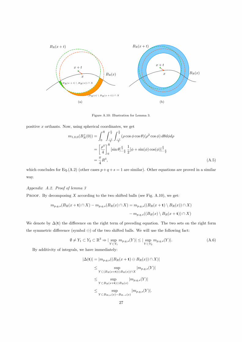
Figure A.10: Illustration for Lemma 3.

positive x orthants. Now, using spherical coordinates, we get

m1,0,0(B+R(0)) =

∫ R

0

∫ π2

−π2

∫ π2

−π2

(ρ cosφ cos θ)(ρ2 cosφ) dθdφdρ

=

[ρ4

4

]R0

[sin θ]π2

−π2

1

2[φ+ sin(φ) cos(φ)]

π2

−π2

=π

4R4, (A.5)

which concludes for Eq.(A.2) (other cases p+ q+ s = 1 are similar). Other equations are proved in a similar

way.

Appendix A.2. Proof of lemma 3

Proof. By decomposing X according to the two shifted balls (see Fig. A.10), we get:

mp,q,s(BR(x+ t) ∩X)−mp,q,s(BR(x) ∩X) = mp,q,s((BR(x+ t) \BR(x)) ∩X)

−mp,q,s((BR(x) \BR(x+ t)) ∩X)

We denote by ∆(t) the difference on the right term of preceding equation. The two sets on the right form

the symmetric difference (symbol ) of the two shifted balls. We will use the following fact:

∅ 6= Y1 ⊂ Y2 ⊂ R3 ⇒ | supY⊂Y1

mp,q,s(Y )| ≤ | supY⊂Y2

mp,q,s(Y )|. (A.6)

By additivity of integrals, we have immediately:

|∆(t)| = |mp,q,s((BR(x+ t)BR(x)) ∩X)|

≤ supY⊂(BR(x+t)BR(x))∩X

|mp,q,s(Y )|

≤ supY⊂BR(x+t)BR(x)

|mp,q,s(Y )|

≤ supY⊂BR+t(x)−BR−t(x)

|mp,q,s(Y )|.

27

In the last row, we cover the symmetric difference of two shifted balls by the difference of two balls of same

center, a kind of spherical shell or annulus in 2D (see Fig. A.10). Although it is a rough upper bound, it

induces the same order of perturbation. We denote this set BR+t(x)−BR−t(x) by HR,t(x).

For zeroth order moment, we use simply the volume of the ball:

supY⊂HR,t(x)

|m0,0,0(Y )| = m0,0,0(HR,t(x))

=4π

3(6R2t+ 2t3) = O(tR2). (A.7)

For first order moment, we translate the shape to the origin, then we use the previous result plus the

fact that the centered 1,0,0-moment is maximized by the x-positive half-ball:

supY⊂HR,t(x)

|m1,0,0(Y )| ≤ supY⊂HR,t(0)

|m1,0,0(Y )|+ |xx||m0,0,0(Y )|

= m1,0,0(B+R+t(0)−B+

R−t(0)) +O(|xx|tR2)

= 2π(R3t+Rt3) +O(|xx|tR2)

= O(tR3) +O(‖x‖tR2). (A.8)

For second order moment, we translate the shape to the origin, then we use the two previous results plus

the fact that the 2,0,0-moment is maximized by the ball:

supY⊂HR,t(x)

|m2,0,0(Y )| ≤ supY⊂HR,t(0)

|m2,0,0(Y )|+ 2|xx||m1,0,0(Y ) + x2x|m0,0,0(Y )|

= m2,0,0(HR,t(0)) + ‖x‖(O(tR3) +O(‖x‖tR2)) + x2xO(tR2)

= O(tR4) +O(‖x‖tR3) +O(‖x‖2tR2) (A.9)

Other moments are proved similarly. �

References

[1] R. Klette, A. Rosenfeld, Digital Geometry: Geometric Methods for Digital Picture Analysis, Series in Computer Graphics

and Geometric Modelin, Morgan Kaufmann, 2004.

[2] D. Coeurjolly, J.-O. Lachaud, T. Roussillon, Digital Geometry Algorithms, Theoretical Foundations and Applications of

Computational Imaging, volume 2 of LNCVB, Springer, 2012, pp. 395–424.

[3] N. Amenta, M. Bern, M. Kamvysselis, A new voronoi-based surface reconstruction algorithm, in: Proceedings of the 25th

annual conference on Computer graphics and interactive techniques, ACM, 1998, pp. 415–421.

[4] Q. Merigot, M. Ovsjanikov, L. Guibas, Voronoi-based curvature and feature estimation from point clouds, Visualization

and Computer Graphics, IEEE Transactions on 17 (2011) 743–756.

[5] T. Surazhsky, E. Magid, O. Soldea, G. Elber, E. Rivlin, A comparison of gaussian and mean curvatures estimation methods

on triangular meshes, in: Robotics and Automation, 2003. Proceedings. ICRA ’03. IEEE International Conference on,

volume 1, 2003, pp. 1021–1026.

28

[6] T. D. Gatzke, C. M. Grimm, Estimating curvature on triangular meshes, International Journal of Shape Modeling 12

(2006) 1–28.

[7] M. Desbrun, A. N. Hirani, M. Leok, J. E. Marsden, Discrete exterior calculus, arXiv preprint math/0508341 (2005).

[8] A. I. Bobenko, Y. B. Suris, Discrete differential geometry: Integrable structure, volume 98, AMS Bookstore, 2008.

[9] D. L. Page, Y. Sun, A. F. Koschan, J. Paik, M. A. Abidi, Normal vector voting: Crease detection and curvature estimation

on large, noisy meshes, Graphical Models 64 (2002) 199–229.

[10] S. Rusinkiewicz, Estimating curvatures and their derivatives on triangle meshes, in: 3D Data Processing, Visualization

and Transmission, 2004. 3DPVT 2004. Proceedings. 2nd International Symposium on, 2004, pp. 486–493.

[11] G. Xu, Convergence analysis of a discretization scheme for gaussian curvature over triangular surfaces, Computer Aided

Geometric Design 23 (2006) 193–207.

[12] D. Cohen-Steiner, J.-M. Morvan, Restricted delaunay triangulations and normal cycle, in: Proceedings of the nine-

teenth annual symposium on Computational geometry, SCG’03, ACM, New York, NY, USA, 2003, pp. 312–321. URL:

http://doi.acm.org/10.1145/777792.777839.

[13] D. Cohen-Steiner, J.-M. Morvan, Second fundamental measure of geometric sets and local approximation of curvatures,

Journal of Differential Geometry 74 (2006) 363–394.

[14] H. Pottmann, J. Wallner, Y. Yang, Y. Lai, S. Hu, Principal curvatures from the integral invariant viewpoint, Computer

Aided Geometric Design 24 (2007) 428–442.

[15] H. Pottmann, J. Wallner, Q. Huang, Y. Yang, Integral invariants for robust geometry processing, Computer Aided

Geometric Design 26 (2009) 37–60.

[16] F. Cazals, M. Pouget, Estimating differential quantities using polynomial fitting of osculating jets, Computer Aided

Geometric Design 22 (2005) 121–146.

[17] P. Alliez, D. Cohen-Steiner, Y. Tong, M. Desbrun, Voronoi-based variational reconstruction of unoriented point sets, in:

Symposium on Geometry processing, volume 7, 2007, pp. 39–48.

[18] Q. Merigot, M. Ovsjanikov, L. Guibas, Robust voronoi-based curvature and feature estimation, in: 2009 SIAM/ACM

Joint Conference on Geometric and Physical Modeling, SPM’09, ACM, New York, NY, USA, 2009, pp. 1–12. URL:

http://doi.acm.org/10.1145/1629255.1629257.

[19] B. Li, R. Schnabel, R. Klein, Z. Cheng, G. Dang, S. Jin, Robust normal estimation for point clouds with sharp features,

Computers & Graphics 34 (2010) 94–106.

[20] A. Boulch, R. Marlet, Fast and robust normal estimation for point clouds with sharp features, Computer Graphics Forum

31 (2012) 1765–1774.

[21] J. Zhang, J. Cao, X. Liu, J. Wang, J. Liu, X. Shi, Point cloud normal estimation via low-rank subspace clustering,

Computers & Graphics 37 (2013) 697–706.

[22] D. Coeurjolly, R. Klette, A comparative evaluation of length estimators of digital curves, IEEE Trans. on Pattern Analysis

and Machine Intelligence 26 (2004) 252–258.

[23] F. de Vieilleville, J.-O. Lachaud, F. Feschet, Maximal digital straight segments and convergence of discrete geometric

estimators, Journal of Mathematical Image and Vision 27 (2007) 471–502.

[24] R. Malgouyres, F. Brunet, S. Fourey, Binomial convolutions and derivatives estimation from noisy discretizations, in:

Discrete Geometry for Computer Imagery, volume 4992 of LNCS, Springer, 2008, pp. 370–379.

[25] H.-A. Esbelin, R. Malgouyres, C. Cartade, Convergence of binomial-based derivative estimation for 2 noisy discretized

curves, Theoretical Computer Science 412 (2011) 4805 – 4813.

[26] L. Provot, Y. Gerard, Estimation of the derivatives of a digital function with a convergent bounded error, in: Discrete

Geometry for Computer Imagery, LNCS, Springer, 2011, pp. 284–295.

[27] T. Roussillon, J.-O. Lachaud, Accurate curvature estimation along digital contours with maximal digital circular arcs, in:

29

Combinatorial Image Analysis, volume 6636, Springer, 2011, pp. 43–55.

[28] B. Kerautret, J.-O. Lachaud, Curvature estimation along noisy digital contours by approximate global optimization,

Pattern Recognition 42 (2009) 2265 – 2278.

[29] A. Lenoir, Fast estimation of mean curvature on the surface of a 3d discrete object, in: E. Ahronovitz, C. Fiorio (Eds.),

Proc. Discrete Geometry for Computer Imagery (DGCI’97), volume 1347 of Lecture Notes in Computer Science, Springer

Berlin Heidelberg, 1997, pp. 175–186. URL: http://dx.doi.org/10.1007/BFb0024839.

[30] S. Fourey, R. Malgouyres, Normals and curvature estimation for digital surfaces based on convolutions, in: Discrete

Geometry for Computer Imagery, LNCS, Springer, 2008, pp. 287–298.

[31] D. Coeurjolly, J. L. Lachaud, J. Levallois, Integral based curvature estimators in digital geometry, in: Discrete Geometry

for Computer Imagery, number 7749 in LNCS, Springer, 2013, pp. 215–227.

[32] DGtal: Digital geometry tools and algorithms library, http://libdgtal.org.

[33] J.-O. Lachaud, Espaces non-euclidiens et analyse d’image : modeles deformables riemanniens et discrets, topologie et

geometrie discrete, Habilitation a diriger des recherches, Universite Bordeaux 1, Talence, France, 2006.

[34] J. W. Bullard, E. J. Garboczi, W. C. Carter, E. R. Fullet, Numerical methods for computing interfacial mean curvature,

Computational materials science 4 (1995) 103–116.

[35] E. Kratzel, Lattice points, volume 33, Springer, 1988.

[36] M. N. Huxley, Area, lattice points and exponential sums, Oxford Science publications, 1996.

[37] R. Klette, J. Zunic, Multigrid convergence of calculated features in image analysis, Journal of Mathematical Imaging and

Vision 13 (2000) 173–191.

[38] E. Kratzel, W. G. Nowak, Lattice points in large convex bodies, Monatshefte fur Mathematik 112 (1991) 61–72.

[39] W. Muller, Lattice points in large convex bodies, Monatshefte fur Mathematik 128 (1999) 315–330.

[40] G. W. Stewart, J.-g. Sun, Matrix perturbation theory (1990).

[41] R. Bhatia, Matrix analysis, volume 169, Springer, 1997.

[42] D. Coeurjolly, S. Miguet, L. Tougne, Discrete curvature based on osculating circle estimation, in: 4th International

Workshop on Visual Form, volume 2059 of Lecture Notes in Computer Science, 2001, pp. 303–312.

[43] CGal: Computational geometry algorithms library, http://www.cgal.org.

[44] T. Kanungo, Document degradation models and a methodology for degradation model validation, Ph.D. thesis, University

of Washington, 1996.

[45] B. Kerautret, J. Lachaud, Meaningful scales detection along digital contours for unsupervised local noise estimation, IEEE

transactions on pattern analysis and machine intelligence 34 (2012) 2379–2392.

30