MULTIFRONTAL SOLUTION OF SPARSE … · MULTIFRONTAL SOLUTION OF SPARSE UNSYMMETRIC MATRICES ARISING FROM SEMICONDUCTOR EQUATIONS ... Here A is a sparse n n matrix and x and b are

CANADIAN APPLIED

MATHEMATICS QUARTERLY

Volume 12, Number 2, Summer 2004

MULTIFRONTAL SOLUTION OF SPARSE

UNSYMMETRIC MATRICES ARISING FROM

SEMICONDUCTOR EQUATIONS

A. EL BOUKILI, A. MADRANE AND R. VAILLANCOURT

ABSTRACT. The multifrontal LU method is implementedto solve drift-diffusion models with large sparse matrices arisingin the simulation and optimization of semiconductor devices.The performance of this method is compared with the LU al-gorithm without multifrontal scheme on different computers inthe case of a realistic double heterojunction transistor.

1 Introduction The solution of large sparse systems of linear equa-tions which occur in solving semiconductor device equations can accountfor as much as 90% of the computational time on industrial-scale prob-lems. Thus, any reduction in the linear system solution time will result ina significant reduction of the total simulation run time. While iterativemethods can be used to solve such systems, their reliability is question-able in the context of drift-diffusion semiconductor equations. In fact,in most applications the matrices arising from the discretization of theseequations are ill conditioned because of the presence and dominance ofadvection terms. For this reason, we focus on direct methods.

In the solution of a large sparse linear system Ax = b the multifrontal,the LU decomposition attempts to minimize fill-ins in the lower and up-per triangular matrices L and U , respectively, in order to reduce runtime. Here A is a sparse n×n matrix and x and b are column vectors oflength n. We recall that the factored system Ax = (LU)x = L(Ux) = b

is solved in two steps. First Ly = b is solved for y by forward sub-stitution and Ux = y is solved for x by backward substitution. In thispaper, we focus on the multifrontal method which is an LU factorization

Partially supported by NSERC of Canada and the Centre de recherchesmathematiques of the Universite de Montreal.

Keywords: sparse matrix, symmetric matrix pattern, multifrontal method, drift-diffusion model, bipolar transistor.

Copyright c©Applied Mathematics Institute, University of Alberta.

137

138 A. EL BOUKILI, A. MADRANE, R. VAILLANCOURT

method which is efficient for a large class of problems. While it may beefficient for unsymmetric and ill-conditioned linear systems, it was infact originally derived for symmetric linear systems [6].

We consider the stationary drift-diffusion model of electron flow in aheterojunction semiconductor device. This model involves a nonlinearPoisson equation and two nonlinear transport equations for electronsand holes, respectively. The stationary problem is first transformed intoan artificial transient nonlinear problem which, in turn, is discretizedinto a nonlinear implicit scheme. At each implicit step, the Newton-Raphson method used for solving nonlinear systems gives rise to largeill-conditioned unsymmetric linear algebraic systems with symmetricpattern. Since these matrices are diagonally dominant, the robustnessand high efficiency of the Multifrontal LU Factorization (MLUF) can betested without using any pivoting.

From several numerical experiments [7] using an unstructured grid[9] (see Figure 3 below) on Dec Alpha 2100, IBM RS6000, HP 900-735and SUN ULTRA’s 1 and 10, the LU factorization algorithm withoutthe multifrontal scheme, which will be named the Standard LU Factor-ization (SLUF), needs 32 hours for a single two-dimensional solution,called characteristic, associated with the currents across the collectorand base contacts as a function of voltage for a realistic Double Hetero-junction Bipolar Transistor (DHBT). On the other hand, MLUF needsonly roughly 13 hours. The most costly and computationally intensivestep is the numerical factorization. The performance of MLUF shows asignificant improvement over SLUF.

The outline of the paper is as follows. Section 2 reviews the basics ofthe multifrontal method. Section 3 introduces the drift-diffusion equa-tions, a corresponding transient problem, and the discretization scheme.Section 4 describes the physical problem of a DHBT characteristic, com-pares the numerical performances of MLUF and SLUF, and presentsthe numerical solution of the two-dimensional problem. A conclusion isdrawn in Section 5.

2 Review of the multifrontal method The multifrontal methodis a generalization of the unifrontal method. It was originally developedfor symmetric matrices. To understand the principle of this method, wefirst present the main idea of the unifrontal method.

2.1 Unifrontal method In a unifrontal scheme [4], [10], the factor-ization proceeds as a sequence of partial factorizations and eliminationson dense submatrices, called frontal matrices. The unifrontal methods

MULTIFRONTAL SOLUTION 139

were originally designed for the solution of finite-element problems [10]and they can be used on assembled systems [4]. For assembled systems,the frontal matrices can be written as

(1)

[

A11 A12

A21 A22

]

,

where all rows are fully summed (that is, there are no further contri-butions to come to the rows in (1)) and the first block column is fullysummed. This means that the pivots can be chosen from anywhere inthe first block column, and, within these columns, numerical pivotingwith arbitrary row interchanges can be accommodated since all rows inthe frontal matrix are fully summed. We assume, without loss of gener-ality, that the pivots that have been chosen are in the square matrix A11

of (1). Then A11 is factored and the Gaussian elimination overwritesA21 and the Schur complement

(2) A22 − A21A−111 A12

is found using dense matrix kernels. The submatrices consisting of therows and columns of the frontal matrix from which pivots have not yetbeen chosen is called the contribution block. In the case above, this is thesame as the Schur complement matrix (2). At the next stage, furtherrows from the original matrix are assembled with the Schur complementto form another frontal matrix.

The entire sequence of frontal matrices is held in the same workingarray. Data movement is limited to assembling rows of the originalmatrix into the frontal matrix, and storing rows and columns as theybecome pivotal. One important advantage of the method is that only thissingle working array needs to reside in memory. A detailed descriptionof frontal methods for assembled matrices is given in [14].

An example is shown in Table 1, where two pivot steps have alreadybeen performed on a 5× 7 frontal matrix (computing the first two rowsof U and columns of L, respectively), the columns are in pivotal order.

Entries in L and U are shown in lower case. Row 6 has just beenassembled into the current 4 × 7 frontal matrix (shown as a solid box).Columns 3 and 4 are now fully summed (a column is fully summedif it has all of its nonzero elements in the frontal matrix) and can beeliminated. After this step, rows 7 and 8 must both be assembled beforecolumns 5 and 6 can be eliminated (the dashed box, a 4 × 6 frontalmatrix containing rows 5 through 8 and columns 5, 6, 7, 8, 9 and 12).The frontal matrix is, of course, stored without the zero columns, that


1 2 3 4 5 6 7 8 9 10 11 12 1 u u u u u 2 l u u u u 3 l l X X X X 4 l l X X X X 5 l l X X X X 6 l l X X X X X X 7 X X X 8 X X X X X X 9 X X X X 10 X X X X X 11 X X X X X X 12 X X

TABLE 1: Two pivot steps already performed on a 5 × 7 frontal matrix.

is, columns 6 and 7 in the dashed box. The dotted box shows the stateof the frontal matrix where the next four pivots can be eliminated. Tofactor the 12×12 sparse matrix in Table 1, a 5×7 (dense) working arrayis sufficient to hold all the frontal matrices.

The unifrontal method works well for matrices with small pattern.But, for matrices with large pattern, the frontal matrices may be verylarge and an unacceptable amount of fill-in may occur.

2.2 Multifrontal method Like the unifrontal method, the multi-frontal method also exploits low-level parallelism and vectorization us-ing the dense matrix kernels on frontal matrices. However, the frontalmatrices in the multifrontal method are generally smaller and denserthan in the unifrontal method.


We are considering the multifrontal method for matrices with a sym-metric sparsity pattern [6]. We perform the following three phases forboth SLUF and MLUF:

• a reordering phase to reduce fill-in by means of the minimum degreealgorithm,

• a symbolic factorization,• a numerical factorization.

Orderings, as by the minimum degree algorithm, tend to reduce fill-inmuch more than profile reduction orderings. The ordering is combinedwith a symbolic analysis to generate an assembly tree in the case of amultifrontal method.

2.3 Multifrontal elimination tree In this subsection, we define theelimination tree based on graph theory and show how it is linked toGaussian elimination. With any sparse symmetric matrix A, we asso-ciate a nondirected graph (V, E), where V is a set of nodes and E is theset of pairs (or edges) expressing the connections between the elementsof V . If n is the order of A, we can label the nodes of the graph byintegers 1, 2, . . ., such that (i, j) ∈ E if and only if aij or aji are nonzero.A sequence of distinct edges (i1, i2), (i2, i3), . . . , (ik−1, ik) is a path. Apath is a cycle if ik = i1 for k > 2. An acyclic graph is a graph withno cycles. If there is a path between any pair of nodes, the graph isconnected. A tree is defined as an acyclic connected graph. A rooted tree

is defined by choosing a node, called root, which gives an orientation tothe tree. For each tree, we can define father nodes, son nodes and leaf

nodes (that is, nodes without sons).A tree associated with Gaussian elimination is called an elimination

tree. Several properties of trees associated with a tree generation algo-rithm are also given in [1]. We recall here two interesting properties.Let A(k) be the modified matrix from rows and columns k to n afterelimination by pivots 1, 2, 3, . . . , k − 1. The essence of the multifrontalapproach to Gaussian elimination is that the elimination operations cor-responding to pivot k can be performed as soon as all the entries in thefirst row and first column of A(k) have been calculated. Its power comesfrom eliminating several variables at a node. Therefore, there is no needto wait until all the entries in A(k) have been computed.

Theorem 2.1 ([1]). The entries which are modified by the sons of node

k are included in a submatrix of A(k) determined by the rows and columns

with nonzeros in row k and column k of A(k).


The entries that are modified by the sons correspond to nonzeros inthe son’s pivot row and column. Theorem 2.1 is equivalent to sayingthat for any son j, say, of node k, the sparsity structure of column j inrows k to n is included in the sparsity structure of column k of A(k).

Corollary 2.1 ([1]). Computation corresponding to tree nodes which

are not ancestors or descendants of one another are independent.

Finite-element problems occur with matrices of the form

(3) A =∑

m

Bm,

where each Bm is the contribution from a single finite element and iszero except in a small number of rows and columns. An example of anassembly tree corresponding to the summation

(4) [[B1 + B2] + [B3 + B4]] + [[B5 + B6] + [B7 + B8]]

is shown in Figure 1.

1 2 3 4 5 6 7 8

9 10 11 12

13 14

15

FIGURE 1: Assembly tree corresponding to bracketing (4).

Using Corollary 2.1, one can exploit the parallelism of the eliminationtree [5].

The multifrontal method associates with each node/edge of the elim-ination tree a process that will exploit the properties of the tree. Thus,


each edge of the elimination tree corresponds to summing contributionsfrom the sons of the node with the rows and columns of the node itself.Consider a node k, say, which is not a leaf node. Then the contributionsof the sons of this node will change the entries in A(k) correspondingto the nonzero entries in column k. We associate with each node k thematrix, called frontal matrix, determined by the nonzero elements in thepivot row and column, respectively, such that the contributions from theprevious eliminations of the descendants of node k can be summed inthe matrix. The outer products from the elimination by pivot k are thenperformed within the frontal matrix of node k.

We refer the reader to [2] for more details.

3 Physical model and discretization schemes

3.1 Drift-diffusion equations We consider the drift-diffusion modelof mobile carrier transport in semiconductor devices [7], [12]. The com-plete system involves a coupled set of three strongly nonlinear partialdifferential equations. The first equation is Poisson’s equation for theelectrostatic potential φ, and the second and third equations are thetransport equations for the quasi-Fermi levels φn and φp for electronsand holes, respectively. The mixed boundary conditions correspond toapplied potential differences on the Ohmic contact portions of the deviceand to insulation in the remaining parts. We have to solve the followingstationary boundary value problem:

(5)

− div[

εr(x)∇φ]

+q

ε0

[

N(x, φ, φn) − P (x, φ, φp) − dop(x)]

= 0 in Ω,

− div[

qµn(x)N(x, φ, φn)∇φn

]

+ q GR(x, φ, φn, φp) = 0 in Ω,

− div[

qµp(x)P (x, φ, φp)∇φp

]

− q GR(x, φ, φn, φp) = 0 in Ω,

φ = g1, φn = φp = g2 on ∂ΩD,

∂φ

∂ν

=∂φn

∂ν

=∂φp

∂ν

= 0 on ∂ΩN .

Here, Ω is a bounded domain in R2, ν is the outward normal vector

to the boundary ∂Ω, and ∂ΩN and ∂ΩD are disjoint parts of ∂Ω suchthat ∂ΩN ∪ ∂ΩD = ∂Ω. The function εr is the semiconductor relative


dielectric permittivity and ε0 is the permittivity of vacuum. The con-stant q is the electron charge and N(x, φ, φn) and P (x, φ, φp) are electronand hole concentrations, respectively. Typical models for these stronglynonlinear functions and the mobilities µn and µp can be found in [7],[11]. The function dop describes the doping profile, and the function GR

is the so-called generation-recombination term which takes the possible“birth” and “death” of positive and negative charges into account. TheShockley-Read-Hall [7] model is used for this term.

To clarify the procedure, we list the steps that will be used in thesolution of the nonlinear stationary system (5) which we write in generalform as

(6) F (u) = 0 on Ω.

When dealing with the solution of such nonlinear systems, a key pointis the choice of iterative methods to compute the solution. For this pur-pose, one often uses variants of Newton-Raphson’s method [7] whosequadratic convergence is achieved only sufficiently near the desired so-lution. Hence, the choice of the initial value is critical. Since in the ap-plications very little a priori knowledge about the solution is available,Newton-Raphson’s method may fail because of poor starting values. Asa remedy, one can use time deformation by transforming (6) into anartificial transient problem of the form

(7)∂u

∂t+ F (u) = 0 on Ω.

The final solution is constructed step by step instead of computing itdirectly. This computing strategy provides a “good” initial guess. Thesolution of our problem is then obtained as the limit solution of anartificial nonstationary problem.

Problem (7) is then discretized in time to yield the system

(8)uk+1 − uk

∆t+ F (uk+1) = 0 on Ω,

which we rewrite as

(9) G(uk+1) = 0 on Ω.


Next, one uses a variational method and looks for a weak solution inthe space X to the problem

(10) (G(uk+1), v) = 0, ∀ v ∈ X.

Spatial discretization of this problem is achieved using a finite elementmethod. This produces the discrete nonlinear system

(11) (G(uk+1h ), vh) = 0, ∀ vh ∈ Xh.

Finally, this problem is solved iteratively by Newton’s method, givingrise to the linear system

(12) G′(ukh)uk+1

h = ukh − G(uk

h),

which is solved by the multifrontal LU decomposition.

3.2 Mixed formulation In the case in hand to approximate the so-lution of (10) we use a mixed finite element (MFE) method [12], [3],based on the dual mixed formulation. The basic idea behind the mixedformulation of (5) is to introduce with the solution (φ, φn, φp) of (5), thedisplacement D and the current densities jn, jp as independent variablesdefined by the expressions

D = εr(x)∇φ,

jn = qµn(x)N(x, φ, φn)∇φn,

jp = qµp(x)P (x, φ, φp)∇φp,

and to derive a suitable variational formulation. In many applications,the flux variables jn and jp, introduced above, are more important thanthe primal variables φ, φn, and φp.

For time discretization, following previous work [7], [8], we use anonlinear implicit scheme with local time steps in which the systemis decoupled into three nonlinear subsystems. Spatial discretization isbased on the Raviart-Thomas finite element of lowest order [7], [13]. Wehave to solve the following problem:


Find (φk+1, Dk+1, φk+1n , jk+1

n , φk+1p , jk+1

p ) such that, in Ω,

(13)

A1(x)φk+1 − φk

δt1− div Dk+1

+q

ε0

[

Nx, φk+1, φk+1n ) − P (x, φk+1, φk+1

p ) − dop(x)]

= 0,

Dk+1 = εr(x)∇φk+1 ,

A2(x)φk+1

n − φkn

δt2− div jk+1

n + q GR(x, φk+1, φk+1n , φk

p) = 0,

jk+1n = qµn(x)N(x, φk+1 , φk+1

n )∇φk+1n ,

A3(x)φk+1

p − φkp

δt3− div jk+1

p − q GR(x, φk+1, φk+1n , φk+1

p ) = 0,

jk+1p = qµp(x)P (x, φk+1 , φk+1

p )∇φk+1p ,

and

(14)

φk+1 = g1, φk+1n = φk+1

p = g2 on ∂ΩD,

Dk+1· ν = jk+1

n · ν = jk+1p · ν = 0 on ∂ΩN ,

where the preconditioners A1, A2 and A3 are uniformly bounded positivefunctions. The local time steps are defined by

δti(x) = A−1i (x)δti, i = 1, 2, 3,

where δti, i = 1, 2, 3, are dimensionless parameters and the time dimen-sion is introduced in A−1

i , i = 1, 2, 3.In solving each nonlinear subsystem by the Newton-Raphson algo-

rithm one obtains a linear system with coefficient matrix M . In the caseof the linearized Poisson equation, M is of the form

M =

[

A Bt

B −C

]

,

where A is associated with a perturbation of the identity operator inL2(Ω)]2, B is associated with the divergence operator and C is associatedwith the source terms. We point out that M is symmetric but not


positive definite since it is associated with a saddle-point problem. Sincethe approximation is of lowest order, the primal variables are constant oneach triangle, so they can be eliminated before the assembly. Thereby,we obtain a positive definite symmetric matrix which can be writtenformally as

A + BtC−1B.

The LLt Cholesky factorization is used to solve this first system.The matrices associated with the linearized transport equations have

the form

M =

[

A Bt + J

B −C

]

,

where J comes from the advection term. If we use, as in the first case,an elimination procedure, we obtain a matrix of the form

A + BtC−1B + JC−1B

which is invertible and diagonally dominant (see [7]), but is neithersymmetric nor positive definite.

For comparison purposes, in Section 4.2 below, the two linear sys-tems associated with the transport equations are solved by means ofthe standard (SLUF) and the multifrontal (MLUF) LU factorizations,respectively.

4 Numerical results In this section, we first describe the struc-ture of a double heterojunction bipolar transistor with collector-up anddefine its computed characteristics and physical objective. Then, wecompare the performance of SLUF and MLUF on single-processorSUN ULTRA’s 1 and 10.

4.1 Double heterojunction bipolar transistor with collector-up

We consider a realistic device whose structure is shown in Figure 2. Thisdevice could work as a high-power amplifier. For the present simulation,the sub-emitter is omitted.

The materials and the doping values were provided by Thomson Lab-oratory [7]. Let VC , VB and VE be the applied voltage at the collector,base, and emitter contacts, respectively. The characteristic is associatedwith the values of the current IC across the collector contact and thecurrent IB across the base contact, as VC and VB increase from 0.2 to1.3 volts. The applied voltage VE = 0 in our case. The mesh for thepresent simulation is presented in Figure 3.


Sub-Emitter

Emitter

SpacerBase

Collector

Cap

FIGURE 2: Double heterojunction bipolar transistor with collector-up.

FIGURE 3: Mesh containing 11347 elements, 17200 edges, and 5854vertices.

4.2 Comparison of SLUF and MLUF In this subsection, we com-pare the performance of the SLUF and MLUF methods. These twomethods use the same storage strategy, the minimum degree algorithmand symbolic factorization. The two phases (reordering and symbolicfactorization) are not really time consuming and are performed onlyonce. Since no pivoting is used and hence the sparsity is preserved,then there is no need to perform these two preprocessing steps morethan once. We are only comparing the overall run time to perform thenumerical factorization (FACTOR) and to solve a single linear system(SOLVE) as presented in Table 3.

The matrices in this problem are of order 17,200. The number ofnonzero entries after factorization and the number of floating-point op-


erations (flops) needed for the LU factorization step using both SLUF

and MLUF are listed in Table 2.

SLUF MLUF

Number of nonzero entries 2,348,962 593,204Number of megaflops 375 20

TABLE 2: Number of nonzero entries and megaflops with the variableband and the multifrontal methods.

When 0.2 volts are applied to the structure, 76 LU factorizationsare needed to solve the nonlinear system associated with the transportelectron equation. Table 3 presents the run times for this number ofdouble-precision factorizations on SUN ULTRA’s 1 and 10 whose CPUand RAM specifications are presented in Table 4.

SUN SLUF MLUF

FACTOR ULTRA 1 4415.00 s 136.07 sULTRA 10 1602.06 s 47.38 s

SOLVE ULTRA 1 237.24 s 18.66 sULTRA 10 88.15 s 5.58 s

TABLE 3: Performance of the standard and the multifrontal methodsfor ULTRA’s 1 and 10.

ULTRA 1 ULTRA 10CPU 135 MHertz 440 MHertzRAM 64 MBytes 1 GByte

TABLE 4: Specifications of uniprocessor SUN ULTRA’s 1 and 10.

Note that the results listed in Table 3 are obtained without pivoting,because it is known, a priori that the matrices are diagonally dominant.

The total run time (CPU on an ULTRA 10) of our program usingSLUF and MLUF to compute one DHBT-characteristic is given in


Y

X

0 0.25 0.50 0.75 1.0

0

0.5

1.0

1,5

2.0

0

5

10Z

0

5

10

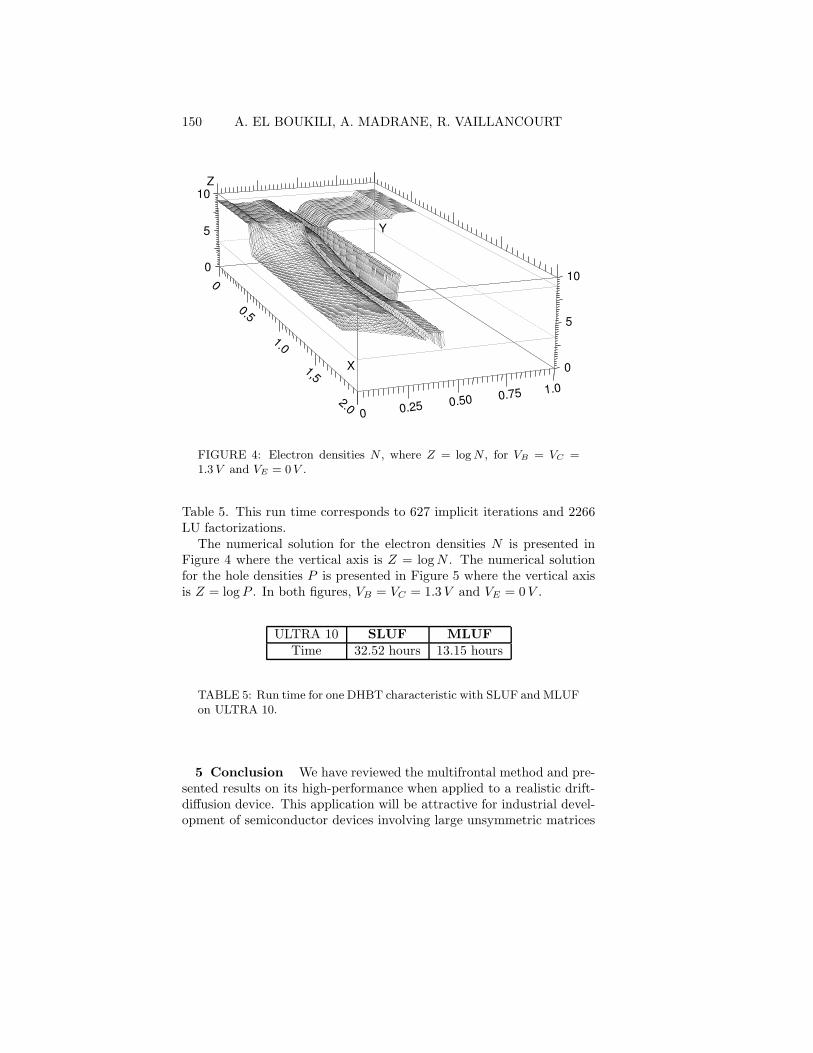
FIGURE 4: Electron densities N , where Z = log N , for VB = VC =1.3 V and VE = 0 V .

Table 5. This run time corresponds to 627 implicit iterations and 2266LU factorizations.

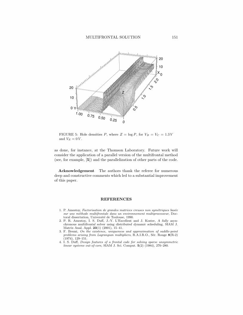
The numerical solution for the electron densities N is presented inFigure 4 where the vertical axis is Z = log N . The numerical solutionfor the hole densities P is presented in Figure 5 where the vertical axisis Z = log P . In both figures, VB = VC = 1.3 V and VE = 0 V .

ULTRA 10 SLUF MLUF

Time 32.52 hours 13.15 hours

TABLE 5: Run time for one DHBT characteristic with SLUF and MLUFon ULTRA 10.

5 Conclusion We have reviewed the multifrontal method and pre-sented results on its high-performance when applied to a realistic drift-diffusion device. This application will be attractive for industrial devel-opment of semiconductor devices involving large unsymmetric matrices


1.00 0.75 0.50 0.25 0

0.5

1.0

1.5

2.0

20

10

0 Y

20

10

0X

Z

FIGURE 5: Hole densities P , where Z = log P , for VB = VC = 1.3 V

and VE = 0 V .

as done, for instance, at the Thomson Laboratory. Future work willconsider the application of a parallel version of the multifrontal method(see, for example, [5]) and the parallelization of other parts of the code.

Acknowledgement The authors thank the referee for numerousdeep and constructive comments which led to a substantial improvementof this paper.

REFERENCES

1. P. Amestoy, Factorisation de grandes matrices creuses non symetriques baseesur une methode multifrontale dans un environnement multiprocesseur, Doc-toral dissertation, Universite de Toulouse, 1990.

2. P. R. Amestoy, I. S. Duff, J.-Y. L’Excellent and J. Koster, A fully asyn-chronous multifrontal solver using distributed dynamic scheduling, SIAM J.Matrix Anal. Appl. 23(1) (2001), 15–41.

3. F. Brezzi, On the existence, uniqueness and approximation of saddle-pointproblems arising from Lagrangian multipliers, R.A.I.R.O., Ser. Rouge 8(R-2)(1974), 129–151.

4. I. S. Duff, Design features of a frontal code for solving sparse unsymmetriclinear systems out-of-core, SIAM J. Sci. Comput. 5(2) (1984), 270–280.


5. I. S. Duff, N. I. M. Gould, M. Lescrenier and J. K. Reid, The multifrontalmethod in a parallel environment, in : Reliable Numerical Computation (M. G.Cox and S. Hammarling, eds.), Oxford, Oxford University Press, 1990, 93–111.

6. I. S. Duff and J. K. Reid, The multifrontal solution of indefinite sparse sym-metric linear systems, ACM Trans. Math. Software 9 (1983), 302–325.

7. A. El Boukili, Analyse mathematique et simulation numerique bidimension-nelle des equations des semiconducteurs par l’approche elements finis mixtes,Doctoral dissertation, Universite Paris 6, 1995.

8. A. El Boukili, Arclength continuation method and its application to 2D drift-diffusion semiconductor equations with mixed finite element approach, Compel15(4) (1996), 36–47.

9. A. El Boukili, A. Madrane and R. Vaillancourt, Unstructered grid adaptationfor convection-dominated semiconductor equations, Can. Appl. Math. Quar-terly, 10(4) (Winter 2002), 447–472.

10. B. M. Irons, A frontal solution program for finite element analysis, Internat.J. Numer. Methods Eng. 2 (1970), 5–32.

11. P. A. Markowich, The Stationary Semiconductor Device Equations, in: Com-putational Microelectronics, Springer-Verlag, Vienna, 1986.

12. M. S. Mock, Analysis of Mathematical Models of Semiconductors Devices,Boole Press, Dublin, 1983.

13. P.-A. Raviart and J.-M. Thomas, A mixed finite element method for 2nd orderelliptic problems, in: I. Gal ligani and E. Magenes eds., Mathematical Aspectsof Finite Element Methods, Lecture Notes in Math., Vol. 606, Springer-Verlag,Berlin, 1977, 292–315.

14. S. E. Zitney, Sparse matrix methods for chemical process separation calcula-tions on supercomputers In Proc. Superecomputing 92, Minneapolis MN, Nov.1992, IEEE Computer Society Press, 414–423.

Corresponding author:

R. Vaillancourt

Department of Mathematics and Statistics, University of Ottawa, Ottawa,

Canada K1N 6N5

E-mail address: [email protected]

Documents

MULTIFRONTAL SOLUTION OF SPARSE … · MULTIFRONTAL SOLUTION OF SPARSE UNSYMMETRIC MATRICES ARISING FROM SEMICONDUCTOR EQUATIONS ... Here A is a sparse n n matrix and x and b are