Multifamily Central DHW and Solar Water Heating · Multifamily Central DHW and Solar Water Heating 2013 California Building Energy Efficiency Standards California Utilities Statewide

CODES AND STANDARDS ENHANCEMENT INITIATIVE (CASE)

Multifamily Central DHW and Solar Water

Heating

2013 California Building Energy Efficiency Standards

California Utilities Statewide Codes and Standards Team October 2011

This report was prepared by the California Statewide Utility Codes and Standards Program and funded by the California utility customers under the

auspices of the California Public Utilities Commission.

Copyright 2011 Pacific Gas and Electric Company, Southern California Edison, SoCalGas, SDG&E.

All rights reserved, except that this document may be used, copied, and distributed without modification.

Neither PG&E, SCE, SoCalGas, SDG&E, nor any of its employees makes any warranty, express of implied; or assumes any legal liability or

responsibility for the accuracy, completeness or usefulness of any data, information, method, product, policy or process disclosed in this document;

or represents that its use will not infringe any privately-owned rights including, but not limited to, patents, trademarks or copyrights

Page 2

2013 California Building Energy Efficiency Standards October 2011

Table of Contents

CODES AND STANDARDS ENHANCEMENT INITIATIVE (CASE) ....................... 1

1. Purpose ........................................................................................................................ 7

2. Overview ....................................................................................................................... 8

3. Methodology............................................................................................................... 18

3.1 Methodology for Multifamily DHW Improvements ................................................................18

3.1.1 Data Collection ..................................................................................................................18

3.1.2 Energy Savings Modeling ..................................................................................................20

3.1.3 Cost Analysis .....................................................................................................................23

3.1.4 Cost-Effectiveness Analysis ..............................................................................................24

3.1.5 Statewide Savings Estimates ..............................................................................................24

3.1.6 Stakeholder Meeting Process .............................................................................................24

3.2 Methodology for Multifamily Solar Water Heating .................................................................25

3.2.1 Data Collection ..................................................................................................................25

3.2.2 Energy Savings Simulation ................................................................................................26

3.2.3 Simulation Approaches ......................................................................................................29

3.2.4 Cost Analysis .....................................................................................................................31

3.2.5 Cost Effectiveness Analysis ...............................................................................................32

3.2.6 Statewide Savings Estimates ..............................................................................................33

3.2.7 Stakeholder Meeting Process .............................................................................................33

4. Analysis and Results ................................................................................................. 35

4.1 Analysis and Results for Recirculation Loop Improvements ...................................................35

4.1.1 Data Collection/Market Study ...........................................................................................35

4.1.2 Energy Savings Analysis ...................................................................................................42

4.1.3 Energy Savings Results......................................................................................................48

4.1.4 Cost Analysis .....................................................................................................................49

4.2 Analysis and Results for Solar Water Heating .........................................................................50

4.2.1 Solar Water Heating Technology.......................................................................................50

4.2.2 Current Title 24 Requirements...........................................................................................51

4.2.3 Market Condition of Solar Water Heating Systems ..........................................................52

4.2.4 Existing Solar Ready Regulations and Voluntary Codes ..................................................55

4.2.5 Energy Savings ..................................................................................................................58

Page 3


4.2.6 Cost and Cost Savings .......................................................................................................68

4.3 Cost-Effectiveness Analysis .....................................................................................................72

4.3.1 LCC Results of Demand Control and Optimal Design Implementation (Level 1 and 2) ..73

4.3.2 LCC Results of the Combined Package (Level 3) .............................................................73

4.3.3 Cost Effective Solar Savings Fractions..............................................................................76

4.3.4 Solar Water Heating Ready Measure Cost Effective Adoption Rates ...............................80

4.4 Statewide Savings Estimates ....................................................................................................82

5. Recommended Language for the Standards Document, ACM Manuals, and the Reference Appendices ....................................................................................................... 85

5.1 Section 101(b)...........................................................................................................................85

5.2 Section 151(f) 8C......................................................................................................................85

5.3 Section 113(c)2 .........................................................................................................................86

5.4 Section 150(n)...........................................................................................................................86

5.5 Reference Appendix 9.1.1 ........................................................................................................87

6. Bibliography and Other Research ............................................................................ 88

7. Appendices ................................................................................................................ 89

7.1 Recirculation Loop Model Validation Results .........................................................................89

7.2 Screenshots of the Recirculation Model ...................................................................................91

7.3 Solar Water Heating Online Survey Instrument .......................................................................93

7.4 Example of Solar Water Heating Ready Ordinances ...............................................................93

7.5 Energy Saving: Solar Water Heating Simulation Results ........................................................93

7.5.1 Comparison between Climate Zones (high-rise prototype) ...............................................93

7.5.2 Comparison between Various Configurations ...................................................................94

7.6 System Assumptions from CSI-Thermal Incentive Calculator Documentation ....................102

7.7 Evolution of Recommended Code Language .........................................................................102

7.7.1 First Version.....................................................................................................................102

7.7.2 Second Version ................................................................................................................104

7.7.3 CalSEIA’s Written Comment ..........................................................................................106

7.7.4 Third Version ...................................................................................................................106

7.8 Residential Construction Forecast Details ..............................................................................108

7.9 Non-Residential Construction Forecast details ......................................................................111

7.9.1 Citation .............................................................................................................................112

Page 4


7.10 Pipe Sizing Calculation .......................................................................................................113

7.11 Environmental Impact .........................................................................................................116

Table of Figures

Figure 1. Low-Rise Multifamily Prototype Energy Savings ................................................................ 10

Figure 2. High-Rise Multifamily Prototype Energy Savings ............................................................... 11

Figure 3. Annual Statewide Energy Savings ........................................................................................ 12

Figure 4. Low-rise Building Prototype LCC Results............................................................................ 15

Figure 5. High-rise Building Prototype LCC Results ........................................................................... 16

Figure 6. Central DHW System Energy Performance .......................................................................... 19

Figure 7. Building Prototype Characteristics ........................................................................................ 21

Figure 8. Low-rise Prototype Recirculation Piping .............................................................................. 21

Figure 9. High-rise Prototype Recirculation Piping ............................................................................. 22

Figure 10. Distribution Network Characteristics .................................................................................. 22

Figure 11. Recirculation Loop Layout – Low-rise ............................................................................... 23

Figure 12. Recirculation Loop Pipe Layout – High-rise....................................................................... 23

Figure 13. Comparison between Various TRNSYS-based Tools ......................................................... 28

Figure 14. Performance Base Simluation Inputs .................................................................................. 30

Figure 15. Permutation Simulation Phase I Inputs ............................................................................... 31

Figure 16. Permutation Simulation Phase II Inputs .............................................................................. 31

Figure 17. Multifamily DHW System Performance Statistics.............................................................. 36

Figure 18. Example of Monitored Temperature Modulation Operation............................................... 37

Figure 19. Example of Monitored Demand Control Operation ............................................................ 38

Figure 20. Summary of Recirculation Loop Systems .......................................................................... 40

Figure 21. Site 1 - SFD ......................................................................................................................... 41

Figure 22. Site 2 - SAM ........................................................................................................................ 41

Figure 23. Site 3 - SFF .......................................................................................................................... 42

Figure 24. Site 4 - SFH ......................................................................................................................... 42

Figure 25. Control Schedule for Temperature Modulation and Continuous Monitoring (Part 1) ........ 45

Figure 26. Control Schedule for Temperature Modulation and Continuous Monitoring (Part 2) ........ 46

Figure 27. Control Schedule for Demand Control (Part 1) ................................................................... 47

Page 5


Figure 28. Control Schedule for Demand Control (Part 2) ................................................................... 48

Figure 29. Control Energy Savings ....................................................................................................... 49

Figure 30. Copper Piping Type L Cost ($/ft) for different pipe diameter ............................................ 50

Figure 31. Recirculation Configuration Cost ........................................................................................ 50

Figure 32. Domestic Shipment of Solar Thermal Collectors in 2009 (in 1000s of ft2) ........................ 52

Figure 33. Solar Water Heating Penetration Rate in Apartments/Condos............................................ 53

Figure 34. System Configuration Breakcdown ..................................................................................... 54

Figure 35. Online Survey Results: Market Barriers Ranking ............................................................... 55

Figure 36. Energy Savings and Solar Fractions of Base Performance Runs - Low-Rise Multifamily

Prototype, Active Glycol with External HX System ..................................................................... 59

Figure 37. Cold Water Inlet Tempratures by Climate Zone ................................................................. 59

Figure 38. Solar Savings Fractions for Various Configurations ........................................................... 60

Figure 39. Percentage Differences in Solar Savings Fractions ............................................................. 61

Figure 40. Energy Savings and Solar Savings Fractions with Varying Parameter Sizings - Active

Glycol (external HX), CZ 10, Low-rise Prototype......................................................................... 63

Figure 41. Solar Savings Fractions vs. Collector Sizing Ratio ............................................................. 64

Figure 42. Solar Orientation Factors vs. Collector Tilt and Orientation - CZ 1, Single Family House 65

Figure 43. Solar Savings Fractions over a Completel Range of Collector Sizing Ratio - Various

Climate Zones, Low-rise Prototype ............................................................................................... 66

Figure 44. Energy Savings vs. Collector Sizing Ratio w/ Base and Reach TDV - CZ 10, Low-rise and

High-rise Prototypes ....................................................................................................................... 67

Figure 45. Solar Savings Fraction vs. Collector Sizing Ratio - High Solar Insolation case: CZ 10,

Low-rise Prototype ......................................................................................................................... 68

Figure 46. Installed System Costs vs. Collector Area .......................................................................... 69

Figure 47. Component Life Expectancy ............................................................................................... 70

Figure 48. PV of Maintenance Costs at Various Collector Sizing Ratios - Low-rise and High-rise

Prototypes ....................................................................................................................................... 71

Figure 49. Solar Water Heating Ready Cost and Cost Savings per Building - Low-rise and High-rise

........................................................................................................................................................ 72

Figure 50. Level 1 and Level 2 LCC – Average Over All Climate Zones ........................................... 73

Figure 51. Level 3 Improvement LCC - CZ 10 .................................................................................... 74

Figure 52. LCC of All Three Proposed Requirement Levels - CZ 10 .................................................. 75

Figure 53. Highest Cost Effective Solar Savings Fractions .................................................................. 76

Figure 54. Costs for Alternative Compliance Equipment ..................................................................... 77

Page 6


Figure 55. Alternative Compliance Method to Installing Solar Water Heating ................................... 78

Figure 56. Collector Area in % Total of Building Footprint Calculation (SSF = 50%) ....................... 79

Figure 57. Roof Area for Solar Collectors (SSF = 50%) ...................................................................... 79

Figure 58. Cost Effective Adoption Rates for Ready Measure ............................................................. 80

Figure 59. Statewide Energy Savings: Low-rise MF prototype ........................................................... 82

Figure 60. Statewide Energy Savings: High-rise MF prototype ........................................................... 83

Figure 61. Statewide Energy Savings: Motels/Hotels .......................................................................... 84

Figure 62. Total Statewide Energy Savings .......................................................................................... 84

Page 7


1. Purpose

This Codes and Standards Enhancement (CASE) report regards potential changes to the 2008

California Building Energy Efficiency Standards for adoption into the 2013 Standards. It proposes

changes in mandatory and prescriptive requirements for multifamily buildings with central domestic

hot water features and summarizes the research supporting these proposed requirements.

Page 8


2. Overview

a. Measure

Title

Multifamily Central Domestic Hot Water (DHW) and Solar Water Heating

b.

Description

This proposal adds the prescriptive requirement of demand control for DHW system

serving multiple dwellings with recirculation loops and revises the existing mandatory

timer control requirement. This proposal adds the prescriptive requirement on DHW

system with recirculation loops serving multiple dwellings to have (at least) two

separate recirculation loops, each serving a portion of the building.

This proposal adds a prescriptive requirement for multifamily buildings with central

DHW systems with recirculation loops to install a solar water heating system with

prescribed minimum solar savings fraction (% water heating budget) by climate zone.

The proposal adds a mandatory requirement for all multifamily buildings to be

designed ready for future installation of solar water heating systems if they otherwise

do not have solar water heating systems installed at the time of building design and

construction.

c. Type of

Change

Mandatory Measure – This proposal will add requirements in Section 150(n) for

multifamily buildings to be solar water heating ready.

This proposal recommend the revision of mandatory requirement of timer control of

DHW recirculation loops in Section 113(c)2.

Prescriptive Requirement – This proposal adds the following requirements to

Section 151(f)8c:

Multifamily building DHW systems with recirculation loops shall have

1. demand controls, and

2. (at least) two recirculation loops, each serving half of the building, and,.

3. a solar water heating system with a minimum solar savings fraction by

climate zone in the following table.

CZ 1 2 3 4 5 6 7 8 9 10 11 12 13 14 15 16

SSF 0.20 0.35

Compliance Option - No change proposed. For the proposed prescriptive

requirements, the CASE study demonstrates the feasibility and cost-effectiveness of

alternative compliance methods.

Modeling – No change proposed by this CASE study. The Water and Space Heating

CASE study proposes new algorithms for multi-family central DHW system and

controls.

Page 9


d. Energy

Benefits

The energy benefits of the measures proposed for 2013 Standards relative to 2008

Standards are presented in this section. The prototype buildings used to arrive at these

energy savings are described in the following table:

Building Type Low-rise High-rise

Building

Characteristics

Number of Floors 2 4

Number of Units 44 88

Conditioned Floor

Area/Unit (sf) 870

Floor to Ceiling Height (ft) 10

Figure 1 and Figure 2 show the per prototype energy savings resulting from proposed

prescriptive measures for the low-rise and high-rise prototype buildings for each of

the 16 climate zones. The last columns of the table also display the per square footage

conditioned floor area (CFA) savings for the prototype buildings.

Page 10


Figure 1. Low-Rise Multifamily Prototype Energy Savings

Climate

Zone Electricity Savings

Natural Gas

Savings

TDV

Electrici

ty

Savings

TDV

Gas

Savings

PV of Energy Cost

Savings

kwh/yr

kWh/yr

per ft2

CFA

Therms

/yr

Therms/

yr per

ft2 CFA

TDV

kBTU

TDV

kBTU PV$

PV$

per ft2

CFA

1 (614) (0.016) 2,271 0.059 (9,727) 356,947 $ 63,504 $ 1.66

2 (767) (0.020) 2,230 0.058 (15,941) 350,441 $ 63,453 $ 1.66

3 (790) (0.021) 2,229 0.058 (14,140) 349,995 $ 63,064 $ 1.65

4 (827) (0.022) 2,213 0.058 (15,973) 348,024 $ 63,040 $ 1.65

5 (775) (0.020) 2,311 0.060 (13,800) 364,895 $ 65,586 $ 1.71

6 (828) (0.022) 2,165 0.057 (15,483) 341,903 $ 61,895 $ 1.62

7 (838) (0.022) 2,173 0.057 (15,758) 343,915 $ 62,291 $ 1.63

8 (853) (0.022) 2,170 0.057 (16,633) 342,558 $ 62,208 $ 1.63

9 (859) (0.022) 2,161 0.056 (17,199) 341,274 $ 62,083 $ 1.62

10 (526) (0.014) 2,758 0.072 (8,472) 435,220 $ 76,842 $ 2.01

11 (496) (0.013) 2,812 0.073 (8,147) 438,204 $ 77,303 $ 2.02

12 (442) (0.012) 2,838 0.074 (6,435) 440,594 $ 77,420 $ 2.02

13 (523) (0.014) 2,753 0.072 (9,136) 428,175 $ 75,737 $ 1.98

14 (535) (0.014) 2,802 0.073 (9,101) 442,269 $ 78,172 $ 2.04

15 (642) (0.017) 2,566 0.067 (11,884) 406,674 $ 72,489 $ 1.89

16 (371) (0.010) 3,016 0.079 (4,667) 470,337 $ 82,265 $ 2.15

Page 11


Figure 2. High-Rise Multifamily Prototype Energy Savings

The Time Dependent Valuation (TDV) method emphasizes the energy savings

benefits during peak demands, especially electricity peak demands. The application of

a demand control system reduces the pump electric energy use by eliminating the

constant pump operation throughout the day. Optimal recirculation loop design, solar

water heating, and solar water heating ready all generate natural gas savings, not

electric energy savings. There is actually increased electric energy consumption due

to pumps for the solar water heating system operation, as indicated by the negative

electric savings.

The assumptions and calculations used to derive the energy and demand savings for

prototype buildings are documented in Section 2 “Methodology” and Section 3

“Analysis and Results.”

The annual statewide energy savings from the proposed measures are displayed in

Figure 3 below.

Climate

Zone

Electricity

Savings

Natural Gas

Savings

TDV

Electricit

y Savings

TDV

Gas

Savings

PV of Energy Cost

Savings

kwh/yr

kWh/yr

per ft2

CFA

Therms

/yr

Therms/

yr per

ft2 CFA

TDV

kBTU

TDV

kBTU PV$

PV$

per ft2

CFA

1 (952) (0.012) 3,716 0.049 (16,095) 597,949 $ 94,557 $ 1.24

2 (1,261) (0.016) 3,635 0.047 (28,854) 584,823 $ 94,500 $ 1.23

3 (1,320) (0.017) 3,631 0.047 (25,362) 584,013 $ 93,838 $ 1.23

4 (1,397) (0.018) 3,599 0.047 (29,150) 580,065 $ 93,813 $ 1.23

5 (1,290) (0.017) 3,796 0.050 (24,655) 613,756 $ 98,309 $ 1.28

6 (1,406) (0.018) 3,503 0.046 (28,291) 568,138 $ 91,844 $ 1.20

7 (1,427) (0.019) 3,521 0.046 (28,862) 572,158 $ 92,551 $ 1.21

8 (1,458) (0.019) 3,513 0.046 (30,682) 569,456 $ 92,415 $ 1.21

9 (1,471) (0.019) 3,495 0.046 (31,857) 566,890 $ 92,201 $ 1.20

10 (796) (0.010) 4,689 0.061 (14,843) 752,548 $ 118,171 $ 1.54

11 (736) (0.010) 4,797 0.063 (13,557) 760,336 $ 119,172 $ 1.56

12 (628) (0.008) 4,850 0.063 (10,083) 765,126 $ 119,375 $ 1.56

13 (794) (0.010) 4,680 0.061 (15,620) 740,320 $ 116,407 $ 1.52

14 (812) (0.011) 4,778 0.062 (16,059) 766,547 $ 120,514 $ 1.57

15 (1,031) (0.013) 4,305 0.056 (21,630) 695,762 $ 110,471 $ 1.44

16 (483) (0.006) 5,206 0.068 (6,498) 824,555 $ 127,974 $ 1.67

Page 12


Building Type Electric

Savings

Gas

Savings

TDV Energy

Savings

(GWh/yr) (MMT/yr) (MBtu/yr)

Low-Rise MF (0.23) 0.87 132,299

High-Rise MF (0.20) 0.60 92,570

Hotel/Motel (0.16) 0.52 78,816

Total (0.59) 1.98 303,685

Figure 3. Annual Statewide Energy Savings

e. Non-

Energy

Benefits

The solar water heating ready measures would substantially reduce the cost of future

installation of solar hot water heating systems. Prescriptive requirements for installing

solar water heating with minimum solar savings fraction and making buildings solar

water heating ready could potentially result in increased property valuation. These

could seem attractive to building owners/operators and tenants interested in utilizing

renewable energy sources.

f. Environ-

mental

Impact

Material use impact from the proposed measures are summarized below. Detailed

calculation can be found in Section 7.11.

Mercury

(lb)

Lead

(lb)

Copper

(lb)

Steel

(lb)

Plastic

(lb)

Glass

(lb)

Aluminum

(lb)

per

low-rise

building

0.01 0.05 272 1922 99 708 191

per

high-rise

building

0.01 0.05 583 3842 185 1356 366

Statewide 10 48 353,356 2,411,079 120,287 869,882 234,645

Water Consumption:

On-Site (Not at the Power plant) Water Savings

(or Increase)

(Gallons/Year)

Per Prototype Building NC

1. For description of prototype buildings refer to Section 3.2.2 below.

Water Quality Impacts: NA

g.

Technology

Measures

Measure Availability:

Demand control products for DHW recirculation are widely available in the market

and ready to meet the increased demand generated by the proposed code change.

Manufacturers include Enovative Group, Taco, Uponor and Advanced Conservation

Technology Distribution.

Design and implementation of optimal recirculation systems for at least two

Page 13


recirculation loops in a building is common practice, so the proposed requirement will

not result in significant change in market practice.

Solar water heating is a mature technology with established product availability and

distribution channels. Since its inception in 1980, the Sola Ratings and Certification

Corporation now has over 400 collector products rated from 155 manufacturers in its

OG-100 collector database. The Energy Information Administration (EIA) Solar

Thermal Collector Manufacturers Report shows that California accounts for over a

quarter of domestic solar thermal collectors (3.5 million sqft) shipped in 2009.

Further, the five largest manufacturers account for 79% of market share.

Industry stakeholders have suggested that there is room for improvement in terms of

consistent design strategy for multifamily solar water heating systems. They also

identified lack of trained installers as one of the major market barriers. However, both

these issues are expected to be addressed with the recently started California Solar

Initiative (CSI)-Thermal incentive program. By 2014, this program will greatly

increase solar industry design experiences and work force to ensure successful

implementation of the proposed code changes.

Useful Life, Persistence, and Maintenance:

Demand control equipment is assumed to have a useful life of 15 year with no

maintenance needs.

Useful life of Optimal design is assumed to be 30 years as energy savings benefits

associated will persist through the entire building life.

The solar water heating system components and maintenance/replacement schedule

are shown below.

Component

Life

Expectancy

(yr)

Implementations

during 30 year

Building Life

Collector 20 1.5

Solar Tank 15 2

Motor and Pump 10 3

Controller 20 1.5

Heat Transfer Fluid Check 1 20

Heat Transfer Fluid Check & Replacement 3 10

h.

Performance

Verification

of the

Proposed

Measure

Field verification of the installation of demand control equipment, implementation of

optimal design and installation of solar water heating systems will be required during

building inspection by building officials. Performance verification of solar water

heating system installation is a more specialized task and shall be performed by

system design/contractors.

Page 14


Page 15


i. Cost Effectiveness

Climate

Zone

Measure

Life

Additional

Costs1– Current

Measure Costs

(Relative to

Basecase)

PV of Additional

Maintenance Costs

(Savings) (Relative

to Basecase)

PV of Energy

Cost Savings –

Per Proto

Building (PV$)

LCC Per

Prototype

Building

Solar

Savings

Fraction

(Years) ($) (PV$) (PV$) ($) (%)

1 30 $ 43,072 $ 12,792 $ 63,504 $ (7,639) 20%

2 30 $ 35,428 $ 11,109 $ 63,453 $ (16,916) 20%

3 30 $ 30,775 $ 5,496 $ 63,064 $ (22,205) 20%

4 30 $ 29,736 $ 5,350 $ 63,040 $ (23,447) 20%

5 30 $ 30,775 $ 5,496 $ 65,586 $ (24,726) 20%

6 30 $ 26,579 $ 4,907 $ 61,895 $ (26,156) 20%

7 30 $ 26,579 $ 4,907 $ 62,291 $ (26,552) 20%

8 30 $ 27,106 $ 4,981 $ 62,208 $ (25,825) 20%

9 30 $ 27,104 $ 4,981 $ 62,083 $ (25,702) 20%

10 30 $ 42,179 $ 7,096 $ 76,842 $ (22,068) 35%

11 30 $ 47,588 $ 7,856 $ 77,303 $ (15,929) 35%

12 30 $ 48,600 $ 7,998 $ 77,420 $ (14,811) 35%

13 30 $ 48,595 $ 7,997 $ 75,737 $ (13,134) 35%

14 30 $ 40,780 $ 6,900 $ 78,172 $ (25,104) 35%

15 30 $ 38,599 $ 6,594 $ 72,489 $ (22,082) 35%

16 30 $ 49,629 $ 8,142 $ 82,265 $ (18,400) 35%

Figure 4. Low-rise Building Prototype LCC Results

Climat

e

Zone

Measure

Life

(Year)

Additional

Costs1– Current

Measure Costs

(Relative to

Basecase)

PV of Additional

Maintenance Costs

(Savings) (Relative

to Basecase)

PV of Energy

Cost Savings

– Per Proto

Building

(PV$)

LCC Per

Prototype

Building

Solar

Savings

Fraction

1 30 $ 83,202 $ 26,222 $ 94,557 $ 14,868 20%

2 30 $ 67,797 $ 22,881 $ 94,500 $ (3,822) 20%

3 30 $ 57,497 $ 10,400 $ 93,838 $ (15,693) 20%

4 30 $ 55,419 $ 10,080 $ 93,813 $ (18,198) 20%

5 30 $ 57,497 $ 10,400 $ 98,309 $ (20,165) 20%

6 30 $ 48,397 $ 9,000 $ 91,844 $ (24,774) 20%

Page 16


7 30 $ 48,397 $ 9,000 $ 92,551 $ (25,481) 20%

8 30 $ 49,488 $ 9,168 $ 92,415 $ (24,018) 20%

9 30 $ 49,484 $ 9,167 $ 92,201 $ (23,808) 20%

10 30 $ 79,935 $ 13,851 $ 118,171 $ (12,722) 35%

11 30 $ 90,972 $ 15,548 $ 119,172 $ (292) 35%

12 30 $ 92,961 $ 15,854 $ 119,375 $ 1,926 35%

13 30 $ 92,953 $ 15,853 $ 116,407 $ 4,882 35%

14 30 $ 77,111 $ 13,416 $ 120,514 $ (18,501) 35%

15 30 $ 72,775 $ 12,749 $ 110,471 $ (13,735) 35%

16 30 $ 94,984 $ 16,165 $ 127,974 $ (4,212) 35%

Figure 5. High-rise Building Prototype LCC Results

j. Analysis

Tools

The current Title 24 ACM and building simulation tools does not include the

necessary algorithms to model demand control and recirculation loop designs of

multi-family DHW systems. This CASE study used a recirculation loop model,

which was developed based on the PIER studies on multi-family DHW distribution

system and was validated by field monitoring data, to analyze energy savings by

control technologies and optimal recirculation loop designs.

CEC’s version of F-chart can be used to quantify energy savings in terms of solar

savings fractions resulting from the installation of solar water heating systems. The

CEC is in the process of adding hourly calculation capability to the tool to enable

more accurate assessment of potential gas (and electric) energy reduction. TRNSYS

can provide the most accurate models of solar water heating systems. F-chart was

developed using a curve fitting method based on extensive TRNSYS simulation study

results. For this study, the team utilized TRNSYS to assess the performance benefits

from installation of a solar water heating system.

k.

Relationship

to Other

Measures

This CASE proposes minimum solar savings fractions and solar water heating

readiness requirements for buildings. There are three related measures:

1. The single family Solar Ready Homes and Solar Oriented Developments

CASE proposes PV and SWH readiness and orienting developments for

optimal solar energy harvest and minimal building energy gain.

2. The cross-cutting Solar Water Heating CASE proposes to increase the existing

solar fraction requirement for single family residential buildings with electric

water heating, and to add a new solar fraction requirement for restaurants with

both electric and natural gas water heating above a certain sqft.

3. The Commercial Solar Ready CASE proposes solar ready requirements for PV

systems in commercial buildings. These CASEs were developed

collaboratively, with each CASE addressing distinct areas of the code.

Specifically, this CASE collaborated the Single Family and Specialty Commercial

Solar Water Heating CASE (Water Heating #2) in cost collection and TRNSYS

Page 17


simulation efforts. The teams continue to assist CEC in developing necessary software

capabilities, such as hourly calculation in f-Chart.

There are currently no PV or skylight requirements in the 2008 or proposed for the

2013 Title 24 regulations for multifamily buildings. There was not enough

information nor existing studies available to determine the impact. Therefore, the

team did not evaluate how the proposed requirement on solar water heating would

affect the design and incorporation of PV or skylights in MF buildings.

Page 18


3. Methodology

This section describes the methodology and approach used to develop the recommendations for the

various measures being considered for multifamily DHW systems. As the methodology used for the

two parts of the study – MF DHW improvements and Solar Water Heating– have distinct data

collection processes and analysis approaches, they will each be addressed separately in this

methodology section. The key elements of each part of the methodology are as follow:

Data Collection

Energy Savings Modeling

Cost Analysis

Cost-effectiveness Analysis

Stakeholder Meeting Process

3.1 Methodology for Multifamily DHW Improvements

3.1.1 Data Collection

This CASE proposal is based on a Public Interest Energy Research (PIER) project on Central

Domestic Hot Water (DHW) Distribution System conducted from 2008 to 2010 by the Heschong

Mahone Group (HMG). This PIER research investigated performance of multi-family central DHW

distribution systems through extensive field monitoring, performance analysis, and heat transfer

model development. It sought to get an in-depth understanding of recirculation loop heat loss

mechanisms and assess effectiveness of different control technologies. The PIER study provided

extensive field measurement data, DHW system performance characteristics, recirculation loop

designs, and control technology performance characteristics. This CASE study further funded the

HMG team to develop and validate a multi-family DHW system recirculation loop model based on

the PIER research results.

The PIER project surveyed more than 50 multifamily buildings and performed DHW systems

monitoring in 32 buildings with various building sizes, DHW system designs, recirculation loop

configurations, and occupancy types throughout California. The field monitoring studies measured

hot water supply and return temperatures, cold water temperatures, hot water draw flows,

recirculation flows, and natural gas input to the boiler. Measurements were logged with a 30 second

time interval to get enough granularity of DHW system dynamics. Information on the building

characteristics (size, number of units and such) and recirculation loop designs (pipe lengths, pipe

diameters, insulation among others) were also collected. For nine of these 32 buildings, relative

performance of various recirculation loop controls, including timer control, temperature modulation,

and demand controls, was studied. The monitoring study collected data for more than one year for

those buildings to get a comprehensive system performance at various climate and operational

conditions.

DHW system performance and control technology savings were assessed using an energy flow

analysis method, which allowed major energy loss components to be quantified using field monitoring

data. As shown in Figure 6, the energy flow analysis method breaks down overall DHW system

energy consumption into three components: water heater loss, distribution loss, and end-use energy.

Page 19


The distribution loss is further separated into recirculation loop loss and branch loss. Based on

performance analysis results of all 32 multifamily buildings monitored, the PIER study found that on

average only thirty-five percent (35%) of the energy input in central DHW system was reaching the

end-user, as much as that is lost in the distribution system (33% in the recirculation loop, and 1% in

the branch pipes) and about 31% was lost at the water heater.

Figure 6. Central DHW System Energy Performance

Performance of three recirculation loop control technologies – timer control, temperature modulation,

and demand control – were investigated through field monitoring studies. The PIER study revealed

that simple comparison of system gas consumption with and without controls is not a reliable

approach to quantify energy savings by controls, as hot water usage variations may offset control

savings. A recirculation loop model was developed to provide better understanding of control

mechanisms and estimation of energy savings. The model included the consideration of heat transfer

modes under different control operation conditions, as well as detailed recirculation loop plumbing

designs. This model was successfully validated by field performance monitoring data collected from

buildings representing a wide range of buildings size, recirculation loop design, ambient conditions,

and hot water usage patterns. The Water and Space Heating CASE study, presented separately,

provides detailed model validation results and presents the ACM algorithms developed based on the

validated recirculation loop model.

In addition to highlighting control savings potential, both the PIER research and this CASE effort

emphasize the influence of distribution system layout (location, pipe diameter and insulation) on the

system performance. The PIER research collected detailed recirculation loop design information of

Page 20


buildings where recirculation performance was monitored. The CASE study reviewed more

recirculation loop designs available from building plans collected by utility multifamily incentive

programs. The recirculation loop model developed by the joint efforts of PIER study and CASE

studies (this study and the Water and Space Heating CASE study) was validated based on actual

recirculation loop designs and their corresponding performance. Therefore, this model is capable of

assessing performance of different recirculation loop designs.

3.1.2 Energy Savings Modeling

The energy savings were evaluated using the validated DHW recirculation model, which is

implemented using EXCEL (screenshots of the model are provided in Appendix 7.2). The Water and

Space Heating CASE study report provides detailed description of approaches used in the model to

pipe heat transfer modes, piping configurations, and controls. That report also provides model

validation results for four different recirculation loop configurations and for three control

technologies: timer control, temperature modulation, and demand control. Modeling results of impacts

by controls were compared to field measurement results. In all cases, the difference between modeled

impact and measured impact were less than 3%. Model validation results are summarized in

Appendix 7.1.

Energy savings from controls and recommend recirculation loop designs were assessed using the

recirculation loop model based on a low-rise and a high-rise multifamily building prototypes

(described in the immediately following paragraphs). Continuous pumping was used as the baseline

for control energy savings assessment. The PIER multi-family DHW system field studies found that

almost all systems used continuous pumping. Even through timer controls is required by 2008 Title 24

as a minimum compliance option, it does not practically provide any savings since multifamily

buildings have scattered hot water usage patterns and recirculation pump cannot be turned off for

extended periods of time, as indicated by the PIER multi-family DHW system field studies and

feedback from stakeholders. In addition to the two control technologies, temperature modulation and

demand control, energy savings by continuous monitoring technology was also assessed. It is

assumed that a continuous monitoring system can keep building operators well informed of potential

operation issues so that they won’t resolve performance issues by simply increasing supply

temperature. This study assumes continuous monitoring would reduce supply temperature by 5oF. For

each building prototype, annual DHW system energy savings were assessed for all sixteen (16)

climate zones.

Performance of two types of recirculation loop designs was compared. One represents the typical

design, while the other represents an optimized design.

Building Prototype Development

The energy savings were calculated using two building prototypes: a low-rise multifamily building,

and a high-rise multifamily building. The two buildings are rectangular shape, with 22 units per floor,

organized along a central corridor. The two building prototypes were originally developed for the

2005 Title 24 code changes based on market studies of California multi-family buildings. The

prototype building characteristics and DHW system characteristics are summarized in Figure 7 below.

Page 21


Building Type Low-rise High-rise

Building

Characteristics

Number of Floors 2 4

Number of Units 44 88

Conditioned Floor Area/Unit (sf) 870

Floor to Ceiling Height (ft) 10

DHW System

Characteristics

Hot water Temperature Supply (°F) 135

Water Heater Thermal Efficiency (%) 80

Recirculation Pump Power (hp) 1/4 1/2

Recirculation Pump Flow Rate (gpm) 6 8

Figure 7. Building Prototype Characteristics

The hot water temperature setting reflects Title 24 code assumptions, although hot water is usually set

to a lower temperature according to the PIER research. Overall water heater efficiency corresponds to

the minimum thermal efficiency required by Title 24. Recirculation pump power as well as

recirculation pump flow rate reflect typical values observed in the field.

For each prototype, a default domestic hot water distribution network was developed, following the

default design assumptions proposed to be implemented in the ACM by the Water and Space Heating

CASE. It assumes that the recirculation pipe system is made of a single loop located in the ceiling

space of the corridor of a specific floor, and that the mechanical room is located in one corner of the

building on the first floor. In the low-rise building, the recirculation loop is located on the first floor

(Figure 8). In high-rise building, the recirculation loop is located in the middle floor of the building.

Additional lengths of recirculation piping connect the recirculation loop to the mechanical room

which houses the water heater or boiler and the recirculation pump (Figure 9).

Figure 8. Low-rise Prototype Recirculation Piping

Default (Left) and Optimized (Right) Configurations

Page 22


Figure 9. High-rise Prototype Recirculation Piping

Default (Left) and Optimized (Right) Configuration

Following findings of the PIER report, an optimized DHW distribution network was designed. The

length of the recirculation loop and piping is minimized by splitting the single loop into two and by

locating the mechanical room closer to the loop. The optimized layout still assumes that the

recirculation loop is located in the ceiling of a specific floor, which is conditioned. The mechanical

room is now assumed to be located in the middle of the building, one floor away from the

recirculation loop.

Information on default and optimized domestic hot water distribution networks is summarized in

Figure 10.

Recirculation Layout Characteristics Low-rise High-rise

Default Layout Optimized

Layout

Default Layout Optimized

Layout

Mechanical Room Location First floor,

corner of the

building

Middle of the

building

First floor,

corner of the

building

Middle of the

building

Pipe Length from Mechanical Room

to Recirculation loop (ft)

25 25 116 25

Recirculation Loop Location First floor

central corridor

ceiling

First floor

central corridor

ceiling

Middle floor

central corridor

ceiling

Middle floor

central

corridor

ceiling

Number of Loops 1 2 1 2

Pipe Length/loop (ft) 324 162 324 162

Figure 10. Distribution Network Characteristics

Based on the building dimension (unit area of 870 sf and floor to ceiling height of 10 ft) and

configuration (building 11 units long), the recirculation piping length was calculated for each design.

The recirculation loop was further broken down into sections according to the number of units served

by the loop at specific points. Breakpoints are defined by branches providing water to the units. Based

on this information, each pipe section diameter was evaluated using IAPMO guidelines. Detailed

Page 23


calculation of the pipe sizing can be found in Appendix 0. As the modeling tool requires modeling

each loop as a succession of three (3) pipe supply sections followed by three (3) pipe return sections.

Within each section, pipes with different diameters could exist. Averaged section pipe diameters were

calculated by averaging pipe diameters weighted by corresponding pipe lengths. Section heat transfer

coefficients were calculated through weighted averaging in the same way. The return pipe diameter is

usually constant and was calculated based on the recirculation flow rate. The piping lengths presented

in Figure 11 and Figure 12 include the pipes connecting the recirculation loop length to the

mechanical loop.

Section Type Supply

1

Supply

2

Supply

3

Return

1

Return

2

Return

3

Default

Design

Section Length (ft) 113 103 133 133 103 113

Average section pipe

diameter (inch) 2.67 2.43 1.75 1 1 1

Optimized

Design

Section Length (ft) 57 59 59 59 59 57


diameter (inch) 2.35 2.00 1.44 0.75 0.75 0.75

Figure 11. Recirculation Loop Layout – Low-rise

Section Type Supply

1

Supply

2

Supply

3

Return

1

Return

2

Return

3

Default

Design

Section Length (ft) 204 103 133 133 103 204.3


diameter (inch) 3.50 2.93 2.14 1 1 1

Optimized

Design

Section Length (ft) 56.6 59.0 59.0 59.0 59.0 56.6


diameter (inch) 2.85 2.38 1.81 0.75 0.75 0.75

Figure 12. Recirculation Loop Pipe Layout – High-rise

3.1.3 Cost Analysis

Cost information was collected through manufacturers interviews and online product and pricing

research. Specifically, prices of different diameter copper pipes per linear foot were collected on the

Internet in order to assess the incremental cost of better recirculation piping layout design. Control

device prices were gathered through interviews of the control manufacturers as well as internet

research.

Page 24


3.1.4 Cost-Effectiveness Analysis

The CASE team calculated lifecycle cost analysis using methodology explained in the California

Energy Commission report Life Cycle Cost Methodology 2013 California Building Energy Efficiency

Standards, written by Architectural Energy Corporation, using the following equation:

– [1]

ΔLCC = ΔC – (PVTDV-E * ΔTDVE + PVTDV-G * ΔTDVG)

Where:

ΔLCC change in life-cycle cost

ΔC cost premium associated with the measure, relative to the base case

PVTDV-E present value of a TDV unit of electricity

PVTDV-G present value of a TDV unit of gas

ΔTDVE TDV of electricity

ΔTDVG TDV of gas

A 30-year lifecycle was used as per the LCC methodology for residential and non-residential hot

water system measures. LCC calculations were completed for two building prototypes (low-rise and

high-rise multifamily buildings), in all sixteen (16) climate zones.

3.1.5 Statewide Savings Estimates

The statewide energy savings associated with the proposed measures will be calculated by

multiplying the per dwelling unit estimate with the statewide estimate of new construction in 2014.

Since the low-rise and high-rise multifamily prototype buildings have 44 and 88 units respectively,

per building energy savings are first converted to per unit energy savings, then applied to the

respective statewide construction estimate. 82% of low-rise multifamily buildings are assumed to

have central water-heating feature, and 100% for high-rise multifamily buildings. Details on the

method and data source of the residential construction forecast are in 7.8.

For stateside savings associated with motels and hotels, the team averaged of the per unit energy

savings from low- and high-rise prototype buildings, and adjusted for the average sf of motel/hotel

room (since the average motel/hotel room is 350sf, the ratio of 350/780 was applied). Details on the

method and data source of the nonresidential construction forecast are in 7.9.

3.1.6 Stakeholder Meeting Process

All of the main approaches, assumptions and methods of analysis used in this proposal were presented

at the Residential Stakeholder Meetings held on April 12th

and May 13th

, 2011, at the UC Davis

Beuhler Alumni and Visitor Center, in Davis, CA.

[1] The Commission uses a 3% discount rate for determining present values for Standards purposes.

Page 25


At the meetings, the CASE team presented the methodology and analysis and asks for feedback on the

proposed language and analysis thus far. Presentation materials and meeting notes, along with a

summary of outstanding questions and issues are distributed using MyEmma meeting planning

services.

In addition to the Stakeholder Meeting, two Stakeholder Work Sessions covering specific technical

issues related to domestic hot water in multifamily building were held on October 13th

, 2010, and

January 13th

, 2011.

A record of the Stakeholder Meeting presentations, summaries and other supporting documents can be

found at www.calcodesgroup.com.

3.2 Methodology for Multifamily Solar Water Heating

3.2.1 Data Collection

The purpose of the data collection efforts was to gather supporting information on the following

aspects of solar water heating application for multifamily buildings:

Solar water heating technologies and market conditions

System performance simulation tools and simulation inputs

Installed system costs and maintenance assumptions

Solar water heating ready components

Literature Review

To understand where California stands in terms of multifamily buildings solar water heating

installations, HMG conducted literature review to collect data on available solar water heating system

types and current market conditions. Detailed market condition include current practices, prevalent

system types, installed system costs, and potential market barriers. Resources reviewed included the

latest CEUS data, incentive program documents, and literature available from various domestic and

international organizations. Resources reviewed are described in detail in Section 4.2.3 with citations

in the Bibliography section.

HMG carried out research to select an appropriate modeling method and software tool for evaluating

solar water heating performance. The software tools examined spanned across research-level

physical-principle based modeling tools, highly specialized tools for system design purposes and

comprehensive tools used to assess comparative performance between energy efficiency measures.

To identify components of making multifamily building solar water heating ready, HMG then

reviewed existing guidelines and languages established in other jurisdictions and other interested

agencies to promote the deployment of solar water heating technology. These included

criteria/checklists from various green building rating systems and various established ordinances or

guidelines developed by industry groups.

http://www.calcodesgroup.com/

Page 26


Industry Surveys and Interviews

In addition to data collected through literature review, HMG conducted targeted surveys to solicit

further inputs from solar water heating equipment manufacturers, system designers and installers with

multifamily system experience. An online survey tool was developed with questions regarding market

conditions, tools utilized for system performance assessment and sizing, designs considerations and

market barriers (A copy of the survey tool is provided in Appendix 7.3).

Following the survey efforts, HMG conducted pointed phone interviews with a selective number of

survey participants, mostly solar water heating system designers and installers, to seek inputs

regarding components of making multifamily buildings solar water heating ready to substantially

reduce the future cost of installing a solar water heating system. Interviewees were also asked to

provide information on installed system cost estimates and cost breakdown for new construction,

current typical retrofit (without ready measure) and retrofit with ready measures scenarios to help

assess cost benefits that were possible due to implementation of ready measures.

3.2.2 Energy Savings Simulation

To quantify the amount of energy savings from a solar water heating system, the team simulated the

performance of typical solar water heating system configurations with the appropriate energy

simulation software. Decisions on solar water heating system configurations and an appropriate

simulation software were based on the results from the data collection process.

Selection of Simulation Software

To assess the potential energy savings possible with the installation of solar water heating systems,

the team needed to first review the wide variety of software tools available for the purpose. For Title

24 compliance purpose, buildings presently can demonstrate compliance with the code through

performance path by using a spreadsheet based solar fraction calculator if an SRCC (Solar Ratings

Certification Corporation) OG-300 rated system is installed, or CEC’s version of f-Chart if SRCC

OG-100 rated collectors are installed.

The spreadsheet calculator for OG-300 systems uses a set of pre-defined inputs to calculate an annual

solar fraction based on the building conditioned floor area, solar energy factor provided by the SRCC

directory and a solar radiation table by the 16 California climate zones. However, this is not suitable

for use on most multifamily buildings, as the largest rated systems in SRCC’s OG-300 directory with

gas auxiliary has collector area of less than 250 ft2. The two prototype buildings used for the analysis

have collector areas larger than 250 ft2. Therefore, CEC’s version of f-Chart can be used to calculate

an annual solar fraction, which then can be used as an input into calculation of water heating budget

(Equation 1 and Equation 2).

In addition to what is currently used for demonstrating Title 24 compliance, the team also investigated

the following tools: RETScreen, Solar Analysis Modeling (SAM) tool, TRNSYS, f-chart, PolySun

and T-Sol. RETscreen developed by Natural Resource Canada, and SAM developed by National

Renewable Energy Lab (NREL) are similar because they were both developed to help inform and

prioritize between technology options. While RETScreen included both energy efficiency and

renewable energy options, SAM features only renewable energy generation options. Although they

are helpful in comparing various technology options in terms of energy performance and financial

Page 27


impact, they were not appropriate for our purpose because of their limited energy simulation

capability.

Almost all survey respondents identified using design tools such as PolySun and T-Sol (and other

similar proprietary customized tools) for system sizing, performance and cost savings estimate

purposes. These tools were not suitable for our analysis because they were not designed to provide

accurate hourly energy performance of systems with different configurations and operational inputs.

The team explored TRNSYS and TRNSYS-based tools and decided that TRNSYS was the best fit for

this study. Although requiring lots of modeling expertise and resources, TRNSYS would provide

accurate hourly modeling results for specific inputs in regards to weather file, water draw, and a wide

range of design parameters.

Figure 13 compares the various TRNSYS based tools used for evaluation of solar water heating

systems.

TRNSYS based

Tool SDHW f-Chart SAM

Purpose Energy savings

estimation

Solar fraction for

systems with OG-

100 collectors

Cost

implication

Application Type Res single

family

Res and

Commercial

Res and

Commercial

Input

Weather pre-defined US

stations

2008 version CA

climate zones

tmy2, tmy3 &

epw files

Water Draw Profile pre and user-

defined

built-in

(no shown

through interface)

pre and user-

defined

System Information

Type

ICS and active

glycol

(area only)

OG 100 certified

collectors

glazed flat

plate

(HWB eqn)

Orientation √ √ √

Piping √ -- --

Layout √ -- --

HX & Pump √ -- HX only

Storage Tank √ √ √

Auxiliary √ -- √

Output

System E Output &

Savings √

Solar Fraction

only √

Feature

Parametric √ -- √

Sensitivity -- -- √

Page 28


Figure 13. Comparison between Various TRNSYS-based Tools

Building Prototype Development

The two building prototypes, a low-rise and a high-rise multifamily building, are the same as those

two used for recirculation loop improvement investigation as described in 3.1.2 previously.

Standard Base Case

The standard base case used as the baseline for energy use comparison was a domestic hot water

system, as defined in 2008 Title 24 rules, with a recirculation loop and gas water heaters. The daily

building hot water draw schedules were calculated according to Appendix E of the 2008 Residential

ACM Manual. The principle equation used to calculate the hourly adjusted recovery load seen by the

water heater is (2008 Residential ACM RE-1):

HJLHRDLSSMDLMHSEUHARL

Equation 1

Where

HARL = hourly adjusted recovery load (Btu)

HSEU = hourly standard end use (Btu)

DLM = Distribution loss multiplier (unitless)

SSM = Solar Savings Multiplier (unitless), it is defined as the amount of the total hot water load that

is not provided by solar hot water heating. Therefore, SSM = 1- SSF (2008 Residential ACM RE-1),

where SSF is solar savings fraction and is the amount of total hot water load provided by solar hot

water heating.

HRDL = Hourly recirculation distribution loss (Btu)

HJL = the tank surface losses of the unfired tank (Btu)

In these base cases, the solar savings multiplier assumed the value of one, as all of the hourly standard

end use (Btu) would have to be met by the gas water heater, in absence of a solar water heating

system. Distribution loss multiplier (DLM) specifies distribution heat loss associated with pipes

within dwelling units. It equals to one (1) in the standard base case and, therefore, it has no impact to

system load. According to 2008 Title 24, the recirculation loop standard design includes a timer

control. As proposed by this CASE study, the recirculation loop standard design should include a

demand control and a dual-loop design. It should be noted that assumptions of recirculation controls

and designs have little impact to solar savings multiplier (SSM). This is because the proposed solar

water heating systems are designed to only meet system load associated with hot water draws, but not

recirculation loop loss and the 2008 Title 24 ACM defines the SSM in the same way.

Proposed Case

Results obtained from the TRNSYS simulation runs were used to calculate the amount of energy

harvested from the sun from a solar water heating system. The solar savings fraction (SSF) is

calculated following the same equations as presented in the Standard Base Case section. Both the

Page 29


standard base case and proposed cases have the same hourly standard end use (HSEU) determined by

draw schedule, supply temperature, and ground water temperature defined in the 2008 T24

Residential ACM Manual.

However, note that because solar water heaters are configured to only meet hot water draw loads,

distribution system heat loss is not affected by solar water heaters. With SSFSSM 1 and isolating

the effect of distribution loss from solar water energy gain, Equation 1 becomes,

HJLHRDLSSFHSEUDLMHSEUHARL )(

Equation 2

Difference in system gas energy consumption between the standard and proposed case (∆Egas) can be

calculated from the solar energy gain from the solar water heating system (Qsolar). The team assumed

a hot water boiler thermal efficiency (ηWH) of 0.8.

WH

solarwithproposedWHstdWH

WH

solargas

QQQE

__,,

It is related to solar savings fraction as:

HSEU

QSSF

solar1

Knowledge gained from the data collection process of the study (through incentive program resources

and online survey) helped us narrow down to a handful of typical system types (and their common

configurations) and select the most fitting simulation tool. Detailed information on assumptions of the

modeled system configurations which are not addressed in this section can be found in Appendix 0.

With the expertise of our subcontractor, Thermal Energy System Specialists (TESS), the team defined

three simulation input sets explained in the next section, Section 3.2.3. These simulation sets were

crafted to map solar water heating system performance under different design conditions so that cost

effective and technically feasible system design solutions can be identified.

Performance Base Simulation: Four System Configurations in All Climate Zones

1. Active Glycol with External Heat Exchanger

2. Active Glycol with Immersed Heat Exchanger

3. Water Drainback

4. Forced Circulation (Open Loop)

Permutation Simulation Phase I: Design Component Sizing

Permutation Simulation Phase II: Collector Area Optimization

3.2.3 Simulation Approaches

This section explains the three different simulation input sets used to assess the energy performance

of solar water heating systems of various configurations and under different design parameters.

Page 30


Performance Base Simulation – System Configurations in All Climate Zones

To assess performance differences between the defined system configurations, we modeled the solar

water heating system performance for two building prototypes in all 16 of California’s climate zones

under a set of “default” design parameter values. There are three principal system design parameters

considered in this study:

1. Collector sizing ratio: in unit of square footage collector area to the gallons per day daily

demand of the building as calculated per Title 24 rules.

2. Solar tank sizing ratio: in unit of gallons of storage capacity per sq. ft. collector area , and

3. Auxiliary tank sizing ratio: also in unit of gallons of storage capacity per sq. ft. collector area.

More detailed assumptions and descriptions of the modeled systems can be found in Appendix 0, in

addition to the following highlights:

Pumping power based on 15 W/gpm representative of a standard pump (90% motor and 60%

overall efficiency) pumping a 60/40 mixture of water/propylene glycol.

Double-wall heat exchanger with 0.4 effectiveness for water/glycol systems and single-wall

heat exchanger with 0.5 for water/water systems.

Inputs defined for the performance base case simulations are shown in Figure 14. With the exception

of the collector sizing ratio, the quantities depicted in the input table represent those of a typical

multifamily sized solar water heating system. (The team later learned that collector size ratio of 1 is

larger than physically feasible due to overheating issues). The team then utilized the comparative

performance results between the different system configurations and climate zones as comparison

basis to help process results obtained from the permutation phases to follow.

Figure 14. Performance Base Simluation Inputs

Permutation Simulation Phase I - Design Component Sizing

After establishing the performance base case for the four system configurations, the team investigated

the effects that each of the above-mentioned sizing parameters has on system performance in terms of

auxiliary water heater gas energy saved. Therefore, one system configuration (active glycol with

external heat exchanger) in one climate zone for one building prototype was chosen, and a set of

permutation runs were defined with various collector, solar tank and auxiliary tank sizing, as shown in

Figure 15. The ranges of design sizing parameters were determined based on review of data collected

and the stakeholder meeting process which are explained later in the report. Specifically, the collector

sizing range of 0.05, 0.1 and 0.3 was chosen initially as a result of literature review and feedback

received from stakeholders.

TRNSYS

System

Configuration

Solar

Collector

Type

# TanksAux.

Type

Climat

e Zone

Bldg

Proto-

type

Collector

Size

(sq ft per

gal/day)

Orient-

ation

Tilt Angle

(deg from

horizontal)

Solar

Tank Size

(gal/ sq ft

collector)

Auxiliary

Tank Size

(gal/ sq ft

collector)

All 4 Flat Plate 2Gas

Storage1~16 LR, HR 1

due

south18.4° 1 1

Page 31


Figure 15. Permutation Simulation Phase I Inputs

Permutation Simulation Phase II - Collector Area Sizing Optimization

After review results from the first phase of permutation efforts, the team determined that it was

necessary to further investigate the effect that collector sizing has on energy production of solar water

heating system. Therefore, phase II of the permutation simulation runs were conducted with much of

the same assumptions as were made in Phase I, with the exception of finer collector sizing increments

to help discover the optimal collector sizing that will result in the most energy savings benefits on a

per unit cost basis.

Figure 16. Permutation Simulation Phase II Inputs

3.2.4 Cost Analysis

On the other side of the cost-effectiveness equation to the potential energy savings are the cost

premiums associated with solar water heating systems. To facilitate the cost effectiveness analysis,

the team generated cost estimates for

Installed System Cost, and

Maintenance Costs

This section lays out the resources considered and assumptions used to perform these cost estimates.

The results of the analysis are provided in Section 4.2.6.

Installed System Costs

Installed system costs of solar water heating systems should include solar equipment, labor and profit

margin costs. However, this level of cost breakdown was not available or accessible in most of the

resources the team identified. The three sources from which most cost data was gathered were:

program data, RS Means cost book and stakeholder input. The team ultimately collected installed

system costs as aggregate cost numbers, instead of costs by components (ex. equipment vs. labor vs.

markup).

First, the team collected data from available solar water heating incentive program databases in

California. The two sources of actual project data with installed system costs are the Solar Water

TRNSYS

System

Configuration

Solar

Collector

Type

# TanksAux.

TypeCZ

Bldg

Proto-

type

Collector

Size

(sq ft per

gal/day)

Orient-

ation

Tilt Angle

(deg from

horizontal)

Solar

Tank Size

(gal/ sq ft

collector)

Auxiliary

Tank Size

(gal/ sq ft

collector)

Active Glycol

(external HX)Flat Plate 2

Gas

Storage10 LR

0.05, 0.1,

0.3, 1

due

south18.4° 1,1.5,2 0.5,1,1.5

TRNSYS

System

Configuration

Solar

Collector

Type

# TanksAux.

Type

Climat

e Zone

Bldg

Proto-

type

Collector

Size

(sq ft per

gal/day)

Orient-

ation

Tilt Angle

(deg from

horizontal)

Solar

Tank Size

(gal/ sq ft

collector)

Auxiliary

Tank Size

(gal/ sq ft

collector)

Active Glycol

(external HX)Flat Plate 2

Gas

Storage

1,3,7,

10,12LR, HR

0.1 -0.8

in 0.1

increment

due

south18.4° 1 1

Page 32


Heating Pilot Program (Pilot Program) administered by the California Center for Sustainable Energy

and the newly implemented California Solar Initiative – Thermal (CSI-Thermal) program for

multifamily and commercial projects. Solar water heating system cost data is also available in RS

Means cost data books. In addition, as points of reference, stakeholders provided high-level estimate

on installed system cost estimate through the stakeholder meeting process and various interview

efforts.

Maintenance Costs

To estimate general realistic maintenance costs, we needed both realistic maintenance schedules and

costs associated with equipment-specific maintenance tasks.

Maintenance schedules are closely tied to equipment life, as equipment-specific maintenance tasks are

performed at the end of equipment life. Stakeholder inputs and warranty requirements for EnergyStar

residential solar water heating program were included and examined for the consideration of

equipment life assumptions.

For cost associated with various maintenance tasks, RS Means cost book was again utilized for labor

cost estimate and industry stakeholders inputs were used for the number of hours and relevant

equipment/material costs needed.

3.2.5 Cost Effectiveness Analysis

Two methods of LCC are presented below, as the solar water heating codes change proposals with

and without energy savings should be evaluated on very different basis.

LCC of Prescriptive Minimum Solar Fraction Requirement

The same lifecycle costing methodology described previously in Section 3.1.4 is used for the

evaluation of the solar water heating portion of the study. A 30-year lifecycle was assumed for both

the low-rise and high-rise prototype buildings, with the 30-yr Residential and 30-yr Non Residential

TDV multipliers and present value factors used respectively.

Cost Effectiveness of Ready Measures

The basic idea of making a building solar water heating ready is based on the assumption that it

would reduce cost of future installation while adding relatively little cost during the time of new

construction if a building was designed with retrofitting of a solar water heating system in mind.

Therefore, in addition to the potential energy cost savings benefits, there are also direct cost savings

expected from the Ready portion of the solar water heating measure.

To be prudent and avoid over-estimate of benefits resulting from the measure, the team decided to not

account for the energy cost savings benefits in the cost-effectiveness calculation approach. The

universal lifecycle cost methodology developed by the CEC for evaluation all codes and standards

enhancement topics was thus not suitable for evaluation of the solar water heating ready measure.

Instead, we proceeded to estimate the first costs needed to make a building solar water heating ready

during the design phase and compare this with the potential cost savings possible when it comes the

time for retrofitting for a solar water heating system. Naturally, not all buildings which are made solar

water heating ready will decide to retrofit for it later. Therefore, it is crucial to determine what market

penetration rate solar water heating may achieve within the measure life of 30 years.

Page 33


This is the main difference between the evaluation of other measure and this ready measure. While

other measure with energy cost savings can be evaluated on a per building basis, the cost-

effectiveness of this ready measure highly depends on just how much of the housing stock will decide

to retrofit for solar water heating systems.

)(__ newinstalltotalready MFMFCostNowCostAdditional

retrofityearsnretrofit MFFVMCostLaterSavingsCost __

Equation 3

where

Costready = additional cost to be ready, per building

MFtotal = total building stock in 2013

∆Costretrofit = cost savings when retrofitting a ready building (vs. a regular building), per building

MFretrofit = number of buildings that will retrofit for solar water heating the only unknown

MFinstall = number of buildings that will install solar water heating during new construction; this

number is neglected, since it is currently accounts for less than 1% of total MF housing stock.

FVMn year = future value multiplier n years between the solar ready home built and when solar is

added later on. Based on the future value of money at a 3% real discount rate.

Given the per building additional cost and the per building cost savings possible, we can calculate the

minimum adoption rate (MFretrofit) required at the end of the measure life to allow positive cost-

effectiveness but equating the additional cost now to the cost savings later. The team intended to

collect these figures through the literature review and stakeholder interview/meeting process.

After finding this minimum cost-effective adoption rate, comparing this with various projected future

penetration rates predicted by different resources will help the team assess whether making the

building solar water heating ready is feasible or not depending on how closely the minimum adoption

rate aligns with these projected penetration rates.

3.2.6 Statewide Savings Estimates

Please see Section 3.1.5.

3.2.7 Stakeholder Meeting Process

Approaches, assumptions and methods of analysis used for this portion of the study were again vetted

via the previously mentioned stakeholder meeting process sponsored by the IOUs.

At each of the meeting, the utilities’ CASE team presented the progress of analysis completed thus

far, actively sought stakeholders inputs and feedbacks and compiled and distributed summary of

discussion during the meeting, along with outstanding questions and issues.

A record of the stakeholder meeting and related supporting documents can be found at

www.calcodes.com. Stakeholder meetings were held at the following locations and dates:

First Solar Topic Stakeholder Meeting: April 2010, San Ramon Valley Conference Center,

San Ramon, CA

http://www.calcodes.com/

Page 34


Second Solar Topic Stakeholder Meeting: November 2010, San Ramon Valley Conference

Center, San Ramon, CA

Third Solar Topic Stakeholder Meeting: April 2011, via webinar

An additional follow-up discussion was held via webinar on January 11, 2011 to facilitate more in-

depth discussion and solicit feedbacks.

Page 35


4. Analysis and Results

This section presents the analysis performed and results obtained using the methodologies described

previously. Similar to the methodology section, presentation of the data collection results, energy

savings and cost analysis for the DHW and Solar Water Heating parts of the study are presented

separately. The major components include:

MF DHW Improvements:

DHW Recirculation Loop Controls

DHW System Configuration

Energy Savings Analysis

Cost Analysis

Solar Water Heating:

Solar Water Heating Technology

Market Penetration of Solar Water Heating

Existing Solar Ready Regulations

Energy Savings Analysis

Cost Analysis

Cost effectiveness results combining elements of all these considered measures are presented in a

single LCC results section to demonstrate and compare the combined energy and cost savings

implications of all the related multifamily DHW measures.

4.1 Analysis and Results for Recirculation Loop Improvements

This section provides detailed market study and analysis results for DHW recirculation loop

improvements.

4.1.1 Data Collection/Market Study

This CASE was developed based on the PIER multifamily DHW system study, which provided the

following data sets to support the development of the proposed changes:

General central DHW system configurations, recirculation loop designs, and controls collected

through on-site DHW system inspection of 50 multi-family buildings.

DHW system performance monitoring and analysis data, along with general building

characteristics, from 32 multi-family building. The field monitoring studies measured cold

water supply temperature and flow, hot water supply temperature and flow, and hot water

return temperature and flow. Monitoring periods vary from one month to more than one year

based on permission by the building owners and operators. Performance data were logged in

30-second intervals.

Detailed on-site monitoring and analysis of recirculation control technology performance in 9

multi-family buildings. Timer control, demand control, and temperature modulation control

Page 36


were installed and study. In addition to water temperatures and flows measurements, natural

gas consumptions were monitored. Detailed recirculation loop designs were obtained from the

building plans as well on-site inspection. Monitoring periods lasted for more than one year at

each site. Performance data were logged in 30-second intervals. Performance monitoring

results and detailed recirculation loop designs from four (4) building sites were used to

validate the DHW recirculation loop model.

Multi-year DHW system continuous monitoring data collection by the EDC Technology from

50 multi-family buildings. All of these systems have a combined temperature modulation

control and remote continuous monitoring.

The PIER multifamily DHW system study developed an energy flow analysis method, which

calculates major DHW system energy flow components using field measurement data. Figure 6

presents the average DWH system energy flow breakdown based on field performance study results

of all buildings studied by the PIER research. DHW system performance in different buildings vary

drastically from building to building. As shown in Figure 17. Recirculation loop heat loss can

represent from 9% to 63% of the total system gas energy input.

Figure 17. Multifamily DHW System Performance Statistics

DHW system overall energy consumption strongly depends on the distribution network

configurations, and is also influenced by different operational parameters, including hot water draw

patterns, ambient temperatures and supply temperatures. The former parameters keep changing

throughout the year, while the latter may vary due to building manager behavior.

0

1

2

3

4

5

6

0% 5% 10% 15% 25% 30% 35% 40% 45% 50% 55% 60% 65% 70%

Nu

mb

er

of

Bu

ildin

g

% of DHW System Energy Consumption

Recirculation LoopLoss

Page 37


DHW Recirculation Loop Controls

Several control technologies can be used to reduce recirculation loop heat loss in central DHW

systems without sacrificing hot water delivery services. These technologies either control

recirculation pump operation or modulate hot water supply temperatures. This study focuses on the

demand control and temperature modulation control. The PIER study investigated energy savings

potential of time controls, but the field results indicated that timer control with recirculation pump

being turned off for extended period of time is not suitable for multifamily buildings, since hot water

demand can be expected throughout the day in multi-family buildings.

Temperature modulation devices lower the temperature at times when hot water demand is expected

to be low. Recirculation pumps are not controlled by temperature modulation controls. Some versions

of temperature modulation devices use fixed temperature control schedules, while others can

automatically adjust control schedules based on measured draw patterns. Manufacturers of

temperature modulation technologies include:

EDC Technology

Pro-Temp Controls

Heat-Timer Corporation

Figure 18 depicts the temperature pattern of a combined temperature modulation with monitoring

control. In this particular example, the supply temperature was allowed to drop by 15˚F at night when

the demand was low, compared to its setting during high demand hours. In practical applications,

temperature modulation settings depend on specific temperature modulation technology and building

operation requirements. This control does not change recirculation pump operation.

Figure 18. Example of Monitored Temperature Modulation Operation

Page 38


Demand control technologies control recirculation pump operation based on hot water demand. Some

demand control technologies also incorporate recirculation pump controls based on hot water return

temperature measurement. These controls only switch the recirculation pump on when hot water

demand is detected and the hot water return temperature is below a threshold. In other words, the

recirculation pump is kept off if there is no hot water demand or the water temperature in the hot

water pipes is deemed to be warm enough (above a threshold value set by the control). In recirculation

systems, hot water demand is usually detected by a flow sensor installed on the cold water supply

pipe. Manufacturers of demand control technologies include:

Enovative Group

Taco

Uponor

Advanced Conservation Technology Distribution

Figure 19 shows the temperature and water flow profiles under demand control. Since hot water

demand exists throughout the day, the pump operation is determined by return temperature

(Temperature HWR). The measurement shows the control threshold setting was slightly below 100˚F.

The figure also shows the effect of pipe cool down after recirculation pump was turned off (reflected

by the measurement of recirculation flow, the bright green curve).

Figure 19. Example of Monitored Demand Control Operation

Recirculation control technologies save energy by reducing recirculation pipe heat loss, either by

reducing temperatures of water flow in the loop (temperature modulation) or by letting recirculation

Page 39


pipes to cool down without water flow (demand control). Demand controls also provide pump energy

savings. The PIER research indicated that energy savings could be accurately assessed through heat

transfer analysis instead of through simple comparison of system gas consumption with and without

controls, because large variations in daily hot water usages often offset impact by controls.

A continuous monitoring system monitors different operation parameters of the DHW system and

automatically provides system operation status and malfunction updates to system operators.

Although it does not actively control DHW system operations, it can help building maintenance

personal to properly operate the DHW system without potentially using excessively high supply

temperatures, which is a common way used by building operators to solve DHW system performance

issues without knowing system operation details.

Despite promotion of recirculation system controls by utility incentive programs, market penetrations

of demand control and temperature modulation technologies are still very low. Out of the total 50

buildings visited by the PIER field study, only one building had a temperature modulation control and

five buildings had a demand control and all six buildings were built before 1985.

Since 2005, Title 24 standards mandate recirculation systems to have a control capable of

automatically turning off the recirculation pump. The residential ACM Appendix E- Water Heating

Calculation Method provides energy savings credit for timer control based on the assumption that

timer controls turn off recirculation pumps from 10 PM to 5 AM everyday. As indicated above, PIER

field studies and stakeholder feedbacks indicated that this assumption was not valid. The existing

Title 24 requirements do not recognize energy savings by demand controls and temperature

modulation controls.

DHW System Configurations

In addition to system performance monitoring, the PIER study investigated multifamily building

recirculation system designs. For each building, where DHW system field performance monitoring

was conducted, the project team gathered information on water heating systems, recirculation loop

configuration, and pipe insulation. For buildings, where recirculation controls were studied, they

carefully studied recirculation loop configurations in terms of pipe locations, lengths, diameters, and

insulation levels according to both building plans and site inspection. The CASE study further

investigated general recirculation loop design practices by reviewing building plans available from

utility multifamily programs.

In general, both the PIER study and further CASE study efforts found that multifamily DHW

distribution network can have various configurations. Although building shape determines the general

locations of the recirculation loop, the pipe routes had a wide range of variation even with similar

building shapes. The CASE study interviewed several mechanical system designers who designed the

building DHW systems, which were investigated by the CASE study. The CASE team found that

there is no industry guideline on DHW distribution system designs. Most of those systems were

designed based on designers’ experience and some of those were based on hydronic heating

distribution designs.

As pipe heating loss is directly correlated with pipe surface areas, detailed recirculation configurations

have to be considered in understanding DHW distribution system performance. The PIER study

conducted in-depth performance analysis and modeling using field monitoring data from four

Page 40


buildings, whose recirculation loop configurations were also carefully examined. The four buildings

had very different recirculation loop designs and drastically different measured performance. The

building performance data were used to test the general principle and accuracy of the recirculation

loop performance model so that it can be applied to a broad range of designs. Figure 20 summarized

recirculation loop configurations of the four buildings and Figure 21 to Figure 24 illustrate the

corresponding loop structures.

Site 1 has a relatively complex recirculation layout. The mechanical room is located in the garage and

the recirculation loop was split to serve two parts of the building. The recirculation loop serves the

front of the building (part on the right in the figure), while the other serves the part located on top of

the garage (left part on the figure). The first loop is routed through the second floor, and the fourth

floor. The second loop is routed through garage ceiling, the second floor, and the fourth floor.

Site 2 shows an example of a simple recirculation loop. The mechanical room is located on the third

floor (top floor) and the loop piping is routed through the second floor ceiling. This configuration

reduces the length of the unit distribution branches, the longest one being two floors long. The hot

water supply main line branches right after the mechanical room and serves all of one side of the

building, which is centered, around a courtyard. When the hot water supply lines reach the opposite

side of the building, they become hot water return lines, which merge before returning to the

mechanical room.

Site 3 has the recirculation loop located in the garage ceiling space with long branches going from the

recirculation loop to dwelling units above. Site 4 has a very similar arrangement but with several

secondary loops.

Site ID Recirculation Loop

Location

Total Loop

Length (ft)

Insulation Supply Return

Length

(ft)

Diameter

(inch)

Length

(ft)

Diameter

(inch)

Site 1-

SFD

Garage (ground

floor), second and

third floor

1009 Fiber glass

1 inch 516 2. 493 1

Site 2-

SAM

Ceiling of second

floor 897

Fiber glass

1 inch 575 2 322 0.75

Site 3-

SFF Garage 437

Fiber glass

1 inch 218 2 219 1

Site 4-

SFH Garage 1391

Fiber glass

1 inch 678 2 713 0.75

Figure 20. Summary of Recirculation Loop Systems

Page 41


Figure 21. Site 1 - SFD

Figure 22. Site 2 - SAM

Page 42


Figure 23. Site 3 - SFF

Figure 24. Site 4 - SFH

4.1.2 Energy Savings Analysis

Energy savings from control technologies and recirculation loop design improvement were evaluated

using a multifamily DHW recirculation loop performance model developed by the PIER research and

validated by the CASE study.

PIER Multi-family DHW System Recirculation Loop Performance Model

The PIER Multifamily DHW System Recirculation Loop Performance Model was developed to assess

the recirculation system performance under different control schedules and operating conditions. It

allows users to provide specific custom recirculation loop designs, including those with split-loop

configurations. The Water and Space Heating CASE study provides a detailed description of the

Page 43


modeling method and the associated proposed ACM algorithms. In general, the model assesses heat

loss of each pipe section along the recirculation loop. Pipe heat losses are modeled in two different

modes, pipe with water flow and pipe without water flow, which represent two different heat transfer

processes. In the first mode, water flow in the pipe maintains pipe temperature at a relatively stable

level so that the heat loss is also stable. The exact pipe temperature and heat loss are modeled using

heat transfer principles with consideration of pipe section supply temperature, flow rate, pipe

diameter, ambient temperature, and insulation conditions. In the second mode, without water flows,

pipe heat loss leads to steady reduction of water and pipe temperature so that pipe heat loss gradually

slows down. The long the water flow is stopped, the lower the pipe temperature will be, and the less

the pipe heat loss would be. Heat loss rate is a time-dependent value and is modeled based on the

lump-capacitance heat transfer method. Heat transfer mode for each pipe section depends on hot

water draw schedule, control schedule, and relative location of pipe section in the loop. The relative

locations of pipe sections are used by the model pass flow and temperature information between

connected pipe sections. The PIER model assesses overall system performance through model

integration of all pipe sections.

This model was successfully validated with field measurement data for all control scenarios. As

shown in appendix 6.3, for four significantly different buildings and recirculation loop designs, the

modeled and measured values of recirculation loop heat loss and total system energy consumptions

were very close to each other.

The model is implemented as an EXCEL tool. Some screenshots of the tool are shown in in appendix

6.4. The first step is to specify the central DHW system designs including recirculation loop pipe

sections (pipe length, diameter, insulation thickness, and location), recirculation flow rate, pump

power, and water heater efficiency. System operation schedule is then specified from a list of default

choices or from a customer schedule. The operation schedule includes specifications of hot water

supply temperature and pump status (on or off) for each time step. For the demand control, in order to

model the intermittent pump operation, each hour is broken down into two uneven time steps. The

pump is on during the first time step, which is usually short. The exact duration of the time step

depends on return pipe volume and recirculation flow rate. The second time step lasts the remaining

of the hour when the pump is off. The model incorporate Title 24 ACM draw schedule and weather

data and can also use customer draw schedule and weather data. For model validation, we used field

measured hot water draw patterns and operation schedules.

The model produces detailed hourly system performance data, such as hot water temperatures of each

pipe sections and system energy (natural gas and electricity) consumptions. TDV energy

consumptions are calculated accordingly using the new TDV values for 2013 Title 24 development.

Energy Analysis Assumptions

The Water and Space heating CASE study developed a set ACM algorithms based on the PIER

recirculation loop model. In order to make the compliance process more practical, the proposed ACM

algorithm only requires the recirculation loop to be modeled as six pipe sections, with three hot water

supply sections and three hot water return sections. This CASE study followed the proposed ACM

algorithms by using a six-section recirculation model to estimate energy savings.

General DHW system operation conditions are based on the Title 24 residential ACM Appendix E,

including hot water draw schedule, ground water temperature (cold water supply temperature), and

hot water supply temperature (135°F). Indoor temperature was assumed to be 72°F.

Page 44


Control schedule assumptions are shown in Figure 25 through Figure 28. Each day were broken into

forty-eight (48) time intervals (two per hour). For temperature modulation and continuous monitoring,

time intervals are uniform with each at 30 minutes. Temperature modulation control was assumed to

reduce the supply temperature by 10°F from 1 am to 5 am to with one-hour transitions at 12pm and

6am. Continuous monitoring benefits were modeled by lowering the supply temperature by 5°F, as

explained in the previous section. The combined temperature modulation and continuous monitoring

control were assumed to achieve the effects of both controls as shown in Figure 25 and Figure 26.

As explained above, demand controls have varying time step intervals, with successive pump

on/pump off sequences. Figure 27 and Figure 28. present the pump operation schedule for the low-

rise and high-rise prototype buildings used in CASE study.

Page 45


Step

Index

Time

Interval

(min)

Pump

On/Off

How Water Supply Temperature (°F)

Temperature

Modulation

Continuous

Monitoring

Temperature Modulation +

Continuous Monitoring

1 30 On 125 130 120

2 30 On 125 130 120

3 30 On 125 130 120

4 30 On 125 130 120

5 30 On 125 130 120

6 30 On 125 130 120

7 30 On 125 130 120

8 30 On 125 130 120

9 30 On 125 130 120

10 30 On 125 130 120

11 30 On 130 130 125

12 30 On 130 130 125

13 30 On 135 130 130

14 30 On 135 130 130

15 30 On 135 130 130

16 30 On 135 130 130

17 30 On 135 130 130

18 30 On 135 130 130

19 30 On 135 130 130

20 30 On 135 130 130

21 30 On 135 130 130

22 30 On 135 130 130

23 30 On 135 130 130

24 30 On 135 130 130

Figure 25. Control Schedule for Temperature Modulation and Continuous Monitoring (Part 1)

Page 46


Step

Index

Time

Interval

(min)

Pump

On/Off

How Water Supply Temperature (°F)

Temperature

Modulation

Continuous

Monitoring


Continuous Monitoring

25 30 On 135 130 130

26 30 On 135 130 130

27 30 On 135 130 130

28 30 On 135 130 130

29 30 On 135 130 130

30 30 On 135 130 130

31 30 On 135 130 130

32 30 On 135 130 130

33 30 On 135 130 130

34 30 On 135 130 130

35 30 On 135 130 130

36 30 On 135 130 130

37 30 On 135 130 130

38 30 On 135 130 130

39 30 On 135 130 130

40 30 On 135 130 130

41 30 On 135 130 130

42 30 On 135 130 130

43 30 On 135 130 130

44 30 On 135 130 130

45 30 On 135 130 130

46 30 On 135 130 130

47 30 On 130 130 125

48 30 On 130 130 125

Figure 26. Control Schedule for Temperature Modulation and Continuous Monitoring (Part 2)

Page 47


Step

Index

Pump

On/Off

Hot Water

Supply

Temperature

(°F)

Time Interval (min)

Low-rise High-rise

Demand

Control

(Default

Design)

Demand

Control

(Optimized

Design)

Demand

Control

(Default

Design)

Demand

Control

(Optimized

Design)

1 On 135 14.8 7.4 22.6 11.3

2 Off 135 45.2 52.6 37.4 48.7

3 On 135 14.8 7.4 22.6 11.3

4 Off 135 45.2 52.6 37.4 48.7

5 On 135 14.8 7.4 22.6 11.3

6 Off 135 45.2 52.6 37.4 48.7

7 On 135 14.8 7.4 22.6 11.3

8 Off 135 45.2 52.6 37.4 48.7

9 On 135 14.8 7.4 22.6 11.3

10 Off 135 45.2 52.6 37.4 48.7

11 On 135 14.8 7.4 22.6 11.3

12 Off 135 45.2 52.6 37.4 48.7

13 On 135 14.8 7.4 22.6 11.3

14 Off 135 45.2 52.6 37.4 48.7

15 On 135 14.8 7.4 22.6 11.3

16 Off 135 45.2 52.6 37.4 48.7

17 On 135 14.8 7.4 22.6 11.3

18 Off 135 45.2 52.6 37.4 48.7

19 On 135 14.8 7.4 22.6 11.3

20 Off 135 45.2 52.6 37.4 48.7

21 On 135 14.8 7.4 22.6 11.3

22 Off 135 45.2 52.6 37.4 48.7

23 On 135 14.8 7.4 22.6 11.3

24 Off 135 45.2 52.6 37.4 48.7

Figure 27. Control Schedule for Demand Control (Part 1)

Page 48


Step

Index

Pump

On/Off

Hot Water

Supply

Temperature

(°F)

Time Interval (min)

Low-rise High-rise

Demand

Control

(Default

Design)

Demand

Control

(Optimized

Design)

Demand

Control

(Default

Design)

Demand

Control

(Optimized

Design)

25 On 135 14.8 7.4 22.6 11.3

26 Off 135 45.2 52.6 37.4 48.7

27 On 135 14.8 7.4 22.6 11.3

28 Off 135 45.2 52.6 37.4 48.7

29 On 135 14.8 7.4 22.6 11.3

30 Off 135 45.2 52.6 37.4 48.7

31 On 135 14.8 7.4 22.6 11.3

32 Off 135 45.2 52.6 37.4 48.7

33 On 135 14.8 7.4 22.6 11.3

34 Off 135 45.2 52.6 37.4 48.7

35 On 135 14.8 7.4 22.6 11.3

36 Off 135 45.2 52.6 37.4 48.7

37 On 135 14.8 7.4 22.6 11.3

38 Off 135 45.2 52.6 37.4 48.7

39 On 135 14.8 7.4 22.6 11.3

40 Off 135 45.2 52.6 37.4 48.7

41 On 135 14.8 7.4 22.6 11.3

42 Off 135 45.2 52.6 37.4 48.7

43 On 135 14.8 7.4 22.6 11.3

44 Off 135 45.2 52.6 37.4 48.7

45 On 135 14.8 7.4 22.6 11.3

46 Off 135 45.2 52.6 37.4 48.7

47 On 135 14.8 7.4 22.6 11.3

48 Off 135 45.2 52.6 37.4 48.7

Figure 28. Control Schedule for Demand Control (Part 2)

4.1.3 Energy Savings Results

Figure 29 presents the energy savings from different recirculation loop control technologies. Since

recirculation loops are mostly located in conditioned spaces, energy savings are not sensitive climate

zones. Electricity consumption reductions are due to decreased pump operation, and hence only occur

with demand controls. The electricity savings are not climate-zone sensitive. The natural gas savings

Page 49


show little sensitivity to the different climate zones, as most of the distribution network is assumed to

be located in conditioned spaces.

The combination of temperature modulation and continuous monitoring yields twice as much gas

savings than temperature modulation only or continuous monitoring only, while demand control

savings yields two and a half times more savings than temperature modulation only. Demand savings

estimates are based on the average pump time off during an hour under demand control scheme.

Control Technology

Low-rise High-rise

Electricity

Savings

(kWh)

Demand

Savings

(kW)

Natural Gas

Savings

(Therms)

Electricity

Savings

(kWh)

Demand

Savings

(kW)

Natural Gas

Savings

(Therms)

Temperature Modulation 0 0 405 0 0 535

Continuous Monitoring 0 0 461 0 0 771


Continuous Monitoring 0 0 785 0 0 1199

Demand Control 1228 0.140 1014 2035 0.233 1255

Figure 29. Control Energy Savings

4.1.4 Cost Analysis

This CASE study proposes the prescriptive requirements of installation of demand controls. Based on

interview with manufacturers, demand control equipment cost about $1000 for each recirculation loop

system and installation cost is about $200. The lifetime for demand control is about 15 years. As a

result, for the 30-year LCC analysis, a demand control is assumed to be installed twice, one in the first

year and one in the sixteenth year.

Both optimized design and default design recirculation loop piping material cost were calculated

using detailed recirculation system design, which breaks the piping into different sections depending

on pipe diameter, which decrease along the recirculation loop (and is related to the number of units by

section). Each section cost was estimated using copper pipe type L price per linear foot summarized

in Figure 30. Neither incremental installation nor maintenance costs were considered, as the total

length of piping is similar in both cases, leading to similar labor cost, and usually no maintenance is

performed after installation. The cost of each design, as well as the incremental cost of the design

improvement is shown in Figure 31. For both low-rise and high-rise building, this incremental cost is

significant.

Page 50


Pipe Diameter Price ($/ft)

0.75 3.65

1 5.40

1.25 7.78

1.5 9.85

2 19.08

2.5 29.84

3 34.43

3.5 49.95

Figure 30. Copper Piping Type L Cost ($/ft) for different pipe diameter

Recirculation System

Configuration

Low-rise High-rise

Default $9,785 $18,300

Optimized $7,625 $10,407

Optimized Incremental Cost $(2,159) $(7,892)

Figure 31. Recirculation Configuration Cost

4.2 Analysis and Results for Solar Water Heating

This section presents results from our data collection efforts and savings analysis for multi-family

solar water heating.

4.2.1 Solar Water Heating Technology

Solar water heating systems are made up of components which collector solar heat, store solar heat,

delivers hot water, control the operation and protect the system again freezing. Understanding in basic

system components, their functions and how system performances are currently evaluated helps the

team make informed decision on the simulation software and ultimately define system configurations

and inputs for the simulation runs.

For harvesting solar energy, various types of collectors are available on the market. The most

common types of collectors are flat plate collectors. Collectors are rated by the Solar Ratings

Certification Corporation (SRCC), and included in SRCC’s OG-100 database. Technical

specifications included in the database include daily energy harvesting potential of the given panel at

various inlet and outlet working fluid temperature differences, the dimension of the collectors,

pressure drop across the collectors and collector efficiency as a function of collector temperature

amongst other technical quantities.

For the storage of solar energy, unheated solar water tanks or electric or gas water heating tanks can

be employed. To deliver the collected and stored energy where it is needed, components such as heat

transfer fluid (water vs. glycol or air), pumps, pipes and heat exchangers are necessary. Control

Page 51


equipment driven by temperature differential, PV or time is needed to determine when sufficient solar

energy is available to be transferred into the domestic water heating system, .

Lastly, for prevention of fluid freezing and resulting damage to the collector, various strategies can be

applied. These include the use drainback tanks, continuous water flow, freeze prevention valves

(mostly in colder weather than California) or recirculation of working fluid with lower freeze point

such as propylene glycol. More detailed descriptions and schematics of freeze protection strategies are

included in the market condition section of the report.

Inter-related to the system components, solar water heating systems may be categorized in many

different ways, in additional to the type of collectors used. Some common distinctions include:

Unglazed liquid, glazed liquid vs. air collector types, depend on the collector work fluid

Open vs. close system type, depending on whether the collector loop and the water heater loop

are the same where the working water also is served to the end user

Active vs. passive system types, depending on the pumping method

• Active systems are those with active pumping for circulation and/or freeze protection

• Passive systems include: thermosyphon and integrated collector storage (ICS)

Freeze protection: automatic mechanism (automatic draining, antifreeze fluids, thermal mass,

sometimes with manual draining capability or recirculation loop)

Besides satisfying the domestic hot water use, solar water heating system, especially the larger

multifamily sized systems, are often coupled with hydronic space heating as well. The study only

considered solar water heating for offsetting the domestic water heating budget, not space heating.

4.2.2 Current Title 24 Requirements

There are currently no requirements for installing solar water heating systems for multifamily

buildings in California. However, solar water heating is required for new state buildings and

residential buildings with certain features.

In terms of requiring solar water heating installation for larger buildings, the state set a precedent by

adding the mandatory requirement in Section 113(c)6, which requires that new state buildings to

provides at least 60 % of the water heating energy from site solar energy or recovered energy. To

satisfy this requirement, systems and/or collectors must be certified by the Solar Rating and

Certification Corporation (SRCC). This section of the code also states that the requirement may be

omitted when deemed economically or physical infeasible, which left much of the requirement up to

interpretation.

Furthermore, for single family buildings that wish to demonstrate compliance using Component

Package C (for buildings with electric-resistance space heating), Title 24 requires that the primary

water heating may be electric-resistance only if the water heater is located within the building

envelope, and a minimum of 25% of water heating energy is provided by a solar system. However,

since this minimum solar water heating requirement appears only as a footnote to the Component

Package table, the team suspects and it is confirmed via the Residential Appliance Saturation Study

(RASS) database, that there is relatively low compliance in the market. Another CASE topic, Single-

Family and Specialty Commercial Solar Water Heating, explores the opportunity of requiring a higher

solar fraction requirement for electric resistance water heating in low-rise residential buildings and

Page 52


possibility of clarifying this minimum requirement in the code to increase the installation of solar

systems.

4.2.3 Market Condition of Solar Water Heating Systems

National

There are a wide variety of solar collectors available on the market today. US Energy Information

Administration’s annual report on the manufacturing activities provides a snapshot of the domestic

distribution of solar thermal collectors. The more-relevant collector type here is the “Medium-

Temperature” type, which the EIA defines as having working fluid temperature of 140-180°F. Within

medium-temperature collector types, flat-plate collectors are over 75% of the market share.

Market Sector/

End Use

Type

Low-

Temperature Medium-Temperature

High-

Temperature

Liquid/Air

Air

Liquid Parabolic

Dish/

Trough Metallic and

Nonmetallic

ICS/

Thermo-

siphon

Flat-Plate

(Pumped)

Evacuated

Tube

Concen-

trator

Market Sector

Residential 8,423 17 134 1,466 199 - -

Commercial 526 4 7 278 123 26 10

Industrial 11 - - 27 1 - 594

Electric Power - - - - - - 374

Transportation - - - - - - -

U.S. Total 8,959 21 141 1,771 324 26 978

End Use

Pool Heating 8,882 - - 47 5 - -

Hot Water 7 5 141 1,553 286 - -

Space Heating 61 14 - 70 5 - -

Space Cooling - s - - - - 10

Combined Space

and Water Heating 9 2 - 100 27 - -

Process Heating - - - 2 - 11 594

Electricity

Generation - - - - - 15 374

U.S. Total 8,959 21 141 1,771 324 26 978

Figure 32. Domestic Shipment of Solar Thermal Collectors in 2009 (in 1000s of ft2)

Figure 32 also sheds light on market condition in terms of market sector and end use. The upper

portion of the table shows that by market sector, residential uses account for 83% of the flat-plate

collectors. By end use, approximately 87% of flat plate collectors are used for domestic water heating

purposes. Low temperature collectors are typically used for swimming pools and approximately 5

times as much area is sold. High temperature collectors are typically used for making steam for

electricity production or industrial uses and the market share is approximately half that of medium

temperature collectors.

Page 53


Aligned with the trend of renewed interest in solar water heating applications, the federal government

enacted a capped Federal investment tax credit of 30% in 2005, and extending this to an uncapped

version in 2008 and lasting until 2016 to encourage the use of solar water heating in residential

buildings1.

California

There are a number of resources the team examined to study the solar water heating market for

multifamily buildings in California. The 2009 Residential Appliance Saturation Study (RASS)

conducted by KEMA indicates that current market penetration of solar water heating in multifamily

buildings is just below 1% (Figure 33).

Building

Population

Year

Building

Population

Solar

Water

Heating

Solar

Space

Heating

Total

Solar

Apt Condo

2-4 Units 2009 872,492

7,939 30,223 38,162

0.9% 3.5% 4.37%

Apt Condo

5+ Units 2009 2,007,514

16,814 21,537 38,351

0.8% 1.1% 1.91%

Figure 33. Solar Water Heating Penetration Rate in Apartments/Condos

In terms of program resources, there have been two major incentive programs in California to

stimulate the wide adaptation of solar water heating systems in buildings. Namely, they are the Solar

Water Heating Pilot Program and its successor, the California Solar Initiate- Solar Water Heating

Program (CSI-Thermal), an incentive program with dedicated funding specifically for single family,

multifamily and commercial buildings.

Available program resources were invaluable to help paint a picture of the solar water heating market

in California, as they offered various reports and databases of participating projects with information

on market condition, penetration, costs and barriers.

The Pilot Program was an 18-month incentive program implemented in the Sempra territory and

administered by the California Center for Sustainable Energy. It started in July 2007 and California

Public Utilities Commission intended to use the Pilot Program to inform the creation of the $250

million statewide CSI-Thermal in accordance with provisions established by Assembly Bill 1470.

Shortly after the Pilot Program and upon CPUC’s review and approval of the cost-effectiveness pilot

program, CSI-Thermal program was created and started in 2010. The program goal states that 64% of

the incentive amount would be allocated for gas-displacing solar water heating systems, and 60% of

the total incentive amount would be for multifamily/commercial projects. Much of the decision on

this study’s simulation efforts presented in the rest of the results and analysis section was based on

data from these two programs. For our CASE analysis we utilized data from the two incentive

1 Federal Residential Renewable Energy Tax Credit: http://www.dsireusa.org/incentives/incentive.cfm?Incentive_Code=US37F

http://www.dsireusa.org/incentives/incentive.cfm?Incentive_Code=US37F

Page 54


programs. We consulted the program handbook and calculation tool for simulation efforts, we

utilized the database for system cost info and stakeholder recruitment and engagement process.

In addition to reviewing data available from the programs, we also developed a survey tool targeting

solar equipment manufacturers, designers and installers to collector information on market condition.

The online survey questions (Appendix 7.3) spanned across prevalent system configurations, design

(sizing and economic analysis) tool selection, breakdown between single vs. multifamily, new vs.

retrofit projects, design consideration for different climate zones and specific to multifamily sized

projects and market barriers.

Market Breakdown

The team aimed to determine prevalent solar system configurations in California to focus the

simulation efforts. The program data and our survey results provided consistent information on

system type (Figure 34).

While only residents in Sempra Utilities service area were eligible to participate in the Pilot Program

and there were only fifteen multifamily/commercial projects, the applicant system type breakdown

chart below showed that water drainback was the dominant system types installed. In contrast, both

responses to our survey tool and the CSI-Thermal database indicated that active glycol was the most

popular, followed by water drainback, and there were few installations of forced circulation (water)

systems. We suspect that differences between the two data sources stem from the fact that the Pilot

Program covered only the southernmost part of the state with lesser degree of need for freeze

protection. The few installations reported for forced circulation systems in the survey is reflective of

the exclusion of forced circulation system type in the newly implemented CSI-Thermal program.

Data Source Survey Participants

(Sample Population)

System Type

Water

Drainback

Active

Glycol

Forced

Circulation

Online Survey

Solar equipment

manufacturers, designers

and installers (10)

20% 78% < 1%

CCSE Pilot

Program

MF projects in Sempra

service territory (20) 11 3 6

CSI-Thermal MF projects in the entire

state (~40) ~ 10% > 90% Not allowed

Figure 34. System Configuration Breakcdown

- Survey Results and Program Resources

Based on the data collected via reviewing program resources, results from our survey efforts and to

continue the synergy between the CSI-Thermal program’s and our simulation work, the team

narrowed our simulation and cost-effectiveness analysis down to these four system configurations:

Page 55


1. Active Glycol with External Heat Exchanger

2. Active Glycol with Immersed Heat Exchanger

3. Water Drainback

4. Forced Circulation (Open Loop)

It should be noted that the last system configuration, forced circulation, is not allowed in the CSI-

Thermal program due to possible freezing issues, pending conclusion drawn from further technical

assessment. The decision of including this system type in our study was based on its possibly sizable

market share in the southern, warmer part of the state and the consideration of its possible inclusion in

incentive programs in the future.

Market Barriers

The most informative resource in terms of identifying major market barriers to solar water heating

technology in California is the interim evaluation report to the Pilot Program, authored by Itron. The

major market barriers included large upfront installation cost, general lack of both public knowledge

and experience in solar water heating installers.

These findings were confirmed by our survey results as well. When asked to rank a number of

possible market barriers, the overall economics (high first cost, long payback) of solar water heating

was overwhelmingly identified as the number one barrier, followed by lack of knowledge in

technology in general public.

Market Barrier Ranking Options

Lack of knowledge

on technology in

general public

Equipment

availability

Lack of trained

installers

Overall economics

(long payback

period, low life-

cycle cost savings,

etc.)

Average

Ranking 1.89 4.00 2.56 1.56

Figure 35. Online Survey Results: Market Barriers Ranking

Out of the nine responses received, four of them also identified the lack of space in the mechanical

room for solar equipment as a common issue encountered with multifamily sized solar water heating

projects. The competition on roof space with photovoltaic was mentioned by one respondent.

4.2.4 Existing Solar Ready Regulations and Voluntary Codes

Recognizing that solar water heating has been adopted more widely in some parts of the world, the

team started researching for relevant solar ready measures by reviewing literatures from organizations

such as the Intelligent Energy, Europe and Solar Thermal Ordinances website by Solar Thermal

Industry Federation (ESTIF) and Natural Resources Canada (NR Canada). Each of these organization

had documents with recommendations on how to approach and construct the solar thermal ready

ordinances and examples. A few common ideas mentioned included linking solar installation

requirement to solar savings fraction (% heating budget). However, lining solar installation

Page 56


requirement to minimum collector area was not recommended in generally because it may adversely

encourage lower performance collectors.

The team also examined the rating criteria of GreenPoint Rated for Multifamily buildings and LEED

2009 for new and retrofit. Out of the 100 points possible for the GreenPoint Rated scale, 4 possible

points are allocated for installation of solar hot water system to preheat domestic hot water to satisfy

at least 40% of the water heating load. There was also once a point given for pre-plumbing for solar

water heating. Proposed update to ASHRAE 189.1 Renewable sections were reviewed as well.

However, while considering requirement on renewable electric generation in terms of generation

density (kWh/m2) and total roof area (m

2), the version of ASHRAE 189.1 proposal last reviewed did

not include any provision on solar water heating. LEED 2009 criteria yielded a similar story. The 7

points available (out of 100 total) in the renewable energy section were all given for installation of

renewable electricity generation depending on the percentage of load satisfied by the installed PV

system.

On a domestic level, NREL developed a Solar Ready Planning Guide to provide guidance, including a

check list (ref appendix) on items to pay special attention to when designing solar ready requirements.

On the safety side, the team, along with the other photovoltaic-related topic authors reviewed the

Roof Fire Access document by California Department of Forestry and Fire Protection, Office of the

State Fire Marshal. (ref appendix) The team considered local ordinances from cities such as Portland,

San Rafael and Chula Vista. While these local ordinances were useful in identifying the type of

measures and language structure of making building solar water heating ready, almost all the

specifications of these requirements were specific to single family buildings.

Industry stakeholders were asked to provide ideas on solar ready measures and possible sizing rules

and guidance through direct phone interviews and the codes and standards enhancement stakeholder

meeting process. Combining the results of the literature review and feedbacks received from industry

stakeholders, here is a summary list of possible solar ready measures, roughly in the order of

importance noted:

Roof space reservation

Room in/around boiler room for solar storage tank

Pre-plumbing of water piping

Pre conduit for electrical connections for controller and pumps

Roof truss load

The team, along with the rest of the solar topic CASE authors, investigated the feasibility of each of

the measures, and the development of each of the measure is discussed below to support the decision

of inclusion/exclusion into the suite of solar water heating measures proposed.

Adequate Roof Space for Collectors

Adequate roof space for both solar thermal collectors and photovoltaic panels is one of the first things

system designers advocate for when considering making a building ready, there was little hesitation

on including this measure. The main task in crafting this measure is in regards to specifying and

quantifying the requirement. The requirement could be defined in a number of ways

Page 57


Specifying the collector sizing ratio according to the daily hot water demand, in ft2 area per

gal/day demand, calculated from a targeted solar savings ratio, OR

Specifying the percentage of total roof area, again calculated from a targeted solar savings

ratio

Specifying the collector area percentage directly may be desirable because it is more easily verified

by building officials during inspection. However, this approach does not account for the variation of

collector area need with number of stories and thus building footprint and roof area available. The

team decided to pursue the route of defining solar water heating ready by specifying the percentage of

total roof area needed to be reserved. The team would also largely adopt requirements regarding

shading and orientation from the existing CSI-Thermal program guidelines/calculation rules, as much

resources and thoughts were invested and there is great synergy between our efforts.

Adequate Space for Solar Water Heating Equipment

The concern regarding adequate space for future installation of solar water heating system is mainly

on the room for the solar tank, as it is the equipment with the largest footprint within the system.

Many of the solar water heating system designers pointed this out during our interviews as a major

difficulty. While it is not essential to have the solar tank located within the boiler room, it is greatly

helpful to plan out and reserve the space for the solar tank within or near the boiler room where the

auxiliary heater or system is located. If located outside of the boiler room, it was suggested that a

requirement for an external concrete pad to be installed. The team estimated the cost associated with

housing the solar tank inside the boiler room in the Energy Savings section because this is likely to be

the more cost option.

Pre-Plumbing and Pre-Conduit for SWH System

As mentioned earlier, almost all of the literature sources reviewed included specific (though different)

requirements on how to pre-plumb and install pre-conduit or chase to facilitate future electric needs

associated with solar water heating systems. However, major challenges exist on the development of

general, easily followed and verified yet still useful requirements for this purpose. after surveying the

various techniques and existing requirements and communication with industry stakeholders, the team

decided to pursue this idea by requiring the pre-plumbing and pre-conduit routes to be specified and

market on the plans instead of requiring actual installation. This decision is mainly based on feedback

from stakeholders concerns over incompatible pre-pluming and conduit being installed, since future

technology development is difficult to predict. In addition, mapping out the plumbing and conduit

route accomplishes the goal of avoiding inefficient or difficult plumbing and conduit paths in the

future without risking the danger of installing infrastructure which may be technology specific.

Sufficient Roof Truss Load

Various literature sources cited roof truss load requirement of additional capacity of approximately 5

lb/ft2 (to mainly account for load from a solar tank) and occasionally requirement for wind load

analysis. The team determined that most multifamily buildings in compliance of the building

structural code already have sufficient roof truss capacity to withstand resulting loads from solar

water heating equipment. In addition, a more appropriate place for design guidelines such as this one

would be the Title 24 residential manual instead of the code language itself.

Page 58


4.2.5 Energy Savings

This section presents simulation results, in terms of annual gas and electric savings, time dependent

valued (TDV) kBtu savings and their corresponding present value energy cost savings.

Performance Base Simulation

The purpose of this part of the simulation results was to differentiate between the performance of

various SHW system configurations, and the California climate zones while keeping all SHW system

sizing parameters constant. Trends observed from these performance base results was applied to

simulation results obtained in the permutation runs described in Sections “Permutation Simulation

Phase I - Design Component Sizing” and “Permutation Simulation Phase II - Collector Area Sizing

Optimization.”

Comparison of a Single System Type across Climate Zones

Figure 36 presents energy savings results for the low-rise prototype with an active glycol (external

heat exchanger) solar water heating system using design inputs presented in Figure 14. Results for all

system configurations for both low-rise and high-rise prototypes are presented in appendix 7.5.

Climate Zone/

City

Electricity

Use

Natural

Gas

Savings

TDV

Electricity

Savings

TDV

Gas

Savings

PV of

Energy

Cost

Savings

Solar

Savings

Fraction

(kwh/yr) (Therms

/yr) (TDV kBTU)

(TDV

kBTU) (PV$) (%)

1. Arcata 2,383 2,889 (57,767) 447,379 67,476 59%

2. Santa Rosa 2,329 3,440 (48,075) 533,121 84,004 73%

3. Oakland 2,415 3,448 (51,104) 535,599 83,909 73%

4. San Jose Reid 2,348 3,510 (46,651) 547,500 86,741 76%

5. Santa Maria 2,470 3,778 (52,199) 596,723 94,305 81%

6. Torrance 2,520 3,616 (52,423) 572,753 90,115 81%

7. San Diego 2,476 3,656 (51,428) 582,160 91,916 83%

8. Fullerton 2,369 3,556 (47,370) 562,747 89,257 81%

9. Burbank-Glendale 2,345 3,517 (45,363) 556,915 88,595 81%

10. Riverside 2,309 3,550 (44,796) 563,239 89,788 82%

11. Red Bluff 2,191 3,305 (42,013) 513,793 81,707 74%

12. Sacramento 2,272 3,299 (44,458) 508,971 80,448 72%

13. Fresno 2,086 3,109 (39,362) 480,431 76,388 72%

14. Palmdale 2,361 3,786 (44,891) 601,538 96,405 85%

15. Palm Springs 2,189 3,341 (40,975) 533,930 85,374 90%

16. Blue Canyon 2,390 3,625 (46,903) 565,860 89,877 71%

Page 59


Figure 36. Energy Savings and Solar Fractions of Base Performance Runs

- Low-Rise Multifamily Prototype, Active Glycol with External HX System

A few observations can be made when examining these energy savings and solar savings fraction

results. First, when we convert the electricity use from the solar pumps from kWh to therms for

comparison purpose, the electricity use negates roughly 5% of the natural gas savings across the

climate zones. However, after converting the raw energy savings to TDV kBtu saving, the TDV

electricity savings (negative denotes increase in usage) becomes nearly 20% of the TDV gas savings

since electricity usage during the day when solar water heating systems would be active is largely

penalized when evaluated on the TDV basis. The present value of energy cost savings column (second

to last) is simply the sum of the TDV electricity and gas savings figures multiplied by a $/TDV kBtu

scalar number.

In terms of solar savings fractions, climate zones 7,10,14 and 15 exhibited the highest values while

climate zone 1 yielded a substantially lower savings fraction. This trend in CZ 10, 14, 15 and CZ 1

appeared logical, as the first three climate zones have very high solar insolation levels , and CZ 1 has

a relatively low solar insolation level. However, it may be surprising to some that other zones with

high insolation level as well, such as CZ 12 and 13 (Fresno and Sacramento), did not display higher

solar fraction savings. This may be explained by examining the Title 24 monthly cold water inlet

temperatures for these climate zones (Figure 37).

The cold water inlet temperature values are colored to visually highlight the temperature variations

between months within each climate zone. As evident in the table, CZ 11 and 12 both exhibit large

temperature variations between the winter and summer months. Physically, this implies that with the

same amount of collector areas, during the summer months when the most solar insolation level is

available, the end use water heating energy budget (which is proportional to the temperature

difference between the fixed hot water supply temperature of 135°F and the cold water inlet

temperature) is also the lowest. The opposite is also true, during the winter months, the low insolation

level and the high end use water heating energy demand also coincide. This mismatch between the

solar resources availability and the end use water heating energy demand is the reason behind the

relatively low solar savings fraction for climate zones with large cold water temperature variations

between months.

Figure 37. Cold Water Inlet Tempratures by Climate Zone

Comparison across System Configurations in a Single Climate Zone

Compiling and plotting the solar savings fractions for each prototype building and all climate zones

(Low-rise results are shown in Figure 38; high-rise results in Appendix 7.5.1), it is clear that for the

input parameters defined, water drainback configuration produces the highest solar savings fractions,

followed by forced circulation and active glycol (with both external and immersed HX)

Jan Feb Mar Apr May Jun Jul Aug Sep Oct Nov Dec

1 2 3 4 5 6 7 8 9 10 11 12

1 Arcada 52.2 51.5 51.4 51.8 53.1 54.5 55.6 56.4 56.4 55.8 54.7 53.4

3 Oakland 55.1 54.1 54 54.5 56.5 58.5 60.3 61.4 61.5 60.6 58.9 56.9

7 SD Coastal 60.1 59.1 59 59.5 61.5 63.4 65.2 66.2 66.3 65.5 63.8 61.9

10 Riverside 59.4 57.6 57.4 58.3 61.8 65.2 68.2 70.1 70.2 68.7 65.8 62.4

11 Fresno 54.9 52.4 52.2 53.4 58.2 63 67.2 69.8 70 67.9 63.8 59.2

12 Sacramento 54.6 52.5 52.3 53.3 57.3 61.3 64.8 67 67.2 65.4 62 58.1

Climate

Zone City

Page 60


configurations in general. Simulation results for a system with evacuated tube type collectors are also

plotted below for comparison. With the same sizing criteria, evacuated tube system exhibits

performance similar to that of a water drainback system and forced circulation system.

Figure 38. Solar Savings Fractions for Various Configurations

- Low-rise Multifamily Prototype, All Climate Zones

Figure 39 displays the performance differences between the system configurations in terms of

percentage difference from solar savings fraction of the active glycol (external HX) configuration. For

the system sizing and prototype building defined, water drainback systems had solar fractions almost

4% higher than their active glycol (external HX) counterparts. As this CASE study aims to investigate

the feasibility of solar water heating technology for use in multifamily buildings and establish a

bottom line in terms of minimum solar savings fractions, we decided to use the active glycol

(external HX) as the default baseline system, while keeping in mind that systems with higher

performance in terms of solar savings fractions are certainly achievable. Note that although the

modeled active glycol (immersed HX) exhibits slightly lower performance than the chosen default

baseline, active glycol (external HX), it is much less common for multifamily-sized systems because

immersed type heat exchange built in the storage heaters become less practical for solar water heating

systems of large sizes.

40%

50%

60%

70%

80%

90%

100%

An

nu

al S

ola

r Fr

atio

n

California Climate Zones

Active Glycol (External HX) Active Glycol (immersed HX) Water Drainback

Forced Circulation Evac Tube (external HX)

Page 61


Climate Zone/ City Active Glycol (immersed HX) Water Drainback Forced Circulation

1. Arcata -2.7% 6.1% 4.6%

2. Santa Rosa -0.1% 3.8% 2.1%

3. Oakland -0.5% 4.0% 2.8%

4. San Jose Reid -0.1% 3.7% 1.6%

5. Santa Maria -0.4% 3.8% 2.4%

6. Torrance -0.6% 4.0% 2.9%

7. San Diego -0.2% 3.9% 2.9%

8. Fullerton 0.0% 3.8% 2.8%

9. Burbank-Glendale 0.1% 3.6% 2.8%

10. Riverside -0.1% 3.5% 2.5%

11. Red Bluff 0.0% 3.7% 2.2%

12. Sacramento 0.2% 3.4% 2.2%

13. Fresno 0.1% 3.5% 2.2%

14. Palmdale -0.1% 3.4% 0.7%

15. Palm Springs -0.2% 2.6% 2.0%

16. Blue Canyon -0.3% 4.3% -0.9%

Average -0.3% 3.8% 2.2%

Figure 39. Percentage Differences in Solar Savings Fractions

Relative to Active Glycol System (external HX)

- Low-rise Prototypes, All Climate Zones

Permutation Simulation Phase I

This phase of the simulation effort focuses on investigating the performance differences with varying

combination of design parameter sizing. Again, the three sizing parameters identified by the team are

collector sizing, solar tank sizing and the auxiliary tank water heating sizing. We will also provide an

overview on the effect that collector tilt and orientation have on solar water heating system

performance. The following equation is used for calculation of daily hot water consumption for each

dwelling unit:

CFAGPD 014.05.21

Where

GPD = average daily hot water consumption, gallons

CFA = conditioned floor area of the dwelling unit, sqft

Solar Water Tank and Auxiliary Tank Sizing

Page 62


The results from the permutation runs defined by input set Figure 15 are displayed below. We

performed permutation runs with four collector sizing, three solar tank sizing and three auxiliary tank

gas heater sizing – for a total of thirty-six runs.

All runs for this and the next permutation phases of the analysis were conducted with one system

configuration in the same climate zone and for one prototype building. Active glycol system

configuration, Climate Zone 10 and low-rise prototype was chosen because active glycol was the

configuration with the highest market penetration rate while the highest number of low-rise buildings

are expected to be built in climate zone 10 in year 2013. Keeping all other variables but the design

parameters constant is essential for discerning these performance differences.

Input Results

Collector

Sizing

Solar

Tank

Sizing

Aux

Tank

Sizing

Increased

Electricity

Consump-

tion

Natural

Gas

Savings

TDV

Electricity

Savings

TDV Gas

Savings

PV of

Energy

Cost

Savings

Solar

Savings

Fraction

Run

Index

sf per

gal/day

gal per

gal/day

gal per

gal/day (kwh/yr)

(Therms

/yr)

(TDV

kBTU)

(TDV

kBTU) (PV$) (%)

#1 0.05 1 0.5 171 121 (4,167) 17,417 $2,295 3.04%

#2 0.05 1 1 174 124 (4,260) 17,778 $2,341 3.10%

#3 0.05 1 1.5 175 122 (4,292) 17,537 $2,294 3.07%

#4 0.05 1.5 0.5 170 123 (4,138) 17,810 $2,368 3.10%

#5 0.05 1.5 1 173 125 (4,216) 18,035 $2,393 3.14%

#6 0.05 1.5 1.5 174 124 (4,249) 17,769 $2,341 3.10%

#7 0.05 2 0.5 171 126 (4,138) 18,214 $2,438 3.16%

#8 0.05 2 1 173 127 (4,205) 18,321 $2,445 3.19%

#9 0.05 2 1.5 174 125 (4,237) 18,019 $2,387 3.14%

#10 0.1 1 0.5 330 425 (7,966) 64,730 $9,831 10.67%

#11 0.1 1 1 332 428 (8,041) 65,123 $9,886 10.74%

#12 0.1 1 1.5 333 424 (8,066) 64,574 $9,787 10.66%

#13 0.1 1.5 0.5 331 436 (7,972) 66,499 $10,136 10.95%

#14 0.1 1.5 1 333 437 (8,030) 66,616 $10,147 10.98%

#15 0.1 1.5 1.5 333 433 (8,050) 65,971 $10,031 10.88%

#16 0.1 2 0.5 333 446 (8,012) 68,082 $10,403 11.20%

#17 0.1 2 1 334 446 (8,059) 67,985 $10,378 11.19%

#18 0.1 2 1.5 335 442 (8,078) 67,324 $10,261 11.09%

#19 0.3 1 0.5 936 1,467 (22,307) 227,367 $35,514 36.84%

#20 0.3 1 1 937 1,448 (22,314) 224,269 $34,976 36.36%

#21 0.3 1 1.5 937 1,435 (22,327) 222,151 $34,607 36.04%

Page 63


#22 0.3 1.5 0.5 948 1,560 (22,683) 241,999 $37,983 39.20%

#23 0.3 1.5 1 948 1,539 (22,685) 238,593 $37,393 38.66%

#24 0.3 1.5 1.5 948 1,525 (22,691) 236,309 $36,996 38.31%

#25 0.3 2 0.5 950 1,598 (22,840) 248,167 $39,024 40.15%

#26 0.3 2 1 950 1,578 (22,845) 244,870 $38,452 39.63%

#27 0.3 2 1.5 951 1,564 (22,860) 242,666 $38,068 39.30%

#28 1 1 0.5 2,109 3,274 (41,887) 519,895 $82,785 82.25%

#29 1 1 1 2,127 3,269 (42,313) 518,651 $82,496 82.11%

#30 1 1 1.5 2,139 3,264 (42,661) 517,534 $82,242 81.99%

#31 1 1.5 0.5 2,031 3,364 (47,350) 533,960 $84,275 84.51%

#32 1 1.5 1 2,035 3,358 (46,114) 532,502 $84,237 84.35%

#33 1 1.5 1.5 2,046 3,350 (46,278) 530,868 $83,925 84.16%

#34 1 2 0.5 2,035 3,346 (44,661) 531,466 $84,309 84.05%

#35 1 2 1 2,047 3,331 (45,180) 528,657 $83,732 83.66%

#36 1 2 1.5 2,059 3,322 (45,681) 526,905 $83,342 83.45%

Figure 40. Energy Savings and Solar Savings Fractions with Varying Parameter Sizings

- Active Glycol (external HX), CZ 10, Low-rise Prototype

Figure 40 illustrates that by solar savings fractions, there is natural grouping at each of the collector

sizing values, 0.05, 0.1, 0.3 and 1 ft2 per gal/day (think bordered). While solar tank and auxiliary tank

sizing contribute to slight variations (within 2%) in the resulting solar savings fractions, collector

sizing has by far the most impact on the performance of solar water heating systems. Within each

collector sizing ratio group , the highest solar savings fractions (pink highlighted) occurred with

Solar tank sizing of 1.5 gal per gal/day demand and

Auxiliary tank sizing of 0.5-1 gal per gal/day demand: 1for the lower collector sizing ratio

range and 0.5 for the higher collector ratio.

Plotting the runs with fixed solar tank and auxiliary tank ratios of 1 (yellow highlighted rows in

Figure 41), we observed in Figure 41 that the solar savings fractions are largely proportional to the

collector sizing ratio. Furthermore, there appeared to be a tapering effect with increasing collector

sizing ratio, implying diminishing returns in terms of solar savings fractions towards larger collector

sizing ratio. Accounting for installed system costs, the asymptotic curve suggests that a cost effective

collector sizing ratio range may exist for each system configuration. These preliminary results

prompted the team to carry out further permutation runs in the next simulation phase to explore the

complete effects of collector sizing ratio on solar savings fractions and ultimately determine cost-

effective solar water heating system configurations and sizing.

Page 64


Figure 41. Solar Savings Fractions vs. Collector Sizing Ratio

- Active Glycol (external HX), CZ10, Low-rise Prototype

Collector Tilt and Orientation Effects

Similar to solar tank and auxiliary tank sizing ratio, the tilt and orientation of collectors also have

secondary effects on the performance of solar water heating systems. Since, all of the simulation runs

conducted for this study had the default 4:12 (18.4°) tilt and 180° (due south) orientation, we utilized

simulation results from another CASE proposal efforts, Solar Ready Homes and Solar Oriented

Development, to demonstrate collector tilt and orientation effects.

Figure 42 displays the solar orientation factors (in percentages of maximum solar water heating

system energy output) variation with collector tilt range between 0:12 to 8:12 (33.7° from horizontal)

and orientation of 90° (due East) to 180° (due West). Although these simulations results were

obtained using single family homes assumptions, the relative effects on performance of solar water

heating system remain applicable..

Not surprisingly, optimal orientation occurs at 180° (due South) with 10% performance degradation

limits at 120° and 150°. Also, examining across each row in Figure 42, performance differences on

the order of magnitude of 12% are possible between a 3:12 (14.0° from horizontal) to 8:12 collector

tilt. However, it is important to remember that optimal collector tilt for solar water heating systems

will vary depending on the latitude of the climate zone; the higher the latitude, the higher the optimal

collector tilt.

y = -0.7097x2 + 1.5755x - 0.0447 R² = 1

0.00%

10.00%

20.00%

30.00%

40.00%

50.00%

60.00%

70.00%

80.00%

90.00%

0 0.2 0.4 0.6 0.8 1 1.2

Sola

r Fr

acti

on

Collector Sizing Ratio (sqft collector/ gal/day)

Page 65


Orientation

Collector Tilt

0:12 3:12 5:12 8:12

90 (E) 70% 71% 72% 72%

120 70% 80% 85% 89%

150 70% 85% 91% 95%

165 70% 87% 94% 99%

180 (S) 70% 87% 85% 100%

195 70% 87% 94% 100%

210 70% 86% 82% 98%

240 70% 80% 85% 89%

270 (W) 70% 71% 72% 72%

Figure 42. Solar Orientation Factors vs. Collector Tilt and Orientation

- CZ 1, Single Family House

Permutation Simulation Phase II

The last part of the permutation runs were conducted with the goal of determining cost-effective solar

water heating collector sizing ratio range. Five representative climate zones were targeted to capture

the range of weather conditions present across the state. CZ 3,12,7,10 represent respectively the

northern coastal, northern inland, southern coastal and southern inland areas of the state geography.

CZ 1(Arcata) was also included to represent a worst-case scenario in terms of solar radiation level.

For each of the climate zones, solar water heating systems with collector sizing range between 0.1 and

0.8 (inputs in Figure 16) yielded the energy savings and solar savings fractions results plotted in

Figure 43 and Figure 44 below. As expected, CZ 1 consistently has the lowest solar savings fractions

of all five zones over the entire collector size range. The two northern zones, CZ 3 and 12, exhibit

lower solar savings fractions than the two southern zones, CZ 7 and 10. Most interestingly, within

each of the geographic groups (northern and southern), the inland climate zones, CZ 12 and 10,

illustrate trends which are much curvier while the values at the lowest and highest collector sizing

ratio remain roughly the same as their coastal counterparts. This “curvy” behavior is again a

manifestation of the law of diminishing returns, and the effects are more pronounced in climate zones

with higher solar insolation levels (Inland area, typically). The reverse can be observed, as the

increase in solar savings fraction for CZ 1 (the most bottom curve) appears almost linear with

increasing collector sizing ratio.

Page 66


Figure 43. Solar Savings Fractions over a Completel Range of Collector Sizing Ratio

- Various Climate Zones, Low-rise Prototype

0%

10%

20%

30%

40%

50%

60%

70%

80%

0.00 0.10 0.20 0.30 0.40 0.50 0.60 0.70 0.80 0.90 1.00

Sola

r Fr

acti

on


1 Arcata

3 Oakland

7 SD Coastal

10 Riverside

12 Sacramento

Page 67


Building

Prototype

Collector

Sizing

(sf/daily

hot water

draw in

gallons)

Electricity

Savings

(kwh/yr)

Natural

Gas Savings

(Therms/yr)

TDV

Electricity

Savings

(TDV

kBTU)

TDV Gas

Savings

(TDV

kBTU)

Base Code:

PV of

Energy Cost

Savings

Reach Code:

PV of

Energy Cost

Savings

Low-rise 0.1 (332) 428 (8,041) 65,123 $9,886 $13,258

Low-rise 0.2 (638) 973 (15,303) 149,953 $23,320 $31,230

Low-rise 0.3 (937) 1,448 (22,314) 224,269 $34,976 $46,832

Low-rise 0.4 (1,223) 1,901 (29,077) 295,379 $46,120 $61,749

Low-rise 0.5 (1,460) 2,290 (33,437) 357,064 $56,048 $75,017

Low-rise 0.6 (1,642) 2,571 (35,936) 402,648 $63,510 $84,980

Low-rise 0.7 (1,783) 2,798 (37,233) 437,951 $69,400 $92,835

Low-rise 0.8 (1,909) 2,985 (39,157) 468,788 $74,407 $99,524

High-rise 0.1 (596) 645 (14,377) 96,682 $12,674 $17,347

High-rise 0.2 (1,219) 1,774 (28,884) 271,480 $37,357 $50,956

High-rise 0.3 (1,828) 2,744 (42,896) 422,325 $58,428 $79,667

High-rise 0.4 (2,411) 3,684 (56,207) 568,988 $78,963 $107,643

High-rise 0.5 (2,901) 4,486 (65,356) 695,300 $97,005 $132,190

High-rise 0.6 (3,265) 5,090 (70,288) 792,726 $111,248 $151,540

High-rise 0.7 (3,564) 5,553 (74,347) 868,633 $122,312 $166,572

High-rise 0.8 (3,831) 5,931 (78,722) 930,930 $131,232 $178,706

Figure 44. Energy Savings vs. Collector Sizing Ratio w/ Base and Reach TDV

- CZ 10, Low-rise and High-rise Prototypes

the simulated solar savings fraction curve for CZ 10 (Riverside) for a low-rise prototype building is

shown in Figure 45. The graph allows us to more closely examine the relationship between solar

savings fraction as a function of collector sizing ratio in climate zones with higher solar insolation

level. Judging from the curve, the most drastic slope change occurs between collector sizing ratio of

0.5 to 0.6. This suggests that from a purely performance point of view (that is, if installation and

maintenance costs of a solar water heating system remain linear to the collector square footage), a

solar water heating system in the specified climate zone and size should be designed with an optimal

solar savings fraction of 0.5 and 0.6.

Page 68


Figure 45. Solar Savings Fraction vs. Collector Sizing Ratio

- High Solar Insolation case: CZ 10, Low-rise Prototype

4.2.6 Cost and Cost Savings

This section presents findings on cost figures needed to conduct life cycle cost analysis for the

proposed measures. These include installed system costs for solar water heating systems, associated

maintenance and replacement costs and costs associated with implementing solar ready measures.

Installed System Costs

The team tried three sources for gathering installed system cost numbers: RS Means, industry

stakeholder input and incentive program data. RS Means Costworks 2010 provides installed system

costs of solar water heating systems with detailed cost component break down, including material and

labor costs associated with each of the system components. The RS Means estimates were only

available for systems with up to four 3’x7’ collectors, well below what is needed for the multifamily

building prototypes defined in this study. Therefore, this data source is deemed not suitable for multi-

family solar water heating applications. For reference, a 4-collector system with black chrome

collectors was estimated to cost around $12,000 to install based on the selection of system

components included.

The team conducted a number of phone interviews to solicit information on cost and cost structure

breakdown from individual solar water heating system designers/installers. However, this method was

proven not to be effective, since in addition to a general lack of willingness to disclose sales-related

figures, interviewees also pointed out that it is difficult to provide generalized estimates when many

variables could come into play.

During the stakeholder meeting process, it was agreed upon that even though there exists a wide

variety of solar water heating system possibilities, defining installed system cost as a function of

collector area makes the most sense, as collector area dictates the energy harvesting potential of a

system. Some stakeholders suggested that $150/ ft2 of collector area was a reasonable rule of thumb

0%

10%

20%

30%

40%

50%

60%

70%

80%

90%

0 0.2 0.4 0.6 0.8 1

Sola

r Fr

acti

on


CZ 10, Low-Rise

Page 69


for estimating installed system costs. This relatively conservative figure (on the high end) includes

overhead and profit on top of material and labor costs. .

The third channel of installed system cost numbers came from available applicant data from the Solar

Water Heating Pilot Program (Pilot Program) and the newly implemented California Solar Initiative –

Thermal (CSI-Thermal) program for multifamily and commercial projects (previously described in

4.2.3). The CSI-Thermal program provided the most comprehensive and latest solar water heating

system costs based on actual multi-family/commercial projects. Over 103 participating projects

across these programs were plotted to generate the cost trend lines depicted in Figure 46. These

projects include a wide range of multi-family buildings with different building sizes. The solar system

costs largely correlate with collector area, but can have large variations. The $150/ ft2 of collector

area, as suggested by some stakeholders, represents the up bound of the cost range. The average cost,

as shown by the trend line in Figure 1, was used for the CASE study analysis. The team decided to,

with stakeholder consensus, break up the data sets into two brackets: projects with below and above

700 ft2 of collector area sizing. The main reason for such a division was to reflect the economy of

scale effect in that some equipment and overhead cost are not sensitive to system costs. The break

point, 700 ft2, was determined by conducting trend line analysis and determining the division value

yielded the highest R2 numbers. The slopes of the trend lines for systems with collector area below

and above 700 ft2 are 112 and 107 respectively, demonstrating the effect of economy of scale at larger

system sizes.

Figure 46. Installed System Costs vs. Collector Area

y = 112.06x + 1427.9R² = 0.7225

y = 106.7x + 2688.7R² = 0.8015

$-

$50,000

$100,000

$150,000

$200,000

$250,000

0 200 400 600 800 1000 1200 1400 1600 1800

Syst

em

Inst

alla

tio

n C

ost

s

Total Collector Sq. Footage

Statewide Avg. Installation Costs vs. Collector Size:Active Indirect Glycol

Pilot Program and CSI ThermalProject Installed Costs (State-Weighted) <700 Sq.Ft.

Pilot Program and CSI ThermalProject Installed Costs (State-Weighted) >700 Sq. Ft

Page 70


Maintenance Costs

The team interviewed a number of solar water heating system designers/installers for typical

assumptions on maintenance schedule and labor hours needed. For costs associated with various

maintenance tasks, RS Means cost book was utilized for labor cost estimates and interview results

were used for the number of labor hours and relevant equipment/material costs needed.

These interview results, vetted through our stakeholder meeting process, formed the basis for the

component life expectancy assumptions shown in Figure 47 that were used for generating cost figures

associated with maintenance in our cost effectiveness study. During one of the IOU stakeholder

meetings (presentation and notes are available on http://www.h-m-g.com/T24/Solar/solar.htm), a

representative from California Solar Energy Industries Society (CalSEIA) expressed the opinion that

these life expectancy assumptions seem to be on the conservative side from industry standpoint.

Component Life Expectancy (yr) Replacement Schedule during 30 yr

Collector 20 Once at yr 21

st, include 50% of replacement

cost

Solar Tank 15 Once at yr 16th

Motor and Pump 10 Twice at yr 11th

, 21st

Controller 20 Once at 21st

Heat Transfer Fluid Check 1 21 times at all other yrs when fluid check &

replacement is not performed

Heat Transfer Fluid Check &

Replacement 3

9 times at yr 4th

,7th

,10th

, 13th

, 16th

, 19th

, 22nd

,

25th

and 28th

Figure 47. Component Life Expectancy

During each component replacement, a full replacement cost was included, not just maintenance cost

(as in fixing existing equipment). The team’s assumption on cost figures was conservative (on the

high end) as well. No likely future reductions in cost were factored into our analysis. In other words,

we assumed the same costs will be paid in 10 or 20 years from now as someone is paying now for

equipment replacement

The issue of warranty versus measure life was raised during the CEC pre-rulemaking workshop. As

suggested during the workshop, the team further investigated typical equipment warranties. However,

warranties were not used for the measure life assumptions. Equipment warranty denotes the amount

of time manufacturers are legally responsible for the operation of equipment sold, whereas measure

life assumptions for lifecycle cost considerations represent realistic useful equipment life instead. The

two concepts are different and should not be mixed.

To earn EnergyStar’s new residential solar water heating program label, solar water heating systems

must be SRCC OC-300 certified, achieve minimum solar savings fraction of 0.5, and have the

following warranties: 10 years on solar collector, 6 years on storage tank, 2 years on controls and 1

year for piping and parts. Solar designers/installers interviewed by the team said that the industry

standard for solar collectors is a 10 year warranty (consistent with CSI-Thermal program

requirement), and 1-3 year warranties for the rest of the system components.

http://www.h-m-g.com/T24/Solar/solar.htm

Page 71


The resulting present value maintenance costs for solar water heating for our defined low-rise and

high-rise building prototypes with various collector sizing ratios are shown in Figure 48.

Building

Prototype

Measure Life

(years)

Collector Sizing

(sf/daily hot water

draw in gallons)

Collector

Area (sf)

PV of Additional

Maintenance Costs

Low-Rise 30 Res 0.1 148 $6,551

Low-Rise 30 Res 0.2 296 $9,756

Low-Rise 30 Res 0.3 445 $12,962

Low-Rise 30 Res 0.4 593 $16,167

Low-Rise 30 Res 0.5 741 $19,372

Low-Rise 30 Res 0.6 889 $22,578

Low-Rise 30 Res 0.7 1,037 $25,783

Low-Rise 30 Res 0.8 1,186 $28,989

High-Rise 30 NR 0.1 296 $12,393

High-Rise 30 NR 0.2 593 $18,804

High-Rise 30 NR 0.3 889 $25,215

High-Rise 30 NR 0.4 1,186 $31,626

High-Rise 30 NR 0.5 1,482 $38,037

High-Rise 30 NR 0.6 1,778 $44,448

High-Rise 30 NR 0.7 2,075 $50,859

High-Rise 30 NR 0.8 2,371 $57,270

Figure 48. PV of Maintenance Costs at Various Collector Sizing Ratios

- Low-rise and High-rise Prototypes

Cost and Cost Savings Associated with Solar Water Heating Ready Measures

As described in Section 4.2.4, the team narrowed the proposed solar water heating ready requirements

down to three components: adequate roof space, adequate space for solar related equipment (tank

especially) and specifying plumbing and conduit routes.

Figure 49 below shows the estimated additional cost and potential cost savings of making MF

buildings solar water heating ready. As displayed, the only measure that was assumed to incur

additional cost is requiring adequate space for solar related equipment. For estimating the additional

cost of housing a solar tank inside the boiler room, collector sizing ratio and solar tank sizing ratio of

0.4 ft2 per gal/day demand (corresponding to solar savings fraction of ~ 50%) and 1 gal per gal/day

demand were assumed respectively. Also, the team obtained the cost per sqft of building area using

RS Means online database calculation tool. The footprint of a vertical solar tank was calculated, and

the corresponding cost of reserving that area for the tank, leaving a 2ft clearance on one side of the

tank, was calculated.

Page 72


The team’s attempt to estimate the potential cost savings from industry stakeholder online surveys and

phone interviews was unsuccessful, as these were just as difficult to obtain as the installed cost

system numbers were. Ultimately, it was agreed upon during stakeholder discussions collectively that

cost savings on the order of 10-15% total installed system costs was entirely possible with the

combination of these ready measures considered.

Additional Costs

Adequate roof space for collectors Soft design cost

Specified plumbing and conduit routes on plans Soft design cost

Adequate space/access for solar related

equipment (solar tank in particular) Low-Rise High-Rise

daily hot water demand gal/day 1,347 2,896

cost of construction per foot print $/ft2 $ 145 $ 173

volume of solar tank gal 539 1159

ft3 72 155

radius of vertical tank ft 1.75 2.5

resulting height of tank ft 7.49 7.89

required sq ft foot print ft2 19 35

Total Additional Cost $/bldg $ 2,782 $6,047

Potential Cost Savings (first year of adoption)

total installed cost $/bldg $57,656 $121,830

10% of installed system cost $/bldg $ 5,766 $ 12,183

15% of installed system cost $/bldg $ 8,648 $ 18,275

Figure 49. Solar Water Heating Ready Cost and Cost Savings per Building

- Low-rise and High-rise

4.3 Cost-Effectiveness Analysis

This section presents cost-effectiveness results associated with the following three levels of proposed

requirements:

1. Demand Control alone

2. Demand Control + Optimal Design

3. Demand Control + Optimal Design + Solar Water Heating

To translate the LCC results to code requirement, the resulting highest cost-effective solar savings

fractions are also presented.

Page 73


4.3.1 LCC Results of Demand Control and Optimal Design Implementation (Level 1 and 2)

Energy savings and cost analysis were combined to produce LCC following the method described in

section 3.1.4. For both building prototypes, the level 1 improvement option, demand control along,

was cost effective (indicated by the red negative quantities under LCC column). The level 2

improvement option, demand control combined with optimal recirculation loop design, is even more

cost effective as there was not only an increase in energy cost savings, but further a reduction in

measure incremental cost due to piping material reduction.

Building

Prototype

Measure

Life

(Year)

Additional

Costs–

Current

Measure Costs

($)

PV of Add'l

Maintenance

Costs ($)

PV of

Energy

Cost

Savings ($)

LCC Per

Prototype

Building

($)

Level 1:

Demand Control

Low-Rise

MF Res 30 $2,000 $0 $29,083 ($27,083)

Level 2:

Demand Control

+

Optimal Design

Low-Rise

MF Res 30 ($159) $0 $38,409 ($38,568)

Level 1:

Demand Control

High-Rise

MF

NonRes

30 $2,000 $0 $39,765 ($37,765)

Level 2:

Demand Control

+

Optimal Design

High-Rise

MF

NonRes

30 ($5,892) $0 $58,785 ($64,677)

Figure 50. Level 1 and Level 2 LCC – Average Over All Climate Zones

4.3.2 LCC Results of the Combined Package (Level 3)

Since implementation of both demand control along (level 1) and demand control + optimal design

(level 2) were shown to be highly cost-effective, we proceed to determine the cost effective size of

solar water heating system when all three measures are combined (level 3).

Figure 51 follows the same format as the energy savings table presented previously and displays the

LCC results of combining demand control, optimal design and solar water heating with collector

sizing ratios 0.1-0.8 sqft per gal/day demand. It shows that when combined with demand control and

optimal design, solar water heating systems with collector sizing up to 0.5 and 0.3 are cost effective

for low-rise and high-rise prototypes respectively, in climate zone 10 (Riverside), using base code

TDV multipliers and conversion factors. These collector sizing values corresponds to 58% and 34%

solar savings fraction for the low-rise and high-rise prototype buildings. Figure 52 displays the same

results while putting the LCC results of all three levels of proposed requirements side by side for

comparison.

Collector Sizing

(sf/daily hot

water draw in

gallons)

Prototype

Measure

Life

(Year)

Additional Costs–

Current Measure Costs

(Relative to Basecase)

PV of Additional

Maintenance Costs

(Savings) (Relative to

Basecase)

PV of Energy

Cost Savings

LCC Per

Prototype

Building

Solar

Savings

Fraction

0.1

Low-Rise Res 30

$14,921 $6,551 $ 47,114 ($31,811) 10.7%

0.2 $29,481 $9,756 $ 55,945 ($27,479) 24.4%

0.3 $44,041 $12,962 $ 63,925 ($21,370) 36.4%

0.4 $58,601 $16,167 $ 71,622 ($14,749) 47.8%

0.5 $73,161 $19,372 $ 78,975 ($6,912) 57.5%

0.6 $87,720 $22,578 $ 85,314 $3,391 64.6%

0.7 $102,280 $25,783 $ 91,296 $15,267 70.3%

0.8 $116,840 $28,989 $ 96,434 $28,025 75.0%

0.1

High-Rise NonRes

30

$25,372 $12,393 $ 61,556 ($39,627) 8.1%

0.2 $54,931 $18,804 $ 78,023 ($28,340) 22.3%

0.3 $84,490 $25,215 $ 92,311 ($13,441) 34.5%

0.4 $114,050 $31,626 $ 106,605 $1,994 46.3%

0.5 $143,609 $38,037 $ 119,962 $19,922 56.3%

0.6 $173,168 $44,448 $ 132,137 $41,649 64.0%

0.7 $202,727 $50,859 $ 142,772 $66,555 69.7%

0.8 $232,286 $57,270 $ 151,883 $93,606 74.5%

Figure 51. Level 3 Improvement LCC - CZ 10

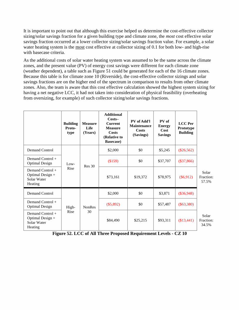
It is important to point out that although this exercise helped us determine the cost-effective collector

sizing/solar savings fraction for a given building type and climate zone, the most cost effective solar

savings fraction occurred at a lower collector sizing/solar savings fraction value. For example, a solar

water heating system is the most cost effective at collector sizing of 0.1 for both low- and high-rise

with basecase criteria.

As the additional costs of solar water heating system was assumed to be the same across the climate

zones, and the present value (PV) of energy cost savings were different for each climate zone

(weather dependent), a table such as Figure 51 could be generated for each of the 16 climate zones.

Because this table is for climate zone 10 (Riverside), the cost-effective collector sizings and solar

savings fractions are on the higher end of the spectrum in comparison to results from other climate

zones. Also, the team is aware that this cost effective calculation showed the highest system sizing for

having a net negative LCC, it had not taken into consideration of physical feasibility (overheating

from oversizing, for example) of such collector sizing/solar savings fractions.

Building

Proto-

type

Measure

Life

(Years)

Additional

Costs–

Current

Measure

Costs

(Relative to

Basecase)

PV of Add'l

Maintenance

Costs

(Savings)

PV of

Energy

Cost

Savings

LCC Per

Prototype

Building

Demand Control

Low-

Rise Res 30

$2,000 $0 $5,245 ($26,562)

Demand Control +

Optimal Design ($159) $0 $37,707 ($37,866)

Demand Control +

Optimal Design +

Solar Water

Heating

$73,161 $19,372 $78,975 ($6,912)

Solar

Fraction:

57.5%

Demand Control

High-

Rise

NonRes

30

$2,000 $0 $3,871 ($36,948)

Demand Control +

Optimal Design ($5,892) $0 $57,487 ($63,380)

Demand Control +

Optimal Design +

Solar Water

Heating

$84,490 $25,215 $93,311 ($13,441)

Solar

Fraction:

34.5%

Figure 52. LCC of All Three Proposed Requirement Levels - CZ 10

Page 76


4.3.3 Cost Effective Solar Savings Fractions

Carrying out the same LCC analysis as presented in the previous section, converting the collector

sizing to solar savings fraction and interpolating between results, we calculated the highest cost-

effective values for the rest of the climate zones displayed in Figure 53.

BASE TDV Value:

Demand Control +

Optimal design +

Cost Effective Solar Fraction

REACH TDV Value:

Demand Control +

Optimal design +

Cost Effective Solar Fraction

Climate Zone Low-Rise High-Rise Low-Rise High-Rise

1. Arcata 26% 15% 51% 47%

2. Santa Rosa 39% 22% 64% 63%

3. Oakland 47% 29% 66% 66%

4. San Jose Reid 50% 31% 69% 68%

5. Santa Maria 52% 33% 66% 66%

6. Torrance 58% 38% 76% 75%

7. San Diego 59% 39% 76% 75%

8. Fullerton 56% 37% 74% 73%

9. Burbank-Glendale 56% 36% 74% 73%

10. Riverside 62% 45% 75% 74%

11. Red Bluff 52% 35% 67% 67%

12. Sacramento 51% 34% 66% 65%

13. Fresno 49% 32% 66% 65%

14. Palmdale 67% 50% 78% 77%

15. Palm Springs 66% 46% 82% 81%

16. Blue Canyon 54% 38% 65% 64%

Figure 53. Highest Cost Effective Solar Savings Fractions

The figures displayed here are the highest solar savings fractions proven cost effective in combination

with the demand control recirculation strategy and optimal design of distribution layout. Our

calculation so far had only taken into consideration the energy savings potential and associated costs

(additional system cost and maintenance cost). In order to determine the minimum solar fraction

requirements, the following three factors are further evaluated.

Alternative compliance options

Availability of roof space

Avoidance of solar water heating system overheat

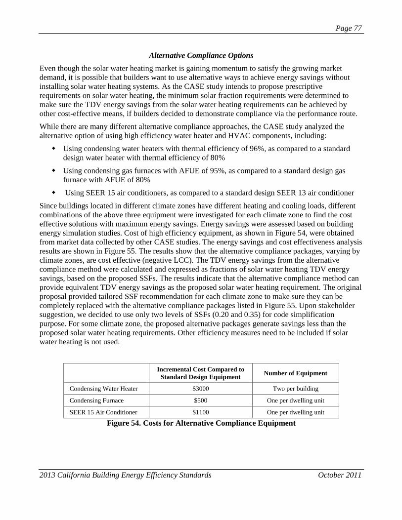
Page 77


Alternative Compliance Options

Even though the solar water heating market is gaining momentum to satisfy the growing market

demand, it is possible that builders want to use alternative ways to achieve energy savings without

installing solar water heating systems. As the CASE study intends to propose prescriptive

requirements on solar water heating, the minimum solar fraction requirements were determined to

make sure the TDV energy savings from the solar water heating requirements can be achieved by

other cost-effective means, if builders decided to demonstrate compliance via the performance route.

While there are many different alternative compliance approaches, the CASE study analyzed the

alternative option of using high efficiency water heater and HVAC components, including:

Using condensing water heaters with thermal efficiency of 96%, as compared to a standard

design water heater with thermal efficiency of 80%

Using condensing gas furnaces with AFUE of 95%, as compared to a standard design gas

furnace with AFUE of 80%

Using SEER 15 air conditioners, as compared to a standard design SEER 13 air conditioner

Since buildings located in different climate zones have different heating and cooling loads, different

combinations of the above three equipment were investigated for each climate zone to find the cost

effective solutions with maximum energy savings. Energy savings were assessed based on building

energy simulation studies. Cost of high efficiency equipment, as shown in Figure 54, were obtained

from market data collected by other CASE studies. The energy savings and cost effectiveness analysis

results are shown in Figure 55. The results show that the alternative compliance packages, varying by

climate zones, are cost effective (negative LCC). The TDV energy savings from the alternative

compliance method were calculated and expressed as fractions of solar water heating TDV energy

savings, based on the proposed SSFs. The results indicate that the alternative compliance method can

provide equivalent TDV energy savings as the proposed solar water heating requirement. The original

proposal provided tailored SSF recommendation for each climate zone to make sure they can be

completely replaced with the alternative compliance packages listed in Figure 55. Upon stakeholder

suggestion, we decided to use only two levels of SSFs (0.20 and 0.35) for code simplification

purpose. For some climate zone, the proposed alternative packages generate savings less than the

proposed solar water heating requirements. Other efficiency measures need to be included if solar

water heating is not used.

Incremental Cost Compared to

Standard Design Equipment Number of Equipment

Condensing Water Heater $3000 Two per building

Condensing Furnace $500 One per dwelling unit

SEER 15 Air Conditioner $1100 One per dwelling unit

Figure 54. Costs for Alternative Compliance Equipment

Climate

Zone

Solar Water Heating Alternative Compliance Method

Proposed

SFF

TDV

Energy

Savings-

kBtu/sqft

Efficiency Measures TDV Energy Savings PV

Energy

Savings

($/sqft)

Incremental

Cost

($/sqft)

LCC

($/sqft) HE

Water

Heater

HE

Furnace

HE

AC kBtu/sqft

Percent of Solar

Water TDV

Energy Savings

1 0.20 6.3 Yes Yes 7.5 119% $1.29 $0.73 -$0.56

2 0.20 6.1 Yes Yes 8.3 135% $1.43 $0.73 -$0.70

3 0.20 6.1 Yes Yes 6.5 107% $1.13 $0.73 -$0.40

4 0.20 6.0 Yes Yes 7.1 117% $1.23 $0.73 -$0.50

5 0.20 6.1 Yes Yes 6.7 110% $1.16 $0.73 -$0.43

6 0.20 5.9 Yes Yes 5.4 92% $0.94 $0.73 -$0.21

7 0.20 5.9 Yes Yes 5.3 90% $0.92 $0.73 -$0.18

8 0.20 5.9 Yes Yes 5.5 94% $0.96 $0.73 -$0.22

9 0.20 5.8 Yes Yes 5.5 94% $0.95 $0.73 -$0.21

10 0.35 10.2 Yes Yes 9.7 95% $1.67 $1.42 -$0.25

11 0.35 10.4 Yes Yes Yes 13.8 132% $2.39 $2.00 -$0.39

12 0.35 10.5 Yes Yes 7.6 72% $1.31 $0.73 -$0.58

13 0.35 10.2 Yes Yes Yes 13.7 135% $2.38 $2.00 -$0.38

14 0.35 10.4 Yes Yes Yes 14.6 140% $2.53 $2.00 -$0.53

15 0.35 9.4 Yes Yes Yes 18.0 191% $3.12 $2.00 -$1.12

16 0.35 11.3 Yes Yes Yes 13.9 123% $2.41 $2.00 -$0.41

Figure 55. Alternative Compliance Method to Installing Solar Water Heating

Roof Space for Solar Water Heating

There had been concerns regarding the amount of roof space needed to achieve a specified minimum

solar savings fraction requirement, especially high density multifamily buildings with smaller

footprint, therefore relatively small roof areas. Furthermore, roof space set aside for the installation of

solar thermal collectors (and photovoltaic panels) would also compete with existing mechanical

systems installed on the roof. To ensure our proposed minimum solar savings fractions were feasible

in terms of roof space constraint, the team calculated the amount of roof space needed to satisfy the

requirement and compare that to the total roof space, which is effectively the footprint of a multi-story

building.

As shown in Figure 56, with a solar savings fraction level of 50% (the highest proposed level is 35%

for climate zones 10-15), the corresponding collector sizing ratio is approximately 0.4 ft2 per gal/day

hot water demand. The resulting collector area needed for the low-rise and high-rise building

prototypes respectively accounts for 3% and 6% of the building footprints, which are roughly the

amount of roof space theoretically available. Furthermore, with fixed daily hot water demand

numbers, we calculated the collector area in percentage building footprint for buildings with different

number of stories. With a 20-story multifamily building with the same daily hot water demand (the

same number of units with the same CFA each), the collector area necessary to achieve a solar

savings fraction of 50% would only account for 28% of the total available roof space (Figure 57).

Building Prototype Unit low-rise high-rise

Daily hot water demand gal/day 1,347

Building footprint ft2 19,140 19,140

Number of stories 2 4

Solar savings fraction 50% 50%

corresponding collector sizing ratio ft2/ gal/day 0.4 0.4

Resulting collector area ft2 539 1,159

% of building footprint % total 3% 6%

Figure 56. Collector Area in % Total of Building Footprint Calculation (SSF = 50%)

Number of Stories % of building footprint

2 3%

3 4%

4 6%

5 7%

10 14%

20 28%

Figure 57. Roof Area for Solar Collectors (SSF = 50%)

Page 80


Overheating Issue due to Oversizing

Industry stakeholders reflected that while the issue of freeze protection has been widely explored (the

development of various solar water heating system types is a reflection of this evolution), the issue of

overheating is often not considered as seriously as it should be, especially for climate conditions with

relatively high solar insolation level such as California. When a solar water heating system is

designed with a relatively high annual solar savings fraction, the monthly solar fractions during the

summer months are maxed out to 100%, and the unintended consequence of overheating occurs. To

be conservative, stakeholders have suggested for the team to cap out the solar savings fraction

requirement at 50%. This suggestion was followed as the highest solar fraction requirement the team

is proposing (for CZ 15) is 35%.

4.3.4 Solar Water Heating Ready Measure Cost Effective Adoption Rates

Costs, potential cost savings and estimated minimum cost effective adoption rates for solar water

heating ready buildings are displayed in Figure 58. Although the construction start estimates for low

and high-rise multifamily buildings in 2013 are included in this calculation, these numbers do not

change the resulting adoption rates, as the adoption rates are mathematically the ratio between these

two terms described in Section 3.2.5:

)(__ newinstalltotalready MFMFCostNowCostAdditional

)(__ retrofityearsnretrofit MFFVMCostLaterSavingsCost

Calculations show that in order for the solar water heating ready measure to be cost effective, at least

half of the buildings would have to retrofit for solar water heating systems during the 30 years

measure life length (from 2013-2043), assuming a 15% cost savings and a linear adoption curve.

Building Prototype Low-rise Hig hrise

# new buildings in 2013 272 202

Installation at new const 1% 1%

Remaining bldg w/t installation at new const 269 200

per bldg "ready" cost $2,782 $6,047

Ready Costs associated $749,562 $ 1,208,671

Minimum Cost Effective Adoption Rate

with 10% cost savings 73% 75%

with 15% cost savings 49% 50%

Figure 58. Cost Effective Adoption Rates for Ready Measure

We explored a few sources of future market penetration for solar water heating systems to determine

the likelihood of such adoption rates. We reviewed the same literature and followed a similar logic as

the Solar Ready Homes and Solar Oriented Development CASE topic (for single family homes),

There are three major sources of future market penetration rates:

California Statewide Residential Appliance Saturation Study (RASS) 2009

Page 81


California Statewide Residential Sector Energy Efficiency Potential Study

CSI-Thermal program energy savings goals

CPUC’s California Long Term Energy Efficiency Strategic Plan

The 2009 RASS database provided a current market penetration of ~ 1% (Figure 33), and the Energy

Efficiency Potential Study established the upper bound of penetration rate (close to 100%).

Unfortunately, it is challenging to extract the number of multifamily building solar water heating

installations expected from the CSI-thermal program energy savings goals2, due to the difficulty in

defining an average sized building and system and that the goal is a combined goal for single-family,

multifamily and commercial buildings within the state.

The last identified source of future market penetration rate, California’s Long Term EE Strategic Plan,

calls for

All new residential construction in California be zero net energy by 2020,

25% of existing homes will achieve 70% decrease in purchased energy, relative to 2008 levels

75% of existing homes will achieve 30% decrease in purchased energy, relative to 2008 levels

To accomplish the goal of being zero net energy, it is reasonable to expect that t solar water heating

systems will be installed in all new constructions. For the 25% of existing buildings that would need

to achieve 70% reduction in purchase energy, the installation of renewable technology is inevitable.

Therefore, if this level of solar water heating penetration is needed to achieve the state’s grand vision

of energy efficiency, an equivalent housing stock (both new construction and existing buildings)

adoption rate would be higher than 25% by 2020.

Furthermore, our calculation assumed that the solar tank space reservation is inside, rather than

outside the building. If the space reserved for future solar equipment (tank) is outside, the ready

measure would imply merely installing a concrete pad at the time of new construction. The

calculation of the minimum cost effective adoption rates for solar water heating ready measure did not

factor in the probable reduction in installed system pricing due to various program efforts. Another

conservative assumption built into the calculation is the exclusion of any energy savings benefits as

the results of the installation of solar water heating system, promoted by the ready measures.

Accounting for the above-mentioned references and reasons, the team concluded the proposed solar

water heating ready measure cost effective. The space reserved for potential solar collectors shall be

roof space equivalent to solar savings fraction of 50%, marginally exceeding the highest solar savings

fractions requirement (45%) across climate zones. This calculation of the reserved space needed will

be a function of the number of the story of the building to account for decreasing building footprint

with increasing number of story.

2 Program goal includes “achieving the installation of natural gas-displaying systems that displace 585 million therms over the 25-year life of the

systems.”

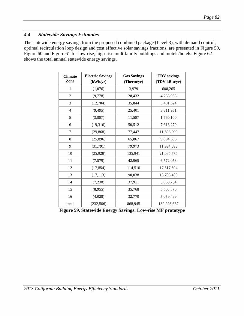
Page 82


4.4 Statewide Savings Estimates

The statewide energy savings from the proposed combined package (Level 3), with demand control,

optimal recirculation loop design and cost effective solar savings fractions, are presented in Figure 59,

Figure 60 and Figure 61 for low-rise, high-rise multifamily buildings and motels/hotels. Figure 62

shows the total annual statewide energy savings.

Climate

Zone

Electric Savings

(kWh/yr)

Gas Savings

(Therm/yr)

TDV savings

(TDV kBtu/yr)

1 (1,076) 3,979 608,265

2 (9,778) 28,432 4,263,968

3 (12,704) 35,844 5,401,624

4 (9,495) 25,401 3,811,951

5 (3,887) 11,587 1,760,100

6 (19,316) 50,512 7,616,270

7 (29,868) 77,447 11,693,099

8 (25,896) 65,867 9,894,636

9 (31,791) 79,973 11,994,593

10 (25,928) 135,941 21,035,775

11 (7,579) 42,965 6,572,053

12 (17,854) 114,510 17,517,304

13 (17,113) 90,038 13,705,405

14 (7,238) 37,911 5,860,754

15 (8,955) 35,768 5,503,370

16 (4,028) 32,770 5,059,499

total (232,506) 868,945 132,298,667

Figure 59. Statewide Energy Savings: Low-rise MF prototype

Page 83


Climate

Zone

Electric Savings

(kWh/yr)

Gas Savings

(Therm/yr)

TDV savings

(TDV kBtu/yr)

1 - - -

2 (2,006) 5,782 884,497

3 (21,127) 58,094 8,938,415

4 (25,124) 64,738 9,910,210

5 (2,316) 6,816 1,057,705

6 (25,449) 63,417 9,772,452

7 (16,691) 41,166 6,352,857

8 (37,268) 89,777 13,769,339

9 (44,001) 104,574 16,008,448

10 (9,306) 54,835 8,626,114

11 (678) 4,415 687,376

12 (12,146) 93,750 14,594,648

13 (2,156) 12,710 1,968,220

14 - - -

15 - - -

16 - - -

total (198,268) 600,074 92,570,282

Figure 60. Statewide Energy Savings: High-rise MF prototype

Page 84


Climate

Zone

Electric Savings

(kWh/yr)

Gas Savings

(Therm/yr)

TDV savings

(TDV kBtu/yr)

1 (491) 1,859 287,304

2 (5,288) 15,317 2,317,729

3 (14,986) 41,793 6,357,494

4 (15,331) 40,320 6,105,366

5 (2,771) 8,214 1,259,852

6 (10,005) 25,597 3,897,493

7 (13,619) 34,520 5,263,535

8 (19,488) 48,359 7,332,795

9 (45,624) 111,846 16,930,053

10 (3,987) 22,021 3,433,582

11 (1,869) 11,268 1,737,749

12 (13,219) 91,946 14,179,873

13 (5,930) 32,821 5,035,742

14 (2,330) 12,853 2,001,586

15 (660) 2,689 417,138

16 (1,581) 14,510 2,258,644

total (157,179) 515,934 78,815,933

Figure 61. Statewide Energy Savings: Motels/Hotels

Building Type Electric Savings

(GWh/yr)

Gas Savings

(MMT/yr)

TDV savings (TDV

MBtu/yr)

Low-Rise MF (0.23) 0.87 132,299

High-Rise MF (0.20) 0.60 92,570

Hotel/Motel (0.16) 0.52 78,816

Total (0.59) 1.98 303,685

Figure 62. Total Statewide Energy Savings

Page 85


5. Recommended Language for the Standards Document,

ACM Manuals, and the Reference Appendices

The recommended code language below incorporates inputs from various stakeholders and CEC staff,

received throughout the IOUs stakeholder meetings and CEC’s pre-rulemaking processes. For a

complete evolution of changes in recommended language, please refer to Appendix 7.7.

The original proposal recommended different levels of solar savings fractions (SSF) according to

measure cost-effective characteristics in each climate. During the pre-rulemaking workshop, industry

stakeholders suggested that the number to SSFs be reduced for easy implementation. Upon discussion

with CEC staff, we recommend that only two levels of SSFs be used, 0.2 (for CZ1-9) and 0.35 (CZ10-

16). This simplification is based on the originally proposed SSF. The proposed SSFs are slightly

increased for some climates and reduced for others. The averaged SSF overall all 16 climate zones

stay the same at 0.27.

5.1 Section 101(b)

DEMAND CONTROL (for central water heating) is an automatic control system that controls the

recirculation pump operation based on measurement of hot water demand and hot water return

temperature.

SOLAR SAVINGS FRACTION (SSF) is the fraction of domestic hot water demand provided by

solar hot water heating, according to Residential ACM Appendix E equation RE-1. The value of SSF

shall be determined using the approved solar water heating calculations methods based on results

from the OC-100 and OG-300 test procedure.

TEMPERATURE MODEULATION CONTROL (for central water heating) is an automatic control

system that reduced hot water supply temperature when hot water demand is expected to be low.

5.2 Section 151(f) 8C

C. For systems serving multiple dwelling units, with a central water heating system that

includes the following components shall be installed:

1. gGas or propane water heaters, boilers or other water heating equipment that

meet the minimum efficiency requirements of Sections 111 and 113., and

2. A water heating recirculation loop system that meets the requirements of

Section 113(c)2 and Section 113(c)5 and is equipped with a demand control

and has two recirculation loops each serving half of the building, and

EXCEPTION 1 to Section 151(f)8c 2: Buildings with eight or few units are

exempt from the requirements on having two recirculation loops.

3. A solar water heating system with a minimum solar savings fraction of 0.20 for

climate zones 1 through 9 and 0.35 climate zones 10 through 16.

5.3 Section 113(c)2

2. Controls for hot water distribution systems. Service hot water systems with

circulating pumps or with electrical heat trace systems shall be capable of

automatically turning off the system.

EXCEPTION 1 to Section 113(c)2: Water heating systems serving a single dwelling

unit.

EXCEPTION 2 to Section 113(c)2: Recirculation systems serving multiple dwelling

units and equipped with temperature modulation control.

5.4 Section 150(n)

(n) Water Heating Recirculation Loops Serving Multiple Dwelling Units. Water heating recirculation

loops serving multiple dwelling units shall meet the requirements of Section 113(c)5.

(n) Water Heating System Serving Multiple Dwelling Units.

1. Water heating recirculation loops serving multiple dwelling units shall meet the

requirements of Section 113(c)5.

2. The following items shall be clearly shown and labeled on building plans/drawings

submitted for building permit:

A. Marked solar zone on the roof and/or structures attached to the building:

1. The solar zone shall be at least 1.5 % of building conditioned floor area

or 30% of the total available roof area whichever is smaller and be

oriented between 90° and 270°.

- Exception 1 to Section 150(n)2A1: The area of roof shaded

from existing trees, utility poles, other buildings, and other non-

building sources are exempted from the available roof area

requirement.

2. The solar zone shall be minimally shaded by vents, chimneys,

architectural features, mechanical equipment or other obstructions that

are on the roof or any other part of the building. Any vent, chimney, or

other architectural feature shall be a minimum distance of twice the

height from the solar zone(s).

- Exception 1 to Section 150(n)2A2: Any vent, chimney, or

other architectural feature to the north of the solar zone(s) shall

be exempt from the minimum shading requirement.

3. The solar zone may be comprised of smaller sub-areas. No sub-area

shall be smaller than 33% of the total solar zone or smaller than 80 sqft.

All sub-areas must be at least 5 feet wide in the narrowest dimension.

4. The solar zone shall be sited in compliance with Section 2 of the

California Department of Forestry and Fire Protection Office of the

State Fire Marshal Solar Photovoltaic Installation Guideline.

Page 87


B. Marked solar tank area with a minimum area in sqft determined by:

0.0004 x building CFA + 13.

The area must be at least 4 feet wide in the narrowest dimension.

C. Marked plumbing and conduit paths between the solar zone and the solar tank

area.

D. Marked plumbing and conduit paths between the solar tank area and the water

heater(s)/boiler(s).

EXCEPTION 1 to Section 150(n)2: Buildings with an installed solar water heating system that meets

Section 151(f) 8C iii.

5.5 Reference Appendix 9.1.1

For the Joint Appendix, the team recommends the following organization and language:

9 Solar Energy Systems

9.1 Solar Thermal Systems

9.1.1 Solar Water Heating Systems

Solar water heating systems for individual dwellings shall be rated with the OG 300 procedures. shall

satisfy the following eligibility criteria:

In order to use the OG-300 method, the system must satisfy the following eligibility criteria:

1. The system shall be SRCC certified using the OG-100 or OG-300 procedures. Systems used

for individual residential dwellings shall be certified using the OG-300 procedure.

2. The collectors must shall face within 35 degrees of south and be tilted at a slope of at least

3:12

The system shall be SRCC certified.

3. The system must Systems using OG-300 certification shall be installed in the exact

configuration for which it was rated, e.g. the system must have the same collectors, pumps,

controls, storage tank and backup water heater fuel type as the rated condition.

4. The system must shall be installed according to manufacturer’s instructions.

5. The collectors shall be located in a position that is not shaded by adjacent buildings or trees

between 9:00 AM and 3:00 PM (solar time) on December 21.

9.1.2 Solar Space Heating Systems

9.2 Photovoltaic Systems

Page 88


6. Bibliography and Other Research

RSMeans Costworks Online Construction Cost Data, 2010 Residential Cost Books. Online edition.

http://www.meanscostworks.com/

Energy Information Administration, Solar Thermal Collector Manufacturing Activities 2009,

http://www.eia.doe.gov/cneaf/solar.renewables/page/solarreport/solar.html

KEMA-XENERGY, California Statewide Residential Appliance Saturation Study. Online Database,

2009, http://websafe.kemainc.com/RASS2009/Default.aspx

Itron, prepared for California Center for Sustainable Energy, Solar Water Heating Pilot Program:

Interim Evaluation Report, Jan 2009

California Solar Initiative- Thermal, Website. http://www.gosolarcalifornia.org/solarwater/

Intelligent Energy, Europe, Solar Thermal Ordinance, http://www.solarordinances.eu/

Natural Resources Canada , Solar Ready Guidelines draft, 2010,

http://oee.nrcan.gc.ca/residential/new-houses.cfm

Build It Green, GreenPoint Rated Single Family New Construction, 2009-11 version.

US Green Building Council, LEED 2009 for New and Major Renovations.

American Society of Heating, Refrigerating and Air-Conditioning Engineers, Proposed Updates to

ASHRAE 189.1 Renewable Sections, 2010.

Lisell L., Tetreault T., and Watson A., NREL, Solar Ready Building Planning Guide, Dec 2009.

California Department of Forestry and Fire Protection, Office of the State Fire Marshal, Solar

Photovoltaic Installation Guideline, Apr 2008,

http://osfm.fire.ca.gov/pdf/reports/solarphotovoltaicguideline.pdf.

Codes and Standards Enhancement Initiative Team, Space and Water Heating ACM Improvement

Draft Report, May 2011.

Codes and Standards Enhancement Initiative Team, Solar Ready Homes and Solar Oriented

Developments Draft Report, May 2011.

http://www.meanscostworks.com/

http://www.eia.doe.gov/cneaf/solar.renewables/page/solarreport/solar.html

http://websafe.kemainc.com/RASS2009/Default.aspx

http://www.gosolarcalifornia.org/solarwater/

http://www.solarordinances.eu/

http://oee.nrcan.gc.ca/residential/new-houses.cfm

http://osfm.fire.ca.gov/pdf/reports/solarphotovoltaicguideline.pdf

Page 89


7. Appendices

7.1 Recirculation Loop Model Validation Results

Building 1. Recirculation loop loss represent 34% Total hot water energy


SFDMeasured

(Btu/day)

Modeled

(Btu/day)

Measured

reduction

(%)

Modeled

reduction

(%)

Measured

(Btu/day)

Modeled

(Btu/day)

Measured

reduction

(%)

Modeled

reduction

(%)

Measured

(Btu/day)

Modeled

(Btu/day)

Measured

reduction

(%)

Modeled

reduction

(%)

CONT Pump 608,711 608,711 - - 639,732 643,487 - - 1,875,663 1,879,417 - -

Temp Mod 600,697 582,695 1.3% 4.3% 633,433 616,266 1.0% 4.2% 1,958,764 1,941,597 -4.4% -3.3%

Timer 507,048 461,656 17% 24% 600,803 562,822 6.1% 13% 1,732,428 1,694,446 7.6% 10%

Demand 215,483 191,328 65% 69% 411,903 453,556 36% 30% 1,423,628 1,465,281 24% 22%

Total Hot Water EnergyRecirculation Flow Heat Loss Recirculation Loop Heat Loss

SAMMeasured

(Btu/day)

Modeled

(Btu/day)

Measured

reduction

(%)

Modeled

reduction

(%)

Measured

(Btu/day)

Modeled

(Btu/day)

Measured

reduction

(%)

Modeled

reduction

(%)

Measured

(Btu/day)

Modeled

(Btu/day)

Measured

reduction

(%)

Modeled

reduction

(%)

CONT Pump 368,536 368,536 - - 443,280 456,190 - - 1,030,479 1,043,388 - -

Temp Mod 362,987 355,698 1.5% 3.5% 442,840 435,949 0.1% 4.4% 1,030,039 1,023,148 0.0% 1.9%

Timer 265,214 279,559 28% 24% 421,494 419,521 5% 8% 1,008,693 1,006,720 2.1% 3.5%

Demand


Page 90



Comparison to measured results


Comparison to measured results

SFFMeasured

(Btu/day)

Modeled

(Btu/day)

Measured

reduction

(%)

Modeled

reduction

(%)

Measured

(Btu/day)

Modeled

(Btu/day)

Measured

reduction

(%)

Modeled

reduction

(%)

Measured

(Btu/day)

Modeled

(Btu/day)

Measured

reduction

(%)

Modeled

reduction

(%)

CONT Pump 176,588 176,588 - - 221,165 228,267 - - 3,116,211 3,123,313 - -

Temp Mod 157,692 159,541 11% 10% 204,820 204,057 7% 11% 2,564,910 2,564,146 18% 18%

Timer 151,829 147,709 14% 16% 220,452 228,777 0.3% -0.2% 3,443,807 3,452,131 -11% -11%

Demand 48,168 78,002 73% 56% 178,093 179,729 19% 21% 2,784,551 2,786,187 11% 11%


SFHMeasured

(Btu/day)

Modeled

(Btu/day)

Measured

reduction

(%)

Modeled

reduction

(%)

Measured

(Btu/day)

Modeled

(Btu/day)

Measured

reduction

(%)

Modeled

reduction

(%)

Measured

(Btu/day)

Modeled

(Btu/day)

Measured

reduction

(%)

Modeled

reduction

(%)

CONT Pump 177,796 177,796 - - 201,589 207,200 - - 1,094,813 1,100,423 - -

Temp Mod - - - - - - - -

Timer 143,549 145,345 19% 18% 187,240 194,233 7% 6% 942,592 949,586 14% 14%

Demand 90,349 82,244 49% 54% 180,478 173,723 10% 16% 742,710 735,955 32% 33%


7.2 Screenshots of the Recirculation Model

Page 92


7.3 Solar Water Heating Online Survey Instrument

7.4 Example of Solar Water Heating Ready Ordinances

7.5 Energy Saving: Solar Water Heating Simulation Results

7.5.1 Comparison between Climate Zones (high-rise prototype)

40%

50%

60%

70%

80%

90%

100%

1 2 3 4 5 6 7 8 9 10 11 12 13 14 15 16

An

nu

al S

ola

r Fr

atio

n

California Climate Zones

Solar Fraction: High Rise Prototype

Active Glycol (External HX) Active Glycol (immersed HX) Water Drainback Forced Circulation

Page 94

2013 California Building Energy Efficiency Standards June 2011

7.5.2 Comparison between Various Configurations

Low-rise Prototype

Active Glycol (External HX)

Climate Zone

City

Electricity

Use

Natural

Gas

Savings

TDV

Electricity

Savings

TDV Gas

Savings

PV of

Energy

Cost

Savings

Solar

Savings

Fraction

(kwh/yr) (Therms/yr) (TDV

kBTU)

(TDV

kBTU) (PV$) (%)

1. Arcata 2,194 2,660 (54,648) 409,985 61,540 59%

2. Santa Rosa 2,145 3,167 (47,481) 488,551 76,388 73%

3. Oakland 2,223 3,175 (50,665) 490,789 76,224 73%

4. San Jose Reid 2,162 3,232 (47,029) 501,627 78,731 76%

5. Santa Maria 2,274 3,479 (51,366) 546,500 85,751 81%

6. Torrance 2,320 3,330 (51,665) 524,495 81,888 81%

7. San Diego 2,280 3,366 (50,857) 533,019 83,505 83%

8. Fullerton 2,181 3,274 (47,130) 515,347 81,090 81%


10. Riverside 2,126 3,269 (45,102) 515,756 81,512 82%

11. Red Bluff 2,018 3,043 (42,816) 470,790 74,120 74%

12. Sacramento 2,092 3,038 (44,886) 466,491 73,017 72%

13. Fresno 1,921 2,863 (40,138) 440,304 69,304 72%

14. Palmdale 2,174 3,487 (45,305) 550,798 87,545 85%

15. Palm Springs 2,016 3,076 (40,952) 488,795 77,561 90%

16. Blue Canyon 2,201 3,338 (47,464) 518,440 81,567 71%

Page 95


Active Glycol (Immersed HX)

Climate Zone

City

Electricity

Use

Natural Gas

Savings

TDV

Electricity

Savings

TDV Gas

Savings

PV of

Energy

Cost

Savings

Solar

Savings

Fraction


kBTU)

(TDV

kBTU) (PV$) (%)

1. Arcata 6,345 2,587 (140,325) 397,837 44,598 57%

2. Santa Rosa 6,224 3,163 (134,268) 486,176 60,946 73%

3. Oakland 6,300 3,158 (136,753) 486,355 60,547 73%

4. San Jose Reid 6,227 3,230 (133,698) 499,297 63,317 76%

5. Santa Maria 6,332 3,465 (137,255) 542,275 70,145 80%

6. Torrance 6,370 3,310 (137,834) 519,421 66,086 81%

7. San Diego 6,348 3,359 (137,286) 530,030 68,019 83%

8. Fullerton 6,261 3,275 (134,158) 513,498 65,697 81%


10. Riverside 6,187 3,267 (132,015) 513,636 66,092 82%

11. Red Bluff 6,111 3,045 (130,425) 469,119 58,658 74%

12. Sacramento 6,162 3,043 (131,944) 465,561 57,779 72%

13. Fresno 6,050 2,866 (128,688) 439,257 53,787 72%

14. Palmdale 6,176 3,485 (131,308) 548,183 72,198 85%

15. Palm Springs 6,026 3,070 (127,926) 486,493 62,099 89%

16. Blue Canyon 6,235 3,327 (133,829) 514,503 65,928 71%

Page 96


Forced Circulation

Climate Zone /

City

Electricity

Use

Natural

Gas

Savings

TDV

Electricity

Savings

TDV Gas

Savings

PV of

Energy

Cost

Savings

Solar

Savings

Fraction


kBTU)

(TDV

kBTU) (PV$) (%)

1. Arcata 5,444 2,783 (117,683) 429,637 54,027 61%

2. Santa Rosa 5,534 3,233 (118,204) 499,482 66,033 75%

3. Oakland 5,528 3,265 (118,292) 506,108 67,165 76%

4. San Jose Reid 5,534 3,285 (117,980) 510,289 67,943 77%

5. Santa Maria 5,602 3,561 (119,886) 560,789 76,359 83%

6. Torrance 5,553 3,428 (118,638) 541,186 73,180 83%

7. San Diego 5,561 3,462 (118,710) 549,427 74,595 86%

8. Fullerton 5,546 3,365 (118,153) 530,974 71,496 84%


10. Riverside 5,551 3,352 (117,957) 530,087 71,376 84%

11. Red Bluff 5,495 3,111 (116,794) 482,286 63,299 75%

12. Sacramento 5,485 3,104 (116,761) 477,564 62,487 74%

13. Fresno 5,465 2,925 (115,995) 450,957 58,011 74%

14. Palmdale 5,574 3,510 (118,091) 554,433 75,569 85%

15. Palm Springs 5,497 3,136 (116,281) 499,486 66,366 91%

16. Blue Canyon 5,660 3,308 (120,082) 512,623 67,983 70%

Page 97


Evacuated Tube (External HX)

Climate Zone

City

Electricity

Use

Natural Gas

Savings

TDV

Electricity

Savings

TDV Gas

Savings

PV of

Energy

Cost

Savings

Solar

Savings

Fraction


kBTU)

(TDV

kBTU) (PV$) (%)

1. Arcata 4,477 5,486 (113,352) 847,381 127,125 61%

2. Santa Rosa 4,362 6,417 (99,172) 991,663 154,569 75%

3. Oakland 4,500 6,418 (105,070) 993,579 153,879 75%

4. San Jose Reid 4,368 6,523 (97,482) 1,013,541 158,651 78%

5. Santa Maria 4,631 6,997 (107,506) 1,099,606 171,820 82%

6. Torrance 4,702 6,703 (107,918) 1,055,982 164,193 83%

7. San Diego 4,627 6,802 (106,348) 1,077,026 168,110 85%

8. Fullerton 4,426 6,598 (98,065) 1,038,470 162,867 83%

9. Burbank-Glendale 4,364 6,559 (94,674) 1,033,575 162,606 84%

10. Riverside 4,304 6,588 (93,571) 1,039,973 163,906 84%

11. Red Bluff 4,104 6,182 (88,983) 958,384 150,570 76%

12. Sacramento 4,244 6,177 (93,359) 950,982 148,530 74%

13. Fresno 3,929 5,851 (83,796) 902,936 141,865 75%

14. Palmdale 4,380 7,024 (93,100) 1,110,821 176,257 87%

15. Palm Springs 3,994 6,198 (82,581) 986,351 156,522 92%

16. Blue Canyon 4,488 6,815 (99,750) 1,059,949 166,295 73%

Page 98


High-rise Prototype

Active Glycol (External HX)

Climate Zone

City

Electricity

Use

Natural

Gas

Savings

TDV

Electricity

Savings

TDV Gas

Savings

PV of

Energy

Cost

Savings

Solar

Savings

Fraction


kBTU)

(TDV

kBTU) (PV$) (%)

1. Arcata 4,411 5,254 (110,212) 809,132 121,045 58%

2. Santa Rosa 4,314 6,294 (95,933) 970,135 151,401 73%

3. Oakland 4,477 6,307 (102,462) 974,233 150,980 73%

4. San Jose Reid 4,348 6,427 (94,942) 996,699 156,174 76%

5. Santa Maria 4,579 6,916 (103,843) 1,085,785 170,061 80%

6. Torrance 4,671 6,619 (104,400) 1,041,922 162,368 81%

7. San Diego 4,591 6,698 (102,863) 1,060,034 165,771 83%

8. Fullerton 4,386 6,511 (95,057) 1,024,264 160,928 81%


10. Riverside 4,278 6,502 (91,017) 1,025,348 161,815 82%

11. Red Bluff 4,061 6,050 (86,492) 935,186 146,984 73%

12. Sacramento 4,198 6,037 (90,464) 926,162 144,733 72%

13. Fresno 3,863 5,690 (81,012) 874,316 137,391 72%

14. Palmdale 4,383 6,940 (91,549) 1,095,555 173,882 84%

15. Palm Springs 4,055 6,130 (82,582) 973,543 154,304 89%

16. Blue Canyon 4,424 6,628 (95,816) 1,028,517 161,533 70%

Page 99


Active Glycol (Immersed HX)

Climate Zone

City

Electricity

Use

Natural

Gas

Savings

TDV

Electricity

Savings

TDV Gas

Savings

PV of

Energy

Cost

Savings

Solar

Savings

Fraction


kBTU)

(TDV

kBTU) (PV$) (%)

1. Arcata 12,737 5,112 (281,822) 785,536 87,237 56%

2. Santa Rosa 12,494 6,290 (270,069) 966,033 120,533 73%

3. Oakland 12,648 6,275 (274,939) 965,733 119,637 73%

4. San Jose Reid 12,498 6,427 (268,783) 992,699 125,374 76%

5. Santa Maria 12,716 6,891 (276,009) 1,077,945 138,886 80%

6. Torrance 12,790 6,581 (277,193) 1,031,955 130,716 80%

7. San Diego 12,747 6,684 (276,257) 1,054,241 134,738 83%

8. Fullerton 12,566 6,517 (269,645) 1,021,330 130,183 81%


10. Riverside 12,413 6,502 (265,227) 1,021,556 130,987 82%

11. Red Bluff 12,255 6,054 (261,881) 932,069 116,069 73%

12. Sacramento 12,359 6,052 (265,081) 924,911 114,275 72%

13. Fresno 12,130 5,698 (258,371) 872,442 106,350 72%

14. Palmdale 12,387 6,936 (263,641) 1,090,426 143,189 84%

15. Palm Springs 12,081 6,116 (256,874) 968,577 123,258 89%

16. Blue Canyon 12,509 6,613 (268,954) 1,021,737 130,373 70%

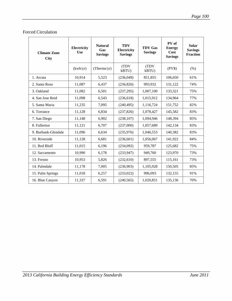
Page 100


Forced Circulation

Climate Zone

City

Electricity

Use

Natural

Gas

Savings

TDV

Electricity

Savings

TDV Gas

Savings

PV of

Energy

Cost

Savings

Solar

Savings

Fraction


kBTU)

(TDV

kBTU) (PV$) (%)

1. Arcata 10,914 5,523 (236,049) 851,855 106,650 61%

2. Santa Rosa 11,087 6,437 (236,826) 993,932 131,122 74%

3. Oakland 11,082 6,501 (237,295) 1,007,100 133,321 75%

4. San Jose Reid 11,098 6,543 (236,618) 1,015,912 134,964 77%

5. Santa Maria 11,235 7,095 (240,495) 1,116,724 151,752 82%

6. Torrance 11,128 6,834 (237,826) 1,078,427 145,582 83%

7. San Diego 11,148 6,902 (238,107) 1,094,946 148,394 85%

8. Fullerton 11,121 6,707 (237,000) 1,057,689 142,134 83%


10. Riverside 11,128 6,681 (236,601) 1,056,067 141,922 84%

11. Red Bluff 11,015 6,196 (234,092) 959,787 125,682 75%

12. Sacramento 10,990 6,178 (233,947) 949,760 123,970 73%

13. Fresno 10,953 5,826 (232,610) 897,555 115,161 73%

14. Palmdale 11,178 7,005 (236,903) 1,105,928 150,505 85%

15. Palm Springs 11,018 6,257 (233,022) 996,093 132,155 91%

16. Blue Canyon 11,337 6,591 (240,565) 1,020,851 135,136 70%

Page 101


Water Drainback

Climate Zone

City

Electricity

Use

Natural

Gas

Savings

TDV

Electricity

Savings

TDV Gas

Savings

PV of

Energy

Cost

Savings

Solar

Savings

Fraction


kBTU)

(TDV

kBTU) (PV$) (%)

1. Arcata 10,966 5,590 (237,654) 862,456 108,208 62%

2. Santa Rosa 11,157 6,543 (238,680) 1,010,873 133,735 76%

3. Oakland 11,150 6,566 (238,958) 1,016,552 134,670 76%

4. San Jose Reid 11,176 6,675 (238,606) 1,037,893 138,427 79%

5. Santa Maria 11,299 7,187 (242,229) 1,131,060 153,935 83%

6. Torrance 11,218 6,898 (239,764) 1,087,995 146,904 84%

7. San Diego 11,229 6,968 (239,875) 1,104,851 149,804 86%

8. Fullerton 11,191 6,768 (238,709) 1,066,766 143,410 84%


10. Riverside 11,188 6,741 (237,950) 1,065,284 143,284 85%

11. Red Bluff 11,087 6,275 (235,840) 972,411 127,565 76%

12. Sacramento 11,066 6,254 (235,864) 961,826 125,728 74%

13. Fresno 11,023 5,900 (234,152) 908,924 116,862 74%

14. Palmdale 11,249 7,182 (238,532) 1,136,413 155,502 87%

15. Palm Springs 11,090 6,295 (234,516) 1,001,875 132,897 92%

16. Blue Canyon 11,166 6,922 (238,054) 1,076,977 145,292 73%

Page 102


7.6 System Assumptions from CSI-Thermal Incentive Calculator Documentation

7.7 Evolution of Recommended Code Language

This section documents the versions of proposed language produced by the CASE team for the

combined Multi-Family Domestic Hot Water and Solar Water Heating topic. Changes occurred

between the versions are shown in red to help accentuate the differences. The evolution of the

versions is summarized below:

1. First version: HMG’s version presented in the CEC pre-rulemaking workshop on 6/9/2011

2. Second version: Revised HMG version based on comments collected during the CEC pre-

rulemaking workshop

3. CalSEIA’s recommendation

4. Third version: Revised HMG version based on consideration of CalSEIA input.

7.7.1 First Version

Section 151(f) 8C

C. For systems serving multiple dwelling units, a central water heating system that

includes the following components shall be installed: that has



2. A solar water heating system with solar fraction specified in Table 151-C, and

3. and aA water heating recirculation loop system that meets the requirements of


and has two recirculation loops each serving half of the building. shall be

installed.

Table 151-C

Climate Zone

1 2 3 4 5 6 7 8 9 10 11 12 13 14 15 16

Page 103


(requirements for other building components and systems – no change)

WATER-

HEATING

General System shall meet Section 151(f)8 or Section 151(b)1

Solar Savings

Fraction for

multifamily

buildings

0.2 0.25 0.2 0.2 0.2 0.15 0.15 0.15 0.15 0.3 0.40 0.25 0.35 0.45 0.50 0.4

Section 113(c)2




EXCEPTION to Section 113(c)2: Water heating systems serving a single dwelling

unit.

Section 150(n)








A. Marked solar zone for potential future solar collectors on the roof or other

available space on the building site







requirement.





height from the reserved area(s).


other architectural feature to the north of the reserved roof area(s)

shall be exempt from the minimum shading requirement.

Page 104




State Fire Marshal Solar Photovoltaic Installation Guideline

B. Marked solar tank area for potential solar water heating storage tank

installation of a minimum X sf or X% of conditioned floor area


area


heater(s)/boiler(s)

EXCEPTION to Section 150(n)2: Buildings with an installed solar water heating system that meets

Section 151(f) 8C ii.

7.7.2 Second Version

Section 151(f) 8C

D. For systems serving multiple dwelling units, a central water heating system that




2. A solar water heating system with solar savings fraction specified in Table 151-

C, and

3. and aA water heating recirculation loop system that meets the requirements of


and has two recirculation loops each serving half of the building. shall be

installed

Table 151-C

Climate Zone

1 2 3 4 5 6 7 8 9 10 11 12 13 14 15 16


WATER-

HEATING


Solar Savings

Fraction for

multifamily

buildings

0.2 0.25 0.2 0.2 0.2 0.15 0.15 0.15 0.15 0.3 0.40 0.25 0.35 0.45 0.45 0.4

Section 113(c)2

Page 105





EXCEPTION to Section 113(c)2: Water heating systems serving a single

dwelling unit.

Section 150(n)















requirement.





height from the reserved area(s).


other architectural feature to the north of the reserved roof

area(s) shall be exempt from the minimum shading requirement.


shall be smaller than 80 sqft, and all areas must be at least 5 feet wide in

the narrowest dimension.



State Fire Marshal Solar Photovoltaic Installation Guideline

B. Marked solar tank area with a minimum area in sqft determined by:

0.0004 x building CFA + 13

The area must be at least 4 ft wide in the narrowest dimension.

Page 106



area


heater(s)/boiler(s)

EXCEPTION to Section 150(n)2: Buildings with an installed solar water heating system that meets

Section 151(f) 8C ii are exempt from the solar water heating ready requirements.

7.7.3 CalSEIA’s Written Comment

Section 150(n)






shall be smaller than 33 percent of the total area of the solar zone, and

all areas must be at least 18 feet wide in the east-west dimension, and

15 feet wide in the north-south dimension.

B. Marked solar storage tank area (marked area) with a minimum area in square

feet equivalent to no less than 1.6 square feet of flat, structurally adequate area

for each 10 square feet of solar collector area. The marked area must be at least

10 feet wide in the narrowest dimension

1. The marked area may be inside or outside the structure upon which the

solar collectors are mounted.

2. There must be sufficient access to accommodate the movement of a

solar storage tank with dimensions six feet in height by eight feet in

width into and out of the marked storage tank area, and the marked area

must be structurally capable of supporting a live load of 180 pounds per

square foot.

3. If the marked area is outside the structure, the marked area shall be 100

feet or less from the conventional water heating equipment, and shall

have a marked plumbing path(s) to the conventional water heating

equipment.

7.7.4 Third Version

Section 151(f) 8C

D. For systems serving multiple dwelling units, with a central water heating system that




Page 107


5. A water heating recirculation loop system that meets the requirements of


and has two recirculation loops each serving half of the building, and

EXCEPTION 1 to Section 151(f)8c 2: Buildings with eight or few units are

exempt from the requirements on having two recirculation loops.

6. A solar water heating system with solar savings fraction specified in Table 151-

C.

Table 151-C

Climate Zone

1 2 3 4 5 6 7 8 9 10 11 12 13 14 15 16


WATER-

HEATING


Solar

Savings

Fraction

for

multifamily

buildings

0.2 0.25 0.2 0.2 0.2 0.15 0.15 0.15 0.15 0.3 0.40 0.25 0.35 0.45 0.45 0.4

Section 113(c)2




EXCEPTION 1 to Section 113(c)2: Water heating systems serving a single dwelling

unit.

EXCEPTION 2 to Section 113(c)2: Recirculation systems serving multiple dwelling

units and equipped with temperature modulation control.

Section 150(n)






Page 108




E. Marked solar zone on the roof and/or structures attached to the building:







requirement.





height from the solar zone(s).


other architectural feature to the north of the solar zone(s) shall

be exempt from the minimum shading requirement.


shall be smaller than 33% of the total solar zone or smaller than 80 sqft.

All sub-areas must be at least 5 feet wide in the narrowest dimension.



State Fire Marshal Solar Photovoltaic Installation Guideline.

F. Marked solar tank area with a minimum area in sqft determined by:

0.0004 x building CFA + 13.

The area must be at least 4 feet wide in the narrowest dimension.

G. Marked plumbing and conduit paths between the solar zone and the solar tank

area.

H. Marked plumbing and conduit paths between the solar tank area and the water

heater(s)/boiler(s).

EXCEPTION 1 to Section 150(n)2: Buildings with an installed solar water heating system that meets

Section 151(f) 8C iii.

7.8 Residential Construction Forecast Details The Residential construction forecast dataset is data that is published by the California Energy

Commission’s (CEC) demand forecast office. This demand forecast office is charged with calculating

the required electricity and natural gas supply centers that need to be built in order to meet the new

construction utility loads. Data is sourced from the California Department of Finance and California

Page 109


Construction Industry Research Board (CIRB) building permits. The Department of Finance uses

census years as independent data and interpolates the intermediate years using CIRB permits.

CASE stakeholders expressed concern that the Residential forecast was inaccurate compared with

other available data (in 2010 CEC forecast estimate is 97,610 new units for single family and the

CIRB estimate is 25,526 new units). In response to this discrepancy, HMG revised the CEC

construction forecast estimates. The CIRB data projects an upward trend in construction activity for

2010-2011 and again from 2011-2012. HMG used the improvement from 2011-2012 and extrapolated

the trend out to 2014. The improvement from 2011-2012 is projected to be 37%. Instead of using the

percent improvement year on year to generate the 2014 estimate, HMG used the conservative value of

the total units projected to be built in 2011-2012 and added this total to each subsequent year. This is

the more conservative estimate and is appropriate for the statewide savings estimates. Based on this

trend, the new construction activity is on pace to regain all ground lost by the recession by 2021. The

multi-family construction forecasts are consistent between CEC and CIRB and no changes were made

to the multi-family data.

Page 110


Residential New Construction Estimate (2014)

Single Family

Multi-family

Low Rise

Multi-family

High Rise

CZ 1 378 94 -

CZ 2 1,175 684 140

CZ 3 1,224 863 1,408

CZ 4 2,688 616 1,583

CZ 5 522 269 158

CZ 6 1,188 1,252 1,593

CZ 7 2,158 1,912 1,029

CZ 8 1,966 1,629 2,249

CZ 9 2,269 1,986 2,633

CZ 10 8,848 2,645 1,029

CZ 11 3,228 820 81

CZ 12 9,777 2,165 1,701

CZ 13 6,917 1,755 239

CZ 14 1,639 726 -

CZ 15 1,925 748 -

CZ 16 1,500 583 -

Total 47,400 18,748 13,845

Residential construction forecast for 2014, in total dwelling units

The demand generation office publishes this dataset and categorizes the data by demand forecast

climate zones (FCZ). These 16 climate zones are organized by the generation facility locations

throughout California, and differ from the Title 24 building climate zones (BCZ). HMG has

reorganized the demand forecast office data using 2000 Census data (population weighted by zip

code) and mapped FCZ and BCZ to a given zip code. The construction forecast data is provided to

CASE authors in BCZ in order to calculate Title 24 statewide energy savings impacts. Though the

individual climate zone categories differ between the demand forecast published by the CEC and the

construction forecast, the total construction estimates are consistent; in other words, HMG has not

added to or subtracted from total construction area.

The demand forecast office provides two (2) independent data sets: total construction and decay rate.

Total construction is the sum of all existing dwelling units in a given category (Single family, Multi-

family low rise and Multi-family high rise). Decay rate is the number of units that were assumed to be

retrofitted, renovated or demolished. The difference in total construction between consecutive years

(including each year’s decay rate) approximates the new construction estimate for a given year.

In order to further specify the construction forecast for the purpose of statewide energy savings

calculation for Title 24 compliance, HMG has segmented all multi-family buildings into low rise and

Page 111


high rise space (where high rise is defined as buildings 4 stories and higher). This calculation is based

on data collected by HMG through program implementation over the past 10 years. Though this

sample is relatively small (711), it is the best available source of data to calculate the relative

population of high rise and low rise units in a given FCZ.

Most years show close alignment between CIRB and CEC total construction estimates, however the

CEC demand forecast models are a long-term projection of utility demand. The main purpose of the

CEC demand forecast is to estimate electricity and natural gas needs in 2022, and this dataset is much

less concerned about the inaccuracy at 12 or 24 month timeframe.

It is appropriate to use the CEC demand forecast construction data as an estimate of future years

construction (over the life of the measure), however to estimate next year’s construction, CIRB is a

more reliable data set.

“Res Construction Forecast by BCZ v4”; Developed by Heschong Mahone Group with data sourced

September, 2010 from Sharp, Gary at the California Energy Commission (CEC)

7.9 Non-Residential Construction Forecast details

The Non-Residential construction forecast dataset is data that is published by the California Energy

Commission’s (CEC) demand forecast office. This demand forecast office is charged with calculating

the required electricity and natural gas supply centers that need to be built in order to meet the new

construction utility loads. Data is sourced from Dodge construction database, the demand forecast

office future generation facility planning data, and building permit office data.

All CASE reports should use the statewide construction forecast for 2014. The TDV savings analysis

is calculated on a 15 or 30 year net present value, so it is correct to use the 2014 construction forecast

as the basis for CASE savings.

The demand generation office publishes this dataset and categorizes the data by demand forecast

climate zones (FCZ) as well as building type (based on NAICS codes). The 16 climate zones are

organized by the generation facility locations throughout California, and differ from the Title 24

building climate zones (BCZ). HMG has reorganized the demand forecast office data using 2000

Census data (population weighted by zip code) and mapped FCZ and BCZ to a given zip code. The

construction forecast data is provided to CASE authors in BCZ in order to calculate Title 24 statewide

energy savings impacts. Though the individual climate zone categories differ between the demand

forecast published by the CEC and the construction forecast, the total construction estimates are

consistent; in other words, HMG has not added to or subtracted from total construction area.

The demand forecast office provides two (2) independent data sets: total construction and additional

construction. Total construction is the sum of all existing floor space in a given category (Small

office, large office, restaurant, etc.). Additional construction is floor space area constructed in a given

year (new construction); this data is derived from the sources mentioned above (Dodge, Demand

forecast office, building permits).

Additional construction is an independent dataset from total construction. The difference between two

consecutive years of total construction is not necessarily the additional construction for the year

because this difference does not take into consideration floor space that was renovated, or repurposed.

Page 112


In order to further specify the construction forecast for the purpose of statewide energy savings

calculation for Title 24 compliance, HMG has provided CASE authors with the ability to aggregate

across multiple building types. This tool is useful for measures that apply to a portion of various

building types’ floor space (e.g. skylight requirements might apply to 20% of offices, 50% of

warehouses and 25% of college floor space).

The main purpose of the CEC demand forecast is to estimate electricity and natural gas needs in 2022

(or 10-12 years in the future), and this dataset is much less concerned about the inaccuracy at 12 or 24

month timeframe.

It is appropriate to use the CEC demand forecast construction data as an estimate of future years

construction (over the life of the measure). The CEC non-residential construction forecast is the best

publicly available data to estimate statewide energy savings.

7.9.1 Citation

“NonRes Construction Forecast by BCZ v7”; Developed by Heschong Mahone Group with data

sourced August, 2010 from Abrishami, Moshen at the California Energy Commission (CEC)

Page 113


7.10 Pipe Sizing Calculation

The following section describes the methodology used to create the pipe sizing table.

First, we take the user inputs and determine the allowable pressure loss per 100 ft. of pipe using UPC

methodology and ASHRAE guidance for estimating total developed length.

Assume that,

Building water supply pressure = Psupply = 55 psi

Minimum residual pressure = Presidual = 15 psi

Developed Length Multiplier = 1.75 = Lmultiplier

Mechanical Room to Recirculation Loop Adder = Ladder

where,

Ladder for Low-rise:

Ladder for High-rise:

The UPC uses an iterative approach to determine pipe sizes. When sizing each section of pipe in the

building, the allowable pressure loss per 100ft. of pipe calculation is used, but the total demand in

gallons per minute (GPM) is determined separately for each section of pipe starting at the whole

building level and working down to the dwelling unit level. Charts A-4 through A-7 in the UPC is

used to convert the demand and pressure loss values into a pipe size for each section.

In the UPC, demand flow is determined using charts A-2 and A-3. These Hunter’s Curve charts

convert Water Supply Fixture Units (WSFU) into total demand in GPM. WSFU are values assigned to

each type of appliance, appurtenance, or fixture by table A-2 in the UPC. In other words, to properly

determine the demand for the building, we must first assume what combination of fixtures and

appliances exist in each dwelling unit. For the default assumption, each dwelling unit has:

Kitchen sink

Bathroom sink

Dish Washer

Combination Bath/Shower

A table based version of Hunter’s Curve was used to determine demand. Simple linear interpolation

was used to find any intermediate values

Page 114


UPC charts A-4 through A-7 were replaced with 2005 ASHRAE Fundamentals Handbook derived

equivalent calculations that take the demand values in GPM and determined the velocity in ft/s and

pressure loss per 100ft. of pipe for each size of pipe.

Flow velocity [ft/s] in a pipe was calculated by:

2

2

1

41

idC

VCVelocity

where,

C1 = conversion factor: 1 GPM = 0.13368/60 [ft3/s]

V = Flow Rate [GPM]

C2 = conversion factor: 1 in2 = 1/144 [ft

2]

di = inner pipe diameter [in]

The pressure drop [psi] in 100 feet of pipe was calculated by:

2Pr CHLossessure L

where,

C2 = conversion factor: 1 in2 = 1/144 [ft

2]

ρ = density of water @ 120 degF = 62.3 [lb/ft3]

HL = Total Head Loss from 100 feet of straight pipe

Straight pipe Head Loss [ft] was calculated by:

g

v

d

LfLossHead

i 2

2

where,

f = friction factor

di = inner pipe diameter [ft]

ρ = density of water @ 120 degF = 62.3 [lb/ft3]

v = velocity of water flow [ft/s]

L = total length of straight pipe [ft]

g = gravity = 32.174 [ft/s2]

Friction Factor was calculated by:

121

5.1

12

1

Re

88

BAf

hD

where,

Page 115


16

9.0

27.0

Re

7

1ln457.2

hD D

A

h

16

Re

37530

hD

B

and,

ε = roughness height of the wall surface = 0.06 μin. for commercially smooth brass, lead, copper, or

plastic pipe

ReDh = Reynolds number

The Reynolds number was calculated by:

h

D

Dvh

Re

where,

v = velocity of water flow [ft/s]

Dh = hydraulic diameter = inner pipe diameter [ft]

υ = kinematic viscosity of water @ 120 degF = 0.607x10-5

[ft2/s]

An example table of the ASHRAE calculation results is given in the table below. The table below

represents the calculations for sizing 88 dwelling units in a 4 story building. The value of Pallow,100 for

this example is 5.98 psi.

Pipe pressure loss calculation

Nominal Size Length of pipe Flow Rate

Head

Loss

Pressure

Loss

Flow

Velocity

[in] [ft] [GPM] [ft] [psi] [ft/s]

0.25 100 129.41 170466 73750.2 532.75

0.375 100 129.41 37778 16344.1 285.89

0.5 100 129.41 12003 5193.0 177.97

0.75 100 129.41 2057 890.1 85.78

1 100 129.41 567 245.5 50.31

1.25 100 129.41 206 89.0 33.03

1.5 100 129.41 89 38.5 23.34

2 100 129.41 23 10.1 13.42

2.5 100 129.41 8 3.6 8.70

3 100 129.41 4 1.5 6.09

3.5 100 129.41 2 0.7 4.51

4 100 129.41 1 0.4 3.47

Page 116


As can be seen, the limiting factor in this case is velocity. The UPC limits the hot water velocity to 5

ft/s and results in a 3.5 inch pipe size selection. If the value for Pallow,100 alone was the determining

factor a 2.5 inch pipe would have been sufficient.

After performing several more calculations with a different number of dwelling units and number of

floors, it became apparent that, using all previously stated assumptions, the pipe size of each section

could be determined based on the 5 ft/s velocity limit when considering groups of dwelling units. The

allowable pressure drop only becomes limiting for high-rise buildings and these buildings will already

have a booster pump installed to ensure that adequate pressure exists to push water up to the highest

floors. The end result of the pressure and flow loss calculations is a table that converts the number of

dwelling units served by a pipe section into an equivalent pipe size.

7.11 Environmental Impact

Environmental impact associated with the proposed measures is consisted of three components:

impact resulting from installation of demand control, optimal design and solar water heating systems.

Material use increases associated with the installation of a pump controller (for recirculation pump

control and solar pump control) and the copper piping increase from having an optimal design is

summarized in the table below. Note that the copper piping net increase shown here considered the

reduced piping from optimal design and the increased piping from running the water between the

collector area back and the solar tank/boiler room area associated with the solar water heating system.

Mercury

(lb)

Lead

(lb)

Copper

(lb)

Steel

(lb)

Plastic

(lb)

Glass

(lb)

Aluminum

(lb)

per Controller 0.005 0.025 1.5 1 2.5

Plumbing: per

low-rise bldg 6.0

Plumbing: per

high-rise bldg 76.0

The team also studied the environmental impact of installing solar water heating systems per the SSF

levels recommended in Section 5.2. Namely, the impact is in terms of additional collector copper

absorbers, glass glazing, aluminum frame and steel for solar tank.

Out of the ~ 900 SRCC OG-100 collectors3, 90% of them reported having copper absorber material.

Since copper weight content is not typically report in collector manufacturer published specification

sheets, the team estimated the length and weight of copper absorber in flat-plate collectors using

collector specifications available via SRCC OG-100’s online database.

3Online database available via http://www.solar-rating.org/ratings/og100.html, accessed on 10/28/2011.

http://www.solar-rating.org/ratings/og100.html

Page 117


The team estimated the weight density of copper, plastic, glass and aluminum of “typical” flat-plate

solar thermal collectors with data from manufacturers with representative products (through

CalSEIA). These weight components include

Copper: for collector absorbers

Plastic: for insulation material inside collectors

Glass: for collector glazing

Aluminum: for collector frames. For framing, 84% of flat-plate collectors in SRCC’s OG-100

database reported having aluminum based framing.

The team estimated the weight of steel associated with addition of the solar water tank by

extrapolating and interpolating from the data point that a 1000-gal steel tank with shipping weight of

3200 lb. Material use increases associated with solar water heating systems are summarized below:

Mercury

(lb)

Lead

(lb)

Copper

(lb)

Steel

(lb)

Plastic

(lb)

Glass

(lb)

Aluminum

(lb)

Per SF collector area 0.725 0.259 1.95 0.526

Solar tank: per low-rise bldg 1,920

Solar tank: per low-rise bldg 3,840

Combining the results from all three components of the proposal, the total environmental impact is

summarized in the following table:

Applicable

Equipment

Unit

Mercury

(lb)

Lead

(lb)

Copper

(lb)

Steel

(lb)

Plastic

(lb)

Glass

(lb)

Aluminum

(lb)

Low-rise Prototype

Controller 2 0.01 0.05 3 2 5

Plumbing

6

Solar Tank

1920

Solar Collector 363 SF 263 94 708 191

Total

0.01 0.05 272 1922 99 708 191

High-rise Prototype

Controller 2 0.01 0.05 3 2 5

Plumbing

76

Solar Tank

3840

Solar Collector 695 SF 504 180 1356 366

Total 0.01 0.05 583 3842 185 1356 366

Statewide 10 48 353,356 2,411,079 120,287 869,882 234,645

Documents

Multifamily Central DHW and Solar Water Heating · Multifamily Central DHW and Solar Water Heating 2013 California Building Energy Efficiency Standards California Utilities Statewide