Embed Size (px)
Citation preview
MSC.Nastran 2001
Superelement User’s Guide

CorporateMSC.Software Corporation2 MacArthur PlaceSanta Ana, CA 92707 USATelephone: (800) 345-2078Fax: (714) 784-4056
EuropeMSC.Software GmbHAm Moosfeld 1381829 Munich, GermanyTelephone: (49) (89) 43 19 87 0Fax: (49) (89) 43 61 71 6
Asia PacificMSC.Software Japan Ltd.Shinjuku First West 8F23-7 Nishi Shinjuku1-Chome, Shinjyku-Ku, Tokyo 160-0023, JapanTelephone: (81) (03) 6911 1200Fax: (81) (03) 6911 1201
Worldwide Webwww.mscsoftware.com
Disclaimer
This documentation, as well as the software described in it, is furnished under license and may be used only in accordance with the terms of such license.
MSC.Software Corporation reserves the right to make changes in specifications and other information contained in this document without prior notice.
The concepts, methods, and examples presented in this text are for illustrative and educational purposes only, and are not intended to be exhaustive or to apply to any particular engineering problem or design. MSC.Software Corporation assumes no liability or responsibility to any person or company for direct or indirect damages resulting from the use of any information contained herein.
User Documentation: Copyright 2004 MSC.Software Corporation. Printed in U.S.A. All Rights Reserved.
This notice shall be marked on any reproduction of this documentation, in whole or in part. Any reproduction or distribution of this document, in whole or in part, without the prior written consent of MSC.Software Corporation is prohibited.
The software described herein may contain certain third-party software that is protected by copyright and licensed from MSC.Software suppliers.
MSC, MSC/, MSC., MSC.Dytran, MSC.Fatigue, MSC.Marc, MSC.Patran, MSC.Patran Analysis Manager, MSC.Patran CATXPRES, MSC.Patran FEA, MSC.Patran Laminate Modeler, MSC.Patran Materials, MSC.Patran Thermal, MSC.Patran Queue Manager and PATRAN are trademarks or registered trademarks of MSC.Software Corporation in the United States and/or other countries.
NASTRAN is a registered trademark of NASA. PAM-CRASH is a trademark or registered trademark of ESI Group. SAMCEF is a trademark or registered trademark of Samtech SA. LS-DYNA is a trademark or registered trademark of Livermore Software Technology Corporation. ANSYS is a registered trademark of SAS IP, Inc., a wholly owned subsidiary of ANSYS Inc. ABAQUS is a registered trademark of ABAQUS Inc. ACIS is a registered trademark of Spatial Technology, Inc. CATIA is a registered trademark of Dassault Systemes, SA. EUCLID is a registered trademark of Matra Datavision Corporation. FLEXlm is a registered trademark of GLOBEtrotter Software, Inc. HPGL is a trademark of Hewlett Packard. PostScript is a registered trademark of Adobe Systems, Inc. PTC, CADDS and Pro/ENGINEER are trademarks or registered trademarks of Parametric Technology Corporation or its subsidiaries in the United States and/or other countries.Unigraphics, Parasolid and I-DEAS are registered trademarks of Electronic Data Systems Corporation or its subsidiaries in the United States and/or other countries. All other brand names, product names or trademarks belong to their respective owners.
C O N T E N T SMSC.Nastran Superelement User’s Guide MSC.Nastran Superelement User’s
Guide
Preface ■ List of MSC.Nastran Books, viii
■ Technical Support, ix
■ Internet Resources, xii
■ Permission to Copy and Distribute MSC Documentation, xiv
1Introduction and Fundamentals
■ Why Use Superelements?, 3❑ Reduced Cost, 3❑ Quicker Turnaround, 3❑ Reduced Risk, 3❑ Large Problem Capabilities, 3❑ Partitioned Input and Output, 4❑ Security, 4
■ Fundamentals of Superelement Analysis, 5
■ Partitioned Solutions, 7
■ Small Example to Show the Use of Superelements in Static Analysis, 10❑ Superelement Analysis, 11❑ Superelement 1, 13❑ Superelement 2, 15❑ Residual Structure, 17
■ Sample Problem, 20
2How to Define a Superelement
■ Defining a Superelement Using Partitioned Bulk Data (PARTs), 25❑ Defining PARTs, 25❑ The Bulk Data Section Using PARTs, 25❑ Format of the Input File When PARTs Are Used, 26❑ Automatically Connecting PARTs to Other Components of the Model, 35❑ Constraints on Connecting Points, 35❑ Manually Defining Exterior Points for a PART, 40❑ Moving and/or Rotating PARTs, 40
■ Defining Superelements in the Main Bulk Data Section, 46❑ Superelement Definition, 46❑ Interior Versus Exterior Points, 47❑ Bulk Data Partitioning, 47❑ Example of Bulk Data Partitioning, 49❑ The Superelement MAP - SEMAP, 52
C O N T E N T SMSC.Nastran Superelement User’s Guide
3Single-Level Superelement Analysis
■ Introduction, 56
■ Simple Input for Single-Level Analysis, 57❑ Single-Level Analysis Using Main Bulk Data Superelements, 57❑ Example of Single-Level Analysis, 58❑ Quick Review, 59❑ Single-Level Analysis When PARTs Are Present, 60
4Loads, Constraints, and Case Control in Static Analysis
■ Introduction, 62
■ Loads in Static Analysis, 63❑ Thermal Loadings in Superelement Analysis, 64
■ Boundary Conditions, 65❑ Single-Point Constraints in Superelement Analysis, 65❑ Multipoint Constraints (MPCs) and R-Type Elements, 66
■ Case Control in Superelement Analysis, 69❑ The SUPER Command-Case Control Partitioning, 69❑ Conventional Case Control, 70❑ Condensed Case Control, 71❑ Superelement Case Control, 72❑ One Loading Condition-Expanded Case Control, 72❑ Parameters in the Case Control Section, 80
5Inertia Relief Analysis Using Superelements
■ Introduction, 84
■ The Concept of Inertia Relief, 85
■ Interface for Inertia Relief Using Superelements, 86
■ Example of Inertia Relief Using Superelements, 87❑ Selected Output from inrel2.f06, 91
6Multiple Loadings in Static Analysis
■ Introduction, 96
■ How Case Control is Internally Partitioned and Used, 97
■ Examples for Multiple Loading Conditions, 98
C O N T E N T SMSC.Nastran Superelement User’s Guide
7Multilevel Superelement Analysis
■ The Concept of Multilevel Analysis, 102
■ Comparison of Single- and Multilevel Analysis, 103❑ Single-Level Analysis, 103
■ User Interface for Multilevel Superelements, 119❑ Multilevel Processing When the Model Is Main Bulk Data Only, 119❑ Automatic Creation of the Processing Tree, 119❑ Manual Definition of the Processing Tree for a Model Defined in the Main
Bulk Data Section Only, 120❑ Multilevel Processing When the Model Uses PARTs, 120
■ Example: Multilevel Problem Solved by Hand, 122
■ Examples of Multilevel Superelements, 128❑ Input File multi1.dat-Multilevel Superelements Using Main Bulk Data
Only, 131❑ Input File seset.mult, 132❑ Input File multi2.dat-Multilevel Superelements Using PARTs, 132
8Output in Superelement Static Analysis
■ Sorted Bulk Data for PARTs, 136
■ Boundary Grid Search Output for PARTs, 138
■ Superelement Definition Table, 139
9Introduction to Superelements in Dynamic Analysis
■ Description of Dynamic Reduction Procedures, 142
■ Reduction Methods Used for Superelements, 144❑ Static Condensation (Guyan Reduction), 144❑ Dynamic Reduction, 144❑ Fixed-Boundary Dynamic Reduction, 148❑ Performing Data Recovery for Superelement 2, 158❑ Repeating the Same Process for Superelement 1, 158❑ Free-Free Dynamic Reduction, 159❑ Mixed-Boundary Dynamic Reduction, 160❑ CMS with Exterior DOF in the C- and/or R-SET, 160
C O N T E N T SMSC.Nastran Superelement User’s Guide
10Input and Output for Dynamic Reduction
■ Case Control for Dynamic Reduction, 176❑ Case Control for Dynamic Reduction, 176
■ Single-Level Dynamic Reduction, 179❑ Bulk Data Entries for Single-Level Dynamic Reduction of Main Bulk Data
Superelements, 179❑ Samples of Single-Level Dynamic Reduction for Main Bulk Data
Superelements, 181❑ File cantbeam.dat - Input Model for the Examples, 181❑ File seg10_a.dat - Static Reduction of the Superelements, 182❑ File seg10_b1.dat - Fixed Boundary CMS of the Superelements, 183❑ File seg10-c1 - Free-Free CMS of the superelements, 185❑ File seg10_d1.dat - Mixed Boundary CMS, 187❑ Bulk Data Entries for Single-Level Dynamic Reduction of PARTs, 188❑ Samples for Single-Level Dynamic Reduction using PARTs, 190❑ File cantp1.dat - Bulk Data for PART 1, 190❑ File cantp2.dat - Bulk Data for PART 2, 191❑ File seg10p_a.dat - Static Reduction Using PARTs, 191❑ File seg10p_b1.dat - Fixed Boundary CMS Using PARTs, 192❑ File seg10p_c1.dat - Free-Free CMS Using PARTs, 194❑ File seg10p_d1.dat - Mixed-Boundary CMS Using PARTs, 198
■ Multilevel Dynamic Reduction, 200❑ Bulk Data Entries for Multilevel Dynamic Reduction, 200❑ Multilevel Dynamic Reduction for a Model With No PARTs, 201❑ Bulk Data Entries for Multilevel Dynamic Reduction When PART
Superelements Exist, 208❑ Sample of Multilevel CMS Using PARTs, 210
11Dynamic Loading on Superelements
■ How to Define Dynamic Loadings on Superelements, 216❑ Case Control Used to Define Dynamic Loadings on Superelements using
LOADSET -LSEQ, 216❑ Example Demonstrating Dynamic Loads on Superelements, 217
AReferences ■ References, 226

MSC.Nastran Superelement User’s Guide
Preface
■ List of MSC.Nastran Books
■ Technical Support
■ Internet Resources
■ Permission to Copy and Distribute MSC Documentation

0.1 List of MSC.Nastran BooksBelow is a list of some of the MSC.Nastran documents. You may order any of these documents from the MSC.Software BooksMart site at www.engineering-e.com.
Installation and Release Guides
❏ Installation and Operations Guide
❏ Release Guide
Reference Books
❏ Quick Reference Guide
❏ DMAP Programmer’s Guide
❏ Reference Manual
User’s Guides
❏ Getting Started
❏ Linear Static Analysis
❏ Basic Dynamic Analysis
❏ Advanced Dynamic Analysis
❏ Design Sensitivity and Optimization
❏ Thermal Analysis
❏ Numerical Methods
❏ Aeroelastic Analysis
❏ Superelement
❏ User Modifiable
❏ Toolkit

iCHAPTERPreface
0.2

Technical SupportFor help with installing or using an MSC.Software product, contact your local technical support services. Our technical support provides the following services:
• Resolution of installation problems• Advice on specific analysis capabilities• Advice on modeling techniques• Resolution of specific analysis problems (e.g., fatal messages)• Verification of code error.
If you have concerns about an analysis, we suggest that you contact us at an early stage.
You can reach technical support services on the web, by telephone, or e-mail:
Web Go to the MSC.Software website at www.mscsoftware.com, and click on Support. Here, you can find a wide variety of support resources including application examples, technical application notes, available training courses, and documentation updates at the MSC.Software Training, Technical Support, and Documentation web page.
Phone and Fax
United StatesTelephone: (800) 732-7284Fax: (714) 784-4343
Frimley, CamberleySurrey, United KingdomTelephone: (44) (1276) 67 10 00Fax: (44) (1276) 69 11 11
Munich, GermanyTelephone: (49) (89) 43 19 87 0Fax: (49) (89) 43 61 71 6
Tokyo, JapanTelephone: (81) (3) 3505 02 66Fax: (81) (3) 3505 09 14
Rome, ItalyTelephone: (390) (6) 5 91 64 50Fax: (390) (6) 5 91 25 05
Paris, FranceTelephone: (33) (1) 69 36 69 36Fax: (33) (1) 69 36 45 17
Moscow, RussiaTelephone: (7) (095) 236 6177Fax: (7) (095) 236 9762
Gouda, The NetherlandsTelephone: (31) (18) 2543700Fax: (31) (18) 2543707
Madrid, SpainTelephone: (34) (91) 5560919Fax: (34) (91) 5567280

xCHAPTERPreface
Email Send a detailed description of the problem to the email address below that corresponds to the product you are using. You should receive an acknowledgement that your message was received, followed by an email from one of our Technical Support Engineers.
TrainingThe MSC Institute of Technology is the world's largest global supplier of CAD/CAM/CAE/PDM training products and services for the product design, analysis and manufacturing market. We offer over 100 courses through a global network of education centers. The Institute is uniquely positioned to optimize your investment in design and simulation software tools.
Our industry experienced expert staff is available to customize our course offerings to meet your unique training requirements. For the most effective training, The Institute also offers many of our courses at our customer's facilities.
The MSC Institute of Technology is located at:
2 MacArthur PlaceSanta Ana, CA 92707Phone: (800) 732-7211 Fax: (714) 784-4028
The Institute maintains state-of-the-art classroom facilities and individual computer graphics laboratories at training centers throughout the world. All of our courses emphasize hands-on computer laboratory work to facility skills development.
We specialize in customized training based on our evaluation of your design and simulation processes, which yields courses that are geared to your business.
In addition to traditional instructor-led classes, we also offer video and DVD courses, interactive multimedia training, web-based training, and a specialized instructor's program.
Course Information and Registration. For detailed course descriptions, schedule information, and registration call the Training Specialist at (800) 732-7211 or visit www.mscsoftware.com.
MSC.Patran SupportMSC.Nastran SupportMSC.Nastran for Windows SupportMSC.visualNastran Desktop 2D SupportMSC.visualNastran Desktop 4D SupportMSC.Abaqus SupportMSC.Dytran SupportMSC.Fatigue SupportMSC.Interactive Physics SupportMSC.Marc SupportMSC.Mvision SupportMSC.SuperForge SupportMSC Institute Course Information
[email protected]@[email protected]@mscsoftware.comvndesktop.support@mscsoftware.commscabaqus.support@mscsoftware.commscdytran.support@[email protected]@[email protected]@mscsoftware.commscsuperforge.support@[email protected]


xCHAPTERPreface
0.3 Internet ResourcesMSC.Software (www.mscsoftware.com)
MSC.Software corporate site with information on the latest events, products and services for the CAD/CAE/CAM marketplace.
Simulation Center (simulate.engineering-e.com)
Simulate Online. The Simulation Center provides all your simulation, FEA, and other engineering tools over the Internet.
Engineering-e.com (www.engineering-e.com)
Engineering-e.com is the first virtual marketplace where clients can find engineering expertise, and engineers can find the goods and services they need to do their job
CATIASOURCE (plm.mscsoftware.com)
Your SOURCE for Total Product Lifecycle Management Solutions.

0.4

xCHAPTERPreface
0.5 Permission to Copy and Distribute MSC DocumentationIf you wish to make copies of this documentation for distribution to co-workers, complete this form and send it to MSC.Software. MSC will grant written permission if the following conditions are met:
• All copyright notices must be included on all copies.
• Copies may be made only for fellow employees.
• No copies of this manual, or excerpts thereof, will be given to anyone who is not an employee of the requesting company.
Please complete and mail to MSC for approval:
MSC.SoftwareAttention: Legal Department2 MacArthur PlaceSanta Ana, CA 92707
Name:_____________________________________________________________
Title: ______________________________________________________________
Company: _________________________________________________________
Address:___________________________________________________________
__________________________________________________________________
Telephone:_________________Email: __________________________________
Signature:______________________________ Date: ______________________
Please do not write below this line.
APPROVED: MSC.Software Corporation
Name:_____________________________________________________________
Title: ______________________________________________________________
Signature:______________________________ Date: ______________________

_______________________
_______________________
_______________________
Place StampHere
MSC.Software Corporation
Attention: Legal Department
2 MacArthur Place
Santa Ana, CA 92707
Fold here
Fold here

MSC.Nastran Superelement Users’s Guide
CHAPTER
1 Introduction and Fundamentals
■ Why Use Superelements?
■ Fundamentals of Superelement Analysis
■ Partitioned Solutions
■ Small Example to Show the Use of Superelements in Static Analysis
■ Sample Problem

In finite element analysis, demand for computer resources will always exceed existing capabilities. In the early days of computers, when engineers were solving 3 x 3 problems by hand, computers were able to handle problems as large as 11 x 11. Once engineers discovered this ability, the size of engineering problems quickly grew to exceed the capacity of the existing systems. This process has repeated itself time and time again. Today modern computers are capable of solving problems involving more than 1,000,000 equations with 1,000,000 unknowns, which is still not enough to satisfy the needs of many engineers.
This limit on hardware resources, combined with budget restrictions (large runs can be time-consuming and expensive), limits the ability of engineers to solve large, complicated problems. A solution to these problems, both hardware and budget is the use of superelements in MSC.Nastran.
By using superelements, you can not only analyze large models (including those which exceed the capacity of your hardware), but can become more efficient in performing the analysis, thus allowing more design cycles or iterations in the analysis.
The principle used in superelement analysis is often referred to as substructuring. That is, the model is divided into a series of components (superelements), each of which is processed independently resulting in a set of reduced matrices that describe the behavior of the superelement as seen by the rest of the structure. These reduced matrices for the individual superelements are combined to form an assembly (or residual) solution. The results of the assembly solution are then used to perform data recovery (calculation of displacements, stresses, etc.) for the superelements.
In static analysis the theory used in superelement processing is exact. In dynamics the reduction of the stiffness is exact, but approximations occur during the reduction of the mass and damping matrices. These approximations may be improved by using a method called component modal synthesis, which is described in “Introduction to Superelements in Dynamic Analysis” in Chapter 9.
This User’s Guide is intended to be tutorial in format. That is, the emphasis is on how to use superelements, not on the theory of superelements. Sufficient theory is presented for those who wish to understand the operations. Hand-solved samples are included to help the user understand the operations involved when superelements are used. Sample MSC.Nastran input files and selected output are also presented at appropriate points for clarity.
This User’s Guide is arranged so that an experienced finite element analyst can start at the beginning and read only the information applicable to the type of analysis desired. Overall information on superelements is presented first, followed by information for static analysis, followed by dynamics and other features. We recommend that the user read this Guide from the beginning, because much of the information presented in the section on statics is applicable in subsequent sections (similar to engineering itself); however, an engineer should be able to read the applicable sections without having to read unnecessary information.
3CHAPTER 1Introduction and Fundamentals
1.1 Why Use Superelements?Efficiency is the primary reason to use superelements. A finite element model is rarely analyzed only once. Often the model is modified and re-analyzed time and time again. Without using superelements, each analysis can cost the price of a complete solution. Doing this can deplete a budget in a short time. Here is a partial list of the advantages of superelements.
Reduced CostInstead of solving the entire model each time, superelements offer the advantage of incremental processing. On restarts this advantage is magnified by the need to process only the parts of the structure directly affected by the change. This means that if the user thinks ahead when defining superelements, it is possible to achieve performance improvements on the order of anywhere from 2 to 30 times faster than non-superelement methods (or more). The use of split databases allows control of disk usage and reduces the computer resource requirements for individual runs without sacrificing the accuracy of the results obtained.
Quicker TurnaroundBecause superelements can be processed individually with less computer resources required than a complete, non-superelement solution, it is often possible to submit individual superelement processing runs using fast queues (or even on different computers), rather than waiting and running the complete problem at once using an overnight queue.
Reduced RiskProcessing a model without using superelements is an all-or-nothing proposition. If an error occurs, the entire model must be processed again once the error is corrected. When using superelements, each superelement need be processed only once, unless a change requires reprocessing the superelement. If an error occurs during processing, only the affected superelement and the residual structure (final superelement to be processed) need be reprocessed. The superelements that did not have an error do not need to be processed again until a change is made to those superelements.
Large Problem CapabilitiesAll computers have hardware limits. MSC.Nastran is designed so that problem size will not be limited by the program. This means that limits on available disk space or memory are the only limitations that should be encountered by a user. When the size of a model becomes too large to be processed on a computer without using superelements, you can use split databases for incremental processing and copy database information that is not needed until data recovery onto tape. This process frees file space and reduces disk usage and storage costs. For example, a user with a model containing over 200,000 degrees of freedom (DOFs) was able to solve the problem on a computer which had limited disk space (the largest problem which could be processed without superelements was 15,000 DOFs) by dividing it into superelements.

Partitioned Input and OutputBecause superelements can be processed individually, separate analysis groups can model individual parts of the structure and perform checks and assembly analysis without information from other groups. An excellent example is Space Station Freedom, which has many contractors working on the structure. Each contractor models his own components and sends either complete or reduced models to a system integrator, who assembles the models to represent the many possible configurations, performs analysis for each configuration, and sends results back to the individual contractors for their use. The partitioned output format used in superelements allows for segmented data recovery; i.e., data recovery can be requested for only the desired segments of the structure. Also, with the partitioned output format you can have selective data recovery for each group in the case of many groups working on a structure.
SecurityMany companies work on proprietary or secure projects. These may range from keeping a new design from the competition to working on a highly confidential defense program. Even when working on secure programs, there is a need to send a representation of the model to others so that they may perform a coupled analysis of an assembly which incorporates the component. The use of external superelements allows users to send reduced boundary matrices that contain no geometric information about the actual component-only mass, stiffness, damping and loads as seen at the boundary. Upon receiving a set of reduced matrices in any format that can be read by MSC.Nastran, an engineer can define an external superelement using those matrices and attach the foreign structure to his model.

5CHAPTER 1Introduction and Fundamentals
1.2 Fundamentals of Superelement AnalysisSuperelement analysis can be described as a form of substructuring. That is, a model can be divided into superelements by the user in such a way that MSC.Nastran will process each superelement independently of all other superelements.
The processing of each superelement results in a reduced set of matrices (mass, damping, stiffness, and loading) that represent the properties of the superelement as seen at its connections to adjacent structures. Once all superelements have been processed, these reduced matrices are assembled in what is known as the residual structure, and the assembly solution is performed. Data recovery for each superelement is performed by expanding the solution at the attachment points, using the same transformation that was used to perform the original reduction on the superelement.
Superelements can consist of physical data (elements and grid points) or can be defined as an image of another superelement or as an external superelement (a set of matrices from an external source to be attached to the model).
The following figures illustrate the possible types of superelement. In Figure 1-1 a model of a portion of a gear is shown. The physical model of one tooth can be represented as a superelement. This type is called a primary superelement-one where the actual geometry for the superelement is defined in the bulk data.
Other gear teeth, as shown in Figure 1-1, are images of the first (primary) tooth. An image superelement is a superelement that uses the geometry of another superelement to describe it for MSC.Nastran. These image superelements can save processing time in that they are able to use the stiffness, mass, and damping from their primary superelement, which reduces the amount of calculations needed. Full data recovery is available for image superelements. An image superelement can be an identical image, as shown in Figure 1-1, or a mirror image, as shown in Figure 1-2. In Figure 1-2 the right side of the plate is a mirror image copy of the primary. Please note that images can have their own unique loadings. Only the stiffness, mass and damping is identical to the primary.
Another type of superelement is the external superelement, where a part of the model is represented by using matrices from an outside source (the matrices can come from another MSC.Nastran run). For these matrices no internal geometry information is available; only the grid points to which the matrices are attached are known. An external superelement is shown in Figure 1-3. In this figure the finite element model is on the left and the external superelement is represented by the dashed lines on the right.
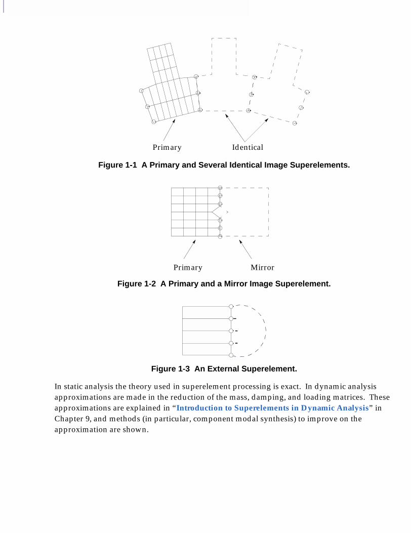
Figure 1-1 A Primary and Several Identical Image Superelements.
Figure 1-2 A Primary and a Mirror Image Superelement.
Figure 1-3 An External Superelement.
In static analysis the theory used in superelement processing is exact. In dynamic analysis approximations are made in the reduction of the mass, damping, and loading matrices. These approximations are explained in “Introduction to Superelements in Dynamic Analysis” in Chapter 9, and methods (in particular, component modal synthesis) to improve on the approximation are shown.
Primary Identical
Primary Mirror
--
-
7CHAPTER 1Introduction and Fundamentals
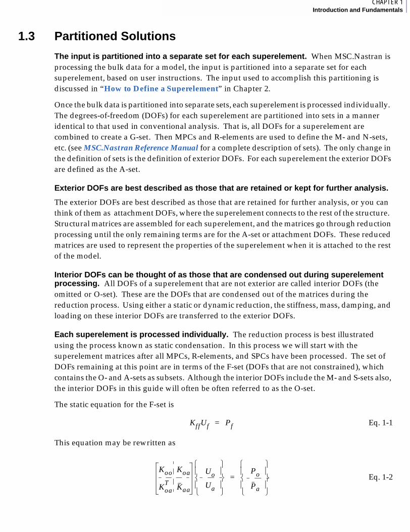
1.3 Partitioned Solutions
The input is partitioned into a separate set for each superelement. When MSC.Nastran is processing the bulk data for a model, the input is partitioned into a separate set for each superelement, based on user instructions. The input used to accomplish this partitioning is discussed in “How to Define a Superelement” in Chapter 2.
Once the bulk data is partitioned into separate sets, each superelement is processed individually. The degrees-of-freedom (DOFs) for each superelement are partitioned into sets in a manner identical to that used in conventional analysis. That is, all DOFs for a superelement are combined to create a G-set. Then MPCs and R-elements are used to define the M- and N-sets, etc. (see MSC.Nastran Reference Manual for a complete description of sets). The only change in the definition of sets is the definition of exterior DOFs. For each superelement the exterior DOFs are defined as the A-set.
Exterior DOFs are best described as those that are retained or kept for further analysis.
The exterior DOFs are best described as those that are retained for further analysis, or you can think of them as attachment DOFs, where the superelement connects to the rest of the structure. Structural matrices are assembled for each superelement, and the matrices go through reduction processing until the only remaining terms are for the A-set or attachment DOFs. These reduced matrices are used to represent the properties of the superelement when it is attached to the rest of the model.
Interior DOFs can be thought of as those that are condensed out during superelement processing. All DOFs of a superelement that are not exterior are called interior DOFs (the omitted or O-set). These are the DOFs that are condensed out of the matrices during the reduction process. Using either a static or dynamic reduction, the stiffness, mass, damping, and loading on these interior DOFs are transferred to the exterior DOFs.
Each superelement is processed individually. The reduction process is best illustrated using the process known as static condensation. In this process we will start with the superelement matrices after all MPCs, R-elements, and SPCs have been processed. The set of DOFs remaining at this point are in terms of the F-set (DOFs that are not constrained), which contains the O- and A-sets as subsets. Although the interior DOFs include the M- and S-sets also, the interior DOFs in this guide will often be often referred to as the O-set.
The static equation for the F-set is
Eq. 1-1
This equation may be rewritten as
Eq. 1-2
KffUf Pf=
Koo Koa
KoaT
Kaa
Uo
Ua
Po
Pa
=
where the bar over a term (for example ) indicates that the sub-matrix represents the associated matrix of terms for that set before the reduction operation. If we look at the upper part of the equation, we obtain
Eq. 1-3
Pre-multiplying both sides of the equation by gives
Eq. 1-4
At this point we will define some terms:
The ‘T’-set is a subset of the ‘A’-set. The ‘T’-set contains any “physical” exterior dof. In static analysis, the ‘T’-set is normally identical to the ‘A’-set. In this part of the book-talking about static analysis-the two will often be used interchangeably.
The static boundary transformation matrix between the exterior and interior motion is called and is defined as
Eq. 1-5
Physically, this matrix represents the solution to the boundary motion problem. That is, each column of this matrix represents the motion of the interior points when one boundary DOF is moved one unit while the other boundary points are held constrained.
Therefore, the transformation matrix has one column for each exterior (boundary) DOF (the A-set for the superelement), and the number of rows are equal to the number of interior DOFs (the O-set for the superelement).
Also, the fixed-boundary displacements of the superelement are defined as follows
Eq. 1-6
This matrix represents the static solution for the displacements of the superelement when the loads are applied and the exterior points are held fixed. Based on these definitions, the total displacement of the interior points can be defined as
Eq. 1-7
where is the solution for the displacements of the exterior (boundary) points. We now substitute the equation for in the lower part of Eq. 1-2, obtaining
Eq. 1-8
From this expression we obtain the reduced stiffness and loading matrices for the superelement. The reduced stiffness, is defined as
Eq. 1-9
Pa
Koo[ ] Uo{ } Koa[ ] Ua{ }+ Po=
Koo[ ] 1–
Uo{ } Koo[ ] 1–Koa[ ] Ua{ }–= Koo[ ] 1–
Po{ }+
Got
Got Koo1–
Kot–=
Uoo
Koo1–
Po=
Uo Uoo
= GotUt+
UtUo
KotT
GotUt Uoo
+[ ] KttUt+ Pt=
Ktt
Ktt KotT
Got= Ktt+

9CHAPTER 1Introduction and Fundamentals
and the reduced loading is defined as
Eq. 1-10
The residual structure consists of all components of the model that were not assigned to any other superelement, plus the assembly of the reduced superelement matrices.
Each superelement is processed in this manner, and its associated matrices are reduced to the exterior DOFs. Once all superelements have been processed, the reduced matrices are assembled into a system matrix during the residual structure processing. The residual structure consists of all components of the model that were not assigned to a superelement, plus the assembly of the reduced superelement matrices.
The system or assembly solution is performed using the assembled matrices for the residual structure. Once the assembly solution is known, the boundary solution is found for each superelement. This boundary solution is used to calculate the interior displacements for each superelement, then standard data recovery is available for all superelements, including the residual structure. Any output that is available in standard (non-superelement) analysis is available in superelement analysis. The difference is that the output is now partitioned by superelement.
Pt
Pt GotT
Po= Pt+
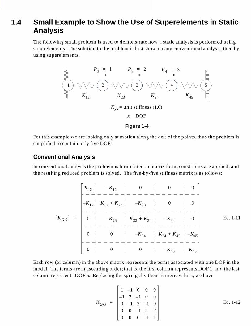
1.4 Small Example to Show the Use of Superelements in Static AnalysisThe following small problem is used to demonstrate how a static analysis is performed using superelements. The solution to the problem is first shown using conventional analysis, then by using superelements.
Figure 1-4
For this example we are looking only at motion along the axis of the points, thus the problem is simplified to contain only five DOFs.
Conventional Analysis
In conventional analysis the problem is formulated in matrix form, constraints are applied, and the resulting reduced problem is solved. The five-by-five stiffness matrix is as follows:
Eq. 1-11
Each row (or column) in the above matrix represents the terms associated with one DOF in the model. The terms are in ascending order; that is, the first column represents DOF 1, and the last column represents DOF 5. Replacing the springs by their numeric values, we have
Eq. 1-12
1 2 3 4 5
P2 1= P3 2= P4 3=
Kxx = unit stiffness (1.0)
K12 K23 K34 K45
x = DOF
KGG[ ]
K12 K12– 0 0 0
K12– K12 K23+ K23– 0 0
0 K23– K23 K34+ K34– 0
0 0 K34– K34 K45+ K45–
0 0 0 K45– K45
=
KGG
1 1– 0 0 01– 2 1– 0 0
0 1– 2 1– 00 0 1– 2 1–
0 0 0 1– 1
=
1CHAPTER 1Introduction and Fundamentals
We now apply the constraints to the problem. In finite element analysis, constraints are applied by removing the associated rows and columns from the matrix; therefore, after applying constraints we have the static equation for the constrained structure
Eq. 1-13
or, in numeric terms
Eq. 1-14
Solving this equation gives the solution
Eq. 1-15
Superelement AnalysisWe now formulate and solve the same problem using superelements, as shown in Figure 1-6. Because the method of defining superelements has not been discussed yet, some of what follows has not been defined. However, as you read further, more of the information will become clear.
First a flowchart showing the order of processing used to perform superelement analysis is shown in Figure 1-5.
U2
U3
U4
K12 K23+ K23–
K23– K23 K34+ K34–
K34 – K34 K45+
1–P2
P3
P4
=
U2
U3
U4
2 1– 0
1– 2 1–
0 1– 2
1–1
2
3
=
U2
U3
U4
2.54.03.5
=
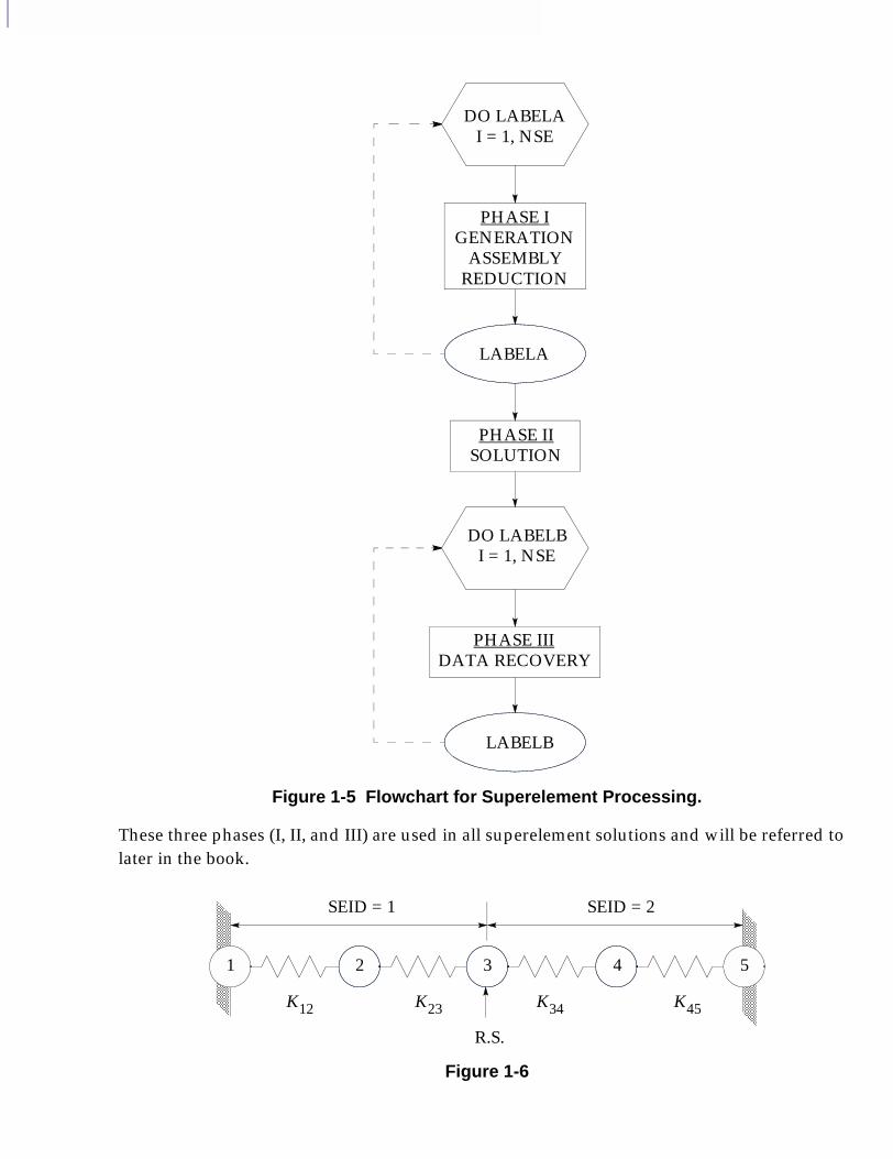
Figure 1-5 Flowchart for Superelement Processing.
These three phases (I, II, and III) are used in all superelement solutions and will be referred to later in the book.
Figure 1-6
DO LABELAI = 1, NSE
PHASE IGENERATION
ASSEMBLYREDUCTION
LABELA
PHASE IISOLUTION
DO LABELBI = 1, NSE
PHASE IIIDATA RECOVERY
LABELB
1 2 3 4 5
R.S.
SEID = 1 SEID = 2
K12 K23 K34 K45
1CHAPTER 1Introduction and Fundamentals
The definitions of the model, as shown previously in Figure 1-6, are as follows:
• Superelement 1 (SEID = 1)
Grid points 1 and 2 are interior points. (These grid points are condensed out during the phase one operations for superelement 1.)
Elements and are interior or belong to superelement 1.
The constraint at grid point 1 is contained in superelement 1.
The load applied on grid point 2 is in superelement 1.
Grid point 3 is exterior to superelement 1. (After all reduction [Phase 1] is completed for superelement 1, all that remains is a set of matrices representing the superelement attached to grid point 3.)
• Superelement 2 (SEID = 2)
Grid points 4 and 5 are interior to superelement 2.
Grid point 3 is exterior to superelement 2.
The load on grid point 4 is in superelement 2.
Elements and are interior to or belong to superelement 2.
The constraint on grid point 5 is contained in superelement 2.
• Residual structure (R.S. OR SEID = 0)
Grid point 3 is interior to the residual structure.
There are no elements left to belong to the residual structure.
The load on grid point 3 is in the residual structure.
Superelements 1 and 2 are processed independently, then the reduced matrices are assembled at the residual.
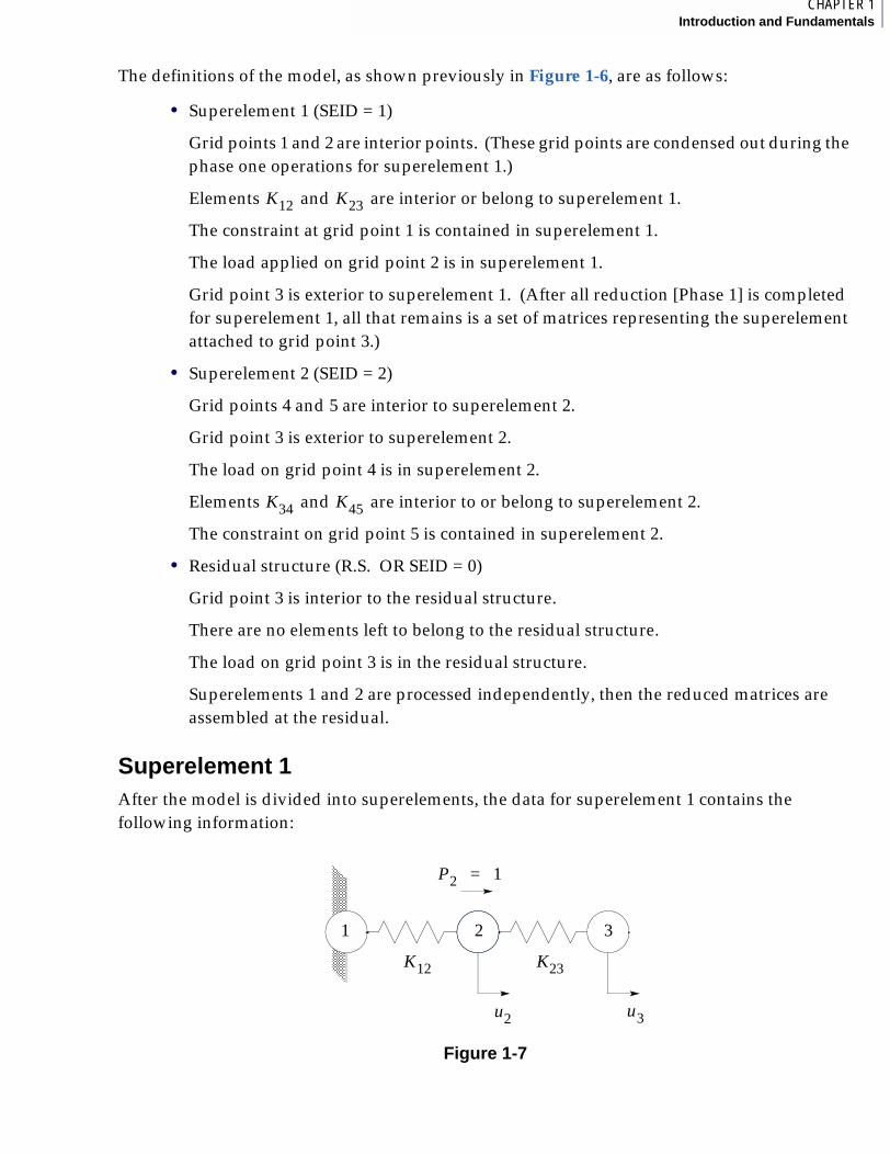
Superelement 1After the model is divided into superelements, the data for superelement 1 contains the following information:
Figure 1-7
K12 K23
K34 K45
1 2 3
P2 1=
K12 K23
u2 u3
Based on this model, is the exterior DOF and belongs to the A-set for superelement 1. Therefore, we want to generate matrices for superelement 1, apply any constraints, and reduce the matrices to the exterior DOF. The G-set for this superelement consists of the DOFs associated with grid points 1, 2, and 3. The following are the G-sized matrices:
Eq. 1-16
Eq. 1-17
The superscript 1 shown on the matrices indicates that they belong to superelement 1. Notice that the force on grid point 3 is not included. Because the force is applied to an exterior point, it is not included in the superelement. This fact is indicated in the matrix for the loading by placing a bar over the term and indicating that this represents only loading on grid point 3 associated with superelement 1.
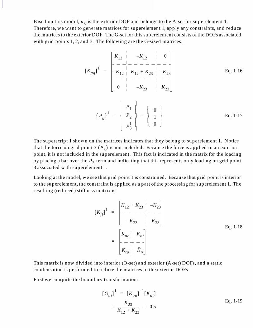
Looking at the model, we see that grid point 1 is constrained. Because that grid point is interior to the superelement, the constraint is applied as a part of the processing for superelement 1. The resulting (reduced) stiffness matrix is
Eq. 1-18
This matrix is now divided into interior (O-set) and exterior (A-set) DOFs, and a static condensation is performed to reduce the matrices to the exterior DOFs.
First we compute the boundary transformation:
Eq. 1-19
u3
Kgg[ ] 1
K12 K12– 0
K12– K12 K23+ K23–
0 K23– K23
=
Pg{ } 1P1
P2
P31
010
= =
P3( )
P3
Kff[ ] 1K12 K23+ K23–
K23– K23
=
Koo Kot
Kto Ktt
=
Got[ ] 1Koo[ ] 1–
Kot[ ]=
K23K12 K23+--------------------------= 0.5=
1CHAPTER 1Introduction and Fundamentals
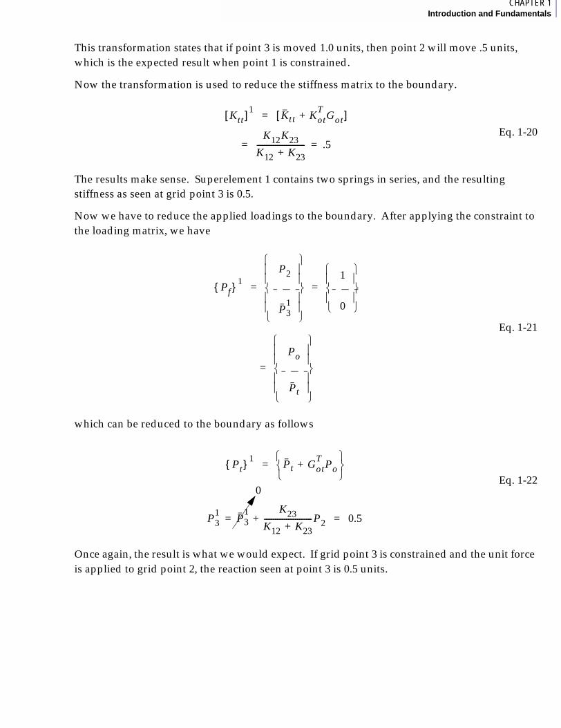
This transformation states that if point 3 is moved 1.0 units, then point 2 will move .5 units, which is the expected result when point 1 is constrained.
Now the transformation is used to reduce the stiffness matrix to the boundary.
Eq. 1-20
The results make sense. Superelement 1 contains two springs in series, and the resulting stiffness as seen at grid point 3 is 0.5.
Now we have to reduce the applied loadings to the boundary. After applying the constraint to the loading matrix, we have
Eq. 1-21
which can be reduced to the boundary as follows
Eq. 1-22
Once again, the result is what we would expect. If grid point 3 is constrained and the unit force is applied to grid point 2, the reaction seen at point 3 is 0.5 units.
Ktt[ ] 1Ktt Kot
TGot+[ ]=
K12K23K12 K23+-------------------------- .5==
Pf{ } 1P2
P31
1 0
= =
Po
Pt
=
Pt{ } 1Pt Got
TPo+
=
P31
P31
=K23
K12 K23+--------------------------P2+ 0.5=
0
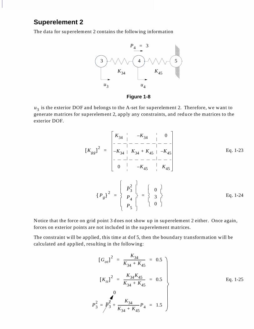
Superelement 2The data for superelement 2 contains the following information
Figure 1-8
is the exterior DOF and belongs to the A-set for superelement 2. Therefore, we want to generate matrices for superelement 2, apply any constraints, and reduce the matrices to the exterior DOF.
Eq. 1-23
Eq. 1-24
Notice that the force on grid point 3 does not show up in superelement 2 either. Once again, forces on exterior points are not included in the superelement matrices.
The constraint will be applied, this time at dof 5, then the boundary transformation will be calculated and applied, resulting in the following:
Eq. 1-25
3 4 5
P4 3=
K34 K45
u3 u4
u3
Kgg[ ] 2
K34 K34– 0
K34– K34 K45+ K45–
0 K45– K45
=
Pg{ } 2P3
2
P4
P5
030
= =
Got[ ] 2 K34K34 K45+-------------------------- 0.5= =
Ktt[ ] 2 K34K45K34 K45+-------------------------- 0.5= =
P32
P32
=K34
K34 K45+--------------------------P4+ 1.5=
0
1CHAPTER 1Introduction and Fundamentals
The transformation and reduced matrices make sense. If grid point 3 is moved 1.0 unit, grid point 4 will move 0.5 units. As before, the stiffness is two springs in series, resulting in a combined stiffness of 0.5, and the load of 3.0 units at grid point 4 gives a 1.5 unit reaction at point 3 if it is constrained.
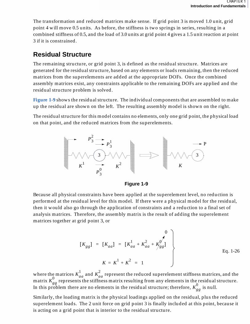
Residual StructureThe remaining structure, or grid point 3, is defined as the residual structure. Matrices are generated for the residual structure, based on any elements or loads remaining, then the reduced matrices from the superelements are added at the appropriate DOFs. Once the combined assembly matrices exist, any constraints applicable to the remaining DOFs are applied and the residual structure problem is solved.
Figure 1-9 shows the residual structure. The individual components that are assembled to make up the residual are shown on the left. The resulting assembly model is shown on the right.
The residual structure for this model contains no elements, only one grid point, the physical load on that point, and the reduced matrices from the superelements.
Figure 1-9
Because all physical constraints have been applied at the superelement level, no reduction is performed at the residual level for this model. If there were a physical model for the residual, then it would also go through the application of constraints and a reduction to a final set of analysis matrices. Therefore, the assembly matrix is the result of adding the superelement matrices together at grid point 3, or
Eq. 1-26
where the matrices and represent the reduced superelement stiffness matrices, and the matrix represents the stiffness matrix resulting from any elements in the residual structure. In this problem there are no elements in the residual structure; therefore, is null.
Similarly, the loading matrix is the physical loadings applied on the residual, plus the reduced superelement loads. The 2 unit force on grid point 3 is finally included at this point, because it is acting on a grid point that is interior to the residual structure.
3 3
PP3
2
P31
P30
K1
K2 K
Kgg[ ] Kaa[ ] Kaa1
Kaa2
Kgg0
+ +[ ]= =
K K1
= K2
+ 1=
0
Kaa1
Kaa2
Kgg0
Kgg0
Eq. 1-27
Eq. 1-28
Now that the stiffness and loading matrices have been generated and reduced, we are ready to solve the residual structure problem for the A-set displacements
Eq. 1-29
Eq. 1-30
We now have the displacement solution for the residual structure, and we are ready to begin data recovery. Data recovery is processed for each superelement independently, allowing segmented or selective data recovery.
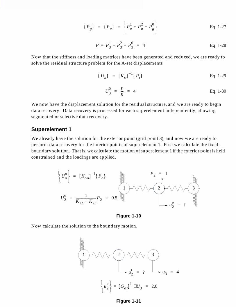
Superelement 1
We already have the solution for the exterior point (grid point 3), and now we are ready to perform data recovery for the interior points of superelement 1. First we calculate the fixed-boundary solution. That is, we calculate the motion of superelement 1 if the exterior point is held constrained and the loadings are applied.
Figure 1-10
Now calculate the solution to the boundary motion.
Figure 1-11
Pg{ } Pa{ } Pa1
Pa2
Pg0
+ +
= =
P P31
= P32
P30
+ + 4=
Ua{ } Ktt[ ] 1–Pt{ }=
U30 P
K---- 4= =
1 2 3
Uoo
Koo[ ] 1–Po{ }=
U2o 1
K12 K23+-------------------------- P2 0.5= =
P2 1=
u2o ?=
1 2 3
u2t ?= u3 4=
u2a
Got[ ] 1= U3⋅ 2.0=
1CHAPTER 1Introduction and Fundamentals
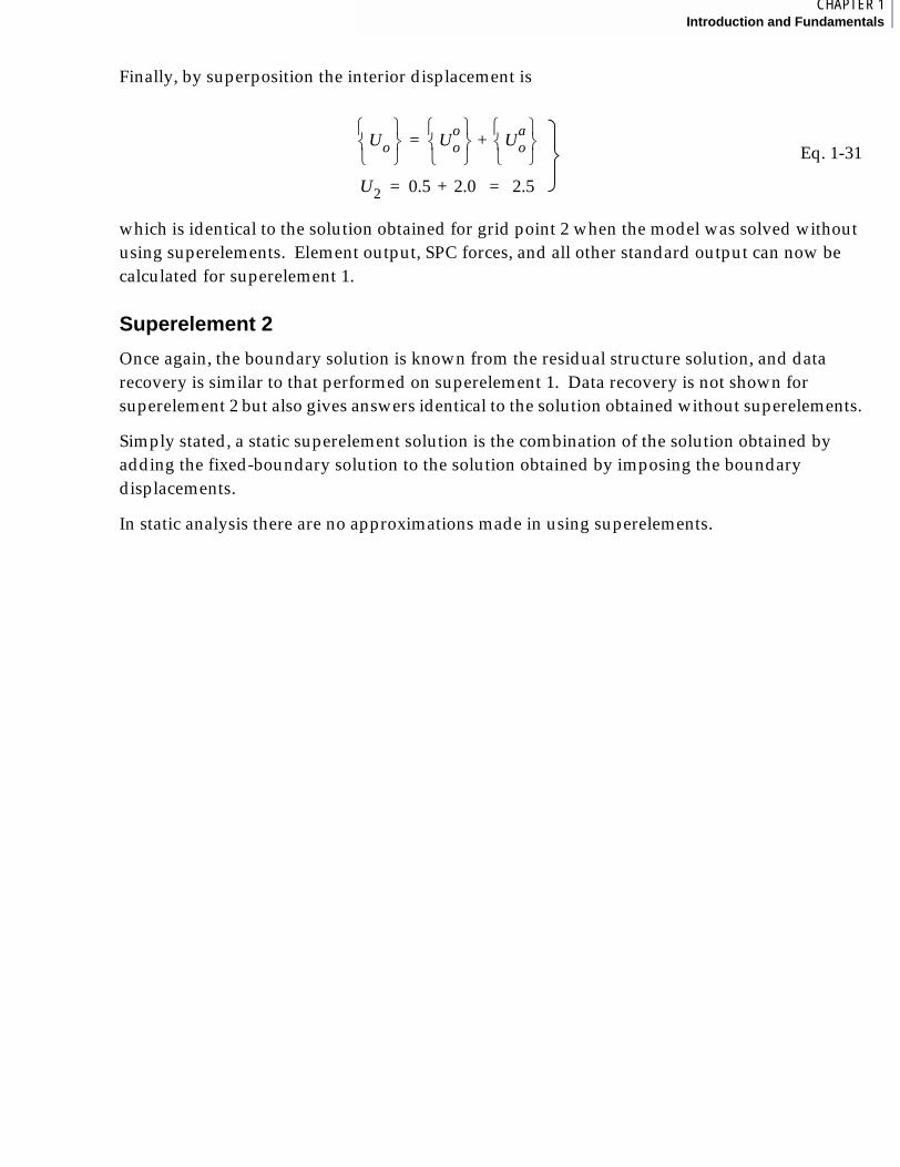
Finally, by superposition the interior displacement is
Eq. 1-31
which is identical to the solution obtained for grid point 2 when the model was solved without using superelements. Element output, SPC forces, and all other standard output can now be calculated for superelement 1.
Superelement 2
Once again, the boundary solution is known from the residual structure solution, and data recovery is similar to that performed on superelement 1. Data recovery is not shown for superelement 2 but also gives answers identical to the solution obtained without superelements.
Simply stated, a static superelement solution is the combination of the solution obtained by adding the fixed-boundary solution to the solution obtained by imposing the boundary displacements.
In static analysis there are no approximations made in using superelements.
Uo
Uoo
= Uoa
+
U2 0.5= 2.0+ 2.5=
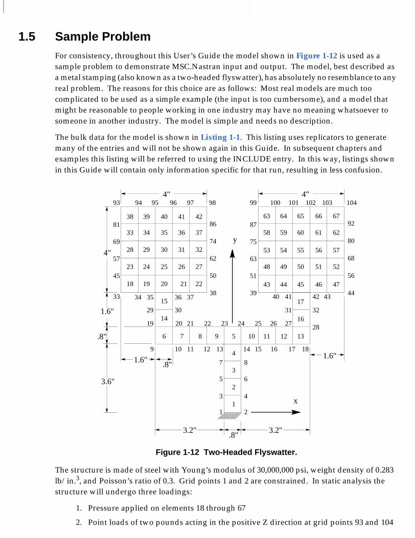
1.5 Sample ProblemFor consistency, throughout this User’s Guide the model shown in Figure 1-12 is used as a sample problem to demonstrate MSC.Nastran input and output. The model, best described as a metal stamping (also known as a two-headed flyswatter), has absolutely no resemblance to any real problem. The reasons for this choice are as follows: Most real models are much too complicated to be used as a simple example (the input is too cumbersome), and a model that might be reasonable to people working in one industry may have no meaning whatsoever to someone in another industry. The model is simple and needs no description.
The bulk data for the model is shown in Listing 1-1. This listing uses replicators to generate many of the entries and will not be shown again in this Guide. In subsequent chapters and examples this listing will be referred to using the INCLUDE entry. In this way, listings shown in this Guide will contain only information specific for that run, resulting in less confusion.
Figure 1-12 Two-Headed Flyswatter.
The structure is made of steel with Young’s modulus of 30,000,000 psi, weight density of 0.283 lb/in.3, and Poisson’s ratio of 0.3. Grid points 1 and 2 are constrained. In static analysis the structure will undergo three loadings:
1. Pressure applied on elements 18 through 67
2. Point loads of two pounds acting in the positive Z direction at grid points 93 and 104
4" 4"
4"
1.6"
1.6" 1.6".8"
.8"
.8"3.2" 3.2"
3.6"
93 94 95 96 97 98 99 100 101 102 103 104
38 39 40 41 42
33 34 35 36 37
28 29 30 31 32
23 24 25 26 27
18 19 20 21 22
63 64 65 66 67
58 59 60 61 62
53 54 55 56 57
48 49 50 51 52
43 44 45
17
16
13
46 47
81
69
57
45
33
86
74
62
50
38
87
75
63
51
39
92
80
68
56
4434 35 36 37 40 41 42 43
15
14
6
9 10 11 12 13 14 15 16 17 18
19 20 21 22 23 24 25 26 27 28
29 30 31 32
1
2
3
4
5
6
7 8
1 2
3 4
5
7 8 9 10 11 12
y
x

2CHAPTER 1Introduction and Fundamentals
3. Opposing two pound point loads in the Z direction at grid points 93 and 104.
Listing 1-1 Listing of Bulk Data for the Sample Problem.
$$ **************************************************************$ BASIC MODEL DEFINITION - SAME FOR ALL RUNS$ **************************************************************$$ FILE NAME IS MODEL.DAT$GRDSET,,,,,,,6GRID,1,,-.4,0.,0.,,123456GRID,3,,-.4,0.9,0.=,*2,=,=,*.9,===1GRID,2,,.4,0.,0.,,123456GRID,4,,.4,0.9,0.=,*2,=,=,*.9,===1GRID,9,,-3.6,3.6,0.=,*1,=,*.8,===8GRID,19,,-3.6,4.4,0.=,*1,=,*.8,===8GRID,29,,-3.6,5.2,0.GRID,30,,-2.8,5.2,0.GRID,31,,2.8,5.2,0.GRID,32,,3.6,5.2,0.GRID,33,,-5.2,6.,0.=,*1,=,*.8,===4GRID,39,,1.2,6.,0.=,*1,=,*.8,===4GRID,45,,-5.2,6.8,0.=,*1,=,*.8,===4GRID,51,,1.2,6.8,0.=,*1,=,*.8,===4GRID,57,,-5.2,7.6,0.=,*1,=,*.8,===4GRID,63,,1.2,7.6,0.=,*1,=,*.8,===4GRID,69,,-5.2,8.4,0.=,*1,=,*.8,===4GRID,75,,1.2,8.4,0.=,*1,=,*.8,===4GRID,81,,-5.2,9.2,0.=,*1,=,*.8,===4GRID,87,,1.2,9.2,0.=,*1,=,*.8,===4GRID,93,,-5.2,10.,0.=,*1,=,*.8,===4GRID,99,,1.2,10.,0.=,*1,=,*.8,===4$
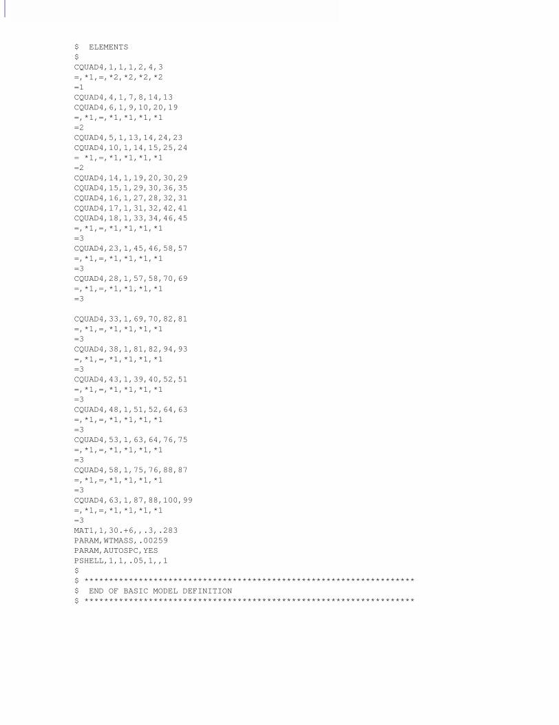
$ ELEMENTS$CQUAD4,1,1,1,2,4,3=,*1,=,*2,*2,*2,*2=1CQUAD4,4,1,7,8,14,13CQUAD4,6,1,9,10,20,19=,*1,=,*1,*1,*1,*1=2CQUAD4,5,1,13,14,24,23CQUAD4,10,1,14,15,25,24= *1,=,*1,*1,*1,*1=2CQUAD4,14,1,19,20,30,29CQUAD4,15,1,29,30,36,35CQUAD4,16,1,27,28,32,31CQUAD4,17,1,31,32,42,41CQUAD4,18,1,33,34,46,45=,*1,=,*1,*1,*1,*1=3CQUAD4,23,1,45,46,58,57=,*1,=,*1,*1,*1,*1=3CQUAD4,28,1,57,58,70,69=,*1,=,*1,*1,*1,*1=3
CQUAD4,33,1,69,70,82,81=,*1,=,*1,*1,*1,*1=3CQUAD4,38,1,81,82,94,93=,*1,=,*1,*1,*1,*1=3CQUAD4,43,1,39,40,52,51=,*1,=,*1,*1,*1,*1=3CQUAD4,48,1,51,52,64,63=,*1,=,*1,*1,*1,*1=3CQUAD4,53,1,63,64,76,75=,*1,=,*1,*1,*1,*1=3CQUAD4,58,1,75,76,88,87=,*1,=,*1,*1,*1,*1=3CQUAD4,63,1,87,88,100,99=,*1,=,*1,*1,*1,*1=3MAT1,1,30.+6,,.3,.283PARAM,WTMASS,.00259PARAM,AUTOSPC,YESPSHELL,1,1,.05,1,,1$$ *******************************************************************$ END OF BASIC MODEL DEFINITION$ *******************************************************************
MSC.Nastran Superelement Users’s Guide
CHAPTER
2 How to Define a Superelement
■ Defining a Superelement Using Partitioned Bulk Data (PARTs)
■ Defining Superelements in the Main Bulk Data Section

Now that the basic concept of superelements has been explained, it is time to learn how to define superelements in MSC.Nastran. Superelements are defined using the Bulk Data Section of the input file. There are two methods available for defining superelements, main bulk data superelements and PARTs.
The residual structure is superelement 0. The following sections provide a description of each method, with examples. Each superelement in MSC.Nastran is identified by an integer identification known as the SEID. Each SEID must be a unique positive integer (with the exception of the residual structure, which is known as superelement 0).
If no superelements are defined, the model is assumed to be a residual-structure-only model, and a conventional (non-superelement) solution is performed. By default, all superelement solutions perform a conventional solution if no superelements are defined.
As the name implies, main bulk data superelements are defined in the Main Bulk Data Section of the input file. When superelements are defined using this approach, the model defined in this section of the input is cut apart into separate components (each component is a superelement). A good way to describe this is to say that the program is using a cookie-cutter approach with the model, taking a complete model and dividing it into superelements.
PART superelements are defined in a different manner. Each superelement is defined in its own Partitioned Bulk Data Section. These separate sections of the bulk data are self-contained in that each section contains all geometry, elements, properties, constraints, and loading data for that component of the model. When PARTs are used the program works in a manner similar to an assembly process. That is, a series of separate components are assembled into the final finite element model.
The two approaches can be used independently or together; the choice is up to you. In versions prior to Version 69, only the main bulk data superelements were available. Input files from versions prior to Version 69 of MSC.Nastran can be used in later versions, and any superelement input will be treated as before. Once PARTs are defined, the program uses a different set of rules to partition the Main Bulk Data Section into superelements.
2CHAPTER 2How to Define a Superelement
2.1 Defining a Superelement Using Partitioned Bulk Data (PARTs)
Defining PARTsPARTs are defined as separate components using separate areas of the Bulk Data Section in MSC.Nastran. Therefore, each PART can be thought of as a separate component model. MSC.Nastran automatically locates any coincident grid points in the PARTs and connects the component models to create the assembly model.
Starting with Version 69, the Bulk Data Section can be divided into separate sections for each PART. This division is accomplished by using the BEGIN SUPER entry. The format of this entry is as follows:
BEGIN [BULK] SUPER = i
where i is the superelement id being defined. The commonly used form of this command is:
BEGIN SUPER = i
which is the form used in this book.
Prior to Version 69, the Bulk Data Section of the input file was a single section of data with the exception of auxmodels in optimization, which contained the complete model definition. The entire model was defined in the area between BEGIN BULK and ENDDATA. Each grid point had to be unique, and each element id had to be unique. Beginning with Version 69, it became possible to partition the Bulk Data Section of the input into separate component models, using the BEGIN SUPER command. Thus, each of these component models is a self-contained model defining a PART of the total model. Within each of these sections, grid point and element ids must be unique as before; however, different PARTs can reuse grid and element ids, because the sections are separate in the input file.
The Bulk Data Section Using PARTsWhen PARTs are used, the bulk data is divided into different sections. The section of the bulk data contained between the BEGIN BULK and either the first BEGIN SUPER or the ENDDATA is known as the Main Bulk Data Section. If only this area is used, then the file is compatible with versions of MSC.Nastran prior to Version 69. In this section superelements can be defined (although it is not required) using the method shown in “Defining Superelements in the Main Bulk Data Section” on page 46. Any superelements defined in this section are known as main bulk data superelements.
When you define PARTS it is not necessary for you to tell MSC.Nastran where to make the connections to other superelements. The program contains logic to determine which grid points are coincident and will (by default) automatically connect any coincident grid points. Later in this section we will discuss how to override the automatic connection.

Format of the Input File When PARTs Are UsedWhen PARTs are used the Executive and Case Control Sections are unchanged, only the Bulk Data Section is different. A sample input file looks like the following:
SOL 101 CENDTITLE = Sample Input File Demonstrating PARTs..BEGIN BULK$$ MAIN BULK DATA SECTION$..BEGIN SUPER = 1$$ data for PART 1$..BEGIN SUPER = 25$$ data for PART 25$..ENDDATA
In this example, there is a Main Bulk Data Section (in which you can define some main bulk data superelements) and two PART superelements (1 and 25). Each section is self-contained. That is, no entry in PART 1 can reference an entry in any other section of the input. This goes for all PARTs; they must be self-contained. There are several main bulk data entries that can be used to move, copy, or manually connect PARTs, but beyond these entries, no entry in any section of the input can reference an entry in any other section of the bulk data.
We will look at how to define the two-headed flyswatter model (from the previous section) using PARTs. We are going to define the model using seven PART superelements and a residual structure. The following figure shows how the model will be divided into superelements.
2CHAPTER 2How to Define a Superelement
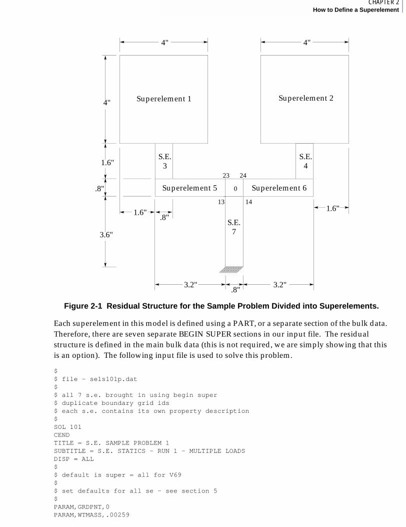
Figure 2-1 Residual Structure for the Sample Problem Divided into Superelements.
Each superelement in this model is defined using a PART, or a separate section of the bulk data. Therefore, there are seven separate BEGIN SUPER sections in our input file. The residual structure is defined in the main bulk data (this is not required, we are simply showing that this is an option). The following input file is used to solve this problem.
$$ file - se1s101p.dat$ $ all 7 s.e. brought in using begin super$ duplicate boundary grid ids$ each s.e. contains its own property description$SOL 101 CENDTITLE = S.E. SAMPLE PROBLEM 1 SUBTITLE = S.E. STATICS - RUN 1 - MULTIPLE LOADSDISP = ALL$$ default is super = all for V69$$ set defaults for all se - see section 5$PARAM,GRDPNT,0PARAM,WTMASS,.00259
4" 4"
4"
1.6"
1.6" 1.6".8"
.8"
.8"3.2" 3.2"
3.6"
13 14
23 24
0
Superelement 1 Superelement 2
S.E.3
S.E.4
Superelement 5 Superelement 6
S.E.7
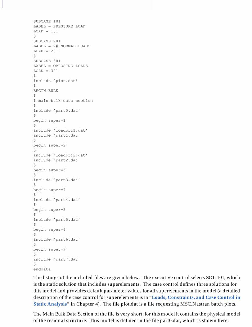
SUBCASE 101LABEL = PRESSURE LOADLOAD = 101$SUBCASE 201LABEL = 2# NORMAL LOADSLOAD = 201$SUBCASE 301LABEL = OPPOSING LOADSLOAD = 301$include ’plot.dat’$BEGIN BULK$$ main bulk data section$include ’part0.dat’$begin super=1$include ’loadprt1.dat’include ’part1.dat’$begin super=2$ include ’loadprt2.dat’include ’part2.dat’$begin super=3$ include ’part3.dat’$begin super=4$ include ’part4.dat’$begin super=5$ include ’part5.dat’$begin super=6$ include ’part6.dat’$begin super=7$ include ’part7.dat’$enddata
The listings of the included files are given below. The executive control selects SOL 101, which is the static solution that includes superelements. The case control defines three solutions for this model and provides default parameter values for all superelements in the model (a detailed description of the case control for superelements is in “Loads, Constraints, and Case Control in Static Analysis” in Chapter 4). The file plot.dat is a file requesting MSC.Nastran batch plots.
The Main Bulk Data Section of the file is very short; for this model it contains the physical model of the residual structure. This model is defined in the file part0.dat, which is shown here:
2CHAPTER 2How to Define a Superelement
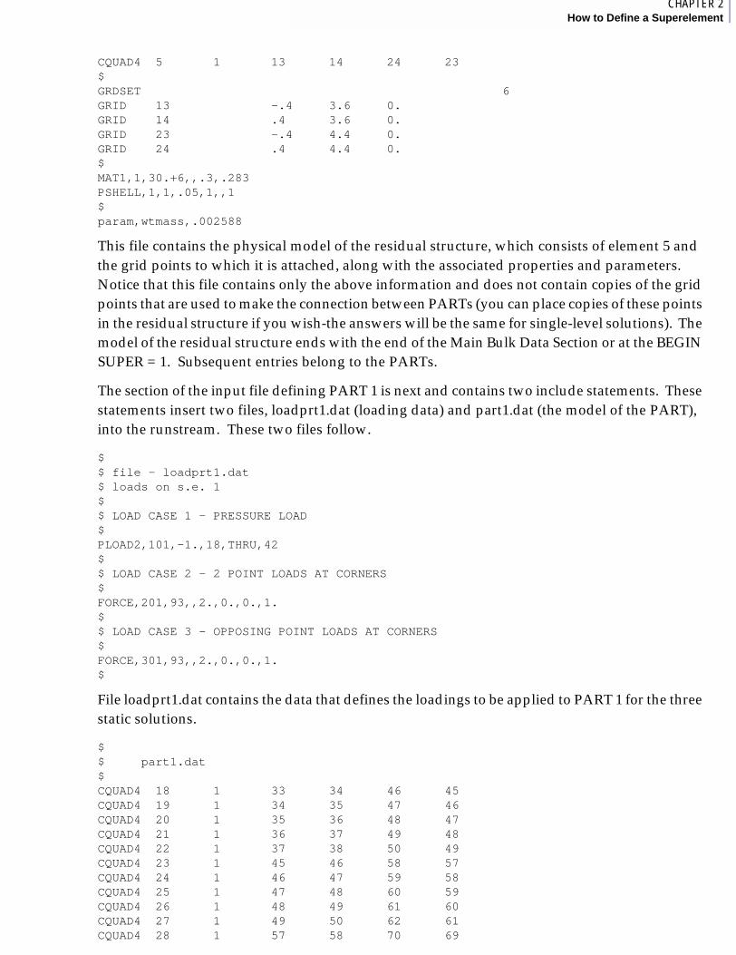
CQUAD4 5 1 13 14 24 23 $GRDSET 6 GRID 13 -.4 3.6 0. GRID 14 .4 3.6 0. GRID 23 -.4 4.4 0. GRID 24 .4 4.4 0. $MAT1,1,30.+6,,.3,.283PSHELL,1,1,.05,1,,1$param,wtmass,.002588
This file contains the physical model of the residual structure, which consists of element 5 and the grid points to which it is attached, along with the associated properties and parameters. Notice that this file contains only the above information and does not contain copies of the grid points that are used to make the connection between PARTs (you can place copies of these points in the residual structure if you wish-the answers will be the same for single-level solutions). The model of the residual structure ends with the end of the Main Bulk Data Section or at the BEGIN SUPER = 1. Subsequent entries belong to the PARTs.
The section of the input file defining PART 1 is next and contains two include statements. These statements insert two files, loadprt1.dat (loading data) and part1.dat (the model of the PART), into the runstream. These two files follow.
$$ file - loadprt1.dat$ loads on s.e. 1$$ LOAD CASE 1 - PRESSURE LOAD$PLOAD2,101,-1.,18,THRU,42$$ LOAD CASE 2 - 2 POINT LOADS AT CORNERS$FORCE,201,93,,2.,0.,0.,1.$$ LOAD CASE 3 - OPPOSING POINT LOADS AT CORNERS$FORCE,301,93,,2.,0.,0.,1.$
File loadprt1.dat contains the data that defines the loadings to be applied to PART 1 for the three static solutions.
$$ part1.dat$ CQUAD4 18 1 33 34 46 45 CQUAD4 19 1 34 35 47 46 CQUAD4 20 1 35 36 48 47 CQUAD4 21 1 36 37 49 48 CQUAD4 22 1 37 38 50 49 CQUAD4 23 1 45 46 58 57 CQUAD4 24 1 46 47 59 58 CQUAD4 25 1 47 48 60 59 CQUAD4 26 1 48 49 61 60 CQUAD4 27 1 49 50 62 61 CQUAD4 28 1 57 58 70 69
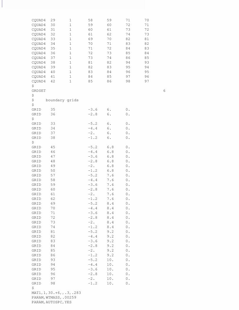
CQUAD4 29 1 58 59 71 70 CQUAD4 30 1 59 60 72 71 CQUAD4 31 1 60 61 73 72 CQUAD4 32 1 61 62 74 73 CQUAD4 33 1 69 70 82 81 CQUAD4 34 1 70 71 83 82 CQUAD4 35 1 71 72 84 83 CQUAD4 36 1 72 73 85 84 CQUAD4 37 1 73 74 86 85 CQUAD4 38 1 81 82 94 93 CQUAD4 39 1 82 83 95 94 CQUAD4 40 1 83 84 96 95 CQUAD4 41 1 84 85 97 96 CQUAD4 42 1 85 86 98 97 $GRDSET 6 $$ boundary grids$GRID 35 -3.6 6. 0. GRID 36 -2.8 6. 0. $GRID 33 -5.2 6. 0. GRID 34 -4.4 6. 0. GRID 37 -2. 6. 0. GRID 38 -1.2 6. 0. $GRID 45 -5.2 6.8 0. GRID 46 -4.4 6.8 0. GRID 47 -3.6 6.8 0. GRID 48 -2.8 6.8 0. GRID 49 -2. 6.8 0. GRID 50 -1.2 6.8 0. GRID 57 -5.2 7.6 0. GRID 58 -4.4 7.6 0. GRID 59 -3.6 7.6 0. GRID 60 -2.8 7.6 0. GRID 61 -2. 7.6 0. GRID 62 -1.2 7.6 0. GRID 69 -5.2 8.4 0. GRID 70 -4.4 8.4 0. GRID 71 -3.6 8.4 0. GRID 72 -2.8 8.4 0. GRID 73 -2. 8.4 0. GRID 74 -1.2 8.4 0. GRID 81 -5.2 9.2 0. GRID 82 -4.4 9.2 0. GRID 83 -3.6 9.2 0. GRID 84 -2.8 9.2 0. GRID 85 -2. 9.2 0. GRID 86 -1.2 9.2 0. GRID 93 -5.2 10. 0. GRID 94 -4.4 10. 0. GRID 95 -3.6 10. 0. GRID 96 -2.8 10. 0. GRID 97 -2. 10. 0. GRID 98 -1.2 10. 0. $MAT1,1,30.+6,,.3,.283PARAM,WTMASS,.00259PARAM,AUTOSPC,YES
3CHAPTER 2How to Define a Superelement
PSHELL,1,1,.05,1,,1$
File part1.dat contains the physical model for PART1. If you look at the illustration of the model provided in the previous section, you will notice that this PART attaches to PART 3 at grid points 35 and 36. Notice that these points are contained in the data for this component of the model.
PART 2 is defined by similar files (shown later in this section) and will not be discussed here.
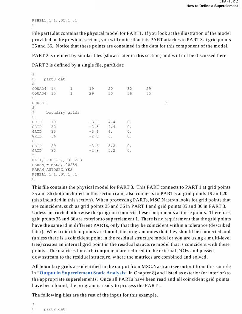
PART 3 is defined by a single file, part3.dat:
$$ part3.dat$ CQUAD4 14 1 19 20 30 29 CQUAD4 15 1 29 30 36 35 $GRDSET 6 $$ boundary grids$GRID 19 -3.6 4.4 0. GRID 20 -2.8 4.4 0. GRID 35 -3.6 6. 0. GRID 36 -2.8 6. 0. $GRID 29 -3.6 5.2 0. GRID 30 -2.8 5.2 0. $MAT1,1,30.+6,,.3,.283PARAM,WTMASS,.00259PARAM,AUTOSPC,YESPSHELL,1,1,.05,1,,1$
This file contains the physical model for PART 3. This PART connects to PART 1 at grid points 35 and 36 (both included in this section) and also connects to PART 5 at grid points 19 and 20 (also included in this section). When processing PARTs, MSC.Nastran looks for grid points that are coincident, such as grid points 35 and 36 in PART 1 and grid points 35 and 36 in PART 3. Unless instructed otherwise the program connects these components at these points. Therefore, grid points 35 and 36 are exterior to superelement 1. There is no requirement that the grid points have the same id in different PARTs, only that they be coincident within a tolerance (described later). When coincident points are found, the program notes that they should be connected and (unless there is a coincident point in the residual structure model or you are using a multi-level tree) creates an internal grid point in the residual structure model that is coincident with these points. The matrices for each component are reduced to the external DOFs and passed downstream to the residual structure, where the matrices are combined and solved.
All boundary grids are identified in the output from MSC.Nastran (see output from this sample in “Output in Superelement Static Analysis” in Chapter 8) and listed as exterior (or interior) to the appropriate superelements. Once all PARTs have been read and all coincident grid points have been found, the program is ready to process the PARTs.
The following files are the rest of the input for this example.
$ $ part2.dat
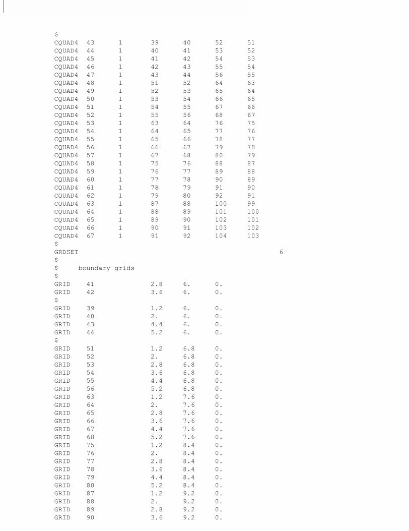
$CQUAD4 43 1 39 40 52 51 CQUAD4 44 1 40 41 53 52 CQUAD4 45 1 41 42 54 53 CQUAD4 46 1 42 43 55 54 CQUAD4 47 1 43 44 56 55 CQUAD4 48 1 51 52 64 63 CQUAD4 49 1 52 53 65 64 CQUAD4 50 1 53 54 66 65 CQUAD4 51 1 54 55 67 66 CQUAD4 52 1 55 56 68 67 CQUAD4 53 1 63 64 76 75 CQUAD4 54 1 64 65 77 76 CQUAD4 55 1 65 66 78 77 CQUAD4 56 1 66 67 79 78 CQUAD4 57 1 67 68 80 79 CQUAD4 58 1 75 76 88 87 CQUAD4 59 1 76 77 89 88 CQUAD4 60 1 77 78 90 89 CQUAD4 61 1 78 79 91 90 CQUAD4 62 1 79 80 92 91 CQUAD4 63 1 87 88 100 99 CQUAD4 64 1 88 89 101 100 CQUAD4 65 1 89 90 102 101 CQUAD4 66 1 90 91 103 102 CQUAD4 67 1 91 92 104 103 $GRDSET 6 $$ boundary grids$GRID 41 2.8 6. 0. GRID 42 3.6 6. 0. $GRID 39 1.2 6. 0. GRID 40 2. 6. 0. GRID 43 4.4 6. 0. GRID 44 5.2 6. 0. $GRID 51 1.2 6.8 0. GRID 52 2. 6.8 0. GRID 53 2.8 6.8 0. GRID 54 3.6 6.8 0. GRID 55 4.4 6.8 0. GRID 56 5.2 6.8 0. GRID 63 1.2 7.6 0. GRID 64 2. 7.6 0. GRID 65 2.8 7.6 0. GRID 66 3.6 7.6 0. GRID 67 4.4 7.6 0. GRID 68 5.2 7.6 0. GRID 75 1.2 8.4 0. GRID 76 2. 8.4 0. GRID 77 2.8 8.4 0. GRID 78 3.6 8.4 0. GRID 79 4.4 8.4 0. GRID 80 5.2 8.4 0. GRID 87 1.2 9.2 0. GRID 88 2. 9.2 0. GRID 89 2.8 9.2 0. GRID 90 3.6 9.2 0.
3CHAPTER 2How to Define a Superelement
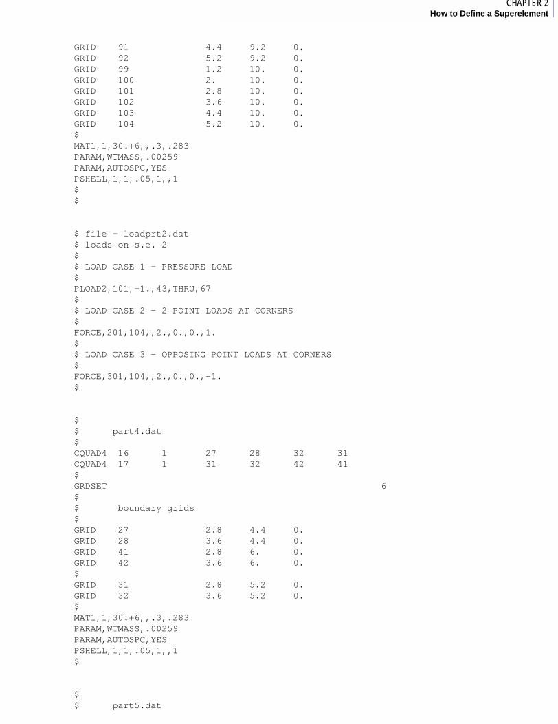
GRID 91 4.4 9.2 0. GRID 92 5.2 9.2 0. GRID 99 1.2 10. 0. GRID 100 2. 10. 0. GRID 101 2.8 10. 0. GRID 102 3.6 10. 0. GRID 103 4.4 10. 0. GRID 104 5.2 10. 0. $MAT1,1,30.+6,,.3,.283PARAM,WTMASS,.00259PARAM,AUTOSPC,YESPSHELL,1,1,.05,1,,1$$
$ file - loadprt2.dat$ loads on s.e. 2 $$ LOAD CASE 1 - PRESSURE LOAD$PLOAD2,101,-1.,43,THRU,67$$ LOAD CASE 2 - 2 POINT LOADS AT CORNERS$FORCE,201,104,,2.,0.,0.,1.$$ LOAD CASE 3 - OPPOSING POINT LOADS AT CORNERS$FORCE,301,104,,2.,0.,0.,-1.$
$$ part4.dat$ CQUAD4 16 1 27 28 32 31 CQUAD4 17 1 31 32 42 41 $GRDSET 6 $$ boundary grids$GRID 27 2.8 4.4 0. GRID 28 3.6 4.4 0. GRID 41 2.8 6. 0. GRID 42 3.6 6. 0. $GRID 31 2.8 5.2 0. GRID 32 3.6 5.2 0. $MAT1,1,30.+6,,.3,.283PARAM,WTMASS,.00259PARAM,AUTOSPC,YESPSHELL,1,1,.05,1,,1$
$ $ part5.dat
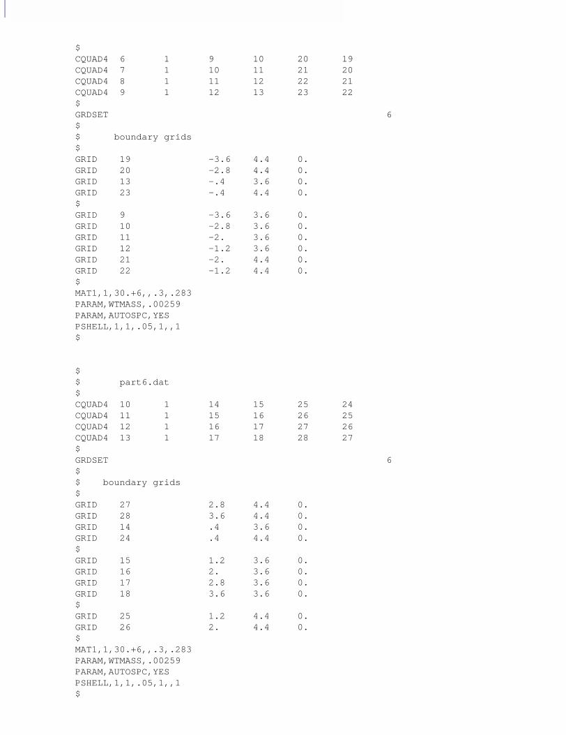
$CQUAD4 6 1 9 10 20 19 CQUAD4 7 1 10 11 21 20 CQUAD4 8 1 11 12 22 21 CQUAD4 9 1 12 13 23 22 $GRDSET 6 $$ boundary grids$GRID 19 -3.6 4.4 0. GRID 20 -2.8 4.4 0. GRID 13 -.4 3.6 0. GRID 23 -.4 4.4 0. $GRID 9 -3.6 3.6 0. GRID 10 -2.8 3.6 0. GRID 11 -2. 3.6 0. GRID 12 -1.2 3.6 0. GRID 21 -2. 4.4 0. GRID 22 -1.2 4.4 0. $MAT1,1,30.+6,,.3,.283PARAM,WTMASS,.00259PARAM,AUTOSPC,YESPSHELL,1,1,.05,1,,1$
$ $ part6.dat$CQUAD4 10 1 14 15 25 24 CQUAD4 11 1 15 16 26 25 CQUAD4 12 1 16 17 27 26 CQUAD4 13 1 17 18 28 27 $GRDSET 6 $$ boundary grids$GRID 27 2.8 4.4 0. GRID 28 3.6 4.4 0. GRID 14 .4 3.6 0. GRID 24 .4 4.4 0. $GRID 15 1.2 3.6 0. GRID 16 2. 3.6 0. GRID 17 2.8 3.6 0. GRID 18 3.6 3.6 0. $GRID 25 1.2 4.4 0. GRID 26 2. 4.4 0. $MAT1,1,30.+6,,.3,.283PARAM,WTMASS,.00259PARAM,AUTOSPC,YESPSHELL,1,1,.05,1,,1$

3CHAPTER 2How to Define a Superelement
$ $ part7.dat$CQUAD4 1 1 1 2 4 3 CQUAD4 2 1 3 4 6 5 CQUAD4 3 1 5 6 8 7 CQUAD4 4 1 7 8 14 13 $GRDSET 6 $GRID 1 -.4 0. 0. 123456 GRID 2 .4 0. 0. 123456 GRID 3 -.4 0.9 0. GRID 4 .4 0.9 0. GRID 5 -.4 1.8 0. GRID 6 .4 1.8 0. GRID 7 -.4 2.7 0. GRID 8 .4 2.7 0. $$ boundary grids$GRID 13 -.4 3.6 0. GRID 14 .4 3.6 0. $MAT1,1,30.+6,,.3,.283PARAM,WTMASS,.00259PARAM,AUTOSPC,YESPSHELL,1,1,.05,1,,1$
Automatically Connecting PARTs to Other Components of the ModelBy default, the program automatically connects points from a PART to any coincident points in any other PARTs or in the Main Bulk Data Section. There is no need to be concerned with coordinate systems on these coincident points; MSC.Nastran automatically connects coincident points, accounting for differences in the output coordinate systems.
These points will be identified as boundary points in the output from MSC.Nastran. By default, no special effort is required from you to make the connection. If for one connection all the boundary points belong to PARTs (none of the coincident points are in the residual structure), then MSC.Nastran will create a new point internally that is coincident with the boundary points and place that internal point in the residual structure (or the lowest connected superelement in a multi-level tree). These internal points can not be constrained. If you wish to apply a constraint on this point, you can define a coincident grid point in the residual structure (or in the lowest connected superelement for a multi-level tree) and constrain that point, or you can apply constraints in the PARTs (subject to the limitations in the next paragraph).
Constraints on Connecting PointsIf you need to apply constraints on the points where two or more PARTs connect, there are limitations. If you wish to constrain all six DOFs, there is no limitation; place the constraint on the connecting grid point in any of the PARTs and all other coincident points are also constrained in all six DOFs. If the constraint is not on all six DOFs, then you must exercise care. Because the program will allow the connection of coincident points that have different output

coordinate systems, it would be difficult to allow constraints on one of the points in one coordinate system and to correctly map that set of constraints onto another system. Therefore, the following set of rules is enforced at connecting points:
If the PARTs being connected are at the same level in the superelement tree, either all six or none of the DOFs must be constrained.
If one of the PARTs is at a lower level in the tree, then you must apply the desired constraints at the connection inside the PART that is lowest in the processing tree (last of the group to be processed).
Controlling the Connection Between PARTs and the Rest of the Model
The SEBNDRY, SEBULK, SECONCT, and SEEXCLD entries can appear only in the Main Bulk Data Section of your input file. If you wish to override the automatic connection, there are several options available to you. You can control this operation by using the SEBNDRY, SEBULK, SECONCT, and SEEXCLD entries in the Main Bulk Data Section of your input file.
Although a more thorough explanation follows, here is a quick definition of each of these entries:
The default tolerance in the coincident grid search logic is 1.0E-5 units. By default, MSC.Nastran uses the automatic logic to find coincident points between a PART and the other superelements in a model. The default tolerance on the search is 1.0E-5 units. This default can be changed by using either the SEBULK or SECONCT entry.
SEBNDRY. The format of the SEBNDRY entry follows:
Format:
This entry is used to limit the automatic search logic to selected grid points. Any grid points listed on this entry are the only grid points in SEIDA to which the automatic logic can connect grid points in SEIDB.
SEBNDRY provides a list of grid points that can be connected between a PART and one or more PARTs (used to limit the automatic search for coincident points)
SEBULK defines boundary search options (sets tolerance for coincident grid point checks)
SECONCT explicitly defines the GRIDs and SPOINTs to be connected between PARTs (override automatic search logic) and allows you to set the tolerance for the coincident point test
SEEXCLD provides a list of points in a PART that cannot be connected to one or more other PARTs (used to limit automatic search logic)
1 2 3 4 5 6 7 8 9 10
SEBNDRY SEIDA SEIDB GIDA1 GIDA2 GIDA3 GIDA4 GIDA5 GIDA6
GIDA7 GIDA8 -etc.-

3CHAPTER 2How to Define a Superelement
Description of the fields on this entry:
Example 1:
This entry states that when searching for grid points in superelement 4 that are coincident to points in PART 400, only grid points 10, 20, 30, and 40 in PART 400 can be used. No other grid points in superelement 400 can be connected to points in superelement 4, even if they are coincident.
SEBULK. The format of the SEBULK entry is as follows:
Format:
This entry has a number of uses. For purposes of the current section, I will only discuss using it to control the automatic search logic for coincident grid points.
In this context, a description of the fields on this entry follows:
SEIDA PART for which this entry is used in the automatic search routines
SEIDB PART(s) for which the search logic uses this list when searching for points coincident to the ones in SEIDA, listed here. This field either contains an integer superelement id or the word ALL, if the list is used for all superelements when searching for coincident points for SEIDA.
GIDAi grid points in SEIDA that can be connected to SEIDB if there are coincident points in SEIDB.
1 2 3 4 5 6 7 8 9 10
SEBNDRY 400 4 10 20 30 40
1 2 3 4 5 6 7 8 9 10
SEBULK SEID TYPE RSEID METHOD TOL LOC
SEID superelement number for which this SEBULK entry is being used. You can have SEBULK entries for each PART in your model.
TYPE there are several TYPEs allowed. For purposes of the current discussion, only PRIMARY will be considered (the other TYPEs involve more advanced features)-no default value.
RSEID reference superelement id-also an advanced feature to be discussed later.
METHOD boundary GRID point search method-can be AUTO (default) or MANUAL. If this is MANUAL, then SECONCT entries must be used for this PART to make the connections to the rest of the model.
Example:
This entry instructs MSC.Nastran to use the automatic coincident grid point search logic to find the attachment points for superelement 14, but to use a tolerance of 1.0E-3 units.
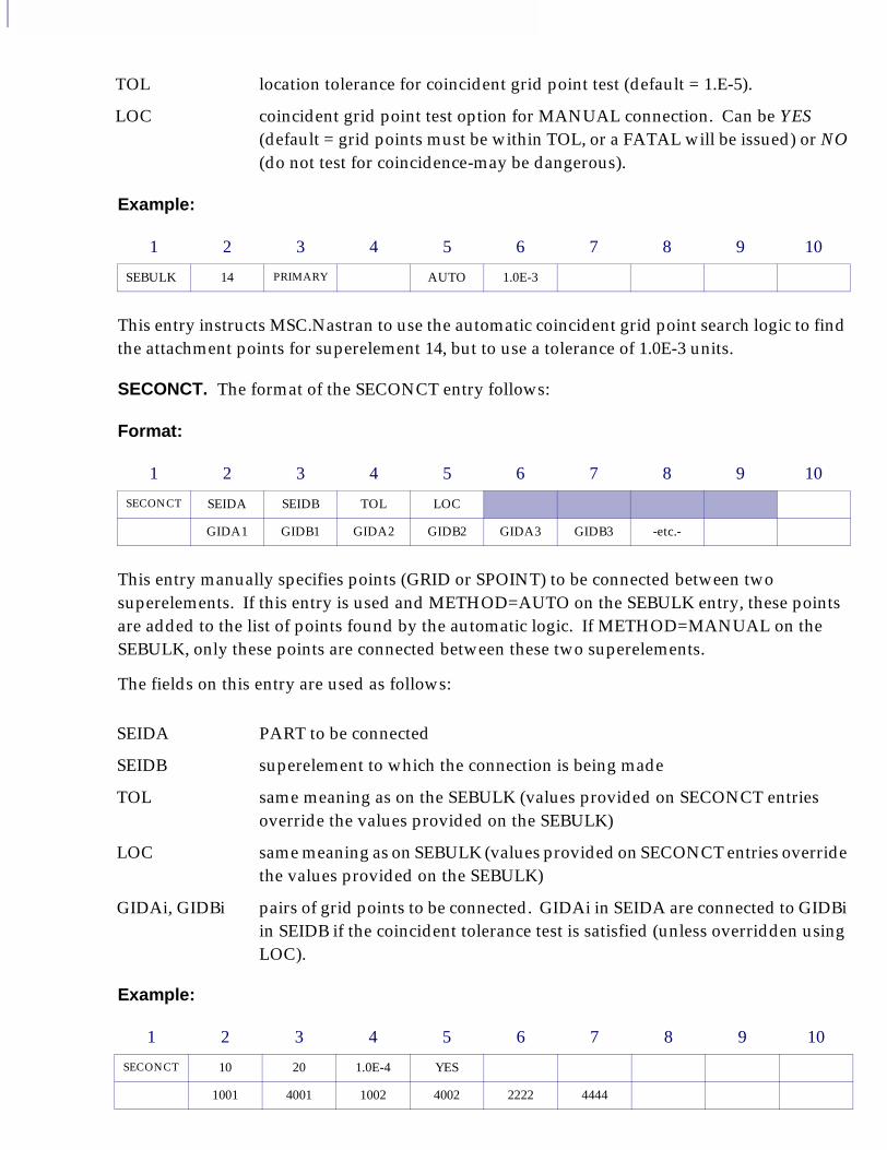
SECONCT. The format of the SECONCT entry follows:
Format:
This entry manually specifies points (GRID or SPOINT) to be connected between two superelements. If this entry is used and METHOD=AUTO on the SEBULK entry, these points are added to the list of points found by the automatic logic. If METHOD=MANUAL on the SEBULK, only these points are connected between these two superelements.
The fields on this entry are used as follows:
Example:
TOL location tolerance for coincident grid point test (default = 1.E-5).
LOC coincident grid point test option for MANUAL connection. Can be YES (default = grid points must be within TOL, or a FATAL will be issued) or NO (do not test for coincidence-may be dangerous).
1 2 3 4 5 6 7 8 9 10
SEBULK 14 PRIMARY AUTO 1.0E-3
1 2 3 4 5 6 7 8 9 10
SECONCT SEIDA SEIDB TOL LOC
GIDA1 GIDB1 GIDA2 GIDB2 GIDA3 GIDB3 -etc.-
SEIDA PART to be connected
SEIDB superelement to which the connection is being made
TOL same meaning as on the SEBULK (values provided on SECONCT entries override the values provided on the SEBULK)
LOC same meaning as on SEBULK (values provided on SECONCT entries override the values provided on the SEBULK)
GIDAi, GIDBi pairs of grid points to be connected. GIDAi in SEIDA are connected to GIDBi in SEIDB if the coincident tolerance test is satisfied (unless overridden using LOC).
1 2 3 4 5 6 7 8 9 10
SECONCT 10 20 1.0E-4 YES
1001 4001 1002 4002 2222 4444

3CHAPTER 2How to Define a Superelement
This entry states that when connecting PART 10 to superelement 20, the tolerance for the coincident grid point test will be 1.0E-4 units and the coincident point test will be performed. This entry also states that we wish to connect point 1001 in PART 10 to point 4001 in superelement 20, point 1002 in PART 10 to point 4002 in superelement 20, and point 2222 in PART 10 to point 4444 in superelement 20 (in this context point can apply to sets of either GRID entries or SPOINTs).
SEEXCLD. The format of the SEEXCLD entry follows:
Format:
This entry is used to limit the automatic search logic. While the SEBNDRY limits the search to selected grid points, the SEEXCLD excludes grid points from the search. Any grid points listed on this entry are grid points in SEIDA that the automatic logic cannot connect to grid points in SEIDB.
Description of the fields on this entry:
Example1:
The above entry states that when connecting PART 110 to superelement 10, grid points 45, 678, and 396 in PART 110 are not considered by the automatic logic.
To show another example of the usage of these entries, we will look at the model used earlier in this section. When we are connecting PART 1 to PART 3, grid points 35 and 36 (which have the same number in both PARTs) are used. This connection can be made in several ways: The example used the automatic connection logic, which determines that these grid points are coincident and connects them; or we could connect these PARTs manually, using the SECONCT entry as follows:
1 2 3 4 5 6 7 8 9 10
SEEXCLD SEIDA SEIDB GIDA1 GIDA2 GIDA3 GIDA4 GIDA5 GIDA6
GIDA7 GIDA8 -etc.-
SEIDA PART for which this entry is used in the automatic search routines.
SEIDB PART(s) for which the search logic uses this list when searching for points coincident to the ones in SEIDA, listed here. This field contains either an integer superelement id or the word ALL if the list is used for all superelements, when searching for coincident points for SEIDA.
GIDAi grid points in SEIDA that cannot be connected to SEIDB if there are coincident points in SEIDB.
1 2 3 4 5 6 7 8 9 10
SEEXCLD 110 10 45 678 396

This entry would not replace the automatic search logic, rather it would confirm that we want to make this connection, in addition to any found by the search logic. If a SEBULK entry were included with METHOD set to MANUAL, then this entry would replace the automatic search logic.
One way to simplify the internal search is to tell the program that only grid points 35 and 36 in PART 1 can be connected to any other superelement.
By doing this, the search logic for connections for PART 1 is simplified. Only grid points 35 and 36 in PART 1 can connect to any other superelement in the model.
Once again, the automatic logic makes the desired connection. The reason for these entries (SEBNDRY, SEBULK, SECONCT, SEEXCLD) is to allow you more control over the search logic. By default, the automatic logic connects any coincident grid points. By using these entries, you can change from fully automatic to semi-automatic (SECONCT plus automatic or using the SEBNDRY or SEEXCLD) or manual (METHOD=MANUAL on the SEBULK with a SECONCT). The choice is yours. The logic for the automatic connection is very efficient-in our testing it took only a few seconds to search over 1,000,000 grid points to find all coincident points in a model. Compared to the amount of time that will be spent solving this problem, this amount of time is negligible.
Manually Defining Exterior Points for a PARTWhen defining a PART it is possible to use ASET, BSET, CSET and/or ASET1, BSET1, CSET1 entries to define exterior points. Any point in a PART that is listed on either an ASET or ASET1 entry is automatically made exterior to that PART (whether there is a coincident point in another superelement or not). All six DOFs of that point are made exterior. The fields on these entries that are used to select DOFs are ignored when these entries are used in PARTs. If there is no coincident point in any other PART, internal points are created in the residual structure that are coincident with the selected points, and the matrices for the PART are connected to these points.
Moving and/or Rotating PARTsIf the model of a PART is not in the correct location or orientation, you can move and/or rotate the part with MSC.Nastran before the program tries to connect it to the other components of the model. This moving and rotating is accomplished using the SELOC entry in the Main Bulk Data Section.
1 2 3 4 5 6 7 8 9 10
SECONCT 1 3
35 35 36 36
1 2 3 4 5 6 7 8 9 10
SEBNDRY 1 ALL 35 36

4CHAPTER 2How to Define a Superelement
Format:
This entry instructs MSC.Nastran to move and/or rotate a PART using three non-colinear GRID entries in the PART and three GRID entries or POINTs (defined in the Main Bulk Data Section), which are located where you would like those entries (in the PART) to be.
The fields on this entry are described as follows:
When this entry is encountered, the program relocates the PART so that grid points PA1-PA3 in the PART are coincident with PB1-PB3 in the main bulk data. This repositioning is performed before the coincident grid point search logic is performed, thus connections for the PART are based on the relocated position. When a PART is relocated like this, the basic coordinate system for the PART is translated and rotated to move the PART into the desired position. Output for the PART is relative to the relocated basic system.
If you request MSC.Nastran plots of the model, any PART that has been translated and/or rotated will appear in its final location. I know of no pre- or post-preprocessor that will display the PART in any location other than its original location and orientation. Therefore, we recommend that you use the MSC.Nastran plotter to view your model after using any SELOC entries. Also, deformed plots are available with PARTs in their final locations. There is an option (SENOMOVE) on the PLOT command that can be used to display PARTs in their original location.
This is a good time to discuss the main bulk data basic coordinate system. When you use PARTs to define a model, each PART is defined in a separate section of the bulk data. As a default, MSC.Nastran assumes that the basic coordinate system for all PARTs is identical to that defined in the Main Bulk Data Section. Therefore, we have a term known as the main bulk data basic coordinate system. As long as your model is defined using the main bulk data basic coordinate system, everything works correctly. But what if different engineers use different basic coordinate systems when modeling components? How do you tell MSC.Nastran the basic coordinate system for PART 5 is different than that for PART 3?
This differentiation is the purpose of the SELOC entry. If the basic coordinate system for any PART is different than that used in the Main Bulk Data Section, it is necessary for you to tell the program how to connect that PART to the rest of the model (that is, the PART will be in the wrong location if we assume that its basic coordinate system is identical to that in the main bulk
1 2 3 4 5 6 7 8 9 10
SELOC SEID PA1 PA2 PA3 PB1 PB2 PB3
SEID PART that is being translated and/or rotated.
PA1-PA3 Three GRID entries in the PART that are to be used to move the PART. After moving, these points will be coincident with PB1-PB3.
PB1-PB3 Three points (either GRID or POINT entries) defined in the Main Bulk Data Section that define where the PART should be.
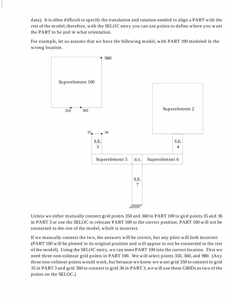
data). It is often difficult to specify the translation and rotation needed to align a PART with the rest of the model; therefore, with the SELOC entry you can use points to define where you want the PART to be and in what orientation.
For example, let us assume that we have the following model, with PART 100 modeled in the wrong location.
Unless we either manually connect grid points 350 and 360 in PART 100 to gird points 35 and 36 in PART 3 or use the SELOC to relocate PART 100 to the correct position, PART 100 will not be connected to the rest of the model, which is incorrect.
If we manually connect the two, the answers will be correct, but any plots will look incorrect (PART 100 will be plotted in its original position and will appear to not be connected to the rest of the model). Using the SELOC entry, we can move PART 100 into the correct location. First we need three non-colinear grid points in PART 100. We will select points 350, 360, and 980. (Any three non-colinear points would work, but because we know we want grid 350 to connect to grid 35 in PART 3 and grid 360 to connect to grid 36 in PART 3, we will use these GRIDs as two of the points on the SELOC.)
Superelement 100
Superelement 2
S.E.3
S.E.4
Superelement 5 Superelement 6
S.E.7
R.S.
35 36
350 360
980
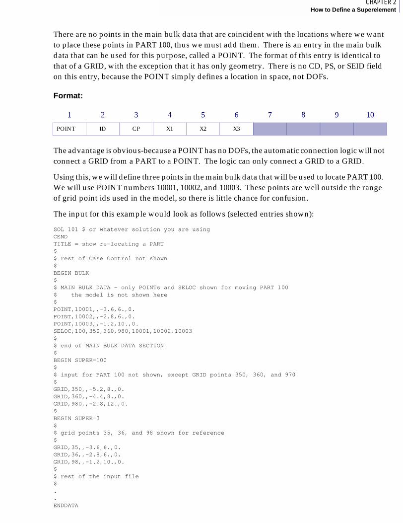
4CHAPTER 2How to Define a Superelement
There are no points in the main bulk data that are coincident with the locations where we want to place these points in PART 100, thus we must add them. There is an entry in the main bulk data that can be used for this purpose, called a POINT. The format of this entry is identical to that of a GRID, with the exception that it has only geometry. There is no CD, PS, or SEID field on this entry, because the POINT simply defines a location in space, not DOFs.
Format:
The advantage is obvious-because a POINT has no DOFs, the automatic connection logic will not connect a GRID from a PART to a POINT. The logic can only connect a GRID to a GRID.
Using this, we will define three points in the main bulk data that will be used to locate PART 100. We will use POINT numbers 10001, 10002, and 10003. These points are well outside the range of grid point ids used in the model, so there is little chance for confusion.
The input for this example would look as follows (selected entries shown):
SOL 101 $ or whatever solution you are usingCENDTITLE = show re-locating a PART$$ rest of Case Control not shown$BEGIN BULK$$ MAIN BULK DATA - only POINTs and SELOC shown for moving PART 100$ the model is not shown here$POINT,10001,,-3.6,6.,0.POINT,10002,,-2.8,6.,0.POINT,10003,,-1.2,10.,0.SELOC,100,350,360,980,10001,10002,10003$$ end of MAIN BULK DATA SECTION$BEGIN SUPER=100$ $ input for PART 100 not shown, except GRID points 350, 360, and 970$GRID,350,,-5.2,8.,0.GRID,360,,-4.4,8.,0.GRID,980,,-2.8,12.,0.$BEGIN SUPER=3$$ grid points 35, 36, and 98 shown for reference$GRID,35,,-3.6,6.,0.GRID,36,,-2.8,6.,0.GRID,98,,-1.2,10.,0.$$ rest of the input file$..ENDDATA
1 2 3 4 5 6 7 8 9 10
POINT ID CP X1 X2 X3
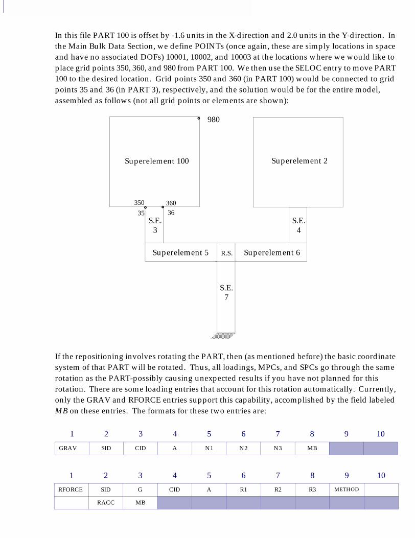
In this file PART 100 is offset by -1.6 units in the X-direction and 2.0 units in the Y-direction. In the Main Bulk Data Section, we define POINTs (once again, these are simply locations in space and have no associated DOFs) 10001, 10002, and 10003 at the locations where we would like to place grid points 350, 360, and 980 from PART 100. We then use the SELOC entry to move PART 100 to the desired location. Grid points 350 and 360 (in PART 100) would be connected to grid points 35 and 36 (in PART 3), respectively, and the solution would be for the entire model, assembled as follows (not all grid points or elements are shown):
If the repositioning involves rotating the PART, then (as mentioned before) the basic coordinate system of that PART will be rotated. Thus, all loadings, MPCs, and SPCs go through the same rotation as the PART-possibly causing unexpected results if you have not planned for this rotation. There are some loading entries that account for this rotation automatically. Currently, only the GRAV and RFORCE entries support this capability, accomplished by the field labeled MB on these entries. The formats for these two entries are:
1 2 3 4 5 6 7 8 9 10
GRAV SID CID A N1 N2 N3 MB
1 2 3 4 5 6 7 8 9 10
RFORCE SID G CID A R1 R2 R3 METHOD
RACC MB
Superelement 100 Superelement 2
S.E.3
S.E.4
Superelement 5 Superelement 6
S.E.7
R.S.
35 36
350 360
980

4CHAPTER 2How to Define a Superelement
The MB field on these two entries tells the program whether the loading is defined using a coordinate system defined in the PART (and therefore rotated with the PART), which is the default, or whether the coordinate system is defined in the Main Bulk Data Section (MB=-1). If the load is defined using a coordinate system from the Main Bulk Data Section, the loading does not rotate with the PART; rather, the loading retains the original orientation based on the selected coordinate system in the Main Bulk Data Section.
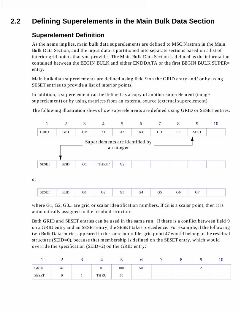
2.2 Defining Superelements in the Main Bulk Data Section
Superelement DefinitionAs the name implies, main bulk data superelements are defined to MSC.Nastran in the Main Bulk Data Section, and the input data is partitioned into separate sections based on a list of interior grid points that you provide. The Main Bulk Data Section is defined as the information contained between the BEGIN BULK and either ENDDATA or the first BEGIN BULK SUPER= entry.
Main bulk data superelements are defined using field 9 on the GRID entry and/or by using SESET entries to provide a list of interior points.
In addition, a superelement can be defined as a copy of another superelement (image superelement) or by using matrices from an external source (external superelement).
The following illustration shows how superelements are defined using GRID or SESET entries.
or
where G1, G2, G3... are grid or scalar identification numbers. If Gi is a scalar point, then it is automatically assigned to the residual structure.
Both GRID and SESET entries can be used in the same run. If there is a conflict between field 9 on a GRID entry and an SESET entry, the SESET takes precedence. For example, if the following two Bulk Data entries appeared in the same input file, grid point 47 would belong to the residual structure (SEID=0), because that membership is defined on the SESET entry, which would override the specification (SEID=2) on the GRID entry:
1 2 3 4 5 6 7 8 9 10
GRID GID CP X1 X2 X3 CD PS SEID
SESET SEID G1 "THRU" G2
SESET SEID G1 G2 G3 G4 G5 G6 G7
1 2 3 4 5 6 7 8 9 10
GRID 47 0. 100. 50. 2
SESET 0 1 THRU 50
Superelements are identified by an integer

4CHAPTER 2How to Define a Superelement
There is no limit on the number of SESET entries that can be used to define a superelement, and with the THRU option on the SESET entry, you can have open sets. That is, not all grid points in the range specified need to exist. If a nonexistent grid point is referenced by an SESET entry, that part of the entry is ignored.
Any grid points defined in the main bulk data that are not assigned to a superelement, using either a SESET or GRID entry, automatically belong to the residual structure (SEID 0). If SPOINTs or EPOINTs exist in the input stream, they automatically belong to the residual structure and can not be interior to a superelement.
Interior Versus Exterior PointsAny grid point assigned to a superelement by the user is interior to that superelement. Exterior grid points are defined by the program based on processing order. If a grid point is connected to a superelement but is interior to a downstream superelement (one which is processed later), that grid point is exterior to the upstream superelement. Processing order can be defined by either the user (see “Multilevel Superelement Analysis” in Chapter 7) or the program. Until “Multilevel Superelement Analysis” in Chapter 7, we will limit the discussion to what is known as a single-level processing tree, where all exterior points of the superelements are interior to the residual structure.
Bulk Data PartitioningThe Main Bulk Data Section is partitioned based on user input (this is done internally using tables, but it is easier to visualize in terms of the bulk data). Once the program detects either SESET entries or entries in field 9 of a GRID entry, the input is partitioned. A separate set of bulk data is created for each superelement, based on input definitions provided by the user.
The partitioning process for the main bulk data is described as follows. First the processing order is defined for the model. Once the processing order is defined, bulk data is partitioned for each superelement in the same order as the processing occurs. All grid points (interior) assigned to the superelement by SESET and GRID entries are removed from the main bulk data and placed in a separate area for the superelement. The next step is to remove all elements (interior) connected to the interior grid points of the superelement. Once this is done, copies are made of all exterior points (grid points that are not interior, but are connected by the elements contained within the superelement). Any loading entries specific to the interior grid points and/or interior elements are removed from the bulk data. Any information removed from the bulk data for a superelement is not available for use in any other superelement. Copies are made of common data-for example, property entries and GRAV entries. Common information is not removed, rather this information is copied so that it will be available for the other superelements.
Once all information for the first superelement has been separated, the process is repeated for the next superelement. After the bulk data has been separated for all superelements, any remaining data belongs to the residual structure.
Once the main bulk data has been partitioned, each superelement is processed using its own unique bulk data. If there are entries that need information from more than one superelement for processing (for example, PLOAD4 entries with a THRU range including elements from
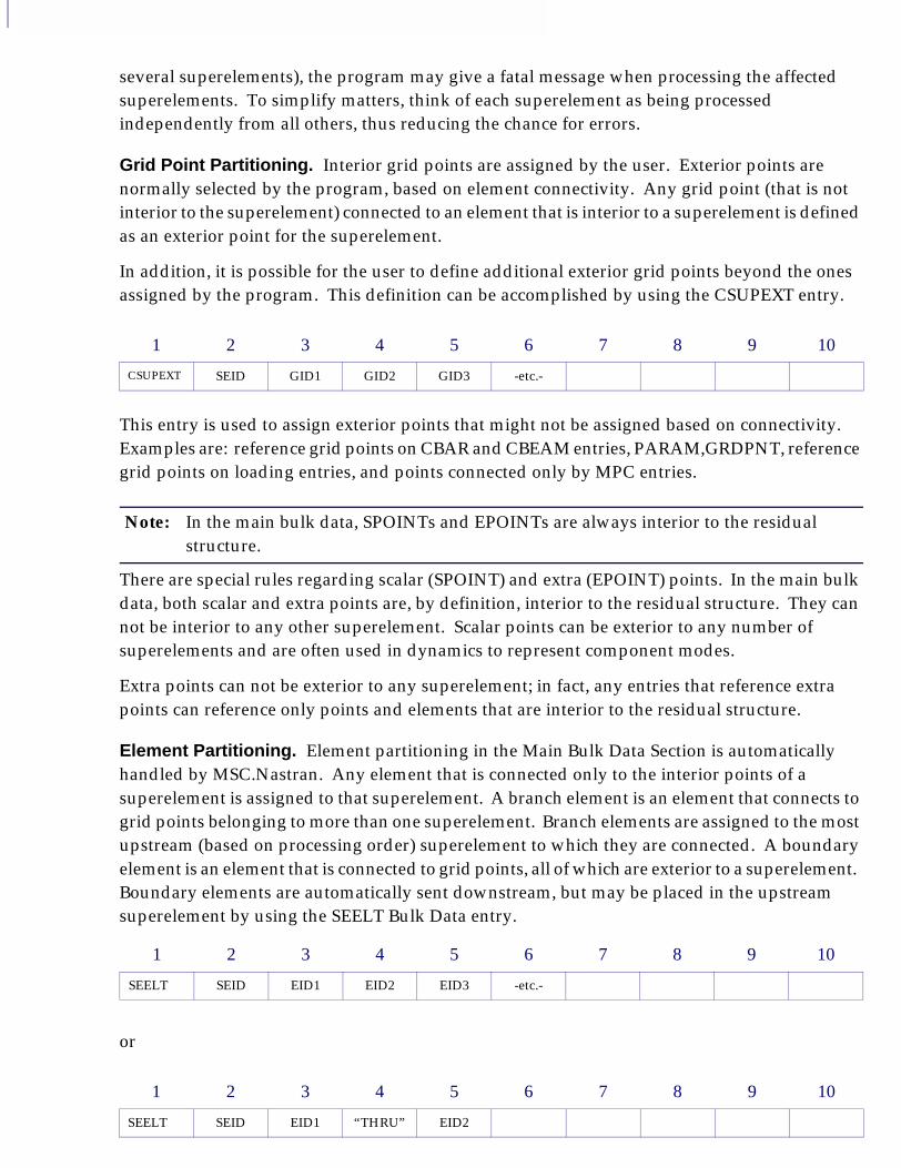
several superelements), the program may give a fatal message when processing the affected superelements. To simplify matters, think of each superelement as being processed independently from all others, thus reducing the chance for errors.
Grid Point Partitioning. Interior grid points are assigned by the user. Exterior points are normally selected by the program, based on element connectivity. Any grid point (that is not interior to the superelement) connected to an element that is interior to a superelement is defined as an exterior point for the superelement.
In addition, it is possible for the user to define additional exterior grid points beyond the ones assigned by the program. This definition can be accomplished by using the CSUPEXT entry.
This entry is used to assign exterior points that might not be assigned based on connectivity. Examples are: reference grid points on CBAR and CBEAM entries, PARAM,GRDPNT, reference grid points on loading entries, and points connected only by MPC entries.
There are special rules regarding scalar (SPOINT) and extra (EPOINT) points. In the main bulk data, both scalar and extra points are, by definition, interior to the residual structure. They can not be interior to any other superelement. Scalar points can be exterior to any number of superelements and are often used in dynamics to represent component modes.
Extra points can not be exterior to any superelement; in fact, any entries that reference extra points can reference only points and elements that are interior to the residual structure.
Element Partitioning. Element partitioning in the Main Bulk Data Section is automatically handled by MSC.Nastran. Any element that is connected only to the interior points of a superelement is assigned to that superelement. A branch element is an element that connects to grid points belonging to more than one superelement. Branch elements are assigned to the most upstream (based on processing order) superelement to which they are connected. A boundary element is an element that is connected to grid points, all of which are exterior to a superelement. Boundary elements are automatically sent downstream, but may be placed in the upstream superelement by using the SEELT Bulk Data entry.
or
1 2 3 4 5 6 7 8 9 10
CSUPEXT SEID GID1 GID2 GID3 -etc.-
Note: In the main bulk data, SPOINTs and EPOINTs are always interior to the residual structure.
1 2 3 4 5 6 7 8 9 10
SEELT SEID EID1 EID2 EID3 -etc.-
1 2 3 4 5 6 7 8 9 10
SEELT SEID EID1 “THRU” EID2
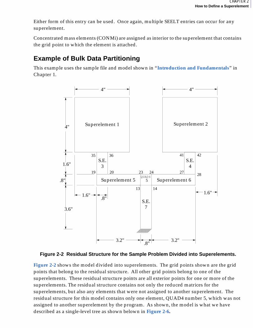
4CHAPTER 2How to Define a Superelement
Either form of this entry can be used. Once again, multiple SEELT entries can occur for any superelement.
Concentrated mass elements (CONMi) are assigned as interior to the superelement that contains the grid point to which the element is attached.
Example of Bulk Data PartitioningThis example uses the sample file and model shown in “Introduction and Fundamentals” in Chapter 1.
Figure 2-2 Residual Structure for the Sample Problem Divided into Superelements.
Figure 2-2 shows the model divided into superelements. The grid points shown are the grid points that belong to the residual structure. All other grid points belong to one of the superelements. These residual structure points are all exterior points for one or more of the superelements. The residual structure contains not only the reduced matrices for the superelements, but also any elements that were not assigned to another superelement. The residual structure for this model contains only one element, QUAD4 number 5, which was not assigned to another superelement by the program. As shown, the model is what we have described as a single-level tree as shown belown in Figure 2-6.
QUAD4
4" 4"
4"
1.6"
1.6" 1.6".8"
.8"
.8"3.2" 3.2"
3.6"
35 36 41 42
13 14
19 20 23 24 2728
5
Superelement 1 Superelement 2
S.E.3
S.E.4
Superelement 5 Superelement 6
S.E.7
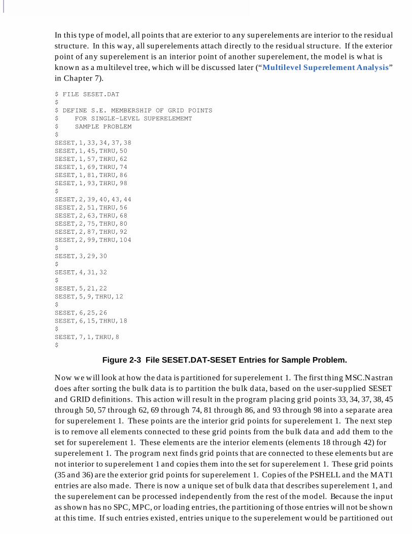
In this type of model, all points that are exterior to any superelements are interior to the residual structure. In this way, all superelements attach directly to the residual structure. If the exterior point of any superelement is an interior point of another superelement, the model is what is known as a multilevel tree, which will be discussed later (“Multilevel Superelement Analysis” in Chapter 7).
$ FILE SESET.DAT$$ DEFINE S.E. MEMBERSHIP OF GRID POINTS $ FOR SINGLE-LEVEL SUPERELEMEMT$ SAMPLE PROBLEM $SESET,1,33,34,37,38SESET,1,45,THRU,50SESET,1,57,THRU,62SESET,1,69,THRU,74SESET,1,81,THRU,86SESET,1,93,THRU,98$SESET,2,39,40,43,44SESET,2,51,THRU,56SESET,2,63,THRU,68SESET,2,75,THRU,80SESET,2,87,THRU,92SESET,2,99,THRU,104$SESET,3,29,30$SESET,4,31,32$SESET,5,21,22SESET,5,9,THRU,12$SESET,6,25,26SESET,6,15,THRU,18$SESET,7,1,THRU,8$
Figure 2-3 File SESET.DAT-SESET Entries for Sample Problem.
Now we will look at how the data is partitioned for superelement 1. The first thing MSC.Nastran does after sorting the bulk data is to partition the bulk data, based on the user-supplied SESET and GRID definitions. This action will result in the program placing grid points 33, 34, 37, 38, 45 through 50, 57 through 62, 69 through 74, 81 through 86, and 93 through 98 into a separate area for superelement 1. These points are the interior grid points for superelement 1. The next step is to remove all elements connected to these grid points from the bulk data and add them to the set for superelement 1. These elements are the interior elements (elements 18 through 42) for superelement 1. The program next finds grid points that are connected to these elements but are not interior to superelement 1 and copies them into the set for superelement 1. These grid points (35 and 36) are the exterior grid points for superelement 1. Copies of the PSHELL and the MAT1 entries are also made. There is now a unique set of bulk data that describes superelement 1, and the superelement can be processed independently from the rest of the model. Because the input as shown has no SPC, MPC, or loading entries, the partitioning of those entries will not be shown at this time. If such entries existed, entries unique to the superelement would be partitioned out

5CHAPTER 2How to Define a Superelement
and placed in the set for superelement 1, and information that was shared would be copied into the information for superelement 1 (see “Loads, Constraints, and Case Control in Static Analysis” in Chapter 4 for a description of this process).
Figure 2-4 Superelement 1.
The partitioned model for superelement 1 is shown in Figure 2-4. The exterior points are marked with x. During the processing, MSC.Nastran replaces this finite element model of superelement 1 with a set of reduced matrices that represent the mass, stiffness, and damping properties of superelement 1, as seen by the adjoining structure. In later chapters this process will be shown in a manner similar to that shown in Figure 2-5.
Elements 18 through 42 are interior to superelement 1. Elements 19, 20, and 21 are known as branch elements, because they are connected to grid points belonging to both superelement 1 and the residual structure. As mentioned before, these elements are assigned to the upstream superelement, or superelement 1.
If a CBAR element were connected to grid points 35 and 36, it would be a boundary element (i.e., connected to grid points that were both exterior to superelement 1). By default, the CBAR would belong to the residual structure. However, the CBAR could be moved into superelement 1 by using an SEELT entry. For example, if the following CBAR element connectivity existed,
then a FATAL error would occur (since GRID 71 is used for orientation)unless the CBAR was assigned to superelement 1, using the following SEELT entry.
The reason for this error is as follows: MSC.Nastran looks only at the element connectivity when assigning elements to superelements. CBAR 1000 connects to grid points 35 and 36 and finds they both belong to the residual structure. The CBAR is then assigned interior to the residual structure. Because of this, without the SEELT entry a FATAL message occurs when processing
1 2 3 4 5 6 7 8 9 10
CBAR 1000 1 35 36 71
1 2 3 4 5 6 7 8 9 10
SEELT 1 1000
93 94 95 96 97 98
38 39 40 41 42
33 34 35 36 37
28 29 30 31 32
23 24 25 26 27
18 19 20 21 22
81
69
57
45
33
86
74
62
50
3834 35 36 37
x x
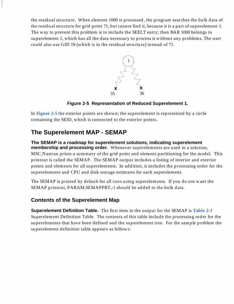
the residual structure. When element 1000 is processed, the program searches the bulk data of the residual structure for grid point 71, but cannot find it, because it is a part of superelement 1. The way to prevent this problem is to include the SEELT entry; then BAR 1000 belongs to superelement 1, which has all the data necessary to process it without any problems. The user could also use GID 19 (which is in the residual structure) instead of 71.
Figure 2-5 Representation of Reduced Superelement 1.
In Figure 2-5 the exterior points are shown; the superelement is represented by a circle containing the SEID, which is connected to the exterior points.
The Superelement MAP - SEMAP
The SEMAP is a roadmap for superelement solutions, indicating superelement membership and processing order. Whenever superelements are used in a solution, MSC.Nastran prints a summary of the grid point and element partitioning for the model. This printout is called the SEMAP. The SEMAP output includes a listing of interior and exterior points and elements for all superelements. In addition, it includes the processing order for the superelements and CPU and disk storage estimates for each superelement.
The SEMAP is printed by default for all runs using superelements. If you do not want the SEMAP printout, PARAM,SEMAPPRT,-1 should be added to the bulk data.
Contents of the Superelement Map
Superelement Definition Table. The first item in the output for the SEMAP is Table 2-1 Superelement Definition Table. The contents of this table include the processing order for the superelements that have been defined and the superelement tree. For the sample problem the superelement definition table appears as follows:
1
x x35 36
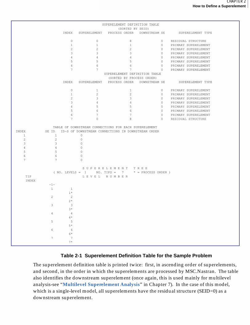
5CHAPTER 2How to Define a Superelement
Table 2-1 Superelement Definition Table for the Sample Problem
The superelement definition table is printed twice: first, in ascending order of superelements, and second, in the order in which the superelements are processed by MSC.Nastran. The table also identifies the downstream superelement (once again, this is used mainly for multilevel analysis-see “Multilevel Superelement Analysis” in Chapter 7). In the case of this model, which is a single-level model, all superelements have the residual structure (SEID=0) as a downstream superelement.
SUPERELEMENT DEFINITION TABLE (SORTED BY SEID) INDEX SUPERELEMENT PROCESS ORDER DOWNSTREAM SE SUPERELEMENT TYPE 0 0 8 0 RESIDUAL STRUCTURE 1 1 1 0 PRIMARY SUPERELEMENT 2 2 2 0 PRIMARY SUPERELEMENT 3 3 3 0 PRIMARY SUPERELEMENT 4 4 4 0 PRIMARY SUPERELEMENT 5 5 5 0 PRIMARY SUPERELEMENT 6 6 6 0 PRIMARY SUPERELEMENT 7 7 7 0 PRIMARY SUPERELEMENT SUPERELEMENT DEFINITION TABLE (SORTED BY PROCESS ORDER) INDEX SUPERELEMENT PROCESS ORDER DOWNSTREAM SE SUPERELEMENT TYPE
0 1 1 0 PRIMARY SUPERELEMENT 1 2 2 0 PRIMARY SUPERELEMENT 2 3 3 0 PRIMARY SUPERELEMENT 3 4 4 0 PRIMARY SUPERELEMENT 4 5 5 0 PRIMARY SUPERELEMENT 5 6 6 0 PRIMARY SUPERELEMENT 6 7 7 0 PRIMARY SUPERELEMENT 7 0 8 0 RESIDUAL STRUCTURE
TABLE OF DOWNSTREAM CONNECTIONS FOR EACH SUPERELEMENT INDEX SE ID ID-S OF DOWNSTREAM CONNECTIONS IN DOWNSTREAM ORDER 1 1 0 2 2 0 3 3 0 4 4 0 5 5 0 6 6 0 7 7 0 S U P E R E L E M E N T T R E E ( NO. LEVELS = 1 NO. TIPS = 7 * = PROCESS ORDER ) TIP L E V E L N U M B E R INDEX -1- 1 1 1* 2 2 2* 3 3 3* 4 4 4* 5 5 5* 6 6 6* 7 7 7*
The farthest right-hand column has a description of the type of each superelement. In this example all superelements are primary superelements, meaning that each superelement has its own unique bulk data. The other types of superelements are: identical and mirror images, and external superelements.
The next set of information is the table of downstream connections for each superelement. This table is useful in identifying multilevel configurations. For a single-level tree, as shown, the table only verifies what we already know.
The next part is the superelement tree. In printed form a representation of the processing order resembles a tree. For a single-level tree the processing order only repeats what we already know; however, for a multilevel tree the order is important not only for initial processing, but for restarts, in that it shows the path to follow when changes are made. Think of the processing order as a tree, where the processing must flow down the tree and data recovery is performed by climbing the tree. Figure 2-6 helps explain the printout and shows a graphical representation of the tree.
The printed form shows the processing tree sideways. In the printed form, each superelement appears as its SEID. Below each superelement ID appears the processing order for that superelement. Once again, because this is a simple problem, the processing order matches the SEID, which is generally not the case in more complicated problems.
Figure 2-6 Graphical Superelement Tree.
Figure 2-6 shows the superelement tree in a more convenient form. In this form we can see that each superelement has its own branch and, therefore, its own path. Each superelement attaches only to the residual structure (SEID=0) and can be processed independently from all other superelements. When a model is defined in this manner, it is known as a single-level tree. For processing, the order goes down the tree, or directly from each superelement to the residual, indicating that all superelements must be processed before the residual structure (assembly) can be solved. Once the problem is solved, data recovery progresses up the tree, meaning that once the residual structure solution is available, data recovery can be preformed for any of the superelements in this model in any order. If we had a multilevel tree, there would be paths that must be followed for obtaining desired superelement results (see “Multilevel Superelement Analysis” in Chapter 7).
1 2 3 4 5 6 7
0
MSC.Nastran Superelements User’s Guide
CHAPTER
3 Single-Level Superelement Analysis
■ Introduction
■ Simple Input for Single-Level Analysis

3.1 IntroductionWe have defined single-level analysis as one in which all superelements connect to the residual structure only. Single-level superelement analysis occurs when the exterior points of all superelements in the model are interior to the residual structure. In this case each superelement can be processed independently from all other superelements.
This means that any boundary points where two or more superelements meet belong to the residual structure. Single-level analysis is the simplest form of superelement analysis and is recommended for the beginning superelement user. Partitioning the model into superelements for a single-level analysis requires the least effort from the user, and processing control (if desired) is simple.
It should be noted that if PARTs are used, the model is automatically a single-level model unless either DTI,SETREE or SETREE entries exists in the Main Bulk Data Section. If the model is defined as a Main Bulk Data Section only model, care must be taken to verify that all exterior points belong to the residual structure; otherwise, a multilevel processing tree (“Multilevel Superelement Analysis” in Chapter 7) is created automatically.
In addition to single level being recommended for the beginning superelement user, single-level analysis is recommended for use in the analysis of structures that are expected to change often and in many areas. For this case, where there is no knowledge of areas that will not be changing, a single-level model is almost always the most efficient. Consequently, when a change occurs only the affected superelement and the residual structure need to be processed again. Therefore, restarts for model change can be very efficient. In fact, this is one of the biggest advantages of using superelements.
A good example is a spacecraft upper stage booster model that the author used in support of a modal test. The model consisted of approximately 30,000 DOFs. To provide real time support to the test, modal runs incorporating changes in the model were necessary for evaluating how a change to the model might improve the match between test and analysis results. Initially, the entire model was being run for modes; this run took 29 CPU hours (in 1985, it would run much faster on a current version of MSC.Nastran). On a heavily loaded computer, this run required about five days-obviously not real time turnaround. To improve the turnaround time, the model was divided into superelements based on an understanding of the structure and the areas expected to change. For this model any areas that were expected to change were placed in the residual structure, and the rest of the model was placed in upstream superelements. Once this was done, an initial superelement run was performed. The initial run did not save any time (as expected). However, restart runs to evaluate the effects of a model change took only 1 CPU hour to run, including data recovery; a 29:1 performance improvement. Also, two runs could be processed in one day, compared to one run in a week, without superelements.
5CHAPTER 3Single-Level Superelement Analysis
3.2 Simple Input for Single-Level Analysis
This chapter contains the minimum information required to convert an existing model to superelements. The simplest approach you can use for performing a superelement analysis is a single-level processing tree. In a single-level analysis all points that are exterior to any superelement are interior to the residual structure. More simply, the points that are used to connect the superelements (exterior points) must belong to the residual structure. If any exterior point of any superelement belongs to another superelement, then the model is a multilevel model; this type of analysis is described later.
You are not required to use single- or multilevel analysis for any problem. You will discover, as you become a more advanced user, that some models lend themselves to a single-level analysis and others lend themselves to a multilevel analysis. In statics the two approaches provide identical answers. In dynamic analysis you may obtain different answers with a single-level solution than you would using a multilevel solution. This is discussed in the chapter on superelements in dynamic analysis.
Single-Level Analysis Using Main Bulk Data SuperelementsBecause main bulk data superelements are defined by you, if you wish to use a single-level processing tree, you must be sure that all exterior points belong to the residual structure. If any exterior points belong to another superelement, MSC.Nastran automatically creates a multilevel tree (if the model contains no PARTs).
For simplicity we will assume that an input file exists that can be used to perform a static solution on the model without superelements. That is, we will begin with an input file ready to run in a non-superelement static solution.
The input required to change from a conventional static analysis to a single-level superelement analysis is minimal. The steps are as follows:
1. Define the superelements (to make a single-level model, make sure that the boundary points belong to the residual structure).
2. Run using SOL 101.
These steps are the only requirement for changing a model from conventional analysis into single-level superelement analysis (the format of the super case control command is covered in “Loads, Constraints, and Case Control in Static Analysis” in Chapter 4). If you only want to switch your model into a superelement model and run, you now have enough information.
However, a few limitations do exist: If you are using multiple boundary conditions, they must be contained in the residual structure (the ability to solve with multiple residual structure boundary conditions was introduced in Version 68), and if you are using inertia relief, there is an additional entry (PARAM,INREL,-1), which is described in “Inertia Relief Analysis Using Superelements” in Chapter 5. For most static analysis input files, these requirements are all you need to convert from conventional to superelement analysis. The rest of this User’s Guide demonstrates advanced features and how to use superelements in dynamic analysis.
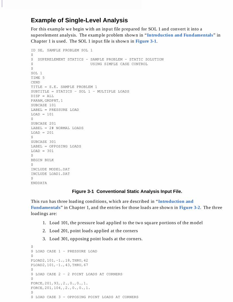
Example of Single-Level AnalysisFor this example we begin with an input file prepared for SOL 1 and convert it into a superelement analysis. The example problem shown in “Introduction and Fundamentals” in Chapter 1 is used. The SOL 1 input file is shown in Figure 3-1.
ID SE, SAMPLE PROBLEM SOL 1$$ SUPERELEMENT STATICS - SAMPLE PROBLEM - STATIC SOLUTION$ USING SIMPLE CASE CONTROL$ SOL 1TIME 5CENDTITLE = S.E. SAMPLE PROBLEM 1 SUBTITLE = STATICS - SOL 1 - MULTIPLE LOADSDISP = ALLPARAM,GRDPNT,1SUBCASE 101LABEL = PRESSURE LOADLOAD = 101$SUBCASE 201LABEL = 2# NORMAL LOADSLOAD = 201$SUBCASE 301LABEL = OPPOSING LOADSLOAD = 301$BEGIN BULK$INCLUDE MODEL.DATINCLUDE LOAD1.DAT$ENDDATA
Figure 3-1 Conventional Static Analysis Input File.
This run has three loading conditions, which are described in “Introduction and Fundamentals” in Chapter 1, and the entries for those loads are shown in Figure 3-2. The three loadings are:
1. Load 101, the pressure load applied to the two square portions of the model
2. Load 201, point loads applied at the corners
3. Load 301, opposing point loads at the corners.
$$ LOAD CASE 1 - PRESSURE LOAD$PLOAD2,101,-1.,18,THRU,42PLOAD2,101,-1.,43,THRU,67$$ LOAD CASE 2 - 2 POINT LOADS AT CORNERS$FORCE,201,93,,2.,0.,0.,1.FORCE,201,104,,2.,0.,0.,1.$$ LOAD CASE 3 - OPPOSING POINT LOADS AT CORNERS

5CHAPTER 3Single-Level Superelement Analysis
$FORCE,301,93,,2.,0.,0.,1.FORCE,301,104,,2.,0.,0.,-1.$
Figure 3-2 File Load1.dat.
Now we will change this file into a superelement model. First we add the SESET entries (by including the file seset.dat from “How to Define a Superelement” in Chapter 2). Once this is done, we change to SOL 101. The file shown in Figure 3-3 includes these changes (shown in bold). This file is ready to run and gives the same answers as those originally obtained in SOL 1.
ID SE, SAMPLE PROBLEM SOL 101$$ SUPERELEMENT STATICS - SAMPLE PROBLEM - STATIC SOLUTION$ USING SIMPLE CASE CONTROL$ SOL 101 $ SUPERELEMENT STATICS - SINGLE LEVEL TREE$TIME 15CENDTITLE = S.E. SAMPLE PROBLEM 1 SUBTITLE = S.E. STATICS - RUN 1 - MULTIPLE LOADSDISP = ALL$$SUBCASE 101LABEL = PRESSURE LOADLOAD = 101$SUBCASE 201LABEL = 2# NORMAL LOADSLOAD = 201$SUBCASE 301LABEL = OPPOSING LOADSLOAD = 301$$BEGIN BULKPARAM,POST,0$INCLUDE SESET.DAT$INCLUDE MODEL.DATINCLUDE LOAD1.DAT$ENDDATA
Figure 3-3 File SE1S101.DAT.
Quick ReviewEnough information has now been given to allow a single-level superelement static run to be performed using main bulk data superelements. Review the most important items listed below.
• Define the superelements to MSC.Nastran using field 9 on the GRID entry and/or SESET entries.

• MSC.Nastran automatically partitions the information in the Main Bulk Data Section for you.
• In case control add SUPER = ALL above the first SUBCASE (optional-see the next chapter).
• Use SOL 101 for statics.
• The information given in this chapter is the minimum you need to begin using single-level superelement analysis (for proficiency in static analysis, “Loads, Constraints, and Case Control in Static Analysis” in Chapter 4 through “Multiple Loadings in Static Analysis” in Chapter 6 should also be read).
Single-Level Analysis When PARTs Are PresentWhen partitioned bulk data is used (PARTs), MSC.Nastran automatically forces a single-level processing tree. As mentioned in the previous chapter, the program finds all grid points that are coincident between each PART and any other PARTs and/or main bulk data superelements, then (if the grid points are not already in the residual structure) creates internal copies of these points and places those copies in the residual structure. No special effort is required to run a single-level analysis if PARTs are present in the model. However, if you wish to perform a multilevel analysis and PARTs are present, you must manually instruct the program to perform the multilevel solution (see “Multilevel Superelement Analysis” in Chapter 7).
MSC.Nastran Superelements User’s Guide
CHAPTER
4 Loads, Constraints, and Case Control in Static Analysis
■ Introduction
■ Loads in Static Analysis
■ Boundary Conditions
■ Case Control in Superelement Analysis

4.1 IntroductionA very simple first approach to using superelements in static analysis was presented in “Introduction and Fundamentals” in Chapter 1. Now we will go into more detail on how individual items work. For example, the SUPER = ALL command in “Single-Level Superelement Analysis” in Chapter 3 is the simplest form of the SUPER command, yet it has many additional features. Thus, “Single-Level Superelement Analysis” in Chapter 3 was the appetizer and now we are prepared for the main course.
In this chapter we will discuss how loadings and constraints are partitioned when superelements are used and how they are applied in static analysis using Case Control commands.
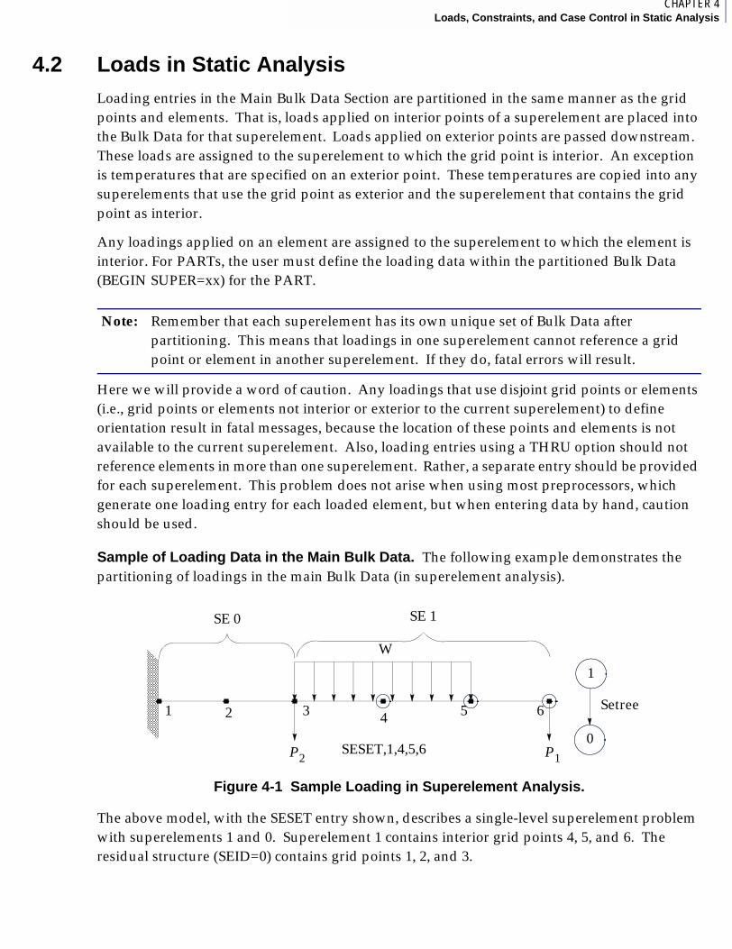
6CHAPTER 4Loads, Constraints, and Case Control in Static Analysis
4.2 Loads in Static AnalysisLoading entries in the Main Bulk Data Section are partitioned in the same manner as the grid points and elements. That is, loads applied on interior points of a superelement are placed into the Bulk Data for that superelement. Loads applied on exterior points are passed downstream. These loads are assigned to the superelement to which the grid point is interior. An exception is temperatures that are specified on an exterior point. These temperatures are copied into any superelements that use the grid point as exterior and the superelement that contains the grid point as interior.
Any loadings applied on an element are assigned to the superelement to which the element is interior. For PARTs, the user must define the loading data within the partitioned Bulk Data (BEGIN SUPER=xx) for the PART.
Here we will provide a word of caution. Any loadings that use disjoint grid points or elements (i.e., grid points or elements not interior or exterior to the current superelement) to define orientation result in fatal messages, because the location of these points and elements is not available to the current superelement. Also, loading entries using a THRU option should not reference elements in more than one superelement. Rather, a separate entry should be provided for each superelement. This problem does not arise when using most preprocessors, which generate one loading entry for each loaded element, but when entering data by hand, caution should be used.
Sample of Loading Data in the Main Bulk Data. The following example demonstrates the partitioning of loadings in the main Bulk Data (in superelement analysis).
Figure 4-1 Sample Loading in Superelement Analysis.
The above model, with the SESET entry shown, describes a single-level superelement problem with superelements 1 and 0. Superelement 1 contains interior grid points 4, 5, and 6. The residual structure (SEID=0) contains grid points 1, 2, and 3.
Note: Remember that each superelement has its own unique set of Bulk Data after partitioning. This means that loadings in one superelement cannot reference a grid point or element in another superelement. If they do, fatal errors will result.
SE 0 SE 1
W
1 2 3 4 5 6
1
0SESET,1,4,5,6P2 P1
Setree

The Bulk Data entries for the applied loadings are partitioned as follows:
Force P1 is applied on grid point 6, which is interior to superelement 1, thus force P1 is partitioned into the Bulk Data for superelement 1.
Force P2 is applied on grid point 3, which is interior to the residual structure, thus force P2 is assigned to the residual structure Bulk Data.
pload W is applied on elements that belong interior to superelement 1; therefore, pload W is partitioned into the Bulk Data for superelement 1.
Bulk data partitioning merely partitions the Bulk Data by superelement--it does not actually apply the loadings. The loadings are applied in the Case Control Section.
Thermal Loadings in Superelement Analysis
Main Bulk Data Thermal Loads. Temperatures described by grid points in the main Bulk Data (TEMP, TEMPD) are partitioned along with the grid points, with the following exception: Any temperatures defined at an exterior point are copied into both the superelement for which the grid point is exterior and the superelement for which the grid point is interior.
Temperatures defined by elements (TEMPPi and TEMPRB) are partitioned in the same manner as the elements.
Partitioned Bulk Data Thermal Loads. Once again, all temperature related loading information for PARTs must be in the partitioned Bulk Data (BEGIN SUPER=xx) for the PART.
Note: The process just described is the partitioning of the Bulk Data for the applied loadings. The application of the loadings is actually controlled by the Case Control and is described later in this chapter.
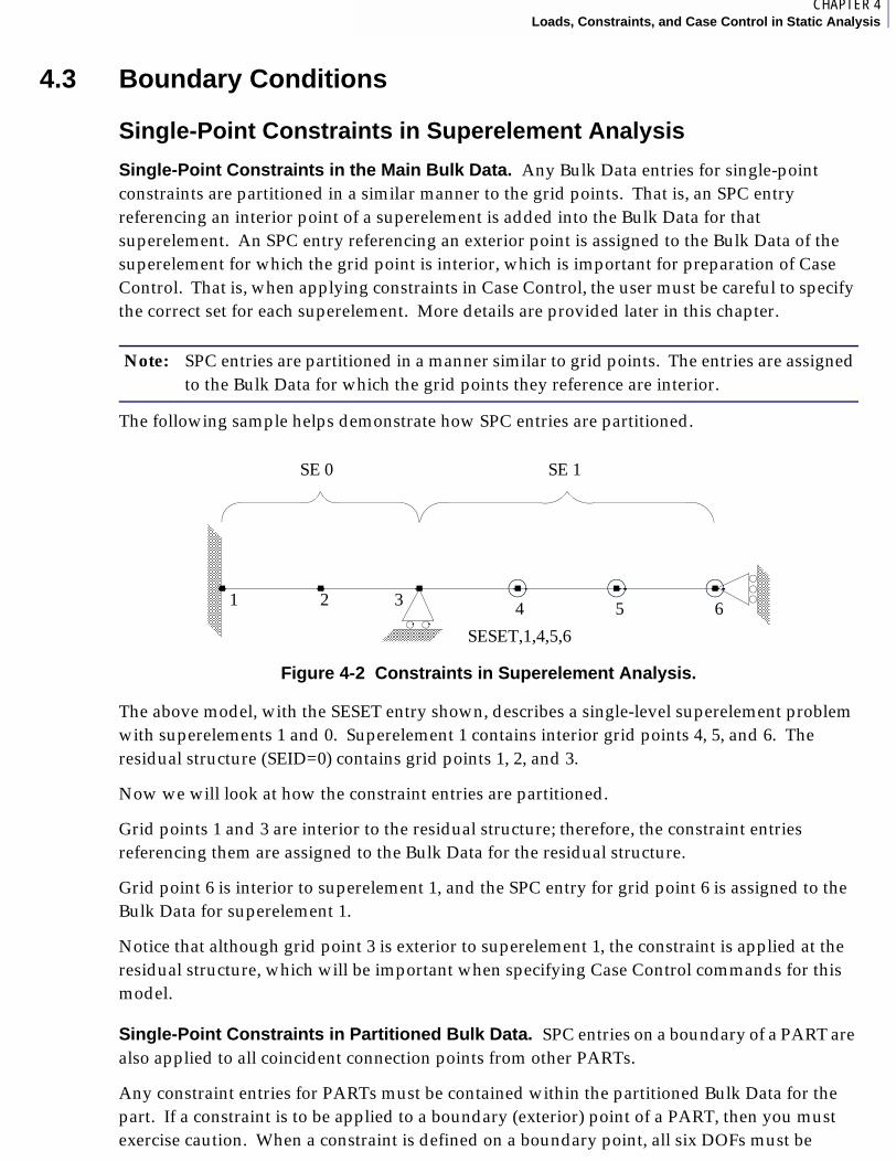
6CHAPTER 4Loads, Constraints, and Case Control in Static Analysis
4.3 Boundary Conditions
Single-Point Constraints in Superelement Analysis
Single-Point Constraints in the Main Bulk Data. Any Bulk Data entries for single-point constraints are partitioned in a similar manner to the grid points. That is, an SPC entry referencing an interior point of a superelement is added into the Bulk Data for that superelement. An SPC entry referencing an exterior point is assigned to the Bulk Data of the superelement for which the grid point is interior, which is important for preparation of Case Control. That is, when applying constraints in Case Control, the user must be careful to specify the correct set for each superelement. More details are provided later in this chapter.
The following sample helps demonstrate how SPC entries are partitioned.
Figure 4-2 Constraints in Superelement Analysis.
The above model, with the SESET entry shown, describes a single-level superelement problem with superelements 1 and 0. Superelement 1 contains interior grid points 4, 5, and 6. The residual structure (SEID=0) contains grid points 1, 2, and 3.
Now we will look at how the constraint entries are partitioned.
Grid points 1 and 3 are interior to the residual structure; therefore, the constraint entries referencing them are assigned to the Bulk Data for the residual structure.
Grid point 6 is interior to superelement 1, and the SPC entry for grid point 6 is assigned to the Bulk Data for superelement 1.
Notice that although grid point 3 is exterior to superelement 1, the constraint is applied at the residual structure, which will be important when specifying Case Control commands for this model.
Single-Point Constraints in Partitioned Bulk Data. SPC entries on a boundary of a PART are also applied to all coincident connection points from other PARTs.
Any constraint entries for PARTs must be contained within the partitioned Bulk Data for the part. If a constraint is to be applied to a boundary (exterior) point of a PART, then you must exercise caution. When a constraint is defined on a boundary point, all six DOFs must be
Note: SPC entries are partitioned in a manner similar to grid points. The entries are assigned to the Bulk Data for which the grid points they reference are interior.
1 2 3 4 5 6
SE 0 SE 1
SESET,1,4,5,6

constrained on that grid point. Exceptions to this are: 1) if all coincident points use the same displacement coordinate system, then selected dof may be constrained, and 2) any constraints desired may be applied in the ‘downstream’ superelement where the point is an interior point.
Grid Point Singularity Processor (PARAM,AUTOSPC,YES). Because each superelement is processed independently, it is possible to turn AUTOSPC on and off, by superelement. Normally, you want to apply AUTOSPC to the entire model (all superelements), and that is the default in the superelement solutions (exception: the nonlinear solutions). However, the grid point singularity processor can be selectively applied to a model, using superelements, by either placing PARAM,AUTOSPC in the Case Control Section and using different values for each superelement (explained later in this chapter), or by specifying different values in the separate Bulk Data Sections for PARTs.
When the grid point singularity processor (AUTOSPC) is used on superelements, it will look only at the interior points of each superelement. Any points that are exterior to a superelement are defined as belonging to the A-set for that superelement. AUTOSPC will not constrain an A-set DOF. The exterior points of a superelement can have elements connected to them from other superelements; therefore, to constrain these points before we have a chance to attach all elements might overconstrain the structure. AUTOSPC looks at these grid points when processing the downstream superelement that contains them as interior points.
In the example used earlier in this chapter, (Figure 4-1) when processing superelement 1, AUTOSPC could only applied constraints to singularities on grid points 4, 5, and 6. Any singularities on grid point 3 (which is exterior) were not constrained while processing superelement 1. Rather, they were constrained when processing the residual structure (which has grid point 3 interior).
Multipoint Constraints (MPCs) and R-Type Elements
MPCs and R-Type Elements in the Main Bulk Data Section
R-type elements (RBE2, RBE3, RBAR, RSSCON, etc.) in the main Bulk Data are treated as elements; i.e., their connectivity is used to determine the superelement’s Bulk Data in which to put them and can be used to determine exterior points.
MPCs are treated in a similar manner, except they are not used to define superelement exterior points. If we think back to “How to Define a Superelement” in Chapter 2, we will remember that element connectivity is used to determine the exterior points for a superelement. Because MPC sets are called in Case Control and different MPC sets can be used in each SUBCASE, MPC sets are not used in the definition of superelements. MPC entries are partitioned according to the interior points of superelements. An MPC entry is assigned to the highest upstream superelement (based on the processing order) to which it connects.
Note: R-type elements are always included in the analysis. MPC entries are onlly included if the MPC set is called out in the Case Control Section for the superelement.
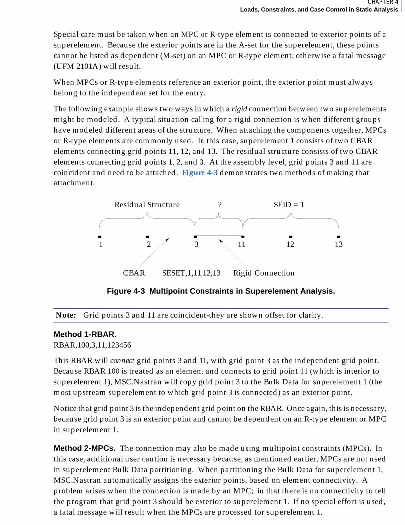
6CHAPTER 4Loads, Constraints, and Case Control in Static Analysis
Special care must be taken when an MPC or R-type element is connected to exterior points of a superelement. Because the exterior points are in the A-set for the superelement, these points cannot be listed as dependent (M-set) on an MPC or R-type element; otherwise a fatal message (UFM 2101A) will result.
When MPCs or R-type elements reference an exterior point, the exterior point must always belong to the independent set for the entry.
The following example shows two ways in which a rigid connection between two superelements might be modeled. A typical situation calling for a rigid connection is when different groups have modeled different areas of the structure. When attaching the components together, MPCs or R-type elements are commonly used. In this case, superelement 1 consists of two CBAR elements connecting grid points 11, 12, and 13. The residual structure consists of two CBAR elements connecting grid points 1, 2, and 3. At the assembly level, grid points 3 and 11 are coincident and need to be attached. Figure 4-3 demonstrates two methods of making that attachment.
Figure 4-3 Multipoint Constraints in Superelement Analysis.
Method 1-RBAR. RBAR,100,3,11,123456
This RBAR will connect grid points 3 and 11, with grid point 3 as the independent grid point. Because RBAR 100 is treated as an element and connects to grid point 11 (which is interior to superelement 1), MSC.Nastran will copy grid point 3 to the Bulk Data for superelement 1 (the most upstream superelement to which grid point 3 is connected) as an exterior point.
Notice that grid point 3 is the independent grid point on the RBAR. Once again, this is necessary, because grid point 3 is an exterior point and cannot be dependent on an R-type element or MPC in superelement 1.
Method 2-MPCs. The connection may also be made using multipoint constraints (MPCs). In this case, additional user caution is necessary because, as mentioned earlier, MPCs are not used in superelement Bulk Data partitioning. When partitioning the Bulk Data for superelement 1, MSC.Nastran automatically assigns the exterior points, based on element connectivity. A problem arises when the connection is made by an MPC; in that there is no connectivity to tell the program that grid point 3 should be exterior to superelement 1. If no special effort is used, a fatal message will result when the MPCs are processed for superelement 1.
Note: Grid points 3 and 11 are coincident-they are shown offset for clarity.
1 2 3 11 12 13
Residual Structure SEID = 1?
CBAR Rigid ConnectionSESET,1,11,12,13

This problem did not appear with the RBAR, because the RBAR is treated as an element for Bulk Data partitioning.
The following MPC entries are used to perform the connection:
MPC,1,11,1,1.,3,1,-1.MPC,1,11,2,1.,3,2,-1.MPC,1,11,3,1.,3,3,-1.MPC,1,11,4,1.,3,4,-1.MPC,1,11,5,1.,3,5,-1.MPC,1,11,6,1.,3,6,-1.
These entries will connect all DOFs of grid point 11 to grid point 3. Note that the coefficients are 1.0, due to the points being coincident.
Grid point 3 is the independent grid point on the MPCs. Once again, an exterior point cannot be dependent on an MPC or R-type element.
Following are two possible methods of assigning grid point 3 as exterior to superelement 1 (to make the connection).
Method 1, CSUPEXT.
CSUPEXT,1,3
This entry will assign grid point 3 as being exterior to superelement 1. Although there is no connection made by elements, this point will now be an exterior point, and the MPCs can be used to perform the connection.
Method 2, PLOTEL. MSC.Nastran treats PLOTELs the same as all other elements when partitioning Bulk Data; therefore, because this element has no stiffness associated with it, the PLOTEL is an ideal element for attaching exterior points to a superelement.
PLOTEL,99,3,11
This element is assigned to superelement 1, because superelement 1 is the highest superelement in the processing tree that connects to this element. A plotel used with MPCs is also a device to symbolize MPCs on structure plots. When assigning exterior points to superelement 1, MSC.Nastran assigns grid point 3 as exterior, because this point is connected to PLOTEL number 99.
MPCs and R-Type Elements in PARTs. Because PARTs have separate Bulk Data Sections, any MPC entries and R-Type elements within a PART apply only to that PART. Note that, once again, exterior (boundary) points cannot be dependent on MPC equations or R-Type elements.
6CHAPTER 4Loads, Constraints, and Case Control in Static Analysis
4.4 Case Control in Superelement AnalysisThere are a number of superelement-unique Case Control commands. These commands include manual processing commands such as SEMG, SELG, SEKR, SELR, SEMR, SEALL, and SEDR. With the exception of SEDR, the details of these commands are not covered in detail in this section. They are covered in detail in a later chapter.
Information in this section refers to the Structured Solution Sequences (SSS), SOLs 100 through 200. The manual processing commands are not of particular interest in these solutions, because these solutions have automatic processing and restarts. In prior versions of MSC.Nastran, Solutions 61 through 99 (Unstructured Solution Sequences, USS) were manual solutions, and in those solutions the use of the manual processing commands was mandatory.
Case Control commands that are unique to superelement analysis are SEEXclude (SEEX), SEFINAL, and (the most important Case Control command for superelements) SUPER. The SEFINAL and SEEX commands are processing commands that control processing order (SEFINAL) and connectivity (SEEX). The SUPER command is the command used to partition the Case Control into a unique subset for each superelement.
The SUPER Command-Case Control PartitioningThe SUPER command is used to partition the Case Control into a unique subset for each superelement.
At the risk of sounding redundant, the SUPER command is the most important Case Control command for superelements. It is also the most frequently misused command, and when it is misused, either incorrect results or no output can occur. Therefore, strict attention must be paid to the use of the SUPER command.
As mentioned previously, if consistent input has been used, for most cases the SUPER=ALL command above the first SUBCASE is all that is needed. SUPER=ALL is the default. The following information is for the cases when different loadings, output requests, or processing requests are used for individual superelements.
The purpose of the SUPER command is to partition the Case Control in a manner similar to the Bulk Data partitioning. That is, each superelement has its own unique set of Case Control created, based on the use of the SUPER command. When performing the processing for a superelement, the program only looks at the Case Control unique to that superelement. (Exception: Residual structure Case Control commands are used to determine the number of loading conditions being analyzed). Thus, only the Case Control that has been specifically defined as applying to the superelement is available. If you have used a SUPER command and no Case Control commands that apply to a superelement are available, no loadings, SPCs, or MPCs will be applied to that superelement and no output will be generated for that superelement.
Note: If SUPER commands are used and a superelement is not mentioned in Case Control using the SUPER command, no loadings, SPCs, or MPCs will be applied to that superelement, and there will be no output generated for it.

If no SUPER command occurs, the program assumes that the Case Control refers to all superelements.
The form of the SUPER command is as follows:
SUPER = I,J
where:
The SUPER command can occur in each SUBCASE and can appear before the first SUBCASE (in which case it is a default).
The purpose of the SUPER command is to allow different loadings, constraints, and output requests for individual superelements.
If a SUPER command exists in your file, the default value for the SUPER command becomes SUPER = 0, which is backward compatible with prior versions of MSC.Nastran.
As mentioned before the easiest way to use the SUPER command is to either use the default or place SUPER = ALL before the first SUBCASE. In this case all subcases apply to all superelements, and the Case Control looks similar to that for non-superelement solutions.
In superelement analysis Case Control is treated differently than in conventional analysis. Internally, MSC.Nastran creates a separate Case Control set for each superelement (called CASES); thus, each superelement can have its own unique SUBCASE for each loading condition.
A SUBCASE must exist for the residual structure for each loading condition. An internal counter (J) is based on the sequence of residual structure SUBCASEs, which is in contrast with conventional analysis, where each SUBCASE defines a unique loading condition (or solution).
The intention is to give the user flexibility, but the result is often confusion. One very confusing aspect is that any processing-related commands (MPC, SPC, and PARAMeters) must occur in the first SUBCASE for a superelement. The value of these commands must be the same in any additional SUBCASEs for that superelement. The exception is the residual structure, where MPC and SPC sets can be different in each static SUBCASE to account for multiple constraint conditions.
To demonstrate (and hopefully clarify), we will start with a sample using conventional Case Control and explain the structure, followed by some examples of superelement Case Control.
Conventional Case ControlExpanded
I = superelement id or the id of a set of superelements (if a set is used, the set id must be unique with respect to all superelement ids). The current default for the SUPER command is SUPER=ALL. In previous versions (pre-V69) the default was SUPER=0. Therefore, if old input files are used, the results may change.
J = Load sequence number (default = incremented starting with 1).
Note: Processing-related commands (MPC, SPC, PARAM) must appear in the first SUBCASE referencing a superelement.

7CHAPTER 4Loads, Constraints, and Case Control in Static Analysis
SUBCASE 10 SET 1 = 101, THRU, 110 DISP = 1 LOAD = 100SUBCASE 20 SET 1 = 101, thru, 110 DISP = 1 LOAD = 200SUBCASE 30 SET 3 = 201, THRU, 210 DISP = 3 LOAD = 300
In the previous conventional Case Control, three loading conditions are defined. The first loading condition is defined by SUBCASE 10. In this SUBCASE displacement output is requested for grid points 101 through 110, and loading set 100 is applied. The second loading condition is defined by SUBCASE 20. In this SUBCASE displacement output is requested for grid points 101 through 110 again, but loading 200 is applied. Loading condition three is defined by SUBCASE 30. In this SUBCASE loading set 300 is applied and output is requested for grid points 201 through 210.
The following condensed Case Control commands accomplish the same results.
Condensed Case ControlAnything specified before the first SUBCASE is a default for all SUBCASEs.
$SET 1 = 101, THRU, 110LOAD = 200SET 3 = 201, THRU, 210DISP = 1$SUBCASE 10 LOAD = 100SUBCASE 20SUBCASE 30 LOAD = 300 DISP = 3
In this condensed form shared definitions and requests are placed before the first SUBCASE. (Anything that appears before the first SUBCASE is a default and is used for all SUBCASEs, unless specifically changed within a SUBCASE). If a default value is changed within a SUBCASE, the change is used only for that SUBCASE. Therefore, as before, SUBCASE 10 requests loading set 100 to be applied and displacement output to be calculated and printed for grid points 101 through 110. Subcase 20 requests displacement output for grid points 101 through 110 while applying load set 200. Subcase 30 requests displacement output for grid points 201 through 210 while applying load set 300. These results are identical to those from the expanded Case Control.

Superelement Case ControlIn superelement Case Control the same rules apply as in conventional Case Control, with the exception that each superelement can have a SUBCASE defined for each loading condition. We will first look at the superelement Case Control for a model with only one loading condition, then we will move up to multiple loading conditions.
One Loading Condition-Expanded Case ControlFor this example we will use the model in Figure 4-1, which contains one superelement and the residual structure and has two loading conditions defined. For this example we will assume that loadings P1 and W belong to loading set 1, which is the applied loading. For now we will not apply load P2.
SUBCASE 1 SUPER = 1 LOAD = 1 DISP = ALLSUBCASE 2 SET 99 = 0 SUPER = 99 LOAD = 1 DISP = ALL
Loading condition one consists of two SUBCASEs, SUBCASE 1 and 2. SUBCASE 1 tells MSC.Nastran to apply any loadings from set 1 that occur in its Bulk Data to superelement 1 and to print displacements for all grid points in the Bulk Data for superelement 1. SUBCASE 2 tells MSC.Nastran to do the same for the residual structure.
Notice that in this case the load sequence number is not used, which causes MSC.Nastran to assume that the first SUBCASE for a superelement is to be used on loading condition 1, the second SUBCASE for that superelement applies to loading condition 2, etc.
Using this information, SUBCASE 1 applies to superelement 1 for loading condition 1, and SUBCASE 2 applies to the residual structure for loading condition 1. A way to visualize this is as follows: The program creates a separate set of Case Control for each superelement based on the input; when processing each superelement the program only looks at the associated set of Case Control. For the above example you could think of the Case Control as being divided into two sets, one for superelement 1, and the other for the residual structure. (The example given below is shown to help you understand how this process works, but remember that this process is done internally with binary tables.)
Case Control for superelement 1
SUBCASE 1 SUPER = 1 LOAD = 1 DISP = ALL
Case Control for the residual structure
SUBCASE 2 SUPER = 0

7CHAPTER 4Loads, Constraints, and Case Control in Static Analysis
LOAD = 1 DISP = ALL
When the program is processing superelement 1, it looks at the Case Control for superelement 1 and sees there is only one solution to be generated. For that solution load 1 is applied, and displacement output is requested for all grid points in the superelement.
When processing the residual structure, the program sees there is only one solution to be generated, generates matrices for any loading entries corresponding to set 1 in the residual structure, and combines that information with the reduced loading matrices from the upstream superelement.
For each solution (Loading Sequence) defined, there is one column in the loading matrix. The number of solutions (columns in the loading matrix) is determined by the number of residual structure SUBCASEs. Each superelement generates a loading matrix with that number of columns containing information based on the Case Control for that superelement. If a superelement does not have a SUBCASE associated with a residual structure SUBCASE (Loading Sequence), a null column is generated in the loading matrix for that superelement for that solution.
One Loading Condition-Condensed Case Control
Now we will show Case Control for the same solution using the condensed form, which is closer to what most of us are accustomed to seeing.
SUPER = ALL $ optional in V69+, necessary in previous versionsDISP = ALLLOAD = 1
Because only one loading condition is applied, the default of having all Case Control apply to all superelements is used. A SUBCASE command could be added to this Case Control, but is not required if there is only one loading condition.
Now that we have shown the simplest use of the SUPER command, we will look into possible options.
First let us look at the possibility of applying different loadings and requesting different output for each superelement with only one loading condition. We will assume that we have had different groups model the structure. We now have to assemble the pieces into one model and perform the solution. We will look at the two-headed flyswatter shown in Figure 1-12, using the superelements shown in Figure 2-1.
We will write Case Control to apply the pressure loading, assuming that different groups modeled each superelement, where the group modeling superelement 1 used loading set 101 and the group modeling superelement 2 used loading set 102 to represent the pressure loading.
Also, the group modeling superelement 3 has requested that we provide grid point force balance output and displacements, while all others have requested displacement and stress output.
The Case Control for this appears as follows:
DISP = ALL $ default request before first SUBCASESTRESS = ALL $ default request before first SUBCASESET 99 = 0,4,5,6,7 $ set of superelements

SUBCASE 10 LABEL = SUPERELEMENT 1, LOADING 1 SUPER = 1 LOAD = 101SUBCASE 20 LABEL = SUPERELEMENT 2, LOADING 1 SUPER = 2 LOAD = 102SUBCASE 30 LABEL = SUPERELEMENT 3, LOADING 1 SUPER = 3 GPFORCE = ALL STRESS = NONESUBCASE 40 LABEL = SUPERELEMENTS 0,4,5,6,7, LOADING 1 SUPER = 99
In this set of Case Control, we have defined a set containing superelements 4, 5, 6, 7, and the residual structure. We have also stated that, by default, we would like to obtain displacement and stress output for all SUBCASEs. SUBCASEs 10 and 20 are used to apply the loading on superelements 1 and 2 respectively and to obtain the output for these superelements. SUBCASE 30 is used for superelement 3. Although this SUBCASE does not have any loadings applied directly, it must be mentioned in Case Control to obtain output. In this SUBCASE displacement and grid point force balance output have been requested, and the default stress output request has been overridden.
The final SUBCASE is for the remaining superelements and the residual structure. Once again, it is mandatory to have a SUBCASE for the residual structure for all loading conditions. This final SUBCASE satisfies that requirement. Also, to obtain output for a superelement, that superelement must be mentioned in the Case Control. The following Case Control, which has set 99 changed to reference the residual structure only, solves the problem for the same loadings but will have no output for superelements 4, 5, 6, or 7.
DISP = ALL $ default request before first SUBCASESTRESS = ALL $ default request before first SUBCASESET 99 = 0 $ set of superelementsSUBCASE 10 LABEL = SUPERELEMENT 1, LOADING 1 SUPER = 1 LOAD = 101SUBCASE 20 LABEL = SUPERELEMENT 2, LOADING 1 SUPER = 2 LOAD = 102SUBCASE 30 LABEL = SUPERELEMENT 3, LOADING 1 SUPER = 3 GPFORCE = ALL STRESS = NONESUBCASE 40 LABEL = RESIDUAL STRUCTURE, LOADING 1 SUPER = 99
By removing superelements 4, 5, 6, and 7 from set 99, we have removed any reference from the Case Control for superelements 4, 5, 6, and 7. These superelements will be processed and their stiffness will be included in the solution, but no loadings will be applied to them (acceptable for this case) and no output will be available for them.
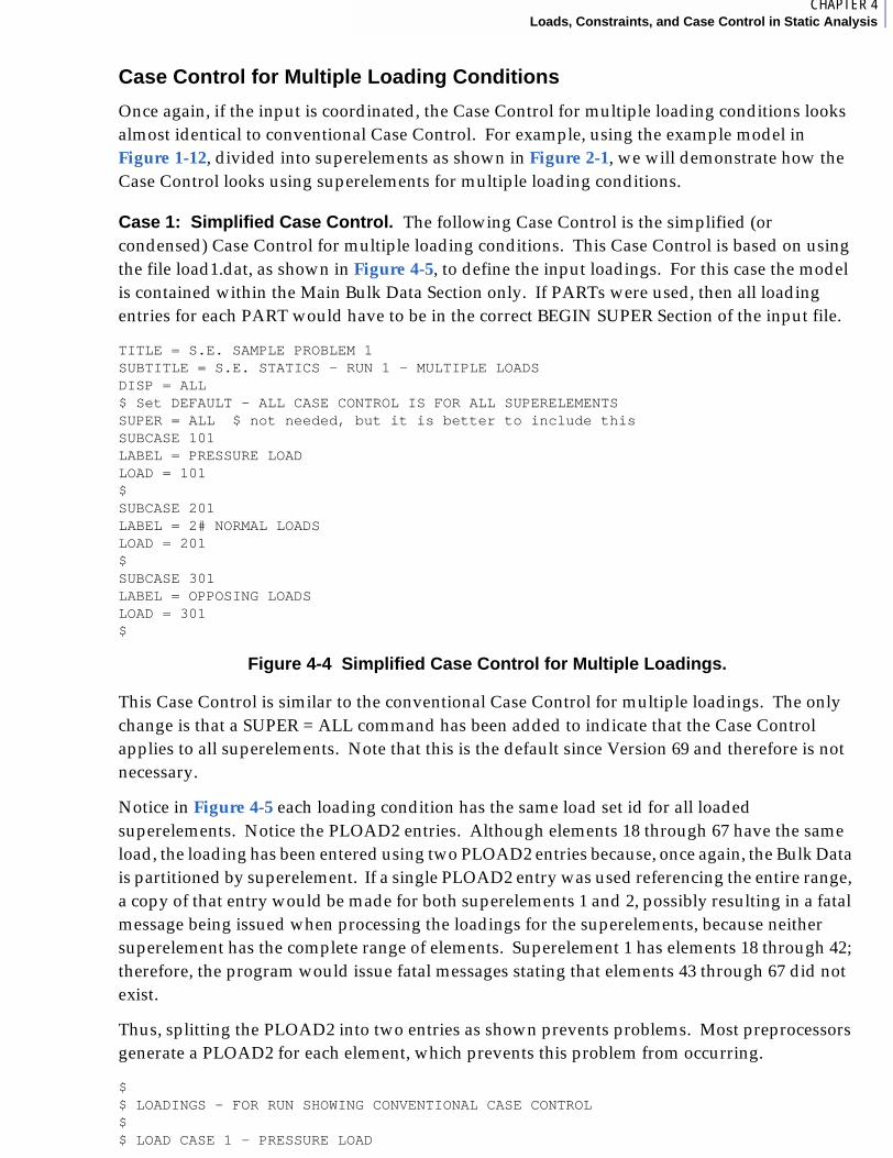
7CHAPTER 4Loads, Constraints, and Case Control in Static Analysis
Case Control for Multiple Loading Conditions
Once again, if the input is coordinated, the Case Control for multiple loading conditions looks almost identical to conventional Case Control. For example, using the example model in Figure 1-12, divided into superelements as shown in Figure 2-1, we will demonstrate how the Case Control looks using superelements for multiple loading conditions.
Case 1: Simplified Case Control. The following Case Control is the simplified (or condensed) Case Control for multiple loading conditions. This Case Control is based on using the file load1.dat, as shown in Figure 4-5, to define the input loadings. For this case the model is contained within the Main Bulk Data Section only. If PARTs were used, then all loading entries for each PART would have to be in the correct BEGIN SUPER Section of the input file.
TITLE = S.E. SAMPLE PROBLEM 1 SUBTITLE = S.E. STATICS - RUN 1 - MULTIPLE LOADSDISP = ALL$ Set DEFAULT - ALL CASE CONTROL IS FOR ALL SUPERELEMENTSSUPER = ALL $ not needed, but it is better to include thisSUBCASE 101LABEL = PRESSURE LOADLOAD = 101$SUBCASE 201LABEL = 2# NORMAL LOADSLOAD = 201$SUBCASE 301LABEL = OPPOSING LOADSLOAD = 301$
Figure 4-4 Simplified Case Control for Multiple Loadings.
This Case Control is similar to the conventional Case Control for multiple loadings. The only change is that a SUPER = ALL command has been added to indicate that the Case Control applies to all superelements. Note that this is the default since Version 69 and therefore is not necessary.
Notice in Figure 4-5 each loading condition has the same load set id for all loaded superelements. Notice the PLOAD2 entries. Although elements 18 through 67 have the same load, the loading has been entered using two PLOAD2 entries because, once again, the Bulk Data is partitioned by superelement. If a single PLOAD2 entry was used referencing the entire range, a copy of that entry would be made for both superelements 1 and 2, possibly resulting in a fatal message being issued when processing the loadings for the superelements, because neither superelement has the complete range of elements. Superelement 1 has elements 18 through 42; therefore, the program would issue fatal messages stating that elements 43 through 67 did not exist.
Thus, splitting the PLOAD2 into two entries as shown prevents problems. Most preprocessors generate a PLOAD2 for each element, which prevents this problem from occurring.
$$ LOADINGS - FOR RUN SHOWING CONVENTIONAL CASE CONTROL$$ LOAD CASE 1 - PRESSURE LOAD
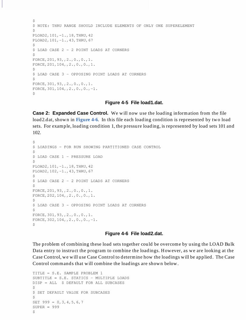
$$ NOTE: THRU RANGE SHOULD INCLUDE ELEMENTS OF ONLY ONE SUPERELEMENT$PLOAD2,101,-1.,18,THRU,42PLOAD2,101,-1.,43,THRU,67$$ LOAD CASE 2 - 2 POINT LOADS AT CORNERS$FORCE,201,93,,2.,0.,0.,1.FORCE,201,104,,2.,0.,0.,1.$$ LOAD CASE 3 - OPPOSING POINT LOADS AT CORNERS$FORCE,301,93,,2.,0.,0.,1.FORCE,301,104,,2.,0.,0.,-1.$
Figure 4-5 File load1.dat.
Case 2: Expanded Case Control. We will now use the loading information from the file load2.dat, shown in Figure 4-6. In this file each loading condition is represented by two load sets. For example, loading condition 1, the pressure loading, is represented by load sets 101 and 102.
$$ LOADINGS - FOR RUN SHOWING PARTITIONED CASE CONTROL$$ LOAD CASE 1 - PRESSURE LOAD$PLOAD2,101,-1.,18,THRU,42PLOAD2,102,-1.,43,THRU,67$$ LOAD CASE 2 - 2 POINT LOADS AT CORNERS$FORCE,201,93,,2.,0.,0.,1.FORCE,202,104,,2.,0.,0.,1.$$ LOAD CASE 3 - OPPOSING POINT LOADS AT CORNERS$FORCE,301,93,,2.,0.,0.,1.FORCE,302,104,,2.,0.,0.,-1.$
Figure 4-6 File load2.dat.
The problem of combining these load sets together could be overcome by using the LOAD Bulk Data entry to instruct the program to combine the loadings. However, as we are looking at the Case Control, we will use Case Control to determine how the loadings will be applied. The Case Control commands that will combine the loadings are shown below.
TITLE = S.E. SAMPLE PROBLEM 1 SUBTITLE = S.E. STATICS - MULTIPLE LOADSDISP = ALL $ DEFAULT FOR ALL SUBCASES$$ SET DEFAULT VALUE FOR SUBCASES$SET 999 = 0,3,4,5,6,7SUPER = 999$
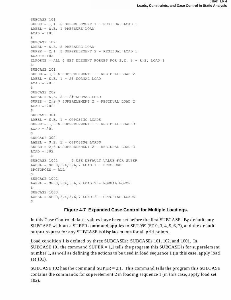
7CHAPTER 4Loads, Constraints, and Case Control in Static Analysis
SUBCASE 101SUPER = 1,1 $ SUPERELEMENT 1 - RESIDUAL LOAD 1LABEL = S.E. 1 PRESSURE LOADLOAD = 101$SUBCASE 102LABEL = S.E. 2 PRESSURE LOADSUPER = 2,1 $ SUPERELEMENT 2 - RESIDUAL LOAD 1LOAD = 102ELFORCE = ALL $ GET ELEMENT FORCES FOR S.E. 2 - R.S. LOAD 1$SUBCASE 201SUPER = 1,2 $ SUPERELEMENT 1 - RESIDUAL LOAD 2LABEL = S.E. 1 - 2# NORMAL LOADLOAD = 201$SUBCASE 202LABEL = S.E. 2 - 2# NORMAL LOADSUPER = 2,2 $ SUPERELEMENT 2 - RESIDUAL LOAD 2LOAD = 202$SUBCASE 301LABEL = S.E. 1 - OPPOSING LOADSSUPER = 1,3 $ SUPERELEMENT 1 - RESIDUAL LOAD 3LOAD = 301$SUBCASE 302LABEL = S.E. 2 - OPPOSING LOADSSUPER = 2,3 $ SUPERELEMENT 2 - RESIDUAL LOAD 3LOAD = 302$SUBCASE 1001 $ USE DEFAULT VALUE FOR SUPERLABEL = SE 0,3,4,5,6,7 LOAD 1 - PRESSURESPCFORCES = ALL$SUBCASE 1002LABEL = SE 0,3,4,5,6,7 LOAD 2 - NORMAL FORCE$SUBCASE 1003LABEL = SE 0,3,4,5,6,7 LOAD 3 - OPPOSING LOADS$
Figure 4-7 Expanded Case Control for Multiple Loadings.
In this Case Control default values have been set before the first SUBCASE. By default, any SUBCASE without a SUPER command applies to SET 999 (SE 0, 3, 4, 5, 6, 7), and the default output request for any SUBCASE is displacements for all grid points.
Load condition 1 is defined by three SUBCASEs: SUBCASEs 101, 102, and 1001. In SUBCASE 101 the command SUPER = 1,1 tells the program this SUBCASE is for superelement number 1, as well as defining the actions to be used in load sequence 1 (in this case, apply load set 101).
SUBCASE 102 has the command SUPER = 2,1. This command tells the program this SUBCASE contains the commands for superelement 2 in loading sequence 1 (in this case, apply load set 102).

SUBCASE 1001 has no SUPER command, thus MSC.Nastran uses the default assigned before the first SUBCASE, which applies to superelements 0, 3, 4, 5, 6, and 7. Because there is no load sequence number provided, the program assigns a load sequence number based on the order in which the SUBCASE appears. Because this is the first SUBCASE for these superelements, this SUBCASE is used for loading sequence 1, just as if we had entered the command SUPER = 999,1. No loadings are applied in this SUBCASE, so the only loadings for this loading condition are those applied to superelements 1 and 2.
Loading condition 2 is defined in a similar manner using SUBCASEs 201, 202, and 1002. Loading condition 3 is defined by SUBCASES 301, 302, and 1003.
A common omission in the Case Control Section is to forget to include a command for a superelement that has no loads or constraints applied to it. This omission will not cause incorrect answers but will prevent obtaining any output for that superelement for that loading condition.
In this example SUBCASEs 1001, 1002, and 1003 have been used to define the output requests for superelements 0, 3, 4, 5, 6, and 7. Note that if the SUPER=999 command had been omitted these SUBCASEs would apply only to the residual structure, and therefore, would not request any output for superelements 3, 4, 5, 6, or 7.
Second Example of Expanded Case Control
We will assume that the following model has been created by two separate engineering groups. One group (group A) has created the model for superelement 1. This group used load set 1 to define the first loading condition and loading set 2 to define the second loading condition. Another group (group B) has created the model that will be used as the residual structure. Unfortunately, due to a lack of communication, group B used load set 2 to define loading condition 1 and load set 1 to define loading condition 2.
In a conventional analysis this problem could not be solved without making changes to the Bulk Data, with the ensuing potential for error. By using the expanded Case Control and superelements, the original Bulk Data can be used without modification.
Note: Be careful--if no SUBCASE exists for a superelement for a loading, no loads are applied to that superelement for that loading and no output is available for that superelement for that loading.
Note: This condition can be corrected by adding a SUBCASE for the superelement on a restart run.
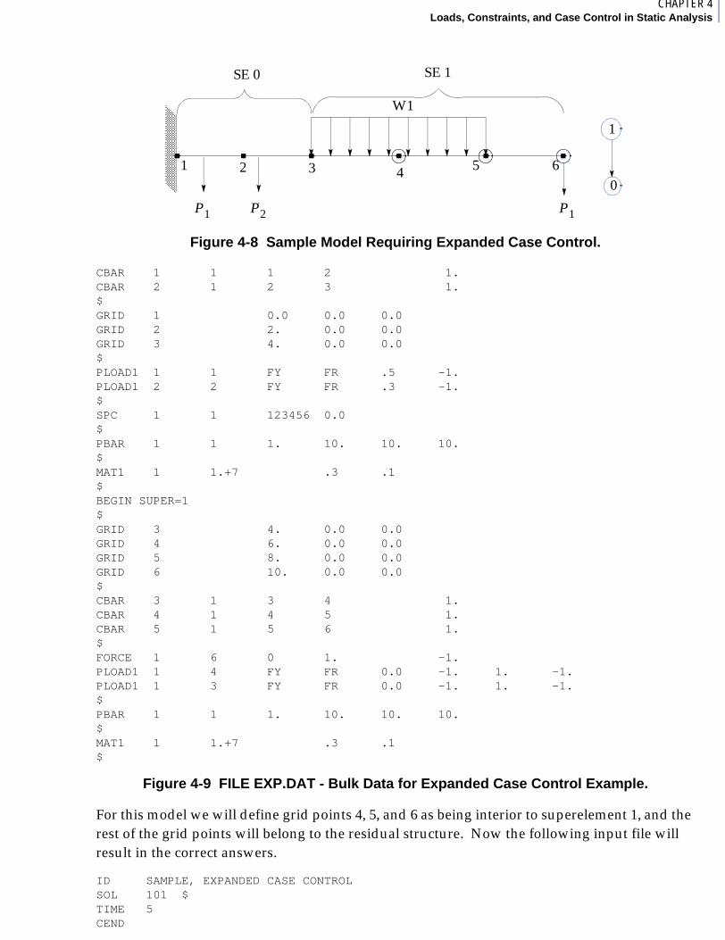
7CHAPTER 4Loads, Constraints, and Case Control in Static Analysis
Figure 4-8 Sample Model Requiring Expanded Case Control.
CBAR 1 1 1 2 1.CBAR 2 1 2 3 1.$GRID 1 0.0 0.0 0.0 GRID 2 2. 0.0 0.0 GRID 3 4. 0.0 0.0 $PLOAD1 1 1 FY FR .5 -1. PLOAD1 2 2 FY FR .3 -1. $SPC 1 1 123456 0.0 $PBAR 1 1 1. 10. 10. 10. $MAT1 1 1.+7 .3 .1 $BEGIN SUPER=1$GRID 3 4. 0.0 0.0 GRID 4 6. 0.0 0.0 GRID 5 8. 0.0 0.0 GRID 6 10. 0.0 0.0 $CBAR 3 1 3 4 1.CBAR 4 1 4 5 1.CBAR 5 1 5 6 1.$FORCE 1 6 0 1. -1. PLOAD1 1 4 FY FR 0.0 -1. 1. -1. PLOAD1 1 3 FY FR 0.0 -1. 1. -1. $PBAR 1 1 1. 10. 10. 10. $MAT1 1 1.+7 .3 .1 $
Figure 4-9 FILE EXP.DAT - Bulk Data for Expanded Case Control Example.
For this model we will define grid points 4, 5, and 6 as being interior to superelement 1, and the rest of the grid points will belong to the residual structure. Now the following input file will result in the correct answers.
ID SAMPLE, EXPANDED CASE CONTROLSOL 101 $TIME 5CEND
1
SE 0 SE 1
W1
1 2 3 4 5 60
P1 P2 P1
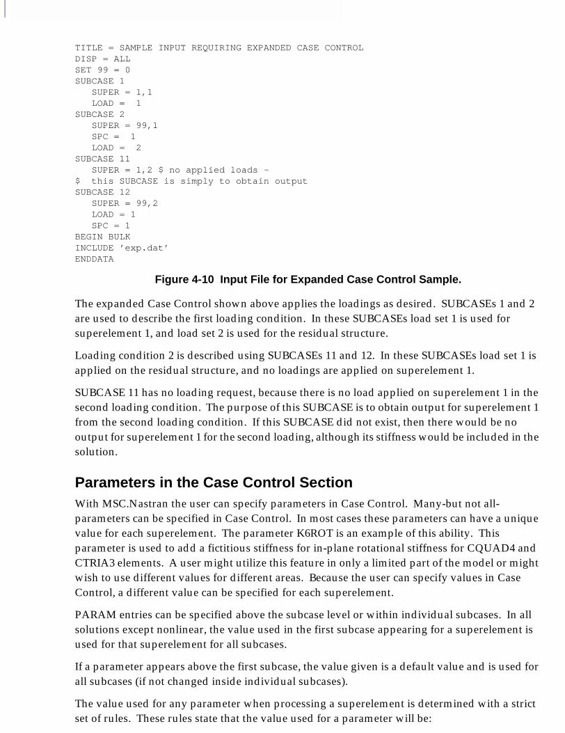
TITLE = SAMPLE INPUT REQUIRING EXPANDED CASE CONTROLDISP = ALLSET 99 = 0SUBCASE 1 SUPER = 1,1 LOAD = 1SUBCASE 2 SUPER = 99,1 SPC = 1 LOAD = 2SUBCASE 11 SUPER = 1,2 $ no applied loads - $ this SUBCASE is simply to obtain outputSUBCASE 12 SUPER = 99,2 LOAD = 1 SPC = 1BEGIN BULKINCLUDE ’exp.dat’ENDDATA
Figure 4-10 Input File for Expanded Case Control Sample.
The expanded Case Control shown above applies the loadings as desired. SUBCASEs 1 and 2 are used to describe the first loading condition. In these SUBCASEs load set 1 is used for superelement 1, and load set 2 is used for the residual structure.
Loading condition 2 is described using SUBCASEs 11 and 12. In these SUBCASEs load set 1 is applied on the residual structure, and no loadings are applied on superelement 1.
SUBCASE 11 has no loading request, because there is no load applied on superelement 1 in the second loading condition. The purpose of this SUBCASE is to obtain output for superelement 1 from the second loading condition. If this SUBCASE did not exist, then there would be no output for superelement 1 for the second loading, although its stiffness would be included in the solution.
Parameters in the Case Control SectionWith MSC.Nastran the user can specify parameters in Case Control. Many-but not all-parameters can be specified in Case Control. In most cases these parameters can have a unique value for each superelement. The parameter K6ROT is an example of this ability. This parameter is used to add a fictitious stiffness for in-plane rotational stiffness for CQUAD4 and CTRIA3 elements. A user might utilize this feature in only a limited part of the model or might wish to use different values for different areas. Because the user can specify values in Case Control, a different value can be specified for each superelement.
PARAM entries can be specified above the subcase level or within individual subcases. In all solutions except nonlinear, the value used in the first subcase appearing for a superelement is used for that superelement for all subcases.
If a parameter appears above the first subcase, the value given is a default value and is used for all subcases (if not changed inside individual subcases).
The value used for any parameter when processing a superelement is determined with a strict set of rules. These rules state that the value used for a parameter will be:
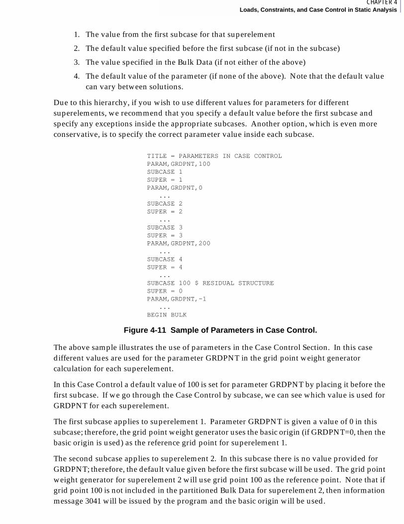
8CHAPTER 4Loads, Constraints, and Case Control in Static Analysis
1. The value from the first subcase for that superelement
2. The default value specified before the first subcase (if not in the subcase)
3. The value specified in the Bulk Data (if not either of the above)
4. The default value of the parameter (if none of the above). Note that the default value can vary between solutions.
Due to this hierarchy, if you wish to use different values for parameters for different superelements, we recommend that you specify a default value before the first subcase and specify any exceptions inside the appropriate subcases. Another option, which is even more conservative, is to specify the correct parameter value inside each subcase.
Figure 4-11 Sample of Parameters in Case Control.
The above sample illustrates the use of parameters in the Case Control Section. In this case different values are used for the parameter GRDPNT in the grid point weight generator calculation for each superelement.
In this Case Control a default value of 100 is set for parameter GRDPNT by placing it before the first subcase. If we go through the Case Control by subcase, we can see which value is used for GRDPNT for each superelement.
The first subcase applies to superelement 1. Parameter GRDPNT is given a value of 0 in this subcase; therefore, the grid point weight generator uses the basic origin (if GRDPNT=0, then the basic origin is used) as the reference grid point for superelement 1.
The second subcase applies to superelement 2. In this subcase there is no value provided for GRDPNT; therefore, the default value given before the first subcase will be used. The grid point weight generator for superelement 2 will use grid point 100 as the reference point. Note that if grid point 100 is not included in the partitioned Bulk Data for superelement 2, then information message 3041 will be issued by the program and the basic origin will be used.
TITLE = PARAMETERS IN CASE CONTROLPARAM,GRDPNT,100SUBCASE 1SUPER = 1PARAM,GRDPNT,0 ...SUBCASE 2SUPER = 2 ...SUBCASE 3SUPER = 3PARAM,GRDPNT,200 ...SUBCASE 4SUPER = 4 ...SUBCASE 100 $ RESIDUAL STRUCTURESUPER = 0PARAM,GRDPNT,-1 ...BEGIN BULK

The third subcase applies to superelement 3. Once again, a value is provided for GRDPNT in this subcase. The grid point weight generator output for superelement 3 will use grid point 200 as the reference grid point. (Once again, if grid 200 is not in the partitioned data for superelement 3, the basic origin will be used.)
The fourth subcase applies to superelement 4. No value is provided for GRDPNT in this subcase; therefore, the default value of 100 will be used.
The final subcase applies to the residual structure. In this subcase a value of -1 is provided for GRDPNT, meaning that the grid point weight generator will not be calculated for the residual structure.
Note: When processing superelements, the output from Grid Point Weight Generator will contain the current superelement only. Assembly weight is not printed.
MSC.Nastran Superelements User’s Guide
CHAPTER
5 Inertia Relief Analysis Using Superelements
■ Introduction
■ The Concept of Inertia Relief
■ Interface for Inertia Relief Using Superelements
■ Example of Inertia Relief Using Superelements

5.1 IntroductionInertia relief is a subset of static analysis. Inertia relief is normally used to allow static solution of models that are not stable. That is, if a structure has possible mechanisms or rigid body motion, a static analysis cannot be performed using conventional methods. Inertia relief provides an approach that can solve problems containing mechanisms or rigid body modes.
Refer to the following reference documentation for further description and theoretical discussion:
MSC.Nastran Common Questions and Answers - “Static Analysis” in Chapter 6
MSC.Nastran Linear Static Analysis User’s Guide - “Inertia Relief” in Chapter 11
MSC.Nastran Reference Manual - “Solution Sequences” in Chapter 7

8CHAPTER 5Inertia Relief Analysis Using Superelements
5.2 The Concept of Inertia ReliefWhen using inertia relief, you want to obtain a static solution for a structure that is not stable, but is in a state of equilibrium under loading. Examples of structures in this state are aircraft in flight, cars in motion, and spacecraft in orbit. Each of these structures has one or more unconstrained, rigid body motions possible. Therefore, it is not possible to solve these problems using conventional static analysis. In inertia relief the structure is in a state of static equilibrium under applied loading and inertial loads.
When inertia relief is invoked, the program will calculate the summation of all loads and the mass properties about the reference degrees-of-freedom (DOFs), and then the inertial loads required to put the structure in a state of static equilibrium will be calculated. The program applies the static loads and these accelerations simultaneously. The model is now in a state of equilibrium, and a set of constraints must be added that can prevent any rigid body motion or mechanisms. The program accomplishes this task by constraining the reference DOFs and performing the solution. If the structure is capable of rigid body motion or mechanisms and the reference DOFs can prevent these, then the reaction forces at the reference DOFs will be zero.
The implementation of inertia relief in SOL 1 is a general implementation and allows for any number and combination of rigid-body modes and mechanisms.
The implementation in SOL 101 (superelements) is different. A maximum of six reference DOFs can be specified. The intent is to allow the solution of structures that are not constrained (or to allow rigid body motion) and not mechanisms. At the superelement level, SOL 101 calculates additional loadings (beyond those specified in the Case Control Section). Each of these loads corresponds to a unit acceleration of the superelement mass about the reference point (PARAM,GRDPNT). The procedure used to solve the inertia relief problem is described in the “Solution Sequences” on page 341 of the MSC.Nastran Reference Guide.

5.3 Interface for Inertia Relief Using SuperelementsIn SOL 101 inertia relief is invoked by using a SUPORT entry and PARAM,INREL,-1. If a SUPORT entry is used and PARAM,INREL is not set to -1, the program will perform a static solution with the reference (SUPORT) DOFs constrained and will not calculate the acceleration loads required for equilibrium.
PARAM,GRDPNT if used in a run using inertial relief, must be specified for all superelements, and the location of the reference grid point must be identical for all superelements.
An additional Bulk Data entry, DMIG,UACCEL, is available so user-specified accelerations can be used in place of the ones calculated for equilibrium. If this entry is used, you must specify the point about which the accelerations will be applied (this point must appear on a SUPORT entry), and you must specify the accelerations to be applied for each solution (SUBCASE).
The SUPORT entry, PARAM,INREL,-1, and the DMIG UACCEL entries must be in the Main Bulk Data Section, and they must point to grid points that are in the residual structure.
If PARTs are used for inertia relief, PARAM,INREL,-1 must appear in the bulk data for each PART and in the main bulk data.
PARAM,GRDPNT can be used to provide the location to sum the mass properties when calculating the accelerations, but if PARAM,GRDPNT is used it should be specified for each superelement. If GRDPNT references a point that is not in a superelement, the program will terminate with User Fatal Message 9006.
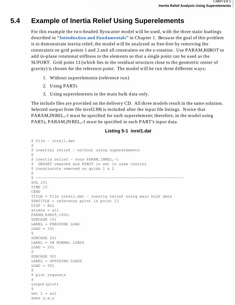
8CHAPTER 5Inertia Relief Analysis Using Superelements
5.4 Example of Inertia Relief Using SuperelementsFor this example the two-headed flyswatter model will be used, with the three static loadings described in “Introduction and Fundamentals” in Chapter 1. Because the goal of this problem is to demonstrate inertia relief, the model will be analyzed as free-free by removing the constraints on grid points 1 and 2 and all constraints on the z-rotation. Use PARAM,K6ROT to add in-plane rotational stiffness to the elements so that a single point can be used as the SUPORT. Grid point 13 (which lies in the residual structure close to the geometric center of gravity) is chosen for the reference point. The model will be run three different ways:
1. Without superelements (reference run)
2. Using PARTs
3. Using superelements in the main bulk data only.
The include files are provided on the delivery CD. All three models result in the same solution. Selected output from file inrel2.f06 is included after the input file listings. Notice that PARAM,INREL,-1 must be specified for each superelement; therefore, in the model using PARTs, PARAM,INREL,-1 must be specified in each PART’s input data.
Listing 5-1 inrel1.dat
$ file - inrel1.dat $ $ inertial relief - without using superelements$$ inertia relief - note PARAM,INREL,-1 $ GRDSET removed and K6ROT is set in case control$ constraints removed on grids 1 & 2$$ ----------------------------------------------------------------SOL 101 TIME 15CENDTITLE = File inrel1.dat - inertia relief using main bulk dataSUBTITLE = reference point is point 13 DISP = ALLstress = allPARAM,K6ROT,1000.SUBCASE 101LABEL = PRESSURE LOADLOAD = 101$SUBCASE 201LABEL = 2# NORMAL LOADSLOAD = 201$SUBCASE 301LABEL = OPPOSING LOADSLOAD = 301$$ plot requests$output(plot)$set 1 = allaxes z,x,y
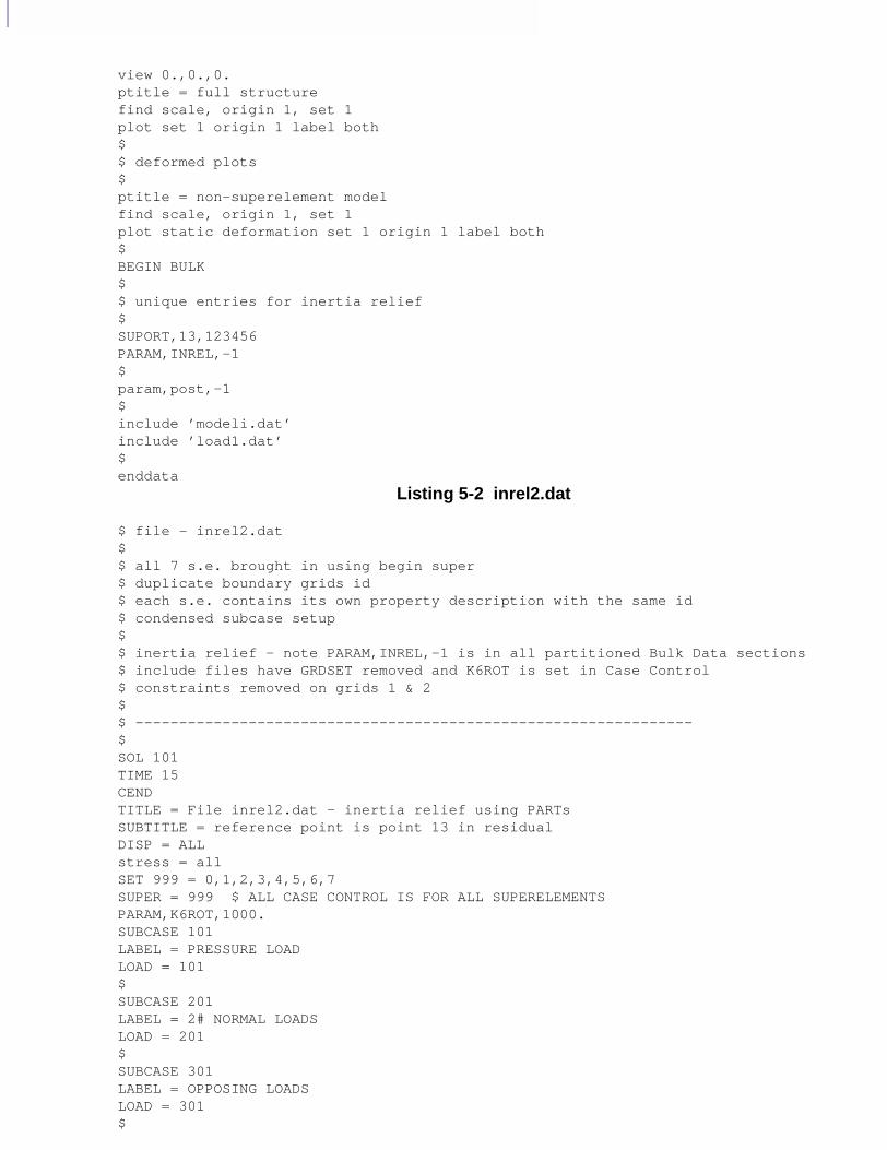
view 0.,0.,0.ptitle = full structurefind scale, origin 1, set 1plot set 1 origin 1 label both$$ deformed plots$ptitle = non-superelement modelfind scale, origin 1, set 1plot static deformation set 1 origin 1 label both$BEGIN BULK$$ unique entries for inertia relief$SUPORT,13,123456PARAM,INREL,-1$param,post,-1$include ’modeli.dat’include ’load1.dat’$ enddata
Listing 5-2 inrel2.dat
$ file - inrel2.dat $ $ all 7 s.e. brought in using begin super$ duplicate boundary grids id$ each s.e. contains its own property description with the same id$ condensed subcase setup$$ inertia relief - note PARAM,INREL,-1 is in all partitioned Bulk Data sections$ include files have GRDSET removed and K6ROT is set in Case Control$ constraints removed on grids 1 & 2$$ ----------------------------------------------------------------$SOL 101 TIME 15CENDTITLE = File inrel2.dat - inertia relief using PARTsSUBTITLE = reference point is point 13 in residualDISP = ALLstress = allSET 999 = 0,1,2,3,4,5,6,7SUPER = 999 $ ALL CASE CONTROL IS FOR ALL SUPERELEMENTSPARAM,K6ROT,1000.SUBCASE 101LABEL = PRESSURE LOADLOAD = 101$SUBCASE 201LABEL = 2# NORMAL LOADSLOAD = 201$SUBCASE 301LABEL = OPPOSING LOADSLOAD = 301$
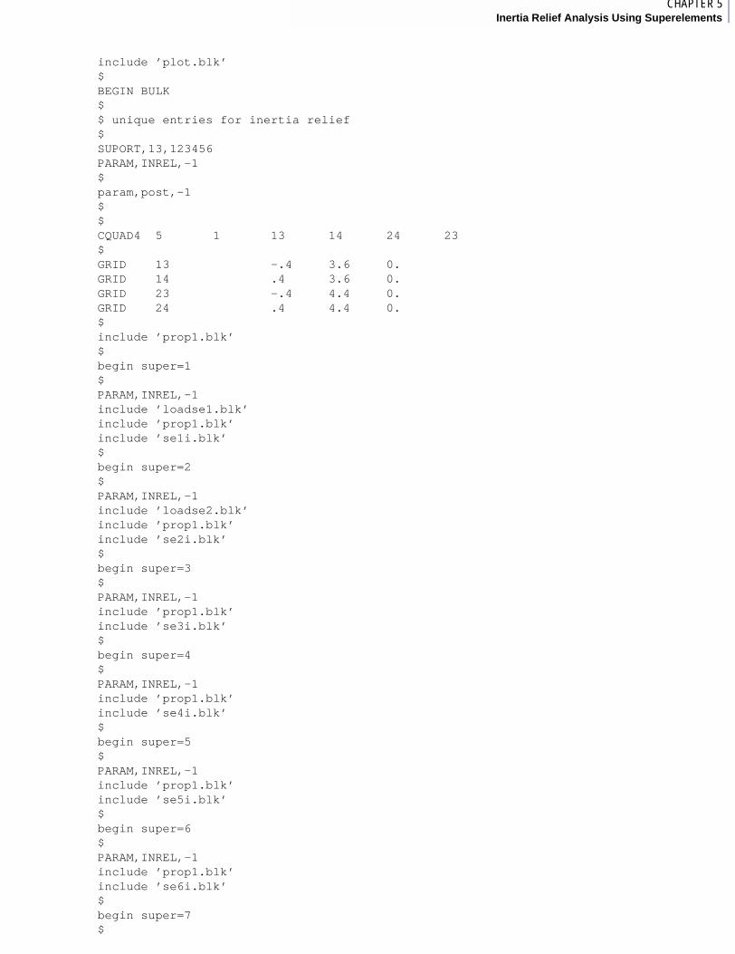
8CHAPTER 5Inertia Relief Analysis Using Superelements
include ’plot.blk’$BEGIN BULK$$ unique entries for inertia relief$SUPORT,13,123456PARAM,INREL,-1$param,post,-1$$ CQUAD4 5 1 13 14 24 23 $GRID 13 -.4 3.6 0. GRID 14 .4 3.6 0. GRID 23 -.4 4.4 0. GRID 24 .4 4.4 0. $include ’prop1.blk’$begin super=1$PARAM,INREL,-1include ’loadse1.blk’include ’prop1.blk’include ’se1i.blk’$begin super=2$ PARAM,INREL,-1include ’loadse2.blk’include ’prop1.blk’include ’se2i.blk’$begin super=3$ PARAM,INREL,-1include ’prop1.blk’include ’se3i.blk’$begin super=4$ PARAM,INREL,-1include ’prop1.blk’include ’se4i.blk’$begin super=5$ PARAM,INREL,-1include ’prop1.blk’include ’se5i.blk’$begin super=6$ PARAM,INREL,-1include ’prop1.blk’include ’se6i.blk’$begin super=7$
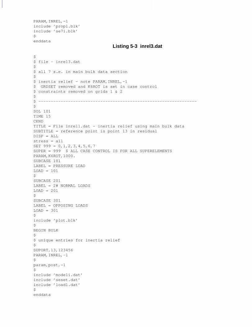
PARAM,INREL,-1include ’prop1.blk’include ’se7i.blk’ $enddata
Listing 5-3 inrel3.dat
$$ file - inrel3.dat $ $ all 7 s.e. in main bulk data section $$ inertia relief - note PARAM,INREL,-1 $ GRDSET removed and K6ROT is set in case control$ constraints removed on grids 1 & 2$$ ----------------------------------------------------------------$SOL 101 TIME 15CENDTITLE = File inrel1.dat - inertia relief using main bulk dataSUBTITLE = reference point is point 13 in residualDISP = ALLstress = allSET 999 = 0,1,2,3,4,5,6,7SUPER = 999 $ ALL CASE CONTROL IS FOR ALL SUPERELEMENTSPARAM,K6ROT,1000.SUBCASE 101LABEL = PRESSURE LOADLOAD = 101$SUBCASE 201LABEL = 2# NORMAL LOADSLOAD = 201$SUBCASE 301LABEL = OPPOSING LOADSLOAD = 301$include ’plot.blk’$BEGIN BULK$$ unique entries for inertia relief$SUPORT,13,123456PARAM,INREL,-1$param,post,-1 $include ’modeli.dat’include ’seset.dat’include ’load1.dat’$ enddata
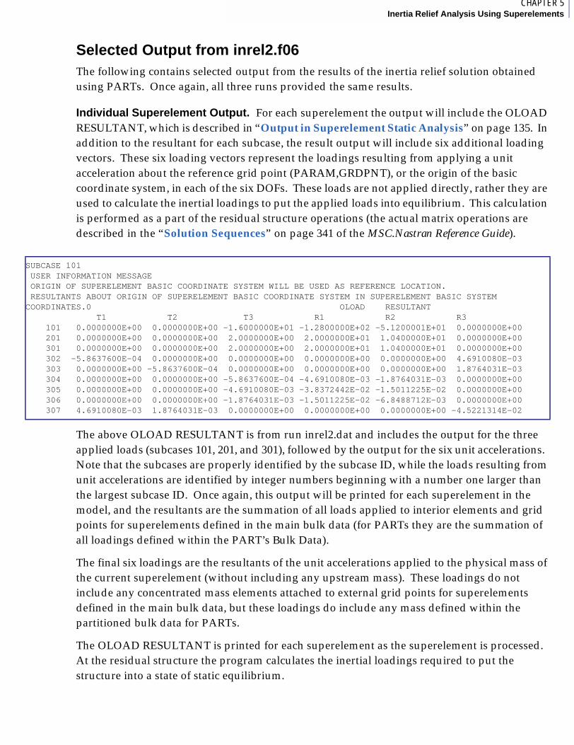
9CHAPTER 5Inertia Relief Analysis Using Superelements
Selected Output from inrel2.f06The following contains selected output from the results of the inertia relief solution obtained using PARTs. Once again, all three runs provided the same results.
Individual Superelement Output. For each superelement the output will include the OLOAD RESULTANT, which is described in “Output in Superelement Static Analysis” on page 135. In addition to the resultant for each subcase, the result output will include six additional loading vectors. These six loading vectors represent the loadings resulting from applying a unit acceleration about the reference grid point (PARAM,GRDPNT), or the origin of the basic coordinate system, in each of the six DOFs. These loads are not applied directly, rather they are used to calculate the inertial loadings to put the applied loads into equilibrium. This calculation is performed as a part of the residual structure operations (the actual matrix operations are described in the “Solution Sequences” on page 341 of the MSC.Nastran Reference Guide).
The above OLOAD RESULTANT is from run inrel2.dat and includes the output for the three applied loads (subcases 101, 201, and 301), followed by the output for the six unit accelerations. Note that the subcases are properly identified by the subcase ID, while the loads resulting from unit accelerations are identified by integer numbers beginning with a number one larger than the largest subcase ID. Once again, this output will be printed for each superelement in the model, and the resultants are the summation of all loads applied to interior elements and grid points for superelements defined in the main bulk data (for PARTs they are the summation of all loadings defined within the PART’s Bulk Data).
The final six loadings are the resultants of the unit accelerations applied to the physical mass of the current superelement (without including any upstream mass). These loadings do not include any concentrated mass elements attached to external grid points for superelements defined in the main bulk data, but these loadings do include any mass defined within the partitioned bulk data for PARTs.
The OLOAD RESULTANT is printed for each superelement as the superelement is processed. At the residual structure the program calculates the inertial loadings required to put the structure into a state of static equilibrium.
SUBCASE 101 USER INFORMATION MESSAGE ORIGIN OF SUPERELEMENT BASIC COORDINATE SYSTEM WILL BE USED AS REFERENCE LOCATION. RESULTANTS ABOUT ORIGIN OF SUPERELEMENT BASIC COORDINATE SYSTEM IN SUPERELEMENT BASIC SYSTEM COORDINATES.0 OLOAD RESULTANT T1 T2 T3 R1 R2 R3 101 0.0000000E+00 0.0000000E+00 -1.6000000E+01 -1.2800000E+02 -5.1200001E+01 0.0000000E+00 201 0.0000000E+00 0.0000000E+00 2.0000000E+00 2.0000000E+01 1.0400000E+01 0.0000000E+00 301 0.0000000E+00 0.0000000E+00 2.0000000E+00 2.0000000E+01 1.0400000E+01 0.0000000E+00 302 -5.8637600E-04 0.0000000E+00 0.0000000E+00 0.0000000E+00 0.0000000E+00 4.6910080E-03 303 0.0000000E+00 -5.8637600E-04 0.0000000E+00 0.0000000E+00 0.0000000E+00 1.8764031E-03 304 0.0000000E+00 0.0000000E+00 -5.8637600E-04 -4.6910080E-03 -1.8764031E-03 0.0000000E+00 305 0.0000000E+00 0.0000000E+00 -4.6910080E-03 -3.8372442E-02 -1.5011225E-02 0.0000000E+00 306 0.0000000E+00 0.0000000E+00 -1.8764031E-03 -1.5011225E-02 -6.8488712E-03 0.0000000E+00 307 4.6910080E-03 1.8764031E-03 0.0000000E+00 0.0000000E+00 0.0000000E+00 -4.5221314E-02
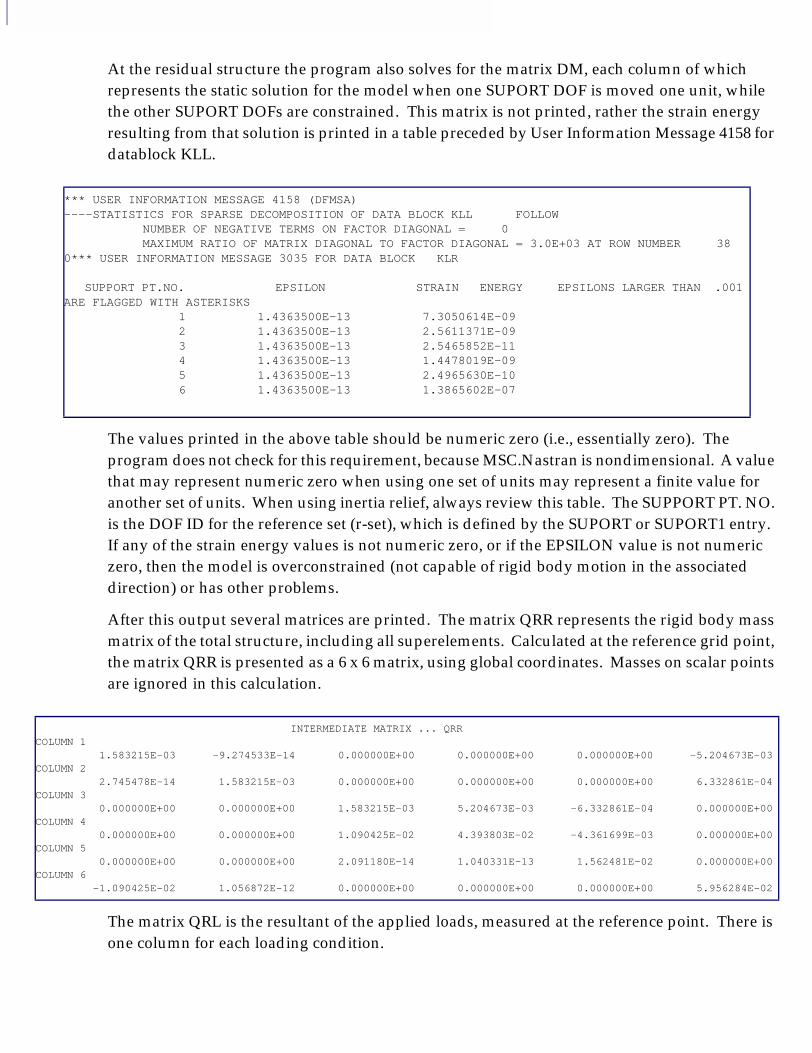
At the residual structure the program also solves for the matrix DM, each column of which represents the static solution for the model when one SUPORT DOF is moved one unit, while the other SUPORT DOFs are constrained. This matrix is not printed, rather the strain energy resulting from that solution is printed in a table preceded by User Information Message 4158 for datablock KLL.
The values printed in the above table should be numeric zero (i.e., essentially zero). The program does not check for this requirement, because MSC.Nastran is nondimensional. A value that may represent numeric zero when using one set of units may represent a finite value for another set of units. When using inertia relief, always review this table. The SUPPORT PT. NO. is the DOF ID for the reference set (r-set), which is defined by the SUPORT or SUPORT1 entry. If any of the strain energy values is not numeric zero, or if the EPSILON value is not numeric zero, then the model is overconstrained (not capable of rigid body motion in the associated direction) or has other problems.
After this output several matrices are printed. The matrix QRR represents the rigid body mass matrix of the total structure, including all superelements. Calculated at the reference grid point, the matrix QRR is presented as a 6 x 6 matrix, using global coordinates. Masses on scalar points are ignored in this calculation.
The matrix QRL is the resultant of the applied loads, measured at the reference point. There is one column for each loading condition.
*** USER INFORMATION MESSAGE 4158 (DFMSA)----STATISTICS FOR SPARSE DECOMPOSITION OF DATA BLOCK KLL FOLLOW NUMBER OF NEGATIVE TERMS ON FACTOR DIAGONAL = 0 MAXIMUM RATIO OF MATRIX DIAGONAL TO FACTOR DIAGONAL = 3.0E+03 AT ROW NUMBER 380*** USER INFORMATION MESSAGE 3035 FOR DATA BLOCK KLR
SUPPORT PT.NO. EPSILON STRAIN ENERGY EPSILONS LARGER THAN .001 ARE FLAGGED WITH ASTERISKS 1 1.4363500E-13 7.3050614E-09 2 1.4363500E-13 2.5611371E-09 3 1.4363500E-13 2.5465852E-11 4 1.4363500E-13 1.4478019E-09 5 1.4363500E-13 2.4965630E-10 6 1.4363500E-13 1.3865602E-07
INTERMEDIATE MATRIX ... QRRCOLUMN 1
1.583215E-03 -9.274533E-14 0.000000E+00 0.000000E+00 0.000000E+00 -5.204673E-03 COLUMN 2
2.745478E-14 1.583215E-03 0.000000E+00 0.000000E+00 0.000000E+00 6.332861E-04 COLUMN 3
0.000000E+00 0.000000E+00 1.583215E-03 5.204673E-03 -6.332861E-04 0.000000E+00 COLUMN 4
0.000000E+00 0.000000E+00 1.090425E-02 4.393803E-02 -4.361699E-03 0.000000E+00 COLUMN 5
0.000000E+00 0.000000E+00 2.091180E-14 1.040331E-13 1.562481E-02 0.000000E+00 COLUMN 6
-1.090425E-02 1.056872E-12 0.000000E+00 0.000000E+00 0.000000E+00 5.956284E-02

9CHAPTER 5Inertia Relief Analysis Using Superelements
The matrix URACCEL (not produced in this example) is the user-supplied rigid body acceleration, which is input on the DMlG,UACCEL entry. This output does not appear if the entry is not present.
The matrix URA represents the rigid body acceleration matrix, computed from the applied loads. Once these accelerations are computed, inertial loads are computed that will place the structure into a state of static equilibrium.
Once the inertial loads required to produce a state of static equilibrium are calculated, these inertial loads are applied and combined with the applied loads. The program then constrains the SUPORT (reference) DOFs and performs a static solution. The output from this point on is conventional superelement output.
0 SUBCASE 101 INTERMEDIATE MATRIX ... QRL COLUMN 1
0.000000E+00 0.000000E+00 3.200000E+01 1.408000E+02 -1.280000E+01 0.000000E+00 COLUMN 2
0.000000E+00 0.000000E+00 -4.000000E+00 -2.560000E+01 1.600000E+00 0.000000E+00 COLUMN 3
0.000000E+00 0.000000E+00 -3.758416E-11 -1.821405E-10 -2.080000E+01 0.000000E+00
INTERMEDIATE MATRIX ... URACOLUMN 1
0.000000E+00 0.000000E+00 1.009351E+04 -4.400139E+03 -6.921340E-10 0.000000E+00 COLUMN 2
0.000000E+00 0.000000E+00 -8.071358E+03 1.538730E+03 5.292301E-09 0.000000E+00 COLUMN 3
0.000000E+00 0.000000E+00 -3.727374E-09 1.434969E-09 1.331216E+03 0.000000E+00

MSC.Nastran Superelements User’s Guide
CHAPTER
6 Multiple Loadings in Static Analysis
■ Introduction
■ How Case Control is Internally Partitioned and Used
■ Examples for Multiple Loading Conditions

6.1 IntroductionAlthough “Loads, Constraints, and Case Control in Static Analysis” on page 61 discussed multiple loadings, this chapter clarifies how the Case Control is handled in static analysis with multiple loading conditions.
If multiple load cases exist in a static solution, a separate subcase must exist for the residual structure for each load condition or boundary condition. Separate subcases can exist for the superelements for each solution. Once again, MSC.Software recommends that either SUPER=ALL (the default) or separate subcases for each superelement for each solution should exist. This section describes how the program internally partitions the Case Control into separate sections for each superelement.

9CHAPTER 6Multiple Loadings in Static Analysis
6.2 How Case Control is Internally Partitioned and UsedWhen MSC.Nastran is processing your input file, as has already been mentioned, the Bulk Data is divided into separate sections (internal tables) based on your superelement definitions. In addition, the Case Control is also partitioned into separate sets for each superelement. (The name of this separate datablock is CASES in the DMAP.) You have already seen how the SUPER command is used to determine which SUBCASEs apply to which superelements. This command is also used in partitioning the Case Control.
Based on your use of the SUPER command, a separate set of Case Control is created for each superelement. One set is for the residual structure. You could think of the residual set as the master set of Case Control, which is controlling the actual solution. Once again, a SUBCASE must be defined for the residual structure for each loading condition (or boundary condition) you wish to solve. As mentioned before, the program actually copies any SUBCASEs that reference superelement 0 into a CASES table, which is qualified with SEID = 0. When processing the residual structure (PHASE 1), the program uses this copy of the Case Control.
The program creates a separate CASES table for each superelement in the model. The SEP2CT module creates this table during execution of the PHASE0 subDMAP in the program.
The following example shows (in an idealized form) the Case Control partitioning.
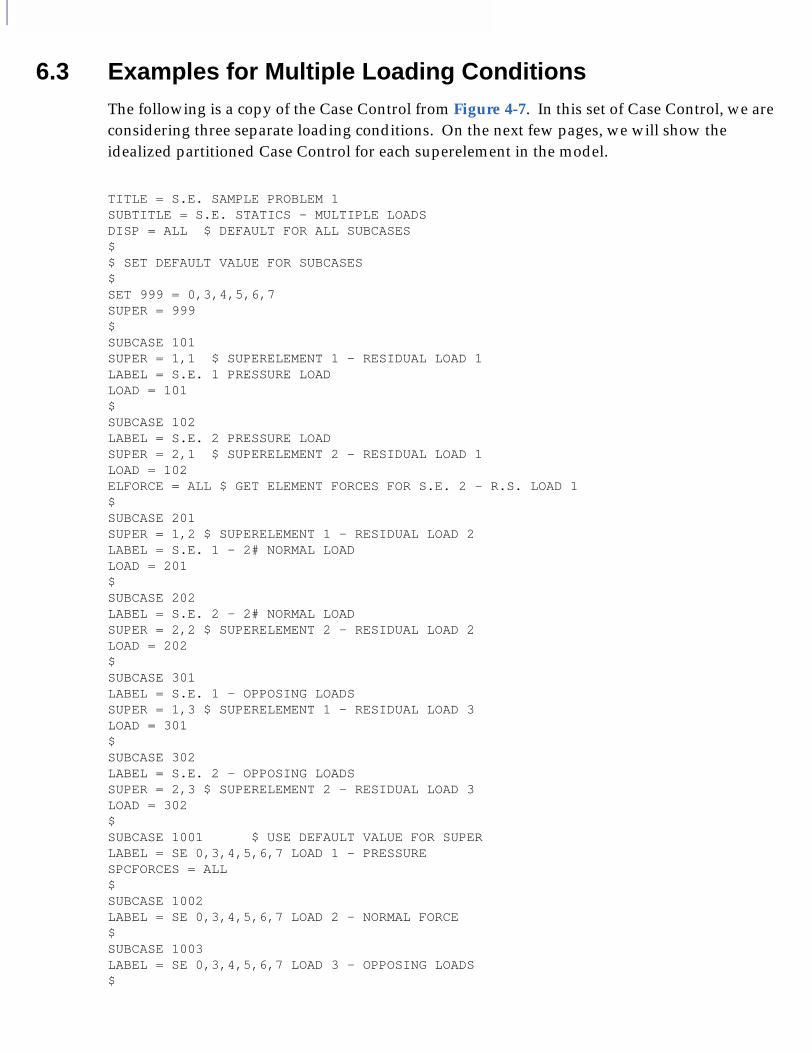
6.3 Examples for Multiple Loading ConditionsThe following is a copy of the Case Control from Figure 4-7. In this set of Case Control, we are considering three separate loading conditions. On the next few pages, we will show the idealized partitioned Case Control for each superelement in the model.
TITLE = S.E. SAMPLE PROBLEM 1 SUBTITLE = S.E. STATICS - MULTIPLE LOADSDISP = ALL $ DEFAULT FOR ALL SUBCASES$$ SET DEFAULT VALUE FOR SUBCASES$SET 999 = 0,3,4,5,6,7SUPER = 999$SUBCASE 101SUPER = 1,1 $ SUPERELEMENT 1 - RESIDUAL LOAD 1LABEL = S.E. 1 PRESSURE LOADLOAD = 101$SUBCASE 102LABEL = S.E. 2 PRESSURE LOADSUPER = 2,1 $ SUPERELEMENT 2 - RESIDUAL LOAD 1LOAD = 102ELFORCE = ALL $ GET ELEMENT FORCES FOR S.E. 2 - R.S. LOAD 1$SUBCASE 201SUPER = 1,2 $ SUPERELEMENT 1 - RESIDUAL LOAD 2LABEL = S.E. 1 - 2# NORMAL LOADLOAD = 201$SUBCASE 202LABEL = S.E. 2 - 2# NORMAL LOADSUPER = 2,2 $ SUPERELEMENT 2 - RESIDUAL LOAD 2LOAD = 202$SUBCASE 301LABEL = S.E. 1 - OPPOSING LOADSSUPER = 1,3 $ SUPERELEMENT 1 - RESIDUAL LOAD 3LOAD = 301$SUBCASE 302LABEL = S.E. 2 - OPPOSING LOADSSUPER = 2,3 $ SUPERELEMENT 2 - RESIDUAL LOAD 3LOAD = 302$SUBCASE 1001 $ USE DEFAULT VALUE FOR SUPERLABEL = SE 0,3,4,5,6,7 LOAD 1 - PRESSURESPCFORCES = ALL$SUBCASE 1002LABEL = SE 0,3,4,5,6,7 LOAD 2 - NORMAL FORCE$SUBCASE 1003LABEL = SE 0,3,4,5,6,7 LOAD 3 - OPPOSING LOADS$

9CHAPTER 6Multiple Loadings in Static Analysis
Idealized form of the CASES table (CASE CONTROL) for the residual structure (SE 0)-the copies for superelements 3, 4, 5, 6, and 7 are identical. SUBCASEs 1001, 1002, and 1003 do not contain a SUPER command, so they will get the default value of SUPER = 0,3,4,5,6,7 from above the SUBCASEs.
TITLE = S.E. SAMPLE PROBLEM 1 SUBTITLE = S.E. STATICS - MULTIPLE LOADSDISP = ALL $ DEFAULT FOR ALL SUBCASES$SUBCASE 1001 $ USE DEFAULT VALUE FOR SUPERLABEL = SE 0,3,4,5,6,7 LOAD 1 - PRESSURESPCFORCES = ALL$SUBCASE 1002LABEL = SE 0,3,4,5,6,7 LOAD 2 - NORMAL FORCE$SUBCASE 1003LABEL = SE 0,3,4,5,6,7 LOAD 3 - OPPOSING LOADS$
Idealized form of the CASES table (CASE CONTROL) for superelement 1.- SUBCASEs 101, 201, and 301 contain SUPER commands pointing to superelement 1, so they are placed in the CASES table for this superelement.
TITLE = S.E. SAMPLE PROBLEM 1 SUBTITLE = S.E. STATICS - MULTIPLE LOADSDISP = ALL $ DEFAULT FOR ALL SUBCASES$SUBCASE 101SUPER = 1,1 $ SUPERELEMENT 1 - RESIDUAL LOAD 1LABEL = S.E. 1 PRESSURE LOADLOAD = 101$SUBCASE 201SUPER = 1,2 $ SUPERELEMENT 1 - RESIDUAL LOAD 2LABEL = S.E. 1 - 2# NORMAL LOADLOAD = 201$SUBCASE 301LABEL = S.E. 1 - OPPOSING LOADSSUPER = 1,3 $ SUPERELEMENT 1 - RESIDUAL LOAD 3LOAD = 301$
Idealized form of the CASES table (CASE CONTROL) for superelement 2.- SUBCASEs 102, 202, and 302 contain SUPER commands pointing to superelement 2, so they are placed in the CASES table for this superelement.
TITLE = S.E. SAMPLE PROBLEM 1 SUBTITLE = S.E. STATICS - MULTIPLE LOADSDISP = ALL $ DEFAULT FOR ALL SUBCASES$SUBCASE 102LABEL = S.E. 2 PRESSURE LOAD

SUPER = 2,1 $ SUPERELEMENT 2 - RESIDUAL LOAD 1LOAD = 102ELFORCE = ALL $ GET ELEMENT FORCES FOR S.E. 2 - R.S. LOAD 1$SUBCASE 202LABEL = S.E. 2 - 2# NORMAL LOADSUPER = 2,2 $ SUPERELEMENT 2 - RESIDUAL LOAD 2LOAD = 202SUBCASE 302LABEL = S.E. 2 - OPPOSING LOADSSUPER = 2,3 $ SUPERELEMENT 2 - RESIDUAL LOAD 3LOAD = 302$
When performing the solution of this problem, the program combines the first SUBCASEs for each superelement to get the first solution, the second SUBCASEs for each superelement to get the second solution, etc. for as many solutions as are requested.
Therefore, the first solution is a combination of SUBCASE 101 (applied on superelement 1), SUBCASE 102 (applied on superelement 2), and SUBCASE 1001 (applied on superelements 3, 4, 5, 6, 7, and the residual structure).
Hopefully, this explanation will help you understand how the program combines the superelements and obtains the desired solutions. When we get to the section on dynamic analysis, this section will be a valuable reference.

MSC.Nastran Superelements User’s Guide
CHAPTER
7 Multilevel Superelement Analysis
■ The Concept of Multilevel Analysis
■ Comparison of Single- and Multilevel Analysis
■ User Interface for Multilevel Superelements
■ Example: Multilevel Problem Solved by Hand
■ Examples of Multilevel Superelements

7.1 The Concept of Multilevel AnalysisMultilevel superelement analysis occurs when one or more points which are exterior points of any superelement are interior to another superelement. If this is the case, then a single-level tree is no longer possible. That is, the information resulting from one (or more) superelement(s) is necessary to process another superelement.
In a single-level analysis, all superelements can be processed independently of each other; however, all superelements have to be processed before the residual structure can be processed. In multilevel analysis that requirement still exists, but it is possible to create assemblies of superelements. That is, the exterior points of several superelements can be interior to a downstream collector superelement that will then create an assembly.
Single-level analysis is the default approach if PARTs are used. You can only use multilevel analysis in a model that contains PARTs by either using the SETREE Bulk Data entry or the DTI,SETREE Bulk Data entry. See “User Interface for Multilevel Superelements” on page 119 for a description of these entries and how they are used.
If the model consists of main Bulk Data superelements only, the program checks to see that all exterior points belong to the residual structure before performing a single-level analysis. If a model is defined using the main Bulk Data only and exterior points exist that do not belong to the residual structure, then the program automatically performs a multilevel analysis. The SETREE and DTI,SETREE entries can also be used, in this case, to control the processing order and connectivity of the superelements.
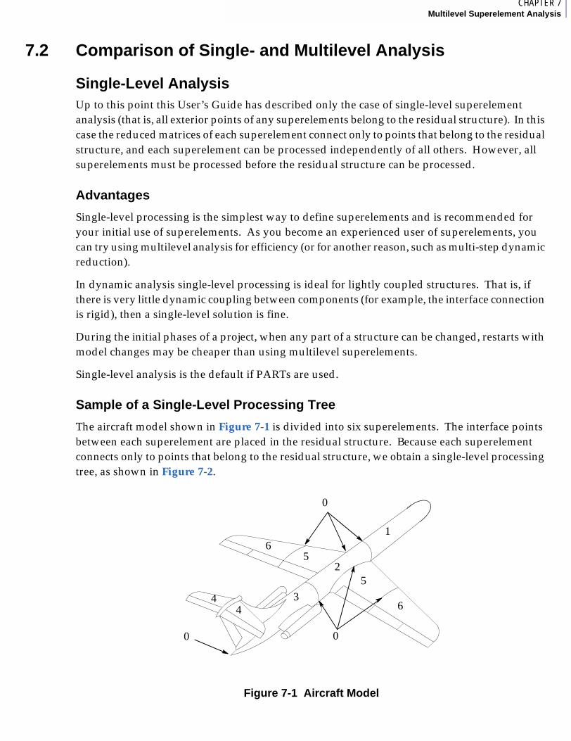
1CHAPTER 7Multilevel Superelement Analysis
7.2 Comparison of Single- and Multilevel Analysis
Single-Level AnalysisUp to this point this User’s Guide has described only the case of single-level superelement analysis (that is, all exterior points of any superelements belong to the residual structure). In this case the reduced matrices of each superelement connect only to points that belong to the residual structure, and each superelement can be processed independently of all others. However, all superelements must be processed before the residual structure can be processed.
Advantages
Single-level processing is the simplest way to define superelements and is recommended for your initial use of superelements. As you become an experienced user of superelements, you can try using multilevel analysis for efficiency (or for another reason, such as multi-step dynamic reduction).
In dynamic analysis single-level processing is ideal for lightly coupled structures. That is, if there is very little dynamic coupling between components (for example, the interface connection is rigid), then a single-level solution is fine.
During the initial phases of a project, when any part of a structure can be changed, restarts with model changes may be cheaper than using multilevel superelements.
Single-level analysis is the default if PARTs are used.
Sample of a Single-Level Processing Tree
The aircraft model shown in Figure 7-1 is divided into six superelements. The interface points between each superelement are placed in the residual structure. Because each superelement connects only to points that belong to the residual structure, we obtain a single-level processing tree, as shown in Figure 7-2.
Figure 7-1 Aircraft Model
0
00
16
52
5
63
44
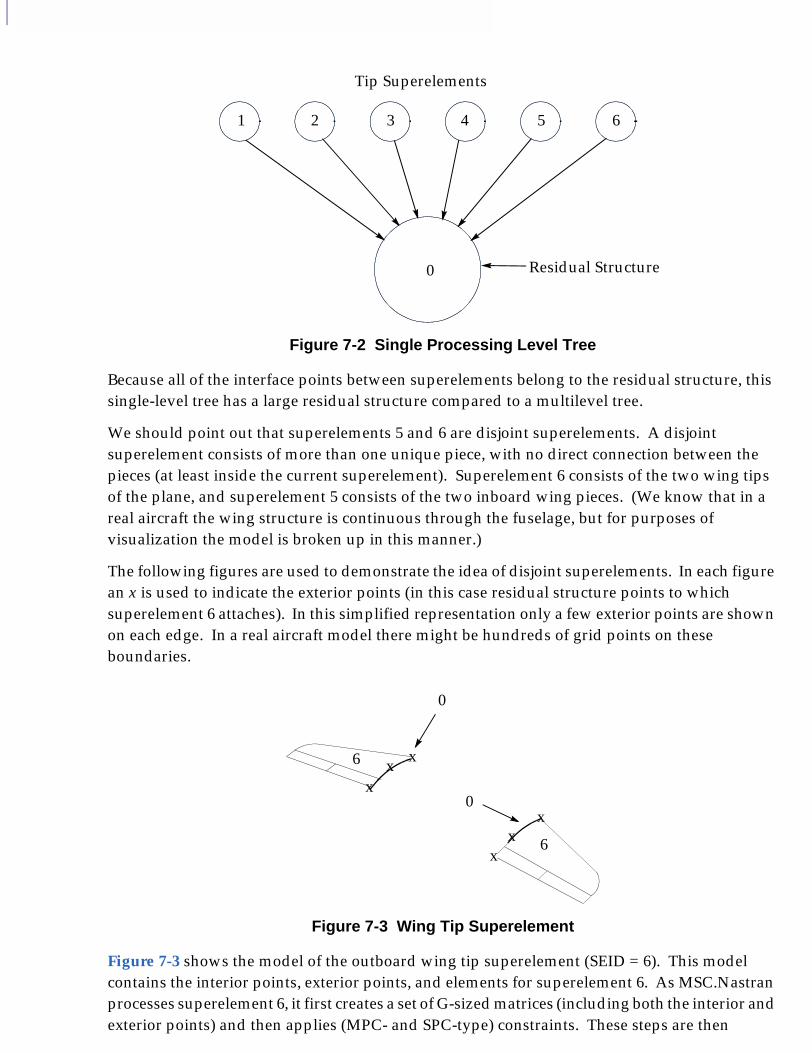
Figure 7-2 Single Processing Level Tree
Because all of the interface points between superelements belong to the residual structure, this single-level tree has a large residual structure compared to a multilevel tree.
We should point out that superelements 5 and 6 are disjoint superelements. A disjoint superelement consists of more than one unique piece, with no direct connection between the pieces (at least inside the current superelement). Superelement 6 consists of the two wing tips of the plane, and superelement 5 consists of the two inboard wing pieces. (We know that in a real aircraft the wing structure is continuous through the fuselage, but for purposes of visualization the model is broken up in this manner.)
The following figures are used to demonstrate the idea of disjoint superelements. In each figure an x is used to indicate the exterior points (in this case residual structure points to which superelement 6 attaches). In this simplified representation only a few exterior points are shown on each edge. In a real aircraft model there might be hundreds of grid points on these boundaries.
Figure 7-3 Wing Tip Superelement
Figure 7-3 shows the model of the outboard wing tip superelement (SEID = 6). This model contains the interior points, exterior points, and elements for superelement 6. As MSC.Nastran processes superelement 6, it first creates a set of G-sized matrices (including both the interior and exterior points) and then applies (MPC- and SPC-type) constraints. These steps are then
1 2 3 4 5 6
0 Residual Structure
Tip Superelements
0
0
6
6
xxx
xx
x
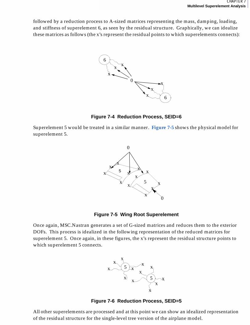
1CHAPTER 7Multilevel Superelement Analysis
followed by a reduction process to A-sized matrices representing the mass, damping, loading, and stiffness of superelement 6, as seen by the residual structure. Graphically, we can idealize these matrices as follows (the x’s represent the residual points to which superelements connects):
Figure 7-4 Reduction Process, SEID=6
Superelement 5 would be treated in a similar manner. Figure 7-5 shows the physical model for superelement 5.
Figure 7-5 Wing Root Superelement
Once again, MSC.Nastran generates a set of G-sized matrices and reduces them to the exterior DOFs. This process is idealized in the following representation of the reduced matrices for superelement 5. Once again, in these figures, the x’s represent the residual structure points to which superelement 5 connects.
Figure 7-6 Reduction Process, SEID=5
All other superelements are processed and at this point we can show an idealized representation of the residual structure for the single-level tree version of the airplane model.
0
6
6
xxx
xx
x
0
0
5
5x
xx
xx
x xx
x xx
x
5
5x
xx
xx
x xx
x xx
x
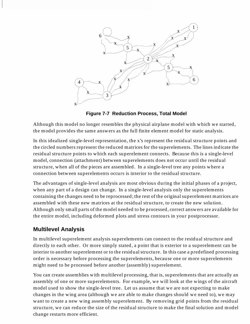
Figure 7-7 Reduction Process, Total Model
Although this model no longer resembles the physical airplane model with which we started, the model provides the same answers as the full finite element model for static analysis.
In this idealized single-level representation, the x’s represent the residual structure points and the circled numbers represent the reduced matrices for the superelements. The lines indicate the residual structure points to which each superelement connects. Because this is a single-level model, connection (attachment) between superelements does not occur until the residual structure, when all of the pieces are assembled. In a single-level tree any points where a connection between superelements occurs is interior to the residual structure.
The advantages of single-level analysis are most obvious during the initial phases of a project, when any part of a design can change. In a single-level analysis only the superelements containing the changes need to be reprocessed; the rest of the original superelement matrices are assembled with these new matrices at the residual structure, to create the new solution. Although only small parts of the model needed to be processed, correct answers are available for the entire model, including deformed plots and stress contours in your postprocessor.
Multilevel Analysis
In multilevel superelement analysis superelements can connect to the residual structure and directly to each other. Or more simply stated, a point that is exterior to a superelement can be interior to another superelement or to the residual structure. In this case a predefined processing order is necessary before processing the superelements, because one or more superelements might need to be processed before another (assembly) superelement.
You can create assemblies with multilevel processing, that is, superelements that are actually an assembly of one or more superelements. For example, we will look at the wings of the aircraft model used to show the single-level tree. Let us assume that we are not expecting to make changes in the wing area (although we are able to make changes should we need to), we may want to create a new wing assembly superelement. By removing grid points from the residual structure, we can reduce the size of the residual structure to make the final solution and model change restarts more efficient.
1
6
5
2
5
6
3
4
xx
x
xx
x
xx
xx
xx
x
xx
x
x
x
x
x
xx
x

1CHAPTER 7Multilevel Superelement Analysis
Sample of Multilevel Analysis, Example 1
For this case we will create a new collector superelement, which we will call superelement 56 (this number was chosen to imply that we have combined superelements 5 and 6 to create this assembly-any unused number could have been used). We will create this new collector by placing the grid points that lie on the boundary between superelements 5 and 6 into the new superelement (56). It is also advisable (mandatory, if PARTs are used) to define the processing tree-a topic that will be covered later in this section.
Figure 7-8 shows the original (single-level) model for the wings containing superelements 5 and 6 and the grid points connecting them.
Figure 7-8 Wing Model Single Level SE
To create a collector superelement, we will put the grid points lying on the interface between these superelements into superelement 56. (If PARTs are used, you can also define collector superelement 56 in the processing tree). This new definition of superelements is shown in Figure 7-9.
Figure 7-9 Wing Model, Multilevel Collector SEID=56
0
0
65
5
6
0
65
5
656
56
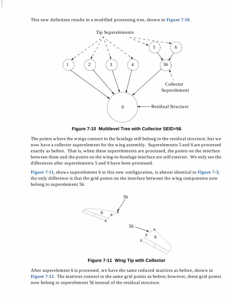
This new definition results in a modified processing tree, shown in Figure 7-10.
Figure 7-10 Multilevel Tree with Collector SEID=56
The points where the wings connect to the fuselage still belong to the residual structure, but we now have a collector superelement for the wing assembly. Superelements 5 and 6 are processed exactly as before. That is, when these superelements are processed, the points on the interface between them and the points on the wing-to-fuselage interface are still exterior. We only see the differences after superelements 5 and 6 have been processed.
Figure 7-11, shows superelement 6 in this new configuration, is almost identical to Figure 7-3; the only difference is that the grid points on the interface between the wing components now belong to superelement 56.
Figure 7-11 Wing Tip with Collector
After superelement 6 is processed, we have the same reduced matrices as before, shown in Figure 7-12. The matrices connect to the same grid points as before; however, these grid points now belong to superelement 56 instead of the residual structure.
65
1 2 3 4
0 Residual Structure
56
CollectorSuperelement
Tip Superelements
6
6
xxx
xx
x56
56
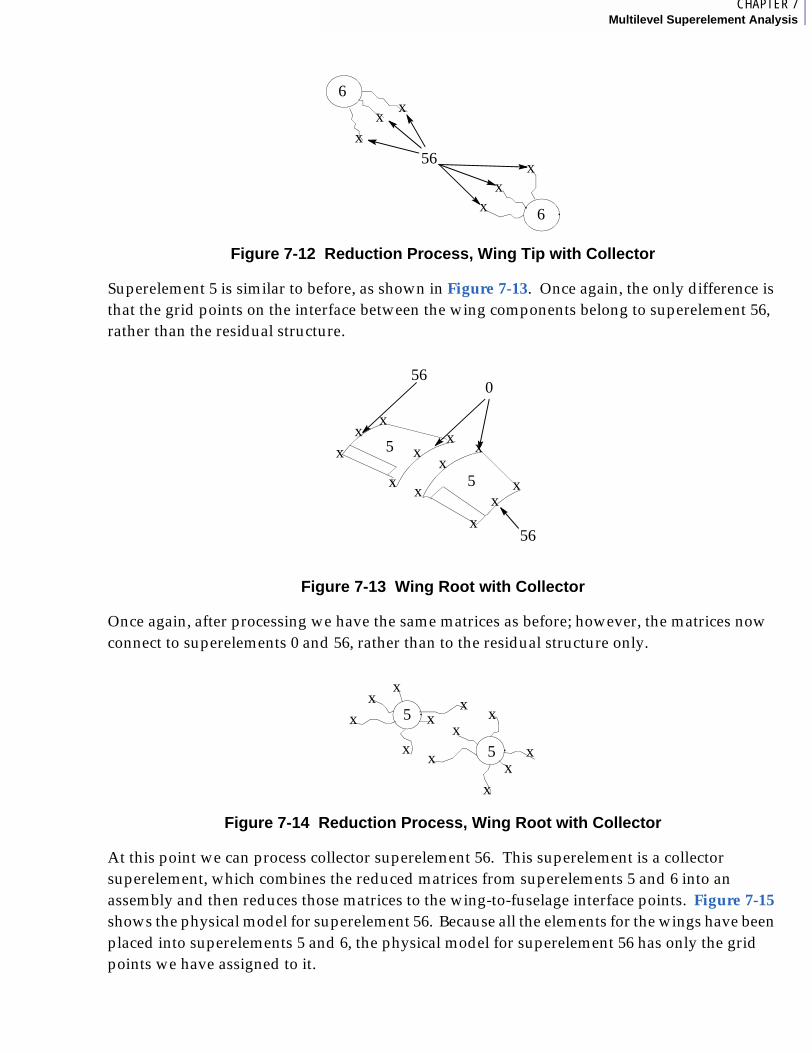
1CHAPTER 7Multilevel Superelement Analysis
Figure 7-12 Reduction Process, Wing Tip with Collector
Superelement 5 is similar to before, as shown in Figure 7-13. Once again, the only difference is that the grid points on the interface between the wing components belong to superelement 56, rather than the residual structure.
Figure 7-13 Wing Root with Collector
Once again, after processing we have the same matrices as before; however, the matrices now connect to superelements 0 and 56, rather than to the residual structure only.
Figure 7-14 Reduction Process, Wing Root with Collector
At this point we can process collector superelement 56. This superelement is a collector superelement, which combines the reduced matrices from superelements 5 and 6 into an assembly and then reduces those matrices to the wing-to-fuselage interface points. Figure 7-15 shows the physical model for superelement 56. Because all the elements for the wings have been placed into superelements 5 and 6, the physical model for superelement 56 has only the grid points we have assigned to it.
6
6
xxx
xx
x56
0
5
5x
xx
xx
x xx
x xx
x
56
56
5
5x
xx
xx
x xx
x xx
x
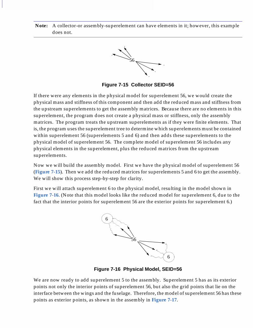
Figure 7-15 Collector SEID=56
If there were any elements in the physical model for superelement 56, we would create the physical mass and stiffness of this component and then add the reduced mass and stiffness from the upstream superelements to get the assembly matrices. Because there are no elements in this superelement, the program does not create a physical mass or stiffness, only the assembly matrices. The program treats the upstream superelements as if they were finite elements. That is, the program uses the superelement tree to determine which superelements must be contained within superelement 56 (superelements 5 and 6) and then adds these superelements to the physical model of superelement 56. The complete model of superelement 56 includes any physical elements in the superelement, plus the reduced matrices from the upstream superelements.
Now we will build the assembly model. First we have the physical model of superelement 56 (Figure 7-15). Then we add the reduced matrices for superelements 5 and 6 to get the assembly. We will show this process step-by-step for clarity.
First we will attach superelement 6 to the physical model, resulting in the model shown in Figure 7-16. (Note that this model looks like the reduced model for superelement 6, due to the fact that the interior points for superelement 56 are the exterior points for superelement 6.)
Figure 7-16 Physical Model, SEID=56
We are now ready to add superelement 5 to the assembly. Superelement 5 has as its exterior points not only the interior points of superelement 56, but also the grid points that lie on the interface between the wings and the fuselage. Therefore, the model of superelement 56 has these points as exterior points, as shown in the assembly in Figure 7-17.
Note: A collector-or assembly-superelement can have elements in it; however, this example does not.
56
..
.
.
..
6
6
56
..
.
.
..
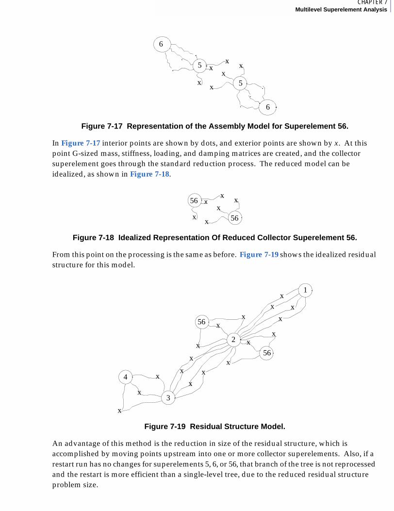
1CHAPTER 7Multilevel Superelement Analysis
Figure 7-17 Representation of the Assembly Model for Superelement 56.
In Figure 7-17 interior points are shown by dots, and exterior points are shown by x. At this point G-sized mass, stiffness, loading, and damping matrices are created, and the collector superelement goes through the standard reduction process. The reduced model can be idealized, as shown in Figure 7-18.
Figure 7-18 Idealized Representation Of Reduced Collector Superelement 56.
From this point on the processing is the same as before. Figure 7-19 shows the idealized residual structure for this model.
Figure 7-19 Residual Structure Model.
An advantage of this method is the reduction in size of the residual structure, which is accomplished by moving points upstream into one or more collector superelements. Also, if a restart run has no changes for superelements 5, 6, or 56, that branch of the tree is not reprocessed and the restart is more efficient than a single-level tree, due to the reduced residual structure problem size.
5
5x
xx x
x
x
6
6.
.
.
..
.
x
xx x
x
x 56
56
1
2
3
4
xx
xx
xx
x
xx
x
x
x
x
x
xx
x
56
56
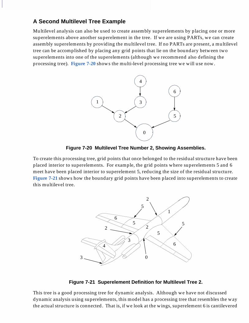
A Second Multilevel Tree Example
Multilevel analysis can also be used to create assembly superelements by placing one or more superelements above another superelement in the tree. If we are using PARTs, we can create assembly superelements by providing the multilevel tree. If no PARTs are present, a multilevel tree can be accomplished by placing any grid points that lie on the boundary between two superelements into one of the superelements (although we recommend also defining the processing tree). Figure 7-20 shows the multi-level processing tree we will use now.
Figure 7-20 Multilevel Tree Number 2, Showing Assemblies.
To create this processing tree, grid points that once belonged to the residual structure have been placed interior to superelements. For example, the grid points where superelements 5 and 6 meet have been placed interior to superelement 5, reducing the size of the residual structure. Figure 7-21 shows how the boundary grid points have been placed into superelements to create this multilevel tree.
Figure 7-21 Superelement Definition for Multilevel Tree 2.
This tree is a good processing tree for dynamic analysis. Although we have not discussed dynamic analysis using superelements, this model has a processing tree that resembles the way the actual structure is connected. That is, if we look at the wings, superelement 6 is cantilevered
0
6
5
4
3
2
1
2
03
1
25
63
4
52
65
5
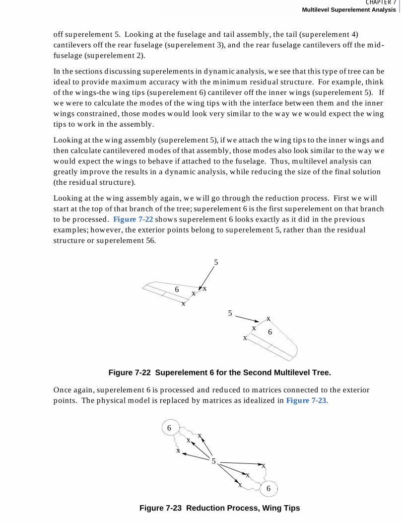
1CHAPTER 7Multilevel Superelement Analysis
off superelement 5. Looking at the fuselage and tail assembly, the tail (superelement 4) cantilevers off the rear fuselage (superelement 3), and the rear fuselage cantilevers off the mid-fuselage (superelement 2).
In the sections discussing superelements in dynamic analysis, we see that this type of tree can be ideal to provide maximum accuracy with the minimum residual structure. For example, think of the wings-the wing tips (superelement 6) cantilever off the inner wings (superelement 5). If we were to calculate the modes of the wing tips with the interface between them and the inner wings constrained, those modes would look very similar to the way we would expect the wing tips to work in the assembly.
Looking at the wing assembly (superelement 5), if we attach the wing tips to the inner wings and then calculate cantilevered modes of that assembly, those modes also look similar to the way we would expect the wings to behave if attached to the fuselage. Thus, multilevel analysis can greatly improve the results in a dynamic analysis, while reducing the size of the final solution (the residual structure).
Looking at the wing assembly again, we will go through the reduction process. First we will start at the top of that branch of the tree; superelement 6 is the first superelement on that branch to be processed. Figure 7-22 shows superelement 6 looks exactly as it did in the previous examples; however, the exterior points belong to superelement 5, rather than the residual structure or superelement 56.
Figure 7-22 Superelement 6 for the Second Multilevel Tree.
Once again, superelement 6 is processed and reduced to matrices connected to the exterior points. The physical model is replaced by matrices as idealized in Figure 7-23.
Figure 7-23 Reduction Process, Wing Tips
6
6
xxx
xx
x5
5
6
6
xxx
xx
x5
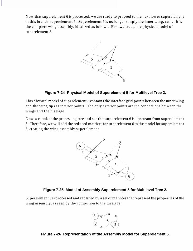
Now that superelement 6 is processed, we are ready to proceed to the next lower superelement in this branch-superelement 5. Superelement 5 is no longer simply the inner wing, rather it is the complete wing assembly, idealized as follows. First we create the physical model of superelement 5.
Figure 7-24 Physical Model of Superelement 5 for Multilevel Tree 2.
This physical model of superelement 5 contains the interface grid points between the inner wing and the wing tips as interior points. The only exterior points are the connections between the wings and the fuselage.
Now we look at the processing tree and see that superelement 6 is upstream from superelement 5. Therefore, we will add the reduced matrices for superelement 6 to the model for superelement 5, creating the wing assembly superelement.
Figure 7-25 Model of Assembly Superelement 5 for Multilevel Tree 2.
Superelement 5 is processed and replaced by a set of matrices that represent the properties of the wing assembly, as seen by the connection to the fuselage.
Figure 7-26 Representation of the Assembly Model for Superelement 5.
0
5
5x
xx x
x
x
5
5
0
5
5x
xx x
x
x
5
5
6
6
5
5x
xx x
x
x

1CHAPTER 7Multilevel Superelement Analysis
The tail-fuselage assembly is created in a similar manner. After all superelements are processed, the grid points at the connection between the fuselage and the wings are all that remain in the residual structure. These points are connected by matrices representing assembly superelements 2 and 5.
Figure 7-27 Residual Structure Model for Multilevel Sample 2.
As you can see, the residual structure has been reduced significantly from the single-level configuration. If multiple solutions are desired, the multilevel method is much more efficient.
A Third Example of A Multilevel Tree
Interestingly, the processing in multilevel analysis does not need to be physically intuitive; that is, the processing order can be varied to satisfy your particular interests or needs. For example, we will assume that the aircraft is far along in the design process (or perhaps we are updating an existing plane), and the only areas of the model we expect to change are the tail, middle fuselage, or forward fuselage. The following processing tree (Figure 7-28) allows us to use a smaller residual structure than the single-level tree, while being efficient for changes in superelements 1, 2, or 4. This fact does not mean that a change in superelements 3, 5, or 6 would be inefficient; however, the tree is optimized for changes to superelements 1, 2, or 4. Note that superelement 3 is above superelement 4 in the tree. Though we would not normally process these superelements in this way, we have placed superelement 4 immediately above the residual structure so that applying changes to this superelement will be efficient.
2x
x
x
xx
x
5
5
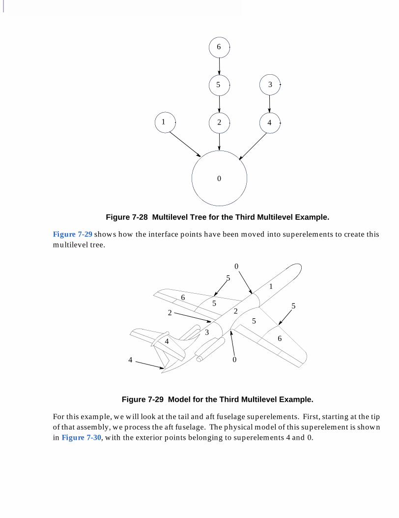
Figure 7-28 Multilevel Tree for the Third Multilevel Example.
Figure 7-29 shows how the interface points have been moved into superelements to create this multilevel tree.
Figure 7-29 Model for the Third Multilevel Example.
For this example, we will look at the tail and aft fuselage superelements. First, starting at the tip of that assembly, we process the aft fuselage. The physical model of this superelement is shown in Figure 7-30, with the exterior points belonging to superelements 4 and 0.
0
6
5
21
3
4
0
04
1
25
63
4
52
65
5
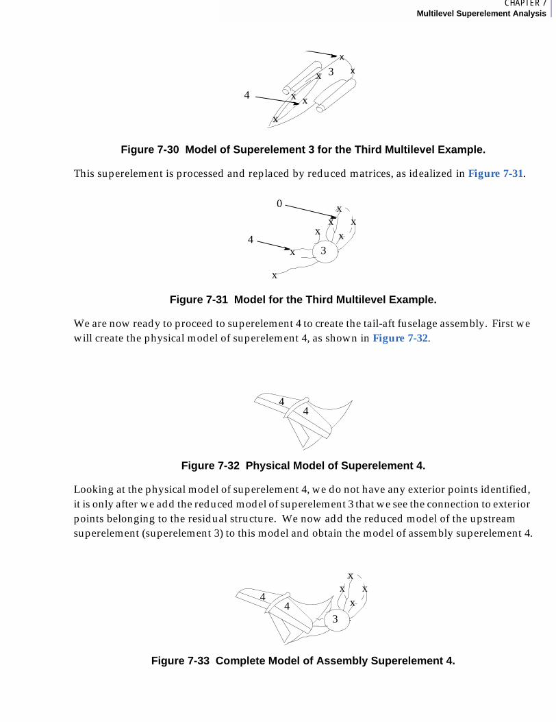
1CHAPTER 7Multilevel Superelement Analysis
Figure 7-30 Model of Superelement 3 for the Third Multilevel Example.
This superelement is processed and replaced by reduced matrices, as idealized in Figure 7-31.
Figure 7-31 Model for the Third Multilevel Example.
We are now ready to proceed to superelement 4 to create the tail-aft fuselage assembly. First we will create the physical model of superelement 4, as shown in Figure 7-32.
Figure 7-32 Physical Model of Superelement 4.
Looking at the physical model of superelement 4, we do not have any exterior points identified, it is only after we add the reduced model of superelement 3 that we see the connection to exterior points belonging to the residual structure. We now add the reduced model of the upstream superelement (superelement 3) to this model and obtain the model of assembly superelement 4.
Figure 7-33 Complete Model of Assembly Superelement 4.
4
3
x
x
xx
x
x
4
0
x
x
x
x
xxx
3
44
44
x
xxx
3

This superelement is processed and replaced by reduced matrices, which represent the properties of the aft assembly, as seen by the rest of the model.
Figure 7-34 Idealized Representation of the Aft Assembly.
After processing the other branches of the tree, the complete assembly will be created and solved at the residual structure.
As you can see, multilevel superelements give you complete control over the solution process. Single-level superelement analysis is simpler, but this analysis requires all superelements to connect only to the residual structure. With multilevel analysis you can create assemblies and reduce the size of the residual structure, resulting in increased efficiency for model changes.
x
xxx
4
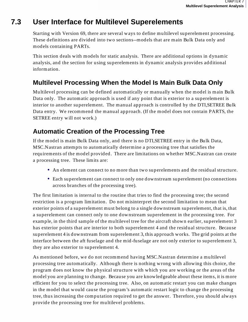
1CHAPTER 7Multilevel Superelement Analysis
7.3 User Interface for Multilevel SuperelementsStarting with Version 69, there are several ways to define multilevel superelement processing. These definitions are divided into two sections--models that are main Bulk Data only and models containing PARTs.
This section deals with models for static analysis. There are additional options in dynamic analysis, and the section for using superelements in dynamic analysis provides additional information.
Multilevel Processing When the Model Is Main Bulk Data OnlyMultilevel processing can be defined automatically or manually when the model is main Bulk Data only. The automatic approach is used if any point that is exterior to a superelement is interior to another superelement. The manual approach is controlled by the DTI,SETREE Bulk Data entry. We recommend the manual approach. (If the model does not contain PARTS, the SETREE entry will not work.)
Automatic Creation of the Processing TreeIf the model is main Bulk Data only, and there is no DTI,SETREE entry in the Bulk Data, MSC.Nastran attempts to automatically determine a processing tree that satisfies the requirements of the model provided. There are limitations on whether MSC.Nastran can create a processing tree. These limits are:
• An element can connect to no more than two superelements and the residual structure.
• Each superelement can connect to only one downstream superelement (no connections across branches of the processing tree).
The first limitation is internal to the routine that tries to find the processing tree; the second restriction is a program limitation. Do not misinterpret the second limitation to mean that exterior points of a superelement must belong to a single downstream superelement, that is, that a superelement can connect only to one downstream superelement in the processing tree. For example, in the third sample of the multilevel tree for the aircraft shown earlier, superelement 3 has exterior points that are interior to both superelement 4 and the residual structure. Because superelement 4 is downstream from superelement 3, this approach works. The grid points at the interface between the aft fuselage and the mid-fuselage are not only exterior to superelement 3, they are also exterior to superelement 4.
As mentioned before, we do not recommend having MSC.Nastran determine a multilevel processing tree automatically. Although there is nothing wrong with allowing this choice, the program does not know the physical structure with which you are working or the areas of the model you are planning to change. Because you are knowledgeable about these items, it is more efficient for you to select the processing tree. Also, on automatic restart you can make changes in the model that would cause the program’s automatic restart logic to change the processing tree, thus increasing the computation required to get the answer. Therefore, you should always provide the processing tree for multilevel problems.

There is a Case Control command that can be used to assist the automatic logic. This command is SEFINAL. The SEFINAL command is used to force the automatic process to place one or more superelements at the level immediately above the residual structure in the processing tree. If you use the automatic creation of the processing tree, you may want to use this command to select the superelement (or set of superelements) that will be at the lowest level above the residual. In this way, you can attempt to improve the restart efficiency when you are making changes.
Manual Definition of the Processing Tree for a Model Defined in the Main Bulk Data Section OnlyThere are two main Bulk Data entries that can be used to define the processing tree. One entry is DTI,SETREE. This entry can be used to manually define a multilevel processing tree for a model defined in the Main Bulk Data Section only. If the model contains PARTs, either the DTI,SETREE or SETREE entries are mandatory to obtain a multilevel tree.
In versions prior to Version 69, the DTI, SETREE was the only Bulk Data entry that could be used to define the multilevel tree. The SETREE entry was introduced in Version 69 to offer an alternative method.
With the DTI,SETREE entry you can specify the entire processing tree using one entry.
The DTI,SETREE is a table that you provide. The table is provided as record 1 (field 3 on the entry). After the record number, pairs of superelements are provided [seupi-sedowni] until the tree is defined. Continuation lines can be used.
The following example defines the tree shown in Figure 7-28.
DTI,SETREE,1,1,0,6,5,5,2,,2,0,3,4,4,0
Notice that the superelements are listed in upstream and downstream pairs, and the entire tree is given using one entry.
Multilevel Processing When the Model Uses PARTsIf the model includes PARTs, the SETREE or DTI,SETREE entries must be used if a multilevel tree is desired. Models containing PARTs are automatically treated as single-level, unless one of these entries appears in the Main Bulk Data Section. Otherwise, the SETREE and DTI,SETREE define a tree in the same manner as models defined in the Main Bulk Data Section only. Once again, these entries must be in the Main Bulk Data Section of the input file.
The SETREE entry actually provides a list of all superelements immediately upstream from a single superelement in the tree. One SETREE is required for each superelement that has any upstream connections.
1 2 3 4 5 6 7 8 9 10
DTI SETREE “1" SEUP1 SEDOWN1 SEUP2 SEDOWN2 SEUP3 SEDOWN3
SEUP4 SEDOWN4 SEUP5 SEDOWN5 -etc.-

1CHAPTER 7Multilevel Superelement Analysis
The following set of SETREE entries accomplishes the same tree as the above DTI,SETREE for Figure 7-28.
SETREE,0,1,2,4SETREE,2,5SETREE,5,6SETREE,4,3
In this set the first entry states that superelements 1, 2, and 4 are directly above the residual structure. The second entry states that superelement 5 is directly above superelement 2, etc.
Either the SETREE or the DTI,SETREE can be used, and if both entries are in the input file, the SETREE takes precedence. Also note that these entries must be in the Main Bulk Data Section if they are used. Verify that all superelements you want to include in the analysis are listed on the SETREE (or DTI,SETREE) entries, because superelements that are not listed are placed directly above the residual structure.
1 2 3 4 5 6 7 8 9 10
SETREE SEID SEUP1 SEUP2 SEUP3 SEUP4 SEUP5 SEUP6 SEUP7
SEUP8 SEUP9 -etc.-
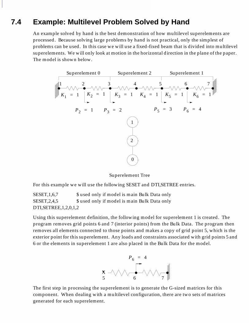
7.4 Example: Multilevel Problem Solved by HandAn example solved by hand is the best demonstration of how multilevel superelements are processed. Because solving large problems by hand is not practical, only the simplest of problems can be used. In this case we will use a fixed-fixed beam that is divided into multilevel superelements. We will only look at motion in the horizontal direction in the plane of the paper. The model is shown below.
For this example we will use the following SESET and DTI,SETREE entries.
SESET,1,6,7 $ used only if model is main Bulk Data onlySESET,2,4,5 $ used only if model is main Bulk Data onlyDTI,SETREE,1,2,0,1,2
Using this superelement definition, the following model for superelement 1 is created. The program removes grid points 6 and 7 (interior points) from the Bulk Data. The program then removes all elements connected to those points and makes a copy of grid point 5, which is the exterior point for this superelement. Any loads and constraints associated with grid points 5 and 6 or the elements in superelement 1 are also placed in the Bulk Data for the model.
The first step in processing the superelement is to generate the G-sized matrices for this component. When dealing with a multilevel configuration, there are two sets of matrices generated for each superelement.
1
2
0
Superelement 0 Superelement 2 Superelement 1
1 2 3 4 5 6 7
Superelement Tree
K1 1= K2 1= K3 1= K4 1= K5 1= K6 1=
P2 1= P3 2= P5 3= P6 4=
5 6 7X
P6 4=

1CHAPTER 7Multilevel Superelement Analysis
The first set of matrices created represent the physical properties of the superelement (plus any K2GG, M2GG, B2GG, or P2G matrices). The first set of matrices are G-sized and are defined by the letter J. For example, the physical stiffness matrix is called KJJ. The following stiffness and loading matrices are generated for superelement 1.
Eq. 7-1
The program will then create assembly G-sized matrices by combining these J matrices with the reduced matrices from upstream superelements. Because superelement 1 has no upstream superelements, the J and G matrices are the same. (Note that for this situation, where two matrices are identical, MSC.Nastran stores only one matrix in the database and will create a pointer for the second matrix, which points to the stored data. Therefore, the database files do not become excessively large.)
If there were any MPC-type relations (MPCs, RBE2, RBAR, etc), the program would apply and process these relations, and the G matrices would be reduced to N matrices.
The program then applies constraints to the matrices. For superelement 1, grid point 7 is constrained; thus, terms associated with this grid point are removed from the matrices to apply that constraint. After applying the constraints, the matrices are defined for the F set.
Eq. 7-2
At this point the static condensation is performed. The matrices are partitioned into A and O set DOFs and then transformed.
Eq. 7-3
Superelement 1 is now processed, and only the set of A sized matrices are required to continue the solution.
KJJ[ ]1. 1.– 0.1.– 2. 1.–
0. 1.– 1.
in term of
U5
U6
U7
=
PJ[ ]0.4.0.
=
KFF[ ] 1.0 1.–
1.– 2.0
KAA KAO
KOA KOO
= =
PF[ ] 0.4.
PA
PO
= =
GOA[ ] KOO[ ] 1–KOA[ ]– .5[ ]–= = 1.–[ ]⋅ .5[ ]=
KAA[ ] KAA[ ]= KOA[ ] TGOA[ ]+ 1.( )= .5( )– .5[ ]=
PA[ ] PA[ ]= GOA[ ] TPO[ ]+ 2.0[ ]=
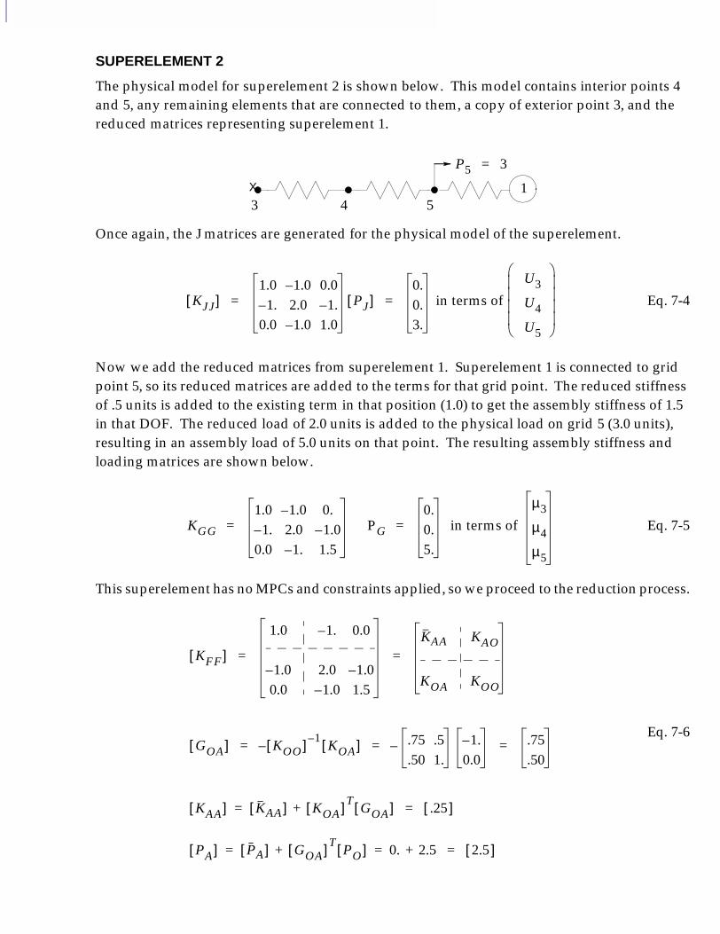
SUPERELEMENT 2
The physical model for superelement 2 is shown below. This model contains interior points 4 and 5, any remaining elements that are connected to them, a copy of exterior point 3, and the reduced matrices representing superelement 1.
Once again, the J matrices are generated for the physical model of the superelement.
Eq. 7-4
Now we add the reduced matrices from superelement 1. Superelement 1 is connected to grid point 5, so its reduced matrices are added to the terms for that grid point. The reduced stiffness of .5 units is added to the existing term in that position (1.0) to get the assembly stiffness of 1.5 in that DOF. The reduced load of 2.0 units is added to the physical load on grid 5 (3.0 units), resulting in an assembly load of 5.0 units on that point. The resulting assembly stiffness and loading matrices are shown below.
Eq. 7-5
This superelement has no MPCs and constraints applied, so we proceed to the reduction process.
Eq. 7-6
X
3 4 51
P5 3=
KJJ[ ]1.0 1.0– 0.0
1.– 2.0 1.–
0.0 1.0– 1.0
PJ[ ]0.0.3.
in terms of
U3
U4
U5
= =
KGG
1.0 1.0– 0.1.– 2.0 1.0–
0.0 1.– 1.5
PG
0.0.5.
in terms of
µ3
µ4
µ5
= =
KFF[ ]
1.0 1.– 0.0
1.0– 2.0 1.0–
0.0 1.0– 1.5
KAA KAO
KOA KOO
= =
GOA[ ] KOO[ ] 1–KOA[ ]– .75 .5
.50 1.1.–
0.0– .75
.50= = =
KAA[ ] KAA[ ]= KOA[ ] TGOA[ ]+ .25[ ]=
PA[ ] PA[ ]= GOA[ ] TPO[ ]+ 0.= 2.5+ 2.5[ ]=
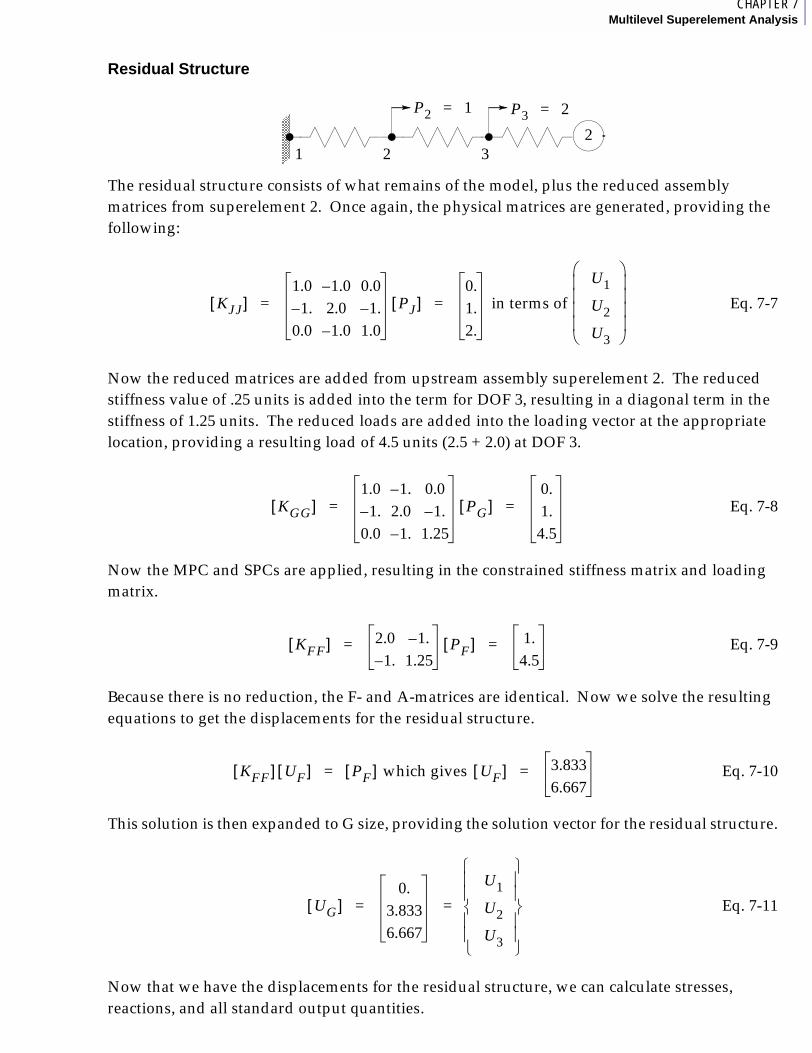
1CHAPTER 7Multilevel Superelement Analysis
Residual Structure
The residual structure consists of what remains of the model, plus the reduced assembly matrices from superelement 2. Once again, the physical matrices are generated, providing the following:
Eq. 7-7
Now the reduced matrices are added from upstream assembly superelement 2. The reduced stiffness value of .25 units is added into the term for DOF 3, resulting in a diagonal term in the stiffness of 1.25 units. The reduced loads are added into the loading vector at the appropriate location, providing a resulting load of 4.5 units (2.5 + 2.0) at DOF 3.
Eq. 7-8
Now the MPC and SPCs are applied, resulting in the constrained stiffness matrix and loading matrix.
Eq. 7-9
Because there is no reduction, the F- and A-matrices are identical. Now we solve the resulting equations to get the displacements for the residual structure.
Eq. 7-10
This solution is then expanded to G size, providing the solution vector for the residual structure.
Eq. 7-11
Now that we have the displacements for the residual structure, we can calculate stresses, reactions, and all standard output quantities.
1 2 32
P2 1= P3 2=
KJJ[ ]1.0 1.0– 0.0
1.– 2.0 1.–
0.0 1.0– 1.0
PJ[ ]0.1.2.
in terms of
U1
U2
U3
= =
KGG[ ]1.0 1.– 0.0
1.– 2.0 1.–
0.0 1.– 1.25
PG[ ]0.1.4.5
= =
KFF[ ] 2.0 1.–
1.– 1.25PF[ ] 1.
4.5= =
KFF[ ] UF[ ] PF[ ] which gives UF[ ] 3.8336.667
= =
UG[ ]0.
3.8336.667
U1
U2
U3
= =
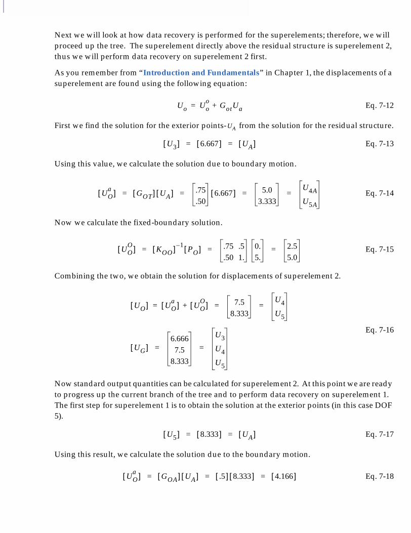
Next we will look at how data recovery is performed for the superelements; therefore, we will proceed up the tree. The superelement directly above the residual structure is superelement 2, thus we will perform data recovery on superelement 2 first.
As you remember from “Introduction and Fundamentals” in Chapter 1, the displacements of a superelement are found using the following equation:
Eq. 7-12
First we find the solution for the exterior points- from the solution for the residual structure.
Eq. 7-13
Using this value, we calculate the solution due to boundary motion.
Eq. 7-14
Now we calculate the fixed-boundary solution.
Eq. 7-15
Combining the two, we obtain the solution for displacements of superelement 2.
Eq. 7-16
Now standard output quantities can be calculated for superelement 2. At this point we are ready to progress up the current branch of the tree and to perform data recovery on superelement 1. The first step for superelement 1 is to obtain the solution at the exterior points (in this case DOF 5).
Eq. 7-17
Using this result, we calculate the solution due to the boundary motion.
Eq. 7-18
Uo Uoo
= GotUa+
UA
U3[ ] 6.667[ ] UA[ ]= =
UOa[ ] GOT[ ] UA[ ] .75
.506.667[ ] 5.0
3.333
U4A
U5A
= = = =
UOO[ ] KOO[ ] 1–
PO[ ] .75 .5.50 1.
0.5.
2.55.0
= = =
UO[ ] UOa[ ]= UO
O[ ]+ 7.58.333
U4
U5
= =
UG[ ]6.6667.5
8.333
U3
U4
U5
= =
U5[ ] 8.333[ ] UA[ ]= =
UOa[ ] GOA[ ] UA[ ] .5[ ] 8.333[ ] 4.166[ ]= = =

1CHAPTER 7Multilevel Superelement Analysis
Finally, we calculate the fixed boundary solution. Then we combine this result with the solution due to the boundary motion to get the displacements for superelement 1.
Eq. 7-19
For comparison, if we solve this problem as a residual structure only model, we get
Eq. 7-20
which gives
Eq. 7-21
The two approaches give identical answers, verifying that, for statics, using superelements for the solution does not introduce any approximation.
UOO[ ] KOO[ ] 1–
PO[ ] .5[ ] 4.0[ ] 2.0[ ]= = =
UO[ ] UOa[ ]= UO
O[ ]+ 4.166[ ]= 2.0[ ]+ 6.166[ ] U6[ ]= =
UG[ ]8.3336.1660.0
U5
U6
U7
= =
KFF[ ] UF{ } PF{ }
2. 1.– 0. 0. 0.1.– 2. 1.– 0. 0.
0. 1.– 2. 1.– 0.0. 0. 1.– 2. 1.–
0. 0. 0. 1.– 1.
U2
U3
U4
U5
U6
1.2.0.3.4.
= = =
U2
U3
U4
U5
U6
3.8336.6677.5
8.3336.166
=
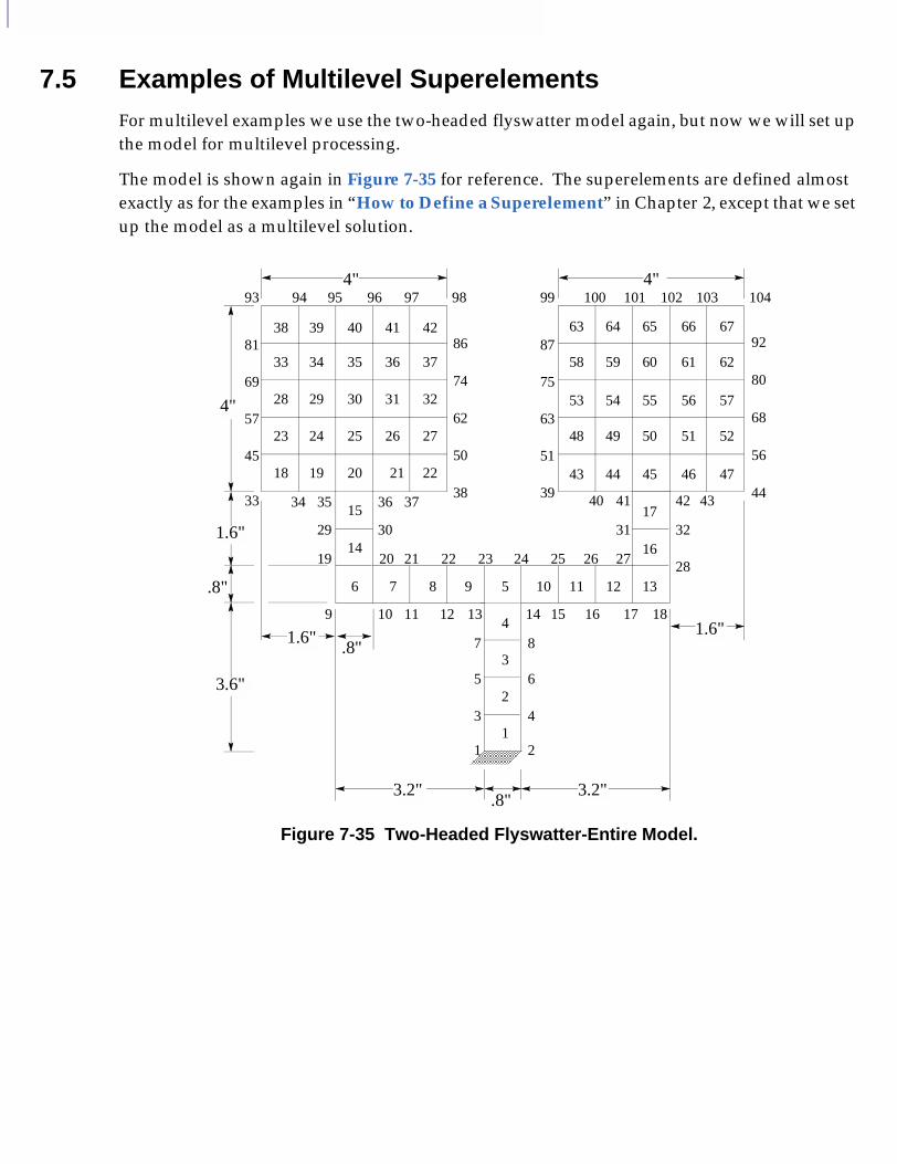
7.5 Examples of Multilevel SuperelementsFor multilevel examples we use the two-headed flyswatter model again, but now we will set up the model for multilevel processing.
The model is shown again in Figure 7-35 for reference. The superelements are defined almost exactly as for the examples in “How to Define a Superelement” in Chapter 2, except that we set up the model as a multilevel solution.
Figure 7-35 Two-Headed Flyswatter-Entire Model.
4" 4"
4"
1.6"
1.6" 1.6".8"
.8"
.8"3.2" 3.2"
3.6"
93 94 95 96 97 98 99 100 101 102 103 104
38 39 40 41 42
33 34 35 36 37
28 29 30 31 32
23 24 25 26 27
18 19 20 21 22
63 64 65 66 67
58 59 60 61 62
53 54 55 56 57
48 49 50 51 52
43 44 45
17
16
13
46 47
81
69
57
45
33
86
74
62
50
38
87
75
63
51
39
92
80
68
56
4434 35 36 37 40 41 42 43
15
14
6
9 10 11 12 13 14 15 16 17 18
19 20 21 22 23 24 25 26 27 28
29 30 31 32
1
2
3
4
5
6
7 8
1 2
3 4
5
7 8 9 10 11 12
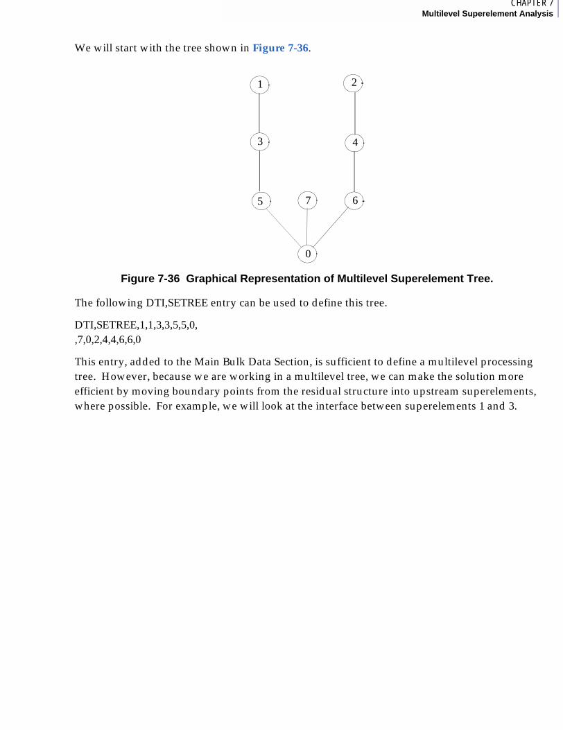
1CHAPTER 7Multilevel Superelement Analysis
We will start with the tree shown in Figure 7-36.
Figure 7-36 Graphical Representation of Multilevel Superelement Tree.
The following DTI,SETREE entry can be used to define this tree.
DTI,SETREE,1,1,3,3,5,5,0,,7,0,2,4,4,6,6,0
This entry, added to the Main Bulk Data Section, is sufficient to define a multilevel processing tree. However, because we are working in a multilevel tree, we can make the solution more efficient by moving boundary points from the residual structure into upstream superelements, where possible. For example, we will look at the interface between superelements 1 and 3.
1
3
5 7
0
6
4
2
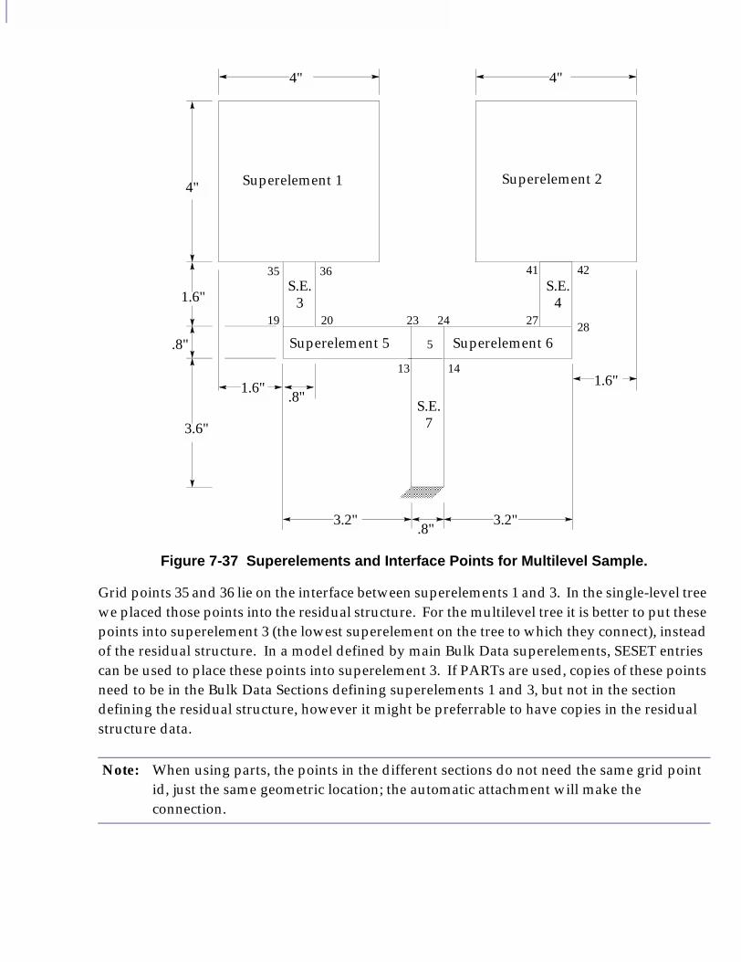
Figure 7-37 Superelements and Interface Points for Multilevel Sample.
Grid points 35 and 36 lie on the interface between superelements 1 and 3. In the single-level tree we placed those points into the residual structure. For the multilevel tree it is better to put these points into superelement 3 (the lowest superelement on the tree to which they connect), instead of the residual structure. In a model defined by main Bulk Data superelements, SESET entries can be used to place these points into superelement 3. If PARTs are used, copies of these points need to be in the Bulk Data Sections defining superelements 1 and 3, but not in the section defining the residual structure, however it might be preferrable to have copies in the residual structure data.
Note: When using parts, the points in the different sections do not need the same grid point id, just the same geometric location; the automatic attachment will make the connection.
4" 4"
4"
1.6"
1.6" 1.6".8"
.8"
.8"3.2" 3.2"
3.6"
35 36 41 42
13 14
19 20 23 24 2728
5
Superelement 1 Superelement 2
S.E.3
S.E.4
Superelement 5 Superelement 6
S.E.7
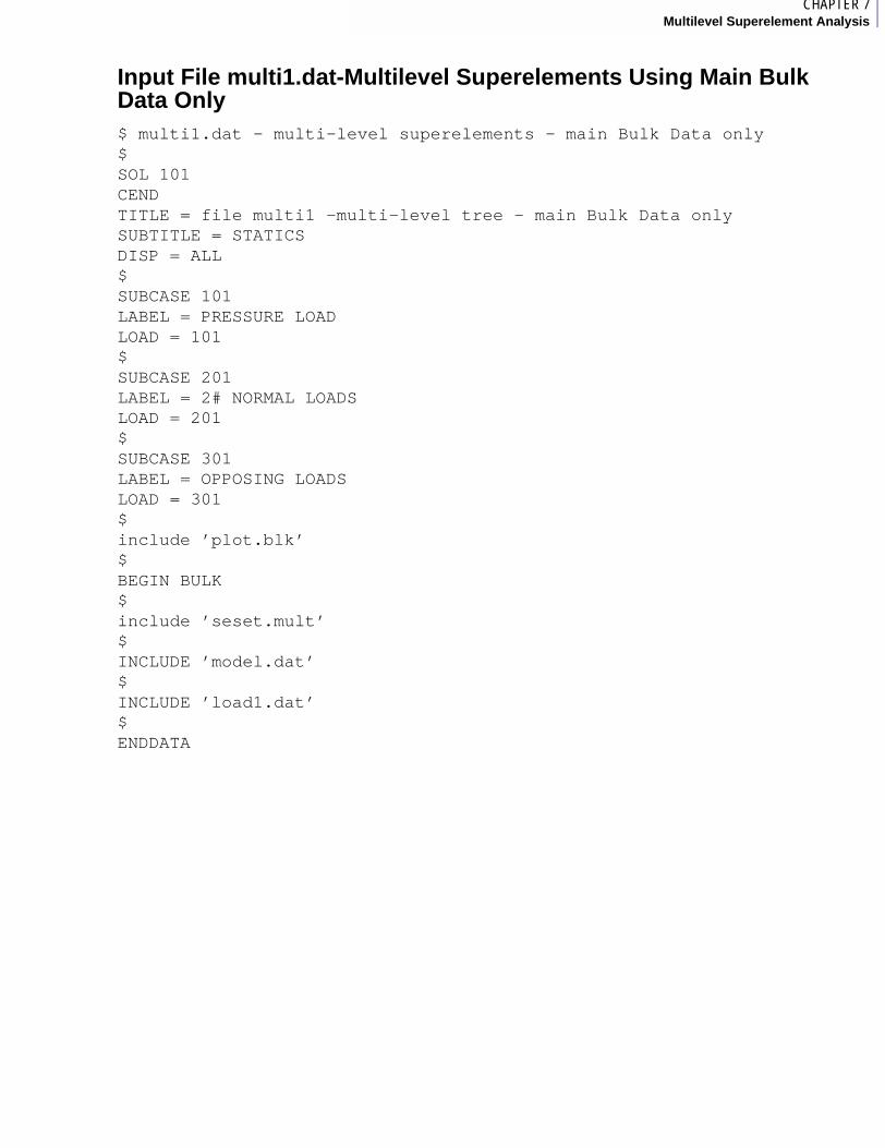
1CHAPTER 7Multilevel Superelement Analysis
Input File multi1.dat-Multilevel Superelements Using Main Bulk Data Only$ multi1.dat - multi-level superelements - main Bulk Data only$SOL 101 CENDTITLE = file multi1 -multi-level tree - main Bulk Data onlySUBTITLE = STATICS DISP = ALL$SUBCASE 101LABEL = PRESSURE LOADLOAD = 101$SUBCASE 201LABEL = 2# NORMAL LOADSLOAD = 201$SUBCASE 301LABEL = OPPOSING LOADSLOAD = 301$include ’plot.blk’$BEGIN BULK$include ’seset.mult’$INCLUDE ’model.dat’$INCLUDE ’load1.dat’$ENDDATA
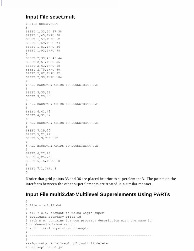
Input File seset.mult$ FILE SESET.MULT$SESET,1,33,34,37,38SESET,1,45,THRU,50SESET,1,57,THRU,62SESET,1,69,THRU,74SESET,1,81,THRU,86SESET,1,93,THRU,98$SESET,2,39,40,43,44SESET,2,51,THRU,56SESET,2,63,THRU,68SESET,2,75,THRU,80SESET,2,87,THRU,92SESET,2,99,THRU,104$$ ADD BOUNDARY GRIDS TO DOWNSTREAM S.E.$SESET,3,35,36SESET,3,29,30$$ ADD BOUNDARY GRIDS TO DOWNSTREAM S.E.$SESET,4,41,42SESET,4,31,32$$ ADD BOUNDARY GRIDS TO DOWNSTREAM S.E.$SESET,5,19,20SESET,5,21,22SESET,5,9,THRU,12$$ ADD BOUNDARY GRIDS TO DOWNSTREAM S.E.$SESET,6,27,28SESET,6,25,26SESET,6,15,THRU,18$SESET,7,1,THRU,8$
Notice that grid points 35 and 36 are placed interior to superelement 3. The points on the interfaces between the other superelements are treated in a similar manner.
Input File multi2.dat-Multilevel Superelements Using PARTs$$ file - multi2.dat $ $ all 7 s.e. brought in using begin super$ duplicate boundary grids id$ each s.e. contains its own property description with the same id$ condensed subcase setup$ multi-level superelement sample $$ ----------------------------------------------------------------$assign output2=’allsep1.op2’,unit=12,deleteid allsep1 dat $ jml
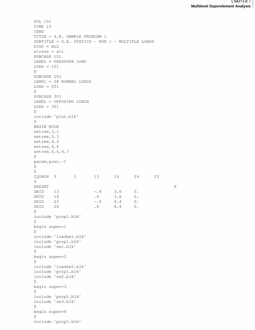
1CHAPTER 7Multilevel Superelement Analysis
SOL 101 TIME 15CENDTITLE = S.E. SAMPLE PROBLEM 1 SUBTITLE = S.E. STATICS - RUN 1 - MULTIPLE LOADSDISP = ALLstress = allSUBCASE 101LABEL = PRESSURE LOADLOAD = 101$SUBCASE 201LABEL = 2# NORMAL LOADSLOAD = 201$SUBCASE 301LABEL = OPPOSING LOADSLOAD = 301$include ’plot.blk’$BEGIN BULKsetree,3,1setree,5,3setree,4,2setree,6,4setree,0,5,6,7$param,post,-1$$ CQUAD4 5 1 13 14 24 23 $GRDSET 6 GRID 13 -.4 3.6 0. GRID 14 .4 3.6 0. GRID 23 -.4 4.4 0. GRID 24 .4 4.4 0. $include ’prop1.blk’$begin super=1$include ’loadse1.blk’include ’prop1.blk’include ’se1.blk’$begin super=2$ include ’loadse2.blk’include ’prop1.blk’include ’se2.blk’$begin super=3$ include ’prop1.blk’include ’se3.blk’$begin super=4$ include ’prop1.blk’

include ’se4.blk’$begin super=5$ include ’prop1.blk’include ’se5.blk’$begin super=6$ include ’prop1.blk’include ’se6.blk’$begin super=7$ include ’prop1.blk’include ’se7.blk’$enddata
The differences between multi2.dat and single2.dat are in the Main Bulk Data Section. These differences are: The SETREE entries are added to define the multilevel tree, and the interface points between the PARTs are not included in the Main Bulk Data Section and are, therefore, not residual structure points.
MSC.Nastran Assembly Modeling User’s Guide
CHAPTER
8 Output in Superelement Static Analysis
■ Sorted Bulk Data for PARTs
■ Boundary Grid Search Output for PARTs
■ Superelement Definition Table

8.1 Sorted Bulk Data for PARTsWhen superelements are used in static analysis, there are changes and additions to the standard output. First, the Bulk Data can be listed as a series of sections. If PARTs are used, the output has the sorted Bulk Data listing for the Main Bulk Data Section, followed by the section for each PART in the order in which they occur in the input file. Each set of output is labeled S O R T E D B U L K D A T A E C H O. The sorted data for the PARTs contains the PART number on this line. For example, each page containing sorted Bulk Data for PART 1 begins with:
S O R T E D B U L K D A T A E C H O SUPER = 1
The sorted data for the main Bulk Data from the input file inrel2.dat is:
Any entries occurring in the Main Bulk Data Section (that is, between BEGIN BULK and the first BEGIN SUPER or the ENDDATA, if no BEGIN SUPER is used) appear in this section. The INPUT BULK DATA COUNT is the total number of lines in the current section of the input file, including blank lines and comments.
INPUT BULK DATA CARD COUNT = 25 FILE INREL2.DAT - INERTIA RELIEF USING PARTS JULY 22, 2001 MSC.Nastran 7/22/01 PAGE 5 REFERENCE POINT IS POINT 13 IN RESIDUAL S O R T E D B U L K D A T A E C H O CARD COUNT . 1 .. 2 .. 3 .. 4 .. 5 .. 6 .. 7 .. 8 .. 9 .. 10 . 1- CQUAD4 5 1 13 14 24 23 2- GRID 13 -.4 3.6 0. 3- GRID 14 .4 3.6 0. 4- GRID 23 -.4 4.4 0. 5- GRID 24 .4 4.4 0. 6- MAT1 1 30.+6 .3 .283 7- PARAM AUTOSPC YES 8- PARAM INREL -1 9- PARAM POST -1 10- PARAM WTMASS .00259 11- PSHELL 1 1 .05 1 1 12- SUPORT 13 123456 ENDDATA
TOTAL COUNT= 13
Note: The total number for the Main Bulk Data Section in this model is 25, while the total count for the S O R T E D B U L K D A T A E C H O is only 13. The first number is the total number of entries, including blank lines and comments, and the total count after the sorted listing is the number of actual input lines used
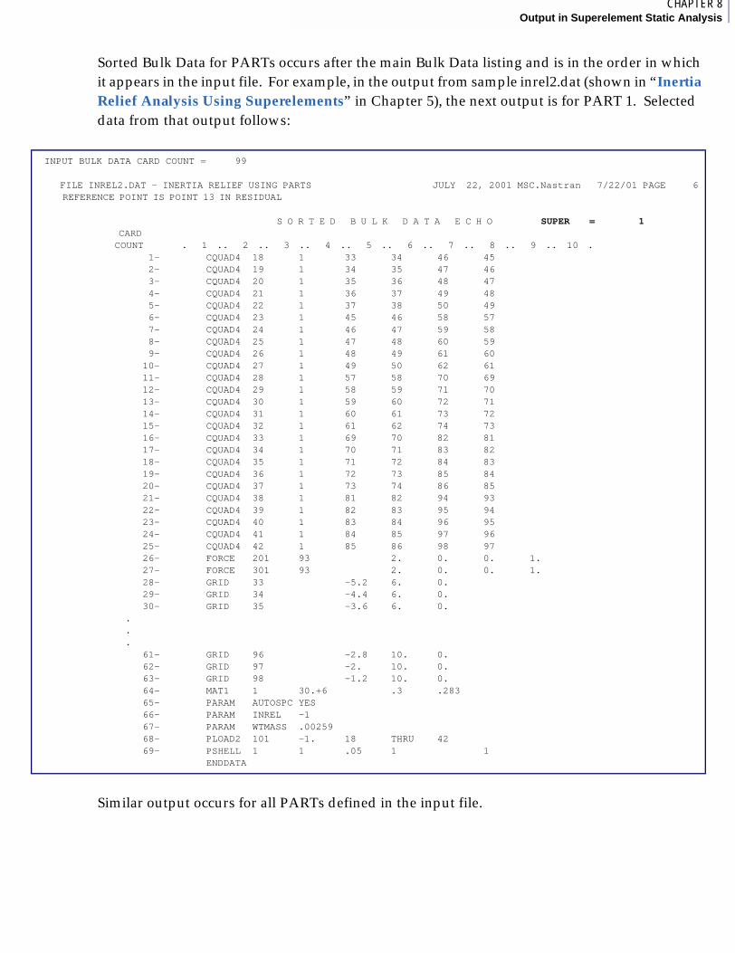
1CHAPTER 8Output in Superelement Static Analysis
Sorted Bulk Data for PARTs occurs after the main Bulk Data listing and is in the order in which it appears in the input file. For example, in the output from sample inrel2.dat (shown in “Inertia Relief Analysis Using Superelements” in Chapter 5), the next output is for PART 1. Selected data from that output follows:
Similar output occurs for all PARTs defined in the input file.
INPUT BULK DATA CARD COUNT = 99
FILE INREL2.DAT - INERTIA RELIEF USING PARTS JULY 22, 2001 MSC.Nastran 7/22/01 PAGE 6 REFERENCE POINT IS POINT 13 IN RESIDUAL S O R T E D B U L K D A T A E C H O SUPER = 1 CARD COUNT . 1 .. 2 .. 3 .. 4 .. 5 .. 6 .. 7 .. 8 .. 9 .. 10 . 1- CQUAD4 18 1 33 34 46 45 2- CQUAD4 19 1 34 35 47 46 3- CQUAD4 20 1 35 36 48 47 4- CQUAD4 21 1 36 37 49 48 5- CQUAD4 22 1 37 38 50 49 6- CQUAD4 23 1 45 46 58 57 7- CQUAD4 24 1 46 47 59 58 8- CQUAD4 25 1 47 48 60 59 9- CQUAD4 26 1 48 49 61 60 10- CQUAD4 27 1 49 50 62 61 11- CQUAD4 28 1 57 58 70 69 12- CQUAD4 29 1 58 59 71 70 13- CQUAD4 30 1 59 60 72 71 14- CQUAD4 31 1 60 61 73 72 15- CQUAD4 32 1 61 62 74 73 16- CQUAD4 33 1 69 70 82 81 17- CQUAD4 34 1 70 71 83 82 18- CQUAD4 35 1 71 72 84 83 19- CQUAD4 36 1 72 73 85 84 20- CQUAD4 37 1 73 74 86 85 21- CQUAD4 38 1 81 82 94 93 22- CQUAD4 39 1 82 83 95 94 23- CQUAD4 40 1 83 84 96 95 24- CQUAD4 41 1 84 85 97 96 25- CQUAD4 42 1 85 86 98 97 26- FORCE 201 93 2. 0. 0. 1. 27- FORCE 301 93 2. 0. 0. 1. 28- GRID 33 -5.2 6. 0. 29- GRID 34 -4.4 6. 0. 30- GRID 35 -3.6 6. 0. .
.
. 61- GRID 96 -2.8 10. 0. 62- GRID 97 -2. 10. 0. 63- GRID 98 -1.2 10. 0. 64- MAT1 1 30.+6 .3 .283 65- PARAM AUTOSPC YES 66- PARAM INREL -1 67- PARAM WTMASS .00259 68- PLOAD2 101 -1. 18 THRU 42 69- PSHELL 1 1 .05 1 1 ENDDATA
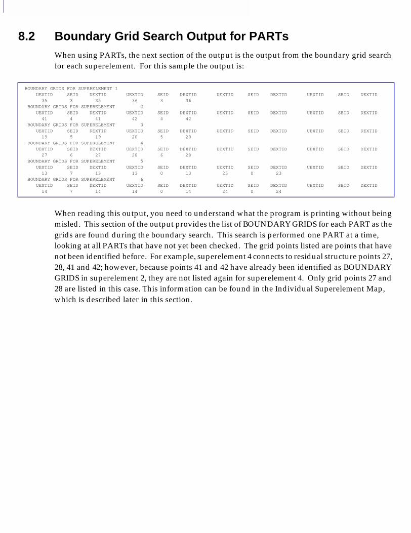
8.2 Boundary Grid Search Output for PARTsWhen using PARTs, the next section of the output is the output from the boundary grid search for each superelement. For this sample the output is:
When reading this output, you need to understand what the program is printing without being misled. This section of the output provides the list of BOUNDARY GRIDS for each PART as the grids are found during the boundary search. This search is performed one PART at a time, looking at all PARTs that have not yet been checked. The grid points listed are points that have not been identified before. For example, superelement 4 connects to residual structure points 27, 28, 41 and 42; however, because points 41 and 42 have already been identified as BOUNDARY GRIDS in superelement 2, they are not listed again for superelement 4. Only grid points 27 and 28 are listed in this case. This information can be found in the Individual Superelement Map, which is described later in this section.
BOUNDARY GRIDS FOR SUPERELEMENT 1 UEXTID SEID DEXTID UEXTID SEID DEXTID UEXTID SEID DEXTID UEXTID SEID DEXTID 35 3 35 36 3 36 BOUNDARY GRIDS FOR SUPERELEMENT 2 UEXTID SEID DEXTID UEXTID SEID DEXTID UEXTID SEID DEXTID UEXTID SEID DEXTID 41 4 41 42 4 42 BOUNDARY GRIDS FOR SUPERELEMENT 3 UEXTID SEID DEXTID UEXTID SEID DEXTID UEXTID SEID DEXTID UEXTID SEID DEXTID 19 5 19 20 5 20 BOUNDARY GRIDS FOR SUPERELEMENT 4 UEXTID SEID DEXTID UEXTID SEID DEXTID UEXTID SEID DEXTID UEXTID SEID DEXTID 27 6 27 28 6 28 BOUNDARY GRIDS FOR SUPERELEMENT 5 UEXTID SEID DEXTID UEXTID SEID DEXTID UEXTID SEID DEXTID UEXTID SEID DEXTID 13 7 13 13 0 13 23 0 23 BOUNDARY GRIDS FOR SUPERELEMENT 6 UEXTID SEID DEXTID UEXTID SEID DEXTID UEXTID SEID DEXTID UEXTID SEID DEXTID 14 7 14 14 0 14 24 0 24
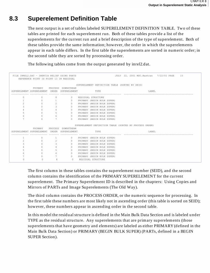
1CHAPTER 8Output in Superelement Static Analysis
8.3 Superelement Definition TableThe next output is a set of tables labeled SUPERELEMENT DEFINITION TABLE. Two of these tables are printed for each superelement run. Both of these tables provide a list of the superelements for the current run and a brief description of the type of superelement. Both of these tables provide the same information; however, the order in which the superelements appear in each table differs. In the first table the superelements are sorted in numeric order; in the second table they are sorted by processing order.
The following tables come from the output generated by inrel2.dat.
The first column in these tables contains the superelement number (SEID), and the second column contains the identification of the PRIMARY SUPERELEMENT for the current superelement. The Primary Superelement ID is described in the chapters: Using Copies and Mirrors of PARTs and Image Superelements (The Old Way).
The third column contains the PROCESS ORDER, or the numeric sequence for processing. In the first table these numbers are most likely not in ascending order (this table is sorted on SEID); however, these numbers appear in ascending order in the second table.
In this model the residual structure is defined in the Main Bulk Data Section and is labeled under TYPE as the residual structure. Any superelements that are primary superelements (those superelements that have geometry and elements) are labeled as either PRIMARY (defined in the Main Bulk Data Section) or PRIMARY (BEGIN BULK SUPER) (PARTs, defined in a BEGIN SUPER Section).
FILE INREL2.DAT - INERTIA RELIEF USING PARTS JULY 22, 2001 MSC.Nastran 7/22/01 PAGE 15 REFERENCE POINT IS POINT 13 IN RESIDUAL SUPERELEMENT DEFINITION TABLE (SORTED BY SEID) PRIMARY PROCESS DOWNSTREAMSUPERELEMENT SUPERELEMENT ORDER SUPERELEMENT TYPE LABEL------------ ------------ ------- ------------ ----------------------------- ------------------------------------------------ 0 0 8 0 RESIDUAL STRUCTURE 1 0 1 0 PRIMARY (BEGIN BULK SUPER) 2 0 2 0 PRIMARY (BEGIN BULK SUPER) 3 0 3 0 PRIMARY (BEGIN BULK SUPER) 4 0 4 0 PRIMARY (BEGIN BULK SUPER) 5 0 5 0 PRIMARY (BEGIN BULK SUPER) 6 0 6 0 PRIMARY (BEGIN BULK SUPER) 7 0 7 0 PRIMARY (BEGIN BULK SUPER)
SUPERELEMENT DEFINITION TABLE (SORTED BY PROCESS ORDER) PRIMARY PROCESS DOWNSTREAMSUPERELEMENT SUPERELEMENT ORDER SUPERELEMENT TYPE LABEL------------ ------------ ------- ------------ ----------------------------- ------------------------------------------------ 1 0 1 0 PRIMARY (BEGIN BULK SUPER) 2 0 2 0 PRIMARY (BEGIN BULK SUPER) 3 0 3 0 PRIMARY (BEGIN BULK SUPER) 4 0 4 0 PRIMARY (BEGIN BULK SUPER) 5 0 5 0 PRIMARY (BEGIN BULK SUPER) 6 0 6 0 PRIMARY (BEGIN BULK SUPER) 7 0 7 0 PRIMARY (BEGIN BULK SUPER) 0 0 8 0 RESIDUAL STRUCTURE

MSC.Nastran Superelements User’s Guide
CHAPTER
9 Introduction to Superelements in Dynamic Analysis
■ Description of Dynamic Reduction Procedures
■ Reduction Methods Used for Superelements
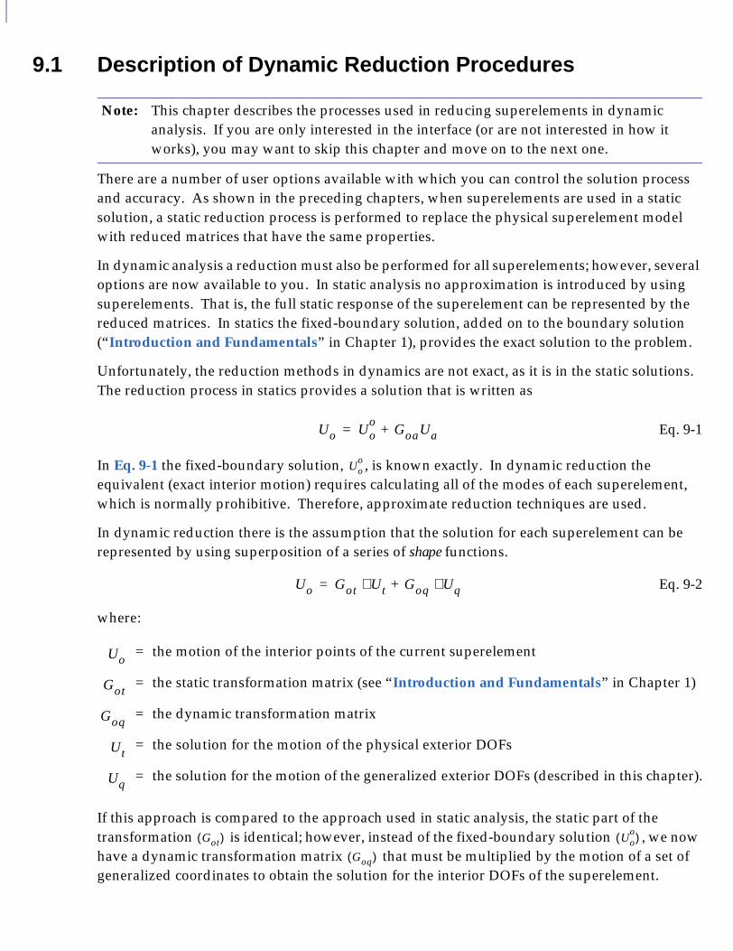
9.1 Description of Dynamic Reduction Procedures
There are a number of user options available with which you can control the solution process and accuracy. As shown in the preceding chapters, when superelements are used in a static solution, a static reduction process is performed to replace the physical superelement model with reduced matrices that have the same properties.
In dynamic analysis a reduction must also be performed for all superelements; however, several options are now available to you. In static analysis no approximation is introduced by using superelements. That is, the full static response of the superelement can be represented by the reduced matrices. In statics the fixed-boundary solution, added on to the boundary solution (“Introduction and Fundamentals” in Chapter 1), provides the exact solution to the problem.
Unfortunately, the reduction methods in dynamics are not exact, as it is in the static solutions. The reduction process in statics provides a solution that is written as
Eq. 9-1
In Eq. 9-1 the fixed-boundary solution, , is known exactly. In dynamic reduction the equivalent (exact interior motion) requires calculating all of the modes of each superelement, which is normally prohibitive. Therefore, approximate reduction techniques are used.
In dynamic reduction there is the assumption that the solution for each superelement can be represented by using superposition of a series of shape functions.
Eq. 9-2
where:
If this approach is compared to the approach used in static analysis, the static part of the transformation is identical; however, instead of the fixed-boundary solution , we now have a dynamic transformation matrix that must be multiplied by the motion of a set of generalized coordinates to obtain the solution for the interior DOFs of the superelement.
Note: This chapter describes the processes used in reducing superelements in dynamic analysis. If you are only interested in the interface (or are not interested in how it works), you may want to skip this chapter and move on to the next one.
= the motion of the interior points of the current superelement
= the static transformation matrix (see “Introduction and Fundamentals” in Chapter 1)
= the dynamic transformation matrix
= the solution for the motion of the physical exterior DOFs
= the solution for the motion of the generalized exterior DOFs (described in this chapter).
Uo Uoo
= GoaUa+
Uoo
Uo Got= Ut⋅ Goq+ Uq⋅
Uo
Got
Goq
Ut
Uq
Got( ) Uoo( )
Goq( )

1CHAPTER 9Introduction to Superelements in Dynamic Analysis
There are two classes of reduction used for superelements in dynamics: static reduction and dynamic reduction. Dynamic reduction is the more accurate approach for most problems, but dynamic reduction also requires more computational effort and some user judgement.
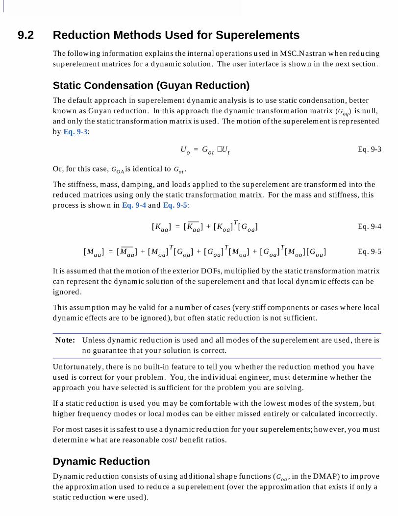
9.2 Reduction Methods Used for SuperelementsThe following information explains the internal operations used in MSC.Nastran when reducing superelement matrices for a dynamic solution. The user interface is shown in the next section.
Static Condensation (Guyan Reduction)The default approach in superelement dynamic analysis is to use static condensation, better known as Guyan reduction. In this approach the dynamic transformation matrix is null, and only the static transformation matrix is used. The motion of the superelement is represented by Eq. 9-3:
Eq. 9-3
Or, for this case, is identical to .
The stiffness, mass, damping, and loads applied to the superelement are transformed into the reduced matrices using only the static transformation matrix. For the mass and stiffness, this process is shown in Eq. 9-4 and Eq. 9-5:
Eq. 9-4
Eq. 9-5
It is assumed that the motion of the exterior DOFs, multiplied by the static transformation matrix can represent the dynamic solution of the superelement and that local dynamic effects can be ignored.
This assumption may be valid for a number of cases (very stiff components or cases where local dynamic effects are to be ignored), but often static reduction is not sufficient.
Unfortunately, there is no built-in feature to tell you whether the reduction method you have used is correct for your problem. You, the individual engineer, must determine whether the approach you have selected is sufficient for the problem you are solving.
If a static reduction is used you may be comfortable with the lowest modes of the system, but higher frequency modes or local modes can be either missed entirely or calculated incorrectly.
For most cases it is safest to use a dynamic reduction for your superelements; however, you must determine what are reasonable cost/benefit ratios.
Dynamic ReductionDynamic reduction consists of using additional shape functions ( , in the DMAP) to improve the approximation used to reduce a superelement (over the approximation that exists if only a static reduction were used).
Note: Unless dynamic reduction is used and all modes of the superelement are used, there is no guarantee that your solution is correct.
Goq( )
Uo Got= Ut⋅
GOA Got
Kaa[ ] Kaa[ ]= Koa[ ] TGoa[ ]+
Maa[ ] Maa[ ]= Moa[ ] TGoa[ ] Goa[ ] T
Moa[ ] Goa[ ] TMoo[ ] Goa[ ]+ + +
Goq

1CHAPTER 9Introduction to Superelements in Dynamic Analysis
For reference, we will look at conventional dynamic analysis. For many problems the mode shapes of a structure are used to transform the equations of motion into modal coordinates, thus simplifying the solution. If this approach is used, and all modes of a structure are used, no approximation occurs in this transformation.
Dynamic reduction of superelements is similar to the transformation of a structure into modal coordinates. However, the transformation involves the use of both static and dynamic shapes.
There are two types of dynamic reduction available when using superelements: Generalized Dynamic Reduction and Component Modal Synthesis. The following procedure is used by both of these methods.
As before, the static transformation matrix is generated. This operation is always performed, regardless of the reduction approach you use.
In dynamics a dynamic transformation can be performed in addition to the static transformation. A series of dynamic shape-functions ( , in DMAP) is found and used to dynamically transform the superelement properties to the exterior DOFs.
The shapes used to perform the dynamic reduction are chosen by the user; you can use either Generalized Dynamic Reduction or Component Modal Synthesis. With either approach the accuracy of the final solution depends on how many shape functions you use and how these shapes are calculated.
When either dynamic reduction approach is used, the program calculates dynamic shapes based on the boundary conditions you have selected.
At this point we must discuss the subsets of the A-set. The A-set in MSC.Nastran is the set containing all exterior DOFs for a superelement. When a superelement is processed, the component matrices are first generated for the G-set, then the matrices go through a series of processing steps until what remains is a set of reduced matrices that attach to the A-set DOFs. If the reduction is performed properly, these reduced matrices contain sufficient information to represent the dynamic behavior of the superelement.
The A-set is divided into several subsets for dynamic reduction. The following subsets of the A-set are used:
The A-set is divided into a number of subsets. These subsets determine whether an exterior DOF is held constrained during the calculation of the dynamic shape functions. Note that this has no affect on whether the points are constrained once the superelement has been processed.
For purposes of dynamic reduction, the T-set is divided into three subsets:
T Physical exterior DOF of the superelement
Q Generalized coordinates in the A-set
B Physical exterior DOF that are constrained during the calculation of the dynamic transformation vectors
Goq
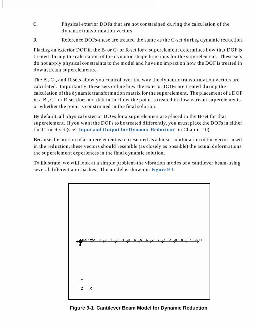
Placing an exterior DOF in the B- or C- or R-set for a superelement determines how that DOF is treated during the calculation of the dynamic shape functions for the superelement. These sets do not apply physical constraints to the model and have no impact on how the DOF is treated in downstream superelements.
The B-, C-, and R-sets allow you control over the way the dynamic transformation vectors are calculated. Importantly, these sets define how the exterior DOFs are treated during the calculation of the dynamic transformation matrix for the superelement. The placement of a DOF in a B-, C-, or R-set does not determine how the point is treated in downstream superelements or whether the point is constrained in the final solution.
By default, all physical exterior DOFs for a superelement are placed in the B-set for that superelement. If you want the DOFs to be treated differently, you must place the DOFs in either the C- or R-set (see “Input and Output for Dynamic Reduction” in Chapter 10).
Because the motion of a superelement is represented as a linear combination of the vectors used in the reduction, these vectors should resemble (as closely as possible) the actual deformations the superelement experiences in the final dynamic solution.
To illustrate, we will look at a simple problem-the vibration modes of a cantilever beam-using several different approaches. The model is shown in Figure 9-1.
Figure 9-1 Cantilever Beam Model for Dynamic Reduction
C Physical exterior DOFs that are not constrained during the calculation of the dynamic transformation vectors
R Reference DOFs-these are treated the same as the C-set during dynamic reduction.
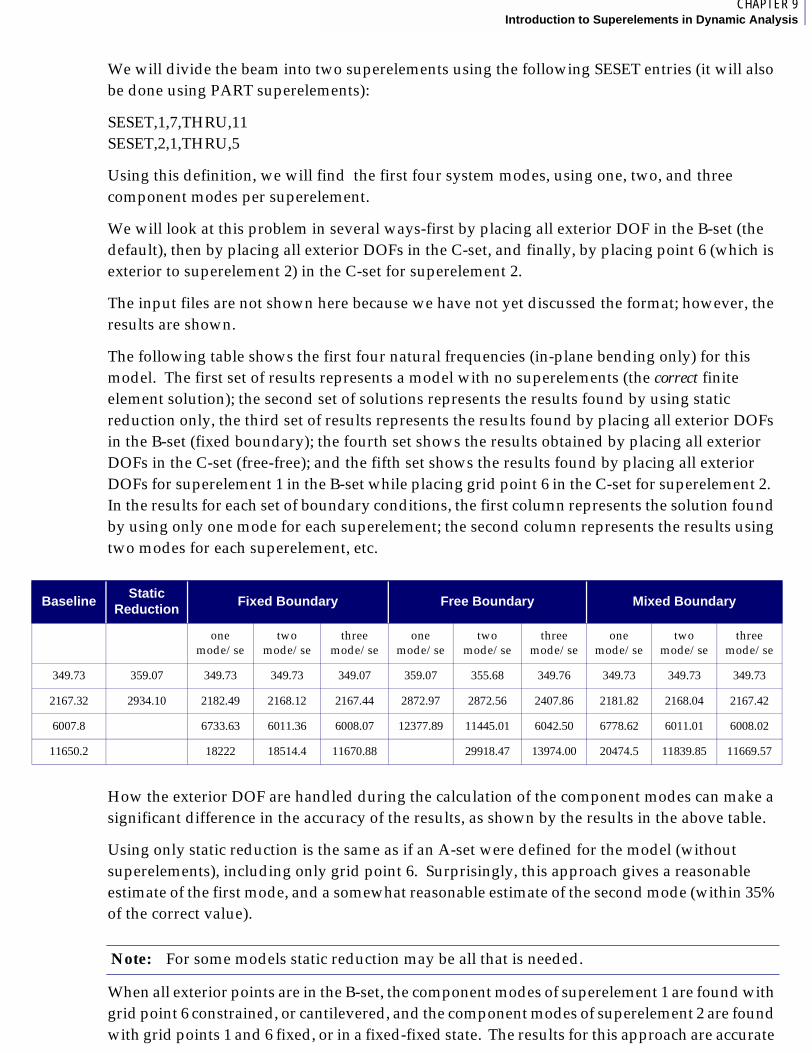
1CHAPTER 9Introduction to Superelements in Dynamic Analysis
We will divide the beam into two superelements using the following SESET entries (it will also be done using PART superelements):
SESET,1,7,THRU,11SESET,2,1,THRU,5
Using this definition, we will find the first four system modes, using one, two, and three component modes per superelement.
We will look at this problem in several ways-first by placing all exterior DOF in the B-set (the default), then by placing all exterior DOFs in the C-set, and finally, by placing point 6 (which is exterior to superelement 2) in the C-set for superelement 2.
The input files are not shown here because we have not yet discussed the format; however, the results are shown.
The following table shows the first four natural frequencies (in-plane bending only) for this model. The first set of results represents a model with no superelements (the correct finite element solution); the second set of solutions represents the results found by using static reduction only, the third set of results represents the results found by placing all exterior DOFs in the B-set (fixed boundary); the fourth set shows the results obtained by placing all exterior DOFs in the C-set (free-free); and the fifth set shows the results found by placing all exterior DOFs for superelement 1 in the B-set while placing grid point 6 in the C-set for superelement 2. In the results for each set of boundary conditions, the first column represents the solution found by using only one mode for each superelement; the second column represents the results using two modes for each superelement, etc.
How the exterior DOF are handled during the calculation of the component modes can make a significant difference in the accuracy of the results, as shown by the results in the above table.
Using only static reduction is the same as if an A-set were defined for the model (without superelements), including only grid point 6. Surprisingly, this approach gives a reasonable estimate of the first mode, and a somewhat reasonable estimate of the second mode (within 35% of the correct value).
When all exterior points are in the B-set, the component modes of superelement 1 are found with grid point 6 constrained, or cantilevered, and the component modes of superelement 2 are found with grid points 1 and 6 fixed, or in a fixed-fixed state. The results for this approach are accurate
BaselineStatic
ReductionFixed Boundary Free Boundary Mixed Boundary
one mode/se
two mode/se
three mode/se
one mode/se
two mode/se
three mode/se
one mode/se
two mode/se
three mode/se
349.73 359.07 349.73 349.73 349.07 359.07 355.68 349.76 349.73 349.73 349.73
2167.32 2934.10 2182.49 2168.12 2167.44 2872.97 2872.56 2407.86 2181.82 2168.04 2167.42
6007.8 6733.63 6011.36 6008.07 12377.89 11445.01 6042.50 6778.62 6011.01 6008.02
11650.2 18222 18514.4 11670.88 29918.47 13974.00 20474.5 11839.85 11669.57
Note: For some models static reduction may be all that is needed.
for this model. With only one mode for each superelement, the first two elastic modes of the model are predicted within 1%, and the third mode is predicted within 12%. When additional component modes are added, the results quickly converge to the correct solution. With three modes per superelement, the fourth system mode is predicted with an accuracy of better than 1%.
When all exterior points are in the C-set, the component modes of each superelement are found with no constraints applied on the exterior points, or (for this model) in the free-free state. For this version the first system mode is predicted well (within 2%) using only one mode per superelement. Notice that when using only one mode per superelement, the model finds only three system modes, which is explained later in this section. For this model predicting the second system mode using free-free CMS is difficult. Using three modes per superelement, the results for the second mode are only within 11% of the correct value, indicating how much impact the method used to handle the exterior points during CMS can have.
When the fourth approach is used, the component modes of superelement 1 are found with grid point 6 constrained (cantilevered), and the component modes of superelement 2 are found with grid point 1 fixed and no constraints on grid point 6 (cantilevered). These results are the best for all the methods shown.
Conclusion. We recommend dynamic reduction for almost all models using superelements in a dynamic solution. How you treat the exterior points during the dynamic reduction calculation is very important to the accuracy of your solution. We recommend calculating component modes (or GDR vectors) using the boundary condition that best approximates how you expect the component to behave when combined with the rest of the structure.
Fixed-Boundary Dynamic ReductionThe default method used in MSC.Nastran when performing a dynamic transformation of a superelement is the fixed-boundary approach, where all exterior DOF belong to the superelement’s B-set. If this approach is used, all exterior DOF are held fixed during the calculation of the dynamic transformation vectors. If component modal synthesis is used, the default method is better known as the Craig-Bampton approach (see “References” on page 225, which is the most commonly used approach.
Description of Methodology (Better Known as Craig-Bampton CMS). After applying any multipoint constraints and all physical constraints to the superelement, the component matrices have been reduced to the F-set. These (F-set) superelement matrices are partitioned into two sets of degrees-of-freedom (DOFs). The first set (the B-set) represents the boundary (exterior) points. The second set is the remaining interior DOFs (the O-set).
At this point a set of constraint modes is generated. Each constraint mode represents the motion of the superelement resulting from moving one boundary DOF 1.0 unit while holding the other boundary DOFs fixed. Therefore, there is one constraint mode for each boundary DOF. (These vectors are known as in MSC.Nastran.)GOT
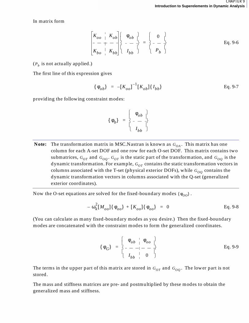
1CHAPTER 9Introduction to Superelements in Dynamic Analysis
In matrix form
Eq. 9-6
( is not actually applied.)
The first line of this expression gives
Eq. 9-7
providing the following constraint modes:
Now the O-set equations are solved for the fixed-boundary modes .
Eq. 9-8
(You can calculate as many fixed-boundary modes as you desire.) Then the fixed-boundary modes are concatenated with the constraint modes to form the generalized coordinates.
Eq. 9-9
The terms in the upper part of this matrix are stored in and . The lower part is not stored.
The mass and stiffness matrices are pre- and postmultiplied by these modes to obtain the generalized mass and stiffness.
Note: The transformation matrix in MSC.Nastran is known as . This matrix has one column for each A-set DOF and one row for each O-set DOF. This matrix contains two submatrices, and . is the static part of the transformation, and is the dynamic transformation. For example, contains the static transformation vectors in columns associated with the T-set (physical exterior DOFs), while contains the dynamic transformation vectors in columns associated with the Q-set (generalized exterior coordinates).
Koo Kob
Kbo Kbb
φob
Ibb 0
Pb
=
Pb
φob{ } Koo[ ] 1–Kob[ ] Ibb{ }–=
φb{ }φob
Ibb
=
GOA
GOT GOQ GOT GOQ
GOT
GOQ
φOO{ }
ωk2
Moo[ ] φoo{ }– Koo[ ] φoo{ }+ 0=
φG{ }φob φoo
Ibb 0
=
GOT GOQ
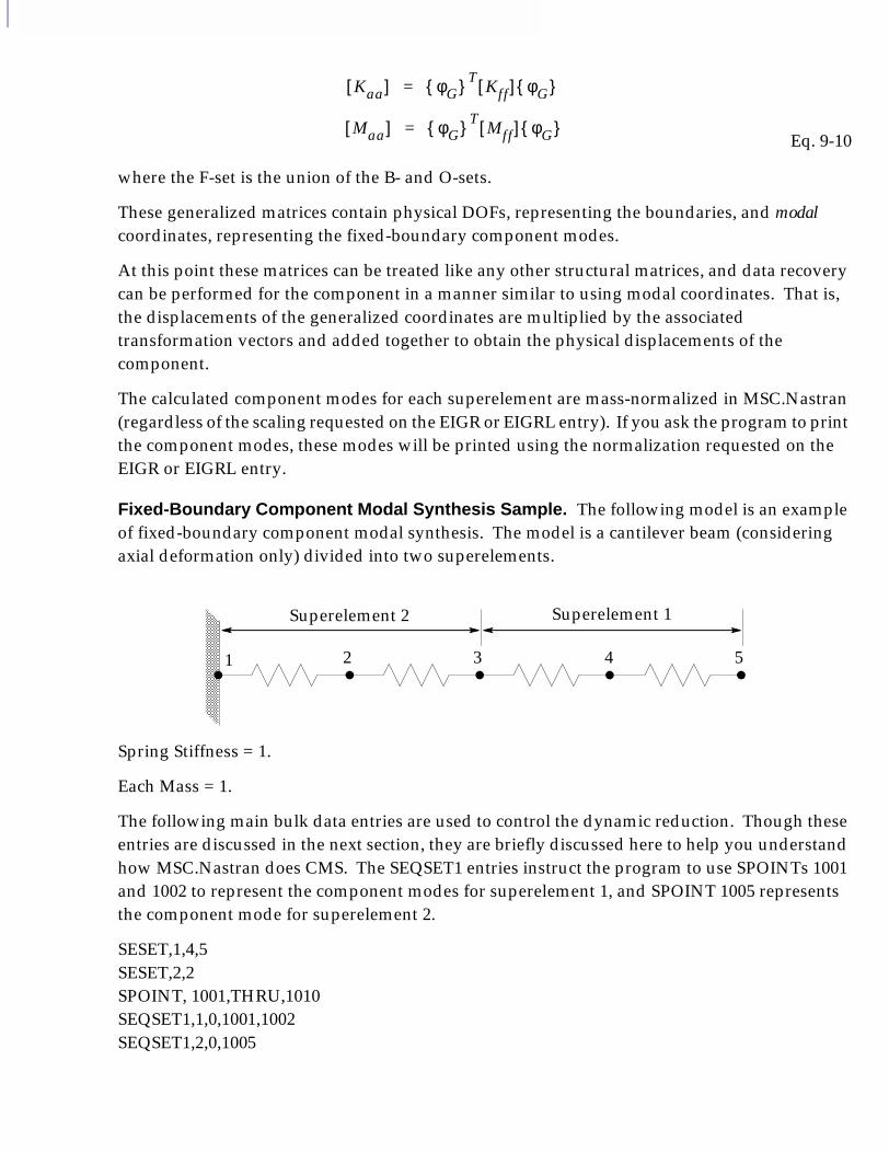
Eq. 9-10
where the F-set is the union of the B- and O-sets.
These generalized matrices contain physical DOFs, representing the boundaries, and modal coordinates, representing the fixed-boundary component modes.
At this point these matrices can be treated like any other structural matrices, and data recovery can be performed for the component in a manner similar to using modal coordinates. That is, the displacements of the generalized coordinates are multiplied by the associated transformation vectors and added together to obtain the physical displacements of the component.
The calculated component modes for each superelement are mass-normalized in MSC.Nastran (regardless of the scaling requested on the EIGR or EIGRL entry). If you ask the program to print the component modes, these modes will be printed using the normalization requested on the EIGR or EIGRL entry.
Fixed-Boundary Component Modal Synthesis Sample. The following model is an example of fixed-boundary component modal synthesis. The model is a cantilever beam (considering axial deformation only) divided into two superelements.
Spring Stiffness = 1.
Each Mass = 1.
The following main bulk data entries are used to control the dynamic reduction. Though these entries are discussed in the next section, they are briefly discussed here to help you understand how MSC.Nastran does CMS. The SEQSET1 entries instruct the program to use SPOINTs 1001 and 1002 to represent the component modes for superelement 1, and SPOINT 1005 represents the component mode for superelement 2.
SESET,1,4,5SESET,2,2SPOINT, 1001,THRU,1010SEQSET1,1,0,1001,1002SEQSET1,2,0,1005
Kaa[ ] φG{ } TKff[ ] φG{ }=
Maa[ ] φG{ } TMff[ ] φG{ }=
51 2 3 4
Superelement 2 Superelement 1
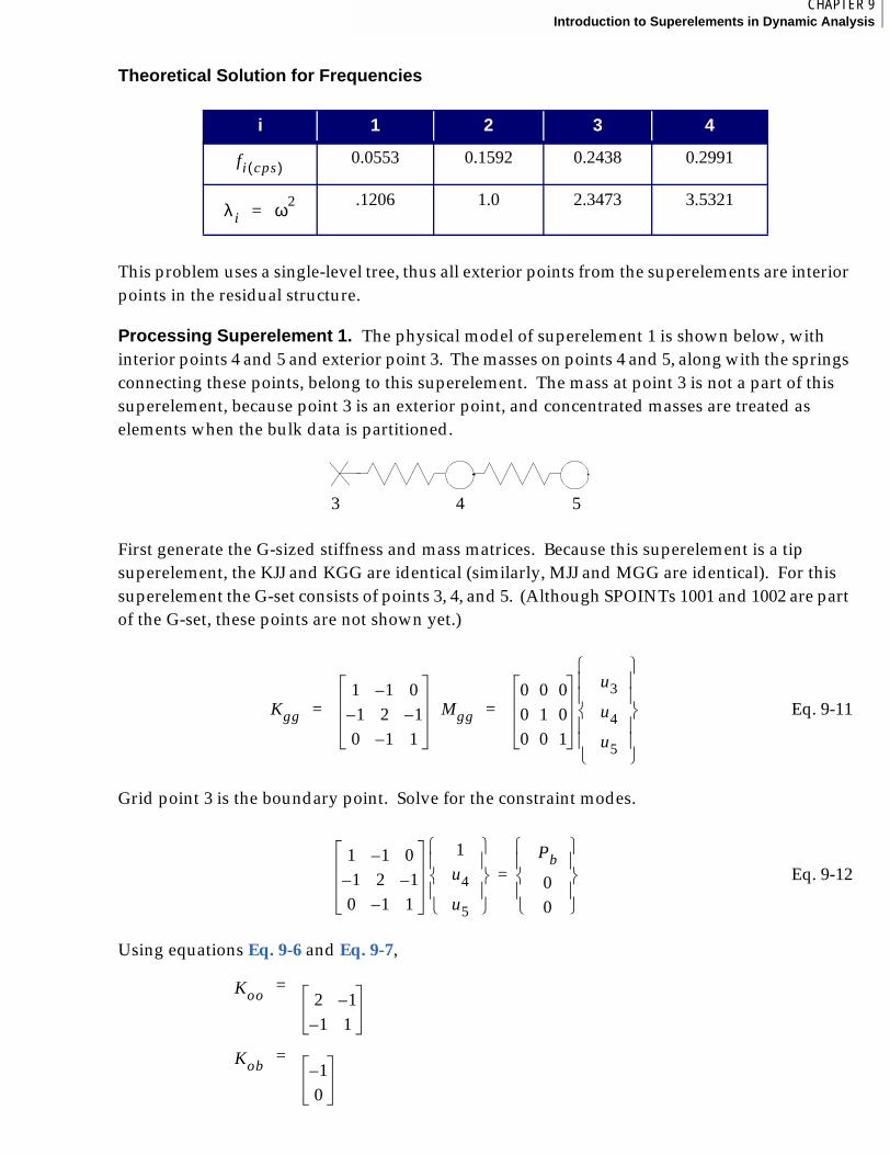
1CHAPTER 9Introduction to Superelements in Dynamic Analysis
Theoretical Solution for Frequencies
This problem uses a single-level tree, thus all exterior points from the superelements are interior points in the residual structure.
Processing Superelement 1. The physical model of superelement 1 is shown below, with interior points 4 and 5 and exterior point 3. The masses on points 4 and 5, along with the springs connecting these points, belong to this superelement. The mass at point 3 is not a part of this superelement, because point 3 is an exterior point, and concentrated masses are treated as elements when the bulk data is partitioned.
First generate the G-sized stiffness and mass matrices. Because this superelement is a tip superelement, the KJJ and KGG are identical (similarly, MJJ and MGG are identical). For this superelement the G-set consists of points 3, 4, and 5. (Although SPOINTs 1001 and 1002 are part of the G-set, these points are not shown yet.)
Eq. 9-11
Grid point 3 is the boundary point. Solve for the constraint modes.
Eq. 9-12
Using equations Eq. 9-6 and Eq. 9-7,
i 1 2 3 4
0.0553 0.1592 0.2438 0.2991
.1206 1.0 2.3473 3.5321
=
=
fi cps( )
λ i ω2=
3 4 5
Kgg
1 1– 01– 2 1–
0 1– 1
= Mgg
0 0 00 1 00 0 1
u3
u4
u5
=
1 1– 01– 2 1–
0 1– 1
1u4
u5 Pb
00
=
Koo 2 1–
1– 1
Kob 1–
0
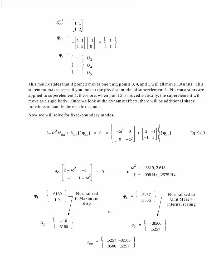
This matrix states that if point 3 moves one unit, points 3, 4, and 5 will all move 1.0 units. This statement makes sense if you look at the physical model of superelement 1. No constraints are applied to superelement 1; therefore, when point 3 is moved statically, the superelement will move as a rigid body. Once we look at the dynamic effects, there will be additional shape functions to handle the elastic response.
Now we will solve for fixed-boundary modes.
Eq. 9-13
=
=
=
Koo1–
1 11 2
φob 1 11 2
1–
0– 1
1
=
φb111
U3
U4
U5
ω2Moo– Koo+[ ] φoo{ } 0. ω2
– 0
0 ω2–
2 1–
1– 1+
φoo{ }= =
Normalized to Maximum
disp
Normalized to Unit Mass =
internal scaling
or
det 2 ω2– 1–
1– 1 ω2–
0=ω2 .3819, 2.618=
f .098 Hz, .2575 Hz=
φ1.5257.8506
=φ1.61801.0
=
φ21.0–
.6180
= φ2.8506–
.5257
=
φoo.5257 .8506–
.8506 .5257
=
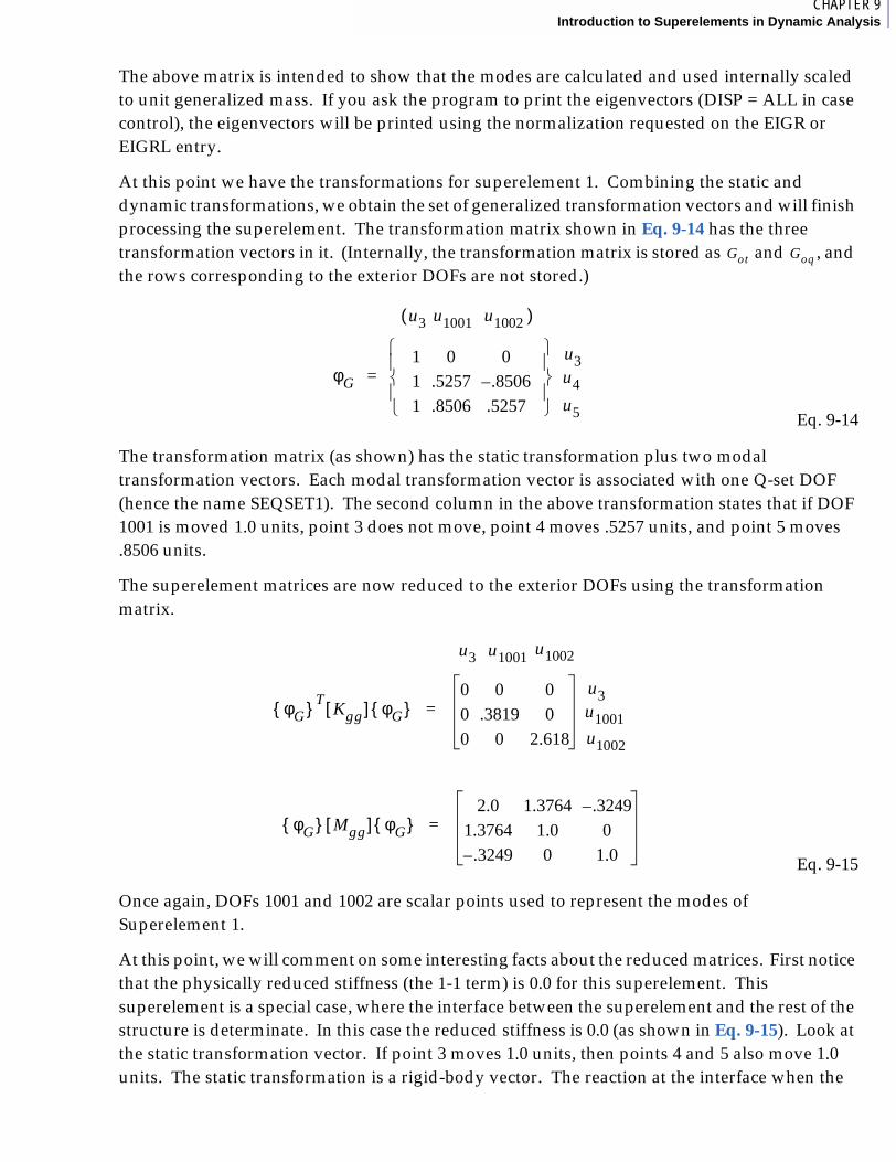
1CHAPTER 9Introduction to Superelements in Dynamic Analysis
The above matrix is intended to show that the modes are calculated and used internally scaled to unit generalized mass. If you ask the program to print the eigenvectors (DISP = ALL in case control), the eigenvectors will be printed using the normalization requested on the EIGR or EIGRL entry.
At this point we have the transformations for superelement 1. Combining the static and dynamic transformations, we obtain the set of generalized transformation vectors and will finish processing the superelement. The transformation matrix shown in Eq. 9-14 has the three transformation vectors in it. (Internally, the transformation matrix is stored as and , and the rows corresponding to the exterior DOFs are not stored.)
Eq. 9-14
The transformation matrix (as shown) has the static transformation plus two modal transformation vectors. Each modal transformation vector is associated with one Q-set DOF (hence the name SEQSET1). The second column in the above transformation states that if DOF 1001 is moved 1.0 units, point 3 does not move, point 4 moves .5257 units, and point 5 moves .8506 units.
The superelement matrices are now reduced to the exterior DOFs using the transformation matrix.
Eq. 9-15
Once again, DOFs 1001 and 1002 are scalar points used to represent the modes of Superelement 1.
At this point, we will comment on some interesting facts about the reduced matrices. First notice that the physically reduced stiffness (the 1-1 term) is 0.0 for this superelement. This superelement is a special case, where the interface between the superelement and the rest of the structure is determinate. In this case the reduced stiffness is 0.0 (as shown in Eq. 9-15). Look at the static transformation vector. If point 3 moves 1.0 units, then points 4 and 5 also move 1.0 units. The static transformation is a rigid-body vector. The reaction at the interface when the
Got Goq
φG
1 0 01 .5257 .8506–
1 .8506 .5257
=u3u4u5
u3( u1001 u1002 )
φG{ } TKgg[ ] φG{ }
0 0 00 .3819 00 0 2.618
=u3
u1002
u3
u1001
u1001 u1002
φG{ } Mgg[ ] φG{ }2.0 1.3764 .3249–
1.3764 1.0 0.3249– 0 1.0
=
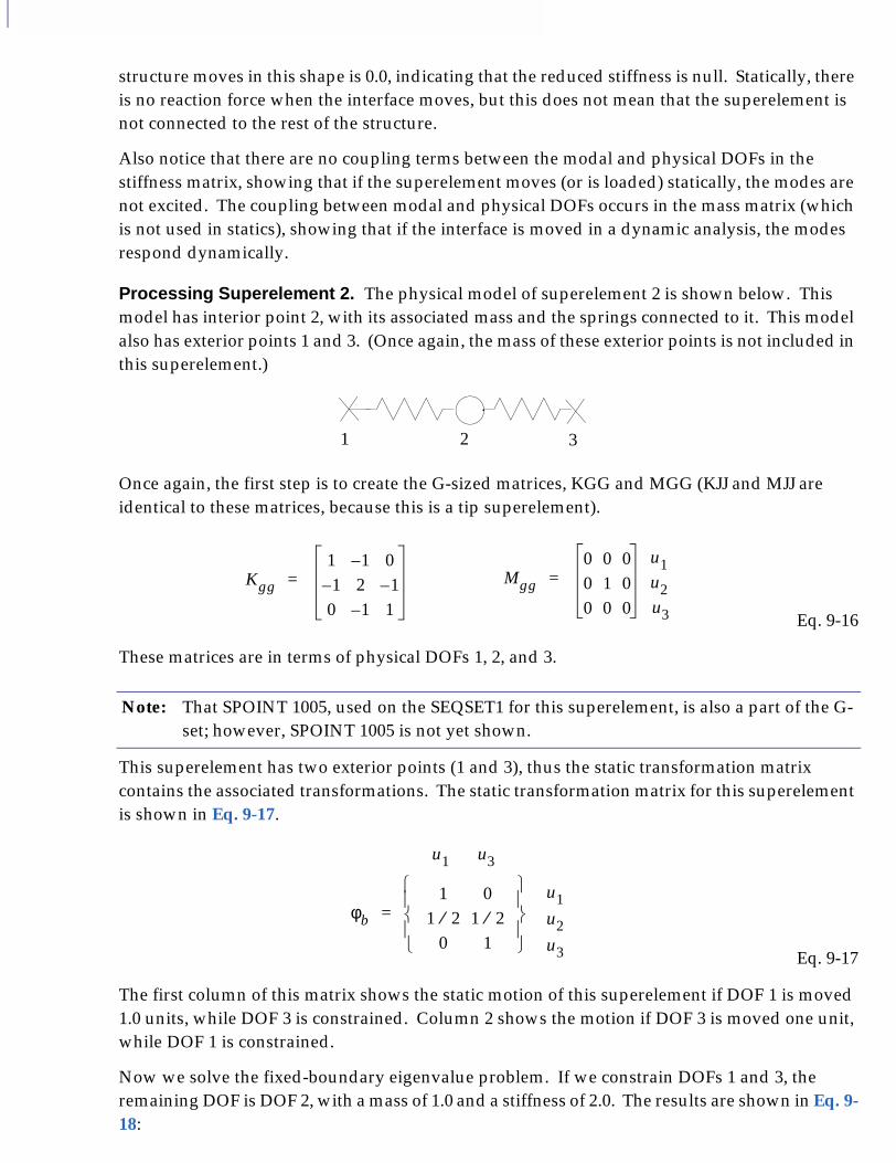
structure moves in this shape is 0.0, indicating that the reduced stiffness is null. Statically, there is no reaction force when the interface moves, but this does not mean that the superelement is not connected to the rest of the structure.
Also notice that there are no coupling terms between the modal and physical DOFs in the stiffness matrix, showing that if the superelement moves (or is loaded) statically, the modes are not excited. The coupling between modal and physical DOFs occurs in the mass matrix (which is not used in statics), showing that if the interface is moved in a dynamic analysis, the modes respond dynamically.
Processing Superelement 2. The physical model of superelement 2 is shown below. This model has interior point 2, with its associated mass and the springs connected to it. This model also has exterior points 1 and 3. (Once again, the mass of these exterior points is not included in this superelement.)
Once again, the first step is to create the G-sized matrices, KGG and MGG (KJJ and MJJ are identical to these matrices, because this is a tip superelement).
Eq. 9-16
These matrices are in terms of physical DOFs 1, 2, and 3.
This superelement has two exterior points (1 and 3), thus the static transformation matrix contains the associated transformations. The static transformation matrix for this superelement is shown in Eq. 9-17.
Eq. 9-17
The first column of this matrix shows the static motion of this superelement if DOF 1 is moved 1.0 units, while DOF 3 is constrained. Column 2 shows the motion if DOF 3 is moved one unit, while DOF 1 is constrained.
Now we solve the fixed-boundary eigenvalue problem. If we constrain DOFs 1 and 3, the remaining DOF is DOF 2, with a mass of 1.0 and a stiffness of 2.0. The results are shown in Eq. 9-18:
Note: That SPOINT 1005, used on the SEQSET1 for this superelement, is also a part of the G-set; however, SPOINT 1005 is not yet shown.
1 2 3
Kgg
1 1– 01– 2 1–
0 1– 1
= Mgg
0 0 00 1 00 0 0
=u1u2u3
φb
1 01 2⁄ 1 2⁄
0 1
=
u1 u3
u1u2u3
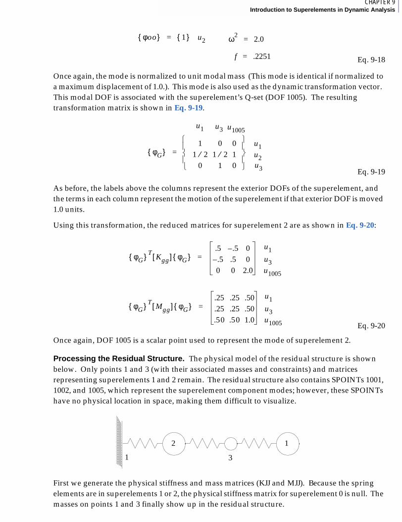
1CHAPTER 9Introduction to Superelements in Dynamic Analysis
Eq. 9-18
Once again, the mode is normalized to unit modal mass (This mode is identical if normalized to a maximum displacement of 1.0.). This mode is also used as the dynamic transformation vector. This modal DOF is associated with the superelement’s Q-set (DOF 1005). The resulting transformation matrix is shown in Eq. 9-19.
Eq. 9-19
As before, the labels above the columns represent the exterior DOFs of the superelement, and the terms in each column represent the motion of the superelement if that exterior DOF is moved 1.0 units.
Using this transformation, the reduced matrices for superelement 2 are as shown in Eq. 9-20:
Eq. 9-20
Once again, DOF 1005 is a scalar point used to represent the mode of superelement 2.
Processing the Residual Structure. The physical model of the residual structure is shown below. Only points 1 and 3 (with their associated masses and constraints) and matrices representing superelements 1 and 2 remain. The residual structure also contains SPOINTs 1001, 1002, and 1005, which represent the superelement component modes; however, these SPOINTs have no physical location in space, making them difficult to visualize.
First we generate the physical stiffness and mass matrices (KJJ and MJJ). Because the spring elements are in superelements 1 or 2, the physical stiffness matrix for superelement 0 is null. The masses on points 1 and 3 finally show up in the residual structure.
φoo{ } 1{ } u2= ω2 2.0=
f .2251=
φG{ }1 0 0
1 2⁄ 1 2⁄ 10 1 0
=
u1 u3 u1005
u1u2u3
φG{ } TKgg[ ] φG{ }
.5 .5– 0.5– .5 00 0 2.0
=
φG{ } TMgg[ ] φG{ }
.25 .25 .50
.25 .25 .50
.50 .50 1.0
=
u1u3u1005
u1u3u1005
1
2
3
1

Eq. 9-21
Note that the residual structure contains the physical DOFs associated with points 1 and 3 and the generalized DOFs representing the upstream superelement modes on SPOINTs 1001, 1002, and 1005.
Now that we have the physical matrices, we need to add the reduced matrices from the upstream superelements. First we add the matrices from superelement 1, which is accomplished by adding the terms from the reduced matrices to the existing terms in the matrices for the associated DOFs. At this point we have intermediate matrices, which are shown in Eq. 9-22:
Eq. 9-22
Now we add the reduced matrices from superelement 2. Once again, we add the terms from the reduced matrices to the existing terms in the locations associated with the exterior DOFs from superelement 2.
We now have the assembly matrices for the residual structure.
KJJ
0 0 0 0 00 0 0 0 00 0 0 0 00 0 0 0 00 0 0 0 0
MJJ
1 0 0 0 00 1 0 0 00 0 0 0 00 0 0 0 00 0 0 0 0
= =
u1u3u1001u1002u1005
Kgg
0 0 0 0 00 0 0 0 00 0 .3819 0 00 0 0 2.618 00 0 0 0 0
=
Mgg
1 0 0 0 00 3 1.3764 .3249– 00 1.3764 1.0 0 00 .3249– 0 1.0 00 0 0 0 0
=
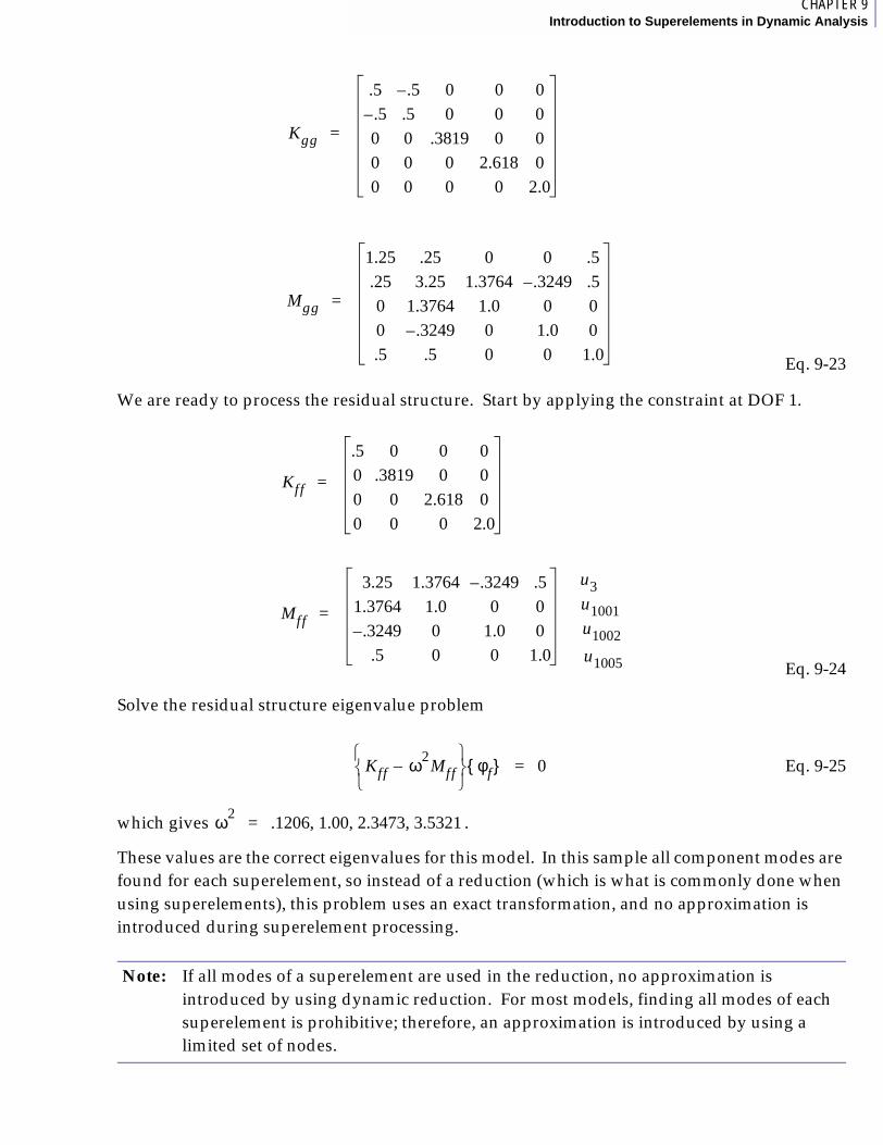
1CHAPTER 9Introduction to Superelements in Dynamic Analysis
Eq. 9-23
We are ready to process the residual structure. Start by applying the constraint at DOF 1.
Eq. 9-24
Solve the residual structure eigenvalue problem
Eq. 9-25
which gives .
These values are the correct eigenvalues for this model. In this sample all component modes are found for each superelement, so instead of a reduction (which is what is commonly done when using superelements), this problem uses an exact transformation, and no approximation is introduced during superelement processing.
Note: If all modes of a superelement are used in the reduction, no approximation is introduced by using dynamic reduction. For most models, finding all modes of each superelement is prohibitive; therefore, an approximation is introduced by using a limited set of nodes.
Kgg
.5 .5– 0 0 0.5– .5 0 0 00 0 .3819 0 00 0 0 2.618 00 0 0 0 2.0
=
Mgg
1.25 .25 0 0 .5.25 3.25 1.3764 .3249– .50 1.3764 1.0 0 00 .3249– 0 1.0 0.5 .5 0 0 1.0
=
Kff
.5 0 0 00 .3819 0 00 0 2.618 00 0 0 2.0
=
Mff
3.25 1.3764 .3249– .51.3764 1.0 0 0
.3249– 0 1.0 0.5 0 0 1.0
=
u3u1001u1002u1005
Kff ω2Mff–
φf{ } 0=
ω2 .1206, 1.00, 2.3473, 3.5321=
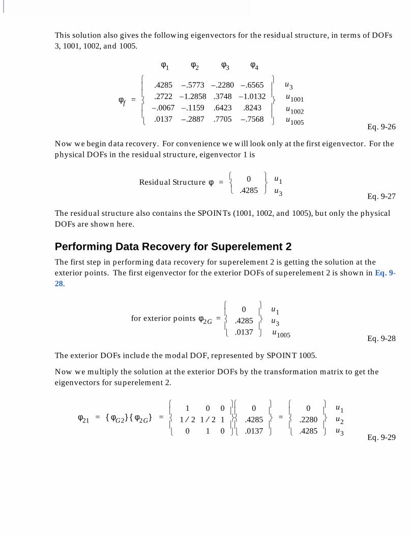
This solution also gives the following eigenvectors for the residual structure, in terms of DOFs 3, 1001, 1002, and 1005.
Eq. 9-26
Now we begin data recovery. For convenience we will look only at the first eigenvector. For the physical DOFs in the residual structure, eigenvector 1 is
Eq. 9-27
The residual structure also contains the SPOINTs (1001, 1002, and 1005), but only the physical DOFs are shown here.
Performing Data Recovery for Superelement 2The first step in performing data recovery for superelement 2 is getting the solution at the exterior points. The first eigenvector for the exterior DOFs of superelement 2 is shown in Eq. 9-28.
Eq. 9-28
The exterior DOFs include the modal DOF, represented by SPOINT 1005.
Now we multiply the solution at the exterior DOFs by the transformation matrix to get the eigenvectors for superelement 2.
Eq. 9-29
φf
.4285 .5773– .2280– .6565–
.2722 1.2858– .3748 1.0132–
.0067– .1159– .6423 .8243.0137 .2887– .7705 .7568–
=
φ1 φ2 φ3 φ4
u3u1001u1002u1005
Residual Structure φ 0.4285
= u1u3
for exterior points φ2G
0.4285.0137
=u1u3u1005
φ21 φG2{ } φ 2G{ }1 0 0
1 2⁄ 1 2⁄ 10 1 0
0
.4285
.0137 0
.2280
.4285
= = =u1u2u3
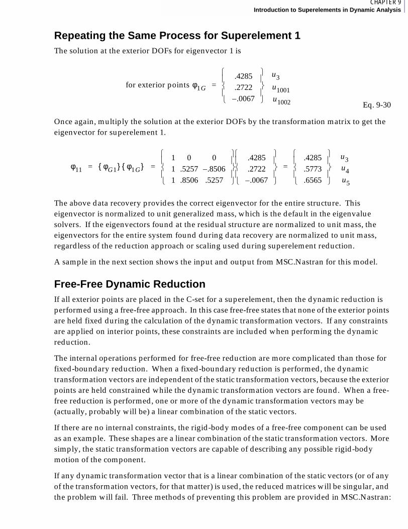
1CHAPTER 9Introduction to Superelements in Dynamic Analysis
Repeating the Same Process for Superelement 1The solution at the exterior DOFs for eigenvector 1 is
Eq. 9-30
Once again, multiply the solution at the exterior DOFs by the transformation matrix to get the eigenvector for superelement 1.
The above data recovery provides the correct eigenvector for the entire structure. This eigenvector is normalized to unit generalized mass, which is the default in the eigenvalue solvers. If the eigenvectors found at the residual structure are normalized to unit mass, the eigenvectors for the entire system found during data recovery are normalized to unit mass, regardless of the reduction approach or scaling used during superelement reduction.
A sample in the next section shows the input and output from MSC.Nastran for this model.
Free-Free Dynamic ReductionIf all exterior points are placed in the C-set for a superelement, then the dynamic reduction is performed using a free-free approach. In this case free-free states that none of the exterior points are held fixed during the calculation of the dynamic transformation vectors. If any constraints are applied on interior points, these constraints are included when performing the dynamic reduction.
The internal operations performed for free-free reduction are more complicated than those for fixed-boundary reduction. When a fixed-boundary reduction is performed, the dynamic transformation vectors are independent of the static transformation vectors, because the exterior points are held constrained while the dynamic transformation vectors are found. When a free-free reduction is performed, one or more of the dynamic transformation vectors may be (actually, probably will be) a linear combination of the static vectors.
If there are no internal constraints, the rigid-body modes of a free-free component can be used as an example. These shapes are a linear combination of the static transformation vectors. More simply, the static transformation vectors are capable of describing any possible rigid-body motion of the component.
If any dynamic transformation vector that is a linear combination of the static vectors (or of any of the transformation vectors, for that matter) is used, the reduced matrices will be singular, and the problem will fail. Three methods of preventing this problem are provided in MSC.Nastran:
for exterior points φ1G
.4285
.2722.0067–
=u3u1001u1002
φ11 φG1{ } φ 1G{ }1 0 01 .5257 .8506–
1 .8506 .5257 .4285
.2722.0067–
.4285
.5773
.6565
= = =u3u4u5
1. Do not calculate the rigid-body modes. Simply, do not request the rigid-body eigenvectors during the calculation of the dynamic transformations. (If employing CMS, use a value greater than 0.0 for the lowest frequency of interest.)
2. Calculate the rigid-body modes, and hope that MSC.Nastran will remove them. Logic is included in the program that attempts to remove any dynamic transformation vectors that are a linear combination of the static transformations. This logic is shown later in this section.
3. Calculate the rigid-body modes, but remove them manually using a SESUP or SUPORT (PARTs) entry (described in the next section). Any exterior DOFs defined on a SESUP entry are not constrained during the calculation of the dynamic transformation vectors. For each DOF listed on an SESUP, MSC.Nastran throws away one dynamic transformation vector, starting with the first one (lowest frequency). We do not recommend this approach, because the program does not check to verify that the thrown away vectors are actually a linear combination of the static transformation vectors. Therefore, elastic modes may be removed unintentionally.
Of the three approaches, not calculating the vectors is the safest.
The internal calculations and an example are shown after the description of mixed boundary dynamic reduction.
Mixed-Boundary Dynamic ReductionThe mixed-boundary dynamic reduction is used whenever exterior DOFs are placed in both the B- and C- and/or R-sets. The eigenvalue problem is now solved, with some (B-set) exterior DOFs constrained and others (C- and R-sets) not constrained. If this approach is used, the problem of dynamic transformation vectors that are a linear combination of the static transformations, (described in the preceding section on free-free dynamic reduction) still exists.
CMS with Exterior DOF in the C- and/or R-SETWhen mixed-boundary or free dynamic reduction is performed, the F-set is partitioned into the V-set and the B-set. The B-set has the same definition as before-exterior DOFs that are constrained during the calculation of the dynamic transformation vectors.
The static transformation is calculated similarly for exterior DOFs, whether they are in the B-, C-, or R-set (subsets of the T-set); therefore, the matrix is independent of the set into which the exterior DOFs are placed.
The calculation of the dynamic transformation depends on the set to which the exterior DOFs belong. If there are any exterior DOFs placed in either the C- or R-set, the program creates a V-set of DOFs for the dynamic reduction step.
The V-set is a combined set for use in dynamic reduction. The V-set consists of all DOFs in the F-set that do not belong in the B-set, therefore, it contains the O-, C-, and R-sets. Any DOF in the V-set is not constrained while calculating the dynamic transformation vectors. The stiffness and mass matrices are partitioned into the V- and B- sets. The V-set stiffness matrix has the form shown in Eq. 9-31.
GOT
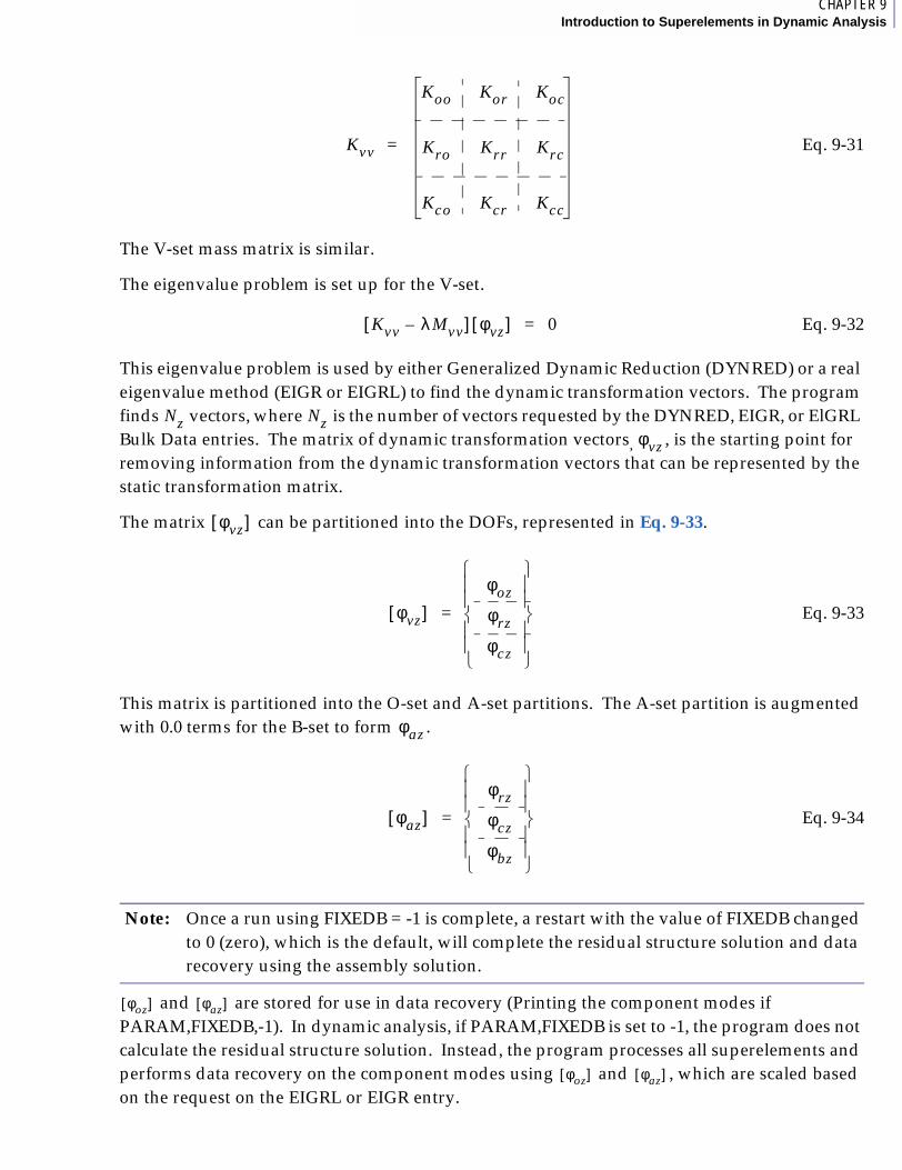
1CHAPTER 9Introduction to Superelements in Dynamic Analysis
Eq. 9-31
The V-set mass matrix is similar.
The eigenvalue problem is set up for the V-set.
Eq. 9-32
This eigenvalue problem is used by either Generalized Dynamic Reduction (DYNRED) or a real eigenvalue method (EIGR or EIGRL) to find the dynamic transformation vectors. The program finds vectors, where is the number of vectors requested by the DYNRED, EIGR, or ElGRL Bulk Data entries. The matrix of dynamic transformation vectors, , is the starting point for removing information from the dynamic transformation vectors that can be represented by the static transformation matrix.
The matrix can be partitioned into the DOFs, represented in Eq. 9-33.
Eq. 9-33
This matrix is partitioned into the O-set and A-set partitions. The A-set partition is augmented with 0.0 terms for the B-set to form .
Eq. 9-34
and are stored for use in data recovery (Printing the component modes if PARAM,FIXEDB,-1). In dynamic analysis, if PARAM,FIXEDB is set to -1, the program does not calculate the residual structure solution. Instead, the program processes all superelements and performs data recovery on the component modes using and , which are scaled based on the request on the EIGRL or EIGR entry.
Note: Once a run using FIXEDB = -1 is complete, a restart with the value of FIXEDB changed to 0 (zero), which is the default, will complete the residual structure solution and data recovery using the assembly solution.
Kvv
Koo Kor Koc
Kro Krr Krc
Kco Kcr Kcc
=
Kvv λ Mvv–[ ] φvz[ ] 0=
Nz Nzφvz
φvz[ ]
φvz[ ]φoz
φrz
φcz
=
φaz
φaz[ ]φrz
φcz
φbz
=
φoz[ ] φaz[ ]
φoz[ ] φaz[ ]
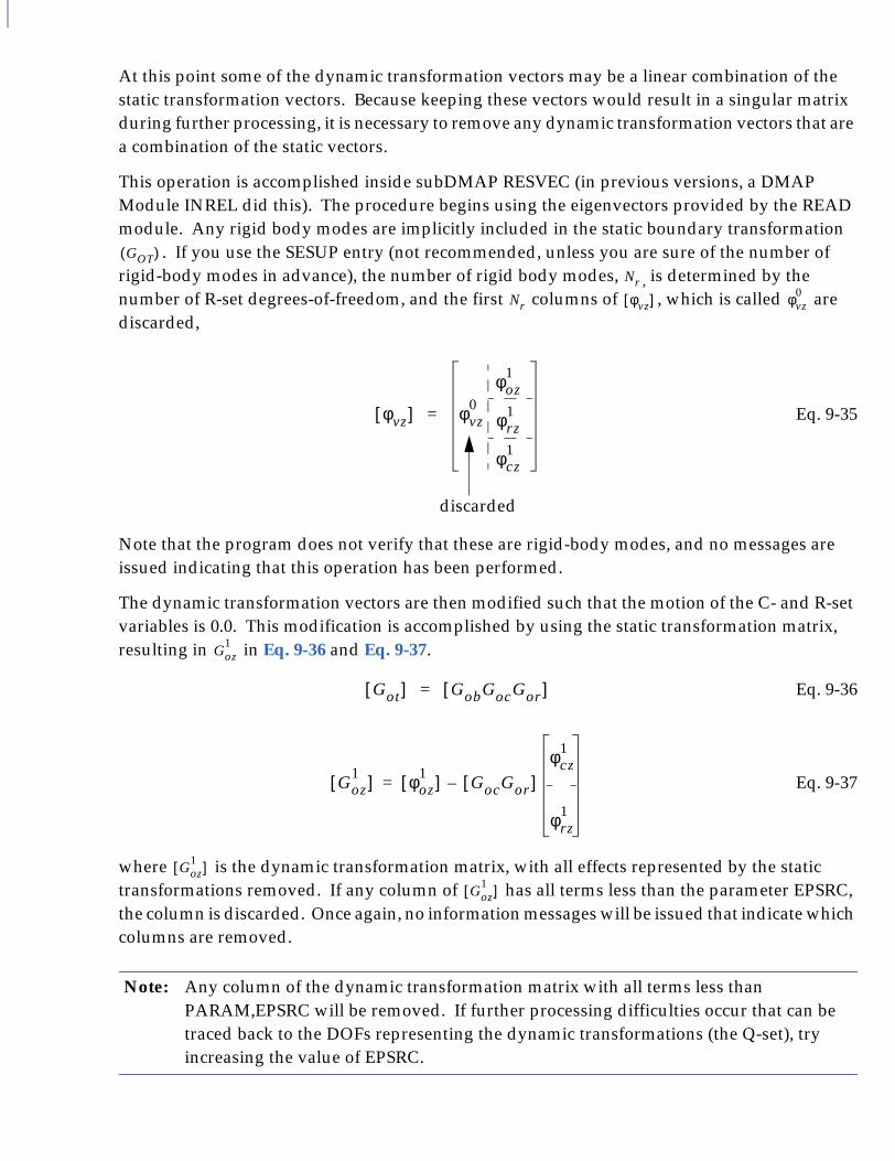
At this point some of the dynamic transformation vectors may be a linear combination of the static transformation vectors. Because keeping these vectors would result in a singular matrix during further processing, it is necessary to remove any dynamic transformation vectors that are a combination of the static vectors.
This operation is accomplished inside subDMAP RESVEC (in previous versions, a DMAP Module INREL did this). The procedure begins using the eigenvectors provided by the READ module. Any rigid body modes are implicitly included in the static boundary transformation
. If you use the SESUP entry (not recommended, unless you are sure of the number of rigid-body modes in advance), the number of rigid body modes, , is determined by the number of R-set degrees-of-freedom, and the first columns of , which is called are discarded,
Eq. 9-35
Note that the program does not verify that these are rigid-body modes, and no messages are issued indicating that this operation has been performed.
The dynamic transformation vectors are then modified such that the motion of the C- and R-set variables is 0.0. This modification is accomplished by using the static transformation matrix, resulting in in Eq. 9-36 and Eq. 9-37.
Eq. 9-36
Eq. 9-37
where is the dynamic transformation matrix, with all effects represented by the static transformations removed. If any column of has all terms less than the parameter EPSRC, the column is discarded. Once again, no information messages will be issued that indicate which columns are removed.
Note: Any column of the dynamic transformation matrix with all terms less than PARAM,EPSRC will be removed. If further processing difficulties occur that can be traced back to the DOFs representing the dynamic transformations (the Q-set), try increasing the value of EPSRC.
GOT( )Nr
Nr φvz[ ] φvz0
φvz[ ] φvz0
φoz1
φrz1
φcz1
=
discarded
Goz1
Got[ ] GobGocGor[ ]=
Goz1[ ] φoz
1[ ]= GocGor[ ]φcz
1
φrz1
–
Goz1[ ]
Goz1[ ]
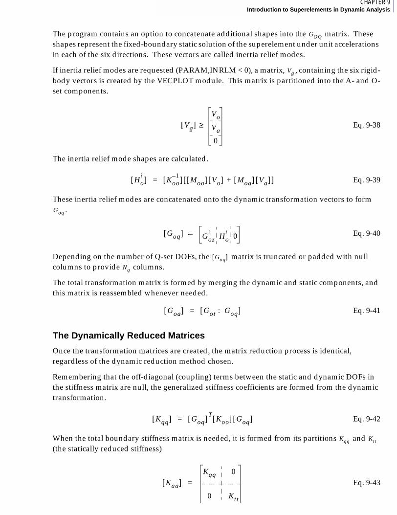
1CHAPTER 9Introduction to Superelements in Dynamic Analysis
The program contains an option to concatenate additional shapes into the matrix. These shapes represent the fixed-boundary static solution of the superelement under unit accelerations in each of the six directions. These vectors are called inertia relief modes.
If inertia relief modes are requested (PARAM,INRLM < 0), a matrix, , containing the six rigid-body vectors is created by the VECPLOT module. This matrix is partitioned into the A- and O-set components.
Eq. 9-38
The inertia relief mode shapes are calculated.
Eq. 9-39
These inertia relief modes are concatenated onto the dynamic transformation vectors to form .
Eq. 9-40
Depending on the number of Q-set DOFs, the matrix is truncated or padded with null columns to provide columns.
The total transformation matrix is formed by merging the dynamic and static components, and this matrix is reassembled whenever needed.
Eq. 9-41
The Dynamically Reduced Matrices
Once the transformation matrices are created, the matrix reduction process is identical, regardless of the dynamic reduction method chosen.
Remembering that the off-diagonal (coupling) terms between the static and dynamic DOFs in the stiffness matrix are null, the generalized stiffness coefficients are formed from the dynamic transformation.
Eq. 9-42
When the total boundary stiffness matrix is needed, it is formed from its partitions and (the statically reduced stiffness)
Eq. 9-43
GOQ
Vg
Vg[ ]Vo
Va
0
≥
Hoi[ ] Koo
1–[ ] Moo[ ] Vo[ ] Moa[ ] Va[ ]+[ ]=
Goq
Goq[ ] Goz1
Hoi 0←
Goq[ ]Nq
Goa[ ] Got : Goq[ ]=
Kqq[ ] Goq[ ] TKoo[ ] Goq[ ]=
Kqq Ktt
Kaa[ ]Kqq 0
0 Ktt
=

There is no coupling between the static and dynamic dof in the stiffness matrix. The static and dynamic degrees-of-freedom are coupled in the mass matrix. The matrix is formed from the equations
Eq. 9-44
If virtual mass effects are to be included, they are added.
The total mass matrix is formed by
Eq. 9-45
The damping matrices and are reduced to the A-set by the MATREDU module, which performs the following operations:
1. Eliminate multipoint constraints
2. Eliminate single-point constraints
3. Partition omitted degrees-of-freedom
Eq. 9-46
4. Perform the reduction using the (combined static and dynamic) transformation matrix
Sample Problem Using Free-Free Component Modal Synthesis
Using a similar model to before (with the addition of density on the elements), we will show how this model is processed using free-free component modal synthesis. In this model ROD elements with density are used in place of the spring elements in the previous example.
Mqq[ ] Goq[ ] TMoo[ ] Goq[ ]=
Mqt[ ] Goq[ ] TMot MooGoa
t+[ ]=
Maa[ ]Mqq Mqt
Mtq Mtt
=
Bgg[ ] Kgg4[ ]
Bgg[ ] Bnn Bnm
Bmn Bmm
=
Bnn[ ] Gmn[ ] TBmmGmn Bmn+[ ]= Bmn[ ] T
Gmn[ ] Bnn[ ]+ +
Bnn[ ]Bff Bfs
Bsf Bss
=
Bff[ ] Baa Bao
Boa Boo
=
Baa[ ] Goa[ ] TBooGoa Boa+[ ]= Boa[ ] T
Goa[ ] Baa[ ]+ +

1CHAPTER 9Introduction to Superelements in Dynamic Analysis
As before, grid points 1 and 3 are assigned to the residual structure. However, now we place them in the C-set for each superelement. Therefore, we are performing free-free CMS. The SECSET1 entry is employed to perform free-free CMS, using the following format:
SECSET1,1,123456,ALL
This entry works only for superelements defined in the Main Bulk Data Section. More information on this entry is provided in the next section.
Process Superelement 1. Grid point 3 is the exterior point.
First we generate the G-sized mass and stiffness. Notice that the mass matrix now contains the mass of the elements; therefore, non-zero mass exists at the exterior points.
As before, we first solve for the static (or constraint) modes.
S. E. #2 S. E. #1
1 2 3 4 5
m1 m2 m3 m4 m5 1.0= = = = =
k1 k2 k3 k4 k5 1.0= = = = =
l1 l2 l3 l4 l5 1.0= = = = =
ρ 2.0=
3 4 5
Mgg
1 0 00 3 00 0 2
Kgg
1 1– 01– 2 1–
0 1– 1
= =
1 1– 01– 2 1–
0 1– 1
1u4
u5 Pb
00
=

Point 3 is exterior, and points 4 and 5 are interior. Partitioning the stiffness into interior and exterior DOFs, we obtain
and solve for the static transformation vector.
As before, if point 3 moves one unit (statically), then points 4 and 5 also move one unit.
Now we need to solve for the elastic modes of the superelement. Because point 3 is in the C-set, we will solve the V-set eigenvalue problem for the free-free modes.
Once again, the V-set is a combination of the C- plus R- plus O-sets; therefore, the free-free eigenequations take the following form.
To solve this problem we need
Koo2 1–
1– 1=
Kob1–
0
=
Koo1– 1 1
1 2=
Φob{ } 1 11 2
1–
0 1
1
=–=;∴
Φb
111
=
ω2Mvv– Kv+[ ] Φ v{ } 0=
ω2– 0 0
0 3ω2– 0
0 0 2ω2–
1 1– 01– 2 1–
0 1– 1
+
Φvv{ } 0=
det1 ω2
– 1– 0
1– 2 3ω2– 1–
0 1– 1 2ω2–
0=
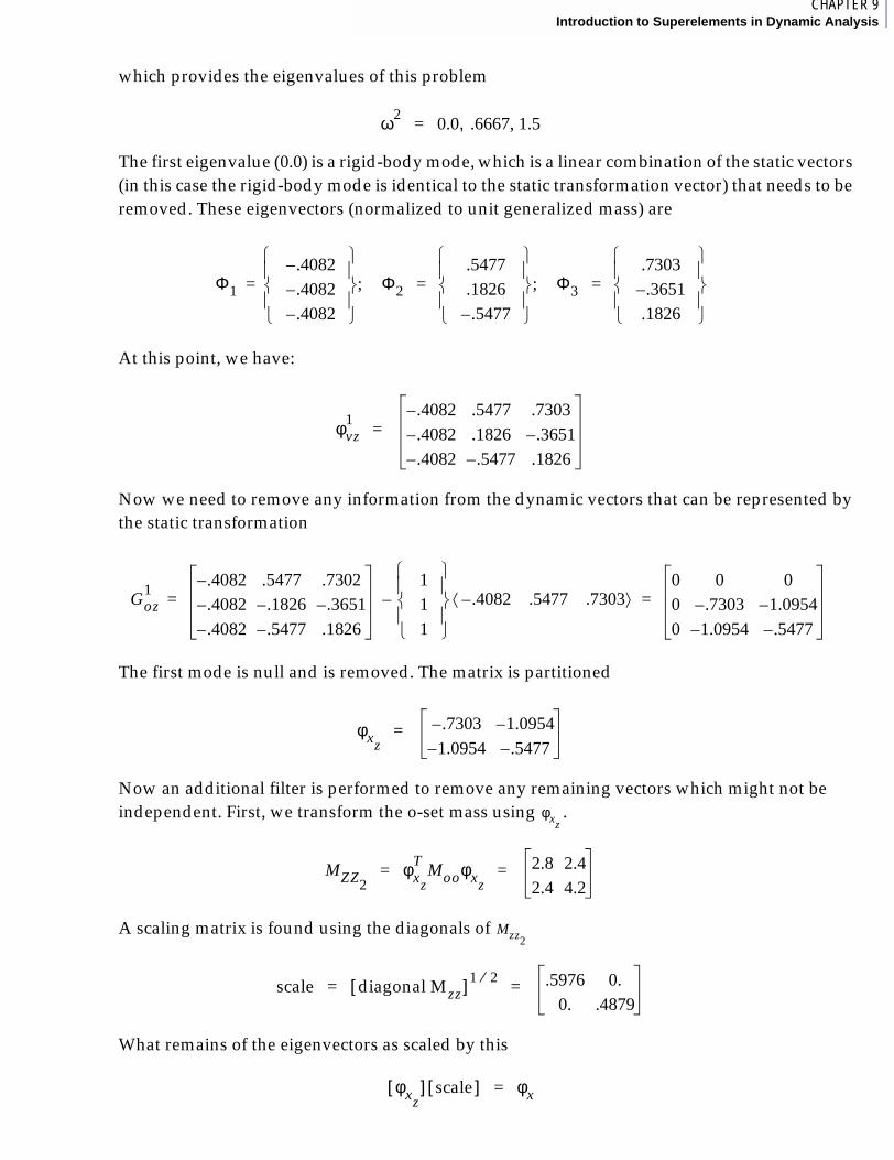
1CHAPTER 9Introduction to Superelements in Dynamic Analysis
which provides the eigenvalues of this problem
The first eigenvalue (0.0) is a rigid-body mode, which is a linear combination of the static vectors (in this case the rigid-body mode is identical to the static transformation vector) that needs to be removed. These eigenvectors (normalized to unit generalized mass) are
At this point, we have:
Now we need to remove any information from the dynamic vectors that can be represented by the static transformation
The first mode is null and is removed. The matrix is partitioned
Now an additional filter is performed to remove any remaining vectors which might not be independent. First, we transform the o-set mass using .
A scaling matrix is found using the diagonals of
What remains of the eigenvectors as scaled by this
ω2 0.0 .6667, 1.5,=
Φ1
.4082–
.4082–
.4082–
Φ; 2=.5477.1826.5477–
Φ3;.7303.3651–
.1826
= =
φvz1 .4082– .5477 .7303
.4082– .1826 .3651–
.4082– .5477– .1826
=
Goz1 .4082– .5477 .7302
.4082– .1826– .3651–
.4082– .5477– .1826
=111
.4082 .5477 .7303–⟨ ⟩0 0 00 .7303– 1.0954–
0 1.0954– .5477–
=–
φxz
.7303– 1.0954–
1.0954– .5477–=
φxz
MZZ2φxz
TMooφxz
2.8 2.42.4 4.2
= =
Mzz2
scale diagonal Mzz[ ] 1 2⁄ .5976 0.0. .4879
= =
φxz[ ] scale[ ] φx=
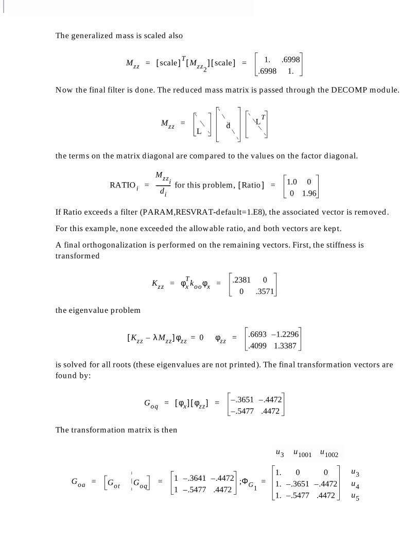
The generalized mass is scaled also
Now the final filter is done. The reduced mass matrix is passed through the DECOMP module.
the terms on the matrix diagonal are compared to the values on the factor diagonal.
for this problem,
If Ratio exceeds a filter (PARAM,RESVRAT-default=1.E8), the associated vector is removed.
For this example, none exceeded the allowable ratio, and both vectors are kept.
A final orthogonalization is performed on the remaining vectors. First, the stiffness is transformed
the eigenvalue problem
is solved for all roots (these eigenvalues are not printed). The final transformation vectors are found by:
The transformation matrix is then
Mzz scale[ ] TMzz2
[ ] scale[ ] 1. .6998.6998 1.
= =
Mzz L
d
LT
=
RATIOi
Mzzi
di-----------= Ratio[ ] 1.0 0
0 1.96=
Kzz φxT
kooφx.2381 0
0 .3571= =
Kzz λMzz–[ ]φzz 0= φzz.6693 1.2296–
.4099 1.3387=
Goq φx[ ] φzz[ ] .3651– .4472–
.5477– .4472= =
Goa Got Goq1 .3641– .4472–
1 .5477– .4472ΦG1
1. 0 01. .3651– .4472–
1. .5477– .4472
=;= =u3u4u5
u3 u1001 u1002
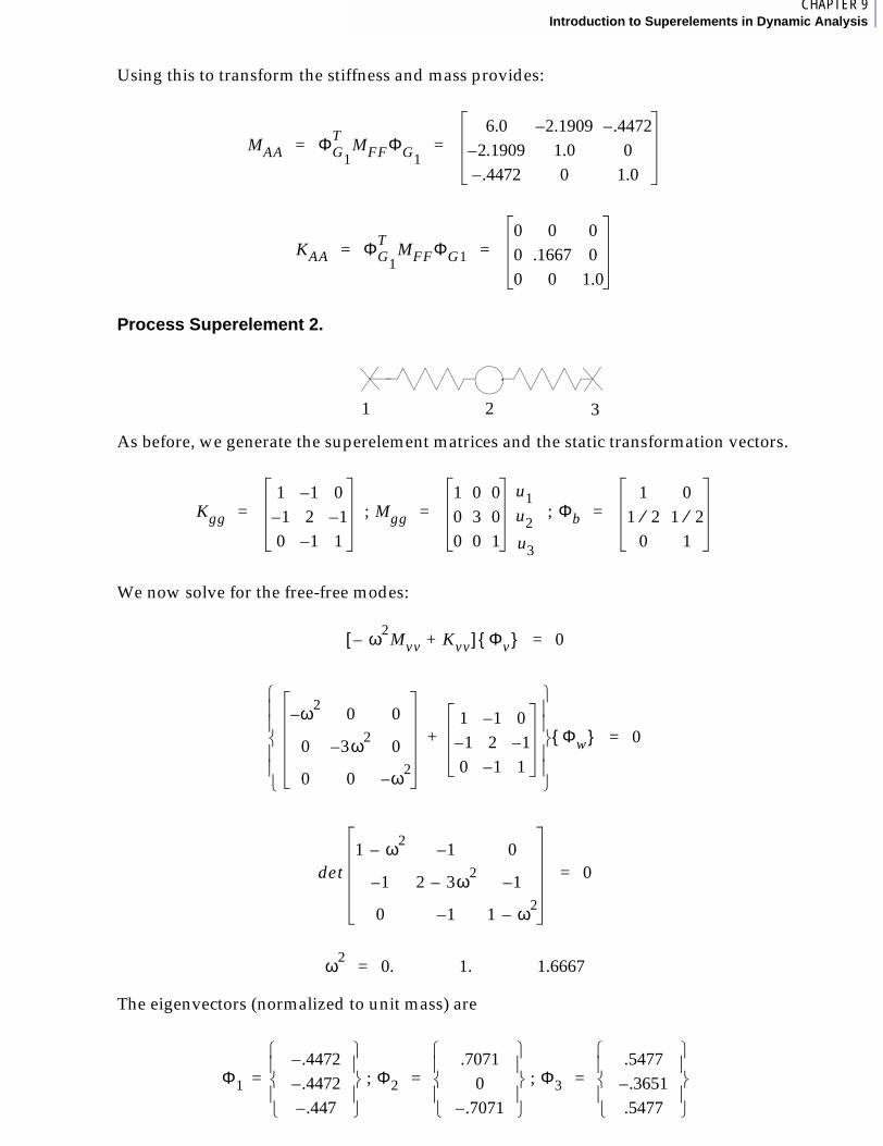
1CHAPTER 9Introduction to Superelements in Dynamic Analysis
Using this to transform the stiffness and mass provides:
Process Superelement 2.
As before, we generate the superelement matrices and the static transformation vectors.
We now solve for the free-free modes:
The eigenvectors (normalized to unit mass) are
MAA ΦG1
TMFFΦG1
6.0 2.1909– .4472–
2.1909– 1.0 0.4472– 0 1.0
= =
KAA ΦG1
TMFFΦG1
0 0 00 .1667 00 0 1.0
= =
1 2 3
Kgg
1 1– 01– 2 1–
0 1– 1
Mgg;1 0 00 3 00 0 1
Φb;1 0
1 2⁄ 1 2⁄0 1
= = =u1u2u3
ω2Mvv– Kvv+[ ] Φ v{ } 0=
ω2– 0 0
0 3ω2– 0
0 0 ω2–
1 1– 01– 2 1–
0 1– 1
+
Φw{ } 0=
det1 ω2
– 1– 0
1– 2 3ω2– 1–
0 1– 1 ω2–
0=
ω2 0.= 1. 1.6667
Φ1
.4472–
.4472–
.447–
; Φ2=.7071
0.7071–
; Φ3
.5477.3651–
.5477
= =
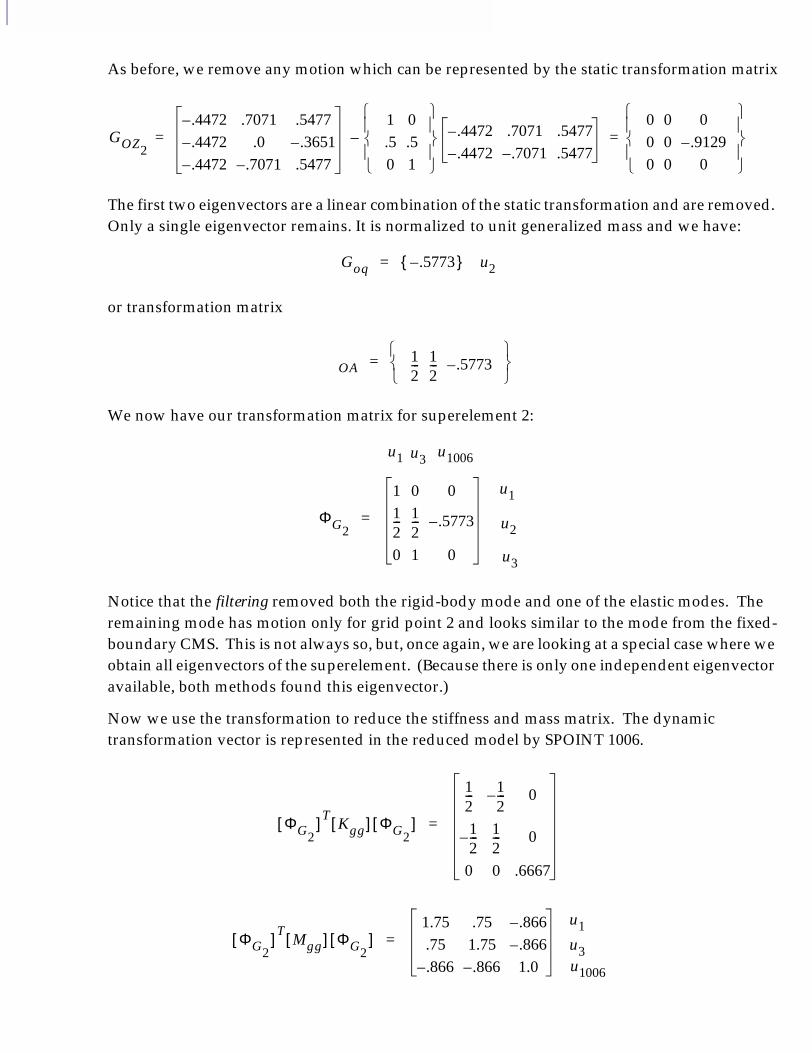
As before, we remove any motion which can be represented by the static transformation matrix
The first two eigenvectors are a linear combination of the static transformation and are removed. Only a single eigenvector remains. It is normalized to unit generalized mass and we have:
or transformation matrix
We now have our transformation matrix for superelement 2:
Notice that the filtering removed both the rigid-body mode and one of the elastic modes. The remaining mode has motion only for grid point 2 and looks similar to the mode from the fixed-boundary CMS. This is not always so, but, once again, we are looking at a special case where we obtain all eigenvectors of the superelement. (Because there is only one independent eigenvector available, both methods found this eigenvector.)
Now we use the transformation to reduce the stiffness and mass matrix. The dynamic transformation vector is represented in the reduced model by SPOINT 1006.
GOZ2
.4472– .7071 .5477
.4472– .0 .3651–
.4472– .7071– .5477
=1 0.5 .50 1
.4472– .7071 .5477
.4472– .7071– .5477
0 0 00 0 .9129–
0 0 0
=–
Goq .5773–{ }= u2
OA12--- 1
2--- .5773–
=
ΦG2
1 0 012--- 1
2--- .5773–
0 1 0
=
u1
u2
u3
u1 u3 u1006
ΦG2[ ] T
Kgg[ ] Φ G2[ ]
12--- 1
2---– 0
12---– 1
2--- 0
0 0 .6667
=
ΦG2[ ] T
Mgg[ ] Φ G2[ ]
1.75 .75 .866–
.75 1.75 .866–
.866– .866– 1.0
=u1u3u1006

1CHAPTER 9Introduction to Superelements in Dynamic Analysis
Residual Structure
Once again, the model of the residual structure is:
All the remaining grid points are in this model (points 1 and 3). All elements have been placed in upstream superelements, and we have the two sets of reduced matrices, representing superelements 1 and 2. We also have scalar points 1001, 1002, and 1006, representing the modes from the superelements.
First we form the physical mass and stiffness for the residual structure.
Add the reduced matrices from superelement 1:
1
2
3
1
Kjj
0 0 0 0 00 0 0 0 00 0 0 0 00 0 0 0 00 0 0 0 0
=
Mjj
1 0 0 0 00 1 0 0 00 0 0 0 00 0 0 0 00 0 0 0 0
=
u1u3u1001u1002u1006
Kgg
0 0 0 0 00 0 0 0 00 0 .1667 0 00 0 0 1.0 00 0 0 0 0
=
u1u3u1001u1002u1006
Mgg
1 0 0 0 00 7.0 2.1909– .4472– 00 2.1909– 1.0 0 00 .4472– 0 1.0 00 0 0 0 0
=
u1u3u1001u1002u1006
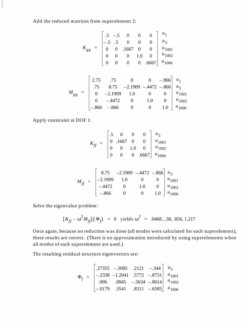
Add the reduced matrices from superelement 2:
Apply constraint at DOF 1:
Solve the eigenvalue problem:
yields , .38, .856, 1.217
Once again, because no reduction was done (all modes were calculated for each superelement), these results are correct. (There is no approximation introduced by using superelements when all modes of each superelement are used.)
The resulting residual structure eigenvectors are:
Kgg
.5 .5– 0 0 0.5– .5 0 0 00 0 .1667 0 00 0 0 1.0 00 0 0 0 .6667
=
u1u3u1001u1002u1006
Mgg
2.75 .75 0 0 .866–
.75 8.75 2.1909– .4472– .866–
0 2.1909– 1.0 0 00 .4472– 0 1.0 0
.866– .866– 0 0 1.0
=
u1u3u1001u1002u1006
Kff
.5 0 0 00 .1667 0 00 0 1.0 00 0 0 .6667
=
u3u1001u1002u1006
Mff
8.75 2.1909– .4472– .866–
2.1909– 1.0 0 0.4472– 0 1.0 0.866– 0 0 1.0
=
u3u1001u1002u1006
Kff ω2Mff–[ ] Φ f{ } 0= ω2 .0468=
Φf
.27355 .3085– .2121 .344–
.2338– 1.2041– .5772 .8731–
.006 .0845 .5634– .8614–
.0179– .3541 .8311 .6585–
=
u3u1001u1002u1006
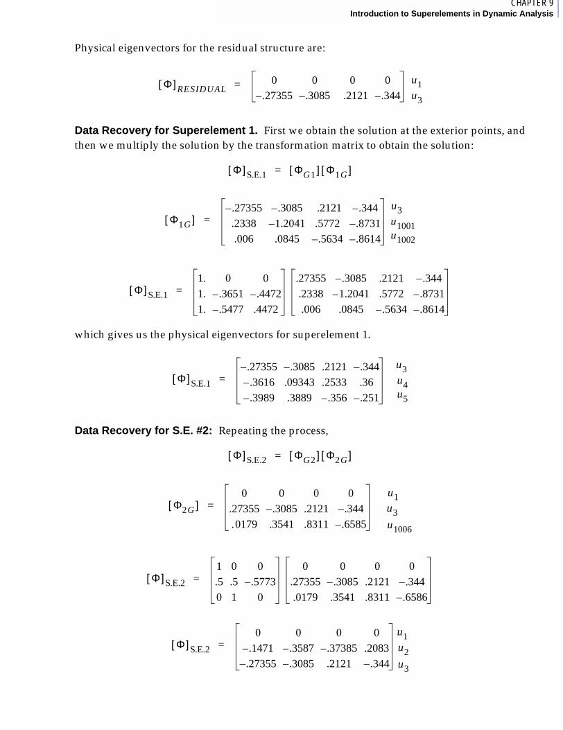
1CHAPTER 9Introduction to Superelements in Dynamic Analysis
Physical eigenvectors for the residual structure are:
Data Recovery for Superelement 1. First we obtain the solution at the exterior points, and then we multiply the solution by the transformation matrix to obtain the solution:
which gives us the physical eigenvectors for superelement 1.
Data Recovery for S.E. #2: Repeating the process,
Φ[ ] RESIDUAL0 0 0 0
.27355– .3085– .2121 .344–= u1
u3
Φ[ ] S.E.1 ΦG1[ ] Φ 1G[ ]=
Φ1G[ ].27355– .3085– .2121 .344–
.2338 1.2041– .5772 .8731–
.006 .0845 .5634– .8614–
= u3 u1001 u1002
Φ[ ] S.E.1
1. 0 01. .3651– .4472–
1. .5477– .4472
.27355 .3085– .2121 .344–
.2338 1.2041– .5772 .8731–
.006 .0845 .5634– .8614–
=
Φ[ ] S.E.1
.27355– .3085– .2121 .344–
.3616– .09343 .2533 .36
.3989– .3889 .356– .251–
=u3u4u5
Φ[ ] S.E.2 ΦG2[ ] Φ 2G[ ]=
Φ2G[ ]0 0 0 0
.27355 .3085– .2121 .344–
.0179 .3541 .8311 .6585–
=u1u3u1006
Φ[ ] S.E.2
1 0 0.5 .5 .5773–
0 1 0
0 0 0 0.27355 .3085– .2121 .344–
.0179 .3541 .8311 .6586–
=
Φ[ ] S.E.2
0 0 0 0.1471– .3587– .37385– .2083
.27355– .3085– .2121 .344–
=u1u2u3

we obtain
which compares to the results from an MSC.Nastran run for this model.
The basic idea of how superelements are processed in a dynamic solution has been presented. Once again, you have the option to either perform a static reduction (the default) or a dynamic reduction. If you choose a dynamic reduction, you can treat the exterior DOFs any way you wish (constrained or not constrained) during the calculation of the dynamic transformation.
If you perform a dynamic transformation, the accuracy of the results depends on your skill and engineering insight. As you have seen, obtaining all modes for each superelement gives the exact answer. If you obtain fewer modes, you are introducing approximations into the problem. Both how you treat the exterior DOFs and the number of eigenvectors obtained have an effect on the solution quality. If you do not treat the exterior DOFs carefully, you can compensate with a large number of component modes. Likewise, if you do not calculate many component modes, proper treatment of the exterior DOFs can improve the accuracy.
Unfortunately, there is no set method that works best for all problems. The default method of dynamic reduction (Craig-Bampton CMS) works well for most problems; however, there will always be problems for which dynamic reduction does not work well.
The number of methods for calculating dynamic transformation vectors is unlimited. Many of these methods are used in industry. The best summary of the standard methods of calculation are in Craig’s text, see “References” in Appendix A.
Φ[ ] FULL BY HAND
0 0 0 0.1471– .3587– .37385– .2083
.27355– .3085– .2121 .344–
.3616– .09343 .2533 .36
.3989– .3889 .356– .251–
=
u1u2u3u4u5
Φ[ ] MSC/NASTRAN
0 0 0 0.1471 .3587– .3737 .2082.2735 .3085– .212– .344–
.3616 .0933 .2533– .3601
.3989 .388 .3559 .251–
=
u1u2u3u4u5
MSC.Nastran Superelements User’s Guide
CHAPTER
10 Input and Output for Dynamic Reduction
■ Case Control for Dynamic Reduction
■ Single-Level Dynamic Reduction
■ Multilevel Dynamic Reduction
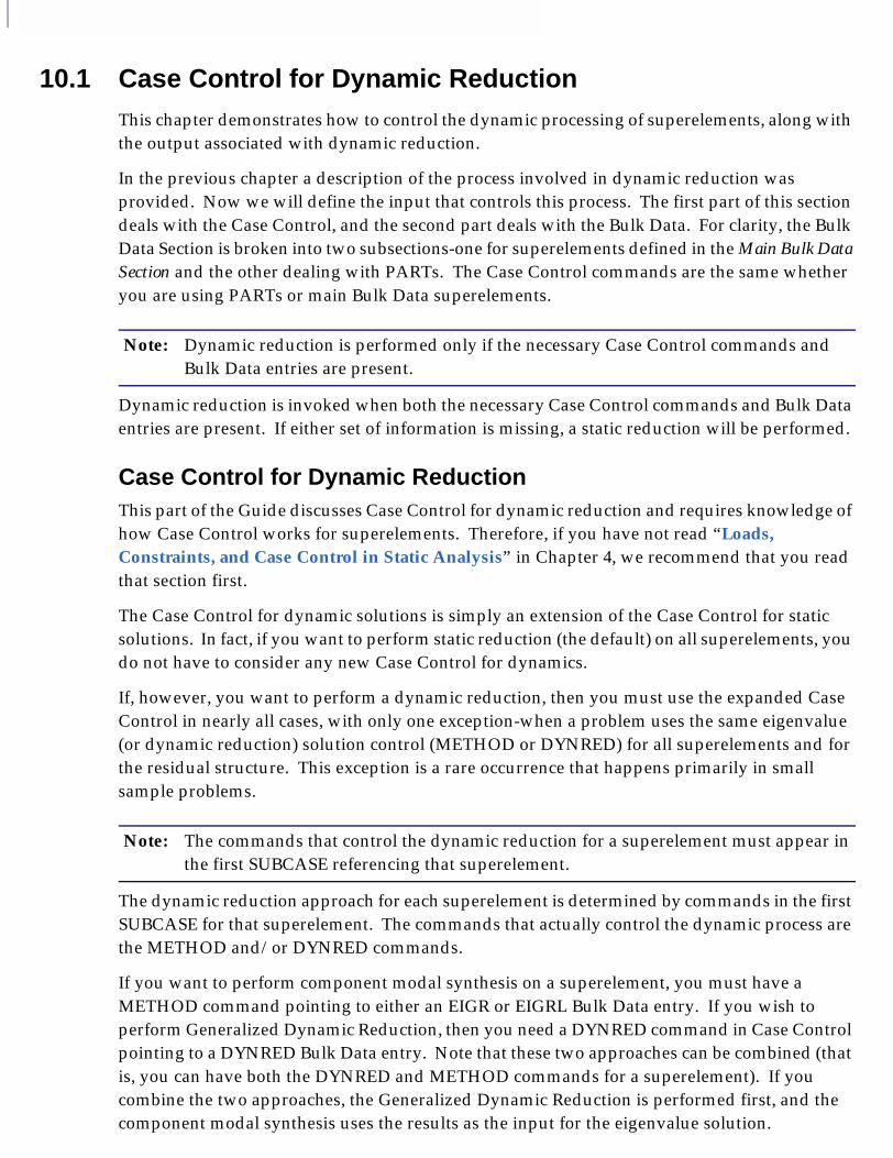
10.1 Case Control for Dynamic ReductionThis chapter demonstrates how to control the dynamic processing of superelements, along with the output associated with dynamic reduction.
In the previous chapter a description of the process involved in dynamic reduction was provided. Now we will define the input that controls this process. The first part of this section deals with the Case Control, and the second part deals with the Bulk Data. For clarity, the Bulk Data Section is broken into two subsections-one for superelements defined in the Main Bulk Data Section and the other dealing with PARTs. The Case Control commands are the same whether you are using PARTs or main Bulk Data superelements.
Dynamic reduction is invoked when both the necessary Case Control commands and Bulk Data entries are present. If either set of information is missing, a static reduction will be performed.
Case Control for Dynamic ReductionThis part of the Guide discusses Case Control for dynamic reduction and requires knowledge of how Case Control works for superelements. Therefore, if you have not read “Loads, Constraints, and Case Control in Static Analysis” in Chapter 4, we recommend that you read that section first.
The Case Control for dynamic solutions is simply an extension of the Case Control for static solutions. In fact, if you want to perform static reduction (the default) on all superelements, you do not have to consider any new Case Control for dynamics.
If, however, you want to perform a dynamic reduction, then you must use the expanded Case Control in nearly all cases, with only one exception-when a problem uses the same eigenvalue (or dynamic reduction) solution control (METHOD or DYNRED) for all superelements and for the residual structure. This exception is a rare occurrence that happens primarily in small sample problems.
The dynamic reduction approach for each superelement is determined by commands in the first SUBCASE for that superelement. The commands that actually control the dynamic process are the METHOD and/or DYNRED commands.
If you want to perform component modal synthesis on a superelement, you must have a METHOD command pointing to either an EIGR or EIGRL Bulk Data entry. If you wish to perform Generalized Dynamic Reduction, then you need a DYNRED command in Case Control pointing to a DYNRED Bulk Data entry. Note that these two approaches can be combined (that is, you can have both the DYNRED and METHOD commands for a superelement). If you combine the two approaches, the Generalized Dynamic Reduction is performed first, and the component modal synthesis uses the results as the input for the eigenvalue solution.
Note: Dynamic reduction is performed only if the necessary Case Control commands and Bulk Data entries are present.
Note: The commands that control the dynamic reduction for a superelement must appear in the first SUBCASE referencing that superelement.
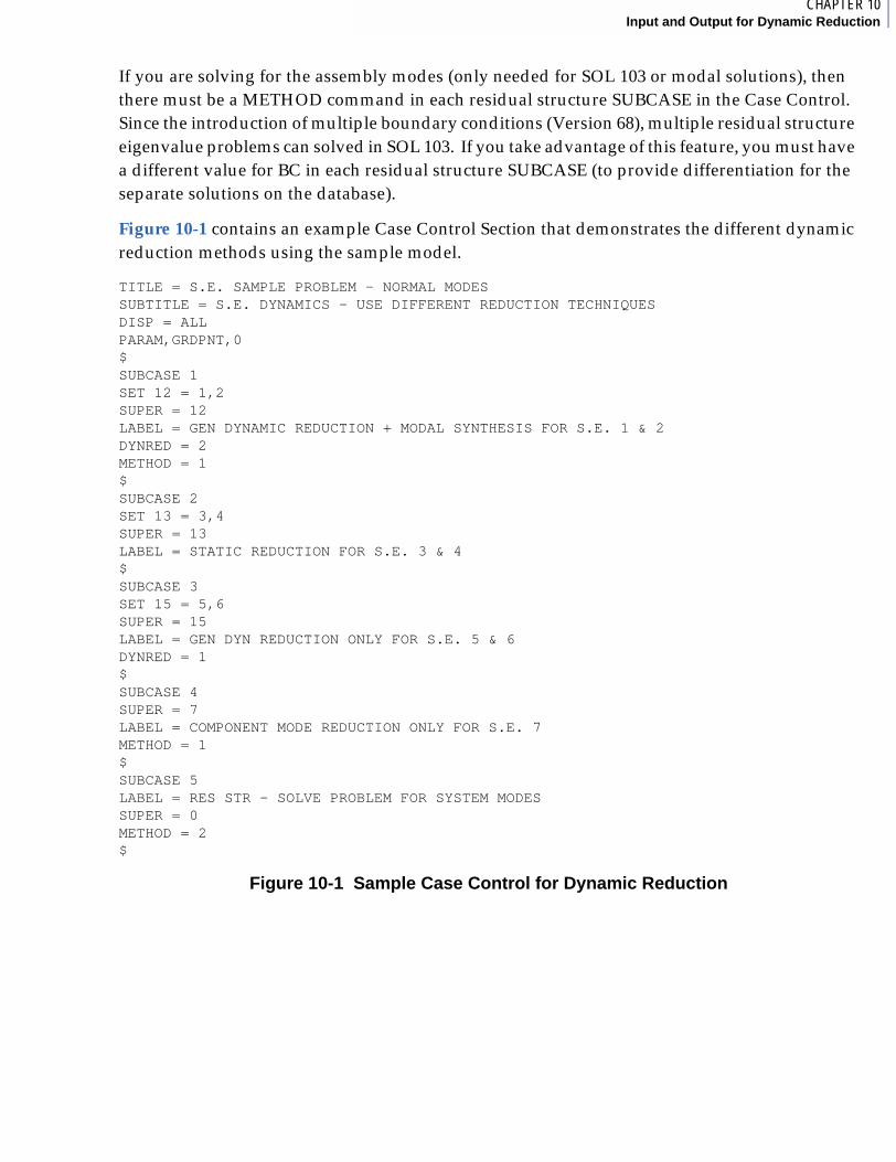
1CHAPTER 10Input and Output for Dynamic Reduction
If you are solving for the assembly modes (only needed for SOL 103 or modal solutions), then there must be a METHOD command in each residual structure SUBCASE in the Case Control. Since the introduction of multiple boundary conditions (Version 68), multiple residual structure eigenvalue problems can solved in SOL 103. If you take advantage of this feature, you must have a different value for BC in each residual structure SUBCASE (to provide differentiation for the separate solutions on the database).
Figure 10-1 contains an example Case Control Section that demonstrates the different dynamic reduction methods using the sample model.
TITLE = S.E. SAMPLE PROBLEM - NORMAL MODESSUBTITLE = S.E. DYNAMICS - USE DIFFERENT REDUCTION TECHNIQUESDISP = ALLPARAM,GRDPNT,0$SUBCASE 1SET 12 = 1,2SUPER = 12LABEL = GEN DYNAMIC REDUCTION + MODAL SYNTHESIS FOR S.E. 1 & 2DYNRED = 2METHOD = 1$SUBCASE 2SET 13 = 3,4SUPER = 13LABEL = STATIC REDUCTION FOR S.E. 3 & 4$SUBCASE 3SET 15 = 5,6SUPER = 15LABEL = GEN DYN REDUCTION ONLY FOR S.E. 5 & 6DYNRED = 1$SUBCASE 4SUPER = 7LABEL = COMPONENT MODE REDUCTION ONLY FOR S.E. 7METHOD = 1$SUBCASE 5LABEL = RES STR - SOLVE PROBLEM FOR SYSTEM MODESSUPER = 0METHOD = 2$
Figure 10-1 Sample Case Control for Dynamic Reduction

If the input file has the correct Bulk Data entries, the above Case Control Section requests the following:
Of the above approaches, component modal synthesis is most commonly used; therefore, your SUBCASEs will usually resemble SUBCASE 4 (above).
SUBCASE 1 (Applies to superelements 1 and 2.) This SUBCASE requests Generalized Dynamic Reduction using DYNRED set 2 to be performed, followed by component modal synthesis using eigenvalue METHOD 1. (Note: Generalized Dynamic Reduction is no longer recommended, this sample simply shows the commands.)
SUBCASE 2 (Applies to superelements 3 and 4.) Because there are no commands requesting a dynamic reduction, these superelements have a static reduction only.
SUBCASE 3 (Applies to superelements 5 and 6.) This SUBCASE instructs the program to perform Generalized Dynamic Reduction for these superelements. (Note: Generalized Dynamic Reduction is no longer recommended, this sample simply shows the commands.)
SUBCASE 4 (Applies to superelement 7). This SUBCASE is the most commonly used form, which performs component modal synthesis. In this case the program has been instructed to use the eigenvalue solution described on EIGRL (or EIGR) 1 to calculate the modes of superelement 7.
SUBCASE 5 (Applies to the residual structure.) This SUBCASE instructs the program to use eigenvalue METHOD 2 to solve for the assembly modes at the residual structure.
1CHAPTER 10Input and Output for Dynamic Reduction
10.2 Single-Level Dynamic ReductionThe Bulk Data entries for single- and multilevel dynamic reduction are similar. These entries are shown in different sections to emphasize the differences in the approaches. As mentioned before, the Case Control is independent of the type of tree used (single- or multilevel).
In a single-level dynamic solution, all the superelements attach directly to the residual structure. Therefore, the component modes are passed to the residual structure for the system solution. In multilevel dynamics it is possible to create assemblies, where component modes from upstream superelements are coupled into a superelement to obtain the assembly modes, before the reduced matrices are passed to the residual structure.
In a single-level tree the DOFs that represent the modes of the components must be interior to the residual and exterior to the superelements, which is accomplished using the following methods.
Bulk Data Entries for Single-Level Dynamic Reduction of Main Bulk Data SuperelementsTo perform a dynamic reduction on a superelement-in addition to the required Case Control commands-you need to define the DOFs that will represent the dynamic transformation vectors (component modes). You also need to define how you want to treat the exterior DOFs during the eigenvalue solution (the default is fixed-boundary).
The following Bulk Data entries are used when performing dynamic reduction of superelements defined in the Main Bulk Data Section.
SEQSET and/or SEQSET1 one or both of these entries can be used to define the DOFs that will represent the superelement dynamic transformation vectors (component modes) in subsequent processing. These entries point to SPOINTs and/or grid points that are interior to the residual. If the model is defined using only main Bulk Data superelements, grid points can be used. If any PARTs exist, then only SPOINTs can be used.
Note: For each DOF listed on SESUP entries, one dynamic transformation vector (starting with the lowest natural frequency) is removed. Because the program performs no checking, we do not recommend this approach.
SEBSET and/or SEBSET1 list of exterior DOFs that are placed in the superelement’s B-set, these dof are constrained during the calculation of the dynamic transformation. (Default = all exterior DOFs)
SECSET and/or SECSET1 list of exterior DOFs that are placed in the superelement’s C-set, these are not constrained during the calculation of the dynamic transformation vectors. (Default = none)

For main Bulk Data superelements, component modes must be attached to either grid points or SPOINTs (with the exception that if PARTs exist, then grid points cannot be used; the SENQSET entry can be used for both main Bulk Data superelements and PARTs).
To attach the component modes to grid or SPOINTs, use the SEQSET and/or SEQSET1 entries. When using these entries, you will identify the superelement with which you are working and the selected DOFs for the grids or SPOINTs (0) that will represent the component modes. Make sure you select a sufficient number of DOFs to represent all of the component modes you are calculating, or the unrepresented modes will not be included in the solution. In a single-level process, the GRID and SPOINTs that represent the component modes must be interior to the residual structure.
If you use GRID points to represent the component modes for a superelement, these grids should have no attached structural elements. If they have structural elements attached, then you will encounter User Fatal Message 5290, indicating that you are attaching a structural element to a Q-set DOF.
*** USER FATAL MESSAGE 5290 (GPSP) EXTERNAL ID = 1001 DOF = 1 IS IN THE Q-SET, BUT HAS A STIFFNESS TERM BEFORE REDUCTION. ^^^ USER FATAL MESSAGE 9032 (ERRPH1) - RUN IS TERMINATED DUE TO MESSAGE(S) ABOVE. TO CONTINUE PROCESSING ALL SUPERELEMENTS, INSERT PARAM,ERROR,0 INTO BULK DATA.
The above message indicates that grid point 1001, which is in the Q-set for the current superelement, has a stiffness term before the component modes are calculated and the run is terminated. Notice that the message mentions PARAM,ERROR can be used to continue the run. A value of 0 for PARAM,ERROR instructs the program to terminate processing of the current superelement when a FATAL message in encountered. However, the run will continue to process other superelements until it can go no further. If you use this parameter, you should always look at the output file carefully to verify that you did not encounter a FATAL error.
SESUP list of exterior DOFs that are placed into the superelement R-set. These DOFs are not constrained during the calculation of the dynamic transformation vectors. However, for each DOF listed on the SESUP entry, one dynamic transformation vector (starting with the first one) is removed without any checking performed.
SENQSET list of the number of automatically generated Q-set DOFs for selected superelements or all superelements. This entry can be used only if there are one or more PARTs in the model. If used, this entry will automatically generate internal DOFs for the Q-set for selected superelements. These DOFs are passed to the residual structure, with no coupling to downstream superelements until the residual structure is processed. Therefore, this entry may not be the best choice for multilevel dynamic analysis.
GRID and/or SPOINT You must define the degrees-of-freedom MSC.Nastran will use for the component modes (Note: If you use the SENQSET, this step is not required.)
1CHAPTER 10Input and Output for Dynamic Reduction
If your model is defined using main Bulk Data superelements only, then you can easily use SPOINTs for the component modes. When a model is defined using main Bulk Data superelements only, all SPOINTs are interior to the residual structure by definition and cannot be interior to any other superelement, which is different from how a model with PARTs will behave. In a model with PARTs, SPOINTs can be interior to any superelement.
The following lines show how SPOINTs can be used to define the Q-set DOFs for a superelement.
SPOINT,1001,thru,1010SEQSET1,1,0,1001,thru,1010
The above code creates 10 SPOINTs (1001 through 1010) and instructs the program to use these SPOINTs to represent the first 10 modes from superelement 10.
Samples of Single-Level Dynamic Reduction for Main Bulk Data SuperelementsFirst we will use a model of a cantilever beam to show the input for the different approaches. This model is also used to generate the table comparing results of different reduction methods in “Introduction to Superelements in Dynamic Analysis” on page 141. In “Introduction to Superelements in Dynamic Analysis” on page 141 several runs were made for each dynamic reduction approach, using a different number of modes calculated at the superelement level. All of these runs are performed using SOL 103 (SEMODES).
The approaches we will use are:
• static reduction only (seg10_a.dat)
• Fixed-boundary CMS (seg10_b1.dat)
• Free-free CMS (seg10_c1.dat)
• mixed-boundary CMS (seg10_d1.dat)
The following listing is the model used for this example; this model is a cantilever beam, as shown in Figure 9-1. The model is divided into two superelements (1 and 2) using SESET entries. Superelement 1 has interior points 7 through 11, and superelement 2 has interior points 1 through 5. Both superelements have grid point 6 as their exterior point.
File cantbeam.dat - Input Model for the Examplesseset,1,7,thru,11seset,2,1,thru,5$PARAM,GRDPNT,0SPC 1 1 123456 0.PBAR 1 1 0.1 0.01 0.01 0.001 0. MAT1 1 2.9E+7 1.1E+7 0.327.357E-4 6.E-6 70. MAT4 15.787E-5 0.1167.357E-4GRDSET 1345
Note: If a model is defined using main Bulk Data superelements only, then SPOINTS are (by definition) interior to the residual structure.
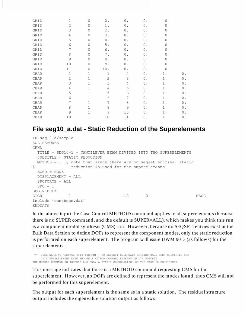
GRID 1 0 0. 0. 0. 0 GRID 2 0 1. 0. 0. 0 GRID 3 0 2. 0. 0. 0 GRID 4 0 3. 0. 0. 0 GRID 5 0 4. 0. 0. 0 GRID 6 0 5. 0. 0. 0 GRID 7 0 6. 0. 0. 0 GRID 8 0 7. 0. 0. 0 GRID 9 0 8. 0. 0. 0 GRID 10 0 9. 0. 0. 0 GRID 11 0 10. 0. 0. 0 CBAR 1 1 1 2 0. 1. 0.CBAR 2 1 2 3 0. 1. 0.CBAR 3 1 3 4 0. 1. 0.CBAR 4 1 4 5 0. 1. 0.CBAR 5 1 5 6 0. 1. 0.CBAR 6 1 6 7 0. 1. 0.CBAR 7 1 7 8 0. 1. 0.CBAR 8 1 8 9 0. 1. 0.CBAR 9 1 9 10 0. 1. 0.CBAR 10 1 10 11 0. 1. 0.
File seg10_a.dat - Static Reduction of the SuperelementsID seg10-a/sample SOL SEMODESCEND TITLE = SEG10-1 - CANTILEVER BEAM DIVIDED INTO TWO SUPERELEMENTS SUBTITLE = STATIC REDUCTION METHOD = 1 $ note that since there are no seqset entries, static$ reduction is used for the superelements ECHO = NONE DISPLACEMENT = ALL SPCFORCE = ALL SPC = 1BEGIN BULKEIGRL 1 10 0 MASSinclude ’cantbeam.dat’ENDDATA
In the above input the Case Control METHOD command applies to all superelements (because there is no SUPER command, and the default is SUPER=ALL), which makes you think this run is a component modal synthesis (CMS) run. However, because no SEQSETi entries exist in the Bulk Data Section to define DOFs to represent the component modes, only the static reduction is performed on each superelement. The program will issue UWM 9013 (as follows) for the superelements.
^^^ USER WARNING MESSAGE 9013 (SEMRM) - NO SEQSETI BULK DATA ENTRIES HAVE BEEN SPECIFIED FOR THIS SUPERELEMENT EVEN THOUGH A METHOD COMMAND APPEARS IN ITS SUBCASE. THE METHOD COMMAND IS IGNORED AND ONLY A STATIC CONDENSATION OF THE MASS IS CONSIDERED.
This message indicates that there is a METHOD command requesting CMS for the superelement. However, no DOFs are defined to represent the modes found, thus CMS will not be performed for this superelement.
The output for each superelement is the same as in a static solution. The residual structure output includes the eigenvalue solution output as follows:
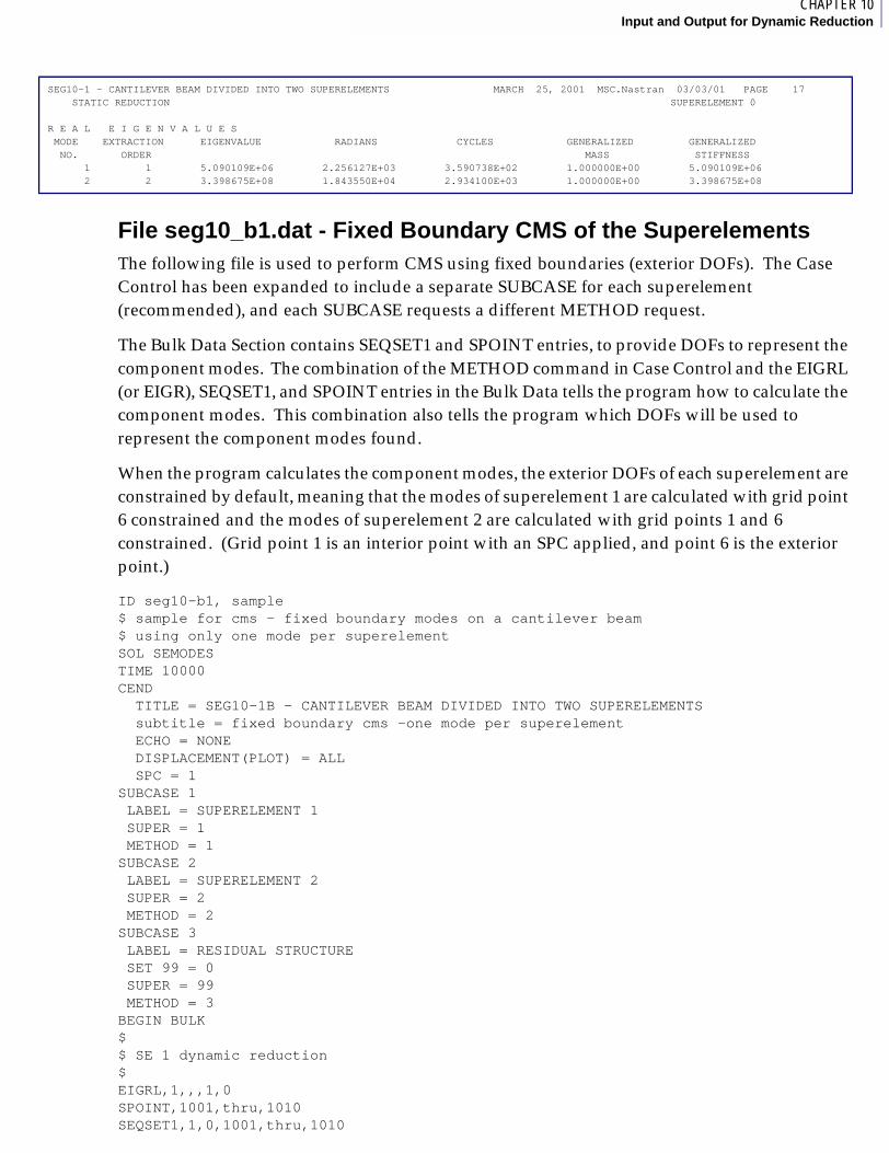
1CHAPTER 10Input and Output for Dynamic Reduction
File seg10_b1.dat - Fixed Boundary CMS of the SuperelementsThe following file is used to perform CMS using fixed boundaries (exterior DOFs). The Case Control has been expanded to include a separate SUBCASE for each superelement (recommended), and each SUBCASE requests a different METHOD request.
The Bulk Data Section contains SEQSET1 and SPOINT entries, to provide DOFs to represent the component modes. The combination of the METHOD command in Case Control and the EIGRL (or EIGR), SEQSET1, and SPOINT entries in the Bulk Data tells the program how to calculate the component modes. This combination also tells the program which DOFs will be used to represent the component modes found.
When the program calculates the component modes, the exterior DOFs of each superelement are constrained by default, meaning that the modes of superelement 1 are calculated with grid point 6 constrained and the modes of superelement 2 are calculated with grid points 1 and 6 constrained. (Grid point 1 is an interior point with an SPC applied, and point 6 is the exterior point.)
ID seg10-b1, sample$ sample for cms - fixed boundary modes on a cantilever beam$ using only one mode per superelementSOL SEMODESTIME 10000CEND TITLE = SEG10-1B - CANTILEVER BEAM DIVIDED INTO TWO SUPERELEMENTS subtitle = fixed boundary cms -one mode per superelement ECHO = NONE DISPLACEMENT(PLOT) = ALL SPC = 1SUBCASE 1 LABEL = SUPERELEMENT 1 SUPER = 1 METHOD = 1SUBCASE 2 LABEL = SUPERELEMENT 2 SUPER = 2 METHOD = 2SUBCASE 3 LABEL = RESIDUAL STRUCTURE SET 99 = 0 SUPER = 99 METHOD = 3BEGIN BULK$$ SE 1 dynamic reduction$EIGRL,1,,,1,0SPOINT,1001,thru,1010SEQSET1,1,0,1001,thru,1010
SEG10-1 - CANTILEVER BEAM DIVIDED INTO TWO SUPERELEMENTS MARCH 25, 2001 MSC.Nastran 03/03/01 PAGE 17 STATIC REDUCTION SUPERELEMENT 0 R E A L E I G E N V A L U E S MODE EXTRACTION EIGENVALUE RADIANS CYCLES GENERALIZED GENERALIZED NO. ORDER MASS STIFFNESS 1 1 5.090109E+06 2.256127E+03 3.590738E+02 1.000000E+00 5.090109E+06 2 2 3.398675E+08 1.843550E+04 2.934100E+03 1.000000E+00 3.398675E+08

$$ se 2 dynamic reduction$EIGRL,2,,,1,0spoint,2001,thru,2010seqset1,2,0,2001,thru,2010$$ residual structure$EIGRL,3,,,10,0$include ’cantbeam.dat’ENDDATA
This run calculates the fixed-boundary modes of each superelement, thus the output will include the eigenvalue summary table for each. Because this run has requests for only one mode per superelement, each superelement eigenvalue summary table has only one mode. The residual structure modes are improved over the static reduction case, but the modes are still not as accurate as we would like. Obtaining more modes for each superelement would improve the accuracy of the residual structure modes.
File seg10-c1 - Free-Free CMS of the superelementsThe next example shows how to use free-boundary CMS for a superelement. Note that the exterior points are not constrained during the calculation of the component modes. Any SPCs on interior points are included, and if there are any constraints on the exterior points, these constraints are applied physically at the downstream superelement that has them as interior points, not at the current superelement.
SEG10-1B - CANTILEVER BEAM DIVIDED INTO TWO SUPERELEMENTS MARCH 25, 2001 MSC.Nastran 03/03/01 PAGE 13 FIXED BOUNDARY CMS -ONE MODE PER SUPERELEMENT SUPERELEMENT 1 SUBCASE 1 R E A L E I G E N V A L U E SMODE EXTRACTION EIGENVALUE RADIANS CYCLES GENERALIZED GENERALIZED NO. ORDER MASS STIFFNESS 1 1 7.518384E+07 8.670861E+03 1.380010E+03 1.000000E+00 7.518384E+071
SEG10-1B - CANTILEVER BEAM DIVIDED INTO TWO SUPERELEMENTS MARCH 25, 2001 MSC.Nastran 03/03/01 PAGE 19 FIXED BOUNDARY CMS -ONE MODE PER SUPERELEMENT SUPERELEMENT 2 SUBCASE 2 R E A L E I G E N V A L U E SMODE EXTRACTION EIGENVALUE RADIANS CYCLES GENERALIZED GENERALIZED NO. ORDER MASS STIFFNESS 1 1 3.150545E+09 5.612971E+04 8.933320E+03 1.000000E+00 3.150545E+09
SEG10-1B - CANTILEVER BEAM DIVIDED INTO TWO SUPERELEMENTS MARCH 25, 2001 MSC.Nastran 03/03/01 PAGE 24 FIXED BOUNDARY CMS -ONE MODE PER SUPERELEMENT SUPERELEMENT 0 SUBCASE 3 R E A L E I G E N V A L U E SMODE EXTRACTION EIGENVALUE RADIANS CYCLES GENERALIZED GENERALIZED NO. ORDER MASS STIFFNESS 1 1 4.829352E+06 2.197579E+03 3.497555E+02 1.000000E+00 4.829352E+06 2 2 1.880461E+08 1.371299E+04 2.182490E+03 1.000000E+00 1.880461E+08 3 3 1.790023E+09 4.230867E+04 6.733633E+03 1.000000E+00 1.790023E+09 4 4 1.310846E+10 1.144922E+05 1.822200E+04 1.000000E+00 1.310846E+10.

1CHAPTER 10Input and Output for Dynamic Reduction
We will use the SECSET1 entry to specify that we want free-free CMS. This entry has an option to state that ALL exterior DOFs will be unconstrained during the calculation of the component modes; that option is displayed here. If only selected DOFs were set free during the calculation of the component modes, they would be listed on SECSET and/or SECSET1 entries.
Once again, in this example only one mode per superelement is requested. More modes are required for greater accuracy.
ID seg10-c1$ sample for cms - free boundary modes on a cantilever beam$ using only one mode per superelementSOL SEMODESTIME 10000CEND TITLE = SEG10-1B - CANTILEVER BEAM DIVIDED INTO TWO SUPERELEMENTS subtitle = free boundary cms -one mode per superelement ECHO = NONE DISPLACEMENT(PLOT) = ALL SPC = 1SUBCASE 1 LABEL = SUPERELEMENT 1 SUPER = 1 METHOD = 1SUBCASE 2 LABEL = SUPERELEMENT 2 SUPER = 2 METHOD = 2SUBCASE 3 LABEL = RESIDUAL STRUCTURE SET 99 = 0 SUPER = 99 METHOD = 3BEGIN BULK$$ SE 1 dynamic reduction$secset1,1,allEIGRL,1,,,1,0SPOINT,1001,thru,1010SEQSET1,1,0,1001,thru,1010$$ se 2 dynamic reduction$secset1,2,allEIGRL,2,,,1,0spoint,2001,thru,2010seqset1,2,0,2001,thru,2010$$ residual structure$EIGRL,3,,,10,0$include ’cantbeam.dat’ENDDATA
The results of the above run follow. The input file requests the calculation of only one mode per superelement. The resulting eigenvalue summary tables appear below. Superelement 1 is the tip of the beam and (when run with all exterior DOFs in the C-set) has rigid-body modes; the one mode found is one of those rigid-body modes. The filtering process finds that this rigid-body

mode is a linear combination of the static transformation vectors; this mode will be discarded. A better approach would be to list a lowest frequency of just above 0.0 hz on the EIGRL. Using this method, rigid-body modes would not be calculated.
Superelement 2 is the root of the beam, and interior point 1 is the point of fixity for the cantilever beam. Therefore, the expression free-free CMS does not really describe this superelement. The exterior grid point (GRID 6) is not constrained during the eigenvalue solution. However, interior grid point 1 has SPCs applied and is therefore constrained during the calculation of the modes. Thus, the component modes found for superelement 2 are the cantilevered modes of the component, which is shown in the eigenvalue summary table for superelement 2. The first mode has a natural frequency of 1,380 hz. Obviously, this mode is not a rigid-body mode and will be retained.
Notice that the frequencies are improved over the static reduction, but these frequencies are not as good as the fixed-boundary CMS results. There is no magic rule stating that free-free or fixed-boundary CMS are the best approaches for any model. You must use engineering judgement to determine which approach will provide component modes that best approximate the behavior of the superelement when it is attached to the rest of the model.
File seg10_d1.dat - Mixed Boundary CMSNow we will demonstrate mixed-boundary CMS. Superelement 1 is cantilevered from exterior grid point 6, thus fixed-boundary CMS is appropriate. That is, cantilevered modes represent how we expect this component to behave when it is attached to the rest of the structure. Superelement 2 also has exterior point 6; however, now it makes more sense to perform CMS with grid point 6 unconstrained. Fixed-boundary CMS does not represent how we expect this component to behave when it is attached to the rest of the model. Calculating the component modes with point 6 free (or cantilevered from interior grid point 1) gives a better representation. Thus, grid point 6 is placed in the C-set for superelement 2. These modes look more like we expect this component to behave when it is attached to the rest of the model.
SEG10-C1 - CANTILEVER BEAM DIVIDED INTO TWO SUPERELEMENTS MARCH 25, 2001 MSC.Nastran 03/03/01 PAGE 13 FREE BOUNDARY CMS -ONE MODE PER SUPERELEMENT SUPERELEMENT 1 SUBCASE 1
R E A L E I G E N V A L U E S MODE EXTRACTION EIGENVALUE RADIANS CYCLES GENERALIZED GENERALIZED NO. ORDER MASS STIFFNESS 1 1 1.123603E-05 3.352019E-03 5.334903E-04 1.000000E+00 1.123603E-051
SEG10-C1 - CANTILEVER BEAM DIVIDED INTO TWO SUPERELEMENTS MARCH 25, 2001 MSC.Nastran 03/03/01 PAGE 19 FREE BOUNDARY CMS -ONE MODE PER SUPERELEMENT SUPERELEMENT 2 SUBCASE 2
R E A L E I G E N V A L U E S MODE EXTRACTION EIGENVALUE RADIANS CYCLES GENERALIZED GENERALIZED NO. ORDER MASS STIFFNESS 1 1 7.518384E+07 8.670861E+03 1.380010E+03 1.000000E+00 7.518384E+071
SEG10-C1 - CANTILEVER BEAM DIVIDED INTO TWO SUPERELEMENTS MARCH 25, 2001 MSC.Nastran 03/03/01 PAGE 24FREE BOUNDARY CMS -ONE MODE PER SUPERELEMENT SUPERELEMENT 0 SUBCASE 3
R E A L E I G E N V A L U E S MODE EXTRACTION EIGENVALUE RADIANS CYCLES GENERALIZED GENERALIZED NO. ORDER MASS STIFFNESS 1 1 5.089954E+06 2.256093E+03 3.590683E+02 1.000000E+00 5.089954E+06 2 2 3.258532E+08 1.805140E+04 2.872970E+03 1.000000E+00 3.258532E+08 3 3 6.048577E+09 7.777260E+04 1.237789E+04 1.000000E+00 6.048577E+09
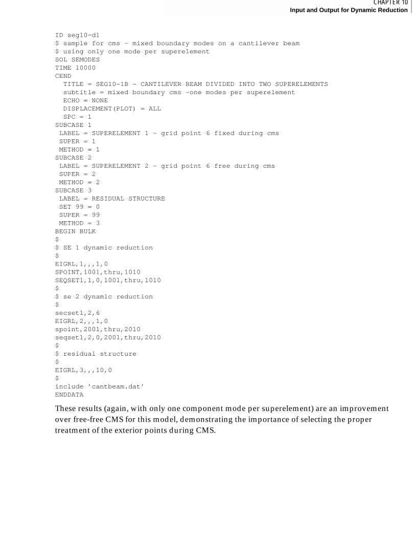
1CHAPTER 10Input and Output for Dynamic Reduction
ID seg10-d1$ sample for cms - mixed boundary modes on a cantilever beam$ using only one mode per superelementSOL SEMODESTIME 10000CEND TITLE = SEG10-1B - CANTILEVER BEAM DIVIDED INTO TWO SUPERELEMENTS subtitle = mixed boundary cms -one modes per superelement ECHO = NONE DISPLACEMENT(PLOT) = ALL SPC = 1SUBCASE 1 LABEL = SUPERELEMENT 1 - grid point 6 fixed during cms SUPER = 1 METHOD = 1SUBCASE 2 LABEL = SUPERELEMENT 2 - grid point 6 free during cms SUPER = 2 METHOD = 2SUBCASE 3 LABEL = RESIDUAL STRUCTURE SET 99 = 0 SUPER = 99 METHOD = 3BEGIN BULK$$ SE 1 dynamic reduction$EIGRL,1,,,1,0SPOINT,1001,thru,1010SEQSET1,1,0,1001,thru,1010$$ se 2 dynamic reduction$secset1,2,6EIGRL,2,,,1,0spoint,2001,thru,2010seqset1,2,0,2001,thru,2010$$ residual structure$EIGRL,3,,,10,0$include ’cantbeam.dat’ENDDATA
These results (again, with only one component mode per superelement) are an improvement over free-free CMS for this model, demonstrating the importance of selecting the proper treatment of the exterior points during CMS.
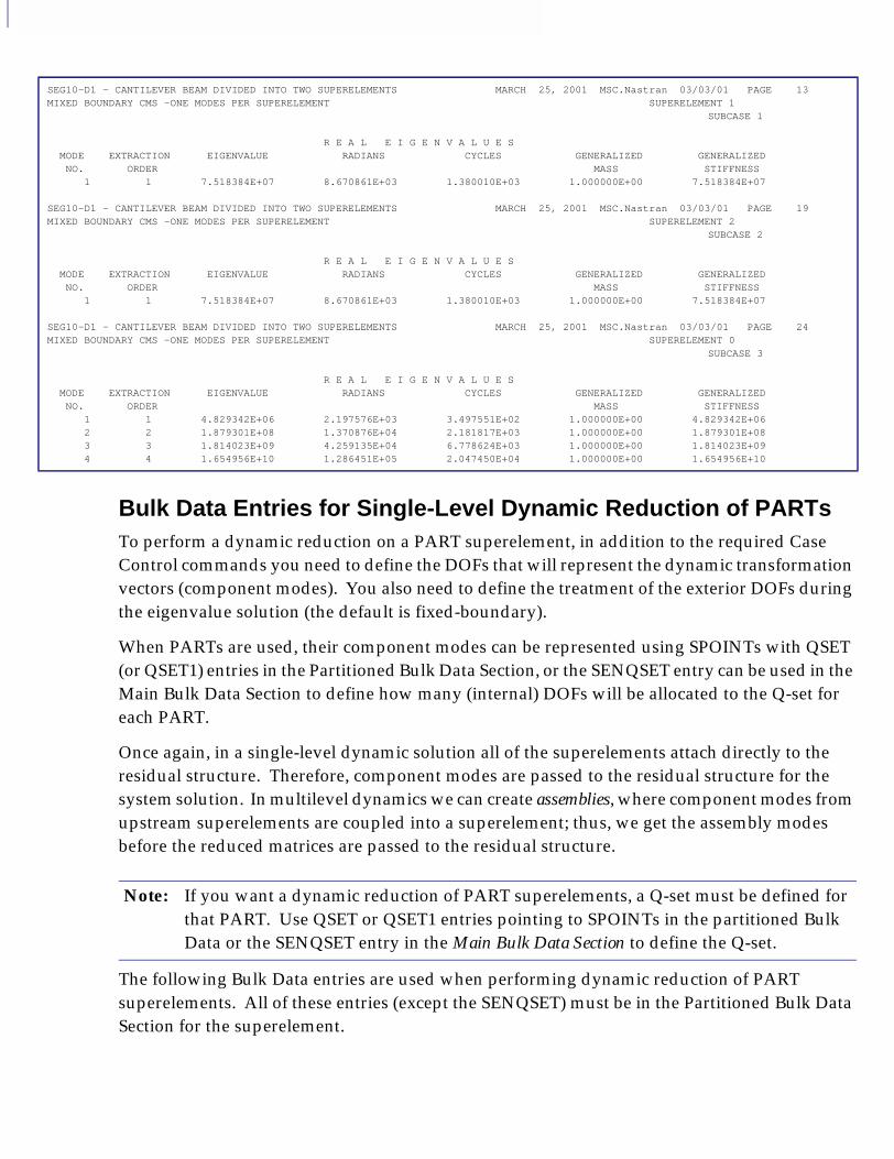
Bulk Data Entries for Single-Level Dynamic Reduction of PARTsTo perform a dynamic reduction on a PART superelement, in addition to the required Case Control commands you need to define the DOFs that will represent the dynamic transformation vectors (component modes). You also need to define the treatment of the exterior DOFs during the eigenvalue solution (the default is fixed-boundary).
When PARTs are used, their component modes can be represented using SPOINTs with QSET (or QSET1) entries in the Partitioned Bulk Data Section, or the SENQSET entry can be used in the Main Bulk Data Section to define how many (internal) DOFs will be allocated to the Q-set for each PART.
Once again, in a single-level dynamic solution all of the superelements attach directly to the residual structure. Therefore, component modes are passed to the residual structure for the system solution. In multilevel dynamics we can create assemblies, where component modes from upstream superelements are coupled into a superelement; thus, we get the assembly modes before the reduced matrices are passed to the residual structure.
The following Bulk Data entries are used when performing dynamic reduction of PART superelements. All of these entries (except the SENQSET) must be in the Partitioned Bulk Data Section for the superelement.
SEG10-D1 - CANTILEVER BEAM DIVIDED INTO TWO SUPERELEMENTS MARCH 25, 2001 MSC.Nastran 03/03/01 PAGE 13MIXED BOUNDARY CMS -ONE MODES PER SUPERELEMENT SUPERELEMENT 1 SUBCASE 1
R E A L E I G E N V A L U E S MODE EXTRACTION EIGENVALUE RADIANS CYCLES GENERALIZED GENERALIZED NO. ORDER MASS STIFFNESS 1 1 7.518384E+07 8.670861E+03 1.380010E+03 1.000000E+00 7.518384E+07
SEG10-D1 - CANTILEVER BEAM DIVIDED INTO TWO SUPERELEMENTS MARCH 25, 2001 MSC.Nastran 03/03/01 PAGE 19MIXED BOUNDARY CMS -ONE MODES PER SUPERELEMENT SUPERELEMENT 2 SUBCASE 2
R E A L E I G E N V A L U E S MODE EXTRACTION EIGENVALUE RADIANS CYCLES GENERALIZED GENERALIZED NO. ORDER MASS STIFFNESS 1 1 7.518384E+07 8.670861E+03 1.380010E+03 1.000000E+00 7.518384E+07
SEG10-D1 - CANTILEVER BEAM DIVIDED INTO TWO SUPERELEMENTS MARCH 25, 2001 MSC.Nastran 03/03/01 PAGE 24 MIXED BOUNDARY CMS -ONE MODES PER SUPERELEMENT SUPERELEMENT 0 SUBCASE 3
R E A L E I G E N V A L U E S MODE EXTRACTION EIGENVALUE RADIANS CYCLES GENERALIZED GENERALIZED NO. ORDER MASS STIFFNESS 1 1 4.829342E+06 2.197576E+03 3.497551E+02 1.000000E+00 4.829342E+06 2 2 1.879301E+08 1.370876E+04 2.181817E+03 1.000000E+00 1.879301E+08 3 3 1.814023E+09 4.259135E+04 6.778624E+03 1.000000E+00 1.814023E+09 4 4 1.654956E+10 1.286451E+05 2.047450E+04 1.000000E+00 1.654956E+10
Note: If you want a dynamic reduction of PART superelements, a Q-set must be defined for that PART. Use QSET or QSET1 entries pointing to SPOINTs in the partitioned Bulk Data or the SENQSET entry in the Main Bulk Data Section to define the Q-set.

1CHAPTER 10Input and Output for Dynamic Reduction
For PART superelements, component modes must be attached to SPOINTs. (An exception to this rule does exist-you can use the SENQSET entry to create internal DOFs to represent the dynamic vectors). If SENQSET entries are used, internal DOFs are created and show up in the Superelement Connectivity List. These internal DOFs have a number range well above the user-accessible range of grid or SPOINT ids. That is, the DOFs representing the dynamic vectors exist and are included in the solution, but you are unable to exercise any control over their use in the solution. To exercise control over the DOFs representing the dynamic vectors (for example,
QSET and/or QSET1 one or both or these entries can be used to define the DOFs that will be used to represent the superelement dynamic transformation vectors (component modes) in subsequent processing; these entries point to SPOINTs. When PARTs exist in a model, grid points cannot be used for the Q-set. (Note: If you use the SENQSET, this entry is not required)
BSET and/or BSET1 list of exterior DOFs that will be constrained during the calculation of the dynamic transformation. (Default = all exterior DOFs.) Any DOFs listed on a BSET or BSET1 entry will become exterior DOFs even if not selected by a SECONCT entry, automatic attachment, or ASET and/or ASET1 entries.
Note: For PARTs superelements, for each DOF listed on SUPORT entries, one dynamic transformation vector (starting with the lowest natural frequency) is removed. Because the program does not perform checking, we do not recommend this approach.
CSET and/or CSET1 list of exterior DOFs that will not be constrained during the calculation of the dynamic transformation vectors. (Default = none.) Any DOFs listed on a CSET or CSET1 entry will become an exterior DOFs even if not selected by a SECONCT entry, automatic attachment, or ASET and/or ASET1 entries.
SUPORT list of exterior DOFs that are to be placed into the superelement R-set. These DOFs are not constrained during the calculation of the dynamic transformation vectors; however, for each DOF listed on the SUPORT entry, one dynamic transformation vector is removed without any checking performed.
SENQSET list of the number of automatically generated Q-set DOFs for selected superelements or all superelements. This entry can be used only if there are one or more PARTs in the deck. If used, this entry automatically generates internal DOFs for the Q-set for the selected superelements. These DOFs are passed to the residual structure with no coupling to downstream superelements until the residual structure is processed; therefore, this entry may not be the best choice for multilevel dynamic analysis.
SPOINT You must define the degrees of freedom MSC.Nastran will use for the component modes. (Note: If you use the SENQSET, this entry is not required).
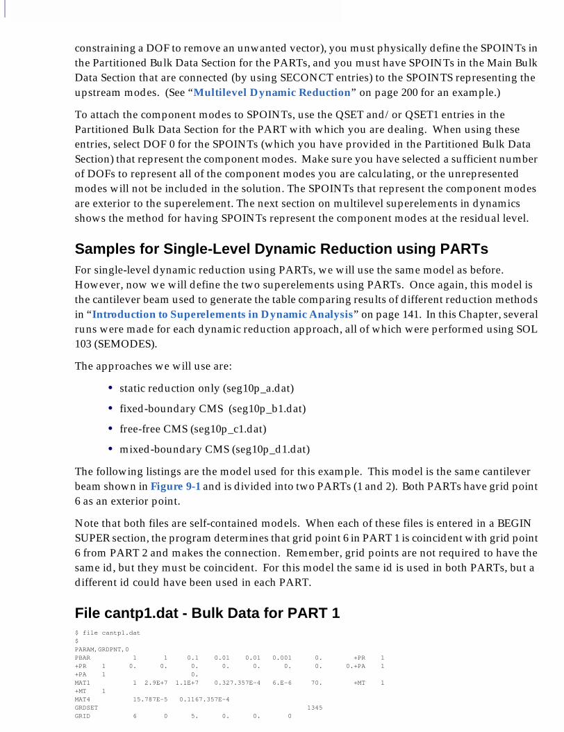
constraining a DOF to remove an unwanted vector), you must physically define the SPOINTs in the Partitioned Bulk Data Section for the PARTs, and you must have SPOINTs in the Main Bulk Data Section that are connected (by using SECONCT entries) to the SPOINTS representing the upstream modes. (See “Multilevel Dynamic Reduction” on page 200 for an example.)
To attach the component modes to SPOINTs, use the QSET and/or QSET1 entries in the Partitioned Bulk Data Section for the PART with which you are dealing. When using these entries, select DOF 0 for the SPOINTs (which you have provided in the Partitioned Bulk Data Section) that represent the component modes. Make sure you have selected a sufficient number of DOFs to represent all of the component modes you are calculating, or the unrepresented modes will not be included in the solution. The SPOINTs that represent the component modes are exterior to the superelement. The next section on multilevel superelements in dynamics shows the method for having SPOINTs represent the component modes at the residual level.
Samples for Single-Level Dynamic Reduction using PARTsFor single-level dynamic reduction using PARTs, we will use the same model as before. However, now we will define the two superelements using PARTs. Once again, this model is the cantilever beam used to generate the table comparing results of different reduction methods in “Introduction to Superelements in Dynamic Analysis” on page 141. In this Chapter, several runs were made for each dynamic reduction approach, all of which were performed using SOL 103 (SEMODES).
The approaches we will use are:
• static reduction only (seg10p_a.dat)
• fixed-boundary CMS (seg10p_b1.dat)
• free-free CMS (seg10p_c1.dat)
• mixed-boundary CMS (seg10p_d1.dat)
The following listings are the model used for this example. This model is the same cantilever beam shown in Figure 9-1 and is divided into two PARTs (1 and 2). Both PARTs have grid point 6 as an exterior point.
Note that both files are self-contained models. When each of these files is entered in a BEGIN SUPER section, the program determines that grid point 6 in PART 1 is coincident with grid point 6 from PART 2 and makes the connection. Remember, grid points are not required to have the same id, but they must be coincident. For this model the same id is used in both PARTs, but a different id could have been used in each PART.
File cantp1.dat - Bulk Data for PART 1$ file cantp1.dat$PARAM,GRDPNT,0PBAR 1 1 0.1 0.01 0.01 0.001 0. +PR 1+PR 1 0. 0. 0. 0. 0. 0. 0. 0.+PA 1+PA 1 0.MAT1 1 2.9E+7 1.1E+7 0.327.357E-4 6.E-6 70. +MT 1+MT 1 MAT4 15.787E-5 0.1167.357E-4GRDSET 1345GRID 6 0 5. 0. 0. 0
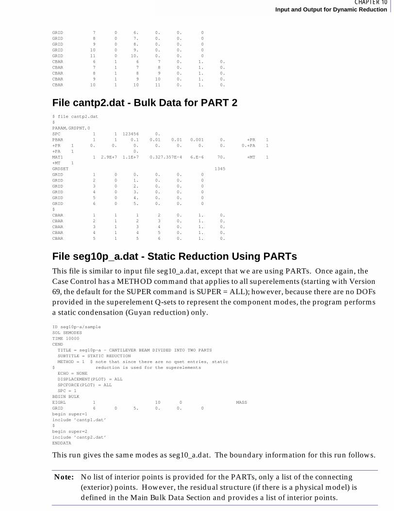
1CHAPTER 10Input and Output for Dynamic Reduction
GRID 7 0 6. 0. 0. 0 GRID 8 0 7. 0. 0. 0 GRID 9 0 8. 0. 0. 0 GRID 10 0 9. 0. 0. 0 GRID 11 0 10. 0. 0. 0 CBAR 6 1 6 7 0. 1. 0.CBAR 7 1 7 8 0. 1. 0.CBAR 8 1 8 9 0. 1. 0.CBAR 9 1 9 10 0. 1. 0.CBAR 10 1 10 11 0. 1. 0.
File cantp2.dat - Bulk Data for PART 2$ file cantp2.dat $PARAM,GRDPNT,0SPC 1 1 123456 0.PBAR 1 1 0.1 0.01 0.01 0.001 0. +PR 1+PR 1 0. 0. 0. 0. 0. 0. 0. 0.+PA 1+PA 1 0.MAT1 1 2.9E+7 1.1E+7 0.327.357E-4 6.E-6 70. +MT 1+MT 1 GRDSET 1345GRID 1 0 0. 0. 0. 0 GRID 2 0 1. 0. 0. 0 GRID 3 0 2. 0. 0. 0 GRID 4 0 3. 0. 0. 0 GRID 5 0 4. 0. 0. 0 GRID 6 0 5. 0. 0. 0 $CBAR 1 1 1 2 0. 1. 0.CBAR 2 1 2 3 0. 1. 0.CBAR 3 1 3 4 0. 1. 0.CBAR 4 1 4 5 0. 1. 0.CBAR 5 1 5 6 0. 1. 0.
File seg10p_a.dat - Static Reduction Using PARTsThis file is similar to input file seg10_a.dat, except that we are using PARTs. Once again, the Case Control has a METHOD command that applies to all superelements (starting with Version 69, the default for the SUPER command is SUPER = ALL); however, because there are no DOFs provided in the superelement Q-sets to represent the component modes, the program performs a static condensation (Guyan reduction) only.
ID seg10p-a/sample SOL SEMODESTIME 10000CEND TITLE = seg10p-a - CANTILEVER BEAM DIVIDED INTO TWO PARTS SUBTITLE = STATIC REDUCTION METHOD = 1 $ note that since there are no qset entries, static$ reduction is used for the superelements ECHO = NONE DISPLACEMENT(PLOT) = ALL SPCFORCE(PLOT) = ALL SPC = 1BEGIN BULKEIGRL 1 10 0 MASSGRID 6 0 5. 0. 0. 0begin super=1include ’cantp1.dat’$begin super=2include ’cantp2.dat’ENDDATA
This run gives the same modes as seg10_a.dat. The boundary information for this run follows.
Note: No list of interior points is provided for the PARTs, only a list of the connecting (exterior) points. However, the residual structure (if there is a physical model) is defined in the Main Bulk Data Section and provides a list of interior points.
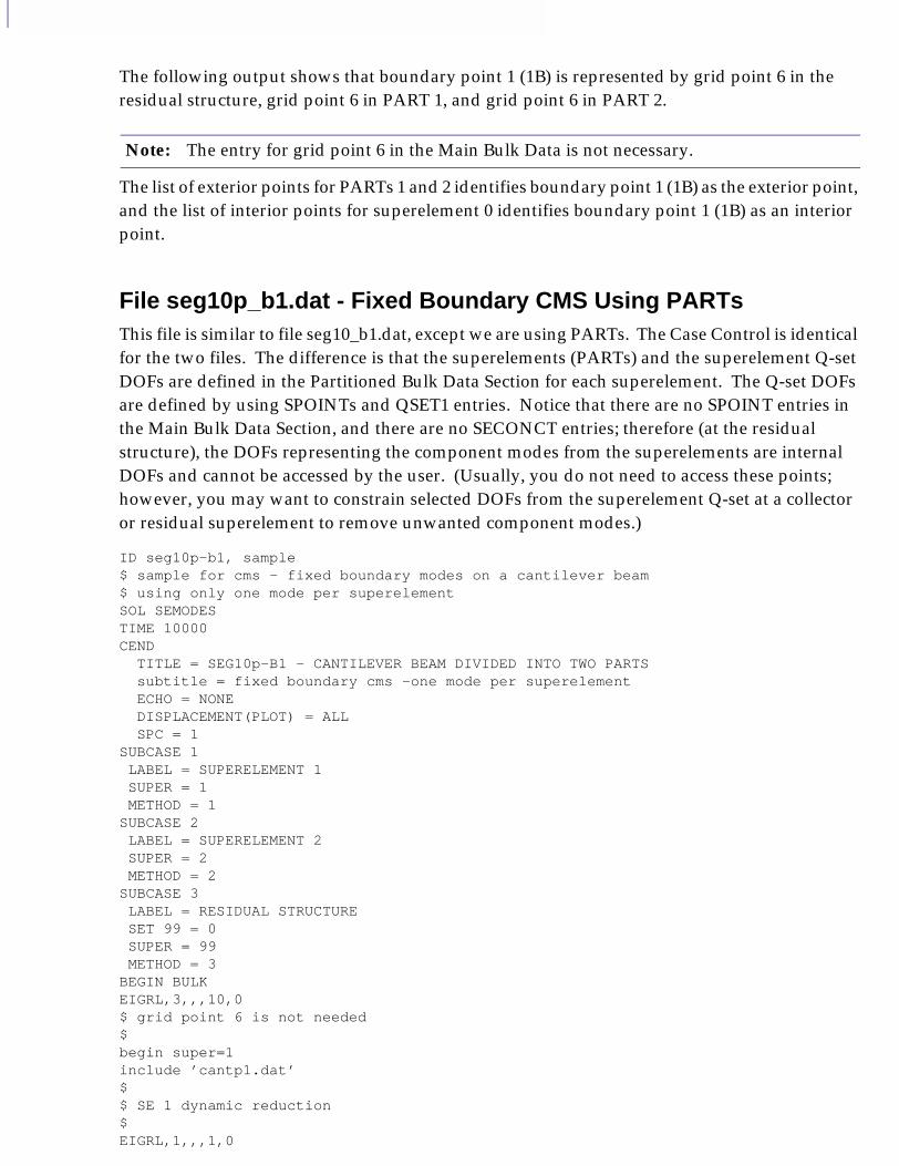
The following output shows that boundary point 1 (1B) is represented by grid point 6 in the residual structure, grid point 6 in PART 1, and grid point 6 in PART 2.
The list of exterior points for PARTs 1 and 2 identifies boundary point 1 (1B) as the exterior point, and the list of interior points for superelement 0 identifies boundary point 1 (1B) as an interior point.
File seg10p_b1.dat - Fixed Boundary CMS Using PARTsThis file is similar to file seg10_b1.dat, except we are using PARTs. The Case Control is identical for the two files. The difference is that the superelements (PARTs) and the superelement Q-set DOFs are defined in the Partitioned Bulk Data Section for each superelement. The Q-set DOFs are defined by using SPOINTs and QSET1 entries. Notice that there are no SPOINT entries in the Main Bulk Data Section, and there are no SECONCT entries; therefore (at the residual structure), the DOFs representing the component modes from the superelements are internal DOFs and cannot be accessed by the user. (Usually, you do not need to access these points; however, you may want to constrain selected DOFs from the superelement Q-set at a collector or residual superelement to remove unwanted component modes.)
ID seg10p-b1, sample$ sample for cms - fixed boundary modes on a cantilever beam$ using only one mode per superelementSOL SEMODESTIME 10000CEND TITLE = SEG10p-B1 - CANTILEVER BEAM DIVIDED INTO TWO PARTS subtitle = fixed boundary cms -one mode per superelement ECHO = NONE DISPLACEMENT(PLOT) = ALL SPC = 1SUBCASE 1 LABEL = SUPERELEMENT 1 SUPER = 1 METHOD = 1SUBCASE 2 LABEL = SUPERELEMENT 2 SUPER = 2 METHOD = 2SUBCASE 3 LABEL = RESIDUAL STRUCTURE SET 99 = 0 SUPER = 99 METHOD = 3BEGIN BULKEIGRL,3,,,10,0$ grid point 6 is not needed$begin super=1include ’cantp1.dat’$$ SE 1 dynamic reduction$EIGRL,1,,,1,0
Note: The entry for grid point 6 in the Main Bulk Data is not necessary.

1CHAPTER 10Input and Output for Dynamic Reduction
SPOINT,1001,thru,1010QSET1,0,1001,thru,1010$begin super=2include ’cantp2.dat’$$ se 2 dynamic reduction$EIGRL,2,,,1,0spoint,2001,thru,2010qset1,0,2001,thru,2010$ENDDATA
Once again, this is the same structure as that used in example seg10-b1, which results in the same modes; however, the components are now defined as PARTs and are automatically connected to each other. Also, there is no physical residual structure model; rather, the residual structure consists of internal DOFs created to represent the DOFs passed down from the upstream superelements.
The following example shows the boundary point lists. Notice that the SPOINTs used for the modes are identified as 1B through 10B (superelement 1) and 12B through 21B (superelement 2). Boundary point 11B is used to identify exterior grid point 6 in superelements 1 and 2. Because no equivalent grid point exists in the residual structure, boundary point 11B is represented by internal DOF that are not accessible to the user. These DOF are, however, included in the solution. No model is provided for the residual structure in this example; the residual structure consists only of copies of the boundary points from the upstream superelements and their component modes.
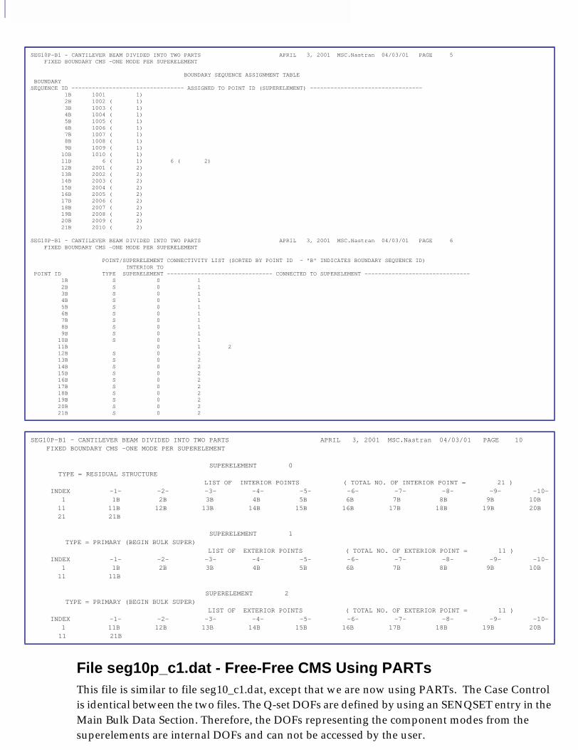
File seg10p_c1.dat - Free-Free CMS Using PARTsThis file is similar to file seg10_c1.dat, except that we are now using PARTs. The Case Control is identical between the two files. The Q-set DOFs are defined by using an SENQSET entry in the Main Bulk Data Section. Therefore, the DOFs representing the component modes from the superelements are internal DOFs and can not be accessed by the user.
SEG10P-B1 - CANTILEVER BEAM DIVIDED INTO TWO PARTS APRIL 3, 2001 MSC.Nastran 04/03/01 PAGE 5 FIXED BOUNDARY CMS -ONE MODE PER SUPERELEMENT BOUNDARY SEQUENCE ASSIGNMENT TABLE BOUNDARYSEQUENCE ID --------------------------------- ASSIGNED TO POINT ID (SUPERELEMENT) --------------------------------- 1B 1001 1) 2B 1002 ( 1) 3B 1003 ( 1) 4B 1004 ( 1) 5B 1005 ( 1) 6B 1006 ( 1) 7B 1007 ( 1) 8B 1008 ( 1) 9B 1009 ( 1) 10B 1010 ( 1) 11B 6 ( 1) 6 ( 2) 12B 2001 ( 2) 13B 2002 ( 2) 14B 2003 ( 2) 15B 2004 ( 2) 16B 2005 ( 2) 17B 2006 ( 2) 18B 2007 ( 2) 19B 2008 ( 2) 20B 2009 ( 2) 21B 2010 ( 2)
SEG10P-B1 - CANTILEVER BEAM DIVIDED INTO TWO PARTS APRIL 3, 2001 MSC.Nastran 04/03/01 PAGE 6 FIXED BOUNDARY CMS -ONE MODE PER SUPERELEMENT POINT/SUPERELEMENT CONNECTIVITY LIST (SORTED BY POINT ID - "B" INDICATES BOUNDARY SEQUENCE ID) INTERIOR TO POINT ID TYPE SUPERELEMENT ------------------------------- CONNECTED TO SUPERELEMENT ------------------------------- 1B S 0 1 2B S 0 1 3B S 0 1 4B S 0 1 5B S 0 1 6B S 0 1 7B S 0 1 8B S 0 1 9B S 0 1 10B S 0 1 11B 0 1 2 12B S 0 2 13B S 0 2 14B S 0 2 15B S 0 2 16B S 0 2 17B S 0 2 18B S 0 2 19B S 0 2 20B S 0 2 21B S 0 2
SEG10P-B1 - CANTILEVER BEAM DIVIDED INTO TWO PARTS APRIL 3, 2001 MSC.Nastran 04/03/01 PAGE 10 FIXED BOUNDARY CMS -ONE MODE PER SUPERELEMENT SUPERELEMENT 0 TYPE = RESIDUAL STRUCTURE LIST OF INTERIOR POINTS ( TOTAL NO. OF INTERIOR POINT = 21 ) INDEX -1- -2- -3- -4- -5- -6- -7- -8- -9- -10- 1 1B 2B 3B 4B 5B 6B 7B 8B 9B 10B 11 11B 12B 13B 14B 15B 16B 17B 18B 19B 20B 21 21B
SUPERELEMENT 1 TYPE = PRIMARY (BEGIN BULK SUPER) LIST OF EXTERIOR POINTS ( TOTAL NO. OF EXTERIOR POINT = 11 ) INDEX -1- -2- -3- -4- -5- -6- -7- -8- -9- -10- 1 1B 2B 3B 4B 5B 6B 7B 8B 9B 10B 11 11B
SUPERELEMENT 2 TYPE = PRIMARY (BEGIN BULK SUPER) LIST OF EXTERIOR POINTS ( TOTAL NO. OF EXTERIOR POINT = 11 ) INDEX -1- -2- -3- -4- -5- -6- -7- -8- -9- -10- 1 11B 12B 13B 14B 15B 16B 17B 18B 19B 20B 11 21B

1CHAPTER 10Input and Output for Dynamic Reduction
To perform free-free CMS, we use CSET1 (you can also use CSET entries) entries in the Partitioned Bulk Data Section for each PART. Any exterior DOFs that we do not want to constrain during the calculation of the component modes must be listed on CSET, CSET1, or SUPORT entries in the Partitioned Bulk Data Section for that PART.
Because we have asked the program to calculate the 0.0 hz modes of each PART, we are depending on the logic in the program to eliminate these modes. We could use SUPORT entries on selected exterior DOFs for the PARTs. For each exterior DOF defined on a SUPORT entry for a PART, one mode of the component is discarded, which is similar to the SESUP entry for main Bulk Data superelements. When calculating the modes of the PARTs, any exterior DOFs that are listed on CSET, CSET1, or SUPORT entries will not be constrained. Because there is a CSET1 entry in each Partitioned Bulk Data Section, the PARTs component modes are caculated with grid point 6 unconstrained, thus providing free-free modes for PART 1 and cantilevered modes for PART 2.
This sample demonstrates the use of the SENQSET entry. In the Main Bulk Data Section, we have asked that 10 internal DOFs be created to represent the component modes of each superelement in this model.
ID seg10p-c1$ sample for cms - free boundary modes on a cantilever beam$ using only one mode per superelementSOL SEMODESCEND TITLE = SEG10P-C1 - CANTILEVER BEAM DIVIDED INTO TWO PARTS subtitle = free boundary cms -one mode per superelement ECHO = NONE DISPLACEMENT(PLOT) = ALL SPC = 1SUBCASE 1 LABEL = SUPELEMENT 1 SUPER = 1 METHOD = 1SUBCASE 2 LABEL = SUPERELEMENT 2 SUPER = 2 METHOD = 2SUBCASE 3 LABEL = RESIDUAL STRUCTURE SET 99 = 0 SUPER = 99 METHOD = 3BEGIN BULKEIGRL,3,,,10,0$$ show use of SENQSET$senqset,all,10$begin super = 1include ’cantp1.dat’$$ SE 1 dynamic reduction$cset1,123456,6EIGRL,1,,,1,0$

begin super=2include ’cantp2.dat’$$ se 2 dynamic reduction$cset1,123456,6EIGRL,2,,,1,0$ENDDATA
The results of this run duplicate those in example seg10-c1. As in the previous example, there is no physical residual structure model, rather the residual structure consists of internal DOFs created to represent the DOFs passed down from the upstream superelements.
The following output shows the boundary point lists. The Boundary Sequence Assignment Table (Figure 10-2) finds grid point 6 in both superelements 1 and 2 coincident and identifies these points as point 1B. The next output shows all connecting points for the superelements. Notice that the internal DOFs created by the SENQSET entry are identified as 147477001B through 147477010B for superelement 2 and 147480001B through 147480010B for superelement 1. These numbers are outside of the range for defining grid or SPOINT entries and are not accessible to any input entries in MSC.Nastran. These numbers are internal DOFs generated solely to represent the component modes of the two superelements.
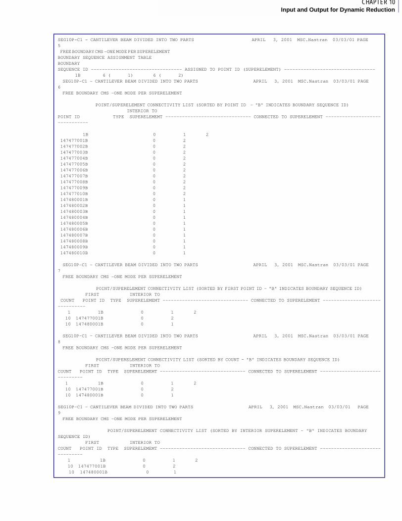
1CHAPTER 10Input and Output for Dynamic Reduction
SEG10P-C1 - CANTILEVER BEAM DIVIDED INTO TWO PARTS APRIL 3, 2001 MSC.Nastran 03/03/01 PAGE 5 FREE BOUNDARY CMS -ONE MODE PER SUPERELEMENT BOUNDARY SEQUENCE ASSIGNMENT TABLEBOUNDARYSEQUENCE ID --------------------------------- ASSIGNED TO POINT ID (SUPERELEMENT) --------------------------------- 1B 6 ( 1) 6 ( 2) SEG10P-C1 - CANTILEVER BEAM DIVIDED INTO TWO PARTS APRIL 3, 2001 MSC.Nastran 03/03/01 PAGE 6 FREE BOUNDARY CMS -ONE MODE PER SUPERELEMENT POINT/SUPERELEMENT CONNECTIVITY LIST (SORTED BY POINT ID - "B" INDICATES BOUNDARY SEQUENCE ID) INTERIOR TOPOINT ID TYPE SUPERELEMEMT ------------------------------- CONNECTED TO SUPERELEMENT -------------------------------
1B 0 1 2 147477001B 0 2 147477002B 0 2 147477003B 0 2 147477004B 0 2 147477005B 0 2 147477006B 0 2 147477007B 0 2 147477008B 0 2 147477009B 0 2 147477010B 0 2 147480001B 0 1 147480002B 0 1 147480003B 0 1 147480004B 0 1 147480005B 0 1 147480006B 0 1 147480007B 0 1 147480008B 0 1 147480009B 0 1 147480010B 0 1
SEG10P-C1 - CANTILEVER BEAM DIVIDED INTO TWO PARTS APRIL 3, 2001 MSC.Nastran 03/03/01 PAGE 7 FREE BOUNDARY CMS -ONE MODE PER SUPERELEMENT POINT/SUPERELEMENT CONNECTIVITY LIST (SORTED BY FIRST POINT ID - "B" INDICATES BOUNDARY SEQUENCE ID) FIRST INTERIOR TO COUNT POINT ID TYPE SUPERELEMEMT ------------------------------- CONNECTED TO SUPERELEMENT ------------------------------- 1 1B 0 1 2 10 147477001B 0 2 10 147480001B 0 1
SEG10P-C1 - CANTILEVER BEAM DIVIDED INTO TWO PARTS APRIL 3, 2001 MSC.Nastran 03/03/01 PAGE 8 FREE BOUNDARY CMS -ONE MODE PER SUPERELEMENT POINT/SUPERELEMENT CONNECTIVITY LIST (SORTED BY COUNT - "B" INDICATES BOUNDARY SEQUENCE ID) FIRST INTERIOR TOCOUNT POINT ID TYPE SUPERELEMEMT ------------------------------- CONNECTED TO SUPERELEMENT ------------------------------- 1 1B 0 1 2 10 147477001B 0 2 10 147480001B 0 1
SEG10P-C1 - CANTILEVER BEAM DIVIDED INTO TWO PARTS APRIL 3, 2001 MSC.Nastran 03/03/01 PAGE 9 FREE BOUNDARY CMS -ONE MODE PER SUPERELEMENT POINT/SUPERELEMENT CONNECTIVITY LIST (SORTED BY INTERIOR SUPERELEMENT - "B" INDICATES BOUNDARY SEQUENCE ID) FIRST INTERIOR TOCOUNT POINT ID TYPE SUPERELEMEMT ------------------------------- CONNECTED TO SUPERELEMENT ------------------------------- 1 1B 0 1 2 10 147477001B 0 2 10 147480001B 0 1
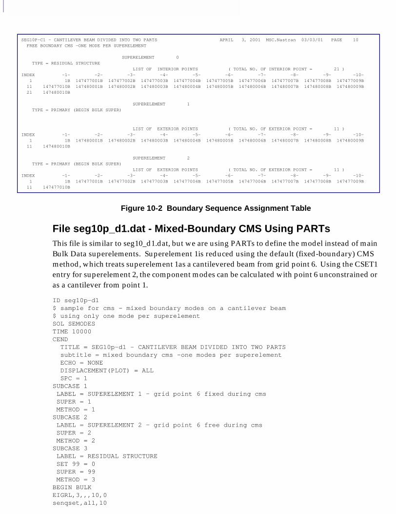
Figure 10-2 Boundary Sequence Assignment Table
File seg10p_d1.dat - Mixed-Boundary CMS Using PARTsThis file is similar to seg10_d1.dat, but we are using PARTs to define the model instead of main Bulk Data superelements. Superelement 1is reduced using the default (fixed-boundary) CMS method, which treats superelement 1as a cantilevered beam from grid point 6. Using the CSET1 entry for superelement 2, the component modes can be calculated with point 6 unconstrained or as a cantilever from point 1.
ID seg10p-d1$ sample for cms - mixed boundary modes on a cantilever beam$ using only one mode per superelementSOL SEMODESTIME 10000CEND TITLE = SEG10p-d1 - CANTILEVER BEAM DIVIDED INTO TWO PARTS subtitle = mixed boundary cms -one modes per superelement ECHO = NONE DISPLACEMENT(PLOT) = ALL SPC = 1SUBCASE 1 LABEL = SUPERELEMENT 1 - grid point 6 fixed during cms SUPER = 1 METHOD = 1SUBCASE 2 LABEL = SUPERELEMENT 2 - grid point 6 free during cms SUPER = 2 METHOD = 2SUBCASE 3 LABEL = RESIDUAL STRUCTURE SET 99 = 0 SUPER = 99 METHOD = 3BEGIN BULKEIGRL,3,,,10,0senqset,all,10
SEG10P-C1 - CANTILEVER BEAM DIVIDED INTO TWO PARTS APRIL 3, 2001 MSC.Nastran 03/03/01 PAGE 10 FREE BOUNDARY CMS -ONE MODE PER SUPERELEMENT SUPERELEMENT 0 TYPE = RESIDUAL STRUCTURE LIST OF INTERIOR POINTS ( TOTAL NO. OF INTERIOR POINT = 21 ) INDEX -1- -2- -3- -4- -5- -6- -7- -8- -9- -10- 1 1B 147477001B 147477002B 147477003B 147477004B 147477005B 147477006B 147477007B 147477008B 147477009B 11 147477010B 147480001B 147480002B 147480003B 147480004B 147480005B 147480006B 147480007B 147480008B 147480009B 21 147480010B
SUPERELEMENT 1 TYPE = PRIMARY (BEGIN BULK SUPER)
LIST OF EXTERIOR POINTS ( TOTAL NO. OF EXTERIOR POINT = 11 ) INDEX -1- -2- -3- -4- -5- -6- -7- -8- -9- -10- 1 1B 147480001B 147480002B 147480003B 147480004B 147480005B 147480006B 147480007B 147480008B 147480009B 11 147480010B
SUPERELEMENT 2 TYPE = PRIMARY (BEGIN BULK SUPER) LIST OF EXTERIOR POINTS ( TOTAL NO. OF EXTERIOR POINT = 11 ) INDEX -1- -2- -3- -4- -5- -6- -7- -8- -9- -10- 1 1B 147477001B 147477002B 147477003B 147477004B 147477005B 147477006B 147477007B 147477008B 147477009B 11 147477010B

1CHAPTER 10Input and Output for Dynamic Reduction
$begin super=1include ’cantp1.dat’$$ SE 1 dynamic reduction$EIGRL,1,,,1,0$begin super=2include ’cantp2.dat’$$ se 2 dynamic reduction$cset1,123456,6EIGRL,2,,,1,0$ENDDATA
The results of this problem are identical to the results for seg10-d1. No additional discussion is needed here.
10.3 Multilevel Dynamic ReductionMultilevel dynamic reduction is desirable for many models, though not required. As in static analysis, using a multilevel reduction reduces the size of the residual structure (resulting in a faster solution time for model change restarts). However, in dynamic analysis multilevel reduction can be used to determine how assemblies perform before looking at the full structure. A good example of a structure on which you can use a multilevel reduction is your arm. Your hand cantilevers from the wrist, thus fixed-boundary modes of the hand behave as you expect them to. Then, looking at the forearm, it makes sense to create a collector superelement. The hand cantilevers off the forearm; therefore, you want to get assembly modes of the hand-forearm collector, cantilevered from the elbow. Once you have the assembly modes for the hand-forearm assembly, you can get modes of the complete arm assembly by attaching the hand-forearm collector to the upper arm and repeating the process. Each time you are reducing the assembly to a single collector superelement with assembly modes.
Compare this method to single-level dynamic reduction, where the hand is reduced independently of the forearm, and both the hand and the forearm are reduced independently of the upper arm. Each component has its own modes, which do not include the effects of the other components until the residual structure, where assembly takes place. The component modes of each piece may behave differently when placed into the assembly; therefore, more component modes are required for each component to obtain the same accuracy as a multilevel reduction.
To perform multilevel dynamic reduction, you need to define the multilevel processing tree (DTI,SETREE or SETREE) mandatory if PARTs exist. You also need to manually define the DOFs that will be used for the component modes and the use of these DOFs in assemblies. Similar to single level-reduction, the interface depends on how your superelements are defined.
Bulk Data Entries for Multilevel Dynamic ReductionIf your model has any PARTs, grid points cannot be used for the superelement Q-set; only SPOINTs can be used.
The interface for multilevel dynamic reduction for main Bulk Data superelements depends on whether the model has PARTs.
If your model has any PARTs, grid points cannot be used for the superelement Q-set; only SPOINTs can be used. When PARTs exist, SPOINTs can be interior to any superelement in your model.
If your model has no PARTs, then either grid points or SPOINTs can be used for the superelement Q-set. When there are no PARTs, SPOINTs (by definition) are interior to the residual structure; however, the SPOINTs can be exterior to any superelement. Therefore, SPOINTs can be used to represent the component modes for any superelement. We recommend you use SPOINTs only for Main Bulk Data superelements that are immediately above the residual structure in the processing tree (at the first level above the residual structure). If SPOINTs are used to represent component modes of any superelements that occur higher in the processing tree, those component modes are passed directly to the residual structure and are not coupled into any downstream superelements until the final (residual structure) solution.
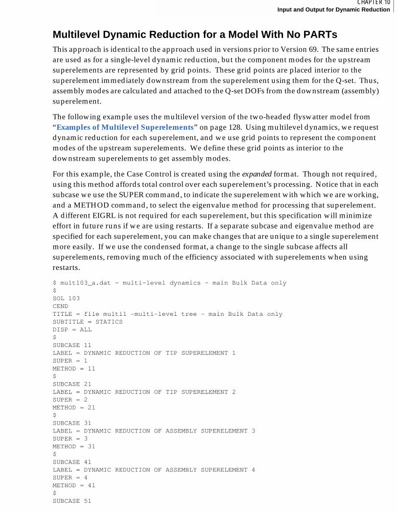
2CHAPTER 10Input and Output for Dynamic Reduction
Multilevel Dynamic Reduction for a Model With No PARTs This approach is identical to the approach used in versions prior to Version 69. The same entries are used as for a single-level dynamic reduction, but the component modes for the upstream superelements are represented by grid points. These grid points are placed interior to the superelement immediately downstream from the superelement using them for the Q-set. Thus, assembly modes are calculated and attached to the Q-set DOFs from the downstream (assembly) superelement.
The following example uses the multilevel version of the two-headed flyswatter model from “Examples of Multilevel Superelements” on page 128. Using multilevel dynamics, we request dynamic reduction for each superelement, and we use grid points to represent the component modes of the upstream superelements. We define these grid points as interior to the downstream superelements to get assembly modes.
For this example, the Case Control is created using the expanded format. Though not required, using this method affords total control over each superelement’s processing. Notice that in each subcase we use the SUPER command, to indicate the superelement with which we are working, and a METHOD command, to select the eigenvalue method for processing that superelement. A different EIGRL is not required for each superelement, but this specification will minimize effort in future runs if we are using restarts. If a separate subcase and eigenvalue method are specified for each superelement, you can make changes that are unique to a single superelement more easily. If we use the condensed format, a change to the single subcase affects all superelements, removing much of the efficiency associated with superelements when using restarts.
$ mult103_a.dat - multi-level dynamics - main Bulk Data only$SOL 103 CENDTITLE = file multi1 -multi-level tree - main Bulk Data onlySUBTITLE = STATICS DISP = ALL$SUBCASE 11LABEL = DYNAMIC REDUCTION OF TIP SUPERELEMENT 1SUPER = 1METHOD = 11$SUBCASE 21LABEL = DYNAMIC REDUCTION OF TIP SUPERELEMENT 2SUPER = 2METHOD = 21$SUBCASE 31LABEL = DYNAMIC REDUCTION OF ASSEMBLY SUPERELEMENT 3SUPER = 3METHOD = 31$SUBCASE 41LABEL = DYNAMIC REDUCTION OF ASSEMBLY SUPERELEMENT 4SUPER = 4METHOD = 41$SUBCASE 51
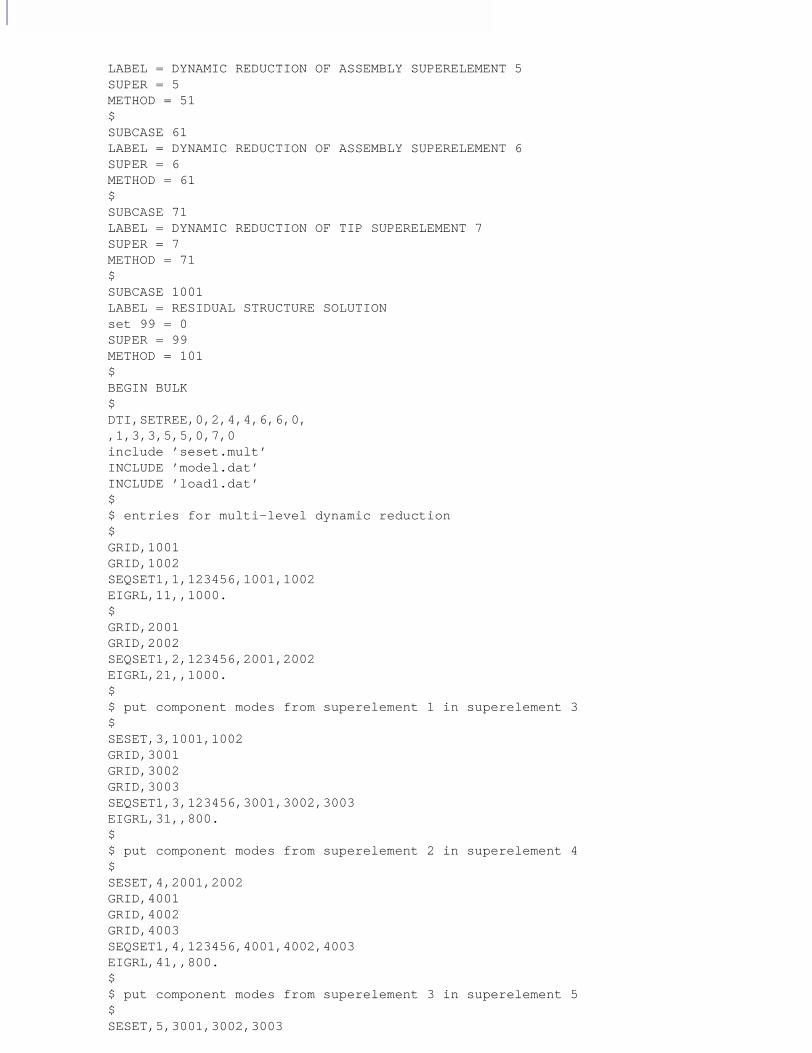
LABEL = DYNAMIC REDUCTION OF ASSEMBLY SUPERELEMENT 5SUPER = 5METHOD = 51$SUBCASE 61LABEL = DYNAMIC REDUCTION OF ASSEMBLY SUPERELEMENT 6SUPER = 6METHOD = 61$SUBCASE 71LABEL = DYNAMIC REDUCTION OF TIP SUPERELEMENT 7SUPER = 7METHOD = 71$SUBCASE 1001LABEL = RESIDUAL STRUCTURE SOLUTIONset 99 = 0SUPER = 99METHOD = 101$BEGIN BULK$DTI,SETREE,0,2,4,4,6,6,0,,1,3,3,5,5,0,7,0include ’seset.mult’INCLUDE ’model.dat’INCLUDE ’load1.dat’$$ entries for multi-level dynamic reduction$GRID,1001GRID,1002SEQSET1,1,123456,1001,1002EIGRL,11,,1000.$GRID,2001GRID,2002SEQSET1,2,123456,2001,2002EIGRL,21,,1000.$$ put component modes from superelement 1 in superelement 3$SESET,3,1001,1002GRID,3001GRID,3002GRID,3003SEQSET1,3,123456,3001,3002,3003EIGRL,31,,800.$$ put component modes from superelement 2 in superelement 4$SESET,4,2001,2002GRID,4001GRID,4002GRID,4003SEQSET1,4,123456,4001,4002,4003EIGRL,41,,800.$$ put component modes from superelement 3 in superelement 5$SESET,5,3001,3002,3003

2CHAPTER 10Input and Output for Dynamic Reduction
GRID,5001GRID,5002GRID,5003SEQSET1,5,123456,5001,THRU,5003EIGRL,51,,600.$$$ put component modes from superelement 4 in superelement 6$SESET,6,4001,4002,4003GRID,6001GRID,6002GRID,6003GRID,6004SEQSET1,6,123456,6001,THRU,6004EIGRL,61,,600.$$ superelement 7$GRID,7001GRID,7002SEQSET1,7,123456,7001,7002EIGRL,71,,1000.$$ ASSEMBLY MODES$EIGRL,101,,400.ENDDATA
To understand how the multilevel process works, we will look at the branch of the tree containing superelements 1, 3, and 5, above the residual structure.
Looking at the Bulk Data, the model definition and the multilevel tree are identical to a static run. The changes for dynamic multilevel processing are shown after the main model definition. By way of explanation, we will look at the input immediately following entries for multilevel dynamic reduction. This area contains the entries used to control the multilevel processing. The entries for superelement 1 are:
GRID,1001GRID,1002SEQSET1,1,123456,1001,1002EIGRL,11,,1000.
We are defining two new grid points that have no connection to the model. (DO NOT CONNECT ANY STRUCTURAL ELEMENTS TO GRID POINTS USED IN A SUPERELEMENT Q-SET.) Both of these points are defined at the Basic Origin (they have no value in the location fields), which would not be allowed if the model had PARTs. However, because (at this point) we are only looking at models without PARTs, this method is acceptable. The SEQSET1 entry instructs MSC.Nastran to use all six DOFs of both of these two new points to represent the modes of superelement 1. Therefore, the first component mode is attached to DOF 1 of GRID 1001, the second mode is attached to DOF 2 of GRID 1001, etc. SUBCASE 11 instructs MSC.Nastran to use EIGRL 11 to solve for modes of superelement 1 up to 1000.0 hz. Because there are no SECSETi entries, the modes are calculated with the exterior points (grid points 35 and 36) held fixed, or the component is cantilevered from the interface with superelement 3.
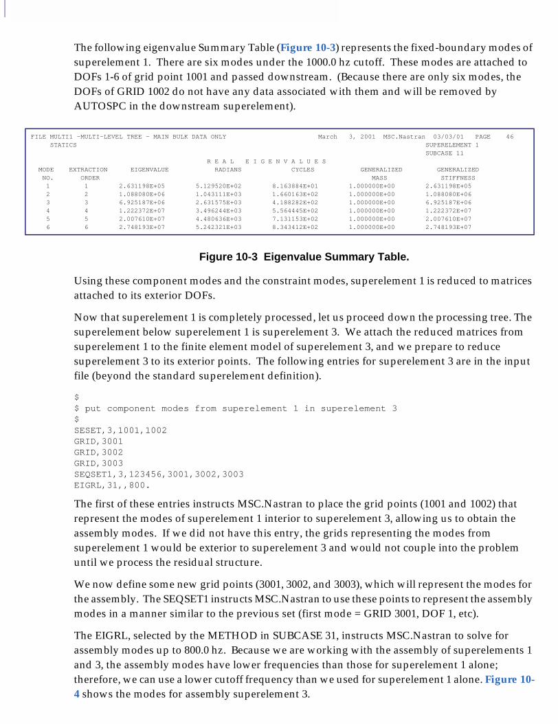
The following eigenvalue Summary Table (Figure 10-3) represents the fixed-boundary modes of superelement 1. There are six modes under the 1000.0 hz cutoff. These modes are attached to DOFs 1-6 of grid point 1001 and passed downstream. (Because there are only six modes, the DOFs of GRID 1002 do not have any data associated with them and will be removed by AUTOSPC in the downstream superelement).
Figure 10-3 Eigenvalue Summary Table.
Using these component modes and the constraint modes, superelement 1 is reduced to matrices attached to its exterior DOFs.
Now that superelement 1 is completely processed, let us proceed down the processing tree. The superelement below superelement 1 is superelement 3. We attach the reduced matrices from superelement 1 to the finite element model of superelement 3, and we prepare to reduce superelement 3 to its exterior points. The following entries for superelement 3 are in the input file (beyond the standard superelement definition).
$$ put component modes from superelement 1 in superelement 3$SESET,3,1001,1002GRID,3001GRID,3002GRID,3003SEQSET1,3,123456,3001,3002,3003EIGRL,31,,800.
The first of these entries instructs MSC.Nastran to place the grid points (1001 and 1002) that represent the modes of superelement 1 interior to superelement 3, allowing us to obtain the assembly modes. If we did not have this entry, the grids representing the modes from superelement 1 would be exterior to superelement 3 and would not couple into the problem until we process the residual structure.
We now define some new grid points (3001, 3002, and 3003), which will represent the modes for the assembly. The SEQSET1 instructs MSC.Nastran to use these points to represent the assembly modes in a manner similar to the previous set (first mode = GRID 3001, DOF 1, etc).
The EIGRL, selected by the METHOD in SUBCASE 31, instructs MSC.Nastran to solve for assembly modes up to 800.0 hz. Because we are working with the assembly of superelements 1 and 3, the assembly modes have lower frequencies than those for superelement 1 alone; therefore, we can use a lower cutoff frequency than we used for superelement 1 alone. Figure 10-4 shows the modes for assembly superelement 3.
FILE MULTI1 -MULTI-LEVEL TREE - MAIN BULK DATA ONLY March 3, 2001 MSC.Nastran 03/03/01 PAGE 46 STATICS SUPERELEMENT 1 SUBCASE 11 R E A L E I G E N V A L U E S MODE EXTRACTION EIGENVALUE RADIANS CYCLES GENERALIZED GENERALIZED NO. ORDER MASS STIFFNESS 1 1 2.631198E+05 5.129520E+02 8.163884E+01 1.000000E+00 2.631198E+05 2 2 1.088080E+06 1.043111E+03 1.660163E+02 1.000000E+00 1.088080E+06 3 3 6.925187E+06 2.631575E+03 4.188282E+02 1.000000E+00 6.925187E+06 4 4 1.222372E+07 3.496244E+03 5.564445E+02 1.000000E+00 1.222372E+07 5 5 2.007610E+07 4.480636E+03 7.131153E+02 1.000000E+00 2.007610E+07 6 6 2.748193E+07 5.242321E+03 8.343412E+02 1.000000E+00 2.748193E+07
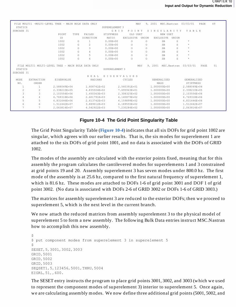
2CHAPTER 10Input and Output for Dynamic Reduction
Figure 10-4 The Grid Point Singularity Table
The Grid Point Singularity Table (Figure 10-4) indicates that all six DOFs for grid point 1002 are singular, which agrees with our earlier results. That is, the six modes for superelement 1 are attached to the six DOFs of grid point 1001, and no data is associated with the DOFs of GRID 1002.
The modes of the assembly are calculated with the exterior points fixed, meaning that for this assembly the program calculates the cantilevered modes for superelements 1 and 3 constrained at grid points 19 and 20. Assembly superelement 3 has seven modes under 800.0 hz. The first mode of the assembly is at 25.6 hz, compared to the first natural frequency of superelement 1, which is 81.6 hz. These modes are attached to DOFs 1-6 of grid point 3001 and DOF 1 of grid point 3002. (No data is associated with DOFs 2-6 of GRID 3002 or DOFs 1-6 of GRID 3003.)
The matrices for assembly superelement 3 are reduced to the exterior DOFs; then we proceed to superelement 5, which is the next level in the current branch.
We now attach the reduced matrices from assembly superelement 3 to the physical model of superelement 5 to form a new assembly. The following Bulk Data entries instruct MSC.Nastran how to accomplish this new assembly.
$$ put component modes from superelement 3 in superelement 5$SESET,5,3001,3002,3003GRID,5001GRID,5002GRID,5003SEQSET1,5,123456,5001,THRU,5004EIGRL,51,,600.
The SESET entry instructs the program to place grid points 3001, 3002, and 3003 (which we used to represent the component modes of superelement 3) interior to superelement 5. Once again, we are calculating assembly modes. We now define three additional grid points (5001, 5002, and
FILE MULTI1 -MULTI-LEVEL TREE - MAIN BULK DATA ONLY MAY 9, 2001 MSC.Nastran 03/03/01 PAGE 49 STATICS SUPERELEMENT 3 SUBCASE 31 G R I D P O I N T S I N G U L A R I T Y T A B L E POINT TYPE FAILED STIFFNESS OLD USET NEW USET ID DIRECTION RATIO EXCLUSIVE UNION EXCLUSIVE UNION 1002 G 1 0.00E+00 O O SB S * 1002 G 2 0.00E+00 O O SB S * 1002 G 3 0.00E+00 O O SB S * 1002 G 4 0.00E+00 O O SB S * 1002 G 5 0.00E+00 O O SB S * 1002 G 6 0.00E+00 O O SB S *
FILE MULTI1 MULTI-LEVEL TREE - MAIN BULK DATA ONLY MAY 9, 2001 MSC.Nastran 03/03/01 PAGE 51 STATICS SUPERELEMENT 3 SUBCASE 31 R E A L E I G E N V A L U E S MODE EXTRACTION EIGENVALUE RADIANS CYCLES GENERALIZED GENERALIZED NO. ORDER MASS STIFFNESS 1 1 2.588049E+04 1.608741E+02 2.560391E+01 1.000000E+00 2.588049E+04 2 2 2.338210E+05 4.835504E+02 7.695943E+01 1.000000E+00 2.338210E+05 3 3 2.103554E+06 1.450363E+03 2.308325E+02 1.000000E+00 2.103554E+06 4 4 6.769318E+06 2.601791E+03 4.140879E+02 1.000000E+00 6.769318E+06 5 5 6.831646E+06 2.613742E+03 4.159899E+02 1.000000E+00 6.831646E+06 6 6 1.512442E+07 3.889012E+03 6.189555E+02 1.000000E+00 1.512442E+07 7 7 2.063814E+07 4.542922E+03 7.230284E+02 1.000000E+00 2.063814E+07
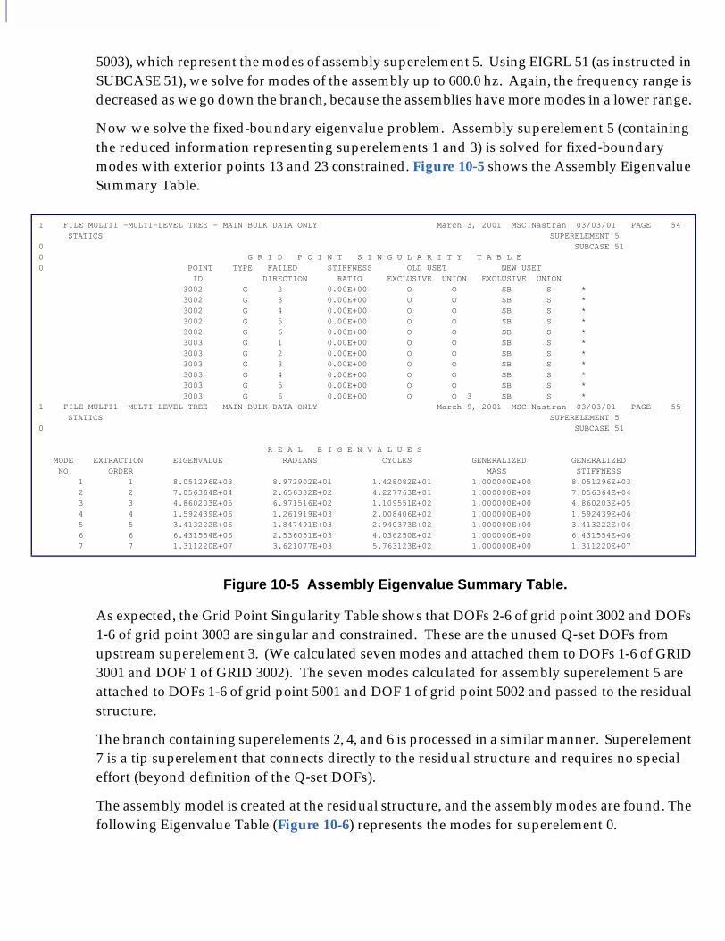
5003), which represent the modes of assembly superelement 5. Using EIGRL 51 (as instructed in SUBCASE 51), we solve for modes of the assembly up to 600.0 hz. Again, the frequency range is decreased as we go down the branch, because the assemblies have more modes in a lower range.
Now we solve the fixed-boundary eigenvalue problem. Assembly superelement 5 (containing the reduced information representing superelements 1 and 3) is solved for fixed-boundary modes with exterior points 13 and 23 constrained. Figure 10-5 shows the Assembly Eigenvalue Summary Table.
Figure 10-5 Assembly Eigenvalue Summary Table.
As expected, the Grid Point Singularity Table shows that DOFs 2-6 of grid point 3002 and DOFs 1-6 of grid point 3003 are singular and constrained. These are the unused Q-set DOFs from upstream superelement 3. (We calculated seven modes and attached them to DOFs 1-6 of GRID 3001 and DOF 1 of GRID 3002). The seven modes calculated for assembly superelement 5 are attached to DOFs 1-6 of grid point 5001 and DOF 1 of grid point 5002 and passed to the residual structure.
The branch containing superelements 2, 4, and 6 is processed in a similar manner. Superelement 7 is a tip superelement that connects directly to the residual structure and requires no special effort (beyond definition of the Q-set DOFs).
The assembly model is created at the residual structure, and the assembly modes are found. The following Eigenvalue Table (Figure 10-6) represents the modes for superelement 0.
1 FILE MULTI1 -MULTI-LEVEL TREE - MAIN BULK DATA ONLY March 3, 2001 MSC.Nastran 03/03/01 PAGE 54 STATICS SUPERELEMENT 5 0 SUBCASE 51 0 G R I D P O I N T S I N G U L A R I T Y T A B L E0 POINT TYPE FAILED STIFFNESS OLD USET NEW USET ID DIRECTION RATIO EXCLUSIVE UNION EXCLUSIVE UNION 3002 G 2 0.00E+00 O O SB S * 3002 G 3 0.00E+00 O O SB S * 3002 G 4 0.00E+00 O O SB S * 3002 G 5 0.00E+00 O O SB S * 3002 G 6 0.00E+00 O O SB S * 3003 G 1 0.00E+00 O O SB S * 3003 G 2 0.00E+00 O O SB S * 3003 G 3 0.00E+00 O O SB S * 3003 G 4 0.00E+00 O O SB S * 3003 G 5 0.00E+00 O O SB S * 3003 G 6 0.00E+00 O O 3 SB S *1 FILE MULTI1 -MULTI-LEVEL TREE - MAIN BULK DATA ONLY March 9, 2001 MSC.Nastran 03/03/01 PAGE 55 STATICS SUPERELEMENT 5 0 SUBCASE 51 R E A L E I G E N V A L U E S MODE EXTRACTION EIGENVALUE RADIANS CYCLES GENERALIZED GENERALIZED NO. ORDER MASS STIFFNESS 1 1 8.051296E+03 8.972902E+01 1.428082E+01 1.000000E+00 8.051296E+03 2 2 7.056364E+04 2.656382E+02 4.227763E+01 1.000000E+00 7.056364E+04 3 3 4.860203E+05 6.971516E+02 1.109551E+02 1.000000E+00 4.860203E+05 4 4 1.592439E+06 1.261919E+03 2.008406E+02 1.000000E+00 1.592439E+06 5 5 3.413222E+06 1.847491E+03 2.940373E+02 1.000000E+00 3.413222E+06 6 6 6.431554E+06 2.536051E+03 4.036250E+02 1.000000E+00 6.431554E+06 7 7 1.311220E+07 3.621077E+03 5.763123E+02 1.000000E+00 1.311220E+07

2CHAPTER 10Input and Output for Dynamic Reduction
Figure 10-6 Eigenvalue Table.
For comparison, we will run the model with no superelements. The following file (modesnose.dat) solves for the modes of the model under 500 hz without any reduction.
$$ file - modesnose.dat - normal modes without superelements $SOL 103 CENDTITLE = file modesnose - normal modes - no superelements DISP = ALL$METHOD = 101$BEGIN BULKINCLUDE ’model.dat’$$ ASSEMBLY MODES$EIGRL,101,,500.ENDDATA
FILE MULTI1 -MULTI-LEVEL TREE - MAIN BULK DATA ONLY MAarch 3, 2001 MSC.Nastran 03/03/01 PAGE 61 STATICS SUPERELEMENT 0 SUBCASE 1001 R E A L E I G E N V A L U E S MODE EXTRACTION EIGENVALUE RADIANS CYCLES GENERALIZED GENERALIZED NO. ORDER MASS STIFFNESS 1 1 1.171680E+03 3.422981E+01 5.447843E+00 1.000000E+00 1.171680E+03 2 2 3.460243E+03 5.882383E+01 9.362103E+00 1.000000E+00 3.460243E+03 3 3 3.992029E+04 1.998006E+02 3.179926E+01 1.000000E+00 3.992029E+04 4 4 6.106046E+04 2.471042E+02 3.932785E+01 1.000000E+00 6.106046E+04 5 5 1.187821E+05 3.446478E+02 5.485241E+01 1.000000E+00 1.187821E+05 6 6 2.309405E+05 4.805627E+02 7.648393E+01 1.000000E+00 2.309405E+05 7 7 2.445625E+05 4.945326E+02 7.870731E+01 1.000000E+00 2.445625E+05 8 8 1.294420E+06 1.137726E+03 1.810747E+02 1.000000E+00 1.294420E+06 9 9 1.471260E+06 1.212955E+03 1.930478E+02 1.000000E+00 1.471260E+06 10 10 2.368725E+06 1.539066E+03 2.449500E+02 1.000000E+00 2.368725E+06 11 11 3.375198E+06 1.837171E+03 2.923949E+02 1.000000E+00 3.375198E+06 12 12 6.109094E+06 2.471658E+03 3.933766E+02 1.000000E+00 6.109094E+06 13 13 6.598576E+06 2.568769E+03 4.088323E+02 1.000000E+00 6.598576E+061 FILE
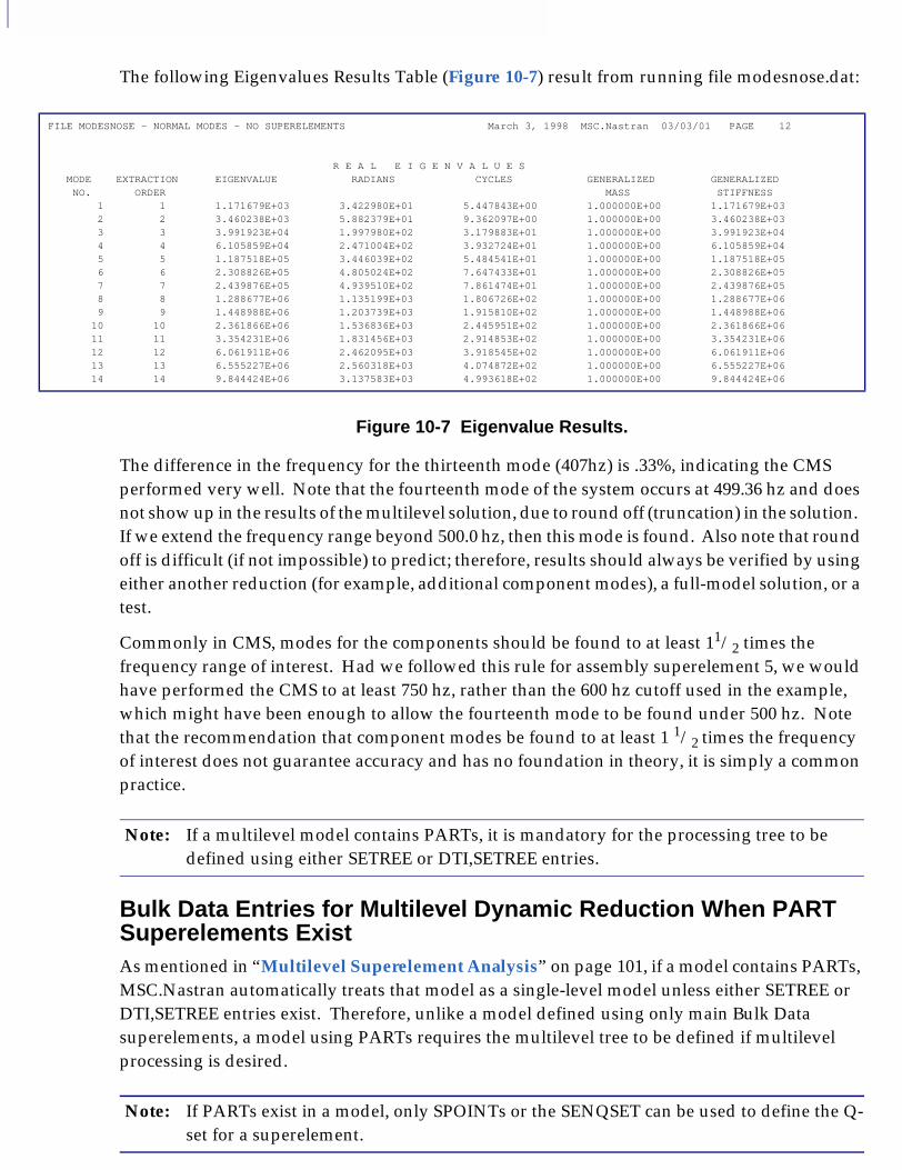
The following Eigenvalues Results Table (Figure 10-7) result from running file modesnose.dat:
Figure 10-7 Eigenvalue Results.
The difference in the frequency for the thirteenth mode (407hz) is .33%, indicating the CMS performed very well. Note that the fourteenth mode of the system occurs at 499.36 hz and does not show up in the results of the multilevel solution, due to round off (truncation) in the solution. If we extend the frequency range beyond 500.0 hz, then this mode is found. Also note that round off is difficult (if not impossible) to predict; therefore, results should always be verified by using either another reduction (for example, additional component modes), a full-model solution, or a test.
Commonly in CMS, modes for the components should be found to at least 11/2 times the frequency range of interest. Had we followed this rule for assembly superelement 5, we would have performed the CMS to at least 750 hz, rather than the 600 hz cutoff used in the example, which might have been enough to allow the fourteenth mode to be found under 500 hz. Note that the recommendation that component modes be found to at least 1 1/2 times the frequency of interest does not guarantee accuracy and has no foundation in theory, it is simply a common practice.
Bulk Data Entries for Multilevel Dynamic Reduction When PART Superelements ExistAs mentioned in “Multilevel Superelement Analysis” on page 101, if a model contains PARTs, MSC.Nastran automatically treats that model as a single-level model unless either SETREE or DTI,SETREE entries exist. Therefore, unlike a model defined using only main Bulk Data superelements, a model using PARTs requires the multilevel tree to be defined if multilevel processing is desired.
FILE MODESNOSE - NORMAL MODES - NO SUPERELEMENTS March 3, 1998 MSC.Nastran 03/03/01 PAGE 12 R E A L E I G E N V A L U E S MODE EXTRACTION EIGENVALUE RADIANS CYCLES GENERALIZED GENERALIZED NO. ORDER MASS STIFFNESS 1 1 1.171679E+03 3.422980E+01 5.447843E+00 1.000000E+00 1.171679E+03 2 2 3.460238E+03 5.882379E+01 9.362097E+00 1.000000E+00 3.460238E+03 3 3 3.991923E+04 1.997980E+02 3.179883E+01 1.000000E+00 3.991923E+04 4 4 6.105859E+04 2.471004E+02 3.932724E+01 1.000000E+00 6.105859E+04 5 5 1.187518E+05 3.446039E+02 5.484541E+01 1.000000E+00 1.187518E+05 6 6 2.308826E+05 4.805024E+02 7.647433E+01 1.000000E+00 2.308826E+05 7 7 2.439876E+05 4.939510E+02 7.861474E+01 1.000000E+00 2.439876E+05 8 8 1.288677E+06 1.135199E+03 1.806726E+02 1.000000E+00 1.288677E+06 9 9 1.448988E+06 1.203739E+03 1.915810E+02 1.000000E+00 1.448988E+06 10 10 2.361866E+06 1.536836E+03 2.445951E+02 1.000000E+00 2.361866E+06 11 11 3.354231E+06 1.831456E+03 2.914853E+02 1.000000E+00 3.354231E+06 12 12 6.061911E+06 2.462095E+03 3.918545E+02 1.000000E+00 6.061911E+06 13 13 6.555227E+06 2.560318E+03 4.074872E+02 1.000000E+00 6.555227E+06 14 14 9.844424E+06 3.137583E+03 4.993618E+02 1.000000E+00 9.844424E+06
Note: If a multilevel model contains PARTs, it is mandatory for the processing tree to be defined using either SETREE or DTI,SETREE entries.
Note: If PARTs exist in a model, only SPOINTs or the SENQSET can be used to define the Q-set for a superelement.

2CHAPTER 10Input and Output for Dynamic Reduction
When PARTs exist, only SPOINTs or the SENQSET can be used to define the Q-set DOFs of a superelement. Unless you manually request the program to couple these modes into the downstream superelement, the modes are passed directly to the residual structure and will not be coupled into any downstream superelement component modes. Although not identical, this method is similar to the Benfield-Hruda method of CMS.
In my opinion, using this default (passing modes directly to the residual and not including these modes in assembly component modes) is not as accurate as coupling a superelement’s modes into the downstream superelement (including the effect of the superelement’s modes on the assembly modes). Example problems can be created for any of the modern techniques, wherein one approach greatly outperforms all other approaches. However, (once again, my opinion) coupling upstream superelements into assembly modes generally provides a greater degree of accuracy for a smaller number of DOFs at the final (residual structure) solution.
To prevent the program from automatically passing a superelement’s modes all the way to the residual structure solution, you must manually put the DOFs representing those modes into the downstream superelement that you want to include these modes. Therefore, you must define additional SPOINTs, which are placed interior to the downstream superelement, and use the SECONCT entry to instruct the program to attach the upstream modes to these DOFs. Once the model contains a PART, you must repeat this process for both main Bulk Data superelements and PARTs if you wish to get assembly modes.
Note that any Q-set DOFs defined using the SENQSET entry automatically belong to the residual structure. These DOFs cannot be combined into downstream superelement assemblies until the final (residual structure) solution.
The following input demonstrates how to couple the modes from an upstream superelement into a downstream superelement. We assume that superelement 1 is above superelement 3 in our superelement tree. We will perform CMS on superelement 1, but now we want to obtain assembly modes when processing superelement 3; that is, we want to observe the behavior of the assembly of superelements 1 and 3. The following input accomplishes this task.
SOL 103CENDTITLE = ASSEMBLY MODESDISP(PLOT)=ALL$SUBCASE 1LABEL = CMS OF SUPERELEMENT 1SUPER = 1METHOD = 100$SUBCASE 2LABEL = ASSEMBLY MODES OF SE 1 AND 3SUPER = 3METHOD = 101...BEGIN BULK$$ MAIN BULK DATA SECTION $$ ENTRIES TO “COUPLE” MODES FROM SUPERELEMENT 1 INTO ASSEMBLY SE 3$
SETREE,3,1 $ place SE 1 above SE 3 in tree$$ “CONNECT” UPSTREAM MODES TO DOF INTERIOR TO SE 3$SECONCT,1,3 ,1001,11001,1002,11002,1003,11003,1004,11004 ,1005,11005,1006,11006,1007,11007,1008,11008 ,1009,11009,1010,11010,1011,11011,1012,11012$..BEGIN SUPER=1$$ DEFINE Q-SET FOR SE 1$SPOINT,1001,THRU,1012QSET1,0,1001,THRU,1012EIGRL,100,......BEGIN SUPER=3$$ DEFINE DOF TO ATTACH UPSTREAM MODES TO$SPOINT,11001,THRU,11012$$ DEFINE Q-SET FOR “ASSEMBLY” SE 3$SPOINT,3001,THRU,3015QSET1,0,3001,THRU,3015EIGRL,101,......ENDDATA
The Case Control in the above input should be self-explanatory: We are requesting CMS for superelements 1 and 3. In the Partitioned Bulk Data Section for superelement 1, we define SPOINTs 1001 through 1012. These SPOINTs are used as the DOFs to represent the component modes calculated using EIGRL number 100 (also in this section). Once superelement 1 is processed we are ready to continue down the branch and begin processing superelement 3, which is our assembly. In the partitioned Bulk Data for superelement 3 we not only define SPOINTs 3001 through 3015, which will represent the assembly modes, but we also define SPOINTs 11001 through 11012, to which the modes from superelement 1 are connected.
Sample of Multilevel CMS Using PARTsThe following input file is similar to mult103-a.dat (shown earlier in this section), except that PARTs are used to define the superelements.
Note: Because each Partitioned Bulk Data Section is treated separately, the same numbers can be used for the SPOINTS as are used in the upstream superelement, which still requires the use of a SECONCT entry to attach the modes.) The upstream modes are attached to these DOFs by the use of the SECONCT entry in the Main Bulk Data Section. This entry instructs the program to connect the DOFs that represent the modes of superelement 1 to the new DOFs we have defined interior to superelement 3.

2CHAPTER 10Input and Output for Dynamic Reduction
$ use spoints$ se1m103p - multi-level using PARTsID SE, SAMPLE PROBLEM - MULTI-LEVEL DYNAMICSSOL 103CEND$TITLE = file -multi-level tree - PARTsSUBTITLE = MODES DISP = ALL$SUBCASE 11LABEL = DYNAMIC REDUCTION OF TIP SUPERELEMENT 1SUPER = 1METHOD = 11$SUBCASE 21LABEL = DYNAMIC REDUCTION OF TIP SUPERELEMENT 2SUPER = 2METHOD = 21$SUBCASE 31LABEL = DYNAMIC REDUCTION OF ASSEMBLY SUPERELEMENT 3SUPER = 3METHOD = 31$SUBCASE 41LABEL = DYNAMIC REDUCTION OF ASSEMBLY SUPERELEMENT 4SUPER = 4METHOD = 41$SUBCASE 51LABEL = DYNAMIC REDUCTION OF ASSEMBLY SUPERELEMENT 5SUPER = 5METHOD = 51$SUBCASE 61LABEL = DYNAMIC REDUCTION OF ASSEMBLY SUPERELEMENT 6SUPER = 6METHOD = 61$SUBCASE 71LABEL = DYNAMIC REDUCTION OF TIP SUPERELEMENT 7SUPER = 7METHOD = 71$SUBCASE 1001LABEL = RESIDUAL STRUCTURE SOLUTIONset 99 = 0SUPER = 99METHOD = 101$include ’plot.blk’$BEGIN BULK$setree,3,1setree,5,3setree,4,2setree,6,4setree,0,5,6,7EIGRL,101,,500.
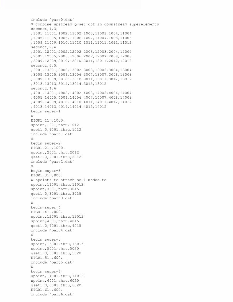
include ’part0.dat’$ combine upstream Q-set dof in downstream superelementsseconct,1,3,,1001,11001,1002,11002,1003,11003,1004,11004,1005,11005,1006,11006,1007,11007,1008,11008,1009,11009,1010,11010,1011,11011,1012,11012seconct,2,4,2001,12001,2002,12002,2003,12003,2004,12004,2005,12005,2006,12006,2007,12007,2008,12008,2009,12009,2010,12010,2011,12011,2012,12012seconct,3,5,,3001,13001,3002,13002,3003,13003,3004,13004,3005,13005,3006,13006,3007,13007,3008,13008,3009,13009,3010,13010,3011,13011,3012,13012,3013,13013,3014,13014,3015,13015seconct,4,6,4001,14001,4002,14002,4003,14003,4004,14004,4005,14005,4006,14006,4007,14007,4008,14008,4009,14009,4010,14010,4011,14011,4012,14012,4013,14013,4014,14014,4015,14015begin super=1$EIGRL,11,,1000.spoint,1001,thru,1012qset1,0,1001,thru,1012include ’part1.dat’$begin super=2EIGRL,21,,1000.spoint,2001,thru,2012qset1,0,2001,thru,2012include ’part2.dat’$begin super=3EIGRL,31,,800.$ spoints to attach se 1 modes tospoint,11001,thru,11012spoint,3001,thru,3015qset1,0,3001,thru,3015include ’part3.dat’$begin super=4EIGRL,41,,800.spoint,12001,thru,12012spoint,4001,thru,4015qset1,0,4001,thru,4015include ’part4.dat’$begin super=5spoint,13001,thru,13015spoint,5001,thru,5020qset1,0,5001,thru,5020EIGRL,51,,600.include ’part5.dat’$begin super=6spoint,14001,thru,14015spoint,6001,thru,6020qset1,0,6001,thru,6020EIGRL,61,,600.include ’part6.dat’

2CHAPTER 10Input and Output for Dynamic Reduction
$begin super=7EIGRL,71,,1000.spoint,7001,thru,7010qset1,0,7001,thru,7010include ’part7.dat’
$ENDDATA
The Executive and Case Control Sections of this file are identical to mult103_a.dat. The Bulk Data is for the same model, except that PARTs are used to define the model. The tree is identical to mult103_a.dat, and the answers are the same.
Notice that (as shown earlier) SECONCT entries are used in the Main Bulk Data Section to place the modes from upstream superelements into the downstream superelements. The use of SECONCT entries is comparable to employing grid entries and SESET entries when the model uses main Bulk Data superelements only.
The procedure shown in this sample applies to all multilevel models using PARTs, regardless of whether main Bulk Data superelements are defined. If a PART is defined, then this procedure must be used to couple the modes into downstream superelements, unless you wish all upstream superelement modes to be passed directly to the residual structure.

MSC.Nastran Superelements User’s Guide
CHAPTER
11 Dynamic Loading on Superelements
■ How to Define Dynamic Loadings on Superelements
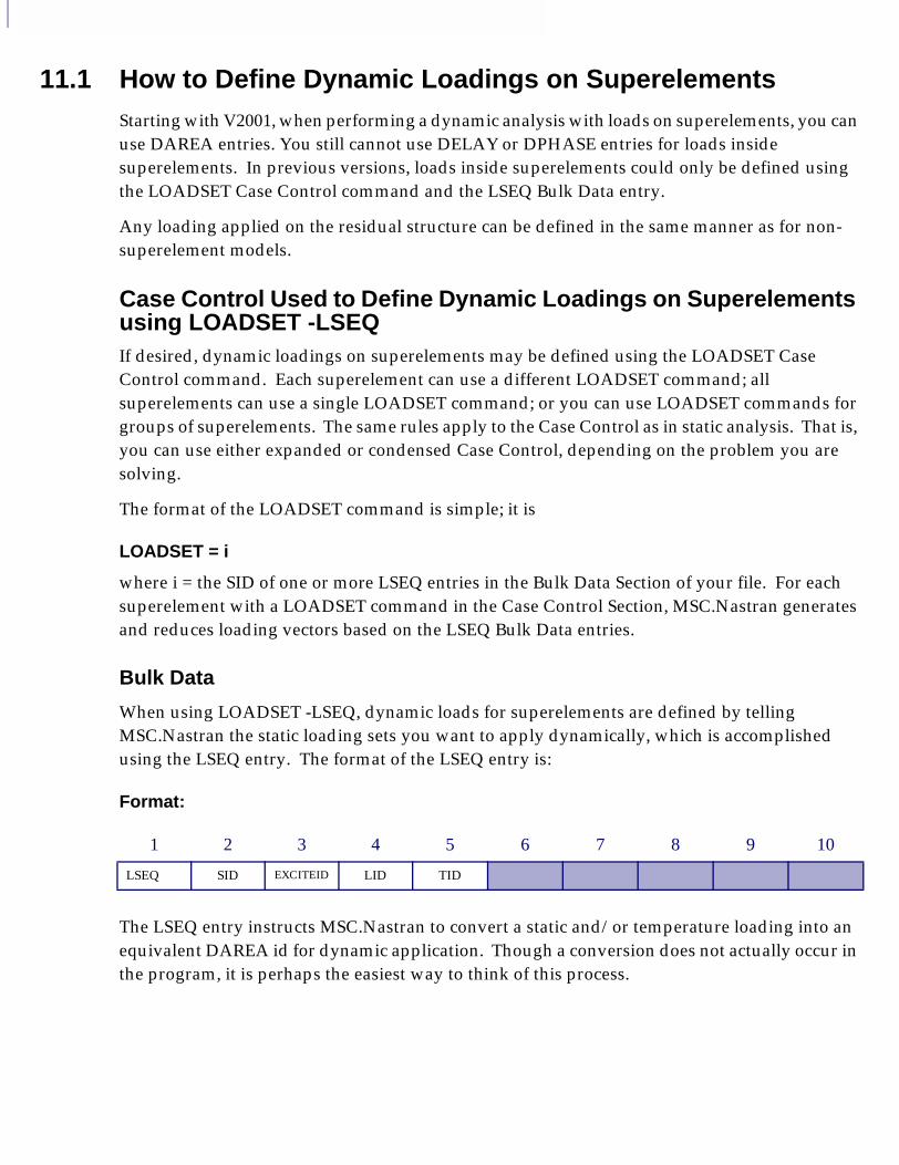
11.1 How to Define Dynamic Loadings on SuperelementsStarting with V2001, when performing a dynamic analysis with loads on superelements, you can use DAREA entries. You still cannot use DELAY or DPHASE entries for loads inside superelements. In previous versions, loads inside superelements could only be defined using the LOADSET Case Control command and the LSEQ Bulk Data entry.
Any loading applied on the residual structure can be defined in the same manner as for non-superelement models.
Case Control Used to Define Dynamic Loadings on Superelements using LOADSET -LSEQIf desired, dynamic loadings on superelements may be defined using the LOADSET Case Control command. Each superelement can use a different LOADSET command; all superelements can use a single LOADSET command; or you can use LOADSET commands for groups of superelements. The same rules apply to the Case Control as in static analysis. That is, you can use either expanded or condensed Case Control, depending on the problem you are solving.
The format of the LOADSET command is simple; it is
LOADSET = i
where i = the SID of one or more LSEQ entries in the Bulk Data Section of your file. For each superelement with a LOADSET command in the Case Control Section, MSC.Nastran generates and reduces loading vectors based on the LSEQ Bulk Data entries.
Bulk Data
When using LOADSET -LSEQ, dynamic loads for superelements are defined by telling MSC.Nastran the static loading sets you want to apply dynamically, which is accomplished using the LSEQ entry. The format of the LSEQ entry is:
Format:
The LSEQ entry instructs MSC.Nastran to convert a static and/or temperature loading into an equivalent DAREA id for dynamic application. Though a conversion does not actually occur in the program, it is perhaps the easiest way to think of this process.
1 2 3 4 5 6 7 8 9 10
LSEQ SID EXCITEID LID TID
2CHAPTER 11Dynamic Loading on Superelements
The fields on this entry are used as follows:
Once again, it is easiest to think of this entry as instructing the program to internally convert a static loading into DAREA entries. What really happens when the LOADSET-LSEQ combination is used is described below.
When a LOADSET Case Control command is encountered while processing a superelement, the program finds all LSEQ entries that match the SID on the LOADSET command. Using these LSEQ entries, a column in the static loading matrix (PJ) is created for the current superelement for each EXCITEID set identified on these entries. The program then places the associated loading (LID and/or TID) data into that column of the loading matrix and processes that matrix for the superelement. The OLOAD RESULTANT output for the superelement is defined for the loadings using this manner, and each column corresponds with a EXCITEID set defined on the LSEQ entries, in ascending order. These loading matrices go through the SELG and SELR operations for all superelements in the model. At the residual structure the reduced superelement loading matrices are combined with loadings defined for the residual structure to form a PG matrix that is associated with the EXCITEID sets selected. These loadings are then combined with DAREA entries (only allowed for the residual structure) to define the complete set of dynamic loadings to be applied (selected by TLOADi or RLOADi entries).
Once again, DAREA, DELAY and DPHASE entries can be used only for the residual structure. If you want to apply a delay or phase angle to a loading on a superelement, you must do so in the actual dynamic loading definition using the RLOADi or TLOADi and its associated data.
Example Demonstrating Dynamic Loads on SuperelementsUsing the model (cantbeam.dat) from “Introduction to Superelements in Dynamic Analysis” in Chapter 9, we will look at defining dynamic loadings on superelements. For this example let us assume that we have a loading of two units applied in the Y-direction at grid point 11 of the model. This loading is applied dynamically in a transient solution and oscillates at 10 hz in a sine function.
SID set id for this LSEQ. Any number of LSEQ entries can use the same SID selected by the LOADSET command.
EXCITEID set id of the DAREA set this entry is defining. This is the id used on the TLOADi or RLOADi entries to apply this loading dynamically. All loads with the same DAREA id are combined at the residual structure.
LID set id of the static loading to be converted into DAREA.
TID set id of the temperature loading to be converted into DAREA.
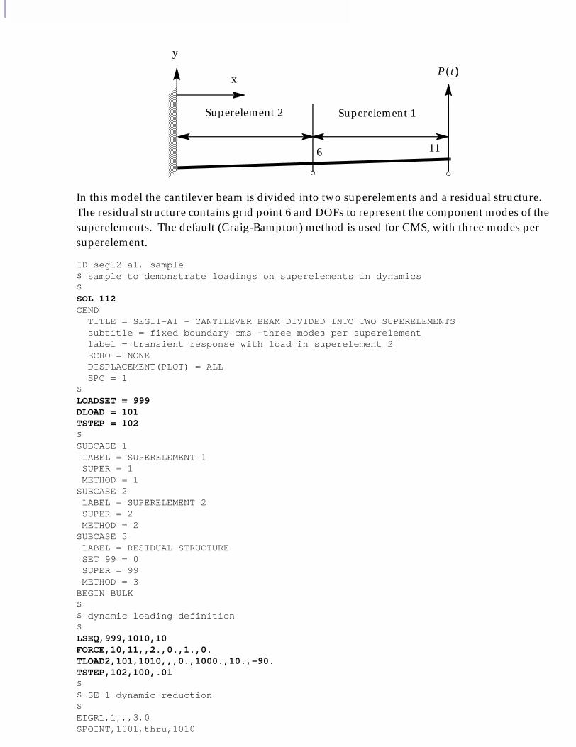
In this model the cantilever beam is divided into two superelements and a residual structure. The residual structure contains grid point 6 and DOFs to represent the component modes of the superelements. The default (Craig-Bampton) method is used for CMS, with three modes per superelement.
ID seg12-a1, sample$ sample to demonstrate loadings on superelements in dynamics$ SOL 112CEND TITLE = SEG11-A1 - CANTILEVER BEAM DIVIDED INTO TWO SUPERELEMENTS subtitle = fixed boundary cms -three modes per superelement label = transient response with load in superelement 2 ECHO = NONE DISPLACEMENT(PLOT) = ALL SPC = 1$LOADSET = 999DLOAD = 101TSTEP = 102$SUBCASE 1 LABEL = SUPERELEMENT 1 SUPER = 1 METHOD = 1SUBCASE 2 LABEL = SUPERELEMENT 2 SUPER = 2 METHOD = 2SUBCASE 3 LABEL = RESIDUAL STRUCTURE SET 99 = 0 SUPER = 99 METHOD = 3BEGIN BULK$$ dynamic loading definition$LSEQ,999,1010,10FORCE,10,11,,2.,0.,1.,0.TLOAD2,101,1010,,,0.,1000.,10.,-90.TSTEP,102,100,.01$$ SE 1 dynamic reduction$EIGRL,1,,,3,0SPOINT,1001,thru,1010
y
x
Superelement 2 Superelement 1
P t( )
116

2CHAPTER 11Dynamic Loading on Superelements
SEQSET1,1,0,1001,thru,1010$$ se 2 dynamic reduction$EIGRL,2,,,3,0spoint,2001,thru,2010seqset1,2,0,2001,thru,2010$$ residual structure$EIGRL,3,,,10,0$include ’cantbeam.dat’ENDDATA
The above file uses SOL 112 (modal transient) to perform the solution. SOL 109 (direct transient) could have also been used. The solution selected is independent of the methodology used to reduce the superelements. The entries that are used to define the dynamic loading are highlighted in bold. Though not required, the LOADSET, DLOAD, and TSTEP commands are above the first SUBCASE in the Case Control. These commands can occur within the SUBCASEs; however, the first approach is easier. The DLOAD and TSTEP commands are mandatory for the residual structure SUBCASE and optional for the superelements SUBCASEs. If you are not requesting OLOAD output, you do not need to place these commands in the superelement SUBCASEs. (The only purpose these commands serve for superelements is to request OLOAD output.) MSC.Nastran generates static loading vectors at the superelement level. The program then passes these vectors through the reduction process until the residual structure where these static vectors are combined with associated DAREA entries, and the information from the DLOAD and TSTEP is used to solve the problem.
You can use a different LOADSET command for each superelement in the model, but it is easier to use a single LOADSET command and to place this command above all SUBCASEs. In this model the LOADSET command instructs MSC.Nastran to use LSEQ set 999 to create static loading vectors that will be applied dynamically.
In the Bulk Data Section, the LSEQ, TLOAD, and TSTEP entries define the dynamic solution. The LSEQ entry (set 999) instructs the program to create a static loading vector based on static load set 10. This loading vector is associated with EXCITEID set 1010.
Static loading 10 is defined by the FORCE entry, which states that we have a 2.0 unit force in the positive Y-direction on grid point 11. This grid point is interior to superelement 1; therefore, when superelement 1 is processed, a loading vector is generated. During the processing, the output for superelement 1 includes OLOAD RESULTANT, as follows:
FIXED BOUNDARY CMS -THREE MODES PER SUPERELEMENT SUPERELEMENT 1 0 TRANSIENT RESPONSE WITH LOAD IN SUPERELEMENT 2 0 RESULTANTS ABOUT ORIGIN OF SUPERELEMENT BASIC COORDINATE SYSTEM IN SUPERELEMENT BASIC SYSTEM COORDINATES.0 OLOAD RESULTANT 0 T1 T2 T3 R1 R2 R30 1 0.0000000E+00 2.0000000E+00 0.0000000E+00 0.0000000E+00 0.0000000E+00 2.0000000E+01
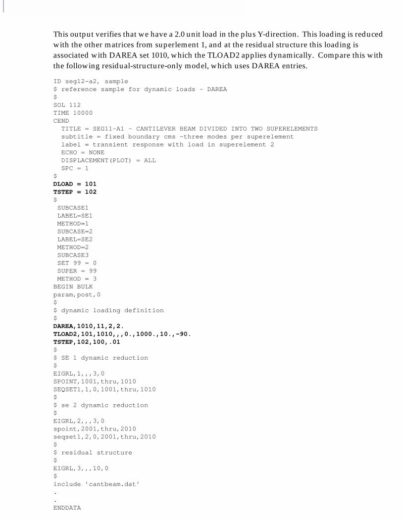
This output verifies that we have a 2.0 unit load in the plus Y-direction. This loading is reduced with the other matrices from superlement 1, and at the residual structure this loading is associated with DAREA set 1010, which the TLOAD2 applies dynamically. Compare this with the following residual-structure-only model, which uses DAREA entries.
ID seg12-a2, sample$ reference sample for dynamic loads - DAREA$ SOL 112TIME 10000CEND TITLE = SEG11-A1 - CANTILEVER BEAM DIVIDED INTO TWO SUPERELEMENTS subtitle = fixed boundary cms -three modes per superelement label = transient response with load in superelement 2 ECHO = NONE DISPLACEMENT(PLOT) = ALL SPC = 1$DLOAD = 101TSTEP = 102$ SUBCASE1 LABEL=SE1 METHOD=1 SUBCASE=2 LABEL=SE2 METHOD=2 SUBCASE3 SET 99 = 0 SUPER = 99 METHOD = 3BEGIN BULKparam,post,0 $$ dynamic loading definition$DAREA,1010,11,2,2.TLOAD2,101,1010,,,0.,1000.,10.,-90.TSTEP,102,100,.01$$ SE 1 dynamic reduction$EIGRL,1,,,3,0SPOINT,1001,thru,1010SEQSET1,1,0,1001,thru,1010$$ se 2 dynamic reduction$EIGRL,2,,,3,0spoint,2001,thru,2010seqset1,2,0,2001,thru,2010$$ residual structure$EIGRL,3,,,10,0$include ’cantbeam.dat’..ENDDATA
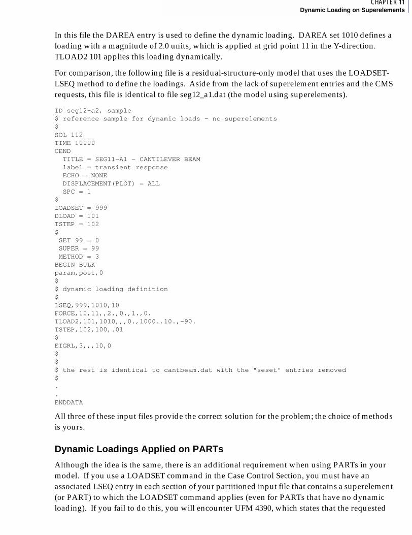
2CHAPTER 11Dynamic Loading on Superelements
In this file the DAREA entry is used to define the dynamic loading. DAREA set 1010 defines a loading with a magnitude of 2.0 units, which is applied at grid point 11 in the Y-direction. TLOAD2 101 applies this loading dynamically.
For comparison, the following file is a residual-structure-only model that uses the LOADSET-LSEQ method to define the loadings. Aside from the lack of superelement entries and the CMS requests, this file is identical to file seg12_a1.dat (the model using superelements).
ID seg12-a2, sample$ reference sample for dynamic loads - no superelements$ SOL 112TIME 10000CEND TITLE = SEG11-A1 - CANTILEVER BEAM label = transient response ECHO = NONE DISPLACEMENT(PLOT) = ALL SPC = 1$LOADSET = 999DLOAD = 101TSTEP = 102$ SET 99 = 0 SUPER = 99 METHOD = 3BEGIN BULKparam,post,0 $$ dynamic loading definition$LSEQ,999,1010,10FORCE,10,11,,2.,0.,1.,0.TLOAD2,101,1010,,,0.,1000.,10.,-90.TSTEP,102,100,.01$EIGRL,3,,,10,0$$$ the rest is identical to cantbeam.dat with the "seset" entries removed$..ENDDATA
All three of these input files provide the correct solution for the problem; the choice of methods is yours.
Dynamic Loadings Applied on PARTs
Although the idea is the same, there is an additional requirement when using PARTs in your model. If you use a LOADSET command in the Case Control Section, you must have an associated LSEQ entry in each section of your partitioned input file that contains a superelement (or PART) to which the LOADSET command applies (even for PARTs that have no dynamic loading). If you fail to do this, you will encounter UFM 4390, which states that the requested
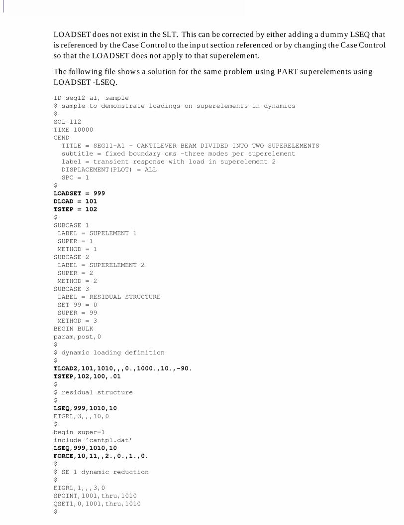
LOADSET does not exist in the SLT. This can be corrected by either adding a dummy LSEQ that is referenced by the Case Control to the input section referenced or by changing the Case Control so that the LOADSET does not apply to that superelement.
The following file shows a solution for the same problem using PART superelements using LOADSET -LSEQ.
ID seg12-a1, sample$ sample to demonstrate loadings on superelements in dynamics$ SOL 112TIME 10000CEND TITLE = SEG11-A1 - CANTILEVER BEAM DIVIDED INTO TWO SUPERELEMENTS subtitle = fixed boundary cms -three modes per superelement label = transient response with load in superelement 2 DISPLACEMENT(PLOT) = ALL SPC = 1$LOADSET = 999DLOAD = 101TSTEP = 102$SUBCASE 1 LABEL = SUPELEMENT 1 SUPER = 1 METHOD = 1SUBCASE 2 LABEL = SUPERELEMENT 2 SUPER = 2 METHOD = 2SUBCASE 3 LABEL = RESIDUAL STRUCTURE SET 99 = 0 SUPER = 99 METHOD = 3BEGIN BULKparam,post,0 $$ dynamic loading definition$TLOAD2,101,1010,,,0.,1000.,10.,-90.TSTEP,102,100,.01$$ residual structure$LSEQ,999,1010,10EIGRL,3,,,10,0$begin super=1include ’cantp1.dat’LSEQ,999,1010,10FORCE,10,11,,2.,0.,1.,0.$$ SE 1 dynamic reduction$EIGRL,1,,,3,0SPOINT,1001,thru,1010QSET1,0,1001,thru,1010$

2CHAPTER 11Dynamic Loading on Superelements
begin super=2include ’cantp2.dat’$$ se 2 dynamic reduction$LSEQ,999,1010,10EIGRL,2,,,3,0spoint,2001,thru,2010qset1,0,2001,thru,2010ENDDATA
This file is similar to seg12_a1.dat, except that PARTs are used. The loading-related input is highlighted in bold. The Case Control is identical to seg12_a1.dat. The only differences occur in the Bulk Data Section. In the Main Bulk Data Section and in the section for PART 2, there is an LSEQ entry (a copy of the one used in PART 1), which has no associated static loading entries. This is to avoid UFM 4390. In the section for PART 1, we have the LSEQ and the associated loading entry for grid point 11. Remember that PARTs need to be self-contained, so if OLOAD (applied loading) output is desired for PART 1, you must also copy the TLOAD2 and TSTEP entries into its data section. Although these entries are not used as part of the solution, the data recovery operation uses them to generate a time history of the applied loading (if requested).


MSC.Nastran Superelement User’s Guide
APPENDIX
A References
■ References

A.1 References1. Craig, R.R. and Bampton, M.C.C. “Coupling of Substructures for Dynamic Analysis,”
AIAA Journal, Vol. 6, No. 7, July 1968.
2. Craig, R.R. Structural Dynamics: An Introduction to Computer Methods, John Wiley and Sons, New York, 1981.
3. Gockel, M.A. MSC.Nastran Handbook for Superelement Analysis
4. The MSC.Nastran Reference Manual, Version 68

2CHAPTER
Aadvantages of using superelements 3assembly superelement 106attachment degrees-of-freedom (DOFs) 7Automatically Connecting PARTs to Other Components of the Model 35AUTOSPC 66Bbasic coordinate system 41
PARTs 41BC 177Benfield-Hruda 209boundary element 48, 51boundary points 35branch elements 48, 51B-set 160Bulk Data
partitioning 47, 49constraints 65
Bulk Data entriesASET 40ASET1 40BEGIN SUPER 25BSET 40, 189BSET1 189CSET 40, 189CSET1 40, 189CSUPEXT 48, 68DAREA 216, 217DELAY 216, 217DEPHASE 216DPHASE 217DTI,SETREE 102, 119, 120DYNRED 176EIGR 161, 176EIGRL 161, 176EPOINT 48GRAV 44GRID 46, 180LSEQ 216, 221PLOTEL 68POINT 43QSET 189QSET1 189RFORCE 44RLOADi 217SEBNDRY 36
as used in automatic connection logic 36SEBSET 179SEBSET1 179SEBULK 36
as used in connection logic 37SECONCT 36, 190

as used in automatic connection logic 38SECSET 179SECSET1 165, 179SEELT 48SEEXCLD 36
as used in automatic connection logic 39SELOC
used to move and/or rotate PARTs 40SENQSET 180, 189SEQSET 179SEQSET1 150, 179SESET 46SESUP 160, 161, 180SETREE 102, 120single-level dynamic reduction of PARTs 188SPOINT 48, 180, 189SUPORT 160, 189TLOADi 217
CCase Control
condensed 71, 73default values - setting 71expanded 70, 72manual processing commands 69multiple loading conditions 75parameters 80partitioning 69, 70, 97
example 97Case Control commands
DYNRED 176LOADSET 216, 217, 221METHOD 176MPC 70SEALL 69SEDR 69SEEX 69SEEXclude 69SEFINAL 69, 120SEKR 69SELG 69, 217SELR 69, 217SEMG 69SEMR 69SPC 70SUPER 69, 97
partitioning 97Case Control in Superelement Analysis 69CASES 70CASES table 97CMS 150CMS with Exterior DOF in the C- and/or R-SET 160collector superelement 102, 107

2CHAPTER
component modal synthesis 2, 145, 176component modes 150concentrated masses 49connecting PARTs 35constraints
single-point 65Constraints on Boundary Points 35Controlling the Connection Between PARTs and the Rest of the Model 36cookie-cutter 24coordinate system
main bulk data basic 41Craig-Bampton CMS 148, 174, 218C-set 160Ddata recovery 18datablock
CASES 97Defining Superelements in the Main Bulk Data Section 46disjoint superelements 104DMIG,UACCEL 86DTI,SETREE 200Dynamic Loading Output 219Dynamic Loadings Applied on PARTs 221dynamic reduction 144
Bulk Data entries for Main Bulk Data Superelements 179, 200, 208Case Control 176procedures 142samples 181
dynamic transformation 149dynamic transformation matrix 142, 144DYNRED
generalized dynamic reduction 161EEPSRC 162example
single-level analysis 58exterior degrees-of-freedom 7exterior grid points 50exterior points
manually defining for PARTs 40external degrees-of-freedom (DOFs) 7external superelements 5FFIXEDB 161fixed-boundary component modal synthesis sample 150fixed-boundary displacements 8fixed-boundary dynamic reduction 148fixed-boundary modes 149fixed-boundary solution 18, 19Flow Chart for Superelement Processing 12free-free dynamic reduction 159F-set 160

fundamentals of superelement analysis 5Ggeneralized dynamic reduction 145, 161, 176generalized mass and stiffness 149GPSP 66GRDPNT 86
parameters 81Grid Point Singularity Processor 66Guyan Reduction 144HHow to Define Dynamic Loadings on Superelements 216Iimage superelement 5individual superelement case control 70Individual Superelement Map 138inertia relief 84, 85
PARAM,INREL 86SUPORT 86
inertia relief modes 162input
partitioning 7simplified for single-level analysis 57
INREL DMAP Module 161INRLM 162interior degrees-of-freedom (DOFs) 7interior grid points 50interior vs exterior 47KK6ROT 80KGG 151KJJ 123, 151Llarge problem capabilites 3load sequence number 70, 72load1.dat 75loading sequence 73loadings
rotated 44loadprt1.dat 29loadprt2.dat 33Loads in Static Analysis 63LOADSET
UFM 4390 221, 223MMain Bulk Data Section 25, 46main bulk data superelements 24, 25manually defining exterior points 40MATREDU 164MB 44mechanism 84MGG 151mixed-boundary dynamic reduction 160

2CHAPTER
MJJ 151, 155modal transient 219model.dat 21Moving and/or Rotating PARTs 40Multilevel Analysis 106multilevel dynamic reduction 200multilevel superelement analysis 102multilevel tree 50multiple constraint conditions 70multiple loading conditions 75Multipoint Constraints (MPCs) 66OOLOAD output for superelements 219OLOAD RESULTANT 91, 219
in dynamic analysis 217One Loading Condition-Expanded Case Control 72output
SEMAP 52Superelement MAP 52
output coordinate system 35PPARAM,EPSRC 162PARAM,ERROR 180PARAM,FIXEDB 161PARAM,FIXEDB,-1 161PARAM,INRLM 162PARAM,RESVRAT 168parameters
Case Control 80GRDPNT 81
part0.dat 28part1.dat 29part2.dat 31part3.dat 31part4.dat 33part5.dat 33part6.dat 34part7.dat 35partitioned solutions 7partitioning
Bulk Data 24, 47, 49Case Control 69elements 48grid points 48loads 63
PARTs 24PHASE0 subDMAP 97plots
translater and/or rotated PARTs 41primary superelement 5, 54, 139Rreduced superelement representation 52
replicators 20residual structure 5, 9residual structure only model 24rigid body 84rotated loadings 44R-set 160R-Type Elements 66Ssample of superelements in static analysis 10sample problem definition 20samples
dynamic reduction 181fixed-boundary cms 181, 190free-free cms 181, 190mixed-boundary cms 181, 190
static reduction in dynamic solutions 181, 190SEID 24sels101p.dat 27SEMAP 52SEMAPPRT 52SEP2CT module 97SETREE 200single-level analysis 56, 57, 103
example 58Single-Level Analysis Using Main Bulk Data Superelements 57Single-Level Analysis When PARTs Are Present 60single-level dynamic reduction 179single-level tree 47, 50, 54SLT 222SOL 109 219SOL 112 219SSS
Structured Solution Sequences 69static boundary transformation matrix 8static condensation 7, 14, 144static transformation 149Structured Solution Sequences
SSS 69subDMAP RESVEC 161subsets of the A-set 145substructuring 2, 5Superelement Case Control 72Superelement Definition Table 52, 139superelement tree 54SUPORT
inertia relief 86TTable of Downstream Connections 54temperatures that are specified on an exterior point 63Thermal Loadings 64two-headed flyswatter 20

2CHAPTER
UUFM 2101A 67UFM 4390 221Unstructured Solution Sequences
USS 69User Fatal Message (UFM) 5290 180User Information Message 4158 92User Interface for Multilevel Superelements 119USS
Unstructured Solution Sequences 69UWM 9013 182VV-set 160WWhat's New 226